The University of Manchester Research

An asymptotic expansion for the normalizing constant ofthe Conway-Maxwell-Poisson distributionDOI:10.1007/s10463-017-0629-6

Document VersionAccepted author manuscript

Link to publication record in Manchester Research Explorer

Citation for published version (APA):Gaunt, R., Iyengar, S., Olde Daalhuis, A., & Simsek, B. (2019). An asymptotic expansion for the normalizingconstant of the Conway-Maxwell-Poisson distribution. Annals of the Institute of Statistical Mathematics, 71(1), 163-180. https://doi.org/10.1007/s10463-017-0629-6

Published in:Annals of the Institute of Statistical Mathematics

Citing this paperPlease note that where the full-text provided on Manchester Research Explorer is the Author Accepted Manuscriptor Proof version this may differ from the final Published version. If citing, it is advised that you check and use thepublisher's definitive version.

General rightsCopyright and moral rights for the publications made accessible in the Research Explorer are retained by theauthors and/or other copyright owners and it is a condition of accessing publications that users recognise andabide by the legal requirements associated with these rights.

Takedown policyIf you believe that this document breaches copyright please refer to the University of Manchester’s TakedownProcedures [http://man.ac.uk/04Y6Bo] or contact uml.scholarlycommunications@manchester.ac.uk providingrelevant details, so we can investigate your claim.

Download date:20. Mar. 2022

An asymptotic expansion for the normalizing constantof the Conway-Maxwell-Poisson distribution

Robert E. Gaunt∗, Satish Iyengar†,Adri B. Olde Daalhuis‡ and Burcin Simsek†

Abstract

The Conway-Maxwell-Poisson distribution is a two-parameter generalisation ofthe Poisson distribution that can be used to model data that is under- or over-dispersed relative to the Poisson distribution. The normalizing constant Z(λ, ν)is given by an infinite series that in general has no closed form, although severalpapers have derived approximations for this sum. In this work, we start by usingprobabilistic argument to obtain the leading term in the asymptotic expansion ofZ(λ, ν) in the limit λ → ∞ that holds for all ν > 0. We then use an integralrepresentation to obtain the entire asymptotic series and give explicit formulas forthe first eight coefficients. We apply this asymptotic series to obtain approximationsfor the mean, variance, cumulants, skweness, excess kurtosis and raw moments ofCMP random variables. Numerical results confirm that these correction terms yieldmore accurate estimates than those obtained using just the leading order term.

Keywords: Conway-Maxwell-Poisson distribution; normalizing constant; approxima-tion; asymptotic series; generalized hypergeometric function; Stein’s method.AMS 2010 Subject Classification: Primary 60E05; 62E20; 41A60; 33C20.

1 Introduction

The Conway-Maxwell-Poisson (CMP) distribution (also known as the COM-Poisson dis-tribution) is a natural two-parameter generalisation of the Poisson distribution that wasintroduced by Conway and Maxwell [2] as the stationary number of occupants of a queu-ing system with state-dependent service or arrival rates. The first in-depth studies ofthe CMP distribution were carried out by Boatwright et al. [1] and Shmueli et al. [18].Since then the distribution has received attention in the statistics literature on account ofthe flexibility it offers in statistical models. In particular, the CMP distribution is usefulfor modelling data that is under- or over-dispersed relative to the Poisson distribution.Sellers and Shmueli [17] have used the CMP distribution to generalise the Poisson andlogistic regression models; Kadane et al. [8] considered the use of the CMP distributionin Bayesian analysis; the CMP distribution is also employed in a flexible cure rate model

∗School of Mathematics, The University of Manchester, Manchester M13 9PL, UK†Department of Statistics, University of Pittsburgh, Pittsburgh, PA 15260, USA‡Maxwell Institute and School of Mathematics, The University of Edinburgh, EH9 3FD, UK

1

formulated by Rodrigues et al. [15]; and a survey of further applications of the CMPdistribution is given in Sellers et al. [16].

We shall write X ∼ CMP(λ, ν) if

P(X = j) =1

Z(λ, ν)

λj

(j!)ν, j = 0, 1, 2, . . . , (1.1)

where Z(λ, ν) is a normalizing constant defined by

Z(λ, ν) =∞∑i=0

λi

(i!)ν.

The domain of admissible parameters for which (1.1) defines a probability distribution isλ, ν > 0, and 0 < λ < 1, ν = 0. Its distributional properties were first studied by Shmueliet al. [18], and a comprehensive account is given in a recent work of Daly and Gaunt [3].The focus of this paper, however, is the normalizing constant Z(λ, ν). Many importantsummary statistics of the CMP distribution can be expressed in terms of Z(λ, ν) (see [18],[3] and Section 3), which motivates studying the properties of Z(λ, ν).

Plainly, X ∼ CMP(λ, 1) has the Poisson distribution Po(λ) and the normalizing con-stant Z(λ, 1) = eλ. As noted by Shmueli et al. [18], other choices of ν give rise towell-known distributions. Indeed, if ν = 0 and 0 < λ < 1, then X has a geometricdistribution, with Z(λ, 0) = (1 − λ)−1. In the limit ν → ∞, X converges in distributionto a Bernoulli random variable with mean λ(1 +λ)−1 and limν→∞ Z(λ, ν) = 1 +λ. It wasnoted by Simsek and Iyengar [19] and Daly and Gaunt [3] that Z(λ, 2) = I0(2

√λ), where

I0(x) =∑∞

k=01

(k!)2

(x2

)2kis a modified Bessel function of the first kind. Finally, Nadara-

jah [10] noted that, for integer ν, the normalizing constant can expressed as generalizedhypergeometric function: Z(λ, ν) = 0Fν−1(; 1, . . . , 1;λ) (see Appendix A.1 for a defini-tion). An elegant integral representation of the normalizing constant has also recentlybeen obtained by Pogany [14].

In general, however, the normalizing constant Z(λ, ν) does not permit a closed-formexpression in terms of elementary functions. Asymptotic results are available, however.Shmueli et al. [18] proved that, for fixed positive integer ν,

Z(λ, ν) =exp

{νλ1/ν

}λ(ν−1)/2ν(2π)(ν−1)/2

√ν

(1 +O

(λ−1/ν

)), as λ→∞. (1.2)

Their approach involved a Laplace approximation of a (ν− 1)-dimensional integral repre-sentation of Z(λ, ν), and does not generalise to non-integer ν. However, they conjecturedthat (1.2) was valid for all ν > 0. Earlier, Olver [12] had used contour integration toderive the leading term in the asymptotic expansion of Z(λ, ν) for 0 < ν ≤ 4. Gillispieand Green [5] built on the work of [12] to confirm that (1.2) holds for all ν > 0.

In a recent work, Simsek and Iyengar [19] used a considerably simpler probabilisticargument to derive the approximation (1.2). Their approach involved expressing thenormalizing constant as an expectation involving a Poisson random variable, which isthen approximated by a normal random variable to yield an approximation for Z(λ, ν).However, as was noted by the authors, a slight gap in their argument meant that their

2

derivation was not rigorous. In this paper, we fill in this gap, which results in an elegantand rigorous derivation of (1.2) that holds for all ν > 0.

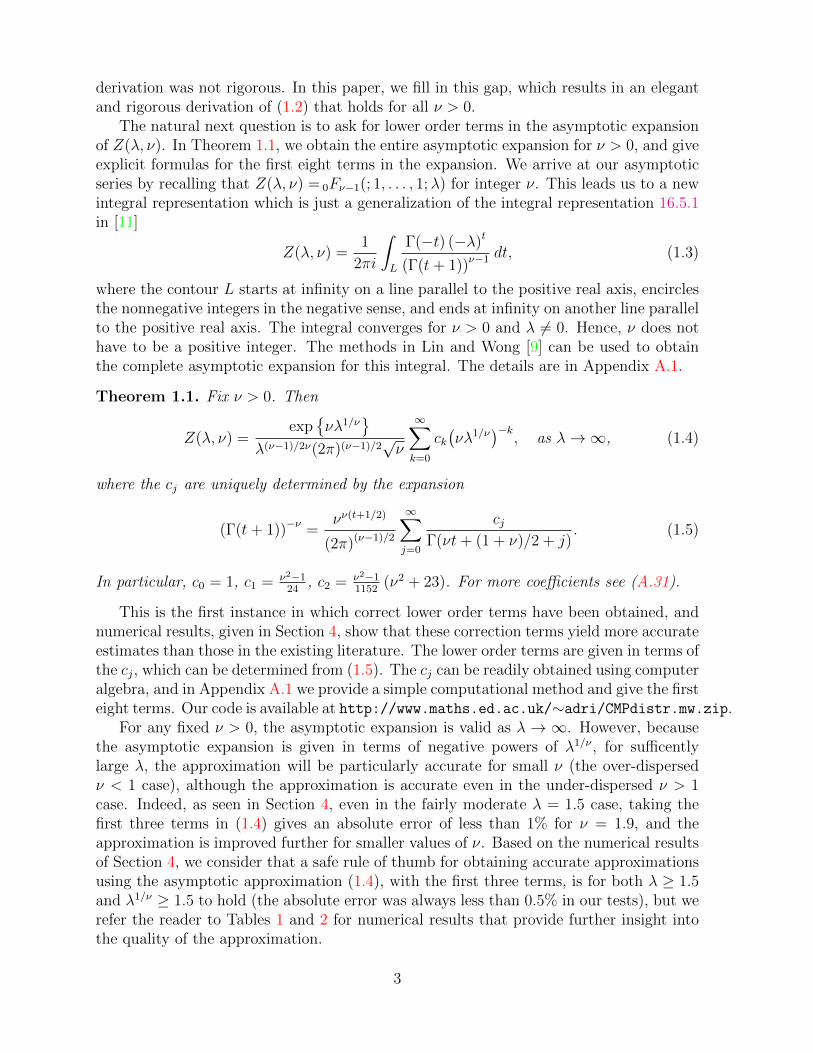
The natural next question is to ask for lower order terms in the asymptotic expansionof Z(λ, ν). In Theorem 1.1, we obtain the entire asymptotic expansion for ν > 0, and giveexplicit formulas for the first eight terms in the expansion. We arrive at our asymptoticseries by recalling that Z(λ, ν) = 0Fν−1(; 1, . . . , 1;λ) for integer ν. This leads us to a newintegral representation which is just a generalization of the integral representation 16.5.1in [11]

Z(λ, ν) =1

2πi

∫L

Γ(−t) (−λ)t

(Γ(t+ 1))ν−1dt, (1.3)

where the contour L starts at infinity on a line parallel to the positive real axis, encirclesthe nonnegative integers in the negative sense, and ends at infinity on another line parallelto the positive real axis. The integral converges for ν > 0 and λ 6= 0. Hence, ν does nothave to be a positive integer. The methods in Lin and Wong [9] can be used to obtainthe complete asymptotic expansion for this integral. The details are in Appendix A.1.

Theorem 1.1. Fix ν > 0. Then

Z(λ, ν) =exp

{νλ1/ν

}λ(ν−1)/2ν(2π)(ν−1)/2

√ν

∞∑k=0

ck(νλ1/ν

)−k, as λ→∞, (1.4)

where the cj are uniquely determined by the expansion

(Γ(t+ 1))−ν =νν(t+1/2)

(2π)(ν−1)/2

∞∑j=0

cjΓ(νt+ (1 + ν)/2 + j)

. (1.5)

In particular, c0 = 1, c1 = ν2−124

, c2 = ν2−11152

(ν2 + 23). For more coefficients see (A.31).

This is the first instance in which correct lower order terms have been obtained, andnumerical results, given in Section 4, show that these correction terms yield more accurateestimates than those in the existing literature. The lower order terms are given in terms ofthe cj, which can be determined from (1.5). The cj can be readily obtained using computeralgebra, and in Appendix A.1 we provide a simple computational method and give the firsteight terms. Our code is available at http://www.maths.ed.ac.uk/∼adri/CMPdistr.mw.zip.

For any fixed ν > 0, the asymptotic expansion is valid as λ → ∞. However, becausethe asymptotic expansion is given in terms of negative powers of λ1/ν , for sufficentlylarge λ, the approximation will be particularly accurate for small ν (the over-dispersedν < 1 case), although the approximation is accurate even in the under-dispersed ν > 1case. Indeed, as seen in Section 4, even in the fairly moderate λ = 1.5 case, taking thefirst three terms in (1.4) gives an absolute error of less than 1% for ν = 1.9, and theapproximation is improved further for smaller values of ν. Based on the numerical resultsof Section 4, we consider that a safe rule of thumb for obtaining accurate approximationsusing the asymptotic approximation (1.4), with the first three terms, is for both λ ≥ 1.5and λ1/ν ≥ 1.5 to hold (the absolute error was always less than 0.5% in our tests), but werefer the reader to Tables 1 and 2 for numerical results that provide further insight intothe quality of the approximation.

3

As mentioned above, certain important summary statistics of the CMP distributioncan be expressed in terms of the normalizing constant Z(λ, ν), and our asymptotic series(1.4) allows us to obtain more accurate estimates for these summaries than those in thecurrent literature. In Section 3, we demonstrate this by applying expansion (1.4) toobtain approximations for the mean, variance, cumulants, skweness, excess kurtosis andraw moments of CMP random variables.

The rest of this article is organised as follows. In Section 2, we fill in the gap inthe derivation of Simsek and Iyengar [19] to obtain a rigorous probabilistic proof of theleading term in the asymptotic expansion of Z(λ, ν). In Section 3, we use Theorem 1.1 toderive approximations for several summary statistics of the CMP distribution. In Section4, we present numerical results that confirm that the lower order correction terms resultin more accurate estimates of Z(λ, ν). We discuss our results in Section 5. Finally, inAppendix A, we prove Theorem 1.1 and the technical Lemma 2.1.

2 A probabilistic derivation of the leading term in

the expansion

In this section, we give a probabilistic derivation of the asymptotic formula (1.2). Thebasic approach is the same as the one given in Simsek and Iyengar [19], but additionalcare is taken to make the proof rigorous. After presenting our proof, we shall compare ourargument to theirs; see Remark 2.3. Before giving the proof we state a technical lemma,which we prove in Appendix A.2.

Lemma 2.1. Let Xα ∼ Po(α), where α > 0, and set Xα = Xα−α√α

. Let Z ∼ N(0, 1) havethe standard normal distribution. Suppose that h : R→ R does not depend on α.

(i) If h is differentiable with bounded derivative on R, then

E[h(Xα)] = E[h(Z)] +O(α−1/2), as α→∞.

(ii) If h is an even function (h(x) = h(−x) for all x ∈ R), and h is twice differentiablewith first and second derivative bounded on R, then

E[h(Xα)] = E[h(Z)] +O(α−1), as α→∞.

Proof of (1.2) for all ν > 0. For convenience let us reparametrize the CMP family withα = λ1/ν . Then the asymptotic formula (1.2) for C(α, ν) := Z(λ1/ν , ν) becomes

C(α, ν) =eνα

(2πα)ν−12√ν

[1 +O(α−1)

], as α→∞. (2.6)

The proof involves three steps. First, we write the normalising constant C(α, ν) as an ex-pectation of a function of the random variable Xα ∼ Po(α). We then obtain an asymptoticapproximation for this function, and finally use a normal approximation of the Poissonvariate Xα to approximate the expectations.

4

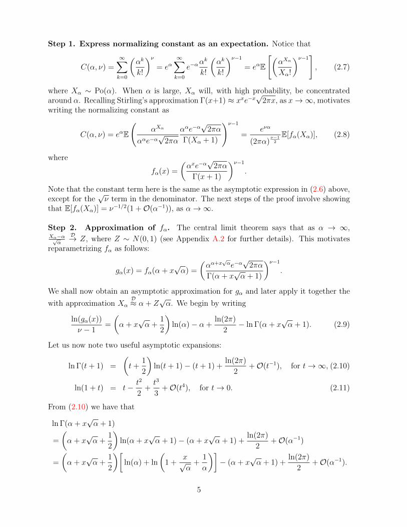
Step 1. Express normalizing constant as an expectation. Notice that

C(α, ν) =∞∑k=0

(αk

k!

)ν= eα

∞∑k=0

e−ααk

k!

(αk

k!

)ν−1= eαE

[(αXα

Xα!

)ν−1], (2.7)

where Xα ∼ Po(α). When α is large, Xα will, with high probability, be concentratedaround α. Recalling Stirling’s approximation Γ(x+1) ≈ xxe−x

√2πx, as x→∞, motivates

writing the normalizing constant as

C(α, ν) = eαE

(αXα

ααe−α√

2πα

ααe−α√

2πα

Γ(Xα + 1)

)ν−1

=eνα

(2πα)ν−12

E[fα(Xα)], (2.8)

where

fα(x) =

(αxe−α

√2πα

Γ(x+ 1)

)ν−1.

Note that the constant term here is the same as the asymptotic expression in (2.6) above,except for the

√ν term in the denominator. The next steps of the proof involve showing

that E[fα(Xα)] = ν−1/2(1 +O(α−1)), as α→∞.

Step 2. Approximation of fα. The central limit theorem says that as α → ∞,Xα−α√

α

D→ Z, where Z ∼ N(0, 1) (see Appendix A.2 for further details). This motivatesreparametrizing fα as follows:

gα(x) = fα(α + x√α) =

(αα+x

√αe−α√

2πα

Γ(α + x√α + 1)

)ν−1.

We shall now obtain an asymptotic approximation for gα and later apply it together the

with approximation XαD≈ α + Z

√α. We begin by writing

ln(gα(x))

ν − 1=

(α + x

√α +

1

2

)ln(α)− α +

ln(2π)

2− ln Γ(α + x

√α + 1). (2.9)

Let us now note two useful asymptotic expansions:

ln Γ(t+ 1) =

(t+

1

2

)ln(t+ 1)− (t+ 1) +

ln(2π)

2+O(t−1), for t→∞, (2.10)

ln(1 + t) = t− t2

2+t3

3+O(t4), for t→ 0. (2.11)

From (2.10) we have that

ln Γ(α + x√α + 1)

=

(α + x

√α +

1

2

)ln(α + x

√α + 1)− (α + x

√α + 1) +

ln(2π)

2+O(α−1)

=

(α + x

√α +

1

2

)[ln(α) + ln

(1 +

x√α

+1

α

)]− (α + x

√α + 1) +

ln(2π)

2+O(α−1).

5

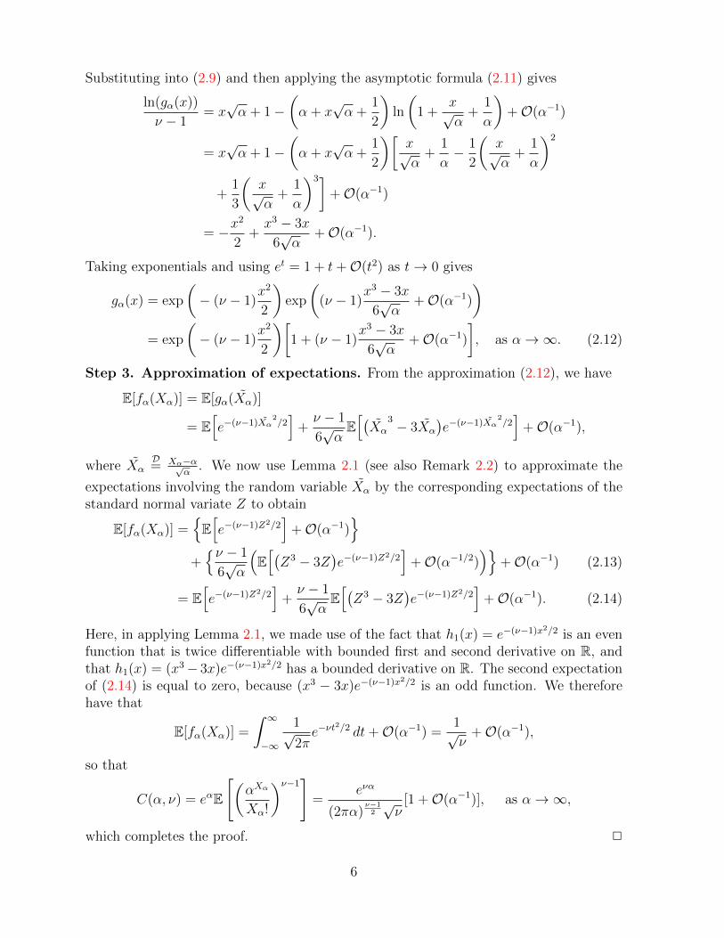
Substituting into (2.9) and then applying the asymptotic formula (2.11) gives

ln(gα(x))

ν − 1= x√α + 1−

(α + x

√α +

1

2

)ln

(1 +

x√α

+1

α

)+O(α−1)

= x√α + 1−

(α + x

√α +

1

2

)[x√α

+1

α− 1

2

(x√α

+1

α

)2

+1

3

(x√α

+1

α

)3]+O(α−1)

= −x2

2+x3 − 3x

6√α

+O(α−1).

Taking exponentials and using et = 1 + t+O(t2) as t→ 0 gives

gα(x) = exp

(− (ν − 1)

x2

2

)exp

((ν − 1)

x3 − 3x

6√α

+O(α−1)

)= exp

(− (ν − 1)

x2

2

)[1 + (ν − 1)

x3 − 3x

6√α

+O(α−1)

], as α→∞. (2.12)

Step 3. Approximation of expectations. From the approximation (2.12), we have

E[fα(Xα)] = E[gα(Xα)]

= E[e−(ν−1)Xα

2/2]

+ν − 1

6√αE[(Xα

3 − 3Xα

)e−(ν−1)Xα

2/2]

+O(α−1),

where XαD= Xα−α√

α. We now use Lemma 2.1 (see also Remark 2.2) to approximate the

expectations involving the random variable Xα by the corresponding expectations of thestandard normal variate Z to obtain

E[fα(Xα)] ={E[e−(ν−1)Z

2/2]

+O(α−1)}

+{ν − 1

6√α

(E[(Z3 − 3Z

)e−(ν−1)Z

2/2]

+O(α−1/2))}

+O(α−1) (2.13)

= E[e−(ν−1)Z

2/2]

+ν − 1

6√αE[(Z3 − 3Z

)e−(ν−1)Z

2/2]

+O(α−1). (2.14)

Here, in applying Lemma 2.1, we made use of the fact that h1(x) = e−(ν−1)x2/2 is an even

function that is twice differentiable with bounded first and second derivative on R, andthat h1(x) = (x3− 3x)e−(ν−1)x

2/2 has a bounded derivative on R. The second expectationof (2.14) is equal to zero, because (x3 − 3x)e−(ν−1)x

2/2 is an odd function. We thereforehave that

E[fα(Xα)] =

∫ ∞−∞

1√2πe−νt

2/2 dt+O(α−1) =1√ν

+O(α−1),

so that

C(α, ν) = eαE

[(αXα

Xα!

)ν−1]=

eνα

(2πα)ν−12√ν

[1 +O(α−1)], as α→∞,

which completes the proof. 2

6

Remark 2.2. Using Lemma 2.1 allows us to quantify the size of the error in the approx-imation (2.13). We could have derived the leading term in the asymptotic formula (1.2)through a simpler argument by appealing to the fact that since Xα convergences in distri-bution to the standard normal distribution we have that E[h(Xα)]→ E[h(Z)], as α→∞,for all bounded functions h : R → R. However, this would have led to the weaker resultthat C(α, ν) = eνα

(2πα)ν−12√ν

[1 + o(1)], as α→∞.

Remark 2.3. The basic outline of our proof follows that of Simsek and Iyengar [19],

who used the approximation 2√Xα

D≈ N(2

√α, 1), or Xα

D≈ α + Z

√α + Z2

4. Instead, here

we use the central limit approximation XαD≈ α + Z

√α, which is simpler and leads to

no error terms of larger order. Most importantly, our approach allows us to appeal toresults for approximating expectations from the Stein’s method literature. Applying theseresults allows us to make the derivation rigorous and quantify the size of the error in theapproximation.

3 Applications: approximation of summary statistics

Many important summary statistics, such as moments and cumulants, of the CMP dis-tribution can be expressed in terms of the normalizing constant Z(λ, ν); see Section 2 ofDaly and Gaunt [3] for a comprehensive account, where all formulas below can be found.

Let X ∼ CMP(λ, ν). The probability generating function is EsX = Z(sλ,ν)Z(λ,ν)

, and the meanand variance are given by

EX = λd

dλ

{ln(Z(λ, ν))

}, (3.15)

Var(X) = λd

dλEX. (3.16)

The cumulant generating function is

g(t) = ln(E[etX ]) = ln(Z(λet, ν))− ln(Z(λ, ν)),

and the cumulants are given by

κn = g(n)(0) =∂n

∂tnln(Z(λet, ν))

∣∣∣∣t=0

, n ≥ 1. (3.17)

The skewness γ1 = κ3σ3 and excess kurtosis γ2 = κ4

σ4 , where σ2 = Var(X), can therefore alsobe expressed in terms of Z(λ, ν). As moments can be expressed in terms of cumulants, itfollows that they in turn can be expressed in terms of Z(λ, ν). Let µ′n = EXn. Then

µ′n =n∑k=1

Bn,k(κ1, . . . , κn−k+1), (3.18)

where the partial Bell polynomial (see Hazelwinkel [6], p. 96) is given by

Bn,k(x1, x2, . . . , xn−k+1) =∑ n!

j1!j2! · · · jn−k+1!

(x11!

)j1(x22!

)j2· · ·(

xn−k+1

(n− k + 1)!

)jn−k+1

,

7

where the sum is taken over all sequences j1, j2, j3, . . . , jn−k+1 of non-negative integerssuch that the following two conditions hold:

j1 + j2 + · · ·+ jn−k+1 = k,

j1 + 2j2 + 3j3 + · · ·+ (n− k + 1)jn−k+1 = n.

The central moments µn = E[(X − EX)n] can be obtained by setting κ1 = 0 in (3.18).For general parameter values, there do not exist simple closed form formulas for these

summary statistics. However, due to the asymptotic approximations of Z(λ, ν), we canobtain approximations. Shmueli et al. [18] used the formula (3.15) and the approximation(1.2) for the normalizing constant to obtain the approximation

EX ≈ λ1/ν − ν − 1

2ν, as λ→∞. (3.19)

Their result was given for integer ν, but as the approximation (1.2) has since been shownto be valid for all ν > 0, it follows that (3.19) also holds for all ν > 0. Daly and Gaunt [3]used the approximation (1.2) to derive the leading order term in the asymptotic expansionof a number of further summary statistics, which hold for all ν > 0.

In the following proposition, we use the asymptotic expansion (1.4) to obtain ad-ditional correction terms for several important summary statistics. The expansions wepresent include the first four terms in the asymptotic series for the above summary statis-tics, except for the moments for which we obtain the first three terms owing to morecomplicated expressions. With further calculations, one could readily obtain additionalterms, although this would complicate the exposition and lead to only negligible improve-ments in accuracy.

Proposition 3.1. Let X ∼ CMP(λ, ν), where ν > 0. Then, as λ→∞,

EX = λ1/ν(

1− ν − 1

2νλ−1/ν − ν2 − 1

24ν2λ−2/ν − ν2 − 1

24ν3λ−3/ν +O(λ−4/ν)

), (3.20)

Var(X) =λ1/ν

ν

(1 +

ν2 − 1

24ν2λ−2/ν +

ν2 − 1

12ν3λ−3/ν +O(λ−4/ν)

), (3.21)

κn =λ1/ν

νn−1

(1 +

(−1)n(ν2 − 1)

24ν2λ−2/ν +

(−2)n(ν2 − 1)

48ν3λ−3/ν +O(λ−4/ν)

), (3.22)

γ1 =λ−1/2ν√

ν

(1− 5(ν2 − 1)

48ν2λ−2/ν − 7(ν2 − 1)

24ν3λ−3/ν +O(λ−4/ν)

), (3.23)

γ2 =λ−1/ν

ν

(1− (ν2 − 1)

24ν2λ−2/ν +

(ν2 − 1)

6ν3λ−3/ν +O(λ−4/ν)

), (3.24)

µ′n = λn/ν(

1 +n(n− ν)

2νλ−1/ν + a2λ

−2/ν +O(λ−3/ν)

), (3.25)

where

a2 = −n(ν − 1)(6nν2 − 3nν − 15n+ 4ν + 10)

24ν2+

1

ν2

{(n

3

)+ 3

(n

4

)}.

The asymptotic series (3.22) for κn holds for all n ≥ 2, and κ1 = EX.

8

Proof. We start with the mean. To obtain the desired level of accuracy it suffices totruncate the asymptotic series (1.4) for Z(λ, ν) at the third term:

Z(λ, ν) =exp

{νλ1/ν

}λ(ν−1)/2ν(2π)(ν−1)/2

√ν

(1 + c1

(νλ1/ν

)−1+ c2

(νλ1/ν

)−2+O(λ−3/ν)

),

as λ→∞. Taking logarithms gives

ln(Z(λ, ν)) = νλ1/ν − ν − 1

2νln(λ) + Cν + ln

(1 + c1ν

−1λ−1/ν + c2ν−2λ−2/ν +O(λ−3/ν)

).

where Cν = − ln((2π)(ν−1)/2

√ν). Applying the asymptotic formula

ln(1 + ax+ bx2 +O(x3)) = ax+ (b− a2/2)x2 +O(x3), as x→ 0,

then yields

ln(Z(λ, ν)) = νλ1/ν − ν − 1

2νln(λ) +Cν +

c1νλ−1/ν +

(c2 − c21/2)

ν2λ−2/ν +O(λ−3/ν). (3.26)

We now differentiate the asymptotic series to obtain

EX = λd

dλ

{ln(Z(λ, ν))

}= λ1/ν − ν − 1

2ν− c1ν2λ−1/ν − 2

ν3(c2 − c21/2)λ−2/ν +O(λ−3/ν),

which on recalling that c1 = ν2−124

and noting that c2 − c21/2 = ν2−148

yields the desiredasymptotic series for the mean. Here we differentiated the asymptotic series (3.26) in thenaive sense by simply differentiating term by term. This is justifiable here (and throughoutthis proof) because the remainder term is of the form

∑∞k=3 akλ

−k/ν . However, as notedby [7], p. 23, asymptotic series cannot be differentiated in this manner in general. Theasymptotic series (3.21) for the variance now follows from differentiating the series (3.20)and applying the formula (3.16).

We now move on to the cumulants. As κ1 = EX, we restrict our attention to n ≥ 2.From (3.26) we have

ln(Z(λet, ν)) = νλ1/νet/ν − ν − 1

2νt+ Cλ,ν + c1

(νλ1/νet/ν

)−1+ (c2 − c21/2)

(νλ1/νet/ν

)−2+O(λ−3/ν),

where Cλ,ν = −ν−12ν

ln(λ) + Cν . Using (3.17) and differentiating gives, for n ≥ 2,

κn =∂n

∂tnln(Z(λet, ν))

∣∣∣∣t=0

=λ1/ν

νn−1+

(−1)nc1νn+1

λ−1/ν +(−2)n(c2 − c21/2)

νn+2λ−2/ν +O(λ−3/ν),

which on substituting c1 = ν2−124

and c2 − c21/2 = ν2−148

yields (3.22).We now obtain the asymptotic expansions for the skewness γ1 = κ3

σ3 and excess kurtosisγ2 = κ4

σ4 . From (3.22), (3.23) and (3.21) we have

γ1 =λ−1/2ν√

ν

(1− ν2 − 1

24ν2λ−2/ν − ν2 − 1

6ν3λ−3/ν +O(λ−4/ν)

)×(

1 +ν2 − 1

24ν2λ−2/ν +

ν2 − 1

12ν3λ−3/ν +O(λ−4/ν)

)−3/2, (3.27)

9

and

γ2 =λ−1/ν

ν

(1 +

ν2 − 1

24ν2λ−2/ν +

ν2 − 1

3ν3λ−3/ν +O(λ−4/ν)

)×(

1 +ν2 − 1

24ν2λ−2/ν +

ν2 − 1

12ν3λ−3/ν +O(λ−4/ν)

)−2. (3.28)

Applying the asymptotic formula

1 + ax2 + bx3

(1 + cx2 + dx3)n= 1 + (a− nc)x2 + (b− nd)x3 +O(x4), as x→ 0,

with n = 3/2 and n = 2 to (3.27) and (3.28), respectively, then yields (3.23) and (3.24).Finally, we obtain the asymptotic expansions for the moments µ′n. Note that κ1, . . . , κn

are all of order λ1/ν as λ→∞. Hence, from (3.18) and the asymptotic expansions (3.20)for EX = κ1 and (3.22) for the cumulants κn, we have

µ′n = κn1 +

(n

2

)κn−21 κ2 +

(n

3

)κn−31 κ3 + 3

(n

4

)κn−41 κ22 +O(λ(n−3)/ν)

= λn/ν(

1− ν − 1

2νλ−1/ν − ν2 − 1

24ν2λ−2/ν +O(λ−3/ν)

)n+λ(n−1)/ν

ν

(n

2

)(1− ν − 1

2νλ−1/ν +O(λ−2/ν)

)n−2(1 +O(λ−2/ν)

)+λ(n−2)/ν

ν2

{(n

3

)+ 3

(n

4

)}+O(λ(n−3)/ν)

= λn/ν +

{− n(ν − 1)

2ν+

1

ν

(n

2

)}λ(n−1)/ν +

{(n

2

)(ν − 1

2ν

)2

− n(ν2 − 1)

24ν2

− 1

ν

(n

2

)(n− 2)(ν − 1)

2ν+

1

ν2

{(n

3

)+ 3

(n

4

)}}λ(n−2)/ν +O(λ(n−3)/ν),

which on simplifying yields (3.25). The proof is complete.

4 Numerical results

Tables 1 and 2 give the percentage errors in approximating the normalizing Z(λ, ν) bythe asymptotic series (1.4). The values of λ and ν in Table 1 are the same as those usedby Shumeli et al. [18], who also looked at the percentage errors of the leading term in theapproximation. The values of λ and ν given in Table 2 provide additional insight into thequality of the approximation in a different parameter regime. Looking at Table 1, we seethat when λ is small the approximation underestimates Z(λ, ν), and the approximationis particularly poor when ν is also small. In these cases, including additional correctionsterms actually leads to a worse approximation. However, as expected, the approximationimproves as λ increases, particularly when λ1/ν increases. For λ ≥ 1.1, including thefirst correction term always leads to a more accurate approximation, and when λ ≥ 1.5

10

Table 1: Percentage error for the approximation of Z(λ, ν) by the leading order term, with first ordercorrection, and with second order correction in (1.4). A negative number means that the approximationis less than the true value. Errors greater than 100% are denoted by 101.

HHHHλ

ν0.1 0.3 0.5 0.7 0.9 1.1 1.3 1.5 1.7 1.9

0.1 −100 −78.7 −35.8 −10.8 −1.39 0.106 −1.89 −5.24 −8.96 −12.60.1 −101 −101 −101 −83.4 −12.6 6.57 10.9 10.0 7.38 4.190.1 −101 −101 −101 −101 −92.3 30.6 40.5 34.9 27.5 20.7

0.3 −97.7 −38.4 −6.81 1.10 1.08 −1.37 −4.42 −7.44 −10.2 −12.70.3 −101 −101 −71.5 −16.0 −2.31 0.974 0.918 −0.268 −1.78 −3.310.3 −101 −101 −101 −83.0 −9.42 4.19 6.25 5.34 3.66 1.87

0.5 −83.3 −12.0 2.87 3.70 1.42 −1.45 −4.24 −6.77 −9.02 −11.00.5 −101 −101 −22.9 −4.77 −0.505 0.023 −0.631 −1.64 −2.68 −3.660.5 −101 −101 −101 −20.7 −2.80 1.29 1.80 1.23 0.338 −0.5750.7 −49.1 2.16 6.05 4.16 1.38 −1.33 −3.78 −5.96 −7.86 −9.540.7 −101 −40.2 −7.47 −1.11 0.058 −0.244 −0.985 −1.81 −2.56 −3.290.7 −101 −101 −34.2 −7.23 −1.03 0.444 0.473 0.030 −0.538 −1.090.9 −8.59 7.77 6.59 3.93 1.25 −1.18 −3.34 −5.24 −6.91 −8.390.9 −101 −11.6 −1.63 0.258 0.248 −0.315 −1.02 −1.71 −2.32 −2.850.9 −101 −55.7 −11.5 −2.72 −0.372 0.121 −0.022 −0.377 −0.775 −1.141.1 9.76 8.51 6.05 3.48 1.10 −1.04 −2.94 −4.64 −6.15 −7.491.1 −7.70 −1.47 0.575 0.740 0.300 −0.317 −0.949 −1.53 −2.04 −2.461.1 −40.0 −13.1 −3.81 −0.933 −0.097 −0.014 −0.215 −0.507 −0.802 −1.061.3 4.80 7.08 5.15 3.00 0.960 −0.915 −2.61 −4.14 −5.53 −6.771.3 1.67 1.43 1.26 0.853 0.296 −0.294 −0.852 −1.35 −1.78 −2.131.3 0.576 −2.34 −0.970 −0.180 0.023 −0.069 −0.283 −0.527 −0.755 −0.9441.5 0.813 5.09 4.20 2.56 0.835 −0.809 −2.34 −3.74 −5.02 −6.191.5 0.092 1.65 1.31 0.812 0.270 −0.263 −0.754 −1.19 −1.55 −1.851.5 0.032 0.227 0.062 0.129 0.072 −0.090 −0.296 −0.503 −0.686 −0.8291.7 0.210 3.36 3.36 2.17 0.729 −0.719 −2.10 −3.40 −4.60 −5.711.7 0.005 1.14 1.12 0.713 0.238 −0.231 −0.662 −1.04 −1.36 −1.631.7 0.000 0.526 0.371 0.237 0.087 −0.093 −0.284 −0.462 −0.612 −0.7241.9 0.068 2.14 2.65 1.84 0.639 −0.643 −1.91 −3.11 −4.25 −5.301.9 0.001 0.620 0.875 0.600 0.205 −0.202 −0.581 −0.918 −1.20 −1.441.9 0.000 0.333 0.398 0.255 0.088 −0.089 −0.262 −0.416 −0.543 −0.633

including both the first and second order correction always leads to the most accurateestimate. For λ = 1.9, including second order correction gives estimates that are moreaccurate by an order of magnitude than using just the leading order term, and the absoluteerror is always less than 1%. One can also see from Table 1 that the approximation isparticularly accurate when ν is close to 1. This is to be expected because when ν = 1the leading term in the asymptotic expansion (1.4) reduces, for all λ > 0, to eλ, meaningthat the approximation is exact since Z(λ, 1) = eλ.

We carried out a similar analysis for the mean, variance, skewness and excess kurtosis.We obtained very similar results, which is unsurprising given that all the these summarystatistics can be expressed in terms of Z(λ, ν). For space reasons, we omit the results.

Lastly, we remark that the largest value of the normalizing constant in our studywas Z(1.9, 0.1) = 5.49743309747796 × 1028. For larger λ, approximating Z(λ, ν) bytruncating the exact sum at some large value would be computationally challenging,whereas the asymptotic approximation (1.4) offers an accurate and computationally ef-ficient alternative. Indeed, taking eight terms in the asymptotic approximation gives us5.49743309747884× 1028, and hence the relative error is 1.59× 10−13.

11

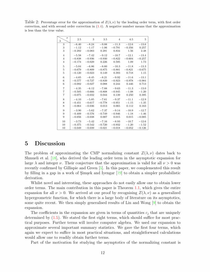
Table 2: Percentage error for the approximation of Z(λ, ν) by the leading order term, with first ordercorrection, and with second order correction in (1.4). A negative number means that the approximationis less than the true value.

HHHHλ

ν2.5 3 3.5 4 4.5 5

3 −6.40 −8.24 −9.88 −11.3 −12.6 −13.63 −1.12 −1.17 −1.06 −0.791 −0.356 0.2573 −0.292 −0.083 0.291 0.834 1.56 2.48

4 −5.58 −7.42 −9.12 −10.7 −12.1 −13.44 −0.838 −0.936 −0.930 −0.822 −0.604 −0.2574 −0.174 −0.029 0.226 0.595 1.09 1.73

5 −5.04 −6.86 −8.60 −10.3 −11.8 −13.35 −0.679 −0.809 −0.875 −0.881 −0.821 −0.6755 −0.120 −0.023 0.149 0.393 0.718 1.15

6 −4.65 −6.45 −8.21 −9.92 −11.6 −13.16 −0.577 −0.727 −0.839 −0.923 −0.978 −0.9846 −0.092 −0.027 0.088 0.244 0.446 0.713

7 −4.35 −6.12 −7.88 −9.63 −11.3 −13.07 −0.505 −0.666 −0.808 −0.945 −1.08 −1.207 −0.075 −0.032 0.044 0.139 0.250 0.395

8 −4.10 −5.85 −7.61 −9.37 −11.1 −12.98 −0.451 −0.617 −0.778 −0.951 −1.15 −1.358 −0.064 −0.036 0.013 0.065 0.112 0.163

9 −3.90 −5.62 −7.37 −9.14 −10.9 −12.79 −0.409 −0.576 −0.749 −0.946 −1.18 −1.469 −0.056 −0.038 0.007 0.015 0.015 −0.00510 −3.73 −5.42 −7.16 −8.93 −10.7 −12.610 −0.375 −0.542 −0.720 −0.932 −1.20 −1.5210 −0.049 −0.039 −0.021 −0.018 −0.052 −0.126

5 Discussion

The problem of approximating the CMP normalizing constant Z(λ, ν) dates back toShmueli et al. [18], who derived the leading order term in the asymptotic expansion forlarge λ and integer ν. Their conjecture that the approximation is valid for all ν > 0 wasrecently confirmed by Gillispie and Green [5]. In this paper, we complemented this resultby filling in a gap in a work of Simsek and Iyengar [19] to obtain a simpler probabilisticderivation.

Whilst novel and interesting, these approaches do not easily allow one to obtain lowerorder terms. The main contribution in this paper is Theorem 1.1, which gives the entireexpansion for all ν > 0. We arrived at our proof by recognising Z(λ, ν) as a generalizedhypergeometric function, for which there is a large body of literature on its asymptotics,some quite recent. We then simply generalised results of Lin and Wong [9] to obtain theexpansion.

The coefficients in the expansion are given in terms of quantities cj that are uniquelydetermined by (1.5). We stated the first eight terms, which should suffice for most prac-tical purposes. Further terms will involve computer algebra. We used our expansion toapproximate several important summary statistics. We gave the first four terms, whichagain we expect to suffice in most practical situations, and straightforward calculationswould allow one to readily obtain further terms.

Part of the motivation for studying the asymptotics of the normalizing constant is

12

that many important summary statistics can be expressed in terms of it. However, thereare of course important summaries that do not involve such simple representations, suchas the median. We were therefore unable to exploit our asymptotic series to improveon the current best approximation of Daly and Gaunt [3]. We leave this and relatedapproximations as interesting further open problems.

A Further proofs

A.1 Proof of Theorem 1.1

The generalized hypergeometric function is defined by

pFq

(a1, . . . , apb1, . . . , bq

; z

)=∞∑k=0

(a1)n · · · (ap)n(b1)n · · · (bq)n

zn

n!,

provided none of the bj are nonpositive integers, where the Pochhammer symbol is (a)0 = 1and (a)n = a(a + 1)(a + 2) · · · (a + n − 1), n ≥ 1. In the case that p ≤ q the infiniteseries converges for all finite values of z and defines an entire function. For more detailssee §16.2 in [11]. As noted by Nadarajah [10], Z(λ, ν) = 0Fν−1(; 1, . . . , 1;λ) for integerν. Thus, we can exploit the well-developed theory for asymptotics of the generalizedhypergeometric function to obtained an asymptotic expansion for Z(λ, ν) when ν is aninteger. Indeed, 16.11.9 in [11] can be used to write down the entire expansion for integerν. However, this expansion is only valid for integer ν, and, since b1 = · · · = bν−1 = 1,the coefficients of the lower order terms in the expansion must be obtained via a tediouslimiting procedure. We can, however, make use of a recent work on the asymptotics ofthe generalized hypergeometric function to prove Theorem 1.1.

Proof of Theorem 1.1. We obtain the expansion (1.4) by appealing to results fromthe recent work of Lin and Wong [9], in which the large z asymptotics of the generalized

hypergeometric function pFq

(a1,··· ,apb1,··· ,bq ; z

)are discussed. Here we will have p = 0, all the

bk = 1 and q = ν − 1. In the proof of Lemma 4.3 in [9] it is not essential that q is anonnegative integer and below we copy the main steps.

Lin and Wong [9] used as their starting point the integral representation 16.5.1 in[11] of the generalized hypergeometric function. As mentioned in the introduction, theintegral representation (1.3) is just a simple generalization of 16.5.1 in [11]. We rewriteit as

Z(λ, ν) =1

2πi

∫L

Γ(t+ 1)Γ(−t) (−λ)t

(Γ(t+ 1))νdt, (A.29)

and use the inverse factorial expansion (again, see [9], or §2.2.2 in Paris and Kaminski[13], and for more information about factorial series see Weniger [21])

(Γ(t+ 1))−ν =νν(t+1/2)

(2π)(ν−1)/2

∞∑j=0

cjΓ(νt+ (1 + ν)/2 + j)

, (A.30)

13

in the integral in (A.29) and combine this with the proof of Lemma 4.3 in [9]. The resultis asymptotic expansion (1.4).

To compute the cj we substitute the Stirling approximation

Γ(x) ∼ e−xxx(

2π

x

)1/2 ∞∑k=0

gkxk, x→∞,

(see 5.11.3 in [11]) into both sides of (A.30). Here g0 = 1, g1 = 112

, g2 = 1288

, and furthervalues are given in 5.11.4 – 5.11.6 in [11]. In this way we obtain large t asymptoticexpansions for both sides of (A.30) and we can compare the coefficients to find the cj.Computer algebra is very useful for this process; we used Maple to obtain the first eightcoefficients. The result is:

c0 = 1, c1 =ν2 − 1

24, c2 =

ν2 − 1

1152

(ν2 + 23

), c3 =

ν2 − 1

414720

(5ν4 − 298ν2 + 11237

),

c4 =ν2 − 1

39813120

(5ν6 − 1887ν4 − 241041ν2 + 2482411

),

c5 =ν2 − 1

6688604160

(7ν8 − 7420ν6 + 1451274ν4 − 220083004ν2 + 1363929895

),

c6 =ν2 − 1

4815794995200

(35ν10 − 78295ν8 + 76299326ν6 + 25171388146ν4 (A.31)

−915974552561ν2 + 4175309343349),

c7 =ν2 − 1

115579079884800

(5ν12 − 20190ν10 + 45700491ν8 − 19956117988ν6

+7134232164555ν4 − 142838662997982ν2 + 525035501918789).

2

A.2 Proof of Lemma 2.1

Let us first note two results that were derived using Stein’s method. Theorem A.1 isproved in Stein [20], whilst Theorem A.2 is a special (and slightly simplified) case of thegeneral bound of Theorem 3.5 of Gaunt [4]. The simplified bound is, however, sufficientlytight for the purpose of proving part (ii) of Lemma 2.1.

Theorem A.1. Stein [20], (1986). Let X1, . . . , Xn be i.i.d. random variables with EX1 =0, EX2

1 = 1 and E|X1|3 < ∞. Set W = 1√n

∑ni=1Xi and let Z ∼ N(0, 1). Suppose

h : R→ R has a bounded first derivative on R. Then

|E[h(W )]− E[h(Z)]| ≤ ‖h′‖∞√n

(2 + E|X1|3

),

where ‖h′‖∞ = supx∈R |h′(x)|.

Theorem A.2. Gaunt [4], (2015). Let X1, . . . , Xn and W be defined as in Theorem A.1,but with the additional assumption that E|X1|6 < ∞. Suppose h : R → R is an even

14

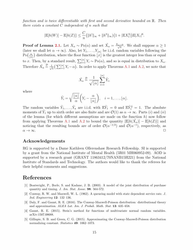
function and is twice differentiable with first and second derivative bounded on R. Thenthere exists a constant C independent of n such that

|E[h(W )]− E[h(Z)]| ≤ C

n

(‖h′‖∞ + ‖h′′‖∞)

(1 + |EX3

1 |)E|X1|6.

Proof of Lemma 2.1. Let Xα ∼ Po(α) and set Xα = Xα−α√α

. We shall suppose α ≥ 1

(later we shall let α→∞). Also, let Y1, . . . , Ybαc be i.i.d. random variables following thePo(αbαc

)distribution, where the floor function bxc is the greatest integer less than or equal

to x. Then, by a standard result,∑bαc

i=1 Yi ∼ Po(α), and so is equal in distribution to Xα.

Therefore XαD= 1√

α

(∑bαci=1 Yi−α

). In order to apply Theorems A.1 and A.2, we note that

XαD=

1√bαc

bαc∑i=1

Yi,

where

Yi =

√bαcα

(Yi −

α

bαc

), i = 1, . . . , bαc.

The random variables Y1, . . . , Yn are i.i.d. with EY1 = 0 and EY 21 = 1. The absolute

moments of Y1 up to sixth order are also finite and are O(1) as α→∞. Parts (i) and (ii)of the lemma (for which different assumptions are made on the function h) now followfrom applying Theorems A.1 and A.2 to bound the quantity |E[h(Xα)] − E[h(Z)]| andnoticing that the resulting bounds are of order O(α−1/2) and O(α−1), respectively, asα→∞. 2

Acknowledgements

RG is supported by a Dame Kathleen Ollerenshaw Research Fellowship. SI is supportedby a grant from the National Institute of Mental Health (5R01 MH060952-09). AOD issupported by a research grant (GRANT 11863412/70NANB15H221) from the NationalInstitute of Standards and Technology. The authors would like to thank the referees fortheir helpful comments and suggestions.

References

[1] Boatwright, P., Borle, S. and Kadane, J. B. (2003). A model of the joint distribution of purchasequantity and timing. J. Am. Stat. Assoc. 98: 564-572.

[2] Conway, R. W. and Maxwell, W. L. (1962). A queueing model with state dependent service rate. J.Ind. Engineering 12: 132–136.

[3] Daly, F. and Gaunt, R. E. (2016). The Conway-Maxwell-Poisson distribution: distributional theoryand approximation. ALEA Lat. Am. J. Probab. Math. Stat. 13: 635–658.

[4] Gaunt, R. E. (2015). Stein’s method for functions of multivariate normal random variables.arXiv:1507.08688.

[5] Gillispie, S. B. and Green, C. G. (2015). Approximating the Conway-Maxwell-Poisson distributionnormalizing constant. Statistics 49: 1062–1073.

15

[6] Hazelwinkel, M. (1997). Encyclopedia of Mathematics, Supplement I., Kluwer Academic Publishers,Dordrehct.

[7] Hinch, E. J. (1991). Perturbation Methods. Cambridge University Press, Cambridge.

[8] Kadane, J. B., Shmueli, G., Minka, T. P., Borle, S. and Boatwright, P. (2006). Conjugate analysisof the Conway-Maxwell-Poisson distribution. Bayesian Anal. 1: 403–420.

[9] Lin, Y. and Wong, R. (2017). Asymptotics of Generalized Hypergeometric Functions. Frontiers ofOrthogonal Polynomials and q-Series, World Scientific, Singapore, preprint.

[10] Nadarajah, S. (2009). Useful moment and CDF formulations for the COM-Poisson distribution. Stat.Papers 50: 617–622.

[11] NIST Digital Library of Mathematical Functions. http://dlmf.nist.gov/, Release 1.0.12 of 2016-09-09. F. W. J. Olver, A. B. Olde Daalhuis, D. W. Lozier, B. I. Schneider, R. F. Boisvert, C. W. Clark,B. R. Miller and B. V. Saunders, eds.

[12] Olver, F. W J. (1974). Asymptotics and Special Functions. New York: Academic Press.

[13] Paris, R. B. and Kaminski, D. (2001). Asymptotics and Mellin-Barnes Integrals. Cambridge Univer-sity Press.

[14] Pogany, T. K. (2016). Integral form of the COM-Poisson renormalization constant. Stat. Probabil.Lett. 116: 144–145.

[15] Rodrigues, J., de Castro, M., Cancho, V. G. and Balakrishnan, N. (2009). COM-Poisson cure ratesurvival models and an application to a cutaneous melanoma data. J. Statist. Plann. Inference 139:3605–3611.

[16] Sellers, K. F., Borle, S. and Shmueli, G. (2012). The COM-Poisson model for count data: A surveyof methods and applications. Appl. Stoch. Model. Bus. 28: 104–116.

[17] Sellers, K. F. and Shmueli, G. (2010). A flexible regression model for count data. Ann. Appl. Stat.4: 943–961.

[18] Shmueli, G., Minka, T. P., Kadane, J. B., Borle, S. and Boatwright, P. (2005). A useful distributionfor fitting discrete data: Revival of the COM-Poisson. J. R. Stat Soc. Ser. C 54: 127–142.

[19] Simsek B. and Iyengar S. (2016). Approximating the Conway-Maxwell-Poisson normalizing constant.Filomat 30: 953–960.

[20] Stein, C. (1986). Approximate Computation of Expectations. IMS, Hayward, California.

[21] Weniger, E. J. (2010). Summation of divergent power series by means of factorial series. Appl. Numer.Math., 60: 1429–1441.

16