An Assessment of the Impact of Wheat Market Liberalization in Egypt: A Multi-

Market Model Approach

Gamal M. Siam and André Croppenstedt

ESA Working Paper No. 07-15

May 2007

www.fao.org/es/esa

Agricultural Development Economics Division

The Food and Agriculture Organization of the United Nations

2

ESA Working Paper No. 07-15 www.fao.org/es/esa

An Assessment of the Impact of Wheat Market Liberalization in Egypt: A Multi-Market Model Approach1

May 2007

Gamal M. Siam

Department of Agricultural Economics Faculty of Agriculture, Cairo University, Giza,

Egypt e:mail: gamal_siam@hotmail.com

André Croppenstedt Agricultural Development

Economics Division Food and Agriculture Organization

Italy e-mail: andre.croppenstedt@fao.org

Abstract Wheat is central to the government of Egypt’s food security policy which is influenced by a concern for overdependence on imports and the need to provide subsidized bread for the poor. This paper uses a multi-market approach to assess the impact of complete wheat market liberalization, an international wheat price increase, the value of strategic stocks and the impact of investment to generate higher yields and lower transaction costs for wheat producers. Results show that wheat market liberalization implies very substantial costs for consumers and producers. The estimated income losses that these groups suffer would appear to be below the current total subsidy costs and hence a cash transfer program would, in principle, be feasible. The results show that wheat price movements impact strongly on the supply and/or demand side in particular of berseem, rice, maize, cotton and livestock which has significant implications for their net imports as well as input use. Results indicate that strategic stocks can be useful to neutralize the impact of a wheat price spike. Increasing wheat yields and reducing transportation boosts wheat self-sufficiency but does not dampen the impact of removing the wheat subsidy system on household’s welfare.

Key Words: Egypt, agriculture sector, wheat, multi-market model, bread subsidy, policy scenario impact analysis.

JEL: Q11, Q18. The designations employed and the presentation of material in this information product do not imply the expression of any opinion whatsoever of the part of the Food and Agriculture Organization of the United Nations concerning the legal status of any country, territory, city or area or of its authorities, or concerning the delimitation of its frontiers or boundaries.

1 This paper was prepared as part of the “Linking Agriculture Policies to Poverty and Food Security” module of

the Roles of Agriculture Project. The designations employed and the presentation of material in this information product do not imply the expression of any opinion whatsoever on the part of the Food and Agriculture Organization of the United Nations concerning the legal status of any country, territory, city or area or of its authorities, or concerning the delimitation of its frontiers or boundaries. Content and errors are exclusively the responsibility of the author and do not necessarily reflect the position of the Food and Agriculture Organization of the UN or of Cairo University. Content and errors are exclusively the responsibility of the authors and not the FAO or the authors’ institution. The multi-market model developed for this study builds on Lundberg and Rich (2002) and Stifel and Randrianarisoa (2004). We are grateful to these authors for sharing their GAMS code with us.

3

1. INTRODUCTION

Wheat, the key staple food crop in Egypt, occupies about 33 percent of the total winter crop area, accounts for 9 percent of water resources and contributes 17 percent of the total value added in Egyptian agriculture. Consumed mainly as bread it provides, on average, one-third of the daily caloric intake of consumers and 34 percent of their total daily protein consumption. Because it is such an important component of the daily diet in particular, but not only, for the poor, and because Egypt is only 51 percent self-sufficient in wheat production it follows that wheat policy is central to food security in Egypt. The primary driver of wheat policy at the national level reflects a concern that a high exposure to international markets implies an unacceptably high risk to the country’s wheat supply. In part this reflects the political concern of being overly dependent on foreign wheat supplies and the concern (real or perceived) about Egypt becoming too exposed to political pressure from foreign governments and/or foreign-based multinational corporations. This concern is based on the country’s past experience with aid and imports. In 1956 Egypt received US $ 70 million in Title I concessional food aid but political differences led to a suspension of US economic assistance in 1957 and 1958. US policy changed again during the Eisenhower and Kennedy administrations and by 1963 Egypt was the world’s largest per-capita consumer of American food aid. Then, with relations deteriorating, the US withheld payments on a 3 year PL 480 agreement and in 1966 President Nasser rejected US food aid altogether (Dethier, 1991). Adding to political uncertainties was the country’s experience with wheat price fluctuations in the early 1970s. The international price of wheat rose dramatically from US $ 60 to US $ 250 a ton by 1973 nearly trebling the country’s import bill. Within this context the government of Egypt (GOE) gives support to domestic production with an eye to increasing self-sufficiency in wheat production and hence reducing dependency on imports. At the individual level wheat policy is aimed at providing access for the poor to baladi bread and wheat flour in order to help create a more equitable society. The poverty rate stood at 16.7 percent in 1999/2000 (United Nations and Ministry of Planning, 2004) and its reduction as well as the provision of support to the poor is one of the key goals of development policy in Egypt. Wheat policy is seen as an important component of the safety net for the poor. However policy makers continue to look for ways to improve targeting and cost-effectiveness of the food subsidy system. This study aims to quantify the effects of complete wheat market liberalization on cropping patterns, producer and consumer prices, household income and calorie intake and other variables related to wheat policy. We further assess the impact of a 20 percent increase in the import price of wheat as well as replacing imports by strategic stocks to mitigate against such a significant increase in the world price of wheat. Finally, we simulate the impact of the 10 percent increase in wheat yields accompanied by a 10 percent decrease in wheat margins together with complete liberalization. We use a multi-market model to provide ex-ante guidance with regard to the implications of different policies in terms of output, demand, water use, price, income and calorie intake. An assessment of the impact of the policy changes on the desired objectives is important from the point of view of helping to shape the policy debate on the reform alternatives.

4

2 WHEAT POLICY IN EGYPT

2.1 Supply Side Policy

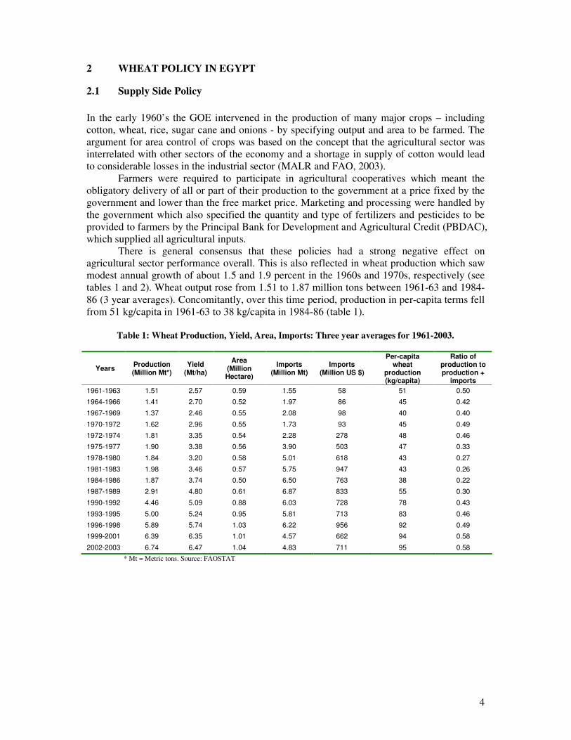
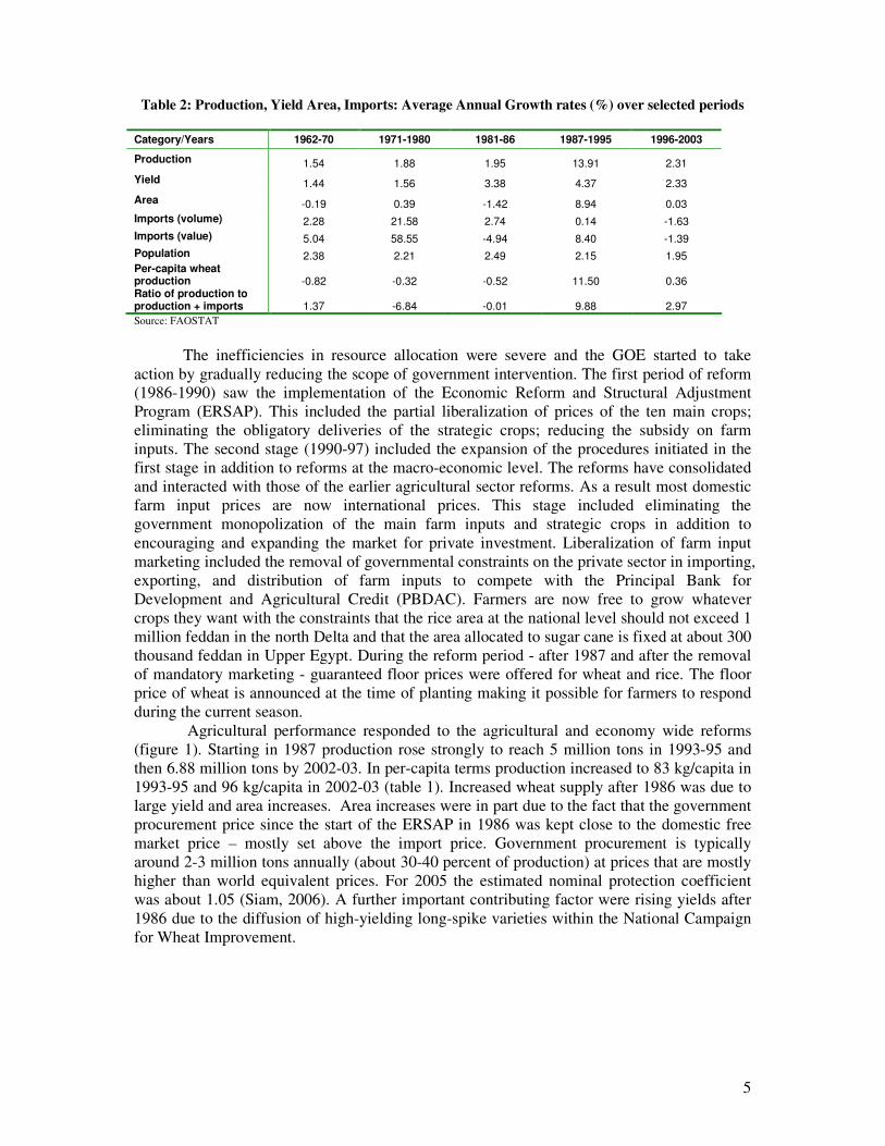
In the early 1960’s the GOE intervened in the production of many major crops – including cotton, wheat, rice, sugar cane and onions - by specifying output and area to be farmed. The argument for area control of crops was based on the concept that the agricultural sector was interrelated with other sectors of the economy and a shortage in supply of cotton would lead to considerable losses in the industrial sector (MALR and FAO, 2003). Farmers were required to participate in agricultural cooperatives which meant the obligatory delivery of all or part of their production to the government at a price fixed by the government and lower than the free market price. Marketing and processing were handled by the government which also specified the quantity and type of fertilizers and pesticides to be provided to farmers by the Principal Bank for Development and Agricultural Credit (PBDAC), which supplied all agricultural inputs. There is general consensus that these policies had a strong negative effect on agricultural sector performance overall. This is also reflected in wheat production which saw modest annual growth of about 1.5 and 1.9 percent in the 1960s and 1970s, respectively (see tables 1 and 2). Wheat output rose from 1.51 to 1.87 million tons between 1961-63 and 1984-86 (3 year averages). Concomitantly, over this time period, production in per-capita terms fell from 51 kg/capita in 1961-63 to 38 kg/capita in 1984-86 (table 1).

Table 1: Wheat Production, Yield, Area, Imports: Three year averages for 1961-2003.

Years Production (Million Mt*)

Yield (Mt/ha)

Area (Million Hectare)

Imports (Million Mt)

Imports (Million US $)

Per-capita wheat

production (kg/capita)

Ratio of production to production +

imports

1961-1963 1.51 2.57 0.59 1.55 58 51 0.50

1964-1966 1.41 2.70 0.52 1.97 86 45 0.42

1967-1969 1.37 2.46 0.55 2.08 98 40 0.40

1970-1972 1.62 2.96 0.55 1.73 93 45 0.49

1972-1974 1.81 3.35 0.54 2.28 278 48 0.46

1975-1977 1.90 3.38 0.56 3.90 503 47 0.33

1978-1980 1.84 3.20 0.58 5.01 618 43 0.27

1981-1983 1.98 3.46 0.57 5.75 947 43 0.26

1984-1986 1.87 3.74 0.50 6.50 763 38 0.22

1987-1989 2.91 4.80 0.61 6.87 833 55 0.30

1990-1992 4.46 5.09 0.88 6.03 728 78 0.43

1993-1995 5.00 5.24 0.95 5.81 713 83 0.46

1996-1998 5.89 5.74 1.03 6.22 956 92 0.49

1999-2001 6.39 6.35 1.01 4.57 662 94 0.58

2002-2003 6.74 6.47 1.04 4.83 711 95 0.58

* Mt = Metric tons. Source: FAOSTAT

5

Table 2: Production, Yield Area, Imports: Average Annual Growth rates (%) over selected periods

Category/Years 1962-70 1971-1980 1981-86 1987-1995 1996-2003

Production 1.54 1.88 1.95 13.91 2.31

Yield 1.44 1.56 3.38 4.37 2.33

Area -0.19 0.39 -1.42 8.94 0.03

Imports (volume) 2.28 21.58 2.74 0.14 -1.63

Imports (value) 5.04 58.55 -4.94 8.40 -1.39

Population 2.38 2.21 2.49 2.15 1.95 Per-capita wheat production -0.82 -0.32 -0.52 11.50 0.36 Ratio of production to production + imports 1.37 -6.84 -0.01 9.88 2.97

Source: FAOSTAT

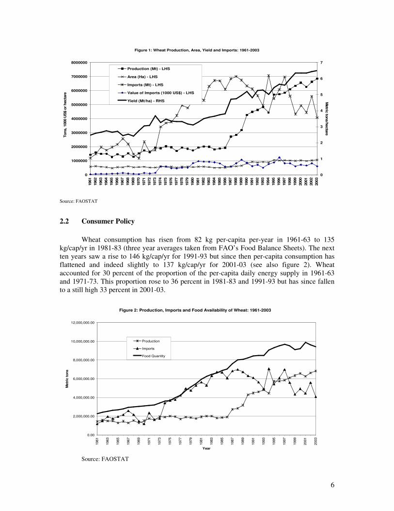
The inefficiencies in resource allocation were severe and the GOE started to take action by gradually reducing the scope of government intervention. The first period of reform (1986-1990) saw the implementation of the Economic Reform and Structural Adjustment Program (ERSAP). This included the partial liberalization of prices of the ten main crops; eliminating the obligatory deliveries of the strategic crops; reducing the subsidy on farm inputs. The second stage (1990-97) included the expansion of the procedures initiated in the first stage in addition to reforms at the macro-economic level. The reforms have consolidated and interacted with those of the earlier agricultural sector reforms. As a result most domestic farm input prices are now international prices. This stage included eliminating the government monopolization of the main farm inputs and strategic crops in addition to encouraging and expanding the market for private investment. Liberalization of farm input marketing included the removal of governmental constraints on the private sector in importing, exporting, and distribution of farm inputs to compete with the Principal Bank for Development and Agricultural Credit (PBDAC). Farmers are now free to grow whatever crops they want with the constraints that the rice area at the national level should not exceed 1 million feddan in the north Delta and that the area allocated to sugar cane is fixed at about 300 thousand feddan in Upper Egypt. During the reform period - after 1987 and after the removal of mandatory marketing - guaranteed floor prices were offered for wheat and rice. The floor price of wheat is announced at the time of planting making it possible for farmers to respond during the current season. Agricultural performance responded to the agricultural and economy wide reforms (figure 1). Starting in 1987 production rose strongly to reach 5 million tons in 1993-95 and then 6.88 million tons by 2002-03. In per-capita terms production increased to 83 kg/capita in 1993-95 and 96 kg/capita in 2002-03 (table 1). Increased wheat supply after 1986 was due to large yield and area increases. Area increases were in part due to the fact that the government procurement price since the start of the ERSAP in 1986 was kept close to the domestic free market price – mostly set above the import price. Government procurement is typically around 2-3 million tons annually (about 30-40 percent of production) at prices that are mostly higher than world equivalent prices. For 2005 the estimated nominal protection coefficient was about 1.05 (Siam, 2006). A further important contributing factor were rising yields after 1986 due to the diffusion of high-yielding long-spike varieties within the National Campaign for Wheat Improvement.

6

Figure 1: Wheat Production, Area, Yield and Imports: 1961-2003

0

1000000

2000000

3000000

4000000

5000000

6000000

7000000

8000000

1961

1962

1963

1964

1965

1966

1967

1968

1969

1970

1971

1972

1973

1974

1975

1976

1977

1978

1979

1980

1981

1982

1983

1984

1985

1986

1987

1988

1989

1990

1991

1992

1993

1994

1995

1996

1997

1998

1999

2000

2001

2002

2003

Tons, 1000 U

S$ o

r hecta

re

0

1

2

3

4

5

6

7

Metric

tons/h

ecta

reProduction (Mt) - LHS

Area (Ha) - LHS

Imports (Mt) - LHS

Value of Imports (1000 US$) - LHS

Yield (Mt/ha) - RHS

Source: FAOSTAT

2.2 Consumer Policy

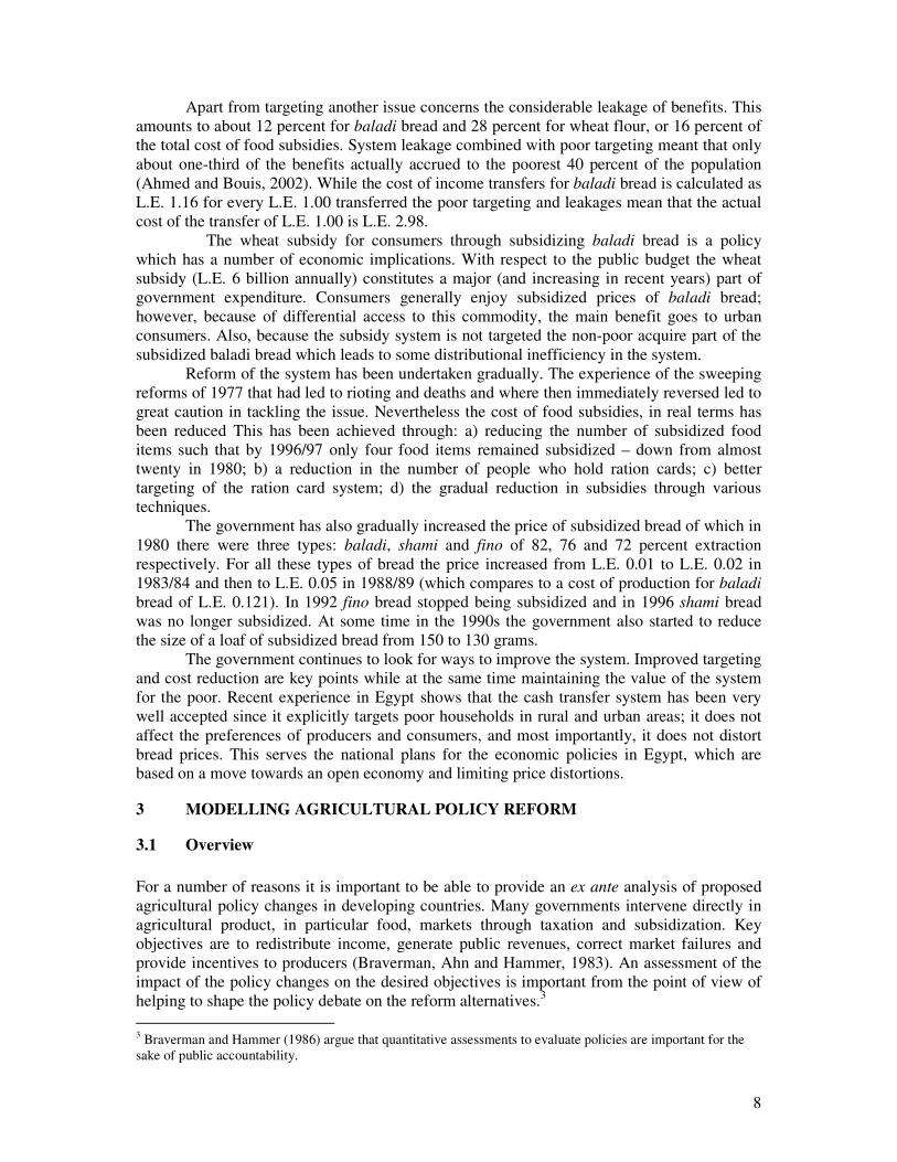
Wheat consumption has risen from 82 kg per-capita per-year in 1961-63 to 135 kg/cap/yr in 1981-83 (three year averages taken from FAO’s Food Balance Sheets). The next ten years saw a rise to 146 kg/cap/yr for 1991-93 but since then per-capita consumption has flattened and indeed slightly to 137 kg/cap/yr for 2001-03 (see also figure 2). Wheat accounted for 30 percent of the proportion of the per-capita daily energy supply in 1961-63 and 1971-73. This proportion rose to 36 percent in 1981-83 and 1991-93 but has since fallen to a still high 33 percent in 2001-03.

Figure 2: Production, Imports and Food Availability of Wheat: 1961-2003

0.00

2,000,000.00

4,000,000.00

6,000,000.00

8,000,000.00

10,000,000.00

12,000,000.00

1961

1963

1965

1967

1969

1971

1973

1975

1977

1979

1981

1983

1985

1987

1989

1991

1993

1995

1997

1999

2001

2003

Year

Metr

ic to

ns

Production

Imports

Food Quantity

Source: FAOSTAT

7

Wheat is the key staple food crop and the government’s food policy system can be seen as a reflection of its efforts to promote social equity and political stability. It’s roots can be traced to rising food prices after World War II which led to the GOE to become involved in importing large quantities of wheat and flour and selling them at a loss in government owned shops. The system of food subsidies continued to grow into an elaborate system of subsidies and rationing. Over time subsidized bread has become a powerful symbol of the broader social contract between the Egyptian government and the population (Ahmed et al, 2001). Subsidized wheat through baladi bread is about 6 million tons (for 2003) which constitute about 50 percent of the total consumption of wheat. Following the dramatic world price developments of the early 1970s Egypt’s food subsidies bill rose from 3 million Egyptian Pounds (L.E.) in 1970/71 to L.E. 1.4 billion in 1980/81 (Ahmed et al, 2001). Indeed, the early 1980s saw the unsustainable peak in subsidy expenditures which by then covered nearly 20 items.2 Despite a gradual reduction in the coverage to only four items – baladi bread, wheat flour, oil and sugar - the food subsidy system is still considered a major component of the social safety net (which also includes water, energy, housing, education, health and transportation) for the poor. It is credited with helping to reduce infant mortality and malnutrition (World Bank, 1995). In urban areas the baladi bread subsidy adds nearly 8 percent of total expenditure for the poorest 20 percent of households. For a number of reasons the food subsidy system has and continues to receive considerable attention. This is mainly because of the costliness of the system on the one hand and it’s political sensitivity on the other. The total subsidy for baladi bread and wheat flour represents about 5.1 percent of government expenditure (down from 14 percent in 1980/81) and about 1.3 percent of GDP for 2004/05. For baladi bread alone – and baladi bread accounts for about 60 percent of the total (with another 15 percent accounted for by wheat flour) - the cost of the subsidy was about L.E. 6 billion in 2004 (Siam (2006)). However, Adams (2000) notes that subsidies on water and electricity incur a significantly higher cost to the government than do food subsidies (even without including rural areas in his calculations – as data is difficult to obtain). Food receives more attention also because in the case of wheat it adds significantly to the import bill and thus has an impact on the external debt of the country and the balance of payments. Egypt is consistently one of the world’s largest (top ten) wheat importers with a wheat import bill averaging 711 million US $ in 2002-03 (table 1). A number of important issues continue to be of concern to policy makers. One is that of targeting. With regard to baladi bread all households have equal access and about 75 percent of the non-poor and 66 percent of the poor receive subsidized bread. The per-capita monthly benefit to consumers from baladi bread is quite evenly distributed across income groups and this is especially true for rural areas. In effect 1 percent of the population receive more or less 1 percent of the subsidy benefits, regardless of their income level (Ahmed et al, 2001). While in principle access is equal in reality the location of bakeries means that Egyptians living in rural areas – about 58 percent of the total - receive only 30 percent of the total food subsidies in 1996/97. Apart from this bias the self-targeting nature means that in urban areas where baladi bread is considered an inferior good, the urban poor receive more in terms of income transfers from the food subsidies than the rich. In rural areas baladi bread is not an inferior good and only baladi wheat flour is consumed more in absolute terms by the poor. Overall Ahmed et al (2001) find that the poor benefit slightly less than the rich from income transfers (see also Adams, 2000).

2 For more detail on the evolution and description of the food subsidy system see Gutner (1999), Ahmed et al (2001) and Kherallah et al (2000).

8

Apart from targeting another issue concerns the considerable leakage of benefits. This amounts to about 12 percent for baladi bread and 28 percent for wheat flour, or 16 percent of the total cost of food subsidies. System leakage combined with poor targeting meant that only about one-third of the benefits actually accrued to the poorest 40 percent of the population (Ahmed and Bouis, 2002). While the cost of income transfers for baladi bread is calculated as L.E. 1.16 for every L.E. 1.00 transferred the poor targeting and leakages mean that the actual cost of the transfer of L.E. 1.00 is L.E. 2.98. The wheat subsidy for consumers through subsidizing baladi bread is a policy which has a number of economic implications. With respect to the public budget the wheat subsidy (L.E. 6 billion annually) constitutes a major (and increasing in recent years) part of government expenditure. Consumers generally enjoy subsidized prices of baladi bread; however, because of differential access to this commodity, the main benefit goes to urban consumers. Also, because the subsidy system is not targeted the non-poor acquire part of the subsidized baladi bread which leads to some distributional inefficiency in the system. Reform of the system has been undertaken gradually. The experience of the sweeping reforms of 1977 that had led to rioting and deaths and where then immediately reversed led to great caution in tackling the issue. Nevertheless the cost of food subsidies, in real terms has been reduced This has been achieved through: a) reducing the number of subsidized food items such that by 1996/97 only four food items remained subsidized – down from almost twenty in 1980; b) a reduction in the number of people who hold ration cards; c) better targeting of the ration card system; d) the gradual reduction in subsidies through various techniques. The government has also gradually increased the price of subsidized bread of which in 1980 there were three types: baladi, shami and fino of 82, 76 and 72 percent extraction respectively. For all these types of bread the price increased from L.E. 0.01 to L.E. 0.02 in 1983/84 and then to L.E. 0.05 in 1988/89 (which compares to a cost of production for baladi bread of L.E. 0.121). In 1992 fino bread stopped being subsidized and in 1996 shami bread was no longer subsidized. At some time in the 1990s the government also started to reduce the size of a loaf of subsidized bread from 150 to 130 grams. The government continues to look for ways to improve the system. Improved targeting and cost reduction are key points while at the same time maintaining the value of the system for the poor. Recent experience in Egypt shows that the cash transfer system has been very well accepted since it explicitly targets poor households in rural and urban areas; it does not affect the preferences of producers and consumers, and most importantly, it does not distort bread prices. This serves the national plans for the economic policies in Egypt, which are based on a move towards an open economy and limiting price distortions.

3 MODELLING AGRICULTURAL POLICY REFORM

3.1 Overview

For a number of reasons it is important to be able to provide an ex ante analysis of proposed agricultural policy changes in developing countries. Many governments intervene directly in agricultural product, in particular food, markets through taxation and subsidization. Key objectives are to redistribute income, generate public revenues, correct market failures and provide incentives to producers (Braverman, Ahn and Hammer, 1983). An assessment of the impact of the policy changes on the desired objectives is important from the point of view of helping to shape the policy debate on the reform alternatives.3

3 Braverman and Hammer (1986) argue that quantitative assessments to evaluate policies are important for the sake of public accountability.

9

Starting in the 1990s, the focus shifted to poverty and hunger reduction. These issues are still predominantly rural based: the rural poor make up about 70 percent of the world’s total poor population. Nevertheless, urbanisation processes have recently increased the number of urban poor and food insecure. Increasingly, therefore, the role of agricultural based growth in promoting rural development, slowing down the pace of urbanisation and contributing to an equitable and sustainable overall development is recognised and emphasised. A focus on the welfare of the rural population and its interdependencies with the welfare of urban areas, as well as the interlinkages between agricultural and off-farm activities is essential to foster greater understanding of the links between agricultural policies, rural development and poverty and food insecurity. In this study we apply one tool that has been used to analyze ex ante the impact of agricultural policy reforms, i.e. a multi-market model. Discussion of other types of measures and models is limited to a brief comparison.4 The most commonly used tool to quantitatively assess agricultural pricing policies are the domestic resource cost (DRC) and the effective protection rate (EPR). Both are modified ratios of domestic prices to international prices, the latter assumed as efficiency benchmarks for the domestic economy. These measures are often calculated at different levels of the value chain of specific commodities and reported as summary indicators of the so called “Policy Analysis Matrix” (PAM) (Monke and Pearson, 1989). These measures can only partially address the issues of interest outlined above. In particular income distribution, public revenue and the impact of taxes or subsidies on production and consumption are not evaluated by such measures. Another popular method is that of single-market calculations of consumers’ and producers’ surplus. This type of analysis ignores the interaction among markets, i.e. substitution effects in consumption and production, and provides only limited information with regard to income distribution. The rural labor market is not included and hence the potentially important direct and indirect effects on wages are ignored. Ignoring the direct and indirect effects on wages, prices and incomes means that the estimates of welfare changes will be biased in unknown directions (Arulpragasam and Conway, 2003). The most sophisticated solution to incorporating direct and indirect effects in several markets has been to prepare computable general equilibrium models (CGE). These model goods and factors markets in all sectors and allow for wages, prices and incomes to be determined endogenously. The main drawbacks of these types of models are their large data requirements and their high degree of complexity.5

3.2 Multi-market models6

Multi-market models fall short of the complexity of CGEs but do include direct and indirect effects in a small number of markets. In that sense they are an improvement over single market partial equilibrium analysis. They typically consist of a producer and consumer core and allow for the analysis of the impact of price and non-price policies on production, factor use, prices (for non-tradables), incomes, consumption, government revenues and expenditures and balance of trade (Sadoulet and de Janvry, 1995). The analysis focuses on those markets which are assumed to be strongly interlinked, either on the demand or the supply side. Prices in those markets included in the analysis are endogenous. The bias in estimating welfare changes as a result of policy reforms is diminished, but remains. It follows that multi-market

4 A more detailed discussion of the various tools to analyse policy change can be found in World Bank (2003). 5 For a somewhat more detailed exposition on the DRC, EPR and CGE models see Sadoulet and de Janvry (1995). 6 Multi-market models are sometimes referred to as “limited general equilibrium” (for example in Quizón and Binswanger, 1986) or “multi-market partial equilibrium” (as in Arulpragasam and Conway, 2003) models.

10

models will generate reliable results when the reforms being analysed affect commodities or factors for which the set of close substitutes and complements are well defined (Arulpragasam and Conway, 2003). Multi-market models have proven particularly popular for work on agriculture sector analysis. In the 1980s the World Bank developed multi-market models for Senegal, South Korea and Cyprus to analyse how the impact of changes in price policies would affect production, demand, income, trade and government revenues (Lundberg and Rich, 2002). Braverman, Ahn and Hammer (1983) and Braverman and Hammer (1986) extended the single market surplus method to include income distribution and some general equilibrium considerations. Their analyses cover the agricultural sector and includes an exogenous urban sector.7 This is important as urban consumption may have an important impact on government revenue/deficits. Moreover staple food price changes are important for the urban poor. They note the trade-off between complete information on the consequences of policy and the need for simplicity in operational work. Braverman, Ahn and Hammer (1983) use a multi-market model to evaluate quantitatively the impact of alternative pricing policies aimed at reducing the deficits in the Grain Management Fund and the Fertilizer Fund in Korea. In particular they measure the impact of the various alternatives on: i) Production and consumption of rice and barley, ii) real income distribution, including the income distribution in both rural and urban sectors, iii) import levels of rice, iv) self-sufficiency in rice and v) the public budget. On the supply side Braverman and Hammer (1986) assume a Cobb-Douglas technology. Land and labor are fixed to the region but can be shifted between crops within the region. Their allocation is determined by equating their value marginal products between uses. Incomes are determined by profits and non-agricultural receipts held exogenous. The analysis of demand is based on the Almost Ideal Demand System (AIDS). Quizón and Binswanger (1986) use a multi-market model to analyse the impact of agricultural policies as well as technical and economic changes on growth and equity in India. Their model covered four outputs and three inputs, including labor. Households are divided by income into four urban and four rural groups. They note that the distributional outcomes from general equilibrium models depend crucially on labor market assumptions.8 Accurate modelling of wage formation is therefore central to obtaining meaningful results. More recently multi-market models have been used for agricultural sector Poverty and Social Impact Analysis (PSIA).9 Murembya (1998) uses a multi-market model along the lines of Braverman and Hammer (1986) to study the impact of loosening agricultural price controls on agricultural production in the smallholder sector, the government budget deficit and on household welfare in Malawi. Dorosh and Bernier (1994) construct a multi-market model in the tradition of Braverman and Hammer (1986) that includes yellow and white maize, rice, wheat and bread, export crops and vegetables, meat and non-agriculture. For vegetables and meat trade is thin and is fixed exogenously in the model. Three household groups are included: urban poor, urban non-poor and rural. Demand side parameters are estimated using an AIDS model while supply side elasticities are based mainly on data from other countries. Dorosh et al (1995) addresses the question of whether open market sales of yellow maize food aid is an effective means of poverty alleviation in Maputo and whether such a policy has any negative effects on the rural poor.

7 Lau et al (1981) is an earlier example of an application of the farm household model in a policy simulation study. They did not include the urban sector. 8 Quoting Taylor (1979). 9 For detailed information on PSIA see the so dedicated World Bank website [ www.worldbank.org/psia ]. For a detailed overview of analyses on agricultural market reforms on poverty and welfare see Lundberg (2005).

11

Minot and Goletti (1998) use a spatial multi-market analysis which focuses on market liberalization of the rice sector in Vietnam.10 Their model is innovative in the sense that it allows for differences in impact across regions. Building on their work (and also using the Viet Nam Agricultural Spatial-Equilibrium Model) Goletti and Rich (1998a) study alternative policy options for agricultural diversification in Viet Nam and Goletti and Rich (1998b) use the Madagascar multi-market spatial-equilibrium model to analyse agricultural policy options for poverty reduction. Srinivasan and Jha (2001) analyze the effect of liberalizing foodgrain trade on domestic price stability using a multi-market model. In their model the direction of trade is determined endogenously. Lundberg and Rich (2002) built a multi-market model to look at agricultural reforms in Madagascar. This was meant to be a generic model that could be adapted to policy analysis in a number of African countries. On the product side this model includes fine and coarse grains, roots and tubers, cash crops, livestock, other food products and non-agricultural production. On the input side fertilizer, feed and land were included. Labor was not included as the authors surmised that this input was more appropriately studied through the use of a CGE model. Stifel and Randrianarisoa (2004) built on Lundberg and Rich (2002) and included a seasonal dimension to analyze the impact of agricultural reforms, such as tariff changes, but also going beyond price changes by looking at infrastructure improvements and yield increases, in Madagascar.

4 THE EGYPT MULTI-MARKET MODEL

4.1 Product categories

The product categories are: 1) food items, 2) non-food items, 3) animal-feed commodities, and; 4) agricultural inputs. More specifically, these items include: Wheat (both subsidized and un-subsidized): Wheat is the backbone of the food security policy in Egypt. About half of the total consumption of wheat is baladi bread which is subject to subsidy. Subsidized baladi bread it treated as autonomous wheat consumption, i.e. independent of market prices. Consumer demand is taken as demand for un-subsidized wheat which is a function of prices and income but is conditional on the level of subsidized wheat. Maize: This product is the second cereal crop after wheat in terms of cultivated area. It competes with rice and cotton as well as some other summer crops. Locally produced maize is used partially for food and partially for animal feed. Imported maize is used as feed in poultry production. We include maize twice, once the maize used for human consumption and once for animal consumption. To simplify the model prices are assumed to be linked and identical for locally produced and imported maize. Rice: Rice is the only exportable cereal crop and it is the third crop after wheat and maize in terms of cultivated area. While cotton declined rice cultivation expanded, encouraged also by incentives to wheat as the two crops are complementary in the crop rotation. Rice cultivation is very water intensive and uses about 20 percent of the total water used by agriculture which explains why, in theory, the area cultivated to rice is meant to be restricted. Yet free water subsidizes rice the most. Berseem: This product (Egyptian clover) is used entirely as animal feed. It is non-tradable. Cotton: Cotton is the major non-food cash crop in Egypt that also contributes the largest share to the value of the country’s agricultural exports. It is a summer crop that is

10 See also Minot and Goletti (2000).

12

usually grown after short-season berseem so while it is complementary to short season berseem it competes with both wheat and long-season berseem as well as with summer crops. Around 60-70 percent of domestic production is used as an input to the local cotton industry and the remainder is exported. In this study we assume that industry demand for cotton represents the final demand. Livestock (meat): Livestock production contributes about one third of the value added originating in agriculture. Meat and dairy are the main products of this sub-sector. In this study, we assume that livestock production is only for meat. Onions: Included as representative of vegetable commodities with export potential. Dry onions were the sixth most important agricultural export commodity in 2004, by value. Oranges: Included as representative of fruits with export potential. Oranges were the third most valuable agricultural export item in 2004. Potatoes: This product is the key starchy root product with significant domestic consumption as well as being an important export crop (4th most valuable agricultural export item in 2004). Two agricultural inputs are modelled explicitly: Fertilizer: This covers the main fertilizer used, nitrogen. Fertilizer consumption levels are based on recommended use levels (from FAO, 2005) for the crops included. Supply of fertilizer is assumed exogenous. It is treated as a tradable commodity. Mechanical traction: This is the number of tractors in use (from FAOSTAT). At the household level traction use is based on the value of farm equipment (excluding water pumps) owned by household group and is obtained from the Egypt Integrated Household Survey (more details given below in section 4). It is treated as a non-tradable commodity. Land, labor and water: Land is included as a variable input but is not incorporated into the model as a traded commodity. The land shares are restricted to sum to 1 or more. Labor and water are included in the model through fixed coefficients and their respective levels are derived from the level of land allocated to a particular crop.11

4.2 Households

Production and consumption patterns are distinguished among nine broad types of household groups: urban top, urban middle, urban bottom, rural non-farming top, rural non-farming middle, rural non-farming bottom, rural farming top, rural farming middle, rural farming bottom. Where top, middle and bottom refer to the top 20 percent, the middle 50 percent and the bottom 30 percent of households on the basis of per-capita income. Only rural farming households are involved in agricultural production activities.

4.3 Structure of the model

The multi-market model is an adaptation of Stifel and Randrianarisoa (2004) and consists of six blocks of equations: prices, supply, input demand, consumption, income and equilibrium conditions.12 Unlike Stifel and Randrianarisoa (2004) we do not include seasonality nor an aggregate for all other food as well as non-food commodities in the model. Below we detail the different sets of equations, present the data used and explain which are their sources. Prices: Consumer prices (PC) are higher than producer prices (PP) due to the domestic marketing margin (MARG) which can proxy, for example transportation costs due

11 Water and Labor coefficients are taken from Nassar and Khaireldin, 2005, "Cropping pattern alternatives for Egypt," mimeo, Center for Agricultural Economic Studies, Cairo University. 12 The model described below is different to the one used in Siam (2006) but generates broadly similar results.

13

to infrastructure improvements. A possible subsidy to producer prices is allowed for by including PSUB.

( ) )1(1)1( ,,,,, crcrhcrhc PSUBMARGPPPC −•+•=

where the subscripts c, h, and r refer to commodity, household type and region, respectively. The border price (PM) of the importable products (im) wheat and maize are linked to the world price by the exchange rate (er), import tariffs (tm), and the international marketing margin (RMARG).

)2()1()1( imimimim tmRMARGerPWPM +•+••=

The border price (PX) of the exportable products (ix) rice, onions, cotton and fertilizer13 are linked to the world price by the exchange rate (er), import tariffs (tm), and the international marketing margin (RMARG).

( ) ( )( )3

11 ixix

ixix

teRMARG

erPWPX

+•+

•=

Consumer prices for the importable items are related to the border price by the commodity specific border-to-market marketing margin and by a possible consumer subsidy (CSUB):

( ) )4(1)1('', imimimurbanim CSUBIMARGPMPC −•+•=

where IMARG is the border-to-market marketing margin, specific to commodities. Consumer prices for the exportable items are related to the border price by the commodity specific market-to-border marketing margin:

)5(1(

)1('',

ix

ixixurbanim

IMARG

MARGPXPC

+

+•=

where IMARG is the market-to-border marketing margin, specific to commodities. Rural consumer prices differ from urban consumer prices by an internal marketing margin (INTMARG) that reflects transportation and marketing costs.

)6()1('','', cruralcurbanc INTMARGPCPC +•=

The internal marketing margin is positive for products which are primarily exported from rural to urban areas. Products that are assumed not to move from rural to urban or vice-versa have a zero INTMARG). This particular set-up allows one to distinguish between farm to rural (MARG), rural to urban (INTMARG) and urban to border (IMARG). We assume that households in the different income groups face the same prices but that these vary by region. We include a price index for each household group to reflect changes in prices weighted by their shares of consumption:

13 Oranges and potatoes are also exported in sizeable quantities but it is assumed that domestic demand determines their price. We return to this issue in the section on the equilibrium conditions.

14

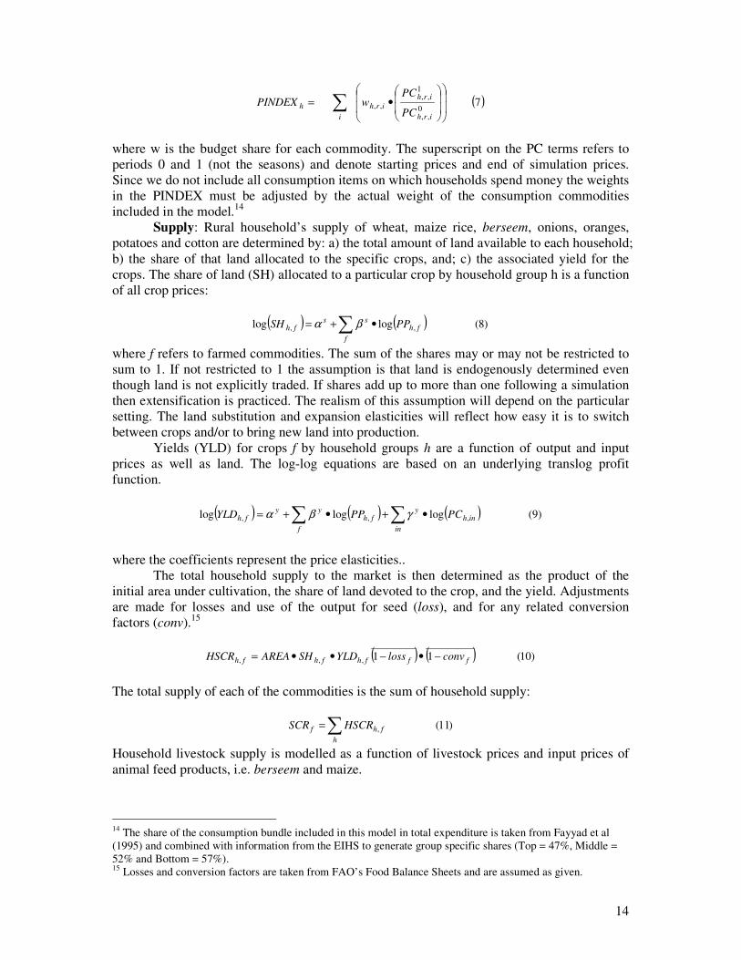
( )70

,,

1,,

,,

•= ∑

irh

irh

irh

i

hPC

PCwPINDEX

where w is the budget share for each commodity. The superscript on the PC terms refers to periods 0 and 1 (not the seasons) and denote starting prices and end of simulation prices. Since we do not include all consumption items on which households spend money the weights in the PINDEX must be adjusted by the actual weight of the consumption commodities included in the model.14 Supply: Rural household’s supply of wheat, maize rice, berseem, onions, oranges, potatoes and cotton are determined by: a) the total amount of land available to each household; b) the share of that land allocated to the specific crops, and; c) the associated yield for the crops. The share of land (SH) allocated to a particular crop by household group h is a function of all crop prices:

( ) ( ) )8(loglog ,, fh

f

ssfh PPSH •+= ∑ βα

where f refers to farmed commodities. The sum of the shares may or may not be restricted to sum to 1. If not restricted to 1 the assumption is that land is endogenously determined even though land is not explicitly traded. If shares add up to more than one following a simulation then extensification is practiced. The realism of this assumption will depend on the particular setting. The land substitution and expansion elasticities will reflect how easy it is to switch between crops and/or to bring new land into production. Yields (YLD) for crops f by household groups h are a function of output and input prices as well as land. The log-log equations are based on an underlying translog profit function.

( ) ( ) ( ) )9(logloglog ,,, inh

in

yfh

f

yyfh PCPPYLD •+•+= ∑∑ γβα

where the coefficients represent the price elasticities.. The total household supply to the market is then determined as the product of the initial area under cultivation, the share of land devoted to the crop, and the yield. Adjustments are made for losses and use of the output for seed (loss), and for any related conversion factors (conv).15

( ) ( ) )10(11,,, fffhfhfh convlossYLDSHAREAHSCR −•−••=

The total supply of each of the commodities is the sum of household supply:

)11(,∑=h

fhf HSCRSCR

Household livestock supply is modelled as a function of livestock prices and input prices of animal feed products, i.e. berseem and maize.

14 The share of the consumption bundle included in this model in total expenditure is taken from Fayyad et al (1995) and combined with information from the EIHS to generate group specific shares (Top = 47%, Middle = 52% and Bottom = 57%). 15 Losses and conversion factors are taken from FAO’s Food Balance Sheets and are assumed as given.

15

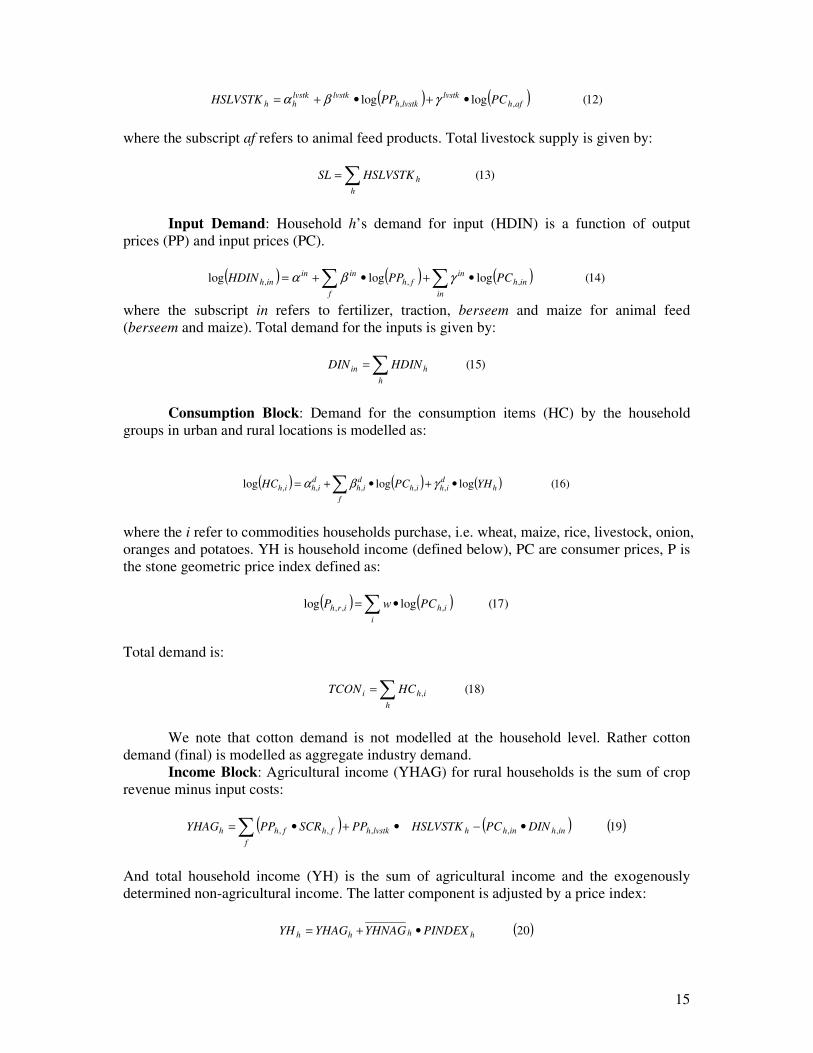
( ) ( ) )12(loglog ,, afhlvstk

lvstkhlvstklvstk

hh PCPPHSLVSTK •+•+= γβα

where the subscript af refers to animal feed products. Total livestock supply is given by:

)13(∑=h

hHSLVSTKSL

Input Demand: Household h’s demand for input (HDIN) is a function of output prices (PP) and input prices (PC).

( ) ( ) ( ) )14(logloglog ,,, inh

in

infh

f

inininh PCPPHDIN •+•+= ∑∑ γβα

where the subscript in refers to fertilizer, traction, berseem and maize for animal feed (berseem and maize). Total demand for the inputs is given by:

)15(∑=

h

hin HDINDIN

Consumption Block: Demand for the consumption items (HC) by the household groups in urban and rural locations is modelled as:

( ) ( ) ( ) )16(logloglog ,,,,, hd

ihih

f

dih

dihih YHPCHC •+•+= ∑ γβα

where the i refer to commodities households purchase, i.e. wheat, maize, rice, livestock, onion, oranges and potatoes. YH is household income (defined below), PC are consumer prices, P is the stone geometric price index defined as:

( ) ( ) )17(loglog ,,, ∑ •=i

ihirh PCwP

Total demand is:

)18(,∑=

h

ihi HCTCON

We note that cotton demand is not modelled at the household level. Rather cotton demand (final) is modelled as aggregate industry demand. Income Block: Agricultural income (YHAG) for rural households is the sum of crop revenue minus input costs:

( ) ( ) ( )19,,,,, inhinhhlvstkh

f

fhfhh DINPCHSLVSTKPPSCRPPYHAG •−•+•=∑

And total household income (YH) is the sum of agricultural income and the exogenously determined non-agricultural income. The latter component is adjusted by a price index:

( )20hhhh PINDEXYHNAGYHAGYH •+=

16

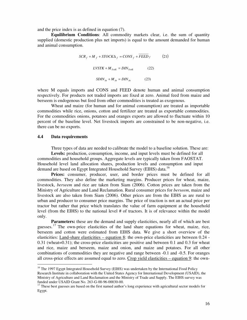
and the price index is as defined in equation (7). Equilibrium Conditions: All commodity markets clear, i.e. the sum of quantity supplied (domestic production plus net imports) is equal to the amount demanded for human and animal consumption.

( )21fffff FEEDCONSSTOCKMSCR +=∆++

)22(lvstklvstk DINMLVSTK =+

)23(ininin DINMSDIN =+

where M equals imports and CONS and FEED denote human and animal consumption respectively. For products not traded imports are fixed at zero. Animal feed from maize and berseem is endogenous but feed from other commodities is treated as exogenous. Wheat and maize (for human and for animal consumption) are treated as importable commodities while rice, onions, cotton and fertilizer are treated as exportable commodities. For the commodities onions, potatoes and oranges exports are allowed to fluctuate within 10 percent of the baseline level. Net livestock imports are constrained to be non-negative, i.e. there can be no exports.

4.4 Data requirements

Three types of data are needed to calibrate the model to a baseline solution. These are: Levels: production, consumption, income, and input levels must be defined for all commodities and household groups. Aggregate levels are typically taken from FAOSTAT. Household level land allocation shares, production levels and consumption and input demand are based on Egypt Integrated Household Survey (EIHS) data.16 Prices: consumer, producer, user, and border prices must be defined for all commodities. They also define the marketing margins. Producer prices for wheat, maize, livestock, berseem and rice are taken from Siam (2006). Cotton prices are taken from the Ministry of Agriculture and Land Reclamation. Rural consumer prices for berseem, maize and livestock are also taken from Siam (2006). Other prices are from the EIHS as are rural to urban and producer to consumer price margins. The price of traction is not an actual price per tractor but rather that price which translates the value of farm equipment at the household level (from the EIHS) to the national level # of tractors. It is of relevance within the model only. Parameters: these are the demand and supply elasticities, nearly all of which are best guesses. 17 The own-price elasticities of the land share equations for wheat, maize, rice, berseem and cotton were estimated from EIHS data. We give a short overview of the elasticities: Land-share elasticities – equation 8: the own-price elasticities are between 0.24 - 0.31 (wheat=0.31); the cross-price elasticities are positive and between 0.1 and 0.3 for wheat and rice, maize and berseem, maize and onion, and maize and potatoes. For all other combinations of commodities they are negative and range between -0.1 and -0.5. For oranges all cross-price effects are assumed equal to zero. Crop yield elasticities – equation 9: the own-

16 The 1997 Egypt Integrated Household Survey (EIHS) was undertaken by the International Food Policy Research Institute in collaboration with the United States Agency for International Development (USAID), the Ministry of Agriculture and Land Reclamation and the Ministry of Trade and Supply. The EIHS survey was funded under USAID Grant No. 263-G-00-96-00030-00. 17 These best guesses are based on the first named author’s long experience with agricultural sector models for Egypt.

17

price elasticities are between 0.3 and 0.5 (0.4 for wheat) except for cotton which is 1.2. The cross-price elasticities are all assumed equal to zero. Crop yield elasticities with respect to input prices are -0.7 for fertilizer and -0.9 for traction (in line with Antle and Aitah’s (1986) results for maize, rice and cotton). Livestock output supply elasticities – equation 12: The own-price elasticity is 0.6 and the elasticity of livestock supply with regard to animal feed prices are -0.5 for both maize and berseem. Input demand elasticities – equation 14: The own-price elasticity for fertilizer and animal-feed maize is -0.4 and for traction and berseem it is -0.5. The price elasticities of fertilizer and traction with regard to the price of the crop to which they are applied is 0.1 for all crops except for berseem for which it is 0.05 (for traction). All cross-price effects are assumed to be zero. The elasticities for animal-feed maize and berseem with respect to livestock price is 0.2 and 0.7 respectively. The cross-price effects for the two animal feed products is 0.2. Consumer demand elasticities – equation 16: The own price demand elasticity -0.3 for all commodities except for maize for which it is -0.2 and livestock for which it is -0.7. Cross-price effects are between -0.1 and -0.3 except for wheat and rice for which it is 0.2. Demand elasticities with respect to income are -0.1 for wheat and maize, 0.1 for rice, onion, oranges and potatoes and 0.2 for livestock. Demand for cotton is modeled separately as aggregate industry demand with a own price elasticity of 0.5. An assessment of the sensitivity of the model results with regard to the parameters is given in section 5.1.1

4.5 Baseline solution18

The baseline solution corresponds to wheat production of 5.5 million tons per year. This corresponds to 2.5 million feddan of land, and about 4 billion m3 of water, and imports of 5.2 million tons of wheat per year. Total availability, including imports, losses and animal feed is about 10.7 million tons. The subsidized producer and urban and rural consumer prices are 1,175, 1,507 and 1,117 L.E./ton whereas the respective unsubsidized prices are 1,056, 2,412 and 1,788 L.E./ton. The combined producer and consumer subsidy is estimated as 7.9 billion L.E. This figure is based on the assumptions with regard to quantities and prices made for this model and is appropriate for comparisons among the baseline and scenarios. It is not necessarily accurate in an absolute sense.

Berseem, as a winter crop, is highly competitive with wheat (cultivated on a similar amount of land). Production is over 65 million tons a year, all for local consumption, and there are no imports. Wheat, maize, rice, berseem and cotton account for 26, 20, 15, 29 and 6 percent of total land where total land is the sum of land cultivated to the eight commodities included in the system. Finally, caloric intake levels are calculated on the basis of calorie conversion factors based on the FAO Food Balance Sheets.

5 POLICY SIMULATION RESULTS

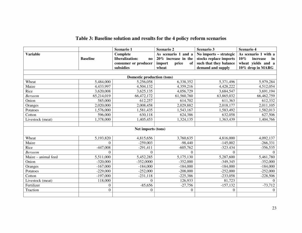
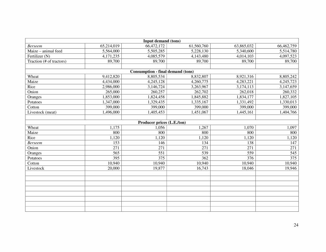
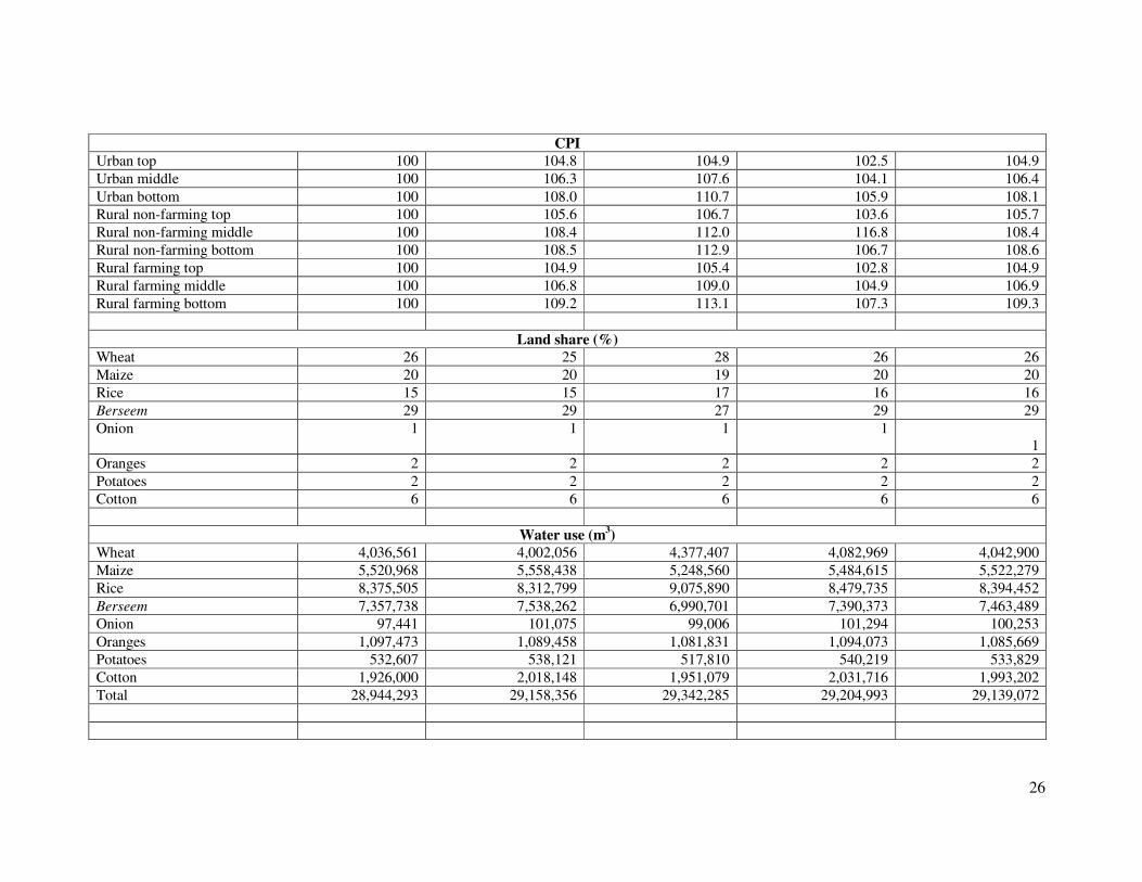
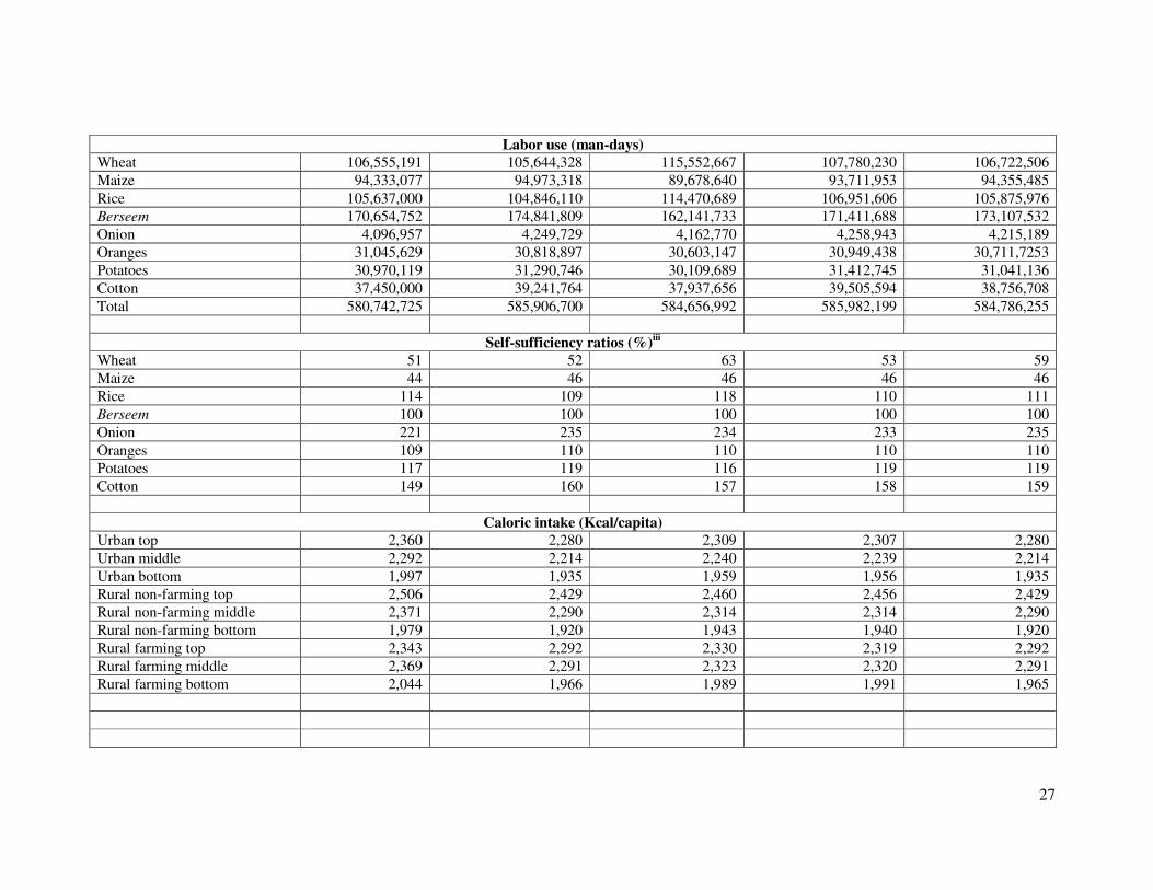
Four policy scenarios are analyzed using the multi-market model: 1) Complete liberalization; 2) increasing the import price of wheat by 20 percent; 3) replacing imports with strategic stocks; 4) increasing wheat yields by 10 percent accompanied by a reduction in marketing costs of 10 percent. Results are shown in table 3.

18 The baseline data set is calibrated using interlinked excel sheets that may be useful to others [even if considerable adaptation will inevitably be required] in simplifying this kind of exercise. The excel file for this Egypt multi-market baseline is available from André Croppenstedt at andre.croppenstedt@fao.org.

18

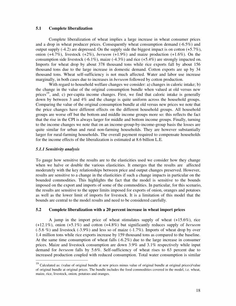
5.1 Complete liberalization

Complete liberalization of wheat implies a large increase in wheat consumer prices and a drop in wheat producer prices. Consequently wheat consumption demand (-6.5%) and output supply (-4.2) are depressed. On the supply side the biggest impact is on cotton (+5.7%), onion (+4.7%), livestock (+2%), berseem (+1.9%) and maize production (+1.6%). On the consumption side livestock (-6.1%), maize (-4.3%) and rice (+5.4%) are strongly impacted on. Imports for wheat drop by about 378 thousand tons while rice exports fall by about 156 thousand tons due to the large increase in domestic demand. Cotton exports are up by 34 thousand tons. Wheat self-sufficiency is not much affected. Water and labor use increase marginally, in both cases due to increases in berseem followed by cotton production. With regard to household welfare changes we consider: a) changes in caloric intake; b) the change in the value of the original consumption bundle when valued at old versus new prices19, and; c) per-capita income changes. First, we find that caloric intake is generally down by between 3 and 4% and the change is quite uniform across the household groups. Comparing the value of the original consumption bundle at old versus new prices we note that the price changes have different effects on the different household groups. All household groups are worse off but the bottom and middle income groups more so: this reflects the fact that the rise in the CPI is always larger for middle and bottom income groups. Finally, turning to the income changes we note that on an income-group-by-income-group basis the losses are quite similar for urban and rural non-farming households. They are however substantially larger for rural-farming households. The overall payment required to compensate households for the income effects of the liberalization is estimated at 8.6 billion L.E.

5.1.1 Sensitivity analysis

To gauge how sensitive the results are to the elasticities used we consider how they change when we halve or double the various elasticities. It emerges that the results are affected moderately with the key relationships between price and output changes preserved. However, results are sensitive to a change in the elasticities if such a change impacts in particular on the bounded commodities. This highlights the fact that the model is sensitive to the bounds imposed on the export and imports of some of the commodities. In particular, for this scenario, the results are sensitive to the upper limits imposed for exports of onion, oranges and potatoes as well as the lower limit of imports for livestock. It is a limitation of this model that the bounds are central to the model results and need to be considered carefully.

5.2 Complete liberalization with a 20 percent increase in wheat import prices

A jump in the import price of wheat stimulates supply of wheat (+15.6%), rice (+12.1%), onion (+5.1%) and cotton (+4.8%) but significantly reduces supply of berseem (-5.6 %) and livestock (-3.9%) and less so of maize (-1.7%). Imports of wheat drop by over 1.4 million tons while rice exports increase by 159 thousand tons as compared to the baseline. At the same time consumption of wheat falls (-6.2%) due to the large increase in consumer prices. Maize and livestock consumption are down 3.9% and 3.1% respectively while input demand for berseem falls by 5.6%. Self-sufficiency of wheat rises to 63 percent due to increased production coupled with reduced consumption. Total water consumption is similar 19 Calculated as: (value of original bundle at new prices minus value of original bundle at original prices)/value

of original bundle at original prices. The bundle includes the food commodities covered in the model, i.e. wheat, maize, rice, livestock, onion, potatoes and oranges.

19

to that found for scenario 1 but the increase over the baseline is now mainly due to increased water use for rice and to a lesser extent wheat. Labor use is a little lower than in scenario 1 with the increase over the baseline due, more or less equally, to wheat and rice. The implied price increases as measured by the CPI are relatively large and, except for the top income group for which livestock represents a relatively larger proportion of consumption, larger than for scenario 1. Caloric intake falls but the impact is weaker than in scenario 1. The difference lies in part in the greater responsiveness of rice consumption and the smaller fall in livestock consumption combined with the more moderate reductions in the consumption of the other commodities. Moreover although the wheat prices increase more livestock prices fall quite strongly in this scenario. The change in the value of the original consumption bundle from old to new prices shows that the urban top group is better off while for the rural farming top the change is neutral. For urban middle and rural non-farming top the change is very small. Most severely affected are rural non-farming middle, followed by rural farming bottom and rural non-farming bottom. The impact is much milder than in scenario 1 due to the larger shift to rice consumption and the larger fall in particular of consumer livestock prices (and livestock weighing more heavily in consumption the higher the income). The per-capita income changes are negative for all households and are in the range of 5 to 20 percent. In all regions the middle and bottom groups are worst affected. The rural farming households are again worst affected by this measure with both middle and bottom groups being significantly worse off than the top group which itself sees per-capita income fall by 13.5 percent. The overall payment required to compensate households for the income effects of the liberalization is estimated at 26.8 billion L.E.

5.3 Substituting imports with strategic stocks

Sudden upward shocks to the world price of wheat can be mitigated through the use of strategic stocks (replacing imports). Not surprisingly, because the level of strategic stocks chosen coincides with the level of imports for scenario 1, the implied production and consumption changes are similar to scenario 1. The benefit to households, both urban and rural, are very substantial when this scenario is compared to scenario 2. This is true even if one assumes storage costs of between 10 and 20% of the value of wheat stocks, i.e. 0.5 and 1 billion L.E., respectively at 1,070 L.E./ton. One must, however, bear in mind that the storage costs accrue every year while the frequency of price spikes is not known. Finally we note that the overall payment required to compensate households for the income effects depends on the level of strategic stocks with higher levels implying lower overall payments.

5.4 A 10 percent increase in wheat yields plus a 10 percent drop in transportation

costs.

The scenario of complete liberalization accompanied by wheat yield increases of 10% (simulating increased R&D spending) and a drop in wheat margins of 10% (perhaps due to lower transportation costs as a results of infrastructure improvements) differs from scenario 1 mainly in that wheat production rises strongly, by 9% when compared to the baseline and by 14% when compared to scenario 1. Wheat imports drop significantly over scenario 1 – and by 1.1 million tons over the baseline - but not consumption which is virtually the same as in scenario 1. Hence the self-sufficiency ratio for wheat jumps to 59%. The other differences to scenario 1 are that rice production rises by 1.8% (2% over the baseline) and rice exports increase 22% (although they are still about 91 thousand tons below the baseline). The impact on household welfare are indicated by caloric intake, changes in purchasing power and changes in income are nearly identical to scenario 1. It follows that the

20

overall payment required to compensate households for the income effects of the liberalization is estimated at 8.3 billion L.E.

6 CONCLUSIONS

Wheat policy in Egypt has been gradually reformed from one of massive government intervention to a much more market-oriented one. Nevertheless, food security concerns and the concern for an excessive dependency on imports mean that the GOE does continue to intervene in several markets, including the wheat market. At the same time policy makers try to look ahead to design new policies which aim to achieve greater food security. Given the importance of wheat and the potential costliness of failure it is important to have accurate ex-

ante information on the impact of such potential reforms. This study contributes to this effort by developing a multi-market model for Egypt which does provide pertinent and timely information on policy reform scenarios to policy makers. The multi-market model generates the level of detail that allows for clearer understanding of the trade-offs policy makers face on the production and consumption side as well as with regard to household welfare. Results show that wheat market liberalization implies very substantial costs for consumers and producers, with the latter group always experiencing larger income drops. The estimated income losses that these groups suffer would appear to be below the current total subsidy costs and hence a cash transfer program would, in principle, be feasible. We also note the positive impact on labor use that we estimate which helps in particular the rural poor who generate a significant proportion of their household income through work as casual labor (Croppenstedt, 2006). The results show that wheat price movements impact strongly on the supply and/or demand side in particular of berseem, rice, maize, cotton and livestock which has significant implications for their net imports as well as input use. The need for some type of safety net system is even more obvious when including the scenario of a significant upward fluctuation of international wheat prices. The cumulative effect on household income is very severe. Strategic stocks are shown to be able to isolate from such an effect and given the magnitude of the income effects might even be justified. Finally we find that yield and transportation improving investments for wheat have a strong impact on wheat production but little overall impact, in terms of the household welfare measures used, in dampening the effect of removing the current wheat subsidy system.

21

7 REFERENCES

Adams, R.H., Jr., 2000, “Self-Targeted Subsidies: The Distributional Impact of the Egyptian Food Subsidy System,” Policy Research Working Paper 2322, The World Bank, Washington, D.C. Ahmed, A.U. and H.E. Bouis, 2002, “Weighing what’s practical: proxy means tests for targeting food subsidies in Egypt,” Food Policy 27: 519-540. Ahmed, A.U., H.E. Bouis, T. Gutner and H. Löfgren, “The Egyptian Food Subsidy System: Structure, Performance, and Options for Reform,” Research Report 119, International Food Policy Research Institute, Washington, D.C. 2001.

Antle, J.M. and A.S. Aitah, 1986, “Egypt’s Multiproduct Agricultural Technology and Agricultural Policy,” Journal of Development Studies, 22(4): 709-23. Arulpragasam and Conway, 2003, “Partial Equilibrium Multi-Market Analysis,” Chapter 12 in F. Bourguignon and L. A. Pereira da Silva (Eds.) The Impact of Economic Policies on Poverty and Income Distribution: Evaluation Techniques

and Tools, Washington, D.C.: World Bank and Oxford University Press. Braverman, A., C.Y. Ahn and J.S. Hammer, 1983, “Alternative Agricultural Pricing Policies in the Republic of Korea: Their Implications for Government Deficits, Income Distribution, and Balance of Payments,” World Bank Staff

Working Papers, No. 621, Washington, D.C.: World Bank. Braverman, A. and J.S. Hammer, 1986, “Multimarket Analysis of Agricultural Pricing Policies in Senegal,” Chapter 8 in Singh, I., L. Squire and J. Strauss (eds.), Agricultural Household Models: Extensions, Applications, and Policy, Baltimore, MD.: The Johns Hopkins University Press. Croppenstedt, A., 2006, “Household Income Structure and Determinants in Rural Egypt,” Working Paper No. 06-02, Agricultural Development Economics Division, Food and Agriculture Organization, Rome, Italy. Dethier, J-J., "Price Interventions in Agriculture in Egypt, 1960-85,” in: The Political Economy of Agricultural

Pricing Policies. Case Studies, edited by Ann O. Krueger, M. Schiff and A. Valdès, Johns Hopkins University Press. 1991. Dorosh, P. and R. Bernier, 1994, “Agricultural and Food Policy Issues in Mozambique: A multi-market analysis,” Working Paper 63, Cornell Food and Nutrition Policy Program, Ithaca, N.Y.: Cornell University. Dorosh, P., C. del Ninno and D.E. Sahn, 1995, “Poverty alleviation in Mozambique: a multi-market analysis of the role of food aid,” Agricultural Economics, 13: 89-99. Fayyad, B.S., S.R. Johnson and M. El-Khishin, 1995, “Consumer Demand for Major Foods in Egypt,” Working Paper 95-WP 138, CARD-Center for Agricultural and Rural Development, Iowa State University, Ames, Iowa. Food and Agriculture Organization, 2005, Fertilizer use by crop in Egypt, Land and Water Development Division, FAO, Rome, Italy. Goletti, F. and K. Rich, 1998a, “Policy simulation for agricultural diversification,” report prepared for the UNDP project on Strengthening Capacity Building for Rural Development in Viet Nam, Washington, D.C.: International Food Policy Research Institute. Goletti, F. and K. Rich, 1998b, “Analysis of Policy Options for Income Growth and Poverty Alleviation,” report prepared for the USAID project on Structure and Conduct of Major Agricultural Input and Output Markets and Response to

Reforms by Rural Households in Madagascar, Washington, D.C.: International Food Policy Research Institute. Gutner, T., 1999, “The Political Economy of Food Subsidy Reform in Egypt,” FCND Discussion Paper No. 77, International Food Policy Research Institute, Washington, D.C. Kherallah, M., H. Löfgren, P. Gruhn and M.M. Reeder, “Wheat Policy Reform in Egypt: Adjustment of Local Markets and Options for Future Reforms,” Research Report 115, International Food Policy Research Institute, Washington, D.C. 2000. Lau, L., P.A. Yotopoulos, E.C. Chou and W.L. Lin, 1981, “The Microeconomics of Distribution: A Simulation of the Farm Economy,” Journal of Policy Modeling, Vol. 3, pp. 175-206. Lundberg, M. and K. Rich, 2002, “Multimarket Models and Policy Analysis: An Application to Madagascar,” Development Economics Research Group/Poverty Reduction Group, Environment and Infrastructure Team, mimeo., Washington, D.C.: World Bank. Lundberg, M., 2005, “Agricultural Market Reforms,” in A. Coudouel and S. Paternostro, (eds.) Analyzing the Distributional Impact on Reforms: A practitioner’s guide to trade, monetary and exchange rate policy, utility provision, agricultural markets, land policy, and education, Volume 1, Washington, D.C.: The World Bank. MALR and FAO, “The Strategy of Agriculture Development in Egypt until the year 2017,” Ministry of Agriculture and Land Reclamation, Cairo, Egypt and Food and Agriculture Organization of the United Nations, Rome, Italy. 2003. Minot, N. and F. Goletti, 1998, “Export Liberalization and Household Welfare: The Case of Rice in Vietnam,” American Journal of Agricultural Economics, 80(3): 738-749. Minot, N., and F. Goletti, 2000, “Rice Market Liberalization and Poverty in Vietnam,” Research Report 114,

Washington, D.C.: International Food Policy Research Institute. Monke, L and R.Pearson, 1989. The Policy Analysis Matrix for agricultural Policy Analysis Cornell University. Murembya, L., 1998, Liberalization of Agricultural Pricing Policies in Malawi: A Multi-Market Analysis of the

Impact on Smallholder Agricultural Production, Government Budget Deficits, and Household Welfare, Doctoral Dissertation, Department of Economics, East Lansing: Michigan State University. Nassar, S. and H. Khaireldin, 2005, "Cropping Pattern Alternatives for Egypt," mimeo, Information and Decision Support Center (IDSC), Cabinet of Ministers of Egypt, Cairo. Quizón, J. and H. Binswanger, 1986, “Modeling the Impact of Agricultural Growth and Government Policy on Income Distribution in India,” The World Bank Economic Review, Vol. 1, No. 1: 103-148.

22

Sadoulet, E. and A. de Janvry, 1995, Quantitative Development Policy Analysis, Baltimore, MD.: The Johns Hopkins University Press. Siam, G., 2006, “An assessment of the impact of increasing wheat self-sufficiency and promoting cash-transfer subsidies for consumers in Egypt: A multi-market model,“ ESA Working Paper No. 06-03, Food and Agriculture Organization, Rome. Srinivasan, P.V. and S. Jha, 2001, “Liberalized trade and domestic price stability: The case of rice and wheat in India,” Journal of Development Economics, Vol. 65: 417-441. Stifel, D., and J.-C. Randrianarisoa, 2004, “Rice Prices, Agricultural Input Subsidies, Transactions Costs and Seasonality: A Multi-Market Model Approach to Poverty and Social Impact Analysis for Madagascar.” Lafayette College, Easton, PA., mimeo. United Nations and Ministry of Planning, Millennium Development Goals: Second Country Report, Egypt, Ministry of Planning, Cairo. 2004. Taylor, L., 1979, Macro Models for Developing Countries, New York: McGraw-Hill. World Bank, 1995, “Arab Republic of Egypt. Social welfare study (strengthening the social safety net),” Report No.

13858-EGT, Washington, D.C. World Bank, 2003, “A User’s Guide to Poverty and Social Impact Analysis,” Poverty Reduction Group and Social

Development Department, Washington, D.C.: World Bank.

23

Table 3: Baseline solution and results for the 4 policy reform scenarios Scenario 1 Scenario 2 Scenario 3 Scenario 4

Variable

Baseline

Complete

liberalization: no

consumer or producer

subsidies

As scenario 1 and a

20% increase in the

import price of

wheat

No imports – strategic

stocks replace imports

such that they balance

demand and supply

As scenario 1 with a

10% increase in

wheat yields and a

10% drop in MARG

Domestic production (tons)

Wheat 5,484,000 5,256,058 6,338,352 5,371,496 5,979,284 Maize 4,433,997 4,504,132 4,359,216 4,428,222 4,512,054

Rice 3,620,008 3,625,135 4,056,729 3,684,547 3,691,194 Berseem 65,214,019 66,472,172 61,560,760 63,865,032 66,462,759

Onion 585,000 612,257 614,702 611,363 612,332

Oranges 2,020,000 2,008,458 2,029,882 2,018,177 2,011,105

Potatoes 1,576,000 1,581,435 1,543,167 1,583,492 1,582,013

Cotton 596,000 630,118 624,386 632,058 627,506 Livestock (meat) 1,378,000 1,405,453 1,324,135 1,363,439 1,404,766

Net imports (tons)

Wheat 5,193,820 4,815,656 3,760,635 4,816,000 4,092,137

Maize 0 -259,003 -98,440 -145,002 -266,331

Rice -447,008 -291,411 -605,762 -323.434 -356,535

Berseem 0 0 0 0 0

Maize – animal feed 5,511,000 5,452,285 5,175,130 5,287,600 5,461,780 Onion -320,000 -352,0000 -352,000 -349,345 -352,000

Oranges -167,000 -184,000 -184,000 -184,000 -184,000 Potatoes -229,000 -252,000 -208,000 -252,000 -252,000

Cotton -197,000 -231,118 -225,386 -233,058 -228,506

Livestock (meat) 118,000 0 126,933 81,723 0

Fertilizer 0 -85,656 -27,756 -157,132 -73,712

Traction 0 0 0 0 0

24

Input demand (tons) Berseem 65,214,019 66,472,172 61,560,760 63,865,032 66,462,759

Maize – animal feed 5,564,000 5,505,285 5,228,130 5,340,600 5,514,780

Fertilizer (N) 4,171,235 4,085,579 4,143,480 4,014,103 4,097,523 Traction (# of tractors) 89,700 89,700 89,700 89,700 89,700

Consumption - final demand (tons) Wheat 9,412,820 8,805,534 8,832,807 8,921,316 8,805,242

Maize 4,434,000 4,245,128 4,260,775 4,283,221 4,245,723

Rice 2,986,000 3,146,724 3,263,967 3,174,113 3,147,659

Onion 265,000 260,257 262,702 262,018 260,332 Oranges 1,853,000 1,824,458 1,845,882 1,834,177 1,827,105

Potatoes 1,347,000 1,329,435 1,335,167 1,331,492 1,330,013

Cotton 399,000 399,000 399,000 399,000 399,000

Livestock (meat) 1,496,000 1,405,453 1,451,067 1,445,161 1,404,766

Producer prices (L.E./ton) Wheat 1,175 1,056 1,267 1,070 1,097 Maize 800 800 800 800 800

Rice 1,120 1,120 1,120 1,120 1,120

Berseem 153 146 134 138 147

Onion 271 271 271 271 271

Oranges 565 551 539 559 545

Potatoes 395 375 362 376 375

Cotton 10,940 10,940 10,940 10,940 10,940 Livestock 20,000 19,877 16,743 18,046 19,946

25

Urban consumer prices (L.E./ton)

Wheat 1,507 2,412 2,894 2,444 2,412

Maize 1,138 1,138 1,138 1,138 1,138

Rice 2,109 2,109 2,109 2,109 2,109 Onion 920 920 920 920 920

Oranges 884 863 843 875 853

Potatoes 680 645 623 647 645

Cottoni 13,800 13,800 13,800 13,800 13,800

Livestock 39,000 38,760 32,649 35,190 38,895

Rural consumer/input prices (L.E./ton) Wheat 1,117 1,788 2,145 1,812 1,788

Maize 980 980 980 980 980

Rice 2,032 2,032 2,032 2,032 2,032

Berseem 167 159 146 151 160

Maize – animal feed 980 980 980 980 980

Onion 886 886 886 886 886

Oranges 815 795 777 807 786 Potatoes 632 600 579 606 600

Fertilizer 1,000 1,000 985 1,046 1,000

Tractionii 9,080 8,990 8,851 8,717 8,908

Livestock (meat) 30,000 29,815 25,114 27,069 29,919

26

CPI Urban top 100 104.8 104.9 102.5 104.9

Urban middle 100 106.3 107.6 104.1 106.4

Urban bottom 100 108.0 110.7 105.9 108.1 Rural non-farming top 100 105.6 106.7 103.6 105.7

Rural non-farming middle 100 108.4 112.0 116.8 108.4

Rural non-farming bottom 100 108.5 112.9 106.7 108.6

Rural farming top 100 104.9 105.4 102.8 104.9

Rural farming middle 100 106.8 109.0 104.9 106.9

Rural farming bottom 100 109.2 113.1 107.3 109.3

Land share (%) Wheat 26 25 28 26 26

Maize 20 20 19 20 20

Rice 15 15 17 16 16

Berseem 29 29 27 29 29

Onion 1 1 1 1 1

Oranges 2 2 2 2 2

Potatoes 2 2 2 2 2 Cotton 6 6 6 6 6

Water use (m3)

Wheat 4,036,561 4,002,056 4,377,407 4,082,969 4,042,900

Maize 5,520,968 5,558,438 5,248,560 5,484,615 5,522,279

Rice 8,375,505 8,312,799 9,075,890 8,479,735 8,394,452

Berseem 7,357,738 7,538,262 6,990,701 7,390,373 7,463,489 Onion 97,441 101,075 99,006 101,294 100,253

Oranges 1,097,473 1,089,458 1,081,831 1,094,073 1,085,669 Potatoes 532,607 538,121 517,810 540,219 533,829

Cotton 1,926,000 2,018,148 1,951,079 2,031,716 1,993,202

Total 28,944,293 29,158,356 29,342,285 29,204,993 29,139,072

27

Labor use (man-days) Wheat 106,555,191 105,644,328 115,552,667 107,780,230 106,722,506

Maize 94,333,077 94,973,318 89,678,640 93,711,953 94,355,485

Rice 105,637,000 104,846,110 114,470,689 106,951,606 105,875,976 Berseem 170,654,752 174,841,809 162,141,733 171,411,688 173,107,532

Onion 4,096,957 4,249,729 4,162,770 4,258,943 4,215,189

Oranges 31,045,629 30,818,897 30,603,147 30,949,438 30,711,7253

Potatoes 30,970,119 31,290,746 30,109,689 31,412,745 31,041,136

Cotton 37,450,000 39,241,764 37,937,656 39,505,594 38,756,708

Total 580,742,725 585,906,700 584,656,992 585,982,199 584,786,255

Self-sufficiency ratios (%)iii

Wheat 51 52 63 53 59

Maize 44 46 46 46 46

Rice 114 109 118 110 111

Berseem 100 100 100 100 100

Onion 221 235 234 233 235

Oranges 109 110 110 110 110 Potatoes 117 119 116 119 119

Cotton 149 160 157 158 159

Caloric intake (Kcal/capita) Urban top 2,360 2,280 2,309 2,307 2,280

Urban middle 2,292 2,214 2,240 2,239 2,214

Urban bottom 1,997 1,935 1,959 1,956 1,935 Rural non-farming top 2,506 2,429 2,460 2,456 2,429

Rural non-farming middle 2,371 2,290 2,314 2,314 2,290

Rural non-farming bottom 1,979 1,920 1,943 1,940 1,920

Rural farming top 2,343 2,292 2,330 2,319 2,292

Rural farming middle 2,369 2,291 2,323 2,320 2,291

Rural farming bottom 2,044 1,966 1,989 1,991 1,965

28

Percentage change in value of original consumption bundle when evaluated at new and old pricesiv

Urban top 0 6.8 -1.4 0.1 7.0

Urban middle 0 8.1 1.7 2.1 8.3

Urban bottom 0 9.6 4.7 4.1 9.8 Rural non-farming top 0 8.0 1.5 1.9 8.2

Rural non-farming middle 0 11.1 8.1 6.3 11.3

Rural non-farming bottom 0 10.3 6.8 5.4 10.4

Rural farming top 0 6.8 -0.03 0.9 7.0

Rural farming middle 0 8.9 3.6 3.3 9.1

Rural farming bottom 0 11.1 7.3 5.8 11.4

Change in real per-capita income (%) Urban top 0 -1.6 -5.3 -2.4 -1.6

Urban middle 0 -2.0 -6.3 -2.9 -1.9

Urban bottom 0 -2.3 -7.2 -3.4 -2.3

Rural non-farming top 0 -1.8 -5.6 -2.6 -1.8

Rural non-farming middle 0 -2.4 -6.9 -3.3 -2.3

Rural non-farming bottom 0 -2.4 -7.2 -3.4 -2.4 Rural farming top 0 -5.1 -13.5 -9.7 -4.6

Rural farming middle 0 -5.4 -20.8 -13.6 -4.9

Rural farming bottom 0 -7.4 -18.6 -13.4 -6.8

Total cost of subsidy system (within

model calculation) L.E.

7,859,599,000 0 0 0 0

Total cost of compensation based on

change in real per-capita income

-- 8,635,500,000 26,820,000,000 13,729,000,000v 8,273,200,000

i Cotton demand is not modelled at the household level but rather only in aggregate. The price is given as urban consumer price is the price of cotton faced by industry. ii The cost of traction is not an actual price per tractor. Rather the price is that level which translates household level data on the value of farm equipment to the national level. It is of relevance within the model only. iii Refers to domestic production out of total availability, i.e. domestic production + net imports. iv Calculated as: (value of original bundle at new prices minus value of original bundle at original prices)/value of original bundle at original prices. The bundle includes the food commodities covered in the model, i.e. wheat, maize, rice, livestock, onion, potatoes and oranges. v Does not include cost of storage which is estimated at between 0.5 and 1billion L.E., i.e. between 10 and 20% of the value of the wheat stock.

29

ESA Working Papers

WORKING PAPERS The ESA Working Papers are produced by the Agricultural Development Economics Division (ESA) of the Economic and Social Development Department of the United Nations Food and Agriculture Organization (FAO). The series presents ESA’s ongoing research. Working papers are circulated to stimulate discussion and comments. They are made available to the public through the Division’s website. The analysis and conclusions are those of the authors and do not indicate concurrence by FAO.

ESA

The Agricultural Development Economics Division (ESA) is FAO’s focal point for economic research and policy analysis on issues relating to world food security and sustainable development. ESA contributes to the generation of knowledge and evolution of scientific thought on hunger and poverty alleviation through its economic studies publications which include this working paper series as well as periodic and occasional publications.

Agricultural Development Economics Division (ESA) The Food and Agriculture Organization

Viale delle Terme di Caracalla 00153 Rome

Italy

Contact: Office of the Director

Telephone: +39 06 57054358 Facsimile: + 39 06 57055522 Website: www.fao.org/es/esa

e-mail: ESA@fao.org