An approach to model complex high-dimensional insurance data · 2019-09-21 · An approach to model...

Allgemeines Statistisches Archiv 0, 0–21

c© Physica-Verlag 0, ISSN 0002-6018

An approach to model complexhigh-dimensional insurance data

By Andreas Christmann ∗

Summary: This paper describes common features in data sets from motor vehicle in-surance companies and proposes a general approach which exploits knowledge of suchfeatures in order to model high-dimensional data sets with a complex dependency struc-ture. The results of the approach can be a basis to develop insurance tariffs. The approachis applied to a collection of data sets from several motor vehicle insurance companies. Asan example, we use a nonparametric approach based on a combination of two methodsfrom modern statistical machine learning, i.e. kernel logistic regression and ε−supportvector regression.

Keywords: Classification, data mining, insurance tariffs, kernel logistic regression, ma-chine learning, regression, robustness, simplicity, support vector machine, support vectorregression. JEL: C14, C13, C10.

1. Introduction

Insurance companies need estimates for the probability of a claim and forthe expected sum of claim sizes to construct insurance tariffs. In this paperwe consider some statistical aspects for analyzing such data sets from motorvehicle insurance companies.

The main goal of the paper is to propose a general approach to analyzedata sets from insurance companies with the emphasis in detecting andmodelling a complex structure in the data which may be hard to detectby using traditional methods. Such a complex structure can be a high-dimensional non-monotone relationship between variables. Our approachcan be used to complement – not to replace – traditional methods whichare used in practice, see e.g. Bailey and Simon (1960) or Mack (1997).Generalized linear models are often used to construct insurance tariffs, seeMcCullagh and Nelder (1989), Kruse (1997) or Walter (1998). Tweedie’scompound Poisson model, see Smyth and Jørgensen (2002), is more flexiblethan the generalized linear model because it contains not only a regressionmodel for the expectation of the response variable Y but also a regressionmodel for the dispersion of Y . However, even this more general model stillcan yield problems in modelling complex high-dimensional relationships,especially if many explanatory variables are discrete which is quite commonfor insurance data sets. E.g. if there are 8 discrete explanatory variables eachwith 8 different values millions of interaction terms are possible. One cancircumvent some of the drawbacks which classical statistical methods have

Received: / Revised:∗ This work was supported by the Deutsche Forschungsgemeinschaft (SFB 475, ”Re-

duction of complexity in multivariate data structures”) and by the Forschungsband Do-MuS from the University of Dortmund. I am grateful to Mr. A. Wolfstein and Dr. W.Terbeck from the Verband offentlicher Versicherer in Dusseldorf, Germany, for makingavailable the data set and for many helpful discussions.

APPROACH FOR HIGH-DIMENSIONAL INSURANCE DATA 1

by using methods from statistical machine learning theory such as supportvector regression or kernel logistic regression.

In Section 2 the statistical objectives are given. Section 3 describes char-acteristics of data sets from motor vehicle insurance companies. Section 4contains the proposed approach. Section 5 briefly describes kernel logisticregression and ε−support vector regression, which both belong to statisticalmachine learning methods based on convex risk minimization, cf. Vapnik(1998). In Section 6 the results of applying the proposed approach to adata set from 15 motor vehicle insurance companies are described. Here,we use a non-parametric approach based on a combination of kernel logisticregression and ε−support vector regression. Section 7 contains a discussion.

2. Statistical objectives

In this section we describe common statistical problems in analyzing datafrom motor vehicle insurance companies.

An insurance company collects a lot of information for each single policyholder for each year or period. Often dozens or even hundreds of variablesare available from each customer. Most of this information belongs to oneof the following categories:

• personal information: e.g. name, surname, type of policy, policy number,other insurance policies

• demographic information: e.g. gender, age, place of residence, postal zipcode, population density of the region the customer is living in, occupa-tion type

• driver information: e.g. main user, driving distance within a year, carkept in a garage

• family information: e.g. age and gender of other people using the samecar

• history: e.g. count and size of previous claims, property damage, physicalinjury, occurrence of a loss

• motor vehicle: e.g. type, age, strength of engine• response information: claim (yes/no), number of claims, size and date of

claim.

In practice, the claim size is not always known exactly. E.g. if a bigaccident occurs in December, the exact claim size will often not be knownat the end of the year and perhaps not even at the end of the following year.Possible reasons are law-suits or the case of physical injuries. In this case,a statistician will have to use more or less appropriate estimations of theexact claim size to construct a new insurance tariff for the next year. Hence,the empirical distribution of the claim sizes is in general a mixture of reallyobserved values and of estimated claim sizes. The mixing proportion is alsostochastic.

Further, some explanatory variables can have imprecise values. E.g. thereis a variable describing the driving distance of a customer within a year. The

2 ANDREAS CHRISTMANN

customer has to choose between some categories, say below 9000 kilometers,between 9000 and 12000 kilometers, between 12000 and 15000 kilometers,etc. There are reasons making it plausible that a percentage of these valuesare too small, because it is well-known that the premium of an insurancetariff increases for increasing values of this variable.

An insurance company is interested in determining the actual premium(gross premium) charged to the customer. In principle, the actual premiumis the sum of the pure premium plus safety loadings plus administrativecosts plus the desired profit. In this paper the focus will be on the purepremium.

Let n be the number of customers. For each customer i denote the numberof claims during a year by ni, the claim size of claim number j by yi,j , andthe number of days under risk by ti, 1 ≤ i ≤ n. For each customer compute

yi =

∑ni

j=1 yi,j

ti/360,

which we call individual claim amount per year. Denote the correspondingrandom variables by Ni, Yi,j , Ti, and Yi. We assume here that Yi,j ≥ 0almost surely. Useful information of explanatory variables is included in thevector xi ∈ Rp. Sometimes we omit the index i.

Our primary response is the pure premium

pI(x) := E(Y |X = x) , x ∈ Rp.

The secondary response is the conditional probability

pII(x) := P(Y > 0|X = x) , x ∈ Rp ,

that the policy holder will have at least one claim within one year given theinformation contained in the explanatory variables. Of course, we do nothave full knowledge of the conditional distribution of Y |X = x.

An estimate pI(x) of the pure premium should have the following fourproperties.

• It is fair. The estimator of the pure premium should be approximatelyunbiased, i.e. EpI(x) − pI(x) ≈ 0, for the whole population and also insub-populations of reasonable size.

• It has a high precision. One precision criterion is the mean squared error(MSE), which should of course be small. But other measures of precisionmay also be interesting, e.g. a trimmed version of the MSE or a chi-squarestatistic of Pearson-type for sub-populations of reasonable size.

• It is robust. Moderate violations of the statistical model assumptions andthe impact of outliers have only a limited impact on the estimations.

• It fulfills simplicity. Very complex tariffs with many interactions termsmay only have a reduced practical importance, because the acceptanceof such a tariff would be low by many customers and perhaps also by theinsurance company.


If a tariff is not fair, there are two cases. A high positive bias is of course badfrom the view point of the policy holder, because the estimated premiumis too high and he or she will have to pay too much money. But also aninsurance company may not be interested in such a bias because there isa danger that the customer will turn to another company. An insurancecompany will usually avoid the case of a large negative bias. However asmall negative bias may be acceptable for the company for a short timeperiod if the company is interested in increasing its share of the market.

3. Characteristics of the data

In this section we describe some of the characteristics of a data set fromthe Verband offentlicher Versicherer in Dusseldorf, Germany. The data setcontains data from 15 insurance companies in non-aggregated structure. Forreasons of data protection and confidentiality, there is no indicator variabledescribing which customer belongs to which insurance company. Overall,the data set has approximately a size of 3 GB as a compressed SAS dataset and contains information from more than 4.6 million policy holders. Asingle policy holder may contribute more than one case to the data set, e.g.if he or she was involved in more than one claim. Using an identificationnumber one can determine for each policy holder, whether he or she had aclaim, sum up the claim sizes, and compute the individual claim amountper year, i.e. yi. The data set contains more than 70 explanatory variables;most of them are discrete. Even nowadays, a reasonable statistical analysisapproach has to take into account this considerable size and not all softwarepackages can deal with such big data sets.

There are approximately 275, 000 claims overall. Approximately 94.37percent of the customers had no claim, 5.35 percent had one claim, and0.26 percent had two claims. The others had three or even more claims.Most claims are from the year 2001. Note that therefore some of the claimsizes are probably only estimates. Approximately 5 percent of the claimsare older ones (up to 10 years).

An explanatory data analysis (EDA) shows that there are many com-plex dependencies between various variables. There are empty cells becausenot all combinations of the discrete explanatory variables are present, andof course, missing values occur as well. In the following we briefly mentionsome interesting results of the EDA for the (individual) claim amount val-ues yi. The total mean of the claim amount values taking no explanatoryvariables into account is approximately 360 EUR. However, the empiricaldistribution of these values has an atom in zero and is extremely skewed.Table 1 shows that approximately 95% of all policy holders had no claimwithin the period under consideration. Approximately 2.2% of the policyholders had a positive claim amount up to 2000 EUR, 2.4% had a moderateclaim amount of size between 2000 EUR and 10000 EUR. Only 0.4% of thecustomers had a high claim amount between 10000 EUR and 50000 EUR,but the sum of their claim amount values contribute almost 20% to the


Table 1. Description of the individual claim amount.

Claim amount % obs. % of total sum Mean Median

total 364 0

0 94.9 0 0 0

(0,2000] 2.2 6.7 1097 1110

(2000,10000] 2.4 27.1 4156 3496

(10000,50000] 0.4 19.8 18443 15059

>50000 0.07 46.4 234621 96417

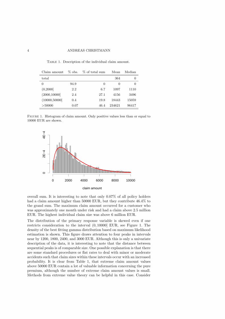
Figure 1. Histogram of claim amount. Only positive values less than or equal to10000 EUR are shown.

0 2000 4000 6000 8000 10000

02E

−4

4E−

4

claim amount

overall sum. It is interesting to note that only 0.07% of all policy holdershad a claim amount higher than 50000 EUR, but they contribute 46.4% tothe grand sum. The maximum claim amount occurred for a customer whowas approximately one month under risk and had a claim above 2.5 millionEUR. The highest individual claim size was above 6 million EUR.

The distribution of the primary response variable is skewed even if onerestricts consideration to the interval (0, 10000] EUR, see Figure 1. Thedensity of the best fitting gamma distribution based on maximum likelihoodestimation is shown. This figure draws attention to four peaks in intervalsnear by 1200, 1800, 2400, and 3000 EUR. Although this is only a univariatedescription of the data, it is interesting to note that the distance betweensequential peaks is of comparable size. One possible explanation is that thereare some standard procedures or flat rates to deal with minor or moderateaccidents such that claim sizes within these intervals occur with an increasedprobability. It is clear from Table 1, that extreme claim amount valuesabove 50000 EUR contain a lot of valuable information concerning the purepremium, although the number of extreme claim amount values is small.Methods from extreme value theory can be helpful in this case. Consider


Table 2. Maximum likelihood estimates for the parameters ξ and β of the Gen-eralized Pareto distributions used to model extreme claim amount values higherthan 50000 EUR. Confidence intervals at the 95% level are given in parenthesis.

data ξ 95% CI β 95% CI

all 0.804 (0.743, 0.865) 50035.42 (46813.48, 53257.37)

knot 1 0.887 (0.788, 0.985) 53357.66 (47959.25, 58756.08)

knot 2 0.635 (0.541, 0.728) 51214.80 (45919.53, 56510.07)

knot 3 0.852 (0.720, 0.984) 44742.58 (38588.19, 50896.97)

the Generalized Pareto distribution (GPD) with distribution function

Gξ,β =

{1− (1 + β−1ξx)−1/ξ if ξ 6= 01− exp(−x/β) if ξ = 0 ,

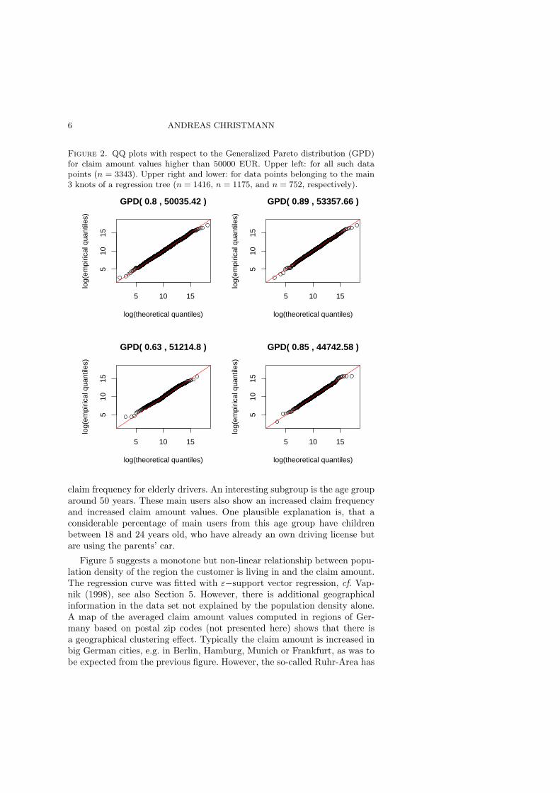
where x ≥ 0 if ξ ≥ 0, and x ∈ [0,−ξ−1] if ξ < 0, cf. Embrechts et al.(1997) and Celebrian et al. (2003). The parameter ξ is called the Paretoindex. The QQ plots given in Figure 2 show that the GPD can be usefulto fit extreme claim amount values. The upper left plot shows a QQ ploton logarithmic scales for all 3343 claim amount values higher than 50000EUR. The other three plots given in Figure 2 give the corresponding plotsfor claim amount values higher than 50000 EUR, which belong to the main3 knots of a regression tree constructed on the basis of a few importantexplanatory variables. The Pareto index for the data set of knot 2 differsfrom the Pareto indices from the other two knots, see Table 2. Note thathere we treat all extremes in a certain knot as realizations of independentand identically distributed random variables. Of course, one can fit morecomplex trees, but then the number of data points in the knots will decrease.We do not discuss such trees here, because the focus of this paper is noton the extreme values alone. Beirlant et al. (2002) proposed an alternativemethod to fit extreme claim amounts, see also Teugels (2003).

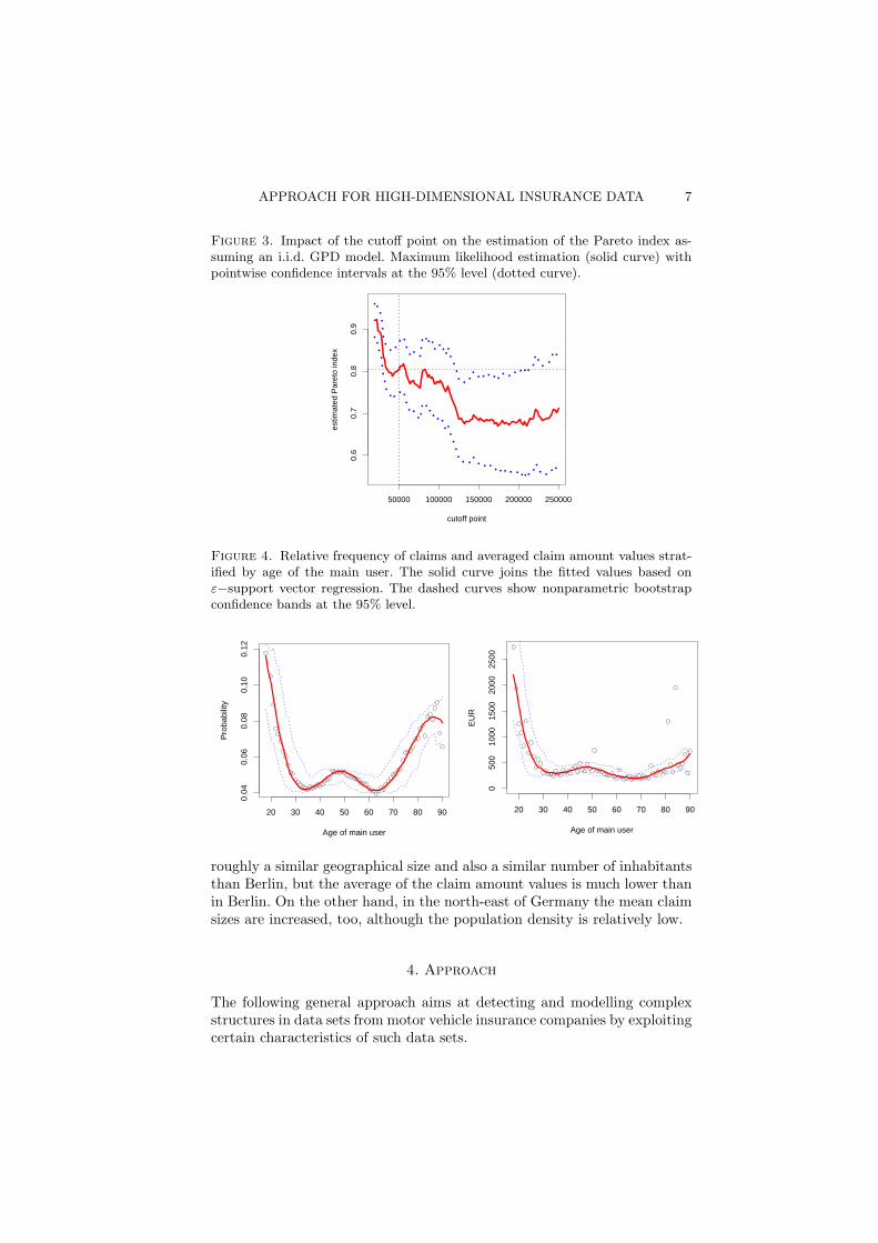
Figure 3 shows that the determination of the cutoff point can be crucialfor the estimate of the Pareto index. Here it was assumed for simplicity,that all extreme values above the specified cutoff point are realizations ofindependent and identically distributed random variables. The maximumlikelihood method was used to fit the GPD model. As before, such plotscan also be made for the main knots of a tree. The cutoff point of 50000EUR is used because it is similar to the cutoff point used by the Verbandoffentlicher Versicherer. We like to emphasize that the i.i.d. assumption isan oversimplification for the present data set.

Figure 4 shows the relative frequency that a claim occurred and theclaim amount stratified with respect to the age of the main user of the car.The smooth curve is the fit provided by ε−support vector regression, cf.Vapnik (1998). There is an interesting non-monotone relationship betweenthe age of the main user and both response variables. It is well-knownthat young drivers in Germany, say between 18 and 24 years old, have anincreased claim frequency. As was expected, the plot also shows an increased


Figure 2. QQ plots with respect to the Generalized Pareto distribution (GPD)for claim amount values higher than 50000 EUR. Upper left: for all such datapoints (n = 3343). Upper right and lower: for data points belonging to the main3 knots of a regression tree (n = 1416, n = 1175, and n = 752, respectively).

5 10 15

510

15

GPD( 0.8 , 50035.42 )

log(theoretical quantiles)

log(

empi

rical

qua

ntile

s)

5 10 15

510

15

GPD( 0.89 , 53357.66 )


log(

empi

rical

qua

ntile

s)

5 10 15

510

15

GPD( 0.63 , 51214.8 )


log(

empi

rical

qua

ntile

s)

5 10 15

510

15

GPD( 0.85 , 44742.58 )


log(

empi

rical

qua

ntile

s)

claim frequency for elderly drivers. An interesting subgroup is the age grouparound 50 years. These main users also show an increased claim frequencyand increased claim amount values. One plausible explanation is, that aconsiderable percentage of main users from this age group have childrenbetween 18 and 24 years old, who have already an own driving license butare using the parents’ car.

Figure 5 suggests a monotone but non-linear relationship between popu-lation density of the region the customer is living in and the claim amount.The regression curve was fitted with ε−support vector regression, cf. Vap-nik (1998), see also Section 5. However, there is additional geographicalinformation in the data set not explained by the population density alone.A map of the averaged claim amount values computed in regions of Ger-many based on postal zip codes (not presented here) shows that there isa geographical clustering effect. Typically the claim amount is increased inbig German cities, e.g. in Berlin, Hamburg, Munich or Frankfurt, as was tobe expected from the previous figure. However, the so-called Ruhr-Area has


Figure 3. Impact of the cutoff point on the estimation of the Pareto index as-suming an i.i.d. GPD model. Maximum likelihood estimation (solid curve) withpointwise confidence intervals at the 95% level (dotted curve).

50000 100000 150000 200000 250000

0.6

0.7

0.8

0.9

cutoff point

estim

ated

Par

eto

inde

x

Figure 4. Relative frequency of claims and averaged claim amount values strat-ified by age of the main user. The solid curve joins the fitted values based onε−support vector regression. The dashed curves show nonparametric bootstrapconfidence bands at the 95% level.

20 30 40 50 60 70 80 90

0.04

0.06

0.08

0.10

0.12

Age of main user

Pro

babi

lity

20 30 40 50 60 70 80 90

050

010

0015

0020

0025

00

Age of main user

EU

R

roughly a similar geographical size and also a similar number of inhabitantsthan Berlin, but the average of the claim amount values is much lower thanin Berlin. On the other hand, in the north-east of Germany the mean claimsizes are increased, too, although the population density is relatively low.

4. Approach

The following general approach aims at detecting and modelling complexstructures in data sets from motor vehicle insurance companies by exploitingcertain characteristics of such data sets.


Figure 5. Scatterplot of claim amount vs. population density.

0 5000 10000 15000

160

180

200

220

240

260

population density

clai

m a

mou

nt

1. Most of the policy holders have no claim within a year or a certain period.2. The claim sizes are extremely skewed to the right, but there is an atom

at zero.3. Extreme high claim amounts are rare events, but contribute enormously

to the total sum.4. There are only imprecise values available for some explanatory variables.5. Some claim sizes are only estimates.6. The data sets to be analyzed are huge.7. There is a complex, high-dimensional dependency structure between vari-

ables.Statistical procedures with good robustness properties are preferable dueto the features 3 to 5 in the list. Due to point 7 methods from statisticalmachine learning are of interest.

As before, let Yi denote the claim amount of customer i within a yearand xi the vector of explanatory variables. In the first step we construct anadditional stratification variable Ci by defining a small number of classesfor the values of Yi with a high amount of interpretability. For example,define a discrete random variable Ci with five possible values:

Ci =

0, if Yi = 0 ’no claim’1, if Yi ∈ (0, 2000] ’low claim amount’2, if Yi ∈ (2000, 10000] ’medium claim amount’3, if Yi ∈ (10000, 50000] ’high claim amount’4, if Yi > 50000 ’extreme claim amount’.

Of course, it depends on the application how many classes should be usedand how reasonable boundaries can be defined. We will not address thisproblem here. In the following the index i is sometimes omitted.

4.1. Approach A. Note that given the information that no claim occurred,it holds that

E(Y |C = 0, X = x) ≡ 0 . (1)


The law of total probability yields

E(Y |X = x) = P(C > 0|X = x)×∑k

c=1P(C = c|C > 0, X = x) · E(Y |C = c,X = x) , (2)

and we denote this formula as approach A. Note that in (2) the summa-tion starts with c = 1. Hence, it is only necessary to fit regression modelsto small subsets of the whole data set, see Table 1. However, one has toestimate the conditional probability P(C > 0|X = x) and the multi-classprobabilities P(C = c|C > 0, X = x) for c ∈ {1, . . . , k}, e.g. by a multi-nomial logistic regression model or by kernel logistic regression. If one splitsthe total data set into three subsets for training, validating, and testing,one only has to compute predictions for the conditional probabilities andthe corresponding conditional expectations for all data points. If the esti-mators of the conditional probabilities and the conditional expectations areconsistent, it follows by Slutzky’s theorem that the combination of these es-timators yields a consistent estimation of E(Y |X = x) in (2). Usually datasets in the context of motor vehicle insurance are huge, e.g. the data set inour application in Section 6 contains data from about 4.6 million customers.Bias reduction techniques applied to the validation data set may be helpfulto reduce a possible bias of the estimates.

From our point of view the indirect estimation of E(Y |X = x) via ap-proach A has practical and theoretical advantages over direct estimation ofthis quantity. Insurance companies are interested in estimating the termsin (2), because they contain additional information: the probability that acustomer has at least one claim (which is our secondary response variable),the conditional probabilities P(C = c|C > 0, X = x), and the conditionalexpectations E(Y |C = c,X = x). The approach circumvents the problem,that most observed claim amount values yi are 0, but P(Y = 0|X = x) = 0for many classical approaches based on a gamma or log-normal distribu-tion. A reduction of computation time is possible, because we only haveto fit regression models to a small subset (say 5%) of the data set. Theestimation of conditional class probabilities for the whole data set is oftenmuch faster than fitting a regression model for the whole data set. It ispossible, that different explanatory variables show a significant impact onthe response variable Y or on the conditional class probabilities for differ-ent classes defined by C. This can also result in a reduction of interactionterms. In principle, it is possible to use different variable selection methodsfor the k + 1 classes. This can be especially important for the class of ex-treme claim amount values: because there may be only some hundreds or afew thousands of these rare events in the data set, it is in general impossibleto use all explanatory variables for these data points. Finally, the strate-gies have the advantage that different techniques can be used for estimatingthe conditional class probabilities P(C = c|X = x) and for estimating theexpectations E(Y |C = c,X = x) for different values of C. Examples forreasonable pairs are:


• Multinomial logistic regression + Gamma regression• Robust logistic regression + semi-parametric regression• Multinomial logistic regression + ε-Support Vector Regression (ε-SVR)• Kernel logistic regression (KLR) + ε-Support Vector Regression• Classification trees + regression trees• A combination of the pairs given above, where some additional explana-

tory variables are constructed as a result of classification and regressiontrees or methods from extreme value theory are applied for the class ofextreme claim amount values.

For robust logistic regression see Kunsch et al. (1989) and Christmann(1994). Of course, ν−SVR (see Scholkopf and Smola, 2002) can be an in-teresting alternative to ε-SVR.

Even for data sets with several million of customers it is in general notpossible to fit simultaneously all high-dimensional interaction terms withclassical statistical methods such as logistic regression or gamma regression,because the number of interaction terms increases exponentially fast fornominal explanatory variables.

The combination of kernel logistic regression and ε−support vector re-gression (cf. Section 5), both with an RBF kernel has the advantage thatimportant interaction terms are fitted automatically without the need tospecify them manually.

We like to mention that some statistical software packages such as Rmay run into trouble in fitting multinomial logistic regression models forlarge and high-dimensional data sets. Three possible reasons are that thedimension of the parameter vector can be quite high, that a data set withmany discrete variables recoded into a large number of dummy variables willperhaps not fit into the memory of the computer, and that the maximumlikelihood estimate may not exist, cf. Christmann and Rousseeuw (2001).To avoid a multinomial logistic regression model one can consider all pairsand then use pairwise coupling, cf. Hastie and Tibshirani (1998).

4.2. Alternatives. The law of total probability offers alternatives to (2).The motivation for the following alternative, say approach B, is that we firstsplit the data into the groups ’no claim’ vs. ’claim’ and then split the datawith ’claim’ into ’extreme claim amount’ and the remaining k − 1 classes:

E(Y |X = x) = P(C > 0|X = x) × (3){P(C = k|C > 0, X = x) · E(Y |C = k,X = x) +

[1− P(C = k|C > 0, X = x)]×k−1∑c=1

P(C = c|0 < C < k,X = x) · E(Y |C = c, X = x)} .

This formula shares with (2) the property that it is only necessary to fitregression models to subsets of the whole data set. Of course, one can also


interchange the steps in the above formula, which results in approach C:

E(Y |X = x) = P(C = k|X = x) · E(Y |C = k,X = x) (4)+ [1− P(C = k|X = x)] · {P(C > 0|C 6= k, X = x)×

k−1∑c=1

P(C = c|0 < C < k, X = x) · E(Y |C = c,X = x)} .

Note that two big binary classification problems have to be solved in (4),whereas there is only one such problem in (3).

5. Kernel logistic regression and ε−support vector regression

In this section we briefly describe two modern methods based on convex riskminimization in the sense of Vapnik (1998), see also Scholkopf und Smola(2002).

In statistical machine learning the major goal is the estimation of a func-tional relationship yi ≈ f(xi) + b between an outcome yi belonging to someset Y ⊆ R and a vector of explanatory variables xi = (xi,1, . . . , xi,k)′ ∈ X ⊆Rp. The function f and the intercept parameter b are unknown. The esti-mate of (f, b) is used to get predictions of an unobserved outcome ynew basedon an observed value xnew. The classical assumption in machine learning isthat the training data (xi, yi) are independent and identically generatedfrom an underlying unknown distribution P for a pair of random variables(Xi, Yi), 1 ≤ i ≤ n. In applications the training data set is often quitelarge, high-dimensional and complex. The quality of the predictor f(xi)+ bis measured by some loss function L(yi, f(xi) + b). The goal is to find apredictor fP(xi) + bP which minimizes the expected loss, i.e.

EP L(Y, fP(X) + bP) = minf∈F , b∈R

EP L(Y, f(X) + b), (5)

where EP L(Y, f(X)+b) =∫

L(y, f(x)+b)dP(x, y) denotes the expectationof L with respect to P and F denotes an appropriate set of functions f :X → R. We have yi ∈ Y := {−1, +1} in the case of binary classificationproblems, yi ∈ Y := {0, 1, . . . , k} for multicategory classification problems,and yi ∈ Y ⊆ R in regression problems.

As P is unknown, it is in general not possible to solve the problem (5).Vapnik (1998) proposed to estimate the pair (f, b) as the solution of anempirical regularized risk. His approach relies on three important ideas:(1) restrict the class of functions f ∈ F to a broad subclass of functionsbelonging to a certain Hilbert space, (2) use a convex loss function L toavoid computational intractable problems which are NP-hard, and (3) usea regularizing term to avoid overfitting and to decrease the generalizationerror.


Let L : Y×R→ R be an appropriate convex loss function. Estimate (f, b)by solving the following empirical regularized risk minimization problem:

(fn,λ, bn,λ) = arg minf∈H, b∈R

1n

n∑

i=1

L(yi, f(xi) + b) + λ‖f‖2H, (6)

where λ > 0 is a small regularization parameter, H is a reproducing kernelHilbert space (RKHS) of a kernel k, and b is an unknown real-valued offset.The problem (6) can be interpreted as a stochastic approximation of theminimization of the theoretical regularized risk, i.e.:

(fP,λ, bP,λ) = arg minf∈H, b∈R

EP L(Y, f(X) + b) + λ‖f‖2H . (7)

In practice, it is often numerically better to solve the dual problem of (6). Inthis problem the RKHS does not occur explicitly, instead the correspondingkernel is involved. The choice of the kernel k enables the above methods toefficiently estimate not only linear, but also non-linear functions. Of specialimportance is the Gaussian radial basis function (RBF) kernel

k(x, x′) = exp(−γ‖x− x′‖2) , γ > 0, (8)

which is a universal kernel on every compact subset of Rd, cf. Steinwart(2001). Note, that γ in (8) describes the distance between two vectors x andx′. A radial basis function kernel offers not only a flexible fit but also a wayto spread the risk of a single customer to sub-populations of customers witha similar vector of explanatory variables. The tuning constant γ controlsthis similarity.

For the case of binary classification, popular loss functions depend on yand (f, b) via v = y(f(x) + b). Special cases are:

• Support Vector Machine (L1-SVM):L(y, f(x) + b) = max{1− y(f(x) + b), 0}

• Least Squares (L2-SVM):L(y, f(x) + b) = [1− y(f(x) + b)]2

• Kernel Logistic Regression (KLR):L(y, f(x) + b) = log(1 + exp[−y(f(x) + b)]), cf. Wahba (1999)

• AdaBoost:L(y, f(x)+b) = exp[−y(f(x)+b)], cf. Freund and Schapire (1996) andFriedman et al. (2000).

Kernel logistic regression has the advantage with respect to L1-SVM, thatit estimates log(P(Y =+1|X=x)

P(Y =−1|X=x) ), i.e. P(Y = +1|X = x) = (1 + e−[f(x)+b])−1,such that scoring is possible. Note that L1-SVM ’only’ estimates whetherP(Y = +1|X = x) is above or below 1

2 . Bartlett and Tewari (2004) show thatthere is a conflict in pattern recognition problems between the sparseness ofthe solution of kernel based convex risk minimization methods and the goalto estimate the conditional probabilities, see also Zhang (2004) for relatedwork. The sparseness of the L1-SVM solution is of course a consequence


of the fact that the L1-SVM uses a loss which is exactly equal to zero ify[f(x) + b)] > 1.

For the case of regression, Vapnik (1998) proposed the ε−support vectorregression (ε−SVR) which is based on the ε−insensitive loss function

Lε(y, f(x) + b) = max {0, |y − [f(x) + b]| − ε} ,

for some ε > 0. Note that only residuals y − [f(x) + b] lying outside of anε−tube are penalized. Strongly related to ε−support vector regression isν−support vector regression, cf. Scholkopf und Smola (2002).

Christmann and Steinwart (2004) showed that a large class of such con-vex risk minimization methods with a radial basis function kernel have goodrobustness properties, e.g. a bounded influence function and a bounded sen-sitivity curve.

6. Application

This section describes some results for applying the approach A, i.e. (2),to the data set from the Verband offentlicher Versicherer in Dusseldorf,Germany, see Section 3. We used a nonparametric approach based on thepair (KLR, ε−SVR) to fit the individual claim amount values per year. Thefollowing 8 explanatory variables were selected: gender of the main user,age of the main user, driving distance within a year, geographic region, avariable describing whether the car is kept in a garage, a variable for thepopulation density, a variable related to the number of years the customerhad no claim, and the strength of the engine.

We used a binary logistic regression model to fit the conditional proba-bilities that P(C > 0|X = x) (SAS, PROC LOGISTIC). The classical esti-mator in binary logistic regression is the maximum likelihood estimator. Ifthe data set has complete separation or quasi-complete separation, the max-imum likelihood estimates do not exist. Most statistical software packagesdo not check whether the maximum likelihood estimates exist. Christmannand Rousseeuw (2001) developed software to check whether the data set hascomplete or quasi-complete separation. Christmann et al. (2002) comparedsuch methods with methods based on Vapnik’s support vector machine witha linear kernel. Rousseeuw and Christmann (2003) proposed the hidden lo-gistic regression model, which is strongly related to logistic regression, andinvestigated estimates which always exist.

The conditional probabilities P(C = c|C > 0, X = x), 1 ≤ c ≤ 4, wereestimated via kernel logistic regression. First, we estimated the probabilitiesfor all pairs P(C = j|C ∈ {i, j}, X = x), where 1 ≤ i < j ≤ 4. Keerthi etal. (2002) developed a fast dual algorithm for kernel logistic regression forthe case of pattern recognition. Ruping (2003) implemented this algorithmin the program myKLR. We used myKLR to estimate the probabilitiesfor these pairs. Then the multi-class probabilities P(C = c|C > 0, X =x), c ∈ {1, 2, 3, 4}, were computed with pairwise coupling, cf. Hastie and


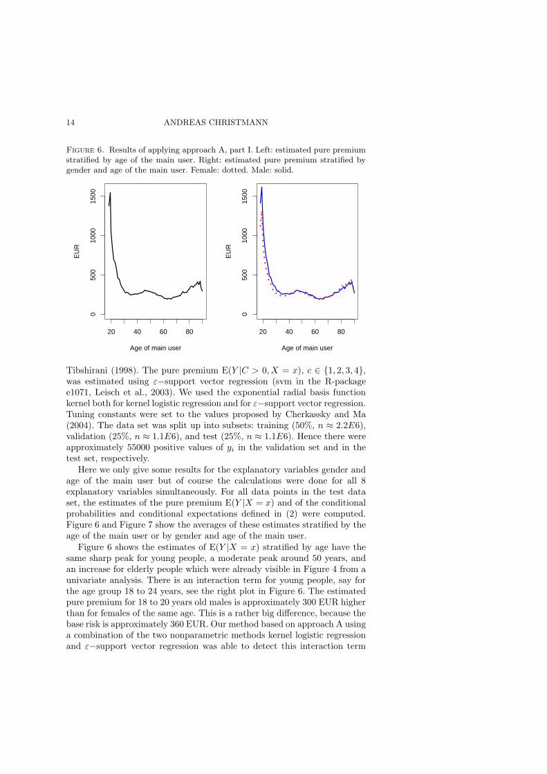
Figure 6. Results of applying approach A, part I. Left: estimated pure premiumstratified by age of the main user. Right: estimated pure premium stratified bygender and age of the main user. Female: dotted. Male: solid.

20 40 60 80

050

010

0015

00

Age of main user

EU

R

20 40 60 80

050

010

0015

00

Age of main user

EU

R

Tibshirani (1998). The pure premium E(Y |C > 0, X = x), c ∈ {1, 2, 3, 4},was estimated using ε−support vector regression (svm in the R-packagee1071, Leisch et al., 2003). We used the exponential radial basis functionkernel both for kernel logistic regression and for ε−support vector regression.Tuning constants were set to the values proposed by Cherkassky and Ma(2004). The data set was split up into subsets: training (50%, n ≈ 2.2E6),validation (25%, n ≈ 1.1E6), and test (25%, n ≈ 1.1E6). Hence there wereapproximately 55000 positive values of yi in the validation set and in thetest set, respectively.

Here we only give some results for the explanatory variables gender andage of the main user but of course the calculations were done for all 8explanatory variables simultaneously. For all data points in the test dataset, the estimates of the pure premium E(Y |X = x) and of the conditionalprobabilities and conditional expectations defined in (2) were computed.Figure 6 and Figure 7 show the averages of these estimates stratified by theage of the main user or by gender and age of the main user.

Figure 6 shows the estimates of E(Y |X = x) stratified by age have thesame sharp peak for young people, a moderate peak around 50 years, andan increase for elderly people which were already visible in Figure 4 from aunivariate analysis. There is an interaction term for young people, say forthe age group 18 to 24 years, see the right plot in Figure 6. The estimatedpure premium for 18 to 20 years old males is approximately 300 EUR higherthan for females of the same age. This is a rather big difference, because thebase risk is approximately 360 EUR. Our method based on approach A usinga combination of the two nonparametric methods kernel logistic regressionand ε−support vector regression was able to detect this interaction term


automatically although we did not model such an interaction term. It wasconfirmed by the Verband offentlicher Versicherer, that this interaction termis not an artefact, but typical for their data sets.

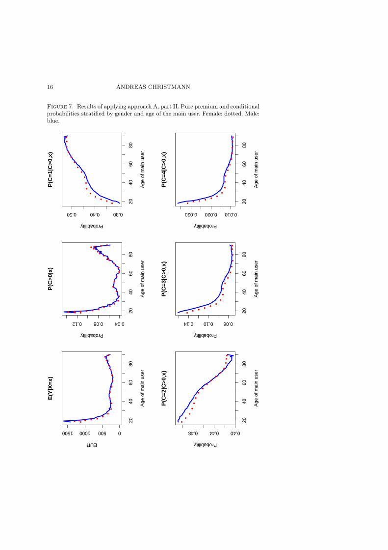
However, from our point of view the main strength of approach A be-comes visible if one investigates the conditional probabilities and conditionalexpectations which were fit by (2). Figure 7 shows the conditional proba-bilities stratified by gender and age of the main user. The probability ofa claim, i.e. P(C > 0|X = x), shows again a similar shape than the cor-responding curve in Figure 4. However, the conditional probability of aminor claim in the interval (0, 2000] EUR given the event that at least oneclaim occurred increases for people of at least 18 years, cf. the subplot forP(C = 1|C > 0, X = x) in Figure 7. This is in contrast to the correspondingsubplots for medium, high or extreme pure premium values, see the sub-plots for P(C = c|C > 0, X = x), c ∈ {2, 3, 4} in Figure 7. Especially thelast two subplots show, that young people have a two to three times higherprobability in producing a high claim amount than more elderly people.

The effect of gender and age of the main user on E(Y |C = c,X = x),c ∈ {1, . . . , 4}, was also investigated. The impact of these two explanatoryvariables on the conditional expectation of Y is lower than for the condi-tional probabilities, and the corresponding plots are omitted here. Neverthe-less, it was visible that young people have a higher estimated pure premiumthan more elderly people, even if one conditions with respect to the classvariable C.

Concluding, people belonging to the age group 18 to 24 years have ahigher estimated pure premium and a higher estimated probability to havea claim than more elderly customers. Approach A offers a lot of addi-tional information. The application of the pair kernel logistic regression andε−support vector regression was able to detect automatically an interactionterm for young people with respect to gender and a moderate increased purepremium for main users with an age around 50 years.

7. Discussion

In this paper certain characteristics of complex and high-dimensional datasets from motor vehicle insurance companies were described. We propose toestimate the pure premium in motor vehicle insurance data in an indirectmanner. This approach may also be useful in other areas, e.g. credit riskscoring, customer relationship management (CRM) or CHURN analyses.

There are several advantages of this approach in contrast to a straightfor-ward estimation of the pure premium. The approach exploits knowledge ofcertain characteristics of data sets from motor vehicle insurance companiesand estimates conditional probabilities and conditional expectations giventhe knowledge of an auxiliary class variable C describing the magnitude ofthe pure premium. This proposal offers additional insight into the structureof the data set, which is not visible with a direct estimation of the purepremium alone. Such additional information can be valuable for insurance


Figure 7. Results of applying approach A, part II. Pure premium and conditionalprobabilities stratified by gender and age of the main user. Female: dotted. Male:blue.

2040

6080

050010001500

E(Y

|X=x

)

Age

of m

ain

user

EUR

2040

6080

0.040.080.12

P(C

>0|x

)

Age

of m

ain

user

Probability

2040

6080

0.300.400.50

P(C

=1|C

>0,x

)

Age

of m

ain

user

Probability

2040

6080

0.400.440.48

P(C

=2|C

>0,x

)

Age

of m

ain

user

Probability

2040

6080

0.060.100.14

P(C

=3|C

>0,x

)

Age

of m

ain

user

Probability

2040

6080

0.0100.0200.030

P(C

=4|C

>0,x

)

Age

of m

ain

user

Probability


companies and can also be useful for aspects not related to the constructionof insurance tariffs, e.g. in the context of direct marketing. Further, differentestimation techniques and different variable selection methods can be usedfor the classes of pure premium defined by the auxiliary variable C.

The application of the proposed approach was illustrated for a large dataset containing data from 15 motor vehicle insurance companies from Ger-many. An explorative data analysis shows that there are complex and non-monotone dependency structures in this high-dimensional data. We used anonparametric approach based on a combination of kernel logistic regres-sion and ε−support vector regression. Both techniques belong to the classof statistical machine learning methods based on convex risk minimization,see Vapnik (1998), Scholkopf and Smola (2002), and Hastie et al. (2001).Such methods can fit quite complex data sets and have good predictionproperties. The combination of these methods was able to detect an inter-esting interaction term and violations of a monotonicity assumption withoutthe necessity that the researcher has to model interaction terms or polyno-mial terms manually. Although the combination of kernel based methodsfrom modern statistical machine learning yields some interesting insightsinto the insurance data set in our application, other pairs of methods toestimate the conditional probabilities and conditional expectations may bemore successful for other data sets.

Christmann and Steinwart (2004) showed that a large class of such con-vex risk minimization methods with a radial basis function kernel havebesides many other interesting properties also good robustness properties.Special cases are kernel logistic regression and the support vector machine(L1-SVM). Robustness is an important aspect in analyzing insurance datasets, because some explanatory variables may only be measured in an im-precise manner and some reported values of the claim size are only estimatesand not the true values. On the other hand, in contrast to some other areasof applied statistics, extreme high individual claim amount values per yearcan not be dropped from the data set because this would systematicallyunderestimate the pure premium.

In the literature it is often recommended to determine the tuning con-stants for kernel logistic regression and for ε−support vector regression, sayccost, λ, γ, and ε, via a grid search or by cross-validation. Such methodscan be extremely time-consuming for such a big data set we were deal-ing with in Section 6. Some preliminary experiments are indicating thatthese constants can be chosen in a reasonable way if they are determinedas the solution of an appropriate optimization problem, e.g. by minimizingthe mean squared error of the predictions for the validation data set or byusing a chi-squared type statistic similar to the one used by the Hosmer-Lemeshow test for checking goodness-of-fit in logistic regression models, c.f.Hosmer and Lemeshow (1989) or Agresti (1996). The Nelder-Mead algo-rithm, c.f. Nelder and Mead (1965), worked well in this context for sometest data sets and needed much less computation time than a grid search,but a systematic investigation of this topic is beyond the scope of this paper.


Although there were approximately 3300 customers with an individualclaim amount above 50000 EUR in the data set we used for illustrationpurposes, an attractive alternative to ε−support vector regression for thissubgroup is extreme value theory, e.g. by fitting generalized Pareto distri-butions of the main knots of a tree or more sophisticated methods.

Now, a brief comparison of the approach described in this paper andwell-known methods for constructing insurance tariffs is given. The gen-eral approach described in this paper can be used to complement – not toreplace – traditional methods which are used in practice to construct in-surance tariffs, see e.g. Bailey and Simon (1960) or Mack (1997). The goalof our approach is to extract additional information which may be hardto detect or to model by classical methods. Generalized linear models be-long to the most successful methods to construct insurance tariffs, see e.g.McCullagh and Nelder (1989), Kruse (1997), and Walter (1998). General-ized linear models are flexible enough to construct regression models forresponse variables with a distribution from an exponential family, e.g. Pois-son, Gamma, Gaussian, inverse Gaussian, binomial, multinomial or negativebinomial distribution. However, the assumptions of generalized linear mod-els are not always satisfied. Generalized linear models are still parametricmodels and the classical maximum likelihood estimator in such models is ingeneral not robust, see e.g. Christmann (1994, 1998), Cantoni and Ronchetti(2001), and Rousseeuw and Christmann (2003). Further, generalized linearmodels assume a certain functional relationship between expectation andvariance even if one allows that over-dispersion is present. Tweedie’s com-pound Poisson model, see Smyth and Jørgensen (2002), is even more flexiblethan the generalized linear model because it contains not only a regressionmodel for the expectation of the response variable Y but also a regressionmodel for the dispersion of Y . However, this more general model still yieldsproblems in modelling complex high-dimensional relationships, especially ifmany explanatory variables are discrete which is quite common for insur-ance data sets. E.g., if there are 8 discrete explanatory variables each with 8different values there are approximately 88 ≈ 16.7 million interaction termspossible. Usually a data set from a single motor vehicle insurance companyin Germany has much less observations. One can circumvent some of thedrawbacks which generalized linear models or Tweedie’s compound Pois-son model have by using nonparametric methods from modern statisticalmachine learning theory such as support vector regression or kernel logisticregression. A radial basis function kernel offers not only a flexible nonpara-metric fit but also a way to spread the risk of a single customer to sub-populations of customers with a similar vector of explanatory variables byspecifying the constant γ in an appropriate manner. But even if the analystchooses classical methods such as logistic regression and gamma regressionto estimate the conditional probabilities and the conditional expectations in(2), the approach described in this paper may yield additional insight intothe structure of the data set, because one can investigate whether these


conditional probabilities and conditional expectations differ with respect tosubgroups defined by the class variable C.

Bibliography

Agresti, A. (1996). An Introduction to Categorical Data Analysis. Wiley, NewYork.

Bailey, R. A., Simon, L.J. (1960). Two studies in automobile insurance ratemak-ing. ASTIN Bulletin 1 192–217.

Bartlett, P. L., Tewari, A. (2004). Sparseness vs Estimating ConditionalProbabilities: Some Asymptotic Results. Preprint, University of California,Berkeley.

Beirlant, J., de Wet, T., Goegebeur, Y. (2002). Nonparametric Estimationof Extreme Conditional Quantiles. Technical Report 2002-07, Universitair Cen-trum voor Statistiek, Katholieke Universiteit Leuven.

Cantoni, E., Ronchetti, E. (2001). Robust Inference for Generalized LinearModels. Journal of the American Statistical Association 96 1022–1030.

Celebrian, A.C., Denuit, M., Lambert, P. (2003). Generalized Pareto Fit tothe Society of Actuaries’ Large Claims Database. North American ActuarialJournal 7 18–36.

Cherkassky, V., Ma, Y. (2004). Practical selection of SVM parameters andnoise estimation for SVM regression. Neural Networks 17 113–126.

Christmann, A. (1994). Least median of weighted squares in logistic regressionwith large strata. Biometrika 81 413–417.

Christmann, A. (1998). On positive breakdown point estimators in regressionmodels with discrete response variables. Habilitation thesis, University of Dort-mund, Department of Statistics.

Christmann, A., Fischer, P., Joachims, T. (2002). Comparison between vari-ous regression depth methods and the support vector machine to approximatethe minimum number of misclassifications. Computational Statistics 17 273–287.

Christmann, A., Rousseeuw, P.J. (2001). Measuring overlap in logistic regres-sion. Computational Statistics and Data Analysis 37 65–75.

Christmann, A., Steinwart, I. (2004). On robust properties of convex riskminimization methods for pattern recognition. Journal of Machine LearningResearch 5 1007-1034.

Embrechts, P., Kluppelberg, C., Mikosch, T. (1997). Modelling ExtremeEvents for Insurance and Finance. Springer, Berlin.

Freund, Y., Schapire, R. (1996). Experiments with a new boosting algorithm.In Machine Learning: Proceedings of the 13th International Conference. (L.Saitta, ed.), 148–156. Morgan Kaufmann, San Francisco.

Friedman, J., Hastie, T., Tibshirani, R. (2000). Additive logistic regression: astatistical view of boosting (with discussion). Annals of Statistics 28 337–407.

Hastie, T., Tibshirani, R. (1998). Classification by pairwise coupling. Annalsof Statistics 26 451–471.


Hastie, T., Tibshirani, R., Friedman, J. (2001). The Elements of StatisticalLearning. Data Mining, Inference and Prediction. Springer, New York.

Hosmer, D.W., Lemeshow, W. (1989). Applied Logistic Regression. Wiley, NewYork.

Keerthi, S.S., Duan, K., Shevade, S.K., Poo, A.N. (2002). A fast dual algo-rithm for kernel logistic regression. Preprint, National University of Singapore.

Kruse, O. (1997). Modelle zur Analyse und Prognose des Schadenbedarfs in derKraftfahrt-Haftpflichtversicherung. Verlag Versicherungswirtschaft e.V., Karls-ruhe.

Kunsch, H.R., Stefanski, L.A., Carroll, R.J. (1989). Conditionally Unbi-ased Bounded-Influence Estimation in General Regression Models, With Ap-plications to Generalized Linear Models. Journal of the American StatisticalAssociation 84 460–466.

Leisch, F. et al. (2003). R package e1071. http://cran.r-project.org.

Mack, T. (1997). Versicherungsmathematik. Verlag Versicherungswirtschaft e.V.,Karlsruhe.

McCullagh, P., Nelder, J.A. (1989). Generalized linear models, 2nd ed.. Chap-man & Hall, London.

Nelder, J. A., Mead, R. (1965). A simplex algorithm for function minimization.Computer Journal 7 308–313.

R Development Core Team (2004). R: A language and environment for sta-tistical computing. R Foundation for Statistical Computing, R Foundation forStatistical Computing.

Rousseeuw, P.J., Christmann, A. (2003). Robustness against separation andoutliers in logistic regression. Computational Statistics & Data Analysis 43315–332.

Ruping, S. (2003). myKLR - kernel logistic regression. Department of ComputerScience, University of Dortmund,http://www-ai.cs.uni-dortmund.de/SOFTWARE.

SAS Institute Inc. (2000). SAS/STAT User’s Guide, Version 8. Cary, NC: SASInstitute Inc..

Scholkopf, B., Smola, A. (2002). Learning with Kernels. Support Vector Ma-chines, Regularization, Optimization, and Beyond. MIT Press, Cambridge.

Smyth, G. K., Jørgensen, B. (2002). Fitting Tweedie’s compound Poissonmodel to insurance claims data: dispersion modelling. ASTIN Bulletin 32143–157.

Steinwart, I. (2001). On the Influence of the Kernel on the Consistency of Sup-port Vector Machines. Journal of Machine Learning Research 2 67–93.

Teugels, J.L. (2003). Reinsurance Actuarial Aspects. EURANDOM, Report2003-006.

Vapnik, V. (1998). Statistical Learning Theory. Wiley, New York.

Wahba, G. (1999). Support Vector Machines, Reproducing Kernel Hilbert Spacesand the Randomized GACV. In Advances in Kernel Methods - Support VectorLearning (B. Scholkopf, C.J.C. Burges, A.J. Smola, eds.), 69–88. MIT Press,Cambridge, MA.


Walter, J.T. (1998). Zur Anwendung von Verallgemeinerten Linearen Modellenzu Zwecken der Tarifierung in der Kraftfahrzeug-Haftpflichtversicherung. Ver-lag Versicherungswirtschaft e.V., Karlsruhe.

Zhang, T. (2004). Statistical behavior and consistency of classification methodsbased on convex risk minimization. Annals of Statistics 32 56-134.

Andreas ChristmannUniversity of DortmundDepartment of Statistics44221 [email protected]

An approach to model complex high-dimensional insurance data · 2019-09-21 · An approach to model...

Documents

Transcript of An approach to model complex high-dimensional insurance data · 2019-09-21 · An approach to model...