1

An Approach to Model and Predict the Popularityof Online Contents with Explanatory Factors

Jong Gun Lee∗, Sue Moon† and Kave Salamatian‡∗UPMC-Paris Universitas, †KAIST and ‡Universite de Savoie

∗jonggun.lee@lip6.fr, †sbmoon@kaist.edu and ‡kave.salamatian@univ-savoie.fr

Abstract—In this paper, we propose a methodology to predictthe popularity of online contents. More precisely, rather thantrying to infer the popularity of a content itself, we infer thelikelihood that a content will be popular. Our approach is rootedin survival analysis where predicting the precise lifetime of anindividual is very hard and almost impossible but predicting thelikelihood of one’s survival longer than a threshold or anotherindividual is possible. We position ourselves in the standpoint ofan external observer who has to infer the popularity of a contentonly using publicly observable metrics, such as the lifetime ofa thread, the number of comments, and the number of views.Our goal is to infer these observable metrics, using a set ofexplanatory factors, such as the number of comments and thenumber of links in the first hours after the content publication,which are observable by the external observer.

We use a Cox proportional hazard regression model that di-vides the distribution function of the observable popularity metricinto two components: a) one that can be explained by the givenset of explanatory factors (called risk factors) and b) a baselinedistribution function that integrates all the factors not takeninto account. To validate our proposed approach, we use datasets from two different online discussion forums: dpreview.com,one of the largest online discussion groups providing newsand discussion forums about all kinds of digital cameras, andmyspace.com, one of the representative online social networkingservices. On these two data sets we model two different popularitymetrics, the lifetime of threads and the number of comments, andshow that our approach can predict the lifetime of threads fromDpreview (Myspace) by observing a thread during the first 5∼6days (24 hours, respectively) and the number of comments ofDpreview threads by observing a thread during first 2∼3 days.

I. INTRODUCTION

The emergence of Web 2.0 and online social networkingservices, such as Digg, YouTube, Facebook, and Twitter, haschanged how users generate and consume online contents.As the YouTube report of 20 hours worth of video uploadevery minute demonstrates1, the amount of user-generatedcontents is growing fast. Via online social networking servicesaugmented with multimedia contents support, sharing andcommenting on other users’ contents constitute a significantpart of today’s Internet users’ web experience. Then howdo users find contents that are interesting? How do certaincontents rise in popularity? If we can predict such rise, we canpick those mostly likely to get popular and filter out others.Such a mechanism will be extremely expedient to users in thisage of information deluge.

The popularity of an online content is not a well-defined,but highly subjective term, which can be defined as a mixture

1http://www.youtube.com/t/fact sheet (accessed on Mar 26, 2010)

of endogenous and exogenous factors. The choice of factorsvaries from a person to another and from a content to another.Also, we note that accessibility and observability of the datathat represent those factors may not be universal. Thus inorder to model the popularity of online contents, we first haveto decide how we define “popularity”. What factors do wetake into consideration and which explicit data and relatedmeasures shall we use to represent popularity?

Here we take the standpoint of an individual user who hasto infer the popularity of a content from publicly observabledata, such as the lifetime of threads and the number ofcomments. Individual users have differing views of popularityand measures of choice will be different. Our goal is to developa general framework that could accommodate differing viewsby allowing users to choose contributing factors.

Multiple factors, however, complicate the accurate predic-tion of online contents popularity. The popularity of contentsis sometime unpredictable by nature. For example, the flurryof contents and reactions happening very early, even beforeconfirmation, of the death of Michael Jackson was probably farmore than what could have been predicted by any model. Somecontents become increasingly popular over time demonstratinga cascading effect [1], and it is hard to predict what typeof contents will eventually instigate such a cascading effect.Last but not least, popularity relates in a complex way to thesocial psychology of the population of online content usersand capturing this intricate relation in a predictive model isdifficult. All these difficulties compound the effectiveness ofa predictive model.

Szabo and Huberman use a linear regression to predictthe long time popularity of an online content from earlymeasurement of user access pattern, based on an observationwhere the logarithmically transformed popularity of long timepopularity of a content is highly correlated with its earlymeasured popularity [2]. For an all-time popular content, theirapproach, however, produces large error because their purposeis to predict the exact value of its popularity. Our approach inthis paper differs from [2] and is rooted in survival analysis.It is used when predicting the precise lifetime of an individualis very hard. A patient with a cancerous metastasis mightstay alive much longer than predicted by its doctors, when ahealthy young person might die in a car accident. Nevertheless,predicting the likelihood where one will survive longer thana threshold or another individual is possible. In particular onecan evaluate the effect of risk factors; smoking is a risk factorthat makes a smoker less likely to be alive in a long term

2

compared to a non-smoking person. As in survival analysis,we do not aim at knowing the precise popularity of a contentbut our goal is to infer the likelihood (the probability) that acontent with given characteristics will attract popularity abovea given threshold.

We use a Cox proportional hazard regression model [3]. Itdivides the distribution function of the observable popularitymeasure into two components: (a) one that can be explained bythe given set of explanatory factors (called risk factors) and (b)a baseline distribution function that integrates all the factorsnot taken into account. This approach is frequently applied inbiostatistics to model human survival and in reliability theory.The Cox proportional hazard regression model is suitable toour purpose, because the regression does not assume anyparametric structure for the baseline hazard, which contains allfactors not taken into account. In fact the regression “integratesout”, or heuristically removes from consideration, the baselinehazard and maximizes the remaining partial likelihood. TheCox proportional model, therefore, separates the effects of theexplanatory parameter from the effects of all other possiblefactors in the baseline hazard distribution.

We validate our approach over datasets crawled from twoonline thread-based discussion forums: dpreview.com and mys-pace.com. Our data sets contain information about 267,000threads and 2.5 million comments. Defining the popularity ofa thread is difficult as these two forums do not provide anyinformation about the statistics about the contents. We assumethat the number of comments in a thread and the lifetime ofthe thread capture the popularity of a thread.

The contributions of our paper are:1) This work relates the popularity of an online content to

explanatory factors (risk factors). We show that survivalanalysis is applicable to predict the popularity of anonline content.

2) We implement the Cox proportional hazard regressionmodel with explanatory variables as risk factors to modeland predict a popularity metric.

3) We validate our approach by modeling two kinds of pop-ularity metrics, the lifetime of threads and the number ofcomments, with two different online discussion forumsand show that our proposed approach is able to predictthe likelihood of the fate of an online content after onlya short period of observation.

The remainder of this paper is structured as follows. InSection II we explain survival analysis and the Cox propor-tional hazard regression model and in Section III we describeour prediction methodology. Section IV gives our experimentresults of predicting the lifetime of threads and the numberof comments of threads. Finally we conclude this paper inSection VI.

II. BACKGROUND

In this section we give a brief introduction to survivalanalysis and the Cox proportional hazard regression model.

A. Survival AnalysisSurvival analysis is a branch of statistics that deals with

survival time until an event of failure or death. It is widely used

in biostatistics and reliability study. Throughout this paper, Trepresents a random variable denoting the time to a death eventand t the wall clock time, respectively. Survival analysis dealswith three main functions.

The failure function F (t) is the probability to fail beforea certain time t, i.e., the Cumulative Distribution Function(CDF) of the random variable T , F (t) = Pr {T ≤ t}. Thisdefinition can be extended to F (k) where k is a discreteincreasing variable, such as the number comments on a thread.

The survival function S(t) is the Complementary Cumula-tive Distribution Function (CCDF) of T , i.e., the dual of F (t),S(t) = 1−F (t) = Pr {T > t}. It is the probability of survivalup to a certain time t.

The hazard function h(t) gives the failure rate at time tconditioned on the instance being still alive at time t, i.e., theexpected number of failures happening at or close to time t,

h(t) =f(t)S(t)

= −S′(t)S(t)

(1)

One can define the cumulative hazard, denoted as H(t) asthe overall number of failures that are expected to happen upto time t. The cumulative hazard is related to the survivalfunction through the below relation:

H(t) =∫ t

0

h(u) du = −logS(t) (2)

For the discrete case, h(t) is replaced by h(k) defined as :

h(k) =f(k)S(k)

=(

1− S(k − 1)S(k)

)(3)

B. Cox Proportional Hazard Regression Model

Cox proportional hazard regression [3] is a semi-parametricapproach widely used in practice. In the forthcoming, wedescribe it given that the failure time is continuous. However,the analysis can be extended in a straightforward way to thecase where failure time is a discrete variable k.

The Cox proportional hazard regression fits a regressionmodel defined as a parametric linear function of a set of riskfactors to an empirical failure function; it assumes that thehazard function can represented as

h(t) = h0(t)× exp(β1x1 + β2x2 + · · ·+ βkxk). (4)

The hazard contains two components: a parametric part thatdepends linearly on the risk factors and a non-parametricpart defined as baseline hazard h0(t). In other terms, hazardfunction h(t) is decomposed into two components:

1) The risk factors {x1, ..., xk} that are the set of factorsthat influence the survival duration. As the risk factorsare introduced into an exponential function, their effectsbecome proportional, i.e., adding to the risk factor has amultiplicative effect on hazard function. Therefore, thecoefficients βi represents the relative importance of riskfactors.

2) The baseline hazard h0(t) that gives the natural risk,i.e., the hazard when any risk factor is not present. Noassumptions is made about the form of h0(t). Usingrelations between the cumulative hazard function and the

3

the survival function, one can define a baseline survivalfunction as S0(t) = exp(−

∫ t0h0(t)dt).

C. Interpretation of fitting results

We explain the interpretation of a risk factor in Cox propor-tional hazard regression with the following example shown inFigure 1. In the example, let’s S(t), presented by the dotted

0 10 20 30 40 50 60 70 80 90 1000

0.1

0.2

0.3

0.4

0.5

0.6

0.7

0.8

0.9

1

Time t

Surv

ival

Fun

ctio

n −

S(t)

SC(t)SB(t)

SA(t)

S(t)

S(t)SC(t)SB(t)SA(t)

Fig. 1. Examples for understanding risk factors(RFs) and survival function

line, the initial lifetime distribution observed empirically andSX(t) being the remaining baseline survival function afterfitting a Cox model with an unique risk factor X = {A,B,C}.In order words, SX(t) is the baseline hazard for the riskfactor X , i.e., the survival distribution if the risk factor Xis not present, and S(t) is the survival distribution when therisk factor X is present. The wider is the distance betweenS(t) and SX(t), the more effective is the risk factor X . Tosimplify the discussion in this example, we present a survivalfunction as a straight line. Figure 1 implies the followings:Due to the effect of the risk factor A, the overall lifetime isincreased. Depending on risk factors, the overall lifetime canbe increased, SA(t), or decreased, SB(t). Comparatively, riskfactor A is more significant risk factor rather than the riskfactor C.

III. PROPOSED METHODOLOGY

Formally we model the hazard function h(t) of an observ-able popularity metric, through a Cox proportional hazard re-gression, described in Section II. In this context, the popularitymetric can be any measure of the popularity of online contents(e.g., the thread lifetime or the number of received commentsof a thread in a discussion forum) and the risk factor are chosento impact the popularity (e.g., the number of comments, thenumber of contributors, and so on.)

A. Selecting a set of significant risk factors

Similarly to [2], we use as explanatory (risk) factors, earlyvalues of the content attributes that are visible to an externaluser, such as the initial number of comments and the initialnumber of view.

First of all, one should avoid to use highly correlated factorsas they are redundant and can reduce the quality of the fitting.So the first step for selecting the set of significant risk factorsis to check the correlation among the potential risk factors inorder to rule out the simultaneous usage of highly correlated(the ones with correlation higher than 0.8) factors.

After checking that the risk factors are not highly correlated,we can follow the approach explained in Section II-C to rankdifferent combination risk factors by comparing the baselinesurvival obtained after fitting the Cox regression model. Thefurther is the resulting baseline survival function from theempirical lifetime distribution, the more significant is this riskfactor.

B. Fitting the Cox proportional regression

After setting the set of risk factor to be studied, one canapply the Cox proportional regression to it and try to fitthe long-term empirical final distribution of popularities thatis obtained after the last activity (comment or view) of acontent. However we will fit different regression that aregenerated using different values of initial observation period.The aim of this step is to find an observation time when theinformation from risk factors are enough to obtain a goodprediction of the likelihoods of popular contents. The qualityof the prediction model is assessed by observing the resultingbaseline hazard; the further the baseline hazard goes from theempirical distribution the better becomes the predictive powerof the variables relative to this observation period.

C. Finding a baseline hazard function for the risk factors

Up to now, we did not provide any functional form forthe baseline survival function. The Cox Proportional Hazardregression gives a non parametric description of the baselinesurvival function that can be thereafter fitted to a parametricdistribution. Frequently a Weibull distribution [4] is used. TheWeibull distribution is characterized by two parameters: a scaleparameter λ and a shape parameter γ:

f(x : λ, γ) =γ

λ(x

λ)(γ−1)

e−( xλ )γ (5)

The CDF of a Weibull distribution is given by Equation 6.

Pr(T > t) = 1− e−( tλ )γ (6)

From Equation (7), we can present a baseline cumulativehazard function like Equation (8).

S0(t) = e−( tλ )γ (7)

H0(t) = (t

λ)γ (8)

So h0(t) can be approximated by h0(t) = γλ

(tλ

)γ−1.

D. Forecasting the lifetime likelihood

Having the fitted values of the Cox regression parameters(the βi obtained in second step) and the parameter of Weibulldistribution obtained above, one can retrieve an approximationof the total hazard function through

h(t) =γ

λ

(t

λ

)γ−1

exp(β1x1 + β2x2 + · · ·+ βkxk)

and using Eq. 2 retrieves an approximation of the empiricalsurvival distribution.

4

IV. EXPERIMENT

In this section, we describe our datasets (Section IV-A)and present the experiment result on modeling two differentpopularity metrics, the lifetime of threads (Section IV-B) andthe number of comments per thread (Section IV-C).

A. Datasets

We made two datasets, D-dpreview and D-myspace, fromonline discussion forum services of forums.dpreview.com andforum.myspace.com and we present the brief description ofthe datasets in Table I. Dataset D-dpreview contains the

Dataset Service Topic Start - End

D-dpreview forum.dpreview.com Canon 40D-10D 2003/01 ∼ 2007/12D-myspace forums.myspace.com Music - General 2004/01 ∼ 2008/04

dataset # threads (T) # comments (C) Uall UT UC

D-dpreview 140,524 1,496,808 44,955 27,989 41,269D-myspace 127,607 1,038,989 - - -Uall: the number of unique postersUT : the num. of unique thread posters, UC : the num. of unique comment posters

TABLE IDESCRIPTION OF DATA SETS FOR EXPERIMENT

information of the entire threads and comments of CanonEOS 40D-10D discussion forum for 5 years from 2003 to2007. We made D-myspace by crawling all of threads andcomments of Music-General forum from the creation of theforum to May 2008. For each post, a thread or a comment, wecollected its posted timestamp and when making D-dpreviewwe additionally crawled the anonymized poster identifier foreach post2. Overall two datasets have more than 267,000threads and 2.5 millions of comments and in D-dpreview thereare about 45,000 unique posters.

Before applying our approach to model the lifetime ofthreads and the number of comments of threads, we need todefine the lifetime of a thread. It can be defined in many ways.We will use the following definition: the lifetime of a thread isthe time difference between the posting time of the thread andthe posting time of its last comment. However it is not possibleto decide if a comment is the definitive last comment. We havetherefore to define the lifetime of a thread by assuming thata thread being dead if it does not receive any new commentduring a thread expiration time. To decide the expiration timewe use inter-comments time and set this value to five days(resp. two days ) for D-dpreview (resp. D-myspace) as only0.5% of comments arrive later3.

B. Modeling the Lifetime of Threads

In order to model the lifetime of threads of discussion fo-rums, we use the information from user comments as explana-tory factors because as an external observer, we can access tothese information. From the information, we extract two kindsof information, a) overall user interests on a discussion threadand b) temporal user interests on it. About the overall user

2We could not collect any poster identifier for D-myspace because theinformation was hidden.

3Indeed other expiration time can be used such as 99% or 99.9%.

interests on a thread, we assume that a user leaves commentson a thread that is interesting to her. Based on this assumption,we consider the following three potential explanatory factors.The last two factors are used to separate the effects of authorherself from others.

1. the overall number of comments of a thread2. the number of comments by author of its original post3. the number of unique posters except author of theoriginal one

About temporal user interests, we used the inter-commentingtimes. To receive a high rate of comments for a thread can bea sign when the content is interesting. Thus we consider thefollowing four information as potential factors.

4. the time until the first comment5. the median of inter-comments time6. the mean of inter-comments time7. the variance of inter-comments time

Among the above seven potential explanatory factors, werule out useless factor which do not capture For this, in Figure2 we plot the empirical survival function of D-dpreview andseven baseline survival functions with seven factors. The line

0 1 2 3 4x 106

10−4

10−3

10−2

10−1

100

time (second)

Surv

ival

Fun

ctio

n S(

t)

Empirical CCDF1. Num. comments2. Time until first comm.3. Num. comm. by author4. Num. contributors5. Median of intercomm.6. Mean of intercomm.7. Variance of intercomm.

271

3

64 5

Fig. 2. Selecting significant risk factors (D-dpreview)

named as Empirical CCDF shows the survival function, i.e., theCCDF of the empirical lifetime distribution, obtained over D-dpreview and each curve tagged by a number between 1 and 7is the baseline survival function when the explanatory factor ofthe tagged number is used as a risk factor for a Cox regressionmodel. This figure shows that out of seven, two distributionstagged by 2 and 5 are almost same as Empirical CCDF. So wedo not use these factors as risk factors and in the followingwe consider the five potential explanatory factors as below.

1. the number of comments,3. the number of comments by a thread poster,4. the number of comment contributors,6. the mean of inter-comment time,7. the variance of inter-comment time.

In order to excluding redundant factors among the fivefactors, we use correlation coefficient. Correlation coefficientR(x, y) between two variables, x and y, is defined as:

R(x, y) =covariance(x, y)√

variance(x)× variance(y), (9)

where |R(x, y)| ∼ 1 means that they are highly correlated but|R(x, y)| ∼ 1 implies that they are lowly correlated.

Table II shows the correlation coefficient between twofactors and it implies that the first explanatory factor is highly

5

RF 1 3 4 6 71 1.0000 0.6429 0.9124 -0.0004 0.10003 0.6429 1.0000 0.4777 0.1000 0.10004 0.9124 0.4777 1.0000 0.0000 0.10006 -0.0004 0.1000 0.0000 1.0000 0.85307 0.1000 0.1000 0.1000 0.8530 1.0000

TABLE IICORRELATION COEFFICIENT BETWEEN TWO RISK FACTORS (RFS).

EACH NUMBER FOR RF IS THE SAME ONE USED IN FIGURE 2

correlated to the fourth one. Thus, instead of using bothfactors, we use only the first one because it captures muchmore information than the fourth one as illustrated in Figure2. Now with four explanatory factors, named with 1, 3, 6, and7, we make all possible combinations of the factors and thenpresent baseline survival distributions when each combinationof factors is used as risk factors in Figure 3. Since based

0 5 10 15 20 25 30 35 40

10−4

10−3

10−2

10−1

100

Thread lifetime (day)

Base

line

surv

ival

func

tion

for g

iven

risk

fact

or(s

)

1, 3, 6, 71, 3, 61, 3, 73, 6, 71, 31, 61, 73, 63, 76, 71367

1.6 1.8 2 2.2 2.4 2.6 2.8 310−4

10−3

10−2

1, 3, 6, 7

1, 3, 7

1, 71, 3, 6

1, 6

Fig. 3. Ranking the different combinations of risk factorsThe rightest line shows the empirical thread lifetime.

on the figure to use all four factors makes the best baselinesurvival function among them, we use the four factors in ourmodeling. For D-myspace, we use three factors by excluding3. the number of comments by a thread poster because we donot have user identifier information in D-myspace.

In Figure 4(a) and 4(d), we plot S(t) and S0(t) when weintroduce the risk factors to Cox proportional hazard modelswith D-dpreview and D-myspace, respectively. In order topresent S0(t) as a functional form, we fit a Weibull distri-bution for each baseline hazard function and we present thefitted Weibull distribution for each baseline failure function,1 − S0(t), in Figure 4(b) and 4(e). From these fittings wecan represent a cumulative baseline hazard function with scaleand shape parameters of the Weibull distribution and finallywe find that H0(t) are ( t

0.4286 )0.9909 for D-dpreview and( t0.101 )0.8616 for D-myspace.In Figure 4(c) and Figure 4(f) we show the process to find

the minimum observation time for D-dpreview and D-myspace.In each figure, we plot the empirical lifetime distribution(empirical CCDF), the baseline survival function capturedduring the whole thread duration, and a set of baseline survivalfunctions captured a certain observation time. Remind thatthe gap between an empirical CCDF and a baseline survivalfunction during the whole thread duration is the informationbased on the whole thread lifetime. Thus the aim of this stepis to find a certain time point where the information capturedfrom the time is close to the information captured from thewhole lifetime. For instance, in Figure 4(c) ‘BSF after 1

day’ shows the baseline survival function when user commentinformation captured during the first day is introduced to riskfactors of a Cox proportional hazard model. The curve of ‘BSFafter 1 day’ is too close to the curve of ‘empirical CCDF’. Itmeans that the information captured during the first one dayis not enough to predict the lifetime of threads of D-dpreview.Thus based on these figures, we say that we are able to closelypredict the empirical lifetime of D-dpreivew and D-myspace byobserving the first five to six days and 24 hours, respectively.

By the nature of survival analysis, long-lived instanceslikely have less hazard than short-lived instances. To seeour models follows this fact, we plot risk factor component(β1x1 + β2x2 + ...+ βkxk) against the lifetime of threads inFigure 5. Based on this figure we verify that our two modelsfor two datasets produce relatively less hazard values for long-lived threads and relatively much hazard values for short-livedthreads4.

(a) D-dpreview (b) D-myspace

Fig. 5. risk factor component (x1β1...xkβk) vs. the lifetime of threads

To see the relation between an observation time and therisk factor component generated from our models, we showrisk factor component against the lifetime of threads varyingobservation time in Figure 6. In Figure 6(a), we plot thelifetime of threads against their risk factor component with theinformation of explanatory factors captured during the first dayand we could not see clear correlation between them. It meansthe information during the first day is not enough to predict thepopularity metric with our models. As the observation time,however, is getting longer, we can see that our model calibratesthe correlation between them and predict the popularity ofthread lifetime. In Figure 6(e) about D-myspace, we do notsee the correlation between thread lifetime and hazard values,which comes from three-hour observation, but after 24 hoursof the creation of threads we can see that the correlationbetween the lifetime of threads and hazard values with themodel from our approach.

C. Modeling the Number of Comments

We apply our approach to model and predict the numberof comments of threads from D-dpreview with the same sevenpotential explanatory factors used in the previous section. First,to rule out useless factors when modeling the number ofcomments, we plot the empirical distribution of the numberof comments per thread and seven baseline survival functions

4We use the word ‘relatively’ in this sentence because our approach aimsto model and predict the likelihood of an objective metric of popularity, notto predict an exact value of the objective metric.

6

10−1 100 101 102

10−4

10−3

10−2

10−1

100

Thread Lifetime (day)

Surv

ival

Fun

ctio

n (C

CDF)

Empirical Thread LifetimeBaseline Survival Function

(a) Finding a baseline survival function

10−4 10−2 100 1020

0.2

0.4

0.6

0.8

1

Thread Lifetime (unit: day)

CD

F

1−exp(−H0)

Weibull Fitting

Weibull Parameters− Scale Parameter: 0.4286− Shape Parameter: 0.9909

(b) Fitting it with a Weibull dist.

1 10 100

10−4

10−3

10−2

10−1

100

Lifetime (unit: day)

Surv

ival

Fun

ctio

n

Empirical lifetimeBSF w/o time limitationBSF after 1 dayBSF after 2 daysBSF after 3 daysBSF after 4 daysBSF after 5 daysBSF after 6 days

2 day3 day

4 day

6 day5 day

1 dayEmpiricallifetime

BSF: Baseline Survival Function

(c) Predicting the lifetime of threads

10−1 100 101 102

10−4

10−3

10−2

10−1

100

Thread Lifetime (day)

Surv

ival

Fun

ctio

n (C

CDF)

Empirical Thread LifetimeBase Survival Function

(d) Finding a baseline survival function

10−2 100 1020

0.2

0.4

0.6

0.8

1

Thread Lifetime (unit: day)

CD

F

1−exp(−H0)

Weibull Fitting

Weibull Parameters− Scale Parameter: 0.101− Shape Parameter: 0.8616

(e) Fitting it with a Weibull dist.

10−1 100 101 102

10−4

10−3

10−2

10−1

Lifetime (unit: day)

Surv

ival

Fun

ctio

n

Empirical lifetimeBSF w/o time limitationBSH after 3 hoursBSH after 6 hoursBSH after 9 hoursBSH after 12 hoursBSH after 15 hoursBSH after 18 hoursBSH after 21 hoursBSH after 24 hours

12 hours24 hours

18 hours21 hours

15 hours

9 hours6 hours

3 hours

BSH: Base Survival Function

(f) Predicting the lifetime of threads

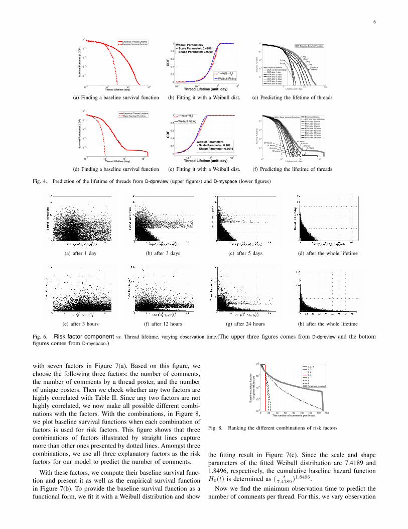
Fig. 4. Prediction of the lifetime of threads from D-dpreview (upper figures) and D-myspace (lower figures)

(a) after 1 day (b) after 3 days (c) after 5 days (d) after the whole lifetime

(e) after 3 hours (f) after 12 hours (g) after 24 hours (h) after the whole lifetime

Fig. 6. Risk factor component vs. Thread lifetime, varying observation time.(The upper three figures comes from D-dpreview and the bottomfigures comes from D-myspace.)

with seven factors in Figure 7(a). Based on this figure, wechoose the following three factors: the number of comments,the number of comments by a thread poster, and the numberof unique posters. Then we check whether any two factors arehighly correlated with Table II. Since any two factors are nothighly correlated, we now make all possible different combi-nations with the factors. With the combinations, in Figure 8,we plot baseline survival functions when each combination offactors is used for risk factors. This figure shows that threecombinations of factors illustrated by straight lines capturemore than other ones presented by dotted lines. Amongst threecombinations, we use all three explanatory factors as the riskfactors for our model to predict the number of comments.

With these factors, we compute their baseline survival func-tion and present it as well as the empirical survival functionin Figure 7(b). To provide the baseline survival function as afunctional form, we fit it with a Weibull distribution and show

0 20 40 60 80 100 120 140 16010−4

10−3

10−2

10−1

100

The number of comments per thread

Base

line

surv

ival

func

tion

for g

iven

risk

fact

ors

1, 3, 41, 33, 41, 4134Empirical survival

Fig. 8. Ranking the different combinations of risk factors

the fitting result in Figure 7(c). Since the scale and shapeparameters of the fitted Weibull distribution are 7.4189 and1.8496, respectively, the cumulative baseline hazard functionH0(t) is determined as ( t

7.4189 )1.8496.Now we find the minimum observation time to predict the

number of comments per thread. For this, we vary observation

7

0 20 40 60 80 100 120 140 16010−3

10−2

10−1

100

Number of comment (k)

Surv

ival

func

tion

S(k)

for a

giv

en ri

sk fa

ctor

s

Empirical number of comments1. number of comments2. time until the first comment3. #comm. by thread poster4. number of unique posters5. median of inter.comments time6. mean of inter.comments time7. variance of inter.comments time

4

31

(a) Selecting major risk factors

0 20 40 60 80 100 120 140 15010−3

10−2

10−1

100

Number of comments per thread (k)

Surv

ival

func

tion

S(k)

Empirical survival functionBaseline survival function S0(k)

(b) Baseline survival function

0 20 40 60 80 100 120 140 1600

0.2

0.4

0.6

0.8

1

Number of comments (k)

Prob

abilit

y

Failure function F(k): 1−exp(H0(k))

Weibull distribution fitting

Scale parameter: 11.1426 Shape parameter: 35.4320

(c) Fitting it with a Weibull distribution

Fig. 7. Predicting the number of comments of online discussion forum threads

(a) after 12 hours (b) after 1 day (c) after 3 days (d) after the whole lifetime

Fig. 10. Risk factor component vs. Number of comments per thread (varying observation time)

time as shown in Figure 9. This figure implies that when

0 20 40 60 80 100 120 14015010−3

10−2

10−1

100

Number of comments per thread (k)

Prob

abilit

y (lo

g sc

ale,

CC

DF)

Empirical number of commentsBSH w/o time limitationBSH after 6 hoursBSH after 12 hoursBSH after 24 hoursBSH after 2 daysBSH after 3 daysBSH after 4 daysBSH after 5 days

12 hours24 hours

6 hours

2 days

Fig. 9. Determining a minimum observation time

we use the information captured during the first 24 hours,the information for risk factors is not enough to predict thenumber of comments. The baseline survival function usingthe information observed for more than 2 days, however, isclose to the baseline survival function based on the wholeobservation. Thus, we could closely predict the number ofcomments of threads after observing the information on riskfactors for more than 2 days.

In Figure 10, we show risk factor component vs. the numberof comments per thread, varying observation time. Especially,Figure 10(d) shows the correlation between a hazard valueand the number of comments of a thread when all threadare dead. It clearly implies that while a thread with muchhazard has less comments, a thread with less hazard has muchcomments. In other words, as the values of risk factors of athread are increasing, the hazard of the thread is decreasingand its number of comments is increasing. Now let us visitFigure 10(a), 10(b), and 10(c). In Figure 10(a), we see thathazard values of almost all thread are high by positioning atthe right part of x-axis, but the hazard values are decreasingas the observation duration is getting longer in Figure 10(b)and 10(c).

Now we bring an application to predict threads, each of

which has more than 100 comments. We find that there are1,406 threads which have received more than 100 comments inD-dpreview and in Figure 11(a) we plot how many commentsthey received after one, two, and three days. After one day(two and three days) about 24% (56% and 73%) threadsamong 1,406 have more than 100 comments (respectively.)The following three figures show that how accurately we canpredict them and what the mean of comments of mis-predictedthreads after one, two, and three days. For instance, whenwe choose -200 as a threshold of risk factor component, wecan correctly find about 80% of threads after one day, basedon Figure 11(b). We additionally have mis-predictied threads(‘false positive’ threads), which the mean of their commentsis about 63. In a similar way, we can identify about 80% ofcorrect threads after two days based on Figure 11(c) whentaking -355 of a threshold. Remind that the mis-predictedthreads by our model are somehow popular even though theyare less popular than correctly identified ones, because ourapproach is based on the likelihood of the objective metric.Thus one who adopts our approach to model and predict anobjective metric of the popularity of a kind of online contentscan choose her threshold which satisfies her aim of predictionin terms of a precision and required observation time.

V. RELATED WORK

In this section, we briefly describe other literatures relatedto our work.• Survival analysis

Survival analysis [5] has been applied to various areas,such as bio-medical science, sociology, and epidemics[6], [7], [8], [9]. Among the methodologies for survivalanalysis, Cox proportional hazard regression model [3],which is a semi-parametric survival analysis methodol-ogy, has been widely used [10], [11], [12]. In this paper,we first adopted survival analysis and Cox proportional

8

0 50 100 150 1600

0.2

0.4

0.6

0.8

1

Number of comments per thread

CDF

During the whole lifetimeAfter 1 dayAfter 2 daysAfter 3 days

1 day

2 day

3 day

(a) CDF

−800 −600 −400 −200 00

0.2

0.4

0.6

0.8

1

!1x1 + !2x2 + !3x3

True

pos

itive

0

20

40

60

80

100

Mea

n nu

mbe

r of c

omm

ents

of fa

lse−

posi

tive−

thre

ads

(b) after 1 day

−800 −600 −400 −200 00

0.2

0.4

0.6

0.8

1

!1x1 + !2x2 + !3x3

True

pos

itive

0

20

40

60

80

100

Mea

n nu

mbe

r of c

omm

ents

of fa

lse−

posi

tive−

thre

ads

(c) after 2 days

−800 −600 −400 −200 00

0.2

0.4

0.6

0.8

1

!1x1 + !2x2 + !3x3

True

pos

itive

0

20

40

60

80

100

Mea

n nu

mbe

r of c

omm

ents

of fa

lse−

posi

tive−

thre

ads

(d) after 3 days

Fig. 11. Predicting the threads to have more than 100 comments. (In (b), (c), (d), straight lines are true positive values and dotted lines are mean values offalse negative values.)

regression approach to model and predict the popularityof online contents.

• Analysis on Threads and CommentsThe authors of [13], [14] analyzed the posts and com-ments of Slashdot. In detail, the authors of [13] explainedthe behaviors of inter-posts times with statistical mod-els and the authors of [14] focused on to analyze thedynamics of posts and users. There was a macroscopic-level analysis result, such as analysis on the averageviews and incoming links about posts and comments withweb logs in [15]. In [16], [17] the information of usercomments was used to understand user intention, and in[18] to find influential authors based on user commentswas investigated.

• Modeling Inter-Posting or Predicting PopularityIn [13], authors modeled post-comment-interval withfour different statistical models and they predicted in-termediate and long-term user activities. [2] proposed amethodology to predict the popularity of online contentsbased on a finding, the correlation of popularity betweenearly and later times. Then the authors proposed threeprediction models and validated them with Youtube andDigg datasets. In [19], authors built a co-participationnetwork among Digg users with comment information oftheir Digg dataset and proposed a method to predict thepopularity of online using an entropy measure explaininguser interest peak and the co-participation network. Ourwork is different in a point that we model and predict thepopularity of online contents with a set of explanatoryfactors by applying survival analysis and Cox propor-tional hazard model.

VI. CONCLUSION

In this paper, we proposed a methodology about macro-scopic prediction of the popularity of online contents, whichis to infer the likelihood that a content will attract a popularity.To model and predict an objective metric of the popularity ofonline contents we apply Cox proportional hazard regressionmodel for a set of given explanatory factors. We validatedour approach by predicting two kinds of popularity features(thread lifetime and the number of comments per thread) withtwo datasets from two discussion online forums. In the exper-iments, we showed that our approach successfully modeled apopularity metric with a set of risk factors and the popularitymetric was determined by the information represented by therisk factors.

REFERENCES

[1] M. Cha, A. Mislove, and K. P. Gummadi, “A measurement-drivenanalysis of information propagation in the flickr social network,” inWWW ’09: Proceedings of the 18th international conference on Worldwide web. New York, NY, USA: ACM, 2009, pp. 721–730.

[2] G. Szabo and B. A. Huberman, “Predicting the popularity of online con-tent,” Social Science Research Network Working Paper Series, November2008.

[3] D. R. Cox, “Regression models and life-tables,” Journal of the RoyalStatistical Society. Series B (Methodological), vol. 34, no. 2, pp. 187–220, 1972.

[4] W. Weibull, “A statistical distribution function of wide applicability,”Journal of Applied Mechanics, pp. 293–297, 1951.

[5] R. Schlittgen, “Survival analysis: State of the art,” ComputationalStatistics and Data Analysis, vol. 20, no. 5, pp. 592–593, November1995.

[6] A. R. Feinstein, Principles of Medical Statistics. Chapman & Hall/CRC,September 2001.

[7] D. G. Kleinbaum and M. Klein, Survival Analysis: A Self-Learning Text(Statistics for Biology and Health), 2nd ed. Springer, August 2005.

[8] A. Diekmann, M. Jungbauer-Gans, H. Krassnig, and S. Lorenz, “Socialstatus and aggression: a field study analyzed by survival analysis.” J SocPsychol, vol. 136, pp. 761–768, Dec 1996.

[9] S. Selvin, Survival Analysis for Epidemiologic and Medical Research(Practical Guides to Biostatistics and Epidemiology), 1st ed. CambridgeUniversity Press, March 2008.

[10] J. Heckman and B. Singer, “The identifiability of the proportional hazardmodel,” Review of Economic Studies, vol. 51, no. 2, pp. 231–41, April1984.

[11] P. B. Seetharaman and P. K. Chintagunta, “The proportional hazardmodel for purchase timing: A comparison of alternative specifications,”Journal of Business & Economic Statistics, vol. 21, no. 3, pp. 368–82,July 2003.

[12] T. M. Therneau, Modeling survival data: extending the Cox model, T. M.Therneau and P. M. Grambsch, Eds. New York, N.Y: Springer, 2000.

[13] A. Kaltenbrunner, V. Gomez, and V. Lopez, “Description and predictionof slashdot activity,” in LA-WEB ’07: Proceedings of the 2007 LatinAmerican Web Conference. Washington, DC, USA: IEEE ComputerSociety, 2007, pp. 57–66.

[14] A. Kaltenbrunner, V. Gomez, A. Moghnieh, R. Meza, J. Blat, andV. Lopez, “Homogeneous temporal activity patterns in a large onlinecommunication space,” in SAW, 2007.

[15] G. Mishne, “Leave a reply: An analysis of weblog comments.”[16] M. Hu, A. Sun, and E.-P. Lim, “Comments-oriented blog summarization

by sentence extraction,” in CIKM ’07: Proceedings of the sixteenth ACMconference on Conference on information and knowledge management.New York, NY, USA: ACM, 2007, pp. 901–904.

[17] B. Li, S. Xu, and J. Zhang, “Enhancing clustering blog documents byutilizing author/reader comments,” in ACM-SE 45: Proceedings of the45th annual southeast regional conference. New York, NY, USA: ACM,2007, pp. 94–99.

[18] N. Agarwal, H. Liu, L. Tang, and P. S. Yu, “Identifying the influentialbloggers in a community,” in WSDM ’08: Proceedings of the interna-tional conference on Web search and web data mining. New York, NY,USA: ACM, 2008, pp. 207–218.

[19] H. R. Salman Jamali, “Diggin digg: Comment mining, popularity pre-diction, and social network analysis,” George Mason University, Tech.Rep. GMU-CS-TR-2009-7, July 2009.