An Approach to Improve the Prediction of Injection...

An approach to improve the prediction of injection pressure in simulation technology

Ashwin Kumar. R.N, M.Senthil Murugan, Harindranath Sharma, Prasanta Mukhopadhyay, Sumanta Raha, Praful Soliya, Sadasivam G (From SABIC Research & Technology, Bangalore, India)

Abstract

Injection molding process simulation is a complex phenomenon wherein a thermoplastic material in melt state is injected into a cavity. The polymer melt replicates the details from the cavity and retains it as it solidifies and subsequently is ejected out of the mold. The Computer Aided Engineering (CAE) tools used for process simulation should be able to estimate the flow pattern, temperature distribution, shrinkage arising from material compressibility, viscous heating, pressure distribution, solidification, crystallization, fiber orientation, clamp force, etc. Despite many complexities arising from both material and molding process behavior, the CAE tools have evolved and matured to be reliable, accurate and useful in providing insightful details that can be used during product and process development. In some situations these tools still lack accuracy and overall reliability while analyzing some of the complex molding processes like thin wall molding, gas-assisted molding, etc. and needs to be studied to reduce these gaps and increase manufacturing predictability.

In this report a systematic approach and detailed steps to further improve the overall accuracy of CAE prediction is described. This covers critical aspects like measurement of mold surface temperature, melt temperature and reduce their uncertainty while using them as inputs in CAE. Through a detailed in-mold rheological study the influence of injection speed on pressure to mold the part is studied leading to derivation of molding window. The pressure loss that occurs in the machine screw barrel can be significant and is captured through an air-shot study. All these studies provide insights about the process and forms the basis for setting up the model in CAE, which is more representative of the actual process consisting of the part, material, the flow channels, initial temperature conditions of melt and mold. Using this approach and with the inclusion of improved characterization of resin’s viscosity in the CAE material model, we are able to predict the peak pressure in this representative tool within 10% of actual value for LEXAN™ LS1.

Introduction Recent industry trends indicate that injection-

molding applications have increasingly, become thinner and are being processed with highly filled resins. This demands development of newer analytical methods, material models and CAE solver capabilities for accurate process simulation. These are critical for predicting reliable results and assist in taking the right decisions on mold design and process optimization. In the simulation domain the plastic material has to be represented accurately for its

viscosity, Pressure, Specific-Volume, Temperature (p-V-T), thermal and mechanical behaviors. These inputs are used by the CAE solver to predict key results like flow pattern, pressure to fill, clamp force, shrinkage, cooling behavior, warpage, etc. and therefore are critical in obtaining good correlations between actual molding and CAE simulation results. The results from CAE simulation need to be accurate so that confident decisions may be taken on part, mold and process design. Commercial simulation softwares in the industry such as Autodesk Moldflow†, Moldex-3D†, Sigmasoft†, Cadmold†, Simpoe-Mold†, etc. are influential in plastics qualification process and used extensively during design stage. A good characterization of material is necessary to accurately simulate the injection molding process [1].

Several studies have evaluated the influence of various melt rheological parameters such as Cross-WLF (Williams-Landel-Ferry) parameters [1], pressure dependency of viscosity [2] [3], extensional viscosity [4], and junction loss parameters [5] on accuracy of simulations. When performing molding experiments for correlation study, once the process parameters are optimized, it is critical to allow the process to stabilize before extracting the data from the machine. Scientific molding principles should be employed to decide on the process settings [6]. The simulation model also influences the results from CAE. Depending on the type of elements used for modelling, the part and the feed system the pressure predicted and fill patterns will vary [7]. Modelling the part and feed system with 3D elements and accounting for flow through the machine nozzle in the simulation has been shown to result in better correlation of peak pressure between actual molding and CAE results [4]. Other factors such as mold deflection can also affect the correlation of actual molding and CAE [8], which are not considered in this study. A systematic method of performing molding experiments and CAE simulation for a correlation study is highlighted in this study and their results are reported for LEXAN™ LS1.

Experimental: Material Characterization

Several material properties have to be taken into consideration in order to achieve an accurate injection molding predictive simulation. In this section, the various material characterization techniques used are discussed. The resin used for this validation is commercial grade Polycarbonate (LEXAN™ LS1) with an MFR of 17.5 g/10 min at 300°C/ 1.2Kgf. It is an ultraviolet (UV) ray stabilized, transparent resin typically used for automotive lenses and various other applications. Some of the material attributes measured for this resin are: Specific heat (J/kg.K)

SPE ANTEC® Anaheim 2017 / 1411

as a function of temperature, (as per ASTM E1269), Thermal conductivity (W/mK) as a function of temperature, (as per ASTM D5930), Specific volume (cm3/gm) as a function of temperatures and pressures (as per Indirect dilatometry, Zoller technique [9], Elastic modulus (MPa, as per ASTM D638) and Coefficient of thermal expansion (mm/C, as per ASTM E831) and resin viscosity (Pa-sec. as per ASTM D3835).

It is well reported, that in addition to the conventional Cross-WLF parameters, the pressure dependence term, D3 in the Cross-WLF model is also critical for making an accurate estimation of the resin’s flow behavior under high injection pressures. SABIC has recently developed a methodology for measurement of D3, which will be reported in subsequent publications. Applying this methodology, the complete set of Cross-WLF parameters, estimated for the foresaid resin, is listed in Table 1.

Table 1 – Cross-WLF parameters for LEXAN LS1

n τ* (Pa)

D1 (Pa.s)

D2 (K)

D3 (K/Pa)

A1

Ã2 (K)

0.213 4.8E+5 5 E+09 417.15 1.8E-7 21.9 47.6

The Experimental Setup – Part, Mold and

Injection Molding Machine In this section, a detailed description of the

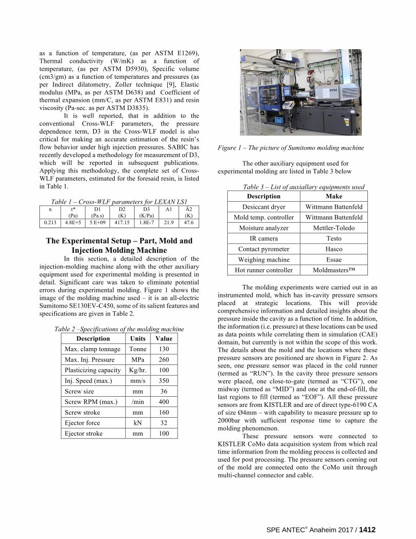
injection-molding machine along with the other auxiliary equipment used for experimental molding is presented in detail. Significant care was taken to eliminate potential errors during experimental molding. Figure 1 shows the image of the molding machine used – it is an all-electric Sumitomo SE130EV-C450, some of its salient features and specifications are given in Table 2.

Table 2 –Specifications of the molding machine

Description Units Value Max. clamp tonnage Tonne 130 Max. Inj. Pressure MPa 260 Plasticizing capacity Kg/hr. 100 Inj. Speed (max.) mm/s 350 Screw size mm 36 Screw RPM (max.) /min 400 Screw stroke mm 160 Ejector force kN 32 Ejector stroke mm 100

Figure 1 – The picture of Sumitomo molding machine

The other auxiliary equipment used for

experimental molding are listed in Table 3 below

Table 3 – List of auxiallary equipments used Description Make

Desiccant dryer Wittmann Battenfeld Mold temp. controller Wittmann Battenfeld

Moisture analyzer Mettler-Toledo IR camera Testo

Contact pyrometer Hasco Weighing machine Essae

Hot runner controller Moldmasters™

The molding experiments were carried out in an instrumented mold, which has in-cavity pressure sensors placed at strategic locations. This will provide comprehensive information and detailed insights about the pressure inside the cavity as a function of time. In addition, the information (i.e. pressure) at these locations can be used as data points while correlating them in simulation (CAE) domain, but currently is not within the scope of this work. The details about the mold and the locations where these pressure sensors are positioned are shown in Figure 2. As seen, one pressure sensor was placed in the cold runner (termed as “RUN”). In the cavity three pressure sensors were placed, one close-to-gate (termed as “CTG”), one midway (termed as “MID”) and one at the end-of-fill, the last regions to fill (termed as “EOF”). All these pressure sensors are from KISTLER and are of direct type-6190 CA of size Ø4mm – with capability to measure pressure up to 2000bar with sufficient response time to capture the molding phenomenon.

These pressure sensors were connected to KISTLER CoMo data acquisition system from which real time information from the molding process is collected and used for post processing. The pressure sensors coming out of the mold are connected onto the CoMo unit through multi-channel connector and cable.


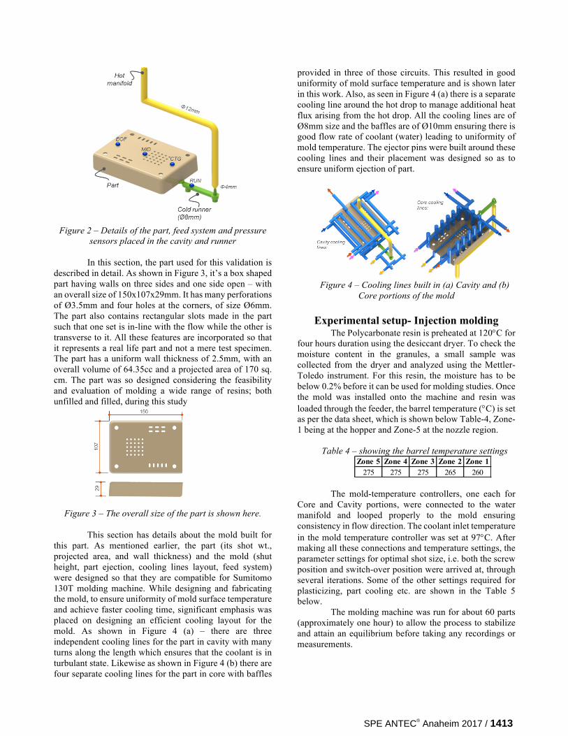
Figure 2 – Details of the part, feed system and pressure

sensors placed in the cavity and runner

In this section, the part used for this validation is described in detail. As shown in Figure 3, it’s a box shaped part having walls on three sides and one side open – with an overall size of 150x107x29mm. It has many perforations of Ø3.5mm and four holes at the corners, of size Ø6mm. The part also contains rectangular slots made in the part such that one set is in-line with the flow while the other is transverse to it. All these features are incorporated so that it represents a real life part and not a mere test specimen. The part has a uniform wall thickness of 2.5mm, with an overall volume of 64.35cc and a projected area of 170 sq. cm. The part was so designed considering the feasibility and evaluation of molding a wide range of resins; both unfilled and filled, during this study

Figure 3 – The overall size of the part is shown here.

This section has details about the mold built for this part. As mentioned earlier, the part (its shot wt., projected area, and wall thickness) and the mold (shut height, part ejection, cooling lines layout, feed system) were designed so that they are compatible for Sumitomo 130T molding machine. While designing and fabricating the mold, to ensure uniformity of mold surface temperature and achieve faster cooling time, significant emphasis was placed on designing an efficient cooling layout for the mold. As shown in Figure 4 (a) – there are three independent cooling lines for the part in cavity with many turns along the length which ensures that the coolant is in turbulant state. Likewise as shown in Figure 4 (b) there are four separate cooling lines for the part in core with baffles

provided in three of those circuits. This resulted in good uniformity of mold surface temperature and is shown later in this work. Also, as seen in Figure 4 (a) there is a separate cooling line around the hot drop to manage additional heat flux arising from the hot drop. All the cooling lines are of Ø8mm size and the baffles are of Ø10mm ensuring there is good flow rate of coolant (water) leading to uniformity of mold temperature. The ejector pins were built around these cooling lines and their placement was designed so as to ensure uniform ejection of part.

Figure 4 – Cooling lines built in (a) Cavity and (b)

Core portions of the mold

Experimental setup- Injection molding The Polycarbonate resin is preheated at 120°C for

four hours duration using the desiccant dryer. To check the moisture content in the granules, a small sample was collected from the dryer and analyzed using the Mettler-Toledo instrument. For this resin, the moisture has to be below 0.2% before it can be used for molding studies. Once the mold was installed onto the machine and resin was loaded through the feeder, the barrel temperature (°C) is set as per the data sheet, which is shown below Table-4, Zone-1 being at the hopper and Zone-5 at the nozzle region.

Table 4 – showing the barrel temperature settings

The mold-temperature controllers, one each for

Core and Cavity portions, were connected to the water manifold and looped properly to the mold ensuring consistency in flow direction. The coolant inlet temperature in the mold temperature controller was set at 97°C. After making all these connections and temperature settings, the parameter settings for optimal shot size, i.e. both the screw position and switch-over position were arrived at, through several iterations. Some of the other settings required for plasticizing, part cooling etc. are shown in the Table 5 below.

The molding machine was run for about 60 parts (approximately one hour) to allow the process to stabilize and attain an equilibrium before taking any recordings or measurements.

Zone 5 Zone 4 Zone 3 Zone 2 Zone 1275 275 275 265 260


Table 5 – Details of process settings used

Resin melt temperature measurement: The true resin melt temperature in the barrel can be different from what is set in the heater bands of the molding machine, due to shear heating, residence time, cycle time, etc. It is important to measure the true resin melt temperature as it can significantly influence the flow behavior and pressure in the cavity. The usual procedure for measurement of resin melt temperature is to retract injection unit back and purge the resin out of the nozzle. Then by inserting a temperature probe into the puddle of melt the temperature is recorded. Depending on the nozzle diameter of the machine and injection speed used during purging there could be considerable shear heating and temperature increase beyond what was set on machine barrel. This will be picked by the probe and can be wrongly concluded as melt temperature. In addition, we have used the 30/30 rule for melt temperature measurement, wherein the probe is heated to 30°C higher than the set temperature. Subsequently after purging, the probe was inserted into the melt puddle and observed for 30sec. – the lowest temperature seen was taken to be the true melt temperature and that was recorded.

Mold Temperature measurement- Again, to represent the model accurately in simulation (CAE) and to use the right process inputs, it is critical to record the mold surface temperature accurately. To achieve this, we have predefined six positions on the mold surfaces of both core and cavity inserts. At these locations, using surface pyrometer probe the temperature was measured and recorded as shown in Figure 5. The measured temperatures were used as an input for CAE simulations

Figure 5 – Shows the locations where the mold

surface temperature is measured

Principles of scientific molding

Applying principles of scientific injection molding, an in-mold rheology study was done using this box part and PC resin considered for this study. The detailed procedure for conducting an in-mold rheological study will not be discussed here. By performing such a study, the optimal injection speed for a given part-mold-

resin combination can be arrived. As seen in the below Table-6, the in-mold rheological study involved filling the part at different injection speeds. Part filling is carried out only until switch-over and no pack/holding phases were imposed. For each of these injection speed, the fill time (A) and peak pressure (C) is recorded (an average of three iterations is taken). The product of Fill time (Column A) and Peak pressure (Column C) was taken as Effective viscosity (Column D) of the resin at the given molding condition.

Table 6 – The details of in-mold rheology study

As shown in Figure 6 below, in-mold viscosity curve is obtained by plotting Effective viscosity (Column D) and Shear rate (Column B). This plot allows a visual assessment of the effect of variation of injection speed on cavity pressure. As we move to the right side on the curve, the injection speed increases and it could lead to excessive shear and gate blemish on the part. As we move to the left side on the curve, the injection speed is reducing, leading to viscosity build up during the flow. As any process is bound to have some natural variation, we would like to be in that portion of the curve where the change in effective viscosity (or pressure) in the cavity stays minimal due to this variation. In other words, any variation in shear rate (X1) should have minimal variation on effective viscosity (Y1) and the injection speed should be located in this regime.

Once the injection speed is derived, using the procedure described above, the settings for packing pressure and packing time is arrived at by performing gate freeze study. In such a study, keeping the pack pressure constant, pack duration was gradually increased and the part weight was recorded for every step. After a certain duration of pack time, the part weight becomes constant, reaching theoretical part weight. This is the time when the gate has frozen and packing the part beyond this time will increase the overall cycle time without any benefit to part quality. Likewise, prematurely stopping the packing time while the gate is still open will cause shrinkage variations and dimensional inconsistencies. Referring to the below

Description Units ValueInj. Screw dia. mm 36

Inj. Screw speed RPM 40Cooling time sec 30

Plasticising time sec 26Back pressure MPa 1.6

(A) (B) ( C ) (D)

#

Screw speed

mm/sec

Fill timesec

Shear Rate1/sec

Peak Pressure

MPa

Effective Viscosity

1 10 7.93 0.13 196.93 1562.252 20 3.96 0.25 161.00 637.883 30 2.64 0.38 155.60 411.254 35 2.27 0.44 155.17 351.465 40 1.98 0.50 157.00 311.176 50 1.59 0.63 160.47 254.517 75 1.06 0.94 172.03 182.358 100 0.80 1.25 182.47 145.619 125 0.64 1.56 190.27 121.96


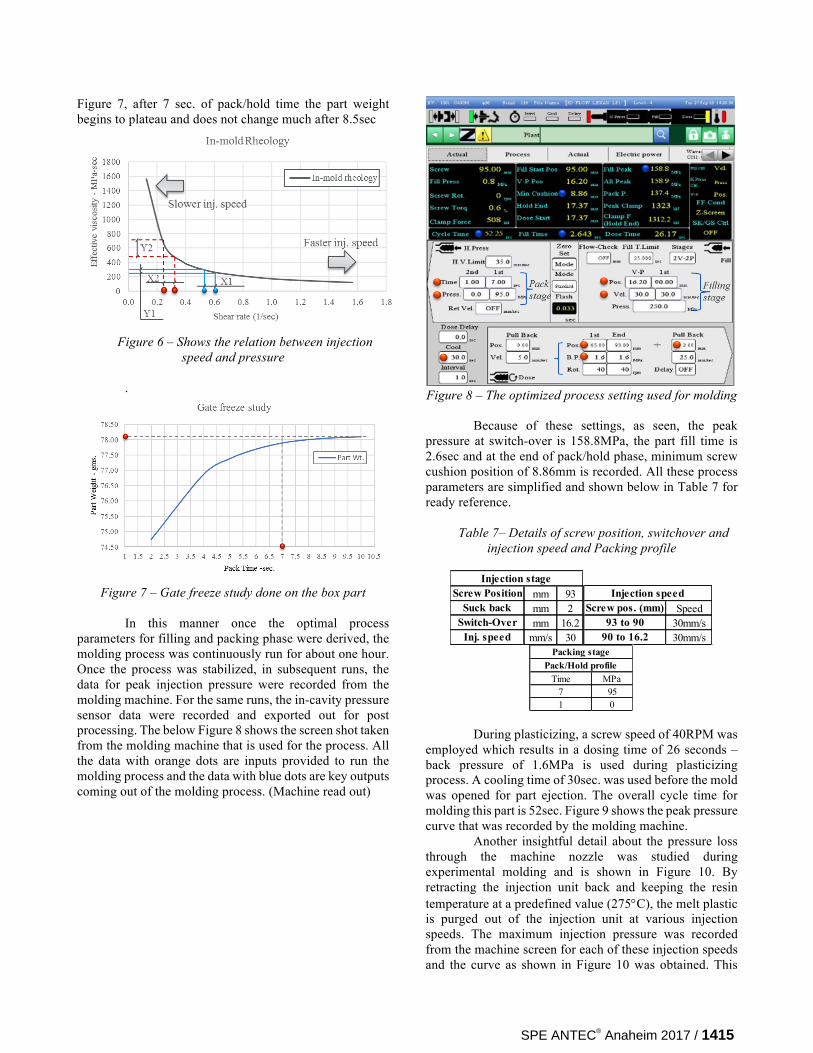
Figure 7, after 7 sec. of pack/hold time the part weight begins to plateau and does not change much after 8.5sec

Figure 6 – Shows the relation between injection

speed and pressure

.

Figure 7 – Gate freeze study done on the box part

In this manner once the optimal process parameters for filling and packing phase were derived, the molding process was continuously run for about one hour. Once the process was stabilized, in subsequent runs, the data for peak injection pressure were recorded from the molding machine. For the same runs, the in-cavity pressure sensor data were recorded and exported out for post processing. The below Figure 8 shows the screen shot taken from the molding machine that is used for the process. All the data with orange dots are inputs provided to run the molding process and the data with blue dots are key outputs coming out of the molding process. (Machine read out)

Figure 8 – The optimized process setting used for molding

Because of these settings, as seen, the peak

pressure at switch-over is 158.8MPa, the part fill time is 2.6sec and at the end of pack/hold phase, minimum screw cushion position of 8.86mm is recorded. All these process parameters are simplified and shown below in Table 7 for ready reference.

Table 7– Details of screw position, switchover and

injection speed and Packing profile

During plasticizing, a screw speed of 40RPM was

employed which results in a dosing time of 26 seconds – back pressure of 1.6MPa is used during plasticizing process. A cooling time of 30sec. was used before the mold was opened for part ejection. The overall cycle time for molding this part is 52sec. Figure 9 shows the peak pressure curve that was recorded by the molding machine.

Another insightful detail about the pressure loss through the machine nozzle was studied during experimental molding and is shown in Figure 10. By retracting the injection unit back and keeping the resin temperature at a predefined value (275°C), the melt plastic is purged out of the injection unit at various injection speeds. The maximum injection pressure was recorded from the machine screen for each of these injection speeds and the curve as shown in Figure 10 was obtained. This

Screw Position mm 93Suck back mm 2

Switch-Over mm 16.2Inj. speed mm/s 30

Injection stage

Screw pos. (mm) Speed93 to 90 30mm/s

90 to 16.2 30mm/s

Injection speed

Time MPa7 951 0

Pack/Hold profilePacking stage


shows the pressure drop that can occur in the machine nozzle as a function of injection speed. This will indeed be a function of the nozzle geometry design and the polymer material – in this case, it is a Ø3mm nozzle. At the injection speed used to mold this part i.e:30mm/sec. the pressure loss through the nozzle was seen to be 34MPa for this resin.

Figure 9 – Shows the peak pressure trace captured

from the molding machine

Figure 10 – Pressure loss through the machine nozzle

Simulation In this section, the development of an accurate and

a true representative CAE simulation model will be discussed. In this validation study, the part and the feed system, which includes the gate, cold runner and the hot drop, were all modelled using 3D elements. Considerable effort has been spent to understand the mesh sensitivity of the model on some of the key results like pressure and flow pattern before deciding it.

To include the pressure loss that occurs in the machine screw barrel, the front portion of the machine nozzle was measured using a Co-ordinate Measuring machine (CMM) and a CAD geometry was developed. This nozzle geometry is included into the feed system model and finally they are integrated with the part geometry – all these are meshed using 3D elements, thus forming the basis for FE meshed model. The Figure 11 below shows the simulation model where the part, the feed system along with the front portion of the injection barrel is captured, all

using 3D elements. The overall element count in the discretized model considering all these aspects and refinement is about 2.5million Typical to any production mold, vents will be provided for the air to escape out during part filling. Referring to the mold that was used here, the vent locations and their sizes were measured precisely and recorded. These, as measured from the mold, have a width of 6mm, thickness of 0.03mm and are provided on the parting plane at six distinct locations. This is replicated in the simulation model using “modeling of vents” option available in Moldflow† MPI CAE software. Capturing this detail in the simulations is of importance as it represents the real world mold by being able to capture the additional resistance present in the system. The air present inside the mold will have to evacuate only through these vents during the part-filling phase. The process settings recorded during experimental molding study were used as inputs for CAE simulation in the same manner and are show below in Table 8.

Figure 11 – Simulation model used in CAE, includes

the front portion of the injection unit

Table 8 - Shows the inputs used for mold and melt temperature, the filling and packing controls and cooling

time used in simulation model

Mold surface temp. Deg. C 95Melt Temperature Deg. C 275

Absolute ram speed Ram Pos. (mm) Ram speed (mm/s)90 3016.2 30

Filling Control

Screw start pos. (mm) 93Switch-Over pos.(mm) 16.2

Cooling time (s) 30

Duration (s) Pressure (MPa)0 957 951 0

Packing Pressure v/s Time


Results and Discussion

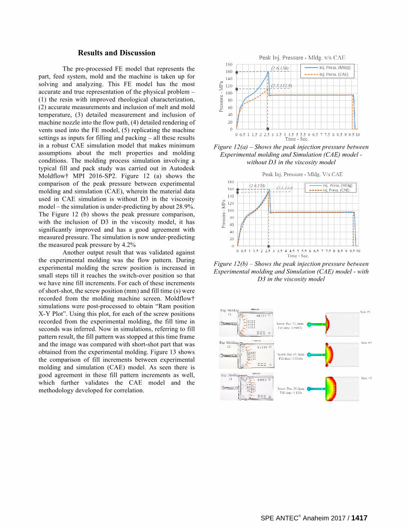
The pre-processed FE model that represents the part, feed system, mold and the machine is taken up for solving and analyzing. This FE model has the most accurate and true representation of the physical problem – (1) the resin with improved rheological characterization, (2) accurate measurements and inclusion of melt and mold temperature, (3) detailed measurement and inclusion of machine nozzle into the flow path, (4) detailed rendering of vents used into the FE model, (5) replicating the machine settings as inputs for filling and packing – all these results in a robust CAE simulation model that makes minimum assumptions about the melt properties and molding conditions. The molding process simulation involving a typical fill and pack study was carried out in Autodesk Moldflow† MPI 2016-SP2. Figure 12 (a) shows the comparison of the peak pressure between experimental molding and simulation (CAE), wherein the material data used in CAE simulation is without D3 in the viscosity model – the simulation is under-predicting by about 28.9%. The Figure 12 (b) shows the peak pressure comparison, with the inclusion of D3 in the viscosity model, it has significantly improved and has a good agreement with measured pressure. The simulation is now under-predicting the measured peak pressure by 4.2% Another output result that was validated against the experimental molding was the flow pattern. During experimental molding the screw position is increased in small steps till it reaches the switch-over position so that we have nine fill increments. For each of these increments of short-shot, the screw position (mm) and fill time (s) were recorded from the molding machine screen. Moldflow† simulations were post-processed to obtain “Ram position X-Y Plot”. Using this plot, for each of the screw positions recorded from the experimental molding, the fill time in seconds was inferred. Now in simulations, referring to fill pattern result, the fill pattern was stopped at this time frame and the image was compared with short-shot part that was obtained from the experimental molding. Figure 13 shows the comparison of fill increments between experimental molding and simulation (CAE) model. As seen there is good agreement in these fill pattern increments as well, which further validates the CAE model and the methodology developed for correlation.

Figure 12(a) – Shows the peak injection pressure between

Experimental molding and Simulation (CAE) model - without D3 in the viscosity model

Figure 12(b) – Shows the peak injection pressure between Experimental molding and Simulation (CAE) model - with

D3 in the viscosity model


Figure 13 – Shows the fill pattern comparison between experimental molding (left images) and

simulation (CAE)

Conclusions The approach used here while conducting

molding experiments has been systematic and done with a scientific approach. It has been observed and documented that the key to achieving successful correlation between experimental molding and simulation (CAE) lies with characterization of material behavior, accurate measurement and recordings of the key process parameters like injection speed, melt temperature and modeling the complete resin flow path. In the simulation domain, it is important to develop the FE model that truly represents the real world scenario as much as possible. In this manner, the results of validation show that good correlation can be established in injection molding simulation for predicting peak pressure. This in turn will enable the design team to take decision confidently during part, mold and process development.

References [8] [1] D. A. Okonski, "An injection molding simulation

validation study: material property versus simulation accuracy," in SPE ANTEC, 2013.

[2] Gal Sherbelis and Chris Friedl, "The importance of pressure dependent viscosity and contraction pressure losses to injection molding CAE analysis," in ANTEC, 1996.

[3] M. Mahishi, "Material characterization for thin wall molding," in ANTEC - Processing, 1998.

[4] Erik Foltz, Matt Dachel, Franco S. Costa and Paul Brincat, "Accounting for pressure dependent and elongational viscosities to improve injection pressure predictions in mold filling analysis," in SPE ANTEC, Indianapolis, 2016.

[5] Guojun Xu and Kurt W. Koelling, "Study of Cavity Pressure and its Prediction during Injection Molding," in ANTEC, 2003.

[6] S. Kulkarni, "Scientific Processing and Scientific Molding," in Robust Process Development and Scientific Molding - Theory and Practice, Hanser Publishers, 2010.

[7] Matthew J. Jaworski and Zhongshuang Yuan, "Theoritical and experimental comparison of the four major types of mesh currently used in CAE injection molding simulation software," in ANTEC, 2003.

[8] U Vietri, A. Sorrentino, V. Speranza and R. Pantani, "Improving the Predictions of Injection Molding Simulation Software," in Polymer Engineering & Science, 2011.

† Any brands, products or services of other companies referenced in this document are the trademarks, service marks and/or trade names of their respective holders.


An Approach to Improve the Prediction of Injection...

Documents

Transcript of An Approach to Improve the Prediction of Injection...