An Application-Level Network Mapper · am eliorer des communications collectives) et non de d...
33
HAL Id: inria-00071214 https://hal.inria.fr/inria-00071214 Submitted on 23 May 2006 HAL is a multi-disciplinary open access archive for the deposit and dissemination of sci- entific research documents, whether they are pub- lished or not. The documents may come from teaching and research institutions in France or abroad, or from public or private research centers. L’archive ouverte pluridisciplinaire HAL, est destinée au dépôt et à la diffusion de documents scientifiques de niveau recherche, publiés ou non, émanant des établissements d’enseignement et de recherche français ou étrangers, des laboratoires publics ou privés. An Application-Level Network Mapper Arnaud Legrand, Frédéric Mazoit, Martin Quinson To cite this version: Arnaud Legrand, Frédéric Mazoit, Martin Quinson. An Application-Level Network Mapper. [Research Report] RR-5792, INRIA. 2006. <inria-00071214>
Transcript of An Application-Level Network Mapper · am eliorer des communications collectives) et non de d...

HAL Id: inria-00071214https://hal.inria.fr/inria-00071214
Submitted on 23 May 2006
HAL is a multi-disciplinary open accessarchive for the deposit and dissemination of sci-entific research documents, whether they are pub-lished or not. The documents may come fromteaching and research institutions in France orabroad, or from public or private research centers.
L’archive ouverte pluridisciplinaire HAL, estdestinée au dépôt et à la diffusion de documentsscientifiques de niveau recherche, publiés ou non,émanant des établissements d’enseignement et derecherche français ou étrangers, des laboratoirespublics ou privés.
An Application-Level Network MapperArnaud Legrand, Frédéric Mazoit, Martin Quinson
To cite this version:Arnaud Legrand, Frédéric Mazoit, Martin Quinson. An Application-Level Network Mapper. [ResearchReport] RR-5792, INRIA. 2006. <inria-00071214>
ISS
N 0
249-
6399
ISR
N IN
RIA
/RR
--57
92--
FR
+E
NG
ap por t de r ech er ch e
Thème NUM
INSTITUT NATIONAL DE RECHERCHE EN INFORMATIQUE ET EN AUTOMATIQUE
An Application-Level Network Mapper
Arnaud Legrand — Frédéric Mazoit — Martin Quinson
N° 5792
Janvier 2006


Unité de recherche INRIA LorraineLORIA, Technopôle de Nancy-Brabois, Campus scientifique,
615, rue du Jardin Botanique, BP 101, 54602 Villers-Lès-Nancy (France)Téléphone : +33 3 83 59 30 00 — Télécopie : +33 3 83 27 83 19
An Application-Level Network Mapper
Arnaud Legrand∗ , Frederic Mazoit† , Martin Quinson‡
Theme NUM — Systemes numeriquesProjets Mescal, MC2 et Algorille
Rapport de recherche n�
5792 — Janvier 2006 — 29 pages
Abstract: Modern grid platforms present a much more complex interconnection topologythan classical super-computers or clusters. Information about this topology is critical tonetwork-aware applications, such as a grid scheduler optimizing communication times, orsuch as data replication managers.
This paper presents a theoretical framework and the corresponding tool for automaticallydiscovery of network topology. The goal is not to discover the physical layout of machinesinterconnections, but to construct a synthetic view of the effects of the topology as per-ceived by an application. Among other things, this requires that performance of concurrenttransfers can be assessed.
Our work uncovers an original mathematical model that arises from the formalization ofthe topology discovery problem, for which we propose an algorithm. We prove that when theunderlying graph is a constellation of trees (i.e., a set of trees whose roots are interconnectedby a complete clique), our algorithm produces a valid solution. We then extend the algorithmto other cases. We present some preliminary evaluation results obtained with the SimGrid
simulator.
Key-words: Grid computing, network topology, communication performance prediction
∗ ID, UMR 5132 (CNRS–INPG–INRIA–UJF), Grenoble, France. [email protected]† LIP, UMR 5668 (CNRS–ENS-Lyon-UCBL–INRIA), Lyon, France. [email protected]‡ LORIA, UMR 7503 (UHP–CNRS–INPL–INRIA–Nancy2), Nancy, France. [email protected]
Decouverte de topologie au niveau applicatif
Resume : Cet article presente un outil de decouverte automatique de la topologie du reseau.Son objectif est d’evaluer les performances de transferts concurrents (par exemple pourameliorer des communications collectives) et non de decouvrir le schema d’interconnexionphysique des machines (ce qui pourrait servir a diagnostiquer des problemes de configurationreseau).
Un modele mathematique permettant la formalisation du probleme est introduit. Graceaux outils analytiques resulants, nous proposons un premier algorithme pour resoudre ceprobleme. Nous demontrons sous certaines hypotheses la validite de cet algorithme lorsqu’ilest possible de construire une solution formant une constelation d’arbres (c’est-a-dire unensemble d’arbres dont les racines sont interconnectees par une clique complete). Nousetendons ensuite cet algorithme pour lui permettre de traiter certains cas ou l’introductiond’autres formes de cycles dans la solution est necessaire. Des resultats preliminaires obtenussur simulateur sont egalement proposes.
Mots-cles : Calcul distribue a grand echelle, topologie de reseaux, prediction de perfor-mances de communications

An Application-Level Network Mapper 3
1 Introduction
Grids are a type of parallel and distributed systems that result from the sharing and ag-gregation of geographically distributed resources between several organizations [4]. Unlikeclassical parallel machines, Grids present dynamic, heterogeneous and often non-dedicatedcapacities. Gathering accurate, up to date and relevant informations about them is then avery challenging issue, which has to be addressed before developing network-aware applica-tions on the grid.
Most of the previous work in the grid community such as the NWS [9] or RPS [2] projectsfocused on acquiring quantitative knowledges like network bandwidth and latency, or CPUload. More qualitative informations such as the network topology are however crucial toachieve tasks such as host placement or collective communications performance prediction.Since our goal is to permit the advent of network-aware applications and not to developa network administration tool, the most relevant information is not the actual physicalinterconnection schema but a mean to estimate the performance of concurrent transfers.
The topology reconstruction problem is a classical subject in the networking communityand has already received a lot of attention. The most classical tools to that extend (likeping or traceroute) provide too limited information to detect the network bottlenecksoccurring in the case of concurrent data streams. The use of tools providing sufficientinformation such as pathchar or the SNMP protocol are often restricted to trusted usersfor security reasons since the involved protocols can be used to conduct Deny Of Serviceattacks or reveal information considered as commercial secret by network owners. Thislimitation makes those approaches unsuited to the grid context since the platform is mostoften constituted by several distinct organizations diverging in their security policies. It isthus very difficult or even impossible to be given privileges beyond the simple user ones onthe whole platform.
Some recent work focus on the design of new measurement scheme usable without anyspecific privileges. In [7], the authors presents a methodology based only on regular packetexchanges. Unfortunately, the obtained view of the platform does not fulfill our needs. Itfocuses on the physical interconnection topology and the description of the path followedby the packets while our goal is to identify the interferences between concurrent streams.These two notions are very close, but do not necessary match. If, using this methodology,two paths are reported to be independent (i.e., they do not share any network element),it is clear that data streams using these paths cannot interfere, but the contrary is notnecessary true. Indeed, if the shared section is over-dimensioned and able to carry bothstreams without impacting on their performance, we want our tool to report the paths asindependent. This goal’s divergence makes this approach unusable directly in our context.
The closest project to our goal is ENV (Effective Network View [8]). It can reconstructa view of the network topology focusing on interactions of concurrent data streams withoutrequiring any specific privileges on the platform. In [5], we study the possibility of usingthis tool to automatically place the classical NWS grid monitoring tool. Unfortunately, forefficiency reasons, ENV only report a hierarchical view of the network whereas classical grid
RR n�
5792

4 Legrand & Mazoit & Quinson
testbeds are often constituted of wide area constellation of local area networks. The tree-based view offered by ENV may thus lack some lateral connections. For example, the nodesof a clusters will be represented as leafs of the tree, and some intra-cluster communicationfacilities may be omitted by ENV.
This paper introduces a tool called ALNeM (Application-Level Network Mapper), whichis designed to gather network topology informations useful to network-aware applications.Its goal is not to help administrators to monitor their network and diagnostic bottlenecksor failure points, but rather to give other applications the ability to predict the networkperformance of data streams. The rest of this article is organized as follows: Section 2 detailsour goals and introduces the used model. Thanks to the mathematical tools presented inSection 3, we give an algorithm in Section 4. We prove (under some assumptions) thatwhen the underlying graph is forming a constellation of trees (i.e., a set of trees whichroots are interconnected by a complete clique), our algorithm builds an equivalent graph.We then extend this algorithm to handle some of the cases where cycles are mandatoryin the solution. Section 5 suggests a solution to collect the informations needed for thisreconstruction. Experimental results obtained on simulator are presented in Section 6. Theproofs of lemmas and theorems are placed in appendix of this paper.
2 The ALNeM project
Before detailing the ALNeM methodology, we should clarify its goals and the model used.First of all, ALNeM does not try to discover the network topology at a router-level andcannot be used network administration tool. It aims at providing a view of the network thatis expressive and accurate enough to enable applications running on grid computing plat-forms to optimize their performances (communication pattern, load-balancing, deployment,. . . ). Knowing whether two concurrent data streams interfere is mandatory to achieve thisgoal.
Note that obtaining a perfect view including all routers, link capacities and routing in-formation may be possible thanks to some tools like pathchar and the SNMP protocol.Nevertheless, even when forgetting about the induced security problems that impede theiruse in our context, such a low-level view is generally not sufficient to determine the inter-ference of two concurrent data streams. Indeed, interference is a dynamic feature of thenetwork and depends on the load on each link which is very hard to monitor. Moreover thegraph representing the router-level topology is generally very large and thus hard to handle.A suitable network view for network-aware applications optimization should therefore havemoderate size while modeling lifelike interferences. For that reason we aim at proposing aminimalist view of the network.
INRIA

An Application-Level Network Mapper 5
2.1 Model used
The relevant information is more qualitative than quantitative since other tools like theNWS [9] can be used to acquire the quantitative data. At first, the network view can thusbe modeled by a simple non-weighted graph.
Definition 1. A routed graph G = (V, E, r) is a connected non-oriented graph and a routingfunction r : V × V → V . r(u, v) is the node to follow to reach v from u. Therefore foreachu, v ∈ V : (u, r(u, v)) ∈ E.
Given u, v ∈ V , the notation(u −→
Gv)
represents the ordered set of vertices encountered
in the graph G on the route from u to v (u and v are respectively the first and the lastelement of this set). This set obviously depends on the routing function r used.
The most important machines in our context are the ones on which applications can beexecuted without specific privileges. This excludes the machines of the network infrastruc-ture such as firewalls and routers, which may be omitted from our representation.
Definition 2. The set of the platform nodes ( i.e., the hosts on which user applications canbe deployed) is noted H.
As stated previously, the searched information is the possible performance impact thatdata streams occurring at the same time imply on each other. In other words, we needto predict whether the bandwidth between two given machines is affected by a transferoccurring between two other machines at the same time, or if the two streams can coexistwithout mutual interference. The most natural way to model this notion of interferencebetween the stream (AB) and (CD) in a routed graph is to consider the intersection of theroute between A and B and the one between C and D. If this intersection is non-empty,then (AB) and (CD) do interfere on each other.
Definition 3. Given a, b, c, d ∈ H, the fact that the path (ab) interfere with (cd) in the Ggraph is denoted (ab) ��G (cd). This is defined by the following relation:
(ab) ��G (cd)⇐⇒(a −→
Gb)∩
(c −→
Gd)6= ∅
The non-interference in the graph G between (ab) and (cd) is denoted (ab) �G (cd), anddefined by:
(ab) �G (cd)⇐⇒ ¬((ab) ��G (cd)
)
This defines the so-called theoretical interference (by opposition to the measured inter-ference introduced in the next section). This relation is also noted ��th when the graph onwhich it applies is given by the context. These definitions trivially lead to the followinglemma (since the set intersection is a symmetric relation):
Lemma 1 (��th is a symmetric relation).
∀a, b, c, d ∈ H, (ab) ��th (cd)⇔ (cd) ��th (ab).
RR n�
5792

6 Legrand & Mazoit & Quinson
Remark 1. The equivalence (ab) ��th (cd) ⇔ (ba) ��th (cd) is not true when the routing isnon-symmetric, i.e., when (ab) 6= (ba).
2.2 Measurement methodology
As explained in the previous section, the key notion on which we base our network view isthe interference. We now define more precisely how to measure this information.
Definition 4. Let G = (V , E, r) be the routed graph representing the physical topology
with V the set of all existing hosts (including the one of the network infrastructure such as
routers), E the links connecting them and r the paths followed by data streams.
The routing r used in G depends on the configuration of each element of V and is thusonly locally known. Even if the graph G reflects a physical reality, it is rarely actuallyknown. Issues like faulty protocol implementations and configuration errors may causerouting inconsistencies such as asymmetric or changing paths, and even loops. According to[6], such situations are quite common in existing wide area networks.
Under those conditions, the simplest way to know whether a transfer impacts anotherone (without relying on methodology whose use may be restricted to privileged users) is toconduct a direct experiment by comparing the usual bandwidth to the one achieved whenthe second connection is saturated.
Definition 5. Given four nodes a, b, c et d, the bandwidth between a and b when no extratraffic is injected between c and d is denoted bw(ab). The bandwidth between a and b whenthe connection between c and d is saturated is denoted bw�cd(ab).
This allows to define an interference notion based on the comparison of these two values:if their ratio equals 0.5, that means that the two data streams fairly share a limiting networkfacility. If this ratio equals 1, (cd) have no impact on (ab). We use thresholds to account forthe measurement errors and the perturbations dues to the external load.
Definition 6. We consider that (cd) impacts on (ab) if and only if
bw�cd(ab)
bw(ab)< 0.7
We denote that case with the following notation (ab) ��mes (cd) (mes standing for measured).
Definition 7. If this ratio is greater than 0.9, we consider that the transfers do not interfere.This is denoted by (ab) �mes (cd).
A ratio between 0.7 and 0.9 is supposed to result of measurement error, and to imply thatthe experiment should be conducted again. Those ratio are the same as the ones determinedempirically by the authors of the ENV project [8].
INRIA

An Application-Level Network Mapper 7
Lemma 2 (��mes is not a symmetric relation). That is to say:
∃a, b, c, d ∈ H /((ab) ��mes (cd)
)∧ ¬
((cd) ��mes (ab)
)
Proof. Figure 1 presents a counter-example to the symmetry of the ��mes relation.
10 Mo/s 100 Mo/s 100 Mo/sa c b d
Figure 1: Counter example to the symmetry of the ��mes relation.
In that case, the result of the measurements may be at the same timebw�cd(ab)
bw(ab) < 0.7
andbw�ab(cd)
bw(cd) > 0.9 since the link (ab) is limited to 10 Mb/s on the (ac) segment. Its impact
on (cd) (on which the bandwidth tends to 100 Mb/s) is thus undetectable.
We can notice however that the paths (ab) and (cd) in this counter-example do share
a common link of G. Moreover, the impact of (ab) on (cd) do exist, even if it remainsundetectable to the conducted measurements. This leads to the symetrization of the relationin order to match the ��th notion.
Definition 8. We consider that (ab) and (cd) interfere if and only if (ab) impacts (cd) or(cd) impacts (ab). This is denoted by (ab) ��rl (cd) ( rl standing for real). We have:
(ab) ��rl (cd)⇐⇒
{(ab) ��mes (cd)
(cd) ��mes (ab)(or) ⇐⇒
{bw�cd(ab)
bw(ab) < 0.7bw�ab(cd)
bw(cd) < 0.7(or)
In the opposite case, we consider that the paths do not interfere with each other, whichis denoted by (ab) �rl (cd).
By construction, the relation ��rl is symmetric, and (ab) ��rl (cd) ⇐⇒ ¬ (ab) �rl (cd). Itis thus possible to store the value of this relation for all nodes in a four dimensional matrixdefined as follows:
Definition 9. Let I(H, ��rl) be the interference matrix between all elements of the H set, asimplied by the relation ��rl:
I(H, ��rl)(a, b, c, d) =
{1 if (ab) ��rl (cd)
0 else
RR n�
5792

8 Legrand & Mazoit & Quinson
2.3 Problem statement
As explained is section 2, we are looking for an easy-to-use view of the network. Therelation between the measured interference ��rl and the physical interconnection graph G ismuch more complicated than the relation between their theoretical counterparts ��th and G.Therefore, we propose to identify ��rl and ��th as the same notion and to look for a routedgraph mimicking the real interferences. Thanks to the notations introduced in the previoustwo sections, we can now define more formally the problem which ALNeM aims to solve:
Definition 10. InterferenceGraph: Given H and I(H, �� eG), find a routed graph G =(V, E, r) such that:
H ⊂ V ;
I(H, �� eG) = I(H, ��G) ;
|V | is minimal.
The idea is to look for an abstract graph G mimicing the effects of G with regard to theinterferences between streams. This allows the users to manipulate G to acquire informationson G. In order to simplify its use, we have to keep the size of G as small as possible.
The first natural question that arises about this optimization problem is the following:“Given an arbitrary interference matrix, is it always possible to find a graph G so thatI(H, �� eG) = I(H, ��G)?”. The answer to this question is positive as stated in the followingtheorem.
Theorem 1. For all H and I(H, �� eG), there exists a graph G = (V, E, r) such that:
{H ⊂ V ;
I(H, �� eG) = I(H, ��G) ;
Nevertheless the size of the graph built in the proof (detailed in Appendix A) is ex-ponential in the size of H. Therefore, the second question that arises about the hardnessof our problem concerns its feasibility in a polynomial size: “Given an arbitrary interfer-ence matrix, is there a routed graph of reasonable size (i.e. polynomially bounded) so thatI(H, �� eG) = I(H, ��G)?”. We still do not know the answer to this question, which prevents usto state properly the decision problem associated to InterferenceGraph. In Section 4,we analyze some particular situations where we are able to find a solution such that H =V .
3 Mathematical tools
This section presents some mathematical tools for the theoretical study the Interference-
Graph. They constitute the framework needed to manage the algorithm presented in thenext section.
INRIA
An Application-Level Network Mapper 9
3.1 Hypotheses
We assume in this paper that the graph G respects the following hypotheses:
Hypothesis 1 (routing consistency). ∀(a, b, c) ∈ V :
c ∈
(a −→
eG
b
)=⇒
(a −→
eG
b
)∩
(a −→
eG
c
)=
(a −→
eG
c
)
This hypothesis indicates that the routing algorithm used in G does not present weirdinconsistencies. If a vertex c is on the path connecting a to b, the packets transiting from ato b follow the same path on the beginning of their trip than the ones transiting from a toc. The contrary would imply for example that the machine a uses an host ρ as gateway, andthat ρ routes the packets for b through c while a can connect to c directly without using ρ.
Remark 2. Using the routing definition, this hypothesis gives: ∀(a, b, c) ∈ V :
c ∈
(a −→
eG
b
)=⇒
(a −→
eG
b
)∩
(c −→
eG
b
)=
(c −→
eG
b
)
Hypothesis 2 (routing symmetry). ∀(a, b) ∈ V :
(a −→
eG
b
)=
(b −→
eG
a
)
This hypothesis indicates that the routing is symmetric.We know that both of these hypotheses may be violated on Internet since all imaginable
routing inconsistency exists in the reality [6]. However, as we would like to get an abstractview of the network where those local difficulties have disappeared, we will try in the fol-lowing to build a routed graph where these hypotheses hold and will therefore suppose thatthey hold true when needed.
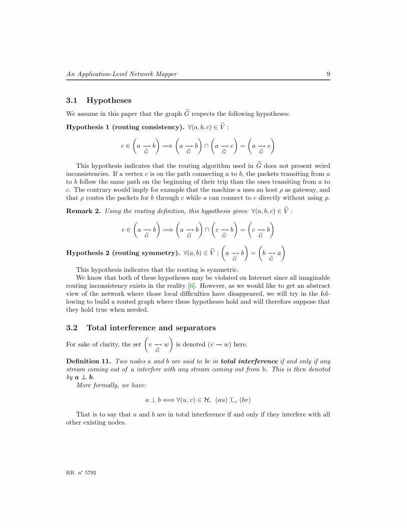
3.2 Total interference and separators
For sake of clarity, the set
(v −→
eG
w
)is denoted (v −→ w) here.
Definition 11. Two nodes a and b are said to be in total interference if and only if anystream coming out of a interfere with any stream coming out from b. This is then denotedby a ⊥ b.
More formally, we have:
a ⊥ b⇐⇒ ∀(u, v) ∈ H, (au) ��rl (bv)
That is to say that a and b are in total interference if and only if they interfere with allother existing nodes.
RR n�
5792
10 Legrand & Mazoit & Quinson
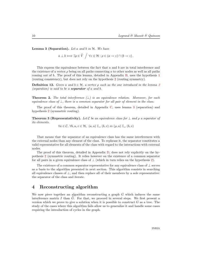
Lemma 3 (Separation). Let a and b in H. We have
a ⊥ b⇐⇒ ∃ρ ∈ V/∀z ∈ H : ρ ∈ (a −→ z) ∩ (b −→ z) .
This express the equivalence between the fact that a and b are in total interference andthe existence of a vertex ρ being on all paths connecting a to other nodes as well as all pathscoming out of b. The proof of this lemma, detailed in Appendix B, uses the hypothesis 1(routing consistency), but does not rely on the hypothesis 2 (routing symmetry).
Definition 12. Given a and b ∈ H, a vertex ρ such as the one introduced in the lemma 3(separation) is said to be a separator of a and b.
Theorem 2. The total interference (⊥) is an equivalence relation. Moreover, for eachequivalence class of ⊥, there is a common separator for all pair of element in the class.
The proof of this theorem, detailed in Appendix C, uses lemma 3 (separation) andhypothesis 2 (symmetric routing).
Theorem 3 (Representativity). Let C be an equivalence class for ⊥ and ρ a separator ofits elements.
∀a ∈ C, ∀b, u, v ∈ H, (a, u) ��rl (b, v)⇔ (ρ, u) ��rl (b, v)
That means that the separator of an equivalence class has the same interferences withthe external nodes than any element of the class. To rephrase it, the separator constitutes avalid representative for all elements of the class with regard to the interactions with externalnodes.
The proof of this theorem, detailed in Appendix D, does not rely explicitly on the hy-pothesis 2 (symmetric routing). It relies however on the existence of a common separatorfor all pairs in a given equivalence class of ⊥ (which in turn relies on the hypothesis 2).
The existence of a common separator representative for any equivalence class of ⊥ servesas a basis to the algorithm presented in next section. This algorithm consists in searchingall equivalence classes of ⊥, and then replace all of their members by a sole representative:the separator of the class and iterate.
4 Reconstructing algorithm
We now piece together an algorithm reconstructing a graph G which induces the sameinterference matrix I than G. For that, we proceed in several steps. We first present aversion which we prove to give a solution when it is possible to construct G as a tree. Thestudy of the cases where this algorithm fails allow us to generalize it and handle some casesrequiring the introduction of cycles in the graph.
INRIA
An Application-Level Network Mapper 11
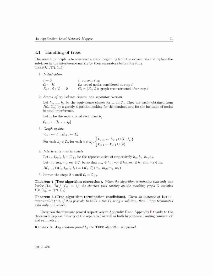
4.1 Handling of trees
The general principle is to construct a graph beginning from the extremities and replace thesub-trees in the interference matrix by their separators before iterating.Tree(H, I(H, ��rl))
1. Initialization
i← 0 i: current stepCi ← H Ci: set of nodes considered at step iEi ← ∅ ; Vi ← ∅ Gi = (Ei, Vi): graph reconstructed after step i
2. Search of equivalence classes, and separator election
Let h1, . . . , hp be the equivalence classes for ⊥ on Ci. They are easily obtained fromI(Ci, ��rl) by a greedy algorithm looking for the maximal sets for the inclusion of nodesin total interference.
Let lj be the separator of each class hj .
Ci+1 ← {l1, . . . , lp}
3. Graph update
Vi+1 ← Vi ; Ei+1 ← Ei
For each hj ∈ Ci, for each v ∈ hj ,
{Ei+1 ← Ei+1 ∪ {(v, lj)}
Vi+1 ← Vi+1 ∪ {v}
4. Interference matrix update
Let lα, lβ, lγ , lδ ∈ Ci+1 be the representative of respectively hα, hβ, hγ , hδ.
Let mα, mβ , mγ , mδ ∈ Ci be so that mα ∈ hα, mβ ∈ hβ, mγ ∈ hγ and mδ ∈ hδ.
I(Ci+1, ��)(lα, lβ, lγ , lδ
)= I (Ci, ��)
(mα, mβ , mγ , mδ
)
5. Iterate the steps 2-4 until Ci = Ci+1.
Theorem 4 (Tree algorithm correction). When the algorithm terminates with only oneleader ( i.e., ∃n
/ ∣∣Cn∣∣ = 1), the shortest path routing on the resulting graph G satisfies
I(H, ��G) = I(H, ��rl).
Theorem 5 (Tree algorithm termination conditions). Given an instance of Inter-
ferenceGraph, if it is possible to build a tree G being a solution, then Tree terminateswith only one leader.
These two theorems are proved respectively in Appendix E and Appendix F thanks to thetheorem 3 (representativity of the separator) as well as both hypotheses (routing consistencyand symmetry);
Remark 3. Any solution found by the Tree algorithm is optimal.
RR n�
5792

12 Legrand & Mazoit & Quinson
Indeed, the theorem 3 (representativity of the separator) allows to use any element ofthe class as separator. That way, no new vertex is introduced by the algorithm. The set ofvertices in G is thus restricted to H, and G is then clearly optimal.
4.2 Handling of cliques
When, at a given step i of the Tree algorithm, there is no remaining interference betweenthe elements of Cn, it is naturally impossible to find two nodes being in total interference.When this occurs, the algorithm fails to construct the wanted graph.
The intuitive solution in that case, consisting in connecting all the representatives ofeach class in a clique manner, leads to a valid solution. The following theorem expressesthis more formally.
Theorem 6. (Clique handling validity) If there exists a step i of Tree so that ∀ai, ui, bi, vi ∈Ci, (ai, ui) � (bi, vi), then the graph G connecting all pairs of elements in Ci satisfiesI(H, ��G) = I(H, ��rl) when the shortest path routing algorithm is used.
This extension allows the algorithm to handle tree constellations, i.e., graphs formed byseveral distinct trees whose roots are all interconnected by a clique.
Remark 4. The solutions found by this extension, when they exist, are also optimal sinceno new vertex is introduced.
4.3 Cycle handling
By application of the theorem 5 (Tree algorithm terminaison condition), we know that ifthe algorithm fails to end with a connected graph, then no tree mimicing the interferencesgiven by I exists. In particular, it is necessary to introduce cycles in G to find a solution.
We now present an extension of the algorithm handling the interference matrices inducedby some graph G containing cycles. Since graphs containing cycles have weakest propertiesthan trees, the chosen approach is more pragmatic and the solution is less generic.
We assume that the Tree algorithm were applied to group in the same connected set allelements in total interference, but that the connectivity of the builded graph is only partial.We are thus at a step i of the algorithm where there is no lα, lβ ∈ Ci so that lα ⊥ lβ.
The main idea of our algorithm to handle this situation is to find two nodes close to eachother on a cycle, cut the cycle between them so that the Tree algorithm can go further,and then reintroduce the cycle by reconnecting those two points afterward.
This approach induces two different difficulties. We first have to detect two such pointsusing only the informations provided by the interference matrix. We then have to find away to reintroduce the cycle afterward.
In our algorithm, the cycle is cut between the two vertices having the most interferencein the matrix, i.e., between the two vertices a and b maximizing the set {u, v : au �� bv}. Itis possible to split the vertices set in four sub-sets I1, I2, I3 and I4 defined as following:
INRIA

An Application-Level Network Mapper 13
I1 ={u ∈ Ci : a ∈ (b −→ u) and b 6∈ (a −→ u)
}
I2 ={u ∈ Ci : a 6∈ (b −→ u) and b ∈ (a −→ u)
}
I3 ={u ∈ Ci : a 6∈ (b −→ u) and b 6∈ (a −→ u)
}
I4 ={u ∈ Ci : a ∈ (b −→ u) and b ∈ (a −→ u)
}
The hypothesis 1 implies trivially that I4 = {a, b} because if there existed an element u
differing of a and b in I4, we would have the following contradictory case:a
bu
b
a
I3
I2
1I
βα
Figure 2: Split of the vertices set to handle cycles.
Using the hypothesis 1 (routing consistency), the general organization of the underlyinggraph is therefore as depicted in Figure 2. We introduce a point α separating the sets{u ∈ Ci : b ∈ (a −→ u)} and {u ∈ Ci : b 6∈ (a −→ u)}. Likewise, the point β is constructedwith regard to b. Note that these two points may not belong to H and are difficult to detectbut are well-defined.
We now have to determine the three sets I1, I2 and I3 based on the information containedby the interference matrix. If we knew those three sets, we would be able to order the nodesalong the main cycle and the corresponding matrix slice on (a, b) would then have a veryparticular configuration (see Figure 3). Indeed, when u ∈ I1 and v ∈ I1 then (au) �� (bv),explaining that the upper left part of the table is filled of 1.
Finding a nodes permutation so that the matrix slice on (a, b) is organized as in Figure 3can be done by sorting topologically the strongly connected components of the graph fromwhich this slice is the adjacency matrix. Such a reordering then gives the wanted split of theCi elements into I1, I2 and I3 based only on the informations contained in the interferencematrix.
The next challenge is the reconnection of the graphs obtained by recursion on those sub-sets. Since we split the cycle on two positions (between a and b, and between α and β), wehave to reconnect it on each of them. Reconnecting a and b simply needs the addition of anew edge. In order to reconnect the cycle between α and β, we first have to find the closestvertices from the splitting point.
RR n�
5792

14 Legrand & Mazoit & Quinson
I3
I2
1Ibα βa
b
α
β
a
1 1?0 01
1 01 }
}}
v
u
Figure 3: Interference matrix slice on (a, b) after reordering.
We know that the first step of the Tree recursion on I1 will find elements being in totalinterference since we broke the cycle and thus created strings around a and α. Since Tree
was unable to find elements in total interference at the previous step, those strings are theonly existing subtrees. It is moreover easy to differentiate them since one of them containsa.
By symmetry on I3 and b, we deduce that the reconnection should occur between one ofthe point of the connected set created by the first iteration of Tree on I1 which does notcontain a on one side, and one of the point from the connected set resulting of Tree on I3
on the other side. The choice between the possible multiple candidates is done by selectingthe points Sα and Sβ having the more interferences with the other points of Ci (using theintuition that points presenting more interferences should be close in the graph).
After identification of Sα and Sβ being the sets border where the reconnection shouldoccur, this reconnection is achieved by executing the algorithm recursively on the set I2 ∪{Sα, Sβ}.
This provides us with an algorithm able to handle some cases where cycles are mandatory.This is however not a complete generalization since the graph G by our algorithm doesnot necessarily respect all the constraints expressed by the interference matrix. Amongstother reasons, this is due to the fact that the decisions are taken using only a slice ofthe interference matrix to decide how to build G, disregarding the possibly contradictoryinformations presented elsewhere in the matrix. Theorem 1 suggests that no such greedyalgorithm can solve this problem.
5 Collecting the needed data
We now tackle the way the needed data about the interference on the platform may bemeasured. This is a technically challenging issue which may reveal time-consuming andthus deserve optimizations.
INRIA

An Application-Level Network Mapper 15
5.1 Intuitive algorithm
The simplest way to collect those informations resides in |H|4 steps (for each quadruplet(a, b, c, d) ∈ H4), each of them consisting in:
1. Measure the bandwidth on (ab) (denoted bw(ab)) ;
2. Measure the bandwidth on (ab) when the link (cd) is saturated (denoted bw�cd(ab)) ;
3. Compute the ratio.
The steps 1. and 2. must last long enough to let the network stabilize. We first have towait long enough after an experiment before starting the next one to avoid any perturbationand we also have to wait for the link (cd) to be actually saturated before conducting thesecond step. Those delays forbid to reasonably test more than ten quadruplets per minute
on a possibly wide area network. The execution of this algorithm lasts thus |H|4
10 minutes,which represents about 10 days when |H| = 20. This solution is thus foredoomed by lack ofextensibility.
5.2 Optimizations
In order to speed up the process, ALNeM conducts the experiments in parallel, thanks toindependent links. Since they do not interfere with each other, it is possible to saturateseveral of them at the same time. That way, when a new link is tested, it is not testedagainst only one link, but against all links currently saturated.
If the saturation of the new link implies a performance decrease on one of the linkpreviously saturated, we report the interference in the matrix and stop the last saturation. Ifthe saturation of the new link does not imply any performance modification of the previouslysaturated link, we continue by adding another saturation.
The more independent saturation we achieve at the same time, the less the whole mea-surement process lasts. In order to predict the probably independent links and increase theparallelism, a preliminary step constructs a first guess of the topology using traceroute.As discussed before, the result of this step does not perfectly fit our needs since this method-ology does not allow to capture all interferences, but those informations reveal precious toguide our measurement algorithm.
The speedup offered by this optimization naturally depends on the G characteristics.The worst case is when all links interfere with each other, forbidding any parallelization.The best case is when no link interfere with any other, allowing a complete parallelization.In this case, our algorithm needs only 2|H|2 steps to complete (about one hour for 20 nodes).Since typical testbeds are constituted of a wide area constellation of local area networks,which are often trees, we think that this optimization may lead to important speedups.
Furthermore, this algorithm needing a centralized clock, the measurements are synchro-nized by a specific node called maestro. The position of this node in the network doeshowever not impact the results.
RR n�
5792

16 Legrand & Mazoit & Quinson
6 Mapping example
This section introduces a prototype of ALNeM developed in the SimGrid [1] simulator.The presented results were obtained by feeding the simulator with a topology generated byTiers [3], and running ALNeM within the simulator without providing it any preliminaryinformation about this topology. The Figure 4 depicts at the same time the “real” topologyas provided to SimGrid (4(a)), the data provided to ALNeM (4(b)) and the G graph re-constructed by ALNeM (4(c)). Figure 5 depicts different steps of ALNeM’s reconstructionalgorithm in that case.
0
32
42
5
6
1
8
10
16
100
101
102
103
104
20
105
106
107
108
109
22
11
12
14
19
110
111112
113
114
39
115
116
117
118
119
120
121
122
123
124
34
125
126
127
128129
36
13
15
130
131
132
133
134
31
135
136
137
138
13946
60
140
141
142
143
144
40
145
146
147
148
149
4
7
150
151
152
153
154
47
155
156
157
158
159
44
18
75
160
161
162
163
164
58
17
80
170
171 172
173
174
52
175
176
177
178179
59
65
70
180
181
182
183
184
53
2
27
3
51
21
25
28
85
95
23
24
29
26
90
30
35
33
37
38
9
45
41
50
55
56
57
6162
63
64
66
67
68
69
71
72
73
74
76
77
78
79
81
82
83
84
86
87
88
89
91
92
93
94
96
9798
99
(a) Topology used ( eG). (b) Initial data (plus I��rl
). (c) ALNeM result (G).
Figure 4: Example of graph reconstruction.
7 Conclusion and future work
In this paper, we present an network mapping framework called ALNeM (Application-LevelNetwork Mapper). It is meant to capture a macroscopic and qualitative view of the networktopology suited for network-aware applications. It does not try to discover neither thenetwork physical interconnection schema nor the path followed by the packets. This wouldbe interesting for administrators wanting to auscultate their networks, but would be lessrelevant in our context. This tool does not either try to precisely determine the end-to-endbandwidth since other tools like NWS already retrieve those measurements.
The information captured by ALNeM is a graph accounting for the possible interference(in term of performance) between concurrent data streams. Data movement on (ab) and(cd) can occur at the same time without impacting on the performance if and only if theshortest paths on (ab) and (cd) have an empty intersection in this graph. If not, they doimpact on each other.
INRIA

An Application-Level Network Mapper 17
Figure 5: Successive steps of the reconstruction algorithm.
RR n�
5792

18 Legrand & Mazoit & Quinson
The reconstruction of this representation is a well-defined problem that we call Inter-
ferenceGraph. Even if we have not been able to prove it yet, we think that this problemis NP–complete. We propose an algorithm that builds the optimal solution whenever theunderlying graph is a constellation of trees (i.e., several trees whose roots are interconnectedby a clique). We also propose an extension of the algorithm able to handle some cases inwhich other forms of cycle are mandatory in the builded graph. An accurate study of thisextension’s limits will be tackled in future work.
We would like to enrich our model in the future to predict the bandwidth threshold abovewhich the performance interference occures. We implicitly assumed that two concurrentstreams are enough to detect any bottleneck in the network. This is however not the case,and some resources may become limiting (thus creating an interference) only when sharedby three or more streams. We could take this fact into account by introducing a notion ofN-interference when N streams are mandatory to reveal the bottleneck. Another solutionwould be to tag each separator by a threshold representing the bandwidth needed to makethe resource it represents limiting.
Finally, we present how ALNeM measure the data needed to the application of thisalgorithm and some possible optimizations. In order to ensure ALNeM’s applicability onlarge platforms, we plan to increase in future work the parallelism achieved by a finer analysisof the results provided by traceroute or ping.
In order to limit the number of hosts involved in each mapping (and thus reduce thetime needed), we also plan to study how to merge preexisting topology. It may implyto conduct some extra measurements beyond the one needed to get each sub-topology, butwould probably allow to come up with a recursive algorithm able to map networks containinga large number of hosts efficiently. Likewise, an iterative algorithm able to add a new node toa previously computed topology is needed to avoid the recomputation of the whole topologywhen a new node appears or disappears.
More generally, we think that the measurement step may be greatly optimized by agreater interaction with the reconstruction step allowing to schedule the tests depending onthe current knowledge about the topology.
To that concern, it may be very interesting to integrate ALNeM to a network monitoringinfrastructure such as NWS. This would allow to conduct the more intrusive measurementswhen regular users do not use the network. It would also ensure the automatic detection ofthe structural changes by conducting regular tests to verify that previous results still matchthe current situation. Those results would be beneficial both to NWS itself to improve itsconfiguration and to client applications.
INRIA
An Application-Level Network Mapper 19
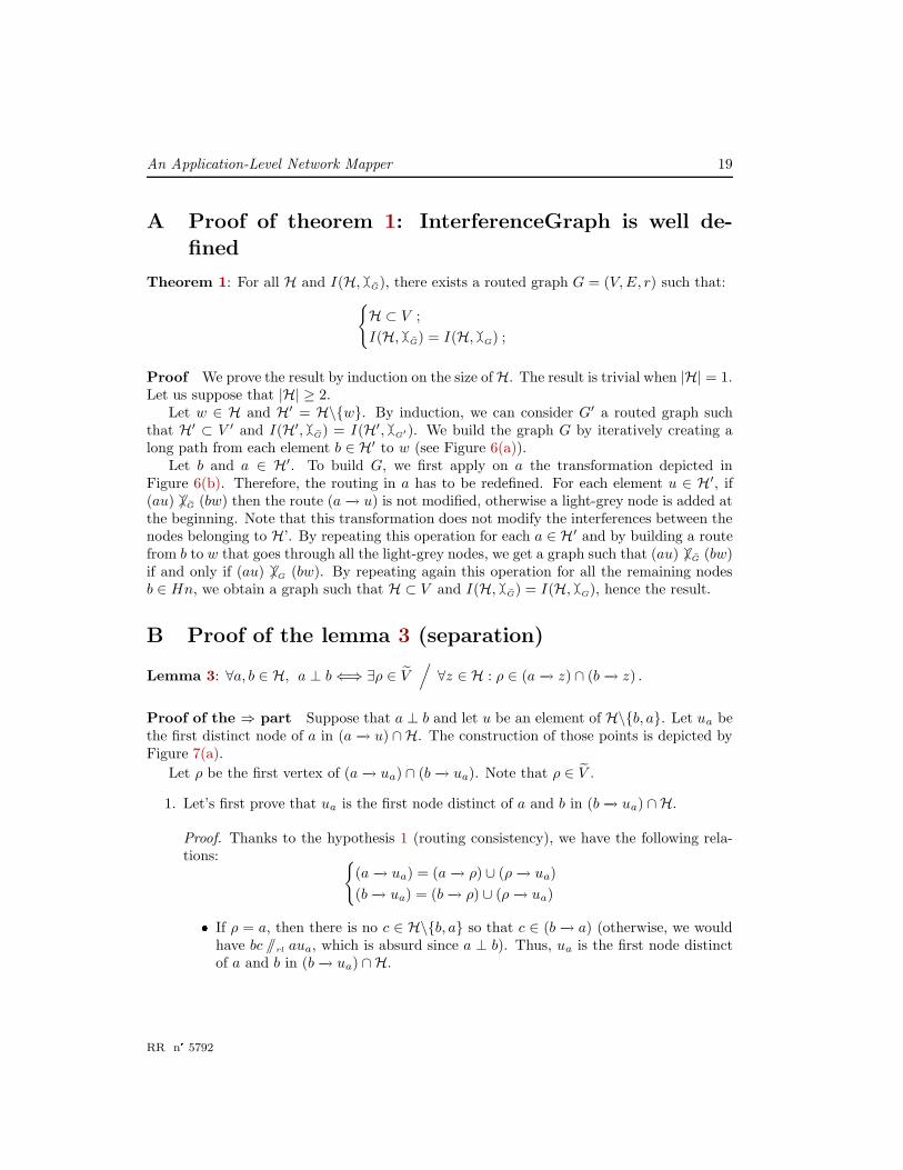
A Proof of theorem 1: InterferenceGraph is well de-
fined
Theorem 1: For all H and I(H, �� eG), there exists a routed graph G = (V, E, r) such that:
{H ⊂ V ;
I(H, �� eG) = I(H, ��G) ;
Proof We prove the result by induction on the size ofH. The result is trivial when |H| = 1.Let us suppose that |H| ≥ 2.
Let w ∈ H and H′ = H\{w}. By induction, we can consider G′ a routed graph suchthat H′ ⊂ V ′ and I(H′, �� eG) = I(H′, ��G
′). We build the graph G by iteratively creating along path from each element b ∈ H′ to w (see Figure 6(a)).
Let b and a ∈ H′. To build G, we first apply on a the transformation depicted inFigure 6(b). Therefore, the routing in a has to be redefined. For each element u ∈ H′, if(au) 6�� eG (bw) then the route (a −→ u) is not modified, otherwise a light-grey node is added atthe beginning. Note that this transformation does not modify the interferences between thenodes belonging to H’. By repeating this operation for each a ∈ H′ and by building a routefrom b to w that goes through all the light-grey nodes, we get a graph such that (au) 6�� eG (bw)if and only if (au) 6��G (bw). By repeating again this operation for all the remaining nodesb ∈ Hn, we obtain a graph such that H ⊂ V and I(H, �� eG) = I(H, ��G), hence the result.
B Proof of the lemma 3 (separation)
Lemma 3: ∀a, b ∈ H, a ⊥ b⇐⇒ ∃ρ ∈ V/∀z ∈ H : ρ ∈ (a −→ z) ∩ (b −→ z) .
Proof of the ⇒ part Suppose that a ⊥ b and let u be an element of H\{b, a}. Let ua bethe first distinct node of a in (a −→ u) ∩ H. The construction of those points is depicted byFigure 7(a).
Let ρ be the first vertex of (a −→ ua) ∩ (b −→ ua). Note that ρ ∈ V .
1. Let’s first prove that ua is the first node distinct of a and b in (b −→ ua) ∩ H.
Proof. Thanks to the hypothesis 1 (routing consistency), we have the following rela-tions: {
(a −→ ua) = (a −→ ρ) ∪ (ρ −→ ua)
(b −→ ua) = (b −→ ρ) ∪ (ρ −→ ua)
� If ρ = a, then there is no c ∈ H\{b, a} so that c ∈ (b −→ a) (otherwise, we wouldhave bc �rl aua, which is absurd since a ⊥ b). Thus, ua is the first node distinctof a and b in (b −→ ua) ∩ H.
RR n�
5792

20 Legrand & Mazoit & Quinson
b
a
wH′
(a) Reasoning by induction onthe size of H.
a
b
w
a
(b) Transforming each node.
Figure 6: Sketch of the proof of Theorem 1.
INRIA
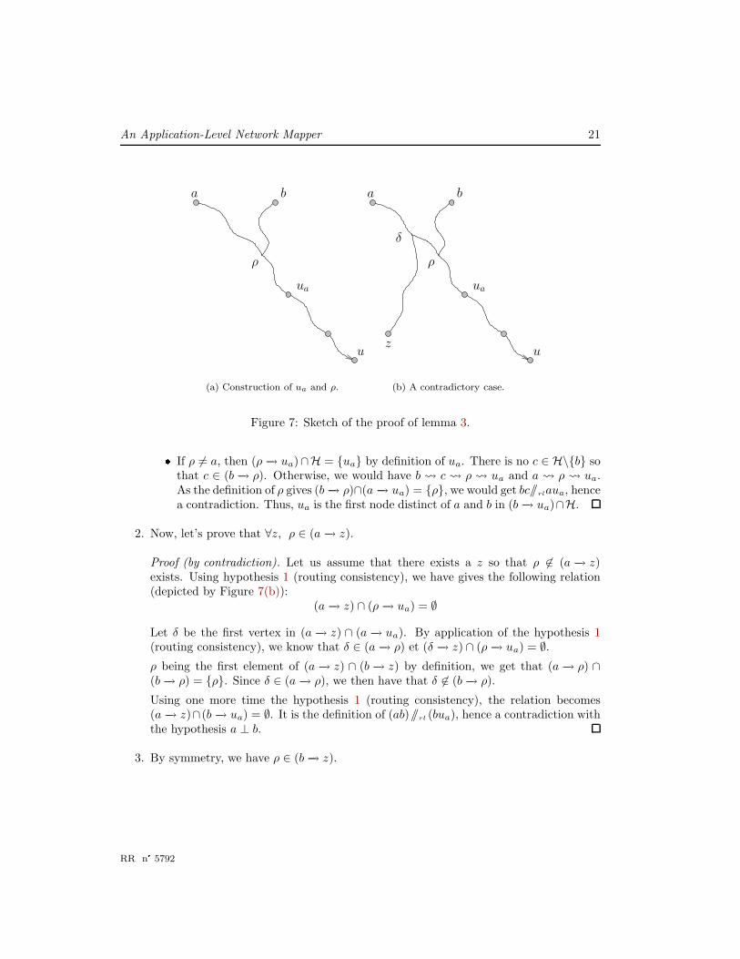
An Application-Level Network Mapper 21
ba
ua
u
ρ
(a) Construction of ua and ρ.
z
δ
ba
ua
u
ρ
(b) A contradictory case.
Figure 7: Sketch of the proof of lemma 3.
� If ρ 6= a, then (ρ −→ ua)∩H = {ua} by definition of ua. There is no c ∈ H\{b} sothat c ∈ (b −→ ρ). Otherwise, we would have b c ρ ua and a ρ ua.As the definition of ρ gives (b −→ ρ)∩(a −→ ua) = {ρ}, we would get bc�rlaua, hencea contradiction. Thus, ua is the first node distinct of a and b in (b −→ ua)∩H.
2. Now, let’s prove that ∀z, ρ ∈ (a −→ z).
Proof (by contradiction). Let us assume that there exists a z so that ρ 6∈ (a −→ z)exists. Using hypothesis 1 (routing consistency), we have gives the following relation(depicted by Figure 7(b)):
(a −→ z) ∩ (ρ −→ ua) = ∅
Let δ be the first vertex in (a −→ z) ∩ (a −→ ua). By application of the hypothesis 1(routing consistency), we know that δ ∈ (a −→ ρ) et (δ −→ z) ∩ (ρ −→ ua) = ∅.
ρ being the first element of (a −→ z) ∩ (b −→ z) by definition, we get that (a −→ ρ) ∩(b −→ ρ) = {ρ}. Since δ ∈ (a −→ ρ), we then have that δ 6∈ (b −→ ρ).
Using one more time the hypothesis 1 (routing consistency), the relation becomes(a −→ z)∩ (b −→ ua) = ∅. It is the definition of (ab)�rl (bua), hence a contradiction withthe hypothesis a ⊥ b.
3. By symmetry, we have ρ ∈ (b −→ z).
RR n�
5792

22 Legrand & Mazoit & Quinson
This leads to the wanted result:
∀z ∈ H :
{ρ ∈ (a −→ z)
ρ ∈ (b −→ z)
Proof of the ⇐ part This implication is trivial. Let ρ ∈ V be so that:
∀z ∈ H :
{ρ ∈ (a −→ z)
ρ ∈ (b −→ z)
This leads to ∀u, v ∈ H, ρ ∈ (a −→ u) ∩ (b −→ v), and thus to (au) �� (bv).Thus a ⊥ b.
C Proof of theorem 2 (⊥ is an equivalence relation)
Theorem 2. The total interference (⊥) is an equivalence relation. Moreover, for eachequivalence class of ⊥, there is a common separator for all pair of element in the class.
In order to prove that ⊥ is an equivalence relation, we naturally have to prove its reflexiveproperty (which done in lemma 4), its symmetric property (lemma 5) and its transitiveproperty (lemma 6). This last lemma also prove the existence of a common separator acrossthe whole equivalence class.
Lemma 4 (⊥ is reflexive). That is to say ∀a ∈ H, a ⊥ a.
Proof. For all a, u, v ∈ H, (a −→ u) ∩ (a −→ v) = {a} 6= ∅. Thus (au) �� (av), which is thedefinition of a ⊥ a.
Lemma 5 (⊥ is symmetric). That is to say ∀a, b ∈ H, a ⊥ b⇔ b ⊥ a.
Proof. This is trivially given by the fact that �� is symmetric by construction.
Lemma 6 (⊥ is transitive). Given three nodes a, b, c ∈ H, if(a ⊥ b
)∧
(b ⊥ c
)then this
nodes have a common separator and thus a ⊥ c.
Proof. Let a, b, c ∈ H be so that a ⊥ b and b ⊥ c.Let u ∈ H. Let ua be the first node distinct of a in (a −→ u)∩H. Let ρ be the first node
in (a −→ ua) ∩ (b −→ ua) and σ be the first node in (b −→ ua) ∩ (c −→ ua).ρ is thus a separator of a and b while σ is a separator of b and c (this, as well as theexistence of ρ and σ, is given by application of the lemma 3). These definitions also implythat ρ ∈ (b −→ c) and σ ∈ (b −→ c).
1. Let’s proof that ρ = σ by contradiction.
INRIA

An Application-Level Network Mapper 23
Proof. Let’s assume that ρ 6= σ. Two cases are possible: (b→ ρ→ σ → c) or (b→ σ → ρ→ c).
(a) Let’s assume that (b→ ρ→ σ → c) (Relation denoted A�
).
i. Let’s show that (a −→ ρ) ∩ (c −→ σ) = ∅ is impossible since it would imply(ab) � (cua).
Proof.
The definition of σ imply:b
c
σ ua
With A�
, this becomes:ρb
c
σ ua
With the definition of σ, this becomes:a
ρb
c
σ ua
With the hypothesis 2 (symmetry), this leads to:a
ρb
c
σ ua
Since we supposed ρ 6= σ, this gives (b→ ρ→ a) ∩ (c→ σ → ua) = ∅.A rewriting of each parts of ∩ leads to: (b −→ a) ∩ (c −→ ua) = ∅.Thus, (ab) � (cua), which is contradictory with b ⊥ c.
ii. Let’s show that (a −→ ρ) ∩ (c −→ σ) 6= ∅ is also impossible in that case.
Proof. Let δ be the first element of (a −→ ρ) ∩ (c −→ σ).
The definition of δ as well as A�
lead to:b
ρ σ uaδc
a
By definition of ρ, this leads to:ρ σ uaδc
a
Thus, ρ is placed before σ on (b −→ ua) ∩ (c −→ ua), which is contradictory ifρ 6= σ since σ is the first element of this set by definition.
(i) and (ii) being the two only possible cases, the relation A�
is contradictory.
(b) By symmetry, (b→ σ → ρ→ c) is also impossible.
Both cases being impossible, the proposition ρ 6= σ is contradictory, and thus ρ =σ.
2. σ is thus at the same time the first element of (a −→ ua) ∩ (b −→ ua) and of (b −→ ua) ∩(c −→ ua).
Since σ is the first element of (a −→ ua) ∩ (b −→ ua), we have: σ ua
a
b
RR n�
5792
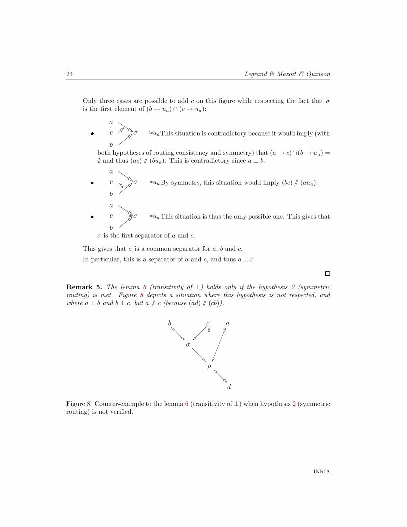
24 Legrand & Mazoit & Quinson
Only three cases are possible to add c on this figure while respecting the fact that σis the first element of (b −→ ua) ∩ (c −→ ua):
� c σ ua
a
b
This situation is contradictory because it would imply (with
both hypotheses of routing consistency and symmetry) that (a −→ c)∩(b −→ ua) =∅ and thus (ac) � (bua). This is contradictory since a ⊥ b.
� c σ ua
a
b
By symmetry, this situation would imply (bc) � (aua).
� c σ ua
a
b
This situation is thus the only possible one. This gives that
σ is the first separator of a and c.
This gives that σ is a common separator for a, b and c.
In particular, this is a separator of a and c, and thus a ⊥ c.
Remark 5. The lemma 6 (transitivity of ⊥) holds only if the hypothesis 2 (symmetricrouting) is met. Figure 8 depicts a situation where this hypothesis is not respected, andwhere a ⊥ b and b ⊥ c, but a 6⊥ c (because (ad) � (cb)).
a
ρ
d
σ
cb
Figure 8: Counter-example to the lemma 6 (transitivity of ⊥) when hypothesis 2 (symmetricrouting) is not verified.
INRIA

An Application-Level Network Mapper 25
D Proof of theorem 3 (representativity of the separa-tor)
Theorem 3. Let C be an equivalence class for ⊥ and ρ a separator of its elements.
∀a ∈ C, ∀b, u, v ∈ H, (a, u) ��rl (b, v)⇔ (ρ, u) ��rl (b, v)
Proof. Let ρ be a common separator for the nodes of C (its existence is given by the theo-rem 2). Let be a ∈ C and b, u, v ∈ H.
⇒ part (by contradiction): Let’s assume that (a, u) �� (b, v) and (ρ, u) 6�� (b, v).
This leads to (a −→ u) ∩ (b −→ v) 6= ∅ and (ρ −→ u) ∩ (b −→ v) = ∅.
With the hypothesis 1 (consistency of routing), this leads to (a −→ ρ) ∩ (b −→ v) 6= ∅.
Let θ be the first node of ((a −→ ρ) \{ρ}) ∩ (b −→ v).
The path from a to v is thus (a→ θ → v), and ρ is part of it, which is contradictory.
We proved that:((a, u) �� (b, v)
)∨
((ρ, u) 6�� (b, v)
).
I.e.,((a, u) �� (b, v)
)⇒
((ρ, u) �� (b, v)
).
⇐ part: Let’s assume that (a, u) 6�� (b, v), i.e., (a −→ u) ∩ (b −→ v) = ∅.
ρ being a separator of a, it is placed on all the paths going out of a. In particular,(a −→ u) = (a→ ρ→ u).
A trivial rewrite of this relation gives: (a→ ρ→ u) ∩ (b −→ v) = ∅.
Thus, (ρ −→ u) ∩ (b −→ v) = ∅, i.e., (ρ, u) 6�� (b, v).
We proved that:((a, u) 6�� (b, v)
)⇒
((ρ, u) 6�� (b, v)
).
I.e.,((ρ, u) �� (b, v)
)⇒
((a, u) �� (b, v)
).
We finally proved that: (a, u) �� (b, v)⇔ (ρ, u) �� (b, v).
E Proof of the Tree algorithm correction
Proof (by induction). We want to proof the following relation (denoted A�
in this proof):
I(a, u, b, v) = 1⇔(a −→
Gu)∩
(b −→
Gv)6= ∅.
{ai} denotes the succession of the leaders of the connected part containing a at step i.
Induction Hypothesis (IH): At the step i, each node quadruplet a, u, b, v can be in one of thethree following cases:
� completely deconnected (i.e., there is no path connecting one of these points).
RR n�
5792

26 Legrand & Mazoit & Quinson
� completely connected, and A�
is verified.
� partially connected, and the existing links does not contradict A�
.
Initialization: given that no connexion exists in the graph at step 0, the induction hypothesisis trivially true in that case.
Induction: Assuming that (IH) is true for all steps j so that 0 ≤ j < i, let’s proof that it isthen also true for the step i.
Even if does not introduce any particular difficulty, this proof is rather complex, andneeds to study 13 separate cases depending on the fact that a, u, b and v are in the sameconnected part at the end of step i or not. Figure 9 depicts the several cases, which can besorted in 4 categories.
1. The case 13�
is trivial since no point is connected yet.
2. The cases 6�
, 7�
and 8�
are respectively symmetric to 3�
, 4�
and 5�
since (a, u) ��(b, v)⇔ (b, v) �� (a, u) by definition of ��.
3. For the cases 1�
, 3�
and 4�
, we have to distinguish several sub-cases, most of themimplying the existence of an already handled case at a previous step (which, by appli-cation of (IH) implies the truth of A
�). Let’s for example study 3
�. Depending of the
the degree of ai, three cases are then possible.
(a) If the degree of ai is 1, then ai−1 is also in the situation 3�
. Being handled at aprevious step, we know by application of (IH) that A
�is true.
(b) If the degree of ai is 2, then only two of the nodes a, u and b where connectedat the step i − 1. the different possible cases come clearly down to previouslystudied cases: (au)(b)(v) is the case 5
�, (ab)(u)(v) is the case 9
�and (ub)(a)(v)
is the case 12�
. Those cases arising in previous steps, A�
is respected.
(c) If the degree of ai is 3, then the three points where placed in distinct sub-treesat step i− 1 and thus ai ∈ (a −→ u)∩ (b −→ v). Furthermore, can only be groupedthat way in the same subtree by Tree when ai−1 ⊥ ui−1 ⊥ bi−1. In particular,(ai−1, ui−1) �� (bi−1, vi−1). By application of theorem 3 (separator representativ-ity), this leads to (a, u) �� (b, v).
We thus proved that (a −→ u)∩ (b −→ v) 6= ∅ only if (a, u) �� (b, v) in that case, i.e.,that A
�is respected in that case.
A�
is thus respected for all sub-cases of 3�
.
4. The arguments in all other cases are very comparable to the sub-case (3c). For 2�
and 5�
, we show at the same time that (a −→ u) ∩ (b −→ v) = ∅ and that (a, u) � (b, v).In cases 9
�, 10
�, 11
�and 12
�, we have at the same time (a −→ u) ∩ (b −→ v) 6= ∅ and
(a, u) �� (b, v).
INRIA

An Application-Level Network Mapper 27
Thus, in all cases possible at step i, A�
is satisfied if it were respected in previous steps.By induction, the correction of the Tree algorithm is thus proved.
F Proof of the Tree algorithm termination conditions
Theorem 5. Given an instance of InterferenceGraph, if it is possible to build a treegraph G being a solution, then Tree terminates with only one leader.
This proof is trivial. If it is possible to construct a tree being solution of the problem,each sub-tree of this solution is in total interference with the external nodes. The algorithmis thus certain to group those nodes together in the same connected set once it did handleall the sub-trees of the studied sub-tree. Tree will thus continue until all nodes are placedin a connected set.
References
[1] Henri Casanova, Arnaud Legand, and Loris Marchal. Scheduling Distributed Applica-tions: the SimGrid Simulation Framework. In Proceedings of the third IEEE InternationalSymposium on Cluster Computing and the Grid (CCGrid’03), may 2003.
[2] Peter A. Dinda and David R. O’Hallaron. An extensible toolkit for resource predictionin distributed systems. Technical Report CMU-CS-99-138, School of Computer Science,Carnegie Mellon University, July 1999.
[3] Matthew B. Doar. A better model for generating test networks. In Globecom ’96, Nov1996. Available at http://citeseer.nj.nec.com/doar96better.html.
[4] Ian Foster and Carl Kesselman (Eds.). The Grid: Blueprint for a New ComputingInfrastructure. Morgan Kaufmann, 1999.
[5] Arnaud Legrand and Martin Quinson. Automatic deployment of the network weatherservice using the effective network view. In Workshop on Grid Benchmarking, associatedto IPDPS’04, 2004.
[6] Vern Paxson. Measurements and Analysis of End-to-End Internet Dynamics. PhD thesis,University of California, Berkeley, 1997.
[7] Michael Rabbat, Robert D. Nowak, and Mark Coates. Multiple Source Network Tomog-raphy. In IEEE InfoComm, Honk-Hong, March 7-11 2004.
[8] Gary Shao, Francine Berman, and Rich Wolski. Using effective network views topromote distributed application performance. In International Conference on Paral-lel and Distributed Processing Techniques and Applications, June 1999. Available athttp://apples.ucsd.edu/pubs/pdpta99.ps.
RR n�
5792

28
Legra
nd
&M
azo
it&
Quin
son
falsetrue
a u b v
a u b v
2
� ai=ui 6= bi = vi
a u v b
b v a ub v u a
a u b v
5
�ai = ui 6= bi 6= vi
a u b v
a v b u
6
�ai = vi = bi 6= ui
(sym 3
�
)
u v a b
a v u b
u b a v
a b u v
ai = ui
bi = vi bi = vi
true false
ai = biai = bi
a u b v
ai=ui=bi=vi
1
�
false
false
true
ai = bi
truefalse
ui = vi
true
3
�ai = ui = bi 6= vi
false
4
�ai = ui = vi 6= bi
true
true
ui = vi
true
false
false
8�bi = vi 6= ai 6= ui
7
�bi = vi = ui 6= ai
(sym 4
�
) (sym 5
�
)
ui = vi
ai = vi
bi = ui
13
�ai 6= ui 6= bi 6= vi
ai = bi
true
true
true
true
false
false
false
false
10
�ui = vi 6= ai 6= bi
11
�
?
ai = vi; ui?bi
12
�ui = bi 6= ai 6= vi
9
�
?
ai = bi; ui?vi
��
��
��
��
��
�
Fig
ure
9:
The
severa
lca
sesofth
ein
ductio
nprov
ing
the
correctio
nofth
eT
ree
alg
orith
m.
INR
IA

An Application-Level Network Mapper 29
[9] Rich Wolski, Neil Spring, and Jim Hayes. The Network Weather Service: A DistributedResource Performance Forecasting Service for Metacomputing. Future Generation Com-puting Systems, Metacomputing Issue, 15(5–6):757–768, Oct. 1999.
RR n�
5792

Unité de recherche INRIA LorraineLORIA, Technopôle de Nancy-Brabois - Campus scientifique
615, rue du Jardin Botanique - BP 101 - 54602 Villers-lès-Nancy Cedex (France)
Unité de recherche INRIA Futurs : Parc Club Orsay Université - ZAC des Vignes4, rue Jacques Monod - 91893 ORSAY Cedex (France)
Unité de recherche INRIA Rennes : IRISA, Campus universitaire de Beaulieu - 35042 Rennes Cedex (France)Unité de recherche INRIA Rhône-Alpes : 655, avenue de l’Europe - 38334 Montbonnot Saint-Ismier (France)
Unité de recherche INRIA Rocquencourt : Domaine de Voluceau - Rocquencourt - BP 105 - 78153 Le Chesnay Cedex (France)Unité de recherche INRIA Sophia Antipolis : 2004, route des Lucioles - BP 93 - 06902 Sophia Antipolis Cedex (France)
ÉditeurINRIA - Domaine de Voluceau - Rocquencourt, BP 105 - 78153 Le Chesnay Cedex (France)
http://www.inria.fr
ISSN 0249-6399