An Ant System Implementation for Bankruptcy Prediction faculteit/Afdelingen...An Ant System...
32
An Ant System Implementation for Bankruptcy Prediction Viorel Milea E-mail: [email protected] July 2005 Bachelor Thesis Informatics & Economics Faculty of Economics Erasmus University Rotterdam Supervisor: dr. ir. Jan van den Berg Department of Computer Science
Transcript of An Ant System Implementation for Bankruptcy Prediction faculteit/Afdelingen...An Ant System...
An Ant System Implementation for Bankruptcy Prediction
Viorel Milea E-mail: [email protected]
July 2005
Bachelor Thesis Informatics & Economics Faculty of Economics
Erasmus University Rotterdam
Supervisor: dr. ir. Jan van den Berg
Department of Computer Science

2

3
Thank you,
Jan van den Berg, for the inspiration and for the opportunity.
Edward I. Altman, for the kindness and for finding the time.

4
5
Abstract One very common approach to bankruptcy prediction is by using classification
techniques, based on key financial ratios. This approach also stands at the core of this
paper, together with a (slightly) modified Ant System. The purpose of combining the two
is to find a suitable classification rule by which bankrupt firms can be separated from
non-bankrupt ones. The results obtained by using the Ant System are benchmarked
against the performance of Discriminant Analysis on the same data.

6

7
Contents
1. INTRODUCTION 8
2. BANKRUPTCY DATA 9 2.1 Financial Ratios 9 2.2 The Datasets 9
3. ANTS 11 3.1 Real Ants and Stigmergy 11 3.2 Ant Systems 12 3.3 The Ant System for Bankruptcy Prediction 13
4. EXPERIMENTAL SETUP 17
5. RESULTS 19 5.1 Experiment 1: altman_all 19 5.2 Experiment 2: altman_div 20 5.3 Experiment 3: 110_all 21 5.4 Experiment 4: 110_div 21
6. DISCUSSION 23 6.1 Classification Accuracy and External Validity 23 6.2 Computational Efficiency 24
7. CONCLUSION AND FURTHER RESEARCH 24
BIBLIOGRAPHY 26
APPENDIX A – STATISTICS OF THE DATASETS 29
APPENDIX B – DETAILED RESULTS OF THE FOUR EXPERIMENTS 31

8
1. Introduction
It might start with defaulting on an obligation, or when a company’s liabilities outweigh
its assets. It’s called bankruptcy: a legally declared inability or impairment of ability of
an individual or organization to pay their creditors1. Its consequences are disastrous; no
wonder that scientists and finance professionals have been trying, for over 50 years now,
to develop efficient failure prediction models.
One very common approach to bankruptcy prediction is by using classification
techniques, based on key financial ratios. This approach also stands at the core of this
paper, together with a (slightly) modified Ant System. The purpose of combining the two
is to find a suitable classification rule by which bankrupt firms can be separated from
non-bankrupt ones. The choice for the financial ratios used in this study is based on a
study by Altman [1] who has selected five financial ratios out of a list of 22 such ratios as
providing the best classification ‘power’ for the bankruptcy prediction problem. The Ant
System is based mostly on research done by Dorigo et. al. [9,10], but also on other
available literature on ants behavior and applications/implementations of that behavior in
optimum-seeking problems.
After presenting and discussing the data collected for the purpose of this study in the
second chapter, attention will be dedicated to the behavior of real ants and to the
algorithm based on this behavior. The necessary modifications to the original algorithm
in making it suitable for the bankruptcy problem will be discussed in the same chapter.
The fourth chapter will present the experimental setup used for the purpose of this paper,
while in the fifth chapter the empirical results will be reviewed, providing a first
comparison between the results obtained by using the Ant System and the results
obtained by using discriminant analysis on the collected data. Finally, the last two
chapters of this paper will provide the reader with a discussion on the performance of the
Ant System in predicting bankruptcy, as well as with a general conclusion and
suggestions for further research.
1 http://en.wikipedia.org/wiki/Bankruptcy

9
2. Bankruptcy Data In the first section of this chapter, the five financial ratios selected for the analysis are
presented and this selection is sustained with previous research. The final section presents
the criteria used for the selection of the (bankrupt and non-bankrupt) firms and the
datasets used in the analysis. Statistic properties of the data can be found in Appendix A.
2.1 Financial Ratios Five different financial ratios have been selected for the purpose of this study, as derived
by Altman [1]. In his 1968 study, Altman has selected these ratios, out of a set which
counted a total of 22 variables, as ‘doing the best overall job together in the prediction of
corporate bankruptcy’ [1]. The five financial ratios derived by him, which are also used
in this study, are: Working Capital/Total Assets (X1), Retained Earnings/Total assets
(X2), EBIT/Total Assets (X3), Market Value of Equity/Book Value of Total Debt (X4)
and Sales/Total Assets (X5).
Based on this five financial ratios, Altman [1] derived the following discriminant
function as the providing the best performance in separating the bankrupt from the non-
bankrupt firms in his dataset:
54321 999.006.033.014.012. XXXXXZ ++++= (2.1)
2.2 The Datasets Two different datasets are used in this study. The first one, called altman_1Y in this
paper, is the original dataset used by Altman in [1]. This dataset contains 66 corporations
(33 bankrupt and 33 non-bankrupt), all manufacturers. The bankrupt set contains firms
with asset sizes ranging between $0.7 million and $25.9 million, that have filed for
bankruptcy (under Chapter X) in the period 1946-1965. The five financial ratios for the
bankrupt firms were calculated using data on the financial statement one reporting period
prior to bankruptcy. The non-bankrupt set consists of a paired sample of similar firms
with asset sizes ranging between $1 million and $25 million, that were still in existence in
1966.

10
The second dataset used in this study, called 110_2Y in this paper, consists of 110
corporations (55 bankrupt and 55 non-bankrupt), all manufacturers. The financial data for
all the 110 corporations was collected from the Thomson One Banker database2. The
firms in the bankrupt set where selected using the Bankruptcy Research Database 3; these
firms filed for bankruptcy between 1998 and 2004 and had, at the time of filing for
bankruptcy, asset sizes lower than $1 billion. The five financial ratios for the bankrupt
firms were calculated using data on the financial statement two years prior to bankruptcy.
The non-bankrupt set consists of a paired sample of similar firms with asset sizes lower
than $1 billion, that were still in existence in 2005.
The two datasets are each used both as a whole as well as divided into a train and test set.
It should be noted that the altman_1Y might prove too small to be divided into two
subsets. However, for the symmetry of the analysis, both sets will be divided into a
training and a testing set, respectively.
The altman_1Y dataset is randomly divided in two subsets: altman_1Y_train, containing
42 firms out of the 66 available (21 bankrupt and 21 non-bankrupt) and altman_1Y_test,
containing the rest of 24 firms (12 bankrupt and 12 non-bankrupt). The 110_2Y dataset is
randomly divided in two subsets: 110_2Y_train, containing 70 firms out of the 110
available (35 bankrupt and 35 solvent) and 110_2Y_test, containing the rest of 40 firms
(20 bankrupt and 20 solvent). Both algorithms will be given a chance to derive a
classification rule based on the training set; this rule will then be evaluated based on its
performance on the testing set.
2 http://banker.analytics.thomsonib.com/ 3 Lynn M. LoPucki’s Bankruptcy Research Database (WebBRD), available at http://lopucki.law.ucla.edu

11
3. Ants This chapter is meant to provide the reader with a basic understanding of the algorithm
used in this paper. To achieve this, ants are first introduced in their biological sense. The
second part will present an abstraction of the biological ants and their plunging into the
binary world. Finally, the third part will discuss the modifications made to the original
algorithm in making it suitable for bankruptcy prediction.
3.1 Real Ants and Stigmergy Although very limited in their capacities as individuals, ants present a high degree of
societal organization. In their 100 million years existence, they have proved to be one of
the most successful species, statement supported by the number of ants currently on
Earth: 1016. In fact, the total weight of all the ants is equal to, if not higher than, the total
weight of humans alive today [10]. But how did they do it?
A detailed answer to this question is beyond the purpose of this paper, but a few aspects
are not only interesting, but useful in understanding the computational techniques based
on their behavior. Stigmergy, a term first introduced by Grassé [10, 13], refers to a
particular form of indirect communication used by social insects to coordinate their
activities. He defined it as ‘stimulation of workers4 by the performances they have
achieved’. A better understanding of stigmergy can be achieved through the example of
nest building in termites. In this process, soil pallets, impregnated with pheromone5, are
first deposited at random. When one of the deposits has reached a critical size, the
process transforms into a coordinated one (as opposed to random, in the first phase). The
higher number of soil pallets results in a higher6 amount of pheromone, which stimulates
workers. As the deposit increases, so does the amount of pheromone present, and the
combined effort of the workers results in the construction of pillars. Another aspect worth
4 Workers are one of the castes in termite colonies [10] 5 A pheromone is any chemical produced by a living organism that transmits a message to other members of the same species. [http://en.wikipedia.org/wiki/Pheromone] 6 Snowball effect [10]
12
of mentioning is that if the density of builders is too small, the pheromone will
evaporate7, bringing the process back in the first phase.
The same procedure is followed by ants when searching for food. In this case depositing
pheromone when searching/finding sources of food results in trail-laying/trail-following
behavior [15], which explains the amazing ability of ants to find the shortest path
between their nest and food sources [7]. The modeling of this process will be described in
more detail in the next section, where the biological ants will make room for their digital
counterparts.
3.2 Ant Systems The first algorithm based on the foraging behavior of ants was the Ant System [9,10].
One of the most obvious applications of this algorithm is the Traveling Salesman
Problem (TSP): finding a closed tour of minimal length connecting n given cities. In this
brief presentation of the original algorithm, the same problem will be used to introduce
the variables used in the model as well as the computational behavior of the ants.
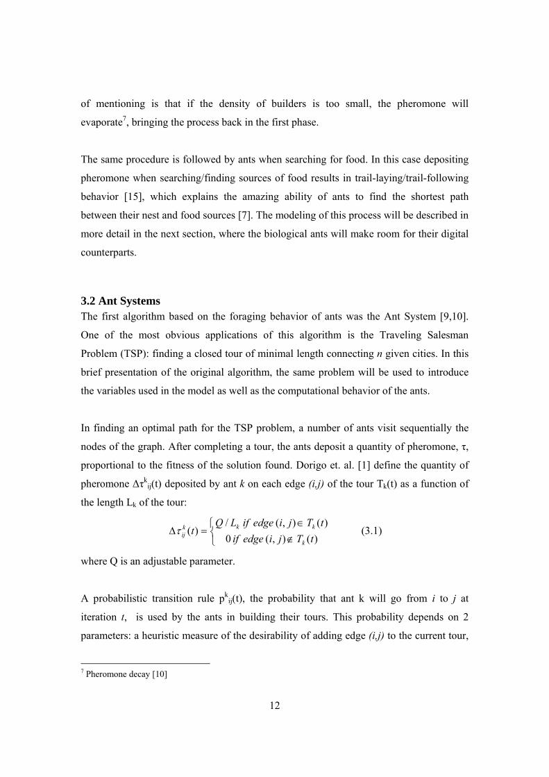
In finding an optimal path for the TSP problem, a number of ants visit sequentially the
nodes of the graph. After completing a tour, the ants deposit a quantity of pheromone, τ,
proportional to the fitness of the solution found. Dorigo et. al. [1] define the quantity of
pheromone Δτkij(t) deposited by ant k on each edge (i,j) of the tour Tk(t) as a function of
the length Lk of the tour:
⎩⎨⎧
∉∈
=Δ)(),(0
)(),(/)(
tTjiedgeiftTjiedgeifLQ
tk
kkkijτ (3.1)
where Q is an adjustable parameter.
A probabilistic transition rule pkij(t), the probability that ant k will go from i to j at
iteration t, is used by the ants in building their tours. This probability depends on 2
parameters: a heuristic measure of the desirability of adding edge (i,j) to the current tour,
7 Pheromone decay [10]
13
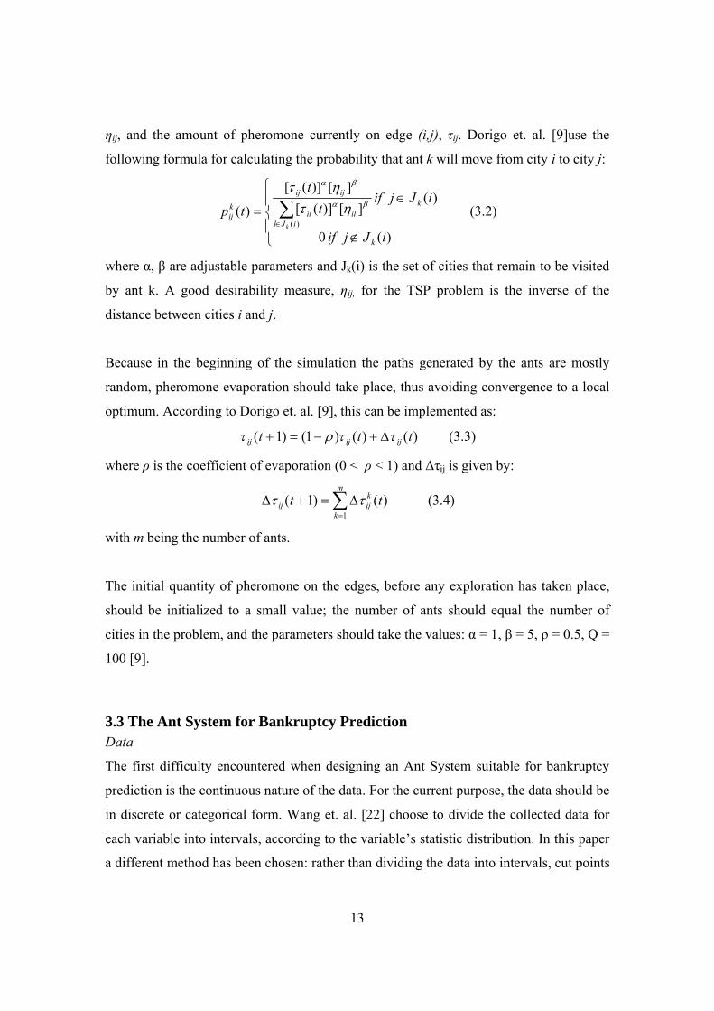
ηij, and the amount of pheromone currently on edge (i,j), τij. Dorigo et. al. [9]use the
following formula for calculating the probability that ant k will move from city i to city j:
⎪⎩
⎪⎨
⎧
∉
∈= ∑
∈
)(0
)(][)]([
][)]([
)()(
iJjif
iJjift
t
tp
k
k
iJlilil
ijij
kij
k
βα
βα
ητητ
(3.2)
where α, β are adjustable parameters and Jk(i) is the set of cities that remain to be visited
by ant k. A good desirability measure, ηij, for the TSP problem is the inverse of the
distance between cities i and j.
Because in the beginning of the simulation the paths generated by the ants are mostly
random, pheromone evaporation should take place, thus avoiding convergence to a local
optimum. According to Dorigo et. al. [9], this can be implemented as:
)()()1()1( ttt ijijij ττρτ Δ+−=+ (3.3)
where ρ is the coefficient of evaporation (0 < ρ < 1) and Δτij is given by:
∑=
Δ=+Δm
k
kijij tt
1
)()1( ττ (3.4)
with m being the number of ants.
The initial quantity of pheromone on the edges, before any exploration has taken place,
should be initialized to a small value; the number of ants should equal the number of
cities in the problem, and the parameters should take the values: α = 1, β = 5, ρ = 0.5, Q =
100 [9].
3.3 The Ant System for Bankruptcy Prediction Data
The first difficulty encountered when designing an Ant System suitable for bankruptcy
prediction is the continuous nature of the data. For the current purpose, the data should be
in discrete or categorical form. Wang et. al. [22] choose to divide the collected data for
each variable into intervals, according to the variable’s statistic distribution. In this paper
a different method has been chosen: rather than dividing the data into intervals, cut points

14
are generated based on the statistics of each of the variables in the analysis. This way the
original data stays intact, while the ants operate on a graph composed of the generated
cut-points for each of the variables. All possible cut-points for ratio Xn are obtained by
dividing the interval [minxn, maxxn] in smaller intervals of size SXn, where minxn and maxxn
represent the smallest value and respectively the largest value of ratio Xn encountered in
the data set and SXn represents the distance between 2 consecutive cut-points for ratio Xn.
The values obtained in this manner represent the vector of all acceptable cut-points for
ratio Xn.
Classification Rule Having the data defined as cut-points rather than continuous values, a classification rule
is defined as R = {Cx1, Cx2, Cx3, Cx4, Cx5}, where Cxn represents the cut-point value of
ratio Xn for which the fitness function is maximized. A firm with values smaller or equal
to R for each financial ratio is predicted to go bankrupt, otherwise not. For example, a
firm Fk is considered to go bankrupt if, for all its characteristic ratios Xki, the following
relationship holds: { }5,4,3,2,1, ∈≤ iCX xiki ; if at least one of the inequalities is false, the
firm will be classified as not bankrupt.
Fitness Function The goal of this simulation is to find a classification rule that will be able to make a good
separation between bankrupt and non-bankrupt firms, based on the five financial ratios.
Taking this goal into account, the fitness value FITRk of a classification rule Rk is defined
as: ++ += RkRkRk NBBFIT (3.5)
where BRk+ is the number of bankrupt firms correctly predicted by the classification rule
Rk and NBRk+ is the number of non-bankrupt firms correctly predicted by the same rule.
In other words, the fitness value FITRk of a classification rule Rk is equal to the total
number of correctly classified firms, bankrupt and non-bankrupt. For reasons that will
become clear in the rest of this chapter, the fitness value is not expressed as a percentage
(thus dividing by the total number of firms in the dataset).

15
During each iteration, each ant constructs its solution by choosing one cut-point for each
financial ratio based on the two parameters τij (pheromone) and ηij (distance).
Pheromone Following the example of the more sophisticated mechanisms evolved by some species of
ants [9,14], the amount of pheromone deposited on the edges composing the solution
should be proportional to the fitness of that solution. For the current problem, the amount
of pheromone deposited by the ants on each edge belonging to a solution is equal to the
fitness value of that solution, FITRk, as calculated by formula (3.5).
Distance Unlike in the TSP problem, there is no physical distance between the nodes (cut-points)
of the graph. A distance measure should however be used since, according to Dorigo et.
al. [9], only taking the amount of pheromone into account will lead to a stagnation
situation (all ants generate the same, sub-optimal tour). The distance measure for the
bankruptcy problem should replicate the purpose of distance in the TSP problem, but this
time taking into account a different fitness function, see 3.5. Since this fitness function
represents the predictive power of all 5 ratios, it seems like a good idea to calculate the
distance between two cut-points belonging to different ratios as the predictive power of
those two points on the original dataset. For the current purpose, the distance DCim,Cjn
between cut-point m belonging to ratio Xi and cut-point n belonging to ration Xj is
defined as: ++ += CjnCimCjnCimCjnCim NBBD ,,, (3.6)
where BCim,Cjn+ represents the number of bankrupt firms correctly predicted by only using
the two cut-points Cim and Cjn, NBCim,Cjn+ represents the number of non-bankrupt firms
correctly predicted by the same two cut-points, Cim and Cjn represent cut-points m, n
belonging to ratio Xi, Xj.

16
Probabilistic Transition Rule Due to the different nature of the current problem, the probabilistic transition rule by
which ants choose the next point on their path must also be slightly modified. In this case,
the term [τij]α[ηij] β is not divided by the total pheromone and distance of all points in the
graph, but only by the total pheromone and distance for all cut-points belonging to a ratio
Xi. Expression (3.2) becomes:
∑∈
=
)(
)]([)]([)]([)]([
)(
iVlilil
ijijij
k
tttt
tp βα
βα
ητητ
(3.7)
where τ is the pheromone trail, η is the distance and α, β are adjustable parameters. In this
case, the set Vk(i) containing all the cities that ant k can visit when in city i represents all
the cut-points of ratio Xn from which the ant can choose in building its solution.
The Algorithm In searching for the best classification rule, the ants employ the following procedure: in
each iteration i, each ant j chooses the next cut-point to add to its solution based on the
probabilistic rule given by (3.7). A cut-point is chosen for each ratio, in the following
order: Cx1 Cx2 Cx3 Cx4 Cx5. Having completed a tour, the fitness value of each
of the solutions generated by the j ants during iteration i is calculated according to
expression (3.5). At the end of each iteration the pheromone trails are updated based on
the fitness values of the solutions, as illustrated in expression (3.3), taking pheromone
decay (ρ) into account. The simulation continues until a previously set percentage of ants
have converged to the same solution. Following the reasoning of Dorigo et. al. [1], the
number of ants is chosen according to the total number of cut-points, and the parameter
values are set to: α = 1, β = 5, ρ = 0.5. The pseudo code of the Ant System for bankruptcy
prediction is rendered below:
procedure AS initialize pheromone trails calculate distances
while end condition not satisfied do move all ants based on pij update pheromone trails
end while end AS

17
4. Experimental Setup In total, 4 types of experiments have been run. The first type, altman_all, uses the entire
altman_1Y dataset in order to find the best classification rule by which the dataset can be
divided into bankrupt and non-bankrupt firms. The same procedure is followed in the
second type of experiments, 110_all, this time making use of the entire 110_2Y dataset.
The third and fourth type of experiments (altman_div and 110_div) make use of the
training and test sets derived from altman_1Y and 110_2Y, respectively.
In all four experiments, the performance of the Ant System is compared to the
performance of Discriminant Analysis on the same data. Due to the random search
characteristics of the Ant System, this algorithm is ran ten times for each experiment.
Results are gathered from all ten runs in order to provide average information on the
performance of the Ant System.
In the remaining part of this chapter, the parameters used in the experiments are
presented. For each type of experiment values will be provided for: α, β (the adjustable
parameters), ρ (pheromone decay), m (number of ants), SXn (the vector containing the
distance between two consecutive cut-points for each of the five financial ratios), EC (the
end condition used in the experiment, represented as the percentage of ants that must
converge to the same solution before stopping the simulation).
Experiment 1 & 3: altman_all, altman_div
For these two experiments, the values chosen for the parameters α, β and ρ are the same
values used by Dorigo et. al. [9]. The number of ants (m) and the distances between two
consecutive cut-points for each financial ratios have been determined after running a
number of experiments and inspecting the statistic properties of the datasets. The values
are summarized below:
α = 1, β = 5, ρ = 0.5, m = 40
SXn = [3, 3, 3, 10, 0.1]
EC = 80%

18
Experiment 2 & 4: 110_all, 110_div
For these two experiments, the values chosen for the parameters α, β and ρ are again
identical to the values used by Dorigo et. al. [9]. The number of ants (m) and the
distances between two consecutive cut-points for each financial ratios are again
determined after carefully inspecting the statistic properties of the datasets and through
computational experiments. The values are summarized below:
α = 1, β = 5, ρ = 0.5, m = 30
SXn = [0.05, 0.05, 0.05, 10, 0.1]
EC = 80%
The fact that the two SXn vectors present different values for the first three financial ratios
is due to the differences in the data scaling employed on the two datasets. While the data
in the 110_2Y dataset has been left intact (no scaling occurred), the data on the first three
financial ratios in the altman_1Y dataset was probably multiplied by 10, most likely for
symmetry reasons. This should not affect the performance of the algorithm, since this
scaling is indirectly contained into the SXn vectors. The lower number of ants used in the
experiments on the 110_2Y dataset is due to the smaller number of cut-points generated
from this dataset. This is in concordance with the reasoning of Dorigo et. al. [9] that the
number of ants should be equal to the number of sites in the TSP problem. For the current
purpose, better results have been achieved with a number of ants smaller than the total
number of cut-points defining the search space, most likely because of the different
nature of this space when compared to the TSP graph. Even though not equal to the
number of cut-points, the number of ants is however proportional to the number of sites
in the bankruptcy prediction problem.

19
5. Results In this chapter, the results obtained by using both the Ant System (AS) and Discriminant
Analysis (DA) on the four datasets are presented. For each experiment, data from 10
consecutive runs is gathered for the AS and the results are presented as average values. In
the case of DA, the results represent values obtained after one run8. The variables
considered relevant are: type 1 err. (number of bankrupt companies classified as non-
bankrupt), type 2 err. (number of non-bankrupt companies classified as bankrupt), hitrate
(number of companies, bankrupt and non-bankrupt, correctly classified), st. dev.
(standard deviation of best solution; only for AS), min. (smallest hitrate; only for AS) and
max. (highest hitrate; only for AS). A more detailed overview of the results can be found
in Appendix B of this paper.
5.1 Experiment 1: altman_all The dataset used in this experiment is the entire altman_1Y dataset. The AS is ran ten
times, using the same parameter values for all ten runs. The average values are then
compared to the results obtained after running DA once on the same dataset. The results
are presented in table 5.1:
type 1 err. type 2 err. hitrate st. dev. min. max. AS 2.8 (8.5%) 1.6 (4.8%) 93.3% 1.06 92.4% 95.5% DA 2 (6.1%) 1 (3.0%) 95.5% N/A N/A N/A
Table 5.1: altman_all results
Even though there is a difference between the average hitrate of the AS and the hitrate
achieved by DA, this difference is small. The AS performs slightly worse on the dataset,
achieving a hitrate that is 2.2% lower than the DA hitrate. This difference in hitrates is
roughly equivalent to one extra firm misclassified by the AS. Even though, in one of the
runs, the AS equaled the hitrate of DA on the altman_1Y dataset, the average hitrate is
93.3%; this is mainly due to the fact that the most common hitrates obtained in the ten
8 Different runs of discriminant analysis on the same data, using the same parameters, provide identical results. For this reason, one run is considered sufficient.
20
runs are 93.9% and 92.4%, respectively. When comparing the two hitrates, it should be
noted that the altman_1Y dataset is the same dataset that was used to select the five
financial ratios used in this study. The relatively small standard deviation of the hitrates
obtained by using AS leads to the conclusion that the algorithm performs relatively stable
on this dataset.
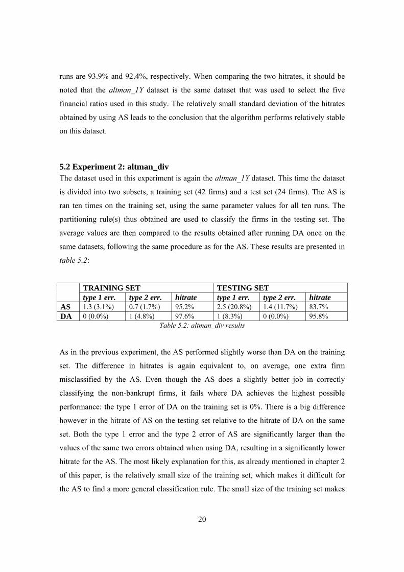
5.2 Experiment 2: altman_div The dataset used in this experiment is again the altman_1Y dataset. This time the dataset
is divided into two subsets, a training set (42 firms) and a test set (24 firms). The AS is
ran ten times on the training set, using the same parameter values for all ten runs. The
partitioning rule(s) thus obtained are used to classify the firms in the testing set. The
average values are then compared to the results obtained after running DA once on the
same datasets, following the same procedure as for the AS. These results are presented in
table 5.2:
TRAINING SET TESTING SET type 1 err. type 2 err. hitrate type 1 err. type 2 err. hitrate
AS 1.3 (3.1%) 0.7 (1.7%) 95.2% 2.5 (20.8%) 1.4 (11.7%) 83.7% DA 0 (0.0%) 1 (4.8%) 97.6% 1 (8.3%) 0 (0.0%) 95.8%
Table 5.2: altman_div results
As in the previous experiment, the AS performed slightly worse than DA on the training
set. The difference in hitrates is again equivalent to, on average, one extra firm
misclassified by the AS. Even though the AS does a slightly better job in correctly
classifying the non-bankrupt firms, it fails where DA achieves the highest possible
performance: the type 1 error of DA on the training set is 0%. There is a big difference
however in the hitrate of AS on the testing set relative to the hitrate of DA on the same
set. Both the type 1 error and the type 2 error of AS are significantly larger than the
values of the same two errors obtained when using DA, resulting in a significantly lower
hitrate for the AS. The most likely explanation for this, as already mentioned in chapter 2
of this paper, is the relatively small size of the training set, which makes it difficult for
the AS to find a more general classification rule. The small size of the training set makes
21
it more likely that the AS will overfit the data, finding a rule that is too specific and that
will not perform well on ‘unseen’ datasets. Sustaining this affirmation is the fact that the
AS performed better on a larger dataset, consisting of 110 firms; on this dataset it
outperformed DA, as it will be shown in the following two experiments.
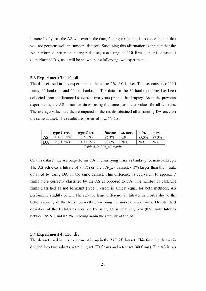
5.3 Experiment 3: 110_all The dataset used in this experiment is the entire 110_2Y dataset. This set consists of 110
firms, 55 bankrupt and 55 not bankrupt. The data for the 55 bankrupt firms has been
collected from the financial statement two years prior to bankruptcy. As in the previous
experiments, the AS is ran ten times, using the same parameter values for all ten runs.
The average values are then compared to the results obtained after running DA once on
the same dataset. The results are presented in table 5.3:
type 1 err. type 2 err. hitrate st. dev. min. max. AS 11.4 (20.7%) 3.7(6.7%) 86.3% 0.9 85.5% 87.3% DA 12 (21.8%) 10 (18.2%) 80.0% N/A N/A N/A
Table 5.3: 110_all results
On this dataset, the AS outperforms DA in classifying firms as bankrupt or non-bankrupt.
The AS achieves a hitrate of 86.3% on the 110_2Y dataset, 6.3% larger than the hitrate
obtained by using DA on the same dataset. This difference is equivalent to approx. 7
firms more correctly classified by the AS as opposed to DA. The number of bankrupt
firms classified as not bankrupt (type 1 error) is almost equal for both methods, AS
performing slightly better. The relative large difference in hitrates is mostly due to the
better capacity of the AS in correctly classifying the non-bankrupt firms. The standard
deviation of the 10 hitrates obtained by using AS is relatively low (0.9), with hitrates
between 85.5% and 87.3%, proving again the stability of the AS.
5.4 Experiment 4: 110_div The dataset used in this experiment is again the 110_2Y dataset. This time the dataset is
divided into two subsets, a training set (70 firms) and a test set (40 firms). The AS is ran

22
ten times on the training set, using the same parameter values for all ten runs. The
partitioning rule(s) thus obtained are used to classify the firms in the testing set. The
average values are then compared to the results obtained after running DA once on the
same datasets, following the same procedure as for the AS. These results are presented in
table 5.4:
TRAINING SET TESTING SET type 1 err. type 2 err. hitrate type 1 err. type 2 err. hitrate
AS 6.1 (17.4%) 3.1 (8.9%) 86.9% 4.0 (20.0%) 3.9 (19.5%) 80.5% DA 6 (17.1%) 10 (28.7%) 77.1% 6 (30.0%) 6 (30.0%) 70.0%
Table 5.4: 110_div results
Again, the AS performs better than DA on both the training set as well as on the testing
set. The DA is outperformed by 9.8% on the training set, and this difference increases
even more, to 10.5% (equivalent to approx. 4 firms less that the AS misclassifies when
compared to DA) on the test set. The difference between the hitrate on the training set
and the hitrate on the testing set is 6.4% for the AS and 7.1% for DA. Even though not by
much, it can be concluded that the AS performed better in generalizing when compared
to DA, this time not overfitting the (larger) training set. The difference of 9.8% between
the hitrates of the two algorithms on the training set is mostly due to the better capacity of
the AS in correctly classifying the non-bankrupt firms. The type 2 error on the training
set drops from 28.7% (equivalent to 10 firms) for DA to only 8.9% (equivalent to 3
firms) for AS, while the type 1 error stays more or less constant around the value of 6.

23
6. Discussion In this chapter, the results obtained by using the slightly modified Ant System for
bankruptcy prediction are discussed, together with the modifications made to the original
algorithm. This chapter provides the reader with a discussion on three aspects:
classification accuracy, external validity and computational efficiency.
6.1 Classification Accuracy and External Validity The AS did a good job overall in separating the bankrupt from the non-bankrupt firms in
the two datasets. Even though slightly outperformed by DA on the altman_1Y dataset, the
AS was capable of better performance on the 110_2Y dataset. The classification error of
AS on the entire altman_1Y dataset, larger than the error of DA on the same dataset by
one firm, is consider acceptable. A very important aspect that should be taken into
account when making this comparison is the fact that the altman_1Y is the same set used
by Altman in [1] for selecting the five financial ratios that are also used in this study.
Even then, the AS is able to equal the hitrate of DA on this dataset, but not in each of the
ten runs, and for this reason the average hitrate obtained when classifying the data by
means of the AS is slightly lower. As one would expect, this scenario repeats itself on the
alman_1Y_train dataset, the dataset containing only 42 out of the 66 corporations listed
in the original set. The AS is able to correctly classify 95.2 of the firms, a slightly lower
value than the hitrate of 97.6% of DA on the same dataset. Again, the difference between
the hitrates is equivalent to 1 firm. A large difference in hitrates is encountered when
testing the ability to generalize (using the altman_1Y_train dataset) of both algorithms on
the altman_1Y_test dataset. Due to the relatively small size of the training dataset, the AS
is not able to derive a more general classification rule, which results in a difference of
12.1% in favor of DA when comparing the two hitrates. The algorithm was also tested on
a larger dataset, 110_2Y, containing data on 110 firms. This time, the AS outperformed
DA both on the entire dataset as well as on the training and test sets. The AS showed a
good ability to generalize from a larger training set (70 firms), outperforming DA on both
the training and the testing set. The AS proved better in classifying the firms in the whole
110_2Y dataset, outperforming DA by 6.3%, which is roughly equivalent to seven firms.

24
The AS was able to generalize slightly better from the data in the training set, in the end
outperforming DA by an average of 10.5% on the testing set, roughly equivalent to 4
firms. Another aspect worth of mentioning is the fact that, even though the AS does not
converge to an identical solution in all ten runs for each of the four experiments, the
standard deviation of the ten hitrates obtained by AS after 10 runs is relatively small,
proving a good ability of the algorithm to provide similar (and often identical) solutions
during different runs, on the same dataset, by using the same parameters.
6.2 Computational Efficiency One of the features making the Ant System very attractive for optimum-seeking problems
is its simplicity. With very little knowledge on the data or nature of the problem, the
virtual ants are able to find their (fitness maximizing) way in a semi-chaotic and often
complex space. Redefining bankruptcy prediction as a search for optimal cut-points in the
space defined by the five financial ratios reduces this space, making it more or less
independent of the size of the dataset. The 15 minutes that it takes the ‘modified ants
algorithm’ (MAA) developed by Wang et. al. [22] to find a satisfactory solution are
brought down to 5-7 minutes by the Ant System presented in this paper. It should be
taken into account however that the search space used by the MAA differs from the one
used for the current purpose.

25
7. Conclusion and further research
Using the lessons provided by what David Rogers [21] calls ‘the most extensive
computation known [that] has been conducted over the last billion years on a planet-wide
scale’, this study is based on imitating a small part of the evolution of life with the
purpose of applying it on a big problem: corporate bankruptcy. By modeling the behavior
of ants it is possible to achieve good results in solving problems that at a first sight seem
so different than the problems encountered by ants in their actual environment. A few
abstractions are, of course, necessary, as well as the adaptation of both the ants and the
bankruptcy ‘environment’. Having done this, imitating evolution proves (again) to be a
lucrative business, even when business failure is the subject being investigated.
The Ant System that has been used in this paper is based on a number of parameters,
problem-specific, which the author has determined through different computational
experiments. A more inspired way of doing this would be to evolve different ant types
(species), where the particularities of each species are given by the values of its
parameters. Parameters such as pheromone decay and the number of ants searching for a
solution could be evolved towards optimal values, maybe further improving the results
obtained by the Ant System. Unfortunately, this subject seemed too large to be
investigated for the purpose of this study, but interesting for further research.

26
Bibliography
[1] Altman, E.I.: Financial Ratios, Discriminant Analysis and the Prediction of
Corporate Bankruptcy , Journal of Finance, 23, 1968, 589-609.
[2] Altman E.I., Hadelman R.G., Narayanan P: Zeta Analysis, a New Model to
Identify Bankruptcy Risk of Corporations, Journal of Banking and Finance, 1,
1977, 29-51.
[3] Altman E.I., Avery R., Eisenbeis R., Stinkey J.: Application of Classification
Techniques in Business, Banking and Finance, Contemporary Studies in
Economic and Financial Analysis, Vol. 3, 1981, JAI Press.
[4] Aguilar J., Velasquez L., Velasquez M.E.: The Combinatorial Ant System,
Applied Artificial Intelligence, 18, 2004, 427-446.
[5] Carroll C.R., Janzen D.H.: Ecology of Foraging by Ants, Annual Review of
Ecology and Systematics, Vol. 4, 1973, 231-257.
[6] Dambolena I. G., Sarkis J. K.: Ration Stability and Corporate Failure, The Journal
of Finance, Vol. 35, No. 4, September 1980, 1017-1026.
[7] Deneubourg J.-L., Aron S., Goss S., Pasteels J.-M.: The self-organizing
exploratory pattern of the Argentine ant, Journal of Insect Behavior., 3, 1990,
159-168.
[8] Dorigo M., Colorni A., Maniezzo V.: Positive Feedback as a Search Strategy, T
echnical Report TR91-016, 1991, Politecnico di Milano.
[9] Dorigo M., Bonabeau E., Theraulaz G.: Ant Algorithms and Stigmergy, Future
Generation Computer Systems, 16, 2000, p. 851-871.
27
[10] Dorigo M., di Caro G.: The ant colony optimization meta-heuristic, in: D. Come,
M. Dorigo, F. Glover (Eds.), New Ideas in Optimization, McGraw-Hill, London,
UK, 1999, p. 11-32.
[11] Dorigo M., di Caro G., Gambardella L.M.: Ant algorithms for discrete
optimization, Artificial Life 5 (2), 1999, 137-172.
[12] Dorigo M., Gambardella L.M.: Ant colonies for the traveling salesman problem,
Biosystems 43, 1997, 73-81.
[13] Grassé P.P.: La reconstruction du nid et les coordinations interindividuelles chez
bellicositermes natalensis et cubitermes sp. La théorie de la stigmergie: essai
d’interprétation du comportement des termites constructeurs, Insectes Sociaux 6,
1959, 41-81.
[14] Hangartner, W.: Trail-Laying in the Subterranean Ant Acanthomyops interjectus,
Journal of Insect Physiology, XV, 1969, 1-4.
[15] Hőlldobler B., Wilson E.O.: The Ants, Springer, Berlin, 1990.
[16] Kirman A.: Ants, Rationality, and Recruitment, The Quarterly Journal of
Economics, Vol. 108, No. 1, 1993, 137-156.
[17] LoPucki L.M., Doherty J.W.: The Determinants of Professional Fees in Large
Bankruptcy Reorganization Cases, Journal of Empirical Legal Studies, Vol. 1,
Issue 1, March 2004, 111-141.
[18] Middendorf M., Reischle F., Schmeck H.: Multi Colony Ant Algorithms, Journal
of Heuristics, 8, 2002, 305-320.

28
[19] Monmarché N., Venturini G., Slimane M.: On How Pachycondyla apicalis Ants
Suggest a New Search Algorithm, Future Generation Computer Systems, 16,
2000, 937-946.
[20] Rajendran C., Ziegler H.: Two Ant-colony Algorithms For Minimizing Total
Flowtime In Permutation Flowshops, Computers & Industrial Engineering, 48,
2005, 789-797.
[21] Rogers, D.: Weather Prediction Using a Genetic Memory, Research Institute for
Advance Computer Science (RIACS) Technical Report 90.6, February 1990.
[22] Wang C., Zhao X., Kang L.S: Bussiness failure prediction using modified ants
algorithm,
[23] Zne-Jung L., Chou-Yuan L.: A Hybrid Search Algorithm With Heuristics For
Resource Allocation Problem, Information Sciences, 173, 2005, 155-167.
29
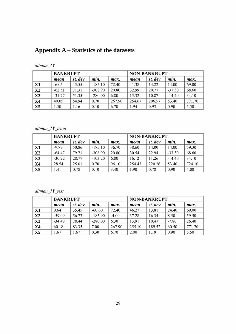
Appendix A – Statistics of the datasets
altman_1Y
BANKRUPT NON-BANKRUPT mean st. dev min. max. mean st. dev min. max. X1 -6.05 45.55 -185.10 72.40 41.38 14.22 14.00 69.00 X2 -62.51 71.31 -308.90 20.80 32.99 20.77 -37.30 68.60 X3 -31.77 51.35 -280.00 6.80 15.32 10.87 -14.40 34.10 X4 40.05 54.94 0.70 267.90 254.67 206.57 53.40 771.70 X5 1.50 1.16 0.10 6.70 1.94 0.93 0.90 5.50
altman_1Y_train
BANKRUPT NON-BANKRUPT mean st. dev min. max. mean st. dev min. max. X1 -9.87 50.86 -185.10 36.70 38.60 14.00 14.00 59.30 X2 -64.47 79.71 -308.90 20.80 30.54 22.94 -37.30 68.60 X3 -30.22 28.77 -103.20 6.80 16.12 11.26 -14.40 34.10 X4 28.54 25.01 0.70 96.10 254.43 220.26 53.40 724.10 X5 1.41 0.78 0.10 3.40 1.90 0.78 0.90 4.00
altman_1Y_test
BANKRUPT NON-BANKRUPT mean st. dev min. max. mean st. dev min. max. X1 0.64 35.45 -60.60 72.40 46.27 13.81 24.40 69.00 X2 -59.09 56.77 -185.90 -4.00 37.28 16.34 8.50 59.50 X3 -34.48 78.44 -280.00 6.30 13.91 10.47 -7.80 26.40 X4 60.18 83.35 7.00 267.90 255.10 189.52 60.50 771.70 X5 1.67 1.67 0.30 6.70 2.00 1.19 0.90 5.50

30
Appendix A - continued
110_2Y
BANKRUPT NON-BANKRUPT mean st. dev min. max. mean st. dev min. max. X1 0.12 0.20 -0.42 0.55 0.31 0.16 -0.15 0.75 X2 -0.14 0.41 -1.27 0.46 0.21 0.29 -0.67 0.79 X3 -0.10 0.35 -2.38 0.14 0.12 0.10 -0.03 0.54 X4 0.79 1.53 0.00 9.92 33.66 72.23 0.25 427.90 X5 1.15 0.54 0.46 3.16 1.20 0.46 0.30 2.41
110_2Y_train
BANKRUPT NON-BANKRUPT mean st. dev min. max. mean st. dev min. max. X1 0.14 0.16 -0.36 0.55 0.30 0.17 -0.15 0.76 X2 -0.08 0.39 -1.27 0.38 0.22 0.33 -0.67 0.79 X3 -0.19 0.41 -2.38 0.11 0.13 0.10 -0.03 0.43 X4 0.73 1.05 0.00 5.04 43.49 82.93 0.25 427.90 X5 1.11 0.53 0.47 3.16 1.23 0.41 0.59 2.24
110_2Y_test
BANKRUPT NON-BANKRUPT mean st. dev min. max. mean st. dev min. max. X1 0.08 0.25 -0.42 0.38 0.35 0.16 0.12 0.66 X2 -0.25 0.46 -1.25 0.47 0.18 0.20 -0.38 0.47 X3 -0.12 0.23 -0.61 0.14 0.11 0.11 0.01 0.54 X4 0.91 2.20 0.00 9.92 16.45 45.08 0.73 206.08 X5 1.23 0.57 0.46 2.90 1.13 0.54 0.30 2.41

31
Appendix B – Detailed results of the four experiments
altman_all altman_div (train) altman_div (test) R1 93.9 95.2 83.3 R2 92.4 95.2 87.5 R3 92.4 95.2 87.5 R4 93.9 95.2 83.3 R5 95.5 95.2 83.3 R6 92.4 95.2 79.2 R7 93.9 95.2 83.3 R8 93.9 95.2 83.3 R9 92.4 95.2 83.3 R10 92.4 95.2 83.3 mean 93.3 95.2 83.7 st. dev. 1.1 0.0 2.4 min. 92.4 95.2 79.2 max. 95.5 95.2 87.5
Hitrates of AS on the altman_1Y, altman_1Y_train and altman_1Y_test datasets, expressed as percentage for each run.
altman_all altman_div (train) altman_div (test) type 1 type 2 type 1 type 2 type 1 type 2 R1 2 1 2 0 3 1 R2 3 2 1 1 3 0 R3 4 2 1 1 2 1 R4 4 0 2 0 3 1 R5 1 2 1 1 2 2 R6 3 2 2 0 4 1 R7 2 2 1 1 2 2 R8 4 0 1 1 2 2 R9 2 3 1 1 2 2 R10 3 2 1 1 2 2 mean 2.8 1.6 1.3 0.7 2.5 1.4 st. dev. 1.06 0.97 0.48 0.48 0.71 0.70 min. 1 0 1 0 2 0 max. 4 3 2 1 4 2
Type 1 and type 2 errors on the altman_1Y, altman_1Y_train and altman_1Y_test datasets, expressed as absolute values for each run.

32
Appendix B - continued
110_all 110_div (train) 110_div (test) R1 87.3 87.1 77.5 R2 85.5 87.1 77.5 R3 87.3 85.7 80.0 R4 85.5 87.1 85.0 R5 85.5 87.1 80.0 R6 85.5 87.1 82.5 R7 87.3 85.7 82.5 R8 85.5 87.1 77.5 R9 86.4 87.1 82.5 R10 87.3 87.1 80.0 mean 86.3 86.9 80.5 st. dev. 0.9 0.6 2.6 min. 85.5 85.7 77.5 max. 87.3 87.1 85.0 Hitrates of AS on the 110_1Y, 110_1Y_train and 110_1Y_test datasets,
expressed as percentage for each run.
110_all 110_div (train) 110_div (test) type 1 type 2 type 1 type 2 type 1 type 2 R1 11 3 7 2 6 3 R2 13 3 5 4 3 6 R3 11 3 7 3 5 3 R4 10 6 6 3 3 3 R5 13 3 5 4 2 6 R6 11 5 6 3 4 3 R7 11 3 7 3 4 3 R8 11 5 5 4 4 6 R9 12 3 6 3 4 3 R10 11 3 7 2 5 3 mean 11.4 3.7 6.1 3.1 4 3.9 st. dev. 0.97 1.16 0.88 0.74 1.15 1.45 min. 10 3 5 2 2 3 max. 13 6 7 4 6 6
Type 1 and type 2 errors on the 110_1Y, 110_1Y_train and 110_1Y_test datasets, expressed as absolute values for each run.