An analysis of the effect of the growth of the informal ...

An analysis of the effect of the growth of the informal sector on tax revenue

performance in Kenya

By:

Kago Bernard Muchiri

A Research Paper submitted to the School of Economics in Partial Fulfillment of the

Requirements for the Award of the Degree of Master of Arts in Economics of the University of

Nairobi

October 2014

i

DECLARATION

This Research Paper is my original work and has not been presented for a degree in any otheruniversity.

Signed_____________________________ Date_______________________

Bernard Muchiri Kago

Admission No. X50/72721/2009

This Research Paper has been submitted for examination with our approval as Universitysupervisors.

Signed_______________________________ Date_______________________

Dr. Moses K. Muriithi

Signed_______________________________ Date_______________________

Dr. Urbanus Kioko

ii

DEDICATION

This research paper is dedicated to my late teacher, Mrs. Mary Mwihaki Ngigi. May her soul restin peace.

iii

ACKNOWLEDGEMENTS

I wish to acknowledge the debt of gratitude that I owe to the people who have made it possible to

bring this research paper to fruition. First of all I wish to thank my first supervisor, Dr. Muriithi

for his erstwhile guidance and mentorship during the period of research as well as my second

supervisor Dr. Kioko for his unfailing support. I also wish to appreciate the invaluable critique of

my other teachers and colleagues during and after the discussion of my research proposal during

the presentation seminar.

I cannot forget to thank my parents, Mr and Mrs. Kago for supporting me throughout my years

of education, as well as for their wisdom and affection. At the same time, I would like to thank

my wife Carol for her patience, support and encouragement, as well as my sons Austin and

Adrian for understanding my moments of solitude in the course of the research.

Special mention goes to my friend and brilliant student of economics, Mr. Bosco Okumu, who

assisted in reviewing literature and analyzing data for this paper. I would not fail to appreciate

the encouragement I received from my brothers and sisters, who always offered moral support.

This is especially so for my brother, Gerald Njihia who accompanied me to the proposal defence

session, and stayed patiently to the end. I also thank my superiors and colleagues at Kenya

Revenue Authority for granting me leave whenever I would need to work on data collection and

analysis for the research project.

Last, but most importantly, I thank Almighty God for giving me the opportunity and strength to

accomplish this work. Finally, I acknowledge responsibility for all errors, omissions and views

expressed in this paper.

iv

ABSTRACT

Despite far reaching reforms implemented in taxation in Kenya, tax revenue collection has not

yet reached a level where it can meet all the expenditure requirements of the government. This is

more so the case during this crucial transitional period to the new constitutional dispensation

where the coming into place of a devolved government structure means the public sector wage

bill has been increasing drastically. One of the possible strategies to increase tax revenue

collection is to expand the tax base by bringing in more businesses into the tax bracket. Most of

these untaxed businesses are in the informal sector, and therefore there is a need to analyze this

expansive sector and how it impacts on the overall revenue performance. This is the problem

tackled by this paper. The key objective of the study was to determine the impact of the growth

of the informal sector on tax revenues, with the aim of coming up with policy recommendations

on the way forward regarding the taxation of the informal sector. Using statistical methodology,

the study sought to formulate a model based on the existing data on taxation and the informal

sector, as well as other variables that were identified as determinants of tax revenue based on

past studies. The study employed time series data from secondary sources, including past

research papers, Kenya Economic Surveys, World Bank and IMF Publications, Working papers,

Journals, web sources and text books. The empirical analysis used the Ordinary Least Squares

regression method with the accompanying statistical tests. The results showed that an increase in

the size of the informal sector leads to a decrease in revenue performance and vice versa, and is

statistically significant. The results also indicated that FDI, openness to trade, and per capita

GDP are compellingly significant in determining tax revenue performance. The key policy

recommendations indicate a need to formulate policies that are aimed at including the informal

sector in the tax bracket by fostering voluntary compliance and reducing costs of tax collection.

v

ACRONYMS AND ABBREVIATIONS

AERC African Economic Research Consortium

AGDP Agriculture Sector contribution to GDP

CPI Consumer Price Index

ECM Electricity Consumption Method

FDI Foreign Direct Investment

GDP Gross Domestic Product

GNP Gross National Product

HTT Hard To Tax

ICLS International Conference of Labour Statisticians

IFEM Inter-bank Foreign Exchange Market

ILC International Labour Conference

ILO International Labour Organization

KIPPRA Kenya Institute of Public Policy and Research

KRA Kenya Revenue Authority

MEC Modified Electricity Consumption method

MIMIC Multiple Indicators, Multiple Causes method

MPND Ministry of Planning and National Development

OLS Ordinary Least Squares method

PAYE Pay As You Earn

PIN Personal Identification Number

RER Real Exchange Rate

SME Small and Medium Enterprises

VAT Value Added Tax

vi

TABLE OF CONTENTS

DECLARATION ............................................................................................................................. i

DEDICATION................................................................................................................................ ii

ACKNOWLEDGEMENTS........................................................................................................... iii

ABSTRACT................................................................................................................................... iv

ACRONYMS AND ABBREVIATIONS....................................................................................... v

TABLE OF CONTENTS............................................................................................................... vi

LIST OF TABLES......................................................................................................................... ix

CHAPTER ONE ........................................................................................................................... 1

1.0 INTRODUCTION................................................................................................................... 1

1.1 Background ............................................................................................................................... 1

1.1.1 Historical background............................................................................................................ 1

1.1.2 Tax administration: The Kenyan scenario ............................................................................. 2

1.2 Kenya’s informal sector ............................................................................................................ 4

1.3 Problem Statement .................................................................................................................... 6

1.4 Objectives of the study.............................................................................................................. 8

1.5 Significance of the Study .......................................................................................................... 8

1.6 Justification of the study ........................................................................................................... 8

1.7 Organization of the study.......................................................................................................... 9

CHAPTER TWO ........................................................................................................................ 10

2.0 LITERATURE REVIEW .................................................................................................... 10

2.1 Introduction............................................................................................................................. 10

vii

2.2 Theoretical Literature Review ................................................................................................ 10

2.2.1 The Informal Sector ............................................................................................................. 10

2.2.2 The Dynamics underlying the growth of the Informal Sector ............................................. 12

2.2.3 The Informal Sector and Taxation ....................................................................................... 13

2.2.4 Measuring the informal sector ............................................................................................. 18

2.3 Empirical Literature Review................................................................................................... 24

2.4 Overview of the literature ....................................................................................................... 28

CHAPTER THREE .................................................................................................................... 30

3.0 METHODOLOGY ............................................................................................................... 30

3.1 Analytical Framework ............................................................................................................ 30

3.2 The Model............................................................................................................................... 31

3.2.1 Empirical model specification ............................................................................................. 31

3.2.2 Definition of Variables and a priori expectations ................................................................ 32

3.3 Stationarity, Cointegration and Diagnostic Testing................................................................ 36

3.4 Data sources ............................................................................................................................ 38

CHAPTER FOUR....................................................................................................................... 40

4.0 DATA ANALYSIS AND RESULTS ................................................................................... 40

4.1 Descriptive statistics ............................................................................................................... 40

4.2 Stationarity analysis ................................................................................................................ 41

4.3 Test for Multicollinearity........................................................................................................ 43

4.4 Autocorrelation test................................................................................................................. 44

4.5 Co-integration test................................................................................................................... 44

4.6 Discussion of the results ......................................................................................................... 48

viii

CHAPTER FIVE ........................................................................................................................ 53

5.0 CONCLUSION AND POLICY RECOMMENDATIONS ............................................... 53

5.1 Conclusion .............................................................................................................................. 53

5.2 Policy recommendations......................................................................................................... 55

REFERENCES............................................................................................................................ 60

ix

LIST OF TABLES

Table 1.1: Kenya’s revenue capacity and tax effort ....................................................................... 3

Table 3.1: Variables and expected signs....................................................................................... 35

Table 4.1: Summary statistics ....................................................................................................... 40

Table 4.2: Unit root test results..................................................................................................... 42

Table 4.3: Unit root test results after differencing........................................................................ 42

Table 4.4: Test for Multicollinearity............................................................................................. 43

Table 4.5 OLS regression results .................................................................................................. 45

Table 4.6: ADF test for residual ................................................................................................... 46

Table 4.7: Error Correction Model Results................................................................................... 47

1

CHAPTER ONE

1.0 INTRODUCTION

1.1 Background

1.1.1 Historical background

Tax policy and administration in Kenya has gone through various phases of reform over the

years. From independence in 1963 until the early 1980s, public spending in Kenya was financed

through a somewhat uncoordinated set of taxes and fees inherited from British rule and

supplemented by foreign aid inflows. The oil shock in the early 1970s led to the country’s first

significant fiscal crisis, in response to which some relatively minor tax reforms were undertaken

(Eissa et al., 2009). Sales taxes were introduced, as well as trade taxes in order to control the

increasing deficit in balance of payment. In 1986, the then government launched the tax policy

and modernization program (TMP). This program aimed at raising revenue levels by expanding

the tax base, attaining 24% tax/ GDP ratio and maintaining that level of performance, making the

tax structure more equitable and sealing tax leakage loop holes among other objectives. (Moyi

and Ronge, 2006). This target was raised to 28% in 1992. (Muriithi and Moyi, 2003). This led to

the eventual union of the various revenue departments in the Ministry of Finance under one

semi-autonomous tax agency, Kenya Revenue Authority, in 1995.

In the years immediately following the introduction of the TMP revenues gradually increased,

reaching 24.6 percent of GDP in the years 1995-96, after which they stabilized at around 23

percent until the end of the decade as recorded in the Kenya Revenue Authority’s Annual.

2

Revenue Performance Report (KRA, 2005). In 1999-2000 revenues fell below 20 percent of

GDP, and this decline continued until they reached a low of 17.8 percent of GDP in 2001-

02.(Karingi et al., 2004). Since then there has been a slow increase to slightly above 20 percent

of GDP in 2011/2012 with reforms ongoing under the Revenue Administration Reforms and

Modernization Programme (RARMP).

1.1.2 Tax administration: The Kenyan scenario

Tax revenues play a vital role in Kenya’s economic development. This can be deduced from the

attention that issues of taxation have received over the years as found in government Sessional

Papers (Republic of Kenya, 1965-2007). Tax Management Administration Guidelines (1986)

contain reforms in all areas of tax policy. They emphasize the need to raise more revenue

without increasing the burden of taxation on those who are already contributing to the exchequer.

The tax measures contained in these documents consist of broadening the tax base to include

additional sector activities and strengthen tax administration.

These measures were adopted after the government realized that the tax structure did not raise

adequate revenues thereby encouraging domestic borrowing and seeking external finance, which

constitute only temporary measures of deficit financing. Moreover, external funds could no

longer be relied on due to donor conditions and the increasing interest to channel funds to

Eastern Europe after the cold war (Gelb, 1993). Furthermore, potential sources for domestic

borrowing are few and external grants reduce autonomy and increase political and economic

dependence. The alternatives are therefore to raise money through taxation, curtail desired

government expenditures, or continuously revise the tax structure.

3

The main shortcoming of Kenya’s tax structure since independence has been its over-dependence

on a small number of sources of tax revenue, namely trade taxes, sales tax/VAT and income tax

(Ole, 1975; Muriithi and Moyi, 2003; Wawire, 2003). The trade taxes, sales tax/VAT on various

imported products are vulnerable to external events because their prices are determined in the

world market and tend to be volatile. This has resulted in inadequate tax revenues and continuous

existence of budget deficits. This also limits Kenya’s taxable capacity because tax collection

depends on the accounting veracity of formal businesses.

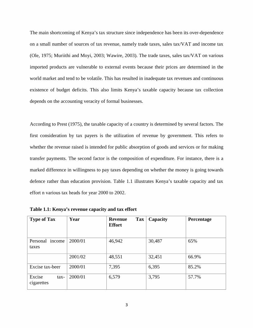
According to Prest (1975), the taxable capacity of a country is determined by several factors. The

first consideration by tax payers is the utilization of revenue by government. This refers to

whether the revenue raised is intended for public absorption of goods and services or for making

transfer payments. The second factor is the composition of expenditure. For instance, there is a

marked difference in willingness to pay taxes depending on whether the money is going towards

defence rather than education provision. Table 1.1 illustrates Kenya’s taxable capacity and tax

effort n various tax heads for year 2000 to 2002.

Table 1.1: Kenya’s revenue capacity and tax effort

Type of Tax Year Revenue TaxEffort

Capacity Percentage

Personal incometaxes

2000/01 46,942 30,487 65%

2001/02 48,551 32,451 66.9%

Excise tax-beer 2000/01 7,395 6,395 85.2%

Excise tax-cigarettes

2000/01 6,579 3,795 57.7%

4

2001/02 5,389 2,806 52.1%

Import duty 2000/01 44,651 28,664 64.2%

2001/02 43,412 21,286 49.0%

Corporate tax 2000/01 78,730 27,359 34.8%

2001/02 79,764 28,044 35.2%

VAT (Total taxbase 451,766)

2000/01 83,309 50,381 60.4%

VAT (Total taxbase 496,000)

2001/02 91,400 50,900 56%

Source: Karingi et al. (2004)

According to an evaluation study by the British Department for International Development

(DFID) of tax reforms in a number of sub-Saharan African countries, the failure to tax the

informal sector and agriculture, and the continued tendency of granting tax exemptions to

powerful businesses and individuals with close political connections provide the main reasons

why collection appears to have stagnated at a relatively low level. (DFID, 2004)

Although Kenya embarked on massive tax reforms in 1986, little is known about the

performance of the reforms in terms of raising the revenue mobilization capacity of the tax

system. This study attempts to fill this gap in knowledge.

1.2 Kenya’s informal sector

Traditionally in Kenya, informal sector activities consisted of urban artisans, but have grown to

include manufacturing, building and construction, distributive trades, transport and

communication, and community and personal services industries. Currently, the main activities

include tailoring, carpentry, blacksmithing, retail shops, groceries and kiosks, among others. The

5

sectoral distribution of these enterprises shows a wide variation, with 64.5% of the total

enterprises being in wholesale and retail trade, while only 0.3% were in private households.

Overall, 71% of industries are in the rural areas with the dominant industries being trade and

manufacturing. (Atieno, 2006)

The informal sector is a crucial sector of most of the developing countries. The liberalization and

privatization processes have resulted to the states’ failure to be the employer. The private sector

is left to take up this role. The organized private sector has been unable to absorb the growing

numbers of jobseekers, and the informal sector stepped in to fill in the gap. This indeed is the

reason why informal sector should be supported and encouraged. In most cases, the informal

sector is viewed as illegal and its activities barred by the government as well as the people

working in the formal sector. Urbanization in Kenya on the other end has been occurring in the

context of weak economic growth resulting in poor infrastructure, housing and services

especially in the slums.

The informal sector has long been an integral part of the culture and economy in Kenya. It

currently employs approximately 8.3 million people. This includes workers and

entrepreneurs/owner-managers of the enterprises. The informal sector contributes to about 18%

of the GDP. (Ogutu, 2013)

In past studies, it has been found that a significant number of citizens participating in the

informal economy do so in order to evade taxes and government regulations (Andreoni et al.,

6

1998; Feige, 1979). Increased tax revenue captured from this expansive, untapped tax base

would contribute to GDP, alleviate poverty, and improve citizens’ standard of living.

The informal sector in Kenya is characterized by:

a) Activities that are undertaken with the primary objective of self-generation of

employment and incomes mostly unregistered and unrecorded in official statistics

b) Operate in small scale and mostly have very low level of capital, productivity and income

c) Have little or no access to organized market, credit institutions, modern technology, and

formal education.

d) Many activities are carried without fixed location or in places that are not visible to the

authorities such as small shops, stalls, or home-based operations.

(Muchiri and Audi, 2007)

1.3 Problem Statement

Kenya relies heavily on tax revenue to fund government expenditure, both current and capital.

Although there has been great improvement in tax effort as a result of wide ranging reforms in

this area, revenue collection still falls short of its full potential. In the face of a ballooning annual

budget, especially with the rising wage bill occasioned by the implementation of the new

constitution, there is urgent need to re-evaluate the tax system with the aim of improving

collection. With the tax burden increasingly lying on a small section of the economy, the answer

appears to be in the unexplored revenue base, namely the informal sector.

7

Research has been carried out in the past in other countries on the revenue losses implied by the

informal sector, also referred to as the Hard to Tax sector (HTT). For the United States,

Kenadjian (1982) reports on the findings of a 1979 IRS study that estimated total unreported

taxable income of US $ 74.9 billion in 1976, of which self-employment income was US$ 33

billion; a considerable share of unreported self-employment income could be considered as

belonging to the hard-to-tax group.

According to Cheeseman and Griffiths (2006), although Kenya’s tax revenues have increased

during the recent process of reform they have fallen in relation to GDP, whilst the share of

government revenue made up through tax revenues has not increased. The question is; to what

extent does the rapid expansion of the informal sector influence tax revenue performance? In

past studies, no specific attention has been paid on the effect of the growth in the informal sector

on tax revenue collection in Kenya. This study thus aimed at filling this gap in country specific

literature on the revenue losses implied by the growth of the informal sector as well as the level

of significance.

Terkper (2003) states that developing countries lose tax revenue in proportionally greater

amounts than developed countries from the informal sector because small and medium traders

tend to thrive in underground economies, and further estimated that the tax losses could

constitute as much as 35 to 55 percent of GDP. According to a World Bank study in year 2006,

Kenya’s informal sector constituted 98 percent of all businesses in the country, absorbed

annually up to 50 per cent of new employment seekers and had an employment growth rate of

12-14 percent. (World Bank, 2006).

8

1.4 Objectives of the study

i) To determine the effect of the informal sector on tax revenue performance.

ii) To identify the other determinants of revenue performance in Kenya

iii) To draw policy implications from the above objectives.

1.5 Significance of the Study

The study contributes to the existing literature on the determinants of revenue collection in

Kenya. The results could be used to design growth-oriented programs and carry out tax changes

that are growth enhancing. The study provides an empirical groundwork on Kenya’s revenue

structures upon which prudent tax measures could be based. It identifies the effect of growth of

informal sector on revenue collection which when properly understood, documented, and

captured in relevant tax revenue models, would make it possible to estimate accurately revenues

within a specified period of time. The study also stimulates further research in the area of

taxation. The study brings together comprehensive evidence on the role the informal sector can

play in increasing revenue collection in Kenya. It provides an informed basis for taking action on

tax policy in addition to what is currently known about revenue function in Kenya.

1.6 Justification of the study

According to Eissa and Jack (2009), raising around 20 percent of GDP in taxes is either

impressive or dangerous, depending on the distortionary costs and the productivity and

efficiency of public spending. As the efficiency in Kenya’s revenue collection grows, the burden

of tax continues to increase. In most cases the incidence of tax lies on the consumer as traders

invariably pass the burden of tax to buyers by factoring tax in their prices. This is likely to result

9

either in the sort of social unrest that Karl Marx envisaged as a result of class struggles or

encourage the emergence and growth of a black market as the private sector seeks to hide their

transactions in order to evade the excess burden of tax. According to Musgrave and Musgrave

(1989), excess taxation may also reduce the level of employment as firms try to lower costs of

production.

With this in mind, it is imperative to widen the tax base in order to reduce the tax burden without

negatively affecting revenue performance. By analyzing the tax potential of the informal sector,

it is possible to formulate policies that can both lower the tax burden by spreading the incidence

of tax as well as increase tax revenue from this large revenue base. This study was therefore

aimed at investigating the effect of the revenue losses occasioned by the growth of the informal

sector in order to stimulate policies addressing the three issues of social equity, sustainability of

tax performance and prevention of tax evasion as a result of excess tax burden.

1.7 Organization of the study

Chapter two analyzes theoretical and empirical literature in the area of informal sector and

taxation and gives an overview in the context of the study. Chapter three introduces the

methodology and the analytical framework while chapter four presents the data analysis and

discussion of the results. Finally, Chapter five consists of the conclusion and policy

recommendations derived from the results of the study.

10

CHAPTER TWO

2.0 LITERATURE REVIEW

2.1 Introduction

This section endeavors to explore and review the existing theories and empirical research studies

that have been undertaken on taxation and the informal sector. Much research have been

conducted in these areas, and a thorough review of these works further elucidates the need to

carry out a study on how the informal sector affects tax collection in Kenya, and by extension,

the developing countries. The section highlights the arguments and findings that have been

advanced by different scholars.

2.2 Theoretical Literature Review

2.2.1 The Informal Sector

The informal sector consists of all the economic activities that are carried out by economic

agents operating outside formal arrangements and official legislation requirements. In Kenya,

these exclude pastoralist activities and subsistence farming. (KNBS, 2007)

The three criteria of the definition of informal sector enterprises in the 15th ICLS (International

Conference of Labor Statisticians) resolution refer to the legal organization of the enterprises,

their ownership and the type of accounts kept for them. These three criteria are all embodied in

the concept of household unincorporated enterprises as described above. However, while all

informal sector enterprises can be regarded as household unincorporated enterprises, not all

household unincorporated enterprises belong to the informal sector. At its 90th Session, the

11

International Labour Conference (ILC) used the term ‘informal economy’ as referring to “all

economic activities by workers and economic units that are – in law or in practice – not covered

or insufficiently covered by formal arrangements” (ILO, 2012).

The vast majority of informal sector activities are involved with production of goods and

services whose production and distribution are perfectly legal. This is in contrast to illegal

production. There is also a clear distinction between the informal sector and underground

production. Informal sector activities are not necessarily performed with the deliberate intention

of evading the payment of taxes or social security contributions or of infringing labour

legislation or other regulations. Certainly, some informal sector enterprises prefer to remain

unregistered or unlicensed in order to avoid complying with some or all regulations and thereby

reduce production costs. A distinction should, however, be made between those whose business

revenue is high enough to bear the cost of regulations and those who do not afford comply with

existing regulations because their income is too low and irregular, because certain laws and

regulations are quite irrelevant to their needs and conditions, or because the State is virtually

non-existent in their lives and lacks the means to enforce the regulations it has enacted. In some

countries at least, a sizeable proportion of informal sector enterprises are actually registered in

some way or pay taxes, even though they may not be in a position to comply with all legal and

administrative requirements. Moreover, substantial segments of underground production

originate from enterprises belonging to the formal sector. Examples include the production of

goods and services ‘off the books’, undeclared financial transactions or property income,

overstatement of tax-deductible expenses, employment of clandestine workers, and unreported

wages and overtime work of declared employees. In summary, although informal sector and

12

underground activities may overlap, the concept of the informal sector needs to be clearly

distinguished from that of underground production. (ILO, 2012)

2.2.2 The Dynamics underlying the growth of the Informal Sector

The literature on the driving forces underlying the size of informal economy has mainly focused

on the effects of government actions, notably taxation and regulation1, and has reached the

widespread conclusion that the existence of an informal sector is the result of the failure of

political institutions to promote a working market economy. Consistently with this view, Johnson

et al. (1998) and Friedman et al. (2000) find that institutional traits (for instance, the extent of

corruption or the strength of the rule of law) explain most of the cross-country variation of the

available informality measures2.

On the other hand, Levenson and Maloney (1998) provide a fresh, alternative interpretation to

the emergence of an informal sector, in particular to the size choice of informals, without relying

on the burden imposed by the government to the private sector. They state that small firms do not

scale down to avoid paying taxes, but their limited investment needs and the narrow nature of

their operations make stable property rights unimportant and the gains from civic participation

flimsy. Naturally, since the benefits from participating in societal institutions grow larger as

firms do, voluntary compliance and the will to being charged (i.e., taxed) for participation arise.

1De Soto, H. (1989), The other path: The invisible revolution in the Third World, London: IB Tauris.

2A striking finding of Friedman et al. (2000) is that higher tax rates are associated with a small informal sector. They argue that high

tax rates increase tax revenues that would enable the government to finance a stronger legal environment and, consequentially, to reduceinformality.

13

In other words, firms evolve from informality to formality as they grow to their long-run

equilibrium size.

Reasoning along these lines, the structure of the market, especially the demand that firms face, is

likely to be a determinant of the size of the informal sector as important as the governmental

burden imposed on business-making. In fact, a firm deciding the sector in which to operate

would compare the benefits from producing with scale economies and paying taxes against the

profits of producing under a less efficient technology. If a demand expansion occurs, ceteris

paribus, the benefits of formality become evident as it eases meeting the higher demand and

generating the corresponding profits, leading to a further reduction in the costs of formality.

2.2.3 The Informal Sector and Taxation

According to Chen (2005), informal sector activities provide the only opportunity for many

people to secure their basic needs for survival. In countries without unemployment insurance or

other kinds of social benefits, the only alternative to being unemployed is engaging in informal

sector employment. Other informal sector employment (as employers in informal manufacturing

establishments or as skilled self-employed workers in small businesses) may sometimes provide

better pay. These workers may even earn more than regular employees working in formal jobs.

But even for these better-off workers informal sector employment rather than formal sector

employment is often the only option. (Chen et al, 2005).

The taxation of the informal sector has in the past elicited different reactions. There are varying

opinions on whether or not this sector should be taxed. Opponents of informal sector taxation

argue that subjecting this sector to tax would go against the principle of equity which advocates

14

that each one pays according to his capacities. With this general argument against the tax,

elements more specific to the informal sector are added. Opponents of the taxation of the

informal sector further state that to tax the incomes from informal origins amounts to taxing the

most stripped population and thus increasing poverty and inequalities. They further argue that

apart from the difficulty of bringing such firms into the tax net, individual incomes within the

sector are low, and tax rates correspondingly modest, while the costs of collection and overall

administrative burden are very high, owing to the large number of individual firms and the

difficulty of monitoring. Further opposition to the taxation of the informal economy is sometimes

raised on equity grounds, as the operators of informal sector firms are frequently low-income,

thus making taxation of such firms potentially regressive (e.g. Joshi et al., 2012; Pimhidzai and

Fox 2012).

Proponents of taxation of the informal sector assert that beyond the mechanical increase in the

fiscal receipts that a taxation of the informal sector would generate, it is also premised on the

promotion of a greater social justice and the respect of the sovereignty of political power

(Medahri, 1989). Despite the fear that taxation may hinder growth, a growing body of research

suggests that formalisation – of which entry into the tax net is a central component – may in fact

have significant benefits for growth, or, at the very least, may not hinder growth. At the core of

those findings is the fact that informality carries a variety of costs to firms, and it also precludes

access to certain opportunities available to formal firms. The benefits of formality may include

greater access to credit, increased opportunities to engage with large firms and the government,

reduced harassment by police and municipal officials, and access to broader training and support

programmes. (Joshi et al., 2012)

15

According to Osoro (1995), there are different perspectives to the taxation of the informal sector.

For instance, if the supply of labour is more elastic to the underground economy than the regular

economy, optimal tax theory suggests that the former be taxed at a relatively low rate, an

application of inverse elasticity rule. Alternatively, if the participants in the underground

economy tend to be poorer than those in the regular economy, then to the extent that the society

has egalitarian income redistribution objectives, it might be desirable to leave the underground

economy intact. There is no evidence that either of these two assertions is correct. What is

important to note is that analysis of the usual utilitarian welfare criteria leads to ambiguous

results in respect of the desirability of an underground economy.

Growth in the informal sector raises several broader issues for society. Some have argued, for

instance, that cheating is habit-forming, saying that once people become accustomed to evading

taxation, they continue to do so, even if marginal tax rates are lowered in the future (Osoro 1995;

Lindbeck, 1980).

Taxation of the informal sector comes with numerous challenges. Apart from the difficulty of

bringing such firms into the tax net, individual incomes within the sector are low, and tax rates

correspondingly modest, while the costs of collection and overall administrative burden are very

high, owing to the large number of individual firms and the difficulty of monitoring. Further

opposition to the taxation of the informal economy is sometimes raised on equity grounds, as the

operators of informal sector firms are frequently low-income, thus making taxation of such firms

potentially regressive (Pimhidzai and Fox, 2012). Consequently, many tax experts have been

somewhat skeptical of the value of focusing significant scarce resources in developing countries

16

on taxing small informal sector firms, given low revenue yields, high administrative costs and

the questionable value of taxing low-income individuals (Keen, 2012).

Das-Gupta (1994) identifies several types of inefficiencies associated with the HTT. First, the

use of cash, barter, and other less efficient means of payments among the HTT should lead to

excess burdens. Second, there may be losses in economies of scale if the hard-to-tax utilize many

smaller transactions as opposed to larger ones in order to avoid detection. Third, there may be a

larger-than-optimal allocation of labor and other resources in the hard-to-tax sectors due to the

differential tax burdens.

This other type of inefficiency is similar to that identified by Alm (1985) in the context of the

shadow economy. The existence of a sector to which resources may move in order to evade

taxation means that taxes drive a wedge between the returns to factors in different sectors. For

example, if factors of production are mobile between taxed and untaxed activities, then they will

move between these sectors until the net-of-tax return in the taxed sector equals the return in the

untaxed sector. However, the gross-of-tax return to a factor measures the social productivity of

the factor, and the gross-of-tax return was higher in the taxed sector by the amount of the tax.

Consequently, a tax on a factor in only some of its uses encourages over allocation of factors to

untaxed activities and so generates an excess burden.

A similar source of potential inefficiency is discussed by Palda (1998), also in the context of the

shadow economy. In the presence of different abilities to enter the shadow economy (or the HTT

sector in our case), markets will tend to select producers for both their ability to evade taxes and

17

their ability to have low costs of production. An excess burden arises when efficient firms are

crowded out by inefficient firms with greater ability to evade taxes.

There are also other possible sources of inefficiencies that arise from the existence of tax evasion

(Martinez-Vazquez, 1996) and that might also be relevant in the presence of the hard-to-tax. One

might be termed the “anxiety costs” of tax evasion, or the loss in utility suffered by risk-averse

individuals engaged in tax evasion activities (Yitzhaki, 1987). There are also out-of-pocket costs

that often accompany tax evasion. These include such costs as the expenses incurred by

taxpayers to cover their evasion (including payments to tax professionals and bribes to tax

officials), the costs borne by the tax agency in its enforcement activities, and costs imposed on

other taxpayers who must comply with stricter information and disclosure requirements.

If tax evasion and the accompanying revenue loss prompt the government to increase tax rates on

other taxes to offset the revenue loss, then these rate increases generate additional excess

burdens; on the other hand, if the government responds by reducing government services, then

there is a welfare loss from the diversion of resources from the public sector. Finally, there may

well be a cost that arises because cheating imposes a negative externality on others in the form of

“unhappiness” that some are not paying their “fair share” of taxes. Note that this externality can

exist independently of any loss of tax revenues from tax evasion.

According to the African Development Bank Group, the informal sector is a fast growing segment

of Kenya’s economy, but tax evasion remains particularly high. The informal segment of the

agricultural sector constitutes the largest portion of the economy, and employs the largest

18

segment of people. However, it presents several challenges to tax administration for several

reasons. First, it is a high risk and uneven source of income for its operators. As a consequence,

for example, past efforts to tax it through presumptive income tax failed due to: many

unrecorded open air markets; delays and a failure to make payments to producers by many

government controlled marketing boards; unpredictable profit and cash flows for growers of

export crops arising from global market variations; and a high reliance on rain fed agriculture,

which exacerbates the unpredictability of farmers’ incomes. Second, most of the labor is

provided by the family and therefore it is hard to audit revenue streams and costs. Third, it

attracts much politics which often blurs the real issues and results in resistance to required policy

and legislative changes. The trade segment of the informal sector has also been booming. But

again, there are particular challenges around trying to bring this segment into the tax net. In one

respect, informal trading businesses increasingly operate through small scale outlets whereby the

identity of individual operators is difficult to confirm. In another but related respect, many such

outlets may be operated by an individual using different PINs. This way, for example, it is easy

for the individual to avoid paying even turnover tax. (African Development Bank Group, 2010)

2.2.4 Measuring the informal sector

Measuring the informal sector is a challenge, but several methods have proven useful. Direct

approaches such as voluntary surveys or tax audits can be beneficial, though there is no

assurance that respondents provide accurate information when asked to reveal the extent of

illegal, tax evasive economic activities (Schneider and Enste, 2000). Therefore, several indirect

approaches are useful for estimating the size of the informal economy, including two methods

which use observed economy-wide variables, such as electricity usage and money. A simple

19

approach is the electricity consumption method (ECM), in which increases in energy use are

compared with movements of GDP during the same period.

a) The Electricity Approach

Kaufmann and Kaliberda (1996) note that the electricity to overall GDP elasticity is close to one,

therefore, measuring the difference between the growth of electricity use and the growth of

official GDP is a reliable indicator of the growth of the informal economy. This method,

however, fails to capture those informal sector activities that do not require increased electricity

consumption or that use other sources of energy. There are also possible downward biases with

improved efficiency in electricity consumption or energy price increases and upward biases from

decreased technological efficiency resulting from poor maintenance; researchers manipulate the

output elasticity values to compensate for these possible biases. Feige and Urban (2008)

developed a modified electric consumption method (MEC) which compensated for some of the

downward biases and allowed for changes in input factors such as electricity price increases.

b) The Currency Demand Approach

Another approach to estimating the size of the informal economy is the currency demand

approach (the monetary or transaction approach) that observes the increase in the demand for

cash. Although Ahumada et al. (2008) indicate that the monetary method has become extremely

popular over the years because of its presumed simplicity, they also indicate that the wide

diversity of results obtained when this model is applied has generated skeptical views on its

applicability. This method was pioneered by Gutmann (1977) who proposed measuring the

currency component of the money stock, M1, which grows relative to the growth of the informal

20

economy, as contrasted with demand deposits which grow with the development of the formal

economy. The model is based on the assumption that because agents intend to keep some

transactions hidden from official records, they conduct their trades using cash. If the amount of

currency that is used to make these hidden transactions can be estimated, and if the income

velocity of money is known, it would be possible to get a measure of the size of the informal

economy. Gutmann’s (1977) approach is very appealing to monetarists who believe that money

is used for transaction purposes and not for speculative purposes.

Feige (1979) provided an extension to Gutmann’s (1977) method. Feige (1979) focused on the

relationship between the volume of total transactions and observed income, or GDP. Beginning

with Fisher’s quantity, Feige (1979) included the identity equation which assumes that there is a

constant relationship between the money flows related to transactions and the total value added

(official and unofficial). He then modified Fisher’s quantity equation to include the informal

sector.

Given the size of the money supply, the velocity of money that is assumed to be the same for the

formal and informal economies, and the official GDP, the informal economy can then be

measured choosing a benchmark year and assuming the size of the informal economy as a ratio

of the formal economy is known that year the current value of the informal economy is then

calculated from the remainder of the sample (Vuletin, 2008). In fact, as noted by Ahumada et al.

(2008), if the ratio of the value of transactions to nominal income remains constant through time

(assuming no hidden transactions), the size of the shadow economy is equal to the difference

between estimated total nominal income and observed nominal income. A key drawback to using

this approach is that it is questionable to assume that k remains constant over time. Another

21

criticism is that the velocity of money could be misinterpreted by the effect that credit card and

check usage could have over the amount of cash held.

The idea presented by Gutmann (1977) and Feige (1979) has been criticized on several fronts.

Ahumada et al. (2008) report that in addition to their weak theoretical foundation, the model’s

quantitative accuracy has been called into question due to time series properties, structural breaks

and sensitivity to units of measurement Thomas (1999), Schneider and Enste (2000), and

Breusch (2005)]. Tanzi (1999) also criticizes the monetary approach claiming that the income-

velocity also depends on the opportunity cost of holding cash (an assumption that was omitted

from the original approach) as well as variables that induce economic agents to make hidden

transactions. Ahumada et al. (2008), however, note that interest in the monetary approach is still

high because of the large and growing size of the informal economy, and because other methods

are not improvements over the monetary approach. In this approach, econometric models are

constructed to measure differences in the observed demand for currency and the estimated

demand for currency in the official economy.

Vuletin (2008) came up with a time series method of measuring the informal sector by

measuring the excess demand for currency. Currency demand is a function of factors such as the

evolution of income, payment practices and interest rates, and of factors that drive individuals to

operate within the informal economy such as the tax burden, government regulation and

complexity of the tax system. To estimate the size of the informal economy, the growth of

currency is measured when government regulations and the tax burden are held at their lowest

value. The difference between currency development at that level is compared with the

development of currency at the current level of high tax burden and government regulations. The

22

size of the informal economy is then computed and compared to the official GDP. Criticisms of

this method of estimation include the possibility that not all transactions are conducted with cash,

the velocity of money may not be equal in both economies, and the assumption that the size of

the informal economy is zero in a base year is unlikely. In addition, since the economy has some

degree of dollarization, it is necessary to measure not only the local currency in circulation but

also the foreign currency in circulation (Feige and Urban, 2008).

c) The income vs expenditure technique

The discrepancy between national expenditure and income statistics can also be computed to

estimate the size of the informal economy. The gap between the income measure of GDP and the

expenditure measure of GDP should lead to an estimate of unreported income, thus indicating

the size of the informal economy (Schneider and Enste, 2000). Critics of this method claim that

expenditures cannot be measured without error and expenditure components cannot be

constructed to be statistically independent from income factors.

d) The Multiple Indicators, Multiple Causes Approach

The Multiple Indicators, Multiple Causes (MIMIC) approach which uses real cause and indicator

variables rather than monetary values is also widely used (Loayza, 1997; Schneider and Enste,

2000). The concern with monetary variables, again, is that the country may have a high degree of

dollarization which may cause an underestimation in calculating the size of the informal

economy. The MIMIC method focuses on several observable causes and the observable effects

of the informal economy and uses their association with the informal economy itself, an

unobserved variable, to estimate the size of the informal economy. Cause variables include the

23

tax burden, labour rigidities, the importance of agriculture, the inflation rate and the strength of

the enforcement system. Indicator variables used in the MIMIC approach are contributions to the

social security system, degree of unionization, and secondary school enrollment. The correlations

of these cause and effect variables are then inserted into an econometric regression to convert

ordinal within-sample predictions for informal economy size into absolute time-series data

(Vuletin, 2008). This is seen as the most accurate approach by many. However, Feige and Urban

(2008) “consciously refrain” from using it because of its many flaws in data transformation,

sliding and scaling in order to create suitable benchmarks. Comparing the findings of multiple

measurement approaches, however, compensates for the benefits and drawbacks of each and

provides a more complete representation of the size of the informal economy.

e) The Employment Approach

According to the International Labor Organization, indirect methods based on residual balance

techniques have been primarily used to estimate employment in the informal sector and informal

employment, but they can also be used for estimating the contribution of the informal sector to

the GDP.

Residual balance techniques are able to produce estimates for the following data items:

(a) size of employment in the informal sector; and

(b) size of informal employment.

They do so by comparing labour force statistics produced through a population census, a labour

force survey or another household survey covering employment with statistics on ‘formal’

employment from establishment censuses or surveys, social insurance registrations or fiscal

records. The first type of source, also referred to as the ‘exhaustive’ source, is assumed to

24

capture all forms of employment (formal and informal) from which statistics based on the second

type of source, providing statistics on ‘registered’ or ‘formal’ employment, can be subtracted.

The estimates from the population census or labour force survey are always larger than those

from the economic census, establishment survey or administrative records, because the latter do

not capture employment outside formal establishments. However, they tend to produce statistics

on jobs, not on persons employed. Thus, depending on the extent of multiple job-holding and the

sub-categories of workers compared, the residual balance obtained is used as a proxy of total

informal employment or of employment in the informal sector. (ILO, 2012)

This, being the commonly used approach by governments to estimate the informal sector as

approved internationally in the preparation of National Accounts, is the method employed in this

paper for estimating Kenya’s informal sector size and its growth over the time period covered by

the analysis, i. e. 1980-2011.

2.3 Empirical Literature Review

In order to measure the effect of the informal sector on the tax revenue performance, it must be

analyzed in the context of the effect of other determinants on tax collection. Past studies have

demonstrated the relationship between the various determinants and tax performance through

econometric tax models. Several empirical studies have been undertaken to assess tax

performance across different countries. Most of the studies have used tax share in GNP/GDP or

tax ratio as the dependent variable with different combinations of explanatory variables.

25

Chipeta (2002) conducted a study on the ‘second economy’ in Malawi and its effect on tax yield.

He employed both the Guttman and Tanzi methods of estimating the size of the informal

economy using the monetary approach. His study revealed that between 1972 and 1990, tax

evasion rose as both the size of the second economy and the average tax rate increased. As a

percentage of actual total tax revenue and of potential tax revenue, tax evasion declined between

1972 and 1974. While showing fluctuations, thereafter it rose rapidly and was about 60% of

actual tax revenue and 37% of potential tax revenue in 1990, representing sevenfold and fourfold

increases, respectively.

In studies carried out on tax evasion by the informal economy, Feige (1979) estimated the tax

revenue loss in the United Kingdom to be around £9 billion. Other estimates of tax revenue

losses in the United Kingdom, according to Pyle (1989) ranged from £2 - £11 billion per year.

Estimates have also shown that revenue has been lost due to evasion of indirect taxes. Pyle

reported the amount to lie between £250m and £ 500m per year due to evasion of VAT.

Estimates have also been done in other countries and still figures are not small. (Teera, 2002)

Rosser et al. (2000, 2003), find a positive correlation between the Gini coefficient and the size of

the informal share among transition economies. They argue that the detrimental effect of

informality on public finances reduces the capacity that a government has to perform sound

redistributive policies, whereas inequality encourages the desire a person may have to beat the

system and to not comply with the prevailing regulations.

Distortions brought about by the informal sector affect tax buoyancy and elasticity. According to

AERC (1998), tax buoyancy and elasticity refer to the responsiveness of tax revenue to

26

variations in tax base and to changes in tax rates and rules. Buoyancy in effect means that

changes in the discretionary elements of taxation such as rates leads to changes in tax revenue.

Elasticity refers to tax responsiveness to percentage growth in tax bases such as increase in

profits or income. This in effect means growth in the economy can lead to higher tax revenue

without the government having to increase taxes. Osoro (1995), analyzed the relationship

between tax buoyancy/elasticity and the existence of the underground economy in Tanzania and

postulated an inverse relationship between the two. This was seen to be because the growth of

the underground economy eroded the tax base and consequently reduced receipts, which in turn

affected revenue productivity. In addition, the study estimated the size of the underground

economy in Tanzania for the period 1967-1990 in order to determine the magnitude of tax

evasion. The resulting estimates showed that the size of the underground economy was

significant and grew from about 10% of official GDP in 1967 to 31% in 1990. These estimates

suggested that tax evasion in 1990 was equal to more than one-third of total tax receipts in that

year.

Muriithi and Moyi (2003) studied the post-reform buoyancy and elasticity of the various tax

heads in Kenya. They found out that the overall post-reform tax system was elastic, with

buoyancy and tax to GDP elasticity exceeding unity. Direct taxes were leading in buoyancy,

followed by excise duties and import duties. VAT/ Sales tax had low tax to GDP (income)

elasticity, signaling problems in its administration. They suggested improvement in the

remuneration of tax collectors, taxpayer education and enhancement of compliance among other

measures to improve the performance of tax.

27

Cebula and Feige (2011) used regression analysis to determine the size, growth and determinants

of tax evasion by America’s underground economy. Their findings were that 18-19% of total

reportable taxable income was not reported to the authorities, giving rise to a tax gap of nearly

500 billion US dollars. They found that over the period 1960-2008, tax evasion was an

increasing function of the average effective federal income tax rate, unemployment rate, public

dissatisfaction with the government and per capita real GDP. Tax audits reduced tax evasion but

to a very modest degree.

Lotz and Morss (1967) used the data of developed and developing countries to find the ratio of

tax revenue to GNP. They used per capita GNP and openness for this. The results showed the

positive and statistically significant effect for both per capita GNP and for openness. Tanzi

(1987) found only the per capita income effect positive and significant by taking the data of only

developing countries.

In investigating factors affecting tax revenue in Uganda, Teera (2002) used the time series data

of the period 1970 to 2000 and estimated a model. The results showed that tax evasion by the

informal economy affects all type of taxes. GDP per capita showed the surprising negative sign.

Tax evasion and openness (as measured by import ratio) showed the significant negative impact.

A similar study by Bahl (2003) using the data of OECD and less developed economies explained

the determinants of tax revenue. He used the non-agricultural share of GDP, openness and the

rate of population growth all of which showed the positive and statistically significant result.

28

Simple correlation between tax effort and the size of shadow economy showed the negative but

statistically significant result.

In another study, Gupta (2007) analyzed the determinants of tax revenue efforts in developing

countries using regression analysis. His principal findings were that structural factors such as per

capita GDP, share of agriculture in GDP, and trade openness are strong determinants of revenue

performance. Foreign aid was found to improve revenue performance. However foreign debt was

found not to have a significant effect. Among the institutional factors, corruption was a

significant determinant of a country’s revenue performance. Political and economic stability

matters as well, but this finding was not robust across specifications. Finally, countries that

depended on taxing goods and services as their primary source of tax revenue were found to have

relatively poor revenue performance. On the other hand, countries that rely more on income

taxes, profit taxes, and capital gains taxes, performed much better in revenue collection.

2.4 Overview of the literature

From the various literatures reviewed it is clear that the informal sector’s effect on tax collection

cannot be ignored. The theoretical literature outlines the various schools of thought regarding the

taxation of the informal sector as well as the various methods of estimating its size. From

theoretical literature, it is apparent that no standard method of measuring the size of the informal

sector has been definitively developed. The various methods have been proven to have their

weaknesses. For instance Kaufmann and Kaliberda’s method has a limitation in that some

informal sector activities do not require use of electricity and there are also biases with constant

variations in the prices of electricity due to the various internal and external factors. Similarly the

Feige and Gutmann methods have been criticized due to their weak theoretical underpinning and

29

also questions of quantitative accuracy due to time series properties, structural breaks and

sensitivity to units of measurement.

For ease of measurement of Kenya’s informal sector, the method chosen for this study was the

employment method, since it takes into consideration data available in the System of National

Accounts (SNA), which is commonly used by the government in economic surveys.

The empirical literature further demonstrates the econometric research that has been carried out

by various scholars across the world. This covers the areas of the taxation of the informal sector,

variously referred to as the ‘second economy’, the ‘Hard to Tax’ sector and the ‘informal

economy’ among other terms. The empirical literature exposes a lively interest on the

significance of this often untaxed or under – taxed sector, with most studies showing a high level

of statistical significance of its effects on tax performance. The empirical studies also touch on

the buoyancy and elasticity of tax especially in view of the influence of the informal sector.

In the context of the reviewed literature, this study contributes to existing literature on taxation

by introducing the informal sector in the tax model as an explanatory variable to tax revenue

performance, something past empirical studies have not pursued in the Kenyan field. Once

measured, the informal sector variable was applied in a regression model. This, as expected from

the literature review, yielded results showing growth in its size has a negative impact on revenue

collection. The study also brought in other factors that affect tax performance such as Foreign

Direct Investment, inflation, Per Capita GDP, agriculture sector contribution to GDP, trade

openness and political stability.

30

CHAPTER THREE

3.0 METHODOLOGY

3.1 Analytical Framework

A number of studies have exploited the determinants of tax revenue in both developing and

developed countries and several factors determining a country’s taxable capacity have been

identified in these studies. The determinants can be grouped into two categories namely: The

level of development as measured by a country’s real GDP; and the structure of the economy as

indexed by such characteristics as the openness of the economy (OE), measured by the ratio of

the forex bureau rate to the Inter-bank Foreign Exchange Market (IFEM) rate and the size of

informal sector among others. Government policies are also thought to influence tax revenue

directly through a variety of ways, including the real value of exchange rate (RER).

In this paper, tax revenues are converted to their real values by dividing their nominal values

with the consumer price index (CPI). This is to avoid biased results caused by inflation. The CPI

is used because it falls on the expenditure side of the GDP equation. Furthermore, CPI is more of

a cost of living and hence it is the right one to employ for tax revenues which have the effect of

reducing disposable personal income. The other reason for its application is that it includes the

cost of imports and some items that are not actually goods and services that affect the cost-of-

living.

Both dependent and independent nominal variables are converted to real variables, measured in

constant Kenya shillings. Time series data for average GDP and its related variables are

converted from their nominal values to their real values by dividing nominal values with the

GDP deflator using 1995 as the base year. The deflator is chosen because it is the most

31

comprehensive price index for GDP (Branson, 1989). Furthermore, it correctly measures

inflation since it amounts to a weighted average of the changes in all prices of newly produced

goods in the economy.

Diagnostic tests were carried out on the time series data to test for co-integration,

multicollinearity and stationarity as detailed in section 3.3 of this chapter. This involved the use

of the Augmented Dickey – Fuller (ADF) Test for stationarity as well as standard co-integration

methodology followed by the associated Engel-Granger error correction model and a correlation

matrix to test for any possible multicollinearity of the data.

3.2 The Model

The study employs a linear regression model. The fully modified OLS procedure is applied to

obtain the long run estimates for the variables. The fully modified OLS produces

asymptomatically unbiased estimates.

3.2.1 Empirical model specification

To estimate the parameters using OLS method, the multiplicative equation of the seven variables

is linearized by using the logarithms of the variables in the empirical model and introducing an

error term U. We can then express the tax equation as:

lnT=a0+a1lnY+a2lnAGDP+a3lnINF+a4lnFDI+a5lnOE +a6lnI+a7Dummy+U

Where, T: Tax Revenue Performance

Y: Per capita GDP

32

AGDP: Agriculture sector contribution to GDP

INF: Informal Sector

FDI: Foreign Direct Investment

OE: Trade openness

I: Inflation rate

Dummy: Political stability, using dummy variables

an: Coefficients to be estimated

U: Error term

3.2.2 Definition of Variables and a priori expectations

In this study, the following determinants have been considered and included in the model as

explanatory variables: Per capita GDP, number of persons employed in the informal sector,

agriculture sector contribution to GDP, trade openness, foreign direct investment and a dummy

to capture the political stability component with particular reference to events that disrupt

economic activity such as the year 2007/2008 post election violence.

Per capita income is a proxy for the overall development of the economy and is expected to be

positively correlated with tax share as it is expected to be a good indicator of the overall level of

economic development and sophistication of the economic structure. Moreover, according to

Wagner’s law, the demand for government services is income elastic, so the share of goods and

services provided by the government is expected to rise with income. A higher per capita income

reflecting a higher level of development is held to indicate a higher capacity to pay taxes as well

as a greater capacity to levy and collect them (Chelliah, 1971).

33

The degree of international trade measured by the share of exports and imports should also

matter for revenue performance. Imports and exports are amenable to tax as they take place at

specified locations. Furthermore, most developing countries shifted away from trade taxes in the

1990s, which was largely due to the widespread liberalization of trade undertaken under the

Uruguay Round. The effect of trade liberalization on revenue mobilization may be ambiguous. If

this liberalization occurs primarily through reduction in tariffs then one expects losses in tariff

revenue. On the other hand, Keen and Simone (2004) argue revenue may increase provided trade

liberalization occurs through tariffication of quotas, eliminations of exemptions, reduction in

tariff peaks and improvement in customs procedure. There is also a strong positive correlation

between trade openness and the size of the government, as societies seem to demand (and

receive) an expanded role for the government in providing social insurance in more open

economies subject to external risks.

Foreign Direct Investment has also been identified as a factor that may affect revenue

performance. As to the impact of FDI on revenues, foreign subsidiaries by their higher than

average profit rate increase the potential for corporate income tax revenues. FDI also creates

employment opportunities hence raising revenue from income taxes. However, in the presence of

inward capital flows, the overall level of activity in the economy is artificially and or temporarily

increased through foreign borrowing and so is the aggregate tax base. As a consequence, tax

revenues become artificially buoyant and volatile. (Teera, 2002)

34

During any period of high inflation, governments’ upkeep costs for everything rises. However,

since inflation hurts both trade and diminishes buying power of the consumer, business revenues

fall. The actual real tax proceeds gathered by the government, after adjusting for inflation, are

less than in a period of normal inflation, due to both increased operating costs and decreased tax

revenues from businesses.

Agriculture sector contribution to the GDP, variable captures the effects of growth in agriculture

sector on tax revenue. In most of the developing countries the agriculture sector contribute

significantly in GDP but due to strong agriculture lobbies the government face difficulties to

impose tax on agriculture sector specially direct tax. Thus agriculture sector is used as a tax

evasion funnel for the income which is generated through other non-agriculture sectors. Small

farmers are notoriously difficult to tax and a large share of agriculture is normally subsistence,

which does not generate large taxable surpluses, as many countries are unwilling to tax the main

foods that are used for subsistence. (Teera, 2002; Stotsky & WoldeMariam, 1997).

Political stability is also a factor in determining the revenue collection in each particular financial

year as instability in the country affects the gross national income negatively. Therefore in the

years of political instability, it is expected that the amount of revenue collected drops

significantly below the projected figure postulating political stability. Therefore, for purposes of

this research, a dummy variable was used to measure political stability, with instability being

represented mainly in the election years such as 1992, 1997, 2002 and 2007.

The variables studied in the time series are further presented with their respective expected signs

based on past studies in Table 3.1 below:

35

Table 3.1: Variables and expected signs

Variable Expected sign Measurement

Total tax revenue collection (T) Dependent variable Tax/ GDP Ratio

Informal Sector (INF) Negative (-)

(As per findings by Chipeta,

2002; Osoro, 1995)

Ratio of Labor

Employment in informal

sector to Total Labor

Employment in the

economy

Per-capita GDP (Y) Positive (+)

(As per study by Chelliah,

1971)

GDP/ Population

Agriculture sector contribution

to GDP(AGDP)

Ambiguous

(as per findings by Teera, 2002;

Stotsky & WoldeMariam, 1997)

Ratio of Agricultural sector

production to GDP

Trade Openness (OE) Positive (+)

(As indicated by findings by

Keen and Simone,2004; Bahl,

2003))

Ratio of imports to exports

Foreign Direct Investment (FDI) Positive (+) as found by

Teera (2002)

Foreigners’ investment in

capital goods and capital

markets (stocks) in Kenya

Inflation rate (I) Negative (-)

(Inflation is expected to affect

The annual inflation rates

recorded in Kenya over the

36

per capita income and firms’

profits negatively, thus

affecting taxes negatively)

period covered by the

study.

Political Stability Either positive or negative

(as per the study by Gupta,

2007. Instability mainly in

election years: 1992, 1997,

2002, 2007)

Dummy (1 during unstable

years and 0 in stable years)

3.3 Stationarity, Cointegration and Diagnostic Testing

Prior to testing for a causal relationship between the time series, the first step is to check the

stationarity of the variables used as regressors in the models to be estimated. Stationary series

have finite variance, transitory innovations from the mean and a tendency to return to its mean

value as opposed to non-stationary series. Therefore we need to ensure that the variables we want

to estimate have their means and variance well defined, constant and independent of time. The

aim is to verify whether the series have a stationary trend, and, if non-stationary, to establish

orders of integration. For this purpose, Augmented Dickey-Fuller (ADF) was used to test for

stationarity of the data and all the explanatory variables was examined. To test the level of

integration of the variables, the well-known Dickey Fuller (DF) and the augmented Dickey

Fuller (ADF) tests was used. If the series are non-stationary the use of classical methods of

estimation such as OLS could lead us to mistakenly accept spurious relationships, and thus their

results would be meaningless. Second, in cases where the series are non-stationary around their

37

mean, the traditional suggestion is to difference the series. This usually leads to stationarity,

hence allowing the application of conventional econometrics (Granger and Newbold, 1974).

However, first differencing is certainly not an appropriate solution to the above problem and has

a major disadvantage of preventing the detection of long-run relationship that may be present in

the data, i.e. the long-run information is lost, which is precisely the main question being

addressed. The standard ADF procedure was based on the following equation (Dickey and

Fuller, 1979).

Where y = is the variable of interest = {Y, AGDP, EMPR, FDI, AGDP, OE, INF, Dummy} and

vt is the white noise residual of zero mean and constant variance. is a first-difference operator,

is the number of optimal lags, t= time

{β1, β2, d1... dp} is a set of parameters to be estimated.

Both of the null and alternative hypotheses in unit root tests are:

H0: = 0 (y is non-stationary/a unit root process)

H1: ≠ 0 (y is stationary)

The unit root hypothesis of the Dickey-Fuller can be rejected if the t-test statistic from these tests

is less than the critical value tabulated. In other words, by the Augmented Dickey Fuller (ADF)

test, a unit root exists in the series y (implies non stationary) if the null hypothesis of equals

zero is not rejected (Gujarati, 1995). On the evidence of non stationarity in each variable and the

same order of integration of all the variables, the study pursued the cointegration methodology

and the subsequent estimation of the associated error correction model (Engle and Granger,

37







Fuller, 1979).














37







Fuller, 1979).














38

1987). The absence of a cointegrating relationship (long-run equilibrium) among the variables

allows the application of simple Ordinary Least Squares (OLS) to estimate the model without

risking misleading inferences stemming from spurious correlations.

A correlation matrix for the variables was run. If there is a strong correlation between any two

variables (i.e 0.5 and above), then there could be a problem of multicollinearity. Similarly a high

R2 with low values of t statistic, high F-value for a group of coefficients that are individually

insignificant and when the coefficient change with inclusion of a new variable, then this could

also be a sign of multicollinearity. Multicollinearity is a situation where the measured variables

(independent variables) are too highly correlated to allow precise estimation of their individual

effects. Multicollinearity may lead to a large R2, that is, if the coefficients on the right hand side

are important. It may also lead to inconsistent results in terms of size and sign. In addition it also

becomes difficult to identify separate effects of variables involved.

3.4 Data sources

For estimation purposes, yearly time series data covering the period 1980-2011 was used. Data

collection guidelines were used to collect the data for the study. Time series data was obtained

from Quarterly Budgetary Reviews, International Monetary Fund Financial Statistics Year

Books, International Monetary Fund Government Finance Statistics Yearbooks, Economic

Surveys, Budget Speeches, Statistical Abstracts and National Development Plans. Other sources

included library desk studies and visits to the Treasury, KRA, Kenya Institute of Public Policy

and Research (KIPPRA), African Economic Research Consortium (AERC), The World Bank

local office, and Ministry of Planning and National Development (MPND).

39

Several limitations were encountered involving the data used in this research. First, the sample

period is limited to 1980-2011 because of the non-availability of official national account data

prior to this period. Consequently, the estimates obtained using some of the current econometric

techniques have some limitations that must be taken into account. For instance, the time series

data needed differencing to make them stationary. This technique prevents the detection of long

run relationship that may be present in the data.

Second, owing to the unavailability of reliable quarterly data for most of the variables under

consideration for the entire period, the periodicity of all the data used in this investigation was

annual. Despite some these shortcomings, it is hoped that the data acted as a guide in obtaining

reasonable results for the purpose of this paper. As long as the Ordinary Least Squares (OLS)

assumptions i.e. linearity of the model, no multicollinearity, and absence of heteroscedasticity,

remain intact, time series models present nothing different or unusual. However, time series data

is quite likely in practice to violate a few of the standard assumptions. Therefore it was important

to examine the likely scenarios and how to deal with them.

The study took care of multicollinearity issues through the use of differentiation methodology.

Furthermore, all of the series were transformed into log form. Log transformation can reduce the

problem such as heteroscedasticity because it compresses the scale in which the variables are

measured, thereby reducing a tenfold difference between two values to a twofold difference.

(Gujarati 1995)

40

CHAPTER FOUR

4.0 DATA ANALYSIS AND RESULTS

4.1 Descriptive statistics

Secondary data was collected from various sources, including the World Bank, AERC, KRA,

KIPPRA, MPND, IMF and the Kenya National Bureau of Statistics. Statistical analysis was

carried out using STATA 10 software. Measures of central tendency and measures of dispersion

were taken. The mean and median locate the center of the relative frequency distribution. The

mean is the average value of the series, obtained by adding up the series and dividing by the

number observations. Median is the middle value (or average of the two middle values) of the

series when the values are ordered from the smallest to the largest. The median is a robust

measure of centre of distribution since it is less sensitive to outliers than the mean. It is clear

from table 1 that the mean and median are very close implying that the data doesn’t suffer from

outlier problem.

Measures of dispersion help determine the extent to which values are dispersed or spread out.

Several measures of dispersion are considered i.e maximum and minimum, (which determine the

range) and standard deviation.

Table 4.1: Summary statistics

LnT LnY LnAgdp LnInf LnFdi LnOe LnI Ps

Mean 1.27491 2.639389 1.477566 1.001578 0.4516477 0.9699107 1.017638 0.5454545

Median 1.273805 2.608089 1.487692 0.9885589 -0.348093 1.033541 1.055449 1

Minimum 1.222326 2.347402 1.398134 0.6627578 -2.257617 0.7150788 0.1915427 0

Maximum 1.342101 2.935772 1.534274 2.115172 0.473883 1.333962 1.662558 1

41

Std. Dev. 0.0349831 0.145773 0.0382942 0.276136 0.5364983 0.1989453 0.3161029 0.5056499

Skewness 0.0430705 0.5610532 -0.46392 1.998135 -1.121057 0.2789227 0.7243789 0.1825742

Kurtosis 2.074397 2.669248 2.228584 9.058205 5.371741 1.681831 3.900436 1.033333

Observations 33 33 33 33 33 33 33 33

The standard deviation is a measure of dispersion or spread in the series. Skewness is a measure

of asymmetry of the distribution of the series around its mean. The skewness of a symmetric

distribution such as the normal distribution is zero. Positive skewness means that the distribution

has a long right tail and negative skewness implies the distribution has a long left tail. The

distribution for the variables in this series as shown in table 1 indicates that the measure of

skewness is in most cases close to zero implying that the distribution of this dataset are normal.

Kurtosis measures the peakedness or flatness of the distribution of the series. The kurtosis of a

normal distribution is 3. If it exceeds three the distribution is peaked (leptokurtic) relative to the

normal. If the kurtosis is less than 3, the distribution is flat (platykurtic) relative to the normal.

From the kurtosis values in table 1, all variables are normally distributed except TOT and FDI.

4.2 Stationarity analysis

The time series properties of the variable used in the model was tested using the ADF test. In the

analysis one lag is chosen since the data is expressed yearly. The variable series are also

expressed in logarithms. It follows that all the variables have unit roots i.e. I(1) order of

integration . The results are presented in table 4.2 and 4.3 below.

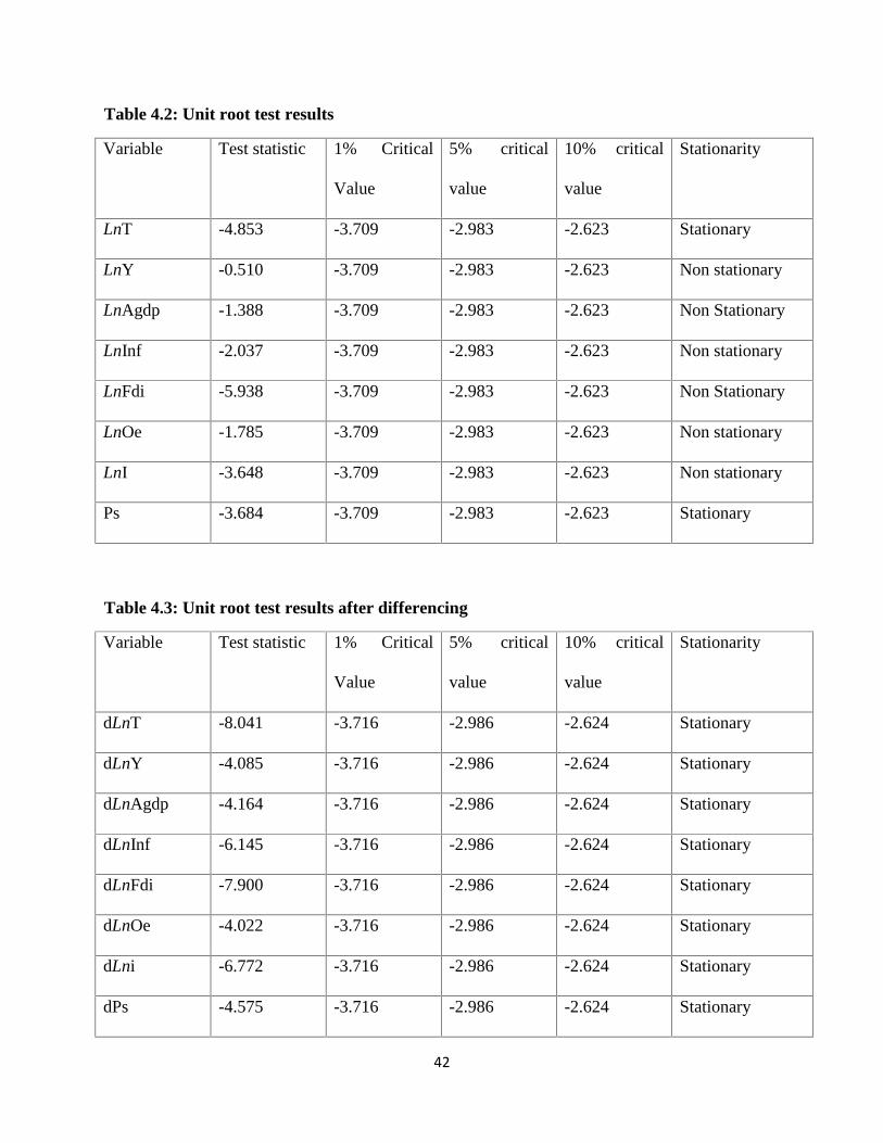
42

Table 4.2: Unit root test results

Variable Test statistic 1% Critical

Value

5% critical

value

10% critical

value

Stationarity

LnT -4.853 -3.709 -2.983 -2.623 Stationary

LnY -0.510 -3.709 -2.983 -2.623 Non stationary

LnAgdp -1.388 -3.709 -2.983 -2.623 Non Stationary

LnInf -2.037 -3.709 -2.983 -2.623 Non stationary

LnFdi -5.938 -3.709 -2.983 -2.623 Non Stationary

LnOe -1.785 -3.709 -2.983 -2.623 Non stationary

LnI -3.648 -3.709 -2.983 -2.623 Non stationary

Ps -3.684 -3.709 -2.983 -2.623 Stationary

Table 4.3: Unit root test results after differencing

Variable Test statistic 1% Critical

Value

5% critical

value

10% critical

value

Stationarity

dLnT -8.041 -3.716 -2.986 -2.624 Stationary

dLnY -4.085 -3.716 -2.986 -2.624 Stationary

dLnAgdp -4.164 -3.716 -2.986 -2.624 Stationary

dLnInf -6.145 -3.716 -2.986 -2.624 Stationary

dLnFdi -7.900 -3.716 -2.986 -2.624 Stationary

dLnOe -4.022 -3.716 -2.986 -2.624 Stationary

dLni -6.772 -3.716 -2.986 -2.624 Stationary

dPs -4.575 -3.716 -2.986 -2.624 Stationary

43

Since all the variable series have unit roots, it is possible that they are cointegrated thus the next

stage was to test for the possible existence of a cointegrating equation. This begins with the test

for multicollinearity.

4.3 Test for Multicollinearity

The table below presents the results of the test for multicollinearity among the variable series

data.

Table 4.4: Test for Multicollinearity

Variable VIF 1/VIF

DLnAgdp 1.45 0.687729

DLnY 1.35 0.740460

DPs 1.14 0.875338

DLnInf 1.13 0.883028

DLnI 1.12 0.892737

DLnFDI 1.12 0.895320

DLnOe 1.06 0.944740

Mean VIF 1.20

After first differencing all variables were tested for multicollinearity using Variance Inflation

Formula (VIF), since the VIF were all below 10. There was no problem of multicollinearity.

44

4.4 Autocorrelation test

The "Durbin-Watson test for autocorrelation'' is a statistic that indicates the likelihood that the

deviation (error) values for the regression have a first-order autoregression component. The

regression models assume that the error deviations are uncorrelated.

If the deviations are autocorrelated, there may be a number of consequences for the computed

results namely: The estimated regression coefficients may no longer have the minimum variance

property; the mean square error (MSE) may seriously underestimate the variance of the error

terms; and the computed standard error of the estimated parameter values may underestimate the

true standard error, in which case the t values and confidence intervals may be incorrect.

Small values of the Durbin-Watson statistic indicate the presence of autocorrelation. A value less

than 0.80 usually indicates that autocorrelation is likely. Initially .8199349 For our case, the

Durbin Watson statistic is 2.497682 this shows that there is no possible serial correlation

between the dependent variable and the residual of the estimated equations.

4.5 Co-integration test

The major concern with time series is that if non-stationarity of data series persists then it may

lead to spurious relationship. To avoid this problem, it is necessary to use the co-integration

methodology. The regression equation can be estimated for the period 1960-2010 using the

Engel-Granger two step procedure (Engel and Granger 1987). The first step is to estimate a long

run equation using ordinary least squares (OLS) with variables, which are integrated of order

one, I(1) in their levels. The results of the OLS with robust standard errors are shown in the table

4.5 below.

45

Table 4.5 OLS regression results

dlnT Coef. Robust

Std. Err.

t P>|t| 95%

Confidence

Interval

DlnY -0.970253 0.1888131 -0.51 0.612 -0.4867163 0.2926658

dlnAgdp -0.1959162 0.5680552 -0.34 0.733 -1.368325 0.9764921

dlnINF -0.335621 0.0238968 -1.40 0.173 -0.0828826 0.0157584

dlnFDI -0.218435 0.0117528 -1.86 0.075 -0.0461 0.0024131

dlnOe 0.0098658 0.1697539 0.06 0.954 -0.340489 0.3602207

Di -0.0720316 0.018804 -3.83 0.001 -0.1108411 -0.0332221

dPs -0.0268464 0.0192045 -1.40 0.175 -0.0664824 0.0127897

Cons 0.002324 0.0095488 0.24 0.810 -0.0173838 0.0220318

Number of observations = 32

F( 7, 24) = 2.55

Prob> F = 0.0411

R-squared = 0.4375

Root MSE = 0.04682

46

In order to avoid spurious regression, residual based cointegration test was used, where the

stationarity of the residual implies a cointegrating relationship among the variables in the long

run equation. The results for the ADF test of the residual are shown in the table 4.6.

Table 4.6: ADF test for residual

Test Statistic 1% Critical Value 5% Critical Value 10% Critical Value

Z(t) -6.964 -3.709 -2.983 -2.623

MacKinnon approximate p-value for Z(t) = 0.0000


Since the test statistic is -6.964 is less than the critical values at 1%, 5%, 10%, it therefore

implies that residual from the regression using the ADF test is stationary. This result indicates

that an ECM is a better fit than one without. The second step in the Engel Granger procedure is

to estimate the corresponding error correction model (ECM), based on the long run co-

integrating relationship to observe the short-run dynamics (Engel and Granger, 1987).

The study estimated the ECM using the residual from the long-run equation. The ECM is based

on stationary data (as all the I(1) regressors are in first difference form) and includes the lagged

residuals of the long-run equation, which is also I(0) when the variables have cointegrating

relationship. Since the dummy variable is not continuous, there is no need to worry about the

stationarity of the dummy variable. The study ran a short run error correction model (ECM). In

the ECM, the one period lagged residual for annual data acts as the error correction term. The

results of the error correction model in this case are presented in the table 4.7.

47

Table 4.7: Error Correction Model Results

dlnT Coef. Robust

Std. Err.

t P>|t| 95%

Confidence

Interval

dlnY -0.1652227 0.10503 -1.57 0.130 -0.3830415 0.0525962

dlnAgdp -0.3637257 0.2869408 -1.27 0.218 -0.9588043 0.231353

dlnINF -0.0433735 0.0103108 -4.21 0.000 -0.0647567 -0.0219902

dlnFDI -0.201954 0.0066467 -3.04 0.006 -0.0339799 -0.0064109

dlnOe 0.1241625 0.0806629 1.54 0.138 -0.0431221 .02914471

dlnI -0.552624 0.0117198 -4.72 0.00 -0.0795677 -0.030957

dPs -0.0104793 0.0080297 -1.31 0.205 -0.027132 0.0061734

dEct 0.5798868 0.0661129 8.77 0.00 0.4427771 0.7169966

_Cons 0.0037697 0.0056615 0.67 0.512 -0.0079716 0.015511


F( 8,22) = 23.73

Prob> F = 0.0000

R-squared = 0.8458

Root MSE = .02553

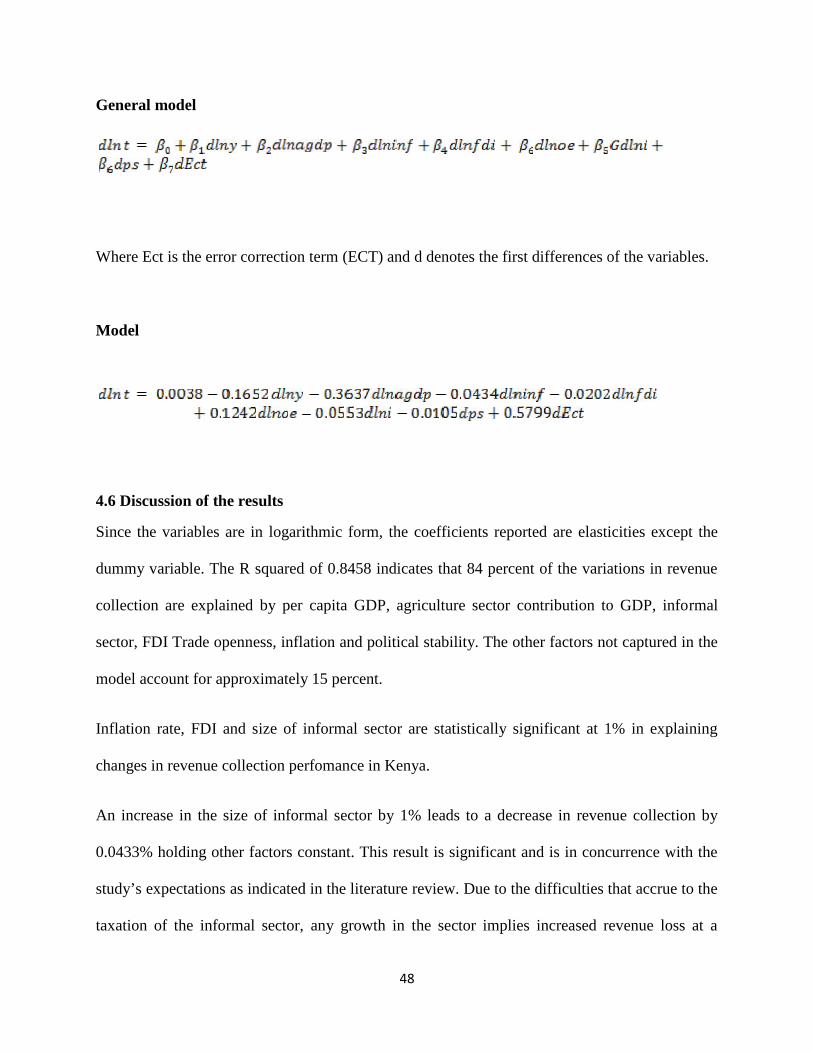
48

General model

Where Ect is the error correction term (ECT) and d denotes the first differences of the variables.

Model

4.6 Discussion of the results

Since the variables are in logarithmic form, the coefficients reported are elasticities except the

dummy variable. The R squared of 0.8458 indicates that 84 percent of the variations in revenue

collection are explained by per capita GDP, agriculture sector contribution to GDP, informal

sector, FDI Trade openness, inflation and political stability. The other factors not captured in the

model account for approximately 15 percent.

Inflation rate, FDI and size of informal sector are statistically significant at 1% in explaining

changes in revenue collection perfomance in Kenya.

An increase in the size of informal sector by 1% leads to a decrease in revenue collection by

0.0433% holding other factors constant. This result is significant and is in concurrence with the

study’s expectations as indicated in the literature review. Due to the difficulties that accrue to the

taxation of the informal sector, any growth in the sector implies increased revenue loss at a

48

General model


Model













48

General model


Model













49

statistically significant rate. Joshi et al. (2012) found that taxing the informal sector may not

yield much because the individual incomes are low while the costs of taxation are high.

Therefore, governments tend to leave this large sector alone. The informal sector is also a hiding

place for tax evaders who conceal themselves under the croak of informality while in actual fact

they should be in the taxable bracket. This is in concurrence with previous studies on the subject

matter. For instance Chipeta (2002) found the amount of revenue lost through tax evasion by

Malawi’s ‘second economy’ to be large and significant both in terms of potential revenue and

total actual revenue. Teera (2002) also found similar results, in that Uganda’s underground

economy was responsible for tax evasion that affected all the taxes. Cebula and Feige (2011) also

had similar results regarding the United States revenue losses due to unreported income by the

informal economy. This leads to the conclusion that fiscal policies need to be designed in order

to increase the cost of informality whilst at the same time giving incentives to the firms that opt

to voluntarily join the formal sector, with the ultimate objective of increasing the tax base.

The results indicate that a 1% increase in per capita GDP will lead to a decrease in total revenue

collection by 0.165% holding other factors constant. This is a surprising result, given the fact that

an increase in income per capita would imply a rise in taxable income which should improve tax

collection. However, it may be an indication that the increase in GDP per capita may be

accompanied by a higher wage expense for the formal sector, which has a negative impact on

corporation tax, thus making the net effect on tax collection negative. It may also imply tax

evasion by economic agents, with much of the taxable income going unreported or, in some

cases, through corruption. The result may also be because part of the period under study was

prior to the tax policy and modernization reforms whose effect was effectively felt in the late

1990’s, generally referred to as the post- tax reform era. A study by Muriithi and Moyi (2003)

50

established that buoyancy and tax to GDP elasticity in the post-reform era exceeded unity;

meaning tax growth was responsive to GDP growth. This was also the case in the findings of

Chelliah (1971) who concluded from his study that higher per capita income implies a higher

capacity to pay taxes as well as a greater capacity to collect them. The findings in this study

regarding the relationship between the tax collection and per capita income are therefore

surprising and warrant greater study in future.

Holding other factors constant, a rise in agriculture sector contribution to GDP by one percent

will lead to a decline in revenue collection by 0.3637% though this effect is not significant

statistically. This was similar to the findings by Ghura (1998), who found that revenue declined

with the share of Agriculture sector to GDP. This is likely to be as a result of the tax exemptions

and subsidies given by the government to the agricultural sector. Value addition in this sector is

low compared to other sectors of the economy, thus any revenue gains from an increase in

AGDP are likely to be negligible. This may also be due to the fact that most of the agricultural

activities are for subsistence, as well as political unwillingness by the government to tax this

sector as analyzed by Stotsky & WoldeMariam (1997) as well as Teera (2002).

The results show that an increase in FDI by 1% leads to a decrease in revenue collection by

0.020% holding other factors constant. This may be as a result of large tax holidays granted to

foreign investors especially in capital projects, as well as the long hiatus in capital gains tax.

With the re-introduction of capital gains tax, future increases in FDI may yield an increase in tax

revenue. Gupta (2007) found that capital gains tax significantly increases the revenue

performance in developing economies. However, due to Kenya’s country specific risk, the

government must be prudent in taxing capital growth, since investors require a risk premium for

51

their investment in the country in order to mitigate on any risk that may affect their return on

investment.

Holding other factors constant, an increase in the measure of trade openness by 1% leads to an

increase in revenue collection by 0.1242%. This is marginally significant at 10%. This is also

according to expectations, since increased international trade is likely to boost collection from

import duties and VAT. Keen and Simone (2004) made similar findings regarding the

relationship between revenue collection and international trade. It also implies a larger market

for local products, thus increasing the revenue base as firms expand production and profits. The

tax reforms that removed most export duties also made Kenya’s exports competitive in the global

market, thus inducing the production of goods for export and increasing the taxable income of

exporters. Export processing zones, manufacture under bond and other duty remission schemes

for goods imported for production of exports may also have contributed to this positive result in

taxable income from international trade. Gordon and Li (2009) also found in their study that the

developing countries on average still raise more than 16 per cent of government revenue from

border taxes, making trade openness vital for their economic growth.

Holding other factors constant an increase in the rate of inflation by 1% leads to a decrease in

revenue collection by 0.0553% though it is statistically insignificant. This may be as a result of

the fact that inflation diminishes real income, thus impacting negatively on trade and

profitability. It also affects firms in that unionized workers lobby for wage increases to mitigate

the effects of inflation, thus reducing the taxable income of firms. Inflation also creates “inflation

tax”, which when factored in may result in diminished tax revenue in real terms. A study by

OECD (2006) concluded that Kenya faces persistent inflation mainly due to oil prices which are

52

always rising, as well as regular droughts. Inflation also affects real interest rates, which drives

up the cost of borrowing and can negatively impact on economic growth, and hence revenue.

The dummy variable capturing effect of political stability is insignificant and implies that when

there is political instability i.e election years, the revenue collection goes down by approximately

0.0105%. The low level of significance indicates that there has not been any political instability

serious enough to cause real damage to the economy, and by extension, to the tax revenue

collection. However, this does not indicate that the political stability factor should be brushed

aside, since its ripple effects do adversely affect the economy, and by extension, tax revenue. A

study by the African Development Bank (2010) found out that the years of political turmoil

always negatively impacted on the Kenyan economy. These included the collapse of the East

African Community in 1977, the death of Mzee Jomo Kenyatta in 1978 and the attempted coup

in 1982. All these shook investor confidence and the rate of GDP growth was badly affected.

This too can be postulated in the case of the pre and post-election violence years covered by the

dummy variable in this study’s model.

The error correction term is significant and positive with a relatively high speed of adjustment of

about 0.57% suggesting that about 0.57% of deviations from long run equation are made up

within one time period.

53

CHAPTER FIVE

5.0 CONCLUSION AND POLICY RECOMMENDATIONS

5.1 Conclusion

Kenya has made great strides in the area of tax revenue collection. Tax reforms have increased

the efficiency in tax collection and made the country largely self sufficient in meeting the

government’s expenditure needs. The revenue collection agency, KRA, has made significant

progress in widening its tax base and has consistently reported growth in revenue since its

inception in 1995. However, the ballooning budget that has hit the Trillion shilling mark

necessitates renewed strategic thinking to avoid huge budget deficits which would lead to greater

indebtedness through domestic and foreign borrowing.

As the results of this study indicate, there are various determinants of revenue collection that

affect the efficiency of this activity. Variations in per capita GDP, agriculture sector contribution

to GDP, the informal sector, Foreign Direct Investment, Trade openness, inflation and political

stability account for approximately 85% of variations in tax revenue collection. The remaining

15% is accounted for by other factors outside the model, which are catered for by the error term.

The purpose of this study was to determine the effect of the growth in the informal sector on tax

revenue collection. The results indicate that an increase in the size of informal sector by 1%

would lead to a decrease in revenue collection by 0.0433% holding other factors constant. This

in effect means that a 100% increase in the size of the informal sector would lead to a 4.33%

decrease in tax revenue collection. If this was applied to the current KRA target of almost 1

Trillion in the 2013/2014 financial year, this would translate to around 40 Billion Kenya

Shillings tax loss. Given the rate of increase in the size of the informal economy as evidenced by

54

the consistent growth in employment in the sector, this kind of revenue loss is likely to grow in

arithmetic progression. This compares with past studies conducted in other countries, all of

which showed that growth in the informal sector has a corresponding negative effect on revenue

collection efforts. (Chipeta, 2002; Osoro, 1995; Rosser et al, 2000,2003)

Both the results of the study and the literature review reveal a compelling need by the fiscal

authorities to re-engineer the tax policies with a direct goal of tapping into the expansive

informal sector. Even though a large number of those employed in the informal sector falls

below the taxable bracket of Pay As You Earn tax, there exists many firms that operate

informally whose turn over and profits have tax implications. There is also the possibility that

much of the revenue is lost through loopholes in tax legislation and administration, thus the

government may need to enact stiffer penalties for tax evasion and improve the capacity of the

tax agency in order to carry out thorough audits and increase the cost of evading tax.

Bureaucratic hurdles of registration and payment of taxes should be minimized in order to

facilitate easier formalization of businesses.

Given the statistical significance of the results, fiscal policy decisions can be made on the basis

of projections done using the regression model in this study. This would necessarily include the

other variables considered in the model according to their respective significance levels. This is

especially so for per capita GDP and trade openness which in addition to the informal sector are

significant determinants of tax revenue performance.

55

5.2 Policy recommendations

Based on the findings of the study, fiscal authorities must take into consideration the magnitude

of the effects of the growth in the informal economy as well as variations in the other

determinants of tax revenue collection.

One of the policy measures necessary to cut revenue losses is formalization of the informal

sector. Although many of the so-called “jua kali” businesses are small enterprises, there exists a

considerable number of income generating ventures that should fall within the tax net. Kenya

Revenue Authority has in the recent past put in a great effort to ensure landlords declare rental

income for tax purposes. This effort includes the proposed mapping of all rental units in urban

areas by means of a Geo-spatial technology. This in effect is one measure to formalize the

housing sector which has largely been informally managed, especially where the landlords are

individuals and not firms. Advance tax for the passenger transport sector also reeled in matatu

operators into the tax net. Similar measures need to be instituted for other participants in the

informal economy such as timber merchants, vehicle garages, unregistered construction site

contractors, etc. Some of these businesses have a high sales turnover which could qualify for

VAT registration. Others have a large number of employees who fall within the PAYE bracket.

Through formulation of policies that give advantage to formal businesses over informal ones,

these firms are likely to opt for formalization, thus increasing the tax base. This also requires

firm political will as attempts to tax the informal sector are likely to be met with resistance and

hostility from sections of the public and their leaders. Tax amnesty for voluntary compliance is

also likely to catalyze the process of formalization of businesses for taxation purposes. The

literature reviewed also raises the issue of “psychic costs” of informality and tax evasion. Cebula

and Feige (2011) found out that the anxiety of being discovered and fined by the tax authorities

56

for tax evasion affected tax compliance by economic agents. This was increased by tax audits

and their yields, which in turn made tax evaders calculate their expected loss in case an audit was

carried out on their unreported income. Thus intensifying tax audits is likely to result in greater

compliance and formalization of qualifying firms and individuals.

With the current era of devolution in Kenya, a significant portion of tax collection has been

transferred from the national tax agency, KRA, to the county governments. It is also clearly

apparent that most of the revenue collected by county governments was from small and medium

enterprises located in rural localities and urban centers. This necessitates strategic thinking by

county governments in defining their fiscal policies, which necessarily must balance the issues of

social welfare, wealth redistribution and financial independence of individual counties. They

must also consider the issue of employment, such that they do not cause unemployment by over-

taxing small businesses. In this case, instead of the normal approach of instituting income taxes

and trade taxes in a generalized impersonal manner, the counties may opt to employ a ‘benefit

approach’ as enunciated by Musgrave and Musgrave (1989). This could either be through

general benefit taxes or specific benefit taxes. Specific benefit taxes are already in use in most

counties, and include user charges, tolls and fees. These are used where benefits accrue to a

particular consumer of a private good or service. The general benefit taxes are more complex

because they depend on individual preferences, and thus would depend on tax payers’ self

evaluation of their demand for social goods. The appropriate formula would therefore depend on

the income and price elasticity of demand for social goods, expressed by individual taxpayers’

indifference curves.

From the study, the results of other determinants also indicate the path that the government

should follow in order to increase the revenue performance. For instance, the Agriculture sector

57

contribution to GDP has a negative sign, indicating an inverse relationship with revenue

performance. To change this trend, policies that encourage value addition in the sector should be

formulated. This would see the rise of processing industries for agricultural output, which would

result in products that can be charged VAT on, as well as more profitable ventures that can yield

a substantial increase in corporation tax and payroll tax (PAYE). It would also change the

economy from a net importer to a net exporter, with exports of high value goods that can

compete favorably in the global market.

Trade openness (OE) has the expected positive sign. Import taxes and VAT contribute greatly to

the aggregate tax, and thus greater openness to international trade is likely to yield more revenue.

However, Kenya needs to move from being a primary producer to an industrialized economy in

order to gain comparative advantage in the international markets. This is especially so in the

regional market, namely in the East African Community and the COMESA trading bloc. By

moving from raw material production to selling finished goods, the Kenyan economy can greatly

benefit from the regional market where the removal of tariff and non-tariff barriers greatly

facilitate trade. This will, as a result lead to economic growth and better revenue performance.

An evaluation of Kenya’s benefit from international trade can also help formulate better trade

policies. The country should aim at moving from a net importer to a net exporter of finished

goods as set out in the Vision 2030 whose objective is to see the country move into a middle-

income economy. The results regarding Foreign Direct Investment show a negative sign, which

implies that an increase in FDI leads to a reduction in tax revenue. This would seem to support

the recent move by the government to reintroduce Capital Gains Tax, and thus this is the right

policy measure to reverse the revenue loss. The government should also encourage foreign

investors to engage in activities that enhance technological advancement and human capital

58

development, as opposed to employing expatriate workers. This is likely to lead to higher

productivity of capital and labour in the economy, and subsequently lead to higher tax yields.

The results also indicate that although of statistical insignificance, high inflation and political

instability negatively impact tax revenue performance. Therefore inflation control and a

favorable political climate create the proper environment for growth in tax revenue. The usual

inflation control mechanisms such as open market operations and price controls need to be

employed astutely to ensure tax growth. This is more so especially in crucial sectors that drive

the economy, such as the energy sector.

Income per capita is also a significant determinant of revenue performance. The negative sign

seems to indicate that though growth in per capita GDP is a desirable sign of economic growth

and development, it still impacts tax revenue collection negatively. In this respect, the

government needs to encourage a saving culture among the citizenry in order to stimulate growth

through investment. Although consumption increases as GDP per capita grows with the resultant

disposable income, increased saving is likely to be more beneficial to the economy since the

savings can be used to fund industrial growth, business expansion and infrastructural

development which in effect would lead to an increase in taxable income.

Among the variety of measures available for the government to increase tax revenue from the

informal sector, there are two that stand out from a study by Joshi (2012). The first one is called

the Block Management System (BMS) which is practiced in Tanzania. According to Joshi, the

BMS is set up so that trading areas are mapped and divided into blocks on the basis of geography,

administrative boundaries or a few streets. Each block is mandated to operate all tax functions of

identification, registration, assessing and accounting for revenue collected, with the BMS team

59

allocated a team of staff with relevant skills to perform these functions. This involves door to

door taxpayer recruitment and follow up within the set blocks. This system helps to zero in on

the small and medium enterprise which would normally hide under the cloak of anonymity. The

second option is the Associational Taxation which is practiced in Ghana. Joshi states that such a

strategy implies proactive efforts to foster effective collective action within the informal sector,

coupled with the creation of institutional channels to facilitate bargaining and cooperation

between informal sector associations and the state. This brings about acceptance by the business

community, increases compliance and reduces tax collection costs to a fixed minimum.

Finally, there are other factors that determine tax revenue performance but which are not covered

by this paper. This study therefore raises further questions in the area of taxation, and

recommends further research on the determinants of tax revenue performance as well as the

impact of the growth of the informal sector on the Kenyan economy.

60

REFERENCES

Ahumada, H., Alvaredo, F. and Canavese, A. (2008). ‘The Monetary Method to Measure theShadow Economy: The Forgotten Problem of the Initial Conditions’, Economics Letters Vol.101.

Alm, James (1985), ‘The Welfare Cost of the Underground Economy. Economic Inquiry, Vol.24.

Andreoni, J., Erard, B. and Feinstein J. (1998). ‘Tax Compliance’, Journal of EconomicLiterature Vol.36.

Atieno, R (2006). ‘Female participation in the labour market: The case of the informal sector in

Kenya’, AERC Research paper series, No. 157, Nairobi, Africa Economic Research Consortium.

Bahl, R.W. (2003). ‘Reaching the Hardest to Tax: Consequences and Possibilities’, paperpresented at the “Hard to Tax: An International Perspective” conference, Andrew Young Schoolof Policy Studies, Georgia State University, USA.

Breusch, T. (2005). ‘Australia's Cash Economy: Are the Estimates Credible?’ a presentation atthe Australian National University.

Cebula, R. and Feige, E. (2011). ‘America’s underground economy: Measuring the size, growthand determinants of income tax evasion in the U.S’, SSC-WISC Website, www.ssc.wisc.edu

Cheeseman, N. And Griffiths R, (2006) ‘Increasing tax revenue in sub-Saharan Africa: The caseof Kenya’, Economy Analysis Paper series, No.6, The Oxford Council of Good Governance,Oxford, UK.

Chen, M., Vanek, J. Lund, F., Heintz, J., Jhabvala, R., Bonner, C. (2005) ‘Progress of theworld’s women: Women, work and poverty’, New York, UNIFEM.

Chong, A. and M. Gradstein (2004), “Inequality, institutions and informality”, IDB WorkingPaper Series, No. 516, Inter-American Development Bank.

Chipeta, C. (2002), ‘The second economy and tax yield in Malawi’, AERC Research paper

series, No.113, Nairobi, Africa Economic Research Consortium.

Das-Gupta, A. (1994) ‘A Theory of Hard-to-Tax Groups’, Public Finance, Vol.49 (Supplement).

De Soto, H. (1989) The other path: The invisible revolution in the Third World, IB TaurisPublishers, London, UK.

61

DFID (2004). Kenya: Country Assistance Plan 2004 – 2007, London, Department forInternational Development.

Dickey, D.A. and Fuller, D.A. (1979). ‘Distributions of the Estimators for Autoregressive TimeSeries with a Unit Root’, Journal of American Statistical Association, Vol. 74, No. 366.

Eissa, N. and Jack, W. (2009) ‘Tax Reform in Kenya: Policy and administrative issues’, IPD

working paper series, Initiative for policy dialogue, Columbia University.

Feige, E. (1979). ‘How Big is the Irregular Economy?’ Challenge series, Vol.20.

Feige, E. and Urban, I. (2008) ‘Measuring Underground (Unobserved, Non-Observed,Unrecorded) Economies in Transition Countries: Can We Trust GDP?’, Journal of ComparativeEconomics Vol. 36.

Friedman, E., Johnson, S., Kaufmann, D. and Zoido-Lobaton, P. (2000) ‘Dodging the GrabbingHand: The Determinants of Unofficial Activity in 69 Countries’, Journal of Public EconomicsVol. 76.

Gelb, A. (1993). “Socialist Transformations: Some Lessons and Implications for Assistance”. InSIDA Redefining the Role of the State and the Market in the Developing Process, Skara,Vastergot Lands, Tryckeri.

Ghura, Dhaneshwar, (1998). 'Tax Revenue in Sub saharan Africa: Effects of Economic POliciesand Corruption,' IMF Working Paper Series, No. 98/135, Washington, International MonetaryFund.

Gordon, R. and Li, W. (2009). ‘Tax Structures in Developing Countries: Many Puzzles and aPossible Explanation’, Journal of Public Economics, Vol.93.

Gupta, A. (2007). ‘Determinants of tax revenue efforts in developing countries’, International

Monetary Fund Working Paper Series, No. WP/07/184, UCSC Website, www.ucsc.edu

Gutmann, P. (1977). ‘The Subterranean Economy’, Financial Analysts Journal Vol.33.

International Labor Organization (2012), Measuring Informality: A statistical manual on

informal sector and informal employment, ILO, Geneva, Switzerland.

62

Johnson, S., D. Kaufmann and P. Zoido-Lobaton (1998). ‘Regulatory discretion and theunofficial economy’, American Economic Review: Papers and Proceedings, No.88.

Joshi, A., Prichard, W., Heady, C. (2012), ‘Taxing the informal economy: Challenges,possibilities and remaining questions’, ICTD Working Paper Series, No. 4, International Centrefor Tax and Development, Brighton, UK, Institute of Development Studies.

Kaldor, N. (1964). ‘Will Underdeveloped Countries Learn How to Tax?’ Essays on EconomicPolicy, Vol.1, London, UK, Gerald Duckworth & Company Limited.

Karingi, S., Wanjala, A., Kamau, A., Nyakang’o, E., Mwangi, A., Muhoro, M., and Nyamunga,J. (2004). “Fiscal Architecture and Revenue Capacity in Kenya.” KIPPRA Discussion PaperSeries, No. DP/45/2004. Nairobi, Kenya Institute for Public Policy Research and Analysis.

Kaufmann, D. and Kaliberda, A. (1996) ‘Integrating the Unofficial Economy into the Dynamicsof Post-Socialist Economies: A Framework of Analysis and Evidence’, World Bank PolicyResearch Working Paper Series, No. 1691. Washington, DC, World Bank.

Keen, M. (2012) ‘Tax and Development – Again’, in G. Zodrow and C. Fuest, Taxation inDeveloping Countries. Cambridge MA, MIT Press.

Kenadjian, B. (1982). ‘The Direct Approach to Measuring the Underground Economy in theUnited States: IRS Estimates of Unreported Income,’ in Vito Tanzi, ed., The UndergroundEconomy in the United States and Abroad. Lexington, MA and Toronto: Lexington Books.

Levenson, A. R. And Maloney, W. (1998), ‘The informal sector, firm dynamics and institutionalparticipation’, World Bank Policy Research Working Paper Series, No. 1988. Washington, DC,World Bank.

Lindbeck, Assar. (1980). ‘Tax Effects versus Budget Effects on Labour Supply’ SIIES Seminarpaper, No. 148. Stockholm, Sweden, Stockholm Institute for International Economic Studies.

Loayza, N. (1997) ‘The Economics of the Informal Sector. A simple model and some empiricalevidence from Latin America’. World Bank Policy Research Working Paper Series, No. 1727.Washington, DC, World Bank.

Lotz, J.R. and Morss, E.R. (1967). ‘Measuring Tax Effort in Developing Countries’,International Monetary Staff Papers Series, Vol.14.

Martinez-Vazquez, Jorge (1996). “Who Benefits from Tax Evasion? The Incidence of TaxEvasion” Public Economics Review, Vol.1.

63

Muchiri, B. and Audi, P. (2007) ‘Statistical measures of growth and their changes over time’

KNBS online Publication, Kenya National Bureau of Statistics website, www.knbs.go.ke

Muriithi, M. K. and Moyi, E. (2003). ‘Tax Reforms and Revenue Mobilization in Kenya’, AERCResearch Paper Series, No. 131, Nairobi, Africa Economic Research Consortium.

Musgrave. R. and Musgrave. P. (1989). Fiscal systems, McGraw-HILL Book company,Singapore.

OECD (2006). “African Economic Outlook”, OECD Website, www.oecd.org

Ogutu, P. C., (2013). ‘Informal sector taxation in Kenya; Issues and policy options – Informalsector perspective’, a presentation by National Informal Sector Coalition, Nairobi, Kenya.

Ole, A.M. (1975). ‘Income Elasticity of Tax Structure in Kenya: 1962/63-1972/73’,Unpublished. M.A Research Paper, University of Nairobi.

OREA (2010). ‘Domestic Resource Mobilization for Poverty Reduction in East Africa: KenyaCase Study’, African Development Bank Group, Regional Department East Africa.

Osoro, N (1995). ‘Tax reforms in Tanzania: Motivations, Directions and Implications’, AERC

Research paper Series, No. 62, Nairobi, Kenya. Africa Economic Research Consortium.

Palda, Filip (1998). ‘Evasive Ability and the Efficiency Cost of the Underground Economy.’ TheCanadian Journal of Economics, Vol.31.

Pimhidzai and Fox, L. (2012). ‘Taking from the Poor or Local Economic Development: TheDilemma of Taxation of Small Informal Enterprises in Uganda’, CSAE Working Paper,Washington DC, The World Bank.

Prest, A.R. (1975), Public Finance in Developing Countries, Weidenfeld and Nicholson,

London.

Republic of Kenya, (1965). ‘African Socialism and its Application to Planning in Kenya’Sessional Paper No. 10 of 1965. Nairobi, Government printer.

Republic of Kenya, (1986). ‘Economic Management for Renewed Growth’ Sessional Paper No.1 of 1986, Nairobi, Government printer.

64

Republic of Kenya, (1994). National Development Plan 1994 - 1996. Nairobi: Governmentprinter.

Republic of Kenya, (1994). ‘Recovery and Sustainable Development to the Year 2010’ SessionalPaper No. 1 of 1994 Nairobi: Government printer.

Rosser, J. B., Rosser, M and Ahmed, E. (2000). ‘Income inequality and the informal economy intransition economies’, Journal of Comparative Economics, Vol.28.

Rosser, J. B., Rosser, M and Ahmed, E. (2003). ‘Multiple unofficial economy equilibria andincome distribution dynamics in systemic transition’, Journal of Post Keynesian Economics,Vol.25.

Schneider, F. and Enste, D. (2000). ‘Shadow Economies: Sizes, Causes and Consequences’,Journal of Economic Literature Vol.38.

Stotsky, J.G. and WoldeMariam, A. (1997), ‘Tax Effort in Sub-Saharan Africa’, IMFWorking Paper Series, No.WP/97/107, Washington DC, International Monetary Fund.

Tanzi, V. (1987). Quantitative Characteristics of the Tax System of Developing Countries. TheTheory of Taxation for Developing Countries, New York, Oxford University Press

Tanzi, V. (1999) ‘Uses and Abuses of Estimates of the Underground Economy’, EconomicJournal Vol.109.

Teera, J.M. (2002). ‘Determinants of Tax Revenue Share in Uganda’ (unpublished researchpaper)

Terkper, Seth (2003). ‘Managing Small and Medium-Size Taxpayers in Developing Economies.’Tax Notes International, 13 January 2003.

Thomas, J. (1999) ‘Quantifying the Black Economy: Measurement Without Theory Yet Again?’Economic Journal, Vol.109.

Toye, J.F.J. (1978). (Ed.), Taxation and Economic Development, London, England: Frank Cass& Co. Ltd.

Vuletin, G. (2008) ‘Measuring the Informal Economy in Latin America and the Caribbean’, IMFWorking PaperSeries, No. 102. Washington, DC, International Monetary Fund.

Wawire, N. H. W. (1991). ‘An Empirical Assessment of Tax Performance in Kenya: 1958 –1989’, M.A. Research Paper, Kenyatta University.

65

Wawire, N. H. W. (2000). ‘Revenue Productivity Implications of Kenya’s Tax System’ inKwaaPrah, K. and A. G. M. Ahmed (Ed.). Africa in Transformation.Political and EconomicIssues.Vol. 1. Addis Ababa, OSSREA.

Wawire, N. H. W. (2003). ‘Trends in Kenya’s Tax Ratios and Tax Effort Indices, and TheirImplication for Future Tax Reforms’ in Illieva E. V. (Ed.) Egerton Journal, Vol.4.

Wilford, S.D. and Wilford, W. (1978). ‘Estimates of Revenue Elasticity and Buoyancy in CentralAmerica: 1955- 1974’ in Toye, J.F.J (Ed.), Taxation and Economic Development. London, FrankCass & Co. Ltd.

World Bank (2006). “Kenya inside Informality: poverty, jobs, housing and services in Nairobi’sslums”, World Bank Report no.36347-KE, Washington, DC, World Bank.

Yitzhaki, Shlomo (1987). “On the Excess Burden of Tax Evasion.” Public Finance Quarterly,Vol.15.

An analysis of the effect of the growth of the informal ...

Documents

Transcript of An analysis of the effect of the growth of the informal ...