
An Analysis of Global Positioning System (GPS) Standard ... · An Analysis of Global Positioning...
105
An Analysis of Global Positioning System (GPS) Standard Positioning System (SPS) Performance for 2015 TR-SGL-17-04 March 2017 Space and Geophysics Laboratory Applied Research Laboratories The University of Texas at Austin P.O. Box 8029 Austin, TX 78713-8029 Brent A. Renfro, Jessica Rosenquest, Audric Terry, Nicholas Boeker Contract: NAVSEA Contract N00024-01-D-6200 Task Order: 5101147 Distribution A: Approved for public release; Distribution is unlimited.
Transcript of An Analysis of Global Positioning System (GPS) Standard ... · An Analysis of Global Positioning...
An Analysis of Global PositioningSystem (GPS) StandardPositioning System (SPS)Performance for 2015
TR-SGL-17-04
March 2017
Space and Geophysics LaboratoryApplied Research Laboratories
The University of Texas at AustinP.O. Box 8029
Austin, TX 78713-8029
Brent A. Renfro,Jessica Rosenquest,
Audric Terry,Nicholas Boeker
Contract: NAVSEA Contract N00024-01-D-6200Task Order: 5101147
Distribution A: Approved for public release; Distributionis unlimited.

This Page Intentionally Left Blank

Executive Summary
Applied Research Laboratories, The University of Texas at Austin (ARL:UT) examinedthe performance of the Global Positioning System (GPS) throughout 2015 for theGlobal Positioning Systems Directorate (SMC/GP). This report details the results ofthat performance analysis. This material is based upon work supported by the US AirForce Space & Missile Systems Center Global Positioning Systems Directorate throughNaval Sea Systems Command Contract N00024-01-D-6200, task order 5101147, “FY15GPS Signal and Performance Analysis”.
Performance is defined by the 2008 Standard Positioning Service (SPS) PerformanceStandard (SPS PS). The performance standards provide the U.S. government’sassertions regarding the expected performance of GPS. This report does not addresseach of the assertions in the performance standards. This report emphasizes thoseassertions which can be verified by anyone with knowledge of standard GPS dataanalysis practices, familiarity with the relevant signal specification, and access to aGlobal Navigation Satellite System (GNSS) data archive.
The assertions evaluated include those of accuracy, integrity, continuity, and availabilityof the GPS signal-in-space (SIS) and the position performance standards. Chapter 2 ofthe report includes a tabular summary of the assertions that were evaluated and asummary of the results. The remaining Chapters present details on the analysisassociated with each assertion.
All the SPS PS metrics examined in the report were met in 2015.
Contents
1 Introduction 1
2 Summary of Results 4
3 Discussion of Performance Standard Metrics and Results 6
3.1 SIS Accuracy . . . . . . . . . . . . . . . . . . . . . . . . . . . . . . . . . 6
3.1.1 URE Over All AOD . . . . . . . . . . . . . . . . . . . . . . . . . 8
3.1.1.1 An Alternate Approach . . . . . . . . . . . . . . . . . . 12
3.1.2 URE at Any AOD . . . . . . . . . . . . . . . . . . . . . . . . . . 12
3.1.3 URE at Zero AOD . . . . . . . . . . . . . . . . . . . . . . . . . . 20
3.1.4 URE Bounding . . . . . . . . . . . . . . . . . . . . . . . . . . . . 20
3.1.5 UTC Offset Error Accuracy . . . . . . . . . . . . . . . . . . . . . 21
3.2 SIS Integrity . . . . . . . . . . . . . . . . . . . . . . . . . . . . . . . . . . 21
3.2.1 URE Integrity . . . . . . . . . . . . . . . . . . . . . . . . . . . . . 21
3.2.2 UTCOE Integrity . . . . . . . . . . . . . . . . . . . . . . . . . . . 23
3.3 SIS Continuity . . . . . . . . . . . . . . . . . . . . . . . . . . . . . . . . 23
3.3.1 Unscheduled Failure Interruptions . . . . . . . . . . . . . . . . . . 23
3.3.2 Status and Problem Reporting Standards . . . . . . . . . . . . . . 27
3.3.2.1 Scheduled Events . . . . . . . . . . . . . . . . . . . . . . 27
3.3.2.2 Unscheduled Outages . . . . . . . . . . . . . . . . . . . 29
3.3.2.3 Suspect NANUs . . . . . . . . . . . . . . . . . . . . . . 30
3.4 SIS Availability . . . . . . . . . . . . . . . . . . . . . . . . . . . . . . . . 31
3.4.1 Per-slot Availability . . . . . . . . . . . . . . . . . . . . . . . . . 31
3.4.2 Constellation Availability . . . . . . . . . . . . . . . . . . . . . . 31
3.4.3 Operational Satellite Counts . . . . . . . . . . . . . . . . . . . . . 33
i
3.5 Position/Time Domain Standards . . . . . . . . . . . . . . . . . . . . . . 35
3.5.1 PDOP Availability . . . . . . . . . . . . . . . . . . . . . . . . . . 35
3.5.2 Additional DOP Analysis . . . . . . . . . . . . . . . . . . . . . . 36
3.5.3 Position Service Availability . . . . . . . . . . . . . . . . . . . . . 44
3.5.4 Position Accuracy . . . . . . . . . . . . . . . . . . . . . . . . . . . 44
3.5.4.1 Results for Daily Average . . . . . . . . . . . . . . . . . 48
3.5.4.2 Results for Worst Site 95th Percentile . . . . . . . . . . . 52
4 Additional Results of Interest 56
4.1 Frequency of Different SV Health States . . . . . . . . . . . . . . . . . . 56
4.2 Age of Data . . . . . . . . . . . . . . . . . . . . . . . . . . . . . . . . . . 56
4.3 User Range Accuracy Index Trends . . . . . . . . . . . . . . . . . . . . . 59
4.4 Extended Mode Operations . . . . . . . . . . . . . . . . . . . . . . . . . 60
A URE as a Function of AOD 64
A.1 Notes . . . . . . . . . . . . . . . . . . . . . . . . . . . . . . . . . . . . . . 65
A.2 Block IIA SVs . . . . . . . . . . . . . . . . . . . . . . . . . . . . . . . . . 66
A.3 Block IIR SVs . . . . . . . . . . . . . . . . . . . . . . . . . . . . . . . . . 67
A.4 Block IIR-M SVs . . . . . . . . . . . . . . . . . . . . . . . . . . . . . . . 70
A.5 Block IIF SVs . . . . . . . . . . . . . . . . . . . . . . . . . . . . . . . . . 72
B URE Analysis Implementation Details 75
B.1 Introduction . . . . . . . . . . . . . . . . . . . . . . . . . . . . . . . . . . 75
B.2 Clock and Position Values for Broadcast and Truth . . . . . . . . . . . . 75
B.3 95th Percentile Global Average As Per the SPS PS . . . . . . . . . . . . . 76
B.4 An Alternate Approach . . . . . . . . . . . . . . . . . . . . . . . . . . . . 77
B.5 Limitations of URE Analysis . . . . . . . . . . . . . . . . . . . . . . . . . 79
C SVN to PRN Mapping for 2015 80
D NANU Activity in 2015 82
E SVN to Plane-Slot Mapping for 2015 84
F Translation of URE Statistics Between Signals 88
ii

F.1 Group Delay Differential . . . . . . . . . . . . . . . . . . . . . . . . . . . 88
F.2 Intersignal Bias . . . . . . . . . . . . . . . . . . . . . . . . . . . . . . . . 89
F.3 Adjusting PPS dual-frequency Results for SPS . . . . . . . . . . . . . . . 90
G Acronyms and Abbreviations 91
iii

List of Figures
1.1 Maps of the Network of Stations Used as Part of this Report . . . . . . . 3
3.1 Range of the Monthly 95th Percentile Values for All SVs . . . . . . . . . 11
3.2 Range of the Monthly 95th Percentile Values for all SVs (via AlternateMethod) . . . . . . . . . . . . . . . . . . . . . . . . . . . . . . . . . . . . 14
3.3 Range of Differences in Monthly Values for all SVs . . . . . . . . . . . . 14
3.4 Worst Performing Block IIA SV in Terms of Any AOD (SVN 40/PRN 10) 17
3.5 Worst Performing Block IIR/IIR-M SV in Terms of Any AOD (SVN44/PRN 28) . . . . . . . . . . . . . . . . . . . . . . . . . . . . . . . . . . 17
3.6 Worst Performing Block IIF SV in Terms of Any AOD (SVN 65/PRN 24) 18
3.7 Best Performing Block IIA SV in Terms of Any AOD (SVN 23/PRN 32) 18
3.8 Best Performing Block IIR/IIR-M SV in Terms of Any AOD (SVN 60/PRN23) . . . . . . . . . . . . . . . . . . . . . . . . . . . . . . . . . . . . . . . 19
3.9 Best Performing Block IIF SV in Terms of Any AOD (SVN 63/PRN 01) 19
3.10 Daily Average Number of Occupied Slots . . . . . . . . . . . . . . . . . . 33
3.11 Count of Operational SVs by Day . . . . . . . . . . . . . . . . . . . . . . 34
3.12 Daily PDOP Metrics Using all SVs, 2015 . . . . . . . . . . . . . . . . . . 39
3.13 Daily PDOP Metrics Using All SVs, 2013 . . . . . . . . . . . . . . . . . . 40
3.14 Daily PDOP Metrics Using All SVs, 2014 . . . . . . . . . . . . . . . . . . 40
3.15 GPS Visibility on Day 035 at 01:11 Relative to 63N, 36.44E . . . . . . . 43
3.16 Daily Averaged Position Residuals Computed Using a RAIM Solution . . 50
3.17 Daily Averaged Position Residuals Computed Using No Data Editing . . 50
3.18 Daily Averaged Position Residuals Computed Using a RAIM Solution (en-larged) . . . . . . . . . . . . . . . . . . . . . . . . . . . . . . . . . . . . . 51
3.19 Daily Averaged Autonomous Position Residuals Computed Using No DataEditing (enlarged) . . . . . . . . . . . . . . . . . . . . . . . . . . . . . . . 51
iv

3.20 Worst Site 95th Daily Averaged Position Residuals Computed Using aRAIM Solution . . . . . . . . . . . . . . . . . . . . . . . . . . . . . . . . 54
3.21 Worst Site 95th Daily Averaged Position Residuals Computed Using NoData Editing . . . . . . . . . . . . . . . . . . . . . . . . . . . . . . . . . 54
4.1 Constellation Age of Data for 2015 . . . . . . . . . . . . . . . . . . . . . 59
B.1 Global Average URE as defined in SPS PS . . . . . . . . . . . . . . . . . 76
B.2 Illustration of the 577 Point Grid . . . . . . . . . . . . . . . . . . . . . . 78
C.1 PRN to SVN Mapping for 2015 . . . . . . . . . . . . . . . . . . . . . . . 81
D.1 Plot of NANU Activity for 2015 . . . . . . . . . . . . . . . . . . . . . . . 83
E.1 Time History of Satellite Plane-Slots for 2015 . . . . . . . . . . . . . . . 87
v

List of Tables
2.1 Summary of SPS PS Metrics Examined for 2015 . . . . . . . . . . . . . . 5
3.1 Characteristics of SIS URE Methods . . . . . . . . . . . . . . . . . . . . 7
3.2 Monthly 95th Percentile Values of SIS RMS URE for All SVs . . . . . . . 10
3.3 Monthly 95th Percentile Values of SIS Instantaneous URE for all SVs (viaAlternate Method) . . . . . . . . . . . . . . . . . . . . . . . . . . . . . . 13
3.4 95th Percentile Global Average UTCOE for 2015 . . . . . . . . . . . . . . 22
3.5 Probability Over Any Hour of Not Losing Availability Due to UnscheduledInterruption . . . . . . . . . . . . . . . . . . . . . . . . . . . . . . . . . . 26
3.6 Scheduled Events Covered in NANUs for 2015 . . . . . . . . . . . . . . . 28
3.7 Decommissioning Events Covered in NANUs for 2015 . . . . . . . . . . . 29
3.8 Unscheduled Events Covered in NANUs for 2015 . . . . . . . . . . . . . . 30
3.9 Per-Slot Availability in 2015 for Baseline 24 Slots . . . . . . . . . . . . . 32
3.10 Summary of PDOP Availability . . . . . . . . . . . . . . . . . . . . . . . 36
3.11 Additional DOP Annually-Averaged Visibility Statistics for 2012 through2015 . . . . . . . . . . . . . . . . . . . . . . . . . . . . . . . . . . . . . . 38
3.12 Additional PDOP Statistics . . . . . . . . . . . . . . . . . . . . . . . . . 38
3.13 Satellite and NANUs Associated with Single-Day Large DOP Values . . . 41
3.14 DOP Results for 63N, 36.44E on Day 34/35 . . . . . . . . . . . . . . . . 42
3.15 Organization of Positioning Results . . . . . . . . . . . . . . . . . . . . . 47
3.16 Mean of Daily Average Position Errors for 2015 . . . . . . . . . . . . . . 49
3.17 Median of Daily Average Position Errors for 2015 . . . . . . . . . . . . . 49
3.18 Maximum of Daily Average Position Errors for 2015 . . . . . . . . . . . . 49
3.19 Standard Deviation of Daily Average Position Errors for 2015 . . . . . . 49
3.20 Mean of Daily Worst Site 95th Percentile Position Errors for 2015 . . . . 55
3.21 Median of Daily Worst Site 95th Percentile Position Errors for 2015 . . . 55
vi

3.22 Maximum of Daily Worst Site 95th Percential Position Errors for 2015 . . 55
3.23 Standard Deviation of Daily Worst Site 95th Percentile Position Errors for2015 . . . . . . . . . . . . . . . . . . . . . . . . . . . . . . . . . . . . . . 55
4.1 Frequency of Health Codes . . . . . . . . . . . . . . . . . . . . . . . . . . 57
4.2 Age of Data of the Navigation Message by SV Type . . . . . . . . . . . . 58
4.3 Distribution of URA Index Values . . . . . . . . . . . . . . . . . . . . . . 61
4.4 Distribution of URA Index Values As a Percentage of All Collected . . . 62
4.5 Summary of Occurrences of Extended Mode Operations . . . . . . . . . . 63
E.1 Summary of SV-Slot Relationships for 2015 . . . . . . . . . . . . . . . . 86
G.1 List of Acronyms and Abbreviations . . . . . . . . . . . . . . . . . . . . 91
vii
Chapter 1
Introduction
Applied Research Laboratories, The University of Texas at Austin (ARL:UT)1
examined the performance of the Global Positioning System (GPS) throughout 2015 forthe Global Positioning Systems Directorate (SMC/GP). This report details the resultsof our performance analysis. This material is based upon work supported by the US AirForce Space & Missile Systems Center Global Positioning Systems Directorate throughNaval Sea Systems Command Contract N00024-01-D-6200, task order 5101147, “FY15GPS Signal and Performance Analysis”.
Performance is assessed relative to selected assertions in the 2008 Standard PositioningService (SPS) Performance Standard (SPS PS) [1]. (Hereafter the term SPS PS, orSPSPS08, are used when referring to the 2008 SPS PS.) Chapter 2 contains a tabularsummary of performance stated in terms of the metrics provided in the performancestandard. Chapter 3 contains explanations and amplifications regarding the summaryvalues. Chapter 4 details additional findings of the performance analysis.
The performance standards define the services delivered through the L1 C/A codesignal. The metrics are limited to characterizing the signal in space (SIS) and do notaddress error sources such as atmospheric errors, receiver errors, or error due to theuser environment (e.g. multipath errors, terrain masking, and foliage). This reportaddresses assertions in the SPS PS that can be verified by anyone with knowledge ofstandard GPS data analysis practices, familiarity with the relevant signal specification[2], and access to a data archive (such as that available via the International GlobalNavigation Satellite System (GNSS) Service (IGS)) [3]. The assertions examinedinclude those related to user range error (URE), availability of service, and positiondomain standards (specifics can be found in Table 2.1).
The majority of the assertions related to URE values are evaluated through comparisonof the space vehicle (SV) clock and position representations as computed from thebroadcast Legacy Navigation (LNAV) message data against the SV truth clock andposition data as provided by a precise orbit calculated after the time of interest. Thebroadcast clock and position data is denoted in this report by BCP and the truth clock
1A complete list of abbreviations found in this document is provided in Appendix G.
1

GPS SPS Performance Analysis 2015
and position data by TCP. The process by which the URE values are calculated isdescribed in Appendix B of this report.
Observation data from tracking stations are used to cross-check the URE values and toevaluate non-URE assertions. Examples of the latter application include the areas ofContinuity (3.3), Availability (3.4), and Position/Time Availability (3.5). In thesecases, data from two networks are used. The two networks considered are the NationalGeospatial-Intelligence Agency (NGA) Monitor Station Network (MSN) [4] and asubset of the tracking stations that contribute to the IGS. The distribution of thesestations is shown in Figure 1.1. These sets of stations ensure continuous observation ofall space vehicles by multiple stations.
Several metrics in the performance standards are stated in terms of the Base 24constellation of six planes and four slots/plane or the Expandable 24 constellation inwhich three of the 24 slots may be occupied by two SVs. Currently, there are morethan 32 GPS SVs on-orbit. Of these, at most 31 SVs may be operationallybroadcasting at any time. Of the SVs on-orbit, 27 are located in the expandable 24constellation. The SVs in excess of those located in defined slots are assigned tolocations in various planes in accordance with operational considerations.
The majority of the metrics in this report are evaluated on either a per-SV basis or forthe full constellation. The metrics associated with continuity and availability aredefined with respect to the slot definitions.
The GPS SVs are referred to by pseudo-random noise ID and by space vehicle number(referred to hereafter as PRN and SVN, respectively). As the number of active PRNshas increased to nearly the total available number, PRNs are now being used bymultiple SVs within a given year (but by no more than one SV at a time). Therefore,the SVN represents the permanent unique identifier for the vehicle under discussion. Ingeneral, we list the SVN first and the PRN second because the SVN is the uniqueidentifier of the two. The SVN-to-PRN relationships were provided by the MasterControl Station (MCS), however another useful summary of this information may befound on the U.S. Naval Observatory (USNO) website [5].
The authors acknowledge and appreciate the effort of several ARL:UT staff memberswho reviewed these results. For 2015 this included Shannon Kolensky, Scott Sellers,and Johnathan York.
Karl Kovach of Aerospace provided valuable assistance in interpreting the SPSPS08metrics. John Lavrakas of Advanced Research Corporation and P.J. Mendicki ofAerospace Corporation have long been interested in GPS performance metrics andprovided comments on the final draft. Their inputs were very valuable. However, theresults presented in this report are derived by ARL:UT, and any errors are theresponsibility of ARL:UT.
2

GPS SPS Performance Analysis 2015
Figure 1.1: Maps of the Network of Stations Used as Part of this Report
3
Chapter 2
Summary of Results
Table 2.1 is a summary of the assertions defined in the performance standards. Thetable is annotated to show which assertions are evaluated in this report and the statusof each assertion that was evaluated.
All the SPS PS metrics examined in the report were met in 2015.
Details regarding each result may be found in Chapter 3.
4

GPS SPS Performance Analysis 2015
Table 2.1: Summary of SPS PS Metrics Examined for 2015
SPSPS08 Section SPS PS Metric 2015 Status
3.4.1 SIS URE Accuracy
≤ 7.8 m 95% Global average URE during normal operations over allAODs
4
≤ 6.0 m 95% Global average URE during normal operations at zeroAOD
4
≤ 12.8 m 95% Global average URE during normal operations at anyAOD
4
≤ 30 m 99.94% Global average URE during normal operations 4≤ 30 m 99.79% Worst case single point average URE during normaloperations
4
≤ 388 m 95% Global average URE after 14 days without upload not eval.3.4.2 SIS URRE Accuracy ≤ 0.006 m/s 95% Global average at any AOD not eval.
3.4.3 SIS URAE Accuracy ≤ 0.002 m/s2 95% Global average at any AOD not eval.3.4.4 SIS UTCOE
Accuracy≤ 40 nsec 95% Global average at any AOD 4
3.5.1 SIS InstantaneousURE Integrity
≤ 1X10⁻⁵ Probability over any hour of exceeding the NTE tolerancewithout a timely alert
4
3.5.4 SIS InstantaneousUTCOE Integrity
≤ 1X10⁻⁵ Probability over any hour of exceeding the NTE tolerancewithout a timely alert
4
3.6.1 SIS Continuity -Unscheduled Failure
Interruptions
≥ 0.9998 Probability over any hour of not losing the SPS SIS avail-ability from the slot due to unscheduled interruption
4
3.6.3 Status and ProblemReporting
Appropriate NANU issue at least 48 hours prior to a scheduled event 4
3.7.1 SIS Per-SlotAvailability
≥ 0.957 Probability that (a.) a slot in the baseline 24-slot will beoccupied by a satellite broadcasting a healthy SPS SIS, or (b.) a slotin the expanded configuration will be occupied by a pair of satelliteseach broadcasting a healthy SIS
4
3.7.2 SIS ConstellationAvailability
≥ 0.98 Probability that at least 21 slots out of the 24 slots will beoccupied by a satellite (or pair of satellites for expanded slots) broad-casting a healthy SIS
4
≥ 0.99999 Probability that at least 20 slots out of the 24 slots willbe occupied by a satellite (or pair of satellites for expanded slots)broadcasting a healthy SIS
4
3.7.3 Operational SatelliteCounts
≥ 0.95 Probability that the constellation will have at least 24 opera-tional satellites regardless of whether those operational satellites arelocated in slots or not
4
3.8.1 PDOP Availability≥ 98% Global PDOP of 6 or less 4≥ 88% Worst site PDOP of 6 or less 4
3.8.2 Position ServiceAvailability
≥ 99% Horizontal, average location
4≥ 99% Vertical, average location≥ 90% Horizontal, worst-case location≥ 90% Vertical, worst-case location
3.8.3 Position Accuracy
≤ 9 m 95% Horizontal, global average
4≤ 15 m 95% Vertical, global average≤ 17 m 95% Horizontal, worst site≤ 37 m 95% Vertical, worst site≤ 40 nsec time transfer error 95% of the time not eval.
4 - Met
5
Chapter 3
Discussion of Performance StandardMetrics and Results
While Chapter 2 notes the SPSPS08 specifications were met for 2015, the statistics andtrends reported in this chapter provide both additional information and support forthese conclusions.
3.1 SIS Accuracy
SIS URE accuracy is asserted in Section 3.4 of the SPSPS08. The following standards(from Table 3.4-1) are considered in this report:
• “≤ 7.8 m 95% Global Average URE during Normal Operations over all AODs”
• “≤ 6.0 m 95% Global Average URE during Normal Operations at Zero AOD”
• “≤ 12.8 m 95% Global Average URE during Normal Operations at any AOD”
• “≤ 30 m 99.94% Global Average URE during Normal Operations”
• “≤ 30 m 99.79% Worst Case Single Point Average URE during NormalOperations”
• “≤ 40 nsec 95% Global Average UTCOE during Normal Operations at Any AOD”
The remaining standard associated with operations after extended periods without anupload are not relevant in 2015 as periods of extended operations were very limited.(This is discussed in Section 4.4)
The URE statistics presented in this report are based on a comparison of the BCPagainst the TCP. (Refer to Appendix B for further details on the process by which theURE are computed.) This is a useful approach, but one that has specific limitations,
6

GPS SPS Performance Analysis 2015
the most significant of which is that the TCP may not reflect the effect of individualdiscontinuities or large effects over a short time (such as a frequency step or clockrunoff). Nonetheless, this approach is appropriate given the long period of averagingimplemented in determining URE, namely 30 days. Briefly, this approach allows thecomputation of URE without direct reference to observations from any particularground sites, though the TCP carries an implicit network dependency based on the setof ground stations used to derive the precise orbits from which the TCP is derived.
In the case of this report, the BCP and TCP are both referenced to the L1/L2P(Y)-code signal. As a result the resulting URE values are best characterized as PPSdual-frequency URE values. The SPS results are derived from the PPS dual-frequencyresults by a process described in Appendix F.
Throughout this section and the next, there are references to several different SIS UREexpressions. Each of these SIS URE expressions means something slightly different. Itis important to pay careful attention to the particular SIS URE expression being usedin each case to avoid misinterpreting the associated URE numbers. Appendix C of thePPSPS07 and SPSPS08 provides definitions for the two ways SIS URE are computed,Instantaneous SIS URE, which expresses URE on an instantaneous basis and root meansquare (RMS) SIS URE, which expresses URE on a statistical basis. When the BCPand TCP are used to estimate the range residual along a specific satellite-to-receiverline-of-sight vector at a given instant in time, then that is an “Instantaneous SIS URE”.Some of the primary differences between Instantaneous basis SIS UREs and statisticalbasis SIS UREs are given below.
Table 3.1: Characteristics of SIS URE MethodsInstantaneous Basis SIS URE Statistical Basis SIS URE
Always algebraically signed (±) number Never an algebraic signNever a statistical qualifier Always a statistical qualifier (RMS, 95%, etc.)Specific to a particular time and place Statistic over span of times, or places, or bothNext section of this report (Section 3.2) This section of this report (Section 3.1)
Throughout this section, there are references to the “Instantaneous RMS SIS URE.”This is a statistical basis SIS URE (note the “RMS” statistical qualifier), where themeasurement quantity is the Instantaneous SIS URE, and the span of the statisticcovers that one particular point (“instant”) in time across a large range of spatialpoints. This is effectively the evaluation of the Instantaneous SIS URE across everyspatial point in the area of the service volume visible to the SV at that particularinstant in time. Put another way; consider the signal from a given SV at a given pointin time. That signal intersects the surface of the Earth over an area, and at eachlocation there is a unique Instantaneous SIS URE value based on geometric relationshipbetween the SV and the location of interest. In the name “Instantaneous RMS SISURE,” the “Instantaneous” means that no time averaging occurs. The “RMS” refers totaking the RMS of all the individual Instantaneous SIS URE values across the areavisible to the SV. This concept is explained in SPSPS08 Section A.4.11, and therelevant equation is presented in Appendix B of this report.
7

GPS SPS Performance Analysis 2015
3.1.1 URE Over All AOD
The performance standard URE metric that most closely matches a user’s observationsis the calculation of the 95th percentile Global Average URE over all ages of data(AODs). This is associated with the SPSPS08 Section 3-4 metrics:
• “≤ 7.8 m 95% Global Average URE during Normal Operations over all AODs”
These metrics can be decomposed into several pieces to better understand the process.For example, the first metric may be decomposed as follows:
• 7.8 m - This is the limit against which to test. The value is unique to the signalunder evaluation.
• 95th Percentile - This is the statistical measure applied to the data to determinethe actual URE. In this case, there are a sufficiently large number of samples toallow direct sorting of the results across time and selection of the 95th percentile.
• Global Average URE - This is another term for the Instantaneous RMS SIS URE,a statistical quantity representing the average URE across the area of the servicevolume visible to the SV at a given point in time. The expression used tocompute this quantity is provided in Appendix B.
• Normal Operations - This is a constraint related to normal vs. extended modeoperations. See IS-GPS-200 20.3.4.4 [2].
• over all AODs - This constraint means that the Global Average URE will beconsidered at each evaluation time regardless of the AOD at the evaluation time.A more detailed explanation of the AOD and how this quantity is computed canbe found in Section 4.2.
In addition, there are three general statements in Section 3.4 that have a bearing onthis calculation:
• These statistics include only data from periods when each SV was healthy.
• These statistics are “per SV” - that is, they apply to the signal from eachsatellite, not for averages across the constellation.
• “The ergodic period contains the minimum number of samples such that thesample statistic is representative of the population statistic. Under aone-upload-per-day scenario, for example, the traditional approximation of theURE ergodic period is 30 days.” (SPSPS08 Section 3.4, Note 1) Therefore thestatistics will be computed over a monthly period and not daily. Because outagesdo occur, we have computed the statistic for each month, regardless of thenumber of days of availability, but identified these values when displayed.
8
GPS SPS Performance Analysis 2015
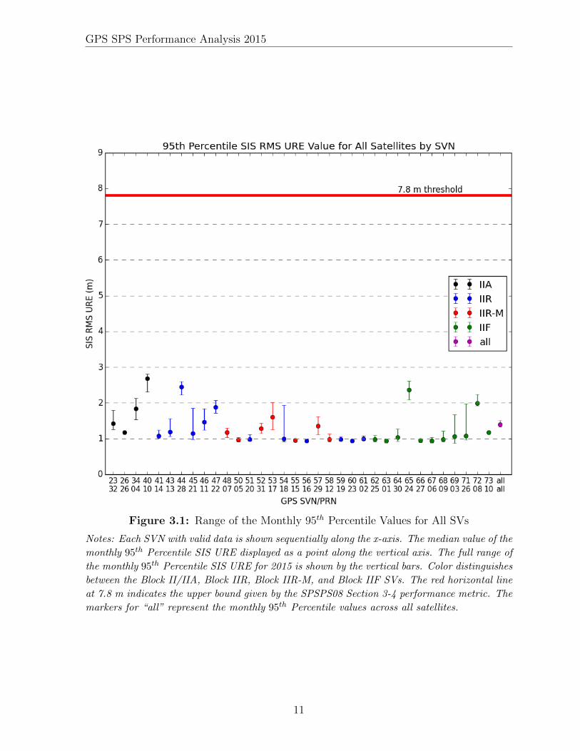
Based on this set of assumptions and constraints, the monthly 95th percentile values ofthe RMS SIS URE were computed for each SV as provided in Table 3.2. Valuescomputed for incomplete months are shown with shaded cells. For each SVN we showthe worst of these values across the year in red. The gaps in URE indicate that thesatellite was decommissioned (SVN 26, 34, 40), or not yet launched (SVN 71, 72, 73).Note that none of the values in this table exceed the threshold of 7.8 m. In all cases, novalues exceed 7.8 m and so this requirement is met for 2015.
Figure 3.1 provides a summary of these results for the entire constellation. For eachSVN, shown along the x-axis, the median value of the monthly 95th percentile SIS UREis computed and displayed as a point. The full range of the annual monthly 95th
percentile SIS URE is shown by the vertical bars. Color distinguishes between theBlock II/IIA, Block IIR, Block IIR-M, and Block IIF SVs. The red horizontal line at7.8 m indicates the upper bound given by the SPSPS08 Section 3-4 performance metric.
A number of points are evident from Figure 3.1:
1. All SVs meet the performance specification of the SPSPS08, even when only theworst performing month is considered. Even the worst value for each SV(indicated by the upper extent of the range bars) is a factor of 2 or more smallerthan the threshold.
2. As a general rule, the newer satellites outperform the older Block IIA satellites interms of the 95th Percentile SIS URE metric. The average performance of theBlock IIA SVs nearly a meter greater than that of the Block IIR, IIR-M, and IIFSVs if SVN 65/PRN 24 and SVN 72/PRN 08 are omitted (see Table 3.2 andpoint 6. below).
3. For most of the SVs, the value of the 95th Percentile SIS URE metric is relativelystable over the course of the year, as indicated by relatively small range bars.
4. For some SVs there are large range extents for the bars. This includes SVNs 45,54, 69, and 71, each of which have spreads of URE values of greater than 1 m. For45, 54, and 69, the maximum value was from a single month of out-of-familiyperformance. For SVN 71, the large value was the first month of operationfollowing launch.
5. The “best” SVs appear to be the Block IIR, Block IIR-M, and Block IIF whichcluster near the 1.0 m level, and whose range variation is small. This includesSVNs 50, 51, 55, 56, 58, 59, 60, 61, 62, 63, 66, and 67.
6. The values for SVN 65 and SVN 72 are noticeably different than the other BlockIIF SVs. These are the only Block IIF SVs operating on a Cesium frequencystandard.
7. Three new SVs were launched in 2015: SVN 71, 72, and 73. The RMS SIS UREvalues for new SVs are sometimes slightly worse for the first few months ofoperation. See the April value for SVN 71 in Table 3.2 for an example.
9

GPS SPS Performance Analysis 2015
Table 3.2: Monthly 95th Percentile Values of SIS RMS URE for All SVs in MetersSVN PRN Block Jan. Feb. Mar. Apr. May Jun. Jul. Aug. Sept. Oct. Nov. Dec. 201523 32 IIA 1.69 1.25 1.42 1.69 1.25 1.30 1.48 1.30 1.80 1.53 1.40 1.39 1.4726 26 IIA 1.17 1.1734 4 IIA 1.80 2.13 2.06 1.67 1.96 1.86 1.77 1.98 1.62 1.53 1.83 1.8540 10 IIA 2.48 2.31 2.46 2.72 2.81 2.77 2.74 2.6441 14 IIR 1.02 1.03 1.24 1.01 1.18 1.04 1.16 1.07 1.11 1.09 1.06 1.00 1.0843 13 IIR 1.19 1.12 1.10 1.28 1.15 1.16 1.26 1.56 1.23 1.19 1.08 1.06 1.2044 28 IIR 2.42 2.30 2.45 2.44 2.22 2.55 2.48 2.59 2.46 2.40 2.50 2.52 2.4545 21 IIR 1.85 1.32 1.26 1.34 1.05 1.14 1.09 1.19 1.10 1.05 0.98 1.02 1.1746 11 IIR 1.24 1.33 1.60 1.29 1.37 1.53 1.30 1.47 1.37 1.81 1.80 1.84 1.5047 22 IIR 1.95 2.02 2.05 1.74 1.80 1.71 1.87 1.76 2.07 1.91 1.91 1.72 1.8848 7 IIR-M 1.18 1.11 1.18 1.12 1.20 1.09 1.12 1.04 1.20 1.30 1.23 1.18 1.1650 5 IIR-M 0.93 0.92 1.04 0.97 0.95 0.96 1.01 1.03 0.95 0.96 0.95 0.94 0.9751 20 IIR 0.93 0.94 0.98 1.12 0.94 1.02 0.99 1.03 0.96 0.96 0.95 0.98 0.9852 31 IIR-M 1.21 1.29 1.15 1.43 1.27 1.21 1.31 1.18 1.39 1.33 1.27 1.40 1.2953 17 IIR-M 1.69 1.59 2.02 1.44 1.60 1.62 1.53 1.33 1.59 1.26 1.79 1.65 1.6054 18 IIR 0.94 0.95 0.95 0.95 0.99 0.94 0.91 1.26 1.93 1.26 1.43 1.57 1.1655 15 IIR-M 0.97 0.92 0.92 0.93 0.91 0.99 0.95 0.93 0.93 0.96 0.96 0.98 0.9556 16 IIR 0.98 0.93 0.95 0.99 0.91 0.91 0.92 0.93 0.92 0.94 0.97 0.93 0.9457 29 IIR-M 1.11 1.36 1.62 1.36 1.43 1.36 1.26 1.49 1.55 1.27 1.39 1.36 1.3758 12 IIR-M 1.06 1.14 0.91 0.94 0.92 1.00 0.99 1.01 0.96 1.01 0.97 0.95 0.9959 19 IIR 0.97 1.06 1.07 1.01 0.96 0.98 0.97 1.03 0.95 0.98 0.96 0.95 0.9860 23 IIR 0.93 0.97 0.96 0.94 0.94 0.97 0.94 0.93 0.92 0.90 0.93 0.96 0.9461 2 IIR 1.00 1.07 0.97 0.95 1.02 1.08 1.04 1.00 0.96 0.97 0.96 0.97 1.0062 25 IIF 0.92 0.92 0.98 1.05 0.97 0.97 0.99 1.03 1.10 0.95 0.97 0.96 0.9963 1 IIF 0.95 0.99 0.95 0.90 0.88 0.92 0.94 0.98 0.96 0.94 0.91 0.92 0.9464 30 IIF 1.18 1.01 0.93 1.28 0.99 1.04 1.09 1.20 0.97 0.97 0.97 1.07 1.0465 24 IIF 2.43 2.44 2.32 2.36 2.61 2.25 2.39 2.35 2.08 2.25 2.36 2.55 2.3966 27 IIF 0.97 0.94 0.89 0.90 0.93 0.97 0.99 0.95 0.94 0.94 0.97 0.96 0.9567 6 IIF 0.97 1.00 0.93 0.89 0.88 0.91 0.97 1.04 0.94 0.95 0.89 0.93 0.9568 9 IIF 0.98 0.92 0.94 0.99 1.06 1.01 0.94 0.92 1.21 0.97 0.99 0.94 0.9969 3 IIF 1.06 1.29 1.67 1.34 1.04 0.87 0.93 0.99 1.01 1.07 1.06 0.95 1.1371 26 IIF 1.98 1.48 1.09 1.07 1.06 1.11 1.01 0.98 0.97 1.1372 8 IIF 1.97 2.00 1.99 1.92 2.24 2.0373 10 IIF 1.17 1.17
Block IIA 2.01 2.04 2.07 2.20 2.37 2.20 1.94 1.66 1.71 1.53 1.48 1.39 2.00Block IIR/IIR-M 1.30 1.27 1.34 1.30 1.27 1.26 1.26 1.25 1.36 1.30 1.31 1.33 1.30
Block IIF 1.24 1.30 1.33 1.47 1.33 1.18 1.16 1.43 1.34 1.39 1.44 1.50 1.35All SVs 1.42 1.41 1.47 1.50 1.43 1.39 1.33 1.35 1.40 1.35 1.36 1.39 1.40
Notes: Values not present indicate that the satellite was unavailable during this period. Monthsduring which an SV was available for less than 25 days are shown shaded. Months with the highestSIS RMS URE for a given SV are colored red. The column labeled “2015” is the 95th Percentileover the year. The four rows at the bottom are the monthly 95th Percentile values over varioussets of SVs.
10
GPS SPS Performance Analysis 2015
Figure 3.1: Range of the Monthly 95th Percentile Values for All SVs
Notes: Each SVN with valid data is shown sequentially along the x-axis. The median value of the
monthly 95th Percentile SIS URE displayed as a point along the vertical axis. The full range of
the monthly 95th Percentile SIS URE for 2015 is shown by the vertical bars. Color distinguishes
between the Block II/IIA, Block IIR, Block IIR-M, and Block IIF SVs. The red horizontal line
at 7.8 m indicates the upper bound given by the SPSPS08 Section 3-4 performance metric. The
markers for “all” represent the monthly 95th Percentile values across all satellites.
11

GPS SPS Performance Analysis 2015
3.1.1.1 An Alternate Approach
As described toward the end of Section 3.1, the 95th percentile Global Average UREvalues are formed by first deriving the Instantaneous RMS SIS URE at a succession oftime points, then picking the 95th percentile value over that set of results. This has thecomputational advantage that the Instantaneous RMS SIS URE is derived from a singleequation in radial, along-track, cross-track, and time errors at a given instant in time(as explained in Appendix B.3). However, it leads to a two-step implementation underwhich we first derive an RMS over a spatial area at a series of time points, then derivea 95th percentile statistic over time.
Given current computation and storage capability, it is practical to derive a set of95th percentile URE values in which the Instantaneous SIS URE values are derived overa reasonably dense grid at a uniform cadence throughout the period of interest. The95th percentile value is then selected from the entire set of Instantaneous SIS UREvalues. This was done in parallel to the process that produced the results shown inSection 3.1.1. A five-degree uniform grid was used along with a 5 minute cadence.Further details on the implementation are provided in Appendix B.4.
Table 3.3 presents a summary of the results obtained by this alternate method. Thistable is in the same format as Table 3.2. Figure 3.2 (which is in the same format asFigure 3.1) presents the values in Table 3.3 in a graphical manner. The values inTable 3.3 are larger than the values in Table 3.2 by an average of 0.02 m. Themaximum difference (alternate - original) for a given SV-month is 0.14 m; the minimumdifference is -0.12 m.
Figure 3.3 is an illustration of the differences between the Monthly 95th percentile SISURE values calculated by the two different methods. Each pair of monthly values for agiven SV found in Table 3.2 and Table 3.3 were taken and the difference computed asthe quantity [alternate - original]. The median, maximum, and minimum differenceswere then selected from each set and plotted in Figure 3.3. (Note: The single monthlyvalue for SVN 26/PRN 26 is based on five days of data prior to decommissioning.)Figure 3.3 illustrates that the two methods agree to within 20 cm and generally a gooddeal less with the alternate method typically being a few cm larger.
None of the values in Table 3.3 exceed the threshold of 7.8 m. Therefore, the thresholdis met for 2015 even under this alternate interpretation of the metric.
3.1.2 URE at Any AOD
The next URE metric considered is the calculation of URE at any AOD. This isassociated with the following SPSPS08 Section 3-4 metrics:
• “≤ 12.8 m 95% Global Average URE during Normal Operations at Any AOD”
This metric may be decomposed in a manner similar to the previous metrics. The keydifference is the term “at any AOD” and the change in the threshold values. The
12

GPS SPS Performance Analysis 2015
Table 3.3: Monthly 95th Percentile Values of SIS Instantaneous URE for all SVs in Meters(via Alternate Method)SVN PRN Block Jan. Feb. Mar. Apr. May Jun. Jul. Aug. Sept. Oct. Nov. Dec. 201523 32 IIA 1.67 1.28 1.45 1.71 1.30 1.30 1.49 1.32 1.85 1.59 1.43 1.40 1.5026 26 IIA 1.05 1.0534 4 IIA 1.88 2.20 2.11 1.71 1.94 1.86 1.81 2.04 1.67 1.53 1.82 1.8840 10 IIA 2.45 2.32 2.50 2.74 2.83 2.77 2.76 2.6541 14 IIR 1.05 1.08 1.30 1.03 1.21 1.05 1.17 1.13 1.13 1.13 1.10 1.01 1.1143 13 IIR 1.20 1.16 1.13 1.31 1.20 1.18 1.27 1.57 1.24 1.21 1.09 1.11 1.2244 28 IIR 2.41 2.31 2.45 2.46 2.25 2.56 2.50 2.59 2.46 2.42 2.51 2.50 2.4645 21 IIR 1.85 1.35 1.30 1.36 1.11 1.16 1.13 1.22 1.13 1.09 1.02 1.07 1.2146 11 IIR 1.26 1.37 1.63 1.31 1.38 1.54 1.33 1.50 1.38 1.81 1.83 1.83 1.5347 22 IIR 1.96 2.02 2.04 1.79 1.85 1.75 1.84 1.76 2.11 1.95 1.89 1.75 1.8948 7 IIR-M 1.20 1.13 1.20 1.14 1.17 1.10 1.15 1.06 1.24 1.29 1.23 1.22 1.1850 5 IIR-M 0.95 0.93 1.04 0.99 0.96 0.98 1.03 1.04 0.98 0.99 0.96 0.97 0.9951 20 IIR 0.95 0.96 1.01 1.14 0.96 1.06 1.03 1.08 0.98 0.99 0.99 1.01 1.0152 31 IIR-M 1.23 1.31 1.18 1.43 1.29 1.26 1.32 1.21 1.43 1.36 1.30 1.43 1.3153 17 IIR-M 1.67 1.60 2.03 1.46 1.65 1.60 1.54 1.36 1.55 1.31 1.78 1.71 1.6154 18 IIR 0.98 0.99 0.98 1.00 1.02 0.96 0.94 1.30 1.90 1.33 1.42 1.61 1.1955 15 IIR-M 0.99 0.95 0.95 0.97 0.96 1.03 0.98 0.97 0.98 0.99 0.99 1.03 0.9856 16 IIR 1.00 0.96 0.97 1.01 0.93 0.93 0.95 0.95 0.94 0.95 0.98 0.96 0.9657 29 IIR-M 1.18 1.48 1.69 1.48 1.50 1.37 1.31 1.52 1.55 1.40 1.45 1.41 1.4358 12 IIR-M 1.11 1.18 0.93 0.97 0.95 1.04 1.04 1.05 1.00 1.03 1.01 0.98 1.0259 19 IIR 1.01 1.07 1.08 1.03 0.98 1.00 0.98 1.04 0.97 1.00 0.97 0.98 1.0160 23 IIR 0.96 1.01 1.00 0.97 0.96 1.01 0.98 0.95 0.95 0.92 0.95 0.99 0.9761 2 IIR 1.02 1.11 1.00 0.97 1.04 1.11 1.07 1.03 0.98 1.00 0.98 1.00 1.0262 25 IIF 0.94 0.95 1.02 1.07 0.99 1.00 1.03 1.06 1.13 0.99 0.99 0.98 1.0263 1 IIF 0.97 1.00 0.97 0.92 0.90 0.95 0.97 0.99 1.00 0.99 0.94 0.94 0.9664 30 IIF 1.14 1.01 0.95 1.27 1.02 1.09 1.13 1.24 0.99 0.99 1.00 1.07 1.0665 24 IIF 2.45 2.45 2.34 2.39 2.62 2.28 2.40 2.36 2.11 2.27 2.38 2.56 2.4066 27 IIF 1.00 0.96 0.91 0.93 0.95 1.00 1.01 0.97 0.96 0.97 0.99 0.99 0.9767 6 IIF 1.00 1.03 0.94 0.90 0.89 0.93 0.99 1.05 0.96 0.97 0.92 0.96 0.9768 9 IIF 0.99 0.94 0.96 1.02 1.08 1.03 0.97 0.93 1.23 1.00 1.01 0.99 1.0169 3 IIF 1.07 1.34 1.64 1.41 1.05 0.89 0.93 1.02 1.03 1.11 1.10 0.97 1.1671 26 IIF 2.03 1.50 1.11 1.11 1.08 1.15 1.03 1.02 0.99 1.1672 8 IIF 2.07 2.02 2.03 1.95 2.25 2.0773 10 IIF 1.24 1.24
Block IIA 2.02 2.07 2.10 2.24 2.37 2.22 1.97 1.69 1.75 1.55 1.48 1.40 2.02Block IIR/IIR-M 1.30 1.29 1.36 1.32 1.28 1.29 1.29 1.29 1.38 1.33 1.34 1.35 1.32
Block IIF 1.24 1.33 1.34 1.47 1.34 1.20 1.20 1.41 1.36 1.40 1.44 1.49 1.36All SVs 1.41 1.43 1.47 1.52 1.44 1.40 1.35 1.36 1.42 1.38 1.38 1.40 1.41
13

GPS SPS Performance Analysis 2015
Figure 3.2: Range of the Monthly 95th Percentile Values for all SVs (via AlternateMethod)
Figure 3.3: Range of Differences in Monthly Values for all SVs
14
GPS SPS Performance Analysis 2015
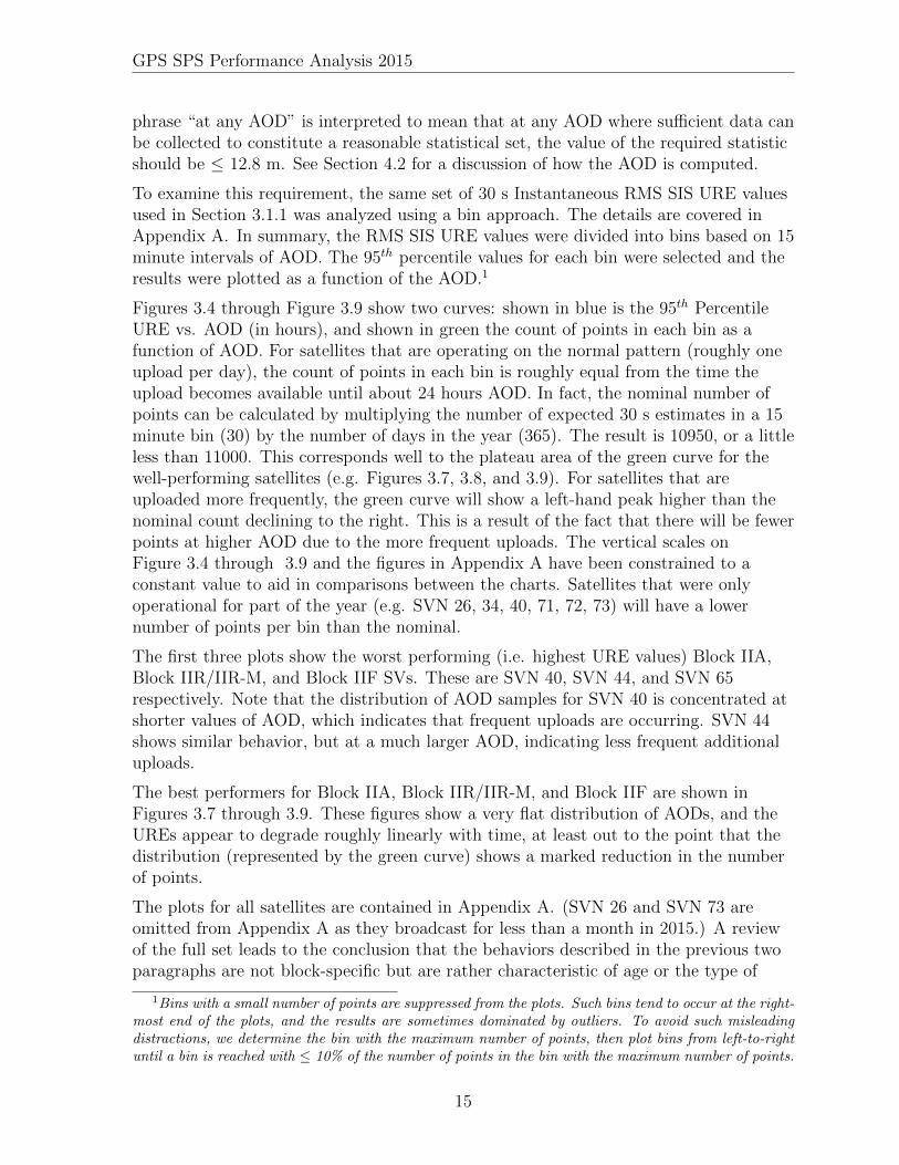
phrase “at any AOD” is interpreted to mean that at any AOD where sufficient data canbe collected to constitute a reasonable statistical set, the value of the required statisticshould be ≤ 12.8 m. See Section 4.2 for a discussion of how the AOD is computed.
To examine this requirement, the same set of 30 s Instantaneous RMS SIS URE valuesused in Section 3.1.1 was analyzed using a bin approach. The details are covered inAppendix A. In summary, the RMS SIS URE values were divided into bins based on 15minute intervals of AOD. The 95th percentile values for each bin were selected and theresults were plotted as a function of the AOD.1
Figures 3.4 through Figure 3.9 show two curves: shown in blue is the 95th PercentileURE vs. AOD (in hours), and shown in green the count of points in each bin as afunction of AOD. For satellites that are operating on the normal pattern (roughly oneupload per day), the count of points in each bin is roughly equal from the time theupload becomes available until about 24 hours AOD. In fact, the nominal number ofpoints can be calculated by multiplying the number of expected 30 s estimates in a 15minute bin (30) by the number of days in the year (365). The result is 10950, or a littleless than 11000. This corresponds well to the plateau area of the green curve for thewell-performing satellites (e.g. Figures 3.7, 3.8, and 3.9). For satellites that areuploaded more frequently, the green curve will show a left-hand peak higher than thenominal count declining to the right. This is a result of the fact that there will be fewerpoints at higher AOD due to the more frequent uploads. The vertical scales onFigure 3.4 through 3.9 and the figures in Appendix A have been constrained to aconstant value to aid in comparisons between the charts. Satellites that were onlyoperational for part of the year (e.g. SVN 26, 34, 40, 71, 72, 73) will have a lowernumber of points per bin than the nominal.
The first three plots show the worst performing (i.e. highest URE values) Block IIA,Block IIR/IIR-M, and Block IIF SVs. These are SVN 40, SVN 44, and SVN 65respectively. Note that the distribution of AOD samples for SVN 40 is concentrated atshorter values of AOD, which indicates that frequent uploads are occurring. SVN 44shows similar behavior, but at a much larger AOD, indicating less frequent additionaluploads.
The best performers for Block IIA, Block IIR/IIR-M, and Block IIF are shown inFigures 3.7 through 3.9. These figures show a very flat distribution of AODs, and theUREs appear to degrade roughly linearly with time, at least out to the point that thedistribution (represented by the green curve) shows a marked reduction in the numberof points.
The plots for all satellites are contained in Appendix A. (SVN 26 and SVN 73 areomitted from Appendix A as they broadcast for less than a month in 2015.) A reviewof the full set leads to the conclusion that the behaviors described in the previous twoparagraphs are not block-specific but are rather characteristic of age or the type of
1Bins with a small number of points are suppressed from the plots. Such bins tend to occur at the right-most end of the plots, and the results are sometimes dominated by outliers. To avoid such misleadingdistractions, we determine the bin with the maximum number of points, then plot bins from left-to-rightuntil a bin is reached with ≤ 10% of the number of points in the bin with the maximum number of points.
15

GPS SPS Performance Analysis 2015
frequency standard. For example, two of the three Block IIA satellites exhibit evidenceof more frequent uploads as indicated by an uneven distribution of observation acrossthe time bins. Among the Block IIF SVs, the rate of URE growth is noticeably higherfor the two satellites that use a Cesium frequency standard. While there are noticeabledifferences between individual satellites, all the results are well within the assertion forthis metric.
16

GPS SPS Performance Analysis 2015
0 5 10 15 20 25 30Age of Data (hours)
0
1
2
3
4
5
SPS
SIS
RM
S UR
E (m
)
0
2000
4000
6000
8000
10000
12000
14000
16000
18000
Num
ber o
f Poi
nts
95th Percentile SIS RMS URE Values by AOD for SVN40/PRN10, 2015SPS SIS URE Value Num Points
Figure 3.4: Worst Performing Block IIA SV in Terms of Any AOD (SVN 40/PRN 10)
0 5 10 15 20 25 30Age of Data (hours)
0
1
2
3
4
5
SPS
SIS
RM
S UR
E (m
)
0
2000
4000
6000
8000
10000
12000
14000
16000
18000
Num
ber o
f Poi
nts
95th Percentile SIS RMS URE Values by AOD for SVN44/PRN28, 2015SPS SIS URE Value Num Points
Figure 3.5: Worst Performing Block IIR/IIR-M SV in Terms of Any AOD (SVN44/PRN 28)
17

GPS SPS Performance Analysis 2015
0 5 10 15 20 25 30Age of Data (hours)
0
1
2
3
4
5
SPS
SIS
RM
S UR
E (m
)
0
2000
4000
6000
8000
10000
12000
14000
16000
18000
Num
ber o
f Poi
nts
95th Percentile SIS RMS URE Values by AOD for SVN65/PRN24, 2015SPS SIS URE Value Num Points
Figure 3.6: Worst Performing Block IIF SV in Terms of Any AOD (SVN 65/PRN 24)
0 5 10 15 20 25 30Age of Data (hours)
0
1
2
3
4
5
SPS
SIS
RM
S UR
E (m
)
0
2000
4000
6000
8000
10000
12000
14000
16000
18000
Num
ber o
f Poi
nts
95th Percentile SIS RMS URE Values by AOD for SVN23/PRN32, 2015SPS SIS URE Value Num Points
Figure 3.7: Best Performing Block IIA SV in Terms of Any AOD (SVN 23/PRN 32)
18

GPS SPS Performance Analysis 2015
0 5 10 15 20 25 30Age of Data (hours)
0
1
2
3
4
5
SPS
SIS
RM
S UR
E (m
)
0
2000
4000
6000
8000
10000
12000
14000
16000
18000
Num
ber o
f Poi
nts
95th Percentile SIS RMS URE Values by AOD for SVN60/PRN23, 2015SPS SIS URE Value Num Points
Figure 3.8: Best Performing Block IIR/IIR-M SV in Terms of Any AOD (SVN 60/PRN23)
0 5 10 15 20 25 30Age of Data (hours)
0
1
2
3
4
5
SPS
SIS
RM
S UR
E (m
)
0
2000
4000
6000
8000
10000
12000
14000
16000
18000
Num
ber o
f Poi
nts
95th Percentile SIS RMS URE Values by AOD for SVN63/PRN01, 2015SPS SIS URE Value Num Points
Figure 3.9: Best Performing Block IIF SV in Terms of Any AOD (SVN 63/PRN 01)
19

GPS SPS Performance Analysis 2015
3.1.3 URE at Zero AOD
Another URE metric considered is the calculation of URE at Zero Age of Data(ZAOD). This is associated with the SPSPS08 Section 3-4 metric:
• “≤ 6.0 m 95% Global Average URE during Normal Operations at Zero AOD”
This metric may be decomposed in a manner similar to the previous two metrics. Thekey difference is the term “at Zero AOD” and the change in the threshold values.
The broadcast ephemeris is never available to user equipment at ZAOD simply due tothe delays inherent in preparing the broadcast ephemeris and uploading it to the SV.However, we can still make a case that this assertion is met by examining the 95th
percentile SIS RMS URE value at 15 minutes AOD. These values are represented bythe left-most data point on the red lines shown in Figure 3.4 through Figure 3.9. TheZAOD values should be slightly better than the 15 minute AOD values, or at worstroughly comparable. Inspection of the 15 minute AOD values shows that the values forall SVs are well within the 6.0 m value associated with the assertion. Therefore theassertion is fulfilled.
3.1.4 URE Bounding
The SPSPS08 asserts the following requirements for single-frequency C/A code:
• “≤ 30 m 99.94% Global Average URE during Normal Operations”
• “≤ 30 m 99.79% Worst Case Single Point Average URE during NormalOperations”
As noted earlier the 30 s instantaneous SIS RMS URE values were used to evaluatethese requirements. However, there are limitations to our technique of estimating UREsthat are worth noting such as fits across orbit/clock discontinuities, thrust events, andclock run-offs. These are discussed in Appendix B.5. As a result of these limitations,the UREs were used only as a screening tool to identify possible violations of thisrequirement. Possible candidate events were then screened further by examining theobserved range deviations (ORDs) to determine actual values during the event.
The ORDs are formed using the observation data collected to support the positionaccuracy analysis described in Section 3.5.4. In the case of ORDs, the observed range isdifferenced from the range predicted by subtracting the known station position fromthe SV location derived from the broadcast ephemeris. The selected stations aregeographically distributed such that at least two sets of observations are available foreach SV at all times. As a result, any actual SV problems that would lead to aviolation of this assertion will produce large ORDs from multiple stations.
The 30 s instantaneous SIS RMS URE values and the 30 s ORD values throughout2015 were examined to determine if any values exceeded 30 m. No such values werefound. As a result, these assertions are considered satisfied.
20

GPS SPS Performance Analysis 2015
3.1.5 UTC Offset Error Accuracy
The SPS PS provides the following assertion regarding SPS PS UTC offset error(UTCOE) Accuracy:
• “≤ 40 nsec 95% Global Average UTCOE during Normal Operations at Any AOD”
The conditions and constraints state that this assertion should be true for any healthySPS SIS.
This assertion was evaluated by calculating the global average UTCOE at each 15minute interval. The GPS-UTC offset available to the user was calculated based on theGPS broadcast navigation message data available from the SV at that time. TheGPS-UTC offset truth information was provided by the USNO daily GPS-UTC offsetvalues. A multi-day spline was fit to the daily truth values and the USNO value forGPS-UTC at each evaluation epoch was derived from this fit.
The selection and averaging algorithms are a key part of this process. The globalaverage at each 15 minute epoch is determined by evaluating the UTCOE at each pointon a 111 km × 111 km grid across the entire surface of the earth. (This grid spacingcorresponds to roughly one degree at the Equator.) At each grid point, the algorithmdetermines the set of SVs visible at-or-above the 5◦ minimum elevation angle that arebroadcasting a healthy indication in the navigation message. For each of these SVs, theUTC offset information in page 18, subframe 4 are compared in order to determine thedata set that has an epoch time (tot) that is the latest of those that fall in the range(current time) ≤ tot ≤ (current time+ 72 hours). These data are used to form theUTC offset and UTCOE for that time-grid point.
The global averages at each evaluation epoch are assembled into monthly data sets.The 95th percentile values are then selected from these sets.
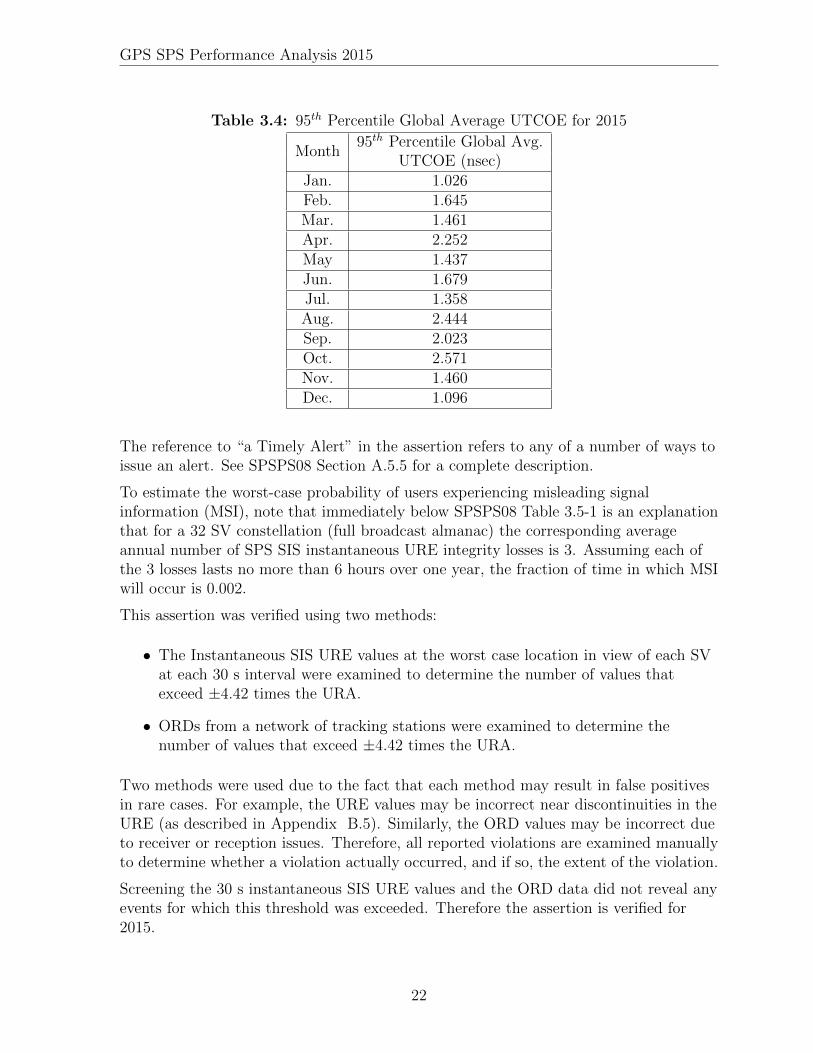
Table 3.4 provides the results for each month of 2015. None of these values exceed theassertion of 40 nsec. Therefore the assertion is verified for 2015.
3.2 SIS Integrity
3.2.1 URE Integrity
Under the heading of SIS Integrity, the SPSPS08 makes the following assertion inSection 3.5.1, Table 3.5-1:
• “≤ 1 × 10⁻⁵ Probability Over Any Hour of the SPS SIS Instantaneous UREExceeding the NTE Tolerance Without a Timely Alert During Normal Operations”
The associated conditions and constraints include a limitation to healthy SIS, a Not toExceed (NTE) tolerance ±4.42 times the upper bound on the user range accuracy(URA) currently broadcast, and a worst case for a delayed alert of 6 hours.
21
GPS SPS Performance Analysis 2015
Table 3.4: 95th Percentile Global Average UTCOE for 2015
Month95th Percentile Global Avg.
UTCOE (nsec)Jan. 1.026Feb. 1.645Mar. 1.461Apr. 2.252May 1.437Jun. 1.679Jul. 1.358Aug. 2.444Sep. 2.023Oct. 2.571Nov. 1.460Dec. 1.096
The reference to “a Timely Alert” in the assertion refers to any of a number of ways toissue an alert. See SPSPS08 Section A.5.5 for a complete description.
To estimate the worst-case probability of users experiencing misleading signalinformation (MSI), note that immediately below SPSPS08 Table 3.5-1 is an explanationthat for a 32 SV constellation (full broadcast almanac) the corresponding averageannual number of SPS SIS instantaneous URE integrity losses is 3. Assuming each ofthe 3 losses lasts no more than 6 hours over one year, the fraction of time in which MSIwill occur is 0.002.
This assertion was verified using two methods:
• The Instantaneous SIS URE values at the worst case location in view of each SVat each 30 s interval were examined to determine the number of values thatexceed ±4.42 times the URA.
• ORDs from a network of tracking stations were examined to determine thenumber of values that exceed ±4.42 times the URA.
Two methods were used due to the fact that each method may result in false positivesin rare cases. For example, the URE values may be incorrect near discontinuities in theURE (as described in Appendix B.5). Similarly, the ORD values may be incorrect dueto receiver or reception issues. Therefore, all reported violations are examined manuallyto determine whether a violation actually occurred, and if so, the extent of the violation.
Screening the 30 s instantaneous SIS URE values and the ORD data did not reveal anyevents for which this threshold was exceeded. Therefore the assertion is verified for2015.
22

GPS SPS Performance Analysis 2015
3.2.2 UTCOE Integrity
The SPS PS provides the following assertion regarding SPS PS UTCOE Integrity inSection 3.5.4:
• “≤ 1 × 10⁻⁵ Probability Over Any Hour of the SPS SIS Instantaneous UTCOEExceeding the NTE Tolerance Without A Timely Alert during Normal Operations”
The associated conditions and constraints include a limitation to healthy SIS, a NTEtolerance of ±120 nsec, and the note that this holds true for any healthy SPS SIS. Thereference to “a Timely Alert” in the assertion refers to any of a number of ways to issuean alert. See SPSPS08 Section A.5.5 for a complete description.
This assertion was evaluated by calculating the UTC offset for the page 18, subframe 4data broadcast by each SV transmitting a healthy indication in the navigation messageat each 15 minute interval. That offset was used to compute the corresponding UTCOEfrom truth data obtained from the USNO. Any UTCOE values that exceed the NTEthreshold of ±120 nsec were investigated to determine if they represent actualviolations of the NTE threshold or were artifacts of data processing.
No values exceeding the NTE threshold were found in 2015. The value farthest fromzero for the year was -4.5 nsec (during August). Therefore the assertion is verified for2015.
3.3 SIS Continuity
3.3.1 Unscheduled Failure Interruptions
The metric is stated in SPSPS08 Table 3.6-1 as follows:
• “≥ 0.9998 Probability Over Any Hour of Not Losing the SPS SIS Availabilityfrom a Slot Due to Unscheduled Interruption”
The conditions and constraints note the following:
• The empirical estimate of the probability is calculated as an average over all slotsin the 24-slot constellation, normalized annually.
• The SPS SIS is available from the slot at the start of the hour.
The notion of SIS continuity is slightly more complex for an expandable slot, becausemultiple SVs are involved. Following SPSPS08 Section A.6.5, a loss of continuity isconsidered to occur when,
23

GPS SPS Performance Analysis 2015
“The expandable slot is in the expanded configuration, and either one of thepair of satellites occupying the orbital locations defined in Table 3.2-2 for theslot loses continuity.”
Hence, the continuity of signal of the expanded slot will be determined by whethereither SV loses continuity.
Another point is that there is some ambiguity in this metric, which is stated in terms of“a slot” while the associated Conditions and Constraints note that this is an averageover all slots. Therefore both the per-slot and 24-slot constellation averages have beencomputed. As discussed below, while the per-slot values are interesting, theconstellation average is the correct value to compare to the SPS PS metric.
Three factors must be considered in looking at this metric:
1. We must establish which SVs were assigned to which slots during the period ofthe evaluation.
2. We must determine when SVs were not transmitting (or not transmitting a PRNavailable to users).
3. We must determine which interruptions were scheduled vs. unscheduled.
The derivation of the SV/Slot assignments is described in Appendix E.
For purposes of this report, interruptions were considered to have occurred if one ormore of the SV(s) assigned to the given slot is (are) unhealthy in the sense of SPSPS08Section 2.3.2. The following specific indications were considered:
• If the health bits in navigation message subframe 1 are set to anything other thanall zeros.
• If an appropriately distributed worldwide network of stations failed to collect anypseudorange data sets for a given measurement interval.
The latter case (failure to collect any data) indicates that the satellite signal wasremoved from service (e.g. non-standard code or some other means). The NGA MSNprovides at least two-station visiblity (and at least 90% three-station visibility) withredundant receivers at each station, both continuously monitoring up to 12 SVs inview. Therefore, if no data for a satellite are received for a specific time, it is highlylikely that the satellite was not transmitting on the assigned PRN at that time. The 30s Receiver Independent Exchange format (RINEX) [6] observation files from thisnetwork were examined for each measurement interval (i.e. every 30 s) for each SV. Ifat least one receiver collected a pseudorange data set on L1 C/A, L1 P(Y), and L2P(Y) with a signal-to-noise level of at least 25 dB-Hz on all frequencies and noloss-of-lock flags, the SV is considered trackable at that moment. In addition, the 30 sIGS data collected to support the position accuracy estimates (Section 3.5.4) were
24
GPS SPS Performance Analysis 2015
examined in a similar fashion to guard against any MSN control center outages thatcould have led to missing data across multiple stations simultaneously. This allows usto define an epoch-by-epoch availability for each satellite. Then, for each slot, eachhour in year was examined, and if any SV occupying the slot was not available at thestart of the hour, the hour was not considered as part of the evaluation of the metric. Ifthe slot was determined to be available, then the remaining data was examined todetermine if an outage occurred during the hour.
The preceding criteria were applied to determine the times and durations ofinterruptions. After this was done, the Notice Advisories to Navstar Users (NANUs)effective in 2015 were reviewed to determine which of these interruptions could beconsidered scheduled interruptions as defined in SPSPS08 Section 3.6. The scheduledinterruptions were removed from consideration for purposes of assessing continuity ofsevice. When a slot was available at the start of an hour but a scheduled interruptionoccurred during the hour, the hour was assessed based on whether data were availableprior to the scheduled outage.
Unscheduled interruptions are not always documented with a NANU. A small numberof short-duration outages not covered by NANUs were observed. When such outagesoccurred on satellites that are assigned to one of 24 slots, the outage was counted inevaluating this assertion.
Scheduled interruptions as defined in the ICD-GPS-240 [7] have a nominal notificationtime of 96 hours prior to the outage. Following the SPSPS08 Section 2.3.5, scheduledinterruptions announced 48 hours in advance are not to be considered as contributing tothe loss of continuity. So to contribute to a loss of continuity, the notification time for ascheduled interruption must occur less than 48 hours in advance of the interruption. Inthe case of an interruption not announced in a timely manner, the time from the startof the interruption to the moment 48 hours after notification time can be considered asa potential unscheduled interruption (for continuity purposes). However, a healthy SISmust exist at the start of any hour for an interruption to be considered to occur.
The following NANU types are considered to represent (or modify) scheduledinterruptions (assuming the 48-hour advance notice is met):
• FCSTDV - Forecast Delta-V
• FCSTMX - Forecast Maintenance
• FCSTEXTD - Forecast Extension
• FCSTRESCD - Forecast Rescheduled
• FCSTUUFN - Forecast Unusable Until Further Notice
The FCSTSUMM (Forecast Summary) NANU that occurs after the outage isreferenced to confirm the actual beginning and ending time of the outage.
For scheduled interruptions that extend beyond the period covered by a FCSTDV orFCSTMX NANU, the uncovered portion will be considered an unscheduled
25

GPS SPS Performance Analysis 2015
interruption. However, if a FCSTEXTD NANU extending the length of a scheduledinterruption is published 48 hours in advance of the effective time of extension, theinterruption will remain categorized as scheduled. It is worth reiterating that, for thecomputation of the metric, only those hours for which a valid SIS is available from theslot at the start of the hour are actually considered in the computation of the values.
Table 3.5 is a summary of the results of the assessment of SIS continuity. Interpretingthe metric as being averaged over the constellation, the constellation exceeded the goalof 0.9998 probability of not losing the SPS SIS availability due to a unscheduledinterruption.
Table 3.5: Probability Over Any Hour of Not Losing Availability Due to UnscheduledInterruption
Plane-Slot # of Hours with the SPS SISavailable at the start of the
hourb
# of Hours withUnscheduledInterruptionc
Fraction of Hours in WhichAvailability was Not Lost
A1 8760 0 1.00000A2 8760 1 0.99989A3 8760 0 1.00000A4 8760 0 1.00000B1a 6122 0 1.00000B2 8760 0 1.00000B3 8760 0 1.00000B4 8760 0 1.00000C1 8760 0 1.00000C2 8760 1 0.99989C3 8760 0 1.00000C4 8760 0 1.00000D1 8760 0 1.00000D2a 8726 2 0.99977D3 8760 0 1.00000D4 8760 0 1.00000E1 8760 0 1.00000E2 8760 0 1.00000E3 8760 0 1.00000E4 8760 0 1.00000F1 8760 0 1.00000F2a 8760 1 0.99989F3 8760 0 1.00000F4 8740 1 0.99989
All Slots 207548 6 0.99997
aWhen B1, D2, and F2 are configured as expandable slots, both slot locations must be occupied by anavailable satellite for the slot to be counted as available.
bThere are 8760 hours in 2015.cNumber of hours in which SPS SIS was available at the start of the hour and during the hour either
(1.) an SV transmitted navigation message with subframe 1 health bits set to other than all zeroes withouta scheduled outage, (2.) signal lost without a scheduled outage, or (3.) the URE NTE tolerance wasviolated.
26
GPS SPS Performance Analysis 2015
To put this in perspective, there were 8760 hours in 2015. The required probability ofnot losing SPS SIS availability implies that there be less than8760× (1− 0.9998) = 1.75 hours that experience unscheduled interruptions in a year. Ifthis were a per-slot metric, this would mean no slot may experience more than oneunscheduled interruption in a year. The maximum number of unscheduled interruptionsover the 24 slot constellation is given by 8760× 24× (1− 0.9998) = 42 unscheduledhours that experience interruptions. This is less than two unscheduled interruptions perSV per year but allows for the possibility that some SVs may have no unscheduledinterruptions while others may have more than one.
Slot B1 is considered empty at the beginning of 2015. The slot has been configured asan expanded slot for some time. (See Appendix E for more on sources of plane-slotinformation.) However, on 28 March 2013 the satellite occupying the B1F half of slotB1 experienced an unscheduled interruption (SVN 35/PRN 30, see NANU 2013022). Itwas later decommissioned (NANU 2013027). B1F remained empty until 20 April 2015when SVN 70/PRN 26 was set initially usuable (NANU 2015028). As a result, forpurposes of this analysis, slot B1 is considered empty for several weeks at the beginningof 2015. In Table 3.5, the row associated with B1 shows a lower number of hours ofavailability than all other rows. While there are multiple unscheduled interruptions inslot B1 during 2015, the unavailable period at the beginning of the year is not countedas it was counted at the beginning of the interruption in 2013. This outage is alsoaddressed in Section 3.4 in terms of the impact on availability.
Returning to Table 3.5, across the constellation slots the total number of hours lost was6. This is smaller than the maximum number of hours of unscheduled interruptions(42) available to meet the metric (see the previous paragraph) and leads to empiricalvalue for the fraction of hours in which SIS continuity was maintained of 0.99997.Therefore, this assertion is considered fulfilled in 2015.
3.3.2 Status and Problem Reporting Standards
3.3.2.1 Scheduled Events
The SPSPS08 makes the following assertion in Section 3.6.3 regarding notification ofscheduled events affecting service:
• “Appropriate NANU issued to Coast Guard and the FAA at least 48 hours priorto the event”
While beyond the assertion in the performance standards, ICD-GPS-240 [7] states anominal notification time of 96 hours prior to outage start and an objective of 7 daysprior to outage start.
This metric was evaluated by examining the NANUs provided throughout the year andcomparing the NANU periods to outages observed in the data. In general, scheduledevents are described in a pair of NANUs. The first NANU is a forecast of when the
27

GPS SPS Performance Analysis 2015
outage will occur. The second NANU is provided after the outage and summarizes theactual start and end times of the outage. (This is described in ICD-GPS-240 Section10.1.1.)
Table 3.6 summarizes the pairs found for 2015. The two leftmost columns provide theSVN/PRN of the subject SV. The next three columns specify the NANU #, type, anddate/time of the NANU for the forecast NANU. These are followed by three columnsthat specify the NANU #, the date/time of the NANU for the FCSTSUMM NANUprovided after the outage, and the date/time of the beginning of the outage. The finalcolumn is the time difference between the time the forecast NANU was released and thebeginning of the actual outage (in hours). This represents the length of time betweenthe release of the forecast and the actual start of the outage.
Table 3.6: Scheduled Events Covered in NANUs for 2015
SVN PRNPrediction NANU Summary NANU (FCSTSUMM) Notice
NANU # TYPE Release Time NANU # Release Time Start Of Outage (hrs)43 13 2015001 FCSTDV 02 Jan 1648Z 2015006 09 Jan 1340Z 09 Jan 0544Z 156.9364 30 2015008 FCSTDV 30 Jan 2008Z 2015009 06 Feb 0558Z 06 Feb 0112Z 149.0741 14 2015013 FCSTDV 27 Feb 1807Z 2015014 05 Mar 2128Z 05 Mar 1512Z 141.0857 29 2015015 FCSTDV 07 Mar 0000Z 2015016 12 Mar 1054Z 12 Mar 0431Z 124.5223 32 2015017 FCSTDV 13 Mar 1854Z 2015018 20 Mar 1530Z 20 Mar 0906Z 158.2023 32 2015020 FCSTMX 26 Mar 2110Z 2015023 31 Mar 2335Z 30 Mar 0005Z 74.9256 16 2015024 FCSTDV 09 Apr 2231Z 2015025 15 Apr 2134Z 15 Apr 1608Z 137.6250 05 2015026 FCSTDV 17 Apr 1618Z 2015029 22 Apr 0352Z 21 Apr 2129Z 101.1854 18 2015031 FCSTDV 24 Apr 1901Z 2015033 01 May 0552Z 01 May 0031Z 149.5061 02 2015034 FCSTDV 05 May 2207Z 2015035 13 May 0150Z 12 May 1809Z 164.0368 09 2015038 FCSTDV 19 May 2042Z 2015040 28 May 1922Z 28 May 1400Z 209.3045 21 2015041 FCSTDV 29 May 1507Z 2015045 05 Jun 0902Z 05 Jun 0327Z 156.3352 31 2015044 FCSTDV 04 Jun 2050Z 2015047 11 Jun 1505Z 11 Jun 0952Z 157.0362 25 2015043 FCSTMX 04 Jun 1954Z 2015048 11 Jun 1814Z 11 Jun 1452Z 162.9766 27 2015046 FCSTMX 10 Jun 1515Z 2015051 15 Jun 1657Z 15 Jun 1332Z 118.2865 24 2015049 FCSTMX 12 Jun 1531Z 2015055 17 Jun 1451Z 17 Jun 1129Z 115.9771 26 2015050 FCSTMX 12 Jun 1550Z 2015056 19 Jun 0351Z 19 Jun 0047Z 152.9567 06 2015052 FCSTMX 16 Jun 1545Z 2015058 24 Jun 0121Z 23 Jun 2054Z 173.1564 30 2015053 FCSTMX 16 Jun 1551Z 2015061 25 Jun 2043Z 25 Jun 1658Z 217.1251 20 2015054 FCSTDV 16 Jun 1556Z 2015062 26 Jun 0846Z 26 Jun 0240Z 226.7369 03 2015059 FCSTMX 24 Jun 1929Z 2015063 30 Jun 2237Z 30 Jun 1812Z 142.7268 09 2015060 FCSTMX 24 Jun 2012Z 2015064 01 Jul 2232Z 01 Jul 1951Z 167.6534 04 2015065 FCSTMX 02 Jul 1435Z 2015067 09 Jul 0621Z 09 Jul 0317Z 156.7053 17 2015070 FCSTDV 21 Jul 1929Z 2015071 28 Jul 2144Z 28 Jul 1624Z 164.9259 19 2015072 FCSTDV 07 Aug 1617Z 2015074 13 Aug 1057Z 13 Aug 0319Z 131.0346 11 2015075 FCSTDV 19 Aug 1724Z 2015076 25 Aug 1942Z 25 Aug 1256Z 139.5367 06 2015077 FCSTDV 26 Aug 1915Z 2015078 02 Sep 0058Z 01 Sep 1859Z 143.7360 23 2015079 FCSTDV 03 Sep 2006Z 2015081 11 Sep 1003Z 11 Sep 0330Z 175.4047 22 2015092 FCSTDV 03 Dec 1724Z 2015097 11 Dec 0025Z 10 Dec 1636Z 167.2047 22 2015096 FCSTMX 10 Dec 2104Z 2015099 17 Dec 2041Z 15 Dec 2347Z 122.7269 03 2015098 FCSTDV 11 Dec 1655Z 2015100 18 Dec 0135Z 17 Dec 2025Z 147.5
Average Notice Period 151.81
To meet the assertion in the performance standard, the number of hours in therightmost column of Table 3.6 should always be greater than 48.0. The average noticewas over 151 hours. The shortest notice was 75 hours. Therefore, the assertion hasbeen met.
28

GPS SPS Performance Analysis 2015
Satellites were decommissioned three times in 2015. These were handled as specialcases of scheduled outages. A FCSTUUFN (Forecast unusable until further notice)NANU was provided specifying when the satellite would be set unusable. Followingthis, a DECOM (decommission) NANU was provided following the actual event. Thedetails on the notice provided by these four pairs are provided in Table 3.7. Each of thepairs meets the assertion of the SPS PS and the nominal time of the ICD-GPS-240 forscheduled events.
Table 3.7: Decommissioning Events Covered in NANUs for 2015
SVN PRNFCSTUUFN NANU DECOM NANU Notice
NANU # Release Time NANU # Release Time End of Unusable Period (hrs)26 26 2015002 02 Jan 1659Z 2015005 06 Jan 2219Z 05 Jan 1750Z 72.8540 10 2015066 07 Jul 1852Z 2015069 16 Jul 2217Z 16 Jul 1624Z 213.5334 04 2015089 28 Oct 2019Z 2015091 03 Nov 2216Z 02 Nov 2222Z 122.05
Average Notice Period 136.03
3.3.2.2 Unscheduled Outages
The SPS PS provides the following assertion in Section 3.6.3 regarding notification ofunscheduled outages or problems affecting service:
• “Appropriate NANU issued to Coast Guard and the FAA as soon as possible afterthe event”
The ICD-GPS-240 states that the nominal notification times is less than 1 hour afterthe start of the outage with an objective of 15 minutes.
This metric was evaluated by examining the NANUs provided throughout the year andcomparing the NANU periods to outages observed in the data. Unscheduled eventsmay be covered by either a single NANU or a pair of NANUs. In the case of a briefoutage, a NANU with type UNUNOREF (unusable with no reference) is provided todetail the period of the outage. In the case of longer outages, a UNUSUFN (unusableuntil further notice) is provided to inform users of an ongoing outage or problem. Thisis followed by a NANU with type UNUSABLE after the outage is resolved. (This isdescribed in detail in ICD-GPS-240 Section 10.1.2.)
Table 3.8 provides a list of the unscheduled outages found in the NANU information for2015. The two leftmost columns provide the SVN/PRN of the subject SV. The nexttwo columns provide the NANU #, and date/time of the UNUSUFN NANU. These arefollowed by three columns that specify the NANU #, the date/time of the NANU forthe UNUSABLE NANU provided after the outage, and the date/time of the beginningof the outage. The final column is the time difference between the time the outagebegan and the time the UNUSUFN NANU was released (in minutes). For theUNUNOREF NANUs, only the last four columns are used.
29

GPS SPS Performance Analysis 2015
Table 3.8: Unscheduled Events Covered in NANUs for 2015
SVN PRNUNUSUFN NANU UNUSABLE/UNUNOREF NANU Lag Time
NANU # Release Time NANU # Release Time Start Of Event (minutes)46 11 2015011 19 Feb 0631Z 2015012 20 Feb 1444Z 19 Feb 0450Z 101.0034 04 2015036 19 May 1241Z 2015037 19 May 1454Z 19 May 1246Z -5.0041 14 2015082 08 Oct 1510Z 2015083 08 Oct 1523Z 08 Oct 1500Z 10.0060 23 2015085 19 Oct 1853Z 2015086 20 Oct 1437Z 19 Oct 1800Z 53.0063 01 2015094 09 Dec 1125Z 2015095 09 Dec 1305Z 09 Dec 1003Z 82.0066 27 2015042 03 Jun 1510Z 03 Jun 0603Z 547.0052 31 2015057 22 Jun 1936Z 22 Jun 1919Z 17.00
Average Lag Time 115.00
Because the performance standard states only “as soon as possible after the event”,there is no evaluation to be performed. However, the data are provided for information.With respect to the nominal notification times provided in ICD-GPS-240, it appearsthat the nominal times are typically met (five of seven cases in 2015), but there areexceptions.
3.3.2.3 Suspect NANUs
We noticed three suspect NANUs in 2015.
NANU 2015021: This is a NANU of type GENERAL that announced thedecommissioning of SVN 38. It is suspect in two ways.
• A decommissioning event should be announced in a DECOM NANU and not in aGENERAL NANU.
• SVN 38 was already decommissioned on 30 Oct 2014. The announcement wasprovided in NANU 2014083. Both NANUs agree that SVN 38 was unusable as of30 Oct 2014. However, NANU 2014083 states SVN 38 was removed from theconstellation on 30 Oct 2014 while NANU 2015021 states SVN 38 was removed on26 Mar 2015. It is worth noting that SVN 38 was transmitting for a period inearly 2015 (see NANU 2015003) but remained unusable throughout (as in atypical test of a spare SV). Because SVN 38 was not usable in 2015, we regardNANU 2014083 as correct and NANU 2015021 as being provided in error.
NANU 2015022: This NANU is of type UNUSABLE and references the previousNANU 2015020 which is of type FCSTMX. NANU 2015020 is later appropriately closedby NANU 2015023 which is of the expected type of FCSTSUMM. We assume NANU2015022 was released in error and have ignored it.
NANU 2015082: This NANU is an UNUSUFN but contains no information regardingthe start time of the event. NANU 2015083 was issued 13 minutes after NANU2015082, and contains identical start and end times. NANU 2015084 is a GENERALNANU that explains NANU 2015082 was sent in error with NANU 2015083 followingto close out NANU 2015082.
30

GPS SPS Performance Analysis 2015
3.4 SIS Availability
3.4.1 Per-slot Availability
The SPSPS08 Section 3.7.1 makes two linked statements in this area:
• “≥ 0.957 Probability that a Slot in the Baseline Configuration will be Occupied bya Healthy Navstar Satellite Broadcasting a Useable SPS SIS”
• “≥ 0.957 Probability that a Slot in the Expanded Configuration will be Occupiedby a pair of Healthy Navstar Satellites Each Broadcasting a Useable SPS SIS”
The constraints include the note that this is to be calculated as an average over all slotsin the 24-slot constellation, normalized annually.
The derivation of the SV/Slot assignments is described in Appendix E.
This metric was verified by examining the status of each SV in the Baseline 24- Slotconfiguration (or pair of SVs in an Expandable Slot) at every 30 s interval throughoutthe year. The health status was determined from the subframe 1 health bits of theephemeris being broadcast at the time of interest. In addition, data from monitorstation networks were examined to verify that the SV was broadcasting a trackablesignal at the time. The results are summarized in Table 3.9.
Slot B1 presented an unusual situation in 2015. Slot B1 has been configured as anexpanded slot for some time. (See Appendix E for more on sources of plane-slotinformation.) However, the B1F half of slot B1 was unoccupied from the beginning of2015 through April 20, 2015 (the events that led to this are described in Section 3.3).Therefore, B1 is considered empty for this period as only B1A was occupied.
It is unlikely that this unoccupied slot was noticed by users. As will be shown inSection 3.5, the Dilution of Precision (DOP) values were excellent throughout 2015.Therefore, 2 SOPS was managing the constellation, including the excess satellites abovethe slot definitions, in such a manner as to assure good geometric coverage.
The average availability for the constellation was 0.9867, meeting the threshold of0.957. The availability values for all slots except B1 were better than the threshold.Therefore the assertions being tested in this section were met.
3.4.2 Constellation Availability
The SPSPS08 makes two linked statements in this area:
• “≥ 0.98 Probability that at least 21 Slots out of the 24 Slots will be OccupiedEither by a Satellite Broadcasting a Healthy SPS SIS in the Baseline 24-SlotConfiguration or by a Pair of Satellites Each Broadcasting a Healthy SPS SIS inthe Expanded Slot Configuration”
31

GPS SPS Performance Analysis 2015
• “≥ 0.99999 Probability that at least 20 Slots out of the 24 Slots will be OccupiedEither by a Satellite Broadcasting a Healthy SPS SIS in the Baseline 24-SlotConfiguration or by a Pair of Satellites Each Broadcasting a Healthy SPS SIS inthe Expanded Slot Configuration”
Table 3.9: Per-Slot Availability in 2015 for Baseline 24 Slots
Plane-Slot # Missing Epochs AvailableA1 391 0.999628A2 622 0.999408A3 1009 0.999040A4 0 1.000000B1a 316960 0.698478B2 397 0.999622B3 0 1.000000B4 0 1.000000C1 751 0.999286C2 403 0.999617C3 0 1.000000C4 614 0.999416D1 912 0.999132D2a 4250 0.995957D3 658 0.999374D4 1220 0.998839E1 1123 0.998932E2 0 1.000000E3 758 0.999279E4 601 0.999428F1 752 0.999285F2a 930 0.999115F3 943 0.999103F4 3141 0.997012
All Slots 336435 0.986665
Notes: For each slot there were 1051200total 30 s epochs.
aWhen B1, D2, and F2 are configured as expandable slots, both slot locations must be occupied by anavailable satellite for the slot to be counted as available.
To evaluate this metric the subframe 1 health condition and the availability of signalwas evaluated for each SV every 30 s for all of 2015. Following a literal reading of therequirement, the number of SVs broadcasting a healthy SIS was examined for eachmeasurement interval and assigned to the correct slot. For non-expanded baseline slots,if an SV qualified as being in the slot and was transmitting a healthy signal, the slotwas counted as occupied. For expanded slots, the slot was counted as occupied if twohealthy SVs were found: one in each of the two portions of the expanded slot. If thecount of occupied slots was greater than 20, the measurement interval was counted as a1; otherwise the measurement interval was assigned a zero. The sum of the 1 values was
32

GPS SPS Performance Analysis 2015
then divided by the total number of measurement intervals. The value for 2015 is 1.00.Thus, both requirements are satisfied.
While this satisfies the metric, it does not provide much information on exactly howmany SVs are typically healthy. To address this, at each 30 s interval the number ofSVs broadcasting a healthy SIS was counted. This was both for count of occupied slotsand for the number of SVs. The daily averages as a function of time are shown inFigure 3.10. As is clear, the number of occupied slots always exceeds 21.
Figure 3.10: Daily Average Number of Occupied Slots
3.4.3 Operational Satellite Counts
In Table 3.7-3, the SPSPS08 states:
• “≥ 0.95 Probability that the Constellation will Have at least 24 OperationalSatellites Regardless of Whether Those Operational Satellites are Located in Slotsor Not”
Under “Conditions and Constraints” the term Operational is defined as
“any satellite which appears in the transmitted navigation messagealmanac... regardless of whether that satellite is currently broadcasting ahealthy SPS SIS or not or whether the broadcast SPS SIS also satisfies theother performance standards in this SPS PS or not.”
33

GPS SPS Performance Analysis 2015
Given the information presented in sections 3.4.1 and 3.4.2, we conclude that 24 SVswere operational 100% of the time for 2015. However, the navigation message wasexamined for consistency. The process selected an almanac for each day in 2015.IS-GPS-200 Section 20.3.3.5.1.3 [2] assigns a special meaning to the SV health bits inthe almanac’s subframe 4 Page 25 and subframe 5 Page 25 (Data ID 51 and 63). Whenthese bits are set to all ones it indicates “the SV which has that ID is not available, andthere might be no data regarding that SV in that page of subframes 4 and 5...”. Giventhis definition, the process examines the subframe 4 and 5 health bits for the individualSVs and counts the number of SVs for which the health bits are other than all ones.The results are shown in Figure 3.11. This plot is very similar to the full constellationhealthy satellite count shown in Figure 3.10. The almanac health data are not updatedas frequently as those in Subframe 1. As a result, the plot in Figure 3.11 contains onlyinteger values. Therefore, on days when it appears the operational SV count is lowerthan the number of healthy SVs in the constellation, these reflect cases where an SVwas set unhealthy for a small portion of the day. In Figure 3.10, such effects areaveraged over the day, yielding a higher availability.
Figure 3.11: Count of Operational SVs by Day
34
GPS SPS Performance Analysis 2015
3.5 Position/Time Domain Standards
3.5.1 PDOP Availability
Given representative user conditions and considering any 24 hour interval the SPSPS08calls for:
• “≥ 98% global PDOP of 6 or less”
• “≥ 88% worst site PDOP of 6 or less”
Based on the definition of a representative receiver contained in SPS PS Section 3.8, a5◦ minimum elevation angle is used for this evaluation.
These assertions were verified empirically throughout 2015 using a regularly-spacedgrid, containing Ngrid points, to represent the terrestrial service volume at zero altitudeand an archive of the broadcast ephemerides transmitted by the SVs throughout theyear. All healthy, transmitting SVs were considered. The grid was 111 km × 111 km(roughly 1◦ × 1◦ at the Equator). The time started at 0000Z each day and steppedthrough the entire day at one minute intervals (1440 points/day, or more generically,Nt). The overall process followed is similar to that defined in Section 5.4.6 of the GPSCivil Monitoring Performance Specification (CMPS) [8].
The Position Dilution of Precision (PDOP) values were formed using the traditionalPDOP algorithm, without regard for the impact of terrain. The coordinates of the gridlocations provided the ground positions at which the PDOP was computed. Theposition of each SV was computed from the broadcast ephemeris available to a receiverat the time of interest. The only filtering performed was to identify and exclude fromthe calculations any unhealthy SVs (those with subframe 1 health bits set to other thanall 0’s). The results of each calculation were tested with respect to the threshold ofPDOP ≤ 6. If the condition was violated, a bad PDOP counter associated with theparticular grid point, bi for 1 ≤ i ≤ Ngrid, was incremented.
At least four SVs must be in view for a valid PDOP computation. This condition wasfulfilled for all grid points at all times in 2015.
Once the PDOPs had been computed across all grid points, for each of the 1440 timeincrements during the day, the percentage of time the PDOP was ≤ 6 for the day wascomputed using the formula:
(%PDOP ≤ 6) = 100
(1−
∑Ngrid
i=1 biNgridNt
)The worst site for a given day was identified from the same set of counters by findingthe site with the maximum bad count: bmax = maxi bi. The ratio of bmax to Nt is anestimate of the fraction of time the worst site PDOP exceeds the threshold. This valuewas averaged over the year, and the percentage of time the PDOP is ≤ 6 was computed.
35
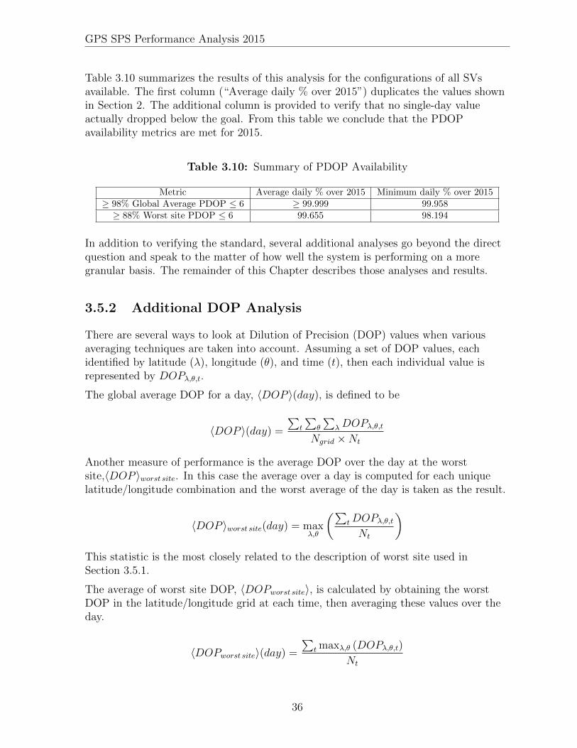
GPS SPS Performance Analysis 2015
Table 3.10 summarizes the results of this analysis for the configurations of all SVsavailable. The first column (“Average daily % over 2015”) duplicates the values shownin Section 2. The additional column is provided to verify that no single-day valueactually dropped below the goal. From this table we conclude that the PDOPavailability metrics are met for 2015.
Table 3.10: Summary of PDOP Availability
Metric Average daily % over 2015 Minimum daily % over 2015≥ 98% Global Average PDOP ≤ 6 ≥ 99.999 99.958≥ 88% Worst site PDOP ≤ 6 99.655 98.194
In addition to verifying the standard, several additional analyses go beyond the directquestion and speak to the matter of how well the system is performing on a moregranular basis. The remainder of this Chapter describes those analyses and results.
3.5.2 Additional DOP Analysis
There are several ways to look at Dilution of Precision (DOP) values when variousaveraging techniques are taken into account. Assuming a set of DOP values, eachidentified by latitude (λ), longitude (θ), and time (t), then each individual value isrepresented by DOPλ,θ,t.
The global average DOP for a day, 〈DOP 〉(day), is defined to be
〈DOP 〉(day) =
∑t
∑θ
∑λDOPλ,θ,t
Ngrid ×Nt
Another measure of performance is the average DOP over the day at the worstsite,〈DOP 〉worst site. In this case the average over a day is computed for each uniquelatitude/longitude combination and the worst average of the day is taken as the result.
〈DOP 〉worst site(day) = maxλ,θ
(∑tDOPλ,θ,tNt
)This statistic is the most closely related to the description of worst site used inSection 3.5.1.
The average of worst site DOP, 〈DOPworst site〉, is calculated by obtaining the worstDOP in the latitude/longitude grid at each time, then averaging these values over theday.
〈DOPworst site〉(day) =
∑t maxλ,θ (DOPλ,θ,t)
Nt
36

GPS SPS Performance Analysis 2015
This represents a measure of the worst DOP performance. It is not particularly usefulfrom the user’s point of view because the location of the worst site varies throughoutthe day.
Finally, the absolute worst time-point in a day is given by taking the maximum of theindividual DOP values for all locations and all times.
DOPabs. worst(day) = maxλ,θ,t
(DOPλ,θ,t)
Given that the 〈DOP 〉worst site(day) is most closely related to the worse site definitionused in Section 3.5.1, this is the statistic that will be used for “worst site” in theremainder of this section. For 2015, both 〈DOP 〉worst site(day) and 〈DOPworst site〉(day)satisfy the SPS PS assertions.
It is worth noting the following mathematical relationship between these quantities:
〈DOP 〉 ≤ 〈DOP 〉worst site ≤ 〈DOPworst site〉 ≤ DOPabs. worst
This serves as a sanity check on the DOP results in general and establishes that thesemetrics are increasingly sensitive to outliers.
In calculating the percentage of the time that the 〈DOP 〉 and 〈DOP 〉worst site arewithin bounds, several other statistics were calculated which provide insight into theavailability of the GPS constellation throughout the world. Included in these statisticsare the annual means of the daily globally average DOP and the 〈DOP 〉worst site values.These values are presented in Table 3.11, with values for 2012 through 2014 providedfor comparison. The average number of satellites and the fewest satellites visible acrossthe grid are calculated as part of the DOP calculations. Also shown in Table 3.11 arethe annual means of the global average number of satellites visible to grid cells on a 111km × 111 km (latitude by longitude) global grid and the annual means of the numberof satellites in the worst-site grid cell (defined as seeing the fewest number of satellites).It should be noted that the worst site for each of these values was not only determinedindependently from day-to-day, it was also determined independently for each metric.That is to say, it is not guaranteed that the worst site with respect to Horizontal DOP(HDOP) is the same as the worst site with respect to PDOP. For all quantities shownin Table 3.11 the values are very similar across all four years.
There are a few other statistics that can add insight regarding the GPS systemavailability. The primary availability metric requires that the globally averaged PDOPbe in-bounds at least 98% of the time. There are two related values: the number of daysfor which the PDOP is in bounds and the 98th percentile of the daily globally averagedPDOP values. Similarly, calculations can be done for 〈DOP 〉worst site criteria of havingthe PDOP ≤ 6 greater than 88% of the time. Table 3.12 presents these values.
Table 3.12 shows that the average DOP values for 2015 are nearly identical to previousyears.
37

GPS SPS Performance Analysis 2015
Table 3.11: Additional DOP Annually-Averaged Visibility Statistics for 2012 through2015
〈DOP 〉 〈DOP 〉worst site
2015 2014 2013 2012 2015 2014 2013 2012Horizontal DOP 0.85 0.86 0.83 0.84 0.97 0.99 0.96 0.96
Vertical DOP 1.37 1.39 1.35 1.36 1.71 1.73 1.69 1.69Time DOP 0.70 0.81 0.78 0.79 0.92 0.94 0.91 0.91
Position DOP 1.62 1.64 1.59 1.60 1.88 1.89 1.85 1.85Geometry DOP 1.81 1.83 1.77 1.79 2.08 2.10 2.05 2.05
Number of visible SVs 10.33 10.30 10.71 10.44 5.16 4.97 5.65 5.94
Table 3.12: Additional PDOP Statistics
2015 2014 2013 2012Percentage of Days with the 〈PDOP 〉 ≤ 6 100 100 100 100
Percentage of Days with the 〈PDOP 〉 at Worst Site ≤ 6 100 100 100 10098th Percentile of 〈PDOP 〉 1.65 1.67 1.63 1.65
88th Percentile of 〈PDOP 〉worst site 1.91 1.91 1.88 1.87
Behind the statistics are the day-to-day variations. Figure 3.12 provides a time historyof the four PDOP metrics considering all satellites for 2015. Four metrics are plotted:
• Daily Global Average PDOP, 〈PDOP 〉
• Average Worst Site PDOP, 〈PDOP 〉worst site
• Average PDOP at Worst Site, 〈PDOPworst site〉
• Absolute Worst PDOP, PDOPabs. worst
PDOPabs. worst is most sensitive to outliers and has features that are idiosyncratic to theparticular events in a year, such as SV outages. This is because PDOPabs. worst is theonly quantity that does not include averaging.
38

GPS SPS Performance Analysis 2015
Figure 3.12: Daily PDOP Metrics Using all SVs, 2015
The PDOPabs. worst trace for 2015 shown in Figure 3.12 has several features that wereexamined in further detail.
The large values on days 064, 071, 105, 132, 177, and 245 are each the result of singleSVs being set unhealthy. The SVs and NANUs are listed in Table 3.13. Generally,these spikes are of limited duration and effect only a small area at a given moment.
The elevated worst DOP time-history trace between Day 035 and Day 316 inFigure 3.12 is not typical. (Figures for the previous two years are provided inFigure 3.13 and Figure 3.14 for comparison.) Despite the appearance of highworst-point PDOP values, it is unlikely that this presented a problem to users. Thesehigh worst-point PDOP values were very short duration spikes (generally less than aminute) that were visible in very small areas.
As an example, we’ll describe the situation surrounding the worst point value on Day035. The daily analysis indicates a maximum value located at 63.00 N, 36.44 E at time01:11. Table 3.14 summarizes a DOP analysis for this location at one second intervals.The left side of Table 3.14 shows the situation on Day 034, when there was no largevalue observed. The right side of Table 3.14 shows the situation on Day 035, when thelarge values occurred. The two tables are aligned such that each row corresponds to the
39

GPS SPS Performance Analysis 2015
Figure 3.13: Daily PDOP Metrics Using All SVs, 2013
Figure 3.14: Daily PDOP Metrics Using All SVs, 2014
40
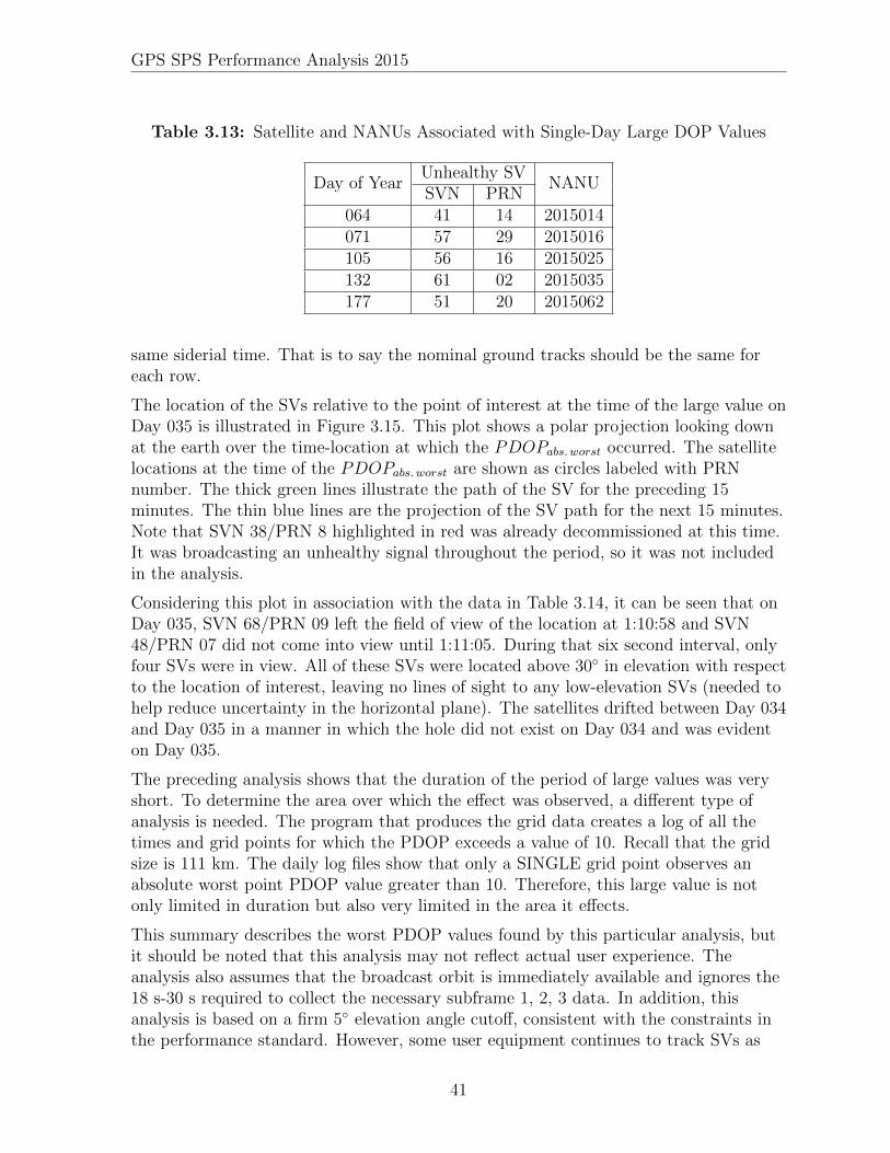
GPS SPS Performance Analysis 2015
Table 3.13: Satellite and NANUs Associated with Single-Day Large DOP Values
Unhealthy SVDay of Year
SVN PRNNANU
064 41 14 2015014071 57 29 2015016105 56 16 2015025132 61 02 2015035177 51 20 2015062
same siderial time. That is to say the nominal ground tracks should be the same foreach row.
The location of the SVs relative to the point of interest at the time of the large value onDay 035 is illustrated in Figure 3.15. This plot shows a polar projection looking downat the earth over the time-location at which the PDOPabs. worst occurred. The satellitelocations at the time of the PDOPabs. worst are shown as circles labeled with PRNnumber. The thick green lines illustrate the path of the SV for the preceding 15minutes. The thin blue lines are the projection of the SV path for the next 15 minutes.Note that SVN 38/PRN 8 highlighted in red was already decommissioned at this time.It was broadcasting an unhealthy signal throughout the period, so it was not includedin the analysis.
Considering this plot in association with the data in Table 3.14, it can be seen that onDay 035, SVN 68/PRN 09 left the field of view of the location at 1:10:58 and SVN48/PRN 07 did not come into view until 1:11:05. During that six second interval, onlyfour SVs were in view. All of these SVs were located above 30◦ in elevation with respectto the location of interest, leaving no lines of sight to any low-elevation SVs (needed tohelp reduce uncertainty in the horizontal plane). The satellites drifted between Day 034and Day 035 in a manner in which the hole did not exist on Day 034 and was evidenton Day 035.
The preceding analysis shows that the duration of the period of large values was veryshort. To determine the area over which the effect was observed, a different type ofanalysis is needed. The program that produces the grid data creates a log of all thetimes and grid points for which the PDOP exceeds a value of 10. Recall that the gridsize is 111 km. The daily log files show that only a SINGLE grid point observes anabsolute worst point PDOP value greater than 10. Therefore, this large value is notonly limited in duration but also very limited in the area it effects.
This summary describes the worst PDOP values found by this particular analysis, butit should be noted that this analysis may not reflect actual user experience. Theanalysis also assumes that the broadcast orbit is immediately available and ignores the18 s-30 s required to collect the necessary subframe 1, 2, 3 data. In addition, thisanalysis is based on a firm 5◦ elevation angle cutoff, consistent with the constraints inthe performance standard. However, some user equipment continues to track SVs as
41

GPS SPS Performance Analysis 2015
Table 3.14: DOP Results for 63N, 36.44E on Day 34/35
Day 034 Day 035HH:MM:SS PDOP #SVs List of SVs HH:MM:SS PDOP #SVs List of SVs
01:14:35 1.8 6 5 9 16 21 25 29 01:10:39 1.8 6 5 9 16 21 25 2901:14:36 1.8 6 01:10:40 1.8 601:14:37 1.8 6 01:10:41 1.8 601:14:38 1.8 6 01:10:42 4.6 5 5 9 16 21 2901:14:39 1.8 6 01:10:43 4.6 501:14:40 1.8 6 01:10:44 4.6 501:14:41 1.8 6 01:10:45 4.6 501:14:42 1.8 6 01:10:46 4.6 501:14:43 1.8 6 01:10:47 4.6 501:14:44 1.8 6 01:10:48 4.6 501:14:45 4.6 5 5 9 16 21 29 01:10:49 4.6 501:14:46 4.6 5 01:10:50 4.6 501:14:47 4.6 5 01:10:51 4.6 501:14:48 4.6 5 01:10:52 4.6 501:14:49 4.6 5 01:10:53 4.6 501:14:50 4.6 5 01:10:54 4.6 501:14:51 4.6 5 01:10:55 4.6 501:14:52 4.6 5 01:10:56 4.6 501:14:53 4.6 5 01:10:57 4.6 501:14:54 4.6 5 01:10:58 4.6 501:14:55 4.6 5 01:10:59 1997.9 4 5 16 21 2901:14:56 4.6 5 01:11:00 1719.7 401:14:57 4.6 5 01:11:01 1509.5 401:14:58 4.6 5 01:11:02 1345.1 401:14:59 4.6 5 01:11:03 1213.0 401:15:00 4.6 5 01:11:04 1104.5 401:15:01 4.6 5 01:11:05 4.8 5 5 7 16 21 2901:15:02 4.6 5 01:11:06 4.8 501:15:03 4.6 5 01:11:07 4.8 501:15:04 4.6 5 01:11:08 4.8 501:15:05 4.6 5 01:11:09 4.8 501:15:06 4.8 5 5 7 16 21 29a 01:11:10 4.8 501:15:07 4.8 5 01:11:11 4.8 501:15:08 4.8 5 01:11:12 4.8 501:15:09 4.8 5 01:11:13 4.8 5
b- - - - - -01:15:21 4.8 5 01:11:25 4.8 501:15:22 4.8 5 01:11:26 4.8 501:15:23 4.8 5 01:11:27 4.8 501:15:24 4.8 5 01:11:28 4.8 501:15:25 4.8 5 01:11:29 1.8 6 5 7 16 18 21 2901:15:26 4.8 5 01:11:30 1.8 601:15:27 4.8 5 01:11:31 1.8 601:15:28 4.8 5 01:11:32 1.8 601:15:29 4.8 5 01:11:33 1.8 601:15:30 4.8 5 01:11:34 1.8 601:15:31 1.8 6 5 7 16 18 21 29 01:11:35 1.8 601:15:32 1.8 6 01:11:36 1.8 601:15:33 1.8 6 01:11:37 1.8 601:15:34 1.8 6 01:11:38 1.8 6
aNote that one SV was dropped (PRN 9) and one added (PRN 7) within a one-second interval.b12 seconds of repeated data omitted.
42

GPS SPS Performance Analysis 2015
Figure 3.15: GPS Visibility on Day 035 at 01:11 Relative to 63N, 36.44E
43
GPS SPS Performance Analysis 2015
low as possible until the signal is lost. Such a receiver may not have experienced theselarge values as other SVs came into view providing alternate means of achieving goodPDOP values prior to losing the SV dropping below 5◦. In addition, given the veryshort durations of these worst points, implementations that differed on how to roundthe elevation angle value could achieve different results.
As a result, we conclude that in 2015 there existed a larger-than-normal probabilitythat high PDOP values might be observed over small areas for very short periods oftime. However, the user impact was almost certainly negligible. In addition, these shortevents do not result in a violation of any of the assertions in the performance standards.
3.5.3 Position Service Availability
The positioning and timing availability standards are stated in Table 3.8-2 of SPSPS08as follows:
• “≥ 99% Horizontal Service Availability, average location”
• “≥ 99% Vertical Service Availability, average location”
• “≥ 90% Horizontal Service Availability, worst-case location”
• “≥ 90% Vertical Service Availability, worst-case location”
The conditions and constraints associated with the standards include the specificationof a 17 m horizontal 95th percentile threshold and a 37 m vertical 95th percentilethreshold.
These are derived values as described in the sentence preceding SPSPS08 Table 3.8-2:
“The commitments for maintaining PDOP (Table 3.8-1) and SPS SIS UREaccuracy (Table 3.4-1) result in support for position service availabilitystandards as presented in Table 3.8-2.”
Because the commitments for PDOP and constellation SPS SIS URE have not onlybeen met, but exceeded, this assertion in the SPSPS08 implies that the position andtiming availability standards have also been fulfilled. A direct assessment of thesemetrics was not undertaken.
3.5.4 Position Accuracy
The positioning accuracy standards are stated in Table 3.8-3 of SPSPS08 as follows:
• “≤ 9 m 95% Horizontal Error Global Average Position Domain Accuracy”
44

GPS SPS Performance Analysis 2015
• “≤ 15 m 95% Vertical Error Global Average Position Domain Accuracy”
• “≤ 17 m 95% Horizontal Error Worst Site Position Domain Accuracy”
• “≤ 37 m 95% Vertical Error Worst Site Position Domain Accuracy”
These are derived values as described in the sentence preceding SPSPS08 Table 3.8-3:
“The commitments for maintaining PDOP (Table 3.8-1) and SPS SIS UREaccuracy (Table 3.4-1) result in support for position service availabilitystandards as presented in Table 3.8-3.”
Because the commitments for PDOP and constellation SPS SIS URE have been metand exceeded, then the position and timing accuracy standards have also been fulfilled.
While this answer is technically correct, it is not very helpful. Position accuracy is theprimary reason that GPS exists. At the same time, position accuracy is a particularlydifficult metric to evaluate due to the fact that GPS provides the SIS, but the user isresponsible for appropriately processing the SIS to derive a position.
Section 2.4.5 of SPSPS08 provides usage assumptions for the SPS PS and some of thenotes in Section 2.4.5 are relevant to the question of position determination. Thefollowing is quoted from section 2.4.5:
“The performance standards in Section 3 of this SPS PS do not take intoconsideration any error source that is not under direct control of the SpaceSegment or Control Segment. Specifically excluded errors include those dueto the effects of:
• Signal distortions caused by ionospheric and/or troposphericscintillation
• Residual receiver ionospheric delay compensation errors
• Residual receiver tropospheric delay compensation errors
• Receiver noise (including received signal power and interference power)and resolution
• Multipath and receiver multipath mitigation
• User antenna effects
• Operator (user) error”
In addition, at the beginning of Section 3.8, the SPSPS08 explains that in addition tothe error exclusions listed in 2.4.5, the following assumptions are made regarding theSPS receiver:
“The use of a representative SPS receiver that:
45

GPS SPS Performance Analysis 2015
• is designed in accordance with IS-GPS-200
• is tracking the SPS SIS from all satellites in view above a 5◦ maskangle... It is assumed the receiver is operating in a nominal noiseenvironment...
• accomplishes satellite position and geometric range computations in themost current realization of the WGS 84 Earth-Centered, Earth-Fixed(ECEF) coordinate system.
• generates a position and time solution from data broadcast by allsatellites in view
• compensates for dynamic Doppler shift effects on nominal SPS rangingsignal carrier phase and C/A code measurements.
• processes the health-related information in the SIS and excludesmarginal and unhealthy SIS from the position solution.
• ensures the use of up-to-date and internally consistent ephemeris andclock data for all satellites it is using in its position solution.
• loses track in the event a GPS satellite stops transmitting a trackableSIS.
• is operating at a surveyed location (for a time transfer receiver).”
ARL:UT adopted the following approach for computing a set of accuracy statistics:
1. 30 s GPS observations were collected from the NGA GPS monitor stationnetwork and a similar set of 18 IGS stations. This decision addressed thefollowing concerns:
(a) All stations selected collect dual-frequency observations. Therefore thefirst-order ionospheric effects can be eliminated from the results.
(b) All stations selected collect weather observations. The program thatgenerates the positions (PRSOLVE) uses the weather data to eliminate firstorder tropospheric effects.
(c) The receiver thermal noise will not be eliminated, but both the NGA andIGS stations are generally using the best available equipment, so effects willbe limited.
(d) Similarly, multipath cannot be eliminated, but both networks use antennasdesigned for multipath reduction, and station sites are chosen to avoid theintroduction of extraneous multipath.
(e) Antenna phase center locations for such stations are very well known.Therefore, position truth is readily available.
2. Process the data using a comprehensive set of broadcast ephemerides that havebeen checked for consistency. The set of ephemerides used in the URE studies
46

GPS SPS Performance Analysis 2015
described in Section 3.1 of this report had already been extensively tested andexamined. They constitute a complete (or very nearly complete) set of thebroadcast ephemeris available for 2015.
3. Process the collected observations using the PRSOLVE program of theARL:UT-hosted open source GPS Toolkit (GPSTk)[9]. Note:
(a) PRSOLVE meets the relevant requirements listed above. For example, SVpositions are derived in accordance with IS-GPS-200, the elevation mask isconfigurable, weather data is used to estimate tropospheric effects, and WGS84 [10] conventions are used. Data from unhealthy SVs were removed fromPRSOLVE using an option to exclude specific satellites.
(b) PRSOLVE is highly configurable. Several of the items in the preceding list ofassumptions are configuration parameters to PRSOLVE.
(c) Any other organization that wishes to reproduce the results should be ableto do so. (Both the algorithm and the IGS data are available.)
4. Process the collected 30 s observations in two ways:
(a) Use all SVs in view without data editing in an autonomous pseudorangesolution to generate 30 s position residuals at all sites.
(b) Use a receiver autonomous integrity monitoring (RAIM) algorithm (anotherPRSOLVE option) to remove outlier pseudorange measurements from whicha “clean” set of 30 s position residuals is generated at all sites. The RAIMalgorithm used by PRSOLVE is dependent on several parameters, the twomost important of which are the RMS limit on the post-fit residuals (default:3.0 m) and the number of SVs that can be eliminated in the RAIM process(default: unlimited). This analysis was conducted using the default values.
5. Compute statistics on each set of data independently.
In contrast to previous years, we conducted the elevation angle processing with a 5◦
minimum elevation angle for greater agreement with the standard. (Previous years wereprocessed with a 10◦ minimum elevation angle.)
This process yields four sets of results organized as detailed in Table 3.15.
Table 3.15: Organization of Positioning Results
Case Constellation Considered Data Editing Option Data Source1
All in ViewRAIM
IGS Data2 NGA Data3
NoneIGS Data
4 NGA Data
47
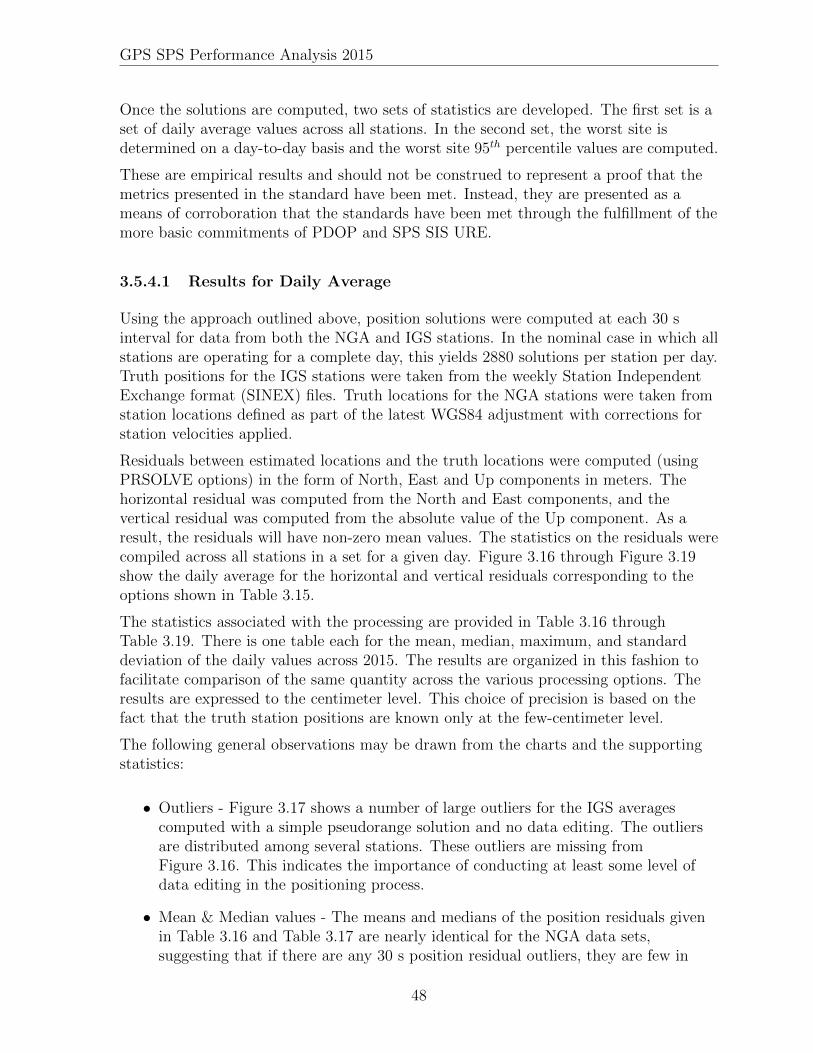
GPS SPS Performance Analysis 2015
Once the solutions are computed, two sets of statistics are developed. The first set is aset of daily average values across all stations. In the second set, the worst site isdetermined on a day-to-day basis and the worst site 95th percentile values are computed.
These are empirical results and should not be construed to represent a proof that themetrics presented in the standard have been met. Instead, they are presented as ameans of corroboration that the standards have been met through the fulfillment of themore basic commitments of PDOP and SPS SIS URE.
3.5.4.1 Results for Daily Average
Using the approach outlined above, position solutions were computed at each 30 sinterval for data from both the NGA and IGS stations. In the nominal case in which allstations are operating for a complete day, this yields 2880 solutions per station per day.Truth positions for the IGS stations were taken from the weekly Station IndependentExchange format (SINEX) files. Truth locations for the NGA stations were taken fromstation locations defined as part of the latest WGS84 adjustment with corrections forstation velocities applied.
Residuals between estimated locations and the truth locations were computed (usingPRSOLVE options) in the form of North, East and Up components in meters. Thehorizontal residual was computed from the North and East components, and thevertical residual was computed from the absolute value of the Up component. As aresult, the residuals will have non-zero mean values. The statistics on the residuals werecompiled across all stations in a set for a given day. Figure 3.16 through Figure 3.19show the daily average for the horizontal and vertical residuals corresponding to theoptions shown in Table 3.15.
The statistics associated with the processing are provided in Table 3.16 throughTable 3.19. There is one table each for the mean, median, maximum, and standarddeviation of the daily values across 2015. The results are organized in this fashion tofacilitate comparison of the same quantity across the various processing options. Theresults are expressed to the centimeter level. This choice of precision is based on thefact that the truth station positions are known only at the few-centimeter level.
The following general observations may be drawn from the charts and the supportingstatistics:
• Outliers - Figure 3.17 shows a number of large outliers for the IGS averagescomputed with a simple pseudorange solution and no data editing. The outliersare distributed among several stations. These outliers are missing fromFigure 3.16. This indicates the importance of conducting at least some level ofdata editing in the positioning process.
• Mean & Median values - The means and medians of the position residuals givenin Table 3.16 and Table 3.17 are nearly identical for the NGA data sets,suggesting that if there are any 30 s position residual outliers, they are few in
48

GPS SPS Performance Analysis 2015
Table 3.16: Mean of Daily Average Position Errors for 2015
Quantity Data SourcePosition Residual Mean (m)
RAIM No Editing
HorizontalIGS Data 1.37 8.09
NGA Data 1.08 1.10
VerticalIGS Data 2.10 10.56
NGA Data 1.46 1.49
Table 3.17: Median of Daily Average Position Errors for 2015
Quantity Data SourcePosition Residual Median (m)
RAIM No Editing
HorizontalIGS Data 1.38 1.42
NGA Data 1.08 1.09
VerticalIGS Data 2.10 2.18
NGA Data 1.45 1.48
Table 3.18: Maximum of Daily Average Position Errors for 2015
Quantity Data SourcePosition Residual Maximum (m)
RAIM No Editing
HorizontalIGS Data 1.57 262.05
NGA Data 1.17 1.25
VerticalIGS Data 2.44 176.48
NGA Data 1.61 1.77
Table 3.19: Standard Deviation of Daily Average Position Errors for 2015
Quantity Data SourcePosition Residual Std. Dev. (m)
RAIM No Editing
HorizontalIGS Data 0.05 22.22
NGA Data 0.03 0.04
VerticalIGS Data 0.09 22.91
NGA Data 0.04 0.06
49

GPS SPS Performance Analysis 2015
Jan Feb
Mar Apr May Jun Jul Aug Sep
Oct Nov Dec
Month, 2015
0
5
10
15
20
Aver
age
Erro
r (m
)SPS PS Vert Limit
SPS PS Horiz Limit
Averages of Position ErrorAll SVs, RAIM Solution
Avg Vert NGA Avg Horiz NGA Avg Vert IGS Avg Horiz IGS
Figure 3.16: Daily Averaged Position Residuals Computed Using a RAIM Solution
Jan Feb
Mar Apr May Jun Jul Aug Sep
Oct Nov Dec
Month, 2015
101
102
103
104
Aver
age
Erro
r (m
)
SPS PS Vert Limit
SPS PS Horiz Limit
Averages of Position ErrorAll SVs, Pseudorange Solution
Avg Vert NGA Avg Horiz NGA Avg Vert IGS Avg Horiz IGS
Figure 3.17: Daily Averaged Position Residuals Computed Using No Data Editing
50
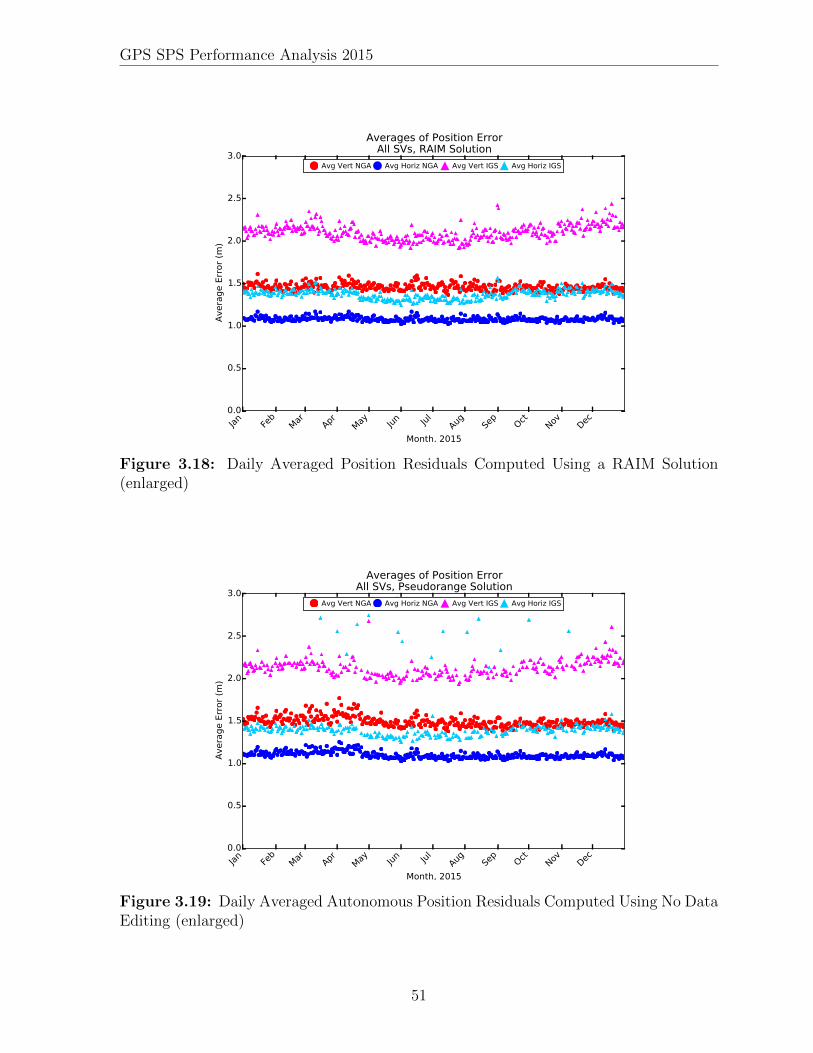
GPS SPS Performance Analysis 2015
Jan Feb
Mar Apr May Jun Jul Aug Sep
Oct Nov Dec
Month, 2015
0.0
0.5
1.0
1.5
2.0
2.5
3.0
Aver
age
Erro
r (m
)
Averages of Position ErrorAll SVs, RAIM Solution
Avg Vert NGA Avg Horiz NGA Avg Vert IGS Avg Horiz IGS
Figure 3.18: Daily Averaged Position Residuals Computed Using a RAIM Solution(enlarged)
Jan Feb
Mar Apr May Jun Jul Aug Sep
Oct Nov Dec
Month, 2015
0.0
0.5
1.0
1.5
2.0
2.5
3.0
Aver
age
Erro
r (m
)
Averages of Position ErrorAll SVs, Pseudorange Solution
Avg Vert NGA Avg Horiz NGA Avg Vert IGS Avg Horiz IGS
Figure 3.19: Daily Averaged Autonomous Position Residuals Computed Using No DataEditing (enlarged)
51

GPS SPS Performance Analysis 2015
number and not too large. This also holds true for the RAIM solutions from theIGS data sets. However, the means and medians for the IGS data set solutionswith no data editing are very different. This is consistent with the outliersobserved in Figure 3.17 and with the maximum and standard deviation values forthe IGS data set solutions. This suggest that there are some large 30 s positionresiduals in the epoch-by-epoch results for these data sets.
• Differences between NGA and IGS results - The average magnitude of theposition residual as reported in Table 3.16 is slightly smaller for the NGA stationsthan for the IGS stations. There are a number of differences between the twostation sets. The NGA station set is more homogeneous in that the same receivermodel is used throughout the data processed for this analysis, the data arederived from full-code tracking, and a single organization prepared all the datasets using a single set of algorithms. By contrast, the IGS data sets come from avariety of receivers and were prepared and submitted by a variety oforganizations. These differences likely account for the greater variability in theresults derived from the IGS data sets.
3.5.4.2 Results for Worst Site 95th Percentile
The edited, and the non-edited, 30 s position residuals were then processed(independently) to determine the worst site 95th percentile values. In this case, the 95th
percentile was determined for each station in a given set, and the worst of these wasused as the final 95th percentile value for that day. Figure 3.20 and Figure 3.21 showthese values for the various processing options described in the previous section. Theplots are followed by tables of the statistics for the average, median, maximum, andstandard deviation of the daily worst site 95th percentile values. Some generalobservations on the results are included following the tables.
The statistics associated with the worst site 95th percentile values are provided inTable 3.20 through Table 3.23. There is one table each for the average, median,maximum, and standard deviation of the daily values across 2015. As before, theresults are organized in this fashion to facilitate comparison of the same quantity acrossthe various processing options. Precisions are chosen to be at the centimeter level, achoice based on:
• The magnitude of the standard deviation.
• The fact that the station positions are known only at the few-centimeter level.
Most of the observations from the daily averages hold true in the case of the results forthe worst site 95th percentile case. However, there are a few additional observations:
• Comparison to threshold - The values for both mean and median of the worst95th percentile for both horizontal and vertical errors are well within the standard
52

GPS SPS Performance Analysis 2015
for both solutions. Compared to the thresholds of 17 m 95th percentile horizontaland 37 m 95th percentile vertical these results are outstanding.
• Comparison between processing options - The statistics for the RAIM solutionsare slightly better than the statistics for the pseudorange solutions with respect tomean and median. However, the worst values (Table 3.22) for the IGS data withno editing exceed the 95th percentile error worst site assertion. This illustrates theimportance of some form of data editing.
53

GPS SPS Performance Analysis 2015
Jan Feb
Mar Apr May Jun Jul Aug Sep
Oct Nov Dec
Month, 2015
0
10
20
30
40
50
60
Wor
st 9
5th
Perc
entil
e Er
ror (
m)
Worst 95th Percentile of Daily Position ErrorsAll SVs, RAIM Solution
Vert NGA Horiz NGA Vert IGS Horiz IGS
SPS PS Vert Limit
SPS PS Horiz Limit
Figure 3.20: Worst Site 95th Daily Averaged Position Residuals Computed Using aRAIM Solution
Jan Feb
Mar Apr May Jun Jul Aug Sep
Oct Nov Dec
Month, 2015
0
10
20
30
40
50
60
Wor
st 9
5th
Perc
entil
e Er
ror (
m)
Worst 95th Percentile of Daily Position ErrorsAll SVs, Pseudorange Solution
Vert NGA Horiz NGA Vert IGS Horiz IGS
SPS PS Vert Limit
SPS PS Horiz Limit
Figure 3.21: Worst Site 95th Daily Averaged Position Residuals Computed Using NoData Editing
54
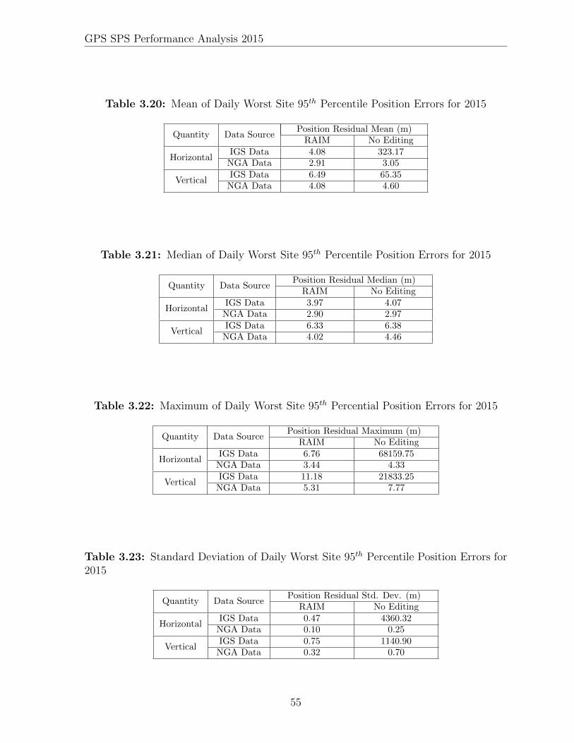
GPS SPS Performance Analysis 2015
Table 3.20: Mean of Daily Worst Site 95th Percentile Position Errors for 2015
Quantity Data SourcePosition Residual Mean (m)
RAIM No Editing
HorizontalIGS Data 4.08 323.17
NGA Data 2.91 3.05
VerticalIGS Data 6.49 65.35
NGA Data 4.08 4.60
Table 3.21: Median of Daily Worst Site 95th Percentile Position Errors for 2015
Quantity Data SourcePosition Residual Median (m)
RAIM No Editing
HorizontalIGS Data 3.97 4.07
NGA Data 2.90 2.97
VerticalIGS Data 6.33 6.38
NGA Data 4.02 4.46
Table 3.22: Maximum of Daily Worst Site 95th Percential Position Errors for 2015
Quantity Data SourcePosition Residual Maximum (m)
RAIM No Editing
HorizontalIGS Data 6.76 68159.75
NGA Data 3.44 4.33
VerticalIGS Data 11.18 21833.25
NGA Data 5.31 7.77
Table 3.23: Standard Deviation of Daily Worst Site 95th Percentile Position Errors for2015
Quantity Data SourcePosition Residual Std. Dev. (m)
RAIM No Editing
HorizontalIGS Data 0.47 4360.32
NGA Data 0.10 0.25
VerticalIGS Data 0.75 1140.90
NGA Data 0.32 0.70
55

Chapter 4
Additional Results of Interest
4.1 Frequency of Different SV Health States
Several of the assertions require examination of the health information transmitted byeach SV. We have found it useful to examine the rate of occurrence for all possiblecombinations of the six health bits transmitted in subframe 1.
Table 4.1 presents a summary of health bit usage in the ephemerides broadcast during2015. Each row in the table presents a summary for a specific SV. The summary acrossall SVs are shown at the bottom. The table contains the count of number of times eachunique health code was seen, the raw count of unique sets of subframe 1, 2, 3 collectedduring the year, and the percentage of sets of subframe 1, 2, 3 data that containedspecific health codes.
Only two unique health settings were observed throughout 2015: binary 0000002 (0x00)and binary 1111112 (0x3F).
4.2 Age of Data
The Age of Data (AOD) represents the elapsed time between the observations thatwere used to create the broadcast navigation message and the time when the contentsof subframes 1, 2, 3 are available to the user to estimate the position of a SV. Theaccuracy of GPS (at least for users that depend on the broadcast ephemeris) isindirectly tied to the AOD because the prediction accuracy degrades over time (seeSection 3.1.2). This is especially true for the clock prediction. It has been recognizedthat reducing the AOD improves position, velocity, or time (PVT) solutions forautonomous users; however, there is an impact in terms of increased operations tempoat 2nd Space Operations Squadron (2 SOPS).
Note that there is no need for a GPS receiver to refer to AOD in any PVT computationother than the optional application of the navigation message correction table (NMCT).
56
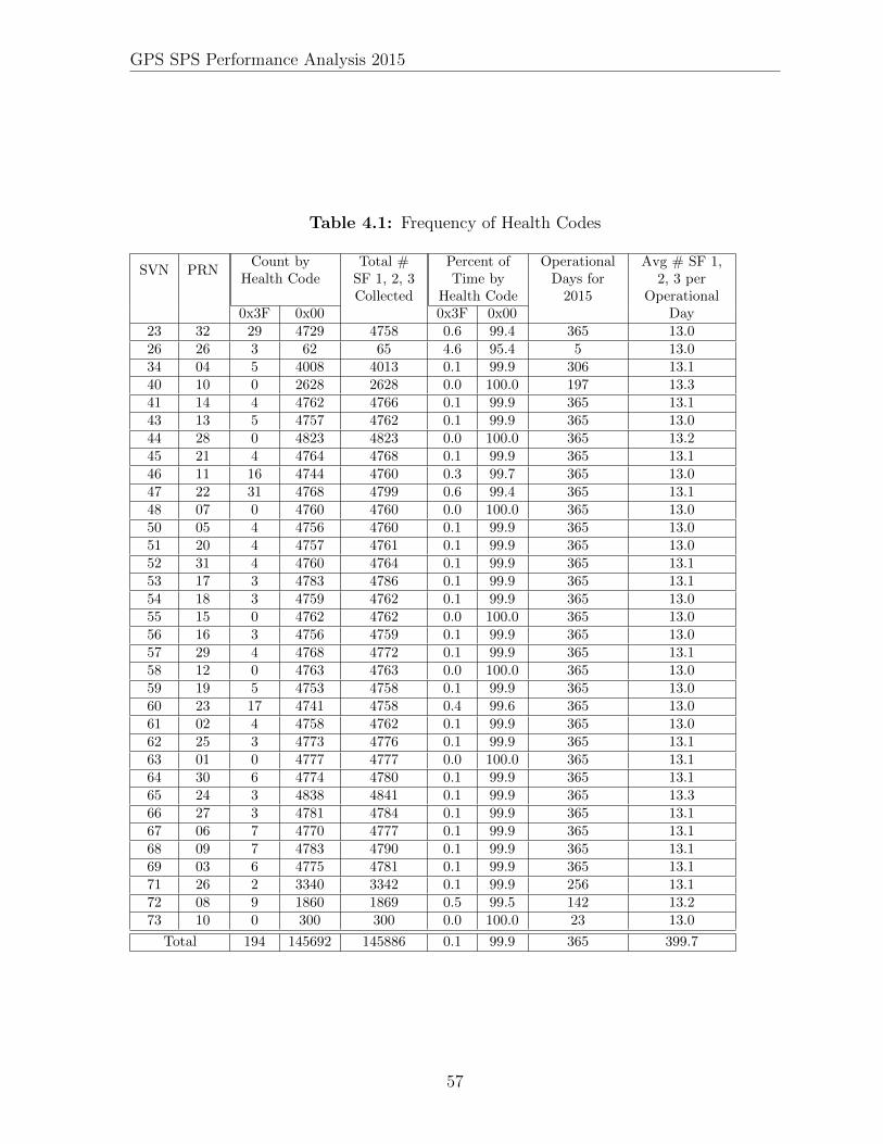
GPS SPS Performance Analysis 2015
Table 4.1: Frequency of Health Codes
SVN PRNCount by
Health CodeTotal #
SF 1, 2, 3Collected
Percent ofTime by
Health Code
OperationalDays for
2015
Avg # SF 1,2, 3 per
OperationalDay0x3F 0x00 0x3F 0x00
23 32 29 4729 4758 0.6 99.4 365 13.026 26 3 62 65 4.6 95.4 5 13.034 04 5 4008 4013 0.1 99.9 306 13.140 10 0 2628 2628 0.0 100.0 197 13.341 14 4 4762 4766 0.1 99.9 365 13.143 13 5 4757 4762 0.1 99.9 365 13.044 28 0 4823 4823 0.0 100.0 365 13.245 21 4 4764 4768 0.1 99.9 365 13.146 11 16 4744 4760 0.3 99.7 365 13.047 22 31 4768 4799 0.6 99.4 365 13.148 07 0 4760 4760 0.0 100.0 365 13.050 05 4 4756 4760 0.1 99.9 365 13.051 20 4 4757 4761 0.1 99.9 365 13.052 31 4 4760 4764 0.1 99.9 365 13.153 17 3 4783 4786 0.1 99.9 365 13.154 18 3 4759 4762 0.1 99.9 365 13.055 15 0 4762 4762 0.0 100.0 365 13.056 16 3 4756 4759 0.1 99.9 365 13.057 29 4 4768 4772 0.1 99.9 365 13.158 12 0 4763 4763 0.0 100.0 365 13.059 19 5 4753 4758 0.1 99.9 365 13.060 23 17 4741 4758 0.4 99.6 365 13.061 02 4 4758 4762 0.1 99.9 365 13.062 25 3 4773 4776 0.1 99.9 365 13.163 01 0 4777 4777 0.0 100.0 365 13.164 30 6 4774 4780 0.1 99.9 365 13.165 24 3 4838 4841 0.1 99.9 365 13.366 27 3 4781 4784 0.1 99.9 365 13.167 06 7 4770 4777 0.1 99.9 365 13.168 09 7 4783 4790 0.1 99.9 365 13.169 03 6 4775 4781 0.1 99.9 365 13.171 26 2 3340 3342 0.1 99.9 256 13.172 08 9 1860 1869 0.5 99.5 142 13.273 10 0 300 300 0.0 100.0 23 13.0
Total 194 145692 145886 0.1 99.9 365 399.7
57
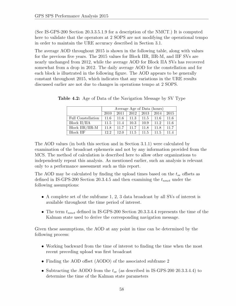
GPS SPS Performance Analysis 2015
(See IS-GPS-200 Section 20.3.3.5.1.9 for a description of the NMCT.) It is computedhere to validate that the operators at 2 SOPS are not modifying the operational tempoin order to maintain the URE accuracy described in Section 3.1.
The average AOD throughout 2015 is shown in the following table, along with valuesfor the previous five years. The 2015 values for Block IIR, IIR-M, and IIF SVs arenearly unchanged from 2012, while the average AOD for Block IIA SVs has recoveredsomewhat from a drop in 2012. The daily average AOD for the constellation and foreach block is illustrated in the following figure. The AOD appears to be generallyconstant throughout 2015, which indicates that any variations in the URE resultsdiscussed earlier are not due to changes in operations tempo at 2 SOPS.
Table 4.2: Age of Data of the Navigation Message by SV Type
Average Age of Data (hours)2010 2011 2012 2013 2014 2015
Full Constellation 11.6 11.6 11.3 11.5 11.6 11.6Block II/IIA 11.5 11.4 10.3 10.9 11.2 11.6Block IIR/IIR-M 11.8 11.7 11.7 11.8 11.8 11.7Block IIF 12.2 12.0 11.5 11.5 11.5 11.4
The AOD values (in both this section and in Section 3.1.1) were calculated byexamination of the broadcast ephemeris and not by any information provided from theMCS. The method of calculation is described here to allow other organizations toindependently repeat this analysis. As mentioned earlier, such an analysis is relevantonly to a performance assessment such as this report.
The AOD may be calculated by finding the upload times based on the toe offsets asdefined in IS-GPS-200 Section 20.3.4.5 and then examining the tnmct under thefollowing assumptions:
• A complete set of the subframe 1, 2, 3 data broadcast by all SVs of interest isavailable throughout the time period of interest.
• The term tnmct defined in IS-GPS-200 Section 20.3.3.4.4 represents the time of theKalman state used to derive the corresponding navigation message.
Given these assumptions, the AOD at any point in time can be determined by thefollowing process:
• Working backward from the time of interest to finding the time when the mostrecent preceding upload was first broadcast
• Finding the AOD offset (AODO) of the associated subframe 2
• Subtracting the AODO from the toe (as described in IS-GPS-200 20.3.3.4.4) todetermine the time of the Kalman state parameters
58

GPS SPS Performance Analysis 2015
Figure 4.1: Constellation Age of Data for 2015
• Calculating the difference between the time of interest and the Kalman stateparameter time
The search for the preceding upload is necessary because the AODO has a limited rangeand is not sufficiently large to maintain an accurate count for a complete upload cycle.
The results of this algorithm are generally consistent with the results provided by MCSanalysis. The first assumption is fulfilled by the NGA MSN archive. The remainingassumptions were discussed with systems engineers supporting 2 SOPS and are believedto be valid.
4.3 User Range Accuracy Index Trends
Tables 4.3 on page 61 and 4.4 on page 62 present a summary of the analysis of theURA index values throughout 2015. The total number of navigation messagesexamined differs from the health summary in Section 4.1 because only URA indexvalues corresponding to health settings of 0x00 are included in this analysis. Both theabsolute count and the count as a percentage of the total are shown.
59
GPS SPS Performance Analysis 2015
The vast majority of the values are 0, 1, or 2 (over 99.9%). Index values between 3 and5 were very rare. No values over 5 were observed.
4.4 Extended Mode Operations
IS-GPS-200 defines Normal Operations as the period of time when subframe 1, 2, 3data sets are transmitted by the SV for periods of two hours with a curve fit interval offour hours (IS-GPS-200 Section 20.3.4.4). This definition is taken to be the same as thedefinition of Normal Operations in SPSPS08 for the URE metrics. To determine if anySV operated in other than Normal Operations at any time in 2015, the broadcastephemerides were examined to determine if any contained fit interval flags set to 1. (SeeIS-GPS-200 20.3.3.4.3.1 for definition of the fit interval flag.)
The analysis found a total of 48 examples of extended operations for satellites sethealthy. The examples were distributed across 34 days. The average time of anoccurrence was 50 minutes. The minimum duration was 150 seconds and the maximumduration was 5 hours 35 minutes. These results are summarized in Table 4.5 on page 63.
Given the relative rarity of occurrence, the URE values for the periods summarized inTable 4.5 are included in the statistics presented in Section 3.1.1, even though a strictinterpretation of the SPSPS08 would suggest that they be removed. However, the SVsinvolved were still set healthy and (presumably) being used by user equipment, it isappropriate to include these results to reflect performance seen by the users.
Examination of the ephemerides from past years reveals that 2015 is not an anomaly.Such periods have been found in all years checked (back to 2005).
Past discussions with the operators have revealed several reasons for these occurrences.Some are associated with Alternate MCS (AMCS) testing. When operations aretransitioned from the MCS to the AMCS (and reverse) it is possible that SVs nearingthe end of their daily cycle may experience a longer-than-normal upload cycle. Otheroccurrences may be caused by delays due to ground antenna maintenance or due tooperator concentration on higher-priority issues with the constellation at the time.
60

GPS SPS Performance Analysis 2015
Table 4.3: Distribution of URA Index Values
SVN PRNURA Index Total #
SF 1, 2,3
examined
Oper.Daysfor
2015
Avg #SF 1, 2,
3 perOper.Day
5 4 3 2 1 023 32 236 4493 4729 365 13.026 26 10 52 62 5 12.434 04 1 180 3827 4008 306 13.140 10 85 797 1746 2628 197 13.341 14 25 829 3908 4762 365 13.043 13 3 331 4423 4757 365 13.044 28 3 910 3910 4823 365 13.245 21 11 485 1011 3257 4764 365 13.146 11 4 417 4323 4744 365 13.047 22 1 217 1291 3259 4768 364 13.148 07 23 224 397 4116 4760 365 13.050 05 2 5 179 4570 4756 365 13.051 20 2 100 4655 4757 365 13.052 31 2 1 5 226 4526 4760 365 13.053 17 2 5 1 8 584 4183 4783 365 13.154 18 1 6 185 4567 4759 365 13.055 15 1 301 4460 4762 365 13.056 16 3 293 4460 4756 365 13.057 29 584 4184 4768 365 13.158 12 228 4535 4763 365 13.059 19 267 4486 4753 365 13.060 23 2 286 4453 4741 365 13.061 02 4 51 4703 4758 365 13.062 25 1 232 4540 4773 365 13.163 01 62 4715 4777 365 13.164 30 1 8 239 4526 4774 365 13.165 24 3 1020 3815 4838 365 13.366 27 176 4605 4781 365 13.167 06 2 83 4685 4770 365 13.168 09 0 311 4472 4783 365 13.169 03 1 5 2 7 632 4128 4775 365 13.171 26 368 2972 3340 256 13.072 08 80 426 1354 1860 142 13.173 10 2 44 254 300 23 13.0
Total 3 12 43 1186 13286 131162 145692 365 399.2
61
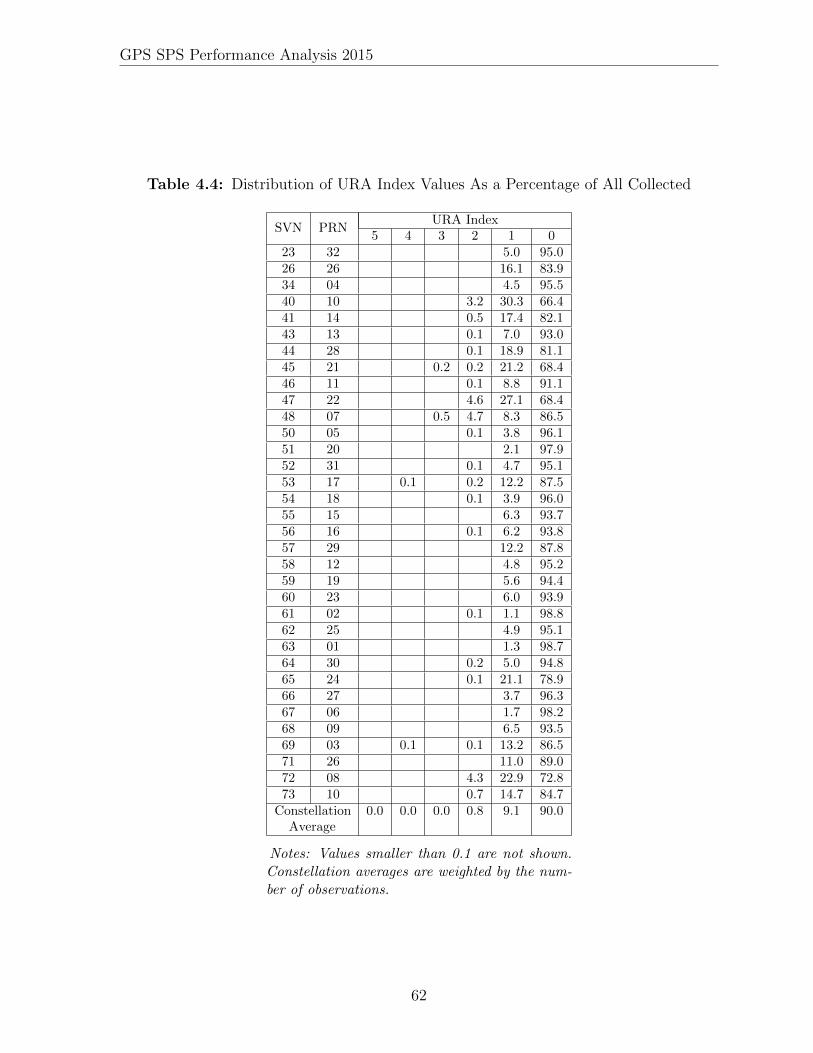
GPS SPS Performance Analysis 2015
Table 4.4: Distribution of URA Index Values As a Percentage of All Collected
SVN PRNURA Index
5 4 3 2 1 023 32 5.0 95.026 26 16.1 83.934 04 4.5 95.540 10 3.2 30.3 66.441 14 0.5 17.4 82.143 13 0.1 7.0 93.044 28 0.1 18.9 81.145 21 0.2 0.2 21.2 68.446 11 0.1 8.8 91.147 22 4.6 27.1 68.448 07 0.5 4.7 8.3 86.550 05 0.1 3.8 96.151 20 2.1 97.952 31 0.1 4.7 95.153 17 0.1 0.2 12.2 87.554 18 0.1 3.9 96.055 15 6.3 93.756 16 0.1 6.2 93.857 29 12.2 87.858 12 4.8 95.259 19 5.6 94.460 23 6.0 93.961 02 0.1 1.1 98.862 25 4.9 95.163 01 1.3 98.764 30 0.2 5.0 94.865 24 0.1 21.1 78.966 27 3.7 96.367 06 1.7 98.268 09 6.5 93.569 03 0.1 0.1 13.2 86.571 26 11.0 89.072 08 4.3 22.9 72.873 10 0.7 14.7 84.7
ConstellationAverage
0.0 0.0 0.0 0.8 9.1 90.0
Notes: Values smaller than 0.1 are not shown.Constellation averages are weighted by the num-ber of observations.
62

GPS SPS Performance Analysis 2015
Table 4.5: Summary of Occurrences of Extended Mode Operations
SVN PRN# of Occurrences Duration (minutes)
Healthy Unhealthy Healthy Unhealthy34 04 1 0 240 043 13 1 0 104 044 28 3 0 120 045 21 2 0 73 046 11 1 0 78 047 22 1 0 85 048 07 2 0 59 050 05 1 0 25 051 20 1 0 31 052 31 1 0 45 053 17 4 0 114 055 15 1 0 33 056 16 2 0 59 057 29 1 0 64 058 12 1 0 3 059 19 4 0 240 060 23 2 0 449 061 02 3 0 50 062 25 2 0 106 063 01 1 0 49 064 30 2 0 15 065 24 1 0 27 066 27 2 0 45 067 06 1 0 13 068 09 1 0 34 069 03 4 0 230 071 26 1 0 2 072 08 1 0 18 0
Totals 48 0 2411 0
63

Appendix A
URE as a Function of AOD
This appendix contains supporting information for the results presented inSection 3.1.2. The SIS RMS URE vs. AOD charts are presented for each GPS SV. Thecharts are organized by SV Block and by ascending SVN within each block.
These charts are based on the same set of 30 s Instantaneous RMS SIS URE valuesused in Section 3.1.1. For each SV, a period of 48 hours was divided into a set of 192bins, each 15 minutes in duration. An additional bin was added for any AOD thatappeared beyond 48 hours. All of the 30 s URE values for the year for a given SV weregrouped according to AOD bin. The values in each bin were sorted and the 95th
percentile and the maximum were determined. Once the analysis was complete, it wasclear that most bins beyond the 26 hour mark contained too few points to beconsidered statistically relevant. Therefore, when the number of points in a bin fallsbelow 10% of the number of points in most populated bin, the bin is not used forplotting purposes. The problem with bins with low counts is that, in our experience,the results tend to dominated by one or two very good or very bad observations andthis can lead to erroneous conclusions about behavior.
The figures on the following pages each show two curves. The blue curve represents the95th Percentile SIS RMS URE vs. AOD (in hours). The green curve represents thenumber of data points that were available to form each URE estimate.
Note that for most SVs, the green curve has a well-defined horizontal plateau thatbegins near zero AOD, continues for roughly 24 hours, and then drops quickly towardzero. The location of the right-hand drop of the green curve toward zero provides anestimate of the typical upload period for the SV. In cases where the SV is uploadedmore frequently, the shape of the green curve will vary reflecting that difference.
Data for SVN 26/PRN 26 and SVN 73/PRN 10 are omitted from this appdendix asthese two SVs were operational for less than a month in 2015.
64

GPS SPS Performance Analysis 2015
A.1 Notes
This section contains some notes on SV-specific behavior observed in the followingcharts.
SVN 23/PRN 32: This SV presents a minor problem for this analysis. This problem islimited to the type of performance analysis presented in this report. There is no similarconcern for a GPS receiver. The AOD values are based on the AODO field in subframe2. The definition of the AODO field is tied to how AODO is used to determine the ageof the data in the NMCT. Because PRN 32 can never be represented in the NMCT, theAODO field for PRN 32 is never reset to zero at a new upload but remains at the “allones” state. Therefore, the AOD for PRN 32 cannot be independently derived from thenavigation message data. For the purposes of this plot, we looked at the AODO acrossthe entire constellation and determined the annual average AODO was about 5153seconds (∼ 1.4 hours). For purposes of this report we examined all upload cutoversthrough 2015 for all SVs except SVN 23/PRN 32. For each upload cutover wecomputed the AOD at the time of the upload cutover. We then computed the mean ofthese samples to determine an average AOD at the time of the upload cutover. Therewere 12091 samples with an average AOD of 1126 sec (about 19 minutes). We assumedthis average holds true for SVN 23/PRN 32 and conducted the analysis accordingly.
SVN 40/PRN 10: This is the most obvious example of a SV that is being uploadedmore frequently than normal. The fact that it is being uploaded more frequently isbased on the shape of the dashed green curve which indicates the number of points ineach AOD bin. The scale for this curve is on the right-hand vertical axis. The greencurve does not exhibit the plateau seen in most plots but instead has a fairly rapid,near-linear decrease in number of points with AOD after about 2.5 hours. If the SVwere consistently being uploaded at a given interval, there would still be a plateau, onlyshorter than the typical plateau. For example, if an SV were being uploaded every 12hours, one would expect a plateau from somewhere around an hour AOD out to 12hours AOD. The near linear trend implies that the upload time for this SV is variableover a fairly large range.
SVN 65/PRN 24: This Block IIF shows indications of occasional contingency uploads.This conclusion is based on the manner in which the SIS URE value line tends toflatten as it approaches the 3 m magnitude and the fact that the number of pointsstarts to decline far earlier than the other Block IIF SVs. This is consistent with thehigher 95th percentile URE shown in Table 3.1 and Figure 3.1. It is likely related to thefact that SVN 65/PRN 24 is using a Cesium frequency reference. SVN 72/PRN 8(which also uses a Cesium frequency reference) shows similar characteristics but lesspronounced as it was only available for five months of 2015.
65
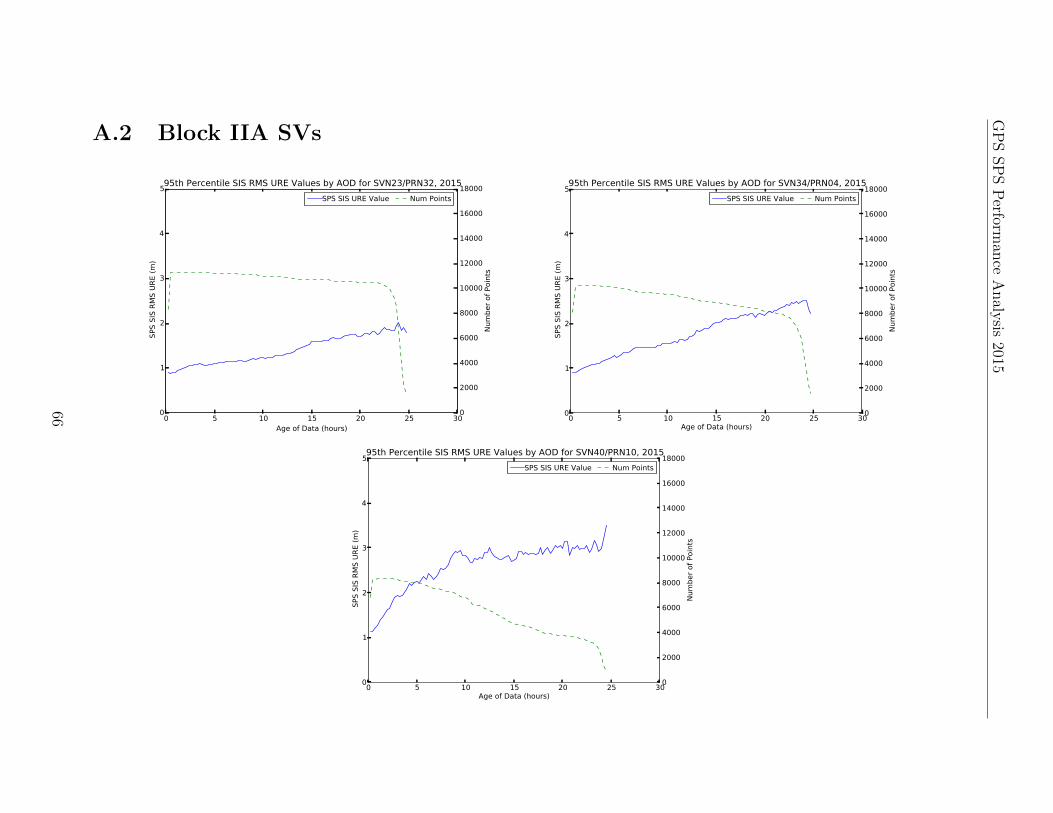
GP
SSP
SP
erforman
ceA
naly
sis2015
A.2 Block IIA SVs
0 5 10 15 20 25 30Age of Data (hours)
0
1
2
3
4
5
SPS
SIS
RM
S UR
E (m
)
0
2000
4000
6000
8000
10000
12000
14000
16000
18000
Num
ber o
f Poi
nts
95th Percentile SIS RMS URE Values by AOD for SVN23/PRN32, 2015SPS SIS URE Value Num Points
0 5 10 15 20 25 30Age of Data (hours)
0
1
2
3
4
5
SPS
SIS
RM
S UR
E (m
)
0
2000
4000
6000
8000
10000
12000
14000
16000
18000
Num
ber o
f Poi
nts
95th Percentile SIS RMS URE Values by AOD for SVN34/PRN04, 2015SPS SIS URE Value Num Points
0 5 10 15 20 25 30Age of Data (hours)
0
1
2
3
4
5
SPS
SIS
RM
S UR
E (m
)
0
2000
4000
6000
8000
10000
12000
14000
16000
18000
Num
ber o
f Poi
nts
95th Percentile SIS RMS URE Values by AOD for SVN40/PRN10, 2015SPS SIS URE Value Num Points
66

GP
SSP
SP
erforman
ceA
naly
sis2015
A.3 Block IIR SVs
0 5 10 15 20 25 30Age of Data (hours)
0
1
2
3
4
5
SPS
SIS
RM
S UR
E (m
)
0
2000
4000
6000
8000
10000
12000
14000
16000
18000
Num
ber o
f Poi
nts
95th Percentile SIS RMS URE Values by AOD for SVN41/PRN14, 2015SPS SIS URE Value Num Points
0 5 10 15 20 25 30Age of Data (hours)
0
1
2
3
4
5
SPS
SIS
RM
S UR
E (m
)
0
2000
4000
6000
8000
10000
12000
14000
16000
18000
Num
ber o
f Poi
nts
95th Percentile SIS RMS URE Values by AOD for SVN43/PRN13, 2015SPS SIS URE Value Num Points
0 5 10 15 20 25 30Age of Data (hours)
0
1
2
3
4
5
SPS
SIS
RM
S UR
E (m
)
0
2000
4000
6000
8000
10000
12000
14000
16000
18000
Num
ber o
f Poi
nts
95th Percentile SIS RMS URE Values by AOD for SVN44/PRN28, 2015SPS SIS URE Value Num Points
0 5 10 15 20 25 30Age of Data (hours)
0
1
2
3
4
5
SPS
SIS
RM
S UR
E (m
)
0
2000
4000
6000
8000
10000
12000
14000
16000
18000
Num
ber o
f Poi
nts
95th Percentile SIS RMS URE Values by AOD for SVN45/PRN21, 2015SPS SIS URE Value Num Points
67

GP
SSP
SP
erforman
ceA
naly
sis20150 5 10 15 20 25 30
Age of Data (hours)0
1
2
3
4
5
SPS
SIS
RM
S UR
E (m
)
0
2000
4000
6000
8000
10000
12000
14000
16000
18000
Num
ber o
f Poi
nts
95th Percentile SIS RMS URE Values by AOD for SVN46/PRN11, 2015SPS SIS URE Value Num Points
0 5 10 15 20 25 30Age of Data (hours)
0
1
2
3
4
5
SPS
SIS
RM
S UR
E (m
)
0
2000
4000
6000
8000
10000
12000
14000
16000
18000
Num
ber o
f Poi
nts
95th Percentile SIS RMS URE Values by AOD for SVN47/PRN22, 2015SPS SIS URE Value Num Points
0 5 10 15 20 25 30Age of Data (hours)
0
1
2
3
4
5
SPS
SIS
RM
S UR
E (m
)
0
2000
4000
6000
8000
10000
12000
14000
16000
18000
Num
ber o
f Poi
nts
95th Percentile SIS RMS URE Values by AOD for SVN51/PRN20, 2015SPS SIS URE Value Num Points
0 5 10 15 20 25 30Age of Data (hours)
0
1
2
3
4
5
SPS
SIS
RM
S UR
E (m
)
0
2000
4000
6000
8000
10000
12000
14000
16000
18000
Num
ber o
f Poi
nts
95th Percentile SIS RMS URE Values by AOD for SVN54/PRN18, 2015SPS SIS URE Value Num Points68

GP
SSP
SP
erforman
ceA
naly
sis20150 5 10 15 20 25 30
Age of Data (hours)0
1
2
3
4
5
SPS
SIS
RM
S UR
E (m
)
0
2000
4000
6000
8000
10000
12000
14000
16000
18000
Num
ber o
f Poi
nts
95th Percentile SIS RMS URE Values by AOD for SVN56/PRN16, 2015SPS SIS URE Value Num Points
0 5 10 15 20 25 30Age of Data (hours)
0
1
2
3
4
5
SPS
SIS
RM
S UR
E (m
)
0
2000
4000
6000
8000
10000
12000
14000
16000
18000
Num
ber o
f Poi
nts
95th Percentile SIS RMS URE Values by AOD for SVN59/PRN19, 2015SPS SIS URE Value Num Points
0 5 10 15 20 25 30Age of Data (hours)
0
1
2
3
4
5
SPS
SIS
RM
S UR
E (m
)
0
2000
4000
6000
8000
10000
12000
14000
16000
18000
Num
ber o
f Poi
nts
95th Percentile SIS RMS URE Values by AOD for SVN60/PRN23, 2015SPS SIS URE Value Num Points
0 5 10 15 20 25 30Age of Data (hours)
0
1
2
3
4
5
SPS
SIS
RM
S UR
E (m
)
0
2000
4000
6000
8000
10000
12000
14000
16000
18000
Num
ber o
f Poi
nts
95th Percentile SIS RMS URE Values by AOD for SVN61/PRN02, 2015SPS SIS URE Value Num Points69

GP
SSP
SP
erforman
ceA
naly
sis2015
A.4 Block IIR-M SVs
0 5 10 15 20 25 30Age of Data (hours)
0
1
2
3
4
5
SPS
SIS
RM
S UR
E (m
)
0
2000
4000
6000
8000
10000
12000
14000
16000
18000
Num
ber o
f Poi
nts
95th Percentile SIS RMS URE Values by AOD for SVN48/PRN07, 2015SPS SIS URE Value Num Points
0 5 10 15 20 25 30Age of Data (hours)
0
1
2
3
4
5
SPS
SIS
RM
S UR
E (m
)
0
2000
4000
6000
8000
10000
12000
14000
16000
18000
Num
ber o
f Poi
nts
95th Percentile SIS RMS URE Values by AOD for SVN50/PRN05, 2015SPS SIS URE Value Num Points
0 5 10 15 20 25 30Age of Data (hours)
0
1
2
3
4
5
SPS
SIS
RM
S UR
E (m
)
0
2000
4000
6000
8000
10000
12000
14000
16000
18000
Num
ber o
f Poi
nts
95th Percentile SIS RMS URE Values by AOD for SVN52/PRN31, 2015SPS SIS URE Value Num Points
0 5 10 15 20 25 30Age of Data (hours)
0
1
2
3
4
5
SPS
SIS
RM
S UR
E (m
)
0
2000
4000
6000
8000
10000
12000
14000
16000
18000
Num
ber o
f Poi
nts
95th Percentile SIS RMS URE Values by AOD for SVN53/PRN17, 2015SPS SIS URE Value Num Points
70
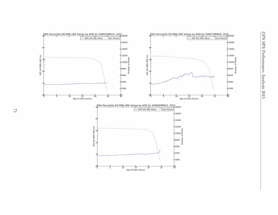
GP
SSP
SP
erforman
ceA
naly
sis20150 5 10 15 20 25 30
Age of Data (hours)0
1
2
3
4
5
SPS
SIS
RM
S UR
E (m
)
0
2000
4000
6000
8000
10000
12000
14000
16000
18000
Num
ber o
f Poi
nts
95th Percentile SIS RMS URE Values by AOD for SVN55/PRN15, 2015SPS SIS URE Value Num Points
0 5 10 15 20 25 30Age of Data (hours)
0
1
2
3
4
5
SPS
SIS
RM
S UR
E (m
)
0
2000
4000
6000
8000
10000
12000
14000
16000
18000
Num
ber o
f Poi
nts
95th Percentile SIS RMS URE Values by AOD for SVN57/PRN29, 2015SPS SIS URE Value Num Points
0 5 10 15 20 25 30Age of Data (hours)
0
1
2
3
4
5
SPS
SIS
RM
S UR
E (m
)
0
2000
4000
6000
8000
10000
12000
14000
16000
18000
Num
ber o
f Poi
nts
95th Percentile SIS RMS URE Values by AOD for SVN58/PRN12, 2015SPS SIS URE Value Num Points71
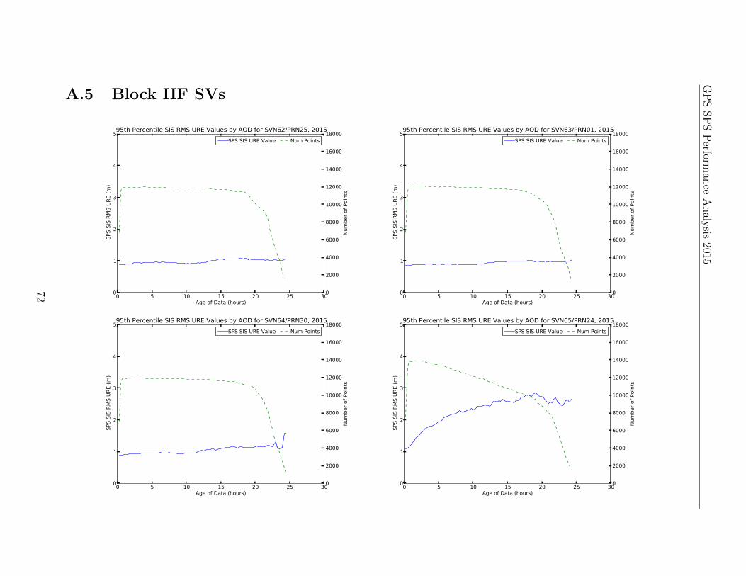
GP
SSP
SP
erforman
ceA
naly
sis2015
A.5 Block IIF SVs
0 5 10 15 20 25 30Age of Data (hours)
0
1
2
3
4
5
SPS
SIS
RM
S UR
E (m
)
0
2000
4000
6000
8000
10000
12000
14000
16000
18000
Num
ber o
f Poi
nts
95th Percentile SIS RMS URE Values by AOD for SVN62/PRN25, 2015SPS SIS URE Value Num Points
0 5 10 15 20 25 30Age of Data (hours)
0
1
2
3
4
5
SPS
SIS
RM
S UR
E (m
)
0
2000
4000
6000
8000
10000
12000
14000
16000
18000
Num
ber o
f Poi
nts
95th Percentile SIS RMS URE Values by AOD for SVN63/PRN01, 2015SPS SIS URE Value Num Points
0 5 10 15 20 25 30Age of Data (hours)
0
1
2
3
4
5
SPS
SIS
RM
S UR
E (m
)
0
2000
4000
6000
8000
10000
12000
14000
16000
18000
Num
ber o
f Poi
nts
95th Percentile SIS RMS URE Values by AOD for SVN64/PRN30, 2015SPS SIS URE Value Num Points
0 5 10 15 20 25 30Age of Data (hours)
0
1
2
3
4
5
SPS
SIS
RM
S UR
E (m
)
0
2000
4000
6000
8000
10000
12000
14000
16000
18000
Num
ber o
f Poi
nts
95th Percentile SIS RMS URE Values by AOD for SVN65/PRN24, 2015SPS SIS URE Value Num Points
72

GP
SSP
SP
erforman
ceA
naly
sis20150 5 10 15 20 25 30
Age of Data (hours)0
1
2
3
4
5
SPS
SIS
RM
S UR
E (m
)
0
2000
4000
6000
8000
10000
12000
14000
16000
18000
Num
ber o
f Poi
nts
95th Percentile SIS RMS URE Values by AOD for SVN66/PRN27, 2015SPS SIS URE Value Num Points
0 5 10 15 20 25 30Age of Data (hours)
0
1
2
3
4
5
SPS
SIS
RM
S UR
E (m
)
0
2000
4000
6000
8000
10000
12000
14000
16000
18000
Num
ber o
f Poi
nts
95th Percentile SIS RMS URE Values by AOD for SVN67/PRN06, 2015SPS SIS URE Value Num Points
0 5 10 15 20 25 30Age of Data (hours)
0
1
2
3
4
5
SPS
SIS
RM
S UR
E (m
)
0
2000
4000
6000
8000
10000
12000
14000
16000
18000
Num
ber o
f Poi
nts
95th Percentile SIS RMS URE Values by AOD for SVN68/PRN09, 2015SPS SIS URE Value Num Points
0 5 10 15 20 25 30Age of Data (hours)
0
1
2
3
4
5
SPS
SIS
RM
S UR
E (m
)
0
2000
4000
6000
8000
10000
12000
14000
16000
18000
Num
ber o
f Poi
nts
95th Percentile SIS RMS URE Values by AOD for SVN69/PRN03, 2015SPS SIS URE Value Num Points73
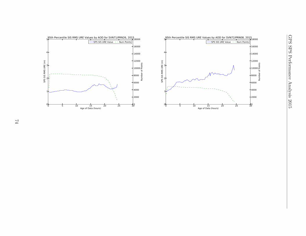
GP
SSP
SP
erforman
ceA
naly
sis20150 5 10 15 20 25 30
Age of Data (hours)0
1
2
3
4
5
SPS
SIS
RM
S UR
E (m
)
0
2000
4000
6000
8000
10000
12000
14000
16000
18000
Num
ber o
f Poi
nts
95th Percentile SIS RMS URE Values by AOD for SVN71/PRN26, 2015SPS SIS URE Value Num Points
0 5 10 15 20 25 30Age of Data (hours)
0
1
2
3
4
5
SPS
SIS
RM
S UR
E (m
)
0
2000
4000
6000
8000
10000
12000
14000
16000
18000
Num
ber o
f Poi
nts
95th Percentile SIS RMS URE Values by AOD for SVN72/PRN08, 2015SPS SIS URE Value Num Points
74

Appendix B
URE Analysis ImplementationDetails
B.1 Introduction
The User Range Error (URE) accuracy represents the accuracy of the broadcastnavigation message. There are a number of error sources that affect the URE, includingerrors in broadcast ephemeris and timing errors.
Two approaches to URE analysis are provided in this report. The first approach usesseparate statistical processes over space and time to arrive at the result. The secondapproach derives the result by a single statistical process but is more computationallydemanding.
B.2 Clock and Position Values for Broadcast and
Truth
The URE values in this report are derived by comparison of the space vehicle (SV)clock and position representations as computed from the broadcast Legacy Navigation(LNAV) message data (BCP) against the SV truth clock and position data (TCP)provided by a precise orbit calculated after the time of interest.
The broadcast LNAV message data used in the calculations were collected by the NGAMSN. These include the complete 300-bit subframes for nearly all unique sets ofsubframe 1, 2, 3 data and all the unique sets of subframe 4, 5 data. The broadcastLNAV messages provide a set of parameters for an equation which can be evaluated atany time for which the parameters are valid. Our process evaluates the parameters ateither a 30 s or 5 min cadence (depending on the process).
The TCP values are computed from the archived National Geospatial-IntelligenceAgency (NGA) products. The archived NGA products used in the calculations are the
75

GPS SPS Performance Analysis 2015
antenna phase center (APC) precise ephemeris files available from the NGA publicwebsite [11]. The NGA products are provided in tabular SP3 format, with positionsand clocks provided at a 5 min cadence. When TCP data are needed at a 5 mincadence, a simple table look-up is sufficient. When TCP data are needed at a 30 scadence, a Lagrange interpolation scheme is used, in which the five points prior to andafter the estimation time are used to estimate the SV position. Clock interpolation ishandled via a linear interpolation since a multipoint Lagrange interpolation is notappropriate for clock dynamics.
B.3 95th Percentile Global Average As Per the SPS
PS
The SPSPS08 specifications for URE suggest averaging across the service volume visibleto a GPS SV at any specified point in time. The process is illustrated in Figure B.1.
Figure B.1: Global Average URE as defined in SPS PS
The equation shown in Figure B.1 is equation A-1 of SPSPS08 Section A.4.11. Thisexpression allows us to compute the URE accuracy from known errors.
For purposes of this report, the Instantaneous RMS SIS URE values were generated at30 s intervals for all of 2015. The URE was formed by differencing the BCP and TCPto obtain the radial, along-track, cross-track, and time errors at each epoch. Theseerrors were used as inputs to the SPSPS08 equation A-1.
76

GPS SPS Performance Analysis 2015
After all the Instantaneous RMS SIS URE values were computed, values for periodswhen each SV was unhealthy or not broadcasting were discarded. The remaining valueswere then grouped by monthly period for each SV and sorted; the maximum and the95th percentile values were identified for each SV, and this is the basis for Table 3.2.The monthly grouping corresponds closely to the 30 day period suggested in theSPSPS08 and PPSPS07 for URE Accuracy over all AODs while being more intuitive tothe reader.
B.4 An Alternate Approach
The previous approach computes an SIS Instantaneous RMS URE (an average overspace) at each time point over a month, then selects a 95th percentile value from thatset. An alternate approach is to compute the SIS Instantaneous URE for a largenumber of locations at each time point and store those results. For each SV, this isdone for a series of time points at a selected cadence, and the collection of SISInstantaneous URE values at each time point are stored. When all the time points for amonth have been computed, the absolute values of SIS Instantaneous URE values forall time points are gathered together in one monthly set. The 95th percentile value isselected from that set.
For this particular implementation, we selected an approximation of an equidistant gridwith a spacing of roughly 550 km (five degrees of latitude on the surface of the Earth).This yields a set of 577 SIS Instantaneous URE values for each SV for each evaluationtime. Figure B.2 illustrates this set of grid points for a particular SV-time shown as aprojection onto the surface of the Earth.
We did this at a cadence of 5 min for each SV for all of 2015 and stored all 577 valuesfor all time points. We then extracted sets of values corresponding to each month(approximately 5 million values per SV-month), took the absolute value of each, andselected the 95th percentile value as the result for the SV-month. This is the basis forTable 3.3.
77

GPS SPS Performance Analysis 2015
Figure B.2: Illustration of the 577 Point Grid
78
GPS SPS Performance Analysis 2015
B.5 Limitations of URE Analysis
There are a number of subtleties in this approach to computing URE accuracies, andthe following paragraphs detail some of these.
Selective Availability (SA) would be an additional significant difference between PPSand SPS results; however, SA was set to zero throughout this period [12].
The approaches described in B.2 - B.4 work well when the estimated URE accuracy isunder the required thresholds, as it verifies that the system is operating as expected.However, experience has shown that when an actual problem arises, the use of thisprocedure, without other cross-check mechanisms, can create some issues and may leadto incorrect results. Consider the following two cases.
• In cases where an SV is removed from service for reasons that invalidate thebroadcast ephemeris (such as a clock run-off) we need to compare the time atwhich the removal from service occurred with the time at which any of the UREaccuracy bounds were exceeded to assess whether or not a violation of the SPSPS metrics occurred. However, because we have relied on the interpolationprocess to generate 30 s values, we cannot obtain an accurate estimate of the timeat which the URE bound was exceeded. As a general rule, the UREs computed inour process should be reviewed when they are contained between two SP3 epochs,one of which contains a clock event.
• When a SV is set unhealthy or cannot be tracked, the precise ephemeris mayprovide misleading results. The analyst preparing the precise ephemeris hasseveral options for handling discontinuities that occur during outages. Therefore,the URE values generated near such events may be incorrect. As a result, it isnecessary to avoid accepting UREs into the statistical process under conditions inwhich the SV could not be tracked or was set unhealthy. This has been done forall the results presented here.
In all cases, when an apparent violation of the URE limits is encountered, we choose toreconcile the analysis described above with the behavior of ORDs formed from the datacollected at NGA and IGS sites. Because the observational data used is collected at a30 s cadence, we obtain a much higher resolution insight into the details of the actualevent than we do with the interpolated PE.
79

Appendix C
SVN to PRN Mapping for 2015
Throughout the report, SVs have been referred to by both SVN and PRN. Keepingtrack of this relationship has become more challenging over the past few years as thenumber of operational SVs is typically very close to the number of available PRNs. Asa result, the relationships have been changing several times throughout a year.Therefore it is useful to have a summary of the PRN to SVN mapping as a function oftime. Figure C.1 presents that mapping for 2015. SVNs on the right vertical axisappear in the order in which they were assigned the PRN values in 2015. Start and endtimes of relationships are indicated by the dates along the upper horizontal axis.
80

GPS SPS Performance Analysis 2015
Fig
ure
C.1
:P
RN
toSV
NM
appin
gfo
r20
15
81

Appendix D
NANU Activity in 2015
Several sections in the report make use of NANUs. It is useful to have a time history ofthe relevant NANUs sorted by SVN. This makes it convenient to determine whichNANU(s) should be examined if an anomaly is observed for a particular satellite at aparticular time.
Figure D.1 presents a plot of the NANU activity in 2015. Green bars are scheduledoutages and red bars represent unscheduled outages. Gray bars represent SVs that havebeen decommissioned. NANU numbers are indicated next to each bar. In the eventthere is more than one NANU for an outage, the last NANU number is displayed.
82
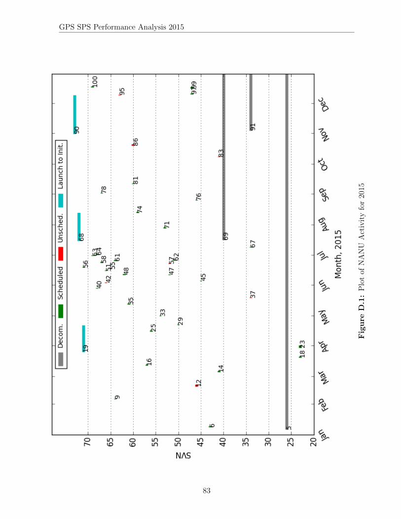
GPS SPS Performance Analysis 2015
Fig
ure
D.1
:P
lot
ofN
AN
UA
ctiv
ity
for
2015
83

Appendix E
SVN to Plane-Slot Mapping for 2015
Several assertions in the PPS PS are related to the performance of the constellation asdefined by the plane-slot arrangement specified in the performance standard.Evaluation of these assertions requires information on the plane-slot occupancy duringthe year.
The operational advisory (OA) provided by 2 SOPS to the United States Coast Guard(USCG) Navigation Center and defined in ICD-GPS-240 includes information onplane-slot assignments. This is a publicly available document and is one of few ways thepublic is informed of slot assignments. However, the format of the OA does not permitit to clearly convey the status of expanded slots. The format is limited to a letterrepresenting the plane and a number representing the slot. There is no provision of the“fore/aft” designation. The OA designations are also cluttered by use of numbersgreater than the number of defined slots. These are “slots of convenience” defined bythe operators but have no fixed meaning in terms of position within the constellation.As a result, interpretation of the OA is challenging.
For the past several years, the plane-slot assignments have been provided to ARL:UTby Aerospace Corporation analysts supporting 2 SOPS. The assignments are providedas a set of daily plane-slot relationships for the year. This information source is notpublicly available.
Both of these sources are limited in that only a single satellite may be designated asbeing present in a slot at a given moment. In fact, as satellites are moved within theconstellation, there exists occasional periods when more than one SV may be presentwithin the defined boundaries of a slot. From the user’s point of view, if a satellitetransmitting a healthy signal is present within the slot boundaries, the slot should becounted as occupied.
ARL:UT has developed a process to independently assess the plane-slot relationships.In what follows, we present an initial independent verification of the plane-slotrelationships.
Figure E.1 provides a graphical illustration of the plane-slot relationships throughout2015. Table E.1 provides the plane-slot relationships in a tabular form. The contents of
84

GPS SPS Performance Analysis 2015
Figure E.1 and Table E.1 are primarily drawn from the information provided byAerospace, cross-checked against the Operational Advisories, and compared with theARL:UT assessment. In the cases where an SV decommissioned or a new SV islaunched, the appropriate NANUs were also checked to confirm dates. In some cases,multiple satellites fall within the slot definition for a period of time. The dates whensatellites are judged to be present in a slot location are noted only when a changeoccurs in the plane-slot during the year. This allows the reader to determine whenmultiple satellites occupied a slot.
Figure E.1 and Table E.1 both indicate that the B1 slot was considered to be anexpanded slot throughout 2015, but only one of the two expanded slot locations wasoccupied until April 2015. Slot B1F became vacant in March 2013 when SVN 35 wasdecommissioned and persisted until SVN 71 became available in April 2015. Theramifications for this are discussed further in Section 3.3 and Section 3.4.
85
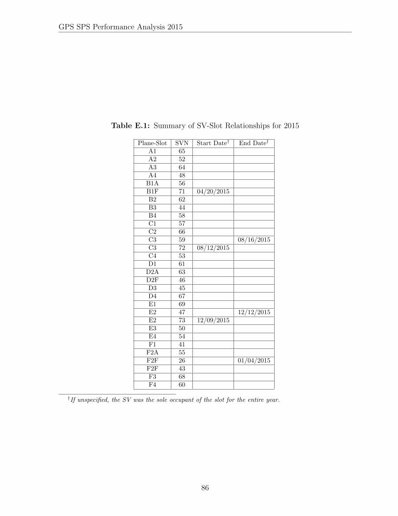
GPS SPS Performance Analysis 2015
Table E.1: Summary of SV-Slot Relationships for 2015
Plane-Slot SVN Start Date† End Date†
A1 65A2 52A3 64A4 48
B1A 56B1F 71 04/20/2015B2 62B3 44B4 58C1 57C2 66C3 59 08/16/2015C3 72 08/12/2015C4 53D1 61
D2A 63D2F 46D3 45D4 67E1 69E2 47 12/12/2015E2 73 12/09/2015E3 50E4 54F1 41
F2A 55F2F 26 01/04/2015F2F 43F3 68F4 60
†If unspecified, the SV was the sole occupant of the slot for the entire year.
86

GPS SPS Performance Analysis 2015
Fig
ure
E.1
:T
ime
His
tory
ofSat
ellite
Pla
ne-
Slo
tsfo
r20
15
87

Appendix F
Translation of URE StatisticsBetween Signals
The URE process described in Appendix B is based on the data broadcast in subframes1, 2, 3 of the navigation message and the NGA PE. Both of these estimates of thesatellite orbits and clock offsets are referenced to the dual-frequency P(Y)-code signal.Therefore, the URE results are directly related to the PPS dual-frequency performance.This appendix explains how these results have been interpreted to apply to the SPSassertions.
The PPS dual-frequency results may be mapped to SPS equivalent results byconsidering the effects of both the group delay differential and the intersignal bias (ISB)between the P(Y)-code and the C/A-Code on L1.
F.1 Group Delay Differential
As described in IS-GPS-200 Section 3.3.1.7, the group delay through the satellitetransmission hardware is accounted for in the satellite clock offset. However, thereremains a group delay differential effect that comes about due to the fact that thesignals passing through the different frequency chains experience slightly differentdelays. An estimate of the group delay differential is transmitted to the users in thenavigation message using the TGD term in Subframe 1. Note that TGD is not the groupdelay differential but the group delay differential scaled to account for the differencebetween a dual-frequency observation and a single-frequency observation. This isdescribed in IS-GPS-200 Section 20.3.3.3.3.2. This distinction will be relevant belowwhen comparisons to other estimates are discussed.
IS-GPS-200 Section 3.3.1.7.2 states that the random plus non-random variations aboutthe mean of the differential delay shall not exceed 3.0 nsec (95% probability). Whilethis establishes an upper bound on the uncertainty, it does not represent actualperformance. The quantization in the TGD term is 0.5 nsec. Therefore, even with
88
GPS SPS Performance Analysis 2015
perfect estimation, the floor on the uncertainty would be on the order of 0.25 nsec.
If one assumes that TGD is correct and that the user equipment properly applies thecorrection, then the single-frequency results would be aligned with the dual-frequencyresults to within that quantization error. However, once the satellite is on orbit it is notpossible to directly observe TGD. Instead it must be estimated, and the estimates aresubject to a variety of factors including receiver group delay differential effects andionospheric dispersion. This uncertainty has the effect of inflating the PPSdual-frequency results when these results are interpreted in terms of the PPSsingle-frequency or SPS services. In fact, because the errors are not directly observable,the best that can be done is to examine the repeatability in the estimate or theagreement between independent estimates and consider these as proxies for the actualuncertainty.
Since 1999, the TGD values have been estimated by Jet Propulsion Laboratory (JPL)and provided to 2 SOPS on a quarterly basis. Shortly before this process was institutedthere was a study of the proposed estimation process and a comparison of the estimatesto those independently developed by two other sources [13]. The day-to-day uncertaintyin the JPL estimates appeared to be about 0.3 nsec and the RMS of the differencesbetween the three processes (after removal of a bias) was between 0.2 nsec and 0.7 nsec.
The Center For Orbit Determination (CODE) at the University of Bern estimates theP1-P2 bias [14]. CODE provides a group delay differential estimate for each SV everymonth. CODE does not provide details on the estimation process, but it must include aconstraint that the group differential delay averaged over the constellation is zero as allsets of monthly values exhibit a zero mean.
A comparison of the CODE estimates and the TGD values (scaled by the groupdifferential delay values) shows a ∼5 nsec bias between the estimates. This bias can beremoved as we are comparing mean-removed vs non-mean removed values. After thebias across the constellation is removed, the level of agreement between the scaled TGD
values and the monthly CODE estimates is between 0.1 nsec and 0.8 nsec RMS. (Note:Results for SVN 49 appear to be out-of-family and have been excluded in thiscomparison)
Considering all these factors, for the purpose of this analysis the uncertainty in the TGD
is assumed to be 0.5 nsec RMS.
F.2 Intersignal Bias
The ISB represents the difference between two signals on the same frequency. This biasis due to differences in the signal generation chain coupled with dispersive effects in thetransmitter due to the differing bandwidths of the signals. It is not possible to observethese effects directly. When examining the signal structure at the nanosecond level thechip edges are not instantaneous transitions with perfectly vertical edges but exhibitrise times that vary by signal. Therefore, measuring the biases requires assumptions
89

GPS SPS Performance Analysis 2015
about the levels at which one decides a transition is in progress. These assumptions willvary between receivers.
There is no estimate of the ISB provided in the GPS legacy navigation message.However, CODE estimates the bias between the L1 P(Y)-code and the L1 C/A-code[14]. An estimate is provided for each SV every month. When this adjustment processwas developed, these estimates were examined for each month in 2013. The monthlymean across all SVs is zero, indicating the estimation process is artificially enforcing aconstraint. The RMS of the monthly values across the constellation is 1.2 nsec for eachmonth. Because there is no estimate of the ISB, this RMS value represents an estimateof the error C/A users experience due to the ISB.
F.3 Adjusting PPS dual-frequency Results for SPS
The PPS dual-frequency and SPS cases are based on a different combination and adifferent code. Therefore, the uncertainties in both TGD and ISB must be considered.The PPS dual-frequency URE results are all stated as 95th percentile (2-sigma) values.This means that the RMS errors estimated in F.1 and F.2 must be multiplied by 1.96(effectively 2, given that the amount of uncertainty in the values).
If it is assumed that these errors are uncorrelated, the total error may be estimated as
Total error =√
((2 ∗ TGD uncertainty)2 + (2 ∗ ISB uncertainty)2)
=√
((2 ∗ 0.5 nsec)2 + (2 ∗ 1.2 nsec)2)
=√
(1 nsec2 + 5.76 nsec2)
= 2.6 nsec
(F.3.1)
Converted to equivalent range at the speed of light and given only a single significantdigit is justified, the total error is about 0.8 m. This adjustment may then be combinedwith the PPS dual-frequency result in a root-sum-square manner.
90

Appendix G
Acronyms and Abbreviations
Table G.1: List of Acronyms and Abbreviations
2 SOPS - 2nd Space Operations Squadron
AMCS - Alternate Master Control Station
AOD - Age of Data
AODO - Age of Data Offset
ARL:UT -Applied Research Laboratories,
The University of Texas at Austin
BCP - Broadcast Clock and Position
CMPS - Civil Monitoring Performance Specification
CODE - Center For Orbit Determination
DECOM - Decommission
DOP - Dilution of Precision
ECEF - Earth-Centered, Earth-Fixed
FAA - Federal Aviation Administration
FCSTDV - Forecast Delta-V
FCSTEXTD - Forecast Extension
FCSTMX - Forecast Maintenance
FCSTRESCD - Forecast Rescheduled
FCSTUUFN - Forecast Unusable Until Further Notice
91

GPS SPS Performance Analysis 2015
GNSS - Global Navigation Satellite System
GPS - Global Positioning System
GPSTK - GPS Toolkit
HDOP - Horizontal Dilution Of Precision
IGS - International GNSS Service
IODC - Issue of Data, Clock
IODE - Issue of Data, Ephemeris
ISB - Intersignal Bias
JPL - Jet Propulsion Laboratory
LSB - Least Significant Bit
MCS - Master Control Station
MSB - Most Significant Bit
MSI - Misleading Signal Information
MSN - Monitor Station Network
NANU - Notice Advisory to Navstar Users
NAV - Navigation Message
NGA - National Geospatial-Intelligence Agency
NMCT - Navigation Message Correction Table
NTE - Not to Exceed
OA - Operational Advisory
ORD - Observed Range Deviation
PDOP - Position Dilution of Precision
PE - Precise Ephemeris
PRN - Pseudo-Random Noise
PVT - Position, Velocity, and Time
RAIM - Receiver Autonomous Integrity Monitoring
RINEX - Receiver Independent Exchange Format
RMS - Root Mean Square
92
GPS SPS Performance Analysis 2015
SA - Selective Availability
SINEX - Station Independent Exchange Format
SIS - Signal-in-Space
SMC/GP - Global Positioning Systems Directorate
SNR - Signal-to-Noise Ratio
SP3 - Standard Product 3
SPS - Standard Positioning Service
SPS PS(SPSPS08) - 2008 Standard Positioning Service Performance Standard
SV - Space Vehicle
SVN - Space Vehicle Number
TCP - Truth Clock and Position
TGD - Group Delay
UNUNOREF - Unusable with No Reference
UNUSUFN - Unusable Until Further Notice
URA - User Range Accuracy
URAE - User Range Acceleration Error
URE - User Range Error
URRE - User Range Rate Error
USCG - United States Coast Guard
USNO - U.S. Naval Observatory
UTC - Coordinated Universal Time
UTCOE - UTC Offset Error
WGS 84 - World Geodetic System 1984
ZAOD - Zero Age of Data
93
Bibliography
[1] U.S. Department of Defense. Standard Positioning Service Performance Standard,4th Edition, 2008.
[2] U.S. Department of Defense. Navstar GPS Space Segment/Navigation UserInterfaces, IS-GPS-200, Revision G, September 2012.
[3] John M. Dow, R.E. Neilan, and C. Rizos. The International GNSS Service in achanging landscape of Global Navigation Satellite Systems. Journal of Geodesy,2009.
[4] B. Renfro, D. Munton, and R. Mach. Around the World for 26 Years - A BriefHistory of the NGA Monitor Station Network. In Proceedings of the Institute ofNavigation International Technical Meeting, Newport Beach, CA, 2012.
[5] U.S.Naval Observatory. Block II Satellite Information.ftp://tycho.usno.navy.mil/pub/gps/gpstd.txt.
[6] W. Gurtner and L. Estey. RINEX: The Receiver Independent Exchange FormatVersion 2.11, 2006.
[7] U.S. Department of Defense. Navstar GPS Control Segment to User SupportCommunity Interfaces, ICD-GPS-240, Revision A, January 2010.
[8] U.S. Department of Transportation. Global Positiong System (GPS) CivilMonitoring Performance Specification, DOT-VNTSC-FAA-09-08, April 2009.
[9] B. Tolman et al. The GPS Toolkit - Open Source GPS Software. In Proceedings ofthe 17th International Technical Meeting of the Satellite Division of the Institute ofNavigation (ION GNSS 2004), Long Beach, CA, 2004.
[10] NIMA Technical Report TR8350.2. Department of Defense World Geodetic System1984, Its Definition and Relationships With Local Geodetic Systems, July 1997.
[11] National Geospatial-Intelligence Agency. NGA Antenna Phase Center PreciseEphemeris products. http://earth-info.nga.mil/GandG/sathtml/ephemeris.html.
[12] The White House, Office of the Press Secretary. Statement by the PresidentRegarding the United States’ Decision to Stop Degrading Global PositioningSystem Accuracy, May 2000.
94

GPS SPS Performance Analysis 2015
[13] Colleen H. Yinger, William A. Feess, Ray Di Esposti, The Aerospace Corporation,Andy Chasko, Barbara Cosentino, Dave Syse, Holloman Air Force Base, BrianWilson, Jet Propulsion Laboratory, Maj. Barbara Wheaton, and SMC/CZUT.GPS Satellite Interfrequency Biases, June 1999.
[14] GPS satellite bias estimates for 2013. ftp://ftp.unibe.ch/aiub/CODE/2013, 2013.
95