An analysis of duration dependence of government revenue ...

HAL Id: halshs-00722083https://halshs.archives-ouvertes.fr/halshs-00722083

Preprint submitted on 31 Jul 2012

HAL is a multi-disciplinary open accessarchive for the deposit and dissemination of sci-entific research documents, whether they are pub-lished or not. The documents may come fromteaching and research institutions in France orabroad, or from public or private research centers.

L’archive ouverte pluridisciplinaire HAL, estdestinée au dépôt et à la diffusion de documentsscientifiques de niveau recherche, publiés ou non,émanant des établissements d’enseignement et derecherche français ou étrangers, des laboratoirespublics ou privés.

An analysis of duration dependence of governmentrevenue expansions and contractions in Developing

CountriesSèna Kimm Gnangnon

To cite this version:Sèna Kimm Gnangnon. An analysis of duration dependence of government revenue expansions andcontractions in Developing Countries. 2012. �halshs-00722083�

https://halshs.archives-ouvertes.fr/halshs-00722083

https://hal.archives-ouvertes.fr

CERDI, Etudes et Documents, E 2012.29

1

C E N T R E D ' E T U D E S

E T D E R E C H E R C H E S

S U R L E D E V E L O P P E M E N T

I N T E R N A T I O N A L

Document de travail de la série

Etudes et Documents

E 2012.29

An analysis of duration dependence of government revenue expansions

and contractions in Developing Countries

Kimm Gnangnon

March 2012

CERDI

65 BD. F. MITTERRAND

63000 CLERMONT FERRAND - FRANCE

TEL. 04 73 17 74 00

FAX 04 73 17 74 28

www.cerdi.org


2

L'auteur

Kimm GNANGNON

PhD student, Clermont Université, Université d’Auvergne, CNRS, UMR 6587, Centre d’Etudes

et de Recherches sur le Développement International (CERDI), F-63009 Clermont-Ferrand,

France

Email : [email protected]

Corresponding author: K. GNANGNON, CERDI-CNRS. Email : [email protected]

La série des Etudes et Documents du CERDI est consultable sur le site :

http://www.cerdi.org/ed

Directeur de la publication : Patrick Plane

Directeur de la rédaction : Catherine Araujo Bonjean

Responsable d’édition : Annie Cohade

ISSN : 2114-7957

Avertissement :

Les commentaires et analyses développés n’engagent que leurs auteurs qui restent seuls

responsables des erreurs et insuffisances.


3

Abstract

In this paper, we employ the discrete-time duration model to examine whether expansion and contraction phases of government revenue exhibit duration dependence. We hence use an unbalanced panel data of public revenue on 68 developing countries over the period 1980-2009. The analysis also covers the sub-samples of sub-Saharan African and Non sub-Saharan African countries. Our findings suggest that once controlling for frailty and economic variables, the likelihood of public revenue expansion and contraction ending appears to be positively affected by their actual age: government revenue expansion and contraction exhibit in developing countries positive duration dependence. Keywords: Government Revenue; Discrete-time model; Duration dependence. JEL Classification: H1; C41 ; H3 ; E6. Acknowledgements I would like to thank M. Jean-François BRUN and M. Gerard CHAMBAS for their helpful comments and suggestions. All errors are the responsibility of the author and the views expressed in this paper are those of the author.


4

1. INTRODUCTION

In today’s world, fiscal policy is more than ever a key development policy tool.

Developing and low-income countries require considerable mobilization of revenue to attain

their development objectives. Many studies have examined the nature of the determinants of

public revenue and their effect on macroeconomic indicators (e.g. for private consumption,

private investment, or economic growth). However, to our knowledge, none of them has

explored the issue of the duration of government revenue cycle phases, namely public revenue

expansion and contraction. The purpose of this paper is to use ‘survival’, ‘duration’ or

‘hazards’ analysis to explore whether public revenue expansion/contraction in developing

countries exhibits duration dependence. This kind of analysis is required to study the length of

time spent by individuals within some state. It models the phenomenon of ‘time to event’ or

‘time failure’, which is also known as ‘spell length’. Duration analysis has often been used in

labour economics to study the duration of periods of unemployment (see for example, Allison,

1982). It has also recently been used to explore issues such as the duration of business cycle

expansions and contractions (see. Castro, 2010), or international trade issues such as the

duration of EU’s imports (Hess et al., 2010).

‘Duration’ in this study refers to the number of years during which government

revenue in a developing country remains either in the expansion or in contraction phases. The

overall goal is to estimate the hazard rate, i.e the probability at which the stay in a given phase

of government revenue cycle (expansion or contraction) ends at time t after a country stays in

that category until t.

This paper explores various key areas of interest. Firstly, we need to determine how

the hazard rate varies with the time spells (duration dependence effect) and with the values of

relevant covariates, having controlled for the heterogeneity that may stem from country

characteristics. Secondly, we will focus both on our full sample of developing countries as

well as on the sub-samples of sub-saharan African countries and non sub-Saharan African

countries, in order to evaluate whether they exhibit different patterns regarding hazard rate

and duration dependence. The hypothesis of state-dependence or path-dependence (see

Eblbers, and Ridder, 1982; Heckman 1991; Parsley and Wei, 1993) implies that repeated

failures in the expansion or contraction of public revenue, especially over a relatively long

period, may build up a positive/negative reputation (i.e it signals some deeply rooted

conditions that are favorable or unfavorable to expansions or contractions). According to


5

Heckman (1981), ‘true state dependence1’ means that the experience of a phase of expansion

or contraction of government revenue in any one year raises the risk of being in the same

phase in the next year. However, rather than indicating true state dependence, the duration

dependence observed in the data may be explained by certain ‘unfavourable’ characteristics

(both observable and unobservable) that justify why certain developing countries leave the

phase of expansion earlier or stay longer in the phase of contraction of government revenue

(this is known as the ‘sorting effect’). Accordingly, the duration of government revenue

phases of expansion/contraction may be unrelated to the hazard rate of government revenue

expansion or contraction. In such cases, the observed relationship between the hazard rate and

the duration of expansions or contractions of government revenue is likely to be spurious and

may indirectly hide other causalities (see also Andriopoulou et al., 2011).

The rest of the paper is organized as follows. Section 2 places the paper in the context of

existing literature. In Section 3, we explain how we date the phases of public revenue cycles,

indicating how we identify peaks and troughs in our dataset. Section 4 outlines the empirical

approach whereas section 5, evaluates the empirical results. Section 6 is the conclusion.

2. LITERATURE REVIEW

The determinants of tax revenues in developing countries have been largely explored in the

empirical literature. The latter broadly encompasses two main strands. The first strand

explores the determinants of tax revenue (or global public revenue) by using cross-section

frameworks and ignoring the variation over time. This includes the work of Lotz and Morss

(1967), Bahl (1971), Chelliah (1971), Chelliah, Baas and Kelly (1975), Tait Eichengreen and

Gratz (1979), Tanzi (1992) and Bird, Martinez-Vasquez and Torgler (2004). The second

strand of the empirical literature introduces the time dimension and includes studies that

examine the determinants of tax revenue over time. Among these works are those of Tanzi

(1981), Leuthold (1991), Stotsky and WoldeMariam (1997), Ghura (1998), Stostky et al.

(2004), Adam, Bevan and Chambas (2001), Gupta (2007), Chambas et al. (2008) and Brun et

al (2011). Most of these studies, in examining the determinants of tax revenues, also construct

a measure of tax effort. Other studies focus more particularly on how tax revenues respond to

1 Precisely, the term «state dependence» is used in order to define the dependence of the status in t on the status

of the dependent variable in t-1, while the term “duration dependence” expresses the dependence of the status in

t on the duration spent in this status. Yet the two terms are often used as synonyms in the literature. In this paper,

we focus on duration dependence but, indirectly, state dependence is also examined.


6

business cycles. For example, Velloso and Xing (2010) have recently examined the

relationship between tax revenue efficiency and the output gap. Their results suggest a

positive and significant effect of these variables, results that are consistent for both advanced

and developing countries and for both quarterly and annual data. In addition, during booms,

the short run elasticity of tax revenue to output is higher than the long-run elasticity,

suggesting that policymakers need to look beyond simple, long-run revenue elasticities and

incorporate into their analysis the effects of the economic cycle on tax revenue efficiency,

particularly during major economic booms and downturns. Gavin and Perotti (1997) also

show evidence that fiscal policy is procyclical in Latin American countries and contracyclical

in industrial countries. More specifically, they find evidence that a one-percentage-point

increase in the rate of output growth in industrial countries is associated with an increase in

the fiscal surplus of about 0.37 percentage points of GDP, whereas the fiscal response in Latin

American countries appears to be negligible (that is, not statistically significant). They also

explore the nature of fiscal policy in Latin America and industrial countries during good and

bad times. Their findings are of two kinds:

-a major asymmetry is found in the fiscal response to output shocks in industrial

countries: during good times, budget surplus increases with GDP growth, whereas the

magnitude of the positive response of fiscal deficit during bad times is higher -

recessions are economically and/or politically more costly than output booms, and the

fiscal policy response to them thus needs to be stronger.

-for Latin American countries, the fiscal balance responds positively and significantly

to a severe decline of real GDP growth (by more than 10%).

Another study of IMF (2005) also finds empirical evidence for the procyclicality of

fiscal policy in advanced, emerging and developing countries. The authors observe evidence

that in emerging and developing countries, a one percentage increase in the output gap is

associated with a deterioration of cyclically-adjusted fiscal balance by 0.5 percentage point of

GDP, whereas the deterioration is of 0.2 percentage point of GDP in advanced countries. In a

similar vein, Kun Li and Pablo Lopez-Murphy (2010) examine how imports affect tax

revenue downturns in advanced, emerging and developing countries. They argue that positive

changes in import-to-GDP ratio are associated with increases in tax revenue-to-GDP ratio.

This result is valid for the different groups of countries (advanced, emerging and developing

countries) used in their study. In addition, for all these groups of countries, there seems to be

no significant response to changes in tax revenues-to-GDP ratio to real GDP growth during


7

bad times. Moreover, an increase in real GDP growth in emerging and developing countries

induces a positive change of tax revenue-to-GDP ratio. This effect is not statistically

significant for advanced economies. This study is influenced by the work of Gavin and Perotti

(1997) and Kun Li and Pablo Lopez-Murphy (2010) and explores whether public revenue

expansions and contractions exhibit duration dependence. In the next section, we explain how

we date the public revenue phases of expansions and contractions.

3. DATING THE PHASES OF PUBLIC REVENUE EXPANSION AND

CONTRACTION IN DEVELOPING COUNTRIES

The identification of specific cycles in economic time series requires precise

definitions of expansion and contraction (Cashin 2004). This applies to government revenues

in developing countries. According to Harding and Pagan (2002), any procedure or algorithm

for extrema identification should follow three fundamental criteria: determining a set of

potential turning points; ensuring alternance between maxima and minima; following a set of

rules that satisfy the pre-determined criteria of duration and magnitude of phases and cycles,

that is, the censoring rules.

The literature on business cycle offers several approaches for identifying the turning

points in ‘classical cycles’. The most frequently one used is that of the NBER, as developed

by Bry and Boschian2 (BB) (1971). His algorithm evolved from the NBER dating of cycles in

U.S. economic activity and has been further adapted by scholars such as King and Plosser

(1994), Watson (1994) and Harding and Pagan (2002a). It is worth mentioning that Pagan

(1999) has also applied the algorithm to date bull and bear markets in equity prices, and

Cashin, McDermott and Scott (2002) have applied it to dating commodity-price cycles.

The empirical literature distinguishes between ‘classical cycles’ and ‘growth cycles’.

The former refers to series in level whereas the latter examines series’ deviations from trends

(Stock and Watson, 1999). Accordingly, the appropriate dating method needs to be chosen,

depending on the objectives the researcher is pursuing.

Cashin (2004), in exploring the key features of Caribbean business cycles during the

annual period 1963-2003, has used a number of criteria for both classical cycles and growth

2 The BB procedure essentially identifies the turning points of high frequency series, generally the monthly data

of GDP, based on the classical definition of cycle proposed by Burns and Mitchell (1946). Other criteria based

on the frequency of the series (the quarterly version of BB’s algorithm) and on Okun’s rule (any contraction

should have a minimum duration of 2 quarters) are also employed (Massmann et al., 2003).


8

cycles to identify peaks and troughs. For the purpose of this study, we will adapt Cashin

(2004)’s method of dating the peaks and troughs of government revenue cycle in developing

countries. In particular, we adopt the ‘classical growth’ method for dating government

revenue expansions and contractions in developing countries for two reasons: firstly, it is the

most appropriate technique for our study and secondly, results based on the ‘growth cycle’

technique are sensitive to the chosen de-trending method (Canova, 1998). We will rely on

these two definitions:

Definition 1: For annual data, an expansion is defined as a sequence of increases in the

government revenue-to-GDP ratio and a contraction, as a sequence of decreases in the

government revenue-to-GDP ratio.

Definition 2: A cycle includes one expansion and one contraction, each of them having

a minimum of one year.

We will follow Cashin and McDermott (2002) and Cashin (2004) in ruling out any

mild interruptions in expansions or contraction. More particularly, we do not consider any

potential change of phase that moves the cycle by less than one half of one per cent per year

as a turning point. The use of ‘classical cycles” leads us to consider expansions/contractions

as periods of absolute rise/decline in the global public revenues-to-GDP ratio, rather than as

periods of below-trend (above-trend) growth in the series (which is the definition of a “growth

cycle”).

Therefore, we can identify the dates of different peaks and troughs for developing

countries’ government revenue-to-GDP ratio phases of expansion and contraction. Our panel

dataset is unbalanced, comprising 68 developing countries (of which 42 are Sub-Saharan

African countries) and covers the period 1980-2009. The choice of that period was dictated by

data availability. For practical reasons, we chose to focus on countries in which the minimum

availability of annual data about government revenue is 26 years. That choice is justified by

the fact that ‘the smaller the samples, the lower are the number of cycles to be identified,

making the results obtained by the identification technique used more sensitive, thus

rendering any statistical inference practically impossible (Abad and Quilis, 1998). Camacho et

al. (2004) also highlight the difficulties in properly identifying the turning points at the

beginning and the end of the period of study, on very small samples, with the possible

consequence of losing important information. In the table 1, we provide standard descriptive

statistics on the duration of expansion/contraction for each country in our sample.


9

It is necessary to point out the importance here of the phenomenon of the ‘censoring’

of spells. Survival analysis which based on spell analysis can suffer from left and right

censoring, meaning that certain spells start before and finish after the period of study. This is

referred to as the left and right censoring status. According to Jenkins (2005), a survival time

is censored if all that is known is that it began or ended within some particular interval of

time, and thus the total spell length (from entry time until transition) is not known exactly.

The right censored spells refers to a spell that does not end within the observation period,

whereas the left-censored ones refer to those that have started prior to the beginning date

(here, the year) of the observation period and for which the exact length is unknown. In

empirical duration analysis, left-censored spells are not taken into account to avoid any

restrictive a priori assumption about the duration dependence of the hazard rate. However,

these right-censored spells do not matter for the derivation of the sample likelihood. This is

why we include in our analysis all right-censored spells, but disregard left-censored spells.

With regard to descriptive statistics tables, in table 1, we report the period of study

(minimum of 26 years and maximum of 30 years), the number of expansions and contractions

spells (where we exclude the spurious points and the left-censoring spells but include the

right-censoring ones), and finally the peaks and troughs. In table 2, we provide the mean, the

standard deviation, the minimum and the maximum duration of the expansion and contraction

of global public revenue-to-GDP ratio. Regarding the latter, the maximum duration of

expansion is 9 years for both the full sample of developing countries and the sub-sample of

sub-Saharan African countries (henceforth referred to as SSA) and 7 years for non sub-

Saharan African countries (henceforth referred to as Non SSA). The maximum duration of

contraction is 8 years for both the full sample of developing countries and the sub-sample of

SSA and 7 years for the sub-sample of Non SSA.

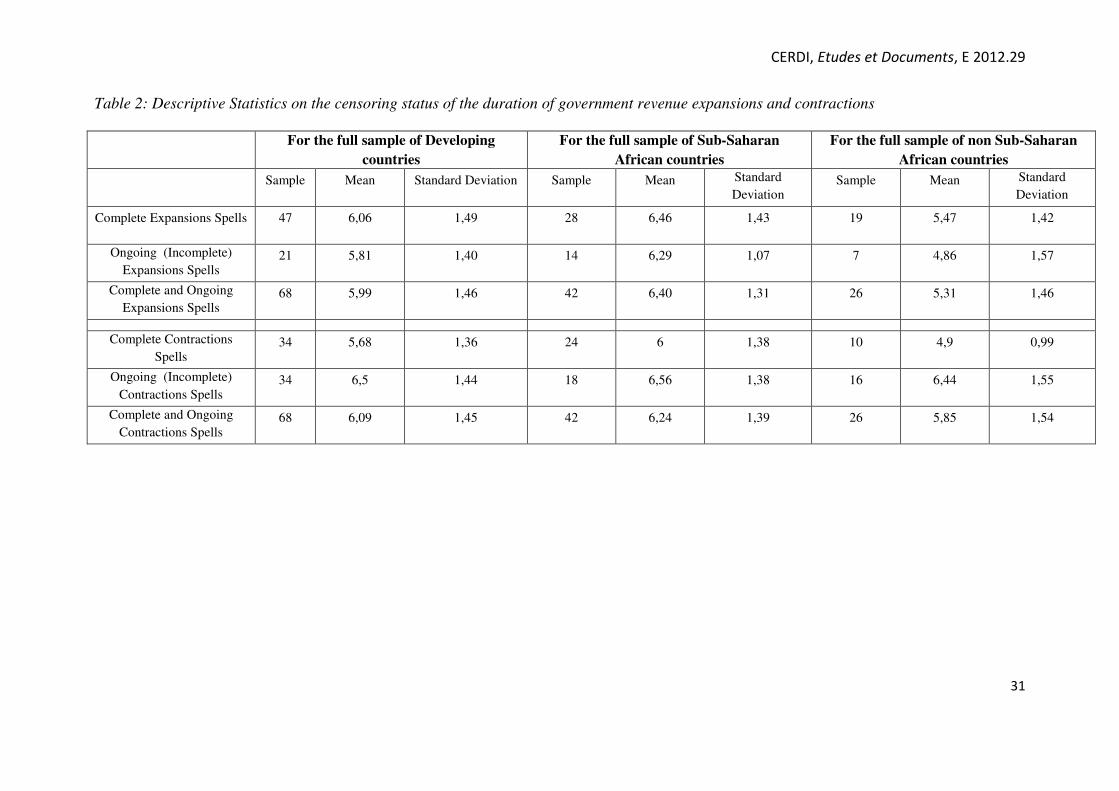
A more thorough descriptive analysis is shown in, table 2, which presents descriptive

statistics for the durations of public revenue expansion/contraction, while making a distinction

between complete and ongoing (incomplete) spells, over the observed period, and figures 1

and 2 plot descriptive survivor functions for the distribution of expansion and contraction

duration. From table 2, it appears that in our dataset, all countries do not exhibit an incomplete

spell of expansion/contraction. In addition, considering the full sample, we can observe that,

on average, complete expansion spells last longer than contraction spells while incomplete

contraction spells last more than incomplete expansion spells. The average length of

expansion duration appears to be higher than that of contraction duration for the sub-samples


10

of SSA and Non SSA. In terms of duration variability, spells of expansions and contraction

display roughly the same standard deviation as the full sample in developing countries, while

the variability of these spells (except complete ones) is higher in Non SSA than in SSA.

In figures 1 and 2, we analyze the survivor function of public revenue expansion and

contraction duration. Hence, we plot the observed spell lengths in the x-axis and the fraction

of observations where the observed spell of expansion/contraction exceeds a given length in

the y-axis. Figure 1 suggests that, in developing countries, approximately 44% of all spells of

expansion cease during the first year and 87% terminate within the first three years, while

52.9% of all contraction spells terminate during the first year and, 94.44% of all contraction

spells end within the first three years. As regards to our two sub-samples, we can observe that

the number of expansions spells that cease during the first year in Sub-Saharan African

countries (47.1%) is higher than that of non Sub-Saharan African countries (37.7%). The

opposite is true for contraction spells (52.29% versus 53.95%). In addition, the number of

expansions spells that terminate within the first three years is higher in SSA (89.96%) than in

non SSA (81.88%), whereas in the case of contraction, an opposite relationship (96.18%

versus 91.45%) can be observed. Therefore, we can conclude that many spells of expansion or

contractions last a few years, while a few are ‘long-lasting’. Thus, the expansion and

contraction of government revenue are often very short-lived.

4. EMPIRICAL APPROACH

4.1 The choice of the model framework: discrete-time or continuous time?

In this section, we lay out the econometric model of the duration of expansions and

contractions of government revenue. In duration models, the key issue is the ‘hazard rate’,

which is the probability of experiencing an event (here, expansions or contractions in

government revenue) after a certain number of years, which is conditional on not having had

experience of the event up to that time. Therefore, in analyzing whether the

expansion/contraction of government revenues in developing countries exhibits duration

dependence patterns, we need to examine whether the probability of public revenue

expansion/contraction duration ending in developing countries depends on the amount of time

spent within that spell. The duration variable is then defined as the number of periods (here,

years) that a country experiences in a state of expansion or contraction, depending on the

phase which is being analyzed. This variable is in our case, continuous. However, the


11

information is available only annually. We have thus grouped (or banded) data and the

discrete hazard model should be used. The adoption of this discrete-time framework is based

on the fact that whereas duration models have initially been conceived in terms of continuous

time-setting, some authors, (e.g. Ohn et al. 2004; Castro 2010, Hess et al., 2011) argue that

discrete-time setting is more appropriate when the minimum duration of phases is a small

multiple of the reference time unit (a quarter) – which is in fact the case here, as we have

annual data. Furthermore, discrete-time duration models have the following advantages:

- they easily allow the inclusion of time-varying covariates within the framework as

well as accounting for unobserved individual heterogeneity, even if the number of

observations is large.

- they can allow us to easily circumvent the restrictive assumptions of proportional

hazards.

Accordingly, in this study, we use parametric discrete-time duration models to

examine whether government revenue in phases of expansion or contraction in developing

countries produces duration dependence. The work of Jenkins (1995, 2005), Castro (2010),

Greene (2003) and Hess et al. (2011) is referenced in relation to this.

One important issue when analyzing discrete-time models is that of spells

independence. In order to obtain consistent parameter estimates from our regression, spells

must be independent. Also, censoring must occur only at interval boundaries, and must not

provide any information about i

T beyond that available in the covariates (see. Hess et al.,

2010; Jenkins, 1995). Hence, to ensure conditional independence between spells, we need to

account for multiple spells as well as for the dependencies existing among

expansions/contractions of government revenue in the same country.

In the next sub-section, we will discuss practical issues related to the implementation

of discrete-time models.

4.2 Discussion of the practical issues related to the implementation of the

discrete-time method

To estimating the hazard rate of a country’s government revenue

expansion/contraction, we are confronted with four main challenges:

- the choice of the covariates entering the model;

- the choice of the functional form of the hazard rate it

P ;

- the choice of the functional form of the baseline hazard rate; and


12

- the choice of whether or not to include unobserved heterogeneity in the model and

if so, the choice of the distribution of that ‘frailty’.

We will now examine each of these challenges.

4.2.1 The first challenge : Choosing the covariates entering the model

The first challenge is to choose the covariates entering the model. In appendices A and

B we provide an overview of all variables, data sources and a list of countries used in our

analysis.

� The dependent variable

To implement our estimation in Stata, as recommended by Jenkins (1995, 2005) for

survival analysis, we need to reorganize our data structure in a person-period format3.

Accordingly, we will create the following variables:

t indicates the time periods the country is at risk or the length of the spell – number of

periods - at which the country experiences government revenue expansion/contraction.

y is a binary dependent variable, which is equal to 1 if the observed spell i ended

during the tth

year, and 0 otherwise. This variable is often referred to as censoring status.

Indeed, as mentioned above (in section 3), we can observe for each spell of government

revenue expansion/contraction, the last year in which it occurs, but not necessary the first year

it has started. Note however that the terminal period may differ across spells (see table 1). In

addition, for the countries that experience several expansions or contractions of government

revenue over the observed period, we have the so called ‘repeated spells’ or ‘multi-failure’

data. These spells may lead to violations of assumptions about homoscedasticity. To obtain

robust standard errors, we need to use inter group correlation for specific countries

� The explanatory variables

We follow Gavin and Perotti (1997)’s model in which changes in fiscal outcomes (in

percent of GDP) are explained by real GDP growth, terms of trade growth, and lagged fiscal

outcomes, and consider the following explanatory variables for our model:

Lagged changes in public revenue (in percent of GDP): the inclusion of this

variable in the model aims at capturing a sort of ‘state-dependence’. We expect an increase of

3 See the easy estimation method of Jenkins (1995) and also Jenkins (2005).


13

the public revenue to-GDP ratio to reduce the likelihood of expansion spells ending, whereas

the opposite effect may be obtained for the probability of contraction spells terminating.

Real GDP growth: this variable is introduced in the model with one year lagged

values to avoid simultaneity problems. The effect of real GDP growth is ambiguous. Indeed,

there is a largely unanimous view among both neoclassical and Keynesian economists, as well

as among policymakers for countercyclical fiscal policies, as optimal fiscal policy. In line

with that view, we expect real GDP growth to reduce the likelihood of government revenue

expansion terminating. However, as the empirical literature demonstrates by providing

evidence of procyclical fiscal policies in developing countries, we may obtain an increase of

the likelihood of expansion ending following a rise in real GDP growth.

At the same time, either approaches suggest that, in good times, government revenue

should increase and that the ratio should decline during bad times. Accordingly, a severe

decline in output during bad times is expected to positively affect the probability of expansion

ending as well as the likelihood of contraction termination. This suggests (with regard to an

unchanged tax base) that public revenue is countercyclical.

Growth rate of terms of trade: An increase of the terms of trade growth rate

following an improvement of terms of trade should reduce the likelihood of the expansion

duration ending and increase the probability of the duration of contraction being terminated.

Number of previous expansions (contractions): We follow the method of Beck et

al., (1998). These authors emphasize that, when dealing with binary time-series cross-section

(BTSC) where the temporal dependence is modeled, ordinary logit or probit models may

result in overly high inferences (t-statistics that are too high). To circumvent that bias, they

suggest adding to the model a variable that picks up the number of previous spells of

expansion or contraction of government revenues. This is in line with our intention to take

into account the repeated nature of spells and thus to conform with the hypothesis that all

spells should be independent and conditional on the covariates. As a result, we include in our

specification the variables ‘numberexpansions’ and ‘numbercontractions’ that capture

respectively the number of previous spells of government revenue expansions and the number

of previous spells of government revenue contractions. We expect that the higher the number

of previous spells of expansions, the lower the likelihood of expansion ending and, the higher

the likelihood of previous contractions spells, the higher the probability of contraction

duration ending. However, we can presume that after a long period of revenue expansion, the

government will, for several reasons, adopt lax tax policies. In the same way, after several


14

periods of public revenue contraction, the government can decide to implement the

appropriate measures to mobilize more revenue, measures which will stop the continuous

period of contraction. Therefore, the expected effects may be the opposite of those mentioned

above.

The baseline hazard rate: The last regressor to be included in our model is the

baseline hazard rate. As explained later, we can model this in the most flexible way by the use

of dummy variables that enable the estimation of period-specific intercepts. Indeed, for spells

of expansion, we can include dummies for each year up to the end of the seventh year (from 1

year to 7 years) and an additional dummy for longer durations (here the maximum spell length

is 9 years, but there is no spell length of 8 years). For spells of contractions that last from 1 to

8 years, we also include dummies for each year up to the eighth year. Additionally, we have

created two dummy variables to capture the effects of the recent financial crisis (that started in

2008): dummy2008 and dummy2009 that take respectively ‘1’ for the years 2008 and 2009

and, ‘0’ otherwise.

4.2.2 The second challenge : The functional form of the baseline hazard rate

The second challenge relates to the choice of the functional form of the hazard rate.

We rely here on Hess et al. (2010). The most commonly encountered functional specifications

(see. Hess et al., 2010) are the normal, logistic, and extreme-value minimum distribution,

leading respectively to probit, logit or cloglog models. The logit and cloglog models are

similar but differ in the fact that a discrete- time hazard model based on a cloglog assumes

proportional hazards, whereas one based on a logit transformation assumes proportional odds

(Singer and Willet 2003; Jenkins 2005). Note that the complementary log-log model can be

interpreted as the discrete time counterpart of an underlying continuous-time proportional

hazard model (see for e.g. Allison, 1982 and Jenkins (1995, 2005). By contrast, the probit

specification is decidedly non-proportional (see also Sueyoski, 1995 for an extensive

discussion of these model specifications in a duration context). In this paper, we implement

the probit, logit and cloglog model and use some criteria described later to choose the model

that fits our dataset better.


15

4.2.3 The third challenge: the choice of the functional form of the

baseline hazard rate.

The third challenge relates to the choice of the functional form of the baseline hazard

rate. According to the literature, several forms of the baseline hazard rate exist (denoting here,

tθ ) : a parametric form of the hazard rate (usually stipulated on the basis of a theoretical

framework – for example the weibull model; a specification linear in time: 0 1ttθ α α= + ; a

polynomial in time: 2

0 1 2 .... ...t t tθ α α α= + + + + ) and a non-parametric method to estimate the

hazard rate (for example piece-wise dummies – one for each particular sub-period of time –

where the hazard rate is assumed to be the same within each time-group but different between

those groups: 0 1 1 2 2 .... ...t

d dθ α α α= + + + + ; or when it is possible, a fully non-parametric

specification with one dummy for each value of t for which the event is reported).

In this paper, as we do not have any theory that dictates the choice of the functional

form of the baseline hazard rate (which characterizes the form of the duration dependence),

we will model it in a flexible way by the use of a piecewise constant specification with a set

of dummy variables for spells of expansions/contractions of government revenues, where the

hazard rate is assumed to be the same within each country-spell but different between those

spells. As the maximum duration of expansion is 9 years and that of contraction 8 years in the

full sample of developing countries, we will proceed to the creation of the dummy variables

as follows: a dummy duration-specific intercept is created for every possible duration from 1

to d_max = 9 for expansions spells and d_max = 8 for contractions spells, where d_max is the

maximum duration. Hence we have, in the absence of a constant in the model, 9 dummy

variables for expansions and 8 dummy variables for contraction; in order to capture the

duration dependence in expansion spells duration and the contraction spells duration.

4.2.4 The fourth challenge : the issue of unobserved heterogeneity

The fourth challenge calls for the choice of whether or not to include ‘unobserved

country specific effects’ or ’frailty’ in the model. If these are included, the choice of the

distribution of unobserved heterogeneity becomes crucial for the ‘frailty’ model. According to

the empirical literature (see Jenkins 2005), ignorance of the heterogeneity effect could lead to

three major biases: an overestimation of negative duration dependence; unstable coefficients

for covariates and biases coefficients for covariates.


16

In the empirical literature, the Gamma and inverse Gaussian distributions are

commonly used for continuous-time model whereas the Gamma Normal (Gaussian)

distributions are used to represent the distribution of unobserved heterogeneity in discrete-

time model. In other words, when estimating discrete-time models, a sensible approach is to

apply conventional binary response panel data models with random effects (see for e.g.

Castro, 2010; Hess et al., 2010; Steele F. A., 2011).

In this paper, we subscribe to the usual convention in estimating discrete-time models and

assuming that the individual-specific unobserved characteristic (unobserved heterogeneity)

follow a log-normal distribution (normally distributed with zero mean and independence of

frailty with all observable characteristics): the individual-specific effects are modeled using

random effects techniques. Hence, by the use of the maximum likelihood method, we estimate

the parameters of the complementary-log-logistic, logit and probit models.

5. EVALUATION OF THE EMPIRICAL RESULTS

In this section, we will discuss the results obtained from the estimation of the baseline

specification of explanatory variables using discrete-time cloglog, logit and probit models

with random effects (In this way we can take account of unobserved individual heterogeneity

or frailty). As mentioned above, the baseline hazard rate is modelled in the most flexible way

by the use of dummy variables that enable the estimation of period-specific intercepts. In

addition, we exclude all left-censored spells which could lead to misestimating the hazard

rate. Given that we have several possible non-parametric models (cloglog, logit and probit

models) we need a rule to discriminate between them in order to interpret our results. The

empirical literature offers us a means to deal with that issue: when non-parametric models are

nested, the likelihood ratio or the wald tests can be used to discriminate between them.

Conversely, when they are not nested, these tests become unsuitable and make it difficult to

choose one model for interpreting our results. In such a situation, a practical and common

approach is to use the Akaike Information Criterion

(AIC): 2(log ) 2( 1)AIC likelihood c q= − + + + where c is the number of model covariates

(explanatory variables) and q is the number of model-specific auxiliary parameters. This

information criterion is proposed by Akaike (1994) and penalizes each log-likelihood to

reflect the number of parameters being estimated in a particular model and then comparing

them.


17

Therefore, the preferred model would be the one with the smallest AIC value (which

describes the data more accurately) despite the fact that the best-fitting model is the one with

the largest log-likelihood. Accordingly, all the choices that will subsequently need to be made

for the interpretation of the model’s results will rely on the Akaike Information Criterion

(AIC).

In tables 4 and 5, we display the results of the estimation of the hazard rate, the latter

picking respectively up the likelihood of termination of government revenue expansion

duration and the likelihood of the termination of government revenue contractions duration. In

these tables, both the duration dependence variables (the dummy variables) and the time-

varying explanatory variables are taken into account and the model uses discrete-time cloglog,

logit and probit models with random effects to conduct estimates.

The results of the duration dependence variables indicate evidence of positive duration

dependence in expansions, except for the spell length of 1 year (see table 3). This means that

in these countries, the likelihood of an expansion ending increases with age. In fact, duration

dependence increases significantly for the spell length ranging from 2 to 5years, and this

become statistically insignificant afterwards. Therefore, the probability of expansion spells

ending increases if the country has experienced an expansion of its public revenue for up to

five periods (years) and the spells that go beyond 5 years do not significantly affect the

likelihood of termination of the government’s revenue expansion . An economic interpretation

of such results may be that, on average, after 5 consecutive years of government revenue

expansion, the governments of these countries need to conduct adequate policy measures

(increasing the tax base and/or tax rate) to avoid the ending of that expansion.

Government revenue contractions (table 4) also exhibit positive duration dependence

from a 2-years spell length until the last spell (8-year spell length). with the exception of a

spell length of 1 year which is not significant in explaining the hazard rate of contraction

termination. This means that, except for the 1 year of spell length, the hazard rate of

government revenue contraction increases with 2 years or more of contraction spells. Hence,

after 1 year of spell length, the governments of these countries take ad-hoc policy measures to

reverse the trend of contractions. Thus, the likelihood of expansions and contractions of

government revenue occurring in these countries becomes more likely to end as years pass.

This means that the likelihood of an expansion ending increases with age. These results

remain valid for the two sub-samples.


18

The results in table 3 reveal that, for both the whole sample of developing countries

and the sub-sample of SSA, the probit model appears to exhibit the smallest AIC criterion.

Accordingly, we will rely on the probit model for interpreting the results stemming from the

different model specifications (columns 3 and 6). The assumption is that the proportional

hazard appears not to be valid for the group of the developing countries and the sub-group of

SSA. However, for the sub-group of non sub-Saharan African countries, the logit model

appears to exhibit the smallest AIC value. The results could thus be interpreted in terms of

proportional log-odds of expansion spells ending and contraction spells terminating. It is

worth mentioning that there is no spell length of 7 years for the sub-sample of SSA (the

maximum spell length is 6 years) and no spell length of 9 years for the Non SSA (the

maximum spell length is 7 years). In table 4, the same AIC criterion suggests the choice of the

probit model whatever group we consider, for the interpretations of our results.

The relative importance of the frailty (unobserved heterogeneity) is given by the

estimates for ρ (rho) displayed in the tables 3 and 4. The “rho” is indeed the ratio of

heterogeneity variance to one plus the heterogeneity variance and in a way this indicates how

much of the model variance is due to unobserved heterogeneity: rho =2

2

( _ )

1 ( _ )

sigma u

sigma u+, where

“sigma_u” is the standard deviation of the unobserved heterogeneity (this is the country-level

random effect standard deviation). If the hypothesis that rho is zero cannot be rejected, then

frailty is unimportant. The p-value of the likelihood ratio test associated with the rho is lower

than 0.01 in all but one cases, suggesting the strong role played by frailty in all but one model

specifications. The only case where the p-value is higher than 10% is that of expansion hazard

rate (column 8 of the table 3) where we retain the logit model.

With regard to the results of the explanatory variables in tables 4 and 5, it is necessary

to take simultaneity problems into account, along with the delay in processing some economic

data. In order to identify their impact on our dependent variable, we include other explanatory

variables with one-year lagged values: the public revenue, as a percentage of GDP; the growth

rate of real GDP; and a dummy capturing bad times, which is calculated on the basis of one-

year lagged values of real GDP growth.

The first regressor is the government revenue as a percentage of GDP. The results,

whatever the sample considered, reveal that the coefficient associated with this variable

presents a negative sign and has a strong power in anticipating the end of expansions and

contractions. In other words, an increase in government revenue (as a percentage of GDP)


19

reduces the likelihood of government revenue expansion ending, whereas a decrease in this

ratio increases the likelihood of the duration contraction termination. The growth rate of the

terms of trade does not affect significantly the likelihood of government revenue expansion

ending. A decrease in the growth rate of real GDP is associated with an increase in the

probability of the expansion ending, whatever the sample considered. This is suggestive of the

countercyclical nature of government revenue during its phases of expansion, if we suppose

the tax base will remain unchanged. In addition, the higher the number of previous spells of

expansion, the lower the likelihood of the expansion terminating. Columns (3), (6) and (9) of

table 4 suggest the following:

- A positive growth rate of terms of trade induces a higher likelihood of contraction

duration ending. This is in the line with our theoretical expectations.

- For the whole sample and the sub-sample of SSA Countries, an increase in the real

GDP growth rate negatively affects the probability of contraction termination. This

means that public revenue will be procyclical during its phases of contractions. For

non SSA countries, the hazard rate of contractions is not significantly associated

with the growth rate of real GDP.

- The number of previous spells appears to exert a negative effect on the likelihood

of government revenue contraction termination for the whole sample of developing

countries, but not for the sub-samples., where the effect is statistically

insignificant.

Does the hazard rate of government revenue expansions/contractions behave differently

during bad times and good times?

The results of table 3 show that the probability of expansion ending is lower in bad

times than in good times, whereas a decline in real GDP growth rate during the bad times

reduces that probability. This reflects a procyclicality of government revenue expansion

phases during bad times, with regard to an unchanged tax base. Furthermore, the probability

of contraction ending also appears to be negatively affected by a decline in real GDP growth

rate during bad times. Phases of revenue contractions appear to be countercyclical (for a fixed

tax base).

In table 4, we can see that the behaviour of the hazard rate of government revenue

contraction is not statistically different in good times and bad times for the sample of all the

developing countries and for the sub-sample of SSA countries but not for non SSA countries,

where the likelihood of contraction terminating is lower in bad times than in good times. By


20

contrast, for the sample of all developing countries and for the sub-sample of SSA countries,

we can find evidence that an increase of the real GDP growth during bad times induces a

higher probability of contraction termination, while a rise in the real GDP growth during bad

times is not significantly associated with the likelihood of a contract ending.

6. CONCLUSION

The literature on government revenue has usually focused either on the determinants of

tax (or total) revenue or on its effects on macroeconomic indicators such as economic growth,

private consumption and investment. This paper departs from the previous by attempting to

explore by introducing hazard analysis in government revenue dynamic analysis. More

particularly, we use an unbalanced panel of public revenue data on 68 developing countries

(of which, 42 sub-Saharan Africans) over the period 1980-2009, to examine whether

government revenue expansion and contraction phases exhibit duration dependence. The

analysis covers both the full sample of developing countries and the sub-samples of sub-

Saharan African and Non sub-Saharan African countries.

The following main conclusions emerge from our study:

• Government revenue expansion and contraction appear to exhibit positive duration

dependence.

• An increase in public revenue in year t compare of that of year t-1 reduces the

probability of government revenue expansion ending and that of contraction

termination.

• Terms of trade growth affects positively and significantly hazard rate of

contraction and does not affect significantly the hazard rate of expansion.

• The expansions of government revenue appear to be countercyclical and the

contractions of government revenue, procyclical, even during bad times.

Summarizing all these results, we conclude that when taking account of frailty, not

only the duration of government revenue expansion and contraction are affected by several

economic variables, but they are also affected by the actual age of expansion and contraction.

Regarding precisely the duration dependence aspect, our analysis suggests interest

results. On the side of contraction, we obtain that the higher the duration of contraction, the

higher its likelihood of ending, suggesting that governments in developing countries, after 1

year of contraction of their public revenue, start finding adequate measures to stop that

contraction trend. By contrast, on the expansion side, the probability of expansion ending


21

increases with the length of the expansion lasting from 2 years to 5 years. However, after 5

years, the effect is statistically insignificant on the hazard rate of expansion. This may suggest

that the governments in developing countries adopt lax tax policies after 1 year and until 5

years of expansion of public revenue.


22

REFERENCE

Allison, Paul D., (1982) “Discrete-time methods for the analysis of event histories”, Sociol

Methodol, vol. 13, pp. 61–98.

Andriopoulou E., and Tsakloglou P., (2011) “The Determinants of Poverty Transitions in

Europe and the Role of Duration Dependence”, IZA DP No. 5692.

Abad, A., et Quilis, E., (1998) “Utilización del bootstrap para caracterizar las propiedades

cíclicas de una serie temporal ”, Instituto Nacional de Estadística (España), boletín trimestral

de coyuntura No 67.

Adam Christopher et al., (2001) “Exchange Rate Regimes and Revenue Performance in Sub-

Saharan Africa,” Journal of Development Economics, Vol. 64, pp. 173–213.

Bahl Roy, (1971) “A Regression Approach to Tax Effort and Tax Ratio Analysis”, IMF Staff

Papers, Vol. 18 (November), pp. 570-612.

Beck Nathaniel et al., (1998) “Taking Time Seriously: Time-Series Cross-Section Analysis

with a Binary Dependent Variable,” American Journal of Political Science, Vol. 42 (October),

pp. 1260–88.

Bird, Richard et al., (2004) “Societal Institutions and Tax Effort in Developing Countries,”

International Studies Program Working Paper 04-06.

Brun Jean-François et al., (2010) ‘IMF programs and tax performance: What role for

institutions in Africa ?’, Working Paper N°33, Centre d’Etudes et de Recherches sur le

Développement International (CERDI).

Brun Jean-François et al., (2008) ‘Aide et mobilisation fiscale dans les pays en

développement’, Working Paper N°12, Centre d’Etudes et de Recherches sur le

Développement International (CERDI).

Burns Arthur F., et al., (1946) “Measuring Business Cycles”, Columbia Univ. Press (New

York: National Bureau of Economic Research).

Camacho, Maximo (2004) ´´Are European Business Cycles Close Enough to be just One?``.

Banco de España.

Canova Fabio, (1998) “Detrending and Business Cycle Facts”, Journal of Monetary

Economics, Vol. 41, No. 3, pp. 475–512.

Cashin, Paul et al., (2002) “Booms and Slumps in World Commodity Prices”, Journal of

Development Economics, No. 69, pp. 277-296.

Cashin Paul, (2004) “Caribbean Business Cycles”, IMF Working Paper WP/04/136.

Castro Victor, (2010) “The duration of economic expansions and recessions: More than

duration dependence”, Journal of Macroeconomics (March 2010), 32 (1), pg. 347-365.


23

Cemile Sancak et al., (2010) “Tax Revenue Response to the Business Cycle”, IMF Working

Paper WP/10/71 (Washington, D.C.: International Monetary Fund).

Chelliah Raja J., (1971) “Trends in Taxation in Developing Countries”, Staff Papers,

International Monetary Fund, Vol. 18, pp. 254–0331.

Chelliah, Raja J., et al., (1975) “Tax Ratios and Tax Effort in Developing Countries, 1969–

71,” Staff papers, International Monetary Fund, Vol. 22, pp. 187–205.

Gavin Michael and Perotti Roberto, (1997) “Fiscal Policy in Latin America,” in NBER

Macroeconomics Annual 1997, ed. by J. Roterberg and B. Bernanke (Cambridge,

Massachusetts: MIT Press).

Ghura Dhaneshwar, (1998) “Tax Revenue in Sub Saharan Africa: Effects of Economic

Policies and Corruption,” IMF Working Paper 98/135 (Washington: International Monetary

Fund).

Greene William., (2003) “Econometric analysis”, 5th ed., Prentice Hall.

Gupta, A., (2007) “Determinants of Tax Revenue Efforts in Developing Countries,” IMF

Working Paper 07/184 (Washington, D.C.: International Monetary Fund).

Harding Don and Pagan Adrian, (2002a) ‘Dissecting the Cycle: A Methodological

Investigation’, Journal of Monetary Economics, No. 49, pp. 365-381.

Heckman James .J., (1981) “Heterogeneity and state dependence”, In: Rosen S (ed) Studies in

labor markets, Chicago Press, Chicago, Illinois.

Heckman, James J. and Singer, B. (1984a) “Econometric duration analysis”, Journal of

Econometrics, vol. 24, pp. 63–132.

Heckman, James J. and Singer, B., (1984b) “A method for minimizing the impact of

distributional assumptions in econometric models for duration data”, Econometrica, vol. 52,

pp. 271–320.

Heckman, James J. (1991) “Identifying the Hand of Past: Distinguishing State Dependence

from Heterogeneity”, Papers and Proceedings of the Hundred and Third Annual Meeting of

the American Economic Association, American Economic Review 81:75-79.

Hess Wolfgang and Persson Maria, (2011) “Exploring the duration of EU imports”, Review

of World Economics, Volume 147, Number 4.

Hess Wolfgang and Persson Maria, (2010) "The Duration of Trade Revisited: Continuous-

Time vs. Discrete-Time Hazards", Working Paper Series 829, Research Institute of Industrial

Economics.

International Monetary Fund, (2005) “Cyclicality of Fiscal Policy and Cyclically Adjusted

Fiscal Balances,” SM/05/393.


24

Jenkins Stephen Pryze, (1995) “Easy estimation methods for discrete-time duration models”,

Oxford B Econ Stat, vol. 57, pp. 129–137.

Jenkins Stephen Pryze, (2005) “Survival analysis”, Unpublished manuscript, Institute for

Social and Economic Research, University of Essex, http:// www.iser.essex.ac.uk/ teaching/

degree/ stephenj/ ec968/ pdfs/ec968lnotesv6.pdf.

Kun Li and Pablo Lopez-Murphy, (2010) “Tax Revenue Downturns: Anatomy and Links to

Imports”, IMF Working Paper WP/10/138.

King Robert and Plosser Charles, (1994) ‘Real Business Cycles and the Test of the

Adelmans’, Journal of Monetary Economics, No. 33, pp. 405-438.

Leuthold, Jane H., (1991) “Tax Shares in Developing Countries: A Panel Study,” Journal of

Development Economics, Vol. 35, pp. 173–185.

Lotz, Jorgen and Morrs Elliott, (1967) “Measuring ‘Tax Effort’ in Developing Countries”,

IMF Staff Papers, Vol. 14, No. 3, pp. 478 - 499.

Massmann, M., Mitchell, J. & Weale, M., (2003) ‘Business cycles and turning points: a

survey of statistical techniques’, National Institute Economic Review 183, 90–106.

Ohn Jonathan et al., (2004) “Testing for duration dependence in economic cycles”,

Econometrics Journal, 7, 528-549.

Pagan Adrian Rodney, (1999) ‘Bulls and Bears: A Tale of Two States’, The Walbow-Bowley

Lecture, presented at the North American Meeting of the Econometric Society, Montreal,

June 1998.

Parsley David and Wei Shang-Jin, (1993) “Insignificant and Inconsequential Hysteresis: The

Case of U.S. Bilateral Trade”, Review of Economics and Statistics 75: 606-13.

Singer Judith D., and Willett John B. (1993) “It’s about time: using discrete-time survival

analysis to study duration and the timing of events”, Journal of Educational Statistics, vol. 18,

pp. 155–195.

Steele Fiona A., (2011) 'Multilevel discrete-time event history analysis with applications to

the analysis of recurrent employment transitions', Australian & New Zealand Journal of

Statistics, 53 (1), (pp. 1-20).

Stock James H., and Watson Mark W., (1999) "Business cycle fluctuations in us

macroeconomic time series, "Handbook of Macroeconomics, in: J. B. Taylor & M. Woodford

(ed.), Handbook of Macroeconomics, edition 1, volume 1, chapter 1, pages 3-64 Elsevier.

Stotsky, Janet G. and WoldeMariam Asegedech, (1997) “Tax Effort in Sub Saharan Africa,”

IMF Working Paper 97/107 (Washington: International Monetary Fund).


25

Tait Alan et al., (1979) “International Comparisons of Taxation for Selected Developing

Countries, 1972–76,” Staff Papers, Vol. 26 (March), pp. 123–156 (Washington, D.C.:

International Monetary Fund).

Tanzi Vito, (1981) “A statistical evaluation of taxation in Sub-Saharan Africa”, Part II in

“Taxation in Sub-Saharan Africa, Occasional Paper No.8, by Fiscal Affairs Department

(Washington: International Monetary Fund).

Tanzi, Vito., (1992) “Structural Factors and Tax Revenue in Developing Countries: A Decade

of Evidence,” in Open Economies: Structural Adjustment and Agriculture, ed. by Ian Goldin

and L. Alan Winters (Cambridge, England: Cambridge University Press), pp. 267–281.

Terence Agbeyegbe et al., (2004) “Trade Liberalization, Exchange Rate Changes, and Tax

Revenue in Sub-Saharan Africa”, IMF Working Paper WP/04/178 (Washington, D.C.:

International Monetary Fund).

Watson Mark W., (1994) ‘Business Cycle Durations and Postwar Stabilization of the U.S.

Economy’, American Economic Review, No. 84, pp. 24-46.


26

Appendix 1: Variables - Definitions and sources

Variable Definition Source Comments

Lagrevenuegdp

The one-year lagged

values of the total

government revenue

(excluding grants),

expressed in

percentage of GDP.

The government revenue data stem from the Public Finance

Database of CERDI (Centre d’Etudes et de Recherches sur le

Developpement International) - France

Author’s calculation of the one-year lagged values of the

total government revenue (excluding grants), expressed in

percentage of GDP.

Growthterms

The growth rate of the

net barters terms of

trade (in percentage

change).

The net barters terms of trade of the World Bank Development

Indicators (2011).

Author’s calculation of the growth rate the net barters terms

of trade.

Lagrealgrowth The one-year lagged

values of the real GDP

growth rate.

The real GDP growth rate data come from the World Bank

Development Indicators (2011).

Author’s calculation of the one-year lagged values of the

real GDP growth rate.

Badtimes

This variable

describes the “bad

times” during the

considered period of

study.

The real GDP growth rate data stem from the World Bank


Author’s calculation: this variable is computed as the years

where one year lagged GDP Growth rate is lower or equal

to "the average of one year Lagged GDP Growth rate less

than one standard deviation".

Badtimesrealgrowth

This variable captures

the value of the one

year lagged real GDP

growth rate during

bad times.

The real GDP growth rate data stem from the World Bank


Author’s calculation: this variable is computed as the

combination of the previously computed variables

“badtimes” and “ realgrowthreta”.


27

Appendix 2: The Different lists of Countries

List of countries of the sample of Developing countries

Argentina, Bahrain, Bangladesh, Belize, Benin, Bhutan, Bolivia, Botswana, Brazil, Burkina Faso, Burundi, Cameroon, Cape Verde, Central

African Republic, Chad, Chile, Colombia, Comoros, Congo Dem. Rep., Congo Rep., Costa Rica, Cote d'Ivoire, Djibouti, Dominican Republic,

Ecuador, Egypt Arab Rep., El Salvador, Ethiopia, Gabon, Gambia, Ghana, Guinea, Guinea-Bissau, Iran, Islamic Rep., Jordan, Kenya, Lesotho,

Madagascar, Malawi, Maldives, Mali, Mauritania, Mauritius, Mexico, Morocco, Mozambique, Namibia, Niger, Nigeria, Pakistan, Peru, Rwanda,

Sao Tome and Principe, Senegal, Sierra Leone, South Africa, Sri Lanka, Sudan, Swaziland, Syrian Arab Republic, Tanzania, Togo, Tunisia,

Turkey, Uganda, Yemen Rep., Zambia, Zimbabwe.

List of countries of the sub-sample of Sub-Saharan African countries

Benin, Botswana, Burkina Faso, Burundi, Cameroon, Cape Verde, Central African Republic, Chad, Comoros, Congo, Dem. Rep., Congo, Rep.,

Cote d'Ivoire, Djibouti, Ethiopia, Gabon, Gambia, Ghana, Guinea, Guinea-Bissau, Kenya, Lesotho, Madagascar, Malawi, Mali, Mauritania,

Mauritius, Mozambique, Namibia, Niger, Nigeria, Rwanda, Sao Tome and Principe, Senegal, Sierra Leone, South Africa, Sudan, Swaziland,

Tanzania, Togo, Uganda, Zambia, Zimbabwe.

Numberexpansions The number of prior

spells of expansions.

Author’s calculation based on the data of Public Finance

Database of CERDI as well as on the criteria used in Cashin

(2004), and described above.

Consider the variable “expansion” that describes for a given

country, the spells of expansions. That variable takes the

value “1” for all expansion’ spells and “0”, otherwise. The

variable “numberexpansions” that captures the number of

previous spells of expansions takes the value “0” for the

first spell and then “1” for the following spell, “2” for the

third spell, and so one…


28

Table 1: Summary Statistics on the distribution of Government Revenue Expansions and Contractions Spells

Country Name Period of Data

Covering

Number of

Expansions'

Spells1

Mean

Expansions

Std Deviation

Expansions

Min

Expansions

Max

Expansions

Number of

Contractions'

Spells1

Mean

Contractions

Std

Deviation

Contractions

Min

Contractions

Max

Contractions

Argentina 1980-2005 5 2.6 1.67332 1 5 4 1.75 .5 1 2

Bahrain 1980-2007 7 1.857143 .6900656 1 3 8 1.625 .5175492 1 2

Bangladesh 1980-2009 5 1.6 .8944272 1 3 6 1.333333 .5163978 1 2

Belize 1980-2009 6 1.833333 .7527727 1 3 7 1.714286 1.112697 1 4

Benin 1980-2009 7 2.142857 1.069045 1 4 6 1.833333 .7527727 1 3

Bhutan 1980-2009 4 3.25 .9574271 2 4 5 1.8 1.30384 1 4

Bolivia 1980-2009 5 3.2 1.30384 2 5 5 1.6 1.341641 1 4

Botswana 1980-2009 8 2 .9258201 1 4 8 1.5 .9258201 1 3

Brazil 1980-2008 6 2.833333 1.834848 1 5 5 1.4 .8944272 1 3

Burkina Faso 1980-2009 7 2.428571 1.397276 1 5 6 1.5 .83666 1 3

Burundi 1980-2009 6 2.166667 1.602082 1 5 7 1.571429 .9759001 1 3

Cameroon 1980-2009 6 1.666667 .8164966 1 3 8 1.75 1.752549 1 6

Cape Verde 1980-2009 7 2.428571 1.511858 1 5 6 1.333333 .8164966 1 3

Central 1980-2009 6 1.5 .5477226 1 2 5 1.8 .83666 1 3

Chad 1980-2009 7 2.285714 1.496026 1 5 5 1.4 .5477226 1 2

Chile 1980-2009 5 2 1.224745 1 4 4 2.5 1.732051 1 5

Colombia 1980-2009 7 2.142857 1.214986 1 4 4 1.25 .5 1 2

Comoros 1980-2008 7 1.428571 .5345225 1 2 8 1.625 .5175492 1 2

Congo, Dem.

Rep. 1980-2009 8 2 1.414214 1 5 6 1.333333 .5163978 1 2

Congo, Rep. 1980-2008 7 2 1.290994 1 4 7 1.285714 .48795 1 2

Costa Rica 1980-2008 5 2.8 1.30384 1 4 4 1.5 1 1 3

Cote d'Ivoire 1980-2009 4 2 .8164966 1 3 5 2.4 2.19089 1 6

Djibouti 1980-2008 5 1.8 .83666 1 3 6 2.5 1.048809 1 4

Dominican 1980-2009 5 3 2.54951 1 7 5 2 .7071068 1 3


29

Ecuador 1980-2007 7 1.714286 .7559289 1 3 6 1.5 .83666 1 3

Egypt, Arab 1980-2009 3 2.333333 .5773503 2 3 6 2.833333 2.857738 1 7

El Salvador 1980-2009 4 3.75 2.217356 1 6 4 2.25 .9574271 1 3

Ethiopia 1980-2009 4 2.25 1.5 1 4 4 3 2.708013 1 7

Gabon 1980-2009 8 1.875 .6408699 1 3 8 1.5 .7559289 1 3

Gambia, The 1980-2009 9 1.333333 .7071068 1 3 9 1.444444 .7264832 1 3

Ghana 1980-2009 9 1.777778 1.092906 1 4 6 1.166667 .4082483 1 2

Guinea 1980-2009 5 2.6 1.81659 1 5 5 2.2 1.643168 1 4

Guinea-Bissau 1980-2009 7 1.571429 .7867958 1 3 6 2.333333 .8164966 1 3

Iran, Islamic 1980-2009 6 2 1.549193 1 5 7 1.714286 1.112697 1 4

Jordan 1980-2009 6 2.333333 1.75119 1 5 7 1.714286 .7559289 1 3

Kenya 1980-2009 6 2 1.264911 2 4 6 1.333333 .8164966 1 3

Lesotho 1980-2009 6 2.833333 .9831921 1 4 4 2 .8164966 1 3

Madagascar 1980-2007 5 2.2 2.167948 1 6 6 1.666667 .5163978 1 2

Malawi 1980-2009 8 1.75 .8864053 1 3 6 1.833333 .4082483 1 2

Maldives 1980-2009 7 2.142857 1.214986 1 4 7 1.428571 .5345225 1 2

Mali 1980-2009 5 2.2 1.643168 1 5 4 2.25 .9574271 1 3

Mauritania 1980-2009 7 1.428571 .5345225 1 2 7 2 .8164966 1 3

Mauritius 1980-2009 5 1.6 .8944272 1 3 6 1.833333 .7527727 1 3

Mexico 1980-2008 2 3 0 3 3 4 3.75 1.707825 2 6

Morocco 1980-2008 5 3.2 1.643168 1 5 5 2.2 1.643168 1 5

Mozambique 1980-2009 5 2.2 1.643168 1 5 6 1.666667 .8164966 1 3

Namibia 1980-2009 8 2 1.511858 1 5 9 1.333333 .7071068 1 3

Niger 1980-2009 5 2.4 1.341641 1 4 5 2 1.732051 1 5

Nigeria 1980-2009 5 2 1 1 3 8 1.5 .7559289 1 3

Pakistan 1980-2009 6 1.666667 .8164966 1 3 10 1.3 .6749486 1 3

Peru 1980-2009 4 3.25 1.258306 2 5 6 1.333333 .5163978 1 2

Rwanda 1980-2009 6 2.666667 1.36626 1 5 5 2 1 1 3

Sao Tome and 1980-2009 8 1.625 .7440238 1 3 7 1.857143 .6900656 1 3

Senegal 1980-2009 7 2 1.414214 1 4 5 2 1 1 3


30

Sierra Leone 1980-2009 6 2.166667 .9831921 1 3 7 1.571429 .5345225 1 2

South Africa 1980-2009 5 2 1 3 6 1.5 .83666 1 3

Sri Lanka 1980-2009 5 1.4 .7071068 1 2 7 2 1.527525 1 5

Sudan 1980-2009 5 2.8 .5477226 1 9 7 1.857143 .8997354 1 3

Swaziland 1980-2009 8 1.5 .7559289 1 3 8 1.75 .8864053 1 3

Syrian Arab 1980-2008 9 1.444444 .8819171 1 3 6 1.5 .5477226 1 2

Tanzania 1980-2009 7 2 1.154701 1 4 5 1.4 .5477226 1 2

Togo 1980-2009 7 1.571429 .7867958 1 3 6 2.5 2.738613 1 8

Tunisia 1980-2009 4 1.5 1 1 3 8 1.875 1.246423 1 4

Turkey 1980-2009 4 4.25 2.217356 2 7 5 2 .7071068 1 3

Uganda 1980-2009 5 3.6 3.286335 1 9 3 1.666667 1.154701 1 3

Yemen, Rep. 1980-2009 6 2 1.095445 1 3 7 2.285714 2.21467 1 7

Zambia 1980-2009 7 1.142857 .3779645 1 2 8 2.125 .834523 1 3

Zimbabwe 1980-2009 6 1.333333 .5163978 1 2 7 2.142857 2.035401 1 6

Note: Standard deviations are in parenthesis - *p-value<0,1; **p-value<0,05; ***p-value<0,01.

1: Spurious points and Left Censoring Spells are excluded.


31

Table 2: Descriptive Statistics on the censoring status of the duration of government revenue expansions and contractions

For the full sample of Developing

countries

For the full sample of Sub-Saharan

African countries

For the full sample of non Sub-Saharan

African countries

Sample Mean Standard Deviation Sample Mean Standard

Deviation Sample Mean Standard

Deviation

Complete Expansions Spells 47 6,06 1,49 28 6,46 1,43 19 5,47 1,42

Ongoing (Incomplete)

Expansions Spells 21 5,81 1,40 14 6,29 1,07 7 4,86 1,57

Complete and Ongoing

Expansions Spells 68 5,99 1,46 42 6,40 1,31 26 5,31 1,46

Complete Contractions

Spells 34 5,68 1,36 24 6 1,38 10 4,9 0,99

Ongoing (Incomplete)

Contractions Spells 34 6,5 1,44 18 6,56 1,38 16 6,44 1,55

Complete and Ongoing

Contractions Spells 68 6,09 1,45 42 6,24 1,39 26 5,85 1,54


32

Figure 1: Descriptive Survivor Functions of government revenue expansions and contractions’ duration in developing countries

Figure 2: Descriptive Survivor Functions of government revenue expansions and contractions’ duration in Sub-Saharan African (SSA) and Non

Sub-Saharan African countries (Non SSA)

Per

cen

tag

e o

f o

bse

rva

tio

ns

wh

ere

the

ob

serv

ed s

pel

ls

exce

ed a

giv

en l

eng

th

Duration of Spells, in Year

Percentage of Expansion_Developing

Countries

Percentage of Contraction_Developing

Countries

Per

cen

tag

e o

f o

bse

rva

tio

ns

wh

ere

the

ob

serv

ed s

pel

ls

exce

ed a

giv

en l

eng

th

Duration of Spells, in Year

Percentage of Expansion_SSA

Percentage of Expansion_nonSSA

Percentage of Contraction_SSA

Percentage of Contraction_nonSSA


33

Table 3: Estimation of the hazard rate of government revenues expansions (Revenue–to-GDP ratio) using the Complementary Log-Logistic

(Cloglog), Logistic and Probit functional forms with random effects.

All Developing Countries Sub-Saharan African Countries Non Sub-Saharan African Countries

RE

Cloglog

RE Logit RE

Probit

RE

Cloglog

RE Logit RE

Probit

RE Cloglog RE Logit RE Probit

Variables

(1) (2) (3) (4) (5) (6) (7) (8) (9) Lagrevenuegdp -0.0685*** -0.0671*** -0.0382*** -0.0684*** -0.0658*** -0.0376*** -0.0737*** -0.0725*** -0.0429***

(0.00899) (0.00915) (0.00520) (0.0108) (0.0110) (0.00618) (0.0170) (0.0174) (0.0104)

Growthterms -0.000124 0.00145 0.00193 0.00364 0.00746 0.00574 -0.00852 -0.00959 -0.00562

(0.00469) (0.00629) (0.00353) (0.00557) (0.00762) (0.00422) (0.00984) (0.0114) (0.00658)

lagrealgrowth -0.0782*** -0.118*** -0.0619*** -0.0748*** -0.111*** -0.0617*** -0.123*** -0.182*** -0.0864***

(0.0224) (0.0283) (0.0155) (0.0259) (0.0330) (0.0182) (0.0445) (0.0577) (0.0309)

Badtimesrealgrowth 0.189** 0.253*** 0.128** 0.237* 0.322** 0.176** 0.204 0.264* 0.123

(0.0846) (0.0974) (0.0501) (0.130) (0.154) (0.0824) (0.126) (0.142) (0.0784)

Badtimes -1.561*** -2.029*** -1.121*** -1.679*** -2.146*** -1.212*** -1.504** -2.057*** -1.090***

(0.368) (0.417) (0.229) (0.449) (0.510) (0.278) (0.646) (0.748) (0.418)

numberexpansions -0.231*** -0.307*** -0.168*** -0.257*** -0.349*** -0.195*** -0.167* -0.192** -0.0963*

(0.0406) (0.0489) (0.0275) (0.0485) (0.0586) (0.0330) (0.0853) (0.0958) (0.0557)

durexp1year 11.20 27.91 10.29 11.72 25.54 10.56 9.168 23.90 8.038

(1050) (12283) (3516) (188.8) (2506) (586.8) (5999) (4565) (433.0)

durexp2year 2.363*** 3.166*** 1.829*** 2.514*** 3.333*** 1.934*** 2.224*** 3.039*** 1.747***

(0.196) (0.248) (0.137) (0.249) (0.311) (0.171) (0.342) (0.450) (0.248)

durexp3year 1.862*** 2.360*** 1.361*** 1.980*** 2.519*** 1.463*** 1.782*** 2.185*** 1.266***

(0.213) (0.252) (0.140) (0.284) (0.331) (0.183) (0.349) (0.422) (0.230)

durexp4year 1.555*** 2.011*** 1.189*** 1.434*** 1.884*** 1.112*** 1.859*** 2.300*** 1.339***

(0.272) (0.317) (0.179) (0.360) (0.417) (0.234) (0.427) (0.487) (0.278)

durexp5year 1.435*** 1.660*** 0.944*** 1.742*** 2.022*** 1.160*** 1.098** 1.235** 0.741**

(0.318) (0.361) (0.202) (0.421) (0.487) (0.276) (0.506) (0.563) (0.304)


34

durexp6year 0.590 0.686 0.466 0.432 0.646 0.430 0.655 0.549 0.478

(0.817) (0.887) (0.494) (1.162) (1.252) (0.697) (1.145) (1.289) (0.693)

durexp7year 0.694 0.694 0.666 0 0 0 0.651 0.616 0.581

(0.820) (0.918) (0.473) (0) (0) (0) (0.840) (0.921) (0.488)

durexp9year -0.209 0.00425 0.112 -0.206 -0.00121 0.108 - - -

(0.825) (0.871) (0.459) (0.841) (0.888) (0.467) - - -

dummy2008 1.170*** 1.747*** 1.002*** 0.676 1.075* 0.681** 2.325*** 2.739*** 1.510***

(0.334) (0.422) (0.224) (0.440) (0.556) (0.294) (0.531) (0.634) (0.362)

dummy2009 1.754*** 1.962*** 1.055*** 2.133*** 2.475*** 1.381*** 0.337 0.290 0.0644

(0.376) (0.463) (0.267) (0.436) (0.554) (0.323) (1.064) (1.160) (0.651)

Observations - Countries 1623-67 1623-67 1623-67 1051-41 1051-41 1051-41 572-26 572-26 572-26

NonZero Outcomes 208 137 71

Log Likelihood -528.96057 -498.56226 -498.07833 -332.55732 -312.67934 -311.10222 -188.06252 -177.83785 -178.83182

Wald Chi2 312.94 309.12 346.26 198.81 195.88 221.11 123.14 124.34 135.70

(0.0000) (0.0000) (0.0000) (0.0000) (0.0000) (0.0000) (0.0000) (0.0000) (0.0000)

AIC 1091.921 1031.125 1030.157 697.1146 657.3587 654.2044 408.125 387.6757 389.6636

sigma_u .8580799 .6599161 .4499451 .8880914 .6939827 .4529634 .6632685 .3729162 .3446748

(.1880346) (.1746644) (.1016043) (.2479229) (.2104713) (.1245927) (.279217) (.3787607) (.1703963)

Rho .3092097 .1168986 .168365 .324085 .1276984 .1702456 .2110095 .0405568 .1061858

(.0936137) (.0546469) (.0632364) (.1223038) (.0675657) (.0777114) (.1401704) (.0790435) (.0938414)

LR associated to Rho 29.12 8.95 16.82 22.38 7.64 11.95 4.93 0.36 2.20

(0.000) (0.001) (0.000) (0.000) (0.003) (0.000) (0.013) (0.274) (0.069)


“-“ means not available.


35

Table 4: Estimation of the hazard rate of Government Revenue Contractions (revenues –to-GDP ratio) using the Complementary Log-Logistic

(Cloglog), Logistic and Probit functional forms with random effects (with control variables).

All Developing Countries Sub-Saharan Africa Countries Non Sub-Saharan African Countries

RE

Cloglog

RE Logit RE

Probit

RE

Cloglog

RE Logit RE

Probit

RE Cloglog RE Logit RE Probit

Variables

(1) (2) (3) (4) (5) (6) (7) (8) (9) Lagrevenuegdp -0.195*** -0.198*** -0.108*** -0.214*** -0.217*** -0.116*** -0.196*** -0.206*** -0.114***

(0.0198) (0.0228) (0.0120) (0.0281) (0.0324) (0.0167) (0.0318) (0.0375) (0.0206)

Growthterms 0.0174*** 0.0199** 0.0107** 0.0143* 0.0171* 0.00955* 0.0293** 0.0326** 0.0163*

(0.00658) (0.00815) (0.00459) (0.00768) (0.00954) (0.00537) (0.0127) (0.0157) (0.00914)

Lagrealgrowth -0.0910*** -0.119*** -0.0615*** -0.110*** -0.138*** -0.0737*** -0.0407 -0.0764 -0.0338

(0.0285) (0.0368) (0.0207) (0.0342) (0.0436) (0.0243) (0.0696) (0.0864) (0.0485)

badtimesrealgrowth 0.112** 0.143** 0.0750* 0.197*** 0.241*** 0.129** -0.0876 -0.103 -0.0710

(0.0547) (0.0716) (0.0396) (0.0724) (0.0936) (0.0530) (0.136) (0.179) (0.100)

badtimes -0.375 -0.503 -0.277 0.0600 0.0881 0.0255 -1.367* -1.934** -1.041*

(0.327) (0.420) (0.237) (0.400) (0.528) (0.298) (0.804) (0.970) (0.541)

numbercontractions -0.118** -0.135* -0.0732* -0.119* -0.138 -0.0820 -0.0517 -0.0243 0.00173

(0.0570) (0.0728) (0.0409) (0.0676) (0.0875) (0.0499) (0.120) (0.147) (0.0819)

durcont1year 19.57 32.13 14.15 21.52 35.87 14.87 13.28 28.17 10.38

(323.4) (5000) (2975) (543.6) (15940) (3214) (373.4) (6934) (778.2)

durcont2year 4.550*** 5.249*** 2.887*** 4.858*** 5.562*** 3.027*** 4.317*** 5.092*** 2.810***

(0.387) (0.448) (0.230) (0.544) (0.623) (0.312) (0.579) (0.692) (0.372)

durcont3year 4.071*** 4.562*** 2.506*** 4.385*** 4.874*** 2.640*** 3.828*** 4.473*** 2.509***

(0.423) (0.485) (0.252) (0.595) (0.671) (0.336) (0.660) (0.798) (0.444)

durcont4year 3.321*** 3.590*** 1.925*** 2.415** 2.571* 1.349* 3.400*** 3.801*** 1.973***

(0.702) (0.802) (0.441) (1.169) (1.340) (0.738) (0.853) (0.987) (0.557)

durcont5year 3.126*** 3.511*** 1.950*** 2.597* 2.512 1.305 3.447*** 4.124*** 2.301***

(0.748) (0.881) (0.473) (1.346) (1.634) (0.884) (0.944) (1.119) (0.631)


36

durcont6year 3.725*** 3.969*** 2.155*** 4.338*** 4.604*** 2.457*** 3.634*** 4.030*** 2.094***

(0.736) (0.836) (0.453) (1.063) (1.248) (0.667) (1.084) (1.209) (0.667)

durcont7year 2.917*** 3.140** 1.669** 2.382* 2.369 1.161 4.432*** 5.072*** 2.724***

(1.085) (1.244) (0.681) (1.443) (1.779) (0.990) (1.542) (1.815) (1.056)

durcont8year 3.381*** 3.435** 1.878** 3.626*** 3.674** 1.929** - - -

(1.271) (1.512) (0.810) (1.362) (1.629) (0.872) - - -

dummy2008 0.965** 1.070* 0.642** 1.092** 1.281* 0.778** 0.627 0.675 0.404

(0.429) (0.558) (0.308) (0.544) (0.715) (0.395) (0.716) (0.923) (0.496)

dummy2009 2.569*** 2.846*** 1.519*** 2.484*** 2.768*** 1.479*** 3.111*** 3.376*** 1.843***

(0.523) (0.635) (0.354) (0.667) (0.806) (0.445) (1.038) (1.210) (0.689)

Observations - Countries 1627-67 1627-67 1627-67 1058-41 1058-41 1051-41 569-26 569-26 569-26

NonZero Outcomes 167 112 55

Log Likelihood -338.55063 -329.66517 -327.37578 -218.82568 -213.08429 -211.39105 -111.91304 -108.77807 -108.65894

Wald Chi2 189.56 182.87 211.84 110.54 106.88 126.96 81.20 76.24 83.66

(0.0000) (0.0000) (0.0000) (0.0000) (0.0000) (0.0000) (0.0000) (0.0000) (0.0000)

AIC 711.1013 693.3303 688.7516 471.6514 460.1686 456.7821 255.8261 249.5561 249.3179

sigma_u 1.473676 1.432029 .8297128 1.661944 1.616547 .8817608 1.118198 1.062284 .7110873

(.2313097) (.2659272) (.1433496) (.3152663) (.3614349) (.1876538) (.3403955) (.4090395) (.2401979)

rho .5690117 .3839861 .4077315 .6267444 .4426873 .4374128 .4318607 .2554023 .3358329

(.0769854) (.0878511) (.0834433) (.088754) (.1103234) (.1047413) (.1493804) (.1464539) (.1506874)

LR associated to Rho 70.77 34.40 40.35 50.92 24.29 27.75 14.18 6.16 8.88

(0.000) (0.000) (0.000) (0.000) (0.000) (0.000) (0.000) (0.007) (0.001)


“-“ means not available.

An analysis of duration dependence of government revenue ...

Documents

Transcript of An analysis of duration dependence of government revenue ...