An Analysis of Cost Overruns and Time Delays of INDOT Projects
191
Final Report FHWA/IN/JTRP-2004/7 An Analysis of Cost Overruns and Time Delays of INDOT Projects by Claire Bordat Graduate Research Assistant Bob G. McCullouch Research Scientist Samuel Labi Visiting Assistant Professor of Civil Engineering and Kumares C. Sinha Olson Distinguished Professor of Civil Engineering School of Civil Engineering Purdue University Joint Transportation Research Program Project No.: C-36-73V File No.: 3-4-22 SPR-2811 Prepared in Cooperation with the Indiana Department of Transportation and the U.S. Department of Transportation Federal Highway Administration The contents of this report reflect the views of the author who is responsible for the facts and the accuracy of the data presented herein. The contents do not necessarily reflect the official views or policies of the Indiana Department of Transportation or the Federal Highway Administration at the time of publication. This report does not constitute a standard, specification, or regulation. Purdue University West Lafayette, Indiana December 2004
Transcript of An Analysis of Cost Overruns and Time Delays of INDOT Projects
Final Report
FHWA/IN/JTRP-2004/7
An Analysis of Cost Overruns and Time Delays of INDOT Projects
by
Claire Bordat Graduate Research Assistant
Bob G. McCullouch Research Scientist
Samuel Labi
Visiting Assistant Professor of Civil Engineering
and
Kumares C. Sinha Olson Distinguished Professor of Civil Engineering
School of Civil Engineering Purdue University
Joint Transportation Research Program
Project No.: C-36-73V File No.: 3-4-22
SPR-2811
Prepared in Cooperation with the Indiana Department of Transportation and the
U.S. Department of Transportation Federal Highway Administration
The contents of this report reflect the views of the author who is responsible for the facts and the accuracy of the data presented herein. The contents do not necessarily reflect the official views or policies of the Indiana Department of Transportation or the Federal Highway Administration at the time of publication. This report does not constitute a standard, specification, or regulation.
Purdue University
West Lafayette, Indiana December 2004
33-1 12/04 JTRP-2004/7 INDOT Division of Research West Lafayette, IN 47906
INDOT Research
TECHNICAL Summary Technology Transfer and Project Implementation Information
TRB Subject Code: 33-1 Construction Control December 2004 Publication No.: FHWA/IN/JTRP-2004/7, SPR-2811 Final Report
An Analysis of Cost Overruns and Time Delays of INDOT Projects
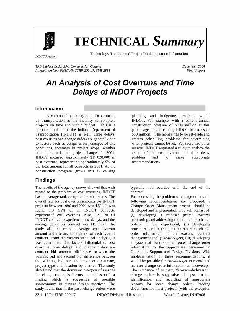
Introduction A commonality among state Departments
of Transportation is the inability to complete projects on time and within budget. This is a chronic problem for the Indiana Department of Transportation (INDOT) as well. Time delays, cost overruns and change orders are generally due to factors such as design errors, unexpected site conditions, increases in project scope, weather conditions, and other project changes. In 2001, INDOT incurred approximately $17,028,000 in cost overruns, representing approximately 9% of the total amount for all contracts in 2001. As the construction program grows this is causing
planning and budgeting problems within INDOT, For example, with a current annual construction program of $700 million at this percentage, this is costing INDOT in excess of $60 million. The money has to be set-aside and creates scheduling problems for determining what projects cannot be let. For these and other reasons, INDOT requested a study to analyze the extent of the cost overrun and time delay problem and to make appropriate recommendations.
Findings The results of the agency survey showed that with regard to the problem of cost overruns, INDOT has an average rank compared to other states. The overall rate for cost overrun amounts for INDOT projects between 1996 and 2001 was 4.5%. It was found that 55% of all INDOT contracts experienced cost overruns. Also, 12% of all INDOT contracts experience time delays, and the average delay per contract was 115 days. The study also determined average cost overrun amount and arte and time delay for each type of contract. From the various statistical analyses, it was determined that factors influential to cost overruns, time delays, and change orders are contract bid amount, difference between the winning bid and second bid, difference between the winning bid and the engineer’s estimate, project type and location by district. The study also found that the dominant category of reasons for change orders is “errors and omissions”, a finding which is suggestive of possible shortcomings in current design practices. The study found that in the past, change orders were
typically not recorded until the end of the contract. For addressing the problem of change orders, the following recommendations are proposed: a Change Order Management process should be developed and implemented. This will consist of: (i) developing a mindset geared towards monitoring and addressing the problem of change orders, in the department, (ii) developing procedures and instructions for recording change order information in the existing contract management tool (SiteManager), (iii) developing a system of controls that routes change order information to the appropriate personnel in Operations Support and Design Divisions. With implementation of these recommendations, it would be possible for SiteManager to record and monitor change order information as it develops. The incidence of so many “no-recorded-reason” change orders is suggestive of lapses in the identification and recording of appropriate reasons for some change orders. Bidding documents for most projects (with the exception
33-1 12/04 JTRP-2004/7 INDOT Division of Research West Lafayette, IN 47906
resurfacing projects) are typically prepared by consultants. A system of instructions and more definitive definitions can help assign appropriate reasons for all change orders and improve documentation. Therefore, a standard report for each consultant and for each contract could be prepared to identify preventive change orders and how such situations may be avoided in future. Moreover, “real time” recording of change orders would likely accelerate the process of feedback to designers and field personnel. If data about change orders is collected on a daily basis, it is possible to create a “weekly change order report” and route it to the appropriate personnel. INDOT personnel should be given ample opportunity to carry out a detailed review of change orders reports and their consequences. Also, such personnel should be encouraged to continually improve their methods. Obviously, implementing additional requirements will be a
challenge, given the current staffing levels and work loads at INDOT. However it is expected that an electronic routing system that collects and distributes change order information would lessen this burden.
It is recommended that INDOT should design an annual report that reviews the performance of consultants. Such a report would assign “grades” to each consultant, taking into account the frequency and dollar amount of preventable change orders that are attributable to the consultant. If grades are to be assigned in such manner, INDOT’s change order classification may be adapted to this new objective in order to better distinguish the responsibilities of each change order type. Finally, INDOT’s current change order classification code can be improved such that an appropriate change order code can be assigned to any situation.
Implementation In evaluating the problem of cost overruns, time delays, and change orders at INDOT, this research effort is consistent with INDOT’s strategic objectives for resource management which include reduction in INDOT overhead costs and increase in the efficiency of the capital program expenditures. The present study provided some initial answers to address problems in the present system. Using the results herein as a starting point, it is possible to carry out future work such as the implementation of a methodology to enhance contract management at INDOT. Another activity is to develop an evaluation procedure to efficiently manage the collection, analysis, and presentation of information on change orders, cost overruns,
and time delays. At the present time, there are indications that INDOT is mulling the establishment a new online system that would directly record change orders from the construction site. The next step would be to enhance the organization of an accompanying database to facilitate monitoring and analysis of change order information and preparation of periodic consultant performance reports. Implementation assistance will be available from Purdue University by contacting the JTRP office or Dr. Bob McCullouch ([email protected], 765-494-0643).
.
Contacts For more information: Dr. Bob G. McCullouch Principal Investigator Purdue University School of Civil Engineering West Lafayette IN 47907 Phone: (765) 494-0643 Fax: (765) 494-0644 E-mail: [email protected] Prof. Kumares C. Sinha Co-Principal Investigator Purdue University School of Civil Engineering West Lafayette IN 47907 Phone: (765) 494-2211 Fax: (765) 496-7996 E-mail: [email protected]
Indiana Department of Transportation Division of Research 1205 Montgomery Street P.O. Box 2279 West Lafayette, IN 47906 Phone: (765) 463-1521 Fax: (765) 497-1665 Purdue University Joint Transportation Research Program School of Civil Engineering West Lafayette, IN 47907-1284 Phone: (765) 494-9310 Fax: (765) 496-7996 E-mail: [email protected] http://www.purdue.edu/jtrp
iiTECHNICAL REPORT STANDARD TITLE PAGE
1. Report No. 2. Government Accession No.
3. Recipient's Catalog No.
FHWA/IN/JTRP-2004/7
4. Title and Subtitle An Analysis of Cost Overruns and Time Delays of INDOT Projects
5. Report Date December 2004
6. Performing Organization Code 7. Author(s) Claire Bordat, Bob G. McCullouch, Samuel Labi, and Kumares C. Sinha
8. Performing Organization Report No. FHWA/IN/JTRP-2004/7
9. Performing Organization Name and Address Joint Transportation Research Program 1284 Civil Engineering Building Purdue University West Lafayette, IN 47907-1284
10. Work Unit No.
11. Contract or Grant No.
SPR-2811 12. Sponsoring Agency Name and Address Indiana Department of Transportation State Office Building 100 North Senate Avenue Indianapolis, IN 46204
13. Type of Report and Period Covered
Final Report
14. Sponsoring Agency Code
15. Supplementary Notes Prepared in cooperation with the Indiana Department of Transportation and Federal Highway Administration. 16. Abstract A commonality among state Departments of Transportation is the inability to complete projects on time and within budget. This project assessed the extent of the problem of cost overruns, time delays, and change orders associated with Indiana Department of Transportation (INDOT) construction projects, identified the reasons for such problems, and finally developed a set of recommendations aimed at their future reduction. For comparison purposes, data from other states were collected and studied using a questionnaire instrument. The analysis of the cost overrun, time delay and change order data was done using an array of statistical methods. The literature review and agency survey showed that time delays, cost overruns and change orders are generally due to factors such as design, unexpected site conditions, increases in project scope, weather conditions, and other project changes. The results of the agency survey showed that with regard to the problem of cost overruns, INDOT has an average rank compared to other states. Between 1996 and 2001, the overall rate for cost overrun amounts for INDOT projects was determined as 4.5%, and it was found that 55% of all INDOT contracts experienced cost overruns. It was determined that the average cost overrun amount and rate, as well as the contributory cost overrun factors differ by project type. The average cost overrun rates were as follows: bridge projects -- 8.1%, road construction -- 5.6%, road resurfacing -- 2.6%, traffic projects -- 5.6%, maintenance projects -- 7.5%. With regard to time delays, it was found that 12% of all INDOT contracts experience time delays, and the average delay per contract was 115 days. With regard to change orders, the study found that the dominant category of reasons for change orders is “errors and omissions”, a finding which is suggestive of possible shortcomings in current design practices The statistical analyses in the present study showed that the major factors of cost overruns, time delays, and change orders in Indiana are contract bid amount, difference between the winning bid and second bid, difference between the winning bid and the engineer’s estimate, project type and location by district. Besides helping to identify or confirm influential factors of cost overruns, time delay and change orders, the developed regression models may be used to estimate the extent of future cost overruns, time delay and change orders of any future project given its project characteristics and any available contract details. Such models can therefore be useful in long-term budgeting and needs assessment studies. Finally, the present study made recommendations for improving the management of projects and the administration of contracts in order to reduce cost overruns, time delays and change orders.
17. Key Words Change orders, cost overruns, time delays, construction delays, liquidated damages, errors and omissions, site conditions.
18. Distribution Statement No restrictions. This document is available to the public through the National Technical Information Service, Springfield, VA 22161
19. Security Classif. (of this report)
Unclassified
20. Security Classif. (of this page)
Unclassified
21. No. of Pages
178
22. Price
Form DOT F 1700.7 (8-69)
iii
TABLE OF CONTENTS
Page
LIST OF TABLES…………………………………………………………………….…. vi LIST OF FIGURES…………………………………………………………………..… viii CHAPTER 1: INTRODUCTION………………………………………………. 1 1.1 Background and Problem Statement……………………………………….. 1 1.2 Objectives of the Study…………………………………………………….. 1 1.3 Study Scope………………………………………………………………… 2 1.4 Study Approach…………………………………………………………….. 2 CHAPTER 2: LITERATURE REVIEW……………………………………… 5 2.1 Introduction………………………………………………………………… 5 2.2 Standard Taxonomy………………………………………………………... 5 2.3 Causes of Time Delays……………………………………………………... 7 2.4 Factors Affecting Cost-Overruns………………………………………….. 10 2.5 Reasons for Change Orders……………………………………………….. 12 2.6 Audit Reports……………………………………………………………… 13 2.7 Discussion of Literature Review…………………………………………... 16 2.8 Chapter Summary…………………………………………………………. 16 CHAPTER 3: AGENCY SURVEY……………………………………………. 18 3.1 Introduction………………………………………………………………... 18 3.2 Cost Overruns and Time Delays: Results of the Agency Survey…………. 18 3.3 Cost and Time Overruns: Comparison among States……………………... 24 3.4 Tracking Change Orders: Comparison among States……………………... 27 3.5 Chapter Summary…………………………………………………………. 28 CHAPTER 4: STUDY METHODOLOGY…………………………………… 29 4.1 Introduction………………………………………………………………... 29 4.2 Descriptive Statistics………………………………………………………. 29 4.3 Statistical Analysis………………………………………………………… 31
4.3.1 Correlation Matrix Analysis………………………………………… 31 4.3.2 Analysis of Variance (ANOVA)……………………………..……... 31 4.3.3 Pair-wise Tests………...…………………………………………….. 32 4.3.4 Graphical Trend Investigation………………..…………………….. 33
4.4 Description of the Modeling Process……………………………………… 33 4.4.1 Response Variables…………………………………………………. 33
4.4.1.1 Cost Overrun…………………………………………………... 34 4.4.1.2 Time Delay…………………………………………………….. 34 4.4.1.3 Change Orders………………………………………………… 34
4.4.2 Independent Variables……………………………………………... 34
iv
4.4.3 Project Types………………………………………………………. 37 4.4.4 Investigation and Selection of Functional Forms………………….. 37 4.4.5 Model Calibration and Validation…………………………………. 37
4.5 Chapter Summary…………………………………………………………. 38 CHAPTER 5: DATA COLLECTION……………………………………….. 39 5.1 Introduction………………………………………………………………... 39 5.2 Data Collection……………………………………………………………. 39
5.2.1 INDOT Information……………………………………………….. 39 5.2.2 Weather Data……………………………………………………… 42
5.3 Database Development……………………………………………………. 42 5.3.1 Refinement of the Dataset…………………………………………. 42 5.3.2 Weather Database……………………………..………………….. 42 5.3.3 Construction of the Database……………………………………… 44
5.4 Chapter Summary…………………………………………………………. 45 CHAPTER 6: DESCRIPTIVE STATISTICS………………………………... 46 6.1 Introduction………………………………………………………………... 46 6.2 General Description……………………………………………………….. 46
6.2.1 Distribution of Contracts by District……………………………... 46 6.2.2 Distribution of Contracts by Project Type………………………... 47
6.3 Time Overruns…………………………………………………………….. 47 6.3.1 Analysis of Liquidated Damages…………………………………. 47 6.3.2 Analysis of Time Delays………………………………………….. 49
6.4 Cost Overruns and Underruns…………………………………………….. 53 6.4.1 Cost Underruns…………………………………………………… 54 6.4.2 Cost Overruns…………………………………………………….. 60
6.5 Change Orders……………………………………………………………. 61 6.5.1 General Description of the Change Orders………………………. 63 6.5.2 Reasons for Change Orders………………………………………. 65
6.6 Chapter Summary……………………………………………………….. 82 CHAPTER 7: STATISTICAL ANALYSIS PART I………………………….. 83 7.1 Introduction……………………………………………………………… 83 7.2 Correlation Matrix……………………………………………………….. 83 7.3 Analysis of Variance (ANOVA)…………………………………………. 84 7.4 Pair-wise t-Tests………………………………………………………….. 86
7.4.1 “Bid Amount” Pairs……………………………………………. 86 7.4.2 “Duration” Pairs……………………………………………….. 87 7.4.3 “Proportion of Inclement Weather Days” Pairs……………….. 87 7.4.4 “Level of Competition” Pairs………………………………….. 87 7.4.5 “Proportion of the Difference between the Winning and Second
Bid” Pairs…………. 88 7.4.6 “Proportion of the Difference between the Bid and the Engineer’s Estimate” Pairs………. 88 7.4.7 Pair-wise t-Test Conclusions……………………...…………… 88
7.5 Preliminary Graphical Analysis of the Influence of Independent Variables on the Dependent Variables……………………………………………… 89
7.5.1 Cost Overrun…………………………………………………… 89 7.5.2 Time Overrun…………………………………………………... 92
v
7.5.3 Number of Change Orders……………………………………... 95 7.5.4 Conclusion of the Graphical Analysis………………………..... 97 7.6 Chapter Summary………………………………………………………... 98 CHAPTER 8: STATISTICAL ANALYSIS PART II (MODELING)………. 99 8.1 Introduction……………………………………………………………… 99 8.2 Models for Change Orders………………………………………………. 101 8.2.1 Models that Estimate the Frequency of Change Orders…………. 101 8.2.1.1 Frequency of Change Orders for All Project Types Combined … 101
8.2.1.2 Frequency of Change Orders for Bridge Projects………………. 102 8.2.1.3 Frequency of Change Orders for Maintenance Projects……….… 103 8.2.1.4 Frequency of Change Orders for Road Construction Projects….. 104 8.2.1.5 Frequency of Change Orders for Traffic Projects………………. 105 8.2.1.6 Frequency of Change Orders for Resurfacing Projects……….. 107
8.2.2 Models that Estimate Change Order Amount……………………………. 107 8.3 Models for Estimating Time Delay…………………………………….. 109 8.3.1 Time Delay for All Project Types Combined………………….. 109 8.3.2 Time Delay for Bridge Projects………………………………... 110 8.3.3 Time Delay for Maintenance Projects…………………………. 111 8.3.4 Time Delay for Road Construction Projects…………………… 112 8.3.5 Time Delay for Traffic Projects………………………………... 113 8.3.6 Time Delay for Resurfacing Projects………………………….. 113 8.3.7 Discussion for Time Delay Models……………………………. 114
8.4 Models for Estimating Cost Overruns……………………… 115 8.4.1 Estimation of Cost Overrun Amounts…………………………….. 115 8.4.1.1 Cost Overrun Amounts All Project Types Combined…….. 115 8.4.1.2 Cost Overrun Amounts for Bridge Projects………….……. 116 8.4.1.3 Cost Overrun Amounts for Maintenance Projects…….…... 117 8.4.1.4 Cost Overrun Amounts for Road Construction Projects…... 117 8.1.4.5 Cost Overrun Amounts for Traffic Projects………………. 118 8.1.4.6 Cost Overrun Amounts for Resurfacing Projects………… 118 8.4.2 Cost Overrun Rate……………………………………………….… 120
8.5 Chapter Discussion………………………………………… 120 8.6 Chapter Summary………………………………………… 122
CHAPTER 9: CONCLUSIONS………………………………………………. 123 CHAPTER 10: RECOMMENDATIONS…………………………………… 126 CHAPTER 11: IMPLEMENTATION……………………………………….. 128 CHAPTER 12: REFERENCES………………………………………………. 129 APPENDIX A: E-MAIL SOLICITATION LETTER TO AGENCIES …… 131 APPENDIX B: INDOT’S CHANGE ORDER ORGANIZATION……….. 132 APPENDIX C: CHANGE ORDER CLASSIFICATION AT STATE DOTS 135 APPENDIX D: WEATHER DATA ORGANIZATION…………….……. 142
vi
APPENDIX E: DESCRIPTIVE STATISTICS……………………….... 144 APPENDIX F: STATISTICAL ANALYSIS………………………........ 163 APPENDIX G: ARIZONA DOT MANAGEMENT OF COST
AND TIME OVERRUN………………………… 177
vi
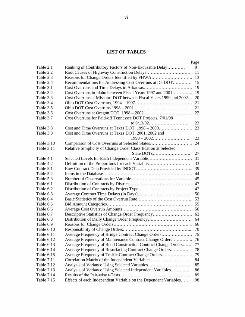
LIST OF TABLES
Page Table 2.1 Ranking of Contributory Factors of Non-Excusable Delay………… 9 Table 2.2 Root Causes of Highway Construction Delays………………………….. 11 Table 2.3 Reasons for Change Orders Identified by FHWA………………………. 13 Table 2.4 Recommendations for Addressing Cost Overruns at DelDOT………….. 15 Table 3.1 Cost Overruns and Time Delays in Arkansas…………………………… 19 Table 3.2 Cost Overruns in Idaho between Fiscal Years 1997 and 2001………….. 19 Table 3.3 Cost Overruns at Missouri DOT between Fiscal Years 1999 and 2002… 20 Table 3.4 Ohio DOT Cost Overruns, 1994 – 1997………………………………… 21 Table 3.5 Ohio DOT Cost Overruns 1998 – 2001…………………………………. 21 Table 3.6 Cost Overruns at Oregon DOT, 1998 – 2002…………………………… 22 Table 3.7 Cost Overruns for Paid-off Tennessee DOT Projects, 7/01/98 to 9/13/02………………………. 23 Table 3.8 Cost and Time Overruns at Texas DOT, 1998 – 2000………………….. 23 Table 3.9 Cost and Time Overruns at Texas DOT, 2001, 2002 and 1998 – 2002……………………. 23 Table 3.10 Comparison of Cost Overruns at Selected States……………………….. 24 Table 3.11 Relative Simplicity of Change Order Classification at Selected State DOTs………………….…. 27 Table 4.1 Selected Levels for Each Independent Variable………………………… 31 Table 4.2 Definition of the Proportions for each Variable………………………… 33 Table 5.1 Raw Contract Data Provided by INDOT…………………………….….. 39 Table 5.2 Items in the Database……………………………………………………. 44 Table 5.3 Number of Observations for Variable…………………………………… 45 Table 6.1 Distribution of Contracts by District…………………………………….. 47 Table 6.2 Distribution of Contracts by Project Type………………………………. 47 Table 6.3 Average Contract Time Delays (in Days)………………………………. 50 Table 6.4 Basic Statistics of the Cost Overrun Rate………………………………. 53 Table 6.5 Bid Amount Categories…………………………………………………. 55 Table 6.6 Average Cost Overrun Amounts………………………………………… 56 Table 6.7 Descriptive Statistics of Change Order Frequency……………………… 63 Table 6.8 Distribution of Daily Change Order Frequency………………………… 64 Table 6.9 Reasons for Change Orders……………………………………………... 66 Table 6.10 Responsibility of Change Orders……………………………………….. 70 Table 6.11 Average Frequency of Bridge Contract Change Orders………………… 75 Table 6.12 Average Frequency of Maintenance Contract Change Orders………….. 76 Table 6.13 Average Frequency of Road Construction Contract Change Orders……. 77 Table 6.14 Average Frequency of Resurfacing Contract Change Orders…………... 78 Table 6.15 Average Frequency of Traffic Contract Change Orders………………… 79 Table 7.11 Correlation Matrix of the Independent Variables……………………… 84 Table 7.12 Analysis of Variance Using Selected Variables……………………….. 85 Table 7.13 Analysis of Variance Using Selected Independent Variables…………. 86 Table 7.14 Results of the Pair-wise t-Tests………………………………………… 89 Table 7.15 Effects of each Independent Variable on the Dependent Variables…… 98
vii
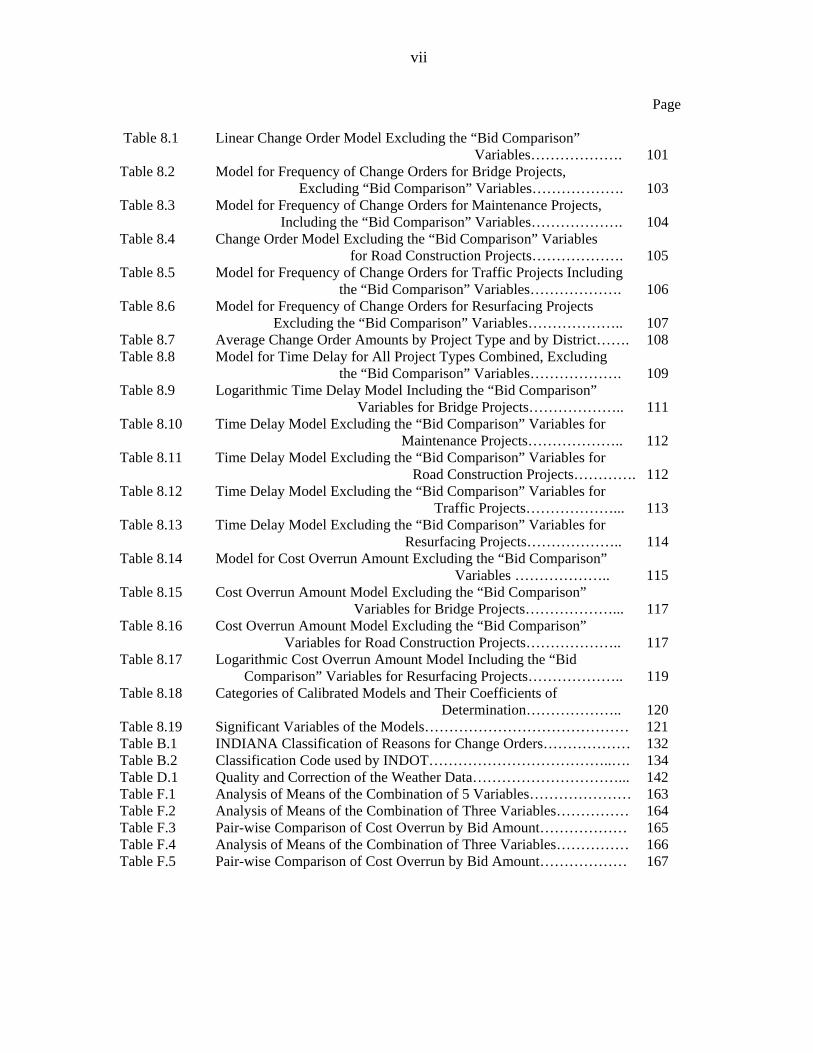
Page Table 8.1 Linear Change Order Model Excluding the “Bid Comparison” Variables………………. 101 Table 8.2 Model for Frequency of Change Orders for Bridge Projects, Excluding “Bid Comparison” Variables………………. 103 Table 8.3 Model for Frequency of Change Orders for Maintenance Projects, Including the “Bid Comparison” Variables………………. 104 Table 8.4 Change Order Model Excluding the “Bid Comparison” Variables for Road Construction Projects………………. 105 Table 8.5 Model for Frequency of Change Orders for Traffic Projects Including the “Bid Comparison” Variables………………. 106 Table 8.6 Model for Frequency of Change Orders for Resurfacing Projects Excluding the “Bid Comparison” Variables……………….. 107 Table 8.7 Average Change Order Amounts by Project Type and by District……. 108 Table 8.8 Model for Time Delay for All Project Types Combined, Excluding the “Bid Comparison” Variables………………. 109 Table 8.9 Logarithmic Time Delay Model Including the “Bid Comparison” Variables for Bridge Projects……………….. 111 Table 8.10 Time Delay Model Excluding the “Bid Comparison” Variables for Maintenance Projects……………….. 112 Table 8.11 Time Delay Model Excluding the “Bid Comparison” Variables for
Road Construction Projects…………. 112 Table 8.12 Time Delay Model Excluding the “Bid Comparison” Variables for Traffic Projects………………... 113 Table 8.13 Time Delay Model Excluding the “Bid Comparison” Variables for Resurfacing Projects……………….. 114 Table 8.14 Model for Cost Overrun Amount Excluding the “Bid Comparison”
Variables ……………….. 115 Table 8.15 Cost Overrun Amount Model Excluding the “Bid Comparison” Variables for Bridge Projects………………... 117 Table 8.16 Cost Overrun Amount Model Excluding the “Bid Comparison” Variables for Road Construction Projects……………….. 117 Table 8.17 Logarithmic Cost Overrun Amount Model Including the “Bid Comparison” Variables for Resurfacing Projects……………….. 119 Table 8.18 Categories of Calibrated Models and Their Coefficients of Determination……………….. 120 Table 8.19 Significant Variables of the Models…………………………………… 121 Table B.1 INDIANA Classification of Reasons for Change Orders……………… 132 Table B.2 Classification Code used by INDOT………………………………..…. 134 Table D.1 Quality and Correction of the Weather Data…………………………... 142 Table F.1 Analysis of Means of the Combination of 5 Variables………………… 163 Table F.2 Analysis of Means of the Combination of Three Variables…………… 164 Table F.3 Pair-wise Comparison of Cost Overrun by Bid Amount……………… 165 Table F.4 Analysis of Means of the Combination of Three Variables…………… 166 Table F.5 Pair-wise Comparison of Cost Overrun by Bid Amount……………… 167
vi
Page Table F.6 Pair-wise Comparison of Time Delay by Bid Amount………………….. 168 Table F.7 air-wise Comparison of Number of Change Orders by Bid Amount…… 169 Table F.8 Pair-wise Comparison of Time Delay by Duration……………………… 169 Table F.9 Pair-wise Comparison of Cost Overrun by Proportion of Inclement
Weather Days…………………………. 170 Table F.10 Pair-wise Comparison of Time Delay by Proportion of Inclement
Weather Days…………………………. 171 Table F.11 Pair-wise Comparison of Cost Overrun by Level of Competition………. 172 Table F.12 Pair-wise Comparison of Number of Change Orders by Level of
Competition…………………………… 173 Table F.13 Pair-wise Comparison of Cost Overrun by Proportion of the Difference
between the First and Second Bid……………… 174 Table F.14 Pair-wise Comparison of Time Delay by Proportion of the Difference
between the First and Second Bid……………… 175 Table F.15 Pair-wise Comparison of Cost Overrun by Proportion of the Difference
between the Bid and the Engineer’s Estimate… 176
viii
LIST OF FIGURES Page
Figure 1.1 Overall Study Approach………………………………………………. 3 Figure 2.1 Contributory Factors of Non-Excusable Delay (Majid and McCaffer, 1998)…………………….. 8 Figure 2.2 Relationship between Literature Review and Other Aspects of the Study………………………………………... 17 Figure 3.1 Yearly Distribution of Cost Overruns at Selected States………………... 25 Figure 3.2 Average Annual Amount of Cost Overruns at Selected States………….. 25 Figure 3.3 Yearly Distribution of Cost Overrun Rates at Selected States………….. 26 Figure 3.4 Average Annual Cost Overrun Rates at Selected States………………… 26 Figure 4.1 Approaches Used in Statistical Analysis………………………………... 30 Figure 5.1 Highway Administrative Districts in Indiana…………………………… 41 Figure 5.2 Weather Data Availability by County…………………………………… 43 Figure 6.1 Annual Frequency of Contracts with Liquidated Damages and Amount of Liquidated Damages, 1996 – 2001………...... 48 Figure 6.2 Annual Average Liquidated Damage Amounts per Contract, 1996 – 2001… 48 Figure 6.3 Distribution of Time Delays…………………………………………….. 49 Figure 6.4 Variation of Average Time Delay, 1996 – 2001………………………… 51 Figure 6.5 Variation of Average Time Delay by Project Type, 1996 – 2001………. 52 Figure 6.6 Variation of Average Time Delay by District, 1996 – 2001…………….. 52 Figure 6.7 Distribution of Contracts with Cost Overruns or Underruns……………. 53 Figure 6.8 Frequency Distribution of Cost Overrun Rates…………………………. 54 Figure 6.9 Annual Frequency and Amounts of Cost Overruns, 1996 – 2001………. 55 Figure 6.10 Average Cost Overrun per Contract, per Year………………………….. 55 Figure 6.11 Variation of the Average Cost Overrun Amounts by Project Type and by District…………………………………... 58 Figure 6.12 Frequency of Cost Overrun Rates by Project Type……………….…….. 59 Figure 6.13 Relative Frequency of Cost Overrun Rates by Project Type……………. 59 Figure 6.14 Number of Contracts by Cost Underrun Category……………………… 60 Figure 6.15 Value of Underrun Amounts by Underrun Category……………………. 60 Figure 6.16 Number of Contracts by Cost Overrun Category……………………….. 61 Figure 6.17 Cost Overrun Amounts by Overrun Category………………………….. 61 Figure 6.18 Cost Over/Underrun Amount by Over/Underrun Category…………….. 62 Figure 6.19 Distribution of the Number of Daily Change Orders per Contract……… 63 Figure 6.20 Plot of the Observed Values, Normal, and Log Normal Distributions for the Number of Daily Change Orders………. 64 Figure 6.21 Distribution of the Number of Contract Change Orders………………… 65 Figure 6.22 Annual Number of Change Orders for which Reasons are Provided…… 67 Figure 6.23 Available Change Order Reason Data per Project Type………………... 67 Figure 6.24 Available Change Order Reason Data per District……………………… 68 Figure 6.25 Distribution of the Number of Change Orders by Reason Type for
all Types of Projects …………………. 69 Figure 6.26 Distribution of Total Change Order Amounts by Change Order Type… 70
Figure 6.27 Distribution of the Average Amount per Change Order by Reason Type
for all Types of Projects…………………….….. 71
ix
Page Figure 6.28 Average Number of Change Orders per Contract and Percentage of Contracts with Change Order, by District………... 80 Figure 6.29 Average Number of Change Orders per Contract by Project Type……... 80 Figure 6.30 Average Number of Change Orders per Contract and Percentage of Contracts with Change Orders, by Bid Amount Category…….. 81 Figure 6.31 Average Number of Change Orders per Contract and Percentage
of Contracts with Change Orders, by Year ……………. 81 Figure 7.1 Cost Overrun Variation with Proportion of Inclement Days…………... 84 Figure 7.2 Cost Overruns Variation with the Level of Competition………………. 84 Figure 7.3 Cost Overruns Variation with the Proportion between the Winning and the Second Bid……………………………. 85 Figure 7.4 Cost Overruns Variation with the Proportion between the Bid and the Engineer’s Estimate……………………….. 85 Figure 7.5 Cost Overrun Variation with the Bid Amount………………….……… 86 Figure 7.6 Time Delay Variation with the Proportion of Inclement Days………… 87 Figure 7.7 Time Delay Variation with the Bid Amount…………………………… 87 Figure 7.8 Time Delay Variation with Contract Duration in Days………………... 88 Figure 7.9 Time Delay Variation with the Level of Competition…………………. 88 Figure 7.10 Time Delay Variation with the Difference between the Winning and Second Bids………………………………. 89 Figure 7.11 Time Delay Variation with the Difference between the Engineers’ Estimate and the Bid………………………….. 89 Figure 7.12 Variation of the Number of Change Orders with the Proportion of Inclement Days………………………………... 90 Figure 7.13 Variation of the Number of Change Orders with the Level of Competition…. 90 Figure 7.14 Variation of the Number of Change Orders with the Proportion of the Difference between the Winning and Second Bid……….. 91 Figure 7.15 Variation of the Number of Change Orders with the Proportion of the Difference between the Bid and Engineer’s Estimate……….. 91 Figure 7.16 Variation of the Number of Change Orders with the Bid Amount…….. 92 Figure 8.1 Organization of the Modeling Process………………………………… 100 Figure E.1 Distribution of the Average Time Delay per Contract by District……... 144 Figure E.2 Distribution of the Average Time Delay per Contract by Project Type… 144 Figure E.3 Distribution of Average Time Delay per Contract by Bid Amount Category and by District……………………….. 145 Figure E.4 Distribution of Average Time Delay per Contract by Project Type and Bid Amount Category………………………….. 145 Figure E.5 Distribution of Cost Overrun Amounts ($1,000’s) by Project Type and by Bid Amount Category………………………. 146 Figure E.6 Distribution of Cost Overrun Amounts ($1,000’s) by Project Type and by District………………………………………. 147 Figure E.7 Distribution of Cost Overrun Amounts ($1,000’s) by District and by Bid Amount Category………………………….. 148 Figure E.8 Reasons for Change Orders in Bridge Projects……………………….. 149 Figure E.9 Reasons for Change Orders in Road Construction Projects…………... 150
x
Page
Figure E.10 Reasons for Change Orders in Maintenance Projects……………… Figure E.11 Reasons for Change Orders in Traffic Projects……………………. Figure E.12 Reasons for Change Orders in Resurfacing Projects………………. Figure E.13 Reasons for Change Orders in Traffic Maintenance Projects……… Figure E.14 Reasons for Change Orders in Crawfordsville District……………. Figure E.15 Reasons for Change Orders in Fort Wayne District……………….. Figure E.16 Reasons for Change Orders in Greenfield District………………… Figure E.17 Reasons for Change Orders in La Porte District…………………... Figure E.19 Reasons for Change Orders in Vincennes District………………… Figure E.20 Distribution of the Average Number of Change Orders by Project
Type and by District………………………………. Figure E.21 Distribution of the Average Number of Change Orders by District
and by Reason Category………………………….. Figure E.22 Distribution of the Average Number of Change Orders by Project
Type and by Reason Category……………………. Figure G.1 Arizona Time Overrun Management……………………………… Figure G.2 Arizona Cost Overrun Management……………………………….
1
CHAPTER 1: INTRODUCTION
1.1 Background and Problem Statement
A commonality among state departments of transportation is the inability to complete
transportation projects on time and within budget. This is a chronic problem for the Indiana
Department of Transportation (INDOT). Time delay, cost overruns and change orders are generally
due to factors such as design errors, unexpected site conditions, increases in project scope, weather
conditions, and other project changes. A cost overrun may be generally expressed as a percent
difference between the final cost of the project and the contract award amount. When this value is
negative, it is called a cost underrun. A time delay is simply the difference between a project’s original
contract period at the time of bidding and its overall actual contract period at the end of construction.
In 2001, INDOT incurred approximately $17,028,000 in cost overruns, representing approximately
9% of the total amount for all contracts in 2001. Time delays may or may not resulting liquidated
damages. Contractors are liable for liquidated damages to the agency when their contracts incur time
delays for which they are responsible. In this regard, a total of approximately $59,000 was incurred by
INDOT’s contractors in 2001 for liquidated damages, which represent part of the consequences of
construction delays. It does not reflect unrealized benefits due to construction delays.
1.2 Objectives of the Present Study
The aim of the present study was to investigate the increasing frequency of cost overruns and
time delays on INDOT projects, and to provide recommendations for addressing the situation. In the
course of such investigations, it is expected that the following specific objectives will be addressed:
• Identification of the distribution and trends of the cost overruns and time delays of INDOT
contracts. (For instance, what kinds of contracts are more susceptible to cost overruns or time
delays? In which year? Do cost overruns depend on project size?)
• Investigation of the reasons and the responsibilities for cost overruns and time delays by
collecting, reviewing, processing and analyzing change order and contract information data.
• Comparison of the extent and causes of the cost overrun and time delay problem of INDOT
projects with those of other highway agencies.
2
• Statistical analyses for identifying the factors that significantly influence cost overruns and
time delays.
• Development of a set of recommendations to help INDOT manage the problem of cost
overruns, time delays, and change orders.
1.3 Scope of the Study
The scope of the study included the following.
Project Type: Major INDOT contract types that were considered for the study are as follows:
• Road and bridge construction and rehabilitation projects.
• Maintenance projects, with road maintenance and resurfacing contracts.
• Traffic and traffic maintenance contracts.
Analysis Period: A contract was selected for the present study if its last day of work fell between
January 1, 1996 and December 31, 2001.
Geographical Extent: The study considered all contracted projects from the six highway
administration districts in Indiana.
Geo-climatic Region: In utilizing data for facilities located in the six highway districts, the study
implicitly considered the climatic variations across the entire state. Detailed weather
data, such as daily precipitation, snowfall, temperature, and ground snow thickness,
were available on a county basis.
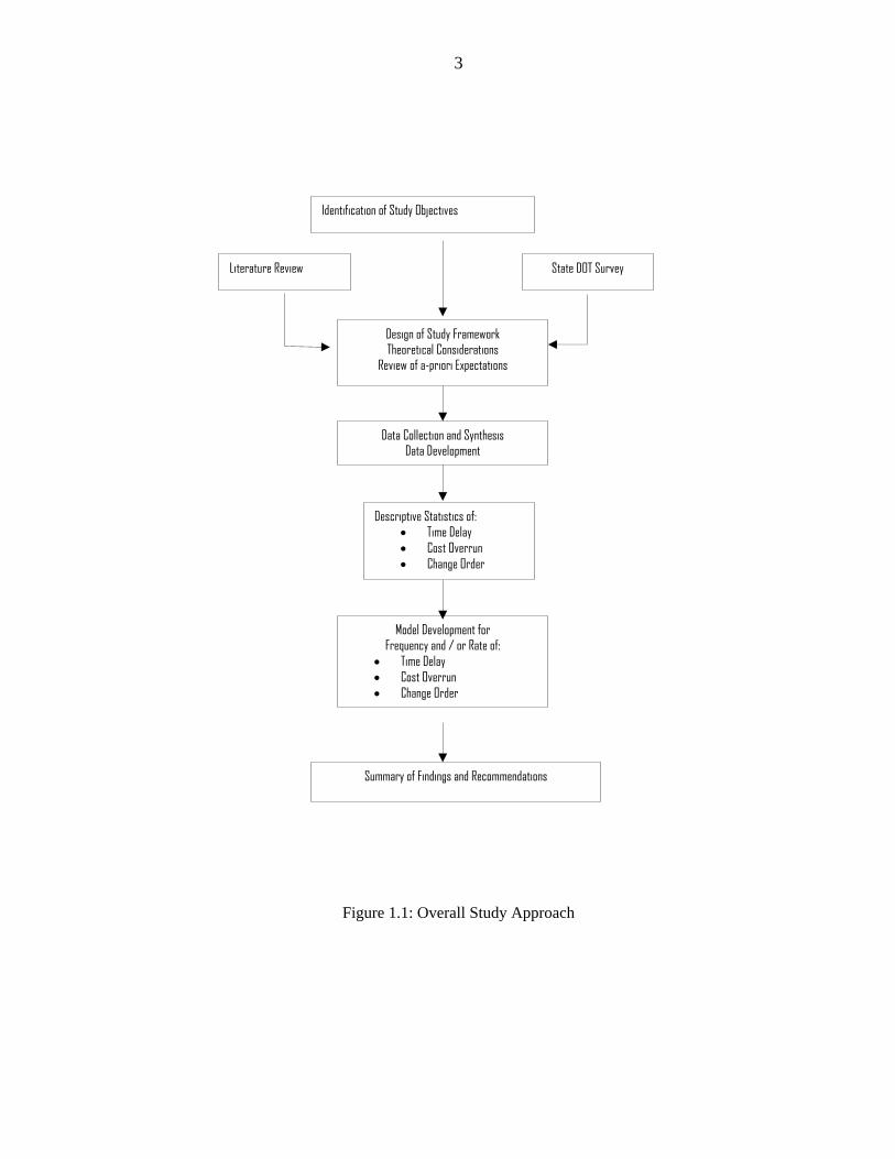
1.4 Overview of Study Approach
The overall approach of the study followed the steps shown in Figure 1.1. After establishing
the objectives, the study carries out a literature review and agency survey, and follows a study
framework that includes data collection and analysis. The data analysis is carried out using an array of
statistical methods that include descriptive statistics, correlation analysis, analysis of variance, pair-
wise tests, and statistical modeling. The study concludes with a set of recommendations for reducing
the problem of cost overruns, time delay and change orders associated with INDOT construction
projects.
3
Figure 1.1: Overall Study Approach
Design of Study Framework Theoretical Considerations
Review of a-priori Expectations
Data Collection and Synthesis Data Development
Identification of Study Objectives
Literature Review
State DOT Survey
Descriptive Statistics of: • Time Delay • Cost Overrun • Change Order
Model Development for Frequency and / or Rate of:
• Time Delay • Cost Overrun • Change Order
Summary of Findings and Recommendations
4
1.5 Organization of this Report
Chapter 1 of this report provides a general overview of the situation in Indiana concerning cost
overruns and time delays for INDOT projects. This section also highlights the objectives and scope of
the present study and provides a brief overview of the approach used in realizing the study objectives.
The literature review in Chapter 2 presents and discusses past findings and experience of previous
researchers in the areas related to the present study, such as change orders and root causes for time
delays. Chapter 3, which complements Chapter 2, presents and discusses the results of a survey of
state DOTs and provides a review of their contract management performances in terms of management
of cost overruns and time delays. Chapter 4 presents a framework for the analyses, discusses the
various methodologies used, and provides a theoretical basis to concepts used in the analysis for the
present study. In Chapter 5, the details of data collection are briefly described, as well as how the raw
data was processed and organized into a dataset using a format appropriate for the present (and
possible future) analysis of cost overruns and time delays in Indiana. Chapter 6 gives a preliminary
overview of the extent of the cost overruns and time delays problem in Indiana, using descriptive
statistics. Chapter 7 provides a preliminary statistical analysis of the dataset with, for example, the
analysis of variance and other statistical tools that enable an investigation of the trends that will appear
in the models. Chapter 8 presents the final results of the modeling process for cost overruns, time
delays, and change order prediction. Chapter 9 concludes the study with a summary of the findings.
This chapter also discusses the challenges faced during the study, implementation issues, and areas for
future investigation. In Chapter 10, recommendations are made for the reduction in the number of cost
overruns and time delays and to improve efficiency of project management and contract
administration. Implementation issues are discussed in Chapter 11.
5
CHAPTER 2: LITERATURE REVIEW
2.1 Introduction
This chapter identifies previous literature on the subject of cost overruns and time delays, and
provides a brief discussion of past findings. Also, the chapter reviews “standard taxonomy” that has
been used in this area. The reasons for cost overruns, time delays, and change orders as found in
previous studies are discussed, and examples of audit reports that analyze the problem of cost overruns
in past studies are provided.
2.2 Standard Taxonomy
Delay occurs when the progress of a contract falls behind its scheduled program. It may be
caused by any party to the contract and may be a direct result of one or more circumstances. A
contract delay has adverse effects on both the owner and contractor (either in the form of lost revenues
or extra expenses), often raises the contentious issue of delay responsibility, and may result in
conflicts that frequently reach the courts.
With regard to remedial measures, there are three types of delay (Rowland, 1981):
Excusable delay: the contractor is given a time extension but no additional money.
Concurrent delay: neither party recovers any damages.
Compensable delay: the contractor recovers monetary damages.
Majid and McCaffer [1998] provided similar categories of delay, on the basis of identified responsible
parties:
Compensable delays: responsibility borne by the client.
Non-excusable delays: responsibility borne by the contractor.
Excusable party delays: acts of God or a third party.
Cost overruns in construction contracts involve change orders and claims. Defining a “claim”
as the proposed changes to the contract that are being negotiated or litigated, Jahren and Ashe [1990]
identified two kinds of rates:
• The cost overrun rate, which is the percent difference in cost, (positive or negative) between
the final contract cost and the contract award amount,
6
• The change order rate, which is the ratio between the dollar amount of change orders and the
award amount.
The “final amount” was defined as the cost of the contract including change orders, and
outstanding claims and the dollar award amount is the dollar value at which the contract was awarded.
Change orders are “an indication that something on a construction project has not gone as
planned” (Rowland, 1981), and are associated with contract alterations such as additions, deletions, or
modifications to the contract. The consequences of change orders are additional cost, additional time
or both. Contract change orders can be requested by the owner, the contractor or third parties such as
local governments (O’Brien, 1998). Change orders are described as “unilateral” when signed only by
the contractor, owner or the party authorized by the changes clause in the conditions of the contract.
Change orders are referred to as “bilateral” when it is a mutual agreement or supplemental agreement.
The price of a change order can be expressed as a lump sum, a unit price, or the cost plus a fee, which
needs to be documented, estimated in terms of price and delay, and approved by both parties. A
change order is just as legally binding as the original construction contract. Few construction projects
are built without changes being made by the owner or by being necessary due to some unforeseen
circumstance (Rowland, 1981). Therefore, it may not be possible for any transportation agency to
completely eliminate change orders. Rather, efforts should be made to reduce their occurrence.
According to contract law, parties to a contract may modify the contract at any time by mutual
agreement. The owner’s right to order changes is offset by the contractor’s right to an equitable
adjustment in the contract price and time, to cover the cost of the work as changed. A change order can
imply extra or additional work, which are essentially two different concepts: extra work may not be
necessary for project completion and can be independent of the contract. Additional work may be
necessary because of errors or a change of plans and specifications.
Generally, the primary reasons for actual costs varying from a contractor’s original bid price
are changes in the scope of the work to be done and incorrect estimates of the work quantities included
in the original bid specifications. Contractor errors include unnecessary work, work that is not
according to design plans, and work or materials that do not meet contract specifications. On the other
hand, contracting agency errors include planning and design deficiencies such as revisions in the scope
of the work, added work, and revisions in quantities in the project design. Unforeseen circumstances
include site conditions that differ from those described in the contract documents.
7
2.3 Causes of Time Delays
Non-excusable delays are generally the responsibility of the contractor, and the agency may be
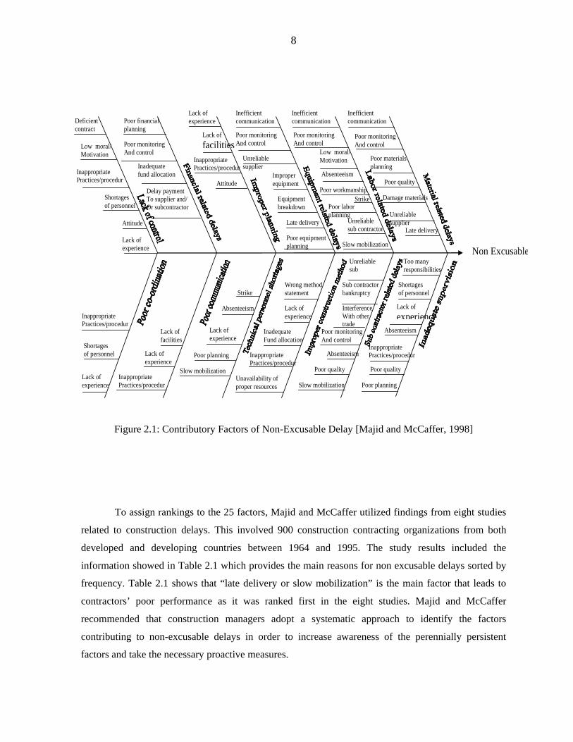
entitled to claim damages. In studying non-excusable delays, Majid and McCaffer [1998] discussed
methods to document the factors of non-excusable delays using a fishbone diagram and ranking
methodology, the steps for which are explained below. The fish bone diagram, shown in Figure 1,
enables the identification of contract problems at a micro level and consequently helps to search for
the root causes. Majid and McCaffer defined 12 main causes:
1. Materials-related delays
2. Labor-related delays
3. Equipment-related delays
4. Financial delays
5. Improper planning
6. Lack of control
7. Subcontractor delays
8. Poor coordination
9. Inadequate supervision
10. Improper construction methods
11. Technical personnel shortages
12. Poor communication
Materials-related delays include late delivery, damage, or poor quality of materials. Labor-
related delays can be due to low motivation, poor communication or absenteeism. Equipment-related
delays can be due to poor equipment planning. Improper planning can be due to a lack of experience.
Financial-related delays concern financial planning or delayed payment to suppliers. Lack of control,
poor coordination, technical personnel shortage and poor communication are representative of poor
management of personnel and the whole agency. Improper construction method is related to items
such as a wrong method statement. Subcontractor-related delays include not only items that are the
fault of the subcontractor but also of the agency’s employees because of absenteeism or slow
mobilization. The problem of inadequate supervision concerns managers who, for instance, have too
many responsibilities or few management skills. Each main cause of non-excusable delays comprises
several contributing factors. Some factors, such as poor monitoring and control, poor planning, and
lack of experience, are common to more than one main cause. A total of 25 factors were identified by
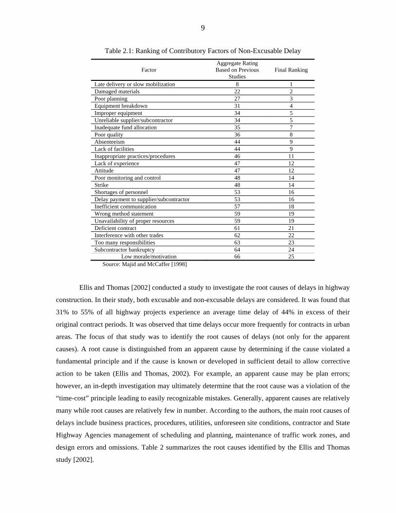
Majid and McCaffer [1998] as shown in Table 2.1.
8
Figure 2.1: Contributory Factors of Non-Excusable Delay [Majid and McCaffer, 1998]
To assign rankings to the 25 factors, Majid and McCaffer utilized findings from eight studies
related to construction delays. This involved 900 construction contracting organizations from both
developed and developing countries between 1964 and 1995. The study results included the
information showed in Table 2.1 which provides the main reasons for non excusable delays sorted by
frequency. Table 2.1 shows that “late delivery or slow mobilization” is the main factor that leads to
contractors’ poor performance as it was ranked first in the eight studies. Majid and McCaffer
recommended that construction managers adopt a systematic approach to identify the factors
contributing to non-excusable delays in order to increase awareness of the perennially persistent
factors and take the necessary proactive measures.
Inappropriate Practices/procedur
Lack of experience
Attitude
Shortages of personnel
Non Excusable
Deficient contract
Low moral/ Motivation
Poor financial planning
Poor monitoring And control
Inadequate fund allocation
Delay payment To supplier and/ Or subcontractor
Lack of experience
Lack of facilities
Inappropriate Practices/procedur
Attitude
Inefficient communication
Inefficient communication
Inefficient communication
Lack of experience
Lack of experience
Lack of experience
Lack of experience
Poor monitoring And control
Poor monitoring And control
Poor monitoring And control
Poor monitoring And control
Unreliable supplier
Improper equipment
Equipment breakdown
Late delivery
Poor equipment planning
Low moral/ Motivation
Absenteeism
Strike
Strike
Absenteeism
Absenteeism
Absenteeism
Lack of experience
Poor materials planning
Poor quality
Poor quality
Poor planning
Inappropriate Practices/procedur
Poor quality
Inappropriate Practices/procedur
Poor workmanship
Poor labor planning
Unreliable sub contractor
Slow mobilization
Unreliable supplier
Damage materials
Late delivery
Inappropriate Practices/procedur
Lack of facilities
Shortages of personnel
Inappropriate Practices/procedur
Poor planning
Slow mobilization
Wrong method statement
Inadequate Fund allocation
Unavailability of proper resources
Unreliable sub
Interference With other trade
Slow mobilization
Shortages of personnel
Too many responsibilities
Sub contractor bankruptcy
9
Table 2.1: Ranking of Contributory Factors of Non-Excusable Delay
Factor Aggregate Rating Based on Previous
Studies Final Ranking
Late delivery or slow mobilization 8 1 Damaged materials 22 2 Poor planning 27 3 Equipment breakdown 31 4 Improper equipment 34 5 Unreliable supplier/subcontractor 34 5 Inadequate fund allocation 35 7 Poor quality 36 8 Absenteeism 44 9 Lack of facilities 44 9 Inappropriate practices/procedures 46 11 Lack of experience 47 12 Attitude 47 12 Poor monitoring and control 48 14 Strike 48 14 Shortages of personnel 53 16 Delay payment to supplier/subcontractor 53 16 Inefficient communication 57 18 Wrong method statement 59 19 Unavailability of proper resources 59 19 Deficient contract 61 21 Interference with other trades 62 22 Too many responsibilities 63 23 Subcontractor bankruptcy 64 24
Low morale/motivation 66 25 Source: Majid and McCaffer [1998]
Ellis and Thomas [2002] conducted a study to investigate the root causes of delays in highway
construction. In their study, both excusable and non-excusable delays are considered. It was found that
31% to 55% of all highway projects experience an average time delay of 44% in excess of their
original contract periods. It was observed that time delays occur more frequently for contracts in urban
areas. The focus of that study was to identify the root causes of delays (not only for the apparent
causes). A root cause is distinguished from an apparent cause by determining if the cause violated a
fundamental principle and if the cause is known or developed in sufficient detail to allow corrective
action to be taken (Ellis and Thomas, 2002). For example, an apparent cause may be plan errors;
however, an in-depth investigation may ultimately determine that the root cause was a violation of the
“time-cost” principle leading to easily recognizable mistakes. Generally, apparent causes are relatively
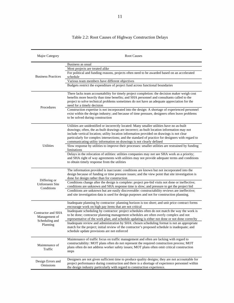
many while root causes are relatively few in number. According to the authors, the main root causes of
delays include business practices, procedures, utilities, unforeseen site conditions, contractor and State
Highway Agencies management of scheduling and planning, maintenance of traffic work zones, and
design errors and omissions. Table 2 summarizes the root causes identified by the Ellis and Thomas
study [2002].
10
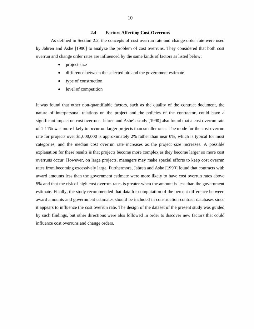
2.4 Factors Affecting Cost-Overruns
As defined in Section 2.2, the concepts of cost overrun rate and change order rate were used
by Jahren and Ashe [1990] to analyze the problem of cost overruns. They considered that both cost
overrun and change order rates are influenced by the same kinds of factors as listed below:
• project size
• difference between the selected bid and the government estimate
• type of construction
• level of competition
It was found that other non-quantifiable factors, such as the quality of the contract document, the
nature of interpersonal relations on the project and the policies of the contractor, could have a
significant impact on cost overruns. Jahren and Ashe’s study [1990] also found that a cost overrun rate
of 1-11% was more likely to occur on larger projects than smaller ones. The mode for the cost overrun
rate for projects over $1,000,000 is approximately 2% rather than near 0%, which is typical for most
categories, and the median cost overrun rate increases as the project size increases. A possible
explanation for these results is that projects become more complex as they become larger so more cost
overruns occur. However, on large projects, managers may make special efforts to keep cost overrun
rates from becoming excessively large. Furthermore, Jahren and Ashe [1990] found that contracts with
award amounts less than the government estimate were more likely to have cost overrun rates above
5% and that the risk of high cost overrun rates is greater when the amount is less than the government
estimate. Finally, the study recommended that data for computation of the percent difference between
award amounts and government estimates should be included in construction contract databases since
it appears to influence the cost overrun rate. The design of the dataset of the present study was guided
by such findings, but other directions were also followed in order to discover new factors that could
influence cost overruns and change orders.
11
Table 2.2: Root Causes of Highway Construction Delays
Major Category
Root Causes
Business as usual Most projects are treated alike For political and funding reasons, projects often need to be awarded based on an accelerated schedule Various team members have different objectives
Business Practices
Budgets restrict the expenditure of project fund across functional boundaries There lacks team accountability for timely project completion: the decision maker weigh cost benefits more heavily than time benefits; and SHA personnel and consultants called to the project to solve technical problems sometimes do not have an adequate appreciation for the need for a timely decision Procedures Construction expertise is not incorporated into the design: A shortage of experienced personnel exist within the design industry; and because of time pressure, designers often leave problems to be solved during construction Utilities are unidentified or incorrectly located: Many smaller utilities have no as-built drawings; often, the as-built drawings are incorrect; as-built location information may not include vertical location; utility location information provided on drawings is not clear particularly for complex intersections; and the standard of practice for designers with regard to communicating utility information on drawings is not clearly defined Slow response by utilities to improve their processes: smaller utilities are restrained by funding limitations
Utilities
Delays in the relocation of utilities: utilities companies may not see SHA work as a priority; and SHA right of way agreements with utilities may not provide adequate terms and conditions to obtain timely response from the utilities The information provided is inaccurate: conditions are known but not incorporated into the design because of funding or time pressure issues; and the view point that site investigation is done for design rather than for construction Conditions change after the design is complete: project pre-bid visits not done or ineffective; conditions are unknown and SHA response time is slow; and pressure to get the project bid
Differing or Unforeseen Site
Conditions Conditions are unknown but are easily discoverable: constructability reviews are ineffective; and site investigation data is used for design purposes and not for construction planning. Inadequate planning by contractor: planning horizon is too short; and unit price contract forms encourage work on high pay items that are not critical Inadequate scheduling by contractor: project schedules often do not match the way the work is to be done; contractor planning management schedules are often overly complex and not representative of the work plan; and schedule updating is either not done or not done correclty
Contractor and SHA Management of Scheduling and
Planning Inadequate review and administration by SHA: chosen scheduling format is not an appropriate match for the project; initial review of the contractor’s proposed schedule is inadequate; and schedule update provisions are not enforced
Maintenance of Traffic
Maintenance of traffic focus on traffic management and often are lacking with regard to constructability: MOT plans often do not represent the required construction process; MOT plans often do not address worker safety issues; MOT plans often omit critical construction steps
Design Errors and Omissions
Designers are not given sufficient time to produce quality designs; they are not accountable for project performance during construction and there is a shortage of experience personnel within the design industry particularly with regard to construction experience.
12
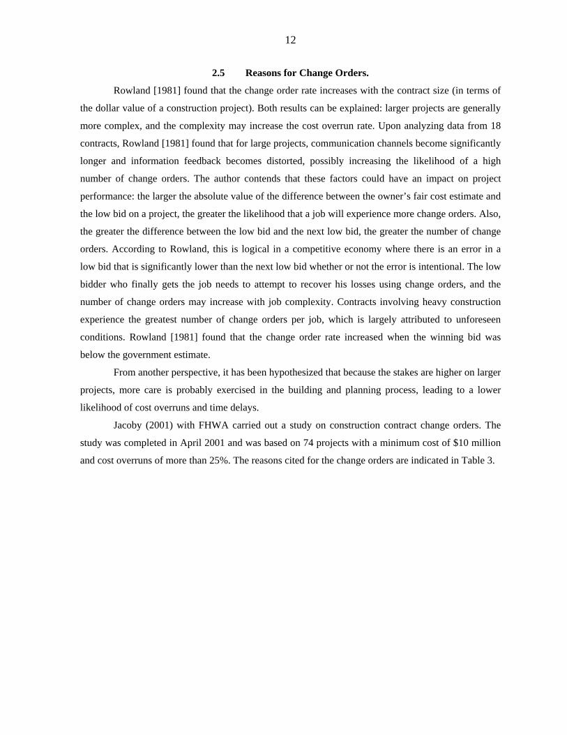
2.5 Reasons for Change Orders.
Rowland [1981] found that the change order rate increases with the contract size (in terms of
the dollar value of a construction project). Both results can be explained: larger projects are generally
more complex, and the complexity may increase the cost overrun rate. Upon analyzing data from 18
contracts, Rowland [1981] found that for large projects, communication channels become significantly
longer and information feedback becomes distorted, possibly increasing the likelihood of a high
number of change orders. The author contends that these factors could have an impact on project
performance: the larger the absolute value of the difference between the owner’s fair cost estimate and
the low bid on a project, the greater the likelihood that a job will experience more change orders. Also,
the greater the difference between the low bid and the next low bid, the greater the number of change
orders. According to Rowland, this is logical in a competitive economy where there is an error in a
low bid that is significantly lower than the next low bid whether or not the error is intentional. The low
bidder who finally gets the job needs to attempt to recover his losses using change orders, and the
number of change orders may increase with job complexity. Contracts involving heavy construction
experience the greatest number of change orders per job, which is largely attributed to unforeseen
conditions. Rowland [1981] found that the change order rate increased when the winning bid was
below the government estimate.
From another perspective, it has been hypothesized that because the stakes are higher on larger
projects, more care is probably exercised in the building and planning process, leading to a lower
likelihood of cost overruns and time delays.
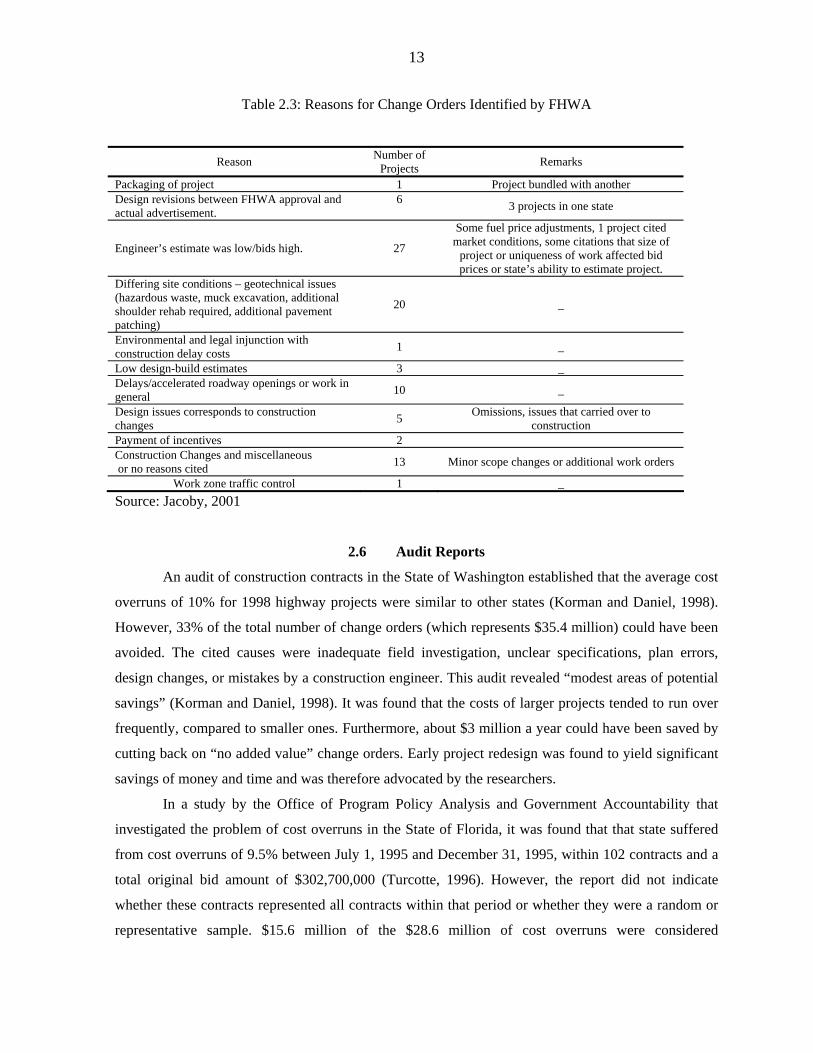
Jacoby (2001) with FHWA carried out a study on construction contract change orders. The
study was completed in April 2001 and was based on 74 projects with a minimum cost of $10 million
and cost overruns of more than 25%. The reasons cited for the change orders are indicated in Table 3.
13
Table 2.3: Reasons for Change Orders Identified by FHWA
Reason Number of Projects Remarks
Packaging of project 1 Project bundled with another Design revisions between FHWA approval and actual advertisement.
6 3 projects in one state
Engineer’s estimate was low/bids high. 27
Some fuel price adjustments, 1 project cited market conditions, some citations that size of
project or uniqueness of work affected bid prices or state’s ability to estimate project.
Differing site conditions – geotechnical issues (hazardous waste, muck excavation, additional shoulder rehab required, additional pavement patching)
20 _
Environmental and legal injunction with construction delay costs 1 _
Low design-build estimates 3 _ Delays/accelerated roadway openings or work in general 10 _
Design issues corresponds to construction changes 5 Omissions, issues that carried over to
construction Payment of incentives 2 Construction Changes and miscellaneous or no reasons cited 13 Minor scope changes or additional work orders
Work zone traffic control 1 _ Source: Jacoby, 2001
2.6 Audit Reports
An audit of construction contracts in the State of Washington established that the average cost
overruns of 10% for 1998 highway projects were similar to other states (Korman and Daniel, 1998).
However, 33% of the total number of change orders (which represents $35.4 million) could have been
avoided. The cited causes were inadequate field investigation, unclear specifications, plan errors,
design changes, or mistakes by a construction engineer. This audit revealed “modest areas of potential
savings” (Korman and Daniel, 1998). It was found that the costs of larger projects tended to run over
frequently, compared to smaller ones. Furthermore, about $3 million a year could have been saved by
cutting back on “no added value” change orders. Early project redesign was found to yield significant
savings of money and time and was therefore advocated by the researchers.
In a study by the Office of Program Policy Analysis and Government Accountability that
investigated the problem of cost overruns in the State of Florida, it was found that that state suffered
from cost overruns of 9.5% between July 1, 1995 and December 31, 1995, within 102 contracts and a
total original bid amount of $302,700,000 (Turcotte, 1996). However, the report did not indicate
whether these contracts represented all contracts within that period or whether they were a random or
representative sample. $15.6 million of the $28.6 million of cost overruns were considered
14
“avoidable” costs. Furthermore, approximately $4.2 million of the avoidable costs were considered
wasted money because they did not add value for citizens. The Florida study sought to identify the
responsibility for such “wasted money,” which was supposedly shared among consultants (32%), third
parties (utility companies, permitting agencies, and local governments (55%), and the highway agency
staff (13%). The report stated that cost overruns are perceived as being avoidable when they occur due
to design plan or project management problems that were reasonably foreseeable and preventable. The
reported further asserted that cost overruns may add value to projects by producing a better product,
but duly noted that in many cases, cost overruns do not add value and are therefore considered as
“wasted money.” It was found that consultants and third parties in the Florida study were responsible
for more avoidable cost overruns (38% for both) than agency staff (24%), but the part of cost overruns
that do not add value to the project was less for consultants than for agency staff. Finally, in a bid to
minimize cost overruns from occurring and to hold responsible parties accountable, Turcotte (1996)
made the following recommendations for the Office for Program Policy Analysis and Government
Accountability:
• Develop statewide criteria to assess the effectiveness of pursuing recovery of cost overruns
that are attributable to consultants that do not add value to projects.
• Develop criteria for including avoidable cost overruns that do not add value in the selection
process for awarding future contracts to consultants.
• Develop criteria for including avoidable cost overruns that do not add value in determining the
constructability grades for design work.
• Provide an interim constructability grade during the construction process in addition to a final
grade.
• Monitor responses to the monthly report of consultant performance grades.
• Modify DOT personnel policies and procedures to include evaluating DOT design staff for the
impact of avoidable cost overruns that do not add value.
• Continue implementing strategies to improve the quality of construction plans to resolve plan
problems prior to letting contracts for bid and monitor progress toward reducing cost overruns.
• Continue improving coordination with third parties to incorporate design changes and to
identify utility lines as plans are developed to minimize cost overruns due to delays in making
design changes during construction.
In Delaware (Wagner, 1998), the state DOT (DelDOT) experienced 13.9% cost overruns
between 1994 and 1996 with a total bid amount of $114,200,000 for 148 contracts. From an economic
and efficiency audit study commissioned by the state, Wagner [1998] found that the main causes were
15
changes in the work scope and incorrect estimates of the work quantities in the original bid
specifications. According to the author, these reasons are probably due to contractor error
(unnecessary work, design plans, poor contract specifications), contracting agency error (planning and
design deficiencies: scope of work, added work, and revisions in quantities) and unforeseen
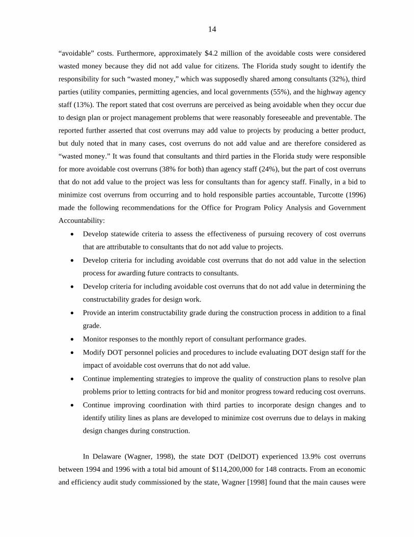
circumstances (archeological discovery). The report for that study concluded with a set of
recommendations (Table 4) covering issues such as considering alternative options for higher cost-
effectiveness, developing bid a analysis system and a tracking system for project payment revisions,
evaluating contractors, developing other performance measures, and updating the procedure manuals.
Table 2.4: Recommendations for Addressing Cost Overruns at DelDOT [Wagner, 1998].
Number
Recommendations
1
Evaluation of the need for alternative contracting options to ensure that statutory and other regulatory restrictions do not significantly impact the efficient use of taxpayers funds. For example, DelDOT could consider a policy that would allow re-negotiation of unit prices in certain instances even though the threshold for a Supplement Agreement is not reached.
2 Completion of the development of the bid analysis system.
3 Completion of all aspects of the Project Payment Tracking System so that management has comprehensive, reliable information regarding change orders.
4 Revision of contracts to allow the State to recover additional costs incurred as a result of errors and omissions of consultants.
5 Continued establishment procedures that will ensure more accurate contract design quantities which will provide better engineer estimates of costs before the project goes out to bid.
6 Continued formal tracking both preliminary design requests and input from plan reviewers. The plan reviewers should be held accountable for non-compliance review deadlines.
7 Continued implementation of a formal budgetary control process which ensures that each change order is afforded an appropriate level of management review.
8
Review of post construction contract review process to insure that its stated objective of decreasing plan revisions, change orders, and construction claims is attained and resulting improvements to contract economy and efficiency are documented.
9 Completion of contractor evaluations and use as part of the pre-award evaluation process.
10 Implementation of a plan to ensure that highway construction contracts are afforded sufficient audit coverage.
11 Development of additional performance measures to provide management with more comprehensive data to assess performance.
12 Ensuring that DelDOT processes provide for appropriate reporting of performance measurement, such as, consistent reporting periods.
13 Update of DelDOT’s Highway Construction Manual and the Contract Administration Procedures Manual.
16
In response to the above recommendations, DelDOT indicated agreement with only some of
them, adding that some were already being implemented and needed time for their effectiveness to be
manifest. For instance, Recommendation #7 would be addressed with Recommendation #3 by
completing the Project Payment Tracking System. Regarding Recommendation #9, DelDOT stated
that a decision had been made several years ago to carry out contractor evaluation. In
Recommendation #11 DelDOT considered that there was no “correct” number of performance
measures and the fact that other states used more performance measures did not mean that the
DelDOT system was deficient. Finally, for Recommendation #13 DelDOT agreed with the need for
regular updating of performance measures.
2.6 Discussion of the Literature Review
2.7
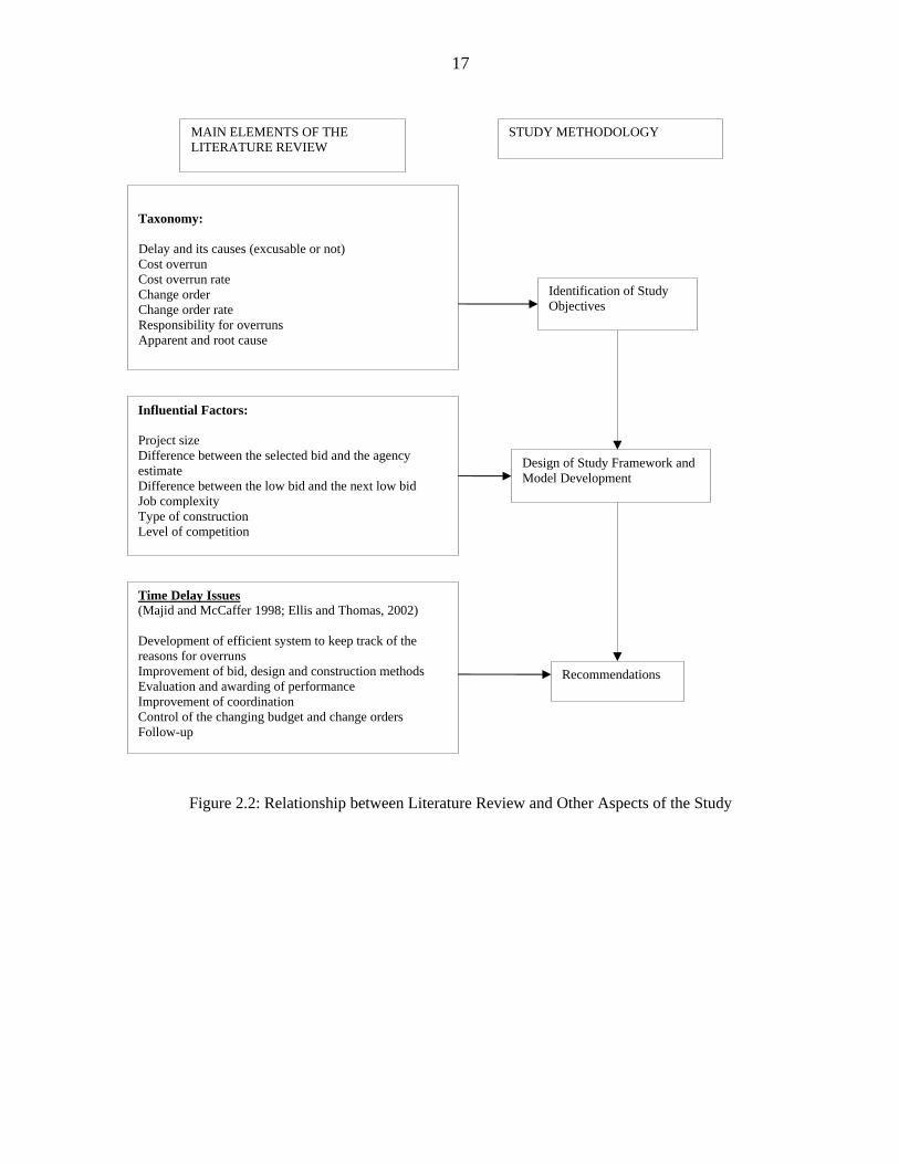
Figure 2.2 summarizes the main elements of the literature review and indicates how the
findings of the review relate to the framework of the present study. First, the literature review enabled
definition of key terms for the present study. Rowland’s study [1981], for example, provided some
terms and identified some influential factors affecting change orders. The discussions in Sections 2.3,
2.4, and 2.5 are the basis for comparing the results of the present study to the previous ones. The
information in the present chapter provides an indication of issues faced by transportation agencies in
managing cost overruns and time delays. While preparing the recommendations for INDOT, it may be
helpful to make the distinction between root causes and apparent causes as defined in the Ellis and
Thomas’ study [2002].
2.8 Chapter Summary
The literature review identified the problems of cost overruns and time delay with some new
and external points of view and provided definitions of the key concepts. Previous studies identified
some factors that influence cost overruns or time delays and developed tools that help address such
problems.
17
Figure 2.2: Relationship between Literature Review and Other Aspects of the Study
MAIN ELEMENTS OF THE LITERATURE REVIEW
STUDY METHODOLOGY
Taxonomy: Delay and its causes (excusable or not) Cost overrun Cost overrun rate Change order Change order rate Responsibility for overruns Apparent and root cause
Identification of Study Objectives
Influential Factors: Project size Difference between the selected bid and the agency estimate Difference between the low bid and the next low bid Job complexity Type of construction Level of competition
Design of Study Framework and Model Development
Recommendations
Time Delay Issues (Majid and McCaffer 1998; Ellis and Thomas, 2002) Development of efficient system to keep track of the reasons for overruns Improvement of bid, design and construction methods Evaluation and awarding of performance Improvement of coordination Control of the changing budget and change orders Follow-up
18
CHAPTER 3: AGENCY SURVEY
3.1 Introduction
An agency survey was carried out to complement the findings from the literature review and
to acquire current state of practice perspectives on the problem of cost overruns, time delay and
change orders. The agency survey was also motivated by the success of a fairly recent similar effort by
Jacoby (2001) who conducted an AASHTO-FHWA sponsored nationwide survey to ask DOTs about
the various methods they use to manage cost overruns and time delays through their change order
classifications. The experience of other states would therefore be helpful in establishing appropriate
recommendations for INDOT. Two aspects of overruns were compared: the frequency and amount of
cost overruns and time delays, and how such problems are addressed. An email solicitation (Appendix
B) was distributed through the Research Division of INDOT and posted on a national DOT research
list requesting information on cost overruns and time delays. This solicitation yielded 11 responses
from other state DOTs in the form of either direct responses to email questions or provision of
attached electronic documents. This chapter presents and discusses the responses to the agency survey
conducted as part of the present study. The cost overrun amounts herein presented constitute an
average of several contracts in any single year and therefore may not reveal variations of cost overruns
and underruns across individual contracts. In subsequent chapters, both cost underruns and overruns,
rather than their combined average, are presented separately using Indiana data.
3.2 Cost Overruns and Time Delays: Results of the Agency Survey
Eleven state transportation agencies responded to the e-mail request: Arkansas, Idaho, Illinois,
Iowa, Maryland, Missouri, New Mexico, Ohio, Oregon, Tennessee, and Texas. The respondent from
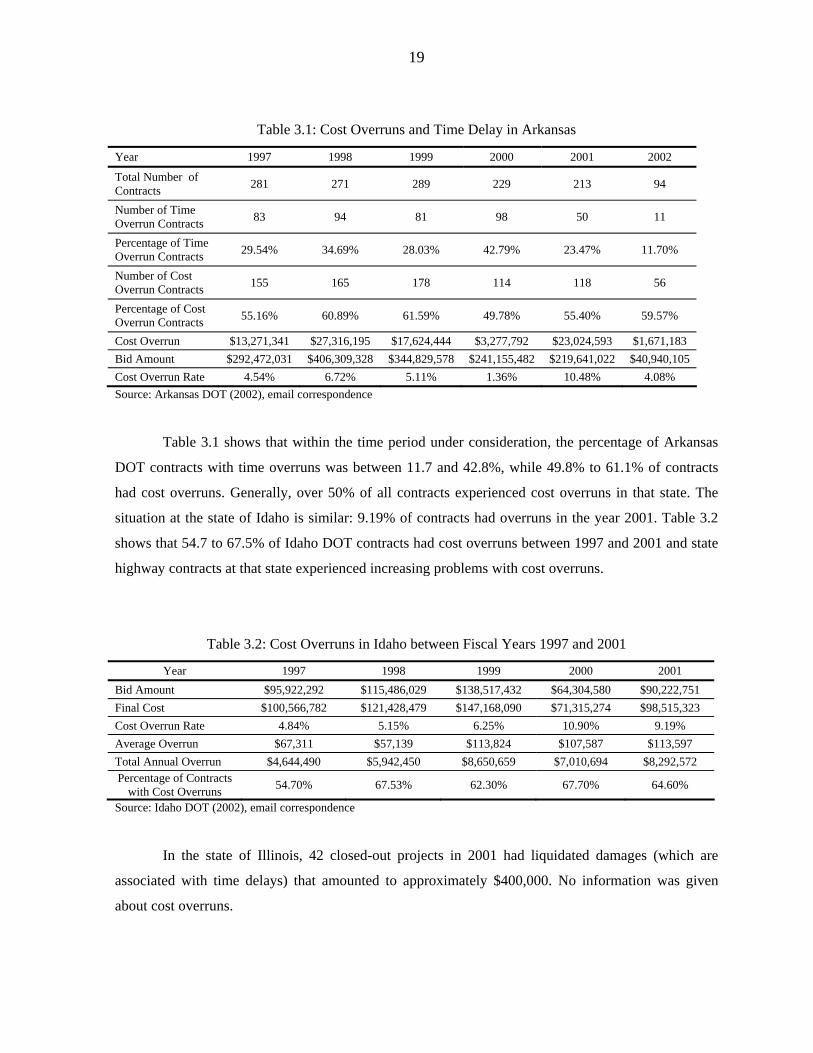
Arkansas indicated that his state is increasingly experiencing cost overruns, with a record cost overrun
rate of over 10% occurring in 2001. Table 3.1 shows the trends in cost overruns and time delays for
Arkansas DOT projects from 1997 to 2002.
19
Table 3.1: Cost Overruns and Time Delay in Arkansas
Year 1997 1998 1999 2000 2001 2002
Total Number of Contracts 281 271 289 229 213 94
Number of Time Overrun Contracts 83 94 81 98 50 11
Percentage of Time Overrun Contracts 29.54% 34.69% 28.03% 42.79% 23.47% 11.70%
Number of Cost Overrun Contracts 155 165 178 114 118 56
Percentage of Cost Overrun Contracts 55.16% 60.89% 61.59% 49.78% 55.40% 59.57%
Cost Overrun $13,271,341 $27,316,195 $17,624,444 $3,277,792 $23,024,593 $1,671,183 Bid Amount $292,472,031 $406,309,328 $344,829,578 $241,155,482 $219,641,022 $40,940,105 Cost Overrun Rate 4.54% 6.72% 5.11% 1.36% 10.48% 4.08% Source: Arkansas DOT (2002), email correspondence
Table 3.1 shows that within the time period under consideration, the percentage of Arkansas
DOT contracts with time overruns was between 11.7 and 42.8%, while 49.8% to 61.1% of contracts
had cost overruns. Generally, over 50% of all contracts experienced cost overruns in that state. The
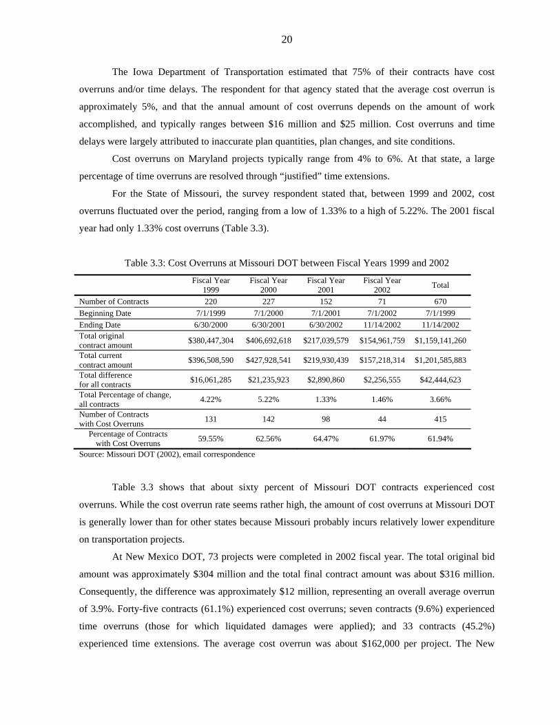
situation at the state of Idaho is similar: 9.19% of contracts had overruns in the year 2001. Table 3.2
shows that 54.7 to 67.5% of Idaho DOT contracts had cost overruns between 1997 and 2001 and state
highway contracts at that state experienced increasing problems with cost overruns.
Table 3.2: Cost Overruns in Idaho between Fiscal Years 1997 and 2001
Year 1997 1998 1999 2000 2001 Bid Amount $95,922,292 $115,486,029 $138,517,432 $64,304,580 $90,222,751 Final Cost $100,566,782 $121,428,479 $147,168,090 $71,315,274 $98,515,323 Cost Overrun Rate 4.84% 5.15% 6.25% 10.90% 9.19% Average Overrun $67,311 $57,139 $113,824 $107,587 $113,597 Total Annual Overrun $4,644,490 $5,942,450 $8,650,659 $7,010,694 $8,292,572 Percentage of Contracts
with Cost Overruns 54.70% 67.53% 62.30% 67.70% 64.60%
Source: Idaho DOT (2002), email correspondence
In the state of Illinois, 42 closed-out projects in 2001 had liquidated damages (which are
associated with time delays) that amounted to approximately $400,000. No information was given
about cost overruns.
20
The Iowa Department of Transportation estimated that 75% of their contracts have cost
overruns and/or time delays. The respondent for that agency stated that the average cost overrun is
approximately 5%, and that the annual amount of cost overruns depends on the amount of work
accomplished, and typically ranges between $16 million and $25 million. Cost overruns and time
delays were largely attributed to inaccurate plan quantities, plan changes, and site conditions.
Cost overruns on Maryland projects typically range from 4% to 6%. At that state, a large
percentage of time overruns are resolved through “justified” time extensions.
For the State of Missouri, the survey respondent stated that, between 1999 and 2002, cost
overruns fluctuated over the period, ranging from a low of 1.33% to a high of 5.22%. The 2001 fiscal
year had only 1.33% cost overruns (Table 3.3).
Table 3.3: Cost Overruns at Missouri DOT between Fiscal Years 1999 and 2002
Fiscal Year 1999
Fiscal Year 2000
Fiscal Year 2001
Fiscal Year 2002 Total
Number of Contracts 220 227 152 71 670 Beginning Date 7/1/1999 7/1/2000 7/1/2001 7/1/2002 7/1/1999 Ending Date 6/30/2000 6/30/2001 6/30/2002 11/14/2002 11/14/2002 Total original contract amount $380,447,304 $406,692,618 $217,039,579 $154,961,759 $1,159,141,260
Total current contract amount $396,508,590 $427,928,541 $219,930,439 $157,218,314 $1,201,585,883
Total difference for all contracts $16,061,285 $21,235,923 $2,890,860 $2,256,555 $42,444,623
Total Percentage of change, all contracts 4.22% 5.22% 1.33% 1.46% 3.66%
Number of Contracts with Cost Overruns 131 142 98 44 415
Percentage of Contracts with Cost Overruns 59.55% 62.56% 64.47% 61.97% 61.94%
Source: Missouri DOT (2002), email correspondence
Table 3.3 shows that about sixty percent of Missouri DOT contracts experienced cost
overruns. While the cost overrun rate seems rather high, the amount of cost overruns at Missouri DOT
is generally lower than for other states because Missouri probably incurs relatively lower expenditure
on transportation projects.
At New Mexico DOT, 73 projects were completed in 2002 fiscal year. The total original bid
amount was approximately $304 million and the total final contract amount was about $316 million.
Consequently, the difference was approximately $12 million, representing an overall average overrun
of 3.9%. Forty-five contracts (61.1%) experienced cost overruns; seven contracts (9.6%) experienced
time overruns (those for which liquidated damages were applied); and 33 contracts (45.2%)
experienced time extensions. The average cost overrun was about $162,000 per project. The New
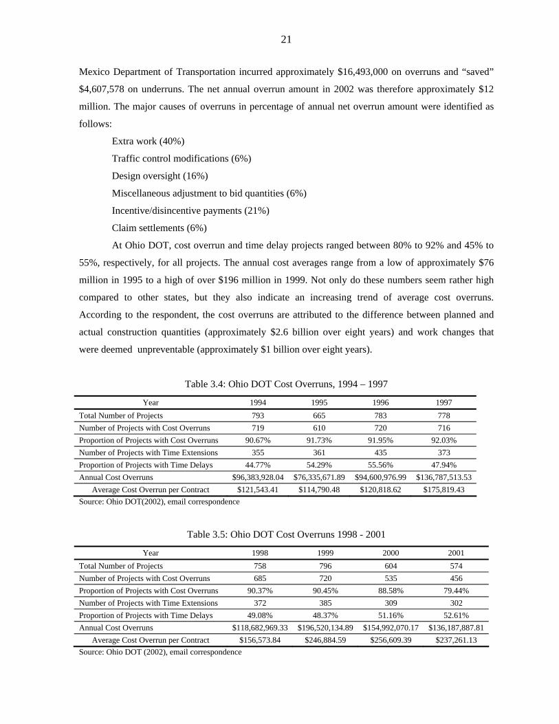
21
Mexico Department of Transportation incurred approximately $16,493,000 on overruns and “saved”
$4,607,578 on underruns. The net annual overrun amount in 2002 was therefore approximately $12
million. The major causes of overruns in percentage of annual net overrun amount were identified as
follows:
Extra work (40%)
Traffic control modifications (6%)
Design oversight (16%)
Miscellaneous adjustment to bid quantities (6%)
Incentive/disincentive payments (21%)
Claim settlements (6%)
At Ohio DOT, cost overrun and time delay projects ranged between 80% to 92% and 45% to
55%, respectively, for all projects. The annual cost averages range from a low of approximately $76
million in 1995 to a high of over $196 million in 1999. Not only do these numbers seem rather high
compared to other states, but they also indicate an increasing trend of average cost overruns.
According to the respondent, the cost overruns are attributed to the difference between planned and
actual construction quantities (approximately $2.6 billion over eight years) and work changes that
were deemed unpreventable (approximately $1 billion over eight years).
Table 3.4: Ohio DOT Cost Overruns, 1994 – 1997
Year 1994 1995 1996 1997 Total Number of Projects 793 665 783 778 Number of Projects with Cost Overruns 719 610 720 716 Proportion of Projects with Cost Overruns 90.67% 91.73% 91.95% 92.03% Number of Projects with Time Extensions 355 361 435 373 Proportion of Projects with Time Delays 44.77% 54.29% 55.56% 47.94% Annual Cost Overruns $96,383,928.04 $76,335,671.89 $94,600,976.99 $136,787,513.53
Average Cost Overrun per Contract $121,543.41 $114,790.48 $120,818.62 $175,819.43 Source: Ohio DOT(2002), email correspondence
Table 3.5: Ohio DOT Cost Overruns 1998 - 2001
Year 1998 1999 2000 2001 Total Number of Projects 758 796 604 574 Number of Projects with Cost Overruns 685 720 535 456 Proportion of Projects with Cost Overruns 90.37% 90.45% 88.58% 79.44% Number of Projects with Time Extensions 372 385 309 302 Proportion of Projects with Time Delays 49.08% 48.37% 51.16% 52.61% Annual Cost Overruns $118,682,969.33 $196,520,134.89 $154,992,070.17 $136,187,887.81
Average Cost Overrun per Contract $156,573.84 $246,884.59 $256,609.39 $237,261.13 Source: Ohio DOT (2002), email correspondence
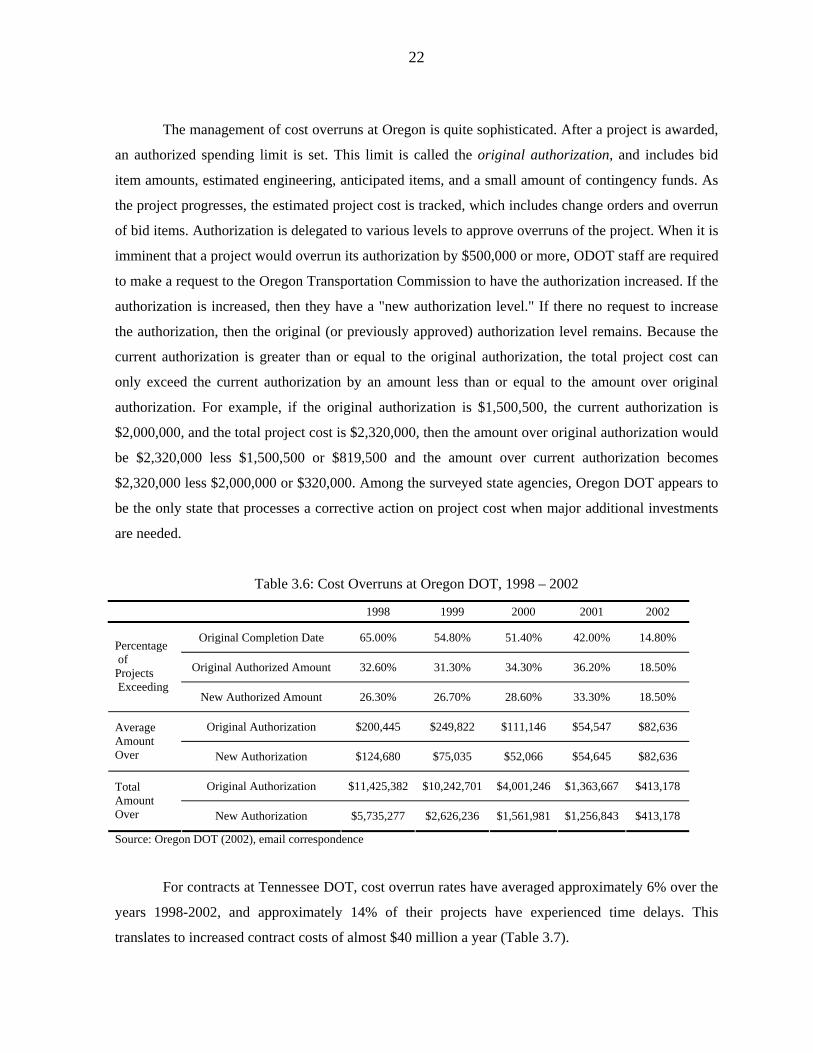
22
The management of cost overruns at Oregon is quite sophisticated. After a project is awarded,
an authorized spending limit is set. This limit is called the original authorization, and includes bid
item amounts, estimated engineering, anticipated items, and a small amount of contingency funds. As
the project progresses, the estimated project cost is tracked, which includes change orders and overrun
of bid items. Authorization is delegated to various levels to approve overruns of the project. When it is
imminent that a project would overrun its authorization by $500,000 or more, ODOT staff are required
to make a request to the Oregon Transportation Commission to have the authorization increased. If the
authorization is increased, then they have a "new authorization level." If there no request to increase
the authorization, then the original (or previously approved) authorization level remains. Because the
current authorization is greater than or equal to the original authorization, the total project cost can
only exceed the current authorization by an amount less than or equal to the amount over original
authorization. For example, if the original authorization is $1,500,500, the current authorization is
$2,000,000, and the total project cost is $2,320,000, then the amount over original authorization would
be $2,320,000 less $1,500,500 or $819,500 and the amount over current authorization becomes
$2,320,000 less $2,000,000 or $320,000. Among the surveyed state agencies, Oregon DOT appears to
be the only state that processes a corrective action on project cost when major additional investments
are needed.
Table 3.6: Cost Overruns at Oregon DOT, 1998 – 2002
1998 1999 2000 2001 2002
Original Completion Date 65.00% 54.80% 51.40% 42.00% 14.80%
Original Authorized Amount 32.60% 31.30% 34.30% 36.20% 18.50%
Percentage of Projects Exceeding
New Authorized Amount 26.30% 26.70% 28.60% 33.30% 18.50%
Original Authorization $200,445 $249,822 $111,146 $54,547 $82,636 Average Amount Over New Authorization $124,680 $75,035 $52,066 $54,645 $82,636
Original Authorization $11,425,382 $10,242,701 $4,001,246 $1,363,667 $413,178 Total Amount Over New Authorization $5,735,277 $2,626,236 $1,561,981 $1,256,843 $413,178
Source: Oregon DOT (2002), email correspondence
For contracts at Tennessee DOT, cost overrun rates have averaged approximately 6% over the
years 1998-2002, and approximately 14% of their projects have experienced time delays. This
translates to increased contract costs of almost $40 million a year (Table 3.7).
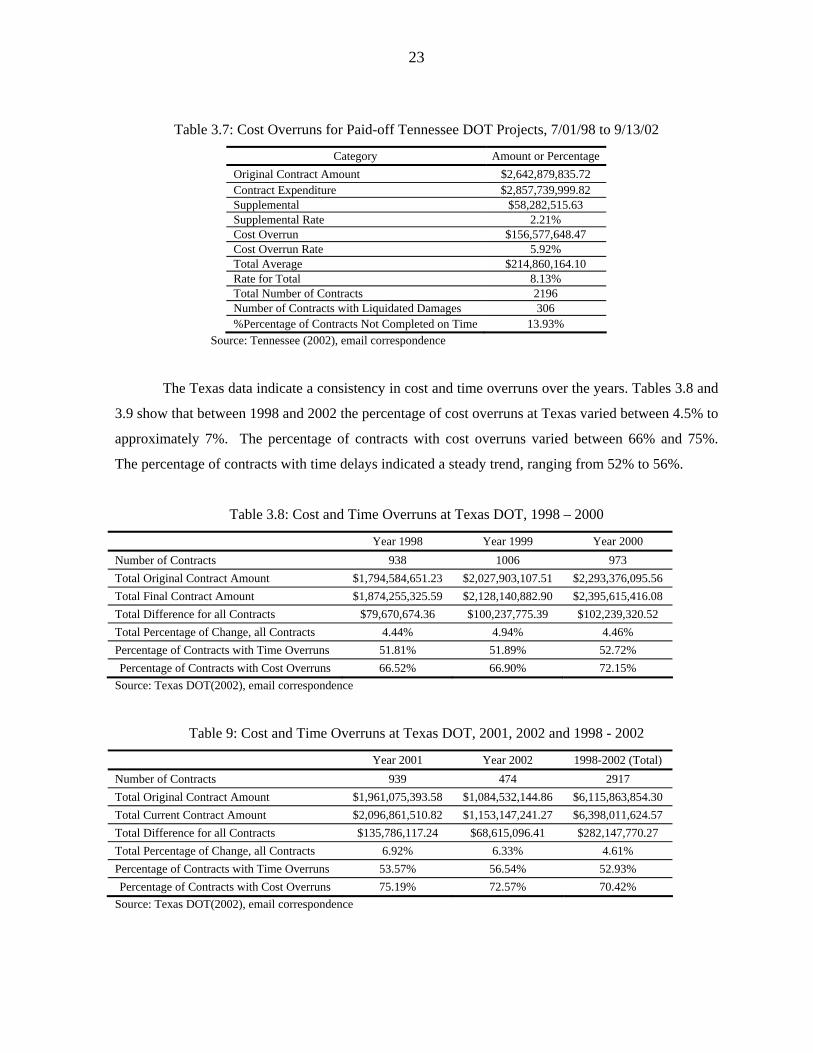
23
Table 3.7: Cost Overruns for Paid-off Tennessee DOT Projects, 7/01/98 to 9/13/02
Category Amount or Percentage Original Contract Amount $2,642,879,835.72 Contract Expenditure $2,857,739,999.82 Supplemental $58,282,515.63 Supplemental Rate 2.21% Cost Overrun $156,577,648.47 Cost Overrun Rate 5.92% Total Average $214,860,164.10 Rate for Total 8.13% Total Number of Contracts 2196 Number of Contracts with Liquidated Damages 306 %Percentage of Contracts Not Completed on Time 13.93%
Source: Tennessee (2002), email correspondence
The Texas data indicate a consistency in cost and time overruns over the years. Tables 3.8 and
3.9 show that between 1998 and 2002 the percentage of cost overruns at Texas varied between 4.5% to
approximately 7%. The percentage of contracts with cost overruns varied between 66% and 75%.
The percentage of contracts with time delays indicated a steady trend, ranging from 52% to 56%.
Table 3.8: Cost and Time Overruns at Texas DOT, 1998 – 2000
Year 1998 Year 1999 Year 2000 Number of Contracts 938 1006 973 Total Original Contract Amount $1,794,584,651.23 $2,027,903,107.51 $2,293,376,095.56 Total Final Contract Amount $1,874,255,325.59 $2,128,140,882.90 $2,395,615,416.08 Total Difference for all Contracts $79,670,674.36 $100,237,775.39 $102,239,320.52 Total Percentage of Change, all Contracts 4.44% 4.94% 4.46% Percentage of Contracts with Time Overruns 51.81% 51.89% 52.72% Percentage of Contracts with Cost Overruns 66.52% 66.90% 72.15%
Source: Texas DOT(2002), email correspondence
Table 9: Cost and Time Overruns at Texas DOT, 2001, 2002 and 1998 - 2002
Year 2001 Year 2002 1998-2002 (Total) Number of Contracts 939 474 2917 Total Original Contract Amount $1,961,075,393.58 $1,084,532,144.86 $6,115,863,854.30 Total Current Contract Amount $2,096,861,510.82 $1,153,147,241.27 $6,398,011,624.57 Total Difference for all Contracts $135,786,117.24 $68,615,096.41 $282,147,770.27 Total Percentage of Change, all Contracts 6.92% 6.33% 4.61% Percentage of Contracts with Time Overruns 53.57% 56.54% 52.93% Percentage of Contracts with Cost Overruns 75.19% 72.57% 70.42%
Source: Texas DOT(2002), email correspondence
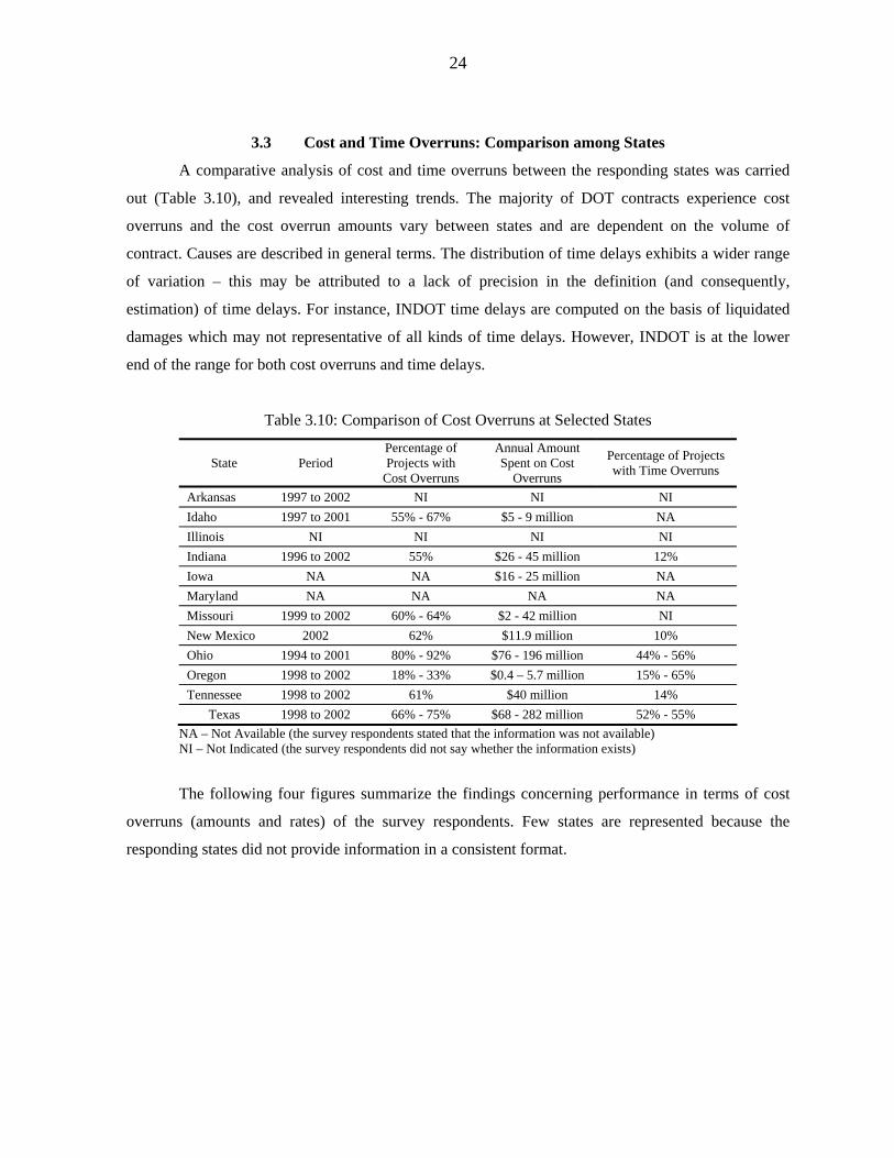
24
3.3 Cost and Time Overruns: Comparison among States
A comparative analysis of cost and time overruns between the responding states was carried
out (Table 3.10), and revealed interesting trends. The majority of DOT contracts experience cost
overruns and the cost overrun amounts vary between states and are dependent on the volume of
contract. Causes are described in general terms. The distribution of time delays exhibits a wider range
of variation – this may be attributed to a lack of precision in the definition (and consequently,
estimation) of time delays. For instance, INDOT time delays are computed on the basis of liquidated
damages which may not representative of all kinds of time delays. However, INDOT is at the lower
end of the range for both cost overruns and time delays.
Table 3.10: Comparison of Cost Overruns at Selected States
State Period Percentage of Projects with
Cost Overruns
Annual Amount Spent on Cost
Overruns
Percentage of Projects with Time Overruns
Arkansas 1997 to 2002 NI NI NI Idaho 1997 to 2001 55% - 67% $5 - 9 million NA Illinois NI NI NI NI Indiana 1996 to 2002 55% $26 - 45 million 12% Iowa NA NA $16 - 25 million NA Maryland NA NA NA NA Missouri 1999 to 2002 60% - 64% $2 - 42 million NI New Mexico 2002 62% $11.9 million 10% Ohio 1994 to 2001 80% - 92% $76 - 196 million 44% - 56% Oregon 1998 to 2002 18% - 33% $0.4 – 5.7 million 15% - 65% Tennessee 1998 to 2002 61% $40 million 14%
Texas 1998 to 2002 66% - 75% $68 - 282 million 52% - 55% NA – Not Available (the survey respondents stated that the information was not available) NI – Not Indicated (the survey respondents did not say whether the information exists)
The following four figures summarize the findings concerning performance in terms of cost
overruns (amounts and rates) of the survey respondents. Few states are represented because the
responding states did not provide information in a consistent format.
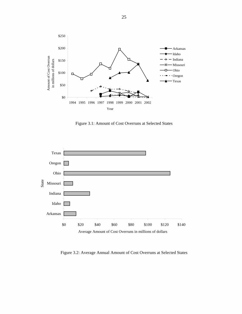
25
$0
$50
$100
$150
$200
$250
1994 1995 1996 1997 1998 1999 2000 2001 2002
Year
Am
ount
of C
ost O
verr
un
in m
illio
ns o
f dol
lars
ArkansasIdahoIndianaMissouriOhioOregonTexas
Figure 3.1: Amount of Cost Overruns at Selected States
$0 $20 $40 $60 $80 $100 $120 $140
Arkansas
Idaho
Indiana
Missouri
Ohio
Oregon
Texas
Stat
e
Average Amount of Cost Overruns in millions of dollars
Figure 3.2: Average Annual Amount of Cost Overruns at Selected States
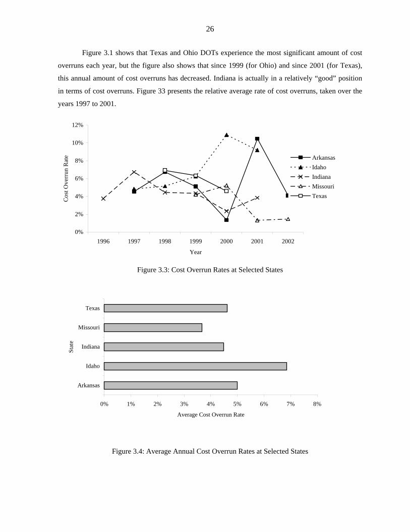
26
Figure 3.1 shows that Texas and Ohio DOTs experience the most significant amount of cost
overruns each year, but the figure also shows that since 1999 (for Ohio) and since 2001 (for Texas),
this annual amount of cost overruns has decreased. Indiana is actually in a relatively “good” position
in terms of cost overruns. Figure 33 presents the relative average rate of cost overruns, taken over the
years 1997 to 2001.
0%
2%
4%
6%
8%
10%
12%
1996 1997 1998 1999 2000 2001 2002
Year
Cos
t Ove
rrun
Rat
e ArkansasIdahoIndianaMissouriTexas
Figure 3.3: Cost Overrun Rates at Selected States
0% 1% 2% 3% 4% 5% 6% 7% 8%
Arkansas
Idaho
Indiana
Missouri
Texas
Stat
e
Average Cost Overrun Rate
Figure 3.4: Average Annual Cost Overrun Rates at Selected States
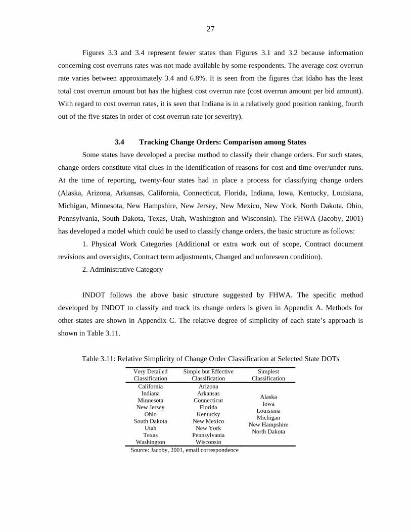
27
Figures 3.3 and 3.4 represent fewer states than Figures 3.1 and 3.2 because information
concerning cost overruns rates was not made available by some respondents. The average cost overrun
rate varies between approximately 3.4 and 6.8%. It is seen from the figures that Idaho has the least
total cost overrun amount but has the highest cost overrun rate (cost overrun amount per bid amount).
With regard to cost overrun rates, it is seen that Indiana is in a relatively good position ranking, fourth
out of the five states in order of cost overrun rate (or severity).
3.4 Tracking Change Orders: Comparison among States
Some states have developed a precise method to classify their change orders. For such states,
change orders constitute vital clues in the identification of reasons for cost and time over/under runs.
At the time of reporting, twenty-four states had in place a process for classifying change orders
(Alaska, Arizona, Arkansas, California, Connecticut, Florida, Indiana, Iowa, Kentucky, Louisiana,
Michigan, Minnesota, New Hampshire, New Jersey, New Mexico, New York, North Dakota, Ohio,
Pennsylvania, South Dakota, Texas, Utah, Washington and Wisconsin). The FHWA (Jacoby, 2001)
has developed a model which could be used to classify change orders, the basic structure as follows:
1. Physical Work Categories (Additional or extra work out of scope, Contract document
revisions and oversights, Contract term adjustments, Changed and unforeseen condition).
2. Administrative Category
INDOT follows the above basic structure suggested by FHWA. The specific method
developed by INDOT to classify and track its change orders is given in Appendix A. Methods for
other states are shown in Appendix C. The relative degree of simplicity of each state’s approach is
shown in Table 3.11.
Table 3.11: Relative Simplicity of Change Order Classification at Selected State DOTs
Very Detailed Classification
Simple but Effective Classification
Simplest Classification
California Indiana
Minnesota New Jersey
Ohio South Dakota
Utah Texas
Washington
Arizona Arkansas
Connecticut Florida
Kentucky New Mexico
New York Pennsylvania
Wisconsin
Alaska Iowa
Louisiana Michigan
New Hampshire North Dakota
Source: Jacoby, 2001, email correspondence
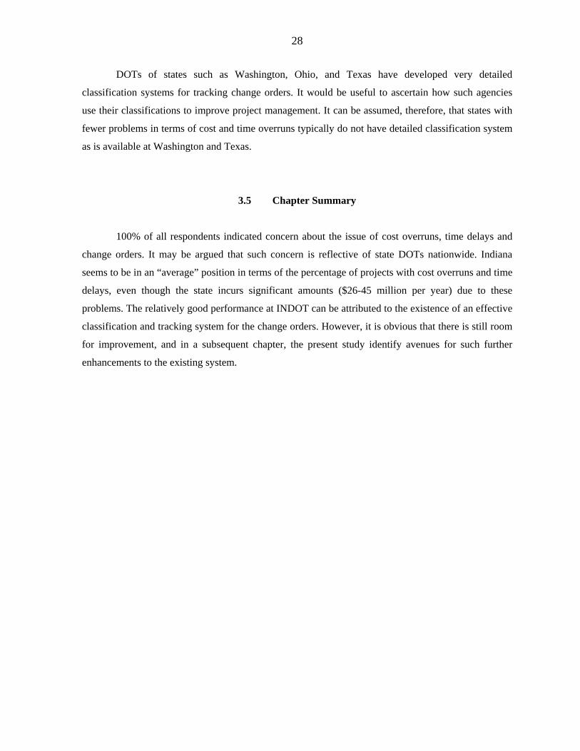
28
DOTs of states such as Washington, Ohio, and Texas have developed very detailed
classification systems for tracking change orders. It would be useful to ascertain how such agencies
use their classifications to improve project management. It can be assumed, therefore, that states with
fewer problems in terms of cost and time overruns typically do not have detailed classification system
as is available at Washington and Texas.
3.5 Chapter Summary
100% of all respondents indicated concern about the issue of cost overruns, time delays and
change orders. It may be argued that such concern is reflective of state DOTs nationwide. Indiana
seems to be in an “average” position in terms of the percentage of projects with cost overruns and time
delays, even though the state incurs significant amounts ($26-45 million per year) due to these
problems. The relatively good performance at INDOT can be attributed to the existence of an effective
classification and tracking system for the change orders. However, it is obvious that there is still room
for improvement, and in a subsequent chapter, the present study identify avenues for such further
enhancements to the existing system.
29
CHAPTER 4: STUDY METHODOLOGY
4.1 Introduction
This chapter explains the overall framework, methods, and underlying assumptions for
analyzing the problem of cost overruns, time delays and change orders in Indiana. Figure 4.1 presents
an overview of the steps. The methodology includes preliminary descriptive statistics that examines
the general temporal and spatial trends in the data. It also includes correlation matrix analysis, pair-
wise tests, analysis of variance, and statistical modeling. The methodologies include definitions of
dependent variables (cost overrun amounts and rates, time delay and change orders) and potential
influential factors (independent variables), and selection of model categories and appropriate
mathematical forms. Also, techniques used for model calibration and validation are discussed in the
present chapter. The methodology was designed to yield statistical models with a view to predict cost
overruns and time delays, but more importantly, to identify significant factors that influence cost
overruns, time delays and the frequency of change orders.
4.2 Descriptive Statistics
The present study seeks to identify the main reasons and responsibilities for change orders,
among others, and it is expected that a descriptive statistical analysis would throw more light on this
issue. For cost overruns and time delays, descriptive statistical analysis in terms of their frequency
and amounts was carried out. Simple descriptive graphs (histograms) may show any variations in such
attributes by geographical location, type of project or year of implementation. Moreover, descriptive
figures such as pie charts easily and readily show the relative significance of various categories of cost
overruns. A description of the distribution and frequency of each type of change order can help
understanding the extents and root causes of the problem.
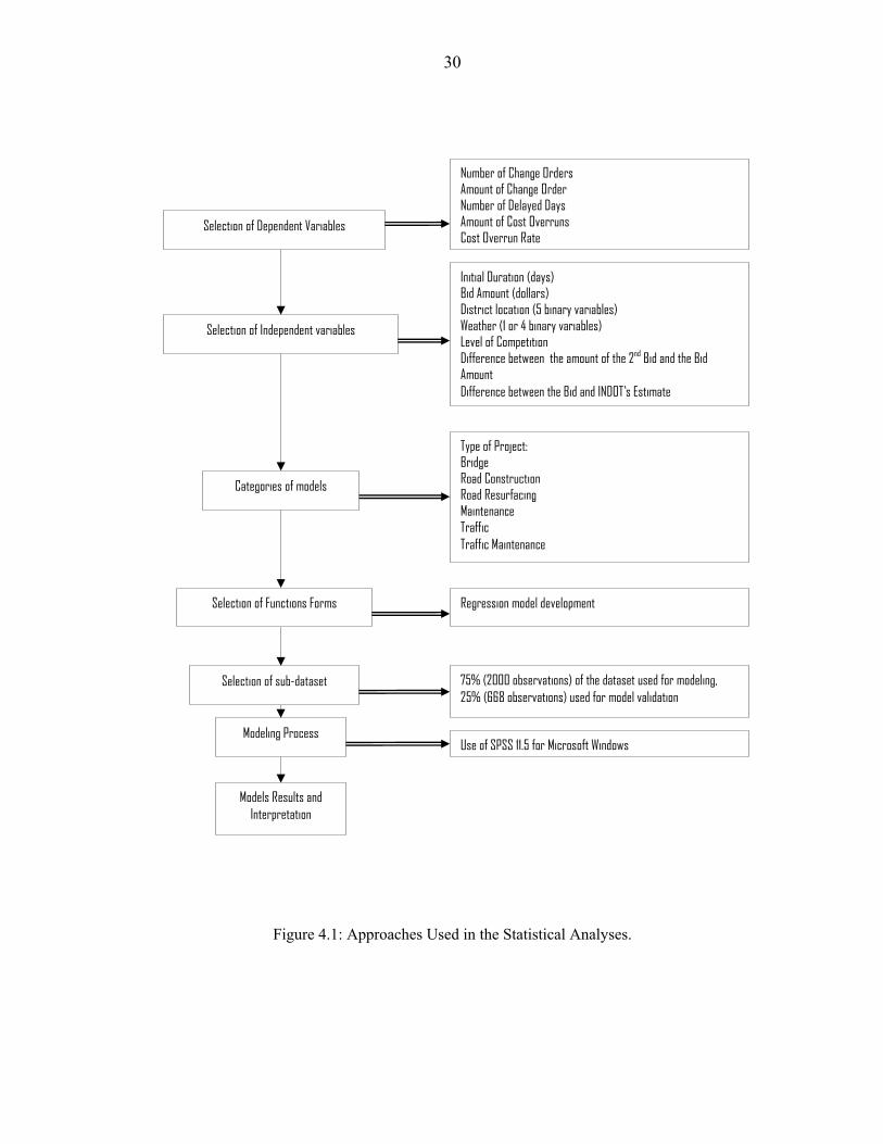
30
Figure 4.1: Approaches Used in the Statistical Analyses.
Selection of Dependent Variables
Selection of Independent variables
Number of Change Orders Amount of Change Order Number of Delayed Days Amount of Cost Overruns Cost Overrun Rate
Initial Duration (days) Bid Amount (dollars) District location (5 binary variables) Weather (1 or 4 binary variables) Level of Competition Difference between the amount of the 2nd Bid and the Bid Amount Difference between the Bid and INDOT’s Estimate
Modeling Process
Selection of sub-dataset
Models Results and Interpretation
Selection of Functions Forms Regression model development
75% (2000 observations) of the dataset used for modeling, 25% (668 observations) used for model validation
Use of SPSS 11.5 for Microsoft Windows
Type of Project: Bridge Road Construction Road Resurfacing Maintenance Traffic Traffic Maintenance
Categories of models
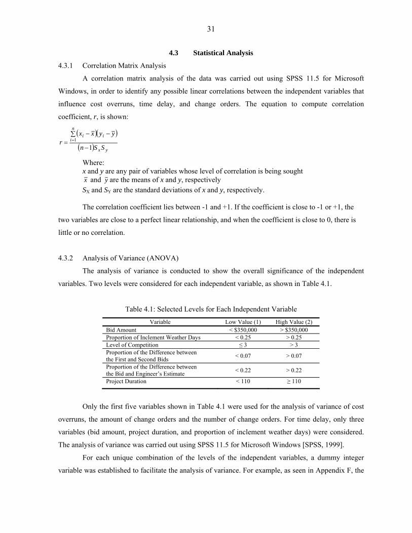
31
4.3 Statistical Analysis
4.3.1 Correlation Matrix Analysis
A correlation matrix analysis of the data was carried out using SPSS 11.5 for Microsoft
Windows, in order to identify any possible linear correlations between the independent variables that
influence cost overruns, time delay, and change orders. The equation to compute correlation
coefficient, r, is shown:
( )( )
( ) yx
n
iii
SSn
yyxxr
11
−
∑ −−= =
Where: x and y are any pair of variables whose level of correlation is being sought x and y are the means of x and y, respectively SX and SY are the standard deviations of x and y, respectively.
The correlation coefficient lies between -1 and +1. If the coefficient is close to -1 or +1, the
two variables are close to a perfect linear relationship, and when the coefficient is close to 0, there is
little or no correlation.
4.3.2 Analysis of Variance (ANOVA)
The analysis of variance is conducted to show the overall significance of the independent
variables. Two levels were considered for each independent variable, as shown in Table 4.1.
Table 4.1: Selected Levels for Each Independent Variable
Variable Low Value (1) High Value (2) Bid Amount < $350,000 > $350,000 Proportion of Inclement Weather Days < 0.25 > 0.25 Level of Competition ≤ 3 > 3 Proportion of the Difference between the First and Second Bids < 0.07 > 0.07
Proportion of the Difference between the Bid and Engineer’s Estimate < 0.22 > 0.22
Project Duration < 110 ≥ 110
Only the first five variables shown in Table 4.1 were used for the analysis of variance of cost
overruns, the amount of change orders and the number of change orders. For time delay, only three
variables (bid amount, project duration, and proportion of inclement weather days) were considered.
The analysis of variance was carried out using SPSS 11.5 for Microsoft Windows [SPSS, 1999].
For each unique combination of the levels of the independent variables, a dummy integer
variable was established to facilitate the analysis of variance. For example, as seen in Appendix F, the
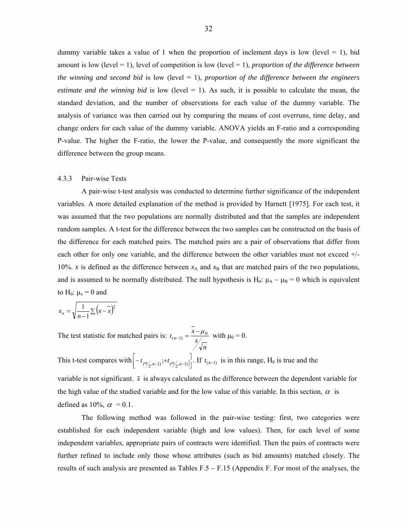
32
dummy variable takes a value of 1 when the proportion of inclement days is low (level = 1), bid
amount is low (level = 1), level of competition is low (level = 1), proportion of the difference between
the winning and second bid is low (level = 1), proportion of the difference between the engineers
estimate and the winning bid is low (level = 1). As such, it is possible to calculate the mean, the
standard deviation, and the number of observations for each value of the dummy variable. The
analysis of variance was then carried out by comparing the means of cost overruns, time delay, and
change orders for each value of the dummy variable. ANOVA yields an F-ratio and a corresponding
P-value. The higher the F-ratio, the lower the P-value, and consequently the more significant the
difference between the group means.
4.3.3 Pair-wise Tests
A pair-wise t-test analysis was conducted to determine further significance of the independent
variables. A more detailed explanation of the method is provided by Harnett [1975]. For each test, it
was assumed that the two populations are normally distributed and that the samples are independent
random samples. A t-test for the difference between the two samples can be constructed on the basis of
the difference for each matched pairs. The matched pairs are a pair of observations that differ from
each other for only one variable, and the difference between the other variables must not exceed +/-
10%. x is defined as the difference between xA and xB that are matched pairs of the two populations,
and is assumed to be normally distributed. The null hypothesis is H0: µA – µB = 0 which is equivalent
to H0: µx = 0 and
( )∑ −−
=2
11 xx
nsx
The test statistic for matched pairs is: n
sx
t n0
)1(µ−
=− with µ0 = 0.
This t-test compares with ⎥⎦⎤
⎢⎣⎡ +−
−− )1,2()1,2( ; nn tt αα . If )1( −nt is in this range, H0 is true and the
variable is not significant. x is always calculated as the difference between the dependent variable for
the high value of the studied variable and for the low value of this variable. In this section, α is
defined as 10%, α = 0.1.
The following method was followed in the pair-wise testing: first, two categories were
established for each independent variable (high and low values). Then, for each level of some
independent variables, appropriate pairs of contracts were identified. Then the pairs of contracts were
further refined to include only those whose attributes (such as bid amounts) matched closely. The
results of such analysis are presented as Tables F.5 – F.15 (Appendix F. For most of the analyses, the
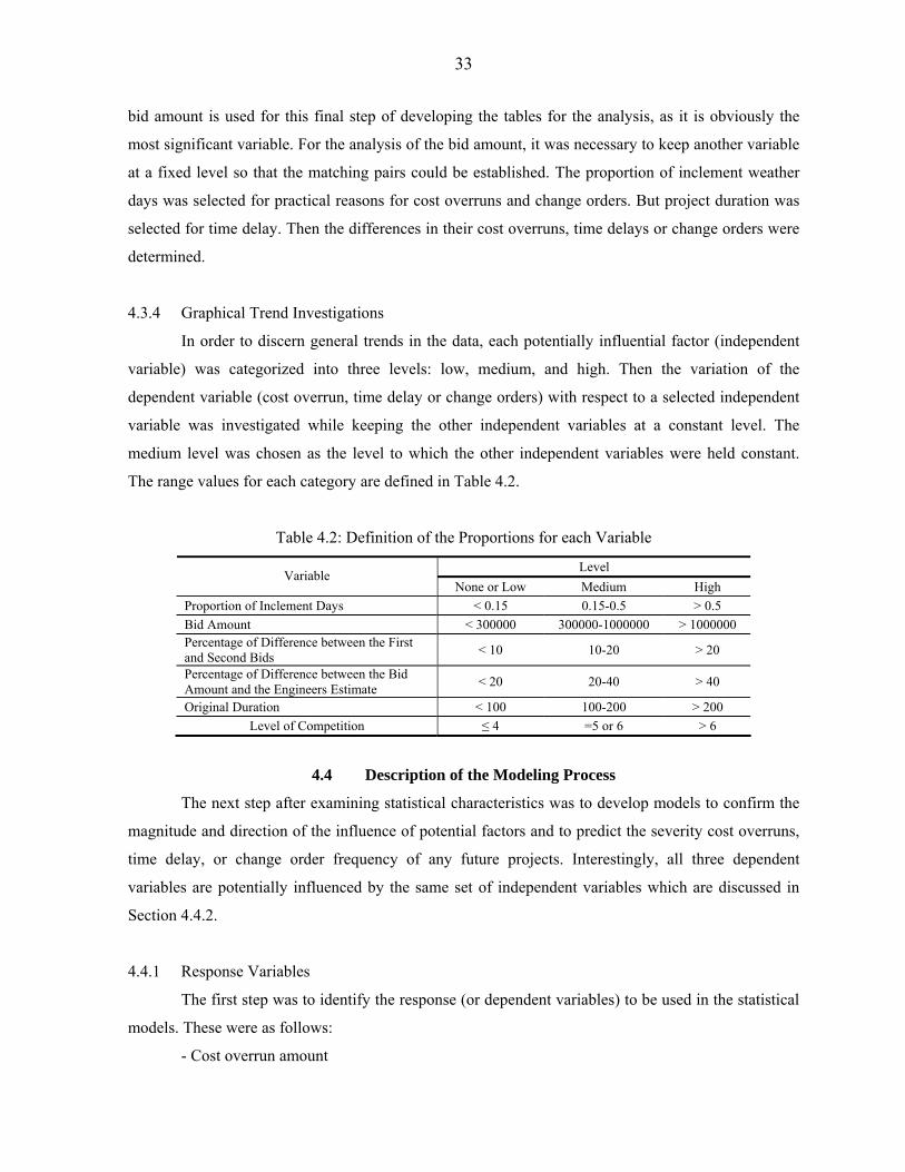
33
bid amount is used for this final step of developing the tables for the analysis, as it is obviously the
most significant variable. For the analysis of the bid amount, it was necessary to keep another variable
at a fixed level so that the matching pairs could be established. The proportion of inclement weather
days was selected for practical reasons for cost overruns and change orders. But project duration was
selected for time delay. Then the differences in their cost overruns, time delays or change orders were
determined.
4.3.4 Graphical Trend Investigations
In order to discern general trends in the data, each potentially influential factor (independent
variable) was categorized into three levels: low, medium, and high. Then the variation of the
dependent variable (cost overrun, time delay or change orders) with respect to a selected independent
variable was investigated while keeping the other independent variables at a constant level. The
medium level was chosen as the level to which the other independent variables were held constant.
The range values for each category are defined in Table 4.2.
Table 4.2: Definition of the Proportions for each Variable
Level Variable
None or Low Medium High Proportion of Inclement Days < 0.15 0.15-0.5 > 0.5 Bid Amount < 300000 300000-1000000 > 1000000 Percentage of Difference between the First and Second Bids < 10 10-20 > 20
Percentage of Difference between the Bid Amount and the Engineers Estimate < 20 20-40 > 40
Original Duration < 100 100-200 > 200 Level of Competition ≤ 4 =5 or 6 > 6
4.4 Description of the Modeling Process
The next step after examining statistical characteristics was to develop models to confirm the
magnitude and direction of the influence of potential factors and to predict the severity cost overruns,
time delay, or change order frequency of any future projects. Interestingly, all three dependent
variables are potentially influenced by the same set of independent variables which are discussed in
Section 4.4.2.
4.4.1 Response Variables
The first step was to identify the response (or dependent variables) to be used in the statistical
models. These were as follows:
- Cost overrun amount
34
- Cost overrun rate (cost overrun amount divided by the bid amount)
- Time delay (in days)
- Number of change orders
- Amount of change orders
4.4.1.1 Cost Overrun
The total amount of cost overrun was calculated by the difference between the final contract
cost and the bid amount. In another set of models the response variables was the cost overrun rate,
which is the percent difference in cost (positive or negative) between the final contract cost and the
contract award amount (Jahren and Ashe, 1990).
4.4.1.2 Time Delay
The response variable for the time delay models was the number of days of time overrun,
which is defined as the difference between the actual duration of the project and the original duration
(decided in the contract). The dataset provided the following dates: the notice to proceed date, the last
day of work, and the estimated date of project completion, which enabled calculation of the time
delay.
4.4.1.3 Change Orders
There were two types of change order information: the daily change order that contains all the
change orders in a day and the second type is the member of individual change orders. In the present
study, the number of individual change orders, as well as the total amount of money involved in
change order, was modeled as a function of various independent variables.
4.4.2 Independent Variables
The second step was to identify the factors that potentially influence the amount of change
orders, cost overruns and time delays. This step was guided by the findings from the literature review
and agency survey (Chapter 2 and 3). The results of the descriptive statistics, pair-wise t test and
analysis of variance were instrumental in developing a tentative list of independent variables for use in
the statistical models.
An important independent variable is project duration, or the initial length (days) of the
project, computed as the difference between the estimated last day of work and the notice to proceed
date. An initial expectation for this variable would be that longer projects would result in longer
delays. Indeed, Rowland [1981] found that the size of the project is a significant variable. Size can be
35
understood as the total cost or duration of the project. It is intuitive that a high-cost project will likely
involve a long contract duration. Conversely, a project of long duration is likely to have a high cost.
So, these two potential influential variables are obviously related to each other. Rowland [1981] states
that a bigger project would have a greater change order amount rate. In the present study, the initial
project length was used only for time delay models because this is the most relevant variable for these
models.
The bid amount (in dollars) may also be a significant variable for all three model types. It is
quite possible that correlation may exist between the bid amount variable and the initial length (days).
The project size in terms of cost and the size in terms of length may exhibit different levels of
influence on the dependent variables. On one hand, it can be hypothesized that an expensive project is
often managed more efficiently, resulting in less delay. On the other hand, it may be argued that the
involvement of more contractors and subcontractors may result in increased delay certainly because of
inevitable lapses in communication between them. The same comment can be made about the impact
of project size on cost overrun.
To examine the influence of project type, six binary variables were created (bridge, road
construction, resurfacing, maintenance, traffic, and traffic maintenance). Each of these variables takes
a value of 1 if the information pertains to the project type, 0 otherwise. Bridge and road construction
projects may not suffer from traffic management as much as the other projects, so there may be less
risk in terms of safety and delay. However, actual bridge construction is much more unpredictable
than the other project types, and unforeseen site conditions or delays in obtaining right-of-way could
cause delays and cost overruns. Maintenance and traffic projects are significantly affected by passing
traffic, but overall, a lower level of construction delays and cost overruns may be expected for such
projects because of their typical small size and short duration. Jahren and Ashe [1990] found that the
size of a project is significant in time delays. For models that included the “project type” variable, five
binary variables were used (excluding the traffic maintenance variable). As such, a project that shows
a zero value for all the binary variables is a traffic maintenance project.
The district at which a project is located may be a significant variable because of variations in
weather and administrative practices/culture. Contract locations by districts were represented using
binary variables. It is possible that some interaction may exist between the variables representing
contract location and those representing weather conditions. The district variables are expected to
reveal differences in the effectiveness of supervision practices. If these variables are found to be
strongly related to the weather variables, they may only represent a climatic and geological variation
among the state. However, if this is not the case, other disparities may be revealed among the districts,
36
such as INDOT staff’s management efficiency, the performance of the main contractors in the district,
etc.
Weather variation was not considered in previous studies. In the present study, four different
continuous variables were used to describe the weather conditions during the duration of each project.
- Temperature (in number of days with a temperature less than 0 degree Celsius)
- Rain precipitation (in number of days with rain precipitation)
- Snow precipitation (in number of days with snow precipitation)
- Ground snow conditions (in number of days with snow on the ground)
These variables are expected to reveal the impact of inclement weather conditions on the
construction process. It is expected that the coefficients for these variables will have a positive sign for
all models. In order to prevent correlation between the four weather variables, another independent
variable was considered: inclement weather (in terms of the number of days of the contract duration
that experienced either low temperature (less than zero degree Celsius), precipitation, snow, or snow
on the ground). This new variable incorporates the four weather variables. It helps avoid the problems
of correlation because when the temperature is under zero degree Celsius, any precipitation will be in
the form of snow, not rain. The same comment can be made for the variable “ground snow
conditions,” because it is obviously strongly related to the variable “snow precipitation.” These
weather variables (expressed in the number of days) are finally reduced to a rate by dividing the
number of inclement days by the total number of days worked on the project.
The level of competition for each contract is the number of contractors who submitted a bid to
INDOT for that contract. The level of competition was found relevant in the Jahren and Ashe [1990]
study. Obviously, it is expected that the higher the level of competition, the more competitive the
bidding, and consequently the higher the number of change orders, cost overruns and time delays
likely to be experienced by the contract.
The difference between the bid amount and the INDOT engineer’s estimate was also taken
into account in the present study to ascertain the validity of Rowland’s assertion [1981] that the larger
the absolute value of the difference between the owner’s fair cost estimate and the low bid on a
project, the greater the likelihood that a job will experience more change orders, and by extension,
more cost overruns.
The difference between the bid amount and the next low bid might have an influence on the
number of change orders as found by Rowland [1981]. It is expected that when such difference is
larger, the number of change orders or cost overrun amounts is greater.
For these variables (i.e., the difference between the first and second bids and between the bid
and the engineer’s estimate) a rate is defined by dividing these amounts by the original bid amount.
37
4.4.3 Project Types
The project type variable was deemed appropriate for categorizing the statistical analyses. The
categories consisting of bridge, road construction, resurfacing, maintenance, traffic and traffic
maintenance are characterized by significant differences in management practices due to the nature of
the categories. Separate models were developed for each category. Also, a general model for all
contracts that utilized project type independent variables (rather than having model families based on
project type) was developed to further investigate any differences between the impacts of each project
type.
4.4.4 Investigation and Selection of Mathematical Forms
All the variables were modeled with the linear regression form, and some typical Box Cox
transformations were tried for each dependent variable, depending on the range of these variables.
4.4.5 Model Calibration and Validation
Influential variables were selected on the basis of their relatively high statistical significance,
which was ascertained using their t-statistics and P-values given with the model results. The best
models were obtained through progressive inclusion and exclusion of various variables in the models.
The variables were selected or inclusion if their t-statistics were approximately greater than 1.6. The
statistical package SPSS 11.5 for Windows [SPSS, 1999] was used to run the regressions.
Approximately 25% of the data was set aside to validate the models. As such, of the 2,668
projects, a randomly selected set of 2,000 projects were used for the modeling process. The other set
of 668 projects were used to determine whether the predictions given by the calibrated model matched
the observed values. The following parameters were estimated to evaluate the effectiveness of each
model:
Root mean square error = ( )n
xxobs∑ − 2mod
Percentage of deviations = ∑−
obs
obs
xxx mod
38
4.5 Chapter Summary
The present chapter explained the overall framework, methods, and underlying assumptions
for analyzing the problem of cost overruns, time delays and change orders in Indiana. The
methodology included preliminary descriptive statistics, correlation matrix analysis, pair-wise t tests,
analysis of variance, and statistical modeling. The chapter provided a description of the methodologies
used in the statistical analysis. Five models types, based on the form of response variable, were
considered for development: number of change orders, change order amount, severity of time overrun,
cost overrun, and cost overrun rate. The following independent variables were discussed: duration, bid
amount, project type, district, weather conditions, level of competition, engineer’s estimate
comparison, and first and second bid comparison. Also, appropriate functional forms were discussed.
The techniques used for model calibration and validation were also discussed in the present chapter.
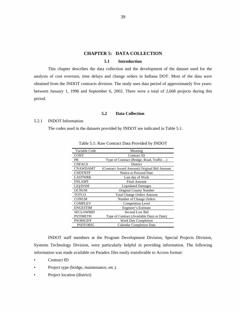
39
CHAPTER 5: DATA COLLECTION
5.1 Introduction
This chapter describes the data collection and the development of the dataset used for the
analysis of cost overruns, time delays and change orders in Indiana DOT. Most of the data were
obtained from the INDOT contracts division. The study uses data period of approximately five years:
between January 1, 1996 and September 6, 2002. There were a total of 2,668 projects during this
period.
5.2 Data Collection
5.2.1 INDOT Information
The codes used in the datasets provided by INDOT are indicated in Table 5.1.
Table 5.1: Raw Contract Data Provided by INDOT
Variable Code Meaning CONT Contract ID PR Type of Contract (Bridge, Road, Traffic…) CNFACS District CNAWDAMT (Contract Award Amount) Original Bid Amount CNDTNTP Notice to Proceed Date LASTWRK Last day of Work FNLAMT Final Amount LIQ/DAM Liquidated Damages OCNUM Original County Number TOTCO Total Change Orders Amount CONUM Number of Change Orders COMPLEV Competition Level ENGESTIM Engineer’s Estimate SECLOWBID PSTIMETH
Second Low Bid Type of Contract (Available Days or Date)
PSORIGDY Work Day Completion PSDTORIG Calendar Completion Date
INDOT staff members at the Program Development Division, Special Projects Division,
Systems Technology Division, were particularly helpful in providing information. The following
information was made available on Paradox files easily transferable to Access format:
• Contract ID
• Project type (bridge, maintenance, etc.)
• Project location (district)
40
• Bid amount
• Final amount
• Dates: Notice to proceed, Acceptance date, Final day of work.
• Liquidated damages
Most of this information is also available at the following website:
http://www.in.gov/dot/div/contracts/letting/oldletting.html, which is regularly updated. The data
concerning the level of competition, the engineer’s estimate, and the second low bid was also obtained
from this website. The following information on change orders was made available in Access format:
• Description of each change order
• Reason code
• Amount of change orders in dollars
• Expected final date
The following information was provided in Excel files that were exported from BAM files:
• Project location (counties, in order to introduce the weather data into the dataset)
• Amount of change orders in dollars
• Vendor’s reference
• Description of the location
A portion of the data could not be used because of a lack of explanation of the codes used in
the dataset supplied by INDOT. In some cases, many columns were empty.
Figure 5.1 indicates the geographical location of the various INDOT districts in Indiana. The
present study takes into account data from these six districts: La Porte, Fort Wayne, Crawfordsville,
Greenfield, Seymour, and Vincennes. The Toll Road district is not represented because no contract
data was provided on this district for this study.

41
Figure 5.1: Highway Administrative Districts in Indiana
Data regarding change order reasons were not incorporated into the main dataset because they
had to be organized differently. The available data provided for each contract a description of each
change order: contract number, unit price, quantity, and reason for the change order (code). The final
cost of the change order (obtained by multiplying the quantity by the unit price) and the reason for the
change order are the most important pieces of information. For this database, six major datasets were
created for each project type (bridge, maintenance, etc) and seven different descriptions were done in
order to compare the different categories of work in terms of responsibility for change orders. For the
analysis, the number of change orders and the amounts of the change orders for a given contract were
incorporated in the main dataset.
42
5.2.2 Weather Data
The weather data were available on the web site: http://shadow.agry.purdue.edu/sc.index.html.
The county-specific data covered the period between January 1, 1995 and November 1, 2002. The
following data were collected:
- Maximum temperature
- Minimum temperature
- Amount of rainfall in inches
- Amount of snowfall in inches only between November and March
- Amount of snow on the ground in inches
5.3 Database Development
5.3.1 Refinement of the Dataset
Contracts with incomplete information because of errors or missing data were deleted from the
modeling dataset. Consequently, the dataset used for the three types of models (cost overruns, time
delays, and change orders) were slightly different. Moreover, there were a few potentially influential
factors (independent variables) for which available data did not cover the entire dataset. As such, it
was found prudent to develop two sets of models: one with the entire dataset but with few variables,
and the another with a reduced dataset but with many variables. Also, a few outliers were excluded
form the modeling dataset,
5.3.2 Weather Database
The present study placed more emphasis on the number of inclement weather days compared
to the actual amount of daily precipitation. Therefore, for the duration of each contract, the number of
days (with rain, snow, or cold days) was counted. It considered that snow and rain not only preclude a
day of work, but also cause the entire process of construction to slow down. The data collection was
subsequently simplified In the dataset, weather conditions are presented as the number of days with
the following attributes:
- cold temperatures. Cold days were defined with maximum temperature under zero degree
Celsius, i.e., 32 degrees Fahrenheit
- rain precipitation
- snow precipitation
- snow on the ground
Information from Figure 5.2 was used in inputting missing weather data by utilizing data from
the closest county that had weather data (Appendix D). For a few counties with missing data, the
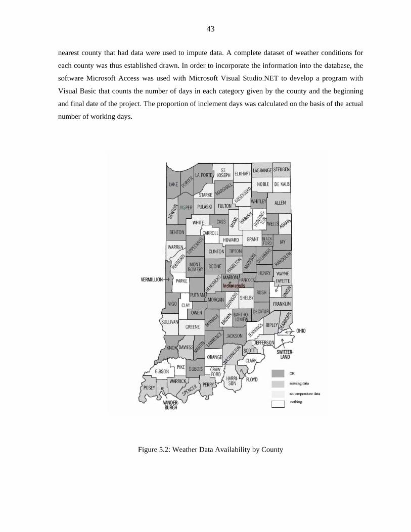
43
nearest county that had data were used to impute data. A complete dataset of weather conditions for
each county was thus established drawn. In order to incorporate the information into the database, the
software Microsoft Access was used with Microsoft Visual Studio.NET to develop a program with
Visual Basic that counts the number of days in each category given by the county and the beginning
and final date of the project. The proportion of inclement days was calculated on the basis of the actual
number of working days.
Figure 5.2: Weather Data Availability by County
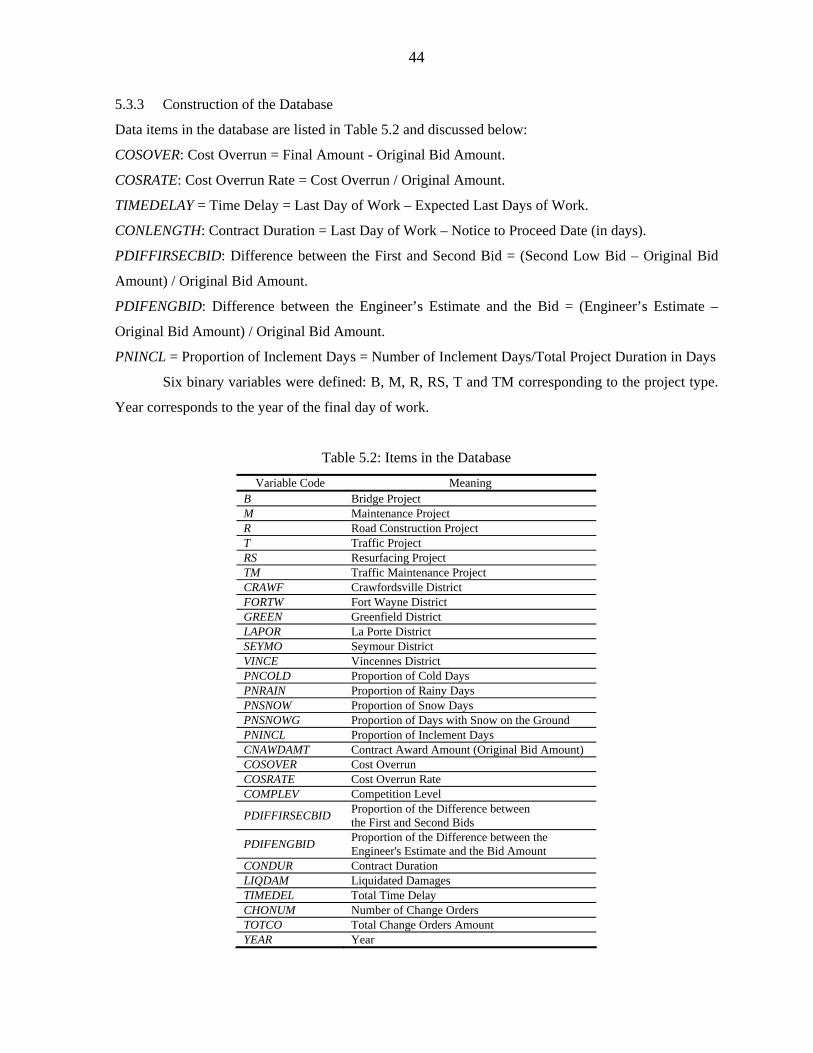
44
5.3.3 Construction of the Database
Data items in the database are listed in Table 5.2 and discussed below:
COSOVER: Cost Overrun = Final Amount - Original Bid Amount.
COSRATE: Cost Overrun Rate = Cost Overrun / Original Amount.
TIMEDELAY = Time Delay = Last Day of Work – Expected Last Days of Work.
CONLENGTH: Contract Duration = Last Day of Work – Notice to Proceed Date (in days).
PDIFFIRSECBID: Difference between the First and Second Bid = (Second Low Bid – Original Bid
Amount) / Original Bid Amount.
PDIFENGBID: Difference between the Engineer’s Estimate and the Bid = (Engineer’s Estimate –
Original Bid Amount) / Original Bid Amount.
PNINCL = Proportion of Inclement Days = Number of Inclement Days/Total Project Duration in Days
Six binary variables were defined: B, M, R, RS, T and TM corresponding to the project type.
Year corresponds to the year of the final day of work.
Table 5.2: Items in the Database
Variable Code Meaning B Bridge Project M Maintenance Project R Road Construction Project T Traffic Project RS Resurfacing Project TM Traffic Maintenance Project CRAWF Crawfordsville District FORTW Fort Wayne District GREEN Greenfield District LAPOR La Porte District SEYMO Seymour District VINCE Vincennes District PNCOLD Proportion of Cold Days PNRAIN Proportion of Rainy Days PNSNOW Proportion of Snow Days PNSNOWG Proportion of Days with Snow on the Ground PNINCL Proportion of Inclement Days CNAWDAMT Contract Award Amount (Original Bid Amount) COSOVER Cost Overrun COSRATE Cost Overrun Rate COMPLEV Competition Level
PDIFFIRSECBID Proportion of the Difference between the First and Second Bids
PDIFENGBID Proportion of the Difference between the Engineer's Estimate and the Bid Amount
CONDUR Contract Duration LIQDAM Liquidated Damages TIMEDEL Total Time Delay CHONUM Number of Change Orders TOTCO Total Change Orders Amount YEAR Year
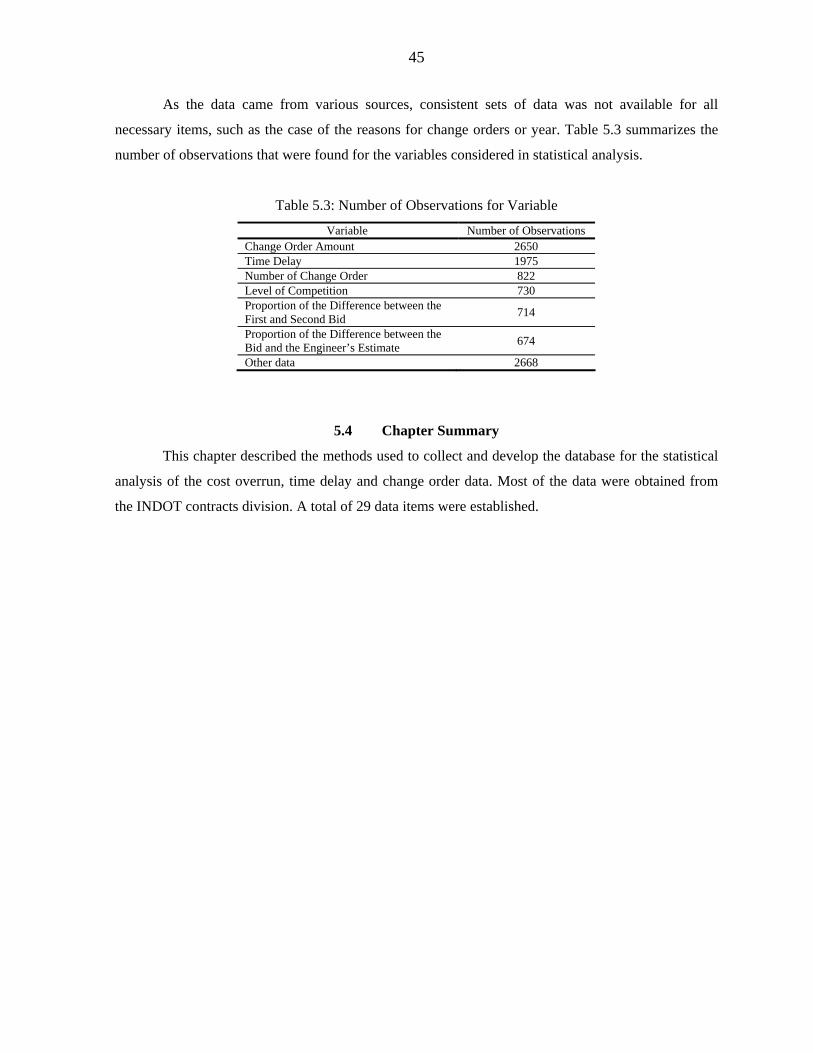
45
As the data came from various sources, consistent sets of data was not available for all
necessary items, such as the case of the reasons for change orders or year. Table 5.3 summarizes the
number of observations that were found for the variables considered in statistical analysis.
Table 5.3: Number of Observations for Variable
Variable Number of Observations Change Order Amount 2650 Time Delay 1975 Number of Change Order 822 Level of Competition 730 Proportion of the Difference between the First and Second Bid 714
Proportion of the Difference between the Bid and the Engineer’s Estimate 674
Other data 2668
5.4 Chapter Summary
This chapter described the methods used to collect and develop the database for the statistical
analysis of the cost overrun, time delay and change order data. Most of the data were obtained from
the INDOT contracts division. A total of 29 data items were established.
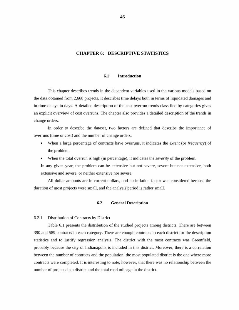
46
CHAPTER 6: DESCRIPTIVE STATISTICS
6.1 Introduction
This chapter describes trends in the dependent variables used in the various models based on
the data obtained from 2,668 projects. It describes time delays both in terms of liquidated damages and
in time delays in days. A detailed description of the cost overrun trends classified by categories gives
an explicit overview of cost overruns. The chapter also provides a detailed description of the trends in
change orders.
In order to describe the dataset, two factors are defined that describe the importance of
overruns (time or cost) and the number of change orders:
• When a large percentage of contracts have overruns, it indicates the extent (or frequency) of
the problem.
• When the total overrun is high (in percentage), it indicates the severity of the problem.
In any given year, the problem can be extensive but not severe, severe but not extensive, both
extensive and severe, or neither extensive nor severe.
All dollar amounts are in current dollars, and no inflation factor was considered because the
duration of most projects were small, and the analysis period is rather small.
6.2 General Description
6.2.1 Distribution of Contracts by District
Table 6.1 presents the distribution of the studied projects among districts. There are between
390 and 589 contracts in each category. There are enough contracts in each district for the description
statistics and to justify regression analysis. The district with the most contracts was Greenfield,
probably because the city of Indianapolis is included in this district. Moreover, there is a correlation
between the number of contracts and the population; the most populated district is the one where more
contracts were completed. It is interesting to note, however, that there was no relationship between the
number of projects in a district and the total road mileage in the district.
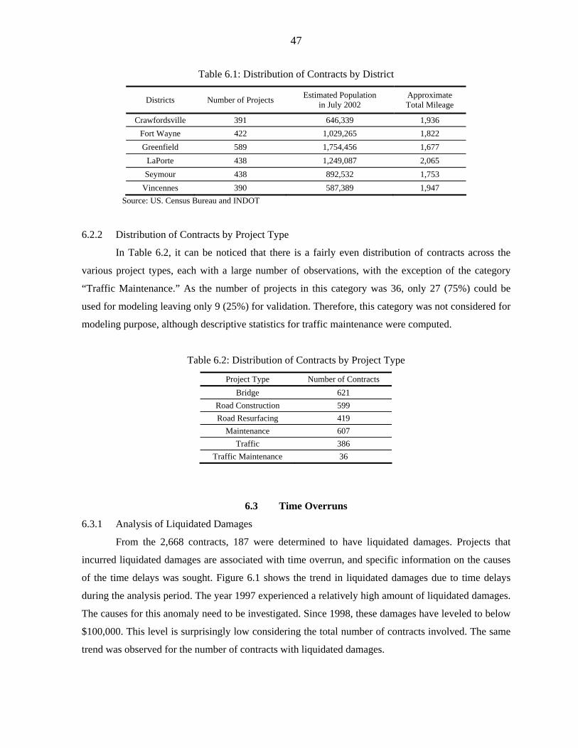
47
Table 6.1: Distribution of Contracts by District
Districts Number of Projects Estimated Population in July 2002
Approximate Total Mileage
Crawfordsville 391 646,339 1,936 Fort Wayne 422 1,029,265 1,822 Greenfield 589 1,754,456 1,677
LaPorte 438 1,249,087 2,065 Seymour 438 892,532 1,753
Vincennes 390 587,389 1,947 Source: US. Census Bureau and INDOT
6.2.2 Distribution of Contracts by Project Type
In Table 6.2, it can be noticed that there is a fairly even distribution of contracts across the
various project types, each with a large number of observations, with the exception of the category
“Traffic Maintenance.” As the number of projects in this category was 36, only 27 (75%) could be
used for modeling leaving only 9 (25%) for validation. Therefore, this category was not considered for
modeling purpose, although descriptive statistics for traffic maintenance were computed.
Table 6.2: Distribution of Contracts by Project Type
Project Type Number of Contracts Bridge 621
Road Construction 599 Road Resurfacing 419
Maintenance 607 Traffic 386
Traffic Maintenance 36
6.3 Time Overruns
6.3.1 Analysis of Liquidated Damages
From the 2,668 contracts, 187 were determined to have liquidated damages. Projects that
incurred liquidated damages are associated with time overrun, and specific information on the causes
of the time delays was sought. Figure 6.1 shows the trend in liquidated damages due to time delays
during the analysis period. The year 1997 experienced a relatively high amount of liquidated damages.
The causes for this anomaly need to be investigated. Since 1998, these damages have leveled to below
$100,000. This level is surprisingly low considering the total number of contracts involved. The same
trend was observed for the number of contracts with liquidated damages.
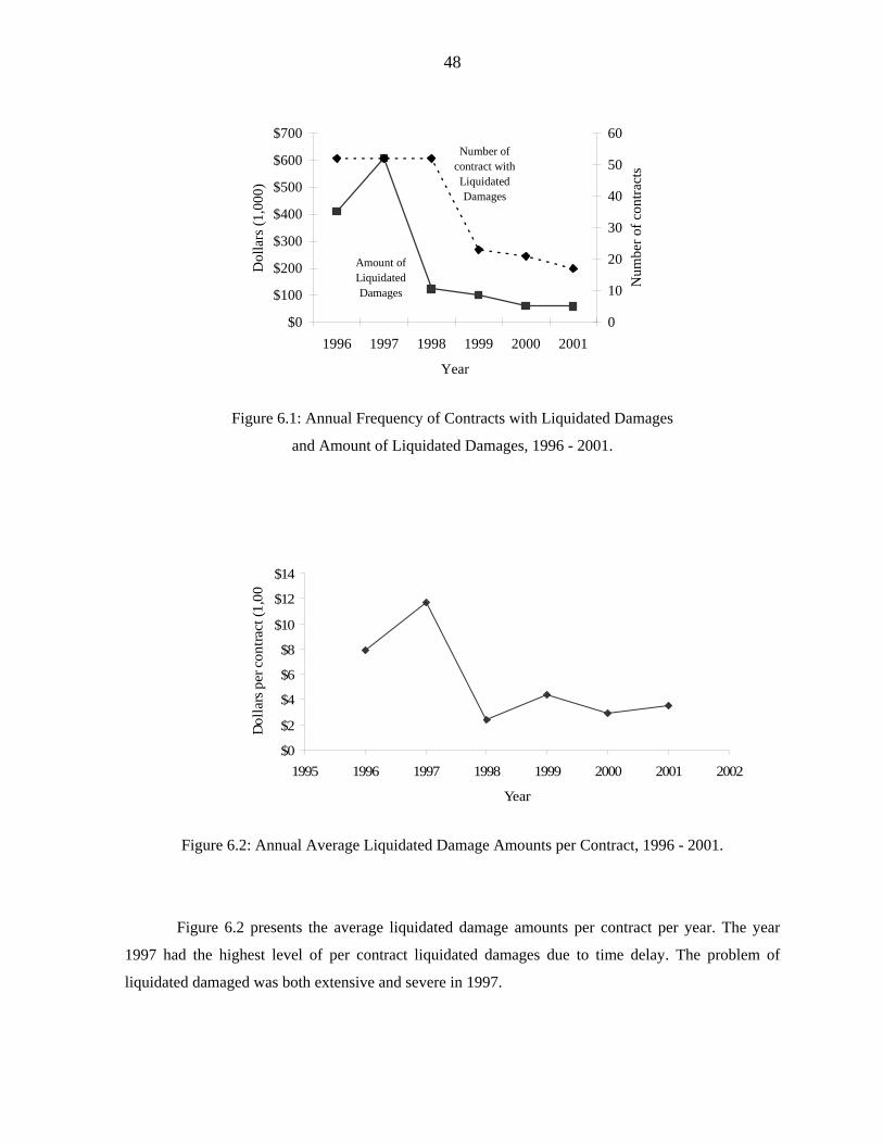
48
Amount of Liquidated Damages
Number of contract with Liquidated Damages
$0
$100
$200
$300
$400
$500
$600
$700
1996 1997 1998 1999 2000 2001
Year
Dol
lars
(1,0
00)
0
10
20
30
40
50
60
Num
ber o
f con
tract
s
Figure 6.1: Annual Frequency of Contracts with Liquidated Damages
and Amount of Liquidated Damages, 1996 - 2001.
$0
$2
$4
$6
$8
$10
$12
$14
1995 1996 1997 1998 1999 2000 2001 2002
Year
Dol
lars
per
con
tract
(1,0
0
Figure 6.2: Annual Average Liquidated Damage Amounts per Contract, 1996 - 2001.
Figure 6.2 presents the average liquidated damage amounts per contract per year. The year
1997 had the highest level of per contract liquidated damages due to time delay. The problem of
liquidated damaged was both extensive and severe in 1997.
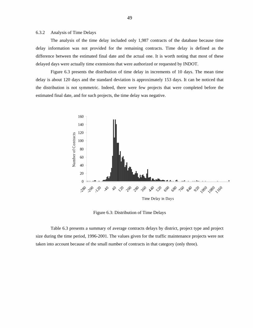
49
6.3.2 Analysis of Time Delays
The analysis of the time delay included only 1,987 contracts of the database because time
delay information was not provided for the remaining contracts. Time delay is defined as the
difference between the estimated final date and the actual one. It is worth noting that most of these
delayed days were actually time extensions that were authorized or requested by INDOT.
Figure 6.3 presents the distribution of time delay in increments of 10 days. The mean time
delay is about 120 days and the standard deviation is approximately 153 days. It can be noticed that
the distribution is not symmetric. Indeed, there were few projects that were completed before the
estimated final date, and for such projects, the time delay was negative.
0
20
40
60
80
100
120
140
160
-280 -200 -120 -40 40120 200 280 360 440 520 600 680 760 840 920
1000
1080
1160
Time Delay in Days
Num
ber o
f Con
tract
s
Figure 6.3: Distribution of Time Delays
Table 6.3 presents a summary of average contracts delays by district, project type and project
size during the time period, 1996-2001. The values given for the traffic maintenance projects were not
taken into account because of the small number of contracts in that category (only three).
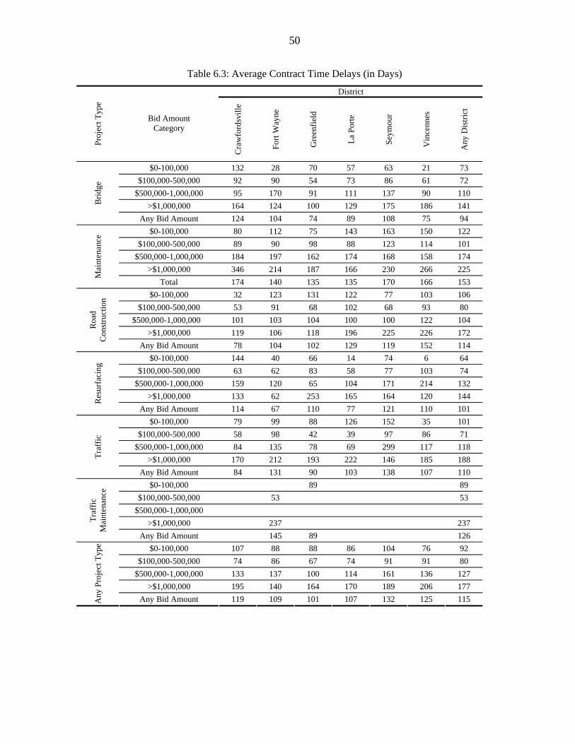
50
Table 6.3: Average Contract Time Delays (in Days)
District Pr
ojec
t Typ
e
Bid Amount Category
Cra
wfo
rdsv
ille
Fort
Way
ne
Gre
enfie
ld
La P
orte
Seym
our
Vin
cenn
es
Any
Dis
trict
$0-100,000 132 28 70 57 63 21 73 $100,000-500,000 92 90 54 73 86 61 72
$500,000-1,000,000 95 170 91 111 137 90 110 >$1,000,000 164 124 100 129 175 186 141 B
ridge
Any Bid Amount 124 104 74 89 108 75 94 $0-100,000 80 112 75 143 163 150 122
$100,000-500,000 89 90 98 88 123 114 101 $500,000-1,000,000 184 197 162 174 168 158 174
>$1,000,000 346 214 187 166 230 266 225
Mai
nten
ance
Total 174 140 135 135 170 166 153 $0-100,000 32 123 131 122 77 103 106
$100,000-500,000 53 91 68 102 68 93 80 $500,000-1,000,000 101 103 104 100 100 122 104
>$1,000,000 119 106 118 196 225 226 172
Roa
d C
onst
ruct
ion
Any Bid Amount 78 104 102 129 119 152 114 $0-100,000 144 40 66 14 74 6 64
$100,000-500,000 63 62 83 58 77 103 74 $500,000-1,000,000 159 120 65 104 171 214 132
>$1,000,000 133 62 253 165 164 120 144 Res
urfa
cing
Any Bid Amount 114 67 110 77 121 110 101 $0-100,000 79 99 88 126 152 35 101
$100,000-500,000 58 98 42 39 97 86 71 $500,000-1,000,000 84 135 78 69 299 117 118
>$1,000,000 170 212 193 222 146 185 188 Traf
fic
Any Bid Amount 84 131 90 103 138 107 110 $0-100,000 89 89
$100,000-500,000 53 53 $500,000-1,000,000
>$1,000,000 237 237 Traf
fic
Mai
nten
ance
Any Bid Amount 145 89 126 $0-100,000 107 88 88 86 104 76 92
$100,000-500,000 74 86 67 74 91 91 80 $500,000-1,000,000 133 137 100 114 161 136 127
>$1,000,000 195 140 164 170 189 206 177
Any
Pro
ject
Typ
e
Any Bid Amount 119 109 101 107 132 125 115
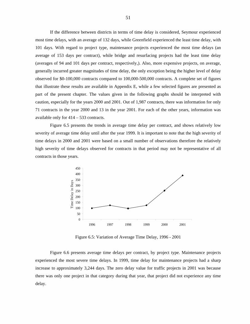
51
If the difference between districts in terms of time delay is considered, Seymour experienced
most time delays, with an average of 132 days, while Greenfield experienced the least time delay, with
101 days. With regard to project type, maintenance projects experienced the most time delays (an
average of 153 days per contract), while bridge and resurfacing projects had the least time delay
(averages of 94 and 101 days per contract, respectively,). Also, more expensive projects, on average,
generally incurred greater magnitudes of time delay, the only exception being the higher level of delay
observed for $0-100,000 contracts compared to 100,000-500,000 contracts. A complete set of figures
that illustrate these results are available in Appendix E, while a few selected figures are presented as
part of the present chapter. The values given in the following graphs should be interpreted with
caution, especially for the years 2000 and 2001. Out of 1,987 contracts, there was information for only
71 contracts in the year 2000 and 13 in the year 2001. For each of the other years, information was
available only for 414 – 533 contracts.
Figure 6.5 presents the trends in average time delay per contract, and shows relatively low
severity of average time delay until after the year 1999. It is important to note that the high severity of
time delays in 2000 and 2001 were based on a small number of observations therefore the relatively
high severity of time delays observed for contracts in that period may not be representative of all
contracts in those years.
050
100150200
250300350
400450
1996 1997 1998 1999 2000 2001
Tim
e D
elay
in D
ays
Figure 6.5: Variation of Average Time Delay, 1996 - 2001
Figure 6.6 presents average time delays per contract, by project type. Maintenance projects
experienced the most severe time delays. In 1999, time delay for maintenance projects had a sharp
increase to approximately 3,244 days. The zero delay value for traffic projects in 2001 was because
there was only one project in that category during that year, that project did not experience any time
delay.
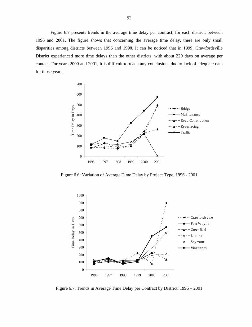
52
Figure 6.7 presents trends in the average time delay per contract, for each district, between
1996 and 2001. The figure shows that concerning the average time delay, there are only small
disparities among districts between 1996 and 1998. It can be noticed that in 1999, Crawfordsville
District experienced more time delays than the other districts, with about 220 days on average per
contact. For years 2000 and 2001, it is difficult to reach any conclusions due to lack of adequate data
for those years.
0
100
200
300
400
500
600
700
1996 1997 1998 1999 2000 2001
Tim
e D
elay
in D
ays
BridgeMaintenanceRoad ConstructionResurfacingTraffic
Figure 6.6: Variation of Average Time Delay by Project Type, 1996 - 2001
0
100
200
300
400
500
600
700
800
900
1000
1996 1997 1998 1999 2000 2001
Tim
e D
elay
in D
ays Crawfordsville
Fort WayneGreenfieldLaporteSeymourVincennes
Figure 6.7: Trends in Average Time Delay per Contract by District, 1996 – 2001
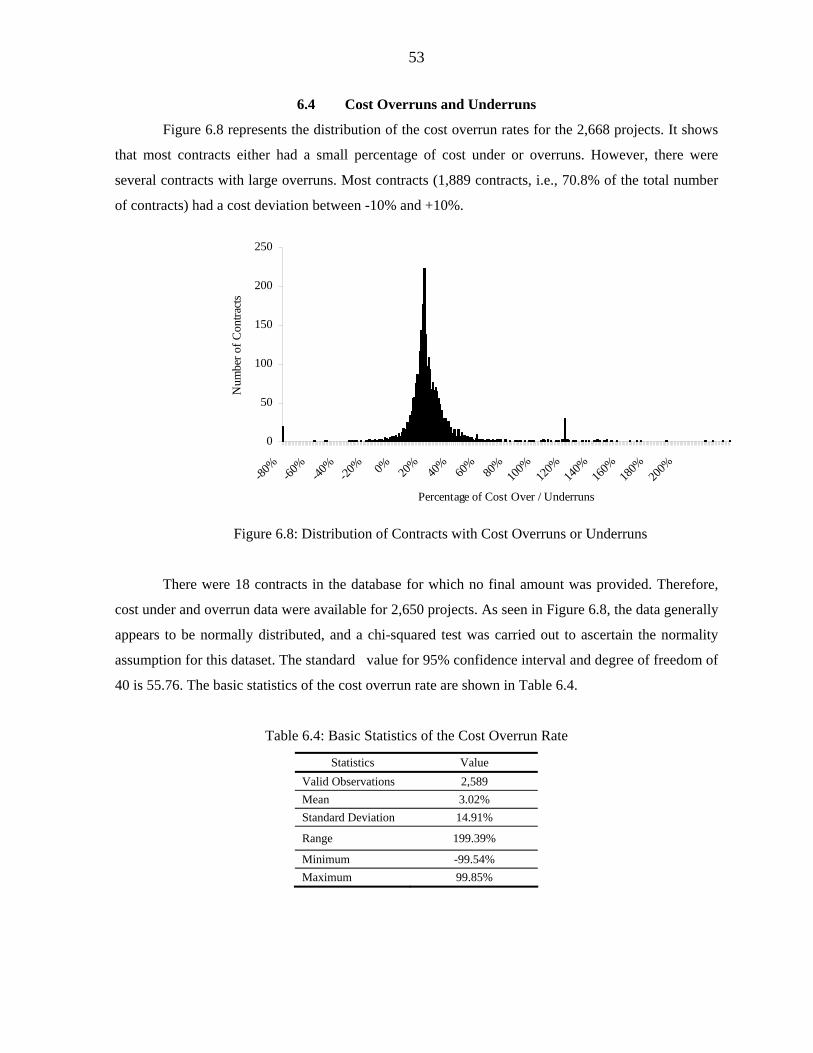
53
6.4 Cost Overruns and Underruns
Figure 6.8 represents the distribution of the cost overrun rates for the 2,668 projects. It shows
that most contracts either had a small percentage of cost under or overruns. However, there were
several contracts with large overruns. Most contracts (1,889 contracts, i.e., 70.8% of the total number
of contracts) had a cost deviation between -10% and +10%.
0
50
100
150
200
250
-80%
-60%
-40%
-20% 0% 20
%40
%60
%80
%10
0%12
0%14
0%16
0%18
0%20
0%
Percentage of Cost Over / Underruns
Num
ber o
f Con
tract
s
Figure 6.8: Distribution of Contracts with Cost Overruns or Underruns
There were 18 contracts in the database for which no final amount was provided. Therefore,
cost under and overrun data were available for 2,650 projects. As seen in Figure 6.8, the data generally
appears to be normally distributed, and a chi-squared test was carried out to ascertain the normality
assumption for this dataset. The standard value for 95% confidence interval and degree of freedom of
40 is 55.76. The basic statistics of the cost overrun rate are shown in Table 6.4.
Table 6.4: Basic Statistics of the Cost Overrun Rate
Statistics Value Valid Observations 2,589 Mean 3.02% Standard Deviation 14.91%
Range 199.39%
Minimum -99.54% Maximum 99.85%
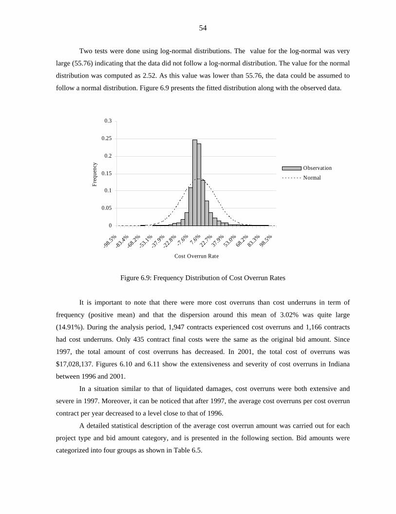
54
Two tests were done using log-normal distributions. The value for the log-normal was very
large (55.76) indicating that the data did not follow a log-normal distribution. The value for the normal
distribution was computed as 2.52. As this value was lower than 55.76, the data could be assumed to
follow a normal distribution. Figure 6.9 presents the fitted distribution along with the observed data.
0
0.05
0.1
0.15
0.2
0.25
0.3
-98.5%-83.4%
-68.2%-53.1%
-37.9%-22.8%
-7.6%7.6%
22.7%37.9%
53.0%68.2%
83.3%98.5%
Cost Overrun Rate
Freq
uenc
y
Observation
Normal
Figure 6.9: Frequency Distribution of Cost Overrun Rates
It is important to note that there were more cost overruns than cost underruns in term of
frequency (positive mean) and that the dispersion around this mean of 3.02% was quite large
(14.91%). During the analysis period, 1,947 contracts experienced cost overruns and 1,166 contracts
had cost underruns. Only 435 contract final costs were the same as the original bid amount. Since
1997, the total amount of cost overruns has decreased. In 2001, the total cost of overruns was
$17,028,137. Figures 6.10 and 6.11 show the extensiveness and severity of cost overruns in Indiana
between 1996 and 2001.
In a situation similar to that of liquidated damages, cost overruns were both extensive and
severe in 1997. Moreover, it can be noticed that after 1997, the average cost overruns per cost overrun
contract per year decreased to a level close to that of 1996.
A detailed statistical description of the average cost overrun amount was carried out for each
project type and bid amount category, and is presented in the following section. Bid amounts were
categorized into four groups as shown in Table 6.5.
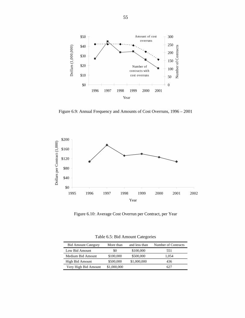
55
Amount of cost overruns
Number of cont racts with cost overruns
$0
$10
$20
$30
$40
$50
1996 1997 1998 1999 2000 2001
Year
Dol
lars
(1,0
00,0
00)
0
50
100
150
200
250
300
Num
ber o
f Con
tract
s
Figure 6.9: Annual Frequency and Amounts of Cost Overruns, 1996 – 2001
$0
$40
$80
$120
$160
$200
1995 1996 1997 1998 1999 2000 2001 2002
Year
Dol
lars
per
Con
tract
(1,0
00)
Figure 6.10: Average Cost Overrun per Contract, per Year
Table 6.5: Bid Amount Categories
Bid Amount Category More than and less than Number of Contracts Low Bid Amount $0 $100,000 551 Medium Bid Amount $100,000 $500,000 1,054 High Bid Amount $500,000 $1,000,000 436 Very High Bid Amount $1,000,000 627
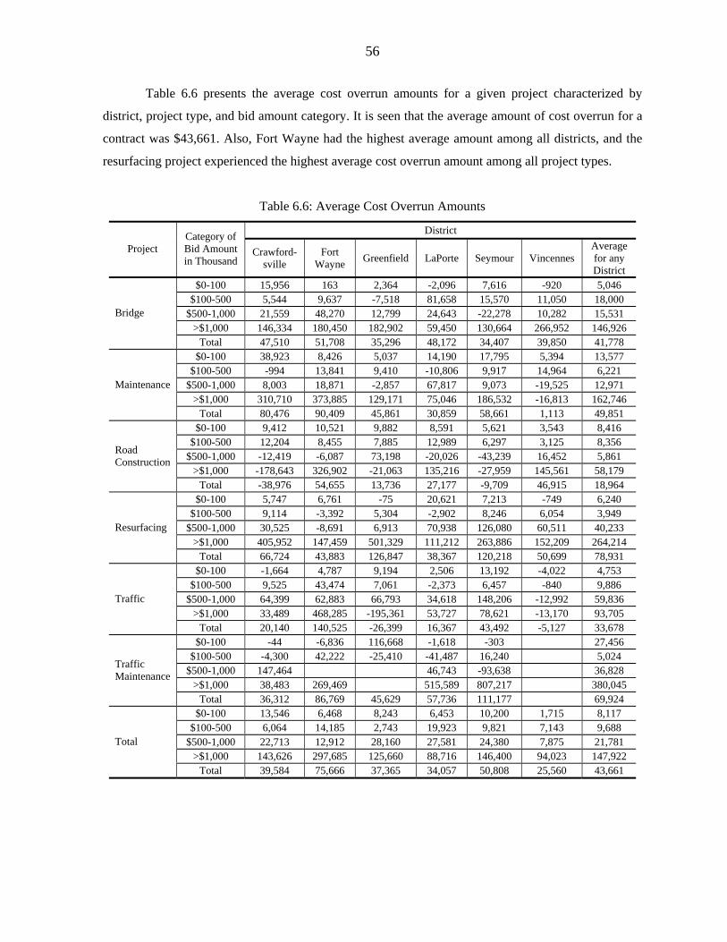
56
Table 6.6 presents the average cost overrun amounts for a given project characterized by
district, project type, and bid amount category. It is seen that the average amount of cost overrun for a
contract was $43,661. Also, Fort Wayne had the highest average amount among all districts, and the
resurfacing project experienced the highest average cost overrun amount among all project types.
Table 6.6: Average Cost Overrun Amounts
District
Project Category of Bid Amount in Thousand
Crawford- sville
Fort Wayne Greenfield LaPorte Seymour Vincennes
Average for any District
$0-100 15,956 163 2,364 -2,096 7,616 -920 5,046 $100-500 5,544 9,637 -7,518 81,658 15,570 11,050 18,000
$500-1,000 21,559 48,270 12,799 24,643 -22,278 10,282 15,531 >$1,000 146,334 180,450 182,902 59,450 130,664 266,952 146,926
Bridge
Total 47,510 51,708 35,296 48,172 34,407 39,850 41,778 $0-100 38,923 8,426 5,037 14,190 17,795 5,394 13,577
$100-500 -994 13,841 9,410 -10,806 9,917 14,964 6,221 $500-1,000 8,003 18,871 -2,857 67,817 9,073 -19,525 12,971
>$1,000 310,710 373,885 129,171 75,046 186,532 -16,813 162,746 Maintenance
Total 80,476 90,409 45,861 30,859 58,661 1,113 49,851 $0-100 9,412 10,521 9,882 8,591 5,621 3,543 8,416
$100-500 12,204 8,455 7,885 12,989 6,297 3,125 8,356 $500-1,000 -12,419 -6,087 73,198 -20,026 -43,239 16,452 5,861
>$1,000 -178,643 326,902 -21,063 135,216 -27,959 145,561 58,179
Road Construction
Total -38,976 54,655 13,736 27,177 -9,709 46,915 18,964 $0-100 5,747 6,761 -75 20,621 7,213 -749 6,240
$100-500 9,114 -3,392 5,304 -2,902 8,246 6,054 3,949 $500-1,000 30,525 -8,691 6,913 70,938 126,080 60,511 40,233
>$1,000 405,952 147,459 501,329 111,212 263,886 152,209 264,214 Resurfacing
Total 66,724 43,883 126,847 38,367 120,218 50,699 78,931 $0-100 -1,664 4,787 9,194 2,506 13,192 -4,022 4,753
$100-500 9,525 43,474 7,061 -2,373 6,457 -840 9,886 $500-1,000 64,399 62,883 66,793 34,618 148,206 -12,992 59,836
>$1,000 33,489 468,285 -195,361 53,727 78,621 -13,170 93,705 Traffic
Total 20,140 140,525 -26,399 16,367 43,492 -5,127 33,678 $0-100 -44 -6,836 116,668 -1,618 -303 27,456
$100-500 -4,300 42,222 -25,410 -41,487 16,240 5,024 $500-1,000 147,464 46,743 -93,638 36,828
>$1,000 38,483 269,469 515,589 807,217 380,045
Traffic Maintenance
Total 36,312 86,769 45,629 57,736 111,177 69,924 $0-100 13,546 6,468 8,243 6,453 10,200 1,715 8,117
$100-500 6,064 14,185 2,743 19,923 9,821 7,143 9,688 $500-1,000 22,713 12,912 28,160 27,581 24,380 7,875 21,781
>$1,000 143,626 297,685 125,660 88,716 146,400 94,023 147,922 Total
Total 39,584 75,666 37,365 34,057 50,808 25,560 43,661
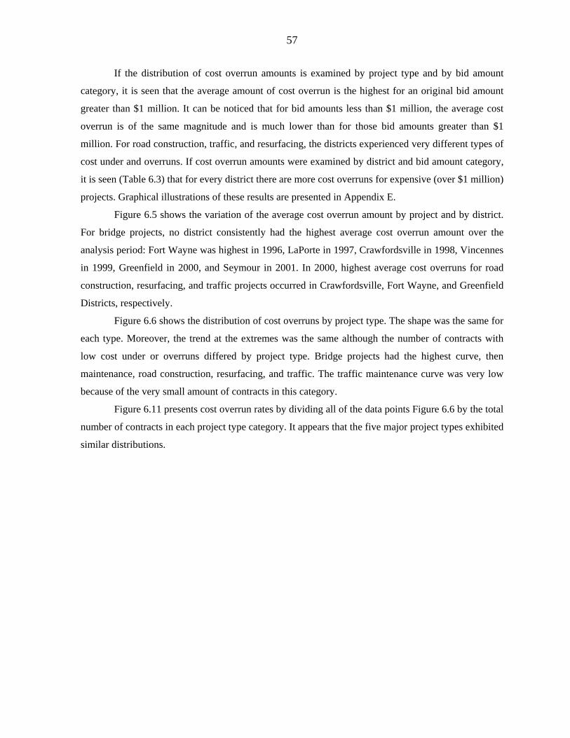
57
If the distribution of cost overrun amounts is examined by project type and by bid amount
category, it is seen that the average amount of cost overrun is the highest for an original bid amount
greater than $1 million. It can be noticed that for bid amounts less than $1 million, the average cost
overrun is of the same magnitude and is much lower than for those bid amounts greater than $1
million. For road construction, traffic, and resurfacing, the districts experienced very different types of
cost under and overruns. If cost overrun amounts were examined by district and bid amount category,
it is seen (Table 6.3) that for every district there are more cost overruns for expensive (over $1 million)
projects. Graphical illustrations of these results are presented in Appendix E.
Figure 6.5 shows the variation of the average cost overrun amount by project and by district.
For bridge projects, no district consistently had the highest average cost overrun amount over the
analysis period: Fort Wayne was highest in 1996, LaPorte in 1997, Crawfordsville in 1998, Vincennes
in 1999, Greenfield in 2000, and Seymour in 2001. In 2000, highest average cost overruns for road
construction, resurfacing, and traffic projects occurred in Crawfordsville, Fort Wayne, and Greenfield
Districts, respectively.
Figure 6.6 shows the distribution of cost overruns by project type. The shape was the same for
each type. Moreover, the trend at the extremes was the same although the number of contracts with
low cost under or overruns differed by project type. Bridge projects had the highest curve, then
maintenance, road construction, resurfacing, and traffic. The traffic maintenance curve was very low
because of the very small amount of contracts in this category.
Figure 6.11 presents cost overrun rates by dividing all of the data points Figure 6.6 by the total
number of contracts in each project type category. It appears that the five major project types exhibited
similar distributions.
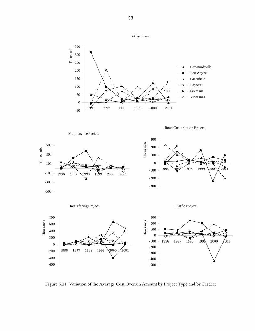
58
Bridge Project
-50
0
50
100
150
200
250
300
350
1996 1997 1998 1999 2000 2001
Thou
sand
sCrawfordsville
FortWayne
Greenfield
Laporte
Seymour
Vincennes
M aintenance Project
-500
-300
-100
100
300
500
1996 1997 1998 1999 2000 2001
Thou
sand
s
Road Construction Project
-300
-200
-100
0
100
200
300
1996 1997 1998 1999 2000 2001
Thou
sand
s
Resurfacing Project
-600
-400
-200
0
200
400
600
800
1996 1997 1998 1999 2000 2001
Thou
sand
s
T raffic Project
-500-400-300-200-100
0100200300
1996 1997 1998 1999 2000 2001
Thou
sand
s
Figure 6.11: Variation of the Average Cost Overrun Amount by Project Type and by District
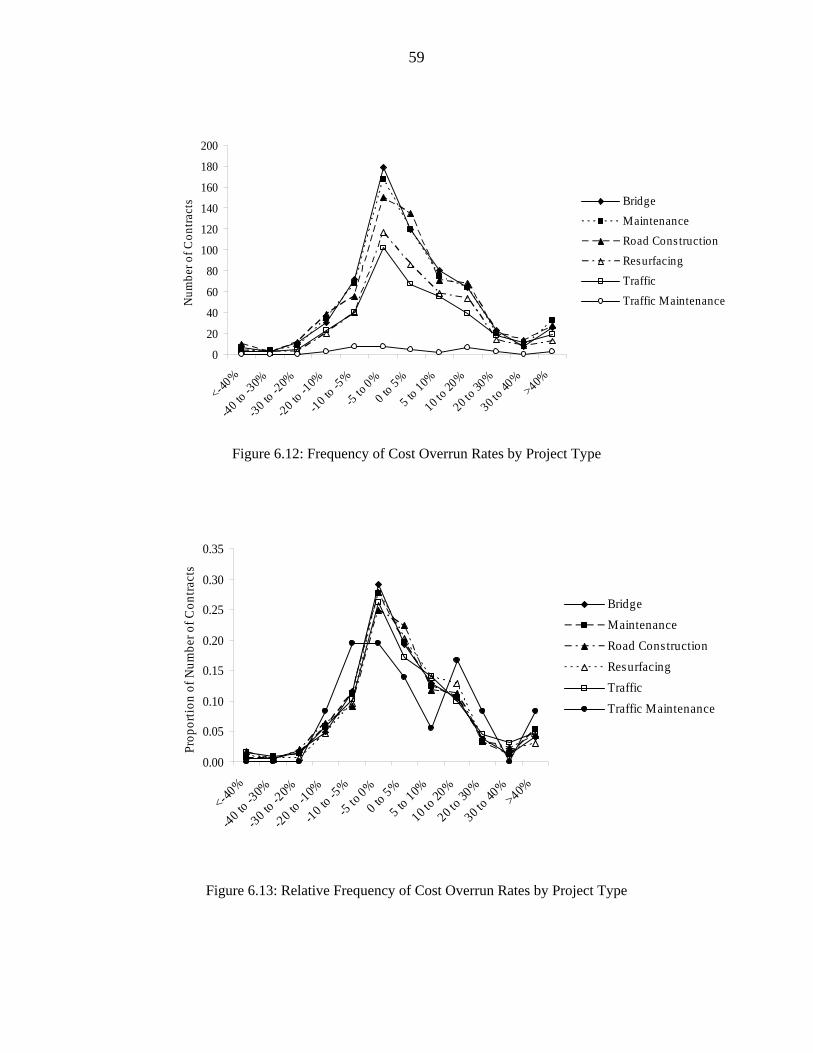
59
0
20
40
60
80
100
120
140
160
180
200
<-40%
-40 to -3
0%
-30 to -2
0%
-20 to -1
0%
-10 to -5
%
-5 to 0%
0 to 5%
5 to 10%
10 to 2
0%
20 to 3
0%
30 to 4
0%>40%
Num
ber o
f Con
tract
s BridgeMaintenanceRoad ConstructionResurfacingTrafficTraffic Maintenance
Figure 6.12: Frequency of Cost Overrun Rates by Project Type
0.00
0.05
0.10
0.15
0.20
0.25
0.30
0.35
<-40%
-40 to -3
0%
-30 to -2
0%
-20 to -1
0%
-10 to -5
%
-5 to 0%
0 to 5%
5 to 10%
10 to 2
0%
20 to 3
0%
30 to 4
0%>40%
Prop
ortio
n of
Num
ber o
f Con
tract
s
BridgeMaintenanceRoad ConstructionResurfacingTrafficTraffic Maintenance
Figure 6.13: Relative Frequency of Cost Overrun Rates by Project Type
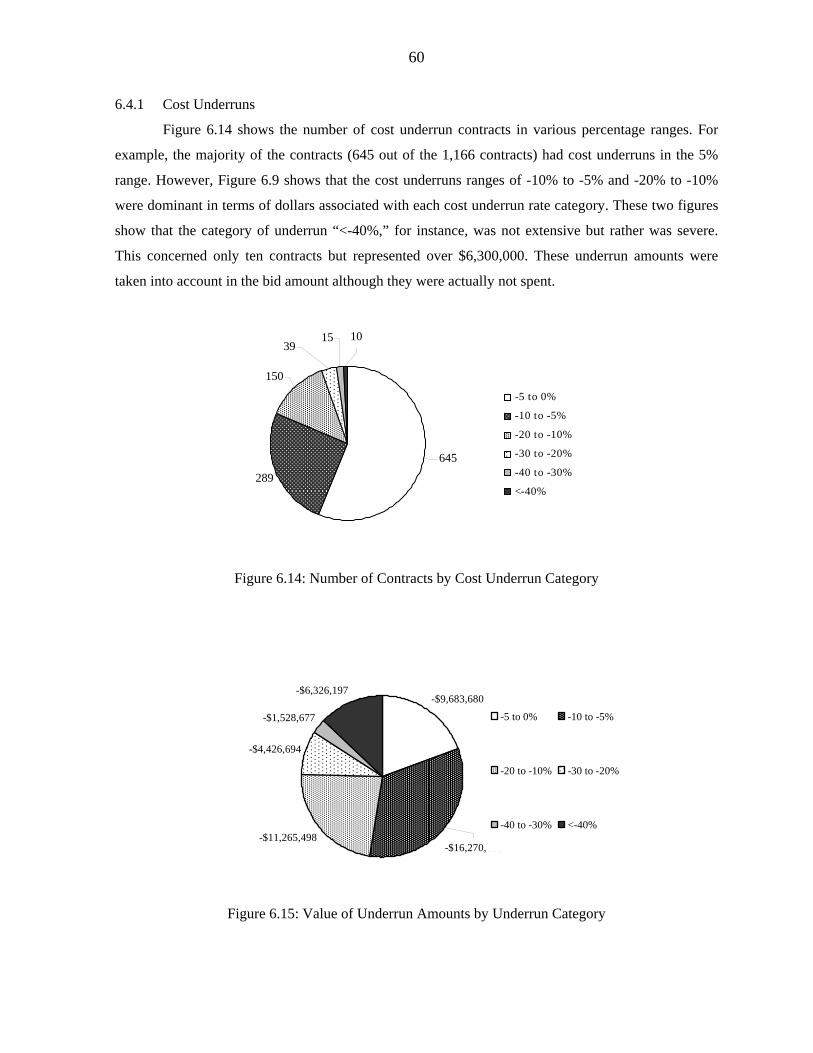
60
6.4.1 Cost Underruns
Figure 6.14 shows the number of cost underrun contracts in various percentage ranges. For
example, the majority of the contracts (645 out of the 1,166 contracts) had cost underruns in the 5%
range. However, Figure 6.9 shows that the cost underruns ranges of -10% to -5% and -20% to -10%
were dominant in terms of dollars associated with each cost underrun rate category. These two figures
show that the category of underrun “<-40%,” for instance, was not extensive but rather was severe.
This concerned only ten contracts but represented over $6,300,000. These underrun amounts were
taken into account in the bid amount although they were actually not spent.
645
289
150
3915 10
-5 to 0%
-10 to -5%
-20 to -10%
-30 to -20%
-40 to -30%
<-40%
Figure 6.14: Number of Contracts by Cost Underrun Category
-$9,683,680
-$11,265,498
-$4,426,694
-$1,528,677
-$6,326,197
-$16,270,105
-5 to 0% -10 to -5%
-20 to -10% -30 to -20%
-40 to -30% <-40%
Figure 6.15: Value of Underrun Amounts by Underrun Category
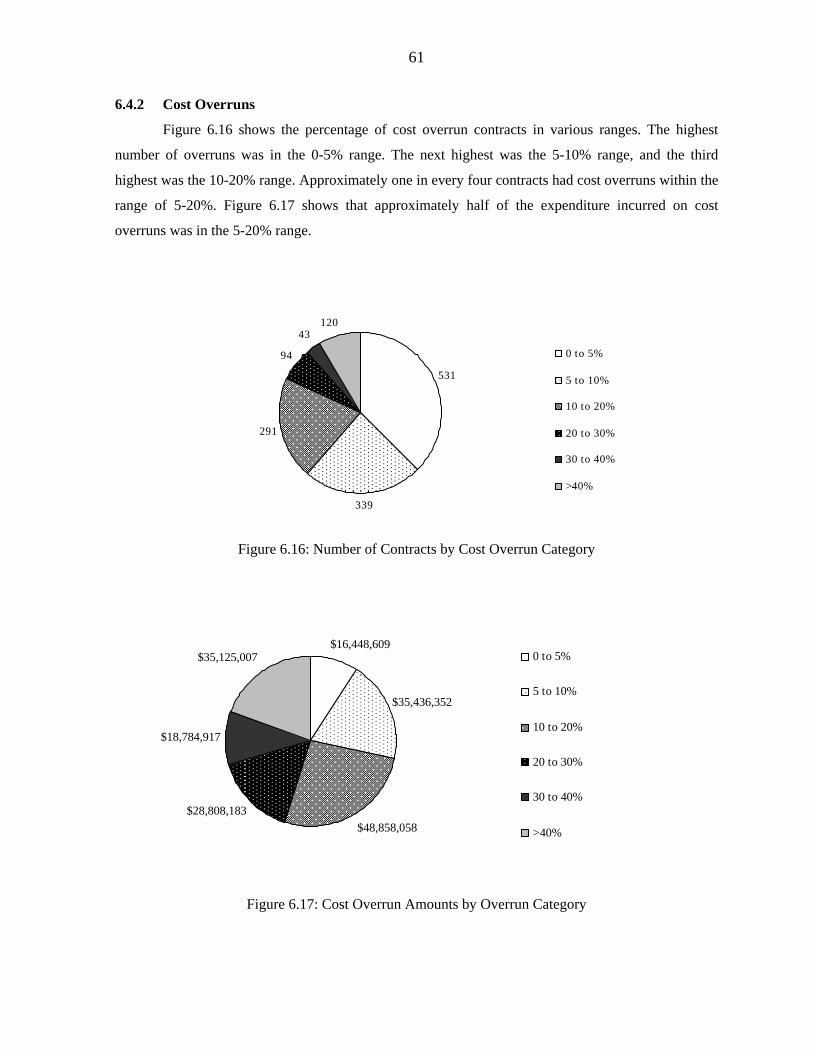
61
6.4.2 Cost Overruns
Figure 6.16 shows the percentage of cost overrun contracts in various ranges. The highest
number of overruns was in the 0-5% range. The next highest was the 5-10% range, and the third
highest was the 10-20% range. Approximately one in every four contracts had cost overruns within the
range of 5-20%. Figure 6.17 shows that approximately half of the expenditure incurred on cost
overruns was in the 5-20% range.
291
339
531
120 43
94 0 to 5%
5 to 10%
10 to 20%
20 to 30%
30 to 40%
>40%
Figure 6.16: Number of Contracts by Cost Overrun Category
$16,448,609
$35,436,352
$48,858,058$28,808,183
$18,784,917
$35,125,007 0 to 5%
5 to 10%
10 to 20%
20 to 30%
30 to 40%
>40%
Figure 6.17: Cost Overrun Amounts by Overrun Category
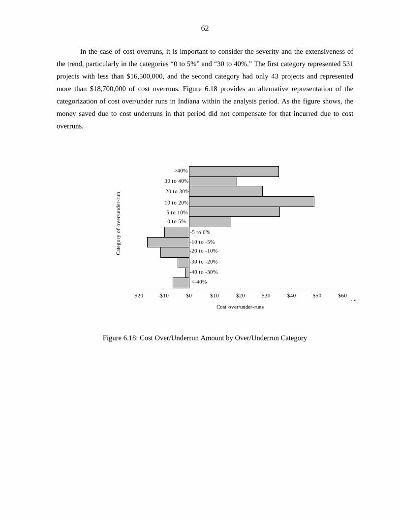
62
In the case of cost overruns, it is important to consider the severity and the extensiveness of
the trend, particularly in the categories “0 to 5%” and “30 to 40%.” The first category represented 531
projects with less than $16,500,000, and the second category had only 43 projects and represented
more than $18,700,000 of cost overruns. Figure 6.18 provides an alternative representation of the
categorization of cost over/under runs in Indiana within the analysis period. As the figure shows, the
money saved due to cost underruns in that period did not compensate for that incurred due to cost
overruns.
<-40%
-40 to -30%
-30 to -20%
-20 to -10%-10 to -5%
-5 to 0%
0 to 5%5 to 10%
10 to 20%
20 to 30%
30 to 40%
>40%
-$20 -$10 $0 $10 $20 $30 $40 $50 $60 lion
Cate
gory
of o
ver/u
nder
-run
Cost over/under-runs
Figure 6.18: Cost Over/Underrun Amount by Over/Underrun Category
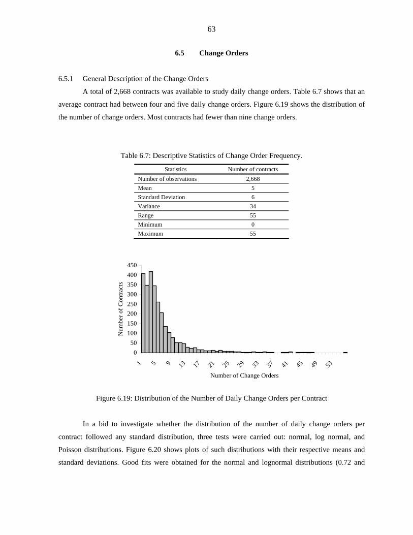
63
6.5 Change Orders
6.5.1 General Description of the Change Orders
A total of 2,668 contracts was available to study daily change orders. Table 6.7 shows that an
average contract had between four and five daily change orders. Figure 6.19 shows the distribution of
the number of change orders. Most contracts had fewer than nine change orders.
Table 6.7: Descriptive Statistics of Change Order Frequency.
Statistics Number of contracts Number of observations 2,668 Mean 5 Standard Deviation 6 Variance 34 Range 55 Minimum 0 Maximum 55
050
100150200250300350400450
1 5 9 13 17 21 25 29 33 37 41 45 49 53
Number of Change Orders
Num
ber o
f Con
tract
s
Figure 6.19: Distribution of the Number of Daily Change Orders per Contract
In a bid to investigate whether the distribution of the number of daily change orders per
contract followed any standard distribution, three tests were carried out: normal, log normal, and
Poisson distributions. Figure 6.20 shows plots of such distributions with their respective means and
standard deviations. Good fits were obtained for the normal and lognormal distributions (0.72 and
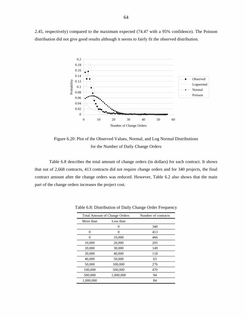
64
2.45, respectively) compared to the maximum expected (74.47 with a 95% confidence). The Poisson
distribution did not give good results although it seems to fairly fit the observed distribution.
00.020.040.060.08
0.10.120.140.160.18
0.2
0 10 20 30 40 50 60
Number of Change Orders
Prob
abili
ty ObservedLognormalNormalPoisson
Figure 6.20: Plot of the Observed Values, Normal, and Log Normal Distributions
for the Number of Daily Change Orders
Table 6.8 describes the total amount of change orders (in dollars) for each contract. It shows
that out of 2,668 contracts, 413 contracts did not require change orders and for 340 projects, the final
contract amount after the change orders was reduced. However, Table 6.2 also shows that the main
part of the change orders increases the project cost.
Table 6.8: Distribution of Daily Change Order Frequency
Total Amount of Change Orders Number of contracts More than Less than
0 340 0 0 413 0 10,000 466
10,000 20,000 205 20,000 30,000 149 30,000 40,000 118 40,000 50,000 63 50,000 100,000 276 100,000 500,000 470 500,000 1,000,000 94
1,000,000 84
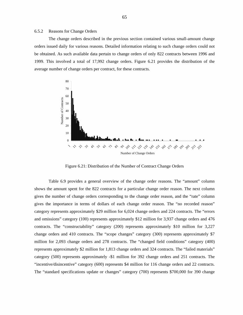
65
6.5.2 Reasons for Change Orders
The change orders described in the previous section contained various small-amount change
orders issued daily for various reasons. Detailed information relating to such change orders could not
be obtained. As such available data pertain to change orders of only 822 contracts between 1996 and
1999. This involved a total of 17,992 change orders. Figure 6.21 provides the distribution of the
average number of change orders per contract, for these contracts.
0
10
20
30
40
50
60
70
80
1 11 21 31 41 51 61 71 81 91 101
111
121
131
141
151
161
171
181
191
201
211
221
Number of Change Orders
Num
ber o
f Con
tract
s
Figure 6.21: Distribution of the Number of Contract Change Orders
Table 6.9 provides a general overview of the change order reasons. The “amount” column
shows the amount spent for the 822 contracts for a particular change order reason. The next column
gives the number of change orders corresponding to the change order reason, and the “rate” column
gives the importance in terms of dollars of each change order reason. The “no recorded reason”
category represents approximately $29 million for 6,024 change orders and 224 contracts. The “errors
and omissions” category (100) represents approximately $12 million for 3,937 change orders and 476
contracts. The “constructability” category (200) represents approximately $10 million for 3,227
change orders and 410 contracts. The “scope changes” category (300) represents approximately $7
million for 2,093 change orders and 278 contracts. The “changed field conditions” category (400)
represents approximately $2 million for 1,813 change orders and 324 contracts. The “failed materials”
category (500) represents approximately -$1 million for 392 change orders and 251 contracts. The
“incentive/disincentive” category (600) represents $4 million for 116 change orders and 22 contracts.
The “standard specifications update or changes” category (700) represents $700,000 for 390 change
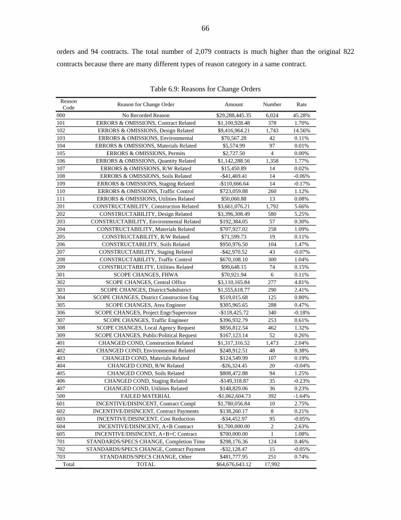
66
orders and 94 contracts. The total number of 2,079 contracts is much higher than the original 822
contracts because there are many different types of reason category in a same contract.
Table 6.9: Reasons for Change Orders Reason Code Reason for Change Order Amount Number Rate
000 No Recorded Reason $29,288,445.35 6,024 45.28% 101 ERRORS & OMISSIONS, Contract Related $1,100,928.48 378 1.70% 102 ERRORS & OMISSIONS, Design Related $9,416,964.21 1,743 14.56% 103 ERRORS & OMISSIONS, Environmental $70,567.28 42 0.11% 104 ERRORS & OMISSIONS, Materials Related $5,574.99 97 0.01% 105 ERRORS & OMISSIONS, Permits $2,727.50 4 0.00% 106 ERRORS & OMISSIONS, Quantity Related $1,142,288.56 1,358 1.77% 107 ERRORS & OMISSIONS, R/W Related $15,450.89 14 0.02% 108 ERRORS & OMISSIONS, Soils Related -$41,469.41 14 -0.06% 109 ERRORS & OMISSIONS, Staging Related -$110,666.64 14 -0.17% 110 ERRORS & OMISSIONS, Traffic Control $723,059.88 260 1.12% 111 ERRORS & OMISSIONS, Utilities Related $50,060.88 13 0.08% 201 CONSTRUCTABILITY, Construction Related $3,661,076.21 1,792 5.66% 202 CONSTRUCTABILITY, Design Related $3,396,308.49 580 5.25% 203 CONSTRUCTABILITY, Environmental Related $192,384.05 57 0.30% 204 CONSTRUCTABILITY, Materials Related $707,927.02 258 1.09% 205 CONSTRUCTABILITY, R/W Related $71,599.73 19 0.11% 206 CONSTRUCTABILITY, Soils Related $950,976.50 104 1.47% 207 CONSTRUCTABILITY, Staging Related -$42,970.52 43 -0.07% 208 CONSTRUCTABILITY, Traffic Control $670,108.10 300 1.04% 209 CONSTRUCTABILITY, Utilities Related $99,648.15 74 0.15% 301 SCOPE CHANGES, FHWA $70,921.94 6 0.11% 302 SCOPE CHANGES, Central Office $3,110,165.84 277 4.81% 303 SCOPE CHANGES, District/Subdistrict $1,555,618.77 290 2.41% 304 SCOPE CHANGES, District Construction Eng $519,015.68 125 0.80% 305 SCOPE CHANGES, Area Engineer $305,965.65 288 0.47% 306 SCOPE CHANGES, Project Engr/Supervisor -$118,425.72 340 -0.18% 307 SCOPE CHANGES, Traffic Engineer $396,932.79 253 0.61% 308 SCOPE CHANGES, Local Agency Request $856,812.54 462 1.32% 309 SCOPE CHANGES, Public/Political Request $167,123.14 52 0.26% 401 CHANGED COND, Construction Related $1,317,316.52 1,473 2.04% 402 CHANGED COND, Environmental Related $248,912.51 48 0.38% 403 CHANGED COND, Materials Related $124,549.99 107 0.19% 404 CHANGED COND, R/W Related -$26,324.45 20 -0.04% 405 CHANGED COND, Soils Related $808,472.88 94 1.25% 406 CHANGED COND, Staging Related -$149,318.87 35 -0.23% 407 CHANGED COND, Utilities Related $148,829.06 36 0.23% 500 FAILED MATERIAL -$1,062,604.73 392 -1.64% 601 INCENTIVE/DISINCENT, Contract Compl $1,780,056.84 10 2.75% 602 INCENTIVE/DISINCENT, Contract Payments $138,260.17 8 0.21% 603 INCENTIVE/DISINCENT, Cost Reduction -$34,452.97 95 -0.05% 604 INCENTIVE/DISINCENT, A+B Contract $1,700,000.00 2 2.63% 605 INCENTIVE/DISINCENT, A+B+C Contract $700,000.00 1 1.08% 701 STANDARDS/SPECS CHANGE, Completion Time $298,176.36 124 0.46% 702 STANDARDS/SPECS CHANGE, Contract Payment -$32,128.47 15 -0.05% 703 STANDARDS/SPECS CHANGE, Other $481,777.95 251 0.74%
Total TOTAL $64,676,643.12 17,992
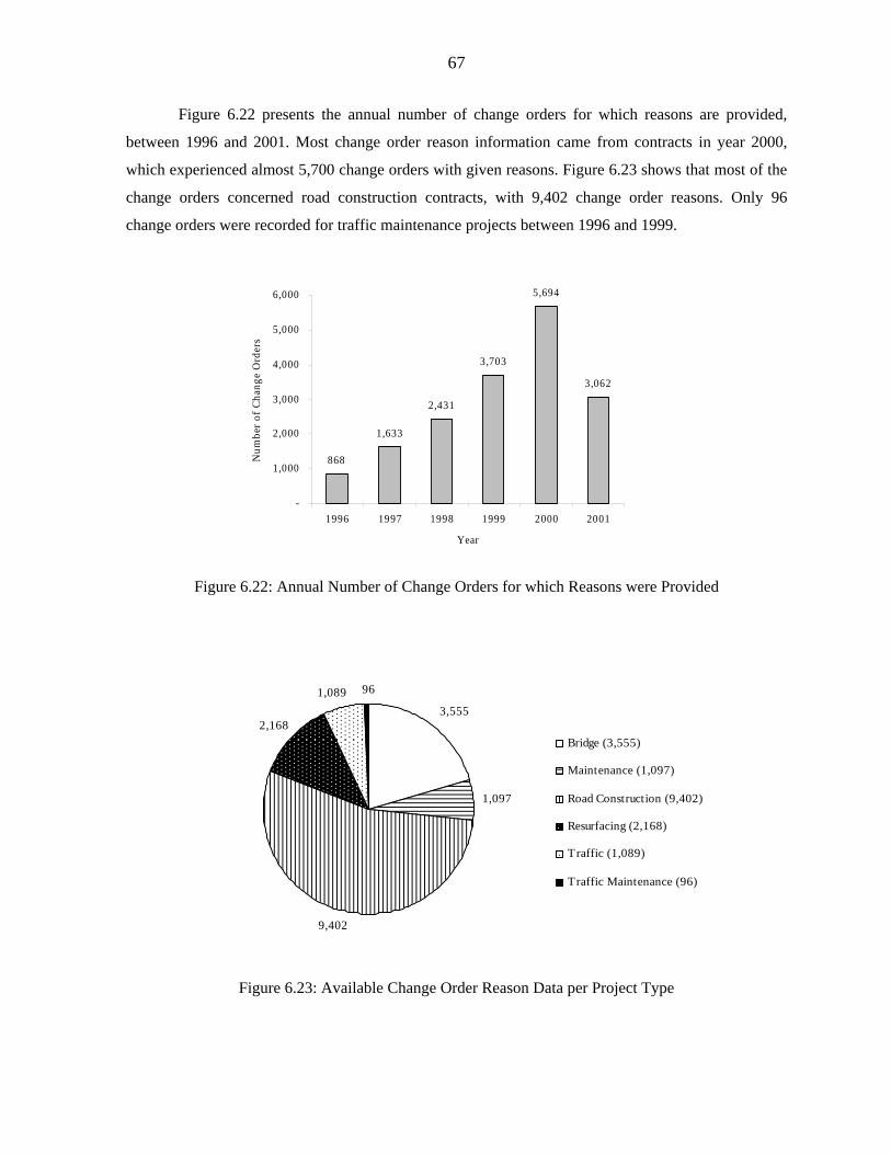
67
Figure 6.22 presents the annual number of change orders for which reasons are provided,
between 1996 and 2001. Most change order reason information came from contracts in year 2000,
which experienced almost 5,700 change orders with given reasons. Figure 6.23 shows that most of the
change orders concerned road construction contracts, with 9,402 change order reasons. Only 96
change orders were recorded for traffic maintenance projects between 1996 and 1999.
868
1,633
2,431
3,703
5,694
3,062
-
1,000
2,000
3,000
4,000
5,000
6,000
1996 1997 1998 1999 2000 2001
Year
Num
ber o
f Cha
nge
Ord
ers
Figure 6.22: Annual Number of Change Orders for which Reasons were Provided
3,555
1,097
9,402
2,168
1,089 96
Bridge (3,555)
Maintenance (1,097)
Road Construction (9,402)
Resurfacing (2,168)
Traffic (1,089)
Traffic Maintenance (96)
Figure 6.23: Available Change Order Reason Data per Project Type
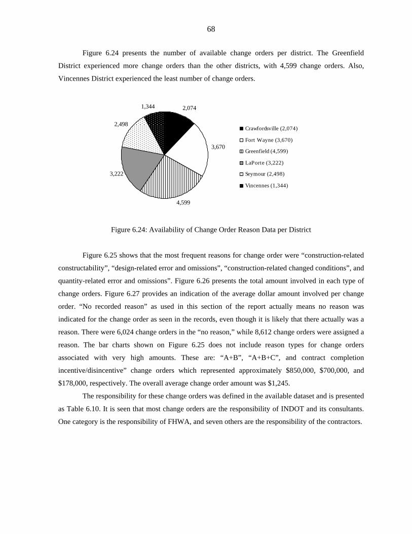
68
Figure 6.24 presents the number of available change orders per district. The Greenfield
District experienced more change orders than the other districts, with 4,599 change orders. Also,
Vincennes District experienced the least number of change orders.
2,074
3,670
4,599
3,222
2,498
1,344
Crawfordsville (2,074)
Fort Wayne (3,670)
Greenfield (4,599)
LaPorte (3,222)
Seymour (2,498)
Vincennes (1,344)
Figure 6.24: Availability of Change Order Reason Data per District
Figure 6.25 shows that the most frequent reasons for change order were “construction-related
constructability”, “design-related error and omissions”, “construction-related changed conditions”, and
quantity-related error and omissions”. Figure 6.26 presents the total amount involved in each type of
change orders. Figure 6.27 provides an indication of the average dollar amount involved per change
order. “No recorded reason” as used in this section of the report actually means no reason was
indicated for the change order as seen in the records, even though it is likely that there actually was a
reason. There were 6,024 change orders in the “no reason,” while 8,612 change orders were assigned a
reason. The bar charts shown on Figure 6.25 does not include reason types for change orders
associated with very high amounts. These are: “A+B”, “A+B+C”, and contract completion
incentive/disincentive” change orders which represented approximately $850,000, $700,000, and
$178,000, respectively. The overall average change order amount was $1,245.
The responsibility for these change orders was defined in the available dataset and is presented
as Table 6.10. It is seen that most change orders are the responsibility of INDOT and its consultants.
One category is the responsibility of FHWA, and seven others are the responsibility of the contractors.
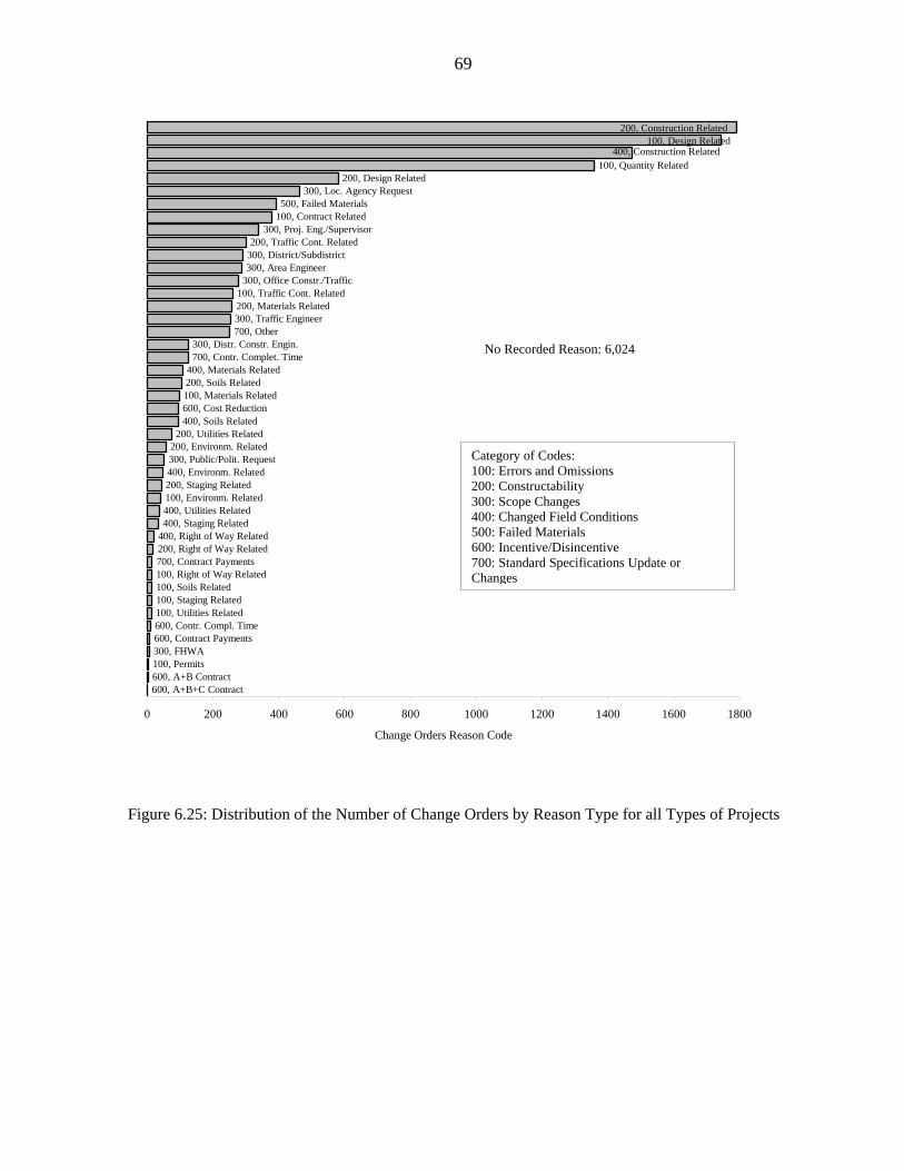
69
600, A+B+C Contract600, A+B Contract100, Permits300, FHWA600, Contract Payments600, Contr. Compl. Time100, Utilities Related100, Staging Related100, Soils Related100, Right of Way Related700, Contract Payments200, Right of Way Related400, Right of Way Related400, Staging Related400, Utilities Related100, Environm. Related200, Staging Related400, Environm. Related300, Public/Polit. Request200, Environm. Related
200, Utilities Related400, Soils Related600, Cost Reduction100, Materials Related200, Soils Related400, Materials Related
700, Contr. Complet. Time300, Distr. Constr. Engin.
700, Other300, Traffic Engineer200, Materials Related100, Traffic Cont. Related
300, Office Constr./Traffic300, Area Engineer300, District/Subdistrict200, Traffic Cont. Related
300, Proj. Eng./Supervisor100, Contract Related
300, Loc. Agency Request200, Design Related
100, Quantity Related
500, Failed Materials
200, Construction Related100, Design Related
400, Construction Related
0 200 400 600 800 1000 1200 1400 1600 1800
Change Orders Reason Code
Figure 6.25: Distribution of the Number of Change Orders by Reason Type for all Types of Projects
Category of Codes: 100: Errors and Omissions 200: Constructability 300: Scope Changes 400: Changed Field Conditions 500: Failed Materials 600: Incentive/Disincentive 700: Standard Specifications Update or Changes
No Recorded Reason: 6,024
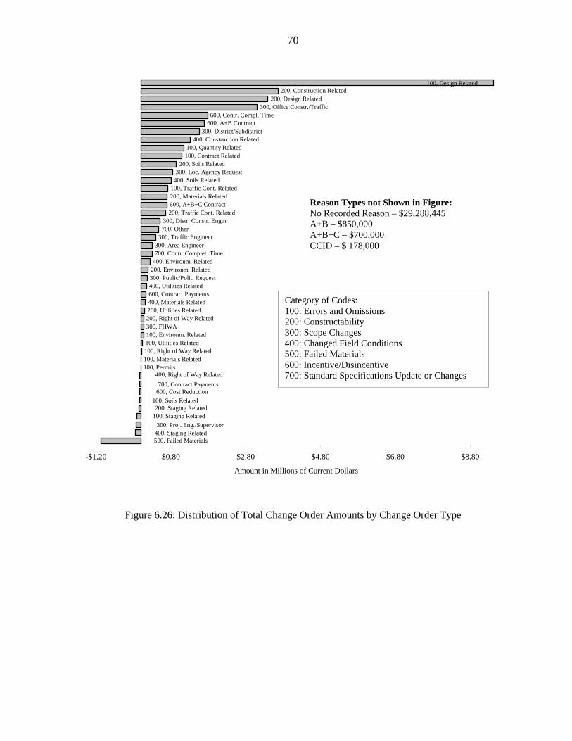
70
100, Permits100, Materials Related100, Right of Way Related100, Utilities Related100, Environm. Related300, FHWA200, Right of Way Related200, Utilities Related400, Materials Related600, Contract Payments400, Utilities Related300, Public/Polit. Request200, Environm. Related400, Environm. Related700, Contr. Complet. Time300, Area Engineer
300, Traffic Engineer700, Other300, Distr. Constr. Engin.
200, Traffic Cont. Related600, A+B+C Contract200, Materials Related100, Traffic Cont. Related
400, Soils Related300, Loc. Agency Request
200, Soils Related100, Contract Related100, Quantity Related
400, Construction Related300, District/Subdistrict
600, A+B Contract600, Contr. Compl. Time
300, Office Constr./Traffic200, Design Related
200, Construction Related100, Design Related
700, Contract Payments600, Cost Reduction
100, Soils Related200, Staging Related
100, Staging Related300, Proj. Eng./Supervisor
400, Staging Related500, Failed Materials
400, Right of Way Related
-$1.20 $0.80 $2.80 $4.80 $6.80 $8.80
Amount in Millions of Current Dollars
Figure 6.26: Distribution of Total Change Order Amounts by Change Order Type
Category of Codes: 100: Errors and Omissions 200: Constructability 300: Scope Changes 400: Changed Field Conditions 500: Failed Materials 600: Incentive/Disincentive 700: Standard Specifications Update or Changes
Reason Types not Shown in Figure: No Recorded Reason – $29,288,445 A+B – $850,000 A+B+C – $700,000 CCID – $ 178,000
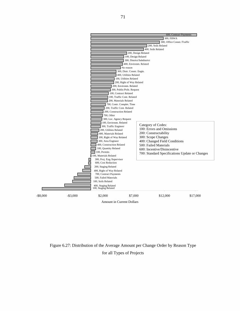
71
100, Materials Related100, Permits100, Quantity Related400, Construction Related300, Area Engineer100, Right of Way Related400, Materials Related200, Utilities Related
300, Traffic Engineer100, Environm. Related300, Loc. Agency Request700, Other200, Construction Related200, Traffic Cont. Related700, Contr. Complet. Time
200, Materials Related100, Traffic Cont. Related100, Contract Related
300, Public/Polit. Request200, Environm. Related
200, Right of Way Related100, Utilities Related
400, Utilities Related300, Distr. Constr. Engin.
No reason400, Environm. Related300, District/Subdistrict100, Design Related
200, Design Related400, Soils Related
200, Soils Related300, Office Constr./Traffic
300, FHWA
300, Proj. Eng./Supervisor
100, Staging Related400, Staging Related100, Soils Related
500, Failed Materials700, Contract Payments
400, Right of Way Related200, Staging Related600, Cost Reduction
600, Contract Payments
-$8,000 -$3,000 $2,000 $7,000 $12,000 $17,000
Amount in Current Dollars
Figure 6.27: Distribution of the Average Amount per Change Order by Reason Type
for all Types of Projects
Category of Codes: 100: Errors and Omissions 200: Constructability 300: Scope Changes 400: Changed Field Conditions 500: Failed Materials 600: Incentive/Disincentive 700: Standard Specifications Update or Changes
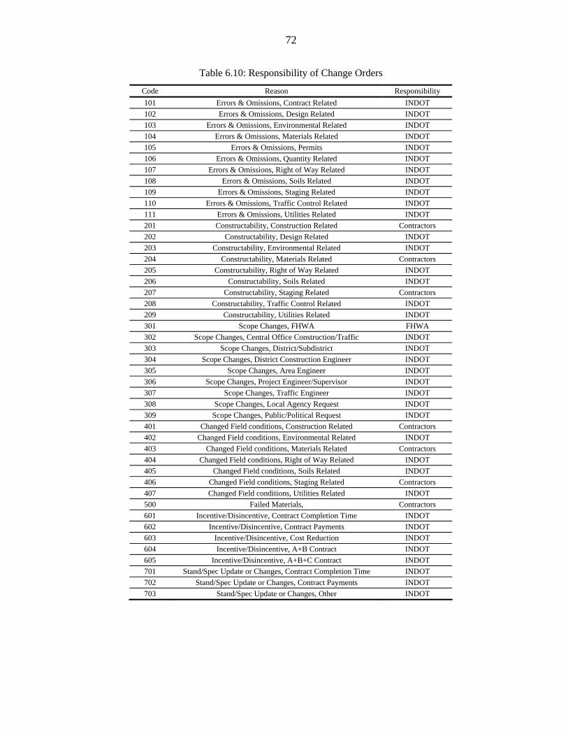
72
Table 6.10: Responsibility of Change Orders
Code Reason Responsibility 101 Errors & Omissions, Contract Related INDOT 102 Errors & Omissions, Design Related INDOT 103 Errors & Omissions, Environmental Related INDOT 104 Errors & Omissions, Materials Related INDOT 105 Errors & Omissions, Permits INDOT 106 Errors & Omissions, Quantity Related INDOT 107 Errors & Omissions, Right of Way Related INDOT 108 Errors & Omissions, Soils Related INDOT 109 Errors & Omissions, Staging Related INDOT 110 Errors & Omissions, Traffic Control Related INDOT 111 Errors & Omissions, Utilities Related INDOT 201 Constructability, Construction Related Contractors 202 Constructability, Design Related INDOT 203 Constructability, Environmental Related INDOT 204 Constructability, Materials Related Contractors 205 Constructability, Right of Way Related INDOT 206 Constructability, Soils Related INDOT 207 Constructability, Staging Related Contractors 208 Constructability, Traffic Control Related INDOT 209 Constructability, Utilities Related INDOT 301 Scope Changes, FHWA FHWA 302 Scope Changes, Central Office Construction/Traffic INDOT 303 Scope Changes, District/Subdistrict INDOT 304 Scope Changes, District Construction Engineer INDOT 305 Scope Changes, Area Engineer INDOT 306 Scope Changes, Project Engineer/Supervisor INDOT 307 Scope Changes, Traffic Engineer INDOT 308 Scope Changes, Local Agency Request INDOT 309 Scope Changes, Public/Political Request INDOT 401 Changed Field conditions, Construction Related Contractors 402 Changed Field conditions, Environmental Related INDOT 403 Changed Field conditions, Materials Related Contractors 404 Changed Field conditions, Right of Way Related INDOT 405 Changed Field conditions, Soils Related INDOT 406 Changed Field conditions, Staging Related Contractors 407 Changed Field conditions, Utilities Related INDOT 500 Failed Materials, Contractors 601 Incentive/Disincentive, Contract Completion Time INDOT 602 Incentive/Disincentive, Contract Payments INDOT 603 Incentive/Disincentive, Cost Reduction INDOT 604 Incentive/Disincentive, A+B Contract INDOT 605 Incentive/Disincentive, A+B+C Contract INDOT 701 Stand/Spec Update or Changes, Contract Completion Time INDOT 702 Stand/Spec Update or Changes, Contract Payments INDOT 703 Stand/Spec Update or Changes, Other INDOT
73
The data shows that over $30 million of change orders were the responsibility of INDOT or
their consultants; approximately $70,000 was due to FHWA, and over $4.5 million was due to the
contractors. Change orders are classified as preventable or non preventable. In Indiana, there is clear
definition of what constitutes a preventable or non preventable change order [INDOT, 2002].
Preventable change orders include those due to errors and omissions in contract documents,
constructability problems, and changes in scope of the project. On the other hand, non preventable
change orders are those associated with changed field conditions, failed materials,
incentive/disincentive provisions, and changes or updates to standards/specifications. Further
explanation of each category of preventable and non preventable change orders are provided in
Appendices A and C of this report. Using these definitions, the present study determined that of the
$30 million due to INDOT or its consultants for change orders incurred on contract between 1996 and
2001, about $25 million was preventable.
For bridge projects, the reasons associated with the highest change order amount were "design
related errors and omissions", and construction related changes field conditions. Again, the "no
reason" change orders represented more than $6.5 million, which is large compared to the
approximately$10million spent overall in change orders in this category (bridge projects). More than
$2.5 million was related to change orders due to INDOT, with more than $2.3 million that could have
been prevented. FHWA was responsible for no change orders in bridge projects, less than $1 million
was due to the contractors, and more than half of it could have been prevented.
Road construction projects also experienced the highest amount of change orders in the type
“design related errors and omission." The "no reason" was approximately $19.8 million, while the
total amount of change orders for bridge projects was approximately $40 million. More than $19
million was the responsibility of INDOT, and more than $14 million could have been prevented. More
than $700,000 spent on change orders were due to the contractors and actually about $1 million were
preventable (some not preventable change orders were negative amounts).
The most important reasons for change orders in terms of amount spent in maintenance
projects were the following: "design related errors and omissions,” "construction completion time in
constructability," and "construction and environmental related changed filed conditions." In
maintenance projects, the "no reason" change orders represented more than $532,000. The percentage
of the dollar amount of "no reason" change order out of the total change order amount for maintenance
projects (22.4%) was not as high as for other project categories. For maintenance projects, about $1.5
million of the change orders out of $2.37 million was the responsibility, of INDOT, with less than
$900,000 preventable. Moreover, the contractors were responsible for more than $380,000, with half
74
of it preventable. The data on this project category did not indicate any FHW A responsibility for
change orders.
For traffic projects, the amount of money spent in change orders involved mostly traffic
related reasons ("traffic engineer" and "scope changes"). It is also interesting to notice that in this
category of projects, "construction related changes field conditions" and district construction
engineering scope changes," the change orders resulted in a smaller final amount (were negative
amounts). Approximately $680,000 was the responsibility of INDOT and most of it was preventable.
About $118,000 out of $380,000 in change orders that were the responsibility of the contractors could
have been prevented.
For resurfacing, "design related errors and omissions" and "construction related in
constructability" Were the main reasons for change order amounts. For such projects, approximately
all of $5.3 million spent on INDOT responsible change orders could have been prevented.
Approximately $1.3million was the responsibility of the contractors, but most of this amount came
from "construction related constructability: and was preventable. In this category of projects, over
$70,000 was attributed to FHWA change orders.
Among the 96 change orders recorded in the traffic maintenance projects, only 2 had a reason
for such change orders, "construction related changed filed conditions" and "district/sub district scope
changes".
Concerning the distribution of change order reasons per district location, the "errors and
omission, design related" was always at the first or second position for the most expensive reasons for
change orders, except in the Crawfordsville District where it was at the fourth position. The "error and
omission" reason category was in every district the most expensive one in terms of change order
attributable to INDOT.
Figure 6.26 shows that the most influential change order reason was “design related errors and
omissions,” with almost $10 million. It must be added that for approximately $29,300,000 (which
represents 45% of the total change orders available for the study) no explicit reason was given for the
change order. Figure 6.26 does not take into account such “no-reason” change orders. A second
category of reasons for change orders was “construction-related and design-related constructability”
and “Central Office scope changes,” with approximately $3.1 to $3.6 million. Some change order
reasons do not represent a large amount, such as, the following “errors and omissions reasons”:
“environmental-related,” “utilities-related,” “right-of-way related,” “materials-related,” and “permits
related.” On the contrary, the failed material reason for change orders generally resulted in a
diminution of the contract amount. Indeed, it is obvious that INDOT would not pay for a failed work.
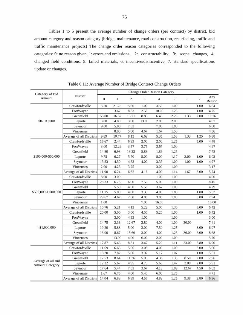
75
Tables 1 to 5 present the average number of change orders (per contract) by district, bid
amount category and reason category (bridge, maintenance, road construction, resurfacing, traffic and
traffic maintenance projects) The change order reason categories corresponded to the following
categories: 0: no reason given, 1: errors and omissions, 2: constructability, 3: scope changes, 4:
changed field conditions, 5: failed materials, 6: incentive/disincentive, 7: standard specifications
update or changes.
Table 6.11: Average Number of Bridge Contract Change Orders
Change Order Reason Category Category of Bid Amount District
0 1 2 3 4 5 6 7 Any Reason
Crawfordsville 3.50 21.25 5.60 1.00 3.50 1.00 1.00 6.64 FortWayne 3.67 8.33 2.50 10.00 1.25 1.00 4.25 Greenfield 56.00 16.57 13.71 8.83 6.40 2.25 1.33 2.00 10.26
Laporte 3.00 4.80 3.00 13.00 2.00 2.00 4.07 Seymour 9.00 5.00 7.33 7.00 1.00 6.08
Vincennes 8.00 5.00 4.67 1.67 1.50 4.36
$0-100,000
Average of all Districts 9.89 10.77 8.13 6.62 5.35 1.53 1.33 1.25 6.88 Crawfordsville 16.67 2.44 6.33 2.00 2.00 1.25 5.00 4.48
FortWayne 3.00 12.29 3.57 3.75 3.67 1.00 4.97 Greenfield 14.80 6.93 13.22 5.88 1.86 1.25 7.75
Laporte 9.75 6.27 5.70 5.00 8.00 1.17 3.00 1.00 6.02 Seymour 13.83 4.50 4.33 4.00 3.33 1.00 1.00 1.00 4.97
Vincennes 2.00 4.25 3.25 3.00 1.00 3.17
$100,000-500,000
Average of all Districts 11.90 6.24 6.62 4.16 4.00 1.14 1.67 3.00 5.74 Crawfordsville 8.00 3.00 1.00 1.00 4.00
FortWayne 28.33 6.75 6.00 7.50 5.00 1.00 8.45 Greenfield 5.50 4.50 5.50 3.67 1.00 4.29
Laporte 11.75 5.00 4.00 3.33 4.00 1.83 1.00 5.52 Seymour 29.67 4.67 2.60 4.00 3.00 1.00 5.00 7.94
Vincennes 1.00 7.00 16.00 10.00
$500,000-1,000,000
Average of all Districts 16.76 5.21 4.13 5.22 5.05 1.36 3.00 6.42 Crawfordsville 20.00 5.00 3.00 4.50 5.20 1.00 1.00 6.42
FortWayne 3.00 4.33 1.00 1.00 3.00 Greenfield 14.75 2.33 12.67 2.80 4.00 1.00 30.00 7.41
Laporte 19.20 5.88 5.00 3.00 7.50 1.25 3.00 6.97 Seymour 13.00 8.67 15.60 3.00 4.00 1.25 36.00 6.00 8.68
Vincennes 13.00 4.00 6.00 2.00 1.00 5.20
>$1,000,000
Average of all Districts 17.87 5.46 8.31 3.47 5.20 1.11 33.00 3.80 6.90 Crawfordsville 11.69 6.65 5.06 3.08 4.00 1.09 3.00 5.66
FortWayne 18.20 7.82 5.06 3.92 5.17 1.07 1.00 5.51 Greenfield 17.53 8.64 11.36 5.95 4.36 1.35 8.50 2.00 7.96
Laporte 12.32 5.67 4.95 4.73 5.60 1.47 3.00 2.00 5.91 Seymour 17.64 5.44 7.32 3.67 4.13 1.09 12.67 4.50 6.63
Vincennes 1.67 6.75 4.00 5.40 6.00 1.25 4.71
Average of all Bid Amount Category
Average of all Districts 14.04 6.88 6.99 4.56 4.82 1.25 9.38 2.80 6.36
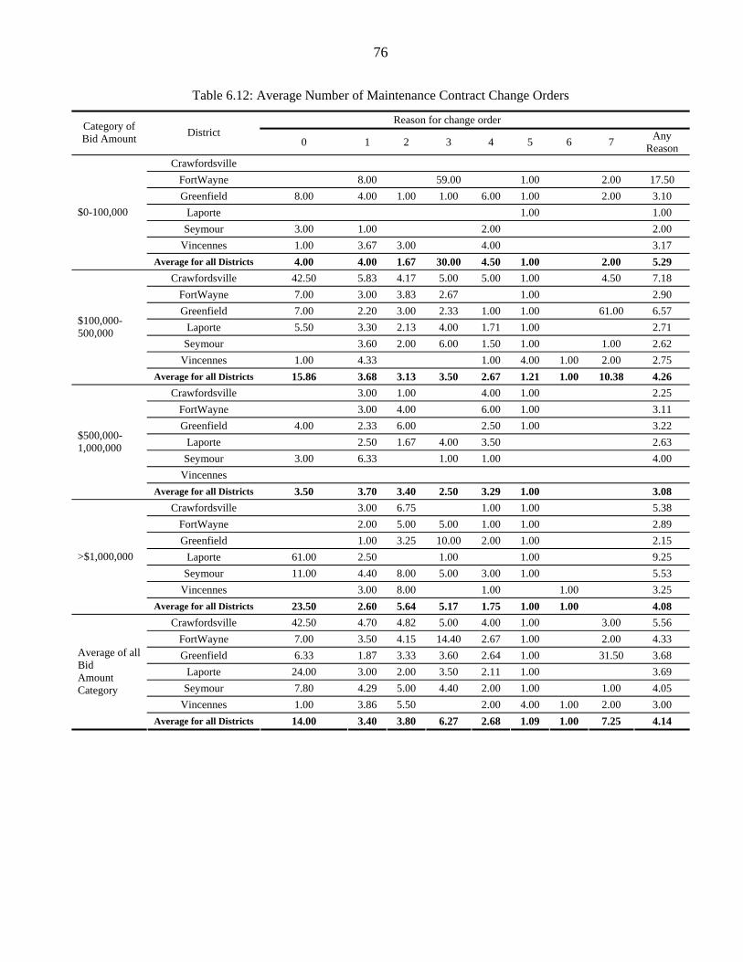
76
Table 6.12: Average Number of Maintenance Contract Change Orders
Reason for change order Category of Bid Amount District
0 1 2 3 4 5 6 7 Any Reason
Crawfordsville FortWayne 8.00 59.00 1.00 2.00 17.50 Greenfield 8.00 4.00 1.00 1.00 6.00 1.00 2.00 3.10
Laporte 1.00 1.00 Seymour 3.00 1.00 2.00 2.00
Vincennes 1.00 3.67 3.00 4.00 3.17
$0-100,000
Average for all Districts 4.00 4.00 1.67 30.00 4.50 1.00 2.00 5.29 Crawfordsville 42.50 5.83 4.17 5.00 5.00 1.00 4.50 7.18
FortWayne 7.00 3.00 3.83 2.67 1.00 2.90 Greenfield 7.00 2.20 3.00 2.33 1.00 1.00 61.00 6.57
Laporte 5.50 3.30 2.13 4.00 1.71 1.00 2.71 Seymour 3.60 2.00 6.00 1.50 1.00 1.00 2.62
Vincennes 1.00 4.33 1.00 4.00 1.00 2.00 2.75
$100,000-500,000
Average for all Districts 15.86 3.68 3.13 3.50 2.67 1.21 1.00 10.38 4.26 Crawfordsville 3.00 1.00 4.00 1.00 2.25
FortWayne 3.00 4.00 6.00 1.00 3.11 Greenfield 4.00 2.33 6.00 2.50 1.00 3.22
Laporte 2.50 1.67 4.00 3.50 2.63 Seymour 3.00 6.33 1.00 1.00 4.00
Vincennes
$500,000-1,000,000
Average for all Districts 3.50 3.70 3.40 2.50 3.29 1.00 3.08 Crawfordsville 3.00 6.75 1.00 1.00 5.38
FortWayne 2.00 5.00 5.00 1.00 1.00 2.89 Greenfield 1.00 3.25 10.00 2.00 1.00 2.15
Laporte 61.00 2.50 1.00 1.00 9.25 Seymour 11.00 4.40 8.00 5.00 3.00 1.00 5.53
Vincennes 3.00 8.00 1.00 1.00 3.25
>$1,000,000
Average for all Districts 23.50 2.60 5.64 5.17 1.75 1.00 1.00 4.08 Crawfordsville 42.50 4.70 4.82 5.00 4.00 1.00 3.00 5.56
FortWayne 7.00 3.50 4.15 14.40 2.67 1.00 2.00 4.33 Greenfield 6.33 1.87 3.33 3.60 2.64 1.00 31.50 3.68
Laporte 24.00 3.00 2.00 3.50 2.11 1.00 3.69 Seymour 7.80 4.29 5.00 4.40 2.00 1.00 1.00 4.05
Vincennes 1.00 3.86 5.50 2.00 4.00 1.00 2.00 3.00
Average of all Bid Amount Category
Average for all Districts 14.00 3.40 3.80 6.27 2.68 1.09 1.00 7.25 4.14
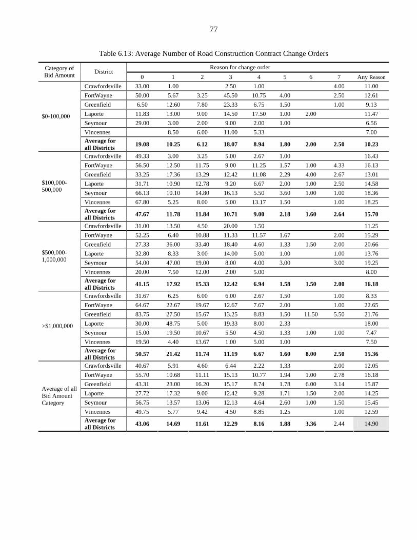
77
Table 6.13: Average Number of Road Construction Contract Change Orders
Reason for change order Category of Bid Amount District
0 1 2 3 4 5 6 7 Any Reason Crawfordsville 33.00 1.00 2.50 1.00 4.00 11.00 FortWayne 50.00 5.67 3.25 45.50 10.75 4.00 2.50 12.61 Greenfield 6.50 12.60 7.80 23.33 6.75 1.50 1.00 9.13 Laporte 11.83 13.00 9.00 14.50 17.50 1.00 2.00 11.47 Seymour 29.00 3.00 2.00 9.00 2.00 1.00 6.56 Vincennes 8.50 6.00 11.00 5.33 7.00
$0-100,000
Average for all Districts 19.08 10.25 6.12 18.07 8.94 1.80 2.00 2.50 10.23
Crawfordsville 49.33 3.00 3.25 5.00 2.67 1.00 16.43 FortWayne 56.50 12.50 11.75 9.00 11.25 1.57 1.00 4.33 16.13 Greenfield 33.25 17.36 13.29 12.42 11.08 2.29 4.00 2.67 13.01 Laporte 31.71 10.90 12.78 9.20 6.67 2.00 1.00 2.50 14.58 Seymour 66.13 10.10 14.80 16.13 5.50 3.60 1.00 1.00 18.36 Vincennes 67.80 5.25 8.00 5.00 13.17 1.50 1.00 18.25
$100,000-500,000
Average for all Districts 47.67 11.78 11.84 10.71 9.00 2.18 1.60 2.64 15.70
Crawfordsville 31.00 13.50 4.50 20.00 1.50 11.25 FortWayne 52.25 6.40 10.88 11.33 11.57 1.67 2.00 15.29 Greenfield 27.33 36.00 33.40 18.40 4.60 1.33 1.50 2.00 20.66 Laporte 32.80 8.33 3.00 14.00 5.00 1.00 1.00 13.76 Seymour 54.00 47.00 19.00 8.00 4.00 3.00 3.00 19.25 Vincennes 20.00 7.50 12.00 2.00 5.00 8.00
$500,000-1,000,000
Average for all Districts 41.15 17.92 15.33 12.42 6.94 1.58 1.50 2.00 16.18
Crawfordsville 31.67 6.25 6.00 6.00 2.67 1.50 1.00 8.33 FortWayne 64.67 22.67 19.67 12.67 7.67 2.00 1.00 22.65 Greenfield 83.75 27.50 15.67 13.25 8.83 1.50 11.50 5.50 21.76 Laporte 30.00 48.75 5.00 19.33 8.00 2.33 18.00 Seymour 15.00 19.50 10.67 5.50 4.50 1.33 1.00 1.00 7.47 Vincennes 19.50 4.40 13.67 1.00 5.00 1.00 7.50
>$1,000,000
Average for all Districts 50.57 21.42 11.74 11.19 6.67 1.60 8.00 2.50 15.36
Crawfordsville 40.67 5.91 4.60 6.44 2.22 1.33 2.00 12.05 FortWayne 55.70 10.68 11.11 15.13 10.77 1.94 1.00 2.78 16.18 Greenfield 43.31 23.00 16.20 15.17 8.74 1.78 6.00 3.14 15.87 Laporte 27.72 17.32 9.00 12.42 9.28 1.71 1.50 2.00 14.25 Seymour 56.75 13.57 13.06 12.13 4.64 2.60 1.00 1.50 15.45 Vincennes 49.75 5.77 9.42 4.50 8.85 1.25 1.00 12.59
Average of all Bid Amount Category
Average for all Districts 43.06 14.69 11.61 12.29 8.16 1.88 3.36 2.44 14.90
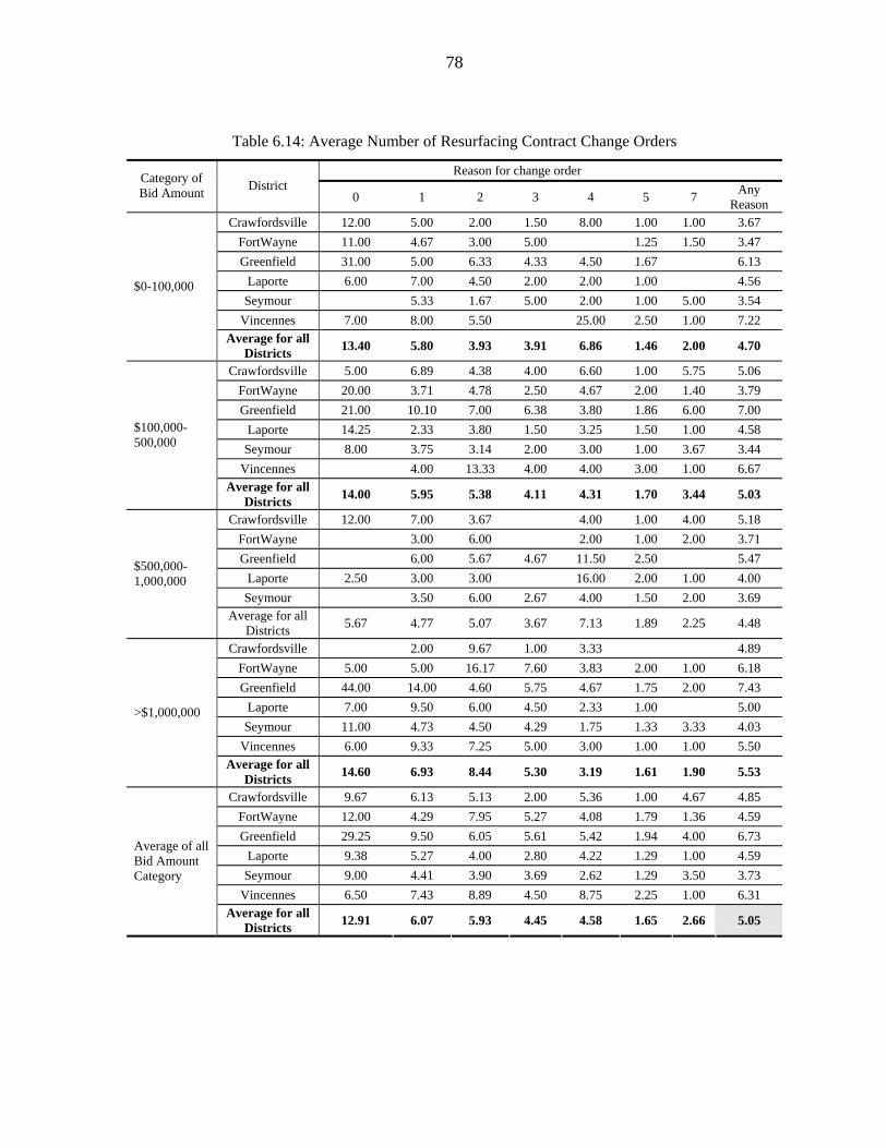
78
Table 6.14: Average Number of Resurfacing Contract Change Orders
Reason for change order Category of Bid Amount District
0 1 2 3 4 5 7 Any Reason
Crawfordsville 12.00 5.00 2.00 1.50 8.00 1.00 1.00 3.67 FortWayne 11.00 4.67 3.00 5.00 1.25 1.50 3.47 Greenfield 31.00 5.00 6.33 4.33 4.50 1.67 6.13
Laporte 6.00 7.00 4.50 2.00 2.00 1.00 4.56 Seymour 5.33 1.67 5.00 2.00 1.00 5.00 3.54
Vincennes 7.00 8.00 5.50 25.00 2.50 1.00 7.22
$0-100,000
Average for all Districts 13.40 5.80 3.93 3.91 6.86 1.46 2.00 4.70
Crawfordsville 5.00 6.89 4.38 4.00 6.60 1.00 5.75 5.06 FortWayne 20.00 3.71 4.78 2.50 4.67 2.00 1.40 3.79 Greenfield 21.00 10.10 7.00 6.38 3.80 1.86 6.00 7.00
Laporte 14.25 2.33 3.80 1.50 3.25 1.50 1.00 4.58 Seymour 8.00 3.75 3.14 2.00 3.00 1.00 3.67 3.44
Vincennes 4.00 13.33 4.00 4.00 3.00 1.00 6.67
$100,000-500,000
Average for all Districts 14.00 5.95 5.38 4.11 4.31 1.70 3.44 5.03
Crawfordsville 12.00 7.00 3.67 4.00 1.00 4.00 5.18 FortWayne 3.00 6.00 2.00 1.00 2.00 3.71 Greenfield 6.00 5.67 4.67 11.50 2.50 5.47
Laporte 2.50 3.00 3.00 16.00 2.00 1.00 4.00 Seymour 3.50 6.00 2.67 4.00 1.50 2.00 3.69
$500,000-1,000,000
Average for all Districts 5.67 4.77 5.07 3.67 7.13 1.89 2.25 4.48
Crawfordsville 2.00 9.67 1.00 3.33 4.89 FortWayne 5.00 5.00 16.17 7.60 3.83 2.00 1.00 6.18 Greenfield 44.00 14.00 4.60 5.75 4.67 1.75 2.00 7.43
Laporte 7.00 9.50 6.00 4.50 2.33 1.00 5.00 Seymour 11.00 4.73 4.50 4.29 1.75 1.33 3.33 4.03
Vincennes 6.00 9.33 7.25 5.00 3.00 1.00 1.00 5.50
>$1,000,000
Average for all Districts 14.60 6.93 8.44 5.30 3.19 1.61 1.90 5.53
Crawfordsville 9.67 6.13 5.13 2.00 5.36 1.00 4.67 4.85 FortWayne 12.00 4.29 7.95 5.27 4.08 1.79 1.36 4.59 Greenfield 29.25 9.50 6.05 5.61 5.42 1.94 4.00 6.73
Laporte 9.38 5.27 4.00 2.80 4.22 1.29 1.00 4.59 Seymour 9.00 4.41 3.90 3.69 2.62 1.29 3.50 3.73
Vincennes 6.50 7.43 8.89 4.50 8.75 2.25 1.00 6.31
Average of all Bid Amount Category
Average for all Districts 12.91 6.07 5.93 4.45 4.58 1.65 2.66 5.05
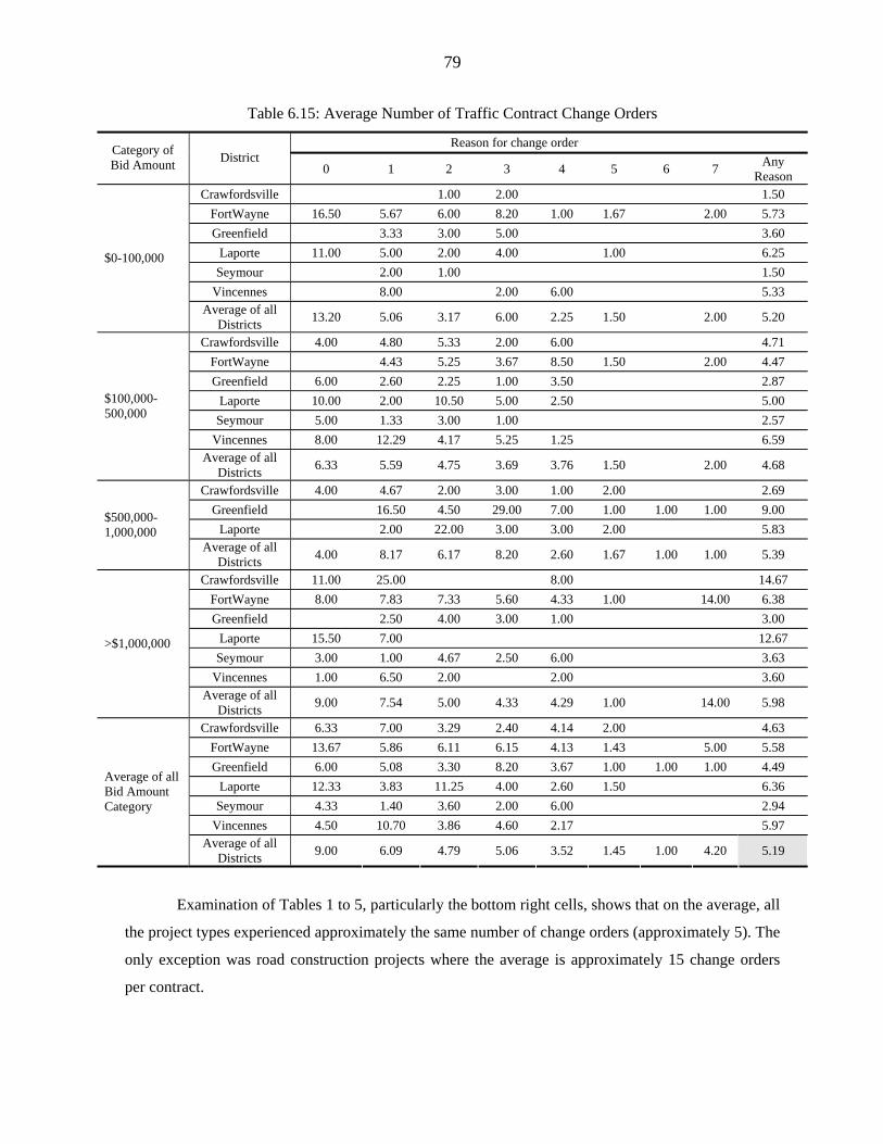
79
Table 6.15: Average Number of Traffic Contract Change Orders
Reason for change order Category of Bid Amount District
0 1 2 3 4 5 6 7 Any Reason
Crawfordsville 1.00 2.00 1.50 FortWayne 16.50 5.67 6.00 8.20 1.00 1.67 2.00 5.73 Greenfield 3.33 3.00 5.00 3.60
Laporte 11.00 5.00 2.00 4.00 1.00 6.25 Seymour 2.00 1.00 1.50
Vincennes 8.00 2.00 6.00 5.33
$0-100,000
Average of all Districts 13.20 5.06 3.17 6.00 2.25 1.50 2.00 5.20
Crawfordsville 4.00 4.80 5.33 2.00 6.00 4.71 FortWayne 4.43 5.25 3.67 8.50 1.50 2.00 4.47 Greenfield 6.00 2.60 2.25 1.00 3.50 2.87
Laporte 10.00 2.00 10.50 5.00 2.50 5.00 Seymour 5.00 1.33 3.00 1.00 2.57
Vincennes 8.00 12.29 4.17 5.25 1.25 6.59
$100,000-500,000
Average of all Districts 6.33 5.59 4.75 3.69 3.76 1.50 2.00 4.68
Crawfordsville 4.00 4.67 2.00 3.00 1.00 2.00 2.69 Greenfield 16.50 4.50 29.00 7.00 1.00 1.00 1.00 9.00
Laporte 2.00 22.00 3.00 3.00 2.00 5.83 $500,000-1,000,000
Average of all Districts 4.00 8.17 6.17 8.20 2.60 1.67 1.00 1.00 5.39
Crawfordsville 11.00 25.00 8.00 14.67 FortWayne 8.00 7.83 7.33 5.60 4.33 1.00 14.00 6.38 Greenfield 2.50 4.00 3.00 1.00 3.00
Laporte 15.50 7.00 12.67 Seymour 3.00 1.00 4.67 2.50 6.00 3.63
Vincennes 1.00 6.50 2.00 2.00 3.60
>$1,000,000
Average of all Districts 9.00 7.54 5.00 4.33 4.29 1.00 14.00 5.98
Crawfordsville 6.33 7.00 3.29 2.40 4.14 2.00 4.63 FortWayne 13.67 5.86 6.11 6.15 4.13 1.43 5.00 5.58 Greenfield 6.00 5.08 3.30 8.20 3.67 1.00 1.00 1.00 4.49
Laporte 12.33 3.83 11.25 4.00 2.60 1.50 6.36 Seymour 4.33 1.40 3.60 2.00 6.00 2.94
Vincennes 4.50 10.70 3.86 4.60 2.17 5.97
Average of all Bid Amount Category
Average of all Districts 9.00 6.09 4.79 5.06 3.52 1.45 1.00 4.20 5.19
Examination of Tables 1 to 5, particularly the bottom right cells, shows that on the average, all
the project types experienced approximately the same number of change orders (approximately 5). The
only exception was road construction projects where the average is approximately 15 change orders
per contract.
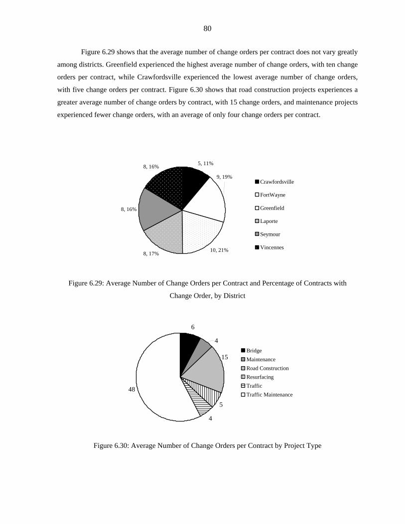
80
Figure 6.29 shows that the average number of change orders per contract does not vary greatly
among districts. Greenfield experienced the highest average number of change orders, with ten change
orders per contract, while Crawfordsville experienced the lowest average number of change orders,
with five change orders per contract. Figure 6.30 shows that road construction projects experiences a
greater average number of change orders by contract, with 15 change orders, and maintenance projects
experienced fewer change orders, with an average of only four change orders per contract.
5, 11%
10, 21%8, 17%
8, 16%
8, 16%
9, 19%Crawfordsville
FortWayne
Greenfield
Laporte
Seymour
Vincennes
Figure 6.29: Average Number of Change Orders per Contract and Percentage of Contracts with
Change Order, by District
6
5
4
48
15
4BridgeMaintenanceRoad ConstructionResurfacingTrafficTraffic Maintenance
Figure 6.30: Average Number of Change Orders per Contract by Project Type
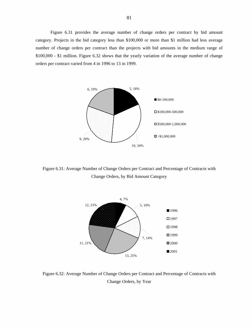
81
Figure 6.31 provides the average number of change orders per contract by bid amount
category. Projects in the bid category less than $100,000 or more than $1 million had less average
number of change orders per contract than the projects with bid amounts in the medium range of
$100,000 - $1 million. Figure 6.32 shows that the yearly variation of the average number of change
orders per contract varied from 4 in 1996 to 13 in 1999.
5, 18%6, 19%
9, 29%
10, 34%
$0-100,000
$100,000-500,000
$500,000-1,000,000
>$1,000,000
Figure 6.31: Average Number of Change Orders per Contract and Percentage of Contracts with
Change Orders, by Bid Amount Category
4, 7%
13, 25%
11, 21%
12, 23%
7, 14%
5, 10%1996
1997
1998
1999
2000
2001
Figure 6.32: Average Number of Change Orders per Contract and Percentage of Contracts with
Change Orders, by Year
82
Appendix E provides further detailed information on change orders. A comparison of the
average frequency of change orders per contract by project type and by district shows that Greenfield
bridge projects had the highest average number of change orders. For maintenance projects,
Crawfordsville had the highest average. In the six districts, road construction projects experienced
more change orders, with a much higher average (approximately 15 change orders), with no
particularly dominant district. For resurfacing projects, the Greenfield and Vincennes Districts had
more change orders per contract than the other district, and for traffic projects, the Seymour District is
had fewer change orders per contract. The “no reason” change order category was dominant in every
district, with only exception of Crawfordsville, where the proportion of “no reason” change orders was
much less than for the other districts. Concerning the other change order reason categories, the
Greenfield District had more “errors and omissions” and “constructability” change orders per contract.
Otherwise, there was little disparity among districts for change order reasons. Traffic projects seem to
experience less “no reason” change orders in proportion to other project types. Road construction
projects had the highest average number of change orders in the “errors and omissions,”
“constructability,” and “scope changes” categories.
6.6 Chapter Summary
The present chapter provided a discussion on the incidence of cost overruns, time delays, and
change orders in terms of their distribution by district, project type and bid amount category. Almost
half of the amount spent on change orders was associated with “no recorded reason.” If the “no
recorded reason” category is excluded, the “error and omission” category was the overwhelming
reason for change orders. Resurfacing projects experienced the most cost overruns, and maintenance
projects had the most time delay. The following chapter carries out detailed statistical analysis of cost
overruns, time delays, and change orders.
83
CHAPTER 7: STATISTICAL ANALYSIS I
7.1 Introduction
In discussing the distribution of cost overruns, time delays, and change order frequency by
project type, location, and bid amount category, the previous chapter laid the groundwork upon which
further statistical analysis could be carried out. The present chapter carries out preliminary statistical
investigations aimed at confirming identified trends between the dependent variables (cost overruns,
time delay and change order frequency) on one hand, and the potentially influential factors
(independent variables) on the other hand, and also to further establish a-priori expectations of the
strength and direction of such relationships. Four statistical tools were used to conduct the preliminary
statistical analysis. The correlation matrix was carried out to ascertain the existence of any linear
correlation between each pair of independent variables. The analysis of variance was carried out to
investigate any differences in the means of each dependent variables for various combinations of
levels of the potential influential factors. Then a pair-wise t-test was carried out to study any such
differences in a more precise manner. Finally, an analysis of the influence of each potentially
influential factor on the dependent variables was carried out.
7.2 Correlation Matrix
The correlation matrix between the independent variables provided in Table 7.1 showed the
Pearson correlation coefficient for each pair of variables. This statistic helped to identify any
correlations so that possible modeling biases from using correlated variables in the same model could
be avoided. Table 7.1 (where correlations are at 10% significance) shows that most of the Pearson
correlation coefficients were between -0.3 and 0.3. A notable exception is that for the variables
representing the proportion of the difference between the first and second bids and the proportion of
the difference between the lowest bid and the engineer’s estimate, which had a correlation coefficient
of 0.83 and is indicative of a strong positive association. As such, it was necessary to avoid using these
two variables in the same model or to exercise due caution where they had to be used in the same
model. For the other variables, there seemed to be no problem with correlation as their correlation
coefficients were sufficiently low.
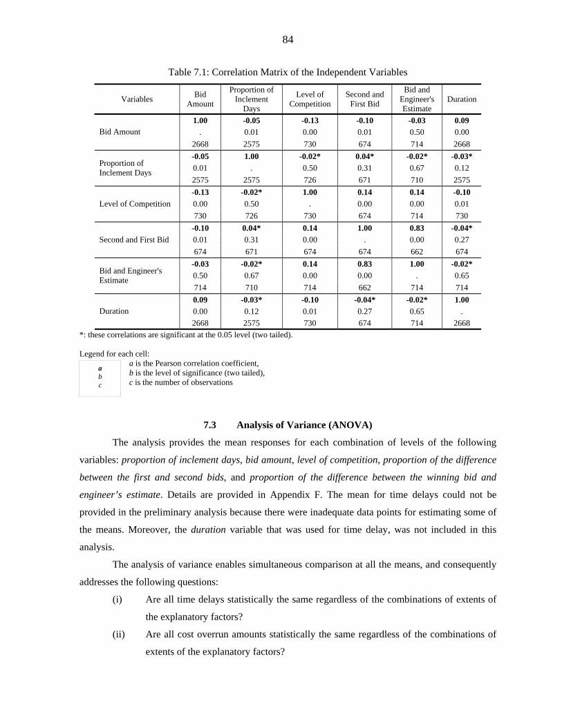
84
Table 7.1: Correlation Matrix of the Independent Variables
Variables Bid Amount
Proportion of Inclement
Days
Level of Competition
Second and First Bid
Bid and Engineer's Estimate
Duration
1.00 -0.05 -0.13 -0.10 -0.03 0.09 . 0.01 0.00 0.01 0.50 0.00 Bid Amount
2668 2575 730 674 714 2668 -0.05 1.00 -0.02* 0.04* -0.02* -0.03* 0.01 . 0.50 0.31 0.67 0.12 Proportion of
Inclement Days 2575 2575 726 671 710 2575 -0.13 -0.02* 1.00 0.14 0.14 -0.10 0.00 0.50 . 0.00 0.00 0.01 Level of Competition 730 726 730 674 714 730
-0.10 0.04* 0.14 1.00 0.83 -0.04* 0.01 0.31 0.00 . 0.00 0.27 Second and First Bid 674 671 674 674 662 674
-0.03 -0.02* 0.14 0.83 1.00 -0.02* 0.50 0.67 0.00 0.00 . 0.65 Bid and Engineer's
Estimate 714 710 714 662 714 714 0.09 -0.03* -0.10 -0.04* -0.02* 1.00 0.00 0.12 0.01 0.27 0.65 . Duration 2668 2575 730 674 714 2668
*: these correlations are significant at the 0.05 level (two tailed). Legend for each cell:
a is the Pearson correlation coefficient, b is the level of significance (two tailed), c is the number of observations
7.3 Analysis of Variance (ANOVA)
The analysis provides the mean responses for each combination of levels of the following
variables: proportion of inclement days, bid amount, level of competition, proportion of the difference
between the first and second bids, and proportion of the difference between the winning bid and
engineer’s estimate. Details are provided in Appendix F. The mean for time delays could not be
provided in the preliminary analysis because there were inadequate data points for estimating some of
the means. Moreover, the duration variable that was used for time delay, was not included in this
analysis.
The analysis of variance enables simultaneous comparison at all the means, and consequently
addresses the following questions:
(i) Are all time delays statistically the same regardless of the combinations of extents of
the explanatory factors?
(ii) Are all cost overrun amounts statistically the same regardless of the combinations of
extents of the explanatory factors?
a b c
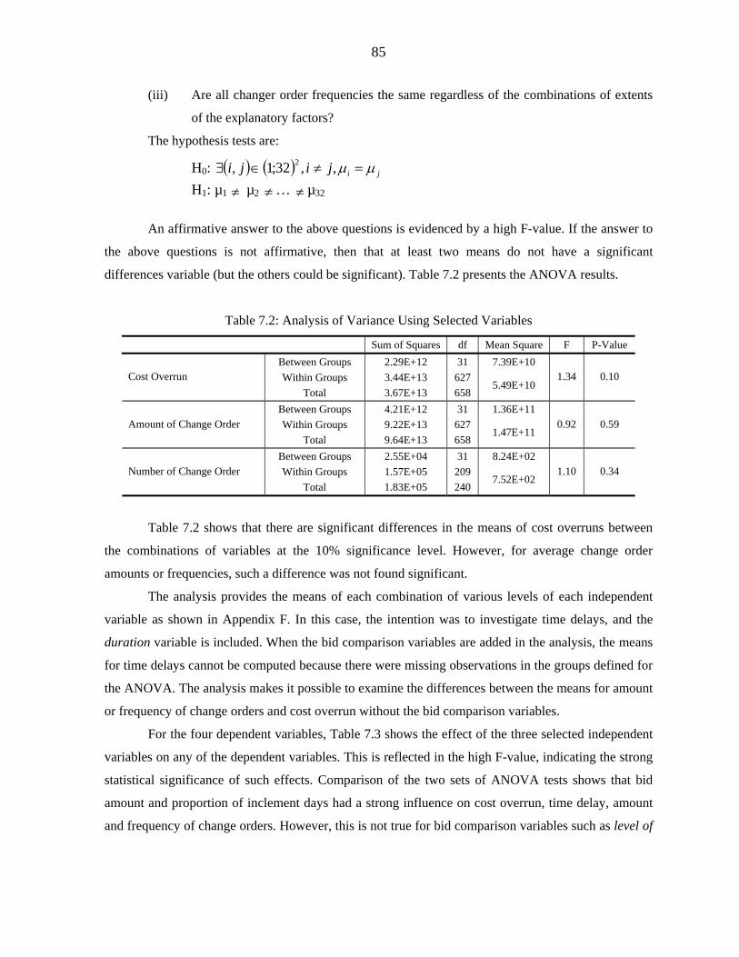
85
(iii) Are all changer order frequencies the same regardless of the combinations of extents
of the explanatory factors?
The hypothesis tests are:
H0: ( ) ( ) jijiji µµ =≠∈∃ ,,32;1, 2 H1: µ1 ≠ µ2 ≠ … ≠ µ32
An affirmative answer to the above questions is evidenced by a high F-value. If the answer to
the above questions is not affirmative, then that at least two means do not have a significant
differences variable (but the others could be significant). Table 7.2 presents the ANOVA results.
Table 7.2: Analysis of Variance Using Selected Variables
Sum of Squares df Mean Square F P-Value Between Groups 2.29E+12 31 7.39E+10 Within Groups 3.44E+13 627 Cost Overrun
Total 3.67E+13 658 5.49E+10
1.34 0.10
Between Groups 4.21E+12 31 1.36E+11 Within Groups 9.22E+13 627 Amount of Change Order
Total 9.64E+13 658 1.47E+11
0.92 0.59
Between Groups 2.55E+04 31 8.24E+02 Within Groups 1.57E+05 209 Number of Change Order
Total 1.83E+05 240 7.52E+02
1.10 0.34
Table 7.2 shows that there are significant differences in the means of cost overruns between
the combinations of variables at the 10% significance level. However, for average change order
amounts or frequencies, such a difference was not found significant.
The analysis provides the means of each combination of various levels of each independent
variable as shown in Appendix F. In this case, the intention was to investigate time delays, and the
duration variable is included. When the bid comparison variables are added in the analysis, the means
for time delays cannot be computed because there were missing observations in the groups defined for
the ANOVA. The analysis makes it possible to examine the differences between the means for amount
or frequency of change orders and cost overrun without the bid comparison variables.
For the four dependent variables, Table 7.3 shows the effect of the three selected independent
variables on any of the dependent variables. This is reflected in the high F-value, indicating the strong
statistical significance of such effects. Comparison of the two sets of ANOVA tests shows that bid
amount and proportion of inclement days had a strong influence on cost overrun, time delay, amount
and frequency of change orders. However, this is not true for bid comparison variables such as level of
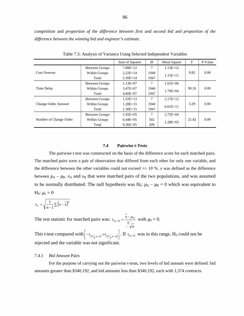
86
competition and proportion of the difference between first and second bid and proportion of the
difference between the winning bid and engineer’s estimate.
Table 7.3: Analysis of Variance Using Selected Independent Variables
Sum of Squares df Mean Square F P-Value Between Groups 7.88E+12 7 1.13E+12 Within Groups 2.22E+14 1940 Cost Overrun
Total 2.30E+14 1947 1.15E+11
9.82 0.00
Between Groups 1.13E+07 7 1.61E+06 Within Groups 3.47E+07 1940 Time Delay
Total 4.60E+07 1947 1.79E+04
90.16 0.00
Between Groups 1.52E+13 7 2.17E+12 Within Groups 1.28E+15 1940 Change Order Amount
Total 1.30E+15 1947 6.61E+11
3.29 0.00
Between Groups 1.92E+05 7 2.75E+04 Within Groups 6.44E+05 502 Number of Change Order
Total 8.36E+05 509 1.28E+03
21.42 0.00
7.4 Pairwise t-Tests
The pairwise t-test was constructed on the basis of the difference score for each matched pairs.
The matched pairs were a pair of observation that differed from each other for only one variable, and
the difference between the other variables could not exceed +/- 10 %. x was defined as the difference
between µA – µB. xA and xB that were matched pairs of the two populations, and was assumed
to be normally distributed. The null hypothesis was H0: µA – µB = 0 which was equivalent to
H0: µx = 0
( )∑ −−
=2
11 xx
nsx
The test statistic for matched pairs was: n
sx
t n0
)1(µ−
=− with µ0 = 0.
This t-test compared with ⎥⎦⎤
⎢⎣⎡ +−
−− )1,2()1,2( ; nn tt αα . If )1( −nt was in this range, H0 could not be
rejected and the variable was not significant.
7.4.1 Bid Amount Pairs
For the purpose of carrying out the pairwise t-tests, two levels of bid amount were defined: bid
amounts greater than $340,192, and bid amounts less than $340,192, each with 1,374 contracts.
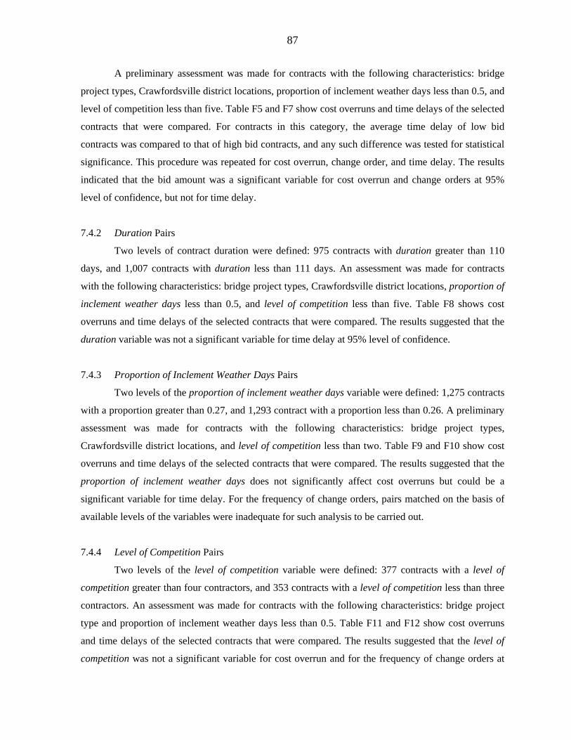
87
A preliminary assessment was made for contracts with the following characteristics: bridge
project types, Crawfordsville district locations, proportion of inclement weather days less than 0.5, and
level of competition less than five. Table F5 and F7 show cost overruns and time delays of the selected
contracts that were compared. For contracts in this category, the average time delay of low bid
contracts was compared to that of high bid contracts, and any such difference was tested for statistical
significance. This procedure was repeated for cost overrun, change order, and time delay. The results
indicated that the bid amount was a significant variable for cost overrun and change orders at 95%
level of confidence, but not for time delay.
7.4.2 Duration Pairs
Two levels of contract duration were defined: 975 contracts with duration greater than 110
days, and 1,007 contracts with duration less than 111 days. An assessment was made for contracts
with the following characteristics: bridge project types, Crawfordsville district locations, proportion of
inclement weather days less than 0.5, and level of competition less than five. Table F8 shows cost
overruns and time delays of the selected contracts that were compared. The results suggested that the
duration variable was not a significant variable for time delay at 95% level of confidence.
7.4.3 Proportion of Inclement Weather Days Pairs
Two levels of the proportion of inclement weather days variable were defined: 1,275 contracts
with a proportion greater than 0.27, and 1,293 contract with a proportion less than 0.26. A preliminary
assessment was made for contracts with the following characteristics: bridge project types,
Crawfordsville district locations, and level of competition less than two. Table F9 and F10 show cost
overruns and time delays of the selected contracts that were compared. The results suggested that the
proportion of inclement weather days does not significantly affect cost overruns but could be a
significant variable for time delay. For the frequency of change orders, pairs matched on the basis of
available levels of the variables were inadequate for such analysis to be carried out.
7.4.4 Level of Competition Pairs
Two levels of the level of competition variable were defined: 377 contracts with a level of
competition greater than four contractors, and 353 contracts with a level of competition less than three
contractors. An assessment was made for contracts with the following characteristics: bridge project
type and proportion of inclement weather days less than 0.5. Table F11 and F12 show cost overruns
and time delays of the selected contracts that were compared. The results suggested that the level of
competition was not a significant variable for cost overrun and for the frequency of change orders at
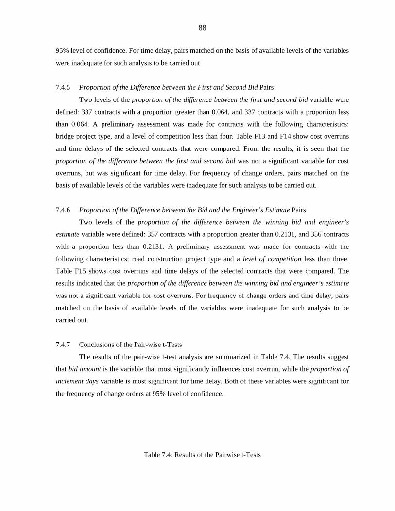
88
95% level of confidence. For time delay, pairs matched on the basis of available levels of the variables
were inadequate for such analysis to be carried out.
7.4.5 Proportion of the Difference between the First and Second Bid Pairs
Two levels of the proportion of the difference between the first and second bid variable were
defined: 337 contracts with a proportion greater than 0.064, and 337 contracts with a proportion less
than 0.064. A preliminary assessment was made for contracts with the following characteristics:
bridge project type, and a level of competition less than four. Table F13 and F14 show cost overruns
and time delays of the selected contracts that were compared. From the results, it is seen that the
proportion of the difference between the first and second bid was not a significant variable for cost
overruns, but was significant for time delay. For frequency of change orders, pairs matched on the
basis of available levels of the variables were inadequate for such analysis to be carried out.
7.4.6 Proportion of the Difference between the Bid and the Engineer’s Estimate Pairs
Two levels of the proportion of the difference between the winning bid and engineer’s
estimate variable were defined: 357 contracts with a proportion greater than 0.2131, and 356 contracts
with a proportion less than 0.2131. A preliminary assessment was made for contracts with the
following characteristics: road construction project type and a level of competition less than three.
Table F15 shows cost overruns and time delays of the selected contracts that were compared. The
results indicated that the proportion of the difference between the winning bid and engineer’s estimate
was not a significant variable for cost overruns. For frequency of change orders and time delay, pairs
matched on the basis of available levels of the variables were inadequate for such analysis to be
carried out.
7.4.7 Conclusions of the Pair-wise t-Tests
The results of the pair-wise t-test analysis are summarized in Table 7.4. The results suggest
that bid amount is the variable that most significantly influences cost overrun, while the proportion of
inclement days variable is most significant for time delay. Both of these variables were significant for
the frequency of change orders at 95% level of confidence.
Table 7.4: Results of the Pairwise t-Tests
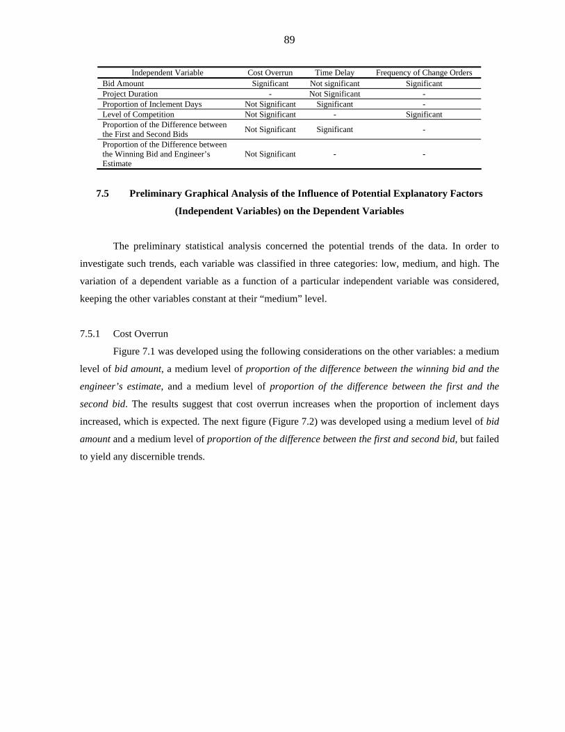
89
Independent Variable Cost Overrun Time Delay Frequency of Change Orders Bid Amount Significant Not significant Significant Project Duration - Not Significant - Proportion of Inclement Days Not Significant Significant - Level of Competition Not Significant - Significant Proportion of the Difference between the First and Second Bids Not Significant Significant -
Proportion of the Difference between the Winning Bid and Engineer’s Estimate
Not Significant - -
7.5 Preliminary Graphical Analysis of the Influence of Potential Explanatory Factors
(Independent Variables) on the Dependent Variables
The preliminary statistical analysis concerned the potential trends of the data. In order to
investigate such trends, each variable was classified in three categories: low, medium, and high. The
variation of a dependent variable as a function of a particular independent variable was considered,
keeping the other variables constant at their “medium” level.
7.5.1 Cost Overrun
Figure 7.1 was developed using the following considerations on the other variables: a medium
level of bid amount, a medium level of proportion of the difference between the winning bid and the
engineer’s estimate, and a medium level of proportion of the difference between the first and the
second bid. The results suggest that cost overrun increases when the proportion of inclement days
increased, which is expected. The next figure (Figure 7.2) was developed using a medium level of bid
amount and a medium level of proportion of the difference between the first and second bid, but failed
to yield any discernible trends.
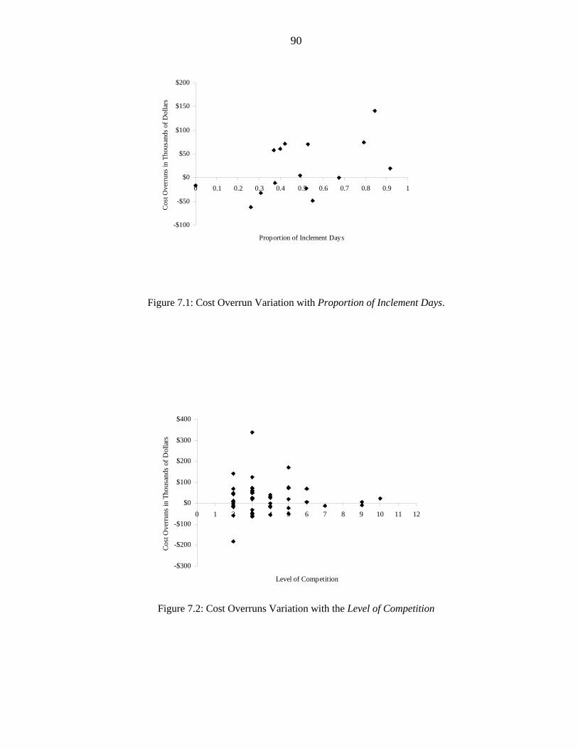
90
-$100
-$50
$0
$50
$100
$150
$200
0 0.1 0.2 0.3 0.4 0.5 0.6 0.7 0.8 0.9 1
Proportion of Inclement Days
Cos
t Ove
rrun
s in
Tho
usan
ds o
f Dol
lars
Figure 7.1: Cost Overrun Variation with Proportion of Inclement Days.
-$300
-$200
-$100
$0
$100
$200
$300
$400
0 1 2 3 4 5 6 7 8 9 10 11 12
Level of Competition
Cos
t Ove
rrun
s in
Tho
usan
ds o
f Dol
lars
Figure 7.2: Cost Overruns Variation with the Level of Competition
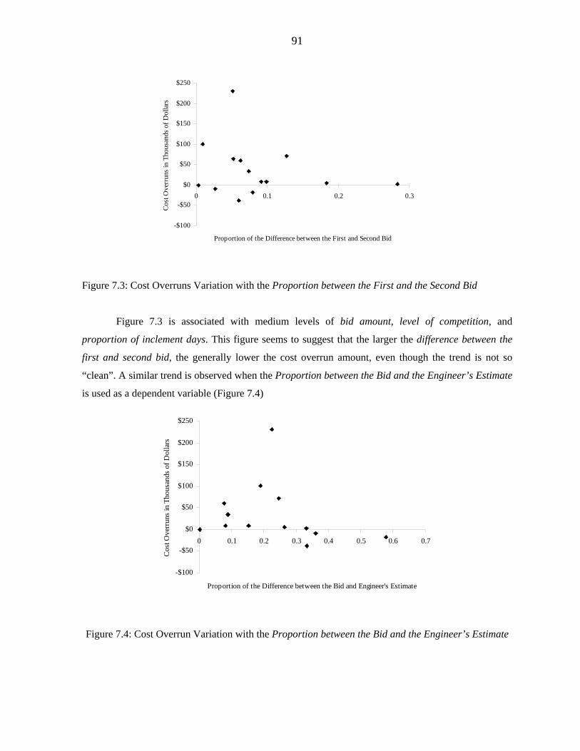
91
-$100
-$50
$0
$50
$100
$150
$200
$250
0 0.1 0.2 0.3
Proportion of the Difference between the First and Second Bid
Cos
t Ove
rrun
s in
Tho
usan
ds o
f Dol
lars
Figure 7.3: Cost Overruns Variation with the Proportion between the First and the Second Bid
Figure 7.3 is associated with medium levels of bid amount, level of competition, and
proportion of inclement days. This figure seems to suggest that the larger the difference between the
first and second bid, the generally lower the cost overrun amount, even though the trend is not so
“clean”. A similar trend is observed when the Proportion between the Bid and the Engineer’s Estimate
is used as a dependent variable (Figure 7.4)
-$100
-$50
$0
$50
$100
$150
$200
$250
0 0.1 0.2 0.3 0.4 0.5 0.6 0.7
Proportion of the Difference between the Bid and Engineer's Estimate
Cos
t Ove
rrun
s in
Tho
usan
ds o
f Dol
lars
Figure 7.4: Cost Overrun Variation with the Proportion between the Bid and the Engineer’s Estimate
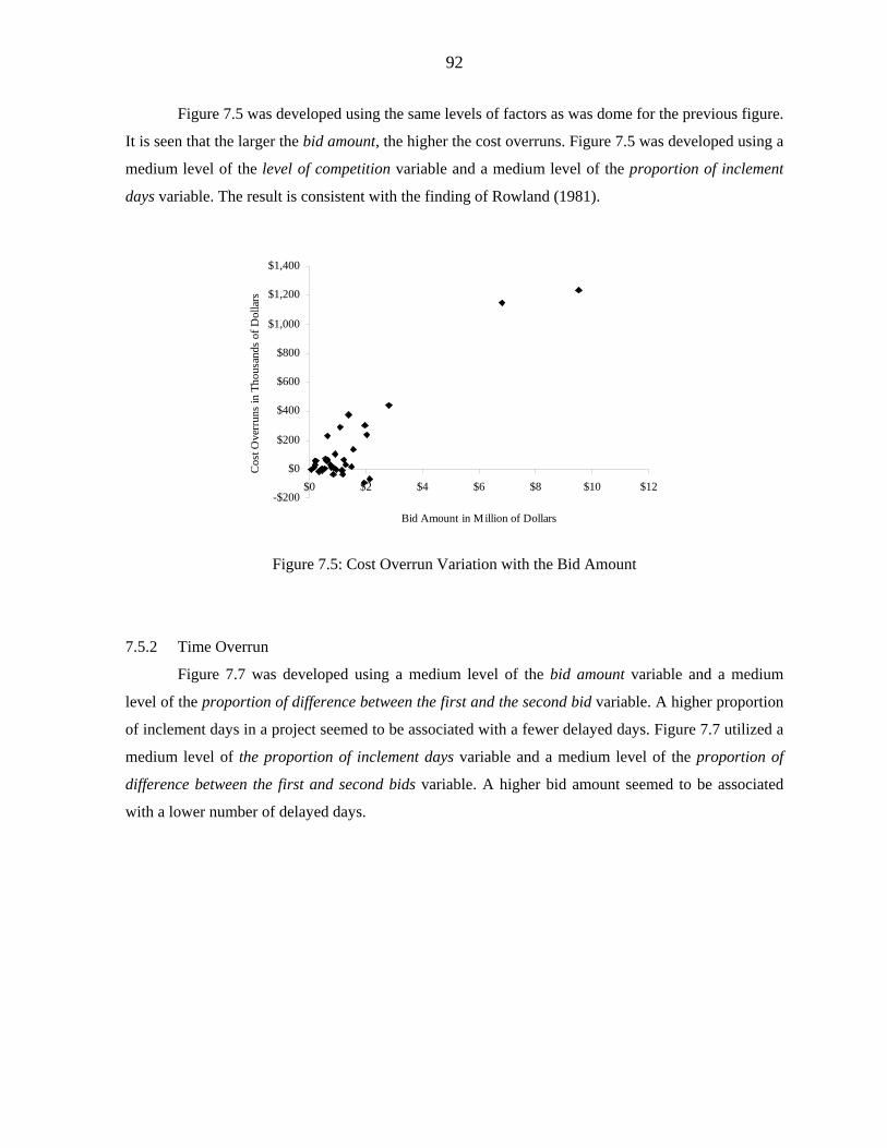
92
Figure 7.5 was developed using the same levels of factors as was dome for the previous figure.
It is seen that the larger the bid amount, the higher the cost overruns. Figure 7.5 was developed using a
medium level of the level of competition variable and a medium level of the proportion of inclement
days variable. The result is consistent with the finding of Rowland (1981).
-$200
$0
$200
$400
$600
$800
$1,000
$1,200
$1,400
$0 $2 $4 $6 $8 $10 $12
Bid Amount in Million of Dollars
Cos
t Ove
rrun
s in
Tho
usan
ds o
f Dol
lars
Figure 7.5: Cost Overrun Variation with the Bid Amount
7.5.2 Time Overrun
Figure 7.7 was developed using a medium level of the bid amount variable and a medium
level of the proportion of difference between the first and the second bid variable. A higher proportion
of inclement days in a project seemed to be associated with a fewer delayed days. Figure 7.7 utilized a
medium level of the proportion of inclement days variable and a medium level of the proportion of
difference between the first and second bids variable. A higher bid amount seemed to be associated
with a lower number of delayed days.
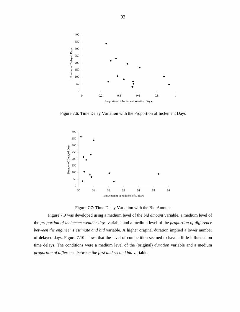
93
0
50
100
150
200
250
300
350
400
0 0.2 0.4 0.6 0.8 1
Proportion of Inclement Weather Days
Num
ber o
f Del
ayed
Day
s
Figure 7.6: Time Delay Variation with the Proportion of Inclement Days
0
50
100
150
200
250
300
350
400
$0 $1 $2 $3 $4 $5 $6
Bid Amount in Millions of Dollars
Num
ber o
f Del
ayed
Day
s
Figure 7.7: Time Delay Variation with the Bid Amount
Figure 7.9 was developed using a medium level of the bid amount variable, a medium level of
the proportion of inclement weather days variable and a medium level of the proportion of difference
between the engineer’s estimate and bid variable. A higher original duration implied a lower number
of delayed days. Figure 7.10 shows that the level of competition seemed to have a little influence on
time delays. The conditions were a medium level of the (original) duration variable and a medium
proportion of difference between the first and second bid variable.
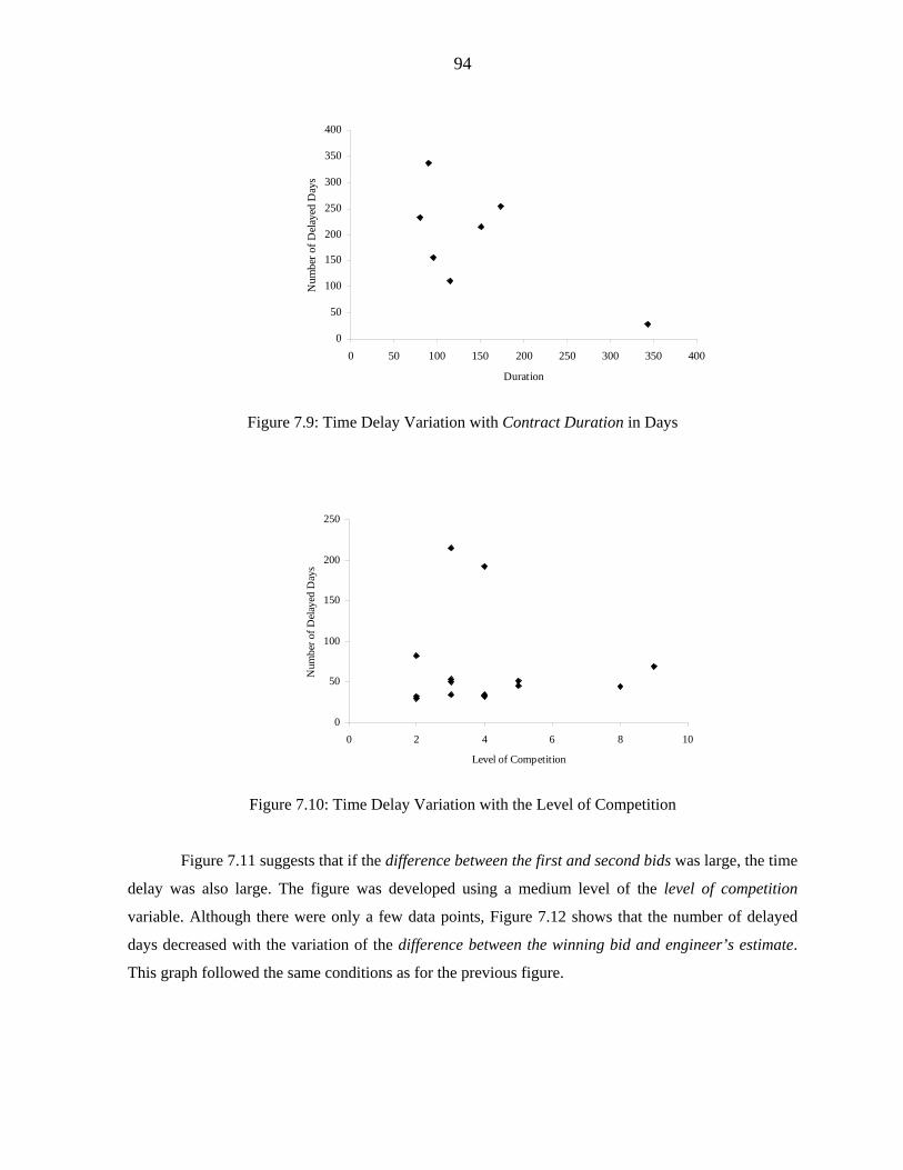
94
0
50
100
150
200
250
300
350
400
0 50 100 150 200 250 300 350 400
Duration
Num
ber o
f Del
ayed
Day
s
Figure 7.9: Time Delay Variation with Contract Duration in Days
0
50
100
150
200
250
0 2 4 6 8 10
Level of Competition
Num
ber o
f Del
ayed
Day
s
Figure 7.10: Time Delay Variation with the Level of Competition
Figure 7.11 suggests that if the difference between the first and second bids was large, the time
delay was also large. The figure was developed using a medium level of the level of competition
variable. Although there were only a few data points, Figure 7.12 shows that the number of delayed
days decreased with the variation of the difference between the winning bid and engineer’s estimate.
This graph followed the same conditions as for the previous figure.
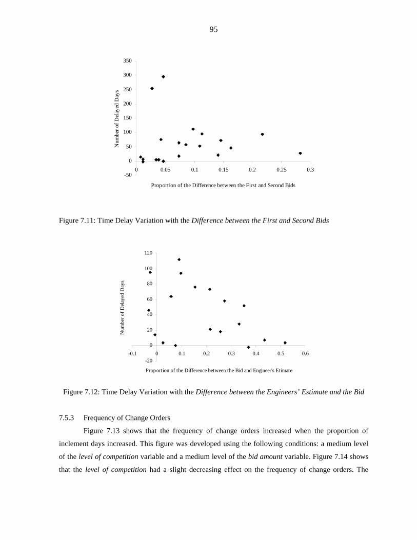
95
-50
0
50
100
150
200
250
300
350
0 0.05 0.1 0.15 0.2 0.25 0.3
Proportion of the Difference between the First and Second Bids
Num
ber o
f Del
ayed
Day
s
Figure 7.11: Time Delay Variation with the Difference between the First and Second Bids
-20
0
20
40
60
80
100
120
-0.1 0 0.1 0.2 0.3 0.4 0.5 0.6
Proportion of the Difference between the Bid and Engineer's Etimate
Num
ber o
f Del
ayed
Day
s
Figure 7.12: Time Delay Variation with the Difference between the Engineers’ Estimate and the Bid
7.5.3 Frequency of Change Orders
Figure 7.13 shows that the frequency of change orders increased when the proportion of
inclement days increased. This figure was developed using the following conditions: a medium level
of the level of competition variable and a medium level of the bid amount variable. Figure 7.14 shows
that the level of competition had a slight decreasing effect on the frequency of change orders. The
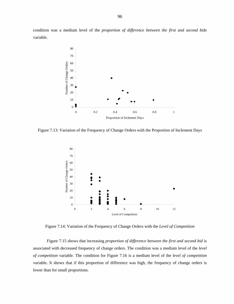
96
condition was a medium level of the proportion of difference between the first and second bids
variable.
0
10
20
30
40
50
60
70
80
0 0.2 0.4 0.6 0.8 1
Proportion of Inclement Days
Num
ber o
f Cha
nge
Ord
ers
Figure 7.13: Variation of the Frequency of Change Orders with the Proportion of Inclement Days
0
10
20
30
40
50
60
70
80
0 2 4 6 8 10 12
Level of Competition
Num
ber o
f Cha
nge
Ord
ers
Figure 7.14: Variation of the Frequency of Change Orders with the Level of Competition
Figure 7.15 shows that increasing proportion of difference between the first and second bid is
associated with decreased frequency of change orders. The condition was a medium level of the level
of competition variable. The condition for Figure 7.16 is a medium level of the level of competition
variable. It shows that if this proportion of difference was high, the frequency of change orders is
lower than for small proportions.
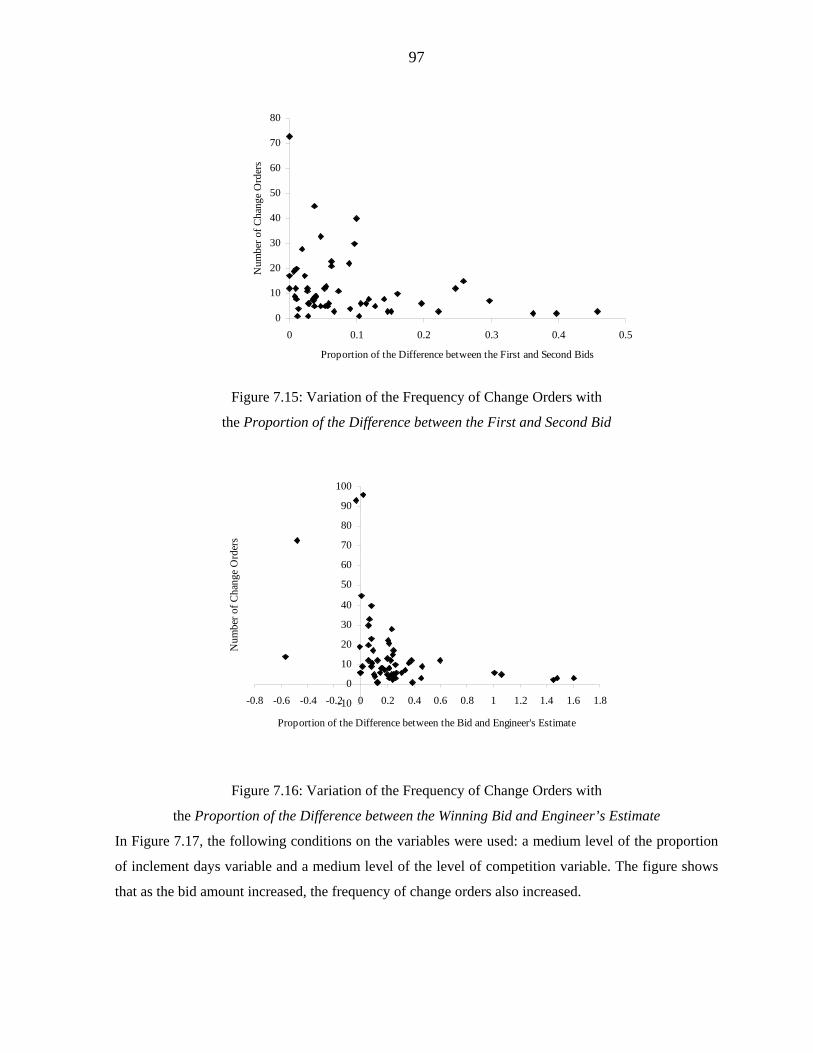
97
0
10
20
30
40
50
60
70
80
0 0.1 0.2 0.3 0.4 0.5
Proportion of the Difference between the First and Second Bids
Num
ber o
f Cha
nge
Ord
ers
Figure 7.15: Variation of the Frequency of Change Orders with
the Proportion of the Difference between the First and Second Bid
-10
0
10
20
30
40
50
60
70
80
90
100
-0.8 -0.6 -0.4 -0.2 0 0.2 0.4 0.6 0.8 1 1.2 1.4 1.6 1.8
Proportion of the Difference between the Bid and Engineer's Estimate
Num
ber o
f Cha
nge
Ord
ers
Figure 7.16: Variation of the Frequency of Change Orders with
the Proportion of the Difference between the Winning Bid and Engineer’s Estimate
In Figure 7.17, the following conditions on the variables were used: a medium level of the proportion
of inclement days variable and a medium level of the level of competition variable. The figure shows
that as the bid amount increased, the frequency of change orders also increased.
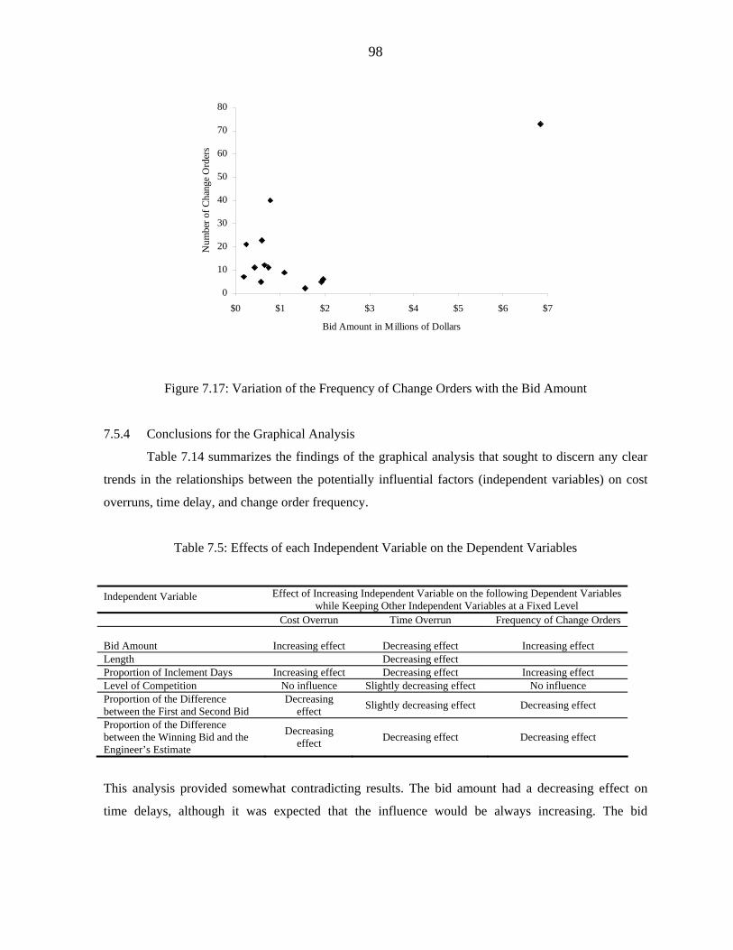
98
0
10
20
30
40
50
60
70
80
$0 $1 $2 $3 $4 $5 $6 $7
Bid Amount in Millions of Dollars
Num
ber o
f Cha
nge
Ord
ers
Figure 7.17: Variation of the Frequency of Change Orders with the Bid Amount
7.5.4 Conclusions for the Graphical Analysis
Table 7.14 summarizes the findings of the graphical analysis that sought to discern any clear
trends in the relationships between the potentially influential factors (independent variables) on cost
overruns, time delay, and change order frequency.
Table 7.5: Effects of each Independent Variable on the Dependent Variables
Independent Variable Effect of Increasing Independent Variable on the following Dependent Variables while Keeping Other Independent Variables at a Fixed Level
Cost Overrun Time Overrun Frequency of Change Orders Bid Amount
Increasing effect
Decreasing effect
Increasing effect
Length Decreasing effect Proportion of Inclement Days Increasing effect Decreasing effect Increasing effect Level of Competition No influence Slightly decreasing effect No influence Proportion of the Difference between the First and Second Bid
Decreasing effect Slightly decreasing effect Decreasing effect
Proportion of the Difference between the Winning Bid and the Engineer’s Estimate
Decreasing effect Decreasing effect Decreasing effect
This analysis provided somewhat contradicting results. The bid amount had a decreasing effect on
time delays, although it was expected that the influence would be always increasing. The bid
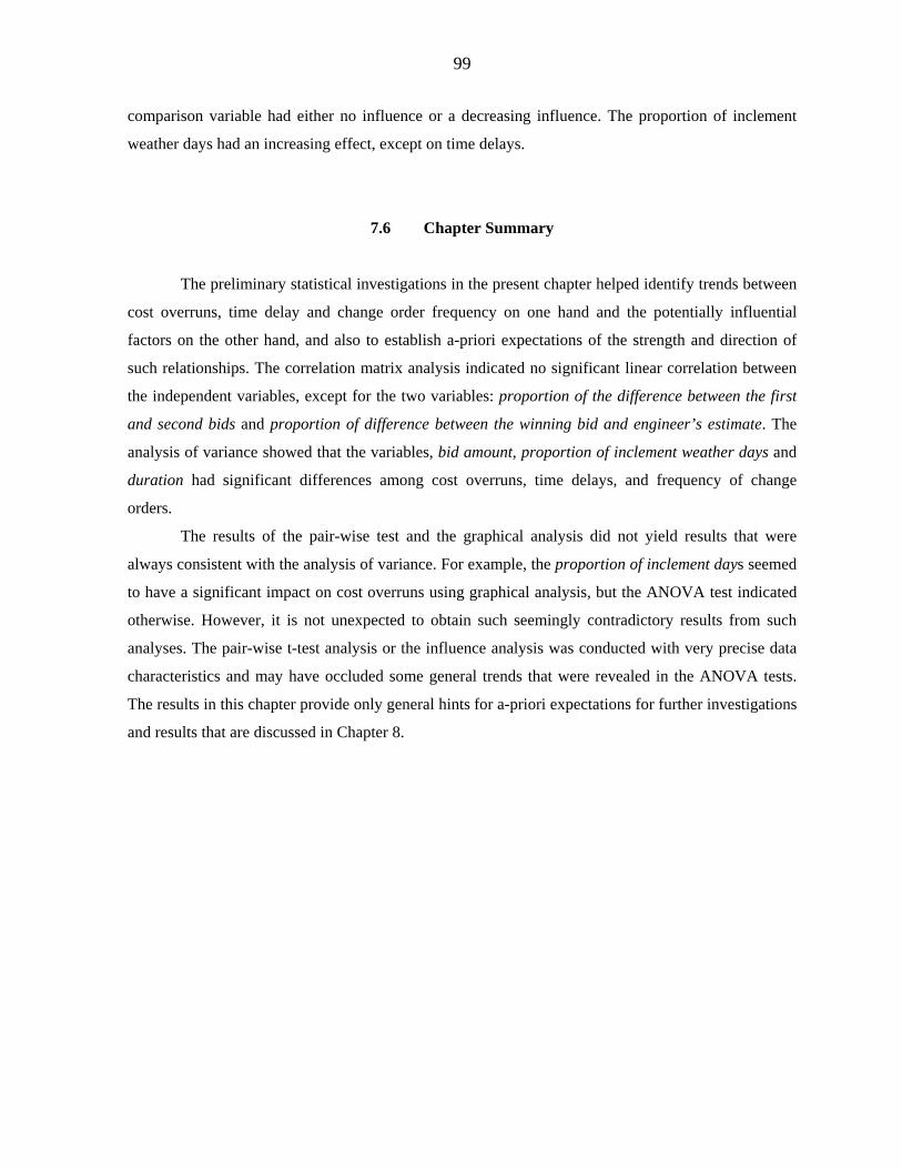
99
comparison variable had either no influence or a decreasing influence. The proportion of inclement
weather days had an increasing effect, except on time delays.
7.6 Chapter Summary
The preliminary statistical investigations in the present chapter helped identify trends between
cost overruns, time delay and change order frequency on one hand and the potentially influential
factors on the other hand, and also to establish a-priori expectations of the strength and direction of
such relationships. The correlation matrix analysis indicated no significant linear correlation between
the independent variables, except for the two variables: proportion of the difference between the first
and second bids and proportion of difference between the winning bid and engineer’s estimate. The
analysis of variance showed that the variables, bid amount, proportion of inclement weather days and
duration had significant differences among cost overruns, time delays, and frequency of change
orders.
The results of the pair-wise test and the graphical analysis did not yield results that were
always consistent with the analysis of variance. For example, the proportion of inclement days seemed
to have a significant impact on cost overruns using graphical analysis, but the ANOVA test indicated
otherwise. However, it is not unexpected to obtain such seemingly contradictory results from such
analyses. The pair-wise t-test analysis or the influence analysis was conducted with very precise data
characteristics and may have occluded some general trends that were revealed in the ANOVA tests.
The results in this chapter provide only general hints for a-priori expectations for further investigations
and results that are discussed in Chapter 8.
99
CHAPTER 8: STATISTICAL MODELS
8.1 Introduction
The present chapter investigates the influence of variables found significant from analyses
presented in the previous chapter. This is done for cost overrun, time delay, and change orders. It is
worth mentioning that the primary goal of the modeling process was to identify or confirm the
magnitude and direction of the impacts of the variables, while the use of the developed models for
prediction was considered only a secondary goal.
For each of the three response variables, two models were developed: one that included “bid
comparison” variables, and one that excluded such variables. Models that included the “bid
comparison” variables were developed using only those observations for which such data was
available, and therefore the dataset for such models was only a subset of the full dataset. Such models
are applicable in cases where bid have been received for a contract, and INDOT seeks to estimate the
expected cost overruns, time delay or change orders for the contract. Models that excluded the “bid
comparison” variables were developed using the entire dataset. Such models are applicable in cases
where no bids are yet available for a contract, and are therefore useful for long term planning and
estimation of expected cost overruns, time delay or change orders for contracts. The “ bid comparison”
variables are the proportion of the difference between the amounts for the winning bid and the second
bid, the proportion of the difference between the winning bid and the engineer’s estimate, and the level
of competition. Each model was validated using 25% of data points set aside for that purpose.
Figure 8.1 presents a schematic framework of the modeling process.
The strength and magnitude of factors affecting change order frequency and amounts, time
delay, and cost overrun amounts and rates, models were investigated using regression modeling.
Recognizing that efforts by INDOT to predict these parameters for future projects may be constrained
by lack of bidding information, separate models were attempted for cases where bid comparison
variables are available and where such variables are not available. The regression modeling was
carried out for each project type.
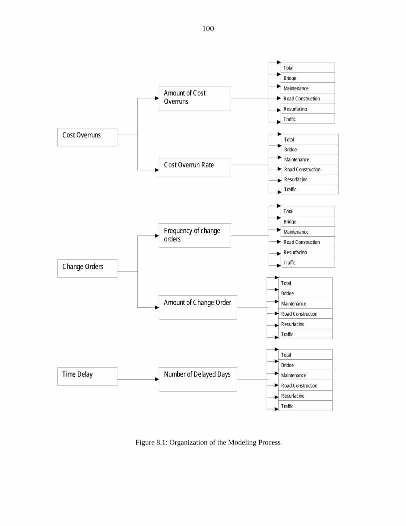
100
Figure 8.1: Organization of the Modeling Process
Cost Overruns
Amount of Cost Overruns
Cost Overrun Rate
Frequency of change orders
Amount of Change Order
Number of Delayed Days
Change Orders
Time Delay
Total
Bridge
Maintenance
Road Construction
Resurfacing
Traffic
Total
Bridge
Maintenance
Road Construction
Resurfacing
Traffic
Total
Bridge
Maintenance
Road Construction
Resurfacing
Traffic
Total
Bridge
Maintenance
Road Construction
Resurfacing
Traffic
Total
Bridge
Maintenance
Road Construction
Resurfacing
Traffic
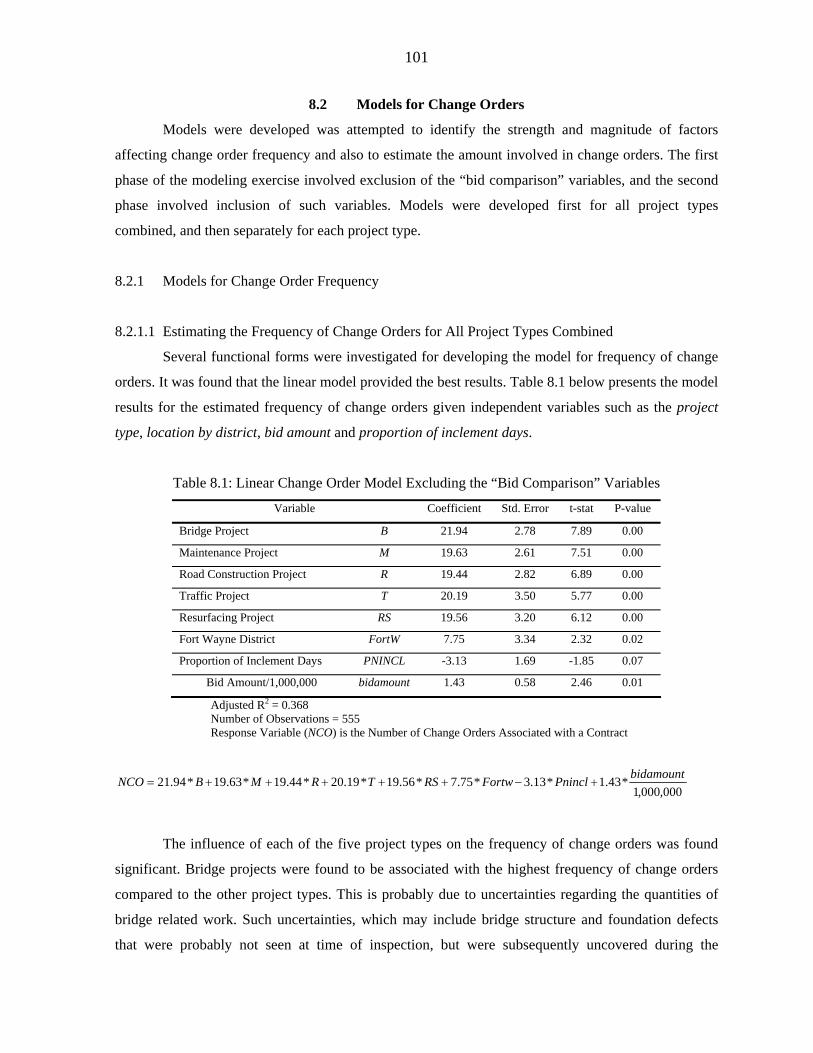
101
8.2 Models for Change Orders
Models were developed was attempted to identify the strength and magnitude of factors
affecting change order frequency and also to estimate the amount involved in change orders. The first
phase of the modeling exercise involved exclusion of the “bid comparison” variables, and the second
phase involved inclusion of such variables. Models were developed first for all project types
combined, and then separately for each project type.
8.2.1 Models for Change Order Frequency
8.2.1.1 Estimating the Frequency of Change Orders for All Project Types Combined
Several functional forms were investigated for developing the model for frequency of change
orders. It was found that the linear model provided the best results. Table 8.1 below presents the model
results for the estimated frequency of change orders given independent variables such as the project
type, location by district, bid amount and proportion of inclement days.
Table 8.1: Linear Change Order Model Excluding the “Bid Comparison” Variables
Variable Coefficient Std. Error t-stat P-value
Bridge Project B 21.94 2.78 7.89 0.00
Maintenance Project M 19.63 2.61 7.51 0.00
Road Construction Project R 19.44 2.82 6.89 0.00
Traffic Project T 20.19 3.50 5.77 0.00
Resurfacing Project RS 19.56 3.20 6.12 0.00
Fort Wayne District FortW 7.75 3.34 2.32 0.02
Proportion of Inclement Days PNINCL -3.13 1.69 -1.85 0.07
Bid Amount/1,000,000 bidamount 1.43 0.58 2.46 0.01
Adjusted R2 = 0.368 Number of Observations = 555 Response Variable (NCO) is the Number of Change Orders Associated with a Contract
000,000,1*43.1*13.3*75.7*56.19*19.20*44.19*63.19*94.21 bidamountPninclFortwRSTRMBNCO +−+++++=
The influence of each of the five project types on the frequency of change orders was found
significant. Bridge projects were found to be associated with the highest frequency of change orders
compared to the other project types. This is probably due to uncertainties regarding the quantities of
bridge related work. Such uncertainties, which may include bridge structure and foundation defects
that were probably not seen at time of inspection, but were subsequently uncovered during the
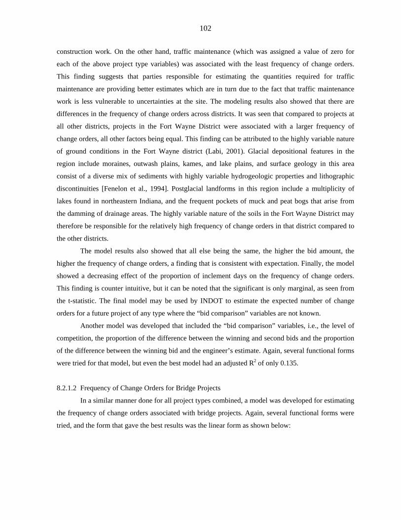
102
construction work. On the other hand, traffic maintenance (which was assigned a value of zero for
each of the above project type variables) was associated with the least frequency of change orders.
This finding suggests that parties responsible for estimating the quantities required for traffic
maintenance are providing better estimates which are in turn due to the fact that traffic maintenance
work is less vulnerable to uncertainties at the site. The modeling results also showed that there are
differences in the frequency of change orders across districts. It was seen that compared to projects at
all other districts, projects in the Fort Wayne District were associated with a larger frequency of
change orders, all other factors being equal. This finding can be attributed to the highly variable nature
of ground conditions in the Fort Wayne district (Labi, 2001). Glacial depositional features in the
region include moraines, outwash plains, kames, and lake plains, and surface geology in this area
consist of a diverse mix of sediments with highly variable hydrogeologic properties and lithographic
discontinuities [Fenelon et al., 1994]. Postglacial landforms in this region include a multiplicity of
lakes found in northeastern Indiana, and the frequent pockets of muck and peat bogs that arise from
the damming of drainage areas. The highly variable nature of the soils in the Fort Wayne District may
therefore be responsible for the relatively high frequency of change orders in that district compared to
the other districts.
The model results also showed that all else being the same, the higher the bid amount, the
higher the frequency of change orders, a finding that is consistent with expectation. Finally, the model
showed a decreasing effect of the proportion of inclement days on the frequency of change orders.
This finding is counter intuitive, but it can be noted that the significant is only marginal, as seen from
the t-statistic. The final model may be used by INDOT to estimate the expected number of change
orders for a future project of any type where the “bid comparison” variables are not known.
Another model was developed that included the “bid comparison” variables, i.e., the level of
competition, the proportion of the difference between the winning and second bids and the proportion
of the difference between the winning bid and the engineer’s estimate. Again, several functional forms
were tried for that model, but even the best model had an adjusted R2 of only 0.135.
8.2.1.2 Frequency of Change Orders for Bridge Projects
In a similar manner done for all project types combined, a model was developed for estimating
the frequency of change orders associated with bridge projects. Again, several functional forms were
tried, and the form that gave the best results was the linear form as shown below:
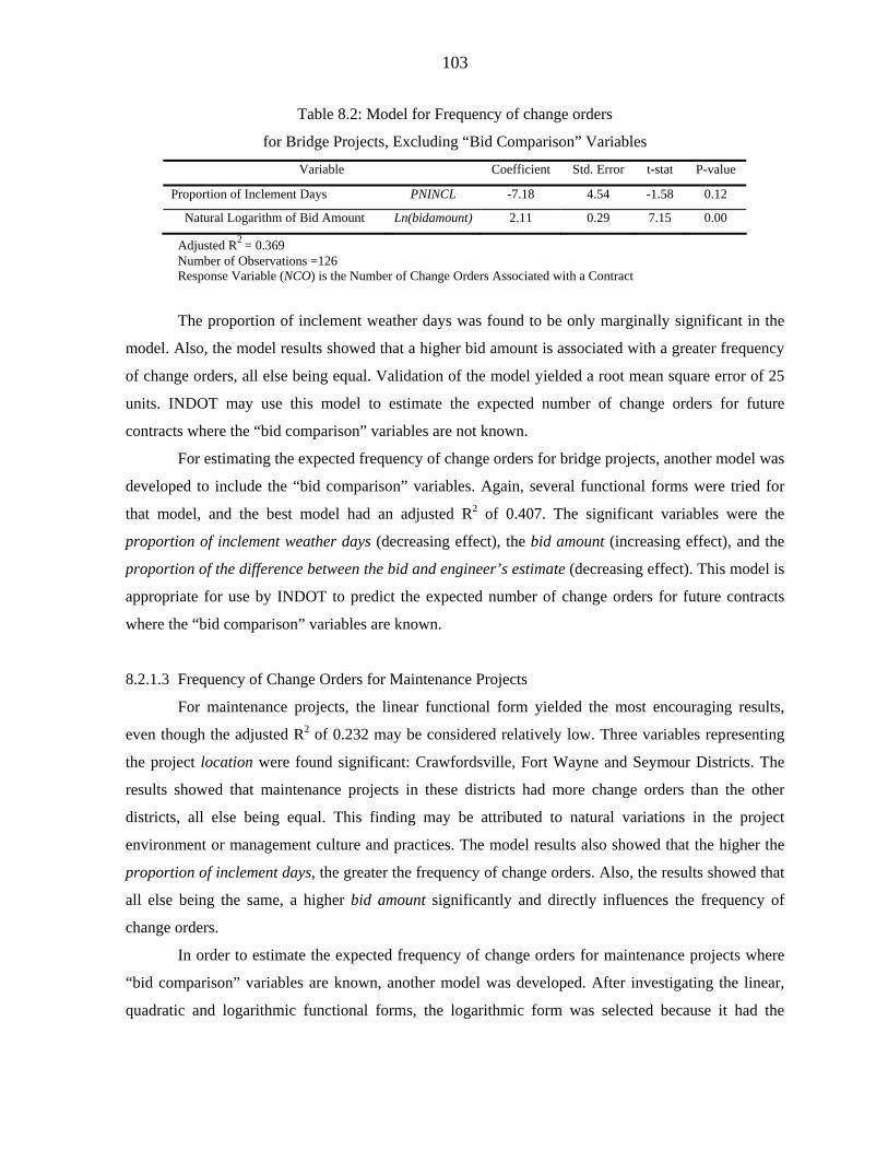
103
Table 8.2: Model for Frequency of change orders
for Bridge Projects, Excluding “Bid Comparison” Variables
Variable Coefficient Std. Error t-stat P-value
Proportion of Inclement Days PNINCL -7.18 4.54 -1.58 0.12
Natural Logarithm of Bid Amount Ln(bidamount) 2.11 0.29 7.15 0.00
Adjusted R2 = 0.369 Number of Observations =126 Response Variable (NCO) is the Number of Change Orders Associated with a Contract
The proportion of inclement weather days was found to be only marginally significant in the
model. Also, the model results showed that a higher bid amount is associated with a greater frequency
of change orders, all else being equal. Validation of the model yielded a root mean square error of 25
units. INDOT may use this model to estimate the expected number of change orders for future
contracts where the “bid comparison” variables are not known.
For estimating the expected frequency of change orders for bridge projects, another model was
developed to include the “bid comparison” variables. Again, several functional forms were tried for
that model, and the best model had an adjusted R2 of 0.407. The significant variables were the
proportion of inclement weather days (decreasing effect), the bid amount (increasing effect), and the
proportion of the difference between the bid and engineer’s estimate (decreasing effect). This model is
appropriate for use by INDOT to predict the expected number of change orders for future contracts
where the “bid comparison” variables are known.
8.2.1.3 Frequency of Change Orders for Maintenance Projects
For maintenance projects, the linear functional form yielded the most encouraging results,
even though the adjusted R2 of 0.232 may be considered relatively low. Three variables representing
the project location were found significant: Crawfordsville, Fort Wayne and Seymour Districts. The
results showed that maintenance projects in these districts had more change orders than the other
districts, all else being equal. This finding may be attributed to natural variations in the project
environment or management culture and practices. The model results also showed that the higher the
proportion of inclement days, the greater the frequency of change orders. Also, the results showed that
all else being the same, a higher bid amount significantly and directly influences the frequency of
change orders.
In order to estimate the expected frequency of change orders for maintenance projects where
“bid comparison” variables are known, another model was developed. After investigating the linear,
quadratic and logarithmic functional forms, the logarithmic form was selected because it had the
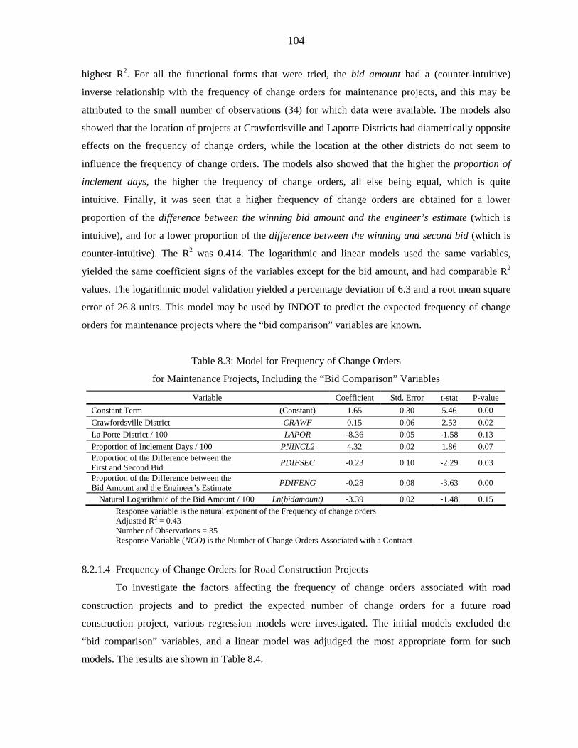
104
highest R2. For all the functional forms that were tried, the bid amount had a (counter-intuitive)
inverse relationship with the frequency of change orders for maintenance projects, and this may be
attributed to the small number of observations (34) for which data were available. The models also
showed that the location of projects at Crawfordsville and Laporte Districts had diametrically opposite
effects on the frequency of change orders, while the location at the other districts do not seem to
influence the frequency of change orders. The models also showed that the higher the proportion of
inclement days, the higher the frequency of change orders, all else being equal, which is quite
intuitive. Finally, it was seen that a higher frequency of change orders are obtained for a lower
proportion of the difference between the winning bid amount and the engineer’s estimate (which is
intuitive), and for a lower proportion of the difference between the winning and second bid (which is
counter-intuitive). The R2 was 0.414. The logarithmic and linear models used the same variables,
yielded the same coefficient signs of the variables except for the bid amount, and had comparable R2
values. The logarithmic model validation yielded a percentage deviation of 6.3 and a root mean square
error of 26.8 units. This model may be used by INDOT to predict the expected frequency of change
orders for maintenance projects where the “bid comparison” variables are known.
Table 8.3: Model for Frequency of Change Orders
for Maintenance Projects, Including the “Bid Comparison” Variables
Variable Coefficient Std. Error t-stat P-value Constant Term (Constant) 1.65 0.30 5.46 0.00 Crawfordsville District CRAWF 0.15 0.06 2.53 0.02 La Porte District / 100 LAPOR -8.36 0.05 -1.58 0.13 Proportion of Inclement Days / 100 PNINCL2 4.32 0.02 1.86 0.07 Proportion of the Difference between the First and Second Bid PDIFSEC -0.23 0.10 -2.29 0.03
Proportion of the Difference between the Bid Amount and the Engineer’s Estimate PDIFENG -0.28 0.08 -3.63 0.00
Natural Logarithmic of the Bid Amount / 100 Ln(bidamount) -3.39 0.02 -1.48 0.15 Response variable is the natural exponent of the Frequency of change orders Adjusted R2 = 0.43 Number of Observations = 35 Response Variable (NCO) is the Number of Change Orders Associated with a Contract
8.2.1.4 Frequency of Change Orders for Road Construction Projects
To investigate the factors affecting the frequency of change orders associated with road
construction projects and to predict the expected number of change orders for a future road
construction project, various regression models were investigated. The initial models excluded the
“bid comparison” variables, and a linear model was adjudged the most appropriate form for such
models. The results are shown in Table 8.4.
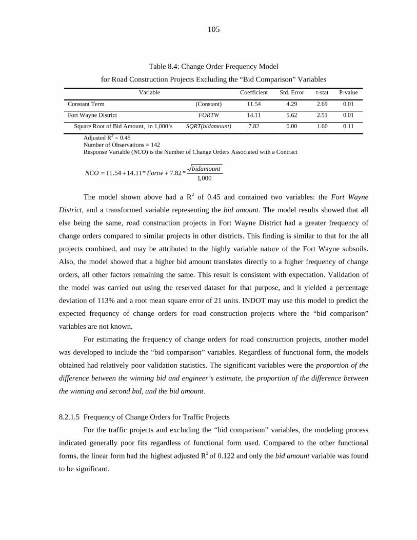
105
Table 8.4: Change Order Frequency Model
for Road Construction Projects Excluding the “Bid Comparison” Variables
Variable Coefficient Std. Error t-stat P-value
Constant Term (Constant) 11.54 4.29 2.69 0.01
Fort Wayne District FORTW 14.11 5.62 2.51 0.01
Square Root of Bid Amount, in 1,000’s SQRT(bidamount) 7.82 0.00 1.60 0.11
Adjusted R2 = 0.45 Number of Observations = 142 Response Variable (NCO) is the Number of Change Orders Associated with a Contract
000,1*82.7*11.1454.11 bidamountFortwNCO ++=
The model shown above had a R2 of 0.45 and contained two variables: the Fort Wayne
District, and a transformed variable representing the bid amount. The model results showed that all
else being the same, road construction projects in Fort Wayne District had a greater frequency of
change orders compared to similar projects in other districts. This finding is similar to that for the all
projects combined, and may be attributed to the highly variable nature of the Fort Wayne subsoils.
Also, the model showed that a higher bid amount translates directly to a higher frequency of change
orders, all other factors remaining the same. This result is consistent with expectation. Validation of
the model was carried out using the reserved dataset for that purpose, and it yielded a percentage
deviation of 113% and a root mean square error of 21 units. INDOT may use this model to predict the
expected frequency of change orders for road construction projects where the “bid comparison”
variables are not known.
For estimating the frequency of change orders for road construction projects, another model
was developed to include the “bid comparison” variables. Regardless of functional form, the models
obtained had relatively poor validation statistics. The significant variables were the proportion of the
difference between the winning bid and engineer’s estimate, the proportion of the difference between
the winning and second bid, and the bid amount.
8.2.1.5 Frequency of Change Orders for Traffic Projects
For the traffic projects and excluding the “bid comparison” variables, the modeling process
indicated generally poor fits regardless of functional form used. Compared to the other functional
forms, the linear form had the highest adjusted R2 of 0.122 and only the bid amount variable was found
to be significant.
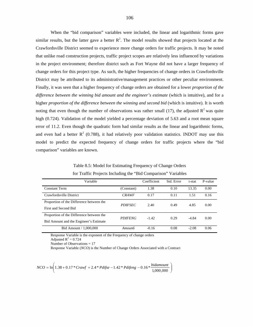
106
When the “bid comparison” variables were included, the linear and logarithmic forms gave
similar results, but the latter gave a better R2. The model results showed that projects located at the
Crawfordsville District seemed to experience more change orders for traffic projects. It may be noted
that unlike road construction projects, traffic project scopes are relatively less influenced by variations
in the project environment; therefore district such as Fort Wayne did not have a larger frequency of
change orders for this project type. As such, the higher frequencies of change orders in Crawfordsville
District may be attributed to its administrative/management practices or other peculiar environment.
Finally, it was seen that a higher frequency of change orders are obtained for a lower proportion of the
difference between the winning bid amount and the engineer’s estimate (which is intuitive), and for a
higher proportion of the difference between the winning and second bid (which is intuitive). It is worth
noting that even though the number of observations was rather small (17), the adjusted R2 was quite
high (0.724). Validation of the model yielded a percentage deviation of 5.63 and a root mean square
error of 11.2. Even though the quadratic form had similar results as the linear and logarithmic forms,
and even had a better R2 (0.788), it had relatively poor validation statistics. INDOT may use this
model to predict the expected frequency of change orders for traffic projects where the “bid
comparison” variables are known.
Table 8.5: Model for Estimating Frequency of Change Orders
for Traffic Projects Including the “Bid Comparison” Variables
Variable Coefficient Std. Error t-stat P-value
Constant Term (Constant) 1.38 0.10 13.35 0.00
Crawfordsville District CRAWF 0.17 0.11 1.51 0.16
Proportion of the Difference between the
First and Second Bid PDIFSEC 2.40 0.49 4.85 0.00
Proportion of the Difference between the
Bid Amount and the Engineer’s Estimate PDIFENG -1.42 0.29 -4.84 0.00
Bid Amount / 1,000,000 Amoun6 -0.16 0.08 -2.08 0.06
Response Variable is the exponent of the Frequency of change orders Adjusted R2 = 0.724 Number of Observations = 17 Response Variable (NCO) is the Number of Change Orders Associated with a Contract
⎟⎟⎠
⎞⎜⎜⎝
⎛−−++=
000,000,1*16.0*42.1*4.2*17.038.1ln bidamountPdifengPdifseCrawfNCO
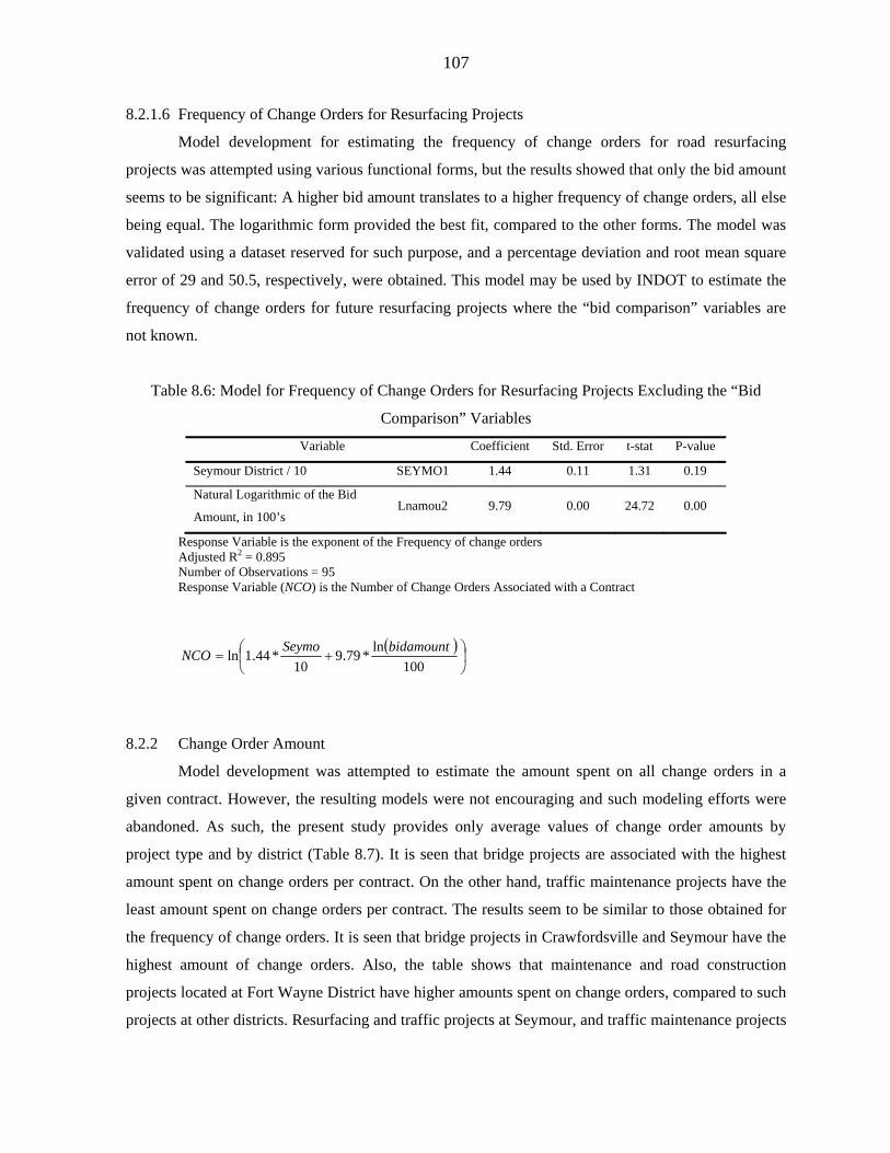
107
8.2.1.6 Frequency of Change Orders for Resurfacing Projects
Model development for estimating the frequency of change orders for road resurfacing
projects was attempted using various functional forms, but the results showed that only the bid amount
seems to be significant: A higher bid amount translates to a higher frequency of change orders, all else
being equal. The logarithmic form provided the best fit, compared to the other forms. The model was
validated using a dataset reserved for such purpose, and a percentage deviation and root mean square
error of 29 and 50.5, respectively, were obtained. This model may be used by INDOT to estimate the
frequency of change orders for future resurfacing projects where the “bid comparison” variables are
not known.
Table 8.6: Model for Frequency of Change Orders for Resurfacing Projects Excluding the “Bid
Comparison” Variables
Variable Coefficient Std. Error t-stat P-value
Seymour District / 10 SEYMO1 1.44 0.11 1.31 0.19
Natural Logarithmic of the Bid
Amount, in 100’s Lnamou2 9.79 0.00 24.72 0.00
Response Variable is the exponent of the Frequency of change orders Adjusted R2 = 0.895 Number of Observations = 95 Response Variable (NCO) is the Number of Change Orders Associated with a Contract
( )⎟⎠
⎞⎜⎝
⎛ +=100
ln*79.910
*44.1ln bidamountSeymoNCO
8.2.2 Change Order Amount
Model development was attempted to estimate the amount spent on all change orders in a
given contract. However, the resulting models were not encouraging and such modeling efforts were
abandoned. As such, the present study provides only average values of change order amounts by
project type and by district (Table 8.7). It is seen that bridge projects are associated with the highest
amount spent on change orders per contract. On the other hand, traffic maintenance projects have the
least amount spent on change orders per contract. The results seem to be similar to those obtained for
the frequency of change orders. It is seen that bridge projects in Crawfordsville and Seymour have the
highest amount of change orders. Also, the table shows that maintenance and road construction
projects located at Fort Wayne District have higher amounts spent on change orders, compared to such
projects at other districts. Resurfacing and traffic projects at Seymour, and traffic maintenance projects
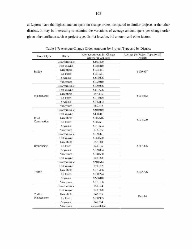
108
at Laporte have the highest amount spent on change orders, compared to similar projects at the other
districts. It may be interesting to examine the variations of average amount spent per change order
given other attributes such as project type, district location, bid amount, and other factors.
Table 8.7: Average Change Order Amounts by Project Type and by District
Project Type District Average Amount for Change Orders Per Contract
Average per Project Type, for all Districts
Crawfordsville $245,409 Fort Wayne $138,819 Greenfield $174,451 La Porte $161,581 Seymour $234,006
Bridge
Vincennes $102,010
$179,997
Crawfordsville $129,056 Fort Wayne $431,666 Greenfield $97,115 La Porte $154,079 Seymour $136,803
Maintenance
Vincennes $86,312
$164,082
Crawfordsville $210,919 Fort Wayne $308,341 Greenfield $115,616 La Porte $115,531 Seymour $181,504
Road Construction
Vincennes $72,595
$164,569
Crawfordsville $109,371 Fort Wayne $143,620 Greenfield $57,369 La Porte $41,635 Seymour $189,894
Vincennes $128,550
Resurfacing
Fort Wayne $28,583
$117,365
Crawfordsville $218,514 Fort Wayne $79,912 Greenfield $151,436 La Porte $100,274 Seymour $273,810
Traffic
Vincennes $181,156
$162,776
Crawfordsville $51,824 Fort Wayne $28,583 Greenfield $42,215 La Porte $100,965 Seymour $46,534
Traffic Maintenance
Vincennes not available
$55,669
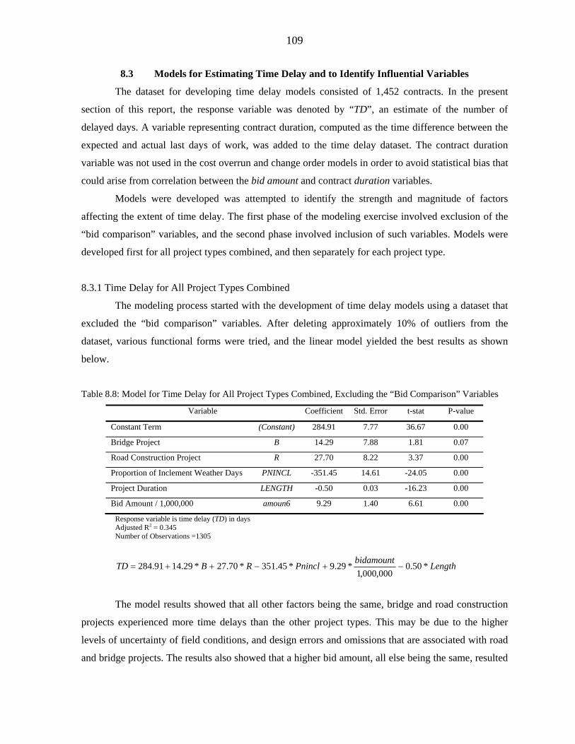
109
8.3 Models for Estimating Time Delay and to Identify Influential Variables
The dataset for developing time delay models consisted of 1,452 contracts. In the present
section of this report, the response variable was denoted by “TD”, an estimate of the number of
delayed days. A variable representing contract duration, computed as the time difference between the
expected and actual last days of work, was added to the time delay dataset. The contract duration
variable was not used in the cost overrun and change order models in order to avoid statistical bias that
could arise from correlation between the bid amount and contract duration variables.
Models were developed was attempted to identify the strength and magnitude of factors
affecting the extent of time delay. The first phase of the modeling exercise involved exclusion of the
“bid comparison” variables, and the second phase involved inclusion of such variables. Models were
developed first for all project types combined, and then separately for each project type.
8.3.1 Time Delay for All Project Types Combined
The modeling process started with the development of time delay models using a dataset that
excluded the “bid comparison” variables. After deleting approximately 10% of outliers from the
dataset, various functional forms were tried, and the linear model yielded the best results as shown
below.
Table 8.8: Model for Time Delay for All Project Types Combined, Excluding the “Bid Comparison” Variables
Variable Coefficient Std. Error t-stat P-value
Constant Term (Constant) 284.91 7.77 36.67 0.00
Bridge Project B 14.29 7.88 1.81 0.07
Road Construction Project R 27.70 8.22 3.37 0.00
Proportion of Inclement Weather Days PNINCL -351.45 14.61 -24.05 0.00
Project Duration LENGTH -0.50 0.03 -16.23 0.00
Bid Amount / 1,000,000 amoun6 9.29 1.40 6.61 0.00
Response variable is time delay (TD) in days Adjusted R2 = 0.345 Number of Observations =1305
LengthbidamountPninclRBTD *50.0
000,000,1*29.9*45.351*70.27*29.1491.284 −+−++=
The model results showed that all other factors being the same, bridge and road construction
projects experienced more time delays than the other project types. This may be due to the higher
levels of uncertainty of field conditions, and design errors and omissions that are associated with road
and bridge projects. The results also showed that a higher bid amount, all else being the same, resulted
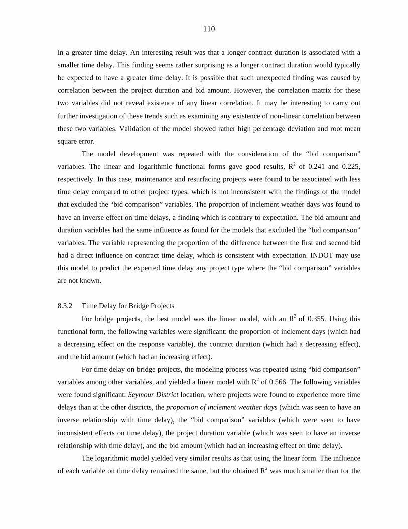
110
in a greater time delay. An interesting result was that a longer contract duration is associated with a
smaller time delay. This finding seems rather surprising as a longer contract duration would typically
be expected to have a greater time delay. It is possible that such unexpected finding was caused by
correlation between the project duration and bid amount. However, the correlation matrix for these
two variables did not reveal existence of any linear correlation. It may be interesting to carry out
further investigation of these trends such as examining any existence of non-linear correlation between
these two variables. Validation of the model showed rather high percentage deviation and root mean
square error.
The model development was repeated with the consideration of the “bid comparison”
variables. The linear and logarithmic functional forms gave good results, R2 of 0.241 and 0.225,
respectively. In this case, maintenance and resurfacing projects were found to be associated with less
time delay compared to other project types, which is not inconsistent with the findings of the model
that excluded the “bid comparison” variables. The proportion of inclement weather days was found to
have an inverse effect on time delays, a finding which is contrary to expectation. The bid amount and
duration variables had the same influence as found for the models that excluded the “bid comparison”
variables. The variable representing the proportion of the difference between the first and second bid
had a direct influence on contract time delay, which is consistent with expectation. INDOT may use
this model to predict the expected time delay any project type where the “bid comparison” variables
are not known.
8.3.2 Time Delay for Bridge Projects
For bridge projects, the best model was the linear model, with an R2 of 0.355. Using this
functional form, the following variables were significant: the proportion of inclement days (which had
a decreasing effect on the response variable), the contract duration (which had a decreasing effect),
and the bid amount (which had an increasing effect).
For time delay on bridge projects, the modeling process was repeated using “bid comparison”
variables among other variables, and yielded a linear model with R2 of 0.566. The following variables
were found significant: Seymour District location, where projects were found to experience more time
delays than at the other districts, the proportion of inclement weather days (which was seen to have an
inverse relationship with time delay), the “bid comparison” variables (which were seen to have
inconsistent effects on time delay), the project duration variable (which was seen to have an inverse
relationship with time delay), and the bid amount (which had an increasing effect on time delay).
The logarithmic model yielded very similar results as that using the linear form. The influence
of each variable on time delay remained the same, but the obtained R2 was much smaller than for the
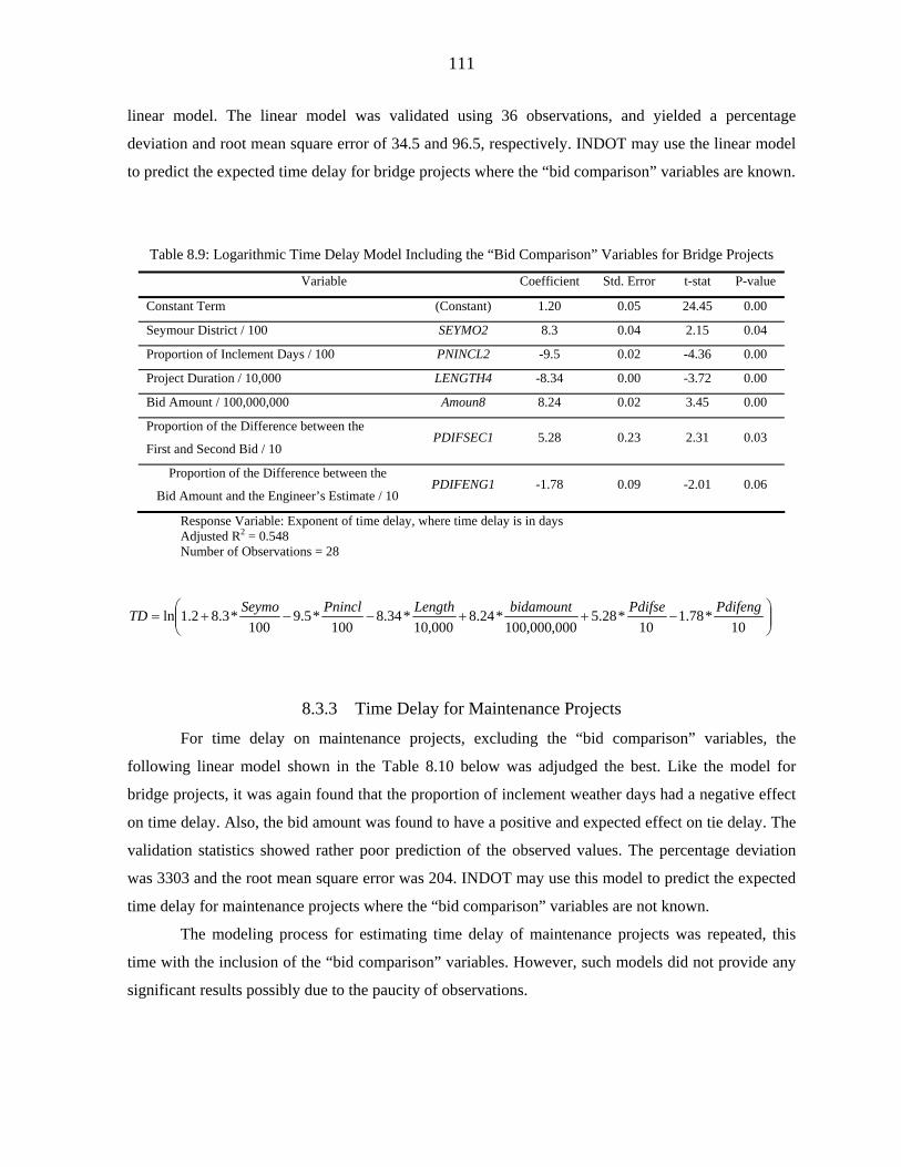
111
linear model. The linear model was validated using 36 observations, and yielded a percentage
deviation and root mean square error of 34.5 and 96.5, respectively. INDOT may use the linear model
to predict the expected time delay for bridge projects where the “bid comparison” variables are known.
Table 8.9: Logarithmic Time Delay Model Including the “Bid Comparison” Variables for Bridge Projects
Variable Coefficient Std. Error t-stat P-value
Constant Term (Constant) 1.20 0.05 24.45 0.00
Seymour District / 100 SEYMO2 8.3 0.04 2.15 0.04
Proportion of Inclement Days / 100 PNINCL2 -9.5 0.02 -4.36 0.00
Project Duration / 10,000 LENGTH4 -8.34 0.00 -3.72 0.00
Bid Amount / 100,000,000 Amoun8 8.24 0.02 3.45 0.00
Proportion of the Difference between the
First and Second Bid / 10 PDIFSEC1 5.28 0.23 2.31 0.03
Proportion of the Difference between the
Bid Amount and the Engineer’s Estimate / 10 PDIFENG1 -1.78 0.09 -2.01 0.06
Response Variable: Exponent of time delay, where time delay is in days Adjusted R2 = 0.548 Number of Observations = 28
⎟⎟⎠
⎞⎜⎜⎝
⎛−++−−+=
10*78.1
10*28.5
000,000,100*24.8
000,10*34.8
100*5.9
100*3.82.1ln PdifengPdifsebidamountLengthPninclSeymoTD
8.3.3 Time Delay for Maintenance Projects
For time delay on maintenance projects, excluding the “bid comparison” variables, the
following linear model shown in the Table 8.10 below was adjudged the best. Like the model for
bridge projects, it was again found that the proportion of inclement weather days had a negative effect
on time delay. Also, the bid amount was found to have a positive and expected effect on tie delay. The
validation statistics showed rather poor prediction of the observed values. The percentage deviation
was 3303 and the root mean square error was 204. INDOT may use this model to predict the expected
time delay for maintenance projects where the “bid comparison” variables are not known.
The modeling process for estimating time delay of maintenance projects was repeated, this
time with the inclusion of the “bid comparison” variables. However, such models did not provide any
significant results possibly due to the paucity of observations.
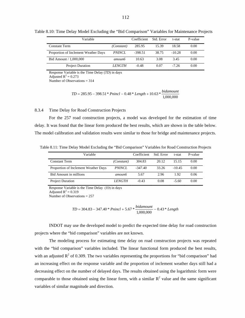
112
Table 8.10: Time Delay Model Excluding the “Bid Comparison” Variables for Maintenance Projects
Variable Coefficient Std. Error t-stat P-value
Constant Term (Constant) 285.95 15.39 18.58 0.00
Proportion of Inclement Weather Days PNINCL -398.51 38.75 -10.28 0.00
Bid Amount / 1,000,000 amoun6 10.63 3.08 3.45 0.00
Project Duration LENGTH -0.48 0.07 -7.26 0.00
Response Variable is the Time Delay (TD) in days Adjusted R2 = 0.273 Number of Observations = 314
000,000,1*63.10*48.0*51.39895.285 bidamountLengthPninclTD +−−=
8.3.4 Time Delay for Road Construction Projects
For the 257 road construction projects, a model was developed for the estimation of time
delay. It was found that the linear form produced the best results, which are shown in the table below.
The model calibration and validation results were similar to those for bridge and maintenance projects.
Table 8.11: Time Delay Model Excluding the “Bid Comparison” Variables for Road Construction Projects
Variable Coefficient Std. Error t-stat P-value
Constant Term (Constant) 304.83 20.12 15.15 0.00
Proportion of Inclement Weather Days PNINCL -347.40 33.26 -10.45 0.00
Bid Amount in millions amoun6 5.67 2.96 1.92 0.06
Project Duration LENGTH -0.43 0.08 -5.60 0.00
Response Variable is the Time Delay (TD) in days Adjusted R2 = 0.319 Number of Observations = 257
LengthbidamountPninclTD *43.0
000,000,1*67.5*40.34783.304 −+−=
INDOT may use the developed model to predict the expected time delay for road construction
projects where the “bid comparison” variables are not known.
The modeling process for estimating time delay on road construction projects was repeated
with the “bid comparison” variables included. The linear functional form produced the best results,
with an adjusted R2 of 0.309. The two variables representing the proportions for “bid comparison” had
an increasing effect on the response variable and the proportion of inclement weather days still had a
decreasing effect on the number of delayed days. The results obtained using the logarithmic form were
comparable to those obtained using the linear form, with a similar R2 value and the same significant
variables of similar magnitude and direction.
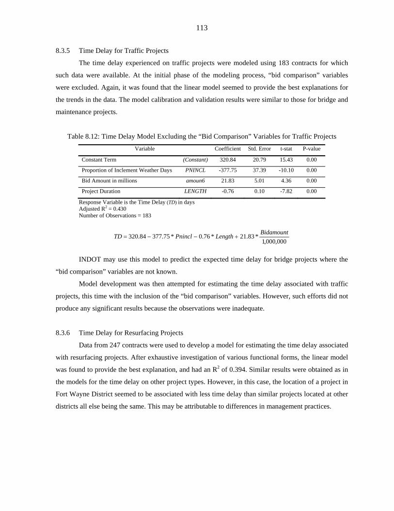
113
8.3.5 Time Delay for Traffic Projects
The time delay experienced on traffic projects were modeled using 183 contracts for which
such data were available. At the initial phase of the modeling process, “bid comparison” variables
were excluded. Again, it was found that the linear model seemed to provide the best explanations for
the trends in the data. The model calibration and validation results were similar to those for bridge and
maintenance projects.
Table 8.12: Time Delay Model Excluding the “Bid Comparison” Variables for Traffic Projects
Variable Coefficient Std. Error t-stat P-value
Constant Term (Constant) 320.84 20.79 15.43 0.00
Proportion of Inclement Weather Days PNINCL -377.75 37.39 -10.10 0.00
Bid Amount in millions amoun6 21.83 5.01 4.36 0.00
Project Duration LENGTH -0.76 0.10 -7.82 0.00
Response Variable is the Time Delay (TD) in days Adjusted R2 = 0.430 Number of Observations = 183
000,000,1*83.21*76.0*75.37784.320 BidamountLengthPninclTD +−−=
INDOT may use this model to predict the expected time delay for bridge projects where the
“bid comparison” variables are not known.
Model development was then attempted for estimating the time delay associated with traffic
projects, this time with the inclusion of the “bid comparison” variables. However, such efforts did not
produce any significant results because the observations were inadequate.
8.3.6 Time Delay for Resurfacing Projects
Data from 247 contracts were used to develop a model for estimating the time delay associated
with resurfacing projects. After exhaustive investigation of various functional forms, the linear model
was found to provide the best explanation, and had an R2 of 0.394. Similar results were obtained as in
the models for the time delay on other project types. However, in this case, the location of a project in
Fort Wayne District seemed to be associated with less time delay than similar projects located at other
districts all else being the same. This may be attributable to differences in management practices.
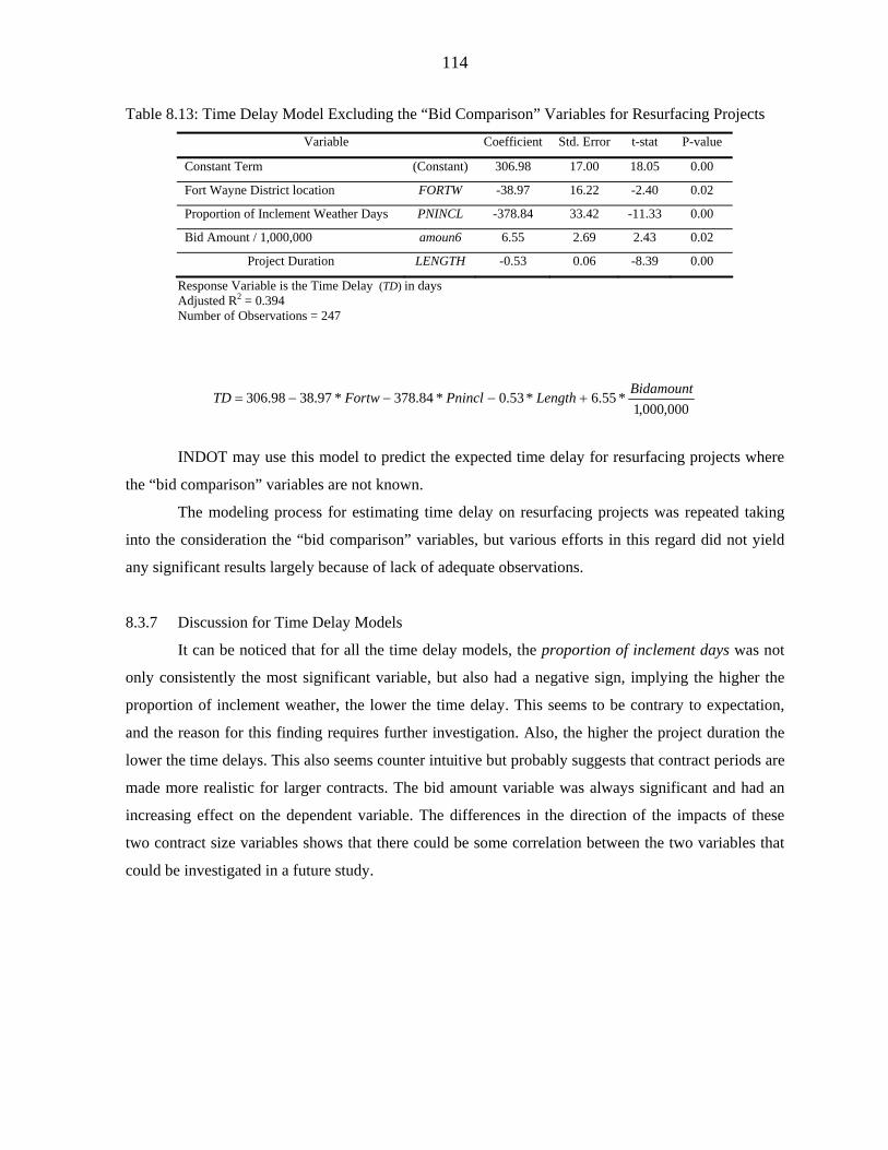
114
Table 8.13: Time Delay Model Excluding the “Bid Comparison” Variables for Resurfacing Projects
Variable Coefficient Std. Error t-stat P-value
Constant Term (Constant) 306.98 17.00 18.05 0.00
Fort Wayne District location FORTW -38.97 16.22 -2.40 0.02
Proportion of Inclement Weather Days PNINCL -378.84 33.42 -11.33 0.00
Bid Amount / 1,000,000 amoun6 6.55 2.69 2.43 0.02
Project Duration LENGTH -0.53 0.06 -8.39 0.00
Response Variable is the Time Delay (TD) in days Adjusted R2 = 0.394 Number of Observations = 247
000,000,1*55.6*53.0*84.378*97.3898.306 BidamountLengthPninclFortwTD +−−−=
INDOT may use this model to predict the expected time delay for resurfacing projects where
the “bid comparison” variables are not known.
The modeling process for estimating time delay on resurfacing projects was repeated taking
into the consideration the “bid comparison” variables, but various efforts in this regard did not yield
any significant results largely because of lack of adequate observations.
8.3.7 Discussion for Time Delay Models
It can be noticed that for all the time delay models, the proportion of inclement days was not
only consistently the most significant variable, but also had a negative sign, implying the higher the
proportion of inclement weather, the lower the time delay. This seems to be contrary to expectation,
and the reason for this finding requires further investigation. Also, the higher the project duration the
lower the time delays. This also seems counter intuitive but probably suggests that contract periods are
made more realistic for larger contracts. The bid amount variable was always significant and had an
increasing effect on the dependent variable. The differences in the direction of the impacts of these
two contract size variables shows that there could be some correlation between the two variables that
could be investigated in a future study.
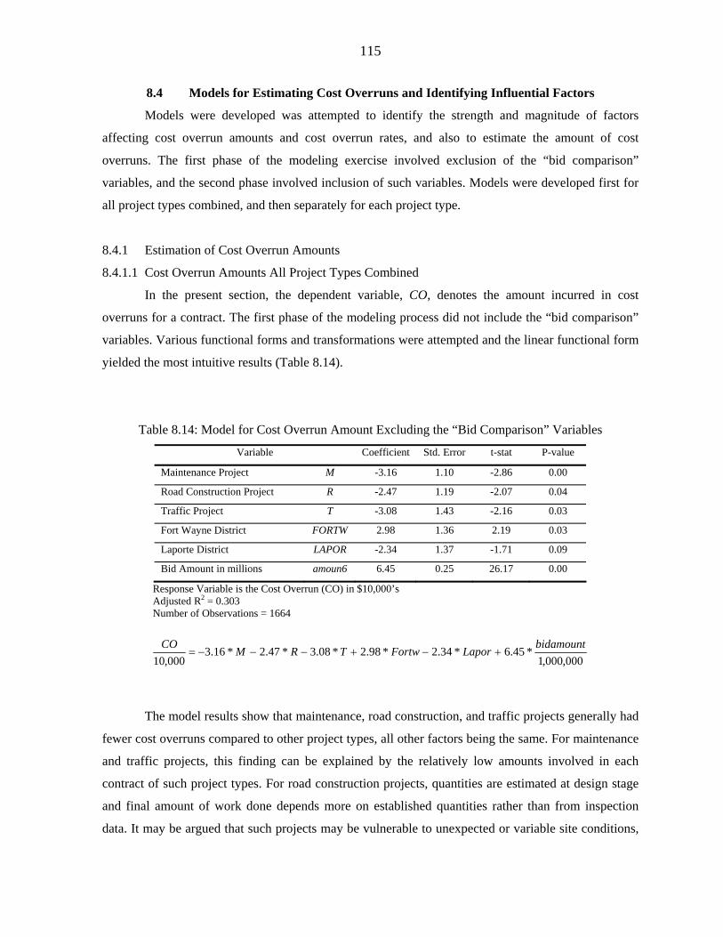
115
8.4 Models for Estimating Cost Overruns and Identifying Influential Factors
Models were developed was attempted to identify the strength and magnitude of factors
affecting cost overrun amounts and cost overrun rates, and also to estimate the amount of cost
overruns. The first phase of the modeling exercise involved exclusion of the “bid comparison”
variables, and the second phase involved inclusion of such variables. Models were developed first for
all project types combined, and then separately for each project type.
8.4.1 Estimation of Cost Overrun Amounts
8.4.1.1 Cost Overrun Amounts All Project Types Combined
In the present section, the dependent variable, CO, denotes the amount incurred in cost
overruns for a contract. The first phase of the modeling process did not include the “bid comparison”
variables. Various functional forms and transformations were attempted and the linear functional form
yielded the most intuitive results (Table 8.14).
Table 8.14: Model for Cost Overrun Amount Excluding the “Bid Comparison” Variables
Variable Coefficient Std. Error t-stat P-value
Maintenance Project M -3.16 1.10 -2.86 0.00
Road Construction Project R -2.47 1.19 -2.07 0.04
Traffic Project T -3.08 1.43 -2.16 0.03
Fort Wayne District FORTW 2.98 1.36 2.19 0.03
Laporte District LAPOR -2.34 1.37 -1.71 0.09
Bid Amount in millions amoun6 6.45 0.25 26.17 0.00
Response Variable is the Cost Overrun (CO) in $10,000’s Adjusted R2 = 0.303 Number of Observations = 1664
000,000,1*45.6*34.2*98.2*08.3*47.2*16.3
000,10bidamountLaporFortwTRMCO
+−+−−−=
The model results show that maintenance, road construction, and traffic projects generally had
fewer cost overruns compared to other project types, all other factors being the same. For maintenance
and traffic projects, this finding can be explained by the relatively low amounts involved in each
contract of such project types. For road construction projects, quantities are estimated at design stage
and final amount of work done depends more on established quantities rather than from inspection
data. It may be argued that such projects may be vulnerable to unexpected or variable site conditions,
116
thus making such projects have high overruns. The sign obtained therefore appears to be a net effect of
these two contrasting justifications. Besides, the variable representing district which was found
significant, may account partly for the relationship between high cost overruns and site variability. The
model showed that a project located at Fort Wayne District is associated with more cost overruns
compared to other districts, all else being equal. Also, the model showed that projects located at
Laporte District is associated with lower cost overruns compared to other districts, all other factors
being the same. It was found that the bid amount variable was the most significant, and that a higher
bid amount translates to a higher amount of cost overruns, all else being equal. The proportion of
inclement weather days was not found to be significant. Validation of the models yielded rather high
values of percentage deviation (5814) and root mean square error ($309,000). INDOT may use the
developed model to predict the expected cost overrun for any project type where the “bid comparison”
variables are not known.
The model development was also carried out to include the “bid comparison” variables. Of the
several forms investigated, only the logarithmic form produced encouraging results, with an R2 of
0.23. The model showed that traffic maintenance projects generally had more cost overruns than other
project types, all else being the same. Also, it was found that a higher level of competition was
associated with a greater amount of cost overruns. This may be attributed to the fact that in a
competitive environment, contractors try to reduce their prices as much as possible, but such
reductions may result in unrealistic bid prices. Finally, the model with the “bid comparison” variables
showed that a higher bid amount had an increasing effect on cost overruns. INDOT may use this
model to predict the expected cost overrun amount for any project type where the “bid comparison”
variables are known.
8.4.1.2 Cost Overrun Amounts for Bridge Projects
Using the 449 bridge contracts, models were developed to estimate the amount of cost
overruns for bridge projects. The first step was to exclude the “bid comparison” variables. The linear
model was found to be the most intuitive and gave the best results. From the model results, it is
suggested that bridge projects located at Laporte District experienced fewer cost overruns than those
located at other districts, all other factors being the same. Also, the bid amount had an increasing
effect on cost overrun amount. This model may be used by INDOT to predict the expected cost
overrun for bridge projects where the “bid comparison” variables are unknown.
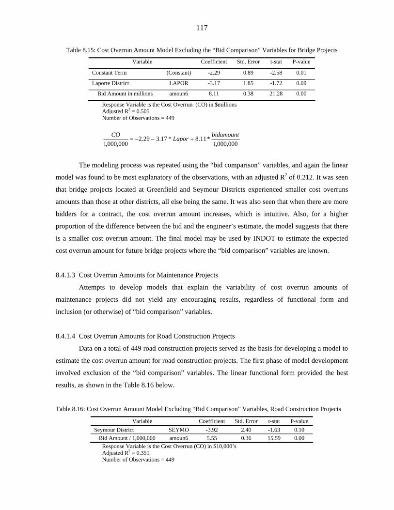
117
Table 8.15: Cost Overrun Amount Model Excluding the “Bid Comparison” Variables for Bridge Projects
Variable Coefficient Std. Error t-stat P-value
Constant Term (Constant) -2.29 0.89 -2.58 0.01
Laporte District LAPOR -3.17 1.85 -1.72 0.09
Bid Amount in millions amoun6 8.11 0.38 21.28 0.00
Response Variable is the Cost Overrun (CO) in $millions Adjusted R2 = 0.505 Number of Observations = 449
000,000,1*11.8*17.329.2
000,000,1bidamountLaporCO
+−−=
The modeling process was repeated using the “bid comparison” variables, and again the linear
model was found to be most explanatory of the observations, with an adjusted R2 of 0.212. It was seen
that bridge projects located at Greenfield and Seymour Districts experienced smaller cost overruns
amounts than those at other districts, all else being the same. It was also seen that when there are more
bidders for a contract, the cost overrun amount increases, which is intuitive. Also, for a higher
proportion of the difference between the bid and the engineer’s estimate, the model suggests that there
is a smaller cost overrun amount. The final model may be used by INDOT to estimate the expected
cost overrun amount for future bridge projects where the “bid comparison” variables are known.
8.4.1.3 Cost Overrun Amounts for Maintenance Projects
Attempts to develop models that explain the variability of cost overrun amounts of
maintenance projects did not yield any encouraging results, regardless of functional form and
inclusion (or otherwise) of “bid comparison” variables.
8.4.1.4 Cost Overrun Amounts for Road Construction Projects
Data on a total of 449 road construction projects served as the basis for developing a model to
estimate the cost overrun amount for road construction projects. The first phase of model development
involved exclusion of the “bid comparison” variables. The linear functional form provided the best
results, as shown in the Table 8.16 below.
Table 8.16: Cost Overrun Amount Model Excluding “Bid Comparison” Variables, Road Construction Projects
Variable Coefficient Std. Error t-stat P-value Seymour District SEYMO -3.92 2.40 -1.63 0.10
Bid Amount / 1,000,000 amoun6 5.55 0.36 15.59 0.00 Response Variable is the Cost Overrun (CO) in $10,000’s Adjusted R2 = 0.351 Number of Observations = 449
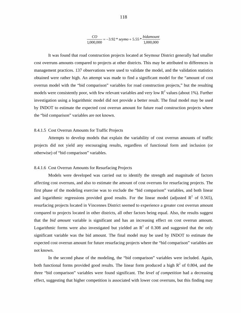
118
000,000,1*55.5*92.3
000,000,1bidamountseymoCO
+−=
It was found that road construction projects located at Seymour District generally had smaller
cost overruns amounts compared to projects at other districts. This may be attributed to differences in
management practices. 137 observations were used to validate the model, and the validation statistics
obtained were rather high. An attempt was made to find a significant model for the “amount of cost
overrun model with the “bid comparison” variables for road construction projects,” but the resulting
models were consistently poor, with few relevant variables and very low R2 values (about 1%). Further
investigation using a logarithmic model did not provide a better result. The final model may be used
by INDOT to estimate the expected cost overrun amount for future road construction projects where
the “bid comparison” variables are not known.
8.4.1.5 Cost Overrun Amounts for Traffic Projects
Attempts to develop models that explain the variability of cost overrun amounts of traffic
projects did not yield any encouraging results, regardless of functional form and inclusion (or
otherwise) of “bid comparison” variables.
8.4.1.6 Cost Overrun Amounts for Resurfacing Projects
Models were developed was carried out to identify the strength and magnitude of factors
affecting cost overruns, and also to estimate the amount of cost overruns for resurfacing projects. The
first phase of the modeling exercise was to exclude the “bid comparison” variables, and both linear
and logarithmic regressions provided good results. For the linear model (adjusted R2 of 0.565),
resurfacing projects located in Vincennes District seemed to experience a greater cost overrun amount
compared to projects located in other districts, all other factors being equal. Also, the results suggest
that the bid amount variable is significant and has an increasing effect on cost overrun amount.
Logarithmic forms were also investigated but yielded an R2 of 0.308 and suggested that the only
significant variable was the bid amount. The final model may be used by INDOT to estimate the
expected cost overrun amount for future resurfacing projects where the “bid comparison” variables are
not known.
In the second phase of the modeling, the “bid comparison” variables were included. Again,
both functional forms provided good results. The linear form produced a high R2 of 0.804, and the
three “bid comparison” variables were found significant. The level of competition had a decreasing
effect, suggesting that higher competition is associated with lower cost overruns, but this finding may
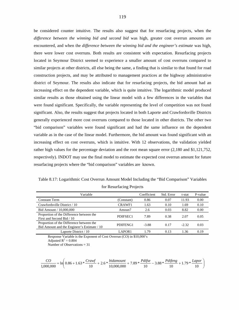
119
be considered counter intuitive. The results also suggest that for resurfacing projects, when the
difference between the winning bid and second bid was high, greater cost overrun amounts are
encountered, and when the difference between the winning bid and the engineer’s estimate was high,
there were lower cost overruns. Both results are consistent with expectation. Resurfacing projects
located in Seymour District seemed to experience a smaller amount of cost overruns compared to
similar projects at other districts, all else being the same, a finding that is similar to that found for road
construction projects, and may be attributed to management practices at the highway administrative
district of Seymour. The results also indicate that for resurfacing projects, the bid amount had an
increasing effect on the dependent variable, which is quite intuitive. The logarithmic model produced
similar results as those obtained using the linear model with a few differences in the variables that
were found significant. Specifically, the variable representing the level of competition was not found
significant. Also, the results suggest that projects located in both Laporte and Crawfordsville Districts
generally experienced more cost overruns compared to those located in other districts. The other two
“bid comparison” variables were found significant and had the same influence on the dependent
variable as in the case of the linear model. Furthermore, the bid amount was found significant with an
increasing effect on cost overruns, which is intuitive. With 12 observations, the validation yielded
rather high values for the percentage deviation and the root mean square error (2,180 and $1,121,752,
respectively). INDOT may use the final model to estimate the expected cost overrun amount for future
resurfacing projects where the “bid comparison” variables are known.
Table 8.17: Logarithmic Cost Overrun Amount Model Including the “Bid Comparison” Variables
for Resurfacing Projects
Variable Coefficient Std. Error t-stat P-value Constant Term (Constant) 0.86 0.07 11.93 0.00 Crawfordsville District / 10 CRAWF1 1.63 0.10 1.69 0.10 Bid Amount / 10,000,000 Amoun7 2.6 0.03 8.82 0.00 Proportion of the Difference between the First and Second Bid / 10 PDIFSEC1 7.89 0.38 2.07 0.05
Proportion of the Difference between the Bid Amount and the Engineer’s Estimate / 10 PDIFENG1 -3.88 0.17 -2.32 0.03
Laporte District / 10 LAPOR1 1.79 0.13 1.36 0.19 Response Variable is the Exponent of Cost Overrun (CO) in $10,000’s Adjusted R2 = 0.804 Number of Observations = 31
⎟⎟⎠
⎞⎜⎜⎝
⎛+−+++=
10*79.1
10*88.3
10*89.7
000,000,10*6.2
10*63.186.0ln
000,000,1LaporPdifengPdifsebidamountCrawfCO
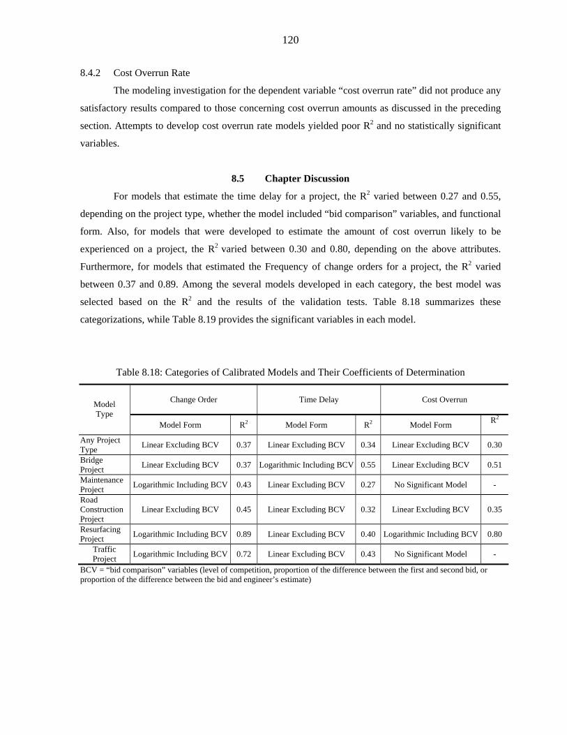
120
8.4.2 Cost Overrun Rate
The modeling investigation for the dependent variable “cost overrun rate” did not produce any
satisfactory results compared to those concerning cost overrun amounts as discussed in the preceding
section. Attempts to develop cost overrun rate models yielded poor R2 and no statistically significant
variables.
8.5 Chapter Discussion
For models that estimate the time delay for a project, the R2 varied between 0.27 and 0.55,
depending on the project type, whether the model included “bid comparison” variables, and functional
form. Also, for models that were developed to estimate the amount of cost overrun likely to be
experienced on a project, the R2 varied between 0.30 and 0.80, depending on the above attributes.
Furthermore, for models that estimated the Frequency of change orders for a project, the R2 varied
between 0.37 and 0.89. Among the several models developed in each category, the best model was
selected based on the R2 and the results of the validation tests. Table 8.18 summarizes these
categorizations, while Table 8.19 provides the significant variables in each model.
Table 8.18: Categories of Calibrated Models and Their Coefficients of Determination
Change Order Time Delay
Cost Overrun Model
Type Model Form R2 Model Form R2 Model Form R2
Any Project Type Linear Excluding BCV 0.37 Linear Excluding BCV 0.34 Linear Excluding BCV 0.30
Bridge Project Linear Excluding BCV 0.37 Logarithmic Including BCV 0.55 Linear Excluding BCV 0.51
Maintenance Project Logarithmic Including BCV 0.43 Linear Excluding BCV 0.27 No Significant Model -
Road Construction Project
Linear Excluding BCV 0.45 Linear Excluding BCV 0.32 Linear Excluding BCV 0.35
Resurfacing Project Logarithmic Including BCV 0.89 Linear Excluding BCV 0.40 Logarithmic Including BCV 0.80
Traffic Project Logarithmic Including BCV 0.72 Linear Excluding BCV 0.43 No Significant Model -
BCV = “bid comparison” variables (level of competition, proportion of the difference between the first and second bid, or proportion of the difference between the bid and engineer’s estimate)
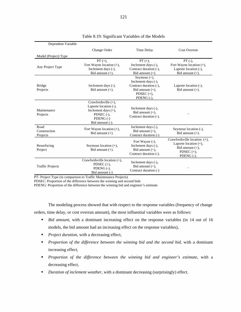
121
Table 8.19: Significant Variables of the Models
Dependent Variable Model (Project) Type
Change Order Time Delay
Cost Overrun
Any Project Type
PT (+), Fort Wayne location (+),
Inclement days (-), Bid amount (+).
PT (+), Inclement days (-),
Contract duration (-), Bid amount (+).
PT (-), Fort Wayne location (+),
Laporte location (-), Bid amount (+).
Bridge Projects
Inclement days (-), Bid amount (+).
Seymour (+), Inclement days (-),
Contract duration (-), Bid amount (+),
PDSEC (+), PDENG (-),
Laporte location (-), Bid amount (+).
Maintenance Projects
Crawfordsville (+), Laporte location (-), Inclement days (+),
PDSEC (-), PDENG (-)
Bid amount (-).
Inclement days (-), Bid amount (+),
Contract duration (-). _
Road Construction Projects
Fort Wayne location (+), Bid amount (+).
Inclement days (-), Bid amount (+),
Contract duration (-)
Seymour location (-), Bid amount (+).
Resurfacing Project
Seymour location (+), Bid amount (+).
Fort Wayne (-), Inclement days (-),
Bid amount (+), Contract duration (-).
Crawfordsville location (+), Laporte location (+),
Bid amount (+), PDSEC (+), PDENG (-).
Traffic Projects
Crawfordsville location (+), PDSEC (+), PDENG (-),
Bid amount (-)
Inclement days (-), Bid amount (+),
Contract duration (-) _
PT- Project Type (in comparison to Traffic Maintenance Projects) PDSEC: Proportion of the difference between the winning and second bids PDENG: Proportion of the difference between the winning bid and engineer’s estimate
The modeling process showed that with respect to the response variables (frequency of change
orders, time delay, or cost overrun amount), the most influential variables were as follows:
Bid amount, with a dominant increasing effect on the response variables (in 14 out of 16
models, the bid amount had an increasing effect on the response variables),
Project duration, with a decreasing effect,
Proportion of the difference between the winning bid and the second bid, with a dominant
increasing effect,
Proportion of the difference between the winning bid and engineer’s estimate, with a
decreasing effect,
Duration of inclement weather, with a dominant decreasing (surprisingly) effect.
122
8.6 Chapter Summary
This chapter provided the results of the modeling process and attempted to explain the results
found therein. A few models had satisfactory R2 and validation statistics. The results obtained were
generally consistent with expectation. However, there were a few cases where the variable signs were
counter intuitive and may need further investigation. Using the model results it may be possible to
obtain estimates of the Frequency of change orders, time delay or cost overruns associated with any
future INDOT project, given basic characteristics such as bid amount, project type, location by district,
nature of weather, and “bid comparison” variables if available.
123
CHAPTER 9 - CONCLUSIONS
This study analyzed the problem of cost overruns, time delays, and change orders associated
with INDOT projects. This was carried out using a variety of methods including an agency survey,
literature review, and statistical analyses.
The agency survey revealed that INDOT’s contract management performance in terms of cost
overruns and time delays is generally similar to that of other state DOTs. Nevertheless, cost overruns
and time delays in Indiana represent a sizeable portion of agency costs, and even a marginal reduction
can lead to substantial savings.
The study showed that between the years 1996 and 2001, 55% of all Indiana DOT contracts
experienced cost overruns, and the overall cost overrun rate was 4.5% of the bid amount. With regard
to cost overruns, it was determined that the average cost overrun amount and rate differ by project
type. Also, the strength of influential factors differ by project type The average cost overrun rates were
as follows: bridge projects -- 8.1%, road construction -- 5.6%, road resurfacing -- 2.6%, traffic projects
-- 5.6%, maintenance projects -- 7.5%. It was also determined that influential factors of cost overrun of
highway contracts include the contract bid amount, difference between the winning bid and second
bid, difference between the winning bid and the engineer’s estimate, project type and location by
district. The developed models may be used to estimate the extent of future cost overruns on the basis
of contract and project characteristics, and are therefore useful in long term budgeting and needs
assessment studies. With regard to time delay, it was also found that 12% of all INDOT contracts
experience time delays, and the average delay per contract was 115 days. The study also determined
average time delay for each type of contract. From the various statistical analyses, it was determined
that factors influential to time delays are contract bid amount, difference between the winning bid and
second bid, difference between the winning bid and the engineer’s estimate, project type and location
by district. Based on the results of the analysis, recommendations can be made for improving the
management of projects and the administration of contracts in order to reduce time delays.
Using an array of statistical methods, the present research project explored the problem
statement further. The magnitude of cost overrun, time delay and change order problems associated
INDOT’s construction projects were explored by investigating the relationships between these
parameters and key characteristics of the bidding process, project, and environment. The descriptive
124
statistics showed that the following change order types were the most critical in terms of frequency
and cost: “errors and omissions, design related,” “errors and omissions, quantity related,”
“constructability, construction related,” “constructability, design related,” and “changed field
conditions, construction related.” It was found that most of such change order reason categories were
the responsibility of INDOT or its consultants, and therefore is within INDOT’s capability to reduce
the incidence of such change orders by improving its contract management system. The descriptive
statistics also indicated that cost overruns and time delays have been on the decrease since 1997. It
was indicated that more time delays were experienced for maintenance projects compared to other
project types, and for projects in the Seymour District compared to those located at other districts. The
results of such preliminary analyses also suggested that higher cost overrun amounts were experienced
for resurfacing projects compared to other project types, and also for projects located in the Fort
Wayne District compared to other districts. Furthermore, the descriptive statistics suggested that a
higher number of change orders is associated with road construction projects compared to other
project types, and also for projects in the Greenfield District compared to other districts. The
correlation matrix analysis showed that the selected independent variables were not affected by the
problem of linear correlation, with the exception of the variables representing the “proportion of the
difference between the winning and second bids” and the “proportion of the difference between the
winning bid and the engineer’s estimate.” From the analysis of variance, it was observed that there
generally exists a statistical difference between the mean responses (cost overruns, time delays, and
change orders) of any two categories of the independent variables. The pairwise t-tests provided
confirmation of the ANOVA findings.
The last statistical method used was regression modeling to confirm the influence of the
independent variables, and to estimate values of cost overruns, time delay and change orders for future
projects. Given the inconsistent performance of a few of the developed models in terms of R2 and
validation statistics, it may be stated that some of models may be used for prediction only with
caution. The developed models provided interesting information about the factors that affect cost
overruns, time delays, and change orders. It was found that significant variables included bid amount,
project type, location by district, weather, and bid comparison variables. The level of competition was
generally found not influential. Specifically, the proportion of the difference between the winning and
second bid had a dominant increasing effect. The proportion of the difference between the winning bid
and the engineer’s estimates had a decreasing effect. These conclusions are similar to those found
from the literature review. The advantage of the present study compared to the studies found in the
literature is the greater dataset size so the resulting analysis is expected to yield results that are more
consistent.
125
A major problem encountered during the course of the present study was existence of several
change orders for which no reason was assigned to change orders. For approximately a third of all
change orders (representing one-half of amounts incurred on change orders), no reason was assigned
in the dataset. This suggests that there are a few lapses in the current management of change orders at
INDOT. The constructability reviews report from the Constructability Process Review Committee
shows that a key need was the development of a process to determine the causes of change orders.
Therefore, the tracking for change orders and their causes may be expected to improve after
implementation of such a mechanism. This recommendation was implemented on April 11, 1997.
However, examination of the change order reason database even after that date showed that most of
the “no-reason” change orders were for years subsequent to such implementation (i.e., 1999, 2000, and
2001). It is conceivable that because the year indicated in the dataset represented the final year of
work, such contracts may have started several years earlier, at which time the Constructability Process
Review Committee recommendations had not yet been implemented. Upon further investigation of
archival data, it was determined that some change orders currently categorized as having “no recorded
reason” in the dataset were actually categorized as “errors and omissions” change orders in the
archives. However, it could not be ascertained why such reasons were not transferred from the
archives to the dataset. It is obvious that further work needs to be done to identify the source and
nature of this problem.
The implementation of SiteManager will provide a more effective way to classify and code
change order information. This should reduce the occurrence of “no recorded reason” change orders
and thereby improve the accessibility and evaluation of this type of data. Since the completion of
data analysis, System Technology has deployed BAMS Decision Support System (DSS). DSS
provides an easier way to retrieve project data.
The results of the present study provided a framework for subsequent recommendations made
with a view to reducing the frequency and amounts involved in change orders, cost overruns, and time
delays at INDOT.
126
CHAPTER 10 - RECOMENDATIONS
The present study revealed some areas where it is possible to improve, and the following
recommendations are offered for consideration.
Improvements could be made to the current design review process of a project, particularly for
large, high-value projects. The study found that “design errors and omissions” was the most frequent
change order category that created the most cost. This was discussed at a November 20, 2003 meeting
attended by INDOT personnel from Budget, Operations Support, and Design. Several options were
floated such as: hiring additional design personnel to review contract documents; establishing a
review of consultant’s performance in regards to number and type of change orders occurring on
projects; and, adding additional review requirements for consultants. After much discussion the
following recommendations were made. First, a Change Order Management process needs to be
developed and implemented. This will consist of:
1. Developing a Change Order mindset in the Department.
2. Developing procedures and instructions for recording change order information in
SiteManager.
3. Developing a system of controls that routes change order information to the appropriate
personnel in Operations Support and Design Divisions.
The change order mindset would raise the necessary awareness of the problem, help develop
an agency-wide attitude geared towards the reduction of change orders, and help identify
improvements needed at various stages of the project life-cycle for mitigating the problem.
In the past, change orders have not been recorded until the end of the contract. SiteManager
allows for the recording of change order information as the project progresses. Also, with the current
INDOT change order classification code, it is often not possible to determine the appropriate code that
is applicable to all situations. The presence of so many “no indicated reason” change orders suggests
that there may be some lapses in the recording of appropriate reasons for change orders. The code may
therefore need review and modification. A system of instructions and more definitive definitions can
improve documentation and eliminate the assignment of “no indicated reason” to change orders.
The problem of change orders needs to be addressed at source. Most bidding documents (with
the exception of those for resurfacing projects) are prepared by consultants A standard report for each
consultant and for each contract could be prepared and provided to such consultants to point out errors
127
committed and how such errors may be avoided in future. Moreover, “real time” recording of change
orders would probably accelerate the process of feedback to designers and field personnel. If data
about change orders is collected on a daily basis, it is possible to create a “weekly change order report”
and route it to the appropriate personnel.
It is recommended that INDOT should design an annual report that reviews the performance
of consultants. Such a report would assign “grades” to each consultant, taking into account the number
and dollar amount of preventable change orders that are attributable to the consultant. If grades are to
be assigned in such manner, INDOT’s change order classification may be adapted to this new
objective in order to better distinguish the responsibilities of each change order type.
INDOT personnel should be given ample opportunity to carry out a detailed review of change
orders reports and their implications. Also, such personnel should be encouraged to continually
improve their methods. Obviously, implementing additional requirements will be a challenge, given
the current staffing levels and work loads at INDOT. However, an electronic routing system that
collects and distributes change order information would reduce the resources needed to implement this
recommendation.
Finally, it is recommended to develop a system that would facilitate communication of
updated information concerning cost overruns, time delays, and change orders, to the general public.
As has been done in some states (ADOT, 2003) and illustrated in Appendix G, this could be
implemented using an electronic tool that could be made available on the internet.
128
CHAPTER 11 - IMPLEMENTATION
The project constitutes an evaluation of the problem of cost overruns, time delays, and change
orders at INDOT. This research effort is consistent with INDOT’s strategic objectives for resource
management (INDOT, 2003) which include reduction in INDOT overhead costs and increase in the
efficiency of the capital program expenditures. The present study provided some initial answers to
address problems in the present system. Using the results herein as a starting point, it is possible to
carry out future work such as the implementation of a methodology to enhance contract management
at INDOT. Another activity is to develop an evaluation method or system to manage the collection,
analysis, and presentation of change orders, cost overruns, and time delays information in an efficient
manner. At the present time, there are indications that INDOT is considering establishing a new
system to record change orders online directly from the construction site. The next step would be to
develop or enhance the organization of a change order database to facilitate analysis of change order
information and preparation of periodic consultant performance reports. Furthermore, with such
enhanced information system, it will be possible to carry out future work geared towards improving
the predictive ability of models relating to change orders, time delays, and cost overruns. Finally,
conducting a meticulous review of construction management techniques used can help identify any
weaknesses in the design and construction process, thus making it possible to make more precise
recommendations for improvements in contract management at INDOT.
131
Appendix A:
Copy of E-Mail Message Soliciting Cost Overrun, Time Delay and Change Order
Information form State Highway Agencies
The Indiana Department of Transportation (INDOT) is conducting an analysis about cost overruns and time delays of its projects for the last 5 years. The analysis will look at the causes by investigating final contract information. We would like to know the extent of this problem in other DOTs. We are looking for the following information: % of contracts with time and cost overruns, average cost overrun, annual amount spent on overruns, and causes of these overruns. If you posses this information and are willing to share it with us, please forward it to (Bob McCullouch, the study supervisor) at Purdue University at [email protected]. T would be appreciated if you could please respond by December 1. Thank you in advance for your assistance.
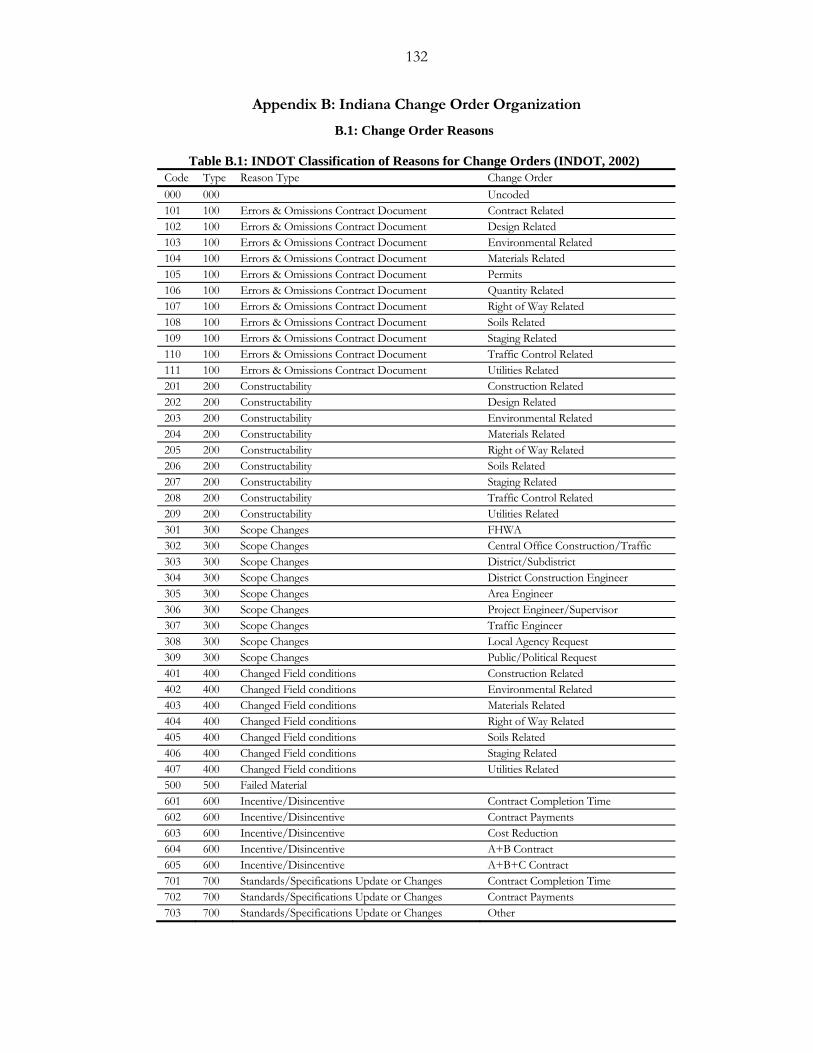
132
Appendix B: Indiana Change Order Organization
B.1: Change Order Reasons
Table B.1: INDOT Classification of Reasons for Change Orders (INDOT, 2002) Code Type Reason Type Change Order 000 000 Uncoded 101 100 Errors & Omissions Contract Document Contract Related 102 100 Errors & Omissions Contract Document Design Related 103 100 Errors & Omissions Contract Document Environmental Related 104 100 Errors & Omissions Contract Document Materials Related 105 100 Errors & Omissions Contract Document Permits 106 100 Errors & Omissions Contract Document Quantity Related 107 100 Errors & Omissions Contract Document Right of Way Related 108 100 Errors & Omissions Contract Document Soils Related 109 100 Errors & Omissions Contract Document Staging Related 110 100 Errors & Omissions Contract Document Traffic Control Related 111 100 Errors & Omissions Contract Document Utilities Related 201 200 Constructability Construction Related 202 200 Constructability Design Related 203 200 Constructability Environmental Related 204 200 Constructability Materials Related 205 200 Constructability Right of Way Related 206 200 Constructability Soils Related 207 200 Constructability Staging Related 208 200 Constructability Traffic Control Related 209 200 Constructability Utilities Related 301 300 Scope Changes FHWA 302 300 Scope Changes Central Office Construction/Traffic 303 300 Scope Changes District/Subdistrict 304 300 Scope Changes District Construction Engineer 305 300 Scope Changes Area Engineer 306 300 Scope Changes Project Engineer/Supervisor 307 300 Scope Changes Traffic Engineer 308 300 Scope Changes Local Agency Request 309 300 Scope Changes Public/Political Request 401 400 Changed Field conditions Construction Related 402 400 Changed Field conditions Environmental Related 403 400 Changed Field conditions Materials Related 404 400 Changed Field conditions Right of Way Related 405 400 Changed Field conditions Soils Related 406 400 Changed Field conditions Staging Related 407 400 Changed Field conditions Utilities Related 500 500 Failed Material 601 600 Incentive/Disincentive Contract Completion Time 602 600 Incentive/Disincentive Contract Payments 603 600 Incentive/Disincentive Cost Reduction 604 600 Incentive/Disincentive A+B Contract 605 600 Incentive/Disincentive A+B+C Contract 701 700 Standards/Specifications Update or Changes Contract Completion Time 702 700 Standards/Specifications Update or Changes Contract Payments 703 700 Standards/Specifications Update or Changes Other

133
B.2: DESCRIPTIONS OF PREVENTABLE CHANGE ORDERS
Errors and Omission – Contract Documents “Contract documents” include the proposal book, schedule of pay items, specifications, supplemental specifications, special provisions, plans, and standards. Designers are responsible for the correctness in the development of the required pay items, appropriate special provisions, and corresponding plans, plus the correct designation of INDOT recurring special provisions and standard drawings.
Constructability These codes should be used when it is not physically possible to perform the construction without a change in the contract quantities or the addition or new items. The proper code will depend on the association with environmental, materials, soils, etc., matters. Scope Changes These codes should be used for significant changes in the character of work, or a change in the termini of the construction. The proper code will depend on the person or agency that initiated the changes. (i.e., Construction Engineering, public official, political, etc.)
DESCRIPTIONS OF NON PREVENTABLE CHANGE ORDERS Changes Field Conditions These codes should be used when the current actual field conditions differ from those shown on the plans. The proper code should reflect which conditions are different. Failed Materials This code should be used for deductions assessed by either the district or Failed Materials Committee because of the contractor using materials that did not comply with the specifications. Incentive/Disincentive These codes should be used anytime a contract contains incentive or disincentive payments for early/late completion of a project. This can be for intermediate opening to traffic periods, completion dates or times, etc. Also incentives are paid to the contracts for cost reduction or value engineering changes; and incentives/disincentives are generated by contracts, which contain A+B or A+B+C bidding provisions. The code assigned to these different payment conditions should be chosen and used on the change order for documentation. Standards/Specifications Update or Changes These codes should be used if a specification is changed by the specification committee or by a memorandum from the central office, and the department wants all contracts currently active to change to the new specification requirements.
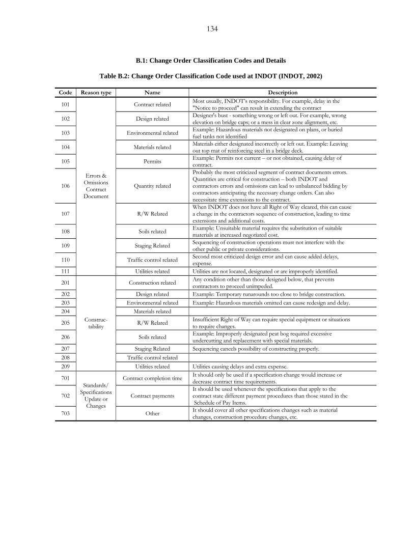
134
B.1: Change Order Classification Codes and Details
Table B.2: Change Order Classification Code used at INDOT (INDOT, 2002)
Code Reason type Name Description
101 Contract related Most usually, INDOT’s responsibility. For example, delay in the "Notice to proceed" can result in extending the contract
102 Design related Designer's bust - something wrong or left out. For example, wrong elevation on bridge caps; or a mess in clear zone alignment, etc.
103 Environmental related Example: Hazardous materials not designated on plans, or buried fuel tanks not identified
104 Materials related Materials either designated incorrectly or left out. Example: Leaving out top mat of reinforcing steel in a bridge deck.
105 Permits Example: Permits not current – or not obtained, causing delay of contract.
106 Quantity related
Probably the most criticized segment of contract documents errors. Quantities are critical for construction – both INDOT and contractors errors and omissions can lead to unbalanced bidding by contractors anticipating the necessary change orders. Can also necessitate time extensions to the contract.
107 R/W Related When INDOT does not have all Right of Way cleared, this can cause a change in the contractors sequence of construction, leading to time extensions and additional costs.
108 Soils related Example: Unsuitable material requires the substitution of suitable materials at increased negotiated cost.
109 Staging Related Sequencing of construction operations must not interfere with the other public or private considerations.
110 Traffic control related Second most criticized design error and can cause added delays, expense.
111
Errors & Omissions Contract
Document
Utilities related Utilities are not located, designated or are improperly identified.
201 Construction related Any condition other than those designed below, that prevents contractors to proceed unimpeded.
202 Design related Example: Temporary runarounds too close to bridge construction. 203 Environmental related Example: Hazardous materials omitted can cause redesign and delay. 204 Materials related
205 R/W Related Insufficient Right of Way can require special equipment or situations to require changes.
206 Soils related Example: Improperly designated peat bog required excessive undercutting and replacement with special materials.
207 Staging Related Sequencing cancels possibility of constructing properly. 208 Traffic control related 209
Construc- tability
Utilities related Utilities causing delays and extra expense.
701 Contract completion time It should only be used if a specification change would increase or decrease contract time requirements.
702 Contract payments It should be used whenever the specifications that apply to the contract state different payment procedures than those stated in the Schedule of Pay Items.
703
Standards/ Specifications
Update or Changes
Other It should cover all other specifications changes such as material changes, construction procedure changes, etc.
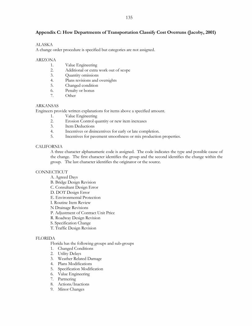
135
Appendix C: How Departments of Transportation Classify Cost Overruns (Jacoby, 2001)
ALASKA A change order procedure is specified but categories are not assigned. ARIZONA
1. Value Engineering 2. Additional or extra work out of scope 3. Quantity omissions 4. Plans revisions and oversights 5. Changed condition 6. Penalty or bonus 7. Other
ARKANSAS Engineers provide written explanations for items above a specified amount.
1. Value Engineering 2. Erosion Control quantity or new item increases 3. Item Deductions 4. Incentives or disincentives for early or late completion. 5. Incentives for pavement smoothness or mix production properties.
CALIFORNIA
A three character alphanumeric code is assigned. The code indicates the type and possible cause of the change. The first character identifies the group and the second identifies the change within the group. The last character identifies the originator or the source.
CONNECTICUT
A. Agreed Days B. Bridge Design Revision C. Consultant Design Error D. DOT Design Error E. Environmental Protection I. Routine Item Review N Drainage Revisions P. Adjustment of Contract Unit Price R. Roadway Design Revision S. Specification Change T. Traffic Design Revision
FLORIDA Florida has the following groups and sub-groups 1. Changed Conditions 2. Utility Delays 3. Weather Related Damage 4. Plans Modifications 5. Specification Modification 6. Value Engineering 7. Partnering 8. Actions/Inactions 9. Minor Changes
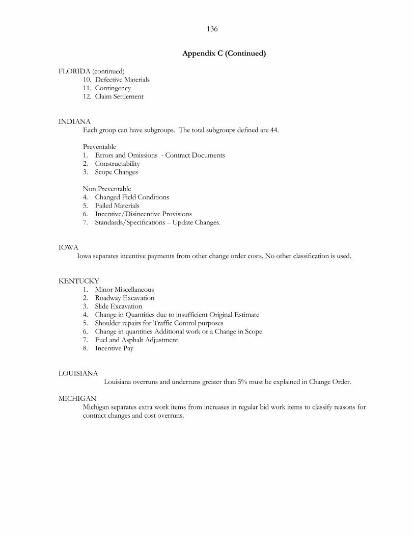
136
Appendix C (Continued)
FLORIDA (continued) 10. Defective Materials 11. Contingency 12. Claim Settlement
INDIANA
Each group can have subgroups. The total subgroups defined are 44. Preventable 1. Errors and Omissions - Contract Documents 2. Constructability 3. Scope Changes Non Preventable 4. Changed Field Conditions 5. Failed Materials 6. Incentive/Disincentive Provisions 7. Standards/Specifications – Update Changes.
IOWA Iowa separates incentive payments from other change order costs. No other classification is used. KENTUCKY
1. Minor Miscellaneous 2. Roadway Excavation 3. Slide Excavation 4. Change in Quantities due to insufficient Original Estimate 5. Shoulder repairs for Traffic Control purposes 6. Change in quantities Additional work or a Change in Scope 7. Fuel and Asphalt Adjustment. 8. Incentive Pay
LOUISIANA Louisiana overruns and underruns greater than 5% must be explained in Change Order. MICHIGAN
Michigan separates extra work items from increases in regular bid work items to classify reasons for contract changes and cost overruns.
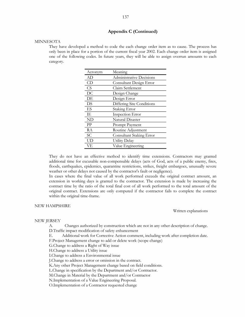
137
Appendix C (Continued) MINNESOTA
They have developed a method to code the each change order item as to cause. The process has only been in place for a portion of the current fiscal year 2002. Each change order item is assigned one of the following codes. In future years, they will be able to assign overrun amounts to each category.
Acronym Meaning AD Administrative Decisions CD Consultant Design Error CS Claim Settlement DC Design Change DE Design Error DS Differing Site Conditions ES Staking Error IE Inspection Error ND Natural Disaster PP Prompt Payment RA Routine Adjustment SC Consultant Staking Error UD Utility Delay VE Value Engineering
They do not have an effective method to identify time extensions. Contractors may granted additional time for excusable non-compensable delays (acts of God, acts of a public enemy, fires, floods, earthquakes, epidemics, quarantine restrictions, strikes, freight embargoes, unusually severe weather or other delays not caused by the contractor's fault or negligence). In cases where the final value of all work performed exceeds the original contract amount, an extension in working days is granted to the contractor. The extension is made by increasing the contract time by the ratio of the total final cost of all work performed to the total amount of the original contract. Extensions are only computed if the contractor fails to complete the contract within the original time-frame.
NEW HAMPSHIRE Written explanations NEW JERSEY
A. Changes authorized by construction which are not in any other description of change. D.Traffic impact modification of safety enhancement E. Additional work for Corrective Action comment, including work after completion date. F.Project Management change to add or delete work (scope change) G.Change to address a Right of Way issue H.Change to address a Utility issue I.Change to address a Environmental issue J.Change to address a error or omission in the contract. K.Any other Project Management change based on field conditions. L.Change in specification by the Department and/or Contractor. M.Change in Material by the Department and/or Contractor N.Implementation of a Value Engineering Proposal. O.Implementation of a Contractor requested change
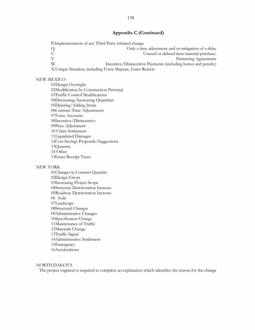
138
Appendix C (Continued) P.Implementation of any Third Party initiated change Q. Only a time adjustment and or mitigation of a delay U. Unused or deleted item material purchase. V. Partnering Agreements W. Incentive/Disincentive Payments (including bonus and penalty) X.Unique Situation, including Force Majeure, Enter Reason
NEW MEXICO
01Design Oversight 02Modification by Construction Personal 03Traffic Control Modifications 04Decreasing/Increasing Quantities 05Deleting/Adding Items 06Contract Time Adjustments 07Force Accounts 08Incentive/Disincentive 09Price Adjustment 10 Claim Settlement 11Liquidated Damages 12Cost Savings Proposals/Suggestions 13Quantity 14 Other 15Grass Receipt Taxes
NEW YORK
01Changes in Contract Quantity 02Design Errors 03Increasing Project Scope 04Structure Deterioration Increase 05Roadway Deterioration Increase 06 Soils 07Landscape 08Structural Changes 09Administrative Changes 10Specification Change 11Maintenance of Traffic 12Materials Change. 13Traffic Signal 14Administrative Settlement 15Emergency 16Accelerations.
NORTH DAKOTA The project engineer is required to complete an explanation which identifies the reason for the change
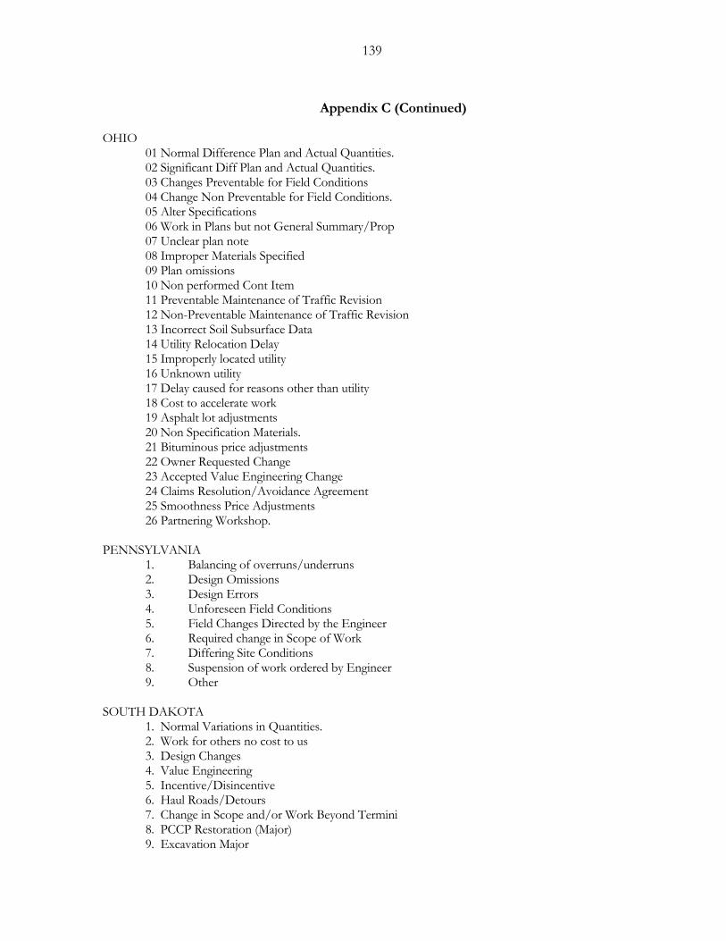
139
Appendix C (Continued)
OHIO 01 Normal Difference Plan and Actual Quantities. 02 Significant Diff Plan and Actual Quantities. 03 Changes Preventable for Field Conditions 04 Change Non Preventable for Field Conditions. 05 Alter Specifications 06 Work in Plans but not General Summary/Prop 07 Unclear plan note 08 Improper Materials Specified 09 Plan omissions 10 Non performed Cont Item 11 Preventable Maintenance of Traffic Revision 12 Non-Preventable Maintenance of Traffic Revision 13 Incorrect Soil Subsurface Data 14 Utility Relocation Delay 15 Improperly located utility 16 Unknown utility 17 Delay caused for reasons other than utility 18 Cost to accelerate work 19 Asphalt lot adjustments 20 Non Specification Materials. 21 Bituminous price adjustments 22 Owner Requested Change 23 Accepted Value Engineering Change 24 Claims Resolution/Avoidance Agreement 25 Smoothness Price Adjustments 26 Partnering Workshop. PENNSYLVANIA
1. Balancing of overruns/underruns 2. Design Omissions 3. Design Errors 4. Unforeseen Field Conditions 5. Field Changes Directed by the Engineer 6. Required change in Scope of Work 7. Differing Site Conditions 8. Suspension of work ordered by Engineer 9. Other
SOUTH DAKOTA
1. Normal Variations in Quantities. 2. Work for others no cost to us 3. Design Changes 4. Value Engineering 5. Incentive/Disincentive 6. Haul Roads/Detours 7. Change in Scope and/or Work Beyond Termini 8. PCCP Restoration (Major) 9. Excavation Major
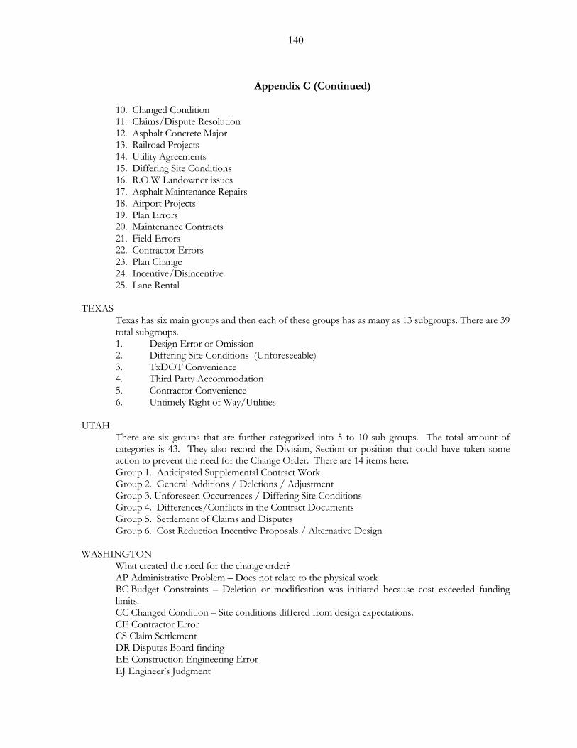
140
Appendix C (Continued)
10. Changed Condition 11. Claims/Dispute Resolution 12. Asphalt Concrete Major 13. Railroad Projects 14. Utility Agreements 15. Differing Site Conditions 16. R.O.W Landowner issues 17. Asphalt Maintenance Repairs 18. Airport Projects 19. Plan Errors 20. Maintenance Contracts 21. Field Errors 22. Contractor Errors 23. Plan Change 24. Incentive/Disincentive 25. Lane Rental
TEXAS
Texas has six main groups and then each of these groups has as many as 13 subgroups. There are 39 total subgroups. 1. Design Error or Omission 2. Differing Site Conditions (Unforeseeable) 3. TxDOT Convenience 4. Third Party Accommodation 5. Contractor Convenience 6. Untimely Right of Way/Utilities
UTAH
There are six groups that are further categorized into 5 to 10 sub groups. The total amount of categories is 43. They also record the Division, Section or position that could have taken some action to prevent the need for the Change Order. There are 14 items here. Group 1. Anticipated Supplemental Contract Work Group 2. General Additions / Deletions / Adjustment Group 3. Unforeseen Occurrences / Differing Site Conditions Group 4. Differences/Conflicts in the Contract Documents Group 5. Settlement of Claims and Disputes Group 6. Cost Reduction Incentive Proposals / Alternative Design
WASHINGTON
What created the need for the change order? AP Administrative Problem – Does not relate to the physical work BC Budget Constraints – Deletion or modification was initiated because cost exceeded funding limits. CC Changed Condition – Site conditions differed from design expectations. CE Contractor Error CS Claim Settlement DR Disputes Board finding EE Construction Engineering Error EJ Engineer’s Judgment
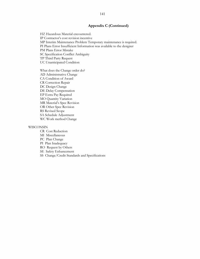
141
Appendix C (Continued) HZ Hazardous Material encountered. IP Contractor’s cost revision incentive MP Interim Maintenance Problem Temporary maintenance is required. PI Plans Error Insufficient Information was available to the designer PM Plans Error Mistake SC Specification Conflict Ambiguity TP Third Party Request UC Unanticipated Condition
What does the Change order do? AD Administrative Change CA Condition of Award CR Correction Repair DC Design Change DE Delay Compensation EP Extra Pay Required MO Quantity Variation MR Material’s Spec Revision OR Other Spec Revision RS Revised Scope SA Schedule Adjustment WC Work method Change
WISCONSIN
CR Cost Reduction MI Miscellaneous PC Plan Change PI Plan Inadequacy RO Request by Others SE Safety Enhancement SS Change/Credit Standards and Specifications
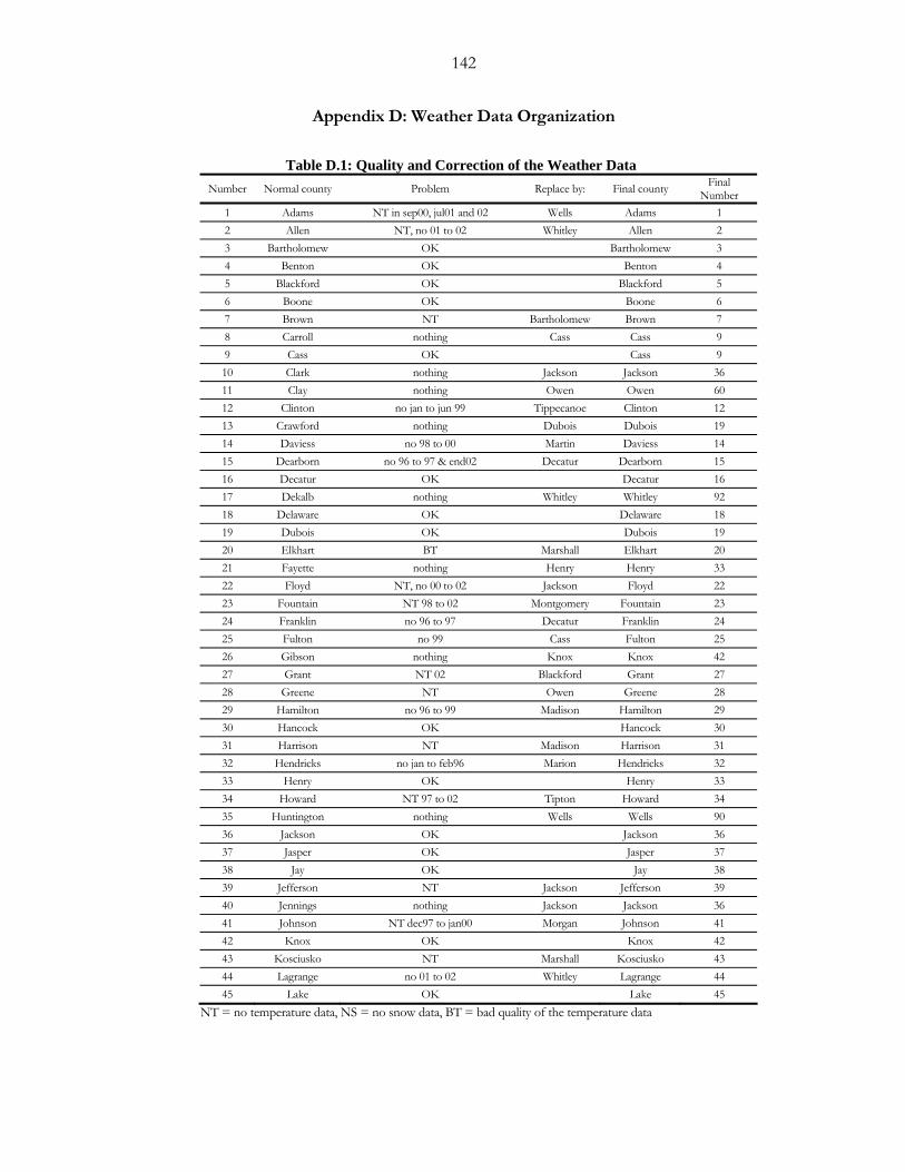
142
Appendix D: Weather Data Organization
Table D.1: Quality and Correction of the Weather Data
Number Normal county Problem Replace by: Final county Final Number
1 Adams NT in sep00, jul01 and 02 Wells Adams 1 2 Allen NT, no 01 to 02 Whitley Allen 2 3 Bartholomew OK Bartholomew 3 4 Benton OK Benton 4 5 Blackford OK Blackford 5 6 Boone OK Boone 6 7 Brown NT Bartholomew Brown 7 8 Carroll nothing Cass Cass 9 9 Cass OK Cass 9 10 Clark nothing Jackson Jackson 36 11 Clay nothing Owen Owen 60 12 Clinton no jan to jun 99 Tippecanoe Clinton 12 13 Crawford nothing Dubois Dubois 19 14 Daviess no 98 to 00 Martin Daviess 14 15 Dearborn no 96 to 97 & end02 Decatur Dearborn 15 16 Decatur OK Decatur 16 17 Dekalb nothing Whitley Whitley 92 18 Delaware OK Delaware 18 19 Dubois OK Dubois 19 20 Elkhart BT Marshall Elkhart 20 21 Fayette nothing Henry Henry 33 22 Floyd NT, no 00 to 02 Jackson Floyd 22 23 Fountain NT 98 to 02 Montgomery Fountain 23 24 Franklin no 96 to 97 Decatur Franklin 24 25 Fulton no 99 Cass Fulton 25 26 Gibson nothing Knox Knox 42 27 Grant NT 02 Blackford Grant 27 28 Greene NT Owen Greene 28 29 Hamilton no 96 to 99 Madison Hamilton 29 30 Hancock OK Hancock 30 31 Harrison NT Madison Harrison 31 32 Hendricks no jan to feb96 Marion Hendricks 32 33 Henry OK Henry 33 34 Howard NT 97 to 02 Tipton Howard 34 35 Huntington nothing Wells Wells 90 36 Jackson OK Jackson 36 37 Jasper OK Jasper 37 38 Jay OK Jay 38 39 Jefferson NT Jackson Jefferson 39 40 Jennings nothing Jackson Jackson 36 41 Johnson NT dec97 to jan00 Morgan Johnson 41 42 Knox OK Knox 42 43 Kosciusko NT Marshall Kosciusko 43 44 Lagrange no 01 to 02 Whitley Lagrange 44 45 Lake OK Lake 45
NT = no temperature data, NS = no snow data, BT = bad quality of the temperature data
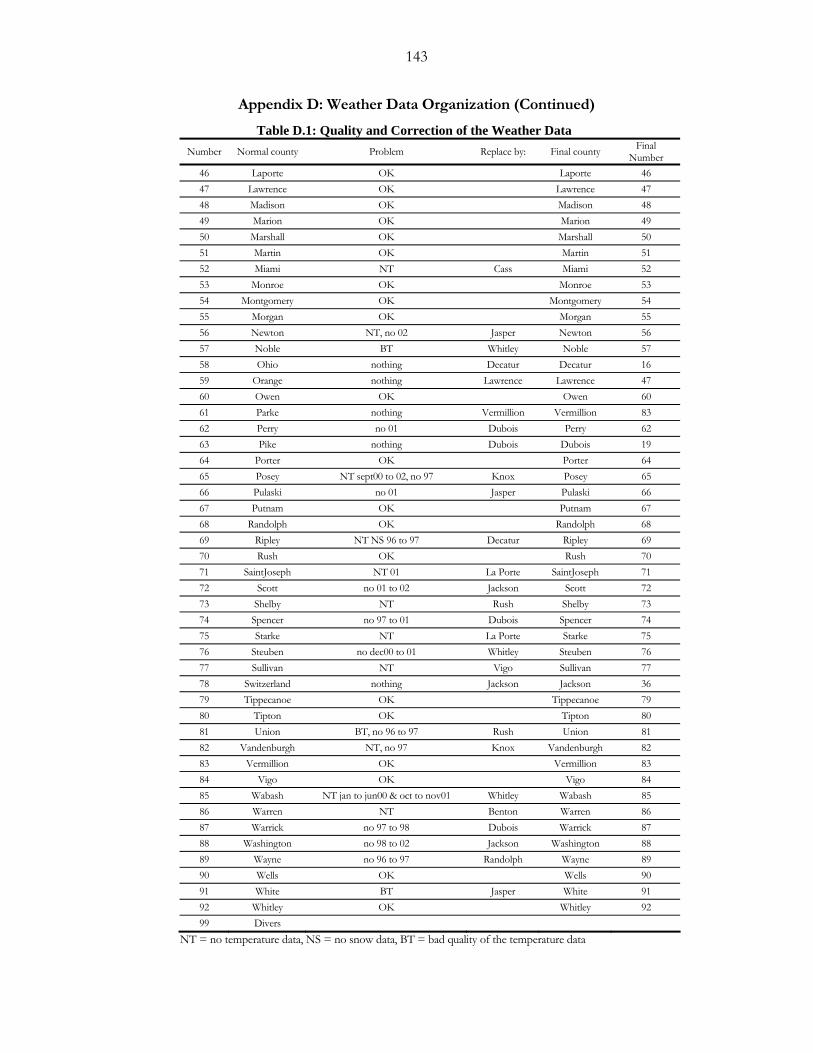
143
Appendix D: Weather Data Organization (Continued)
Table D.1: Quality and Correction of the Weather Data Number Normal county Problem Replace by: Final county Final
Number 46 Laporte OK Laporte 46 47 Lawrence OK Lawrence 47 48 Madison OK Madison 48 49 Marion OK Marion 49 50 Marshall OK Marshall 50 51 Martin OK Martin 51 52 Miami NT Cass Miami 52 53 Monroe OK Monroe 53 54 Montgomery OK Montgomery 54 55 Morgan OK Morgan 55 56 Newton NT, no 02 Jasper Newton 56 57 Noble BT Whitley Noble 57 58 Ohio nothing Decatur Decatur 16 59 Orange nothing Lawrence Lawrence 47 60 Owen OK Owen 60 61 Parke nothing Vermillion Vermillion 83 62 Perry no 01 Dubois Perry 62 63 Pike nothing Dubois Dubois 19 64 Porter OK Porter 64 65 Posey NT sept00 to 02, no 97 Knox Posey 65 66 Pulaski no 01 Jasper Pulaski 66 67 Putnam OK Putnam 67 68 Randolph OK Randolph 68 69 Ripley NT NS 96 to 97 Decatur Ripley 69 70 Rush OK Rush 70 71 SaintJoseph NT 01 La Porte SaintJoseph 71 72 Scott no 01 to 02 Jackson Scott 72 73 Shelby NT Rush Shelby 73 74 Spencer no 97 to 01 Dubois Spencer 74 75 Starke NT La Porte Starke 75 76 Steuben no dec00 to 01 Whitley Steuben 76 77 Sullivan NT Vigo Sullivan 77 78 Switzerland nothing Jackson Jackson 36 79 Tippecanoe OK Tippecanoe 79 80 Tipton OK Tipton 80 81 Union BT, no 96 to 97 Rush Union 81 82 Vandenburgh NT, no 97 Knox Vandenburgh 82 83 Vermillion OK Vermillion 83 84 Vigo OK Vigo 84 85 Wabash NT jan to jun00 & oct to nov01 Whitley Wabash 85 86 Warren NT Benton Warren 86 87 Warrick no 97 to 98 Dubois Warrick 87 88 Washington no 98 to 02 Jackson Washington 88 89 Wayne no 96 to 97 Randolph Wayne 89 90 Wells OK Wells 90 91 White BT Jasper White 91 92 Whitley OK Whitley 92 99 Divers
NT = no temperature data, NS = no snow data, BT = bad quality of the temperature data
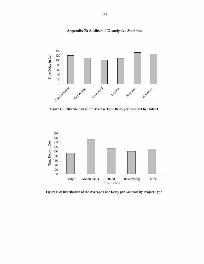
144
Appendix E: Additional Descriptive Statistics
020406080
100120140
Crawfor
dsville
Fort W
ayne
Greenfi
eld
Laporte
Seym
our
Vincen
nes
Tim
e D
elay
in D
ay
Figure E.1: Distribution of the Average Time Delay per Contract by District
020406080
100120140160180
Bridge Maintenance RoadConstruction
Resurfacing Traffic
Tim
e D
elay
in D
ay
Figure E.2: Distribution of the Average Time Delay per Contract by Project Type
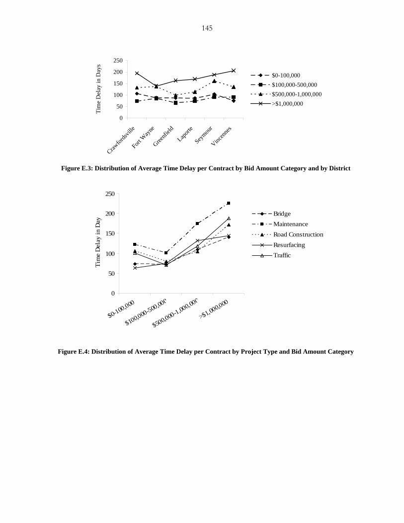
145
0
50
100
150
200
250
Crawfor
dsville
Fort W
ayne
Greenfi
eld
Laport
e
Seymou
r
Vincen
nes
Tim
e D
elay
in D
ays
$0-100,000$100,000-500,000$500,000-1,000,000>$1,000,000
Figure E.3: Distribution of Average Time Delay per Contract by Bid Amount Category and by District
0
50
100
150
200
250
$0-100,000
$100,000-500,000
$500,000-1,000,000
>$1,000,000
Tim
e D
elay
in D
ay
BridgeMaintenanceRoad ConstructionResurfacingTraffic
Figure E.4: Distribution of Average Time Delay per Contract by Project Type and Bid Amount Category
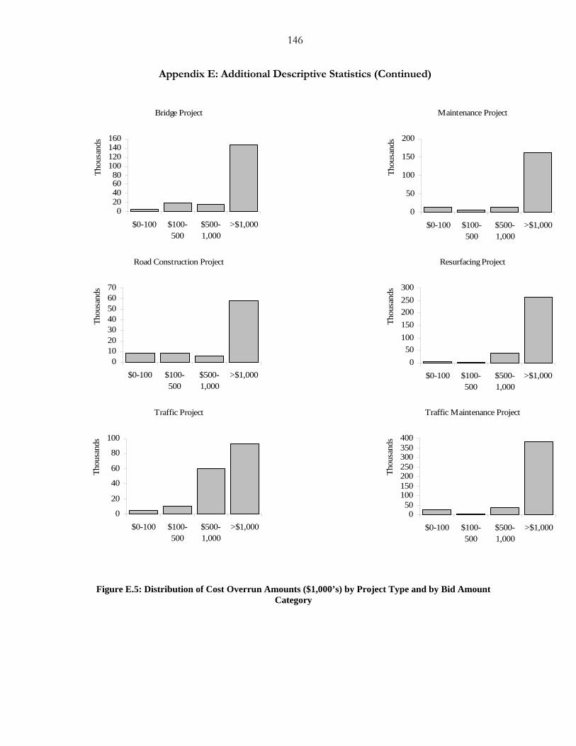
146
Appendix E: Additional Descriptive Statistics (Continued)
Bridge Project
020406080
100120140160
$0-100 $100-500
$500-1,000
>$1,000
Thou
sand
s
Maintenance Project
0
50
100
150
200
$0-100 $100-500
$500-1,000
>$1,000
Thou
sand
s
Road Construction Project
010203040506070
$0-100 $100-500
$500-1,000
>$1,000
Thou
sand
s
Resurfacing Project
050
100150200250300
$0-100 $100-500
$500-1,000
>$1,000
Thou
sand
s
Traffic Project
0
20
40
60
80
100
$0-100 $100-500
$500-1,000
>$1,000
Thou
sand
s
Traffic Maintenance Project
050
100150200250300350400
$0-100 $100-500
$500-1,000
>$1,000
Thou
sand
s
Figure E.5: Distribution of Cost Overrun Amounts ($1,000’s) by Project Type and by Bid Amount Category
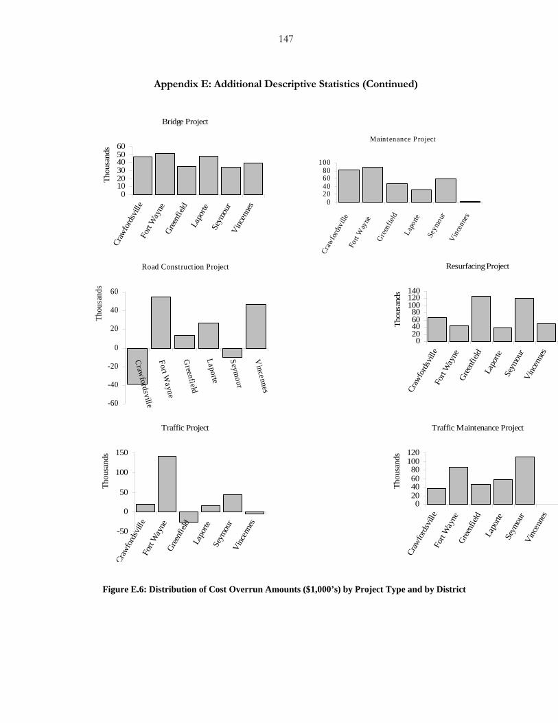
147
Appendix E: Additional Descriptive Statistics (Continued)
Bridge Project
0102030405060
Craw
ford
svill
eFo
rt W
ayne
Gree
nfiel
dLa
porte
Seym
our
Vinc
enne
s
Thou
sand
s
Road Construction Project
-60
-40
-20
0
20
40
60
Crawfordsville
Fort Wayne
Greenfield
Laporte
Seymour
Vincennes
Thou
sand
s
Resurfacing Project
020406080
100120140
Craw
ford
svill
eFo
rt W
ayne
Gree
nfiel
dLa
porte
Seym
our
Vinc
enne
s
Thou
sand
s
Traffic Project
-50
0
50
100
150
Craw
ford
svill
eFo
rt W
ayne
Gree
nfiel
dLa
porte
Seym
our
Vinc
enne
s
Thou
sand
s
Traffic Maintenance Project
020406080
100120
Craw
ford
svill
eFo
rt W
ayne
Gree
nfiel
dLa
porte
Seym
our
Vinc
enne
s
Thou
sand
s
Figure E.6: Distribution of Cost Overrun Amounts ($1,000’s) by Project Type and by District
Maintenance P roject
020406080
100
Craw
ford
svill
eFo
rt W
ayne
Green
field
Lapo
rte
Seym
our
Vince
nnes
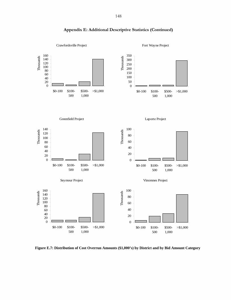
148
Appendix E: Additional Descriptive Statistics (Continued)
Crawfordsville Project
020406080
100120140160
$0-100 $100-500
$500-1,000
>$1,000
Thou
sand
s
Fort Wayne Project
050
100150200250300350
$0-100 $100-500
$500-1,000
>$1,000
Thou
sand
s
Greenfield Project
020406080
100120140
$0-100 $100-500
$500-1,000
>$1,000
Thou
sand
s
Laporte Project
0
20
40
60
80
100
$0-100 $100-500
$500-1,000
>$1,000
Thou
sand
s
Seymour Project
020406080
100120140160
$0-100 $100-500
$500-1,000
>$1,000
Thou
sand
s
Vincennes Project
0
20
40
60
80
100
$0-100 $100-500
$500-1,000
>$1,000
Thou
sand
s
Figure E.7: Distribution of Cost Overrun Amounts ($1,000’s) by District and by Bid Amount Category
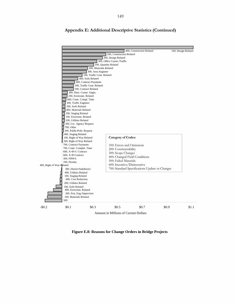
149
Appendix E: Additional Descriptive Statistics (Continued)
100, Permits300, FHWA600, A+B Contract600, A+B+C Contract700, Contr. Complet. Time700, Contract Payments200, Right of Way Related100, Right of Way Related400, Staging Related300, Public/Polit. Request700, Other300, Loc. Agency Request100, Utilities Related100, Environm. Related200, Staging Related400, Materials Related200, Soils Related300, Traffic Engineer600, Contr. Compl. Time200, Environm. Related300, Distr. Constr. Engin.
100, Contract Related200, Traffic Cont. Related600, Contract Payments
400, Soils Related100, Traffic Cont. Related
300, Area Engineer200, Materials Related
100, Quantity Related300, Office Constr./Traffic
200, Design Related200, Construction Related
400, Construction Related
400, Right of Way Related
100, Design Related
300, District/Subdistrict400, Utilities Related100, Staging Related600, Cost Reduction
200, Utilities Related100, Soils Related400, Environm. Related300, Proj. Eng./Supervisor
100, Materials Related500
-$0.2 $0.1 $0.3 $0.5 $0.7 $0.9 $1.1
Amount in Millions of Current Dollars
Figure E.8: Reasons for Change Orders in Bridge Projects
Category of Codes: 100: Errors and Omissions 200: Constructability 300: Scope Changes 400: Changed Field Conditions 500: Failed Materials 600: Incentive/Disincentive 700: Standard Specifications Update or Changes
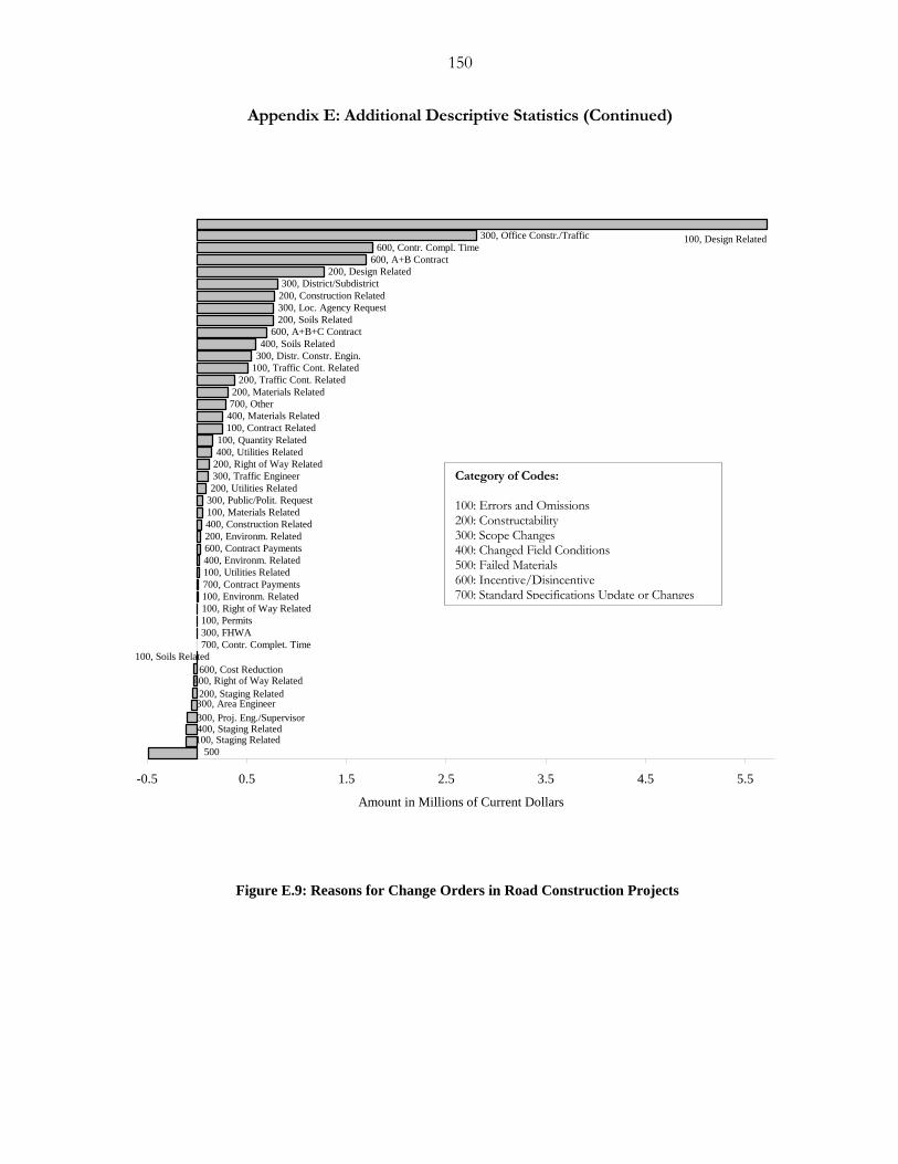
150
Appendix E: Additional Descriptive Statistics (Continued)
100, Soils Related700, Contr. Complet. Time300, FHWA100, Permits100, Right of Way Related100, Environm. Related700, Contract Payments100, Utilities Related400, Environm. Related600, Contract Payments200, Environm. Related400, Construction Related100, Materials Related300, Public/Polit. Request200, Utilities Related300, Traffic Engineer200, Right of Way Related400, Utilities Related100, Quantity Related
100, Contract Related400, Materials Related700, Other200, Materials Related
200, Traffic Cont. Related100, Traffic Cont. Related300, Distr. Constr. Engin.400, Soils Related
600, A+B+C Contract200, Soils Related300, Loc. Agency Request200, Construction Related300, District/Subdistrict
200, Design Related600, A+B Contract
600, Contr. Compl. Time300, Office Constr./Traffic
500100, Staging Related400, Staging Related300, Proj. Eng./Supervisor300, Area Engineer200, Staging Related
400, Right of Way Related600, Cost Reduction
100, Design Related
-0.5 0.5 1.5 2.5 3.5 4.5 5.5
Amount in Millions of Current Dollars
Figure E.9: Reasons for Change Orders in Road Construction Projects
Category of Codes: 100: Errors and Omissions 200: Constructability 300: Scope Changes 400: Changed Field Conditions 500: Failed Materials 600: Incentive/Disincentive 700: Standard Specifications Update or Changes
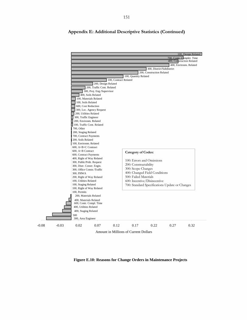
151
Appendix E: Additional Descriptive Statistics (Continued)
100, Permits100, Right of Way Related100, Staging Related100, Utilities Related200, Right of Way Related300, FHWA300, Office Constr./Traffic300, Distr. Constr. Engin.300, Public/Polit. Request400, Right of Way Related600, Contract Payments600, A+B Contract600, A+B+C Contract100, Environm. Related200, Soils Related700, Contract Payments200, Staging Related700, Other100, Traffic Cont. Related200, Environm. Related300, Traffic Engineer200, Utilities Related300, Loc. Agency Request600, Cost Reduction100, Soils Related100, Materials Related
400, Soils Related300, Proj. Eng./Supervisor
200, Traffic Cont. Related200, Design Related
100, Contract Related100, Quantity Related
200, Construction Related300, District/Subdistrict
400, Environm. Related
200, Materials Related400, Materials Related600, Contr. Compl. Time400, Utilities Related400, Staging Related
500300, Area Engineer
100, Design Related700, Contr. Complet. Time400, Construction Related
-0.08 -0.03 0.02 0.07 0.12 0.17 0.22 0.27 0.32
Amount in Millions of Current Dollars
Figure E.10: Reasons for Change Orders in Maintenance Projects
Category of Codes: 100: Errors and Omissions 200: Constructability 300: Scope Changes 400: Changed Field Conditions 500: Failed Materials 600: Incentive/Disincentive 700: Standard Specifications Update or Changes
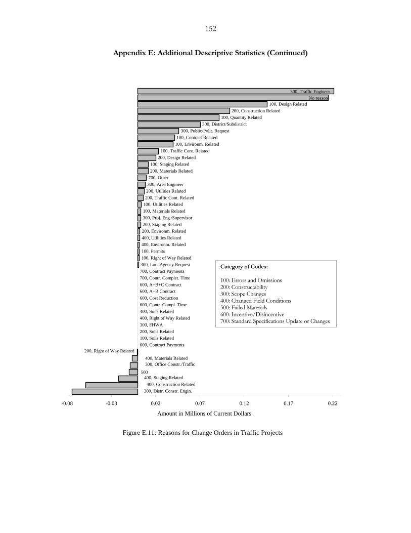
152
Appendix E: Additional Descriptive Statistics (Continued)
600, Contract Payments100, Soils Related200, Soils Related300, FHWA400, Right of Way Related400, Soils Related600, Contr. Compl. Time600, Cost Reduction600, A+B Contract600, A+B+C Contract700, Contr. Complet. Time700, Contract Payments300, Loc. Agency Request100, Right of Way Related100, Permits400, Environm. Related400, Utilities Related200, Environm. Related200, Staging Related300, Proj. Eng./Supervisor100, Materials Related100, Utilities Related200, Traffic Cont. Related200, Utilities Related300, Area Engineer700, Other200, Materials Related100, Staging Related
200, Design Related100, Traffic Cont. Related
100, Environm. Related100, Contract Related
300, Public/Polit. Request300, District/Subdistrict
100, Quantity Related200, Construction Related
100, Design Related
200, Right of Way Related
300, Traffic EngineerNo reason
400, Materials Related300, Office Constr./Traffic
500400, Staging Related
400, Construction Related300, Distr. Constr. Engin.
-0.08 -0.03 0.02 0.07 0.12 0.17 0.22
Amount in Millions of Current Dollars
Figure E.11: Reasons for Change Orders in Traffic Projects
Category of Codes: 100: Errors and Omissions 200: Constructability 300: Scope Changes 400: Changed Field Conditions 500: Failed Materials 600: Incentive/Disincentive 700: Standard Specifications Update or Changes
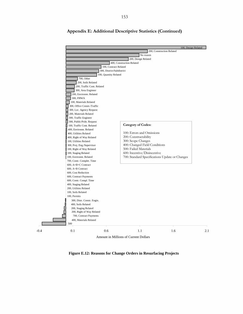
153
Appendix E: Additional Descriptive Statistics (Continued)
100, Permits100, Soils Related200, Utilities Related400, Staging Related600, Contr. Compl. Time600, Contract Payments600, Cost Reduction600, A+B Contract600, A+B+C Contract700, Contr. Complet. Time100, Environm. Related100, Staging Related100, Right of Way Related300, Proj. Eng./Supervisor100, Utilities Related400, Right of Way Related400, Utilities Related400, Environm. Related100, Traffic Cont. Related300, Public/Polit. Request300, Traffic Engineer200, Materials Related300, Loc. Agency Request300, Office Constr./Traffic100, Materials Related300, FHWA200, Environm. Related
300, Area Engineer200, Traffic Cont. Related
200, Soils Related700, Other
100, Quantity Related300, District/Subdistrict
100, Contract Related400, Construction Related
200, Design RelatedNo reason
200, Construction Related
500400, Materials Related700, Contract Payments
200, Right of Way Related200, Staging Related400, Soils Related300, Distr. Constr. Engin.
100, Design Related
-0.4 0.1 0.6 1.1 1.6 2.1
Amount in Millions of Current Dollars
Figure E.12: Reasons for Change Orders in Resurfacing Projects
Category of Codes: 100: Errors and Omissions 200: Constructability 300: Scope Changes 400: Changed Field Conditions 500: Failed Materials 600: Incentive/Disincentive 700: Standard Specifications Update or Changes
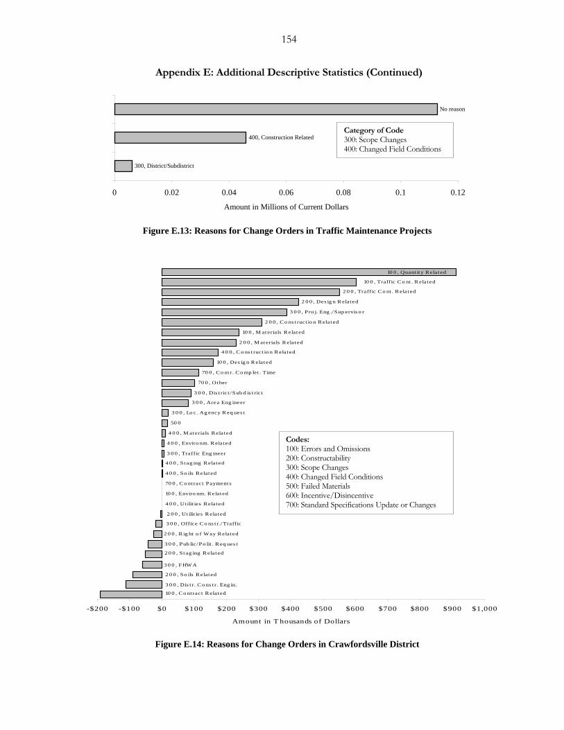
154
Appendix E: Additional Descriptive Statistics (Continued)
300, District/Subdistrict
400, Construction Related
No reason
0 0.02 0.04 0.06 0.08 0.1 0.12
Amount in Millions of Current Dollars
Figure E.13: Reasons for Change Orders in Traffic Maintenance Projects
4 0 0 , Ut ilit ies R elat ed
10 0 , Enviro nm. R elat ed
70 0 , C o nt ract Payment s
4 0 0 , So ils R elat ed
4 0 0 , S t ag ing R elat ed
3 0 0 , Traffic Eng ineer
4 0 0 , Enviro nm. R elat ed
4 0 0 , M aterials R elat ed
50 0
3 0 0 , Lo c. Ag ency R eq ues t
3 0 0 , Area Eng ineer
3 0 0 , Dis t rict /Sub d is t rict
70 0 , Other
70 0 , C o nt r. C o mp let . Time
10 0 , Des ig n R elat ed
4 0 0 , C o ns t ruct io n R elat ed
2 0 0 , M at erials R elat ed
10 0 , M at erials R elat ed
2 0 0 , C o ns t ruct io n R elat ed
3 0 0 , Pro j. Eng ./Sup ervis o r
2 0 0 , Des ig n R elat ed
2 0 0 , Traffic C o nt . R elat ed
10 0 , Traffic C o nt . R elat ed
10 0 , Quant it y R elat ed
2 0 0 , Ut ilit ies R elat ed
10 0 , C o nt ract R elat ed
3 0 0 , Dis t r. C o ns t r. Eng in.
2 0 0 , So ils R elat ed
3 0 0 , FHW A
2 0 0 , S t ag ing R elat ed
3 0 0 , Pub lic/Po lit . R eq ues t
2 0 0 , R ig ht o f Way R elat ed
3 0 0 , Office C o ns t r./Traffic
-$200 -$100 $0 $100 $200 $300 $400 $500 $600 $700 $800 $900 $1,000
Amount in T housands of Dollars
Figure E.14: Reasons for Change Orders in Crawfordsville District
Category of Code 300: Scope Changes 400: Changed Field Conditions
Codes: 100: Errors and Omissions 200: Constructability 300: Scope Changes 400: Changed Field Conditions 500: Failed Materials 600: Incentive/Disincentive 700: Standard Specifications Update or Changes
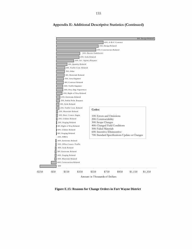
155
Appendix E: Additional Descriptive Statistics (Continued)
10 0 , S tag ing R elat ed
4 0 0 , Ut ilit ies R elat ed
10 0 , R ig ht o f Way R elat ed
2 0 0 , S tag ing R elat ed
2 0 0 , Ut ilit ies R elat ed
3 0 0 , Dis t r. C o ns t r. Eng in.
2 0 0 , M at erials R elat ed
2 0 0 , Traffic C o nt . R elat ed
10 0 , So ils R elat ed
3 0 0 , Pub lic/ Po lit . R eq ues t
2 0 0 , Enviro nm. R elated
2 0 0 , R ig ht o f Way R elated
3 0 0 , P ro j. Eng ./Sup ervis o r
3 0 0 , Traffic Eng ineer
10 0 , C o nt ract R elat ed
3 0 0 , Area Eng ineer
10 0 , M at erials R elat ed
70 0 , Ot her
10 0 , Traffic C o nt . R elated
10 0 , Quant ity R elat ed
3 0 0 , Lo c. Ag ency R eq ues t
2 0 0 , So ils R elated
2 0 0 , Des ig n R elat ed
6 0 0 , A+B +C C o nt ract
10 0 , Des ig n R elat ed
4 0 0 , Enviro nm. R elat ed
3 0 0 , Office C o ns t r./ Traffic
4 0 0 , So ils R elat ed
10 0 , Enviro nm. R elated
4 0 0 , St ag ing R elated
4 0 0 , M aterials R elated
4 0 0 , C o ns t ruct io n R elated
50 0
3 0 0 , FHWA
2 0 0 , C o ns t ruct io n R elat ed
3 0 0 , Dis t rict /Sub d is t rict
-$250 -$50 $150 $350 $550 $750 $950 $1,150 $1,350
Amount in T housands of Dollars
Figure E.15: Reasons for Change Orders in Fort Wayne District
Codes: 100: Errors and Omissions 200: Constructability 300: Scope Changes 400: Changed Field Conditions 500: Failed Materials 600: Incentive/Disincentive 700: Standard Specifications Update or Changes
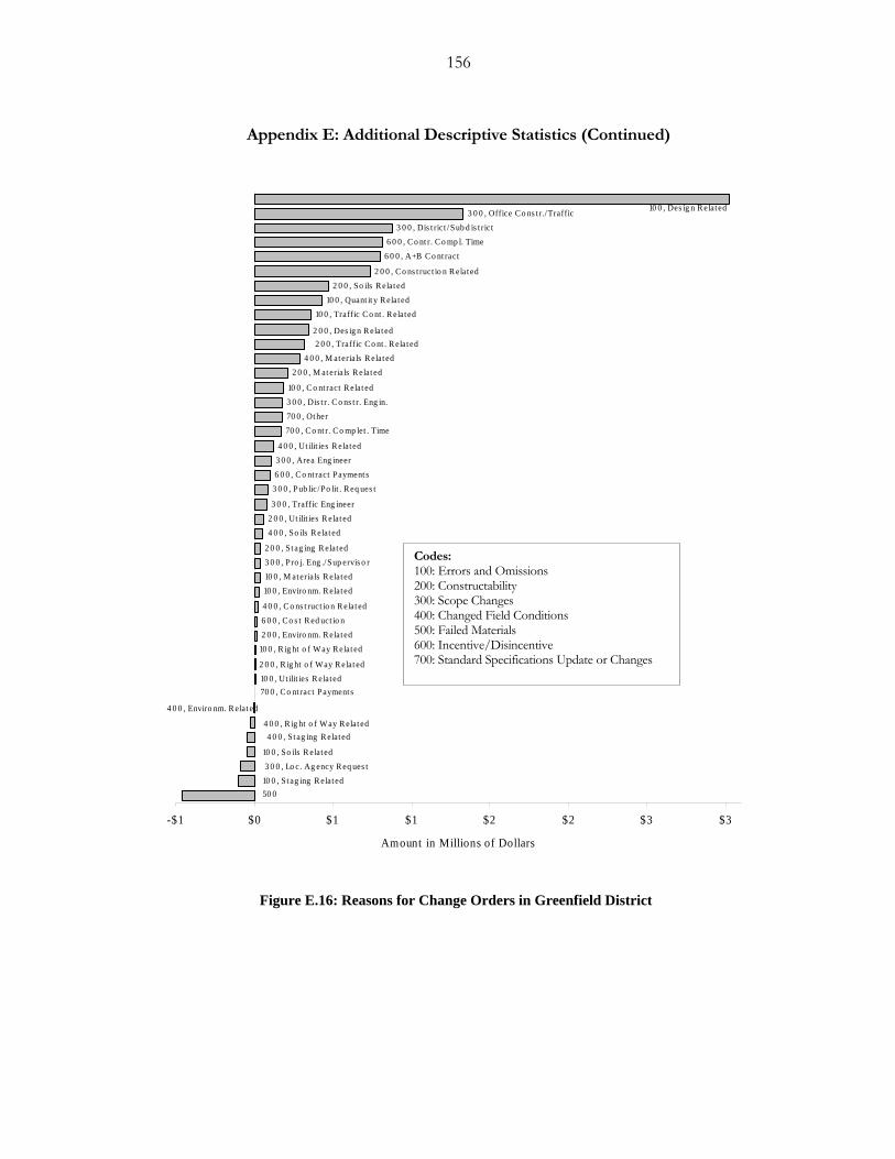
156
Appendix E: Additional Descriptive Statistics (Continued)
2 0 0 , R ig ht o f Way R elat ed
10 0 , R ig ht o f Way R elat ed2 0 0 , Enviro nm. R elated6 0 0 , Co s t R ed uct io n4 0 0 , C o ns t ruct io n R elat ed
10 0 , Enviro nm. R elated10 0 , M aterials R elated3 0 0 , Pro j. Eng ./ Sup ervis o r2 0 0 , St ag ing R elated
2 0 0 , Ut ilit ies R elat ed3 0 0 , Traffic Eng ineer
3 0 0 , Pub lic/ Po lit . R eq ues t6 0 0 , C o nt ract Payments3 0 0 , Area Eng ineer4 0 0 , Ut ilit ies R elated
70 0 , C o nt r. C o mp let . Time70 0 , Ot her3 0 0 , Dis t r. C o ns t r. Eng in.10 0 , C o nt ract R elat ed
2 0 0 , M at erials R elat ed4 0 0 , M aterials R elated
10 0 , Traffic C o nt . R elated10 0 , Quant it y R elated
2 0 0 , C o ns t ruct io n R elated
6 0 0 , A+B C o nt ract6 0 0 , C o nt r. C o mp l. Time
3 0 0 , Dis t rict /Sub d is t rict3 0 0 , Office Co ns t r./Traffic
4 0 0 , So ils R elat ed
10 0 , Des ig n R elated
2 0 0 , Traffic C o nt . R elated2 0 0 , Des ig n R elat ed
10 0 , Ut ilit ies R elated
50 010 0 , St ag ing R elated3 0 0 , Lo c. Ag ency R eq ues t
10 0 , So ils R elated
4 0 0 , St ag ing R elated4 0 0 , R ig ht o f Way R elat ed
4 0 0 , Enviro nm. R elat ed
70 0 , Co nt ract Payments
2 0 0 , So ils R elated
-$1 $0 $1 $1 $2 $2 $3 $3
Amount in Millions of Dollars
Figure E.16: Reasons for Change Orders in Greenfield District
Codes: 100: Errors and Omissions 200: Constructability 300: Scope Changes 400: Changed Field Conditions 500: Failed Materials 600: Incentive/Disincentive 700: Standard Specifications Update or Changes
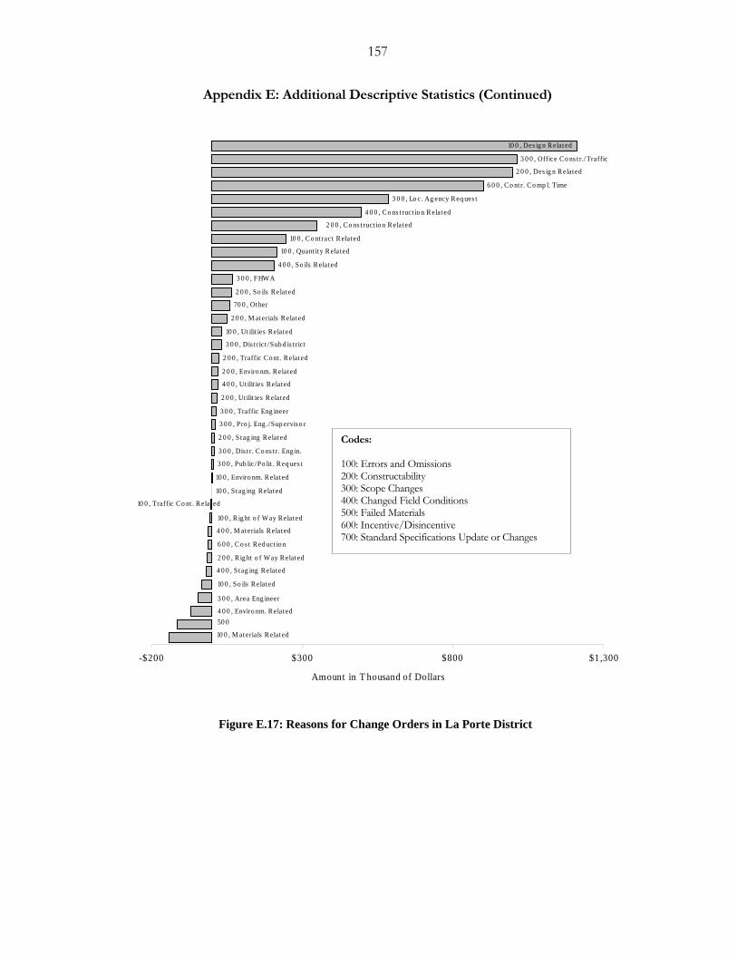
157
Appendix E: Additional Descriptive Statistics (Continued)
10 0 , Traffic C o nt . R elat ed
10 0 , St ag ing R elated
10 0 , Enviro nm. R elat ed
3 0 0 , Pub lic/Po lit . R eq ues t
3 0 0 , Dis t r. C o ns t r. Eng in.
2 0 0 , S tag ing R elat ed
3 0 0 , Pro j. Eng ./ Sup ervis o r
3 0 0 , Traffic Eng ineer
2 0 0 , Ut ilit ies R elated
4 0 0 , Ut ilit ies R elat ed
2 0 0 , Enviro nm. R elated
2 0 0 , Traffic C o nt . R elated
3 0 0 , Dis t rict /Sub d is t rict
10 0 , Ut ilit ies R elat ed
2 0 0 , M at erials R elat ed
70 0 , Ot her
2 0 0 , So ils R elated
3 0 0 , FHWA
4 0 0 , So ils R elat ed
10 0 , Quant it y R elated
10 0 , C o nt ract R elated
3 0 0 , Lo c. Ag ency R eq ues t
6 0 0 , C o nt r. C o mp l. Time
3 0 0 , Office C o ns t r./ Traffic
10 0 , Des ig n R elat ed
10 0 , R ig ht o f Way R elated
2 0 0 , Des ig n R elated
6 0 0 , C o s t R ed uct io n
2 0 0 , R ig ht o f Way R elated
4 0 0 , S tag ing R elat ed
10 0 , So ils R elated
3 0 0 , Area Eng ineer
4 0 0 , Enviro nm. R elat ed50 0
10 0 , M at erials R elat ed
4 0 0 , M at erials R elat ed
4 0 0 , C o ns t ruct io n R elat ed
2 0 0 , C o ns t ruct io n R elated
-$200 $300 $800 $1,300
Amount in T housand of Dollars
Figure E.17: Reasons for Change Orders in La Porte District
Codes: 100: Errors and Omissions 200: Constructability 300: Scope Changes 400: Changed Field Conditions 500: Failed Materials 600: Incentive/Disincentive 700: Standard Specifications Update or Changes
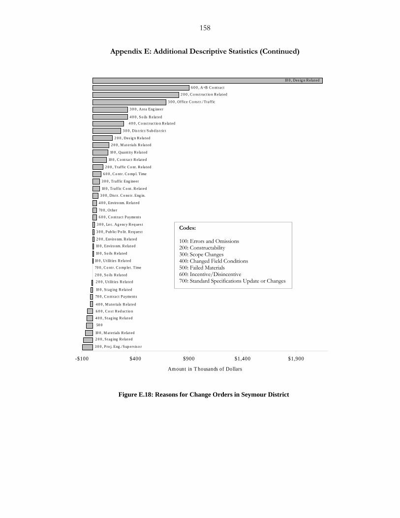
158
Appendix E: Additional Descriptive Statistics (Continued)
2 0 0 , So ils R elated
70 0 , C o nt r. C o mp let . Time
10 0 , Ut ilit ies R elated
10 0 , So ils R elated
10 0 , Enviro nm. R elat ed
2 0 0 , Enviro nm. R elated
3 0 0 , Pub lic/ Po lit . R eq ues t
3 0 0 , Lo c. Ag ency R eq ues t
6 0 0 , C o nt ract Payment s
70 0 , Ot her
4 0 0 , Enviro nm. R elat ed
3 0 0 , Dis t r. C o ns t r. Eng in.
10 0 , Traffic C o nt . R elated
3 0 0 , Traffic Eng ineer
6 0 0 , C o nt r. C o mp l. Time
2 0 0 , Traffic C o nt . R elat ed
10 0 , C o nt ract R elated
10 0 , Quant ity R elat ed
2 0 0 , M at erials R elat ed
2 0 0 , Des ig n R elat ed
3 0 0 , Dis t rict /Sub d is t rict
3 0 0 , Area Eng ineer
3 0 0 , Office C o ns t r./ Traffic
6 0 0 , A+B C o nt ract
4 0 0 , C o ns t ruct io n R elat ed4 0 0 , So ils R elat ed
10 0 , St ag ing R elated
3 0 0 , Pro j. Eng ./ Sup ervis o r
2 0 0 , S tag ing R elat ed10 0 , M at erials R elat ed
50 0
4 0 0 , S tag ing R elat ed
6 0 0 , C o s t R ed uct io n
4 0 0 , M aterials R elated
70 0 , C o nt ract Payment s
2 0 0 , C o ns t ruct io n R elat ed
2 0 0 , Ut ilit ies R elated
10 0 , Des ig n R elated
-$100 $400 $900 $1,400 $1,900
Amount in T housands of Dollars
Figure E.18: Reasons for Change Orders in Seymour District
Codes: 100: Errors and Omissions 200: Constructability 300: Scope Changes 400: Changed Field Conditions 500: Failed Materials 600: Incentive/Disincentive 700: Standard Specifications Update or Changes
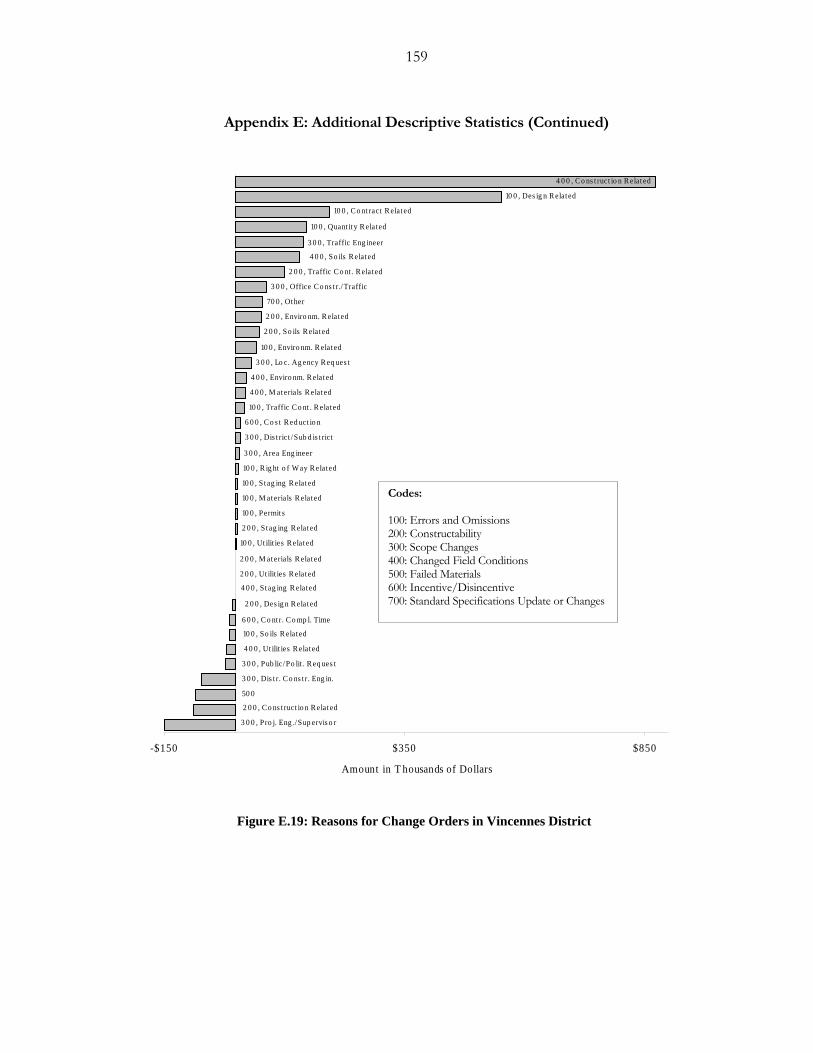
159
Appendix E: Additional Descriptive Statistics (Continued)
2 0 0 , Ut ilit ies R elat ed
2 0 0 , M at erials R elat ed
10 0 , Ut ilit ies R elat ed
2 0 0 , S tag ing R elat ed
10 0 , Permit s
10 0 , M at erials R elat ed
10 0 , S tag ing R elat ed
10 0 , R ig ht o f Way R elated
3 0 0 , Area Eng ineer
3 0 0 , Dis t rict / Sub d is t rict
6 0 0 , C o s t R ed uct io n
10 0 , Traffic C o nt . R elated
4 0 0 , M at erials R elat ed
4 0 0 , Enviro nm. R elat ed
3 0 0 , Lo c. Ag ency R eq ues t
10 0 , Enviro nm. R elat ed
2 0 0 , So ils R elat ed
2 0 0 , Enviro nm. R elated
70 0 , Ot her
3 0 0 , Office C o ns t r./ Traffic
2 0 0 , Traffic C o nt . R elated
10 0 , Quant it y R elated
10 0 , C o nt ract R elat ed
4 0 0 , C o ns t ruct io n R elat ed
4 0 0 , St ag ing R elated
10 0 , Des ig n R elated
6 0 0 , C o nt r. C o mp l. Time
10 0 , So ils R elated
4 0 0 , Ut ilit ies R elat ed
3 0 0 , Pub lic/ Po lit . R eq ues t
3 0 0 , Dis t r. C o ns t r. Eng in.
50 0
2 0 0 , C o ns t ruct io n R elat ed
3 0 0 , Pro j. Eng ./ Sup ervis o r
2 0 0 , Des ig n R elat ed
3 0 0 , Traffic Eng ineer
4 0 0 , So ils R elat ed
-$150 $350 $850
Amount in T housands of Dollars
Figure E.19: Reasons for Change Orders in Vincennes District
Codes: 100: Errors and Omissions 200: Constructability 300: Scope Changes 400: Changed Field Conditions 500: Failed Materials 600: Incentive/Disincentive 700: Standard Specifications Update or Changes
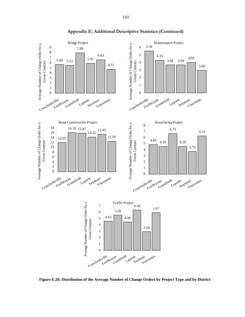
160
Appendix E: Additional Descriptive Statistics (Continued)
Bridge Project
5.66 5.51
7.96
5.916.63
4.71
0123456789
Crawfordsville
FortWayne
GreenfieldLaporte
Seymour
VincennesAve
rage
Num
ber o
f Cha
nge
Ord
er fo
r a
Giv
en C
ontra
ct
M aintenance Project5.56
4.333.68 3.69
4.05
3.00
0
1
2
3
4
5
6
Crawfordsville
FortWayne
GreenfieldLaporte
Seymour
VincennesAve
rage
Num
ber o
f Cha
nge
Ord
er fo
r a
Giv
en C
ontra
ct
Road Construction Project
12.05
16.18 15.8714.25
15.45
12.59
02468
1012141618
Crawfordsville
FortWayne
GreenfieldLaporte
Seymour
VincennesAve
rage
Num
ber o
f Cha
nge
Ord
er fo
r a
Giv
en C
ontra
ct
Resurfacing Project
4.85 4.59
6.73
4.593.73
6.31
0
1
2
3
4
5
6
7
8
Crawfordsville
FortWayne
GreenfieldLaporte
Seymour
VincennesAve
rage
Num
ber o
f Cha
nge
Ord
er fo
r a
Giv
en C
ontra
ct
Traffic Project
4.63
5.58
4.49
6.36
2.94
5.97
0
1
2
3
4
5
6
7
Crawfordsville
FortWayne
GreenfieldLaporte
Seymour
VincennesAve
rage
Num
ber o
f Cha
nge
Ord
er fo
r a
Giv
en C
ontra
ct
Figure E.20: Distribution of the Average Number of Change Orders by Project Type and by District
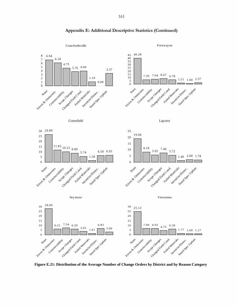
161
Appendix E: Additional Descriptive Statistics (Continued)
Crawfordsville
6.946.18
4.753.76 4.00
1.100.00
3.37
012345678
None
Errors
& Omiss
ions
Constructa
bility
Scope
Cha
nges
Changed
Field C
ond.
Failed
Mate
rials
Incen
t ive/D
isinc.
Stand S
pec U
pdate
Fortwayne
40.28
7.20 7.64 8.67 6.781.51 1.00 2.37
05
1015202530354045
None
Errors
& Omiss
ions
Constru
ctabil
ity
Scope
Cha
nges
Changed
Field C
ond.
Failed
Mate
rials
Incen
tive/D
isinc.
Stand S
pec U
pdate
Greenfield
26.89
11.85 10.23 8.895.74
1.586.50 6.93
05
1015
202530
None
Errors &
Omiss
ions
Constructa
bility
Scope
Changes
Changed
Field C
ond.
Failed
Mate
rials
Incent
ive/D
isinc.
Stand S
pec U
pdate
Laporte
19.06
8.185.92 7.46
5.72
1.46 2.00 1.78
0
5
10
15
20
25
None
Errors &
Omiss
ions
Constructa
bility
Scope
Changes
Changed
Field C
ond.
Failed
Mate
rials
Incent
ive/D
isinc.
Stand S
pec U
pdate
Seymour
28.06
6.21 7.34 6.293.65 1.61
6.833.00
05
1015
202530
None
Errors
& Omiss
ions
Constru
ctabil
ity
Scope
Cha
nges
Changed
Field C
ond.
Failed
Mate
rials
Incen
tive/D
isinc.
Stand S
pec U
pdate
Vincennes
25.12
7.00 6.924.75 6.39
1.77 1.00 1.1705
1015
202530
None
Errors
& Omiss
ions
Constru
ctabil
ity
Scope
Cha
nges
Changed
Field C
ond.
Failed
Mate
rials
Incen
tive/D
isinc.
Stand S
pec U
pdate
Figure E.21: Distribution of the Average Number of Change Orders by District and by Reason Category
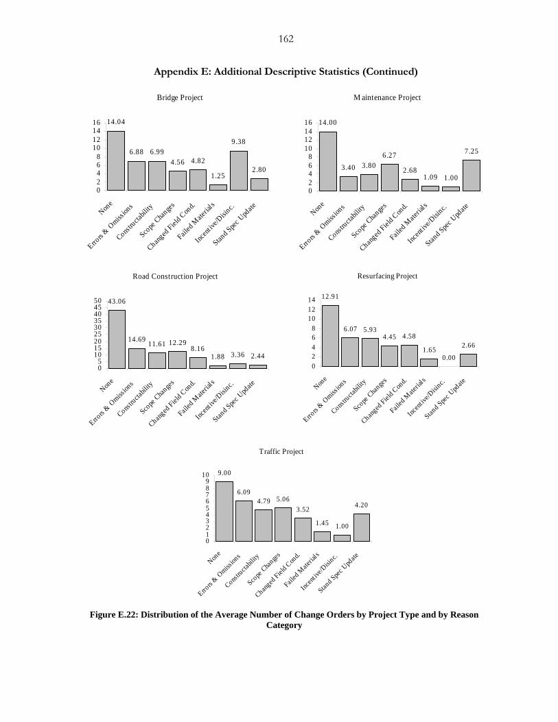
162
Appendix E: Additional Descriptive Statistics (Continued)
Bridge Project
14.04
6.88 6.994.56 4.82
1.25
9.38
2.80
02468
10121416
None
Errors &
Omiss
ions
Constructa
bility
Scope
Changes
Changed
Field C
ond.
Failed
Mate
rials
Incent
ive/D
isinc.
Stand S
pec U
pdate
M aintenance Project
14.00
3.40 3.806.27
2.681.09 1.00
7.25
02468
10121416
None
Errors &
Omiss
ions
Constructa
bility
Scope
Changes
Changed
Field C
ond.
Failed
Mate
rials
Incent
ive/D
isinc.
Stand S
pec U
pdate
Road Construction Project
43.06
14.69 11.61 12.298.16
1.88 3.36 2.4405
101520253035404550
None
Errors &
Omiss
ions
Constructa
bility
Scope
Changes
Changed
Field C
ond.
Failed
Mate
rials
Incent
ive/D
isinc.
Stand S
pec U
pdate
Resurfacing Project
12.91
6.07 5.934.45 4.58
1.650.00
2.66
02468
101214
None
Errors &
Omiss
ions
Constructa
bility
Scope
Changes
Changed
Field C
ond.
Failed
Mate
rial s
Incent
ive/D
isinc.
Stand S
pec U
pdate
Traffic Project
9.00
6.094.79 5.06
3.52
1.45 1.00
4.20
0123456789
10
None
Errors &
Omiss
ions
Constructa
bility
Scope
Changes
Changed
Field C
ond.
Failed
Mate
rials
Incent
ive/D
isinc.
Stand S
pec U
pdate
Figure E.22: Distribution of the Average Number of Change Orders by Project Type and by Reason
Category
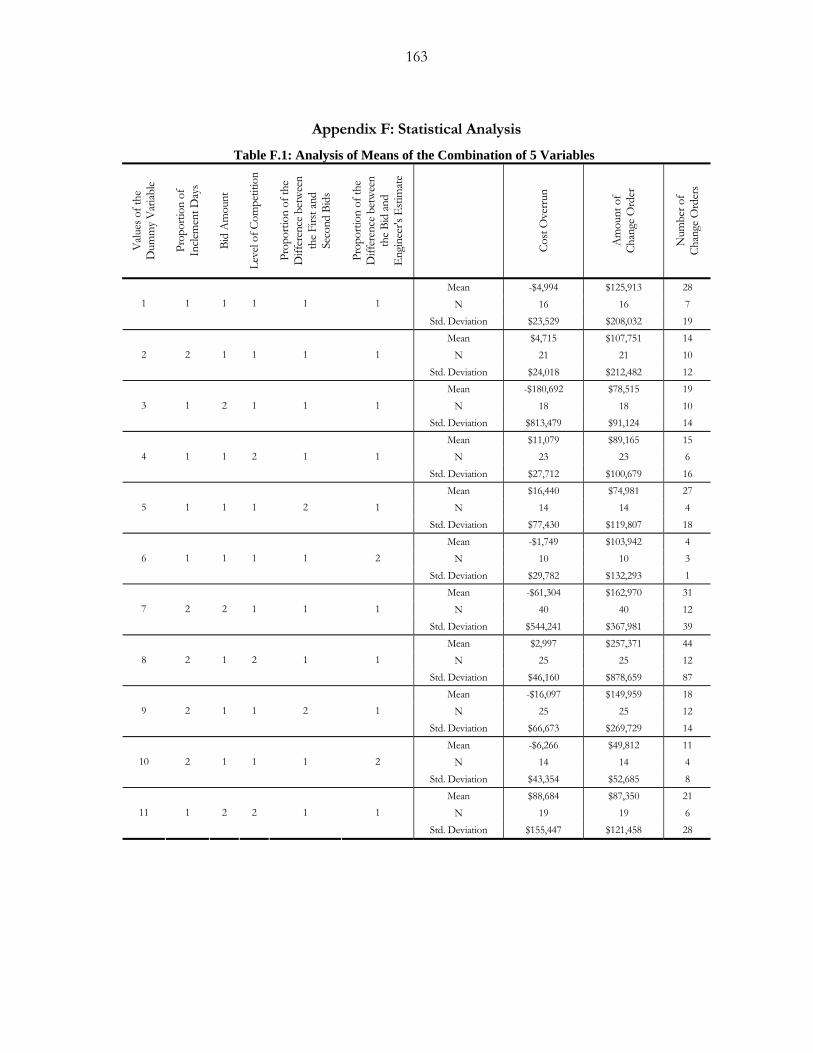
163
Appendix F: Statistical Analysis
Table F.1: Analysis of Means of the Combination of 5 Variables V
alues
of t
he
Dum
my V
ariab
le
Prop
ortio
n of
In
clem
ent D
ays
Bid
Am
ount
Leve
l of C
ompe
titio
n
Prop
ortio
n of
the
Diff
eren
ce b
etw
een
the F
irst a
nd
Seco
nd B
ids
Prop
ortio
n of
the
Diff
eren
ce b
etw
een
the B
id an
d En
gine
er's
Estim
ate
Cost
Ove
rrun
Am
ount
of
Chan
ge O
rder
Num
ber o
f Ch
ange
Ord
ers
Mean -$4,994 $125,913 28 N 16 16 7 1 1 1 1 1 1
Std. Deviation $23,529 $208,032 19 Mean $4,715 $107,751 14
N 21 21 10 2 2 1 1 1 1
Std. Deviation $24,018 $212,482 12 Mean -$180,692 $78,515 19
N 18 18 10 3 1 2 1 1 1
Std. Deviation $813,479 $91,124 14 Mean $11,079 $89,165 15
N 23 23 6 4 1 1 2 1 1
Std. Deviation $27,712 $100,679 16 Mean $16,440 $74,981 27
N 14 14 4 5 1 1 1 2 1
Std. Deviation $77,430 $119,807 18 Mean -$1,749 $103,942 4
N 10 10 3 6 1 1 1 1 2
Std. Deviation $29,782 $132,293 1 Mean -$61,304 $162,970 31
N 40 40 12 7 2 2 1 1 1
Std. Deviation $544,241 $367,981 39 Mean $2,997 $257,371 44
N 25 25 12 8 2 1 2 1 1
Std. Deviation $46,160 $878,659 87 Mean -$16,097 $149,959 18
N 25 25 12 9 2 1 1 2 1
Std. Deviation $66,673 $269,729 14 Mean -$6,266 $49,812 11
N 14 14 4 10 2 1 1 1 2
Std. Deviation $43,354 $52,685 8 Mean $88,684 $87,350 21
N 19 19 6 11 1 2 2 1 1
Std. Deviation $155,447 $121,458 28
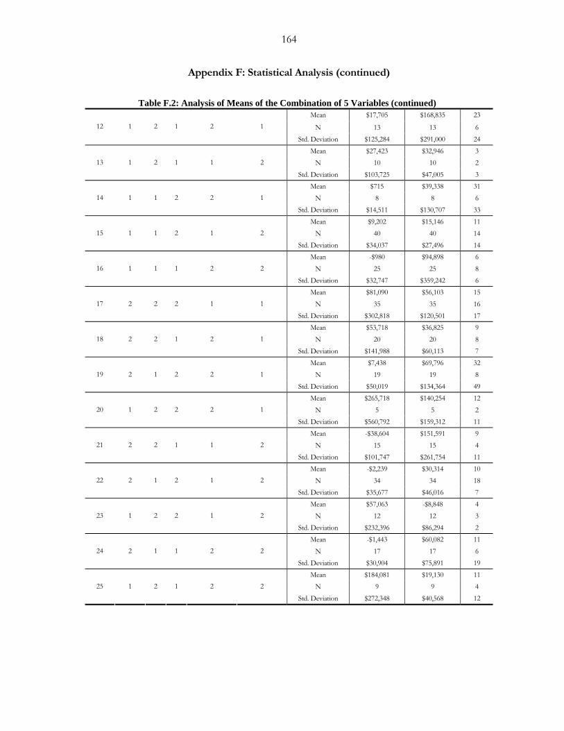
164
Appendix F: Statistical Analysis (continued)
Table F.2: Analysis of Means of the Combination of 5 Variables (continued)
Mean $17,705 $168,835 23
N 13 13 6 12 1 2 1 2 1
Std. Deviation $125,284 $291,000 24 Mean $27,423 $32,946 3
N 10 10 2 13 1 2 1 1 2
Std. Deviation $103,725 $47,005 3 Mean $715 $39,338 31
N 8 8 6 14 1 1 2 2 1
Std. Deviation $14,511 $130,707 33 Mean $9,202 $15,146 11
N 40 40 14 15 1 1 2 1 2
Std. Deviation $34,037 $27,496 14 Mean -$980 $94,898 6
N 25 25 8 16 1 1 1 2 2
Std. Deviation $32,747 $359,242 6 Mean $81,090 $56,103 15
N 35 35 16 17 2 2 2 1 1
Std. Deviation $302,818 $120,501 17 Mean $53,718 $36,825 9
N 20 20 8 18 2 2 1 2 1
Std. Deviation $141,988 $60,113 7 Mean $7,438 $69,796 32
N 19 19 8 19 2 1 2 2 1
Std. Deviation $50,019 $134,364 49 Mean $265,718 $140,254 12
N 5 5 2 20 1 2 2 2 1
Std. Deviation $560,792 $159,312 11 Mean -$38,604 $151,591 9
N 15 15 4 21 2 2 1 1 2
Std. Deviation $101,747 $261,754 11 Mean -$2,239 $30,314 10
N 34 34 18 22 2 1 2 1 2
Std. Deviation $35,677 $46,016 7 Mean $57,063 -$8,848 4
N 12 12 3 23 1 2 2 1 2
Std. Deviation $232,396 $86,294 2 Mean -$1,443 $60,082 11
N 17 17 6 24 2 1 1 2 2
Std. Deviation $30,904 $75,891 19 Mean $184,081 $19,130 11
N 9 9 4 25 1 2 1 2 2
Std. Deviation $272,348 $40,568 12
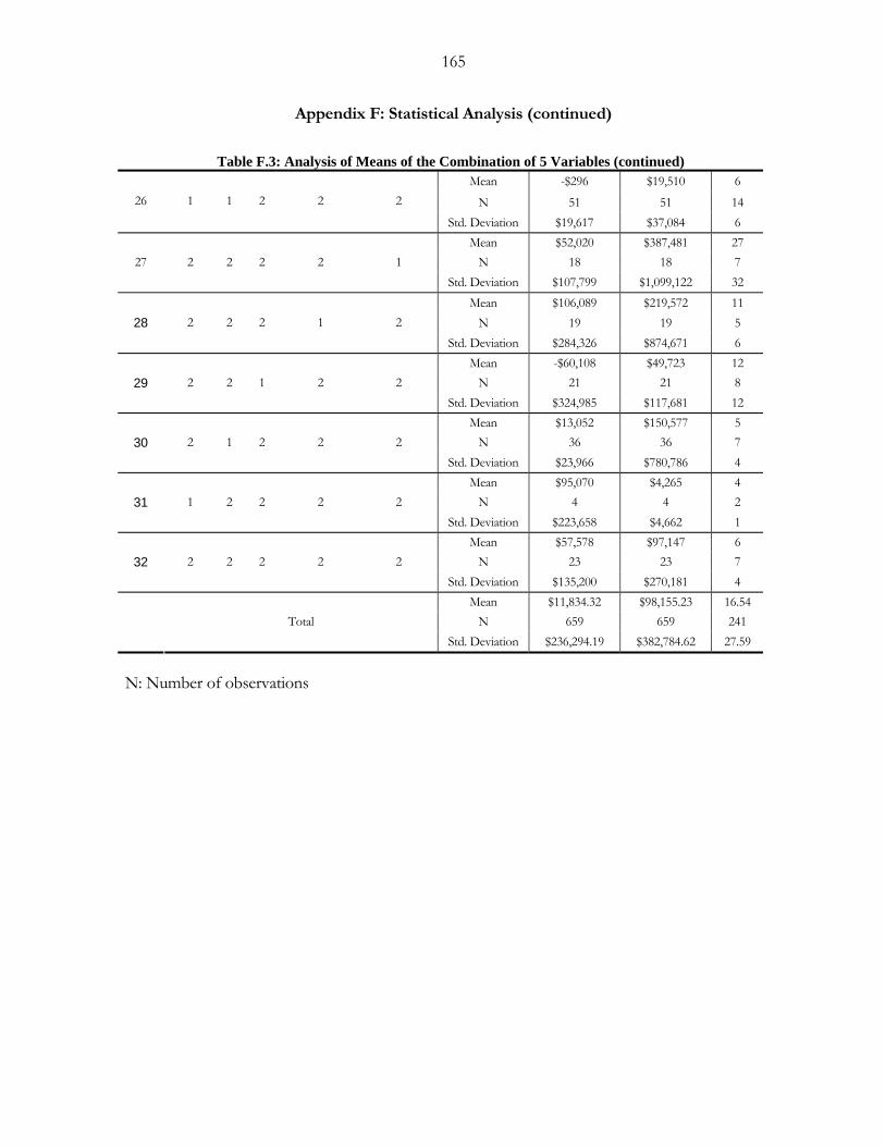
165
Appendix F: Statistical Analysis (continued)
Table F.3: Analysis of Means of the Combination of 5 Variables (continued)
Mean -$296 $19,510 6
N 51 51 14 26 1 1 2 2 2
Std. Deviation $19,617 $37,084 6 Mean $52,020 $387,481 27
N 18 18 7 27 2 2 2 2 1 Std. Deviation $107,799 $1,099,122 32
Mean $106,089 $219,572 11 N 19 19 5 28 2 2 2 1 2
Std. Deviation $284,326 $874,671 6 Mean -$60,108 $49,723 12
N 21 21 8 29 2 2 1 2 2 Std. Deviation $324,985 $117,681 12
Mean $13,052 $150,577 5 N 36 36 7 30 2 1 2 2 2
Std. Deviation $23,966 $780,786 4 Mean $95,070 $4,265 4
N 4 4 2 31 1 2 2 2 2 Std. Deviation $223,658 $4,662 1
Mean $57,578 $97,147 6 N 23 23 7 32 2 2 2 2 2
Std. Deviation $135,200 $270,181 4 Mean $11,834.32 $98,155.23 16.54
N 659 659 241 Total Std. Deviation $236,294.19 $382,784.62 27.59
N: Number of observations
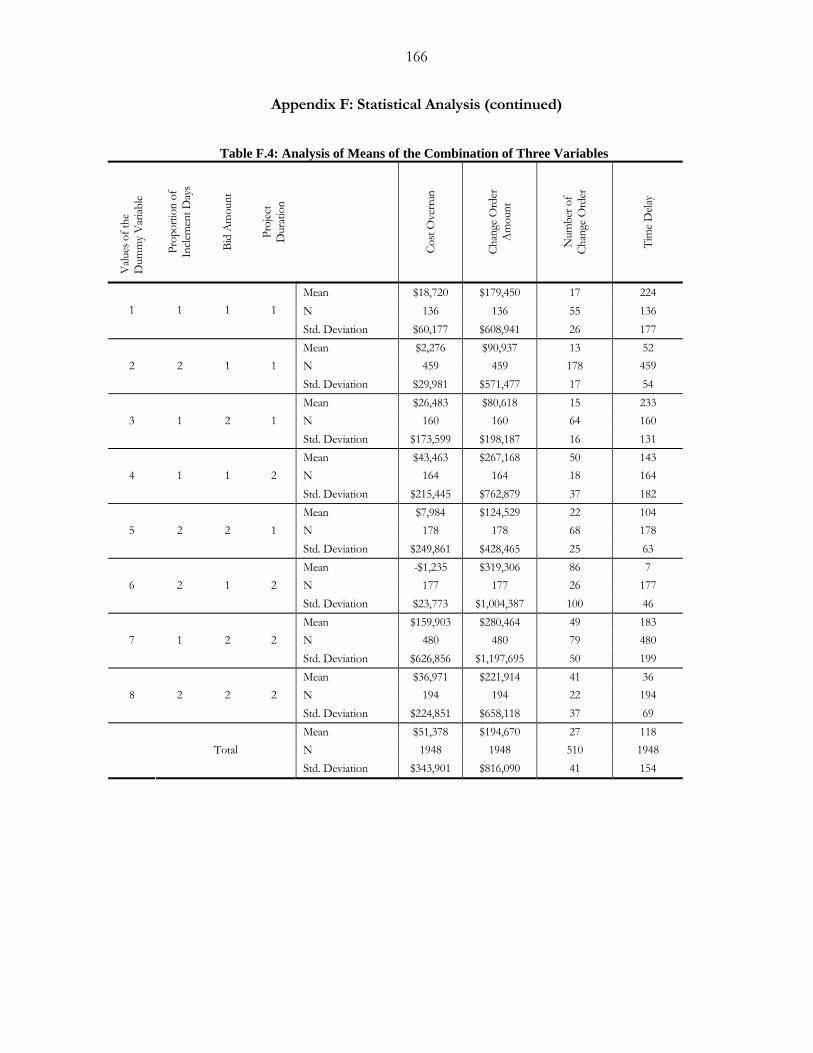
166
Appendix F: Statistical Analysis (continued)
Table F.4: Analysis of Means of the Combination of Three Variables
Valu
es o
f the
D
umm
y Var
iable
Prop
ortio
n of
In
clem
ent D
ays
Bid
Am
ount
Proj
ect
Dur
atio
n
Cost
Ove
rrun
Chan
ge O
rder
A
mou
nt
Num
ber o
f Ch
ange
Ord
er
Tim
e Dela
y
Mean $18,720 $179,450 17 224 N 136 136 55 136 1 1 1 1
Std. Deviation $60,177 $608,941 26 177 Mean $2,276 $90,937 13 52 N 459 459 178 459 2 2 1 1 Std. Deviation $29,981 $571,477 17 54 Mean $26,483 $80,618 15 233 N 160 160 64 160 3 1 2 1 Std. Deviation $173,599 $198,187 16 131 Mean $43,463 $267,168 50 143 N 164 164 18 164 4 1 1 2 Std. Deviation $215,445 $762,879 37 182 Mean $7,984 $124,529 22 104 N 178 178 68 178 5 2 2 1 Std. Deviation $249,861 $428,465 25 63 Mean -$1,235 $319,306 86 7 N 177 177 26 177 6 2 1 2 Std. Deviation $23,773 $1,004,387 100 46 Mean $159,903 $280,464 49 183 N 480 480 79 480 7 1 2 2 Std. Deviation $626,856 $1,197,695 50 199 Mean $36,971 $221,914 41 36 N 194 194 22 194 8 2 2 2 Std. Deviation $224,851 $658,118 37 69 Mean $51,378 $194,670 27 118 N 1948 1948 510 1948 Total Std. Deviation $343,901 $816,090 41 154
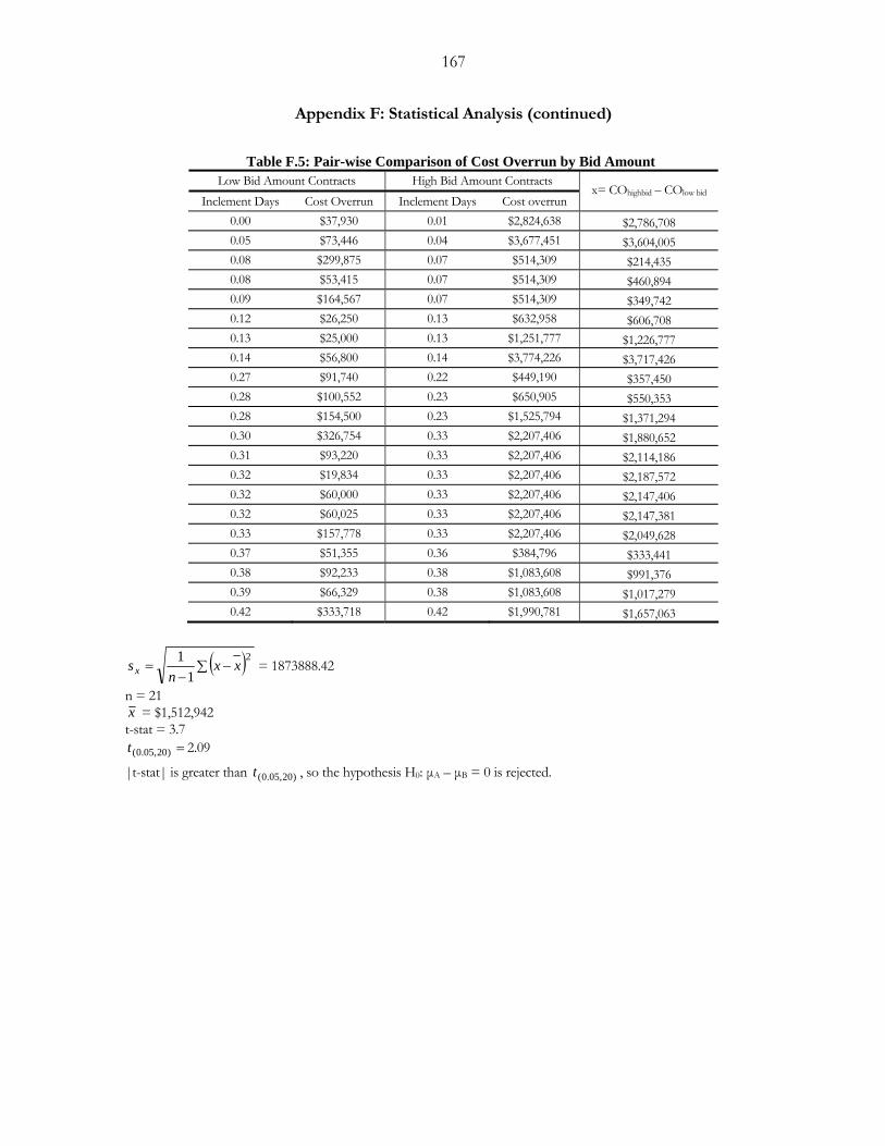
167
Appendix F: Statistical Analysis (continued)
Table F.5: Pair-wise Comparison of Cost Overrun by Bid Amount
Low Bid Amount Contracts High Bid Amount Contracts Inclement Days Cost Overrun Inclement Days Cost overrun
x= COhighbid – COlow bid
0.00 $37,930 0.01 $2,824,638 $2,786,708 0.05 $73,446 0.04 $3,677,451 $3,604,005 0.08 $299,875 0.07 $514,309 $214,435 0.08 $53,415 0.07 $514,309 $460,894 0.09 $164,567 0.07 $514,309 $349,742 0.12 $26,250 0.13 $632,958 $606,708 0.13 $25,000 0.13 $1,251,777 $1,226,777 0.14 $56,800 0.14 $3,774,226 $3,717,426 0.27 $91,740 0.22 $449,190 $357,450 0.28 $100,552 0.23 $650,905 $550,353 0.28 $154,500 0.23 $1,525,794 $1,371,294 0.30 $326,754 0.33 $2,207,406 $1,880,652 0.31 $93,220 0.33 $2,207,406 $2,114,186 0.32 $19,834 0.33 $2,207,406 $2,187,572 0.32 $60,000 0.33 $2,207,406 $2,147,406 0.32 $60,025 0.33 $2,207,406 $2,147,381 0.33 $157,778 0.33 $2,207,406 $2,049,628 0.37 $51,355 0.36 $384,796 $333,441 0.38 $92,233 0.38 $1,083,608 $991,376 0.39 $66,329 0.38 $1,083,608 $1,017,279 0.42 $333,718 0.42 $1,990,781 $1,657,063
( )∑ −−
=2
11 xx
nsx = 1873888.42
n = 21 x = $1,512,942 t-stat = 3.7
=)20,05.0(t 2.09
|t-stat| is greater than )20,05.0(t , so the hypothesis H0: µA – µB = 0 is rejected.
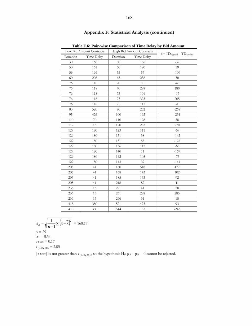
168
Appendix F: Statistical Analysis (continued)
Table F.6: Pair-wise Comparison of Time Delay by Bid Amount
Low Bid Amount Contracts High Bid Amount Contracts Duration Time Delay Duration Time Delay
x= TDhighbid – TDlow bid
30 168 30 136 -32 50 161 50 180 19 59 166 55 57 -109 60 208 65 238 30 76 118 70 70 -48 76 118 70 298 180 76 118 75 101 -17 76 118 75 323 205 76 118 75 117 -1 83 520 80 252 -268 95 426 100 192 -234 110 70 110 128 58 112 13 120 283 270 129 180 123 111 -69 129 180 131 38 -142 129 180 131 53 -127 129 180 136 112 -68 129 180 140 11 -169 129 180 142 105 -75 129 180 143 39 -141 205 41 160 518 477 205 41 168 143 102 205 41 185 133 92 205 41 218 82 41 236 13 221 41 28 236 13 261 298 285 236 13 266 31 18 418 380 521 473 93 418 380 544 137 -243
( )∑ −−
=2
11 xx
nsx = 168.17
n = 29 x = 5.34 t-stat = 0.17
=)28,05.0(t 2.05
|t-stat| is not greater than )28,05.0(t , so the hypothesis H0: µA – µB = 0 cannot be rejected.
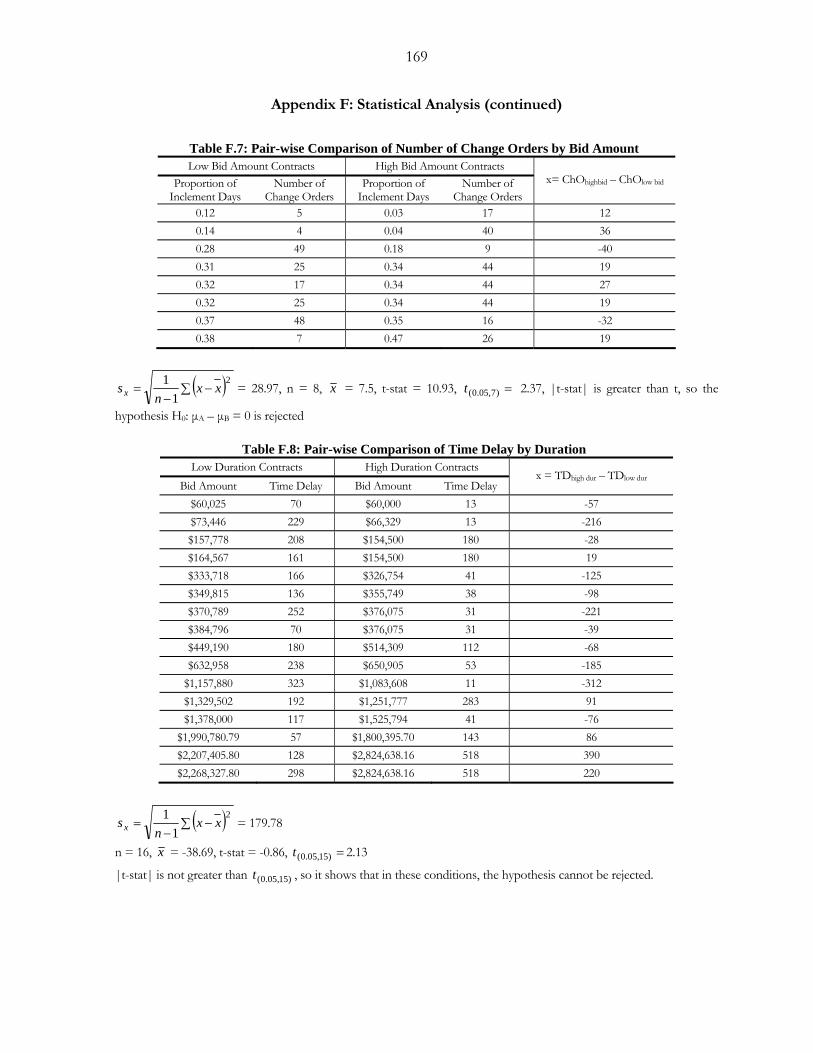
169
Appendix F: Statistical Analysis (continued)
Table F.7: Pair-wise Comparison of Number of Change Orders by Bid Amount Low Bid Amount Contracts High Bid Amount Contracts
Proportion of Inclement Days
Number of Change Orders
Proportion of Inclement Days
Number of Change Orders
x= ChOhighbid – ChOlow bid
0.12 5 0.03 17 12 0.14 4 0.04 40 36 0.28 49 0.18 9 -40 0.31 25 0.34 44 19 0.32 17 0.34 44 27 0.32 25 0.34 44 19 0.37 48 0.35 16 -32 0.38 7 0.47 26 19
( )∑ −−
=2
11 xx
nsx = 28.97, n = 8, x = 7.5, t-stat = 10.93, =)7,05.0(t 2.37, |t-stat| is greater than t, so the
hypothesis H0: µA – µB = 0 is rejected
Table F.8: Pair-wise Comparison of Time Delay by Duration Low Duration Contracts High Duration Contracts
Bid Amount Time Delay Bid Amount Time Delay x = TDhigh dur – TDlow dur
$60,025 70 $60,000 13 -57 $73,446 229 $66,329 13 -216 $157,778 208 $154,500 180 -28 $164,567 161 $154,500 180 19 $333,718 166 $326,754 41 -125 $349,815 136 $355,749 38 -98 $370,789 252 $376,075 31 -221 $384,796 70 $376,075 31 -39 $449,190 180 $514,309 112 -68 $632,958 238 $650,905 53 -185
$1,157,880 323 $1,083,608 11 -312 $1,329,502 192 $1,251,777 283 91 $1,378,000 117 $1,525,794 41 -76
$1,990,780.79 57 $1,800,395.70 143 86 $2,207,405.80 128 $2,824,638.16 518 390 $2,268,327.80 298 $2,824,638.16 518 220
( )∑ −−
=2
11 xx
nsx = 179.78
n = 16, x = -38.69, t-stat = -0.86, =)15,05.0(t 2.13
|t-stat| is not greater than )15,05.0(t , so it shows that in these conditions, the hypothesis cannot be rejected.
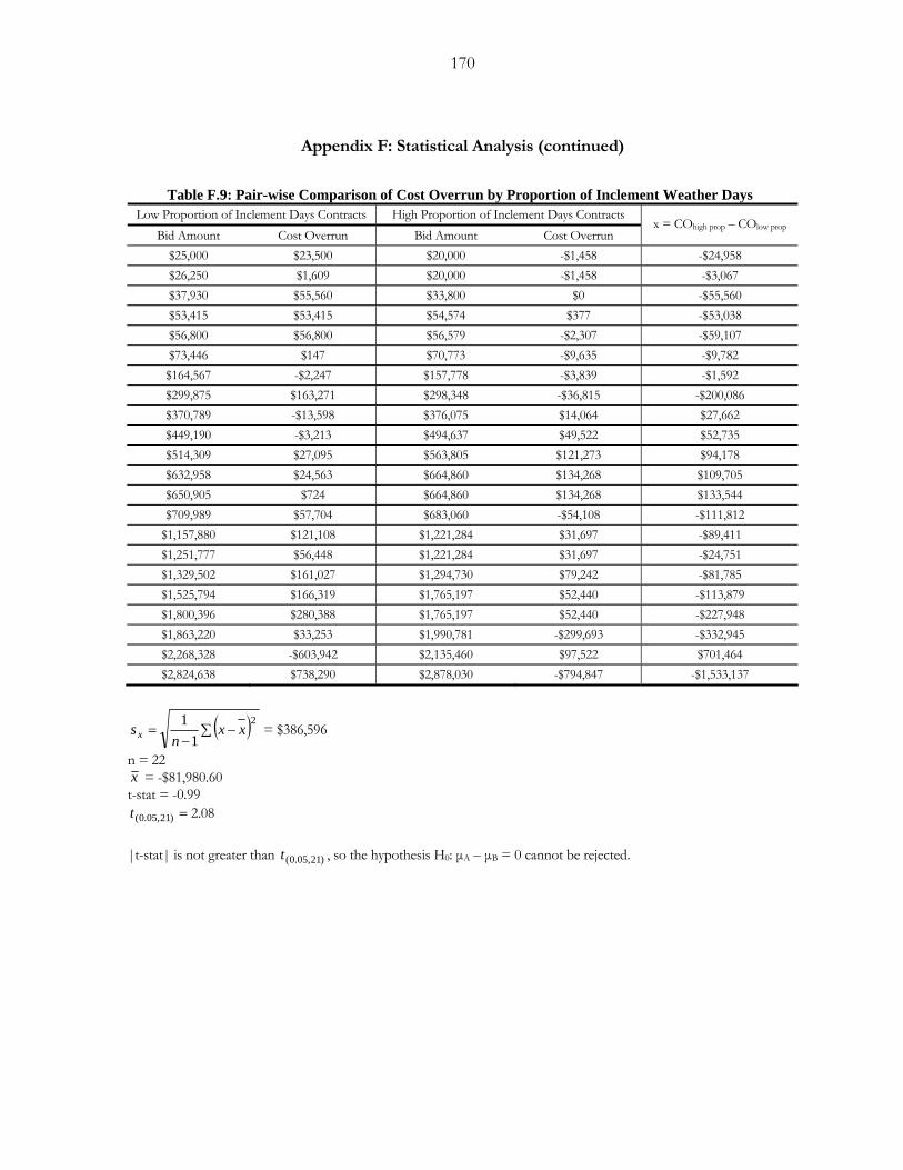
170
Appendix F: Statistical Analysis (continued)
Table F.9: Pair-wise Comparison of Cost Overrun by Proportion of Inclement Weather Days
Low Proportion of Inclement Days Contracts High Proportion of Inclement Days Contracts Bid Amount Cost Overrun Bid Amount Cost Overrun
x = COhigh prop – COlow prop
$25,000 $23,500 $20,000 -$1,458 -$24,958 $26,250 $1,609 $20,000 -$1,458 -$3,067 $37,930 $55,560 $33,800 $0 -$55,560 $53,415 $53,415 $54,574 $377 -$53,038 $56,800 $56,800 $56,579 -$2,307 -$59,107 $73,446 $147 $70,773 -$9,635 -$9,782 $164,567 -$2,247 $157,778 -$3,839 -$1,592 $299,875 $163,271 $298,348 -$36,815 -$200,086 $370,789 -$13,598 $376,075 $14,064 $27,662 $449,190 -$3,213 $494,637 $49,522 $52,735 $514,309 $27,095 $563,805 $121,273 $94,178 $632,958 $24,563 $664,860 $134,268 $109,705 $650,905 $724 $664,860 $134,268 $133,544 $709,989 $57,704 $683,060 -$54,108 -$111,812
$1,157,880 $121,108 $1,221,284 $31,697 -$89,411 $1,251,777 $56,448 $1,221,284 $31,697 -$24,751 $1,329,502 $161,027 $1,294,730 $79,242 -$81,785 $1,525,794 $166,319 $1,765,197 $52,440 -$113,879 $1,800,396 $280,388 $1,765,197 $52,440 -$227,948 $1,863,220 $33,253 $1,990,781 -$299,693 -$332,945 $2,268,328 -$603,942 $2,135,460 $97,522 $701,464 $2,824,638 $738,290 $2,878,030 -$794,847 -$1,533,137
( )∑ −−
=2
11 xx
nsx = $386,596
n = 22 x = -$81,980.60 t-stat = -0.99
=)21,05.0(t 2.08 |t-stat| is not greater than )21,05.0(t , so the hypothesis H0: µA – µB = 0 cannot be rejected.
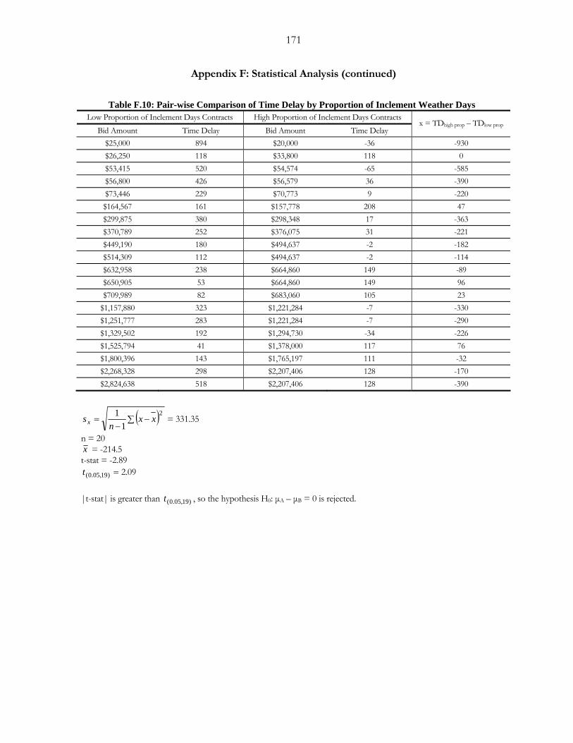
171
Appendix F: Statistical Analysis (continued)
Table F.10: Pair-wise Comparison of Time Delay by Proportion of Inclement Weather Days
Low Proportion of Inclement Days Contracts High Proportion of Inclement Days Contracts Bid Amount Time Delay Bid Amount Time Delay
x = TDhigh prop – TDlow prop
$25,000 894 $20,000 -36 -930 $26,250 118 $33,800 118 0 $53,415 520 $54,574 -65 -585 $56,800 426 $56,579 36 -390 $73,446 229 $70,773 9 -220 $164,567 161 $157,778 208 47 $299,875 380 $298,348 17 -363 $370,789 252 $376,075 31 -221 $449,190 180 $494,637 -2 -182 $514,309 112 $494,637 -2 -114 $632,958 238 $664,860 149 -89 $650,905 53 $664,860 149 96 $709,989 82 $683,060 105 23
$1,157,880 323 $1,221,284 -7 -330 $1,251,777 283 $1,221,284 -7 -290 $1,329,502 192 $1,294,730 -34 -226 $1,525,794 41 $1,378,000 117 76 $1,800,396 143 $1,765,197 111 -32 $2,268,328 298 $2,207,406 128 -170 $2,824,638 518 $2,207,406 128 -390
( )∑ −−
=2
11 xx
nsx = 331.35
n = 20 x = -214.5 t-stat = -2.89
=)19,05.0(t 2.09 |t-stat| is greater than )19,05.0(t , so the hypothesis H0: µA – µB = 0 is rejected.
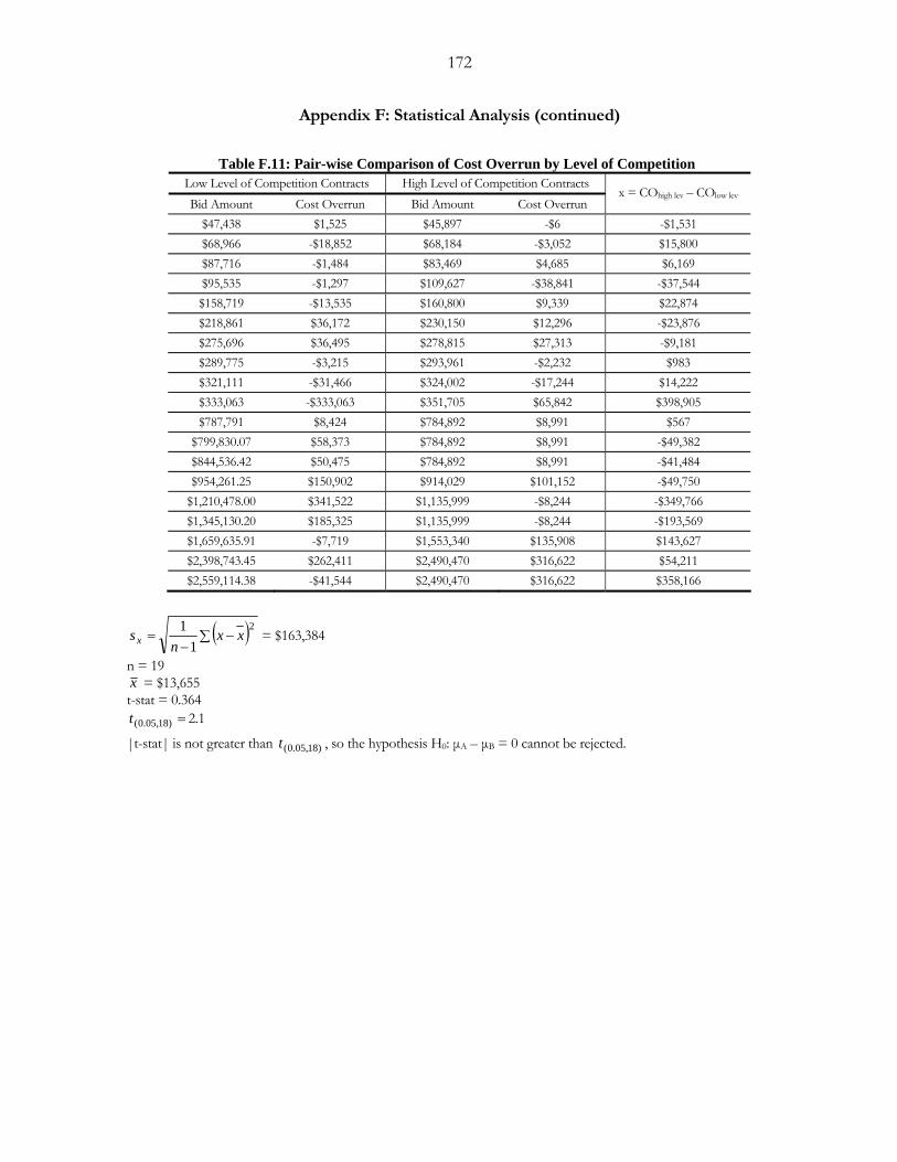
172
Appendix F: Statistical Analysis (continued)
Table F.11: Pair-wise Comparison of Cost Overrun by Level of Competition
Low Level of Competition Contracts High Level of Competition Contracts Bid Amount Cost Overrun Bid Amount Cost Overrun
x = COhigh lev – COlow lev
$47,438 $1,525 $45,897 -$6 -$1,531 $68,966 -$18,852 $68,184 -$3,052 $15,800 $87,716 -$1,484 $83,469 $4,685 $6,169 $95,535 -$1,297 $109,627 -$38,841 -$37,544 $158,719 -$13,535 $160,800 $9,339 $22,874 $218,861 $36,172 $230,150 $12,296 -$23,876 $275,696 $36,495 $278,815 $27,313 -$9,181 $289,775 -$3,215 $293,961 -$2,232 $983 $321,111 -$31,466 $324,002 -$17,244 $14,222 $333,063 -$333,063 $351,705 $65,842 $398,905 $787,791 $8,424 $784,892 $8,991 $567
$799,830.07 $58,373 $784,892 $8,991 -$49,382 $844,536.42 $50,475 $784,892 $8,991 -$41,484 $954,261.25 $150,902 $914,029 $101,152 -$49,750
$1,210,478.00 $341,522 $1,135,999 -$8,244 -$349,766 $1,345,130.20 $185,325 $1,135,999 -$8,244 -$193,569 $1,659,635.91 -$7,719 $1,553,340 $135,908 $143,627 $2,398,743.45 $262,411 $2,490,470 $316,622 $54,211 $2,559,114.38 -$41,544 $2,490,470 $316,622 $358,166
( )∑ −−
=2
11 xx
nsx = $163,384
n = 19 x = $13,655 t-stat = 0.364
=)18,05.0(t 2.1
|t-stat| is not greater than )18,05.0(t , so the hypothesis H0: µA – µB = 0 cannot be rejected.
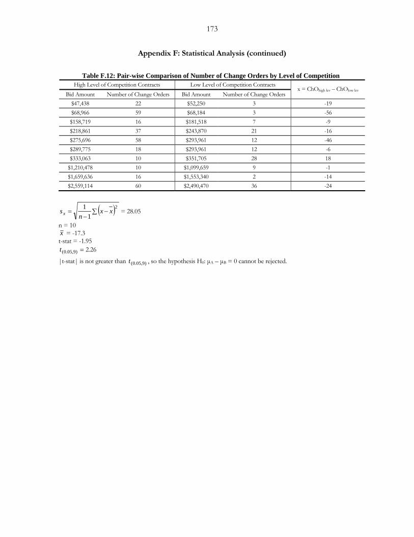
173
Appendix F: Statistical Analysis (continued)
Table F.12: Pair-wise Comparison of Number of Change Orders by Level of Competition
High Level of Competition Contracts Low Level of Competition Contracts Bid Amount Number of Change Orders Bid Amount Number of Change Orders
x = ChOhigh lev – ChOlow lev
$47,438 22 $52,250 3 -19 $68,966 59 $68,184 3 -56 $158,719 16 $181,518 7 -9 $218,861 37 $243,870 21 -16 $275,696 58 $293,961 12 -46 $289,775 18 $293,961 12 -6 $333,063 10 $351,705 28 18
$1,210,478 10 $1,099,659 9 -1 $1,659,636 16 $1,553,340 2 -14 $2,559,114 60 $2,490,470 36 -24
( )∑ −−
=2
11 xx
nsx = 28.05
n = 10 x = -17.3 t-stat = -1.95
=)9,05.0(t 2.26
|t-stat| is not greater than )9,05.0(t , so the hypothesis H0: µA – µB = 0 cannot be rejected.
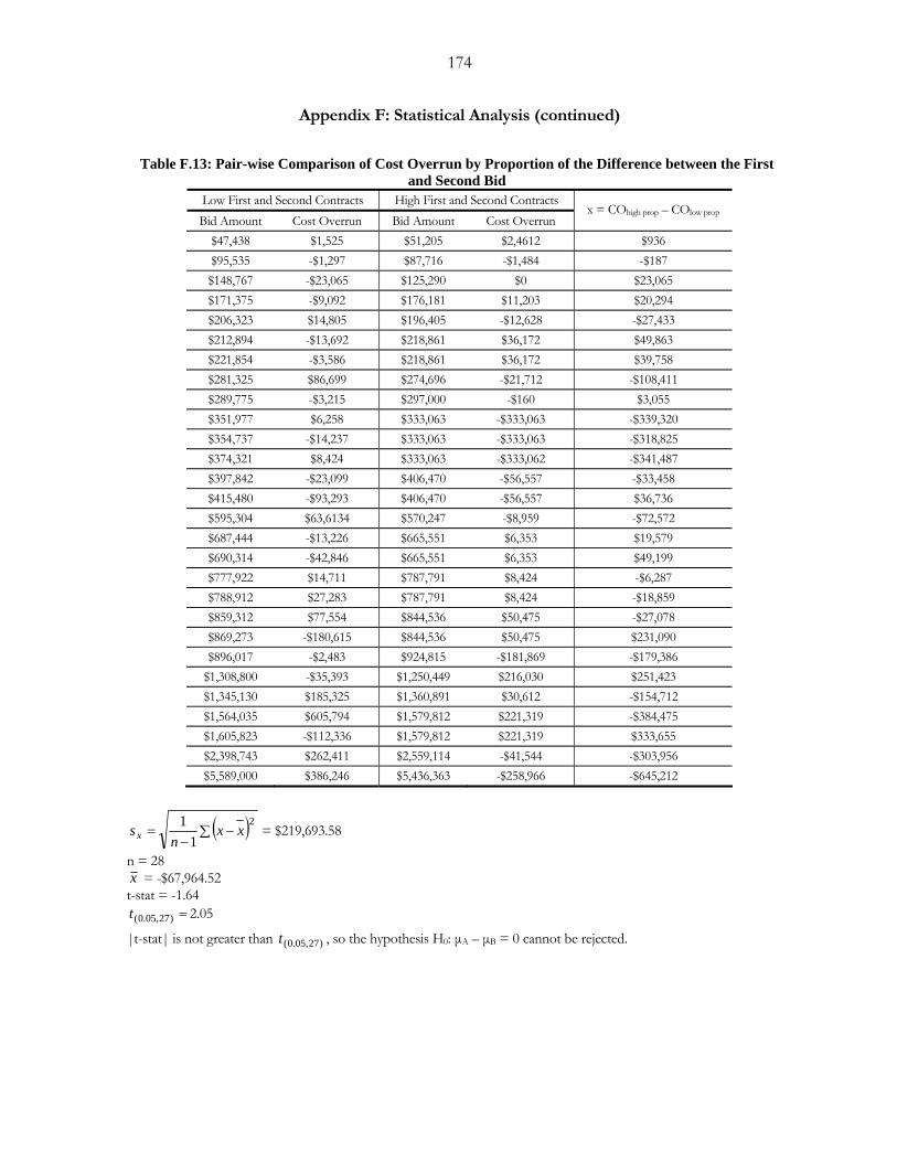
174
Appendix F: Statistical Analysis (continued)
Table F.13: Pair-wise Comparison of Cost Overrun by Proportion of the Difference between the First
and Second Bid Low First and Second Contracts High First and Second Contracts Bid Amount Cost Overrun Bid Amount Cost Overrun
x = COhigh prop – COlow prop
$47,438 $1,525 $51,205 $2,4612 $936 $95,535 -$1,297 $87,716 -$1,484 -$187 $148,767 -$23,065 $125,290 $0 $23,065 $171,375 -$9,092 $176,181 $11,203 $20,294 $206,323 $14,805 $196,405 -$12,628 -$27,433 $212,894 -$13,692 $218,861 $36,172 $49,863 $221,854 -$3,586 $218,861 $36,172 $39,758 $281,325 $86,699 $274,696 -$21,712 -$108,411 $289,775 -$3,215 $297,000 -$160 $3,055 $351,977 $6,258 $333,063 -$333,063 -$339,320 $354,737 -$14,237 $333,063 -$333,063 -$318,825 $374,321 $8,424 $333,063 -$333,062 -$341,487 $397,842 -$23,099 $406,470 -$56,557 -$33,458 $415,480 -$93,293 $406,470 -$56,557 $36,736 $595,304 $63,6134 $570,247 -$8,959 -$72,572 $687,444 -$13,226 $665,551 $6,353 $19,579 $690,314 -$42,846 $665,551 $6,353 $49,199 $777,922 $14,711 $787,791 $8,424 -$6,287 $788,912 $27,283 $787,791 $8,424 -$18,859 $859,312 $77,554 $844,536 $50,475 -$27,078 $869,273 -$180,615 $844,536 $50,475 $231,090 $896,017 -$2,483 $924,815 -$181,869 -$179,386
$1,308,800 -$35,393 $1,250,449 $216,030 $251,423 $1,345,130 $185,325 $1,360,891 $30,612 -$154,712 $1,564,035 $605,794 $1,579,812 $221,319 -$384,475 $1,605,823 -$112,336 $1,579,812 $221,319 $333,655 $2,398,743 $262,411 $2,559,114 -$41,544 -$303,956 $5,589,000 $386,246 $5,436,363 -$258,966 -$645,212
( )∑ −−
=2
11 xx
nsx = $219,693.58
n = 28 x = -$67,964.52 t-stat = -1.64
=)27,05.0(t 2.05
|t-stat| is not greater than )27,05.0(t , so the hypothesis H0: µA – µB = 0 cannot be rejected.
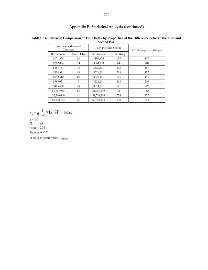
175
Appendix F: Statistical Analysis (continued)
Table F.14: Pair-wise Comparison of Time Delay by Proportion of the Difference between the First and
Second Bid Low First and Second
Contracts High First and Second
Bid Amount Time Delay Bid Amount Time Delay x = TDhigh prop – TDlow prop
$171,375 50 $196,405 197 147 $212,894 74 $264,778 64 -10 $354,737 16 $321,111 215 199 $374,321 18 $321,111 215 197 $382,510 60 $321,111 215 155 $385,051 7 $321,111 215 208 $415,480 59 $514,001 30 -29
$1,564,035 66 $1,250,449 54 -12 $2,246,000 101 $2,559,114 378 277 $2,398,743 25 $2,559,114 378 353
( )∑ −−
=2
11 xx
nsx = 202.69
n = 10 x = 148.5 t-stat = 2.32
=)9,05.0(t 2.26
|t-stat| is greater than )9,05.0(t
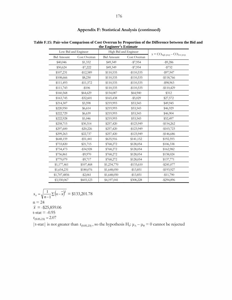
176
Appendix F: Statistical Analysis (continued)
Table F.15: Pair-wise Comparison of Cost Overrun by Proportion of the Difference between the Bid and
the Engineer’s Estimate Low Bid and Engineer High Bid and Engineer
Bid Amount Cost Overrun Bid Amount Cost Overrun x = COhigh prop – COlow prop
$40,046 $1,332 $49,349 -$7,954 -$9,286 $50,624 -$7,222 $49,349 -$7,954 -$732 $107,231 -$12,589 $110,535 -$110,535 -$97,947 $108,666 $8,230 $110,535 -$110,535 -$118,766 $111,493 -$11,572 $110,535 -$110,535 -$98,963 $111,743 -$106 $110,535 -$110,535 -$110,429 $160,568 $64,629 $154,087 $64,940 $312 $163,745 -$32,601 $165,438 -$5,029 $27,572 $214,307 $3,598 $219,993 $53,543 $49,945 $220,950 $6,614 $219,993 $53,543 $46,929 $222,729 $6,639 $219,993 $53,543 $46,904 $222,928 $1,046 $219,993 $53,543 $52,497 $258,715 $30,314 $257,420 -$123,949 -$154,262 $297,600 -$20,226 $257,420 -$123,949 -$103,723 $299,263 $22,737 $257,420 -$123,949 -$146,686 $648,159 -$51,441 $635,916 $141,152 $192,593 $733,820 $21,715 $768,272 $128,054 $106,338 $734,473 -$34,928 $768,272 $128,054 $162,982 $756,861 -$9,970 $768,272 $128,054 $138,024 $779,079 -$9,717 $768,272 $128,054 $137,771
$1,177,461 $107,468 $1,234,770 -$133,610 -$241,077 $1,654,231 $180,076 $1,648,050 -$13,851 -$193,927 $1,707,4856 -$2,061 $1,648,050 -$13,851 -$11,790 $3,550,067 $603,123 $4,197,041 $308,228 -$294,896
( )∑ −−
=2
11 xx
nsx = $133,201.78
n = 24 x = -$25,859.06 t-stat = -0.95
=)23,05.0(t 2.07 |t-stat| is not greater than )23,05.0(t , so the hypothesis H0: µA – µB = 0 cannot be rejected
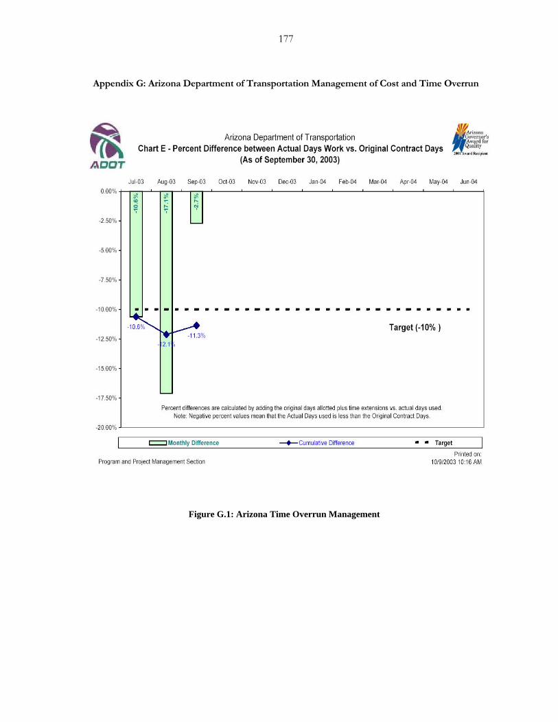
177
Appendix G: Arizona Department of Transportation Management of Cost and Time Overrun
Figure G.1: Arizona Time Overrun Management
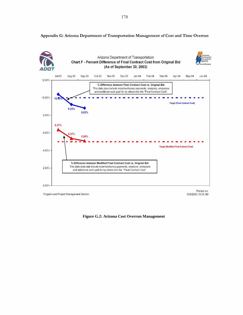
178
Appendix G: Arizona Department of Transportation Management of Cost and Time Overrun
Figure G.2: Arizona Cost Overrun Management