An Alternative Theory of the Plant Size Distributionwith an Application to Trade

by

Thomas J. Holmes and John J. Stevens1

April 2009

Note: This is a preliminary and incomplete draft for seminar presentation

1Holmes: University of Minnesota, Federal Reserve Bank of Minneapolis, and NBER. Stevens: The

Board of Governors of the Federal Reserve System. The views expressed herein are solely those of the

authors and do not represent the views of the Federal Reserve Banks of Minneapolis, the Federal Reserve

System, or the U.S. Bureau of the Census. The research presented here was funded by NSF grant SES

0551062. We thank Steve Schmeiser and Julia Thornton for their research assistance for this project. We

thank Shawn Klimek for his help with the Census Micro Data. The statistics reported in this paper derived

from Census micro data were screened to ensure that they do not disclose confidential information.

1 Introduction

There is wide variation in the sizes of manufacturing plants, even within the most narrowly-

defined industry classifications used by statistical agencies. For example, in the wood

furniture industry in the United States (NAICS industry code 337122), one can find plants

with over a thousand employees and other plants with as few as one or two employees. The

dominant theory of within-industry size differentials, like these, models plants as varying in

terms of productivity. See Lucas (1978), Jovanovic (1982), and Hopenhayn (1992). In

this theory, some plants are lucky and obtain high productivity draws when they enter an

industry. Others are unlucky and obtain low productivity draws. The size distribution is

driven entirely by the productivity distribution.

The approach has been extremely influential. It underpins recent developments in the

international trade literature. Melitz (2003) and Eaton and Kortum (2002) use the approach

to explain plant-level trade facts. In Melitz, plants with higher productivity draws have large

domestic sales and also have the incentive to pay fixed costs to enter export markets. In this

way, the Melitz model explains the fact–documented by Bernard and Jensen (1995)–that

large plants within narrowly-defined industries are more likely to be exporters than small

plants. Relatedly, in Eaton and Kortum, more productive plants have wider trade areas.

Both the Melitz and the Eaton and Kortum theories have a sharp implication about how

increased exposure to import competition impacts a domestic industry. The smaller plants

in the industry–which are the low productivity plants in the industry–are the first to exit.

This approach is influential as well in the macroeconomics literature on quantitative dy-

namic models incorporating plant heterogeneity. Given a monotonic relationship between

plant size and productivity, it is possible to invert the relationship and read off the distrib-

ution of plant productivities from the distribution of plant sizes. Hopenhayn and Rogerson

(1993) is an early example; Atkeson and Kehoe (2005) a recent example.

In our view, the existing literature has gone too far in attributing all differences in plant

size within narrowly-defined Census industries to differences in productivity. It is likely

that plants that are dramatically different in size are doing different things, even if the

Census happens to put them in the same industry. Moreover, these differences are likely

to be systematic; we expect small manufacturing plants to specialize in provide custom and

retail-like services in a way that large plants classified in the same Census industry do not.

Systematic differences like these have major implications for determining the relative impact

of increased import pressure.

1

Take wood furniture, for example. The large plants in this industry with more than

1,000 employees are concentrated in North Carolina. These plants make the stock kitchen

and bedroom furniture pieces one finds at traditional furniture stores. Also included in the

Census classification are small facilities making custom pieces to order, such as small shops

employing Amish skilled craftsman. Let us apply the standard theory of the size distribution

to this industry. Entrepreneurs entering and drawing a high productivity parameter open

up megaplants in North Carolina; those with low draws perhaps open Amish shops. The

Melitz model and the Eaton Kortum model both predict the large North Carolina plants

will have large market areas, while the small plants will tend to ship locally. So far so

good, because this is consistent with the data as we show below. But what happens when

China enters the wood furniture market in a dramatic fashion as has occurred over the past

ten years? While all of the U.S. industry will be hurt, the Melitz and Eaton and Kortum

theories predict the North Carolina industry will be relatively less impacted because it is

home to the large, productive plants. In fact the opposite turned out to be true.

Our theory takes into account that typically in any industry that tends to be some

segment providing custom services that are facilitated by face-to-face contact between buyers

and sellers. This nontradable segment is the province of small plants. When China enters

the wood furniture market, it naturally enters the tradable segment of the market, which

happens to be the stock pieces that the large plants in North Carolina make. In this theory,

the North Carolina industry is hurt the most, as actually happened.

Our model highlights the role of geography within a domestic market. The model is

estimated separately for individual industries using Census data that includes information

on the origins and destinations of shipments (the Commodity Flow Survey or CFS). The

estimated model is put to work examining two quantitative issues. The first concerns the

relationship between the geographic distribution of an industry and its size distribution. In

the data, plants in an industry tend to be significantly larger at locations where an industry

concentrates. The second concerns the impact of a trade shock. For both quantitative

exercises, our estimated model that allows for a nontradable segment does well. When we

follow the standard approach and do not allow for the nontradable segment, the results are

poor.

Our starting point is the Eaton and Kortum (2002) model of geography and trade as

further developed in Bernard, Eaton, Jensen, and Kortum (2003) (BEJK). In its basic form,

plants vary in productivity and location, but are otherwise symmetric in terms of trans-

portation costs and underlying consumer demand. We take their model “off the shelf”

2

as our model of the tradable segment of an industry, and we fold in a simple model of a

nontradable segment. We then explore the implications of this theory for facts about geo-

graphic dispersion of production and what average plant size looks like at locations where

an industry concentrates. A key result of our analysis is that for the tradable segment,

when transportation costs are not very big, average plant size in regions where the industry

concentrates will not be much bigger than average plant size in the tradable segment overall.

Put in another way, when transportation costs are not too big, most of the expansion in

production in such locations is accommodated on the extensive margin of an increased count

in the number of plants rather then the intensive margin of larger average plant size. The

discipline in our analysis comes from the information we use about shipping distances. The

essence of our empirical finding is that for most industries, the tradable segment plants are

shipping relatively long distances, and from this we infer that transportation costs for the

tradable segments cannot be very big. Hence, the average plant size differences across loca-

tions should be relatively small. So the BEJK model on its own–without the nontradable

segment that we incorporate–is incapable of accounting of the wide swings in average plant

size across locations that is actually observed.

Before we get to the business of estimating our model, as a first step we derive a set of

descriptive statistics related to the implications of the theory. We take populations of plants

and consider various ways of classifying plants as either being in tradable and nontradable

segments. We show that regardless of the way we do it, compared to tradables, nontradable

plants:

• are smaller,

• are more geographically dispersed,

• have higher plant counts,

• are less likely to export,

• are less likely to ship goods long distances within the United States.

Some of these findings replicated earlier results by Bernard and Jensen (1995) and Holmes

and Stevens (2002) and some are new. We start by showing these patterns hold when

we classify all manufacturing plants as tradable and all retail plants as nontradable. This

should surprise no one; obviously retail plants are geographically disperse, cater to local

consumers, and are numerous and small, as compared to manufacturing plants. Things

3

get more interesting when we look within manufacturing. We look across six-digit NAICS

industries (the finest level of detail) within manufacturing and show the patterns hold when

we treat industries like “Quick Printing" and “Ice” as nontradable. Once we see that the

same patterns occurring across manufacturing and retail can be found within manufacturing

across six-digit NAICS industries, it is natural to take the next step and see if analogous

patterns occur within six-digit industries. We approach this step in two ways. First, we

exploit information in the 1997 Census conversion from the SIC system to the NAICS system

to arrive at a nontradable/tradable distinction for eight industries. Second, we use plant

size to determine tradable/nontradable status. The patterns described above hold either

way. Within narrowly defined manufacturing industries, we see the same patterns that we

find in comparisons across manufacturing and retail. A small hand-crafted furniture plant,

grouped in the same classification as a gigantic North Carolina factory, may have more in

common with a retail shop.

2 Theory

The first part of this section presents the model. The second part derives analytic results.

2.1 Model

We develop a model of a manufacturing industry with two segments, a tradable (or )

segment that makes goods that can be transported across space and a nontradable (or )

segment that makes custom goods. There is a fixed set of locations, indexed by .

For simplicity we take total spending on the industry at each location to be exogenous

at . Moreover, the share of spending on the tradable and nontradable segments is fixed

at and , + = 1. Spending on the two segments at location is then

=

=

2.1.1 The Tradable Segment

We use the BEJK model as our model of the tradable segment. There is a continuum

of differentiated goods indexed by ∈ [0 1]. These goods are aggregated to obtain a

4

tradable segment composite good for the industry in the standard constant-elasticity-of-

substitution way. Let () be the price of good at location . (For simplicity we leave

the “” superscript implicit here as the index only refers to tradable goods.) Then the

expenditure at location for good equals

() =

µ()

¶1−

where is the price index for the tradable segment composite at location ,

=

∙Z 1

0

()1−

¸ 11−

As in BEJK, there are potential producers at each location with varying levels of technical

efficiency. Let () index the efficiency of the th most efficient producer of good located

at . This index represents the amount of good made by this producer, per unit of input.

There is an “iceberg” cost to ship tradable segment goods across locations. Let be

the amount of good that must be shipped to location from location in order to deliver

one unit. Now = 1, so there is no transportation cost for delivering to the location where

the good is produced. Otherwise, ≥ 1, for 6= . Assume that the triangle inequality

≤ holds.

The distribution of efficiencies are determined as follows. Let denote the wage at

location , and let denote a parameter governing the distribution of efficiency of the

tradable segment at location . Suppose the maximum efficiency 1 is drawn according to

() = −−.

The parameter governs the variance of productivity draws.

Eaton and Kortum (2002) show that for a given tradable segment good , the probability

location is the lowest cost producer to location is

=P

=1 , (1)

5

for

≡ −

= ()−.

We refer to as the efficiency index for location and as the transportation structure

between and . Let Γ = (1 2 ) be the efficiency vector and (with elements ) be

the transportation structure matrix These terms are an abuse of terminology because these

are not the structural parameters of the model, but are rather reduced form parameters,

as we see above. Nevertheless, these parameters summarize the information content of the

BEJK model in our data and these are the parameters we will estimate. For the exercises

we will consider, estimates of these reduced form parameters is sufficient.

BEJK consider a rich structure with multiple potential producers at each location who

each get their own productivity draw. Then firms engage in Bertrand competition for con-

sumers at each location. The equilibrium may feature limit pricing, where the lowest cost

producer matches the second lowest cost. Or the lowest cost may be so low relative to rivals’

costs that the price is determined by the inverse elasticity rule for the optimal monopoly

price. The remarkable result of BEJK is that allowing for all of this does not matter. Con-

ditional on a location landing a sale at (i.e. that location is the low cost producer for ),

the distribution of prices to is the same for all . This implies that the sales revenues from

are allocated according to . That is, total sales revenue from location from tradable

segment goods originating at is

= .

Total sales revenues on tradable segment goods originating in across all destinations is

=

X=1

.

We associate a plant with a particular good produced at . The measure of goods

produced at equals , the measure of goods location sells to itself. (On account of the

triangle inequality ≤ , if a particular plant is the most efficient producer at any

location, it is also the most efficient producer at its own location.) We also allow for a scaling

factor , so that the number (more formally the measure) of plants in the tradable segment

6

at location is

= (2)

2.1.2 The Nontradable Segment

The nontradable segment is modeled in a very simple fashion. First, since the segment is

nontradable, total sales of plants located in equals local demand, i.e.

= .

Second, we assume that there is an efficient plant sales size equal to . So the number of

plants in the nontradable segment at is

=

=

= . (3)

for

≡

.

The parameter is the number (measure) of nontradable plants per unit of demand. Since

the are scaled to sum to one, is the number of nontradable plants across the entire

economy.

Note that the nontradable segment differs from the tradable segment in two substantive

ways. The first is that tradables can be shipped. The second difference applies even for

goods sold locally. In the tradable segment, only one plant produces a given good . So if

a given plant at is producing good , and if demand increases at location , everything else

the same, the plant producing good sells more, and there is no entry of new plants. Thus

for tradables, an increase in local spending (holding the distribution of productivities fixed)

is accommodated at the intensive margin, with existing plants producing more. In contrast,

in the nontradable sector, an increase in demand is accommodated at the extensive margin

with more plants.

2.2 Results

This subsection develops drives analytic results that complement our subsequent empirical

analysis. Here we develop qualitative results related to the two main topics of interest in

7

this paper: (1) how geographic concentration of industry relates to average plant size and

(2) how imports impact the plant size distribution.

To make things tractable, for our analytic results we focus on the following special case

of the model::

The Constant-Transportation Cost, Unit Elasticity Special Case (CT-UE). This hold

when (i) = ≤ 1, for all 6= (so the transportation costs for each location pair is the

same) and (ii) = 1 (unit elasticity of demand).

The measure of size we use in the results is sales. Recall from above that average plant

size in the nontradable segment is a parameter . For the tradable segment, average plant

size is endogenous and in general varies across locations. At location it equals

=

and at the aggregate level across all locations it equals

=

=

P

=1 P

=1

.

(Note that when we leave out the location subscript , it signifies the variable is evaluated

at the aggregate level across all locations.) Regarding average size across the segments, we

assume that (a parameter) is less than the endogenous average traded good size .

2.2.1 Geographic Concentration

Our first set of results concern geographic concentration. We begin by defining a measure of

geographic concentration. Let index a group of plants (e.g. = if the group is all plants

selling a tradable segment good). For group , define the location quotient at location to

be

≡

. (4)

As typically defined in the regional economics literature, the location quotient is the fraction

of group sales that originate at location divided by location ’s share of demand. A

focal case here is when = 1 and a location’s share of sales equals its share of demand.

If 1, the location specializes in activity as compared with its demand level. Next

8

define to be the weighted average of the location quotients across all locations

=

P

P

=X

(

)2

. (5)

We will refer to this as the industry mean location quotient. Note that it is the standard

Herfindahl index of the distribution of sales across locations, with an additional term

in the denominator to make an adjustment for differences in demand across locations. It

is straightforward to derive that the lower bound of this measure is = 1 and that this

happens only when = 1 everywhere. An immediate consequence of this is

Proposition 1. ≥ = 1.

By assumption, the nontradable segment exactly follows population so of course

exactly equals one. For the traded sector, in general, a location’s share of production will

be different than it’s share of demand and so is above one. So the nontradable segment

is both smaller on average and more geographically diffuse than the tradable segment.

Next we examine the link between average plant size and geographic concentration across

locations within the tradable segment. We start by looking at the limiting case where

transportation costs are zero. For this special case we have:

Proposition 2. If = 1 all 6= , then = all .

Proof. When there is no transportation cost, the lowest cost producer for a given good

serves all the markets for this good. In this limiting case, the probability (1) that a given

location is the low cost producer for a given good reduces to P

. This ratio equals

the fraction of plants located at and it also equals the share of sales originating at . It is

immediate that average sales per plant must be the same at each location. Q.E.D.

In the limiting case with no transportation costs, the establishment count and sales at

a location are governed by how the efficiency parameter of location compares to the

other locations. A location with higher has more sales, but all of the expansion takes

place on average at the extensive margin with more plants, as average plant size stays the

same.

With positive transportation costs, the intensive margin comes into play. Locations

where the industry concentrates have larger plants on average. To highlight the issues, as

in Holmes and Stevens (2002) we decompose the sales location quotient defined earlier in (4)

9

as the product of two components

≡

(6)

=

×

(7)

=

×

(8)

= ×

. (9)

(Note, henceforth we use the superscript “sales” to distinguish the various quotients. If there

is no superscript, the sales quotient should be understood.) The first component is

the count quotient ; this is how the location’s share of plant counts compares with its share

of demand. The second is the size quotient , the average size at the location compare

to the aggregate average size. If 1 so location specializes in the industry on the

basis of sales, then location tends to have a relatively higher plant count ( 1) or

larger plants ( 1) compared with the economy as a whole, or both factors may come

into play.

Our main finding is that most of the action in the BEJK model comes through the count

(extensive) margin. We make this point for the = 2 case. Let ∈ [0 1] denote thetransportation structure between the two locations with = 1 for zero transportation costs

and = 0 for infinite costs. With only two locations, if we know the sales quotient 2 and

we are given and the demands 1 and 2, we can back out the ratio 21 that results in

this 2 . Then with the model parameters we can calculate the corresponding

2 and

2 . We do this exercise in Table 1 going through various combinations of parameters that

would result in 2 = 4, i.e. when sales are disproportionately concentrated in location

2 by a factor of 4. The table considers what happens with a wide range of and three

different cases for local demand. In the first case, the locations are equal in size (1 = 2),

in the second, location 2 is larger (2 = 31), and in the third, location 1 is larger (1 = 32).

We start by discussing the equal size case. Note that as is decreased (so that transporta-

tion costs are bigger), the productivity advantage of location 2 (21) must be increased

to hold constant the trade between the two locations (i.e. 2 = 4). At the limiting case

where = 1, we know from Proposition 2 that average size is the same in both places; i.e.,

2 = 1 as reported in the table. For this limiting case, the expansion in sales at location

2 comes entirely from the count margin, 2 =

2 . As is decreased, average size in

10

location 2 increases, so both the size margin and the establishment margin play a role. But

even as gets small, the establishment margin is always greater than the size margin. This

holds more generally in other numerical examples with 1 = 2.

When transportation cost is zero, it doesn’t matter if locations differ in demand; average

plant size is the same across all locations. But when transportation cost matter, differences

in local demand affect average plant size in the obvious way: locations with more demand

have larger plants. In particular, in the case where location 2 is larger, the size margin

eventually outweighs the establishment margin for high enough transportation costs ( less

than or equal to .5). The interesting point is that transportation costs have to be quite

substantial for this to happen. A discussion of magnitudes awaits our quantitative analysis

later in the paper. But Table 1 is a preview of the difficulties that the straight Eaton-

Kortum model has in simultaneously generating a high degree of trade between locations

and large differences in average plant size across locations.

2.2.2 Response to an External Trade Shock

Our second set of results concern how the plant distribution is impacted by a trade shock.

The experiment we consider is what happens when an foreign location becomes more produc-

tive and starts taking market share from an domestic locations. Which domestic locations

are most affected by such a shock? We show that locations that tend to specialize in the

industry experience the largest negative impact.

We model trade in a simple fashion. We add an additional location at = + 1 that

is it the foreign location. For expositional convenience we will call it location (China).

We assume location does not purchase from any of the domestic locations, = 0.

Furthermore, we assume that the transportation cost is the same from location to all the

domestic locations. Let ≡ summarize the competitiveness of the location to all

of the domestic locations. Then extending (1), the probability the location sells at is

=P

=1 + (10)

In our empirical analysis, we consider the effect of changing using our estimated model.

For this section, to keep things simple for analytical purposes, we consider a stripped down

version. We assume two domestic locations with identical demand, 1 = 2.

Proposition 3. Suppose location 2 is more productive than location 1, 2 1,

11

(i) Then location 2 is the high concentration location,

2

1

2

1

2

1

for either tradables by themselves ( = ) or the combined grouping ( = +).

(ii) The sales quotient at the high concentration location for tradables 2 strictly

increases in the competitiveness of location .

(iii) Let ≡

be defined as the ratio of the scaling parameters for the two segments,

nontradable to tradable. There exists a cutoff value 0, such that if , then the

count quotient for the combined segments 2 strictly increases in while if ,

2

strictly decreases in .

Proof. See appendix.

Proposition 3 says that how an industry responds to a trade shock tends on how important

the nontradable sector is. If it is negligible, i.e. ≡

small, then in response to increased

competitiveness of the outside location, the high concentration location gains relatively on

the other location in terms of plant counts. The reverse happens if the nontradable segment

is big. In other words, with no nontradable segment, the emergence of China in the wood

furniture industry raises North Carolina’s share of the domestic plant count. (The wood

furniture industry is centered there, so this it is the analog of location 2.) But if the

nontradable sector is large enough, the North Carolina plant count share falls.

3 The Data

In this section we discuss data sources as well as our industry and geographic classifications.

We also tweak our geographic measure of concentration.

3.1 Data Sources

Our main data sources are two programs of the U.S. Census Bureau. The first is the

Census of Manufactures (CM), the census of the universe of plants taken every five years,

e.g. 1997, 2002. The data are collected at the plant level, e.g. at a particular plant

12

location, as opposed to being aggregated up to the firm level. For each plant, the file

contains information about employment, sales, location, and industry classification. For the

1997 Census of Manufacturers, which is our baseline, we have the micro data on 363,753

plants.

The second file we use is the Commodity Flow Survey (CFS). The CFS is a survey of the

shipments that leave manufacturing plants. See Hillberry and Hummels (2008) for details

about these data. Respondents are required to take a sample of their shipments (e.g. every

10 shipments) and specify the destination, the product classification, the weight, and the

value (excluding transportation costs). For each shipment, the Census uses the zipcode of

the destination and information about road networks to estimate the shipment distances.

On the basis of this probability weighted survey, the Census tabulates estimates of figures

such as the total ton miles shipped of particular products. There are approximately 30,000

manufacturing plants with shipments in the survey. Holmes and Stevens () provides more

details..

While we have access to the raw confidential Census data, in some instances, we report

estimates based partially on publicly-disclosed information rather than entirely on the confi-

dential data. These are cases where we want to report information about narrowly-defined

geographic areas, but strict procedures relating to the disclosure process for the micro-data

based results get in our way. In these cases, we make partial use of the detailed public

information that is made available about each plant in the Census of Manufactures. Specif-

ically, the Census publishes the cell counts in such a way that for each plant, we can identify

its six-digit NAICS industry, its location, and its detailed employment size class (e.g., 1-4

employees, 5-9 employees, 10-19 employees, etc.). We use this and other information to

derive sales and employment estimates for narrowly-defined geographic areas.

3.2 Industry

The industry classification system that the Census uses is the North American Industry

Classification System or NAICS. The finest level of plant classification in this system is the

six-digit level and there are 473 different manufacturing industries at this level. For some of

the empirical analysis we use all of these industries. When we estimate the model we focus

on a more narrow set of 82 industries. We selected this set of industries using two criteria.

First, we chose industries with diffuse demand that approximately follows the distribution

of population. We do this so we can use population to proxy demand when we estimate the

13

model. Specifically, through use of the input-output tables, we selected industries that are

final goods for consumers. In addition, we included intermediate products used in things

like construction and health services that have diffuse demand. We specifically excluded

intermediate products used downstream for further manufacturing processing. Second, we

chose industries with a sufficient amount of data in the to make it possible to estimate

the model for the industry. See the data appendix for additional details.

For one exercise that we undertake, we take advantage of a change in industry classifi-

cation that took place in 1997 from the Standard Industrial Classification (SIC) system to

NAICS. For eight industries, some plants that had previously been classified in the retail

sector were moved into manufacturing. For example, some facilities that made chocolate on

the premises for direct sale to consumers were classified as retail under SIC but were moved

into manufacturing under NAICS. Similarly, some facilities making custom furniture in a

storefront setting were moved from retail under SIC to manufacturing under NAICS. The

logic underlying these reclassifications was an attempt under the NAICS system to use a

“production-oriented economic concept” (Office of Management and Budget, 1994) as the

basis of industry classification. The concept is that plants that are using the same produc-

tion technology should be grouped together in the same industry. Overall, the impact of

the movement from SIC to NAICS was not very significant for the manufacturing sector.2

However, for eight industries for which the the movement from SIC to NAICS was sig-

nificant, we exploit the fact that in the Census micro data for 1997, we have both the SIC

and NAICS classification. For example, of the set of plants listed as manufacturing wood

furniture under NAICS, we can separate out those that are listed as retailers under SIC. We

use the cross classifications for these industries to examine implications of the theory.

3.3 Geographic Classification

We consider three different levels of geographic aggregation: states, Census Divisions, and

BEA Economic Areas. Census Divisions are aggregations of states. There are nine Census

Divisions, including the New England Division, the Middle Atlantic Division, etc. The BEA

Economic Areas represent an attempt to construct meaningful economic geographic units.

2Of the 473 six-digit NAICS manufacturing industries, 323 were unchanged, having a perfect match to a

predecessor SIC industry. Of the remaining 150 industries that did experience change, on average 82 percent

of the employment in each of these NAICS industries could be matched to a single predecessor SIC industry.

We computed these statistics using the 1997 Census NAICS to SIC bridge table, file E9731g1b, found on

the 1997 Census CD Rom (Bureau of the Census, 19**a).

14

It is a county-based partition of the United States into 179 different pieces. A metropolitan

statistical area (MSA) would typically be a BEA Economic Area. In addition, rural areas

not part of MSAs get grouped into a BEA Economic Area.

We use population (2000 Census) at each location to proxy demand at each location. The

variable is the population share of location . To calculate distances between locations,

we take the population centroids of the locations and use the great circle formula.

3.4 A Measure of Geographic Concentration for Discrete Data

Rather then use the location quotient and industry mean location quotient defined by (4)

and (5), we follow our earlier paper, Holmes and Stevens (2002), and use a measure that

excludes a plant’s own contribution. Specifically, let () be the sales of plant at location

and let be overall sales at location as before. Then the plant quotient for plant

equals

∗() ≡( − ())( − ())

. (11)

This is exactly like the location quotient from (4) except that the plant’s own contribution

to the location and aggregate totals are subtracted out. Next we take a weighted average

of this variable across plants,

∗ =

P

P ()

∗()P

P ()

. (12)

This is the mean plant quotient. In the model, these measures are identical to their coun-

terparts (4) and (5) because there are a continuum of plants and the contribution of each

plant is negligible compared to aggregates. (So subtracting out the negligible contribution

makes no difference.) The data are discrete, of course, and the measures differ, though for

most industries, the difference between from (5) and ∗ from (12) is negligible.

The argument for using ∗ over is based on ideas proposed by Ellison and Glaeser

(1997), though our approach for dealing with the issue is different from what they do. Recall

in the model that if sales of plants at all locations exactly track demand at all locations then

= 1. Suppose now we consider a discrete data generating process that allocates plants

to locations in a “dartboard-like” process as follows. Plant has a fixed level of sales

(). Plants are randomly allocated to locations in an i.i.d. fashion with probability weight

given by the demand shares . Then it is straightforward to show that the expected

15

value of ∗ equals one, since the expected value of each plant-level quotient (11) equals

one. This matches what we get in the model with a continuum of plants if sales exactly

track demand. In contrast, the expected value of the nonexcluded version is strictly greater

than one. (Though with an arbitrarily large number of plants–each small relative to the

aggregate–the expectation goes to one.) The reason is simple. If we take a particular

plant and determine where it is located, the likelihood of any the remaining plants ending

up at the same location follows the distribution of demand. But now when we add in the

own plant’s contribution, we get a concentration of sales that exceeds the distribution of

demand, on average.

4 A First Look at the Data

This section examines qualitative patterns in the data and relates them to the results of the

theory section. In particular, Proposition 1 states the tradable segment is more geographi-

cally concentrated than the nontradable segment = 1. This section examines this

implication. It also compares average plant size, average shipping distances, and establish-

ment counts across the two segments.

The trick here is how to define what is tradable and what is nontradable. We start from

a broad perspective and then consider successively narrow levels of aggregation. Altogether,

we consider four different groupings.

In our first grouping, we treat the universe of manufacturing plants as the tradable seg-

ment and the universe of retail plants as the nontradable segment. The results are in Panel

A. Before getting to geographic dispersion, note first that the tradable plants tend to be

much larger (average employment of 46 versus 13) and have a substantially lower frequency

count (350,000 versus 1.1 million) than nontradables. (Note for this section we use employ-

ment to define size because it makes more sense than sales for cross-industry comparisons.

Later when we estimate industry-level models, we use sales as the size measure.) To calcu-

late the geographic dispersion measure, we use states as the geographic unit.3 Recall that

if the location quotient equals one at a location, then employment in the industry matches

the location’s population share. When the mean of the location quotient across all plants

equals one, this means that on average plants in the industry are located in places where

there is neither concentration nor dispersion; i.e., plants tend to follow the distribution of

3We use states to define geographic units, but the results with divisions are similar. We use the excluded

measure here but the results without excluding a plant’s own contribution are little different.

16

population. We see that for the nontradable sector (here retail), the mean plant location

quotient is ∗ = 101 and that plants indeed follow population. For the tradable sec-

tor (here manufacturing), the mean plant location quotient equals ∗ = 112, so plants

in this segment are more geographically concentrated than demand. These calculations

treat manufacturing or retail as a whole as the industry. When we recalculate each plant’s

statistics on the basis of its six-digit NAICS code, geographic concentration is naturally

higher. (For example, the distribution of automobile manufacturing is more geographically

concentrated than manufacturing as a whole.) We see a sharp difference between tradables

and nontradables. For tradables, ∗ = 252, so the typical tradable plant on average is in

a location that is more than twice as intensive in its six-digit NAICS industry as compared

to the national average. For nontradables, even when we calculate ∗ using six-digit level

industries, the mean remains close to one.

In our second grouping, we look across six-digit industries within manufacturing. We

take the 473 six-digit NAICS manufacturing industries and sort them by increasing mean

plant employment size. We take the first ten in this list and label these “nontradable”

and the rest “tradable.’ Plants in the nontradable segment are indeed small, averaging 7

employees compared to an average of 51 for the rest of manufacturing. Also, these industries

tend to have high establishment counts, on average 3,000 establishments compared to 650 in

the other industries. Before discussing these industries, we pull out “Furs” and “Industrial

Patterns” which are exceptions with their own stories. The remaining eight follow a clear

pattern. All of them are geographically dispersed following population, with mean plant

location quotients close to one, and well less than the average of 2.5 for the tradable segment.

For all of these nontradables, there is a clear story about why plants need to be close to

consumers. For example, take the first on the list, the “dental laboratories” that make

customized dentures, crowns, and bridges. Dentists prefer to work with local providers to

get a quick turnaround. Next is “retail bakeries,” which includes the corner bakery shops

and retail chains like “Breadsmith.” They are in the manufacturing sector because they

make bread on premises, but the word “retail” actually shows up in the industry name. Ice

manufacturing is on the list; obviously transportation costs are high here.

The last two columns of Panel B provide direct information on the extent to which the

goods are traded. From the CM, we can estimate the share of shipments that are exports

for each industry. For the nontradable segment these are negligible, only 0.01. In contrast,

for the tradable sector, the average is 0.09. From the CFS, we can estimate the share of

shipments that are local, here defined to be within 50 miles of the factory. For nontradables,

17

this share averages 0.58 while for tradables this averages only 0.20.

To review, our first step compared retail overall with manufacturing overall. Our second

step looked across six-digit industries within manufacturing and identified industries that

look like retail in that the plants are small and geographically diffuse, the industries have

high establishment counts, and the goods are not shipped far and are not exported. In

our third step, we make the jump of looking within six-digit NAICS. We consider those

industries where plants classified as retail under SIC were folded into manufacturing under

NAICS. Panel C lists these eight industries.4 For each industry, we classify a plant as

in the nontradable segment if is classified as retail under SIC and tradable otherwise. The

patterns identified earlier hold here as well. The nontradables within each six-digit NAICS

are substantially smaller, are more geographically dispersed, and export less compared with

their tradable counterparts.5

Our fourth and last step is to look within all six-digit NAICS industries more generally

across the manufacturing sector. Unfortunately, aside from the eight industries listed in

Panel D, we do not have the kind of direct information we used to classify a plant by

function.6 Nevertheless, we can learn something from looking at how the location and

shipping patterns vary by plant size within narrowly-defined industries. We begin the

exercise by taking the manufacturing sector as a whole, breaking it up into employment

size categories, and then calculating geographic concentration and the shipment statistics.

Looking at the manufacturing sector as a whole, Panel D reports a strong pattern that larger

plants are more geographically concentrated, export more and ship less locally. Next we

add six-digit NAICS fixed effects and report how the fitted values vary with plant size.7

Including industry fixed effects attenuates the relationships in the raw data. So part of the

reason that large plants export more is that they tend to be in industries that export a lot

4Bread and Bakery is actually at the five-digit level 31181, because the retail establishments are separated

out into their own six-digit NAICS industry. In all the other cases, the retailers are mixed in with the

nonrailers at the six-digit level.5There are no data in the 1997 CFS for plants classied as retail under SIC, so we cannot compare shipping

distances in Panel C.6The Census collects information about product shipments by a plant at a finer level of detail then the six

digit. However, aside from a few special cases beyond the industries already listed in Panel D, we have not

been able to use the product information to gauge the extent to which a plant is providing a retail or custom

function. For example, a good case can be made that the products of craft breweries are different than the

products of mass producers like Budweiser. Among other things, these beers are often not pastuarized or

filtered which is not a big problem because craft beers are not shipped far. However, in the product data,

beer is beer.7We regress plant LQ (and export share and distance shipped) on the size categories and industry fixed

effects, weighting by employment. We then contstructed fitted values by plant size category evaluated at

the mean fixed effects.

18

and that have large plants. But even after we put in industry fixed effects, plant size still

matters in an economically significant way.

The result in Panel D that exports increase in plant size even after we control for industry

effects is exactly the finding of Bernard and Jensen. In Holmes and Stevens (2002) we showed

that controlling for industry effects, larger plants tend to be more geographically dispersed.

The new finding in Panel D is the distance-shipped result. Not only do larger plants export

more, a higher portion of their domestic shipments are local.

5 Estimation of the Model

This section estimates the model and analyzes the results. We focus on the 82 six-digit

NAICS industries noted above for which demand is diffuse (following population) and for

which there are sufficient observations in the CFS to estimate the transportation cost struc-

ture.

We estimate two variants of the model. Model 1 is the tradable-only variant. Here

we assume that the Census classification system screens out plants producing nontradables.

Model 2 is the full model with tradables and nontradables together.

5.1 Model 1: The Tradable-Only Estimates

We first estimate the model under the assumption that each six-digit NAICS is a tradable

segment with its own BEJK model parameters. There is no nontradable segment mixed in.

In this case, the data generating process is summarized by a vector Γ = (1 2 ) that

parameterizes the relative productive efficiencies of the various locations and a × matrix

, with elements that parameterize the transportation structure.

We assume the transportation cost structure is symmetric, = , and that depends

only on the distance between location and . We impose the following functional form,

= (dist) =1

1 + dist (13)

for ≥ 0. The function (·) has the property that (0) = 1, so the diagonal elements of satisfy = 1 (each location is 0 distance from itself). If 0, strictly decreases in

distance.

19

Recall the model notation that is total sales originating at location to destination

location . (For simplicity we leave out the superscript “” in this subsection.) The variable

=P

is sales originating at across all destinations. The variable is total demand

at location .

We assume that demand of location is proportionate to location ’s population. (We

normalize so sums to one.) Since the Census of Manufactures covers the universe of all

plants, we directly observe total sales at each location. For the universe of plants, we

do not have a breakdown for each plant of the destinations of each sale. However, with the

CFS we have a survey of a sample of shipments that specify the destinations.

The form of our data leads us to employ the following strategy for estimating and Γ for

each industry. Given , we find the Γ that exactly matches the sales distribution in the CM

across the locations. Because the sales data from CM are a census of the universe, while

the CFS shipment data are only a survey, in our estimation we pick the (Γ) that perfectly

fits the sales distribution and that maximizes the likelihood of the destinations observed in

the CFS data.

Specifically, for each value of the transportation cost structure , we use an inversion

technique analogous to Berry (1994), to back out the vector of efficiencies Γ that exactly

fits the sales distribution (1 2 ) given this transportation cost structure and given the

demand structure (1 2 ).8 Let Γ() be this efficiency vector. We then turn to the

shipment-level data in the CFS, we condition only upon those shipments traveling further

than a lower bound dist. For a given originating location , let ( dist) be the set of all

destinations at least dist from . The conditional probability of a shipment that originates

at location going to a particular destination ∈ ( dist) equals

=()P

0∈(dist) 0(),

where sales () from to are implicitly a function of the Γ pinned down by . We pick

the to maximize the conditional likelihood of the shipment sample.9

We condition on sales shipped further than a minimum distance because we are worried

that some local shipments are being sent to a warehouse for temporary storage and are not

8We normalize by requiring the to sum to one. (If we rescale the by a positive multicplicative

constant, we get the same outcome.) Subject to this rescaling, we conjecture there is a unique Γ satisfying

this inversion, but we don’t have a uniqueness proof at this point.9The sample of plants selected for the CFS is stratified. We use the establishment sampling weights to

reweight the cell count realizations and follow a pseudo-maximum likelihood approach.

20

being shipped to the location of final consumption. This potential concern exists for all

shipments, but it has particular merit for local shipments. In particular, in our analysis of

the CFS data, we can show that local shipments take place at too high a rate than would be

consistent with local consumption. (See also Hillberry and Hummels (2008) for a discussion

of the prevalence of local shipments.) So we throw out the local shipments and trace out

the shape of the function (13) for ≥ and extrapolate for . We are not

too worried about this extrapolation because (0) = 1 is pinned down to begin with and our

main interest is the shape of this function away from 0.

We have estimated the model both at the level of the nine census divisions and at the

level of 177 BEA economic areas.10 For divisions, we set just to exclude intra-division

trade (e.g. New England to New England) but keep all trade across divisions (e.g. New

England to Mid-Atlantic.) When we estimate the economic-area level model, this approx-

imately corresponds to = 200 and the results for were similar for the two levels of

geographic resolution. We report the estimates with division-level aggregation. Note that

for the economic-area model at each stage we need to solve nonlinear equations for a 177

element vector Γ. The inversion procedure employed makes this an easy task.

The appendix reports the raw estimates for , standard errors, and observation counts.

(The estimates of are relatively precise and on average there are 5,700 shipment observa-

tions used per industry.) In Table 3, we report the implied values from the estimates of

the function at 100 miles and 1000 miles. The industries are sorted by ascending (1000).

If = 0, transportation costs are infinitely high, while if = 1, they are zero. The ranking

in Table 3 is sensible and not surprising The beginning of the list contains the usual suspects

where transportation costs are high relative to value (ready-mix concrete, printing, bever-

ages, etc.). Ready-mix concrete is essentially nontradable at 100 miles with (100) = 03.

At the bottom of the table are goods like instruments and clothing where transportation

costs are low relative to value.

5.2 Model 2: Tradables and Nontradables Together

We now proceed under the assumption that the Census lumps together a tradable segment

and a nontradable segment into the same six-digit NAICS

To make our analysis tractable, we approximate by assuming the sales share for the

nontradable sector is close to zero. We do not necessarily require that the segment be

10We throw out Alaska and Hawaii in each case.

21

small in terms of its contribution to the establishment count. Our approach nests the null

hypothesis that the nontradable segment is nonexistent in each NAICS industry.

With close to zero, at each location , approximately all industry sales are tradable-

segment sales. So the estimates of the parameters and Γ for the tradable segment are

the same as they would be without allowing for the nontradable segment. With and Γ

in hand, we can determine the plant counts for tradables at each location (subject to the

scaling normalization ). Recall from (2) that the plant counts at location for tradables

equals = (Γ). From = (equation (3)), plant counts for nontradables

depend upon the parameter . We need to estimate and . The total number of

establishments at location equals

= + (Γ)

and dividing through by yields

= +

(Γ)

. (14)

Next, consider a stochastic element for . We can think of a data generating process where

nontradable plants are randomly not counted or double counted so that is the expected

value of but that there is also measurement error. From (14), we can recover and

through a regression of plant counts divided by demand on a constant and .11

This regression procedure represents the second stage of our approach and the results

are listed in Table 3 under “Stage 2”. (The model is estimated at the economic area level.

The estimates at the division level are similar.) Rather than reporting , we report its

implied value for , the total number of tradable plants, ( = P

). We report

which equals . We also report the nontradable share of plant counts, ( + ),

and the 2 of the regression.

The striking thing about the results is the high estimated plant count share for the

nontradables. The mean share is 0.70 and the estimate is fairly high throughout all of the

industries and is strictly positive in all cases. Under the null hypothesis that the nontradable

sector does not exist, the estimate of (the constant term of (14)) will be zero. There

is no mechanical reason why this constant term should come out positive in each of the 82

11We weight by population in the regression, which ensures that + =P

.

22

cases. That it does so is striking.

For this exercise, we are assuming that the sales share of nontradables is small yet they

account for 70 percent of plant counts on average. Obviously, these are small plants. It

is natural to consider how the estimate of the nontradable plant share compares with the

share of small plants in each industry. Define a small plant as having 19 employees or less.

(This choice is based on groupings published by the Census). For each industry, we report

in Table 3 for each industry the count share of small plants. On average, small plants make

up 62 percent of an industry’s plants, which is close to the estimated 70 percent nontradable

plant share average. Moreover, as shown in Figure 1, the estimated nontradable count share

and the small plant share are highly correlated across industries. The correlation is 0.56

and if we exclude the outlier on the top left (industrial mold manufacturing), the correlation

is 0.63.

Finally, we note that for this exercise we assumed the sales share of the nontradable

segment was small. We see in the table that small plants in the data account for only

10 percent of industry sales on average, even thought they account for 62 percent of all

establishments.

5.3 Geographic Concentration and Plant Size

The theory section shows that when transportation costs exist, locations that specialize in

the tradable segment tend to have larger average plant size, everything else the same. Nev-

ertheless, the section made a qualitative point about the tradable segment that an expansion

of sales originating in an area operates more on the extensive margin of more plants than

on the intensive margin of larger plants. Here we use the estimated model to provide a

quantitative analysis of the issue.

We begin by looking at a set of locations with extreme specialization and examine the

fit of the size distribution for these cases. We start with a list of all Economic Areas with

a population of at least 1.5 million, and for each location and each industry, we calculate

the sales location quotient from (4) and take the maximum value across industries at

each location. Table 4 displays the results for cases where the maximum exceeds 10,

ranked by descending . For example, in the Greensboro-Winston-Salem-High Point,

North Carolina economic area (henceforth High Point), the location quotient for wood

furniture equals 27.1. This means that sales of plants making wood furniture at High Point,

NC are 27.1 times larger than the national average, adjusting for the area’s population. This

23

is a striking degree of specialization. Recall that the sales quotient is the product of the

count quotient and the size quotient, = × . We see from the table that

the breakdown for this case is 271 = 41 × 66. Both margins are operative here, but the

size margin is more important then the count margin, 6.6 versus 4.1. Looking throughout

the table, it is not always the case the the size margin is bigger than the count margin.

Nevertheless, in virtually every case, the size margin plays a significant role.

Next consider the two columns under the “Model” heading. These contain the fitted

values for each location and industry of the size quotient for Model 1 (tradables only) and

Model 2 (tradables and nontradables together). Notice how 1 is close to one for just

about all of the industries. What is driving this is that transportation costs tend to be

relatively low for these industries (see Table 3); that is why there is specialization to begin

with. And we know from Proposition 3 in the tradables-only model, when transportation

costs are zero, the size quotient equals one. For example, consider the wood furniture

industry in High Point. In the tradables-only model, average size in High Point is only 1.5

times the national average. But in the data it is 6.6 times. This model only gets .2 its level

in the data (the column labeled 1

). We can see that the tradables-only model

systematically underpredicts plant size in these high industry concentration areas.

The magnitudes are very different with Model 2, tradables and nontradables together.

For the High Point wood furniture case, the size ratio is 6.8, almost right on the value of

6.6 in the data. Model 2 is not this close in all of the cases. But it is quite clear for these

examples that Model 2 is doing a much better job of accounting for why average plant size

is large in these industry concentrations.

We examine this issue more broadly across all industry concentrations. For all 177

economic areas we take the top four industries in terms sales quotient and we also

require that ≥ 2. So the location/industry concentrations are at least twice as

specialized relative to the national average. We report our results in Table 5. There are

654 such industry/locations with an average location quotient of 10.11. On average, this

specialization is obtained slightly more through the size margin (mean = 464) than

through the count margin (mean = 339). Model 1 fails systematically to account

for these size differences and in a fraction 0.93 of the time, the size quotient is smaller in

the model than in the data and on average it is only 0.43 as large as in the data. The

story is very different for Model 2, with tradables and nontradables together. The fraction

of instances the Model 2 size quotient is below the data is 0.62. This is not 0.50, but it is

close to fifty/fifty compared with 0.93 for model 1. And the average ratio of the model to

24

the data is 0.99, which is just about right on.

Of course Model 2 is going to do a better job of fitting the count data, because it is

estimated to fit these data and it nests Model 1. The more important point is the systematic

way that Model 1 fails. It can not account for why the furniture factories in High Point

are so big. Model 2 with nontradables easily fits this pattern. Nontradables are little

plants scattered across the United States in proportion to population. Tradables are big

plants that are geographically concentrated. When the nontradables are mixed in with the

tradables, it drives up average size of the furniture manufacturers in High Point relative to

the United States average.

5.4 Response to An External Trade Shock

We next put the models to work to predict the impact of a trade shock on plant counts

across locations. We take the two models for 1997 and use them to predict plant count

quotients for 2006.

We focus on three sectors, Textiles, Clothing, and Furniture (NAICS 3 digits 314, 315,

and 337). We pick these sectors because they have been severely affected by trade over the

period 1997 to 2006. We restrict attention to the subset of these industries for which we

have an estimate of the transportation structure from above. There are 17 industries in our

sample and they are listed in Table 6.

We have sorted the industries by descending mean 1997 plant location quotient. We group

those with mean plant LQ above 1.3 as High Geographic Concentration Industries. The

remaining are Low Geographic Concentration Industries.12 The last two rows of the table are

the means for each group. Besides concentration, there are other striking differences between

the two groups of industries. Over the 1997 to 2006 period, the high concentration industries

experienced severe contractions. On average across these industries, industry employment

declined a remarkable 55 percent and plant counts declined 34 percent. In contrast, for the

low geographic concentration industries, employment actually grew 18 percent while plant

counts increased 5 percent.

Now turn to the import experience of these industries. Define the import share of all

shipments to equal the value of imports divided by the sum of the value of imports plus

domestic shipments. For the high geographic concentration category, the import share was

12We picked this particular cutoff because it happens to be a breakpoint separating high import-impacted

industries from low import-impacted industries.

25

initially substantial–35 percent–and ballooned to a remarkable 66 percent at the end of

the period. China was the main factor. On average in 1997 the China share of imports

was 21 percent and this increased to 54 percent by the end of the period. Put in another

way, China imports averaged 7 percent of the US market in 1997 (007 = 021 × 035) andthis increased by a factor of five to 36 percent in only 9 years (036 = 054× 066).Note that the import shares are substantially less for the low geographic concentration

industries. For the low concentration industries, imports were negligible initially (8 percent)

and stayed relatively small by the end of the period (17 percent).

We study the effect of trade and we take it as exogenous. Given what we know about

the emergence of China, we think it is useful for our purposes to take the five-fold growth of

imports in these low-tech consumer products as exogenous an exogenous increase in China’s

productivity.

We consider the following exercise: We start with the two estimated models, and we

determine the impact of a major trade shock on plant count quotients. Recall from the

theory section that the parameter governs the competitiveness of the outside location

(location ). Suppose that 1997 = 0 and take the two estimated models from above as the

fitted values for 1997. Now for each industry, let

2006 =1

2

P

P

(15)

With this choice, the denominator in the share equation (10) increases on average by fifty

percent, so this trade shock is substantial. With the new value of 2006, we leave everything

else the same, and recalculate the equilibrium. We do this calculation for each of the two

estimated models. Then for each year ∈ {1997 2006} and for each model ∈ {1 2} wecalculate the fitted value of the count quotient

. The predicted value of the change in

the count quotient at location is

∆ =

2006 −1997.

We can compare this prediction with the actual change in the count quotient over the period

∆ =

2006 −1997.

26

Recall our earlier assumption of measurement error in plant counts. On account of this

measurement error, the relationship between the actual change in plant quotients and the

predicted equals

∆ = 0 + 1∆

+ (16)

for 0 = 0 and 1 = 1, under the joint hypothesis that model is the underlying model and

that the difference between the two periods is the trade shock 2006. (One point to note here

is that our arbitrary choice of the level of the trade shock 2006 in (15) is not that important

because we are scaling things by looking at count shares.)13

Before reporting our general results, we start with a discussion of the wood furniture

industry and, in particular, discuss what happened in the High Point area of North Carolina

over the 1997 to 2006 period. Like the other high concentration industries in Table 6, the

impact of China on imports has been dramatic: U.S. employment has fallen 45 percent. The

impact on plant counts has been much less, falling from 3,853 to 3,673, a 5 percent decline.

Turning to High Point, NC, the leading area, its employment fell from 20,200 to 5,500, a 73

percent decline. This drop is much greater than the decline in national average employment.

Plant counts in High Point fell from 101 to 56, with the count quotient falling from 4.1 to

2.4. Table 7 reports the actual values and the fitted values for the industry for High Point.

For the base year 1997, Model 1 misses the count quotient by a wide margin, with a fitted

value of value of 17.9 versus an actual value of 4.1. In contrast, Model 2 practically nails this

with a fitted value of 4.0. This result is just the flip side of the finding in row of Table 4 that

the fitted size quotient for Model 1 at this location is one-fourth of the actual value, while for

Model 2 it is right on. The new thing here is the predictions for 2006. In particular, Model

1 predicts that the plant quotient should increase at High Point. This prediction is the

analog of the analytical result in Proposition 4 for what happens when there is a trade shock

in the stripped down model with just tradables: the count share of the high concentration

location increases. This prediction is opposite to what actually happened. Model 2, with

the nontradable segment gets the sign right. The magnitude is smaller than the actual

value, -0.5 compared to -1.3.

We can get a sense of the average predictive power of the two models over all locations by

13As a first order approximation, we don’t think it matters much if we use a trade shock equal to half of

the one we choose or twice has high. Nevertheless, in the next version of the paper we will scale 2006 so

that it fits the actual decline in domestic sales. Furthermore, we also will take into account differences in

demographics.

27

running the regression 16 for the 177 economic areas. For wood furniture, the results are14:

Model 1:∆

= 00 − 62 ∆model

(03) (10), 2 = 17

Model 2:∆

= 00 + 169 ∆model

(03) (10), 2 = 14

The take-away point here is that what was true for High Point is true on average: Model

1 misses the sign of the impact (the slope coefficient is −62), while Model 2 gets the signright. Now for Model 2, the estimate of 1 is bigger than one (equaling 1.69), so on average

it is underpredicting the effect. But at least this sign is correct.

Table 6 reports the results of the analogous exercise for all of the industries in the table.

Taking the average across the 12 high concentration industries, the average estimate of the

slope 1 for Model 2 equals 1.04 which is close to the target of one. In contrast, Model 2

does a bad job, missing the sign in virtually every case.

The results are very different for the low concentration industries. Note that these

industries have not been hit by a trade shock. So we do not expect that hitting Model 2

with trade shock (15) will do very well in predicting count quotients in 2006. And it does

not. The estimate of 1 is close to zero for all five of these industries in Model 2.

The bottom line of this subsection is that for those industries substantially hit by the

China trade shock, Model 2–which takes into account the nontradable segment–does a

good job of predicting the impact of the shock on relative plant counts across locations. It

predicts the direction of the impact, that high concentration locations are hit hardest, and

on average matches the quantitative impact. Model 1 without nontradables gets the sign

wrong.

14We weight by population in the regressions. This does not have big impact on the results.

28

References

Bernard Andrew B.; Eaton, Jonathan; Jensen, J. Bradford and Samuel Kortum. “Plants

and Productivity in International Trade.” American Economic Review, 2003, 93(4),

pp. 1268-90.

Bernard, Andrew B. and J. Bradford Jensen. “Exporters, Jobs, and Wages in U.S. Manu-

facturing, 1976-1987.” Brookings Papers on Economic Activity: Microeconomics, 1995,

pp. 67-119.

Berry, Steven T, (1994), “Estimating Discrete Choice Models of Product Differentiation,”

Rand Journal of Economics 25, No. 2, 242-262.

Dunne, Timothy; Roberts, Mark J. and Larry Samuelson. “The Growth and Failure of

U.S. Manufacturing Plants.” Quarterly Journal of Economics, November 1989, 104(4),

pp. 671-98.

Eaton, Jonathan and Samuel Kortum. “Technology, Geography, and Trade.” Economet-

rica, 2002, 70(5), pp. 1741-79.

Eaton, Jonathan; Kortum, Samuel and Francis Kramarz. “An Anatomy of International

Trade: Evidence from French Firms.” Working paper, 2005.

Ellison, G and EL Glaeser, “Geographic Concentration in U.S. Manufacturing Industries:

A Dartboard Approach,” Journal of Political Economy, vol 105, no. 5, 889-927.

Head, Keith and John Ries, (1999) “Rationalization Effects of Tariff Reductions,” Journal

of International Economics 47, vol 2, 295-320.

Hillberry, Russell and David Hummels. “Intranational Home Bias: Some Explanations.”

Review of Economics and Statistics, November 2003, 85(4), pp. 1089-92.

Hillbery, Russell and Hummels, David (2008), “Trade Responses to Geographic Frictions:

A Decomposition Using MicroData,” European Economic Review 52, pp. 527-550.

Holmes, Thomas J. and John J. Stevens. “Geographic Concentration and Establishment

Scale.” Review of Economics and Statistics, November 2002, 84(4), pp.682-90.

Holmes, Thomas J. and John J. Stevens. “Geographic Concentration and Establishment

Size: Analysis in an Alternative Economic Geography Model.” Journal of Economic

Geography, June 2004a, 4(3), pp. 227-50.

29

Holmes, Thomas J. and John J. Stevens "Spatial Distribution of Economic Activities in

North America," Handbook on Urban and Regional Economics, North Holland: (2004b)

Hopenhayn, Hugo. (1992), “Entry, Exit, and firm Dynamics in Long Run Equilibrium,”

Econometrica, Vol. 60, No. 5 (Sep., 1992), pp. 1127-1150

Hopenhayn, Hugo and Richard Rogerson, “Job Turnover and Policy Evaluation: A General

Equilibrium Analysis,” The Journal of Political Economy, Vol. 101, No. 5 (Oct., 1993)

Hsu, Wen-Tai, (2008), “Central Place Theory and Zipf’s Law” manuscript.

Hummels, David and Alexandre Skiba, “Shipping the Good Apples Out? An Empirical

Confirmation of the Alchian-Allen Conjecture.” Journal of Political Economy 112

(2004) 1384-1402.

Jovanovic, Boyan, (1982), “Selection and the Evolution of Industry,” Econometrica 50, 3,

649-670.

Atkeson, Andrew and Patrick Kehoe (2005) “Modeling and Measuging Organization Cap-

ital,” Journal of Political Economy.

Lucas, Robert (1978), “On the Size Distribution of Business Firms, Bell Journal of Eco-

nomics, Vol 9, No. 2, 508-523.

Luttmer, Erzo G.J. (2007), “Selection, Growth, and the Size Distribution of Firms,” Quar-

terly Journal of Economics, Vol. 122, No. 3, 1103-1144.

Melitz, Marc. “The Impact of Trade on Intra-Industry Reallocations and Aggregate In-

dustry Productivity.” Econometrica, November 2003, 71(6), pp. 1695-1725.

Office of Management and Budget (1994), Federal Register Notice, July 26, 1994, "Eco-

nomic Classification Policy Committee Standard Industrial Classification Replacement.

Piore, Michael J. and Charles F. Sabel. The Second Industrial Divide, New York: Basic

Books, 1984.

Roberts, Mark and Dylan Supina, “Output Price, Markups, and Producer Size,” European

Economic Review Papers and Proceedings, Vol. 40, Nos. 3/4 (April 1996), pp. 909-921.

Scherer, F. M. (1980),Industrial market structure and economic performance 2nd Edition,

Chicago : Rand McNally.

30

Syverson.

Viner, J. (1932) “Cost Curves and Supply Curves,” Zeitschrift fur Nationalokomomie, Vol

3, pp 23-46.

31

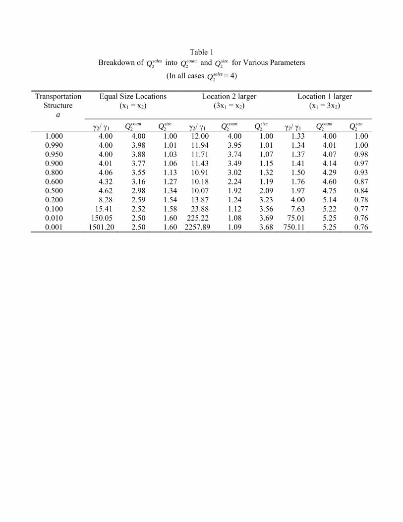
Table 1 Breakdown of salesQ2

into countQ2 and sizeQ2

for Various Parameters

(In all cases salesQ2= 4)

Transportation

Structure a

Equal Size Locations (x1 = x2)

Location 2 larger (3x1 = x2)

Location 1 larger (x1 = 3x2)

γ2/ γ1 countQ2

sizeQ2

γ2/ γ1

countQ2

sizeQ2

γ2/ γ1

countQ2

sizeQ2

1.000 4.00 4.00 1.00 12.00 4.00 1.00 1.33 4.00 1.00 0.990 4.00 3.98 1.01 11.94 3.95 1.01 1.34 4.01 1.00 0.950 4.00 3.88 1.03 11.71 3.74 1.07 1.37 4.07 0.98 0.900 4.01 3.77 1.06 11.43 3.49 1.15 1.41 4.14 0.97 0.800 4.06 3.55 1.13 10.91 3.02 1.32 1.50 4.29 0.93 0.600 4.32 3.16 1.27 10.18 2.24 1.19 1.76 4.60 0.87 0.500 4.62 2.98 1.34 10.07 1.92 2.09 1.97 4.75 0.84 0.200 8.28 2.59 1.54 13.87 1.24 3.23 4.00 5.14 0.78 0.100 15.41 2.52 1.58 23.88 1.12 3.56 7.63 5.22 0.77 0.010 150.05 2.50 1.60 225.22 1.08 3.69 75.01 5.25 0.76 0.001 1501.20 2.50 1.60 2257.89 1.09 3.68 750.11 5.25 0.76

Table 2

A. Nontradeable is retail. Tradeable is manufacturing

Category Number of Plants

Mean Plant Employment

Mean Plant LQ (Industry at Sector Level)

Mean Plant LQ (Industry at 6 digit NAICS Level)

Nontradable 1,118,447 13 1.01 1.09 Tradeable 356,829 46 1.12 2.52

B. Nontradeable includes the bottom ten six-digit NAICS manufacturing industries ranked by average plant employment. Tradeable is rest of manufacturing.

Number of

Plants

Mean Plant Employment

Mean Plant LQ

Export Share

Share of Local

Shipments (less than 50 Miles)

Nontradeable Segment: Individual Industries

Dental laboratories 7,609 6 1.04 .01 .66Retail bakeries 7,119 6 1.27 . .92Quick printing 8,259 6 1.12 .01 .79Fur & leather apparel mfg 224 9 2.17 .06 .34Ice mfg 581 9 1.00 .86Other commercial printing 3,418 10 1.12 .01 .47Tire retreading 750 11 1.17 .00 .Digital printing 386 11 1.17 . .39Canvas & related product mills 1,688 12 1.01 .03 .18Industrial pattern mfg 672 12 2.58 .04 Nontradeable Segment: Mean Over 10 Industries 3,071 7 1.19

.01 .58Tradeable Segment: Mean over remaining 463 Industries 650 51 2.54

.09 .20

C. Classification into Nontradeable and Tradeable is determined through SIC/NAICS cross classification within the given industry Industry Classification Category Number

of Plants

Mean Plant

Employ.

Mean Plant LQ

Export Share

Confectionery mfg from purchased chocolate Nontradeable 440 8

1.42

.00 Tradeable 421 70 2.02 .03 Nonchocolate confectionery mfg Nontradeable 349 4

1.13

.00

Tradeable 276 88 1.88 .03 Bread & bakery product mfg Nontradeable 7,122 6

1.27

.01

Tradeable 3,004 60 1.01 .01 Curtain & drapery mills Nontradeable 1,085 4

1.08

.00

Tradeable 999 21 1.72 .03 Other apparel accessories & other apparel mfg Nontradeable 724 3

1.55

.00 Tradeable 966 25 1.22 .03 Wood kitchen cabinet & counter top mfg Nontradeable 2,055 5

1.17

.00 Tradeable 5,908 15 1.28 .01 Upholstered household furniture mfg Nontradeable 576 5

1.05

.00 Tradeable 1,130 77 9.30 .03 Nonupholstered wood household furniture mfg Nontradeable 815 6

1.61

.00 Tradeable 3,035 41 3.11 .03

D. By Plant Size

Plant Size

Category

Number of Establishment

Mean Plant

Employ.

Mean Plant LQ Export Share Share of Local Shipments (less than 50 Miles)

Raw

NAICS Fixed

Effecte Raw

NAICS Fixed

Effecte Raw

NAICS Fixed

Effecte All 362,829 47 2.52 2.52 .084 .084 .200 .200

1-19 243,081 6 1.60 2.12 .020 .051 .448 .353

20-99 84,826 44 1.92 2.33 ,048 .068 .270 .244100-499 30,140 204 2.56 2.56 .068 .082 .179 .182

500+ 4,782 1,192 3.13 2.71 .115 .095 .177 .192

Source for Panels A through D: Authors calculations based on both the confidential Census micro data as well as public Census data sources.

Table 5

A Comparison of Size Quotients in the Data and in the Two Models High Concentration Industry/Locations

(Locations are Economic Areas) All Economic

Areas Small Areas (less than 1.5 million popopulation)

Large Areas (more than 1.5

million population)

Number of High Concentration Industry/Locations

654 471 183

Mean of salesdataQ 10.11 11.54 6.43

Mean of countdataQ 3.39 3.81 2.30

Mean of sizedataQ 4.64 4.80 4.23

Share of cases where size

elQmod <sizedataQ

Model 1(Tradeables only) .93 .94 .91 Model 2(Tradeables/Nontradeables) .62 .64 .57 Mean of size

datasize

el QQ /mod

Model 1(Tradeables only) .43 .41 .48 Model 2(Tradeables/Nontradeables) .99 .99 1.00

Source: Authors calculations based on estimates of a(.) reported in Table 3 and public Census data on plant locations discussed in the data appendix.

Table 7

Count Quotient in Wood Furniture in High Point, North Carolina Actual Values and Fitted Values for the Two Models

countQ1997

countQ2006 countQ

Actual Data 4.1 2.4 -1.3 Fitted Values Model 1 17.9 20.4 2.5 Model 2 4.0 -3.5 -.5

Table 3

Model Estimates

Transportation Structure (Stage 1)

Stage 2 Results for Estimated Model

Small Plants in Data (employment<=19)

Industry a(100) a(1000) nT nN R2 nN/

(nN+ nT) Count Share

Sales Share

Mean across 82 Industries 0.68 0.29 343.1 1082.5 .33 .70 .62 .10 Ready-mix concrete mfg 0.03 0.00 1548.6 3647.4 0.46 0.70 0.70 0.34Asphalt paving mixture & block mfg 0.11 0.01 307.3 855.7 0.17 0.74 0.86 0.61Concrete block & brick mfg 0.12 0.01 257.1 666.9 0.30 0.72 0.65 0.31Quick printing 0.15 0.02 229.1 7998.9 0.01 0.97 0.95 0.64Mattress mfg 0.15 0.02 235.1 464.9 0.31 0.66 0.60 0.10Truss mfg 0.16 0.02 512.3 467.7 0.59 0.48 0.51 0.12Other concrete product mfg 0.18 0.02 471.1 1822.9 0.21 0.79 0.71 0.17Fluid milk mfg 0.21 0.03 304.8 296.2 0.42 0.49 0.29 0.01Soft drink mfg 0.22 0.03 184.1 422.9 0.26 0.70 0.28 0.01Concrete pipe mfg 0.22 0.03 164.2 246.8 0.44 0.60 0.42 0.13Commercial bakeries 0.28 0.04 81.3 2657.7 0.00 0.97 0.61 0.03Prefabricated wood building mfg 0.33 0.05 319.4 384.6 0.52 0.55 0.65 0.11Other snack food mfg 0.38 0.06 178.4 227.6 0.36 0.56 0.50 0.02Breweries 0.40 0.06 139.8 378.2 0.20 0.73 0.70 0.02Asphalt shingle & coating materials mfg 0.41 0.06 109.4 139.6 0.63 0.56 0.44 0.07Cut stock, resawing lumber, & planing 0.43 0.07 533.0 854.0 0.43 0.62 0.65 0.11Manufactured home (mobile home) mfg 0.43 0.07 283.0 37.0 0.72 0.12 0.10 0.01Custom architectural woodwork & millwork mfg 0.47 0.08 220.1 880.9 0.27 0.80 0.66 0.20Brick & structural clay tile mfg 0.47 0.08 130.9 92.1 0.61 0.41 0.26 0.02Polystyrene foam product mfg 0.48 0.08 144.4 371.6 0.23 0.72 0.45 0.05Commercial lithographic printing 0.50 0.09 3153.1 15373.9 0.20 0.83 0.78 0.15Manifold business form printing 0.50 0.09 214.0 815.0 0.30 0.79 0.45 0.05Wood kitchen cabinet & counter top mfg 0.51 0.09 1590.3 6334.7 0.29 0.80 0.89 0.28Ice cream & frozen dessert mfg 0.54 0.10 79.4 358.6 0.18 0.82 0.66 0.05Specialty canning 0.59 0.13 43.4 93.6 0.33 0.68 0.54 0.01

Other commercial printing 0.60 0.13 449.5 2951.5 0.10 0.87 0.90 0.33Book printing 0.63 0.14 79.9 661.1 0.11 0.89 0.57 0.04Coffee & tea mfg 0.66 0.16 94.2 142.8 0.38 0.60 0.55 0.03Poultry processing 0.69 0.18 282.6 188.4 0.81 0.40 0.18 0.00Wood window & door mfg 0.69 0.18 107.2 1294.8 0.20 0.92 0.66 0.07Blind & shade mfg 0.70 0.19 90.1 392.9 0.11 0.81 0.70 0.08Other millwork (including flooring) 0.70 0.19 215.1 1246.9 0.38 0.85 0.73 0.14Curtain & drapery mills 0.71 0.20 103.7 1964.3 0.05 0.95 0.91 0.24Flour mixes & dough mfg from purchased flour 0.72 0.20 92.1 156.9 0.47 0.63 0.52 0.04Commercial screen printing 0.72 0.20 1210.4 2905.6 0.53 0.71 0.81 0.21Upholstered household furniture mfg 0.73 0.21 858.4 845.6 0.90 0.50 0.69 0.05Sign mfg 0.73 0.21 930.7 4743.3 0.26 0.84 0.84 0.22Sanitary paper product mfg 0.73 0.21 61.1 74.9 0.53 0.55 0.35 0.01Marking device mfg 0.73 0.21 89.7 540.3 0.22 0.86 0.88 0.29Fruit & vegetable canning 0.75 0.23 304.4 499.6 0.60 0.62 0.49 0.03Institutional furniture mfg 0.76 0.24 233.2 774.8 0.39 0.77 0.63 0.09Nonupholstered wood household furniture mfg 0.78 0.26 673.7 3161.3 0.38 0.82 0.81 0.08Showcase, partition, shelving, & locker mfg 0.79 0.27 932.7 1214.3 0.37 0.57 0.62 0.10Confectionery mfg from purchased chocolate 0.81 0.30 136.7 706.3 0.10 0.84 0.77 0.04Metal tank (heavy gauge) mfg 0.82 0.31 328.3 279.7 0.63 0.46 0.36 0.04All other leather good mfg 0.83 0.32 132.2 348.8 0.18 0.73 0.80 0.13Pharmaceutical preparation mfg 0.83 0.32 371.9 460.1 0.48 0.55 0.48 0.01Vitreous china, fine earthenware, & other potter 0.83 0.32 214.8 826.2 0.13 0.79 0.80 0.11Metal household furniture mfg 0.83 0.34 126.5 293.5 0.35 0.70 0.66 0.06Fastener, button, needle, & pin mfg 0.83 0.34 14.8 236.2 0.05 0.94 0.71 0.10Mayonnaise, dressing, & other prepared sauce mfg 0.85 0.36 37.3 285.7 0.09 0.88 0.65 0.04Broom, brush, & mop mfg 0.85 0.36 89.4 241.6 0.31 0.73 0.55 0.07Frozen specialty food mfg 0.86 0.38 68.4 341.6 0.23 0.83 0.48 0.02Other metalworking machinery mfg 0.86 0.39 286.7 185.3 0.58 0.39 0.53 0.07Other household textile product mills 0.86 0.39 247.6 512.4 0.52 0.67 0.53 0.03Nonchocolate confectionery mfg 0.87 0.41 126.3 491.7 0.20 0.80 0.77 0.03Industrial mold mfg 0.87 0.41 2123.6 396.4 0.84 0.16 0.72 0.23Toilet preparation mfg 0.88 0.42 273.6 445.4 0.34 0.62 0.57 0.02Other commercial & service industry machinery mf 0.88 0.42 436.3 915.7 0.38 0.68 0.63 0.08All other miscellaneous food mfg 0.88 0.43 151.0 688.0 0.23 0.82 0.62 0.06Men's & boys' cut & sew suit, coat, & overcoat m 0.88 0.43 62.0 159.0 0.25 0.72 0.43 0.04

Hat, cap, & millinery mfg 0.88 0.43 48.7 339.3 0.14 0.87 0.59 0.08Power-driven handtool mfg 0.89 0.44 23.6 193.4 0.08 0.89 0.70 0.05Women's & girls' cut & sew suit, coat, skirt mfg 0.89 0.44 154.9 282.1 0.24 0.65 0.53 0.12Other apparel accessories & other apparel mfg 0.89 0.44 756.7 906.3 0.57 0.54 0.84 0.17Electronic computer mfg 0.91 0.51 87.5 469.5 0.26 0.84 0.63 0.01Boat building 0.91 0.51 458.0 564.0 0.37 0.55 0.71 0.08Heating equipment (except warm air furnaces) mfg 0.92 0.53 134.6 332.4 0.18 0.71 0.61 0.06Sporting & athletic goods mfg 0.92 0.54 879.6 1664.4 0.50 0.65 0.78 0.10Ophthalmic goods mfg 0.92 0.54 95.7 473.3 0.19 0.83 0.72 0.06Blankbook, looseleaf binder, & device mfg 0.92 0.54 108.9 190.1 0.43 0.64 0.45 0.04Surgical & medical instrument mfg 0.93 0.57 485.3 1108.7 0.35 0.70 0.63 0.04Other lighting equipment mfg 0.93 0.58 39.2 291.8 0.11 0.88 0.54 0.05Game, toy, & children's vehicle mfg 0.94 0.59 68.4 709.6 0.11 0.91 0.74 0.07Pen & mechanical pencil mfg 0.94 0.59 27.7 82.3 0.23 0.75 0.55 0.03Audio & video equipment mfg 0.94 0.59 139.1 411.9 0.22 0.75 0.64 0.04Surgical appliance & supplies mfg 0.95 0.65 197.1 1444.9 0.15 0.88 0.64 0.05Women's & girls' cut/sew lingerie & nightwear mf 0.95 0.66 75.6 207.4 0.34 0.73 0.44 0.05Telephone apparatus mfg 0.96 0.73 245.3 350.7 0.68 0.59 0.44 0.01Other communications equipment mfg 0.97 0.78 128.3 364.7 0.28 0.74 0.68 0.05Musical instrument mfg 0.98 0.82 136.2 431.8 0.34 0.76 0.82 0.12Women's & girls' cut & sew other outerwear mfg 0.98 0.82 381.4 482.6 0.42 0.56 0.54 0.05

Source: Authors calculations based on estimates of a(.) reported in Table 3 and public Census data on plant locations discussed in the data appendix.

Table 4

BEA Economic Area Industry Data Models Models relative to Data

salesdataQ

countdataQ

sizedataQ

sizeQ1 sizeQ2

sizedata

size QQ /1 sizedata

size QQ /2

Greensboro--Winston-Salem--High Point, NC

Nonupholstered wood house-hold furniture mfg

27.1 4.1 6.6 1.5 6.8 0.2 1.0

Charlotte-Gastonia-Salisbury, NC-SC Upholstered household furniture mfg

22.3 10.9 2.1 1.4 2.6 0.7 1.3

Nashville-Davidson--Murfreesboro--Columbia, TN

Pen & mechanical pencil mfg 21.4 3.1 6.9 1.2 4.1 0.2 0.6

Buffalo-Niagara-Cattaraugus, NY Hat, cap, & millinery mfg 19.1 1.4 13.3 1.1 6.4 0.1 0.5Hartford-West Hartford-Willimantic,

CT Game, toy, & children's

vehicle mfg 19.0 2.8 6.8 1.1 7.6 0.2 1.1

Harrisburg-Carlisle-Lebanon, PA Specialty canning 18.7 2.0 9.2 1.6 4.2 0.2 0.5Denver-Aurora-Boulder, CO Breweries 14.5 4.5 3.3 1.8 4.9 0.5 1.5Rochester-Batavia-Seneca Falls, NY Ophthalmic goods mfg 14.4 3.2 4.4 1.2 4.9 0.3 1.1Memphis, TN-MS-AR Power-driven handtool mfg 14.3 1.3 10.7 1.2 6.5 0.1 0.6Sacramento--Arden-Arcade--

Truckee, CA-NV Electronic computer mfg 13.3 2.1 6.2 0.9 4.3 0.2 0.7

Birmingham-Hoover-Cullman, AL Manufactured home (mobile home) mfg

12.8 9.1 1.4 1.6 1.8 1.1 1.3

Jackson-Yazoo City, MS Poultry processing 12.5 7.5 1.7 1.1 1.8 0.7 1.1Grand Rapids-Muskegon-Holland,

MI Nonchocolate confectionery

mfg 11.3 1.2 9.2 1.3 4.3 0.1 0.5

Salt Lake City-Ogden-Clearfield, UT Asphalt paving mixture & block mfg

11.0 0.7 16.1 2.6 6.0 0.2 0.4

San Antonio, TX Curtain & drapery mills 10.3 0.6 16.8 0.8 6.5 0.0 0.4Virginia Beach-Norfolk-Newport

News, VA-NC Coffee & tea mfg 10.3 2.0 5.1 1.2 2.6 0.2 0.5

Indianapolis-Anderson-Columbus, IN Audio & video equipment mfg 10.0 1.4 6.9 1.2 3.6 0.2 0.5

Source: Authors calculations based on estimates of a(.) reported in Table 3 and public Census data on plant locations discussed in the data appendix. Model 1 is tradables only. Model 2 includes tradables and nontradables.

Table 6 Geographic Concentration of Textile, Clothing, and Furniture Industries

Mean

Plant LQ

%Δ plant count

%Δ plant

employ

Import share of all shipments

China Share of Imports

Slope of count

elQmod

R2

Industry 1997 2006 1997 2007 Mod1 Mod2 Mod1 Mod2

High Geographic Concentration

Upholstered household furniture mfg 8.7 -10.7 -9.7 7.8 21.7 5.5 65.2 -0.88 1.58 0.49 0.37 Other household textile product mills 3.3 -17.4 -44.8 22.1 61.2 25.4 48.9 -0.16 0.58 0.00 0.02 Nonupholstered wood household furniture mfg 3.2 -4.5 -41.4 29.5 55.9 18.5 46.2 -0.62 1.69 0.17 0.14 Hat, cap, & millinery mfg 2.6 -51.3 -69.8 44.2 72.3 26.3 66.5 -1.06 0.38 0.02 0.00 Men's & boys' cut & sew suit, coat, & overcoat m 2.2 -12.7 -63.9 40.6 69.1 6.5 28.6 -0.38 2.26 0.00 0.09 Women's & girls' cut/sew lingerie & nightwear mf 2.1 -63.7 -85.4 44.5 80.0 10.8 37.2 -7.06 1.92 0.26 0.11 Women's & girls' cut & sew suit, coat, skirt mfg 2.1 -70.3 -87.9 47.5 90.7 18.6 48.7 -1.63 0.82 0.09 0.03 Curtain & drapery mills 1.6 -23.6 -51.1 8.5 49.7 37.8 65.3 0.01 0.79 0.00 0.00 Metal household furniture mfg 1.5 -15.9 -42.4 28.8 56.6 36.8 85.4 -1.07 1.44 0.02 0.07 Women's & girls' cut & sew other outerwear mfg 1.5 -37.6 -73.9 55.7 87.5 16.4 34.0 -14.08 0.15 0.21 0.00 Institutional furniture mfg 1.4 -34.0 -27.4 54.4 76.2 18.1 52.9 0.53 -0.04 0.02 0.00 Other apparel accessories & other apparel mfg 1.3 -62.6 -66.3 39.0 76.6 34.8 63.7 -0.12 0.92 0.00 0.04 Low Geographic Concentration Wood kitchen cabinet & counter top mfg 1.25 20.7 50.1 3.2 4.2 2.0 34.8 -0.37 -0.89 0.03 0.06 Showcase, partition, shelving, & locker fg 1.2 -19.5 -20.0 14.4 33.3 11.5 49.2 0.29 -0.50 0.01 0.02 Blind & shade mfg 1.1 1.0 9.8 13.8 27.2 54.9 63.1 0.18 0.61 0.00 0.01 Custom architectural woodwork & millwork mfg 1.1 42.4 44.2 . . . . 0.31 1.76 0.01 0.10 Mattress mfg 1.0 -20.1 6.0 0.7 3.4 2.4 47.4 0.20 0.27 0.01 0.00

Mean High Geographic Concentration 2.6 -33.7 -55.3 35.2 66.4 21.3 53.5 -2.21 1.04 0.11 .07 Mean Low Geographic Concentration 1.1 4.9 18.0 8.0 17.0 17.7 48.6 0.12 0.25 0.01 .04

Figure 1

Sm

all P

lant

Sha

re

0.0

0.1

0.2

0.3

0.4

0.5

0.6

0.7

0.8

0.9

1.0

Nontradeable Plant Share

0.0 0.1 0.2 0.3 0.4 0.5 0.6 0.7 0.8 0.9 1.0