DEPARTMENT OF ECONOMICS UNIVERSITY OF CYPRUS

AN ALTERNATIVE ASYMPTOTIC ANALYSIS OF RESIDUAL-BASED STATISTICS

Elena Andreou and Bas J.M. Werker

Discussion Paper 2010-08

P.O. Box 20537, 1678 Nicosia, CYPRUS Tel.: ++357-22893700, Fax: ++357-22895028

Web site: http://www.econ.ucy.ac.cy

An Alternative Asymptotic Analysis of

Residual-Based Statistics

Elena Andreou∗ and Bas J.M. Werker†

University of Cyprus and Tilburg University

This version: June 2010

∗Department of Economics, University of Cyprus, P.O.Box 537, CY1678, Nicosia,

Cyprus. Tel +357 22 892449, fax +357 22 892432, e-mail Elena.Andreou@ucy.ac.cy.†Corresponding author: Econometrics and Finance Group, CentER, Tilburg University,

P.O.Box 90153, 5000 LE, Tilburg, The Netherlands. Tel +31 13 4662532, fax +31 13

4662875, e-mail Werker@TilburgUniversity.nl.

1

Abstract

This paper presents an alternative method to derive the limiting

distribution of residual-based statistics. Our method does not impose

an explicit assumption of (asymptotic) smoothness of the statistic of

interest with respect to the model’s parameters. and, thus, is especially

useful in cases where such smoothness is difficult to establish. Instead,

we use a locally uniform convergence in distribution condition, which

is automatically satisfied by residual-based specification test statistics.

To illustrate, we derive the limiting distribution of a new functional

form specification test for discrete choice models, as well as a runs-

based tests for conditional symmetry in dynamic volatility models.

JEL codes: C32, C51, C52.

Keywords: Le Cam’s third lemma, Local Asymptotic Normality (LAN).

2

1 Introduction

Residual-based tests are generally used for diagnostic checking of a proposed

statistical model. Such specification tests are covered in many textbooks and

remain of interest in ongoing research. Similarly, residual-based estimators

(often referred to as two-step estimators) are widely applied in econometric

work. Traditionally, the asymptotic distribution of residual-based statistics

(be it tests or estimators) is derived using a particular model specification,

some more or less stringent assumptions about the statistic, and conditions

on the first-step estimator employed. A key assumption is some form of

(asymptotic) smoothness of the statistic with respect to the parameter to

be estimated as formalized first in Pierce (1982) and Randles (1982). Since

then, this approach has been significantly extended in, e.g., Pollard (1989),

Newey and McFadden (1994), and Andrews (1994).

We present a new and alternative approach that does not involve explicit

smoothness conditions for the statistic of interest. Instead, we rely on a lo-

cally uniform weak convergence assumption which is shown to be generally

(automatically) satisfied by residual-based statistics. Our approach offers a

useful and unifying alternative, especially when smoothness conditions are

nontrivial to establish or require additional regularity. Some examples of such

3

statistics are, for instance, rank-based statistics (see, e.g., Hallin and Puri,

1991) and statistics based on non-differentiable forecast error loss functions

(e.g. McCracker, 2000). Abadie and Imbens (2009) present an application of

our method to derive the asymptotic distribution theory of matching esti-

mators based on the estimated propensity score that can be a non-smooth

function of the estimated parameters and for which standard bootstrap in-

ference is often not valid (Abadie and Imbens, 2008). In applications where

the statistic of interest is smooth, our conditions can be checked along the

traditional lines. In order to illustrate our approach, we derive the limit-

ing distribution of a new test based on Kendall’s tau for omitted variables

in binary choice models and a runs-based test for conditional symmetry in

dynamic volatility models.

Our proposed method applies to general model specifications, as long as

they satisfy the Uniform Local Asymptotic Normality (ULAN) condition.

Most of the standard econometric models satisfy this condition; see Sec-

tion 3.1 below for a more detailed discussion. The ULAN condition is central

in the Hajek and Le Cam’s theory of asymptotic statistics (see, e.g., Bickel

et al., 1993, Le Cam and Yang, 1990, Pollard, 2004, and van der Vaart,

1998). We use this theory to derive our results. Other advances in economet-

4

ric theory using the LAN approach can be found in, e.g., Abadir and Distaso

(2007), Jeganathan (1995), and Ploberger (2004). For ULAN models, our re-

sults offer a simple, yet general, method to derive the asymptotic distribution

of residual-based statistics using initial√n-consistent estimators. Under the

conditions imposed, our main Theorem 3.1 asserts that the residual-based

statistic is asymptotically normally distributed with a variance that is a sim-

ple function of the limiting variances/covariances of the innovation-based

statistic1, the central sequence (the ULAN equivalent of the derivative of the

log-likelihood), and the estimator. Using this approach, we can readily obtain

the local power of such residual-based tests, which can also be interpreted

in terms of specification tests with locally misspecified alternatives such as

in Bera and Yoon (1993). In particular, this allows one to assess in which

situations the local power of the residual-based test exceeds, falls below, or

equals that of the innovation-based test.

To illustrate our method, we consider two applications. First, we derive

the asymptotic distribution of a new nonparametric test for omitted variables

in a binary choice model. Second, we discuss a runs-based test for conditional

1Throughout the paper, we use the term innovation-based statistic for the statistic

applied to the true innovations in the model, i.e., the statistic obtained if the true value

of the model parameters were used.

5

symmetry in dynamic volatility models. These applications purposely focus

on non-parametric statistics as these are usually defined in terms of inherently

non-smooth statistics like ranks, signs, runs, etc. For these applications, an

appropriate form of asymptotic smoothness can probably be established, but

our technique offers a useful alternative for which this is not necessary. Our

applications are introduced in Section 2. A number of additional applications

of our method can be found in Andreou and Werker (2009).

Although the present paper mainly deals with residual-based testing, the

results can directly be applied in the area of two-step estimation when as-

sessing the estimation error in a second-step estimator calculated from the

residuals of a model estimated in a first step. This problem has received large

attention in the econometrics literature, see, e.g, Murphy and Topel (1985,

2002) and Pagan (1986). In the notation below, this would merely mean that

the statistic Tn should be taken as the second-step estimation error.

The rest of this paper is organized as follows. The next section introduces

the applications we use to illustrate the scope of our technique. Section 3.1

then presents the conditions we need to derive the limiting distribution of

a residual-based statistic. Our main result is stated and discussed in Sec-

tion 3.2. Section 3.3 uses our main theorem to derive the (local) power of

6

residual-based tests and compares this with the local power of the under-

lying innovation-based tests. We indicate that a technical issue arises when

making our ideas rigorous. Section 4 addresses this by discretization and

we provide a formal proof of our main result. Section 5 concludes and the

appendix contains the proofs and some auxiliary results.

2 Two motivational applications

2.1 Omitted variable test for the Binary Choice model

Consider the binary choice model

IP{Y = 1|X} = F (XT θ), (2.1)

where Y denotes a binary response variable, X some exogenous explanatory

variables, and F a given probability distribution function. We assume that

the distribution function F admits a continuous density f and that the Fisher

Information matrix

IF (θ) = Ef(XT θ)2

F (XT θ) (1− F (XT θ))XXT , (2.2)

exists and is continuous in θ. For inference, an i.i.d. sample of observations

(Yi, Xi), i = 1, . . . , n, is available.

7

The generalized residuals, for given parameter value θ, are defined as

εGi (θ) =Yi − F (XT

i θ)

F (XTi θ) (1− F (XT

i θ))f(XT

i θ) (2.3)

The classical test for functional specification checks for a possibly omitted

variable Zi using the statistic

Tn(θ) =1√n

n∑i=1

εGi (θ)Zi. (2.4)

The statistic Tn(θ) is innovation based as it depends on the unknown true

value of the parameter θ. The limiting distribution of this innovation-based

statistic follows immediately from the classical Central Limit Theorem as

soon as εGi (θ)Zi has finite variance and zero mean.

In applications, the unknown parameter θ is replaced by an estimator

θn, for instance, the maximum likelihood estimator θ(ML)n . This leads to the

residual-based statistic Tn(θn). The traditional way of deriving the limiting

distribution of Tn(θn) relies on linearizing the statistic Tn(θ); see, for instance,

Pagan and Vella (1989). This approach leads to

Tn(θn)L−→ N

(0,EWZZT − EWXZT

(EWXXT

)−1 EWXZT), (2.5)

as n→∞, with

W =f(XT θ)2

F (XT θ) (1− F (XT θ)).

8

The test statistic (2.4) checks for linear correlation between the general-

ized residuals and the possibly omitted variable Z. One could also be inter-

ested in a test with power against nonlinear forms of dependence based on

Kendall’s tau applied to the pairs (εGi (θ), Zi). For simplicity we consider the

case where the possibly omitted variables are univariate, i.e., Zi ∈ IR. Recall

that the population version of Kendall’s tau is defined as

τ = 4IP{εGi (θ) < εGj (θ), Zi < Zj} − 1, i 6= j. (2.6)

An appropriately scaled innovation-based version of Kendall’s tau is the U -

statistic

T τn (θ) =√n

n

2

−1

n∑i=1

i−1∑j=1

[4I{εGi (θ) < εGj (θ), Zi < Zj} − 1

]L−→ N

(0,

4

9

).

This limiting distribution, under the null hypothesis of independent εGi and

Zi, can be obtained using the projection theorem for U -statistics, e.g., The-

orem 12.3 in van der Vaart (1998).

Deriving the limiting distribution of the residual-based statistic T τn (θn)

using linearizion is less obvious due to the inherent non-differentiability of the

indicator functions in T τn (θ). Our approach to residual-based statistics will

9

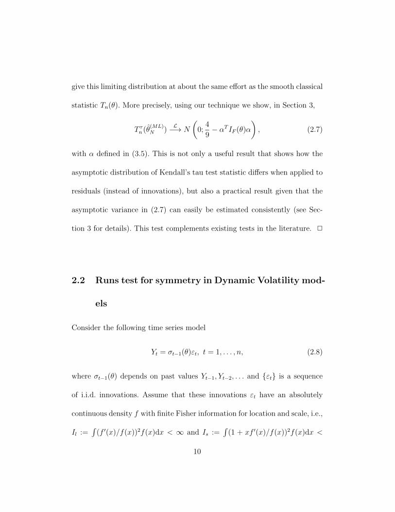
give this limiting distribution at about the same effort as the smooth classical

statistic Tn(θ). More precisely, using our technique we show, in Section 3,

T τn (θ(ML)N )

L−→ N

(0;

4

9− αT IF (θ)α

), (2.7)

with α defined in (3.5). This is not only a useful result that shows how the

asymptotic distribution of Kendall’s tau test statistic differs when applied to

residuals (instead of innovations), but also a practical result given that the

asymptotic variance in (2.7) can easily be estimated consistently (see Sec-

tion 3 for details). This test complements existing tests in the literature. 2

2.2 Runs test for symmetry in Dynamic Volatility mod-

els

Consider the following time series model

Yt = σt−1(θ)εt, t = 1, . . . , n, (2.8)

where σt−1(θ) depends on past values Yt−1, Yt−2, . . . and {εt} is a sequence

of i.i.d. innovations. Assume that these innovations εt have an absolutely

continuous density f with finite Fisher information for location and scale, i.e.,

Il :=∫

(f ′(x)/f(x))2f(x)dx < ∞ and Is :=∫

(1 + xf ′(x)/f(x))2f(x)dx <

10

∞. Finally, impose Eεt = 0, Eε2t = 1, and κε := Eε4t < ∞ and assume

that a stationary and ergodic solution to (2.8) exists. These are standard

assumptions for most GARCH-type models.

Many specification tests concerning the innovations in stochastic volatility

models have been introduced and studied in the literature. We consider a

nonparametric test of conditional symmetry based on Wald-Wolfowitz runs.

One advantage of such a test is that it does not require the existence of

any higher order moments of the innovation distribution and, thus, can be

considered robust to different distributions and outliers. This is particularly

relevant given that there is no consensus in the empirical literature as to the

form of heavy-tailed distributions in, e.g., financial time series. This test for

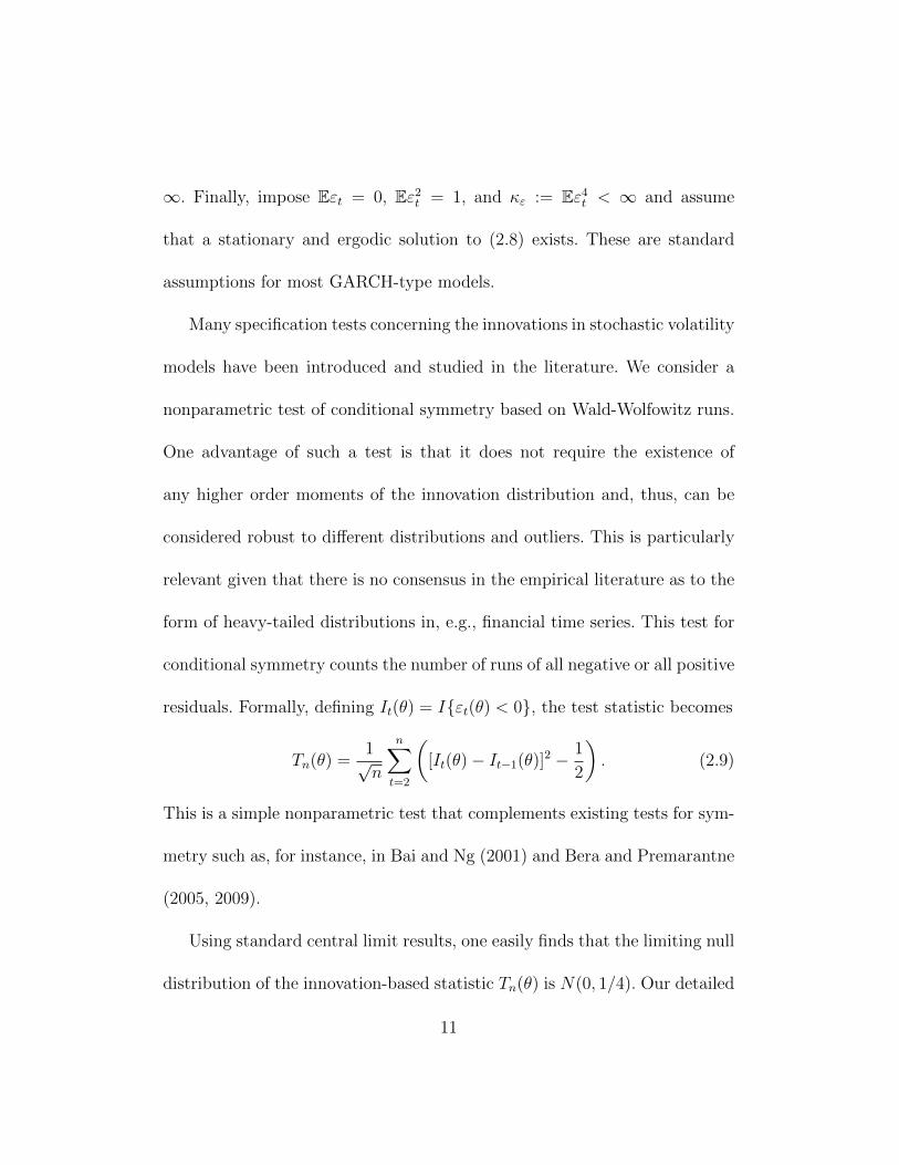
conditional symmetry counts the number of runs of all negative or all positive

residuals. Formally, defining It(θ) = I{εt(θ) < 0}, the test statistic becomes

Tn(θ) =1√n

n∑t=2

([It(θ)− It−1(θ)]2 −

1

2

). (2.9)

This is a simple nonparametric test that complements existing tests for sym-

metry such as, for instance, in Bai and Ng (2001) and Bera and Premarantne

(2005, 2009).

Using standard central limit results, one easily finds that the limiting null

distribution of the innovation-based statistic Tn(θ) is N(0, 1/4). Our detailed

11

results in Section 3 show that this asymptotic null distribution needs not be

adapted when applied to residuals of dynamic volatility models. The results

in Section 3.3 furthermore show that the asymptotic local power of this runs

test is the same whether applied to innovations or to residuals. 2

3 Main results

Our results are derived using the Hajek and Le Cam techniques of asymptotic

statistics. We first introduce the assumptions needed. Subsequently, we will

derive the asymptotic size and local power of residual-based tests.

3.1 Assumptions

Let us formally introduce the models we consider in this paper. Thereto, let

E (n) denote a sequence of experiments defined on a common parameter set

Θ ⊂ IRk:

E (n) ={X(n),A(n),P(n) =

(IP

(n)θ : θ ∈ Θ

)},

where(X(n),A(n)

)is a sequence of measurable spaces and, for each n and θ ∈

Θ, IP(n)θ a probability measure on

(X(n),A(n)

). We assume throughout this

12

paper that Θ is a subset of IRk so that we consider the effect of pre-estimating

a Euclidean parameter. We also assume that pertinent asymptotics in the

sequence of experiments take place at the usual√n rate. Other rates, as

occur, for instance, in non-stationary time series, can be easily adopted at

the cost of more cumbersome notation only.

Our analysis is based on two assumptions. The first is Condition (ULAN)

that imposes regularity on the model at hand. This condition involves nei-

ther the statistic Tn nor the estimator θn. During the last thirty years, the

ULAN condition has been established for most standard cross-section and

time-series models. To introduce the condition, let θ0 ∈ Θ denote a fixed

value of the Euclidean parameter and let (θn) and (θ′n) denote sequences

contiguous to θ0, i.e., δn =√n(θn − θ0) and δ′n =

√n(θ′n − θ0) are bounded

in IRk. Write Λ(n)(θ′n|θn) = log(

dIP(n)θ′n/dIP

(n)θn

)for the log-likelihood of IP

(n)θ′n

with respect to IP(n)θn

. In case IP(n)θ′n

is not dominated by IP(n)θn

, we mean the

Radon-Nikodym derivative of the absolute continuous part in the Lebesgue

decomposition of IP(n)θ′n

with respect to IP(n)θn

(see Strasser, 1985, Definition 1.3).

Condition (ULAN): The sequence of experiments E (n) is Uniformly Locally

Asymptotically Normal (ULAN) in the sense that there exists a sequence of

13

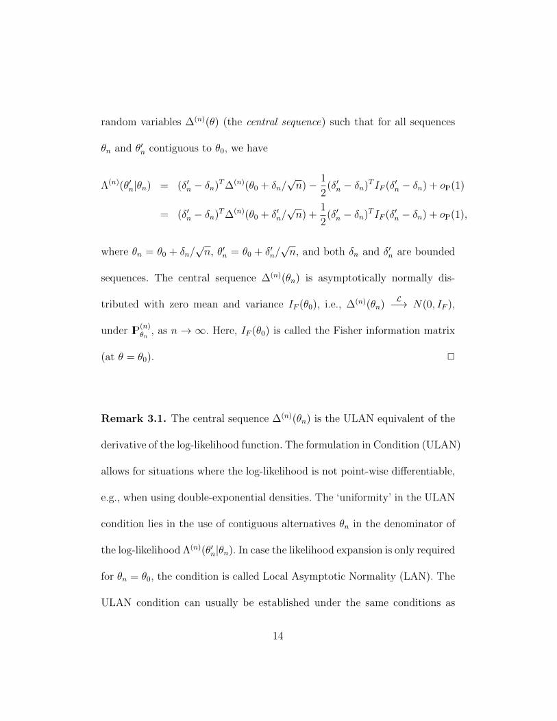
random variables ∆(n)(θ) (the central sequence) such that for all sequences

θn and θ′n contiguous to θ0, we have

Λ(n)(θ′n|θn) = (δ′n − δn)T∆(n)(θ0 + δn/√n)− 1

2(δ′n − δn)T IF (δ′n − δn) + oIP(1)

= (δ′n − δn)T∆(n)(θ0 + δ′n/√n) +

1

2(δ′n − δn)T IF (δ′n − δn) + oIP(1),

where θn = θ0 + δn/√n, θ′n = θ0 + δ′n/

√n, and both δn and δ′n are bounded

sequences. The central sequence ∆(n)(θn) is asymptotically normally dis-

tributed with zero mean and variance IF (θ0), i.e., ∆(n)(θn)L−→ N(0, IF ),

under IP(n)θn

, as n → ∞. Here, IF (θ0) is called the Fisher information matrix

(at θ = θ0). 2

Remark 3.1. The central sequence ∆(n)(θn) is the ULAN equivalent of the

derivative of the log-likelihood function. The formulation in Condition (ULAN)

allows for situations where the log-likelihood is not point-wise differentiable,

e.g., when using double-exponential densities. The ‘uniformity’ in the ULAN

condition lies in the use of contiguous alternatives θn in the denominator of

the log-likelihood Λ(n)(θ′n|θn). In case the likelihood expansion is only required

for θn = θ0, the condition is called Local Asymptotic Normality (LAN). The

ULAN condition can usually be established under the same conditions as

14

LAN. We need the uniform version in the proof of our main result essentially

due to the fact that residual-based statistics are calculated using residuals

based on (random) local alternatives θn. Note that the ULAN condition as

such is simply an assumption relating to the model and does not affect the

(non)smoothness assumption of the statistic one wishes to consider. 2

Remark 3.2. The ULAN condition presents a prime example in the the-

ory of convergence of statistical experiments. The quadratic expansion of

the log-likelihood ratio in the local parameter δ′n − δn is equal to the log-

likelihood ratio in the Gaussian shift model {N(IF (θ0)−1δ, IF (θ0)

−1) : δ ∈

IRk}. This can be shown to imply that the sequence of localized experiments

{IP(n)θn+δ

: δ ∈ IRk} converges, in an appropriate sense, to the Gaussian shift

experiment. This in turn implies that asymptotic analysis in the original ex-

periments can be based on properties of the limiting Gaussian shift model.

A useful consequence of the ULAN, or even LAN, property is that the se-

quences IP(n)θ′n

and IP(n)θ′n

are contiguous (see, e.g., Le Cam and Yang, 1990,

or van der Vaart, 1998). As a result, convergence in probability under IP(n)θn

is equivalent to convergence under IP(n)θ′n

. In particular, any oIP(1)-terms in

Condition (ULAN), and in the remainder of this paper, hold simultaneously

under IP(n)θ0

, IP(n)θn

, and IP(n)θ′n

. 2

15

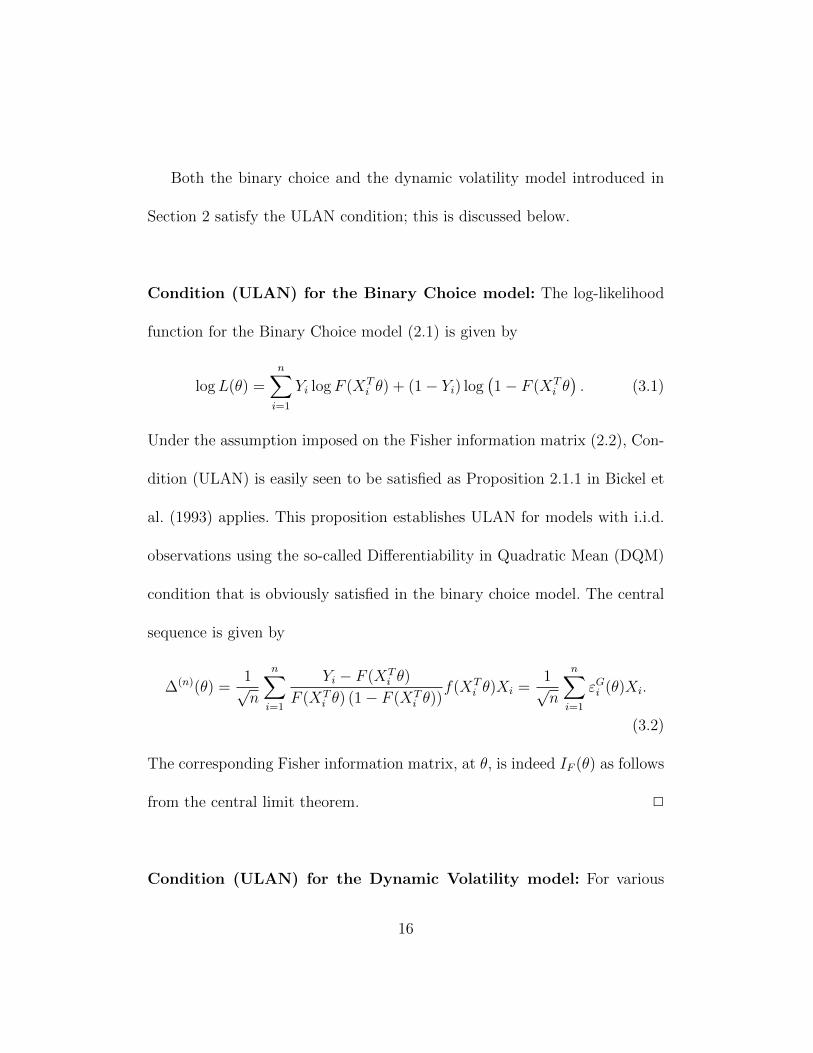
Both the binary choice and the dynamic volatility model introduced in

Section 2 satisfy the ULAN condition; this is discussed below.

Condition (ULAN) for the Binary Choice model: The log-likelihood

function for the Binary Choice model (2.1) is given by

logL(θ) =n∑i=1

Yi logF (XTi θ) + (1− Yi) log

(1− F (XT

i θ). (3.1)

Under the assumption imposed on the Fisher information matrix (2.2), Con-

dition (ULAN) is easily seen to be satisfied as Proposition 2.1.1 in Bickel et

al. (1993) applies. This proposition establishes ULAN for models with i.i.d.

observations using the so-called Differentiability in Quadratic Mean (DQM)

condition that is obviously satisfied in the binary choice model. The central

sequence is given by

∆(n)(θ) =1√n

n∑i=1

Yi − F (XTi θ)

F (XTi θ) (1− F (XT

i θ))f(XT

i θ)Xi =1√n

n∑i=1

εGi (θ)Xi.

(3.2)

The corresponding Fisher information matrix, at θ, is indeed IF (θ) as follows

from the central limit theorem. 2

Condition (ULAN) for the Dynamic Volatility model: For various

16

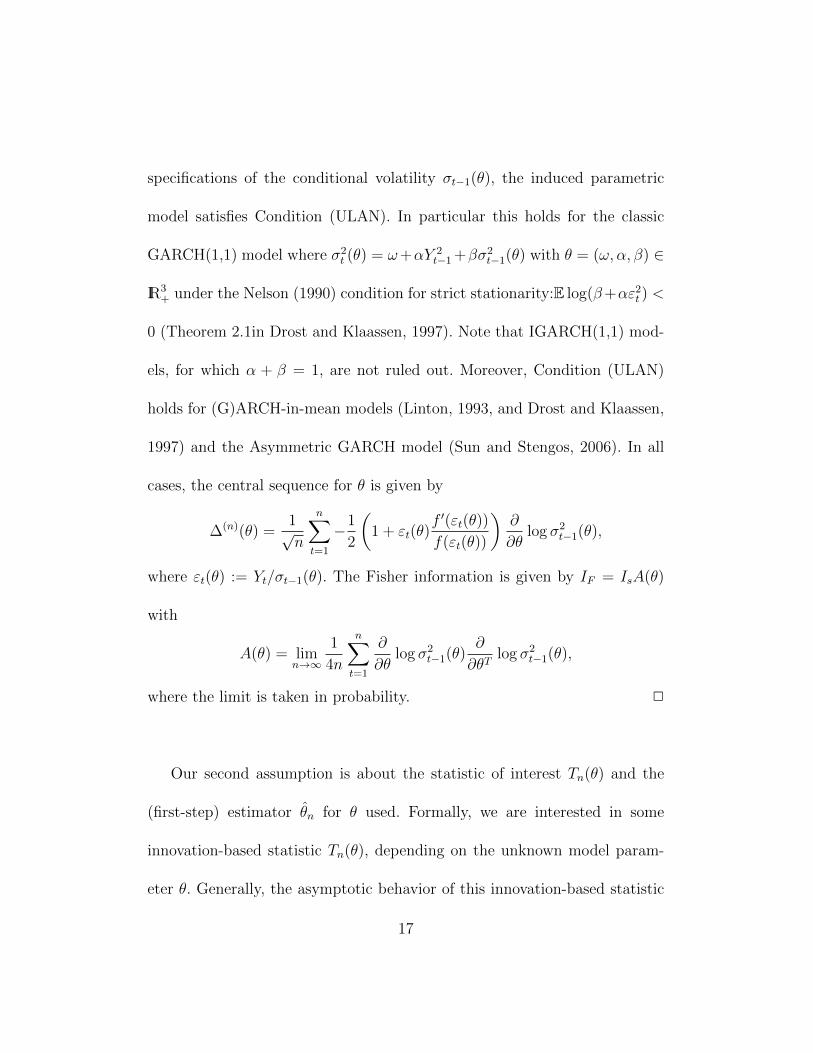
specifications of the conditional volatility σt−1(θ), the induced parametric

model satisfies Condition (ULAN). In particular this holds for the classic

GARCH(1,1) model where σ2t (θ) = ω+αY 2

t−1 +βσ2t−1(θ) with θ = (ω, α, β) ∈

IR3+ under the Nelson (1990) condition for strict stationarity:E log(β+αε2t ) <

0 (Theorem 2.1in Drost and Klaassen, 1997). Note that IGARCH(1,1) mod-

els, for which α + β = 1, are not ruled out. Moreover, Condition (ULAN)

holds for (G)ARCH-in-mean models (Linton, 1993, and Drost and Klaassen,

1997) and the Asymmetric GARCH model (Sun and Stengos, 2006). In all

cases, the central sequence for θ is given by

∆(n)(θ) =1√n

n∑t=1

−1

2

(1 + εt(θ)

f ′(εt(θ))

f(εt(θ))

)∂

∂θlog σ2

t−1(θ),

where εt(θ) := Yt/σt−1(θ). The Fisher information is given by IF = IsA(θ)

with

A(θ) = limn→∞

1

4n

n∑t=1

∂

∂θlog σ2

t−1(θ)∂

∂θTlog σ2

t−1(θ),

where the limit is taken in probability. 2

Our second assumption is about the statistic of interest Tn(θ) and the

(first-step) estimator θn for θ used. Formally, we are interested in some

innovation-based statistic Tn(θ), depending on the unknown model param-

eter θ. Generally, the asymptotic behavior of this innovation-based statistic

17

follows easily from classical limit arguments. The focus of interest of the

present paper is the asymptotic behavior of the residual-based statistic Tn(θ)

obtained by replacing the true value of θ by some estimate θn.

Traditionally, following Pierce (1982) and Randles (1982), several papers

analyze the asymptotic behavior of the residual-based statistic relying on a

condition like

Tn(θ0 + δn/√n) = Tn(θ0)− cT δn + oIP(1), (3.3)

under IP(n)θ0

, for bounded sequences δn. Condition (3.3) is sometimes rein-

forced to hold for random sequences δn = OIP(1). However, this reinforce-

ment is generally not required if one would resort to discretized estimators

as in Section 4. In the ubiquitous case that the statistic Tn(θ) is, up to

op(1)-terms, some average n−1/2∑n

t=1m(Xt; θ) of expectation-zero functions

m of observations X1, . . . , Xn, Condition (3.3) is verified if m is differen-

tiable in θ (a route, for instance, followed in Newey and McFadden, 1994) or

if Em(Xt; θ) is differentiable in θ as in, e.g., the empirical process approach

of Andrews (1994).

Given (3.3), the limiting distribution of Tn(θn) is subsequently obtained,

18

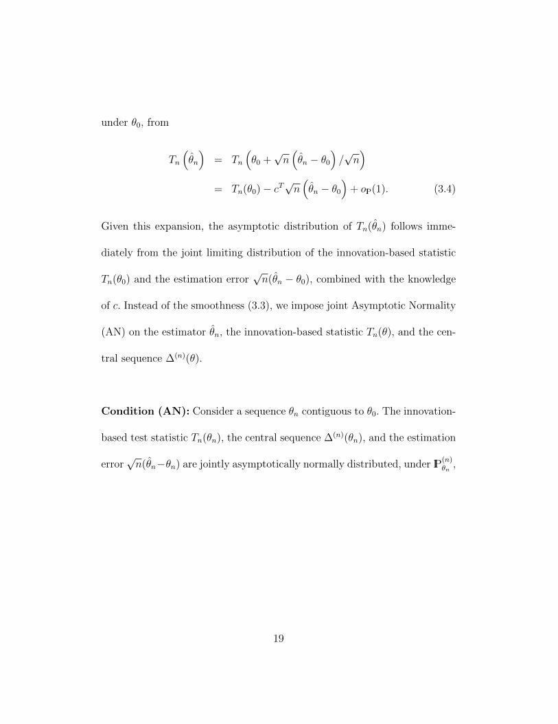
under θ0, from

Tn

(θn

)= Tn

(θ0 +

√n(θn − θ0

)/√n)

= Tn(θ0)− cT√n(θn − θ0

)+ oIP(1). (3.4)

Given this expansion, the asymptotic distribution of Tn(θn) follows imme-

diately from the joint limiting distribution of the innovation-based statistic

Tn(θ0) and the estimation error√n(θn − θ0), combined with the knowledge

of c. Instead of the smoothness (3.3), we impose joint Asymptotic Normality

(AN) on the estimator θn, the innovation-based statistic Tn(θ), and the cen-

tral sequence ∆(n)(θ).

Condition (AN): Consider a sequence θn contiguous to θ0. The innovation-

based test statistic Tn(θn), the central sequence ∆(n)(θn), and the estimation

error√n(θn−θn) are jointly asymptotically normally distributed, under IP

(n)θn

,

19

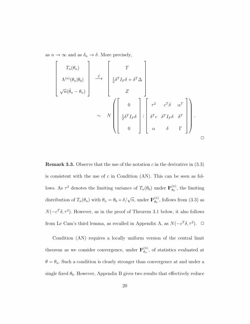
as n→∞ and as δn → δ. More precisely,Tn(θn)

Λ(n)(θn|θ0)√n(θn − θn)

L−→

T

12δT IF δ + δT∆

Z

∼ N

0

12δT IF δ

0

;

τ 2 cT δ αT

δT c δT IF δ δT

α δ Γ

.

2

Remark 3.3. Observe that the use of the notation c in the derivative in (3.3)

is consistent with the use of c in Condition (AN). This can be seen as fol-

lows. As τ 2 denotes the limiting variance of Tn(θ0) under IP(n)θ0

, the limiting

distribution of Tn(θn) with θn = θ0 + δ/√n, under IP

(n)θ0

, follows from (3.3) as

N(−cT δ, τ 2). However, as in the proof of Theorem 3.1 below, it also follows

from Le Cam’s third lemma, as recalled in Appendix A, as N(−cT δ, τ 2). 2

Condition (AN) requires a locally uniform version of the central limit

theorem as we consider convergence, under IP(n)θn

, of statistics evaluated at

θ = θn. Such a condition is clearly stronger than convergence at and under a

single fixed θ0. However, Appendix B gives two results that effectively reduce

20

the technical burden to an analysis of Tn(θ0) and√n(θn − θ0

)under IP

(n)θ0

only. These results are useful in both applications we consider.

Condition (AN) for the Binary Choice model: We consider the situa-

tion where θ is estimated using maximum likelihood, so that√n(θn − θ0) =

IF (θ0)−1∆(n)(θ0)+oIP(1). Using Proposition B.2, Condition (AN) follows from

Condition (ULAN) as far as Λ(n)(θn|θ0) and√n(θn − θn) are concerned.

Clearly, we have Γ = I−1F and α = Γc. Concerning the innovation-based

statistic Proposition B.1 applies.Using maximum likelihood implies Γ = I−1F

and Γc = α. Finally, α itself follows from

α = limn→∞

Covθ0

{√n(θn − θ0), T τn (θ0)

}(3.5)

= I−1F limn→∞

n

2

−1

n∑l=1

n∑i=1

i−1∑j=1

Cov{εGl Xl, 4I{εGi (θ) < εGj (θ), Zi < Zj} − 1

}

= 4I−1F limn→∞

n

2

−1

n∑i=1

i−1∑j=1

E(εGi Xi + εGj Xj

)I{εGi (θ) < εGj (θ), Zi < Zj}.

Further simplification of this expression is not necessary as it is easily esti-

mated consistently. 2

Condition (AN) for the Dynamic Volatility model: For condition-

21

ally heteroskedastic models, the QMLE estimator θn based on an assumed

Gaussian distribution for the innovations εt is a popular choice. For the

GARCH(1,1) model, Lumsdaine (1996) establishes consistency and asymp-

totic normality of this estimator under conditions implying the ones imposed

above. Her results essentially also establish (3.6) below. Recently, Berkes and

Horvath (2004) have improved upon these results showing, for GARCH(p,q)

processes, an asymptotically linear representation (B.4) for given θ:

√n(θn−θ) = −A(θ)−1

1√n

n∑t=1

1

4

(1− Y 2

t

σ2t−1(θ)

)∂

∂θlog σ2

t−1(θ)+oIP(1), (3.6)

under IP(n)θ . More precisely, (3.6) follows from their result (4.18) which, as

noted in the proof of their Theorem 2.1 is also valid for θn, applied to their

Example 2.1. From the representation (3.6) one finds the asymptotic variance

of the QMLE estimator as

Γ = Γ(θ) =κε − 1

4A(θ)−1, (3.7)

with κε = Eε4t (compared to Theorem 1.2 in Berkes and Horvath, 2004).

These results can be reinforced to obtain an estimator that actually sat-

isfies the local uniformity in Condition (AN) if (B.5) holds. While neither

Lumsdaine (1996) nor Berkes and Horvath (2004) explicitly mention (B.5),

their results allow us to invoke Proposition B.2 as the following lemma shows.

22

Lemma 3.1. For the GARCH(p, q) model, (B.5) holds for the Gaussian

QMLE estimator with

ψt(θ) = −A(θ)−11− ε2t (θ)

4

∂

∂θlog σ2

t−1(θ).

Proof. First of all note that A(θ) is invertible and continuous by applying

the mean-value theorem and using Lemma 3.6 in Berkes and Horvath (2004).

As a result, it suffices to study, for local alternatives θn to θ0,

1√n

n∑t=1

{1− ε2t−1(θn)

4

∂

∂θlog σ2

t−1(θn)−1− ε2t−1(θ0)

4

∂

∂θlog σ2

t−1(θ0)

},

(3.8)

under IP(n)θ0

. Consider a given element θ(j) of the vector θ. Applying Taylor’s

theorem to (3.8) we find, for the element corresponding to θ(j),(1

n

n∑t=1

ε2t (θ′n)

4

∂

∂θlog σ2

t−1(θ′n)

∂

∂θTlog σ2

t−1(θ′n) +

1− ε2t (θ′n)

4

∂2

∂θ∂θTlog σ2

t−1(θ′n)

)×√n(θn − θ0),

with θ′n on the line segment from θ0 to θn. Given the boundedness of√nθn−

θ0), it suffices to show that the term in parentheses converges to A(θ0). This,

however, follows from Lemma 4.4 in Berkes and Horvath (2004).

This shows that, with respect to the initial estimator θn, Condition (AN)

is indeed satisfied. With respect to the log-likelihood, as mentioned before,

23

Condition (AN) follows immediately from Condition (ULAN) and with re-

spect to the runs statistic, Proposition B.1 applies once more. 2

3.2 Size of residual-based tests

We now state and prove, in an informal way, the main result of the paper.

All statements will be made precise in Section 4.

Theorem 3.1. Under the Conditions (ULAN) and (AN) and in a way that

will be made precise in Section 4, we have, for the residual-based statistic

Tn(θn),

Tn(θn)L−→ N

(0, τ 2 + (α− Γc)TΓ−1(α− Γc)− αTΓ−1α

)(3.9)

= N(0, τ 2 + cTΓc− 2αT c

),

under IP(n)θn

, as n→∞.

Proof. (Intuition) Introduce the distributionT

∆

Z

∼ N

0,

τ 2 cT αT

c IF Ik

α Ik Γ

. (3.10)

24

where Ik denotes the k × k identity matrix. From Condition (AN), applied

with θn replaced by θn + δ/√n and using Condition (ULAN), we have for all

δ ∈ IRk, under IP(n)

θn+δ/√n

and as n→∞,Tn(θn + δ/

√n)

Λ(n)(θn|θn + δ/√n)

√n(θn − θn − δ/

√n)

L−→

T

−12δT IF δ − δT∆

Z

,while, as a consequence of Le Cam’s third lemma, the same vector converges

under IP(n)θn

to T − cT δ

+12δT IF δ − δT∆

Z − δ

.The quantity of interest can now be written, for t ∈ IR,

IP(n)θn

{Tn(θn) ≤ t

}=

∫δ∈IRk

IP(n)θn

{Tn(θn) ≤ t|θn = θn + δ/

√n}

dIP(n)θn

{θn ≤ θn + δ/

√n}

=

∫δ∈IRk

IP(n)θn

{Tn(θn + δ/

√n) ≤ t|

√n(θn − θn) = δ

}dIP

(n)θn

{√n(θn − θn) ≤ δ

}→

∫δ∈IRk

IP{T − cT δ ≤ t|Z = δ

}dIP {Z ≤ δ}

=

∫δ∈IRk

Φ

(t+ (c− Γ−1α)T δ√τ 2 − αTΓ−1α

)dIP {Z ≤ δ} ,

where Φ denotes the cumulative distribution function of the standard normal

distribution and we used the result that, conditionally on Z = z, T has

25

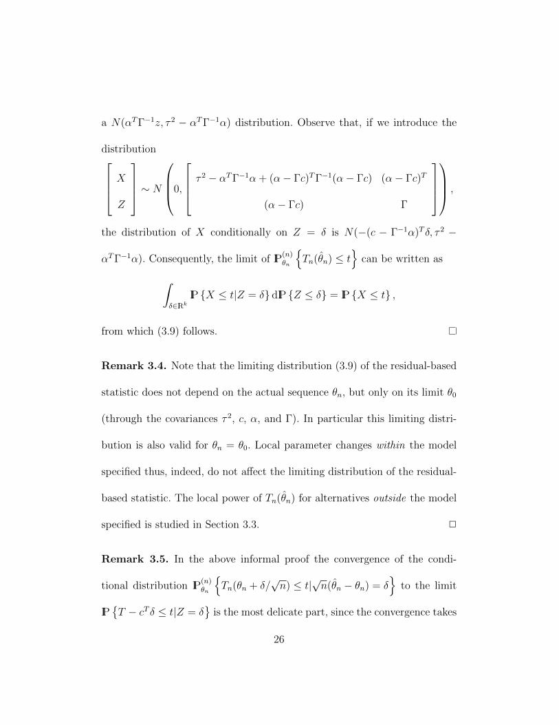
a N(αTΓ−1z, τ 2 − αTΓ−1α) distribution. Observe that, if we introduce the

distribution X

Z

∼ N

0,

τ 2 − αTΓ−1α + (α− Γc)TΓ−1(α− Γc) (α− Γc)T

(α− Γc) Γ

,

the distribution of X conditionally on Z = δ is N(−(c − Γ−1α)T δ, τ 2 −

αTΓ−1α). Consequently, the limit of IP(n)θn

{Tn(θn) ≤ t

}can be written as

∫δ∈IRk

IP {X ≤ t|Z = δ} dIP {Z ≤ δ} = IP {X ≤ t} ,

from which (3.9) follows.

Remark 3.4. Note that the limiting distribution (3.9) of the residual-based

statistic does not depend on the actual sequence θn, but only on its limit θ0

(through the covariances τ 2, c, α, and Γ). In particular this limiting distri-

bution is also valid for θn = θ0. Local parameter changes within the model

specified thus, indeed, do not affect the limiting distribution of the residual-

based statistic. The local power of Tn(θn) for alternatives outside the model

specified is studied in Section 3.3. 2

Remark 3.5. In the above informal proof the convergence of the condi-

tional distribution IP(n)θn

{Tn(θn + δ/

√n) ≤ t|

√n(θn − θn) = δ

}to the limit

IP{T − cT δ ≤ t|Z = δ

}is the most delicate part, since the convergence takes

26

place in the conditioning event as well. A formalization of such a convergence

would require conditions under which a conditional probability or expecta-

tion is continuous with respect to the conditioning event. This question has

been studied in the literature by introducing various topologies on the space

of conditioning σ-fields. A good reference is the paper by Cotter (1986) that

compares some topologies. From our point of interest, Cotter (1986) essen-

tially shows that the required continuity property only holds for discrete

probability distributions. Indeed, we formalize Theorem 3.1 by discretizing

the estimator θn appropriately. See Section 4 for details. 2

Remark 3.6. Theorem 3.1 has been stated for univariate statistics Tn(θ),

but can easily be extended to the multivariate case using the Cramer-Wold

device. In such a multivariate setting τ 2, c, and α in Condition (AN) are

matrices. By taking arbitrary linear combinations of the components of Tn

and applying the univariate version of Theorem 3.1, we find that the same

limiting distribution (3.9) holds with τ 2 replaced by the limiting variance

matrix of Tn, c the limiting covariance matrix between the statistic and the

central sequence, and α the limiting covariance matrix between the statistic

and the estimator used. 2

Size of Kendall’s tau for the Binary Choice model: Recall that the lim-

27

iting variance of the innovation-based Kendall’s tau is τ 2 = 4/9. In order to

derive the appropriate variance correction when calculating Kendall’s tau us-

ing generalized residuals (calculated on the basis of the maximum likelihood

estimator θ(ML)n ), we adopt Theorem 3.1. As α = Γc, applying Theorem 3.1

we obtain, under the null hypothesis of no omitted variables,

T τn (θ(ML)n )

L−→ N

(0;

4

9− αT IFα

).

This nonparametric test for omitted variables in the binary choice model

has not been considered before in the literature. We provide this application

to show that its limiting distribution is easily derived in the framework we

propagate. 2

Size of runs test for the Dynamic Volatility model: Without going

through all the calculations in detail, observe that in this case c = 0 since

EI{εt < 0} (1 + εtf′(εt)/f(εt)) =

1

2+

∫ 0

x=−∞xf ′(x)dx

=1

2−∫ 0

x=−∞f(x)dx = 0,

which implies

Et−1[I{εt < 0} − I{εt−1 < 0}]2 (1 + εtf′(εt)/f(εt)) = 0.

28

Consequently, using Theorem 3.1, the asymptotic covariance of the Wald-

Wolfowitz runs test for symmetry need not be adapted to estimation error

when applied to the residuals of dynamic volatility models. 2

If we think of canonical applications, Tn(θ) represents a test statistic for

distributional or time series properties of some innovations in the model,

while Tn(θ) denotes the same statistic applied to estimated residuals in the

model. Theorem 3.1 shows that replacing innovations by residuals may leave

the asymptotic variance of the test statistic unchanged, increase it, or de-

crease it, depending on the value of (α − Γc)TΓ−1(α − Γc) as compared to

αTΓ−1α. Several special cases can occur.

First, if c = 0, the residual-based statistic has the same asymptotic vari-

ance as the statistic based on the true innovations. In particular, no adap-

tation is necessary in critical values in order to guarantee the appropriate

asymptotic size of the test when applied to estimated residuals. However,

the power of the residual-based test Tn(θn) may be different from that of the

innovation-based test Tn(θn) (see Section 3.3 for details). Recall that, under

c = 0, the test statistic and the central sequence are asymptotically indepen-

dent. As a result, the distribution of the test statistic Tn(θ0) is insensitive

29

to local changes in the parameter θ. In particular, the asymptotic distribu-

tion of Tn(θ0) is the same under all probability distributions IP(n)θn

, whatever

the local parameter sequence θn. Or, equivalently in our setup, the asymp-

totic distribution of Tn(θn) under IP(n)θ0

is the same for each local sequence

θn. As estimated parameter values θ differ from θ0 in the order of magnitude

of 1/√n, these remarks apparently carry over to the residual-based statistic.

Our runs-based test for symmetry in the dynamic volatility model falls under

this scheme.

A second special case occurs if α = Γc. This happens, for instance, when

the initial estimator θn is efficient (as in that case Γ = I−1F and α = I−1F c). In

such situation, the limiting variance of the residual-based statistic is smaller

than the limiting variance of the statistic applied to the true innovations, with

strict inequality if α 6= 0. Pierce (1982) restricts attention to this efficient

initial estimator case and, imposing a differentiability condition on Tn(θ),

finds the same reduction in the limiting variance. This occurs, for instance,

in our application of omitted variables tests in the binary choice model.

Finally, it might be that α = 0. In this case the limiting variance of the

residual statistic becomes τ 2 + cTΓc ≥ τ 2. When α = 0, the test statistic

Tn(θ) is asymptotically independent from the estimator θn and a test based

30

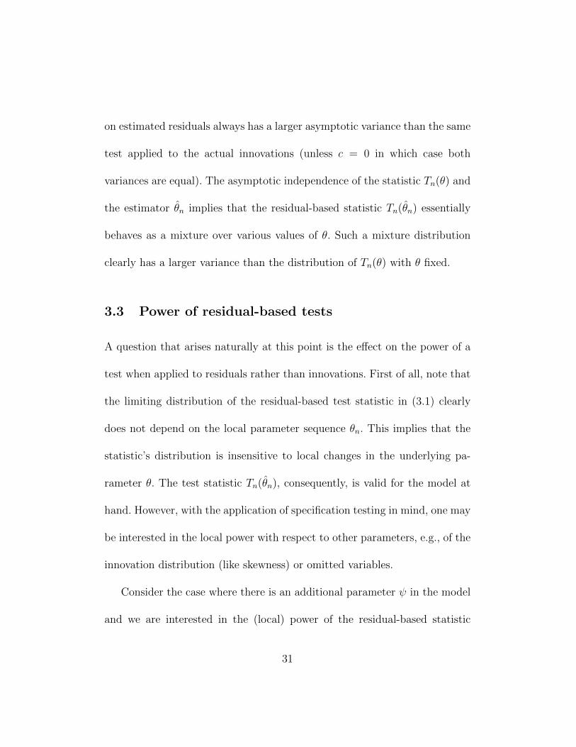
on estimated residuals always has a larger asymptotic variance than the same

test applied to the actual innovations (unless c = 0 in which case both

variances are equal). The asymptotic independence of the statistic Tn(θ) and

the estimator θn implies that the residual-based statistic Tn(θn) essentially

behaves as a mixture over various values of θ. Such a mixture distribution

clearly has a larger variance than the distribution of Tn(θ) with θ fixed.

3.3 Power of residual-based tests

A question that arises naturally at this point is the effect on the power of a

test when applied to residuals rather than innovations. First of all, note that

the limiting distribution of the residual-based test statistic in (3.1) clearly

does not depend on the local parameter sequence θn. This implies that the

statistic’s distribution is insensitive to local changes in the underlying pa-

rameter θ. The test statistic Tn(θn), consequently, is valid for the model at

hand. However, with the application of specification testing in mind, one may

be interested in the local power with respect to other parameters, e.g., of the

innovation distribution (like skewness) or omitted variables.

Consider the case where there is an additional parameter ψ in the model

and we are interested in the (local) power of the residual-based statistic

31

Tn(θn) with respect to this parameter. The model now consists of a set of

probability measures {IP(n)θ,ψ : θ ∈ Θ, ψ ∈ Ψ}. For ease of notation we assume

that the original model is obtained by setting ψ = 0, i.e., IP(n)θ,0 = IP

(n)θ .

As before, fix θ0 ∈ Θ and consider the local parametrization (θn, ψn) =

(θ0 + δ/√n, 0 + η/

√n). Introduce the log-likelihood

Λ(n)(ψn|0) = logdIP

(n)θ0,ψn

dIP(n)θ0,0

,

with respect to the parameter ψ. We are interested in the behavior of our

test statistic Tn(θn) under IP(n)θ0,ψn

. Assume that Condition (ULAN) is satisfied

jointly in θ and ψ. Moreover, assume the equivalent of Condition (AN) under

ψ = 0, i.e., under IP(n)θn,0

and as n→∞,

Tn(θn)

Λ(n)(θn|θ0)√n(θn − θn

)Λ(n)(ψn|0)

L−→

T

12δT IF δ + δT∆

Z

−12ηT IPη + δT IFPη + ηT ∆

(3.11)

∼ N

0

12δT IF δ

0

−12ηT IPη + δT IFPη

,

τ 2 cT δ αT dTη

δT c δT IF δ δT δT IFPη

α δ Γ BTη

ηTd ηT IFP δ ηTB ηT IPη

.

32

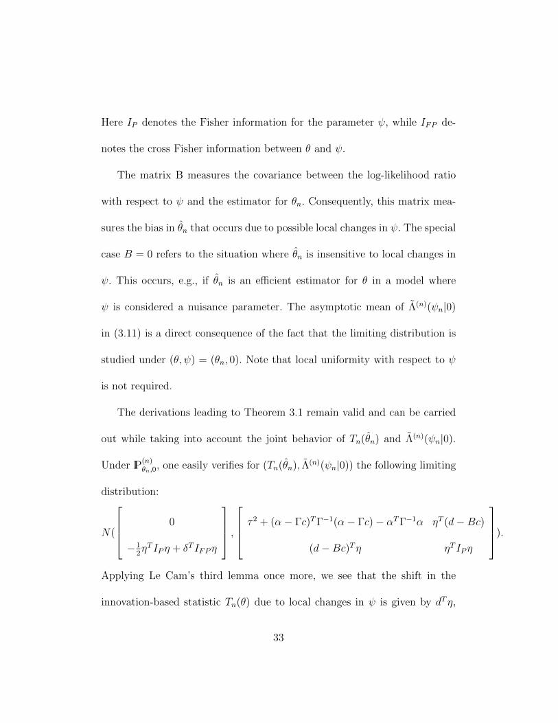
Here IP denotes the Fisher information for the parameter ψ, while IFP de-

notes the cross Fisher information between θ and ψ.

The matrix B measures the covariance between the log-likelihood ratio

with respect to ψ and the estimator for θn. Consequently, this matrix mea-

sures the bias in θn that occurs due to possible local changes in ψ. The special

case B = 0 refers to the situation where θn is insensitive to local changes in

ψ. This occurs, e.g., if θn is an efficient estimator for θ in a model where

ψ is considered a nuisance parameter. The asymptotic mean of Λ(n)(ψn|0)

in (3.11) is a direct consequence of the fact that the limiting distribution is

studied under (θ, ψ) = (θn, 0). Note that local uniformity with respect to ψ

is not required.

The derivations leading to Theorem 3.1 remain valid and can be carried

out while taking into account the joint behavior of Tn(θn) and Λ(n)(ψn|0).

Under IP(n)θn,0

, one easily verifies for (Tn(θn), Λ(n)(ψn|0)) the following limiting

distribution:

N(

0

−12ηT IPη + δT IFPη

, τ 2 + (α− Γc)TΓ−1(α− Γc)− αTΓ−1α ηT (d−Bc)

(d−Bc)Tη ηT IPη

).

Applying Le Cam’s third lemma once more, we see that the shift in the

innovation-based statistic Tn(θ) due to local changes in ψ is given by dTη,

33

while the same local change in ψ induces a shift of size (d − Bc)Tη in the

residual-based statistic Tn(θ). Consequently, while the local power of the

innovation-based static Tn(θ) is determined by d/τ , that of the residual-based

statistic Tn(θn) is determined by

(d−Bc)/√τ 2 + (α− Γc)TΓ−1(α− Γc)− αTΓ−1α. (3.12)

In case c = 0, we find that not only the size of the residual-based statistic

is unaltered, but also that its power equals that of the innovation-based statis-

tic. In the special case that B = 0, we thus find that the power against local

changes in ψ in the residual-based statistic decreases, remains unchanged,

or increases as the limiting variance of the residual-based statistic increases,

remains unchanged, or decreases, respectively. It may thus very well be the

case that residual-based statistics have more power against certain local al-

ternatives than the same statistic applied to actual innovations.

Alternatively, the results in this section can be interpreted in terms of

specification testing with locally misspecified alternatives much in the same

spirit as Bera and Yoon (1993). Bera and Yoon (1993) derive a correction

to standard LM tests which makes them insensitive to local misspecifica-

tion. Not surprisingly, this correction exactly contains the covariance term

B, which is Jψφ in their Formula (3.2).

34

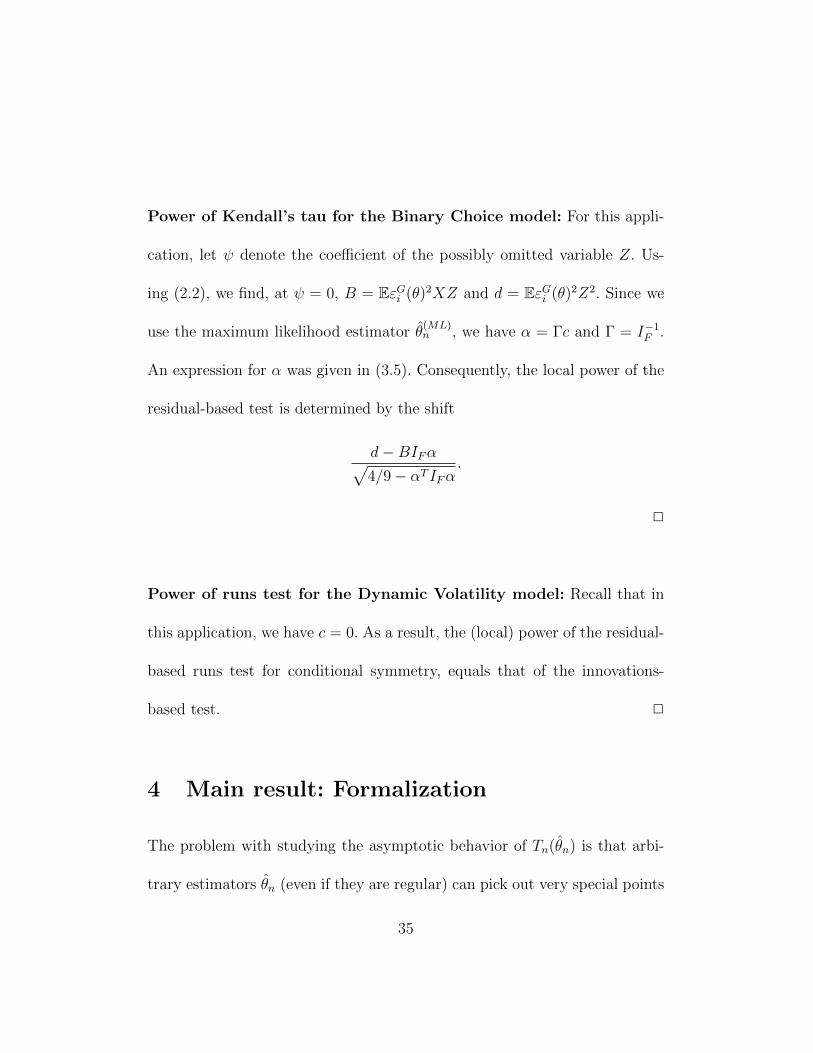
Power of Kendall’s tau for the Binary Choice model: For this appli-

cation, let ψ denote the coefficient of the possibly omitted variable Z. Us-

ing (2.2), we find, at ψ = 0, B = EεGi (θ)2XZ and d = EεGi (θ)2Z2. Since we

use the maximum likelihood estimator θ(ML)n , we have α = Γc and Γ = I−1F .

An expression for α was given in (3.5). Consequently, the local power of the

residual-based test is determined by the shift

d−BIFα√4/9− αT IFα

.

2

Power of runs test for the Dynamic Volatility model: Recall that in

this application, we have c = 0. As a result, the (local) power of the residual-

based runs test for conditional symmetry, equals that of the innovations-

based test. 2

4 Main result: Formalization

The problem with studying the asymptotic behavior of Tn(θn) is that arbi-

trary estimators θn (even if they are regular) can pick out very special points

35

of the parameter space. Without strong uniformity conditions on the behav-

ior of Tn(θ) as a function of θ, the residual statistic Tn(θn) could behave in an

erratic way. We solve this problem by discretizing the estimator θn. This is a

well-known technical trick due to Le Cam. We introduce this approach now

and study the behavior of the statistic based on the discretized estimated

parameter.

The discretized estimator θn is obtained by rounding the original esti-

mator θn to the nearest midpoint in a regular grid of cubes. To be precise,

consider a grid of cubes in IRk with sides of length d/√n. We call d the

discretization constant. Then θn is the estimator obtained by taking the

midpoint of the cube to which θn belongs. To formalize this even further,

introduce the function r : IRk → ZZk which arithmetically rounds each of the

components of the input vector to the nearest integer. Then, we may write

θn = dr(√nθn/d)/

√n. Our interest lies in the asymptotic behavior of Tn(θn)

for small d. We first study the behavior of θn in the following lemma.

Lemma 4.1. Let the discretization constant d > 0 be given. Define the “dis-

cretized truth” θn = dr(√nθ0/d)/

√n. Then

√n(θn − θn) is degenerated on

{dj : j ∈ ZZk}. Moreover, for δn → δ as n→∞, we have

IP(n)

θn+δn/√n

{√n(θn − θn) = dj

}→ IP

{N(δ − dj,Γ) ∈ (−d

2ι,d

2ι]

}, (4.1)

36

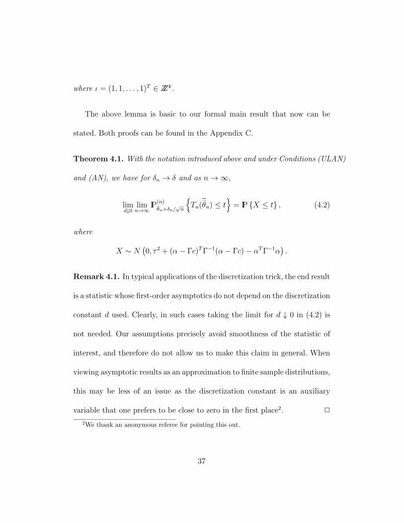
where ι = (1, 1, . . . , 1)T ∈ ZZk.

The above lemma is basic to our formal main result that now can be

stated. Both proofs can be found in the Appendix C.

Theorem 4.1. With the notation introduced above and under Conditions (ULAN)

and (AN), we have for δn → δ and as n→∞,

limd↓0

limn→∞

IP(n)

θn+δn/√n

{Tn(θn) ≤ t

}= IP {X ≤ t} , (4.2)

where

X ∼ N(0, τ 2 + (α− Γc)TΓ−1(α− Γc)− αTΓ−1α

).

Remark 4.1. In typical applications of the discretization trick, the end result

is a statistic whose first-order asymptotics do not depend on the discretization

constant d used. Clearly, in such cases taking the limit for d ↓ 0 in (4.2) is

not needed. Our assumptions precisely avoid smoothness of the statistic of

interest, and therefore do not allow us to make this claim in general. When

viewing asymptotic results as an approximation to finite sample distributions,

this may be less of an issue as the discretization constant is an auxiliary

variable that one prefers to be close to zero in the first place2. 2

2We thank an anonymous referee for pointing this out.

37

Remark 4.2. As for the informal derivations in Section 3, the above proof

is strongly based on a conditioning argument with respect to the value of the

estimator θn, or, more precisely, that of the local estimation error√n(θn−θn).

This leads one to believe that it is meaningfully possible to derive LAN con-

ditions for conditional distributions, where the conditioning event is the value

of some estimation error. The authors of the present paper have, however,

not seen any results in this direction. 2

5 Conclusions

This paper introduces a novel asymptotic analysis of residuals-based statistics

in a Gaussian limiting framework: The models under consideration are as-

sumed to be locally asymptotically normal (LAN), the statistics being studied

have limiting normal distributions, and the estimators under consideration

are√n-consistent and asymptotically normal. In our approach we do not

explicitly require any smoothness of the statistics of interest with respect

to the nuisance parameter, but we do impose a locally uniform convergence

condition that is satisfied for residual-based statistics. We apply this method

to derive several new results. For example, we present a new omitted vari-

38

able specification test for limited dependent variable models and provide its

asymptotic distribution. Our method is also useful for deriving the asymp-

totic distribution of two-step estimators and nonparametric tests.

The method proposed in the paper can be extended in several interesting

directions. First of all, while the Gaussian context has many applications for

residual-based testing in econometric models, our method essentially builds

on Le Cam’s third lemma which is not restricted to Gaussian situations. In

particular, limiting χ2 distributions can be handled easily using the same

techniques. Also, in case the model of interest is not specified in terms of

likelihoods but in terms of moments (like in GMM settings), the same ideas

can be applied (see Andreou and Werker, 2009, for further details). Local de-

viations of the moment conditions can be cast in likelihood terms such that

our method still applies. Last but not least, our approach may also represent

the foundations for an alternative to the derivation of asymptotic distribu-

tions of non-Gaussian statistics as, for instance, in Locally Asymptotically

Mixed Normal (LAMN) models.

Acknowledgements

Part of this research was completed when the first author held a Marie

Curie fellowship at Tilburg University (MCFI-2000-01645) and while both

39

authors were visiting the Statistical and Applied Mathematical Sciences In-

stitute (SAMSI). The first author acknowledges support of the European Re-

search Council under the European Community FP7/2008-2012 ERC grant

209116. The second author also acknowledges support from Mik. Comments

by two anonymous referees, Anil Bera, Christel Bouquiaux, Rob Engle, Eric

Ghysels, Lajos Horvath, Nour Meddahi, Bertrand Melenberg, Werner Ploberger,

Eric Renault, Enrique Sentana, conference participants at the ESEM 2004,

MEG 2004, and NBER time series 2004 conferences, and seminar participants

at the London School of Economics, Universite de Montreal, and Tilburg

University are kindly acknowledged.

A Le Cam’s third Lemma

Le Cam’s third lemma is discussed in several modern books on asymp-

totic statistics, e.g., Hajek and Sidak (1967), Le Cam and Yang (1990),

Bickel et al. (1993), or van der Vaart (1998). We recall it in its best-known

form, i.e., for asymptotically normal distributions. Consider two sequences

of probability measures(

Q(n))∞n=1

and(

IP(n))∞n=1

defined on the common

measurable spaces(X(n),X (n)

)∞n=1

. Assume that the log-likelihood ratios

40

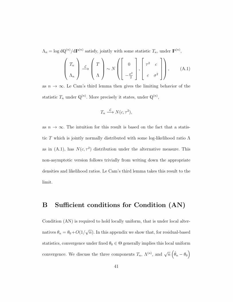
Λn = log dQ(n)/dIP(n) satisfy, jointly with some statistic Tn, under IP(n), Tn

Λn

L−→

T

Λ

∼ N

0

−σ2

2

, τ 2 c

c σ2

, (A.1)

as n → ∞. Le Cam’s third lemma then gives the limiting behavior of the

statistic Tn under Q(n). More precisely it states, under Q(n),

TnL−→ N(c, τ 2),

as n → ∞. The intuition for this result is based on the fact that a statis-

tic T which is jointly normally distributed with some log-likelihood ratio Λ

as in (A.1), has N(c, τ 2) distribution under the alternative measure. This

non-asymptotic version follows trivially from writing down the appropriate

densities and likelihood ratios. Le Cam’s third lemma takes this result to the

limit.

B Sufficient conditions for Condition (AN)

Condition (AN) is required to hold locally uniform, that is under local alter-

natives θn = θ0+O(1/√n). In this appendix we show that, for residual-based

statistics, convergence under fixed θ0 ∈ Θ generally implies this local uniform

convergence. We discuss the three components Tn, Λ(n), and√n(θn − θ0

)41

in Condition (AN) separately, but, using the Cramer-Wold device, the argu-

ments can easily be combined to prove locally uniform joint convergence.

First, consider the test statistic Tn. Recall that, in our framework, Tn

refers to a residual-based statistic used for specification testing. In such case,

we can generally write

Tn(θ) = T (ε1(θ), . . . εn(θ)) , (B.1)

where the innovations εt(θ) are i.i.d., under IP(n)θ , and T is some given func-

tion. It is not excluded that Tn depends on some exogenous variables as well.

Assuming appropriate centering and scaling, such statistics often satisfy an

asymptotic representation, for given θ = θ0,

Tn(θ0) =1√n

n∑t=1

τ (εt(θ0), . . . , εt−l(θ0)) + op(1), (B.2)

under IP(n)θ0

, for some function τ : IRl → IR such that a (l + 1-dependent)

central limit theorem can be applied to (B.2). We now have the following

simple but useful result, which is invoked in all applications mentioned in

this paper.

Proposition B.1. Suppose that the statistic Tn(θ) can be written as in (B.1)

and satisfies (B.2). Then, for local alternatives θn to θ0, we have, under IP(n)θn

,

Tn(θn) =1√n

n∑t=1

τ (εt(θn), . . . , εt−l(θn)) + op(1). (B.3)

42

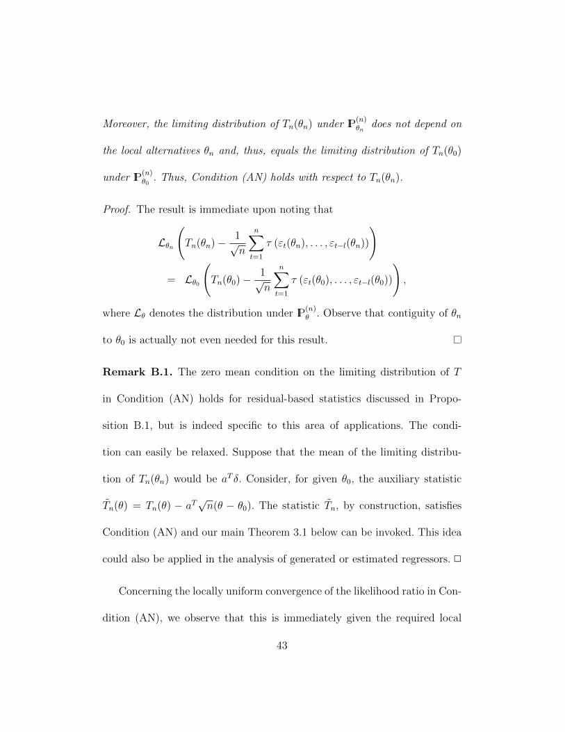
Moreover, the limiting distribution of Tn(θn) under IP(n)θn

does not depend on

the local alternatives θn and, thus, equals the limiting distribution of Tn(θ0)

under IP(n)θ0

. Thus, Condition (AN) holds with respect to Tn(θn).

Proof. The result is immediate upon noting that

Lθn

(Tn(θn)− 1√

n

n∑t=1

τ (εt(θn), . . . , εt−l(θn))

)

= Lθ0

(Tn(θ0)−

1√n

n∑t=1

τ (εt(θ0), . . . , εt−l(θ0))

),

where Lθ denotes the distribution under IP(n)θ . Observe that contiguity of θn

to θ0 is actually not even needed for this result.

Remark B.1. The zero mean condition on the limiting distribution of T

in Condition (AN) holds for residual-based statistics discussed in Propo-

sition B.1, but is indeed specific to this area of applications. The condi-

tion can easily be relaxed. Suppose that the mean of the limiting distribu-

tion of Tn(θn) would be aT δ. Consider, for given θ0, the auxiliary statistic

Tn(θ) = Tn(θ) − aT√n(θ − θ0). The statistic Tn, by construction, satisfies

Condition (AN) and our main Theorem 3.1 below can be invoked. This idea

could also be applied in the analysis of generated or estimated regressors. 2

Concerning the locally uniform convergence of the likelihood ratio in Con-

dition (AN), we observe that this is immediately given the required local

43

uniformity in Condition (ULAN). Merely imposing a LAN condition would,

together with the local uniformity required in Condition (AN), essentially im-

ply ULAN. In order to be precise about the scope of our results, we impose

condition ULAN from the start.

Concerning the estimator θn, Condition (AN) imposes that the limiting

distribution, in particular its mean, of√n(θn − θn

), under IP

(n)θn

, does not de-

pend on the local alternatives θn and, hence, equals the limit of√n(θn − θ0

),

under IP(n)θ0

. This is to say that the estimator is regular in the sense of Bickel

et al. (1993), page 18, or van der Vaart (1998), page 115. Regularity also

implies that the asymptotic covariance between the estimator and the cen-

tral sequence is the k × k identity matrix Ik. In particular, the convolution

theorem stating that asymptotic variances of estimators are always larger

than the inverse of the Fisher information only applies to regular estimators;

regularity is used to rule out superefficient estimators. Estimators that sat-

isfy an asymptotically linear representation can often be transformed into

regular estimators. This is formalized in the proposition below, whose proof

follows easily along the lines of, e.g., van der Vaart (1998), Section 5.7.

Proposition B.2. Maintaining the Condition (ULAN), consider an estima-

44

tor θn that satisfies, under IP(n)θ0

, the asymptotic representation

√n(θn − θ0

)=

1√n

n∑t=1

ψt(θ0) + op(1), (B.4)

with ψt some influence function that satisfies, still under IP(n)θ0

,

1√n

n∑t=1

ψt(θ0)L−→ N(0,Γ).

Moreover, assume, for local alternatives θn to θ0,

1√n

n∑t=1

ψt(θn)− 1√n

n∑t=1

ψt(θ0) = −√n (θn − θ0) + op(1), (B.5)

under IP(n)θ0

. Then, we can construct an estimator θn such that, under IP(n)θn

,

√n(θn − θn

)=

1√n

n∑t=1

ψt(θn) + op(1), (B.6)

and, under IP(n)θ0

,√n(θn − θn

)= op(1).

Proof. The construction follows the ideas in, e.g., van der Vaart (1998), Sec-

tion 5.7. First of all, discretize the estimator θn as described in Section 4.

Denote this estimator θn. Define the estimator

θn := θn +1√n

n∑t=1

ψt(θn). (B.7)

Observe, for local alternatives θn and by applying (B.5) twice,

1√n

n∑t=1

ψt(θn)− 1√n

n∑t=1

ψt(θn) = −√n(θn − θn

)+ op(1). (B.8)

45

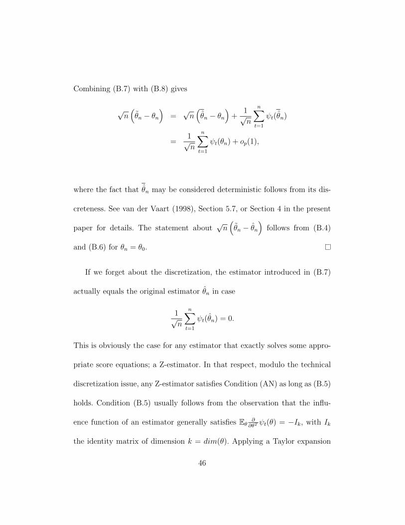
Combining (B.7) with (B.8) gives

√n(θn − θn

)=√n(θn − θn

)+

1√n

n∑t=1

ψt(θn)

=1√n

n∑t=1

ψt(θn) + op(1),

where the fact that θn may be considered deterministic follows from its dis-

creteness. See van der Vaart (1998), Section 5.7, or Section 4 in the present

paper for details. The statement about√n(θn − θn

)follows from (B.4)

and (B.6) for θn = θ0.

If we forget about the discretization, the estimator introduced in (B.7)

actually equals the original estimator θn in case

1√n

n∑t=1

ψt(θn) = 0.

This is obviously the case for any estimator that exactly solves some appro-

priate score equations; a Z-estimator. In that respect, modulo the technical

discretization issue, any Z-estimator satisfies Condition (AN) as long as (B.5)

holds. Condition (B.5) usually follows from the observation that the influ-

ence function of an estimator generally satisfies Eθ ∂∂θT

ψt(θ) = −Ik, with Ik

the identity matrix of dimension k = dim(θ). Applying a Taylor expansion

46

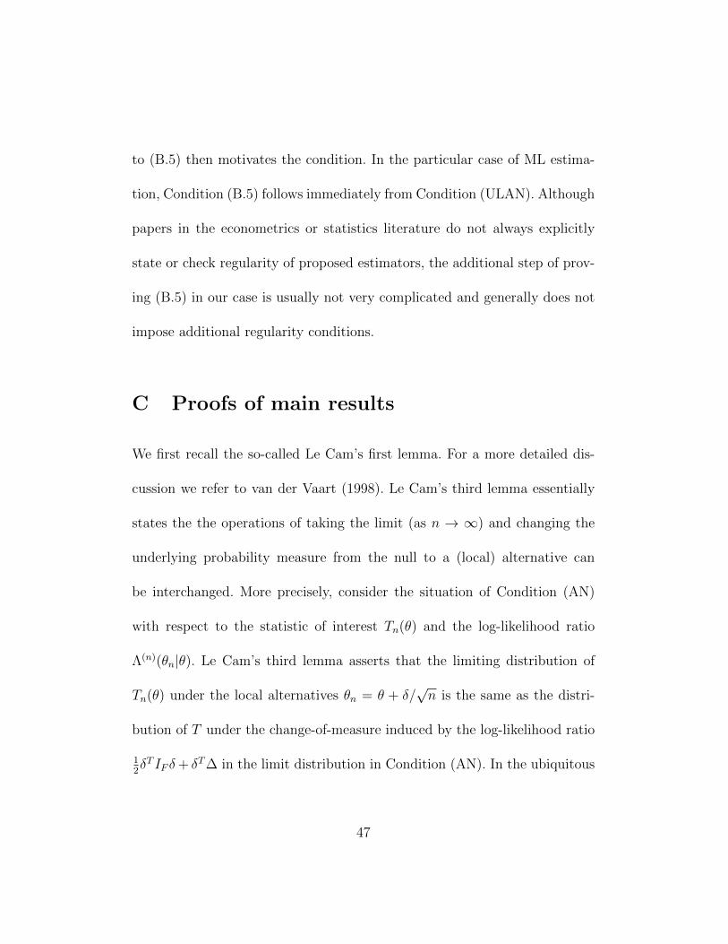
to (B.5) then motivates the condition. In the particular case of ML estima-

tion, Condition (B.5) follows immediately from Condition (ULAN). Although

papers in the econometrics or statistics literature do not always explicitly

state or check regularity of proposed estimators, the additional step of prov-

ing (B.5) in our case is usually not very complicated and generally does not

impose additional regularity conditions.

C Proofs of main results

We first recall the so-called Le Cam’s first lemma. For a more detailed dis-

cussion we refer to van der Vaart (1998). Le Cam’s third lemma essentially

states the the operations of taking the limit (as n → ∞) and changing the

underlying probability measure from the null to a (local) alternative can

be interchanged. More precisely, consider the situation of Condition (AN)

with respect to the statistic of interest Tn(θ) and the log-likelihood ratio

Λ(n)(θn|θ). Le Cam’s third lemma asserts that the limiting distribution of

Tn(θ) under the local alternatives θn = θ + δ/√n is the same as the distri-

bution of T under the change-of-measure induced by the log-likelihood ratio

12δT IF δ+ δT∆ in the limit distribution in Condition (AN). In the ubiquitous

47

case of a Gaussian limit distribution, the resulting limit is well-known to be

Gaussian with the same variance τ 2, but with a shift in the mean of size−cT δ.

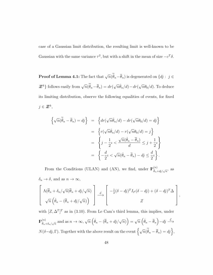
Proof of Lemma 4.1: The fact that√n(θn−θn) is degenerated on {dj : j ∈

ZZk} follows easily from√n(θn−θn) = dr(

√nθn/d)−dr(

√nθ0/d). To deduce

its limiting distribution, observe the following equalities of events, for fixed

j ∈ ZZk,

{√n(θn − θn) = dj

}=

{dr(√nθn/d)− dr(

√nθ0/d) = dj

}=

{r(√nθn/d)− r(

√nθ0/d) = j

}=

{j − 1

2ι <

√n(θn − θn)

d≤ j +

1

2ι

}

=

{−d

2ι <√n(θn − θn)− dj ≤ d

2ι

}.

From the Conditions (ULAN) and (AN), we find, under IP(n)

θn+dj/√n, as

δn → δ, and as n→∞, Λ(θn + δn/√n|θn + dj/

√n)

√n(θn − (θn + dj/

√n)) L−→

−12(δ − dj)T IF (δ − dj) + (δ − dj)T∆

Z

,with [Z,∆T ]T as in (3.10). From Le Cam’s third lemma, this implies, under

IP(n)

θn+δn/√n

and as n→∞,√n(θn − (θn + dj/

√n))

=√n(θn − θn

)−dj L−→

N(δ−dj,Γ). Together with the above result on the event{√

n(θn − θn) = dj}

,

48

the lemma now follows. 2

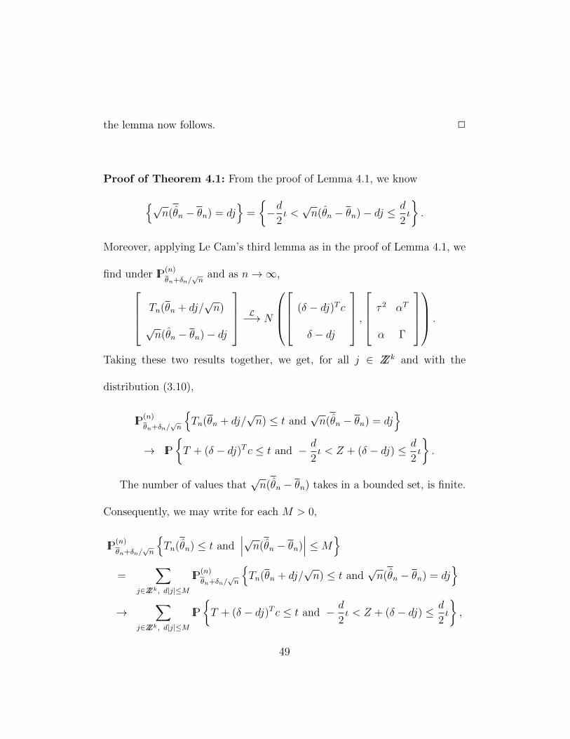
Proof of Theorem 4.1: From the proof of Lemma 4.1, we know

{√n(θn − θn) = dj

}=

{−d

2ι <√n(θn − θn)− dj ≤ d

2ι

}.

Moreover, applying Le Cam’s third lemma as in the proof of Lemma 4.1, we

find under IP(n)

θn+δn/√n

and as n→∞, Tn(θn + dj/√n)

√n(θn − θn)− dj

L−→ N

(δ − dj)T c

δ − dj

, τ 2 αT

α Γ

.

Taking these two results together, we get, for all j ∈ ZZk and with the

distribution (3.10),

IP(n)

θn+δn/√n

{Tn(θn + dj/

√n) ≤ t and

√n(θn − θn) = dj

}→ IP

{T + (δ − dj)T c ≤ t and − d

2ι < Z + (δ − dj) ≤ d

2ι

}.

The number of values that√n(θn − θn) takes in a bounded set, is finite.

Consequently, we may write for each M > 0,

IP(n)

θn+δn/√n

{Tn(θn) ≤ t and

∣∣∣√n(θn − θn)∣∣∣ ≤M

}=

∑j∈ZZk, d|j|≤M

IP(n)

θn+δn/√n

{Tn(θn + dj/

√n) ≤ t and

√n(θn − θn) = dj

}→

∑j∈ZZk, d|j|≤M

IP

{T + (δ − dj)T c ≤ t and − d

2ι < Z + (δ − dj) ≤ d

2ι

},

49

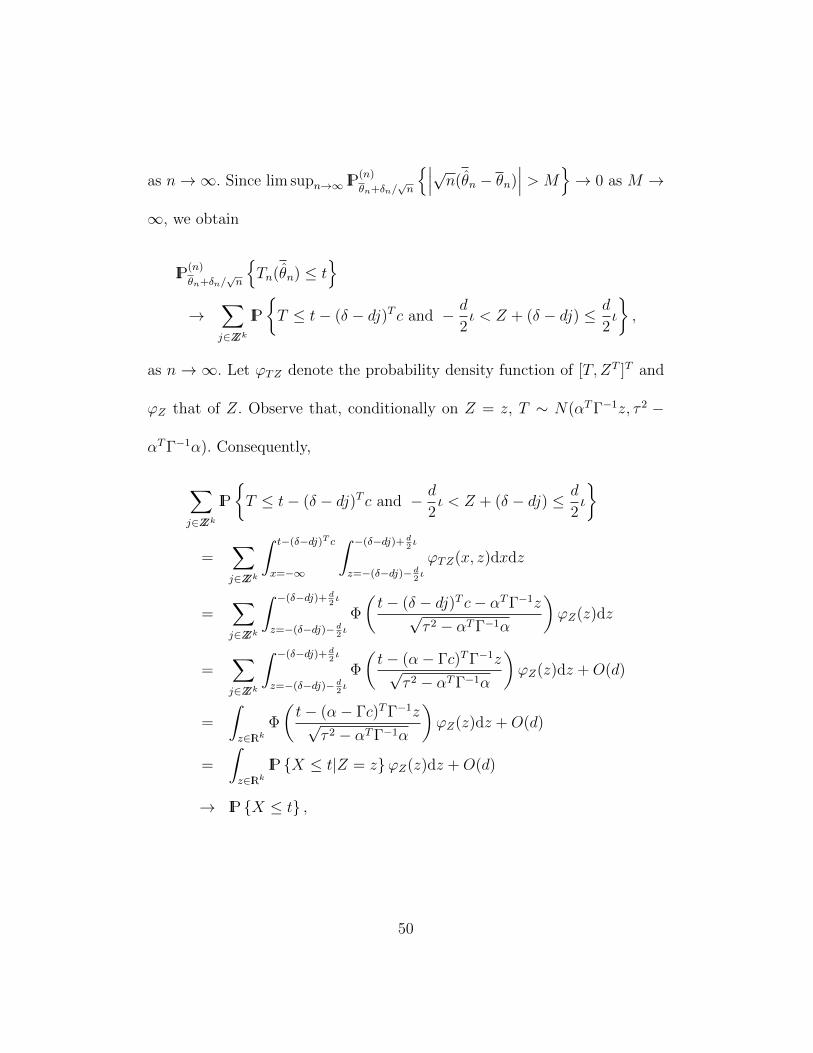
as n→∞. Since lim supn→∞ IP(n)

θn+δn/√n

{∣∣∣√n(θn − θn)∣∣∣ > M

}→ 0 as M →

∞, we obtain

IP(n)

θn+δn/√n

{Tn(θn) ≤ t

}→

∑j∈ZZk

IP

{T ≤ t− (δ − dj)T c and − d

2ι < Z + (δ − dj) ≤ d

2ι

},

as n → ∞. Let ϕTZ denote the probability density function of [T, ZT ]T and

ϕZ that of Z. Observe that, conditionally on Z = z, T ∼ N(αTΓ−1z, τ 2 −

αTΓ−1α). Consequently,

∑j∈ZZk

IP

{T ≤ t− (δ − dj)T c and − d

2ι < Z + (δ − dj) ≤ d

2ι

}

=∑j∈ZZk

∫ t−(δ−dj)T c

x=−∞

∫ −(δ−dj)+ d2ι

z=−(δ−dj)− d2ι

ϕTZ(x, z)dxdz

=∑j∈ZZk

∫ −(δ−dj)+ d2ι

z=−(δ−dj)− d2ι

Φ

(t− (δ − dj)T c− αTΓ−1z√

τ 2 − αTΓ−1α

)ϕZ(z)dz

=∑j∈ZZk

∫ −(δ−dj)+ d2ι

z=−(δ−dj)− d2ι

Φ

(t− (α− Γc)TΓ−1z√

τ 2 − αTΓ−1α

)ϕZ(z)dz +O(d)

=

∫z∈IRk

Φ

(t− (α− Γc)TΓ−1z√

τ 2 − αTΓ−1α

)ϕZ(z)dz +O(d)

=

∫z∈IRk

IP {X ≤ t|Z = z}ϕZ(z)dz +O(d)

→ IP {X ≤ t} ,

50

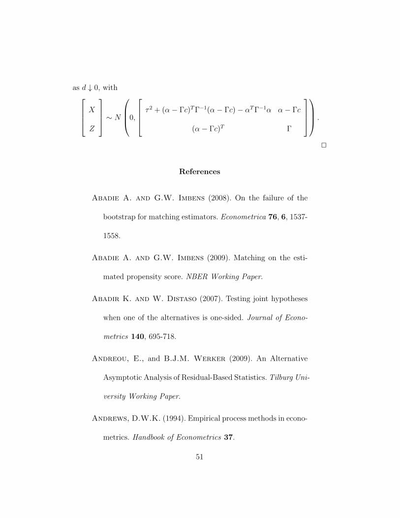
as d ↓ 0, with X

Z

∼ N

0,

τ 2 + (α− Γc)TΓ−1(α− Γc)− αTΓ−1α α− Γc

(α− Γc)T Γ

.

2

References

Abadie A. and G.W. Imbens (2008). On the failure of the

bootstrap for matching estimators. Econometrica 76, 6, 1537-

1558.

Abadie A. and G.W. Imbens (2009). Matching on the esti-

mated propensity score. NBER Working Paper.

Abadir K. and W. Distaso (2007). Testing joint hypotheses

when one of the alternatives is one-sided. Journal of Econo-

metrics 140, 695-718.

Andreou, E., and B.J.M. Werker (2009). An Alternative

Asymptotic Analysis of Residual-Based Statistics. Tilburg Uni-

versity Working Paper.

Andrews, D.W.K. (1994). Empirical process methods in econo-

metrics. Handbook of Econometrics 37.

51

Bai, J., and S. Ng (2001). A consistent test for symmetry in

times series models. Journal of Econometrics 103, 225–158.

Bera, A.K., and G. Premaratne (2005). A test for symmetry

with leptokurtic financial data. Journal of Financial Econo-

metrics 3, 169–187.

Bera, A.K., and G. Premaratne (2009). Adjusting the tests

for skewness and kurtosis for distributional misspecifications.

Working paper.

Bera, A.K., and M.J. Yoon (1993). Specification testing with

misspecified local alternatives. Econometric Theory 9, 649–

658.

Berkes, I., and L. Horvath (2004). The efficiency of the es-

timator of the parameters in GARCH processes. The Annals

of Statistics 32, 633–655.

Bickel, P.J., C.A.J. Klaassen, Y. Ritov, and J.A. Well-

ner (1993). Efficient and Adaptive Statistical Inference for

Semiparametric Models. John Hopkins University Press, Bal-

timore.

52

Cotter, K.D., (1986). Similarity of information and behavior

with a pointwise convergence topology. Journal of Mathemat-

ical Economics 15, 25–38.

Drost, F.C. and C.A.J. Klaassen (1997). Efficient estima-

tion in semiparametric GARCH models. Journal of Econo-

metrics 81, 193–221.

Hallin, M. and M.L. Puri (1991). Time series analysis via

rank-order theory: signed-rank tests for ARMA models. Jour-

nal of Multivariate Analysis 39, 175–237.

Jeganathan, P. (1995). Some aspects of asymptotic theory

with applications to time series models. Econometric The-

ory 11, 818–887.

Le Cam, L. and G.L. Yang (1990). Asymptotics in Statistics;

Some Basic Concepts. Springer, Berlin.

Linton, O. (1993). Adaptive estimation in ARCH models. Econo-

metric Theory 9, 539–569.

Lumsdaine, R. (1996). Consistency and asymptotic normality of

the quasi-maximum likelihood estimator in IGARCH(1,1) and

53

covariance stationary GARCH(1,1) models. Econometrica 64,

575–596.

Murphy, K., and R. Topel (1985). Estimation and inference

in two-step econometric models. Journal of Business and Eco-

nomic Statistics 3, 370–379.

Murphy, K., and R. Topel (2002). Estimation and inference

in two-step econometric models. Journal of Business and Eco-

nomic Statistics 20, 88–97.

Nelson, D. (1990). Stationarity and persistence in the GARCH(1,1)

model. Econometric Theory 6, 318–334.

Newey, W., and D. McFadden (1994). Large sample esti-

mation and hypothesis testing. Handbook of Econometrics,

Ch. 36, Vol. IV, R. Engle and D. McFadden (eds.).

Pagan, A. (1986). Two Stage and Related Estimators and Their

Applications. The Review of Economic Studies 53, 517–538.

Pagan, A., and F. Vella (1989). Diagnostic tests for mod-

els based on individual data: A Survey. Journal of Applied

Econometrics 4, S29–S59.

54

Pierce, D.A. (1982). The asymptotic effect of substituting esti-

mators for parameters in certain types of statistics. The An-

nals of Statistics 10, 475–478.

Ploberger, W. (2004). A complete class of tests when the like-

lihood is locally asymptotically quadratic. Journal of Econo-

metrics, 118, 67-94

Pollard, D. (1989). Asymptotics via empirical processes, Sta-

tistical Science 4, 341–366.

Randles, R.H. (1982). On the asymptotic normality of statistics

with estimated parameters. The Annals of Statistics 10, 462–

474.

Strasser, H. (1985). Mathematical Theory of Statistics. Walter

de Gruyter, New York.

Sun, Y., and T. Tsengos (2006). Semiparametric efficient adap-

tive estimation of asymmetric GARCH models. Journal of

Econometrics 133, 373–386.

van der Vaart, A. (1998). Asymptotic Statistics. Cambridge

University Press, Cambridge.

55