ClickHere

for

FullArticle

An almost‐free barotropic mode in the Australian‐Antarctic Basin

Wilbert Weijer1

Received 25 January 2010; revised 19 April 2010; accepted 20 April 2010; published 19 May 2010.

[1] The Australian‐Antarctic Basin (AAB) is known forits high levels of intraseasonal variability; sea‐surfaceheight variability exceeds background values by factors of2 over thousands of kilometers. This paper addresses thehypothesis that this variability is caused by trapping ofbarotropic energy by the basin geometry. Analysis of amulti‐year integration of a shallow‐water model shows thatthe variability is dominated by a single, large‐scalestatistical mode that is highly coherent over the entire AAB.The flow associated with this mode is northwestward alongthe Southeast Indian Ridge, southward in the KerguelenAbyssal Plain, and eastward in the southern AAB. Themode is interpreted as an almost‐free topographicallytrapped mode, as it is confined by contours of potentialvorticity that almost entirely enclose the AAB. The apex ofthe Wilkes Abyssal Plain represents the strongest barrier tothe modal circulation: here velocities are strongest, makingit a key area for dissipation of kinetic energy throughbottom friction and eddy viscosity. Citation: Weijer, W.(2010), An almost‐free barotropic mode in the Australian‐AntarcticBasin , Geophys . Res . Le t t . , 37 , L10602, doi :10 .1029/2010GL042657.

1. Introduction

[2] Wind forcing is among the main drivers of the oceancirculation. It is believed to be an important source of energyfor turbulence‐driven mixing in the abyss and, as such,essential for maintaining a vigorous overturning circulation[e.g.,Wunsch and Ferrari, 2004]. Identifying how and wherethis energy is dissipated is thus important for understandingthe dynamics of the global‐scale ocean circulation and its rolein climate.[3] The Southern Ocean has been identified as an impor-

tant region for the energetics of the global circulation [e.g.,Wunsch, 1998]. Here, the vigorous wind forcing and weakstratification allow for an energetic circulation that is stronglycontrolled by bathymetry. In fact, analysis of altimeter datahave identified several regions in the Southern Ocean wheresea‐surface height (SSH) variability is exceptionally strong[e.g.,Chao and Fu, 1995]. One of these areas is the Australian‐Antarctic Basin (AAB, Figure 1). Located between AustraliaandAntarctica, it accommodates the Kerguelen Abyssal Plain(KAP) and the Wilkes Abyssal Plain (WAP), as well as anextensive mid‐ocean ridge system known as the SoutheastIndian Ridge (SIR). This ridge consists of eastern (ESIR) andwestern (WSIR) segments that are offset by the WAP.[4] Studies addressing the anomalous SSH variability in

the AAB suggest a link with the local bathymetry [e.g., Chao

and Fu, 1995; Fukumori et al., 1998; Ponte and Gaspar,1999; Webb and De Cuevas, 2002; Fu, 2003; Vivier et al.,2005; Weijer and Gille, 2005a; Weijer et al., 2009]. In par-ticular, Webb and De Cuevas [2002] (hereafter WD02) con-cluded that the enhanced variability reflects the resonantexcitation of a topographically trapped mode. However, theyfound this mode to decay too fast to be consistent with fric-tional spin‐down [e.g.,Fu, 2003;Weijer et al., 2009]. Instead,they suggested that energy may be leaking from the mode atthe apex (‘mouth’) of theWAP, and escape along the northernflank of the WSIR. This conclusion was supported by Vivieret al. [2005], who found that SSH variability in the AABincreased in their model when they turned off the inertia term,apparently at the expense of the variability on the WSIR.[5] Weijer et al. [2009] (hereafter WGV) have shown that

at least part of the SSH variability can indeed be attributedto the resonant excitation of free topographically trappedmodes. These modes represent balanced circulation patternsalong closed contours of potential vorticity (defined as f /H,where f is the Coriolis parameter andH the local water depth)that surround in particular the WAP and the crest of theWSIR. However, the two dominant modes were found toexplain only a fraction of the variance, leaving the maincharacteristics of the anomalous SSH variability unaccountedfor. In addition, the slow, frictional decay of these modes isinconsistent with the rapid decay found by WD02.[6] In this paper we study the dynamics of the variability

in the AAB that was unexplained by WGV. The analysissuggests that the specific distribution of f /H in the AABgives rise to a so‐called almost‐free mode response to windstress forcing [Hughes et al., 1999]. This response is char-acterized by i) highly coherent motion over the entire AAB;ii) flow aligned mostly along contours of f /H surroundingthe basin; iii) a key region where the flow has to jump con-tours of f /H; leading to iv) relatively rapid decay comparedwith the frictional spin‐down of purely free modes. A detailedanalysis of the energetics shows that the modal response is avery important aspect of the regional circulation as it funnelsenergy towards the apex of the WAP for dissipation, and fortransfer to non‐modal flow.

2. Method

[7] Since the anomalous variability in the AAB is thoughtto be dominantly barotropic, a 1‐layer shallow‐water (SW)model is used to study its most important characteristics. Thecomputational domain ranges from 45° to 185° east longi-tude, and from −70° to 0° latitude, encompassing the SouthIndian Ocean and the Indian sector of the Southern Ocean.Diagnostic focus is on a subdomain that ranges from 68° to145° east longitude and −65° to −30° latitude, covering thegreater AAB. Forcing is provided by daily‐averaged windstress, based on the 10mwind velocity ofMilliff et al. [2004].The model was integrated for 1003 days, starting August 1,

1Los Alamos National Laboratory, Los Alamos, New Mexico, USA.

Copyright 2010 by the American Geophysical Union.0094‐8276/10/2010GL042657

GEOPHYSICAL RESEARCH LETTERS, VOL. 37, L10602, doi:10.1029/2010GL042657, 2010

L10602 1 of 4

1999, and daily averages of the dynamical fields h, u andv (SSH, and the zonal and meridional velocity components,respectively) were saved. In order to focus on the variabilitythat could not be explained by free modes, we repeated thenormal‐mode analysis of WGV to determine as many modesas possible, and filtered out their signal from the dynamicalfields. Subsequent analyses described below are based onthese residual fields. In some areas, specifically the WAP,the free modes account for up to 50% of the SSH variability.See section 1 of the auxiliary material for a more detaileddescription of the modeling approach.1

3. A Topographically Trapped Mode in the AAB

3.1. Spatial Structure

[8] In order to determine the spatial structure of the vari-ability we first perform an Empirical Orthogonal Function(EOF) analysis on the daily‐averaged SSH fields, box‐averaged onto a coarser grid of 2° × 2° resolution. The analysisis dominated by the first EOF, which accounts for 46.6% ofthe SSH variance (section 2.1 of the auxiliary material). Thepattern clearly resembles the dominant EOFs of SSH vari-ability determined by WD02 and Fu [2003]. Additional sta-tistical analyses (section 2.2 of the auxiliary material) showthat the EOF represents variability that is highly coherentthroughout the basin: local SSH time series are significantlycoherent with its amplitude time series (principal component)G1(t) for essentially all frequencies below 1/30 cpd; time lagsare a few days at most.[9] The principal component G1 is used to construct a

composite pattern of the SSH and velocity fields that we willrefer to as the statistical mode: um = u�1, where u = (u, v, h),and the overline denotes the average over the 1003‐day timeseries (Figure 2). The composite pattern of SSH is equivalentto the EOF except for the higher spatial resolution; it showspositive loadings in the entire AAB. In fact, the pattern is

clearly enclosed by the blue and red contours of potentialvorticity (representing values of −3.2 · 10−8 and −2.5 ·10−8m−1 s−1, respectively), that nearly bound the basin. Thecirculation associated with this pattern displays intense north-westward transport along the northern flank of the WSIRand the southern flank of the ESIR; broad southward flows inthe basin between the WSIR and the Kerguelen Plateau; andeastward drifts in the southern part of the basin.[10] In summary, almost half of the variability in the AAB

is captured by a single EOF. The facts that the associatedvariability is i) stationary and highly coherent, and ii) stronglylinked to bathymetry, support the interpretation that it is causedby a topographically trapped mode. In the remainder of thispaper we assume that the statistical mode represents such adynamical object.

3.2. Decay and Energetics

[11] To study the decay of the topographically trappedmode, we use the velocity field of the statistical modedepicted in Figure 2 to initialize a transient, unforced inte-gration of the SW model. The model is run for 10 days.Projection of the composite velocity patterns on the dailyaveraged velocity fields yields the two projection time seriesgu and gv for zonal and meridional velocity, respectively.These time series record a rapid decay, and reach the 1/ethreshold after about 5 or 6 days (section 3 of the auxiliarymaterial). This decay rate is much faster than what can beexpected from frictional spin‐down. In fact, similar rapiddecay was deduced by WD02, who suggested that the modemay lose energy to non‐modal circulation.[12] In order to address this hypothesis, we study the

energetics of the mode in the forced and unforced simula-tions. We decompose the velocity field in the modal contri-bution um and a residual ur = u − um at each time step. Based

Figure 1. Bathymetry of the Australian‐Antarctic Basin.ESIR and WSIR: Eastern and western segments of theSoutheast Indian Ridge; WAP: Wilkes Abyssal Plain; KAP:Kerguelen Abyssal Plain. Black contours are isolines of thebase‐10 logarithm of f /H (scaled by −1 m−1 s−1), plotted forthe interval [−9.0, −7.0] with step 0.5.

Figure 2. Composite fields of SSH (shading; in meters) andvelocity (arrows), obtained by regressing the daily‐averagedfields on G1. Velocity vectors denote box‐averaged valuesover squares of 5 × 5 grid points. Maximum values areof the order of 0.02 m s−1. Contours represent isolines off /H as in Figure 1; blue, yellow and red contours representthe values −3.2 × 10−8, −2.8 × 10−8 and −2.5 × 10−8 m s−1,respectively.

1Auxiliary materials are available in the HTML. doi:10.1029/2010GL042657.

WEIJER: AUSTRALIAN-ANTARCTIC BASIN L10602L10602

2 of 4

on this decomposition, we can determine a balance for thekinetic energy of the actual mode, Em = 1

2r0H∣um∣2, and of

the residual, Er = 12r0H∣ur∣

2:

dEm

dt¼ Fm þ Rm þWm ð1aÞ

dEr

dt¼ Fr þ Rr þWr ð1bÞ

Input of kinetic energy by wind stress forcing is indicatedby W, local dissipation due to friction by R, while the resid-ual F represents other mechanisms of energy transfer. Thesemechanisms include work done by the Coriolis and pressuregradient forces that either transfer energy between Em andEr, or remove energy locally to be deposited elsewhere. Seesection 4 of the auxiliary material for a detailed discussion ofthese terms.[13] Figure 3 shows the terms in the kinetic energy balance

equations (1a) and (1b), averaged over the first 6 days of theunforced, decaying integration. Energy input bywind stress iszero. Terms in brackets denote the values integrated over themodal area, defined as the region where the amplitude of thedominant EOF exceeds 1/6th of its maximum value (indi-cated by the yellow contour in the top plots).[14] The area‐integrated values show that the mode loses

25% (1.79 GW) of its energy locally to frictional processes.This energy loss is concentrated at the apex of the WAP.About 17% (1.22 GW) is exported from the modal area

altogether by energy fluxes. The largest part (57%; 4.04 GW),however, is transferred to the residual circulation within themodal area. Although the mode loses most of its energy overthe northern flank of the WSIR and along the northwesternedge of the WAP, the residual circulation picks up most of itsenergy at the apex of theWAP. A flux of energy is implied bythese sources and sinks, and evidently the apex of theWAP isan area of energy flux convergence. A substantial part of theenergy gained by the residual circulation is immediatelydissipated by friction.[15] Analysis of the energetics of the 1003‐day forced run

is fully consistent with this picture (Figure 4). No less than21% (0.37 GW, the average over the 1003 days of integra-tion) of the energy input by the wind stress is used to energizethe mode. About 38% of this energy (0.14 GW) is dissipatedthrough friction, most of which at the apex of the WAP. Aswas the case for the unforced simulation, there is a stronglocalized source of energy for the non‐modal circulation atthe apex of theWAP, and it is likely that a substantial fractionof this energy is derived from the mode. These results suggestthat also in the wind forced case there is a significant transferof energy from the mode to the residual circulation, and thatthe prime location for this transfer is the apex of the WAP.

4. Summary and Discussion

[16] In this paper we studied the nature of the high SSHvariability in the AAB. The analysis suggests that the vari-ability identified byWD02 and Fu [2003] is indeed caused bythe resonant excitation of a topograpically trapped mode. Itis found that similar variability i) can be reproduced by abarotropic SW model forced with realistic wind stress; ii) is

Figure 3. Terms in the balance of kinetic energyequations (1a) and (1b) for the unforced, decaying integra-tion (in mW m−2). Numbers in brackets denote integrals (inGW) over the modal area. This area is indicated by the yellowline in the top left plot. Work done by wind stress is zero. Seetext for details.

Figure 4. As Figure 3, but now for the forced integration.The tendency terms are negligibly small, and incorporated inF for completeness. Top plots now show work done by windstress.

WEIJER: AUSTRALIAN-ANTARCTIC BASIN L10602L10602

3 of 4

clearly confined by specific contours of potential vorticitythat almost completely enclose the AAB; and iii) has a highspatial coherence for all time scales exceeding a month, dis-playing a negligible time lag of ±2 days over the extent of thebasin.[17] What is the nature of this mode? Despite a large

number of normal‐mode calculations, WGV found no freemodes that are consistent with the statistical mode determinedin this study. Although it is impossible to determine allmodes, the analysis usually determines the ‘strongest’modeswith ease, and it seems unlikely that the current mode wassimply missed.[18] A more likely interpretation is that the statistical mode

does not reflect a free mode in the strictest sense of the word:a dynamical object that fully preserves its spatial structurewhile evolving in time. Instead, it shows characteristics of analmost‐free mode, a concept introduced by Hughes et al.[1999] to explain a band of high SSH variability aroundAntarctica called the Southern Mode. As is the case there, theAAB is surrounded by contours of f /H that are almost con-tinuous, if not for a few choke points, most notably the apexof the WAP. Hughes et al. [1999] argued that a continuouscirculation can only exist by the grace of a vorticity sourceat the choke points that allows the flow to jump contours off /H. In the absence of forcing (and significant friction), themode can only negotiate the jump in f /H by a local change inrelative vorticity, causing the mode to lose its coherence andhence its true modal character. Indeed, in the decaying sim-ulation the advection of potential vorticity attains its maxi-mum amplitudes there (not shown). And although frictiondoes its part, there is a substantial residual that locally gen-erates relative vorticity.[19] It is clear from this study that the topographically

trapped mode has significant impact on the energetics of theAAB. It receives a substantial amount of energy from thewind, but instead of expending it on friction (as would bethe case for the free modes described in WGV), most ofthe energy is funneled to the apex of the WAP to powera residual, non‐modal circulation. This result supports theconclusion byWD02 and Vivier et al. [2005], who suggestedthat energy may be extracted from the mode by waves ema-nating from the apex of the WAP, and propagating alongthe northern flank of the WSIR. The mode plays hence animportant role in redistributing energy over large distances[e.g., Weijer and Gille, 2005b], and points to the apex of

the WAP as a potential location of enhanced dissipativemixing.

[20] Acknowledgments. This research was supported by the ClimateChange Prediction Program of the U.S. Department of Energy Office ofScience and by NSF‐OCE award 0928473. Los Alamos National Laboratoryis operated by the Los Alamos National Security, LLC for the NationalNuclear Security Administration of the U.S. Department of Energy undercontract DE‐AC52‐06NA25396. Wind stress curl data were provided bythe Data Support Section of the Computational and Information SystemsLaboratory at the National Center for Atmospheric Research. Constructivecomments by Matthew Hecht and two anonymous reviewers are gratefullyacknowledged.

ReferencesChao, Y., and L.‐L. Fu (1995), A comparison between the TOPEX/

POSEIDEON data and a global ocean general circulation model during1992–1993, J. Geophys. Res., 100, 24,965–24,976.

Fu, L.‐L. (2003), Wind‐forced intraseasonal sea level variability of theextratropical oceans, J. Phys. Oceanogr., 33, 436–449.

Fukumori, I., R. Raghunath, and L.‐L. Fu (1998), Nature of global large‐scale sea level variability in relation to atmospheric forcing: A modelingstudy, J. Geophys. Res., 103, 5493–5512.

Hughes, C. W., M. P. Meredith, and K. J. Heywood (1999), Wind‐driventransport fluctuations through Drake Passage: A southern mode, J. Phys.Oceanogr., 29, 1971–1992.

Milliff, R. F., J. Morzel, D. B. Chelton, and M. H. Freilich (2004), Windstress curl and wind stress divergence biases from rain effects on QSCATsurface wind retrievals, J. Atmos. Oceanic Technol., 21, 1216–1231.

Ponte, R. M., and P. Gaspar (1999), Regional analysis of the invertedbarometer effect over the global ocean using TOPEX/POSEIDON dataand model results, J. Geophys. Res., 104, 15,587–15,601.

Vivier, F., K. A. Kelly, and M. Harismendy (2005), Causes of large‐scale sealevel variations in the SouthernOcean:Analyses of sea level and a barotropicmodel, J. Geophys. Res., 110, C09014, doi:10.1029/2004JC002773.

Webb, D. J., and B. A. De Cuevas (2002), An ocean resonance in theIndian sector of the Southern Ocean, Geophys. Res. Lett., 29(14),1664, doi:10.1029/2002GL015270.

Weijer, W., and S. T. Gille (2005a), Adjustment of the Southern Ocean towind forcing on synoptic time scales, J. Phys. Oceanogr., 35, 2076–2089.

Weijer, W., and S. T. Gille (2005b), Energetics of wind‐driven barotropicvariability in the Southern Ocean, J. Mar. Res., 63, 1101–1125.

Weijer, W., S. T. Gille, and F. Vivier (2009), Modal decay in the Australia‐Antarctic Basin, J. Phys. Oceanogr., 39, 2893–2909.

Wunsch, C. (1998), The work done by the wind on the oceanic general cir-culation, J. Phys. Oceanogr., 28, 2332–2340.

Wunsch, C., and R. Ferrari (2004), Vertical mixing, energy, and the generalcirculation of the oceans, Ann. Rev. Fluid Mech., 36, 281–314.

W. Weijer, CCS‐2, MS B296, Los Alamos National Laboratory, LosAlamos, NM 87545, USA. (wilbert@lanl.gov)

WEIJER: AUSTRALIAN-ANTARCTIC BASIN L10602L10602

4 of 4

Supplemental information to “An almost-free barotropic

mode in the Australian-Antarctic Basin”

Wilbert Weijer ∗

Los Alamos National Laboratory, Los Alamos, New Mexico

April 14, 2010

∗Corresponding author address: Dr. Wilbert Weijer, Los Alamos National Laboratory, NM 87545. E-mail:

wilbert@lanl.gov

1

1 Modeling Approach

1.1 Basic Configuration

To study the variability in the Australian-Antarctic Basin (AAB), we analyze the circulationin a 1-layer shallow-water (SW) model. The model is based on the code by Schmeits andDijkstra (2000), and used by Weijer et al. (2009) (hereafter WGV) to study modal variabilityin the AAB. The results of two integrations are discussed in this paper, a run forced withrealistic wind stress, and an unforced run, initialized with the statistical mode (see below).

The model domain ranges from 45◦ to 185◦ east longitude, and from -70◦ to 0◦ latitude.The numerical grid consists of 210 × 210 grid points, yielding a spatial resolution of 2/3◦ ×1/3◦. Bathymetry is based on the global 2-minute data set ETOPO-2, box-averaged ontoour model grid, and smoothed by applying a 5-point filter to remove the smallest lengthscales. Depths smaller than 300 m (the continental shelf) are set to zero.

Horizontal eddy viscosity is parameterized through a Laplacian formulation with coef-ficient Ah = 3 · 103 m2 s−1, while bottom friction is represented through a linear drag withcoefficient r = 2 · 10−7 s−1. Non-linear advection terms are ignored.

The model was integrated using a Crank-Nicolson scheme with a 15-minute time step.Daily averages of the dynamical fields η, u and v (surface elevation, and the zonal andmeridional velocity components, respectively) were saved. Analysis was performed on a sub-domain that ranges from 68◦ to 145◦ east longitude and -65◦ to -30◦ latitude, encompassingthe greater AAB.

1.2 The forced run

The forced run was integrated for 1003 days, starting August 1, 1999. Forcing was derivedfrom the 10 m wind velocity of Milliff et al. (2004), which consists of QuickSCAT scatterom-eter data blended with NCEP reanalysis. The data, provided at 6-hourly intervals on a 0.5◦

grid, was converted to wind stress according to the drag law of Large and Yeager (2004),interpolated onto our model grid, averaged to daily values, filtered to remove the annual andsemi-annual cycles, and detrended.

WGV showed that a part of the variability was caused by a few normal modes that theywere able to determine using a normal-mode analysis. However, the modes considered inthat study only explained a small fraction of the variance, and the basin-wide pattern ofvariability remained unexplained. In order to focus on this dominant mode of variability, weused the projection method used by Weijer et al. (2007) to remove the contributions of asmany modes as we were able to determine from the dynamical fields.

First, we repeated our normal-mode analysis and identified 6 stationary (real) modes withsignificant expression in the AAB (4 of which were discussed in WGV) and 31 oscillatory(complex) modes. Assuming that the data S(x, t) consists of a superposition of the modesand noise Z (the latter containing the signal that is the subject of this study), we can write:

S(x, t) =M

i=1

ψi(x)γi(t) + Z(x, t) (1)

2

where M is the number of modal patterns ψi and associated time series γi. Multiplying thisequation by each of the modes ψj and integrating over the domain D yields:

DψjS dx dy =

M

i=1

Cjiγi +D

ψjZ dx dy (2)

with:Cji =

Dψjψi dx dy. (3)

The last integral in Eq. (2) vanishes if the noise is spatially uncorrelated to the eigenmodes.The matrix C gives the correlations between the eigenmodes; if the set were orthonormal,C would diagonal, but in general it is not. Therefore, a full matrix inversion was performedto find the unique set of 68 time series γi(t).

As shown by WGV, the projection time series based on η may not always be an accuratemeasure of the modal amplitude. Therefore, the projection was applied to the two velocitycomponents only, and the modal amplitudes γi were estimated by 1

2(γu

i + γvi ), where γu

i andγv

i are the projection time series based on zonal and meridional velocity, respectively.The resulting modal reconstructions were subsequently subtracted from the three model

fields. As in WGV, the modal contributions explain only a small part of the overall SSHvariability. The reconstruction is most successful in the WAP, where free modes account forabout 50% of SSH variability (Fig. 1).

1.3 The unforced run

In addition to the forced run, we performed an unforced simulation that was initialized by thestatistical mode. As described in the main paper, this mode was constructed by regressingthe dominant principal component of SSH variability (see below) onto the three model fields.The simulation was run for 10 days.

Only the velocity fields were used to initialize the model. Initializing SSH as well wouldhave resulted in vigorous gravity wave activity, as the fields of the statistical mode arenot in exact geostrophic balance. Instead, initializing with only the velocity field almostimmediately sets up the SSH field that brings the flow in geostrophic balance.

2 Statistical Analysis

2.1 EOF analysis

The character of the SSH variability in the AAB is analyzed by performing an EmpiricalOrthogonal Function (EOF) analysis on the daily-averaged SSH fields, filtered to removethe free modes, and box-averaged onto a coarser grid of 2◦ × 2◦ resolution. The analysisis dominated by the first EOF, which captures 46.6% of the SSH variance in the area onthis coarser grid (Fig. 2). Its spatial pattern is almost indistinguishable from the dominantEOF of the original data set, where it explained 43.4% of the variability. This indicates thatthe free modes removed from the data do not contribute to the leading (statistical) mode ofvariability of the system. It also clearly resembles the dominant EOFs of SSH variability inthe area as presented by Fu (2003) and Webb and De Cuevas (2002).

3

latitude

70 80 90 100 110 120 130 140

−60

−50

−40

−30

0

0.02

0.04

0.06

latitude

70 80 90 100 110 120 130 140

−60

−50

−40

−30

0

0.02

0.04

0.06

longitude

latitude

70 80 90 100 110 120 130 140

−60

−50

−40

−30

0

0.02

0.04

0.06

Figure 1: Standard deviation of the total SSH field (upper panel), the residual, filtered SSHfield (central panel), and the combined effect of the 68 modal contributions (lower panel).

2.2 Spatial coherence

In order to determine to what extent the dominant EOF represents variability that is spatiallycoherent, we studied the statistical relationship between local SSH variations and the firstPrincipal Component Γ1 (the time series of the dominant EOF; Fig. 3). First, a correlationanalysis was performed for lags between ±12 days. The maximum correlation (or anti-correlation, whichever is stronger) is plotted in Fig. 3a, while panel b shows the lag for whichthe maximum (anti-)correlation occurs. It is clear that Γ1 is strongly (and significantly)correlated with basically all SSH time series in the domain, but most strongly so in the areaof anomalous SSH variability indicated by the dominant EOF. Here correlations up to 0.9are found. Also, in this area the time lag is typically within ±2 days: SSH slightly leads Γ1

in the KAP, and lags on the norhern flank of the SIR and in the WAP.A coherence analysis between Γ1 and local SSH gives a complementary view of the spatial

4

longitude

latitude

70 80 90 100 110 120 130 140

−65

−60

−55

−50

−45

−40

−35

−0.05

−0.04

−0.03

−0.02

−0.01

0

0.01

0.02

0.03

0.04

0.05

Figure 2: Dominant EOF of the variability in the AAB. Black contours are isolines ofthe base-10 logarithm of f/H, plotted for the interval [−9.0,−7.0] with step 0.5. Blue,yellow and red contours highlight the isolines with f/H values −3.2 · 10−8, −2.8 · 10−8 and−2.5 · 10−8m−1 s−1, respectively.

coherence of the variability. The analysis generally shows a strong and significant coherencebetween the time series for all frequencies upto a certain threshold, beyond which the coher-ence rather abruptly breaks down. To determine this cut-off frequency fmax, we diagnose thefirst frequency (starting from f = fmin, where fmin = 1/167 cpd is the minimum frequencyresolved) at which the time series lose their coherence. Figure 3c shows the associated timescale 1/fmax of this measure. In the area of anomalous SSH variability there is significantcoherence between Γ1 and local SSH time series for a very broad frequency range. For mostof the central basin the time series are coherent at least up to frequencies of 1/30 cpd, witha maximum cut-off frequency of 1/5 cpd in the center. Panel d shows the time lag, averagedover this frequency window of significant coherences. This time lag τ(f) is determined fromthe coherence phase ϕ(f) (in degrees) according to τ = ϕ/360f , with f the frequency. Itdisplays the same pattern as panel b, with SSH showing a slight lead on Γ1 in KAP, and aslight lag in the WAP and on the northern flank of the SIR.

3 Forcing and Decay

A strong relation between modal amplitude and area-integrated wind stress curl was foundby previous studies. Here we use the modal amplitude (as measured by Γ1) to estimatethe wind stress pattern that is related to the mode. Figure 4 shows that there is strongcovariance (and correlation) between Γ1 and wind stress. The strongest co-variation is foundwith wind stress along the periphery of the modal area, oriented mostly parallel to contoursof f/H. Specifically, positive values of Γ1 are correlated with southeasterly winds on the

5

Figure 3: Statistical relationships between local SSH time series and the principal componentΓ1. a) Maximum correlation probed for lags between -12 and 12 days. Basically all correla-tions unequal to zero are statistically significant at the 95% level; b) lag (in days) at whichthis maximum occurs (positive if SSH lags Γ1); c) Inverse of the cut-off frequency 1/fmax (indays) above which the coherence between SSH and Γ1 breaks down for the first time. Coher-ence spectra are smoothed with a 13-point Daniell filter. Black areas (other than continentmasks) indicate regions where the coherence is not significant at fmin; d) the time lag (days)between Γ1 and SSH, averaged over the frequency window [fmin, fmax]. Color scale saturatesat ±12 days.

northern flank of the WSIR, northerly winds over the Kerguelen Plateau and the KAP, andwesterly winds along the Antarctic continental shelf.

The decay of the mode was diagnosed from the unforced, decaying simulation, which wasinitialized by the velocity field of the statistical mode. Projection of the composite velocitypatterns on the daily averaged velocity fields yields two projection time series, γu and γv

(Fig. 5). These time series record a rapid decay, and reach the 1/e threshold after about 5or 6 days.

The projection time series based on the modal sea surface height pattern (γη) shows aneven more rapid decay. As stated before, the empirical pattern of SSH (used as projectionpattern) is unlikely to be in balance with the associated flow field. The SSH field that arisesquickly after initialization with the empirical velocity patterns does therefore not conformperfectly with the empirical SSH pattern that is used here for the projection. Also, as wasthe case for the purely free modes, the modal SSH pattern may project onto noise and maytherefore not be a perfect representation of the modal amplitude.

6

longitude

latitude

70 80 90 100 110 120 130 140

−65

−60

−55

−50

−45

−40

−35

−30

0.1

0.2

0.3

0.4

0.5

0.6

Figure 4: Cross-correlation (shading) and cross-covariance (arrows) between between Γ1 andwind stress τ = (τx, τy), probed for lags between ± 5 days. Cross-correlation is determined as

ρ = (ρ2x + ρ2

y), where ρ(x,y) = ρ(Γ1, τ(x,y)) are the individual (normalized) cross-covariances.

All nonzero correlations are significant. In general, wind stress leads Γ1 by just a few days.

4 Energetics

4.1 Kinetic energy balance

In this section, we analyze the energetics of the modal decay in detail. We start off with aschematic version of the shallow-water (SW) momentum equations used in this study:

∂u

∂t+ fk × u = −g η − ru +

τ

ρ0H. (4)

For convenience of notation, we consider the equations in a Cartesian frame, and neglectthe explicit representation of horizontal viscosity. Here, τ is the wind stress vector, r is thecoefficient of bottom friction, g is the gravitational constant, ρ0 a reference density, and fthe Coriolis parameter.

In order to study the energy loss of the purely modal circulation, we decompose thevelocity field at each time step in a modal component and a residual: u = um + ur. Bymultiplying Eq. (4) by um and ur we obtain two equations describing the energetics of boththe modal and non-modal component:

Tmm = Tmr + Cmm + Cmr + Pm + Rmm + Rmr + Wm (5a)

Trr = Trm + Crr + Crm + Pr + Rrr + Rrm + Wr (5b)

7

0 2 4 6 8 100

0.1

0.2

0.3

0.4

0.5

0.6

0.7

0.8

0.9

1

Time (days)

γuγvγη

exp(−t/7)

Figure 5: Daily-averaged projection time series for the zonal and meridional velocity compo-nents, and for sea-surface height, for the 10 days of the unforced, decaying simulation.

where:Tmm = 1

2ρ0H

∂∂t|um|

2 Trr = 12ρ0H

∂∂t|ur|

2

Tmr = −ρ0Hum · ∂∂t

ur Trm = −ρ0Hur ·∂∂t

um

Cmm = −ρ0Hfum · k × um Crr = −ρ0Hfur · k × ur

Cmr = −ρ0Hfum · k × ur Crm = −ρ0Hfur · k × um

Pm = −ρ0gHum · η Pr = −ρ0gHur · ηRmm = −ρ0Hr|um|

2 Rrr = −ρ0Hr|ur|2

Rmr = −ρ0Hrum · ur Rrm = −ρ0Hrur · um

Wm = um · τ Wr = ur · τ

The terms T denote tendency terms of modal kinetic energy Emm = 12ρ0H|um|

2, theresidual kinetic energy Err = 1

2ρ0H|ur|

2, and a mixed-mode kinetic energy Emr = ρ0Hum·ur.Terms labeled C, P , R and W represent work done by the Coriolis force, the pressuregradient force, friction, and wind stress. In the continuous representation of the system,work done by the Coriolis force should be zero, so that Cmm = Crr = 0 and Cmr = −Crm.In addition, Rmr = Rrm. For a discretized system, these conditions do not necessarily hold.In particular, for a C-grid discretization the Coriolis force does perform work locally, andalthough the global integral vanishes, integration over a subdomain will in general not bezero. For the numerical representation of a purely geostrophic flow, the sum of work done bythe pressure gradient and the coriolis force should add up to zero, so that C + P reflects thecombined work of the Coriolis and pressure gradient forces on the ageostrophic component.In practice, C can be considered as the divergence of a short-range, non-physical energy flux.

8

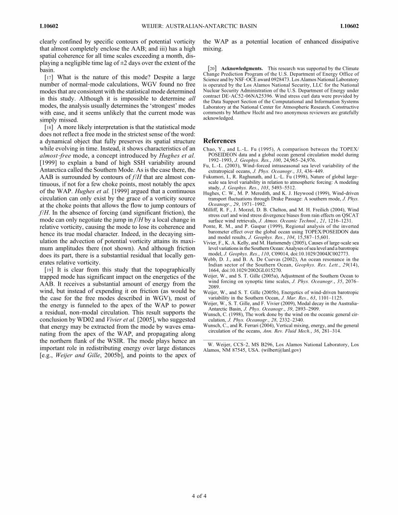
Tmm = -7.33 Trr = 2.83 Tmm + Trr = -4.23Tmr = -0.25 Trm = 0.31 Tmr + Trm = -0.06Cmm = -0.33 Crr = -0.16 Cmm + Crr = -0.48Cmr = -1.69 Crm = 1.38 Cmr + Crm = -0.48Pm = -3.00 Pr = 2.51 Pm + Pr = -0.49Rmm = -1.52 Rrr = -0.97 Rmm + Rrr = -2.49Rmr = -0.27 Rrm = -0.25 Rmr + Rrm = -0.52

Table 1: Terms in the kinetic energy equations (in GW) for the unforced, decaying simulation.Terms are averaged over the first 6 days of integration, and integrated over the domainindicated by the yellow line in Fig. 6.

4.2 Energy transfers for the unforced run

We diagnosed the individual terms in Eq. (5) for the 10-day unforced integration, initializedwith the composite velocity field um. The kinetic energy of the residual flow Err peaks atday 6, so the terms are averaged over the first 6 days of integration. The spatial distributionsare plotted in Fig. 6, a condensed version of this plot is presented as Fig. 3 of the mainmanuscript. The values integrated over the modal area (defined as the area where theamplitude of η exceeds 20% of the maximum, indicated by the yellow line in Fig. 6) arelisted in Table 1. Since the integration is unforced, wind work W is zero.

It is clear that a substantial transfer of kinetic energy takes place from the mode tothe residual, non-modal circulation. Several terms take part in this exchange, in particularthe Coriolis exchange terms (Cmr ≈ −Crm), the pressure work terms (Pm and Pr), and thetendency of the mixed-mode kinetic energy (Tmr ≈ −Trm). Note that the actual work doneby the Coriolis force (Cmm and Crr) is among the smallest terms in the individual columns,although the total work done by the Coriolis force is of same order of magnitude as the totalwork done by pressure. Also Rmr ≈ Rrm, as could be expected.

In the main paper, the following notation convention is used:

main paper supplemental informationEm Emm

Fm Tmr + Cmm + Cmr + Pm

Rm Rmm + Rmr

Wm Wm

Er Err

Fr Trm + Crr + Crm + Pr

Rr Rrr + Rrm

Wr Wr

(6)

References

Fu, L.-L., 2003: Wind-forced intraseasonal sea level variability of the extratropical oceans.J. Phys. Oceanogr., 33, 436–449.

9

Large, W. G. and S. Yeager, 2004: Diurnal to decadal global forcing for ocean and sea-icemodels: the data sets and flux climatologies. Tech. rep., National Center for AtmosphericResearch, Boulder, CO, U.S.A.

Milliff, R. F., J. Morzel, D. B. Chelton, and M. H. Freilich, 2004: Wind stress curl and windstress divergence biases from rain effects on QSCAT surface wind retrievals. J. Atmos.Ocean. Tech., 21, 1216–1231.

Schmeits, M. J. and H. A. Dijkstra, 2000: Physics of the 9-month variability in the GulfStream region: combining data and dynamical systems analysis. J. Phys. Oceanogr., 30,1967–1987.

Webb, D. J. and B. A. De Cuevas, 2002: An ocean resonance in the Indian sector of theSouthern Ocean. Geophys. Res. Letters, 29(14), 10.1029/2002GL015 270.

Weijer, W., S. T. Gille, and F. Vivier, 2009: Modal decay in the Australia-Antarctic Basin.J. Phys. Oceanogr., 39, 2893–2909.

Weijer, W., F. Vivier, S. T. Gille, and H. Dijkstra, 2007: Multiple Oscillatory Modes of theArgentine Basin. Part I: Statistical analysis. J. Phys. Oceanogr., 37, 2855–2868.

10

latitude

Tmm (−7.06)

−60

−40

Trr (2.83) Tmm+Trr (−4.23)

latitude

Tmr (−0.25)

−60

−40

Trm (0.31) Tmr+Trm (−0.06)

latitude

Cmm (−0.33)

−60

−40

Crr (−0.16) Cmm+Crr (−0.48)

latitude

Cmr (−1.69)

−60

−40

Crm (1.38) Cmr+Crm (−0.48)

latitude

Pm (−3.00)

−60

−40

Pr (2.51) Pm+Pr (−0.49)

latitude

Rmm (−1.52)

−60

−40

Rrr (−0.97) Rmm+Rrr (−2.49)

latitude

Rmr (−0.27)

longitude80 100 120 140

−60

−40

Rrm (−0.25)

longitude80 100 120 140

Rmr+Rrm (−0.52)

longitude80 100 120 140

−0.01

0

0.01

−0.01

0

0.01

−0.01

0

0.01

−0.01

0

0.01

−0.1

0

0.1

−0.1

0

0.1

−0.01

0

0.01

Figure 6: Terms in the balance of kinetic energy for the unforced, freely decaying run. Termsare averaged over the first 6 days of integration. Color scales from −cmax (blue) to cmax

(red). cmax = 0.014W for all plots except those of Cmr etc. and P , where cmax = 0.15W.Integral values (in GW) are shown in brackets and correspond to those listed in Table 1.Yellow line denotes the area for which integrals were determined.

11