An Algorithm for Multi-Axis Autonomous Rendezvous and Docking

David B Mittelman

NASA Flight Robotics Lab, Marshall Space Flight Center

Drive Actuator selection for autonomous operation, especially in space applications, has been restricted to the manipulation of only two degrees of freedom at a time. With the development of an algorithm to modify all the degrees of freedom at the same time, the

time to target and resource consumption could be reduced.

I. Introduction Automated operations in space have been traditionally avoided in favor of human controlled maneuvers.

However, autonomous control has many advantages if executed properly. There are three major tasks that human controller do without through practice that a control program will have to execute: Flight path planning, signal processing, and decision-making.

II. Algorithms a) Flight Planning

Getting from point A to point B in Space intuitively seems simple. However, there are many considerations that have to be taken into account when doing so. Momentum becomes a large problem considering a frictionless environment. In addition, getting to point B doesn’t do any good if you aren’t facing in the right direction, or aren’t lined up properly for docking. Choosing a proper flight path is critical in this situation. Luckily, there are some mathematical functions that generate a flight path that has many advantages in terms of autonomously docking.

The function utilized in this implementation is the Logistic Function, seen in Figure 1. The red plot on the left shows the fundamental logistic function. However, this function does not allow stabilization at the end of the function. The ideal change would be quick, with a long lead-time and trail time. In addition, the function should start changing after it’s zero point. Equations 1 & 2 show the fundamental logistic function as well as the modified function used for a proper path.

𝑃 𝑡 =1

1+ 𝑒!!   Equation 1: Logistic Function

𝑃 𝑡 =1

1+ 𝑒!!!! !!

 

Equation 2: Logistic Function

Figure 1: Logistical Functions

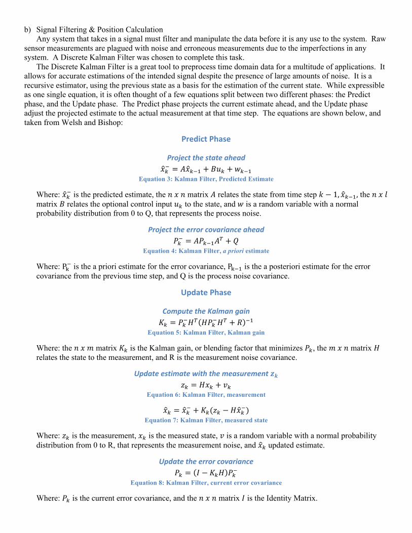
b) Signal Filtering & Position Calculation Any system that takes in a signal must filter and manipulate the data before it is any use to the system. Raw

sensor measurements are plagued with noise and erroneous measurements due to the imperfections in any system. A Discrete Kalman Filter was chosen to complete this task.

The Discrete Kalman Filter is a great tool to preprocess time domain data for a multitude of applications. It allows for accurate estimations of the intended signal despite the presence of large amounts of noise. It is a recursive estimator, using the previous state as a basis for the estimation of the current state. While expressible as one single equation, it is often thought of a few equations split between two different phases: the Predict phase, and the Update phase. The Predict phase projects the current estimate ahead, and the Update phase adjust the projected estimate to the actual measurement at that time step. The equations are shown below, and taken from Welsh and Bishop:

Predict  Phase  

Project  the  state  ahead  𝑥!! = 𝐴𝑥!!! + 𝐵𝑢! + 𝑤!!!

Equation 3: Kalman Filter, Predicted Estimate

Where: 𝑥!! is the predicted estimate, the 𝑛  𝑥  𝑛 matrix 𝐴 relates the state from time step 𝑘 − 1, 𝑥!!!, the 𝑛  𝑥  𝑙 matrix 𝐵 relates the optional control input 𝑢! to the state, and 𝑤 is a random variable with a normal probability distribution from 0 to Q, that represents the process noise.

Project  the  error  covariance  ahead  𝑃!! = 𝐴𝑃!!!𝐴! + 𝑄

Equation 4: Kalman Filter, a priori estimate

Where: P!! is the a priori estimate for the error covariance, P!!! is the a posteriori estimate for the error covariance from the previous time step, and Q is the process noise covariance.

Update  Phase  

Compute  the  Kalman  gain  𝐾! = 𝑃!!𝐻! 𝐻𝑃!!𝐻! + 𝑅 !!

Equation 5: Kalman Filter, Kalman gain

Where: the 𝑛  𝑥  𝑚 matrix 𝐾! is the Kalman gain, or blending factor that minimizes 𝑃!, the 𝑚  𝑥  𝑛 matrix 𝐻 relates the state to the measurement, and R is the measurement noise covariance.

Update  estimate  with  the  measurement  𝒛𝒌  𝑧! = 𝐻𝑥! + 𝑣!

Equation 6: Kalman Filter, measurement

𝑥! = 𝑥!! + 𝐾!(𝑧! − 𝐻𝑥!!) Equation 7: Kalman Filter, measured state

Where: 𝑧! is the measurement, 𝑥! is the measured state, 𝑣 is a random variable with a normal probability distribution from 0 to R, that represents the measurement noise, and 𝑥! updated estimate.

Update  the  error  covariance  𝑃! = 𝐼 − 𝐾!𝐻 𝑃!!

Equation 8: Kalman Filter, current error covariance

Where: 𝑃! is the current error covariance, and the 𝑛  𝑥  𝑛 matrix 𝐼 is the Identity Matrix.

This method of basing the a posteriori estimate on the a priori estimate allows the Discrete Kalman filter to

produce more accurate results than other linear filters. c) Flight Decision

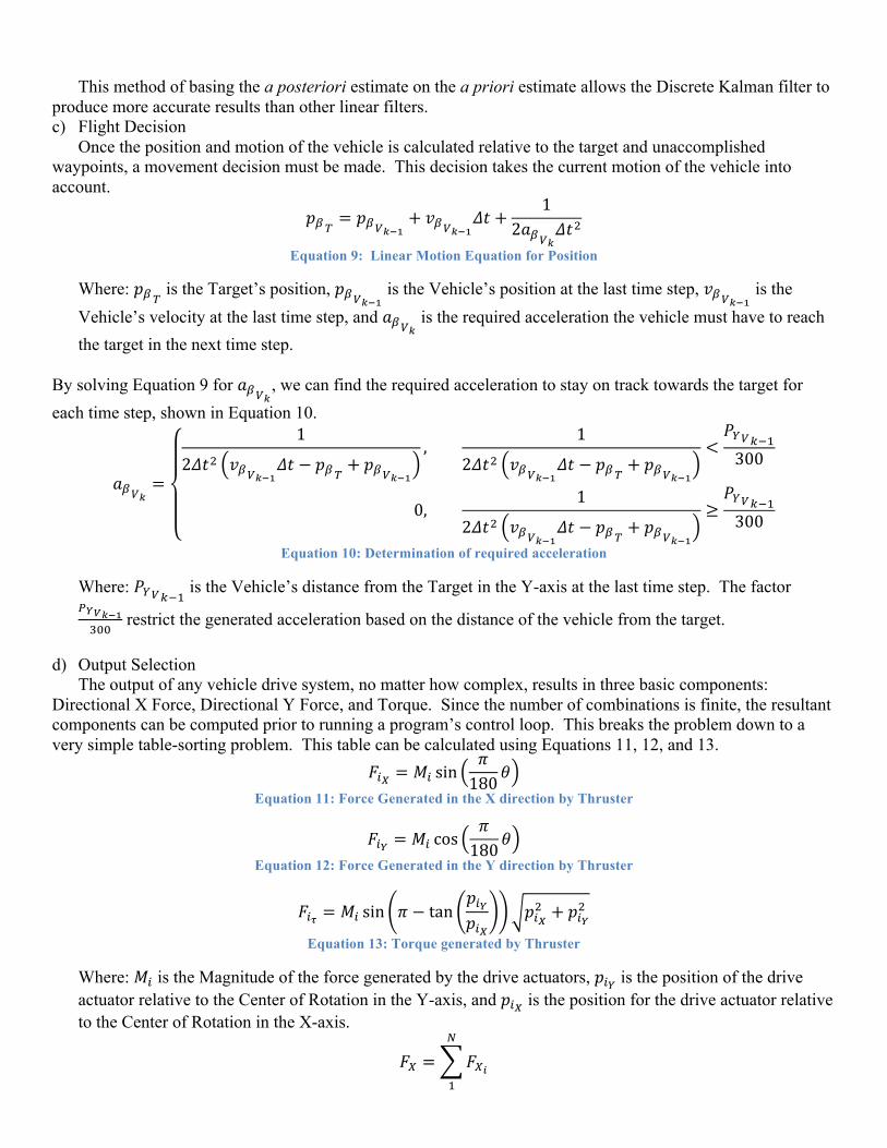
Once the position and motion of the vehicle is calculated relative to the target and unaccomplished waypoints, a movement decision must be made. This decision takes the current motion of the vehicle into account.

𝑝!! = 𝑝!!!!! + 𝑣!!!!!𝛥𝑡 +1

2𝑎!!!𝛥𝑡!

Equation 9: Linear Motion Equation for Position

Where: 𝑝!! is the Target’s position, 𝑝!!!!! is the Vehicle’s position at the last time step, 𝑣!!!!! is the Vehicle’s velocity at the last time step, and 𝑎!!! is the required acceleration the vehicle must have to reach the target in the next time step.

By solving Equation 9 for 𝑎!!!, we can find the required acceleration to stay on track towards the target for each time step, shown in Equation 10.

𝑎!!! =

1

2𝛥𝑡! 𝑣!!!!!𝛥𝑡 − 𝑝!! + 𝑝!!!!!,

1

2𝛥𝑡! 𝑣!!!!!𝛥𝑡 − 𝑝!! + 𝑝!!!!!<𝑃!!!!!300

0,1

2𝛥𝑡! 𝑣!!!!!𝛥𝑡 − 𝑝!! + 𝑝!!!!!≥𝑃!!!!!300

Equation 10: Determination of required acceleration

Where: 𝑃!!!!! is the Vehicle’s distance from the Target in the Y-axis at the last time step. The factor !!!!!!!""

restrict the generated acceleration based on the distance of the vehicle from the target.

d) Output Selection The output of any vehicle drive system, no matter how complex, results in three basic components:

Directional X Force, Directional Y Force, and Torque. Since the number of combinations is finite, the resultant components can be computed prior to running a program’s control loop. This breaks the problem down to a very simple table-sorting problem. This table can be calculated using Equations 11, 12, and 13.

𝐹!! = 𝑀! sin𝜋180𝜃

Equation 11: Force Generated in the X direction by Thruster

𝐹!! = 𝑀! cos𝜋180𝜃

Equation 12: Force Generated in the Y direction by Thruster

𝐹!! = 𝑀! sin 𝜋 − tan𝑝!!𝑝!!

𝑝!!! + 𝑝!!

!

Equation 13: Torque generated by Thruster

Where: 𝑀! is the Magnitude of the force generated by the drive actuators, 𝑝!! is the position of the drive actuator relative to the Center of Rotation in the Y-axis, and 𝑝!! is the position for the drive actuator relative to the Center of Rotation in the X-axis.

𝐹! = 𝐹!!

!

!

Equation 14: Resultant force in the X direction

𝐹! = 𝐹!!

!

!

Equation 15: Resultant force in the Y direction

𝐹! = 𝐹!!

!

!

Equation 16: Resultant rotational force

Where: N is the number of drive actuators.

Associated with each table entry is the drive decision and it’s three generated components. To choose the drive actuator combination that accomplishes the required output, a fitness function is used to evaluate the fitness of each entry using the Euclidian distance from the required components. Then, the combination associated with the lowest (“fittest”) function will be sent as the output from the system.

𝑓! = 𝐹!! − 𝐹!!"#$%&"' + 𝐹!! − 𝐹!!"#$%&"' + 𝐹!! − 𝐹!!"#$%&"' Equation 17: Fitness equation to judge table entries

𝑑𝑒𝑐𝑖𝑠𝑖𝑜𝑛!"#$"# = 𝑑𝑒𝑐𝑖𝑠𝑖𝑜𝑛! , min!!!!!𝑓!

Equation 18: Decision selection based on minimum fitness

III. System Integration Each algorithm plays an important part in the overall roll of the Guidance, Navigation and Control system. The program flow can be seen in Figure 2. First the motion & position of the vehicle is measured from its sensors. The measurement is then filtered to produce estimates for the position, velocity, and acceleration for each degree of freedom. Based on this measurement, if the current waypoint has been reached the next waypoint will be selected. Otherwise, the current waypoint is maintained. Based on the difference of position between the vehicle and the waypoint, as well as the vehicle’s current motion, a decision is made as to what acceleration needs to be applied to the vehicle. This acceleration is then used to determine which drive actuators are used to accomplish this required output based on a best fitness selection. Then, the loop

runs through again. The vehicle used to conduct our tests was a 1.5-ton air-bearing vehicle with 18 thrusters used as drive actuators. Each thruster could output either 1-pound of Force, or 3 pounds of Force. The sensor used to compute the vehicle’s position in relation to the target was the VGS tested in space already to measure relative position from a target. At the time of this writing the autonomous flight decision module was still in the debugging stages. However, we were able to run tests to compare a human pilot’s ability to dock the vehicle with the target using the thruster selection algorithm, referred to as 3DOF for short. The control test was a more traditional drive method that fires all the thrusters on the axis of motion, modifying motion only one axis at a time. This method is referred to as 2DOF.

IV. Results

A total of 32 tests were conducted by the pilot, half being 2DOF flights and half being 3DOF flights. The results indicate that the 2DOF method, at least with manual control, performs better. It took a human pilot on average 71.03% of the time it took to dock using the 3DOF method to dock using the 2DOF method. Logically,

Posi%on  Measurement  

Posi%on  Calcula%on  

(Kalman  Filter)  

Waypoint  Selec%on  Flight  Decision  

Output  Selec%on  

Figure 2: Autonomous Program Flow

this will equate to the 2DOF method consuming less total air, 36.82% of the air used with the 3DOF method. These results can be seen in Figures 3 & 4. However, after further analysis of the thruster firings, it became apparent that regardless of the shorter docking time, the 2DOF thruster method was consuming less air, as could be seen in Figure 5. In addition to using more air than the control test, the 3DOF test also had more total error across all axes of movement. In other words, on average it was farther off track than the 2DOF control test, as seen in Figure 6.

V. Conclusions Considering a human pilot did the tests, it is possible to consign the negative results to a higher learning curve than expected. However, if we consider the construction of the algorithm, it called for thrusters to fire to minimize any unwanted directional or rotational force. With the 2DOF, this could be corrected for by the application of a quick overcorrection in the opposite direction. In addition, the 3DOF system reduced the drive force in any one-degree of freedom, as it tried to control all of the degrees of freedom. The algorithm is on the right track. However, in order to be more efficient, the user interface (an Xbox controller) and the fitness measure needs refinement.

Bibliography  Welch, Greg and Gary Bishop. "An Introduction to the Kalman Filter." 24 July 2006. Department of Computer Science, UNC-Chapel Hill. 25 July 2011 <http://www.cs.unc.edu/~welch/media/pdf/kalman_intro.pdf>. —. The Kalman Filter. 3 July 2011. 25 July 2011 <http://www.cs.unc.edu/~welch/kalman/>. Wikimedia Foundation. "Logistic Function." 26 May 2011. Wikipedia, The Free Encyclopedia. 25 July 2011 <http://en.wikipedia.org/wiki/Logistic_function>. Esme, Bilgin. "Kalman Filter for Dummies." 1 March 2009. Bilgin's Blog. 25 July 2011 <http://bilgin.esme.org/BitsBytes/KalmanFilterforDummies.aspx>. Fehse, Wigbert. Automated Rendezvous and Docking of Spacecraft. Cambridge: Cambridge University Press, 2003.

50  

55  

60  

65  

70  

75  

80  

85  

90  

95  

100  

3DOF   2DOF  

Time  required  for  docking  (s)  

Avg.  +/-­‐  3σ  

Figure 3: Average Time to Dock

0  

1  

2  

3  

4  

5  

6  

3DOF   2DOF  

Air  consumed  (kg)  

Avg.  +/-­‐  3σ  

Figure 4: Average Air Consumed

Figure 5: Air Consumption over Time

-­‐1  

0  

1  

2  

3  

4  

5  

6  

7  

8  

0   20   40   60   80   100   120  

Air  (kg)  

Time  (s)  

Air  consump:on  over  :me  

3DOF  

2DOF  

0  

1  

2  

3  

4  

5  

6  

0   20   40   60   80   100   120  

Time  (s)  

Error  over  :me  

3DOF  

2DOF  

Figure 6: Error over Time