Submitted 4 August 2017Accepted 10 April 2018Published 28 May 2018

Corresponding authorJ. Frederico Carvalho, jfpbdc@kth.se

Academic editorMark Wilson

Additional Information andDeclarations can be found onpage 11

DOI 10.7717/peerj-cs.153

Copyright2018 Carvalho et al.

Distributed underCreative Commons CC-BY 4.0

OPEN ACCESS

An algorithm for calculating top-dimensional bounding chainsJ. Frederico Carvalho1, Mikael Vejdemo-Johansson2, Danica Kragic1 andFlorian T. Pokorny1

1CAS/RPL, KTH, Royal Institute of Technology, Stockholm, Sweden2Mathematics Department, City University of New York, College of Staten Island, New York, NY,United States of America

ABSTRACTWe describe theCoefficient-Flow algorithm for calculating the bounding chain of an(n−1)-boundary on an n-manifold-like simplicial complex S. We prove its correctnessand show that it has a computational time complexity of O(|S(n−1)|) (where S(n−1)

is the set of (n− 1)-faces of S). We estimate the big-O coefficient which dependson the dimension of S and the implementation. We present an implementation,experimentally evaluate the complexity of our algorithm, and compare its performancewith that of solving the underlying linear system.

Subjects Algorithms and Analysis of Algorithms, Data Science, Scientific Computing andSimulationKeywords Homology, Computational algebraic topology

INTRODUCTIONTopological spaces are by and large characterized by the cycles in them (i.e., closed pathsand their higher dimensional analogues) and the ways in which they can or cannot bedeformed into each other. This idea had been recognized by Poincaré from the beginningof the study of topology. Consequently much of the study of topological spaces has beendedicated to understanding cycles, and these are the key features studied by the topologicaldata analysis community (Edelsbrunner & Harer, 2010).

One key part of topological data analysis methods is to distinguish between differentcycles; more precisely, to characterize different cycles according to their homology class.This can be done efficiently using cohomology (Pokorny, Hawasly & Ramamoorthy, 2016;Edelsbrunner, Letscher & Zomorodian, 2002). However, such methods only distinguishbetween non-homologous cycles, and do not quantify the difference between cycles. Apossible way to quantify this difference is to solve the problem of finding the chain whoseboundary is the union of the two cycles in question, as was proposed in Chambers &Vejdemo-Johansson (2015) by solving the underlying linear system, where the authorsalso take the question of optimality into account (with regards to the size of the resultingchain). This line of research ellaborates onDey, Hirani & Krishnamoorthy (2011) where theauthors considered the problem of finding an optimal chain in the same homology classas a given chain. More recently, in Rodríguez et al. (2017) the authors have taken a similarapproach to ours using a combinatorial method to compute bounding chains of 1-cycleson 3-dimensional simplicial complexes.

How to cite this article Carvalho et al. (2018), An algorithm for calculating top-dimensional bounding chains. PeerJ Comput. Sci.4:e153; DOI 10.7717/peerj-cs.153

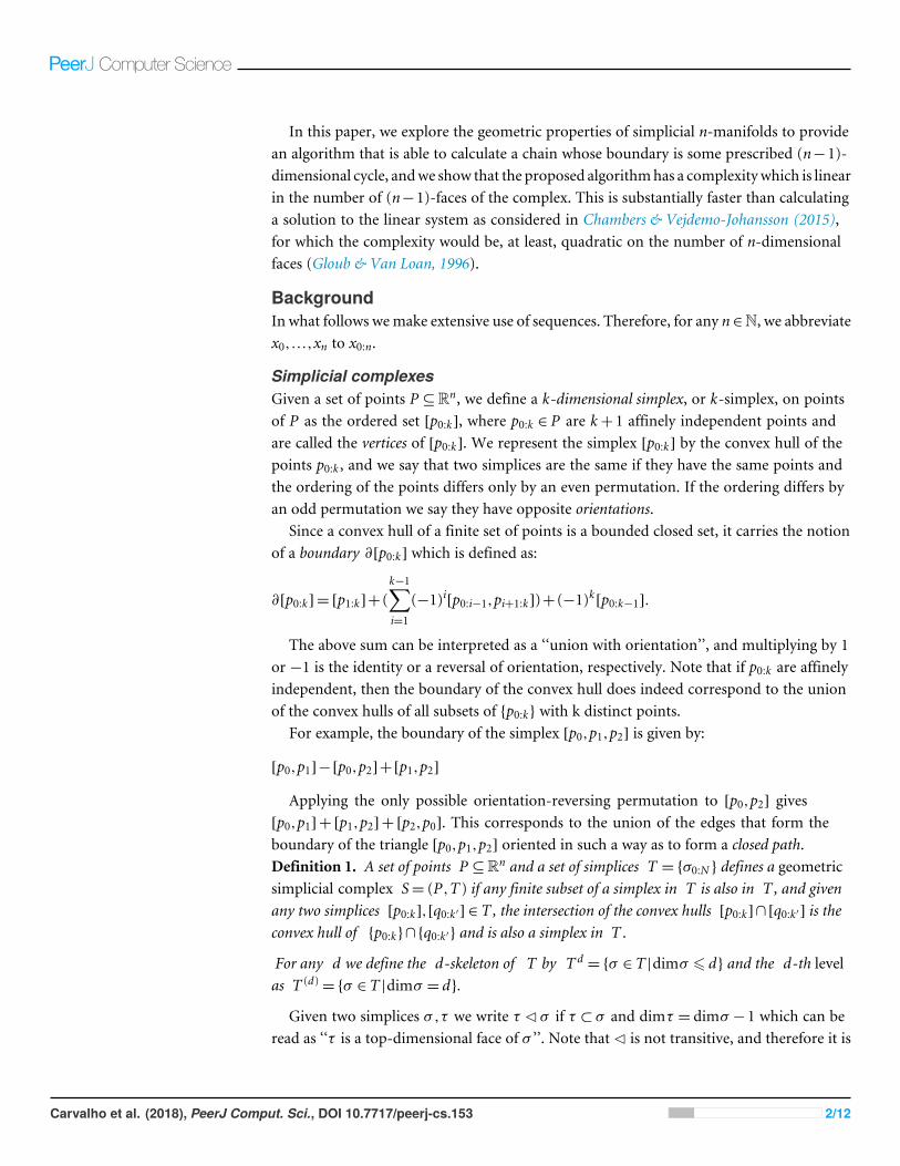
In this paper, we explore the geometric properties of simplicial n-manifolds to providean algorithm that is able to calculate a chain whose boundary is some prescribed (n−1)-dimensional cycle, andwe show that the proposed algorithmhas a complexitywhich is linearin the number of (n−1)-faces of the complex. This is substantially faster than calculatinga solution to the linear system as considered in Chambers & Vejdemo-Johansson (2015),for which the complexity would be, at least, quadratic on the number of n-dimensionalfaces (Gloub & Van Loan, 1996).

BackgroundIn what follows wemake extensive use of sequences. Therefore, for any n∈N, we abbreviatex0,...,xn to x0:n.

Simplicial complexesGiven a set of points P ⊆Rn, we define a k-dimensional simplex, or k-simplex, on pointsof P as the ordered set [p0:k], where p0:k ∈ P are k+1 affinely independent points andare called the vertices of [p0:k]. We represent the simplex [p0:k] by the convex hull of thepoints p0:k , and we say that two simplices are the same if they have the same points andthe ordering of the points differs only by an even permutation. If the ordering differs byan odd permutation we say they have opposite orientations.

Since a convex hull of a finite set of points is a bounded closed set, it carries the notionof a boundary ∂[p0:k] which is defined as:

∂[p0:k] = [p1:k]+ (k−1∑i=1

(−1)i[p0:i−1,pi+1:k])+ (−1)k[p0:k−1].

The above sum can be interpreted as a ‘‘union with orientation’’, and multiplying by 1or −1 is the identity or a reversal of orientation, respectively. Note that if p0:k are affinelyindependent, then the boundary of the convex hull does indeed correspond to the unionof the convex hulls of all subsets of {p0:k} with k distinct points.

For example, the boundary of the simplex [p0,p1,p2] is given by:

[p0,p1]−[p0,p2]+[p1,p2]

Applying the only possible orientation-reversing permutation to [p0,p2] gives[p0,p1]+ [p1,p2]+ [p2,p0]. This corresponds to the union of the edges that form theboundary of the triangle [p0,p1,p2] oriented in such a way as to form a closed path.Definition 1. A set of points P ⊆Rn and a set of simplices T = {σ0:N } defines a geometricsimplicial complex S= (P,T ) if any finite subset of a simplex in T is also in T , and givenany two simplices [p0:k],[q0:k ′] ∈ T, the intersection of the convex hulls [p0:k]∩ [q0:k ′] is theconvex hull of {p0:k}∩{q0:k ′} and is also a simplex in T .

For any d we define the d-skeleton of T by T d= {σ ∈T |dimσ 6 d} and the d-th level

as T (d)={σ ∈T |dimσ = d}.

Given two simplices σ ,τ we write τ C σ if τ ⊂ σ and dimτ = dimσ −1 which can beread as ‘‘τ is a top-dimensional face of σ ’’. Note that C is not transitive, and therefore it is

Carvalho et al. (2018), PeerJ Comput. Sci., DOI 10.7717/peerj-cs.153 2/12

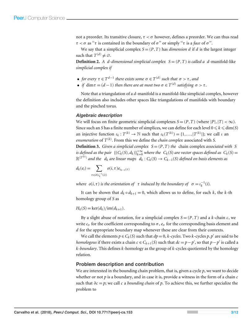
not a preorder. Its transitive closure, τ <σ however, defines a preorder. We can thus readτ <σ as ‘‘τ is contained in the boundary of σ ’’ or simply ‘‘τ is a face of σ ’’.

We say that a simplicial complex S= (P,T ) has dimension d if d is the largest integersuch that T (d)

6=∅.Definition 2. A d-dimensional simplicial complex S= (P,T ) is called a d-manifold-likesimplicial complex if

• for every τ ∈T d−1 there exists some σ ∈T (d) such that σ > τ , and• if dimτ = (d−1) then there are at most two σ ∈T (d) satisfying σ > τ .

Note that a triangulation of a d-manifold is a manifold-like simplicial complex, howeverthe definition also includes other spaces like triangulations of manifolds with boundaryand the pinched torus.

Algebraic descriptionWe will focus on finite geometric simplicial complexes S= (P,T ) (where |P|,|T |<∞).Since such an S has a finite number of simplices, we can define for each level 06 k6 dim(S)an injective function ιk : T (k)

→ N such that ιk(T (k))= {1,...,|T (k)|}; we call ι an

enumeration of T (k). From this we define the chain complex associated with S.Definition 3. Given a simplicial complex S= (P,T ) the chain complex associated with Sis defined as the pair {(Ck(S),dk)}+∞k=0 where the Ck(S) are vector spaces defined as Ck(S)=R|T (k)

| and the dk are linear maps dk : Ck(S)→ Ck−1(S) defined on basis elements as

dk(ei)=∑

τ∈∂(ι−1k (i))

o(i,τ )eιk−1(τ )

where o(i,τ ) is the orientation of τ induced by the boundary of σ = ι−1k (i).

It can be shown that dk ◦ dk+1 = 0, which allows us to define, for each k, the k-thhomology group of S as

Hk(S)= ker(dk)/im(dk+1).

By a slight abuse of notation, for a simplicial complex S= (P,T ) and a k-chain c , wewrite cσ for the coefficient corresponding to σ , eσ for the corresponding basis element andd for the appropriate boundary map whenever these are clear from their contexts.

We call the elements p∈Ck(S) such that dp= 0, k-cycles. Two k-cycles p,p′ are said to behomologous if there exists a chain c ∈Ck+1(S) such that dc = p−p′, so that p−p′ is called ak-boundary. This defines k-homology as the group of k-cycles quotiented by the homologyrelation.

Problem description and contributionWe are interested in the bounding chain problem, that is, given a cycle p, we want to decidewhether or not p is a boundary, and in case it is, provide a witness in the form of a chain csuch that ∂c = p; we call c a bounding chain of p. To achieve this, we further specialize theproblem to

Carvalho et al. (2018), PeerJ Comput. Sci., DOI 10.7717/peerj-cs.153 3/12

1Which corresponds to the number of(k − 1)- and k-faces of the complex,respectively.

solve: ∂c = p

subject to: cσ = v, (1)

where p is a specified (n−1)-boundary in an n-manifold-like simplicial complex S, σ isan n-simplex, and v is a pre-specified real number. In general, the equation ∂c = p hasmore than one solution c , therefore by adding the constraint cσ = v we are able to makethis solution unique.

The Coefficient-Flow algorithm that we present solves this restricted form of thebounding chain problem (by providing one such bounding chain if it exists) and hascomputational time complexity of O(|S(n−1)|). Furthermore, we show how the parametersσ and v can be done away with in cases where the chain is unique, and we discuss how thisalgorithm can be used to find a minimal bounding chain.

Related workIn Chambers & Wang (2013) the authors address the problem of computing the areaof a homotopy between two paths on 2-dimensional manifolds, which can be seenas a generalization of the same problem, for 2-dimensional meshes via the Hurewiczmap (Hatcher, 2002). In Chambers & Vejdemo-Johansson (2015) the authors provide amethod for calculating the minimum area bounding chain of a 1-cycle on a 2d mesh, thatis the solution to the problem

argmin carea(c)= p, where ∂c = p (2)

and p is a 1-chain on a given simplicial complex. This is done by using optimizationmethodsfor solving the associated linear system. These methods however have time complexitylower-bounded by matrix multiplication time which is in �(min(n,m)2) where n,m arethe number of rows and columns of the boundary matrix1 (Davie & Stothers, 2013). Thiscomplexity quickly becomes prohibitive when we handle large complexes, such as onemight find when dealing with meshes constructed from large pointclouds.

More recently, in Rodríguez et al. (2017) the authors proposed a method for computingbounding chains of 1-cycles in 3-dimensional complexes, using a spanning tree of the dualgraph of the complex.

In Dey, Hirani & Krishnamoorthy (2011) the authors address the related problem ofefficiently computing an optimal cycle p′ which is homologous to a given cycle p (with Zcoefficients). This is a significant result given that in Chambers, Erickson & Nayyeri (2009)the authors proved that this cannot be done efficiently (i.e., in polynomial time) for 1-cyclesusing Z2 coefficients, a result that was extended in Chen & Freedman (2011) to cycles ofany dimension.

METHODOLOGYFor any simplicial complex S, and any pair of simplices σ ,τ ∈ S such that, τ C σ , we definethe index of τ with respect to σ as 〈τ ,∂σ 〉= 〈eτ ,deσ 〉 (Forman, 1998). Note that the indexcorresponds to the orientation induced by the boundary of σ on τ and can be computedin O(d) time by the following algorithm:

Carvalho et al. (2018), PeerJ Comput. Sci., DOI 10.7717/peerj-cs.153 4/12

Index(σ ,τ ):param: σ - k-simplex represented as a sorted list of indices of points.param: τ - (k−1)-face of σ represented as a sorted list of indices.

1: for each i← 0...dimτ :2: if τi 6= σi:3: orientation← (−1)i

4: break loop5: return orientation

By inspecting the main loop we can see that Index(σ ,τ ) returns (−1)i where i is theindex of the first element at which σ and τ differ. We assume τ is a top dimensional face ofσ , so if σ = [s0:d], then by definition τ = [s0:(i−1),s(i+1):d] for some i, and so the coefficientof τ in the boundary of σ is (−1)i as per the definition of the boundary operator. This isalso the index of the first element at which τ and σ differ, since they are represented assorted lists of indices.

The following is an intuitive result, that will be the basis for the Coefficient-Flowalgorithm that we will present in the sequel.Proposition 1. Let S be a manifold-like simplicial complex, let c be an n-chain on S andp its boundary. Then for any pair of n-simplices σ 6= σ ′ with ∂σ ∩∂σ ′={τ } we have:

cσ =〈τ ,∂σ 〉(pτ −〈τ ,∂σ ′〉cσ ′).

Proof. If we expand the equation ∂c = p, we get pτ =∑

τCω〈eτ ,d(cωeω)〉, recall that bydefinition d(cωeω)=

∑νCω〈ν,∂ω〉cωeν ; and so we get pτ =

∑τCω〈τ ,∂ω〉cωeτ .

Now since S is a manifold-like simplicial complex and τ = ∂σ ∩∂σ ′, then σ ,σ ′ are theonly cofaces of τ , and hence we have:

pτ =〈τ ,∂σ 〉cσ +〈τ ,∂σ ′〉cσ ′

which can be reorganized to cσ =pτ−〈τ ,∂σ ′〉cσ ′〈τ ,∂σ 〉

. Finally, since the index 〈τ ,∂σ 〉 is either 1or −1, we can rewrite this equation as:

cσ =〈τ ,∂σ 〉(pτ −〈τ ,∂σ ′〉cσ ′)

Next, we present an algorithm to calculate a bounding chain for a (n− 1)-cycle inan n-manifold-like simplicial complex. The algorithm proceeds by checking every top-dimensional face σ , and calculating the value of the chain on adjacent top-dimensionalfaces, using Proposition 1.

In order to prove that the Coefficient-Flow algorithm solves problem (1), will use thefact that we can see the algorithm as a traversal of the dual graph.Definition 4. Given an n-dimensional simplicial complex S, recall that the dual graph is agraph G(S)= (V ,E) with set of vertices V = S(n) and (σ ,σ ′)∈ E if dim(σ ∩σ ′)= n−1.

Proposition 2. If S is a manifold-like simplicial complex, where G(S) is connected, and pis an (n−1)-boundary, then Coefficient- Flow(p,σ ,v) returns a bounding chain c of psatisfying cσ = v, if such a boundary exists. Furthermore, the main loop (05–21) is executedat most O(|S(n−1)|) times.

Carvalho et al. (2018), PeerJ Comput. Sci., DOI 10.7717/peerj-cs.153 5/12

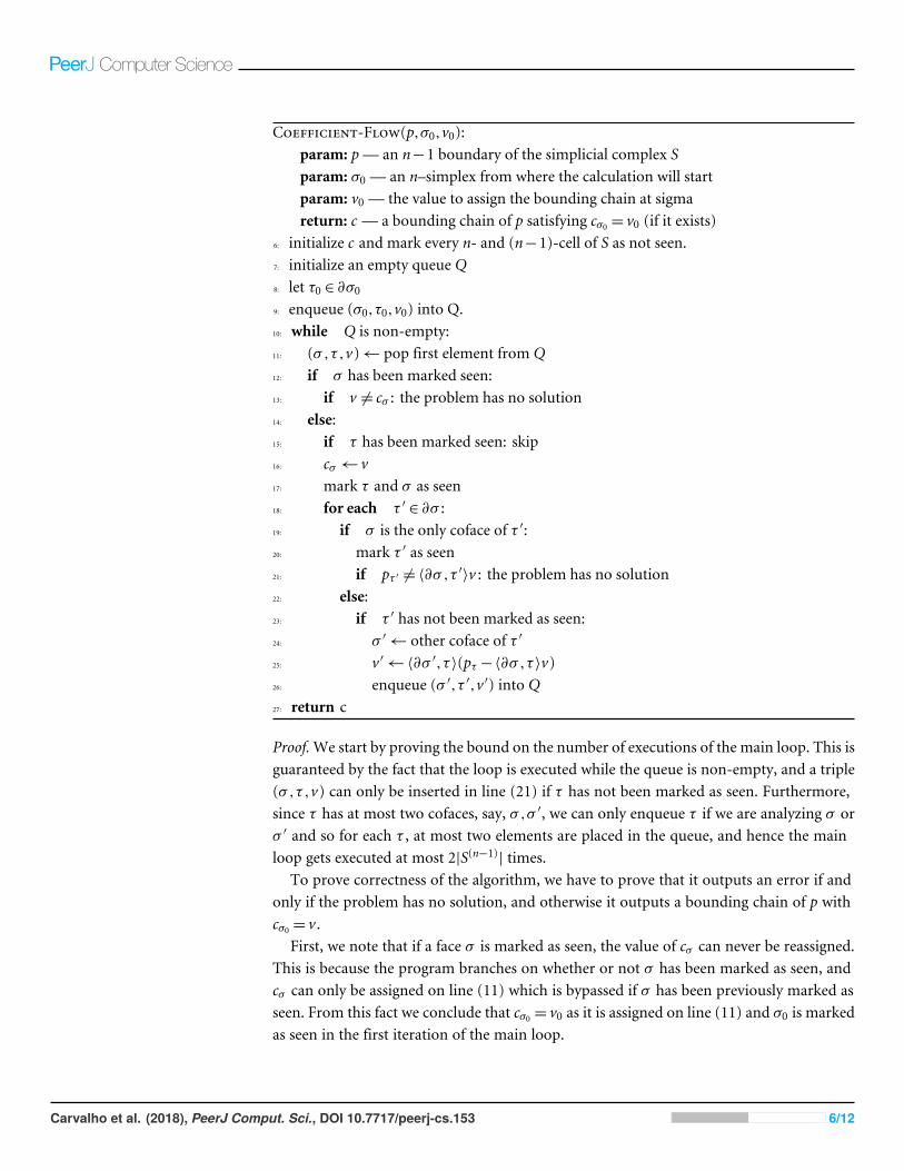
Coefficient-Flow(p,σ0,v0):param: p— an n−1 boundary of the simplicial complex Sparam: σ0 — an n–simplex from where the calculation will startparam: v0 — the value to assign the bounding chain at sigmareturn: c — a bounding chain of p satisfying cσ0 = v0 (if it exists)

6: initialize c and mark every n- and (n−1)-cell of S as not seen.7: initialize an empty queue Q8: let τ0 ∈ ∂σ09: enqueue (σ0,τ0,v0) into Q.10: while Q is non-empty:11: (σ ,τ ,v)← pop first element from Q12: if σ has been marked seen:13: if v 6= cσ : the problem has no solution14: else:15: if τ has been marked seen: skip16: cσ← v17: mark τ and σ as seen18: for each τ ′ ∈ ∂σ :19: if σ is the only coface of τ ′:20: mark τ ′ as seen21: if pτ ′ 6= 〈∂σ ,τ ′〉v : the problem has no solution22: else:23: if τ ′ has not been marked as seen:24: σ ′← other coface of τ ′

25: v ′←〈∂σ ′,τ 〉(pτ −〈∂σ ,τ 〉v)26: enqueue (σ ′,τ ′,v ′) into Q27: return c

Proof.We start by proving the bound on the number of executions of the main loop. This isguaranteed by the fact that the loop is executed while the queue is non-empty, and a triple(σ ,τ ,v) can only be inserted in line (21) if τ has not been marked as seen. Furthermore,since τ has at most two cofaces, say, σ ,σ ′, we can only enqueue τ if we are analyzing σ orσ ′ and so for each τ , at most two elements are placed in the queue, and hence the mainloop gets executed at most 2|S(n−1)| times.

To prove correctness of the algorithm, we have to prove that it outputs an error if andonly if the problem has no solution, and otherwise it outputs a bounding chain of p withcσ0 = v .

First, we note that if a face σ is marked as seen, the value of cσ can never be reassigned.This is because the program branches on whether or not σ has been marked as seen, andcσ can only be assigned on line (11) which is bypassed if σ has been previously marked asseen. From this fact we conclude that cσ0 = v0 as it is assigned on line (11) and σ0 is markedas seen in the first iteration of the main loop.

Carvalho et al. (2018), PeerJ Comput. Sci., DOI 10.7717/peerj-cs.153 6/12

Second, note that there is an edge between two n-faces in the dual graph if and only ifthey share an (n−1)-face. This implies that as we execute the algorithm, analyze a newn-face σ and successfully add the other cofaces of elements of the boundary of σ , we addthe vertices neighboring σ in the dual graph. Since the dual graph is connected all of thenodes in the graph are eventually added, and hence all of the n-faces are analyzed.

Third, we note that for any pair (τ ,σ ) with dimσ = n and τ C σ , either σ is the onlycoface of τ , or τ has another coface, σ ′. In the first case, if pτ 6= cσ 〈τ ,∂σ 〉 an error isdetected on line (16). In the second case, assuming that the triple (σ ,τ ,v) is enqueuedbefore (σ ′,τ ,v ′) we have v ′=〈∂σ ′,τ 〉(pτ −〈∂,σ 〉v) as is assigned in line (20) then

(dc)τ =〈∂σ ,τ 〉v+〈∂σ ′,τ 〉v ′

=〈∂σ ,τ 〉v+〈∂σ ′,τ 〉(〈∂σ ′,τ 〉(pτ −〈∂,σ 〉v))

=〈∂σ ,τ 〉v+pτ −〈∂σ ,τ 〉v = pτ .

Finally, since upon the successful return of the algorithm, this equation must be satisfiedby every pair τ C σ , it must be the case that dc = p. If this is not the case, then there will bean error in line (08) and the algorithm will abort. �

Note that the connectivity condition can be removed if we instead require a value forone cell in each connected component of the graph G(S), and throw an error in case thereis an (n−1)-simplex τ with no cofaces, such that pτ 6= 0. Furthermore, the algorithm canbe easily parallelized using a thread pool that iteratively processes elements from the queue.

Finally, in the case where it is known that S has an (n−1)-face τ with a single coface,we do not need to specify σ or v in Coefficient-Flow, and instead use the fact that weknow the relationship between the coefficient pτ and that of its coface in a bounding chainc of p, i.e., pτ =〈∂σ ,τ 〉cσ . This proves Corollary 1.

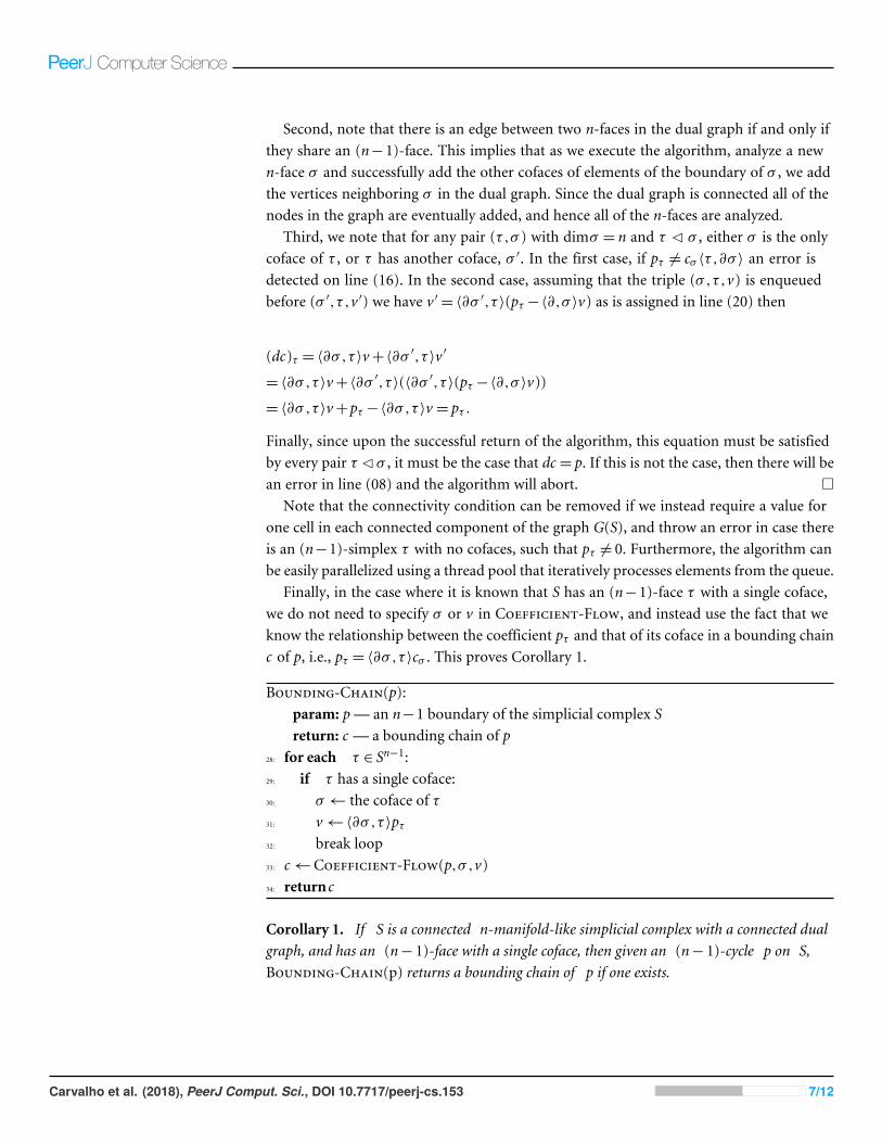
Bounding-Chain(p):param: p— an n−1 boundary of the simplicial complex Sreturn: c — a bounding chain of p

28: for each τ ∈ Sn−1:29: if τ has a single coface:30: σ← the coface of τ31: v←〈∂σ ,τ 〉pτ32: break loop33: c←Coefficient-Flow(p,σ ,v)34: return c

Corollary 1. If S is a connected n-manifold-like simplicial complex with a connected dualgraph, and has an (n− 1)-face with a single coface, then given an (n− 1)-cycle p on S,Bounding-Chain(p) returns a bounding chain of p if one exists.

Carvalho et al. (2018), PeerJ Comput. Sci., DOI 10.7717/peerj-cs.153 7/12

Implementation detailsWe will now discuss some of the choices made in our implementation of the Coefficient-Flow algorithm (https://www.github.com/crvs/coeff-flow). Before we can address theproblem of considering chains on a simplicial complex we first need to have a model of asimplicial complex. For this, we decided to use a simplex tree model (Boissonnat & Maria,2014) provided by the GUDHI library (The GUDHI Project, 2015) as it provides a compactrepresentation of a simplicial complex (the number of nodes in the tree is in bijection withthe number of simplices) which allows us to quickly get the enumeration of a given simplexσ . Indeed, the complexity of calculating ιk(σ ) is in O(dimσ ).

It is important to compute the enumeration quickly because in our implementation ofCoefficient-Flow we use arrays of booleans to keep track of which faces of the simplicialcomplex have been seen before, as well as numerical arrays to store the coefficients of thecycle and its bounding chain, which need to be consulted at every iteration of the loop.

However, finding the cofaces of the simplicial complex is not as easy in a simplex tree,since, if σ = [pi0:ik ], this would require to search every child of the root node of the treethat has an index smaller than i0, followed by every child of the node associated with pi0and so on, which in the worst case scenario is in O(dimσ |S(0)|). Thus we need to adopt adifferent method. For this, we keep a Hasse diagram of the face relation which comprises adirected graph whose vertices are nodes in the simplex tree and has edges from each face toits codimension-1 cofaces (see for instance Di Battista & Tamassia (1988)) for more detailsof this data-structure). This allows us to find the codimension-1 cofaces of a simplex of Sin O(1) with a space overhead in O(|S|).

With these elements in place, we can analyze the complexity of our implementation ofthe Coefficient-Flow algorithm in full:Lemma 1. The Coefficient-Flow algorithm using a simplex tree and a Hasse diagram hascomputational (time) complexity O(d2|S(d−1)|) where d = dimS.

Proof. In Proposition 2 we saw that the Coefficient-Flow algorithm executes the main loopat most O(|S(d)|) times, so we only need to measure the complexity of the main loop, inorder to obtain its time complexity. This can be done by checking which are the costlysteps:

• In lines (07) and (10) checking whether a face has been marked as seen requires firstcomputing ιk(τ ) which, as we stated above, has time complexity O(k), with k ≤ d .• In line (13), computing the faces of a simplex σ requires O(dimσ 2) steps, and yields alist of size dimσ , hence the inner loop (13–21) is executed dimσ times, where dimσ = d ,for each element placed in the queue.• The loop (13–21) requires once again, computing ι(τ ′), and 〈∂σ ,τ 〉, each of theseoperations, as we explained before, carries a time complexity O(d).• All other operations have complexity O(1).

Composing these elements, the total complexity of one iteration of the main loopis O(max{d,d2,d · d}) = O(d2), which yields a final complexity for the proposedimplementation, of O(d2|S(d−1)|). �

Carvalho et al. (2018), PeerJ Comput. Sci., DOI 10.7717/peerj-cs.153 8/12

2We use the least squares conjugategradient descent method to solve thesystem.

Figure 1 Examples of bounding chains: the edges in blue form cycles in the mesh, and the faces in redform the corresponding bounding chain as computed by the Coefficient-Flow algorithm. In (A) wedepict the mesh of the Stanford Bunny The Stanford 3D scanning repository (1994) and in (B) we show themesh of a Bee Smithsonian (2013). In both these meshes we depict examples of bounding chains, wherethe edges in blue form cycles, and the faces in red form the corresponding bounding chain as computedby the Coefficient-Flow algorithm. In both cases the depicted bounding chains correspond to the op-timal bounding chains (w.r.t. the number of faces), these can by obtained by choosing σ0 and v0 so as toyield the desired chain. In this case, since the two complexes are topological spheres and the cycles are sim-ple cycles (meaning they are connected and do not self-intersect), there are only two possible boundingchains that do not include all the faces of the complex, which can be obtained by running the algorithmthree times, choosing σ0 arbitrarily, and setting v0 to be 0,n or−n where n =maxτ∈S(1) |pτ |. In the case ofnon-simple cycles, more alternatives would exist.

Full-size DOI: 10.7717/peerjcs.153/fig-1

Example runs and testsIn Fig. 1 we provide an example of the output of the Coefficient-Flow algorithm for themesh of the Stanford bunny (The Stanford 3D scanning repository, 1994) and the eulaemameriana bee model from the Smithsonian 3D model library (Smithsonian, 2013).

For comparison, we performed the same experiments using the Eigen linear algebralibrary (Eigen, 2017) to solve the underlying linear system,2 and summarized the resultsin Table 1. This allowed us to see that even though both approaches remain feasible withrelatively large meshes, solving the linear system consistently underperforms using theCoefficient-Flow algorithm.

Even though Coefficient-Flow is expected to outperform a linear system solver (anexact solution to a linear system has�(n2) time complexity), we wanted to test it against anapproximate sparse system solver. Such solvers (e.g., conjugate gradient descent (Gloub &Van Loan, 1996)) rely on iterative matrix products, which in the case of boundary matricesof dimension d can be performed in O((d+1)n) where n is the number of d-dimensionalsimplices, placing the complexity of the method in �((d+1)n). In order to observe thedifference in complexity class we performed randomized tests on both implementations.

Carvalho et al. (2018), PeerJ Comput. Sci., DOI 10.7717/peerj-cs.153 9/12

3Since boundary matrices are naturallysparse, and we are computing anapproximate solution, the complexity canbe improved beyond the aforementioned�(n2).

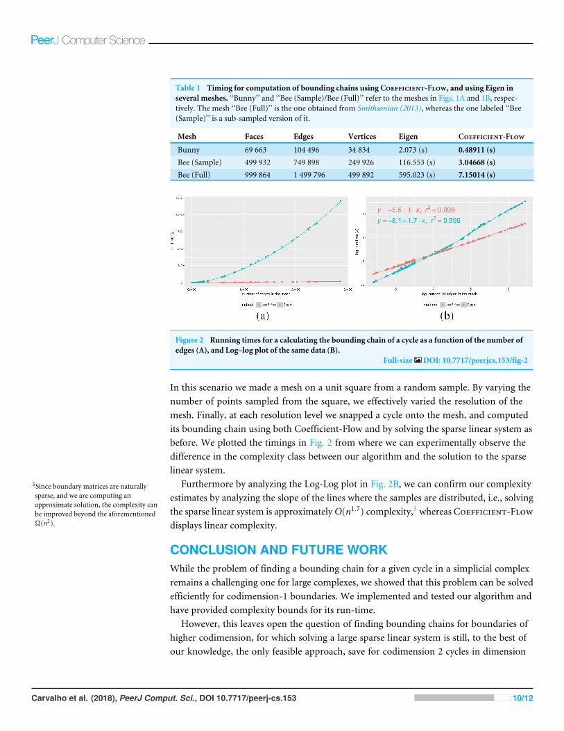
Table 1 Timing for computation of bounding chains using Coefficient-Flow, and using Eigen inseveral meshes. ‘‘Bunny’’ and ‘‘Bee (Sample)/Bee (Full)’’ refer to the meshes in Figs. 1A and 1B, respec-tively. The mesh ‘‘Bee (Full)’’ is the one obtained from Smithsonian (2013), whereas the one labeled ‘‘Bee(Sample)’’ is a sub-sampled version of it.

Mesh Faces Edges Vertices Eigen Coefficient-Flow

Bunny 69 663 104 496 34 834 2.073 (s) 0.48911 (s)Bee (Sample) 499 932 749 898 249 926 116.553 (s) 3.04668 (s)Bee (Full) 999 864 1 499 796 499 892 595.023 (s) 7.15014 (s)

Figure 2 Running times for a calculating the bounding chain of a cycle as a function of the number ofedges (A), and Log–log plot of the same data (B).

Full-size DOI: 10.7717/peerjcs.153/fig-2

In this scenario we made a mesh on a unit square from a random sample. By varying thenumber of points sampled from the square, we effectively varied the resolution of themesh. Finally, at each resolution level we snapped a cycle onto the mesh, and computedits bounding chain using both Coefficient-Flow and by solving the sparse linear system asbefore. We plotted the timings in Fig. 2 from where we can experimentally observe thedifference in the complexity class between our algorithm and the solution to the sparselinear system.

Furthermore by analyzing the Log-Log plot in Fig. 2B, we can confirm our complexityestimates by analyzing the slope of the lines where the samples are distributed, i.e., solvingthe sparse linear system is approximatelyO(n1.7) complexity,3 whereas Coefficient-Flowdisplays linear complexity.

CONCLUSION AND FUTURE WORKWhile the problem of finding a bounding chain for a given cycle in a simplicial complexremains a challenging one for large complexes, we showed that this problem can be solvedefficiently for codimension-1 boundaries. We implemented and tested our algorithm andhave provided complexity bounds for its run-time.

However, this leaves open the question of finding bounding chains for boundaries ofhigher codimension, for which solving a large sparse linear system is still, to the best ofour knowledge, the only feasible approach, save for codimension 2 cycles in dimension

Carvalho et al. (2018), PeerJ Comput. Sci., DOI 10.7717/peerj-cs.153 10/12

3 (Rodríguez et al., 2017). In the future we would like to generalize our algorithm to beable to work with cobounding cochains (i.e., in cohomology), as well as considering theoptimality question (i.e., finding the minimal bounding chain w.r.t. some cost function).

ADDITIONAL INFORMATION AND DECLARATIONS

FundingThis work has been supported by the Knut and Alice Wallenberg Foundation and theSwedish Research Council. The funders had no role in study design, data collection andanalysis, decision to publish, or preparation of the manuscript.

Grant DisclosuresThe following grant information was disclosed by the authors:Knut and Alice Wallenberg Foundation.Swedish Research Council.

Competing InterestsThe authors declare there are no competing interests.

Author Contributions• J. Frederico Carvalho conceived and designed the experiments, performed theexperiments, analyzed the data, prepared figures and/or tables, performed thecomputation work, authored or reviewed drafts of the paper, approved the final draft.• Mikael Vejdemo-Johansson, Danica Kragic and Florian T. Pokorny authored or revieweddrafts of the paper.

Data AvailabilityThe following information was supplied regarding data availability:

Github: https://www.github.com/crvs/coeff-flow.

Supplemental InformationSupplemental information for this article can be found online at http://dx.doi.org/10.7717/peerj-cs.153#supplemental-information.

REFERENCESBoissonnat J-D, Maria C. 2014. The simplex tree: an efficient data structure for general

simplicial complexes. Algorithmica 70(3):406–427.Chambers EW, Erickson J, Nayyeri A. 2009.Minimum cuts and shortest homologous

cycles. In: Symposium on Computational geometry DOI 10.1145/1542362.1542426.Chambers EW, Vejdemo-JohanssonM. 2015. Computing minimum area ho-

mologies. In: Computer graphics forum, vol. 34. Wiley Online Library, 13–21DOI 10.1111/cgf.12514.

Carvalho et al. (2018), PeerJ Comput. Sci., DOI 10.7717/peerj-cs.153 11/12

Chambers EW,Wang Y. 2013.Measuring similarity between curves on 2-manifolds viahomotopy area. SoCG ’13. In: Proceeding of the twenty-ninth annual symposium oncomputational geometry. New York: ACM, 425–434 DOI 10.1145/2462356.2462375.

Chen C, Freedman D. 2011.Hardness results for homology localization. Discrete andComputational Geometry 45(3):425–448 DOI 10.1007/s00454-010-9322-8.

Davie AM, Stothers AJ. 2013. Improved bound for complexity of matrix multiplication.Proceedings of the Royal Society of Edinburgh Section A: Mathematics 143(2):351–369DOI 10.1017/S0308210511001648.

Dey TK, Hirani AN, Krishnamoorthy B. 2011. Optimal homologous cycles, total uni-modularity, and linear programming. SIAM Journal on Computing 40(4):1026–1044DOI 10.1137/100800245.

Di Battista G, Tamassia R. 1988. Algorithms for plane representations of acyclicdigraphs. Theoretical Computer Science 61(2) DOI 10.1016/0304-3975(88)90123-5.

Edelsbrunner H, Harer J. 2010. Computational topology: an introduction. Providence:American Mathematical Soc.

Edelsbrunner H, Letscher D, Zomorodian A. 2002. Topological persistence andsimplification. Discrete & Computational Geometry 28(4):511–533.

Eigen. 2017. Version 3.3.2. Available at http:// eigen.tuxfamily.org/ .Forman R. 1998.Morse theory for cell complexes. Advances in Mathematics 134(1):90–145

DOI 10.1006/aima.1997.1650.Gloub GH, Van Loan CF. 1996. Matrix computations. 3rd edition. London: Johns

Hopkins University Press.Hatcher A. 2002. Algebraic topology. 2nd edition. Cambridge: Cambridge University

Press.Pokorny FT, Hawasly M, Ramamoorthy S. 2016. Topological trajectory classification

with filtrations of simplicial complexes and persistent homology. InternationalJournal of Robotics Research 35(1–3):204–223 DOI 10.1177/0278364915586713.

Rodríguez AA, Bertolazzi E, Ghiloni R, Specogna R. 2017. Efficient construction of 2-chains with a prescribed boundary. Journal of Numerical Analysis 55(3):1159–1187DOI 10.1137/15M1025955.

Smithsonian X. 2013. 3D: Eulaema meriana bee, Smithsonian gardens. Available athttps:// 3d.si.edu.

The GUDHI Project. 2015.GUDHI user and reference manual. GUDHI Editorial BoardAvailable at http:// gudhi.gforge.inria.fr/doc/ latest/ .

The Stanford 3D scanning repository. 1994. Available at https:// graphics.stanford.edu/data/3Dscanrep/ .

Carvalho et al. (2018), PeerJ Comput. Sci., DOI 10.7717/peerj-cs.153 12/12