
AN ALGORITHM AND IMPLEMENTATION FOR EXTRACTING...
116
AN ALGORITHM AND IMPLEMENTATION FOR EXTRACTING SCHEMATIC AND SEMANTIC KNOWLEDGE FROM RELATIONAL DATABASE SYSTEMS By NIKHIL HALDAVNEKAR A THESIS PRESENTED TO THE GRADUATE SCHOOL OF THE UNIVERSITY OF FLORIDA IN PARTIAL FULFILLMENT OF THE REQUIREMENTS FOR THE DEGREE OF MASTER OF SCIENCE UNIVERSITY OF FLORIDA 2002
Transcript of AN ALGORITHM AND IMPLEMENTATION FOR EXTRACTING...

AN ALGORITHM AND IMPLEMENTATION FOR EXTRACTING SCHEMATIC AND SEMANTIC KNOWLEDGE FROM RELATIONAL DATABASE SYSTEMS
By
NIKHIL HALDAVNEKAR
A THESIS PRESENTED TO THE GRADUATE SCHOOL OF THE UNIVERSITY OF FLORIDA IN PARTIAL FULFILLMENT
OF THE REQUIREMENTS FOR THE DEGREE OF MASTER OF SCIENCE
UNIVERSITY OF FLORIDA
2002

Copyright 2002
by
Nikhil Haldavnekar

To my parents, my sister and Seema

ACKNOWLEDGMENTS
I would like to acknowledge the National Science Foundation for supporting this
research under grant numbers CMS-0075407 and CMS-0122193.
I express my sincere gratitude to my advisor, Dr. Joachim Hammer, for giving me
the opportunity to work on this interesting topic. Without his continuous guidance and
encouragement this thesis would not have been possible. I thank Dr. Mark S. Schmalz
and Dr. R.Raymond Issa for being on my supervisory committee and for their invaluable
suggestions throughout this project. I thank all my colleagues in SEEK, especially
Sangeetha, Huanqing and Laura, who assisted me in this work. I wish to thank Sharon
Grant for making the Database Center a great place to work
There are a few people to whom I am grateful for multiple reasons: first, my
parents who have always striven to give their children the best in life and my sister who
is always with me in any situation; next, my closest ever friends--Seema, Naren, Akhil
Nandhini and Kaumudi--for being my family here in Gainesville and Mandar, Rakesh
and Suyog for so many unforgettable memories.
Most importantly, I would like to thank God for always being there for me.
iv
TABLE OF CONTENTS
page
ACKNOWLEDGMENTS ................................................................................................. iv
LIST OF TABLES............................................................................................................ vii
LIST OF FIGURES ......................................................................................................... viii
ABSTRACT.........................................................................................................................x
CHAPTER
1 INTRODUCTION ............................................................................................................1
1.1 Motivation................................................................................................................. 2 1.2 Solution Approaches................................................................................................. 4 1.3 Challenges and Contributions ................................................................................... 6 1.4 Organization of Thesis.............................................................................................. 7
2 RELATED RESEARCH ..................................................................................................8
2.1 Database Reverse Engineering ................................................................................. 9 2.2 Data Mining ............................................................................................................ 16 2.3 Wrapper/Mediation Technology............................................................................. 17
3 THE SCHEMA EXTRACTION ALGORITHM ...........................................................20
3.1 Introduction............................................................................................................. 20 3.2 Algorithm Design.................................................................................................... 23 3.3 Related Issue – Semantic Analysis ......................................................................... 34 3.4 Interaction ............................................................................................................... 38 3.5 Knowledge Representation ..................................................................................... 41
4 IMPLEMENTATION.....................................................................................................44
4.1 Implementation Details........................................................................................... 44 4.2 Example Walkthrough of Prototype Functionality ................................................. 54
v

4.3 Configuration and User Intervention ...................................................................... 61 4.4 Integration ............................................................................................................... 62 4.5 Implementation Summary....................................................................................... 63
4.5.1 Features ......................................................................................................... 63 4.5.2 Advantages.................................................................................................... 63
5 EXPERIMENTAL EVALUATION...............................................................................65
5.1 Experimental Setup................................................................................................. 65 5.2 Experiments ............................................................................................................ 66
5.2.1 Evaluation of the Schema Extraction Algorithm .......................................... 66 5.2.2 Measuring the Complexity of a Database Schema ....................................... 69
5.3 Conclusive Reasoning............................................................................................. 70 5.3.1 Analysis of the Results.................................................................................. 71 5.3.2 Enhancing Accuracy ..................................................................................... 73
6 CONCLUSION...............................................................................................................76
6.1 Contributions........................................................................................................... 77 6.2 Limitations .............................................................................................................. 78
6.2.1 Normal Form of the Input Database.............................................................. 78 6.2.2 Meanings and Names for the Discovered Structures .................................... 79 6.2.3 Adaptability to the Data Source .................................................................... 80
6.3 Future Work ............................................................................................................ 80 6.3.1 Situational Knowledge Extraction ................................................................ 80 6.3.2 Improvements in the Algorithm.................................................................... 84 6.3.3 Schema extraction from Other Data Sources ................................................ 85 6.3.4 Machine Learning ......................................................................................... 85
APPENDIX
A DTD DESCRIBING EXTRACTED KNOWLEDGE ...................................................86
B SNAPSHOTS OF “RESULTS.XML” ...........................................................................88
C SUBSET TEST FOR INCLUSION DEPENDENCY DETECTION............................91
D EXAMPLES OF THE SITUATIONAL KNOWLEDGE EXTRACTION PROCESS.92
LIST OF REFERENCES...................................................................................................99
BIOGRAPHICAL SKETCH ...........................................................................................105
vi

LIST OF TABLES
Table page
4-1 Example of the attribute classification from the MS-Project legacy source. ..............57
5-1 Experimental results of schema extraction on 9 sample databases. ............................67
vii

LIST OF FIGURES
Figure page
2-1 The Concept of Database Reverse Engineering ............................................................9
3-1 The SEEK Architecture ...............................................................................................21
3-2 The Schema Extraction Procedure ..............................................................................25
3-3 The Dictionary Extraction Process. .............................................................................26
3-4 Inclusion Dependency Mining.....................................................................................27
3-5 The Code Analysis Process .........................................................................................37
3-6 DRE Integrated Architecture .......................................................................................40
4-1 Schema Extraction Code Block Diagram....................................................................45
4-2 The class structure for a relation..................................................................................47
4-3 The class structure for the inclusion dependencies .....................................................48
4-4 The class structure for an attribute ..............................................................................50
4-5 The class structure for a relationship. ..........................................................................51
4-6 The information in different types of relationships instances .....................................53
4-7 The screen snapshot describing the information about the relational schema ............55
4-8 The screen snapshot describing the information about the entities .............................58
4-9 The screen snapshot describing the information about the relationships ....................59
4-10 E/R diagram representing the extracted schema.......................................................60
5-1 Results of experimental evaluation of the schema extraction algorithm: errors in detected inclusion dependencies (top), number of errors in extracted schema (bottom)..................................................................................................................71
viii
B-1 The main structure of the XML document conforming to the DTD in Appendix A..88
B-2 The part of the XML document which lists business rules extracted from the code..88
B-3 The part of the XML document which lists business rules extracted from the code..89
B-4 The part of the XML document, which describes the semantically rich E/R schema.90
C-1 Two queries for the subset test....................................................................................91
ix

Abstract of Thesis Presented to the Graduate School
of the University of Florida in Partial Fulfillment of the Requirements for the Degree of Master of Science
AN ALGORITHM AND IMPLEMENTATION FOR EXTRACTING SCHEMATIC AND SEMANTIC KNOWLEDGE FROM RELATIONAL DATABASE SYSTEMS
By
Nikhil Haldavnekar
December 2002
Chair: Dr. Joachim Hammer Major Department: Computer and Information Science and Engineering
As the need for enterprises to participate in large business networks (e.g., supply
chains) increases, the need to optimize these networks to ensure profitability becomes
more urgent. However, due to the heterogeneities of the underlying legacy information
systems, existing integration techniques fall short in enabling the automated sharing of
data among the participating enterprises. Current techniques are manual and require
significant programmatic set-up. This necessitates the development of more automated
solutions to enable scalable extraction of the knowledge resident in the legacy systems of
a business network to support efficient sharing. Given the fact that the majority of
existing information systems are based on relational database technology, I have focused
on the process of knowledge extraction from relational databases. In the future, the
methodologies will be extended to cover other types of legacy information sources.
Despite the fact that much effort has been invested in researching approaches to
knowledge extraction from databases, no comprehensive solution has existed before this
x

work. In our research, we have developed an automated approach for extracting
schematic and semantic knowledge from relational databases. This methodology, which
is based on existing data reverse engineering techniques, improves the state-of-the-art in
several ways, most importantly to reduce dependency on human input and to remove
some of the other limitations.
The knowledge extracted from the legacy database contains information about the
underlying relational schema as well as the corresponding semantics in order to recreate
the semantically rich Entity-Relationship schema that was used to create the database
initially. Once extracted, this knowledge enables schema mapping and wrapper
generation. In addition, other applications of this extraction methodology are envisioned,
for example, to enhance existing schemas or for documentation efforts. The use of this
approach can also be foreseen in extracting metadata needed to create the Semantic Web.
In this thesis, an overview of our approach will be presented. Some empirical
evidence to the usefulness and accuracy of this approach will also be provided using the
prototype that has been developed and is running in a testbed in the Database Research
Center at the University of Florida.
xi

CHAPTER 1 INTRODUCTION
In the current era of E-Commerce, the availability of products (for consumers or
for businesses) on the Internet strengthens existing competitive forces for increased
customization, shorter product lifecycles, and rapid delivery. These market forces impose
a highly variable demand due to daily orders that can also be customized, with limited
ability to smoothen production because of the need for rapid delivery. This drives the
need for production in a supply chain. Recent research has led to an increased
understanding of the importance of coordination among subcontractors and suppliers in
such supply chains [3, 37]. Hence, there is a role for decision or negotiation support tools
to improve supply chain performance, particularly with regard to the user’s ability to
coordinate pre-planning and responses to changing conditions [47].
Deployment of these tools requires integration of data and knowledge across the
supply chain. Due to the heterogeneity of legacy systems, current integration techniques
are manual, requiring significant programmatic set-up with only a limited reusability of
code. The time and investment needed to establish connections to sources have acted as a
significant barrier to the adoption of sophisticated decision support tools and, more
generally, as a barrier to information integration. By enabling (semi-)automatic
connection to legacy sources, the SEEK (Scalable Extraction of Enterprise Knowledge)
project that is currently under way at the University of Florida is directed at overcoming
the problems of integrating legacy data and knowledge in the (construction) supply chain
[22-24].
1

2
1.1 Motivation
A legacy source is defined as a complex stand-alone system with either poor or
non-existent documentation about the data, code or the other components of the system.
When a large number of firms are involved in a project, it is likely that there will be a
high degree of physical and semantic heterogeneity in their legacy systems, making it
difficult to connect firms’ data and systems with enterprise level decision support tools.
Also, as each firm in the large production network is generally an autonomous entity,
there are many problems when overcoming this heterogeneity and allowing efficient
knowledge sharing among firms.
The first problem is the difference between various internal data storage, retrieval
and representations methods. Every firm uses its own format to store and represent data
in the system. Some might use professional database management systems while others
might use simple flat files. Also, some firms might use standard query language such as
SQL to retrieve or update data; others might prefer manual access while some others
might have their own query language. This physical heterogeneity imposes significant
barriers to integrated access methods in co-operative systems. The effort to retrieve even
similar information from every firm in the network is non-trivial as this process involves
the extensive study about the data stored in every firm. Thus there is little ability to
understand and share the other firm’s data leading to overall inefficiency.
The second problem is the semantic heterogeneity among the firms. Although,
generally a production network consists of firms working in a similar application domain,
there is a significant difference in the internal terminology or vocabulary used by the
firms. For example, different firms working in the construction supply chain might use
different terms such as Activity, Task or Work-item to mean the same thing i.e., a small

3
but independent part of an overall construction project. The definition or meaning of the
terms might be similar but the actual names used are different. This heterogeneity is
present at various levels in the legacy system including conceptual database schema,
graphical user interface, application code and business rules. This kind of diversity is
often difficult to overcome.
Another difficulty in accessing the firm’s data efficiently and accurately is
safeguarding the data against loss and unauthorized usage. It is logical for the firm to
restrict the sharing of strategic knowledge including sensitive data or business rules. No
firm will be willing to give full access to other firms in the network. It is therefore
important to develop third party tools, which assure the privacy of the concerned firm and
still extract useful knowledge.
Last but not least, the frequent need of human intervention in the existing
solutions is another major problem for efficient co-operation. Often, the extraction or
conversion process is manual and involves some or no automation. This makes the
process of knowledge extraction costly and inefficient. It is time consuming (if not
impossible) for a firm to query all the firms that may be affected by some change in the
network.
Thus, it is necessary to build scalable mediator software using reusable
components, which can be quickly configured through high-level specifications and will
be based on a highly automated knowledge extraction process. A solution to the problem
of physical, schematic and semantic heterogeneity will be discussed in this thesis. The
following section introduces various approaches that can be used to extract knowledge
from legacy systems, in general.

4
1.2 Solution Approaches
The study of heterogeneous systems has been an active research area for the past
decade. At the database level, schema integration approaches and the concept of
federated databases [38] have been proposed to allow simultaneous access to different
database systems. The wrapper technology [46] also plays an important role with the
advent and popularity of co-operative autonomous systems. Various approaches to
develop some kind of a mediator system have been discussed [2, 20, 46]. Data mining
[18] is another relevant research area which proposes the use of a combination of
machine learning, statistical analysis, modeling techniques and database technology, to
find patterns and subtle relationships in data and infers rules that allow the prediction of
future results.
A lot of research is being done in the above areas and it is pertinent to leverage
the already existing knowledge whenever necessary. But what is considered as a common
input to all of the above methods includes detailed knowledge about the internal database
schema, obvious rules and constraints, and selected semantic information.
Industrial legacy database applications (LDAs) often evolve over several
generations of developers, have hundreds of thousands of lines of associated application
code, and maintain vast amounts of data. As mentioned previously, the documentation
may have become obsolete and the original developers have left the project. Also, the
simplicity of the relational model does not support direct description of the underlying
semantics, nor does it support inheritance, aggregation, n-ary relationships, or time
dependencies including design modification history. However, relevant information about
concepts and their meaning is distributed throughout an LDA. It is therefore important to
use reverse engineering techniques to recover the conceptual structure of the LDA to

5
gain semantic knowledge about the internal data. The term Data Reverse Engineering
(DRE) refers to “the use of structured techniques to reconstitute the data assets of an
existing system” [1, p. 4].
As the role of the SEEK system is to act as an intermediary between the legacy
data and the decision support tool, it is crucial to develop methodologies and algorithms
to facilitate discovery and extraction of knowledge from legacy sources.
In general, SEEK operates as a three-step process [23]:
• SEEK generates a detailed description of the legacy source, including entities, relationships, application-specific meanings of the entities and relationships, business rules, data formatting and reporting constraints, etc. We collectively refer to this information as enterprise knowledge.
• The semantically enhanced legacy source schema must be mapped onto the domain model (DM) used by the application(s) that want(s) to access the legacy source. This is done using a schema mapping process that produces the mapping rules between the legacy source schema and the application domain model.
• The extracted legacy schema and the mapping rules provide the input to the wrapper generator, which produces the source wrapper.
This thesis mainly focuses on the process described in item 1 above. This thesis
also discusses the issue of knowledge representation, which is important in the context of
the schema mapping process discussed in the second point. In SEEK, there are two
important objectives of Knowledge Extraction in general, and Data Reverse Engineering
in particular. First, all the high level semantic information (e.g., entities, associations,
constraints) extracted or inferred from the legacy source can be used as an input to the
schema mapping process. This knowledge will also help in verifying the domain
ontology. The source specific information (e.g., relations, primary keys, datatypes etc.)
can be used to convert wrapper queries into actual source queries.

6
1.3 Challenges and Contributions
Formally, data reverse engineering is defined as the application of analytical
techniques to one or more legacy data sources to elicit structural information (e.g., term
definitions, schema definitions) from the legacy source(s) in order to improve the
database design or to produce missing schema documentation [1]. There are numerous
challenges in the process of extracting the conceptual structure from a database
application with respect to the objectives of SEEK which include the following:
• Due to the limited ability of the relational model to express semantics, many details of the initial conceptual design are lost when converted to relational database format. Also, often the knowledge is spread throughout the database system. Thus, the input to reverse engineering process is not straightforwardly simple or fixed.
• The legacy database belonging to the firm typically cannot be changed in accordance with the requirements of our extraction approach and hence the algorithm must impose minimum restrictions on the input source.
• Human intervention in terms of user input or domain expert comments is typically necessary and as Chiang et al. [9, 10] point out, the reverse engineering process cannot be fully automated. However, this approach is inefficient and not scalable and we attempt to reduce human input as much as possible.
• Due to maintenance activity, essential component(s) of the underlying databases are often modified or deleted so that it is difficult to infer the conceptual structure. The DRE algorithm needs to minimize this ambiguity by analyzing other sources.
• Traditionally, reverse engineering approaches concentrate on one specific component in the legacy system as the source. Some methods extensively study the application code [55] while others concentrate on the data dictionary [9]. The challenge is to develop an algorithm that investigates every component (such as the data dictionary, data instances, application code) extracting as much information as possible.
• Once developed, the DRE approach should be general enough to work with different relational databases with only minimum parameter configuration.
The most important contribution of this thesis will be the detailed discussion and
comparison of the various database reverse engineering approaches logically followed

7
by the design of our Schema Extraction (SE) algorithm. The design tries to meet majority
of the challenges discussed above. Another contribution will be the implementation of the
SE prototype including the experimental evaluation and feasibility study. Finally this
thesis also includes the discussion of suitable representations for the extracted enterprise
knowledge and possible future enhancements.
1.4 Organization of Thesis
The remainder of this thesis is organized as follows. Chapter 2 presents an
overview of the related research in the field of knowledge discovery in general and
database reverse engineering in particular. Chapter 3 describes the SEEK-DRE
architecture and our approach to schema extraction. It also gives the overall design of our
algorithm. Chapter 4 is dedicated to the implementation details including some screen
snapshots. Chapter 5 describes the experimental prototype and results. Finally, Chapter 6
concludes the thesis with the summary of our accomplishments and issues to be
considered in the future.

CHAPTER 2 RELATED RESEARCH
Problems such as Y2K and European currency conversion have shown how little
we understand the data in our computer systems. In our world of rapidly changing
technology, there is a need to plan business strategies very early and with much
information and anticipation. The basic requirement for strategic planning is the data in
the system. Many organizations in the past have been successful at leveraging the use of
the data. For example, the frequent flier program from American Airlines and the
Friends-family program from MCI have been the trendsetters in their field and could only
be realized because their parent organizations knew where the data was and how to
extract information from it.
The process of extracting the data and knowledge from a system logically
precedes the process of understanding it. As we have discussed in the previous chapter,
this collection or extraction process is non-trivial and requires manual intervention.
Generally the data is present at more than one location in the system and has lost much of
its semantics. So the important task is to recover these semantics that provide vital
information about the system and allow mapping between the system and the general
domain model. The problem of extracting knowledge from the system and using it to
overcome the heterogeneity between the systems is an important one. Major research
areas that try to answer this problem include database reverse engineering, data mining,
wrapper generation and data modeling. The following sections will summarize the state-
of-the-art in each of these fields.
8

9
2.1 Database Reverse Engineering
Generally all the project knowledge in the firm or the legacy source trickles down
to the database level where the actual data is present. Hence the main goal is to be able to
mine schema information from these database files. Specifically, the field of Database
Reverse Engineering (DRE) deals with the problem of comprehending existing database
systems and recovering the semantics embodied within them [10].
The concept of database reverse engineering is shown in Figure 2-1. The original
design or schema undergoes a series of semantic reductions while being converted into
the relational model. We have already discussed the limited ability of the relational model
to express semantics, and when regular maintenance activity is considered, a part of the
important semantic information generally gets lost. The goal is to recover that
knowledge and validate it with the domain experts to recover a high-level model.
Figure 2-1 The Concept of Database Reverse Engineering.

10
The DRE literature is divided into three areas: translation algorithms and
methodologies, tools, and application-specific experiences. Translation algorithm
development in early DRE efforts involved manual rearrangement or reformatting of data
fields, which is inefficient and error-prone [12]. The relational data model provided
theoretical support for research in automated discovery of relational dependencies [8]. In
the early 1980s, focus shifted to recovering E/R diagrams from relations [40]. Given
early successes with translation using the relational data model, DRE translation was
applied to flat file databases [8, 13] in domains such as enterprise schemas [36]. Due to
prior establishment of the E/R model as a conceptual tool, reengineering of legacy
RDBMS to yield E/R models motivated DRE in the late 1980s [14]. Information content
analysis was also applied to RDBMS, allowing a more effective gathering of high-level
information from data [5].
DRE in the 1990s was enhanced by cross-fertilization with software engineering.
In Chikofsky [11], taxonomy for reverse engineering included DRE methodologies and
also highlighted the available DRE tools. DRE formalisms were better defined,
motivating increased DRE interaction with users [21]. The relational data model
continued to support extraction of E/R and schema from RDMBS [39]. Application focus
emphasized legacy systems, including DoD applications [44].
In the late 1990s, object-oriented DRE researched the discovering of objects in
legacy systems using function-, data-, and object-driven objectification [59]. Applications
of DRE increased, particularly in the Y2K bug identification and remediation. Recent
DRE focus is more applicative, e.g., mining large data repositories [15], analysis of
legacy systems [31] or network databases [43] and extraction of business rules from

11
legacy systems [54]. Current research focuses on developing more powerful DRE tools,
refining heuristics to yield fewer missing constructs, and developing techniques for
reengineering legacy systems into distributed applications.
Though a large body of researchers agree that database reverse engineering is
useful for leveraging data assets, reducing maintenance costs, facilitating technology
transition and increasing system reliability, the problem of choosing a method for the
reverse engineering of a relational database is not trivial [33]. The input for these reverse
engineering methods is one implementation issue. Database designers, even experts,
occasionally violate rules of sound database design. In some cases, it is impossible to
produce an accurate model because it never existed. Also, different methods have
different input requirements and each legacy system has its particular characteristics that
restrict information availability.
A wide range of Database Reverse Engineering methods is known, each of them
exhibiting its own methodological characteristics, producing its own outputs and
requiring specific inputs and assumptions. We now present an overview of the major
approaches, each of which is described in terms of input requirements, methodology,
output, major advantages and limitations. Although this overview is not completely
exhaustive, it discusses the advantages and the limitations of current approaches and
provides a solid base for defining the exact objectives of our DRE algorithm.
Chiang et al. [9, 10] suggest an approach that requires the data dictionary as an
input. It requires all the relation names, attribute names, keys and data instances. The
main assumptions include consistent naming of attributes, no errors in the values of key
attributes and a 3NF format for the source schema. The first requirement is especially

12
strict, as many of the current database systems do not maintain consistent naming of
attributes. In this method, relations are first classified based upon the properties of their
primary keys i.e., the keys are compared with the keys of other relations. Then, the
attributes are classified depending on whether they are the attributes of a relation’s
primary key, foreign key, or none. After this classification, all possible inclusion
dependencies are identified by some heuristic rules and then entities and relationship
types are identified based on dependencies. The main advantage of this method is a clear
algorithm with a proper justification of each step. All stages requiring human input are
stated clearly. But stringent requirements imposed on the input source, a high degree of
user intervention and dismissal of the application code as an important source are the
drawbacks of this method. Our SE algorithm discussed in the next chapter is able to
impose less stringent requirements on the input source and also analyze the application
code for vital clues and semantics.
Johansson [34] suggests a method to transform relational schemas into conceptual
schemas using the data dictionary and the dependency information. The relational schema
is assumed to be in 3NF and information about all the inclusion and functional
dependency information is required as an input. The method first splits a relation that
corresponds to more than one object and then adds extra relations to handle the
occurrences of certain types of inclusion dependencies. Finally it collapses the relations
that correspond to the same object type and maps them into one conceptual entity. The
main advantage of this method is the detailed explanation about schema mapping
procedures. It also explains the concept of hidden objects that is further utilized in Petit’s
method [51]. But this method requires all the keys and all the dependencies and thus is

13
not realistic, as it is difficult to give this information at the start of the reverse engineering
process. Markowitz et al. [39] also present a similar approach to identify the extended
entity- relationship object structures in relational schemas. This method takes the data
dictionary, the functional dependencies and the inclusion dependencies as inputs and
transforms the relational schema into a form suitable to identify the EER object
structures. If the dependencies satisfy all the rules then object interaction is determined
for each inclusion dependency. Though this method presents a formalization of schema
mapping concepts, it is very demanding on the user input, as it requires all the keys and
dependencies.
The important insight obtained is the use of inclusion dependencies in the above
methods. Both the methods use the presence of inclusion dependencies as a strong
indication of the existence of a relationship between entities. Our algorithm uses this
important concept but it does not place the burden of specifying all inclusion
dependencies on the user.
S. Navathe et al. [45] and Blaha et al. [52] give the importance of user
intervention. Both methods assume that the user has more than sufficient knowledge
about the database. Very little automation is used to provide clues to the user.
Navathe’s method [45] requires the data schema and all the candidate keys as
inputs, and assumes coherency in attribute names, absence of ambiguities in foreign keys,
and requires 3NF and BCNF normal form. Relations are processed and classified with
human intervention and the classified relations are then mapped based on their
classifications and key attributes. Special cases of non-classified relations are handled on
a case-by-case basis. The drawbacks of this method include very high user intervention

14
and strong assumptions. Comparatively Blaha’s method [52] is relatively less stringent on
the input requirements as it only needs the data dictionary and data sets. But the output is
an OMT (Object Modeling Technique) model and is less relevant to our objective. This
method also involves high degree of user intervention to determine candidate keys and
foreign key groups. The user, based on the guidelines that include querying data,
progressively refines the OMT schema. Though the method depends heavily on domain
knowledge and can be used in tricky or sensitive situations (where constant guidance is
crucial for the success of the process), the amount of user participation makes it difficult
to use in a general-purpose toolkit.
Another interesting approach is taken by Signore et al. [55]. The method searches
for the predefined code patterns to infer semantics. The idea of considering the
application code as a vital source for clues and semantics is interesting to our effort. This
approach depends heavily on the quality of application code as all the important concepts
such as primary keys, foreign keys, and generalization hierarchies are finalized by these
patterns found in the code. This suggests that it is more beneficial to use this method
along with another reverse engineering method to verify the outcome. Our SE algorithm
discussed in the next chapter attempts to implement this.
Finally, J. M. Petit et al. [51] suggest an approach that does not impose any
restrictions on the input database. The method first finds inclusion dependencies from the
equi-join queries in the application code and then discovers functional dependencies from
the inclusion dependencies. The “restruct” algorithm is then used to convert the existing
schema to 3NF using the set of dependencies and the hidden objects. Finally, the
algorithm in Markowitz et al. [39] is used to convert the 3NF logical schema obtained in

15
the last phase into an EER model. This paper presents a very sound and detailed
algorithm is supported by mathematical theory. The concept of using the equi-join
queries in the application code to find inclusion dependencies is innovative and useful.
But the main objective of this method is to improve the underlying de-normalized
schema, which is not relevant to the knowledge extraction process. Furthermore, the two
main drawbacks of this method are lack of justification for some steps and the absence of
a discussion about the practical implementation of the approach.
Relational database systems are typically designed using a consistent strategy. But
generally, mapping between the schemas and the conceptual model is not strictly one-to-
one. This means that, while reverse engineering a database, an alternate interpretation of
the structure and the data can yield different components [52]. Although in this manner
multiple interpretations can yield plausible results, we have to minimize such
unpredictability using the available resources. Every relational database employs a
similar underlying model for organizing and querying the data, but existing systems
differ in terms of the availability of information and reliability of such information.
Therefore, it is fair to conclude that no single method can fulfill the entire range
of requirements of relational database reverse engineering. The methods discussed above
differ greatly in terms of their approaches, input requirements and assumptions and there
is no clear preference. In practice, one must choose a combination of approaches to suit
the database. Since all the methods have well-defined steps, each having a clear
contribution to the overall conceptual schema, in most cases it is advisable to produce a
combination of steps of different methods according to the information available [33].

16
In the SEEK toolkit, the effort required to generate a wrapper for different sources
should be minimized as it is not flexible to exhaustively explore different methods for
different firms in the supply chain. The developed approach must be general with a
limited amount of source dependence. Some support modules can be added for different
sources to use the redundant information to increase result confidence.
2.2 Data Mining
Considerable interest and work in the areas of data mining and knowledge
discovery in databases (KDD) have led to several approaches, techniques and tools for
the extraction of useful information from large data repositories.
The explosive growth of many business, government and scientific database
systems in the last decade created the need for the new generation technology to collect,
extract, analyze and generate the data. The term knowledge discovery in databases was
coined in 1989 to refer to the broad process of finding knowledge in data and to
emphasize the high-level application of particular data mining methods [18]. Data mining
is defined as an information extraction activity whose goal is to discover hidden facts
contained in databases [18]. The basic view adopted by the research community is that
data mining refers to a class of methods that are used in some of the steps comprising the
overall KDD process.
The data mining and KDD literature is broadly divided into 3 sub areas: finding
patterns, rules and trends in the data, statistical data analysis and discovery of integrated
tools and applications. Early in the last decade of the 20th century saw tremendous
research on data analysis [18]. This research specifically included a human centered
approach to mine the data [6], semi-automated discovery of informative patterns,
discovery of association rules [64], finding clusters in the data, extraction of generalized

17
rules [35] etc. Many efforts then concentrated on developing integrated tools such as
DBMINER [27], Darwin [48] and STORM [17]. Recently, focus has shifted towards
application specific algorithms. The typical application domains include healthcare and
genetics, weather and astronomical surveys and financial systems [18].
Researchers have argued that developing data mining algorithms or tools alone is
insufficient for pragmatic problems [16]. The issues such as adequate computing support,
strong interoperability and compatibility of the tools and above all the quality of data are
very crucial.
2.3 Wrapper/Mediation Technology
SEEK follows the established mediation/wrapper methodologies such as
TSIMMIS [26], InfoSleuth [4] and provides a middleware layer that bridges the gap
between legacy information sources and decision makers/decision support applications.
Generally the wrapper [49] accepts queries expressed in the legacy source language and
schema and converts them into queries or requests understood by the source. One can
identify several important commonalties among wrappers for different data sources,
which make wrapper development more efficient and allow the data management
architecture to be modular and highly scalable. These are important prerequisites for
supporting numerous legacy sources, many of which have parameters or structure that
could initially be unknown. Thus, the wrapper development process must be partially
guided by human expertise, especially for non-relational legacy sources.
A naïve approach involves hard-coding wrappers to effect a pre-wired
configuration, thus optimizing code for these modules with respect to the specifics of the
underlying source. However, this yields inefficient development with poor extensibility
and maintainability. Instead, the toolkit such as Stanford University’s TSIMMIS Wrapper
18
Development Toolkit [26] based on translation templates written in a high-level
specification language is extremely relevant and useful. The TSIMMIS toolkit has been
used to develop value-added wrappers for sources such as DBMS, online libraries, and
the Web [25, 26]. Existing wrapper development technologies exploit the fact that
wrappers share a basic set of source-independent functions that are provided by their
toolkits. For example, in TSIMMIS, all wrappers share a parser for incoming queries, a
query processor for post-processing of results, and a component for composing the result.
Source-specific information is expressed as templates written in a high-level specification
language. Templates are parameterized queries together with their translations, including
a specification of the format of the result. Thus, the TSIMMIS researchers have isolated
the only component of the wrapper that requires human development assistance, namely,
the connection between the wrapper and the source, which is highly specialized and yet
requires relatively little coding effort.
In addition to the TSIMMIS-based wrapper development, numerous other projects
have been investigating tools for wrapper generation and content extraction including
researchers at the University of Maryland [20], USC/ISI [2], and University of
Pennsylvania [53]. Also, artificial intelligence [58], machine learning, and natural
language processing communities [7] have developed methodologies that can be applied
in wrapper development toolkits to infer and learn structural information from legacy
sources.
This chapter discussed the evolution of research in the fields related to knowledge
extraction. The data stored in a typical organization is usually raw and needs considerable
preprocessing before it can be mined or understood. Thus data mining or KDD somewhat

19
logically follows reverse engineering, which works on extracting preliminary but very
important aspects of the data. Many data mining methods [27, 28] require knowledge of
the schema and hence reverse engineering methods are definitely useful. Also, the vast
majority of wrapper technologies depend on information about the source to perform
translation or conversion.
The next chapter will describe and discuss our database reverse engineering
algorithm, which is the main topic of this thesis.

CHAPTER 3 THE SCHEMA EXTRACTION ALGORITHM
3.1 Introduction
A conceptual overview of the SEEK knowledge extraction architecture is shown in
Figure 3-1 [22]. SEEK applies Data Reverse Engineering (DRE) and Schema Matching
(SM) processes to legacy database(s), to produce a source wrapper for a legacy source.
This source wrapper will be used by another component (not shown in Figure 3-1) to
communicate and exchange information with the legacy source. It is assumed that the
legacy source uses a database management system for storing and managing its enterprise
data or knowledge.
First, SEEK generates a detailed description of the legacy source by extracting
enterprise knowledge from it. The extracted enterprise knowledge forms a knowledge
base that serves as the input for subsequent steps. In particular, the DRE module shown
in Figure 3-1 connects to the underlying DBMS to extract schema information (most data
sources support at least some form of Call-Level Interface such as JDBC). The schema
information from the database is semantically enhanced using clues extracted by the
semantic analyzer from available application code, business reports, and, in the future,
perhaps other electronically available information that could encode business data such as
e-mail correspondence, corporate memos, etc. It has been the experience, through visits
with representatives from the construction and manufacturing domains, that such
application code exists and can be made available electronically [23].
20

21
Figure 3-1 The SEEK Architecture.
Second, the semantically enhanced legacy source schema must be mapped into
the domain model (DM) used by the application(s) that want(s) to access the legacy
source. This is done using a schema mapping process that produces the mapping rules
between the legacy source schema and the application domain model. In addition to the
domain model, the schema matcher also needs access to the domain ontology (DO) that
describes the domain model. Finally, the extracted legacy schema and the mapping rules
provide the input to the wrapper generator (not shown), which produces the source
wrapper.
The three preceding steps can be formalized as follows [23]. At a high level, let a
legacy source L be denoted by the tuple L = (DBL SL, DL, QL,), where DBL denotes the
legacy database, SL denotes its schema, DL the data and QL a set of queries that can be
answered by DBL. Note, the legacy database need not be a relational database, but can

22
include text, flat file databases, or hierarchically formatted information. SL is expressed
by the data model DML.
We also define an application via the tuple A = (SA, QA, DA), where SA denotes
the schema used by the application and QA denotes a collection of queries written against
that schema. The symbol DA denotes data that is expressed in the context of the
application. We assume that the application schema is described by a domain model and
its corresponding ontology (as shown in Figure 3-1). For simplicity, we further assume
that the application query format is specific to a given application domain but invariant
across legacy sources for that domain.
Let a legacy source wrapper W be comprised of a query transformation (equation
1) and a data transformation (Equation 2)
fWQ : QA a QL (1)
fWD : DL Da A, (2)
where the Q and D are constrained by the corresponding schemas.
The SEEK knowledge extraction process shown in Figure 3-1 can now be stated
as follows. Given SA and QA for an application that attempts to access legacy database
DBL whose schema SL is unknown, and assuming that we have access to the legacy
database DBL as well as to application code CL that accesses DBL, we first infer SL by
analyzing DBL and CL, then use SL to infer a set of mapping rules M between SL and SA,
are used by a wrapper generator WGen to produce (fWQ, fW
D). In short:
DRE: (DBL, CL,) a SL (3-1)
SM : (SL, SA) M (3-2) a
WGen: (QA, M) (fa WQ, fW
D) (3-3)

23
Thus, the DRE algorithm (Equation 3-1) is comprised of schema extraction (SE)
and semantic analysis (SA). This thesis will concentrate on the schema extraction process
which extracts the schema SL by accessing DBL. The semantic analysis process supports
the schema extraction process by providing vital clues for inferring SL by analyzing CL
and is also crucial to the DRE algorithm. But, its implementation and experimental
evaluation is being carried out by my colleague in SEEK and hence will not be dealt with
in detail in this thesis.
The following section focuses on the schema extraction algorithm. It also
provides a brief description of the semantic analysis and code slicing research efforts,
which also are being undertaken in SEEK. It also presents issues regarding integration of
schema extraction and semantic analysis. Finally, the chapter concludes with a summary
of the DRE algorithm.
3.2 Algorithm Design
Data reverse engineering is defined as the application of analytical techniques to
one or more legacy data sources (DBL) to elicit structural information (e.g., term
definitions, schema definitions) from the legacy source(s), in order to improve the
database design or produce missing schema documentation. Thus far in SEEK, we are
applying DRE to relational databases only. However, since the relational model has only
limited ability to express semantics, in addition to the schema, our DRE algorithm
generates an E/R-like representation of the entities and relationships that are not
explicitly defined (but which exist implicitly) in the legacy schema SL.
More formally, DRE can be described as follows: Given a legacy database DBL
defined as ({R1, R2, …, Rn}, D), where Ri denotes the schema of the i-th relation with

24
attributes A1, A2, …, Am(i), keys K1, K2, …, Km(i), and data D = {r1(R1), r2(R2), …,
rn(Rn)}, such that ri(Ri) denotes the data (extent) for schema Ri at time t. Furthermore,
DBL has functional dependencies F = {F1, F2, …, Fk(i)} and inclusion dependencies I =
{I1, I2, …, Il(i)} expressing relationships among the relations in DBL. The goal of DRE is
to first extract {R1, R2, …, Rn}, I, and F and then use I, F, D, and CL to produce a
semantically enhanced description of {R1, R2, …, Rn} that includes all relationships
among the relations in DBL (both explicit and implicit), semantic descriptions of the
relations as well as business knowledge that is encoded in DBL and CL.
Our approach to data reverse engineering for relational sources is based on
existing algorithms by Chiang et al. [9, 10] and Petit et al. [51]. However, we have
improved these methodologies in several ways, most importantly to reduce the
dependency on human input and to eliminate several limitations of their algorithms (e.g.,
assumptions of consistent naming of key attributes, legacy schema in 3-NF). More details
about the contributions can be found in Chapter 6.
Our DRE algorithm is divided into two parts: schema extraction and semantic
analysis, which operate in interleaved fashion. An overview of the standalone schema
extraction algorithm, which is comprised of six steps, is shown in Figure 3-2. In addition
to the modules that execute each of the six steps, the architecture in Figure 3-2 includes
three support components: the configurable Database Interface Module (upper-left hand
corner), which provides connectivity to the underlying legacy source. The Knowledge
Encoder (lower right-hand corner) represents the extracted knowledge in the form of an
XML document so that it can be shared with other components in the SEEK architecture

25
(e.g., the semantic matcher). More details about these components can be found in
Section 3.4.
Database Call Level Legacy Code
XML document
Dictionary Extractor
Inclusion DependenciesFinder
Relations Classification Module
Equi-Join Query Finder
Primary Key Pattern Matching
Entities Identification Module
Attributes ClassificationModule
Knowledge Encoder
Legacy DataInterface
1
2
3
4
5
Relationships 6Classification
Module
XML DTD
Figure 3-2 The Schema Extraction Procedure.
We now describe each step of our six-step schema extraction algorithm in detail.
Step 1: Extracting Schema Information using the Dictionary Extractor

26
The goal of Step 1 is to obtain the relation and attribute names from the legacy
source. This is done by querying the data dictionary, which is stored in the underlying
database in the form of one or more system tables. The details of this step are outlined in
Figure 3-3.
Figure 3-3 The Dictionary Extraction Process.
In order to determine key attributes, the algorithm proceeds as follows: For each
relation Ri, it first attempts to extract primary keys from the dictionary. If no information
is explicitly stored, the algorithm identifies the set of candidate key attributes, which have
values that are restricted through NON-NULL and UNIQUE constraints. If there is only
one candidate key per entity, then that key is the primary key. Otherwise, if primary key
information cannot be retrieved directly from the data dictionary, the algorithm passes the
set of candidate keys along with predefined “rule-out” patterns to the semantic analyzer.
The semantic analyzer operates on the AST of the application code to rule out certain
attributes as primary keys. For a more detailed explanation and examples of rule-out
patterns, the reader is referred to Section 3.4.
Step 2: Discovering Inclusion Dependencies

27
After extraction of the relational schema in Step 1, the schema extraction
algorithm then identifies constraints to help classify the extracted relations, which
represent both the real-world entities and the relationships among these entities. This is
done using inclusion dependencies (INDs), which indicate the existence of inter-
relational constraints including class/subclass relationships.
Figure 3-4 Inclusion Dependency Mining.
Let A and B be two relations, and X and Y be attributes or a set of attributes of A
and B respectively. An inclusion dependency Ii = A.X << B.Y denotes that a set of values
appearing in A.X is a subset of the values in B.Y. Inclusion dependencies are discovered
by examining all possible subset relationships between any two relations A and B in the
legacy source.
As depicted in Figure 3-4, the inclusion dependency detection module obtains its
input from two sources: one is the dictionary extractor (via the send/receive module),
which provides the table name, column names, primary keys and foreign keys (if
available) and the other is the equi-join query finder, which is a part of the code analyzer.
28
This module operates on the AST, and provides pairs of relations and their corresponding
attributes, which occur together in equi-join queries in the application code. The fact that
two relations are used in a join operation is evidence of the existence of an inclusion
dependency between them.
The inclusion dependency detection algorithm works as follows:
1. Create a set X of all possible pairs of relations from the set R = ({R1, R2, …, Rn}): e.g., if we have relations P, Q, R, S then X = {(P,Q), (P,R), (P,S),(Q,R),(Q,S),(R,S)}. Intuitively, this set will contain pairs of relations for which inclusion dependencies have not been determined yet. In addition, we maintain two (initially empty) sets of possible (POSSIBLE) and final (FINAL) inclusion dependencies.
2. If foreign keys have been successfully extracted, do the following for each foreign key constraint:
a. Identify the pair of participating relations, i.e., the relation to which the FK belongs and the relation to which it is referring.
b. Eliminate the identified pair from set X.
c. Add the inclusion dependency involving this FK to the set FINAL.
3. If equi-join queries have been extracted from the code, do the following for each equi-join query:
a) Identify the pair of participating relations.
b) Check the direction of the resulting inclusion dependency by querying the data. In order to check the direction of an inclusion dependency, we use a subset test described in Appendix B
c) If the above test is conclusive, eliminate the identified pair from set X and add the inclusion dependency involving this FK to the set FINAL.
d) If the test in step b) is inconclusive (i.e., the direction cannot be finalized) add both candidate inclusion dependencies to the set POSSIBLE.
4. For each pair p remaining in X, identify attributes or attribute combinations that have the same data type. Check whether the subset relationship exists by using the subset test described in Appendix B. If so, add the inclusion dependency to the set POSSIBLE. If, at the end of Step 4, no inclusion dependency is added to the possible set, delete p from X; otherwise, leave p in X for user verification.

29
5. For each inclusion dependency in the set POSSIBLE, do the following:
a) If the attribute names on both sides are equal, assign the rating “High”.
b) If the attribute name on left side of the inclusion dependency is related (based on common substrings) to the table name on the right hand side, assign rating “High”.
c) If both conditions are not satisfied, assign rating “Low”.
6. For each pair in X, present the inclusion dependencies and their ratings in the set POSSIBLE to the user for final determination. Based on the user input, append the valid inclusion dependencies to the set FINAL.
The worst-case complexity of this exhaustive search, given N tables and M
attributes per table (NM total attributes), is O(N2M2). However, we have reduced the
search space in those cases where we can identify equi-join queries in the application
code. This allows us to limit our exhaustive searching to only those relations not
mentioned in the extracted queries. As a result, the average case complexity of the
inclusion dependency finder is much smaller. For example the detection of one foreign
key constraint in the data dictionary or one equi-join query in the application code allows
the algorithm to eliminate the corresponding relation(s) from the search space. Hence, if
K foreign key constraints and L equi-join queries (involving pairs different from the pairs
involved in foreign key constraints) are detected, the average complexity is O((N2 – K –
L)M2). In the best-case scenario when K + L equals all possible pairs of relations, then
the inclusion dependency detection can be performed in constant time O(1).
Additionally, factors such as matching datatypes and matching maximum length
of attributes (e.g., varchar(5)) are used to reduce the number of queries to be made to the
database (Step 4) to check subset relationship between attributes. If the attributes in a pair
of relations have T mutually different datatypes then the M2 part reduces to M(M-T).

30
Finally, it is important to note that the DRE activity is always considered as a build-time
activity and hence performance complexity is not a crucial issue.
Step 3: Classification of the Relations
When reverse engineering a relational schema, it is important to understand that
due to the limited ability of the relational model to express semantics, all real-world
entities are represented as relations irrespective of their types and roles in the model. The
goal of this step is to identify the different types of relations; some of these will
correspond to actual real-world entities while others will represent relationships among
the entities.
Identifying different relations is done using the primary key information obtained
in Step 1 and the inclusion dependencies obtained in Step 2. Specifically, if consistent
naming is used, the primary key of each relation is compared with the primary keys of
other relations to identify strong or weak entity-relations and specific or regular
relationship-relations. Otherwise, we have to use inclusion dependencies to give vital
clues.
Intuitively, a strong entity-relation represents a real-world entity whose members
can be identified exclusively through its own properties. A weak entity-relation, on the
other hand, represents an entity that has no properties of its own that can be used to
uniquely identify its members. In the relational model, the primary keys of weak entity-
relations usually contain primary key attributes from other (strong) entity-relations.
Intuitively, both regular and specific relations represent relationships between two
entities in the real world rather than the entities themselves. However, there are instances
when not all of the entities participating in an n-ary relationship are present in the

31
database schema (e.g., one or more of the relations were deleted as part of the normal
database schema evolution process). While reverse engineering the database, we identify
such relationships as special relations. Specifically, the primary key of a specific relation
is only partially formed by the primary keys of the participating (strong or weak) entity-
relations, whereas the primary key of a regular relation is made up entirely of the primary
keys of the participating entity-relations.
More formally, Chiang et al. [10] define the four relation types as follows:
•
•
•
•
1.
2.
A strong entity relation is a relation whose primary key (PK) does not properly contain a key attribute of any other relation.
A weak entity relation ρ is a relation which satisfies the following three conditions:
1. A proper subset of ρ’s PK contains key attributes of other strong or weak entity relations;
2. The remaining attributes of ρ’s PK do not contain key attributes of any other relation; and
3. ρ has an identifying owner and properly contains the PK of its owner relation. User input is required to confirm these relationships.
A regular relation has a PK that is formed by concatenating the PKs of other (strong or weak) entity relations.
A specific relation τ is a relation which satisfies the following two conditions:
A proper subset of τ’s PK contains key attributes of other strong or weak entity relations;
The remaining attributes of τ’s PK do not contain key attributes of any other relation.
Classification of relations proceeds as follows: Initially strong and weak entity-
relations are classified. For weak entity-relations, the primary key must be composite and
part of it must be a primary key of an already identified strong entity-relation. The
remaining part of the key must not be a primary key of any other relation. Finally, regular

32
and specific relations are discovered. This is done by checking the primary keys or the
remaining un-classified relations for complete or partial presence of primary keys of
already identified entity-relations.
Step 4: Classification of the Attributes
In this step, attributes of each relation are classified into one of four groups,
depending on whether they can be used as keys for entities, weak entities, relationships
etc. Attribute classification is based on the type of parent relation and the presence of
inclusion dependencies which involve these attributes:
•
•
•
1.
2.
•
•
Primary key attributes (PKA) are attributes that uniquely identify the tuples in a relation.
Dangling key attributes (DKA) are attributes belonging to the primary key of a weak entity-relation or a specific relation that do not appear as the primary key of any other relations.
Foreign key attributes (FKA) are attributes in R1 referencing R2 if
these attributes of R1 have the same domains as the primary key attributes PK of R2
for each t1 in r(R1) and t2 in r(R2), either t1[FK] = t2[PK], or t1[FK] is null.
Non-key attributes (NKA) are those attributes that cannot be classified as PKA, DKA, or FKA.
Step 5: Identification of Entity Types
The schema extraction algorithm begins to map relational concepts into
corresponding E/R model concepts. Specifically, the strong and weak entity relations
identified in Step 3 are classified as either strong or weak entities respectively.
Furthermore, for each weak entity we associate with its owner entity. The association,
which includes the identification of proper keys, is done as follows:
Each weak entity relation is converted into a weak entity type. The dangling key attribute of the weak entity relation becomes the key attribute of the entity.

33
• Each strong entity relation is converted into a strong entity type.
Step 6: Identification of Relationship Types
The inclusion dependencies discovered in Step 2 form the basis for determining
the relationship types among the entities identified above. This is a two-step process:
1. Identify relationships present as relations in the relational database. The relationship-relations (regular and specific) obtained from the classification of relations (Step 3) are converted into relationships. The participating entity types are derived from the inclusion dependencies. For completeness of the extracted schema, we can decide to create a new entity when conceptualizing a specific relation. The cardinality of this type of relationships is M:N or many-to-many.
2. Identify relationships among the entity types (strong and weak) that were not present as relations in the relational database, via the following classification.
•
•
•
IS-A relationships can be identified using the PKAs of strong entity relations and the inclusion dependencies among PKAs. If there is an inclusion dependency in which the primary key of one strong entity-relation refers to the primary key of another strong entity-relation then an IS-A relationship between those two entities is identified. The cardinality of the IS-A relationship between the corresponding strong entities is 1:1.
Dependent relationship: For each weak entity type, the owner is determined by examining the inclusion dependencies involving the corresponding weak entity-relation as follows: we look for an inclusion dependency whose left-hand side contains the part of the primary key of this weak entity-relation. When we find such an inclusion dependency, the owner entity can be easily identified by looking at the right-hand side of the inclusion dependency. As a result, a binary relationship between the owner (strong) entity type and weak entity is created. The cardinality of the dependent relationship between the owner and the weak entity is 1:N.
Aggregate relationships: If a foreign key in any of the regular and specific relations refers to the PKA of one of the strong entity relations, an aggregate relationship is identified. An inclusion dependency must exist from this (regular or specific) relation on the left-hand side, which refers to some strong entity-relation on the right-hand side. The aggregate relationship is between the relationship (which must previously be conceptualized from a regular/specific relation) and the strong entity on right-hand side. The cardinality of the aggregate relationship between the strong entity and aggregate entity (an M:N relationship and its participating entities at the conceptual level) is as follows: If the foreign key contains unique values, then the cardinality is 1:1, otherwise the cardinality is 1:N.
34
• Other binary relationships: Other binary relationships are identified from the FKAs not used in identifying the above relationships. When an FKA of a relation refers to a primary key of another relation, then a binary relationship is identified. The cardinality of the binary relationship between the entities is as follows: If the foreign key contains unique values, then the cardinality is 1:1, otherwise the cardinality is 1:N.
At the end of Step 6, the schema extraction algorithm will have extracted the
following schema information from the legacy database:
•
•
•
•
•
•
Names and classification of all entities.
Names of all attributes.
Primary and foreign keys.
Data types.
Simple constraints (e.g., Null, Unique) and explicit assertions.
Relationships and their cardinalities.
3.3 Related Issue – Semantic Analysis
The design and implementation of semantic analysis and code slicing is the
subject of a companion thesis and hence will not be elaborated in detail. Instead the main
concepts will be briefly outlined.
Generation of an Abstract Syntax Tree (AST) for the Application Code:
Semantic Analysis begins with the generation of an abstract syntax tree (AST) for the
legacy application code. The AST will be used by the semantic analyzer for code
exploration during code slicing.
The AST generator for C code consists of two major components, the lexical
analyzer and the parser. The lexical analyzer for application code written in C reads the
source code line-by-line and breaks it up into tokens. The C parser reads in these tokens
and builds an AST for the source code in accordance with the language grammar. The

35
above approach works well for procedural languages such as the C language; but when
applied directly to object oriented languages, it greatly increases the computational
complexity of the problem.
In practice, most of the application code written for databases is written in Java
making it necessary to develop an algorithm to infer semantic information from Java
application code. Unfortunately, the grammar of an object-oriented language tends to be
complex when compared with that of procedural languages such as C. Several tools like
lex or yacc can be employed to implement the parser. Our objective in AST generation is
to be able to associate meaning with program variables. For example, format strings in
input/output statements contain semantic information that can be associated with the
variables in the input/output statement. This program variable in turn may be associated
with a column of a table in the underlying legacy database. These and the other functions
of semantic analyzer are described in detail in Hammer et al. [23, 24].
Code Analysis: The objective of code analysis is threefold: (1) augment entities
extracted in the schema extraction step with domain semantics, (2) extract queries that
help validate the existence of relationships among entities, and (3) identify business rules
and constraints not explicitly stored in the database, but may be important to the wrapper
developer or application program accessing the legacy source L. Our approach to code
analysis is based on code mining, which includes slicing [32] and pattern matching [50].
The mining of semantic information from source code assumes that in the
application code there are output statements that support report generation or display of
query results. From output message strings that usually describe a displayed variable v,
semantic information about v can be obtained. This implies location (tracing) of the

36
statement s that assigns a value to v. Since s can be associated with the result set of a
query q, we can associate v’s semantics with a particular column of the table being
accessed in q.
For each of the slicing variables identified by the pre-slicer, the code slicer and
analyzer are applied to the AST. The code slicer traverses the AST in pre-order and
retains only those nodes that contain the slicing variable in their sub-tree. The reduced
AST constructed by the code slicer is then sent to the semantic analyzer, which extracts
the data type, meaning, business rules, column name, and table name that can be
associated with the slicing variable. The results of semantic analysis are appended to a
result file and the slicing variable is stored in the metadata repository. Since the code
analysis is part of a build-time activity, accuracy of the results rather than time is a more
critical factor.

37
Figure 3-5 The Code Analysis Process.
User Interface
Slicing Variables
Code Slicer
Analyzer
Reduced AST
More Semantic Analysis Needed ?
Semantic Information and Business Rules
Result Generator
Y
N
Result Report
SaveSlicingVariables
User Decision
Pre-Slicer
AST
To inclusion dependencymining, step 4
Meta Data Repository
User Defined Slicing Variable
User Enters
Slicing Variable
Slicing Variables Used in Previous Passes
After the code slicer and the analyzer have been invoked on all slicing variables,
the result generator examines the result file and replaces the variables in the extracted
business rules with the semantics from their associated output statements, if possible. The
results of code analysis up to this point are presented to the user. The user has a chance to
view the results and make a decision whether further code analysis is needed or not. If
further analysis is requested, then the user is presented with a list of variables that occur
in the input, output, SQL statements and all the slicing variables from the previous
passes.
After the description of schema extraction and semantic analysis, it is important to
focus on the interaction between these two processes. The next subsection will provide
insights on this integration process and the chapter concludes with the integrated system

38
design diagram and a description of its support components. For more detailed
information about code analysis, the reader is referred to Hammer et al. [23, 24].
3.4 Interaction
There are five places in the execution of the integrated DRE algorithm where the
schema extraction process (SE) and semantic analyzer (SA) need to interact and they are
as follows:
1.
2.
Initially the SA generates the AST of the application code CL. After successful generation of an AST, the execution control is transferred to the dictionary extractor module of SE.
If complete information about primary keys is not found in the database dictionary, then the dictionary extractor requests the semantic analyzer to provide some clues. The algorithm passes the set of candidate keys along with predefined rule-out patterns to the code analyzer. The code analyzer searches for these patterns in the application code (i.e., in the AST) and eliminates attributes from the candidate set that occur in the rule-out pattern. The rule-out patterns, which are expressed as SQL queries, occur in the application code whenever the programmer expects to select a SET of tuples. By the definition of a primary key, this rules out the possibility that the attributes a1 … an form a primary key. Three sample rule out patterns are:
a) SELECT DISTINCT <selection>
FROM T
WHERE a1=<scalar_expression1> AND a2=< scalar_expression2> AND … AND an =<scalar_expressionn>
b) SELECT <selection>
FROM T
WHERE a1=<scalar_expression1> AND a2=< scalar_expression2>AND …
AND an=<scalar_expressionn>
GROUP BY …
c) SELECT <selection>
FROM T

39
WHERE a1=<scalar_expression1> AND a2=< scalar_expression2>AND …
AND an=<scalar_expressionn>
ORDER BY …
3.
4.
5.
After the dictionary extraction, the execution control is transferred to the semantic analyzer to carry out code slicing on all the possible SQL variables and other input-output variables. Relation names and attribute names generated in the schema extraction process can guide this step (e.g., the code slicer can concentrate on SQL variables whose names in the database are already known).
Once the code slicing is completed within a pre-specified level of confidence, control returns back to schema extraction where inclusion dependency detection is invoked.
The inclusion dependency detector requests equi-join queries from the semantic analyzer, which searches the AST for typical SELECT-FROM-WHERE clauses that include one or multiple equality conditions on the attributes of two relations. After finding all the possible pairs of relations, the semantic analyzer returns the pair and the corresponding attribute to the inclusion dependency finder which uses that as one source for detection of the inclusion dependencies.
After the execution of the integrated algorithm, the information extracted will
contain business rules and the semantic meaning of some of the attributes in addition to
SE output.

40
Figure 3-6 DRE Integrated Architecture.
Figure 3-6 presents a schematic diagram of the integrated DRE architecture. The
legacy source DBL consists of legacy data DL and legacy code CL.
The DRE process begins off by generating the AST from CL. The dictionary
extractor then accesses DL via the Database Interface Module and extracts preliminary
information about the underlying relational schema. The configurable Database Interface
Module (upper-left hand corner) is the only source-specific component in the
architecture. In order to perform knowledge extraction from different sources, only the
interface module needs to be modified. The code analysis module then performs slicing
on the generated AST and stores information about the variables in the result file. The
control is then transferred to the SE again to execute the remaining steps. Finally the
Knowledge Encoder (lower right-hand corner) represents the extracted knowledge in the

41
form of an XML document so that it can be shared with other components in the SEEK
architecture (e.g., the semantic matcher).
Additionally, the Metadata Repository is internal to DRE and is used to store
intermediate run-time information needed by the algorithms including user input
parameters, the abstract syntax tree for the code (e.g., from a previous invocation), etc.
3.5 Knowledge Representation
The schema extraction and semantic analysis collectively generate information
about the underlying legacy source DBL. After each step of the DRE algorithm, some
knowledge is extracted from the source. At the end of the DRE process, the extracted
knowledge can be classified into three types. First, the detailed information about the
underlying relational schema is present. The information about the relation names,
attribute names, data types, simple constraints etc. is useful for query transformation at
the wrapper fWQ (Equation 1 in the section 3.1). The information about the high-level
conceptual schema inferred from the relational schema is also available. This includes the
entities, their identifiers, the relationships among the entities, their cardinalities etc.
Finally, some business rules and a high-level meaning of some attributes that are
extracted by the SA are also available. This knowledge must be represented in a format
that is not only computationally tractable and easy to manipulate, but which also supports
intuitive human understanding.
The representation of knowledge in general and semantics in particular has been
an active research area for the past five years. With the advent of XML 1.0 as the
universal format for structured documents and data in 1998 [60], various technologies
such as XML schema, RDF [61], Semantic Web [62], MathML [63], BRML [19]
followed. Every technology is developed and preferred for some specific applications.

42
For example RDF provides a lightweight ontology system to support the exchange of
knowledge on the Web. MathML is low-level specification for describing mathematics as
a basis for machine-to-machine communication. Our preliminary survey concludes that
considering the variety of knowledge that is being (and will be) extracted by DRE, any
one of these will not be sufficient for representing the entire range. The choice is to
combine two or more standards or to come up with our own format. The advantages of
the former are the availability of proven technology and tools and compatibility with
other SEEK-like systems while the advantages of own format will be the efficiency and
ease of encoding.
We do not rule out different format in the near future but the best choice in the
current scenario is XML, since it is a simple yet robust language for representing and
manipulating data. Many of the technologies mentioned above use XML syntax.
The knowledge encoder takes an XML DTD as input and encodes the extracted
information to produce an XML document. The entire XML DTD along with the
resulting XML document is shown in Appendix A. The DTD has very intuitive tree-like
structure. It consists of three parts – relational schema, conceptual schema and business
rules. The first part provides detailed information about each relation and its attributes.
The second part provides information about entities and relationships. The business rules
are presented in the third part.
Instead of encoding the extracted information after every step (which can result in
inconsistencies, since the DRE algorithm refines some of its intermediate outcomes in the
process), the encoding is done at the terminal step to implement consistency checking.

43
In this chapter, we have presented a detailed description of the schema extraction
algorithm with all the support processes and components. The next chapter describes the
implementation of a working prototype of the DRE algorithm.

CHAPTER 4 IMPLEMENTATION
The entire Schema Extraction process and the overall DRE Algorithm were
delineated and discussed in detail in the previous chapter. We now describe how the SE
prototype actually implements the algorithm and encodes the extracted information into
an XML document focusing on the data structures and execution flow. We shall also
present an example with sample screen snapshots.
The SE prototype is implemented using the Java SDK 1.3 from Sun
Microsystems. Other major software tool used in our implementation is the Oracle XML
Parser. Also, for testing and experimental evaluation, two different database management
systems Microsoft-Access and Oracle have been used.
4.1 Implementation Details
The SE working prototype takes a relational data source as an input. The input
requirements can be further elaborated, as follows:
1. The source is a relational data source and its schema is available
2. JDBC connection to the data source is possible. (This is not a strict requirement since Sun’s JDBC driver download page gives the latest drivers to almost all database systems such as Oracle, Sybase, IBM DB2, Informix, Microsoft Access, Microsoft SQL Server, etc. [57])
3. The database can be queried using SQL.
In summary, the SE prototype is general enough to work with different relational
databases with only minimal changes to the parameter configuration in the Adapter
module shown in the next figure.
44

45
Figure 4-1 Schema Extraction Code Block Diagram.
Figure 4-1 shows the code block diagram of the SE prototype. The Adapter
module connects to the database and is the only module that contains actual queries to the
database. This is the only module that has to be changed in order to connect the SE
prototype to a different database system. Details about these changes are discussed in the
configuration section later. The Extractor module executes Step 1 of SE algorithm. At the
end of that step, all the necessary information is extracted from the database. The
Analysis module works on this information to process Steps 2, 3 and 4 of the SE
algorithm. The Analysis module also interacts with the Semantic Analyzer module to
obtain the equi-join queries. The Inference module identifies the entities and relationships
(Steps 5 and 6 of SE). All these modules store the resulting knowledge in a common data
structure. This data structure is a collection of the object instances of predetermined
classes. These classes not only store information about the underlying relational database

46
but also monitor of newly inferred conceptual information. We now highlight the
implementation of the SE algorithm.
SE-1 Dictionary Extractor: This step accesses the data dictionary and tries to
extract as much information as possible. The information in the database schema is
queried using the JDBC API to get all the relation names, attribute names, data types,
simple constraints and key information. Every query in the extractor module is a method
invocation which ultimately executes primitive SQL queries in the Adaptor module.
Thus, a general API is created for the extractor module. This information can be stored
in an internal object. For every relation, we create an object whose structure is consistent
with the final XML representation. The representation is such that it will be easy to
identify whether the attribute is a primary key, what its data type is and what are
corresponding relation names; e.g., Figure 4-2 shows the class structure of a relation.
A new instance of the class is created when the extractor extracts a new relation
name. The extracted information is filled into these object instances according to the
attributes of the class. Each instance contains information about the name and type (filled
after Step 3), of the relation, its primary key, its foreign key, number of attributes etc.
Note that every relation object contains an array of attribute objects. The array-size is
equal to the number of attributes in the relation. The attribute class is defined in Step 4.

47
Figure 4-2 The class structure1 for a relation.
name : string primary_key : stringforeign key : string attributes : array att type : string pkcount : int fkcount : int attcount : int
Relation
After this step, we have an array of relation objects in the common data structure.
This way not only can we identify all the relation names and their primary keys, but can
also examine each attribute of each relation by looking at its characteristics.
SE 2: Discover Inclusion Dependencies: The inputs for this step include the
array of relation objects generated in the previous step and the data instances in the
database. The actual data in the database is used for detecting of the direction in the
inclusion dependency.
During this step, the algorithm needs to make several important decisions, which
affect the outcome of the SE process. Due to the importance of this step, the choice of the
data structure becomes crucial.
1A class represents an aggregation of attributes and operations. In our implementation, we have defined a set of classes whose instances hold the results of DRE process. These classes define set of attributes with their corresponding datatypes. We follow UML notation throughout this chapter to represent classes.

48
As described in our algorithm in Chapter 3, we need 2 sets of inclusion
dependencies at any time during this step. One is the set of possible inclusion
dependencies and other is set of final inclusion dependencies.
These inclusion dependencies may be represented in the relation objects so that
it’s easy to associate them with relations and attributes. But we decided to create a
separate data structure as adding this information into the relation object seems to be a
conceptual violation, as inclusion dependencies occur between relations. The class
structure for inclusion dependency is illustrated schematically in Figure 4-3.
Figure 4-3 The class structure for the inclusion dependencies.
lhsentity : string rhsentity : string lhsattset : string rhsattset : string lhsentitytype : string noofatt : int rating : string
Inclusion Dependency
The attribute “lhsentitytype” describes the type of the entity at the left hand side
of the inclusion dependency. This helps in identifying the relationships in Step 6. For
example if the type is “strong” entity then the inclusion dependency can suggest the
binary relationship or IS-A relationship. For more details, the reader is referred to Step 6.
Another attribute “noofatt” gives the number of attributes involved in the inclusion
dependency. This helps in finalizing the foreign key attributes. Other attributes of the
class are self-explanatory.

49
We keep two arrays of such objects; one for the FINAL set and the other for the
POSSIBLE set. If the foreign keys can be extracted from the data dictionary or equi-join
queries are extracted from the application code, then we can create new instance in the
FINAL set. Every NON-FINAL or Hypothesized inclusion dependency is stored by
creating new instance in the POSSIBLE set. After the exhaustive search for a set of
inclusion dependencies, we remove some of the unwanted inclusion dependencies (e.g.,
transitive dependencies) in the cleaning process.
Finally, if the POSSIBLE set is non-empty, all the instances are presented to the
user. The inclusion dependencies rejected by the user are removed from the POSSIBLE
set and the inclusion dependencies accepted by the user are copied to the FINAL set.
After this step, only the FINAL set is used for future computations.
SE 3: Classify Relations: This step takes the array of relation objects and the
array of inclusion dependency objects as input and classifies each relation into a strong-
entity, weak-entity, regular-relationship or specific-relationship relation. First the
classification is performed assuming consistent naming of key attributes. That means all
the relation names and the corresponding primary keys from common data structures are
accessed and analyzed. The primary key of every relation is compared with the primary
keys of all other relations. According to that analysis the attribute “Type” will be added
in the object. This classification is revised based on the existence of inclusion
dependencies. So if consistent naming is not employed, the SE can still classify the
relations successfully. Also, this type information is added in the inclusion dependency
objects so that we can distinguish between entities and relationships.
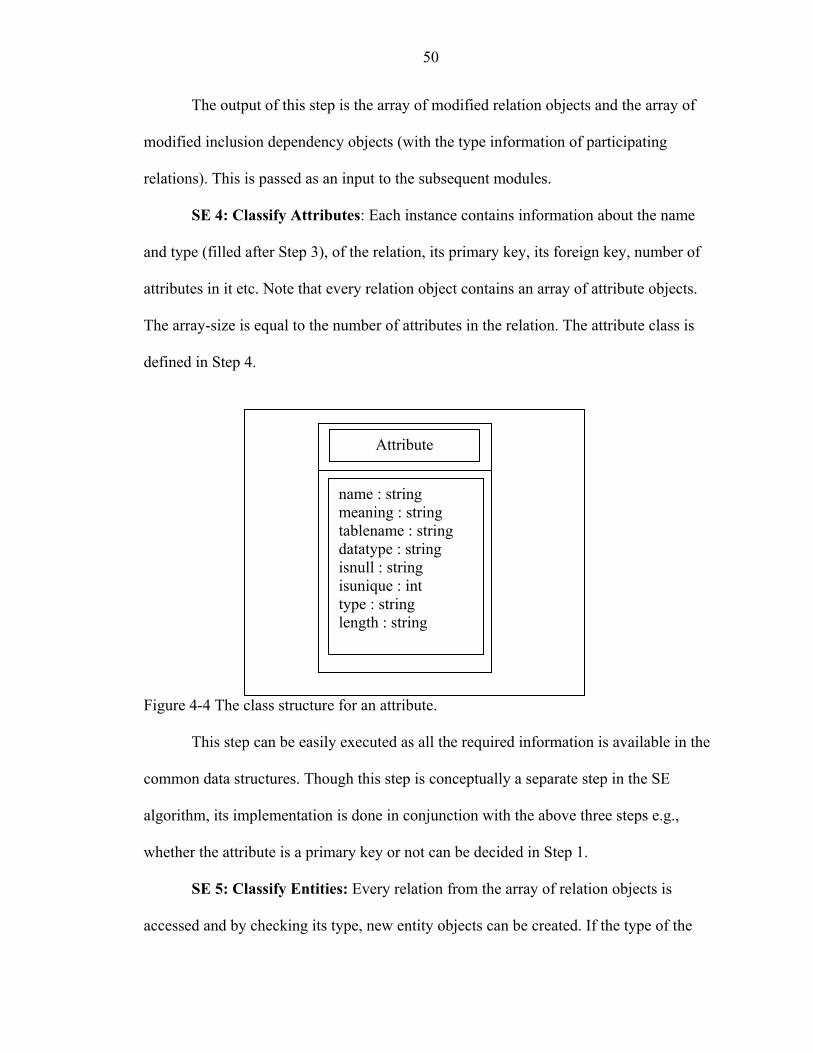
50
The output of this step is the array of modified relation objects and the array of
modified inclusion dependency objects (with the type information of participating
relations). This is passed as an input to the subsequent modules.
SE 4: Classify Attributes: Each instance contains information about the name
and type (filled after Step 3), of the relation, its primary key, its foreign key, number of
attributes in it etc. Note that every relation object contains an array of attribute objects.
The array-size is equal to the number of attributes in the relation. The attribute class is
defined in Step 4.
Figure 4-4 The class structure for an attribute.
name : string meaning : string tablename : string datatype : string isnull : string isunique : int type : string length : string
Attribute
This step can be easily executed as all the required information is available in the
common data structures. Though this step is conceptually a separate step in the SE
algorithm, its implementation is done in conjunction with the above three steps e.g.,
whether the attribute is a primary key or not can be decided in Step 1.
SE 5: Classify Entities: Every relation from the array of relation objects is
accessed and by checking its type, new entity objects can be created. If the type of the
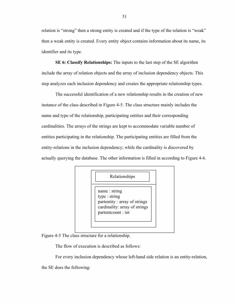
51
relation is “strong” then a strong entity is created and if the type of the relation is “weak”
then a weak entity is created. Every entity object contains information about its name, its
identifier and its type.
SE 6: Classify Relationships: The inputs to the last step of the SE algorithm
include the array of relation objects and the array of inclusion dependency objects. This
step analyzes each inclusion dependency and creates the appropriate relationship types.
The successful identification of a new relationship results in the creation of new
instance of the class described in Figure 4-5. The class structure mainly includes the
name and type of the relationship, participating entities and their corresponding
cardinalities. The arrays of the strings are kept to accommodate variable number of
entities participating in the relationship. The participating entities are filled from the
entity-relations in the inclusion dependency; while the cardinality is discovered by
actually querying the database. The other information is filled in according to Figure 4-6.
Figure 4-5 The class structure for a relationship.
name : string type : string partentity : array of stringscardinality: array of stringspartentcount : int
Relationships
The flow of execution is described as follows:
For every inclusion dependency whose left-hand side relation is an entity-relation,
the SE does the following:

52
1. If it is a strong entity with the primary key in the inclusion dependency, then an “is-a” relationship between two strong entities is identified.
2. If it is a strong entity with a non-primary key in the inclusion dependency, then “regular binary” relationship between two entities is identified.
3. If it is a weak entity with the primary key in an inclusion dependency, then a “dependent” or “has” relationship between two strong entities is identified.
4. If it is a weak entity with a non-primary key attribute in the inclusion dependency, then a “regular binary” relationship between two entities is identified.
For every inclusion dependency whose left hand side relation is a relationship-
relation, the SE does the following:
1. We know what relations are identified as regular and specific. We only have to identify the inclusion dependencies involving those primary keys (or subset of the primary keys) of these relations on the left-hand sides to find out the participating entities. The n-ary relationships, where n >2, are also identified similarly.
2. If we have a regular and specific relation with non-primary keys on the left-hand side, an “aggregate relationship” is identified.
Thus all the new relationships are created by analyzing the array of inclusion
dependencies. As a result, at the end of the schema extraction process, the output consists
of the array of relation objects, the array of entity objects and the array of relationship
objects.

53
Figure
encode
structur
(“result
informa
Consider an inclusion dependency: LHS-entity.LHS-attset << RHS-entity.RHS-attset 1. “IS-A” relationship:
Name: RHS-entity_is-a_LHS-entity Type: IS-A Cardinality: 1:1
2. Regular Binary relationship: Name: RHS-entity relates_to LHS-entity Type: Regular Binary Cardinality: 1:1/1:N (can be easily finalized by checking duplication)
3. “Dependent” or “has” Relationship Name: RHS-entity has LHS-entity Type: Dependent Cardinality: 1:N (with N at the weak entity side)
4. M:N Relationships Name: name of the corresponding relation Type: M:N Cardinality: M:N
5. Aggregate Relationship: Name: Aggregated-LHS-entity relates_to RHS-entity Type: Aggregate Cardinality: 1:1/1:N (can be easily finalized by checking duplication)
4-6 The information in different types of relationships instances.
Knowledge Encoder: When the schema extraction process is completed, the
r module is automatically called. This module has access to the common data
e. Using the extracted information, the encoder module creates an XML file
s.xml”) with proper formatting and conforms it to the predefined DTD. For more
tion about this DTD, please refer appendix A.

54
4.2 Example Walkthrough of Prototype Functionality
In this section, we present an exhaustive example of the Schema Extraction
process. We will also provide some screenshots of our working prototype. Project
management is a key application in the construction industry; hence the legacy source for
our example is based on a Microsoft Project application from our construction supply
chain testbed. For simplicity, we assume without loss of generality or specificity that
only the following relations exist in the MS-Project application, which will be discovered
using SE (for a description of the entire schema refer to Microsoft Project Website [42]):
MSP-Project, MSP-Availability, MSP-Resources, MSP-Tasks and MSP-Assignment.
Additionally, we also assume that the dictionary makes the following information
available to the SE algorithm namely relation and attribute names, all explicitly defined
constraints, primary keys (PKs), all unique constraints, and data types.
SE Step 1: Extracting Schema Information:
This step extracts the relation and the attribute names from the legacy source. A
decision step directs control to the semantic analyzer if the information about the primary
keys cannot be obtained from the dictionary.
Result: In the example DRE application, the following relations were obtained
from the MS-Project schema. Also all the attribute names, their data types, null
constraints and unique constraints were also extracted but are not shown to maintain
clarity.
MSP-Project [PROJ_ID, ...]
MSP-Availability[PROJ_ID, AVAIL_UID, ...]
MSP-Resources [PROJ_ID, RES_UID, ...]
MSP-Tasks [PROJ_ID, TASK_UID, ...]

55
MSP-Assignment [PROJ_ID, ASSN_UID, ...]
Figure 4-7 The screen snapshot describing the information about the relational schema.
Figure 4-7 presents a screen snapshot describing the information about the
relational schema including the relation names, attribute names, primary keys, simple
constraints etc. The reader can see a hierarchical structure describing a relational schema.
A subtree of the corresponding attributes is created for every relation in the relational
schema and all information is displayed when user clicks on the particular attribute. For
example, the reader can get information about the attribute TASK_FINISH_DATE (top
of the screen) including its datatype (datetime), meaning extracted from the code (Task
termination date), key information and simple constraints.
The hierarchical structure is chosen since it provides legibility, user-directed
display (as user can click on a relation name or attribute name for detailed information),
and ease of use. This structure is followed at all places in the user interface.

56
SE Step 2: Discovering Inclusion Dependencies.
This part of the DRE algorithm has two decision steps. First, all of the possible
inclusion dependencies are determined using SE. Then control is transferred to SA to
determine if there are equi-join queries embedded in the application (using pattern
matching against FROM and WHERE clauses). If so, the queries are extracted and
returned to SE where they are used to rule out erroneous dependencies. The second
decision determines if the set of inclusion dependencies is minimal. If so, control is
transferred to SE Step 3. Otherwise, the transitive dependencies are removed and the
minimal set of inclusion dependencies is finalized with the help of the user.
Result: Inclusion dependencies are listed as follows:
MSP_Assignment[Task_uid,Proj_ID] << MSP_Tasks [Task_uid,Proj_ID]
MSP_Assignment [Res_uid,Proj_ID] << MSP_Resources [Res_uid,Proj_ID]
MSP_Availability [Res_uid,Proj_ID] << MSP_Resources [Res_uid,Proj_ID]
MSP_Resources [Proj_ID] << MSP_Project [Proj_ID]
MSP_Tasks [Proj_ID] << MSP_Project [Proj_ID]
MSP_Assignment [Proj_ID] << MSP_Project [Proj_ID]
MSP_Availability [Proj_ID] << MSP_Project [Proj_ID]
The last two inclusion dependencies are removed on the basis of transitivity.
SE Step 3: Classification of the Relations.
Relations are classified by analyzing the primary keys obtained in Step 1 into one
of the four types: strong, weak, specific, or regular. If any unclassified relations remain,
then user input is requested for clarification. If we need to make distinctions between

57
weak and regular relations, then user input is requested, otherwise the control is
transferred to the next step.
Result:
Strong Entities: MSP_Project, MSP_Availability
Weak Entities: MSP_Resources, MSP_Tasks
Regular Relationship: MSP-Assignment
SE Step 4: Classification of the Attributes.
We classify attributes as (a) PK or FK, (b) Dangling or General, or (c) Non-Key
(if none of the above). Control is transferred to SA if FKs need to be validated.
Otherwise, control is transferred to SE Step 5.
Result: Table 4-1 illustrates attributes obtained from the example legacy source.
Table 4-1 Example of the attribute classification from the MS-Project legacy source.
PKA DKA FKA NKA
MS-Project Proj_ID
MS-Resources Proj_ID + Res_UID Res_UID
MS-Tasks Proj_ID +Task_UID Task_UID
MS- Availability Proj_ID +Avail_UID Avail_UID Res_UID+Proj_ID
MS-Assignment Proj_ID +Assn_UID Assn_UID Res_UID+ Proj_ID,
Task_UID+ Proj_ID
All
Remaining
Attributes
SE Step 5: Identify Entity Types.
In SE-5, strong (weak) entity relations obtained from SE-3 are directly converted
into strong (respective weak) entities.
Result: The following entities were classified:

58
Strong entities: MSP_Project with Proj_ID as its key.
MSP_Availability with Avail_uid as its key.
Weak entities: MSP_Tasks with Task_uid as key and MSP_Project as its owner.
MSP_Resources with Res_uid as key and MSP_Project as owner.
Figure 4-8 The screen snapshot describing the information about the entities.
Figure 4-8 presents the screen snapshots describing the identified entities. The
description includes the name and the type of the entity and also the corresponding
relation in the relational schema. For example the reader can see entity
MSP_AVAILABILITY (top of the screen), its identifier (AVAIL_UID) and its type
(strong entity). The corresponding relation MSP_AVAILABILITY and its attributes in
the relational schema can also be seen in the interface.
SE Step 6: Identify Relationship Types.
Result: We discovered 1:N binary relationships between the following entity
types:

59
Between MSP_Project and MSP_Tasks
Between MSP_Project and MSP_Resources
Between MSP_Resources and MSP_Availabilty
Since two inclusion dependencies involving MSP_Assignment exist (i.e., between
Task and Assignment and between Resource and Assignment), there is no need to define
a new entity. Thus, MSP_Assignment becomes an M:N relationship between
MSP_Tasks and MSP_Resources.
Figure 4-9 The screen snapshot describing the information about the relationships.
Figure 4-9 shows the user interface in which the user can view the information
about the identified relationships. After clicking on the name of the relationship, the user
can view the information such as its type, the participating entities and respective
cardinalities. The type of the relationship can be one of the types discussed in Step 6 of
DRE algorithm given in previous chapter. If the relationship is of M:N type, the
corresponding relation in the relational schema is also shown. For example, the reader
can see the information about the relationship MSP_ASSIGNMENTS in Figure 4-9. The

60
reader can see the type (M:N regular), participating entities (MSP_RESOURCES and
MSP_TASKS) and their corresponding cardinalities(M and N). The reader can also see
the corresponding relation MSP_ASSIGNMENTS.
Figure 4-10 E/R diagram representing the extracted schema.
The E/R diagram based on the extracted information shows four entities, their
attributes and relationships between the entities. Not all the attributes are shown for the
sake of legibility. MSP_Projects is a strong entity with Proj_ID as its identifier. The
entities MSP_Tasks and MSP_Resources are weak entities and depend on MSP_Projects.
Both weak entities participate in an M:N binary relationship MSP_Assignments.
MSP_Availability is also a strong entity participating in a regular binary relationship with
MSP_Resources. For the XML view of this information, the reader is referred to
APPENDIX B.

61
4.3 Configuration and User Intervention
As discussed earlier, the Adapter module needs to be modified for different
databases. These changes mainly include the name of the driver to connect to the
database, the procedure for making the connection, the method of providing the username
and password etc. Also, certain methods in the JDBC API might not work for all
relational databases because such compatibility is generally vendor dependent. Instead of
making all these changes every time or keeping different files for different databases, we
have provided command line input for specifying the database. Once the program gets the
name of the database (e.g., Oracle), it automatically configures the Adapter module and
continues execution automatically.
The next point of interaction with the user is before finalizing the inclusion
dependencies. If a set of final inclusion dependencies cannot be finalized without any
doubt, then that set is presented to the user with the corresponding rating as discussed in
the previous chapter. The user then selects the valid inclusion dependencies and rejects
the others. Though the user is guided by the rating system, he is not bound to follow that
system and may select any inclusion dependency if he is assured of its correctness. But
the result of this irregular manual selection cannot be predicted beforehand.
After the entire process is completed, the user can view the results in two forms.
The graphical user interface, automatically executed at the end of SE, shows complete
information in an easy and intuitive manner. Java Swing has been extensively used to
develop this interface. The other way to view the results is in the form of an XML
document generated by the knowledge encoder.
The sample XML representation of the extracted knowledge and its corresponding
DTD can be found in Appendix B and Appendix A respectively.

62
4.4 Integration
As discussed in the previous chapter, the integration of the Schema Extraction
algorithm with the Semantic Analysis results in the overall DRE algorithm. The design
and implementation of semantic analysis and code slicing is being done by another
member of our research group and hence has not been discussed in detail. Though the
main focus of this chapter is to present the implementation details of the schema
extraction process, we now provide brief insights on how the implementation takes care
of the interaction between SE and SA.
We have already listed the points where SE and SA interact. Initially, the
integrated prototype begins with the AST generation step of SA. This step then calls the
dictionary extractor. The notable change here is that the dictionary extractor no longer
contains the main method. Instead SA calls it as a normal method invocation. Similarly
SA calls the Analysis module (shown in Figure 4-1) after its code analysis phase.
One important point of interaction is in the dictionary extraction step. If enough
information about the primary keys is not found in the dictionary, the SE will pass a set
of candidate keys to SA in the form of an array. SA already has access to the query
templates that represent the predetermined patterns. SA operates on the AST to match
these patterns and takes decisions if the match is successful. The reduced set is then sent
back to SE as an array. We assume that we get strong clues about primary keys from the
dictionary and hence this interaction will rarely take place.
Another vital point of communication is the equi-join query finder. While
developing an integrated prototype, we have assumed that SE will simply invoke the
module and SA has the responsibility to find, shortlist and format these queries. SA will

63
send back inclusion dependencies in the inc_dependency object format discussed earlier.
Then SE takes over and completes the inclusion dependency detection process.
We have discussed the implementation issues in detail in this section and in the
previous section. The next section will conclude the chapter by providing the
implementation summary.
4.5 Implementation Summary
4.5.1 Features
Almost all the features of the SE algorithm discussed in Chapter 3 have been
implemented. The prototype can:
1. connect to the relational database via JDBC;
2. extract information about the underlying relational model with the help of our own small API built on the powerful JDBC API. This information includes relation names, column names, simple constraints, data types etc;
3. store that information in a common database like data structure;
4. infer possible inclusion dependencies and finalize the set of inclusion dependencies with the help of an expert user;
5. identify entities and the relationships among these entities;
6. present the extracted information to the user with an intuitive interface; as well as
7. encode and store the information in an XML document;
The prototype is built using the Java programming language. The JDBC API is
used to communicate with the database. The Java Swing API is used to generate all the
user interfaces. The choice of Java was motivated by its portability and robustness.
4.5.2 Advantages
The working prototype of the Schema Extraction also presents the following
notable advantages:

64
1. It minimizes user intervention and requests user assistance only at the most important step (if required).
2. The prototype is easily configurable to work with different relational databases.
3. The user interface is easy to use and intuitive.
4. The final XML file can be kept as a simple yet powerful form of documentation of the DRE process and can be used to guide the wrapper generation or any decision making process.
Though these are significant advantages, the main concern about prototype
implementation of the SE algorithm is its correctness. If the prototype does not give
accurate results, then having an elaborate interface or an easy configuration is of no
importance. The next chapter is dedicated to the experimental evaluation where we
present the results of testing this SE prototype.
We can conclude whether or not these advantages reflect positively in practical
scenarios or actual testing, only after the experimental evaluation of the prototype. Hence
the next chapter outlines the tests performed, discusses the experimental results, and
provides more insights about our working prototype.

CHAPTER 5 EXPERIMENTAL EVALUATION
Several parameters can be used to evaluate our prototype. The main criteria
include correctness or accuracy, performance, and ease of use. The schema extraction is
primarily a build-time process and hence is not time critical. Thus, performance analysis
based on the execution time is not an immediate issue for the SE prototype. The main
parameter in the experimental evaluation of our prototype is the correctness of the
information extracted by the prototype. If the extracted information is highly accurate in
diverse input conditions (e.g., less than 10% error), then the SE algorithm can be
considered useful. As SEEK attempts to be a highly automated tool for rapid wrapper re-
configuration, another important parameter is the amount of user intervention that is
needed to complete the DRE process.
We have implemented a fully functional SE prototype system, which is currently
installed and running in the Database Center at the University of Florida. We have run
several experiments in an effort to test our algorithm. We shall first give the setup on
which these experiments were conducted. In the next section, we shall explain the test
cases and the results obtained. Finally, we shall provide conclusive reasoning of the
results and summarize the experiments.
5.1 Experimental Setup
The DRE testbed resides on a Intel Pentium-IV PC with a 1.4 GHz processor, 256
MB of main memory, 512KB cache memory, running Windows NT. As discussed earlier,
all components of this prototype were implemented using Java (SDK 1.3) from Sun
65

66
Microsystems. Other tools used are the XML Parser from Oracle version 2.0.2.9, Project
scheduling software from Microsoft to prepare test-data, Oracle 8i RDBMS for storing
test-data and JDBC drivers from Sun and Oracle.
The SE prototype has been tested for two types of database systems; A MS-
Access/MS-Project database on the PC and an Oracle 8i database that is running on a
department’s Sun Enterprise 450 Model 2250 machine with 2 processors of 240MHz
each. The server has 640MB of main memory, 1.4GB of virtual memory and 2MB of
cache memory. This testbed reflects the distributed nature of business networks, in which
the legacy source and SEEK adapter will most likely execute on different hardware.
The DRE prototype connects to the database, either locally (e.g., MS-ACCESS)
or remotely (e.g., Oracle), using JDBC and extracts the required information and infers
the conceptual associations between the entities.
5.2 Experiments
In an effort to test our schema extraction algorithm, we selected nine different test
databases from different domains. The databases were created by graduate students as
part of a database course at the University of Florida. Each of these test cases contains
relational schema and actual data. The average number of tables per schema is
approximately 20 and the number of tuples ranges from 5 to over 50,000 per table. These
applications were developed for varied domains such as online stock exchange and
library management systems.
5.2.1 Evaluation of the Schema Extraction Algorithm
Each test database was used as an input to the schema extraction prototype. The
results were compared against the original design document to validate our approach. The
results are captured in Table 5-1.

67
Table 5-1 Experimental results of schema extraction on 9 sample databases.
Project Name Domain Phantom
INDs Missing
INDs Phantoms E/R Components
Missing E/R Components
Complexity Level
P1 Publisher 0 0 0+0 0+0 Low P9 Library 0 1 0+0 0+1 Low
P5 Online Company 0 0 0+0 0+0 Low
P3 Catering 0 0 0+0 0+0 Medium P6 Sports 0 0 0+0 0+0 Medium P4 Movie Set 1 0 0+1 0+0 Medium P8 Bank 1 0 0+1 0+0 Medium P7 Food 3 1 0+3 0+1 High
P2 Financial Transaction 5 0 0+5 0+0 High
The final column of Table 5-1 specifies the level of complexity for each schema.
At this point, all projects are classified into three levels based on our relational database
design experience. Projects P1, P9, P5 are given low complexity as the schema exhibited
meaningful and consistent naming systems; rich datatypes (total 11 different datatypes in
case of P9 and 17 in case of P1) relatively few relations (ranging from 10-15) with only
few tuples per relation (average 50-70 tuples per relation). A database having these
characteristics is considered a good database design and is richer in terms of semantic
information content. Hence for knowledge extraction process, these databases are more
tractable and should be rated with a low complexity level. Projects P3, P6, P8 and P2 are
less tractable than P1, P9 and P5 due to a limited number of datatypes (only 7 in case of
project P3), more relations (average 20 relations per schema) and more tuples per
relations than P1, P9 and P5. Project P7 and P2 have been rated most complex due to
their naming system and limited number of datatypes. For example in project P2, primary
key attribute of almost all tables are named as only ID. The importance of various factors

68
in complexity levels is better understood when the behavior and results of each schema
are studied. The details are given in Section 5.2.2.
Since the main parameter for evaluating our prototype is the “correctness of the
extracted information,” table 5-1 shows the errors detected in the experiments. These
errors essentially can be of two types, a missing concept (i.e., the concept is clearly
present but our SE algorithm did not extract it) or a phantom concept (i.e., the concept is
extracted by the SE algorithm but is absent in the data source). As the first step of the SE
algorithm merely extracts what is present in the dictionary, the errors only start
accumulating from the second step. The core part of the algorithm is inclusion
dependency detection. Steps 3, 4, 5, 6 use the final set of inclusion dependencies either to
classify the relations or to infer high-level relationships. Hence, an error in this step
almost always reflects as an error in the final result.
As previously discussed, when the decision about certain inclusion dependencies
cannot be finalized, the possible set is presented to the user with the appropriate rating
(low or high). In the experimental evaluation, we always assume that the user blindly
decides to keep the inclusion dependency with a high rating and rejects those with a low
rating. This assumption will help us reflect the exact behavior of SE algorithm, though in
real scenarios the accuracy can be increased by intelligent user decision. More details
about this are given in Section 5.3.2.
Thus omissions and phantoms have a slightly different meaning with respect to
our algorithm. Missing inclusion dependencies are in the set POSSIBLE that are ranked
low by our algorithm but do exist in reality; hence they are considered omissions.
Whereas phantom inclusion dependencies are in the set POSSIBLE that are ranked high
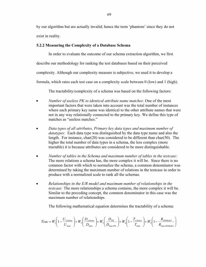
69
by our algorithm but are actually invalid; hence the term ‘phantom’ since they do not
exist in reality.
5.2.2 Measuring the Complexity of a Database Schema
In order to evaluate the outcome of our schema extraction algorithm, we first
describe our methodology for ranking the test databases based on their perceived
complexity. Although our complexity measure is subjective, we used it to develop a
formula, which rates each test case on a complexity scale between 0 (low) and 1 (high).
The tractability/complexity of a schema was based on the following factors:
•
•
•
•
Number of useless PK to identical attribute name matches: One of the most important factors that were taken into account was the total number of instances where each primary key name was identical to the other attribute names that were not in any way relationally connected to the primary key. We define this type of matches as “useless matches.”
Data types of all attributes, Primary key data types and maximum number of datatypes: Each data type was distinguished by the data type name and also the length. For instance, char(20) was considered to be different than char(50). The higher the total number of data types in a schema, the less complex (more tractable) it is because attributes are considered to be more distinguishable.
Number of tables in the Schema and maximum number of tables in the testcase: The more relations a schema has, the more complex it will be. Since there is no common factor with which to normalize the schema, a common denominator was determined by taking the maximum number of relations in the testcase in order to produce with a normalized scale to rank all the schemas.
Relationships in the E/R model and maximum number of relationships in the testcase: The more relationships a schema contains, the more complex it will be. Similar to the preceding concept, the common denominator in this case was the maximum number of relationships.
The following mathematical equation determines the tractability of a schema:
−+
−+
+
+
−=
ERModel
ERModelschema
PK
PKschemaschema
RR
WT
TW
DD
WD
DW
UU
WTracmax
5max
4max
3max
2max
1 111

70
Where U represents the useless name matches in a schema, U the
maximum number of useless name matches in all testcases, the number of
attribute data types in a schema, the maximum number of attribute data types in all
testcases, the number of primary key data types in a schema, the maximum
number of primary key data types in all testcases, T the number of tables in a
schema, the maximum number of tables in all testcases, the number of
relationships in the E/R model of a schema, and the maximum number of
relationships in the E/R models of all testcases. In addition, each factor was weighted to
indicate the importance of the factor with respect to the complexity of the schema.
schema max
PK
schemaD
ERModelR
maxD
PKD
maxT
Dmax
schema
ERModelmaxR
5.3 Conclusive Reasoning
The complexity measurement formula described in the previous section was used
to order the projects. Based on this ordering of the project, we plotted the results of Table
5-1 as two graphs to better illustrate the outcome of the experiments. The graphs are
shown in Figure 5-1. The graphs depict the errors encountered during inclusion
dependency detection and at the end of overall process.

71
Inclusion Dependency Results
0123456789
10
p1 p9 p5 p3 p6 p4 p8 p7 p2
Schemas (ascending complexity)
No. o
f pha
ntom
+ N
o of
mis
sing
In
ds No. of missing IndsNo of phantom Inds
E-R Results
0123456789
10
p1 p9 p5 p3 p6 p4 p8 p7 p2
Schemas (ascending complexity)
No o
f pha
ntom
+ N
o of
mis
sing
E-R
com
pone
nts No. of missing E-R
componentsNo. of phantom E-Rcomponents
Figure 5-1 Results of experimental evaluation of the schema extraction algorithm: errors in detected inclusion dependencies (top), number of errors in extracted schema (bottom). 5.3.1 Analysis of the Results
Both graphs in Figure 5-1 appear similar, since a phantom in an inclusion
dependency definitely results in a phantom relationship and a missing inclusion
dependency almost always results in a missing relationship. This is due to the fact that
every relationship is identified only from an inclusion dependency. After the set of
72
inclusion dependencies is finalized, every inclusion dependency in that set is used to
identify associations between participating entities. So, the presence of a phantom
inclusion dependency in the final set always indicates the presence of a phantom
relationship in the final result.
Phantoms are generated because some pairs of attributes in different tables are not
related even though they have name and datatype similarities and the subset relationship
holds. For example, consider two relations “Company” and “Person”. If both the relations
have an attribute called “ID” of integer type and if the subset relationship holds (due to
similar integer values or range), then the inclusion dependency “Company (ID) <<
Person (ID)” is definitely added to the POSSIBLE set. As there is a name similarity in
both the attributes, the SE algorithm will give a “high” rating to this inclusion
dependency while presenting it to the user. So if the user decides to keep it, a phantom
relationship between the concerned entities (Company and Person) will be identified in
the final result. The phantoms generally occur when the naming system in the database
design is not good (as shown by our example). It can also occur due to limited data values
or lack of a variety of datatypes in the schema. All of these contribute to the complexity
of the schema as discussed earlier.
Omissions occur because some pairs of attributes in different tables are actually
related even though they have completely unrelated and different names. For example,
consider two relations “Leaders” and “US-Presidents”. If the relation “Leader” has
attribute “Country#” and the relation “US-Presidents” has attribute “US #” and both the
attributes have integer datatype, then the subset relationship definitely holds. Since there
is no name similarity between the relations and the attributes, the SE algorithm will

73
attach a “low” rating to this inclusion dependency while presenting it to the user. If the
user rejects this possible inclusion dependency, a valid relationship between the
concerned entities (Leaders and US-Presidents) will be missing in the final result. Such
omissions generally occur when the naming system in the database design is inadequate
(as shown by our example).
Both the graphs in Figure 5-1 also suggest that there are comparatively fewer
omissions than phantoms. `The omissions will occur very rarely in our algorithm. This is
due to the fact that our exhaustive algorithm will miss something (i.e., give a low rating)
only when the tables and columns on both sides are completely unrelated in terms of
names. As this is very rare in normal database design, our algorithm will rarely miss
anything.
Another parameter for evaluation can be user intervention. The SE algorithm may
consult the user only at the inclusion dependency detection step. If the algorithm can not
finalize the set, it will ask the user to decide. This is a significant improvement over many
existing reverse engineering methods, although even this point of interaction might not be
necessary for well-designed databases.
5.3.2 Enhancing Accuracy
The accuracy discussions in the previous subsection are based on worst-case
scenarios. The main improvements can be done at the inclusion dependency detection
step, as it is the first step where errors start creeping in. As discussed earlier, the errors in
the final result are just the end-product of errors in this step. We shall now present simple
experiments that can be done to enhance the accuracy of the SE algorithm.
In the intermediate user intervention step, if the domain-expert makes intelligent
decisions about the existence of the possible inclusion dependencies ignoring the ratings,

74
the error rate can be decreased significantly. One additional experiment was to do exactly
this and the resulting error rate was almost zero in many of the above databases. Even if
the user is not a domain expert, some obvious decisions definitely enhance the accuracy.
For example, rejecting the inclusion dependency “Company (ID) << Person (ID)” even
though the corresponding rating is “high” is a common-sense decision and will certainly
reduce errors.
Another possible way to increase the correctness of the results is to use some kind
of a threshold. Sometimes the number of data values can be very different in two tables
and the subset relationship holds just by chance. This is mostly true when the data values
in the corresponding columns are integers or integer-ranges. For example, the “ID”
column in the relation “Task” may contain values 1 to 100, while the “ID” column in the
relation “Project” may contain values 1 and 2. This will lead to an invalid possible
inclusion dependency “Project (ID) << Task (ID)”. To reject these kinds of inclusion
dependencies, we can keep a dynamic threshold value. If the number of values in one
column dependent upon the number of values in the other column is less than the
threshold, then we can reject the dependency beforehand. Though this is helpful in many
cases, it can result in the rejection of some valid inclusion dependencies. The effect of
this improvement is not completely defined and the experiments did not show any
definite reduction of errors. But the procedure can be tweaked to get a reduced error rate
in majority of the cases.
In this section, we presented discussion of experimental results and the related
analysis. The results are highly accurate and have been obtained with minimum user
intervention. Accuracy can be further enhanced by simple additional methods. The next

75
section will summarize the main contributions of the schema extraction algorithm and
will provide valuable insights on the future enhancements at the algorithmic level. It will
also provide an overall summary of this thesis..

CHAPTER 6 CONCLUSION
Schema extraction and knowledge discovery from various database systems has
been an important and exciting topic of research for more than two decades now. Despite
all the efforts, a truly comprehensive solution for the database reverse engineering
problem is still elusive. Several proposals that approach this problem have been made
under the assumption that data sources are well known and understood. The substantial
work on this problem also remains theoretical, with very few implemented systems
present. Also, many authors suggest semi-automatic methods to identify database
contents, structures, relationships, and capabilities. However, there has been much less
work in the area of a fully automatic discovery of database properties.
The goal of this thesis is to provide a general solution for the database reverse
engineering problem. Our algorithm studies the data source using a call-level interface
and extracts information that is explicitly or implicitly present. This information is
documented and can be used for various purposes such as wrapper generation, forward
engineering, system documentation effort etc. We have manually tested our approach for
a number of scenarios and domains (including construction, manufacturing and health
care) to validate our knowledge extraction algorithm and to estimate how much user
input is required. The following section lists the contribution of this work and the last
section discusses possible future enhancements.
76

77
6.1 Contributions
The most important contributions of this work are the following. First, a broad
survey of existing database reverse engineering approaches was presented. This overview
not only updates us with the knowledge of the different approaches, but also provides a
significant guidance while developing our SE algorithm. The second major contribution
is the design and implementation of a relational database reverse engineering algorithm,
which puts minimum restrictions on the source, is as general as possible and extracts as
much information as it can from all available resources, with minimum external
intervention.
Third, a new and different approach to propose and finalize the set of inclusion
dependencies in the underlying database is presented. The fourth contribution is the idea
to use every available source for the knowledge extraction process. Giving importance to
the application code and the data instances is very vital. Finally, developing the formula
for measuring complexity of database schemas is also an important contribution. This
formula, which is based on the experimental results generated by our prototype, can be
utilized for similar purpose in various applications.
One of the more significant aspects of the prototype we have built is that it is
highly automatic and does not require human intervention except in one phase when the
user might be asked to finalize the set of inclusion dependencies. The system is also easy
to use and the results are well-documented.
Another vital feature is the choice of tools. The implementation is in Java, due to
its popularity and portability. The prototype uses XML (which has become the primary
standard for data storage and manipulation) as our main representation and
documentation language. Finally, though we have tested our approach only on Oracle,

78
MS-Access and MS-Project data sources, the prototype is general enough to work with
other relational data sources including Sybase, MS-SQL server and IBM DB2.
Though the experimental results of the SE prototype are highly encouraging and
its development in the context of wrapper generation and the knowledge extraction
module in SEEK is extremely valuable, there are some shortcomings of the current
approach. The process of knowledge extraction from databases can be enhanced with
some future work. The following subsection discusses some limitations of the current SE
algorithm and Section 6.3 presents possible future enhancements.
6.2 Limitations
6.2.1 Normal Form of the Input Database
Currently the SE prototype does not put any restriction on the normal form of the
input database. However, if it is in first or second normal form, some of the implicit
concepts might get extracted as composite objects. The SE algorithm does not fail on
2NF relations, but it does not explicitly discover all hidden relationships, although this
information is implicitly present in the form of attribute names and values. (e.g.,
cityname and citycode will be preserved as attributes of Employee relations in the
following example)
Consider following example:
Employee (SSN, name, cityname, citycode)
Project (ProjID, ProjName)
Assignment (SSN, ProjID, startdate)
In the relation Employee, the attribute citycode depends on the attribute cityname,
which is not a primary key. So there is a transitive dependency present in the relation and
hence it is in 2NF. Now if we run the SE algorithm over this schema, it first extracts table

79
names, attribute names as above. Then it finds the set of inclusion dependencies as
follows:
Assignment.SSN << Employee.SSN
Assignment.ProjID << Project.ProjID
The SE algorithm classifies relations (Employee and Project as strong relations
and Assignment as regular relation) and attributes. Finally it identifies Employee and
Project as strong entity and Assignment as M:N relationship between them. The
dependency of citycode on cityname is not identified as a separate relationship.
To explicitly extract all the objects and relationships, the schema should ideally
be in 3NF. This limitation can be removed by extracting functional dependencies (such as
citycode << cityname) from the schema and converting schema into 3NF before starting
the extraction process. Any kind of decision about normal form of legacy database is
difficult to make. One can not deduce easily whether the database is in 2NF or 3NF. Also
it may not be really useful for use to extract such extra relationships explicitly.
6.2.2 Meanings and Names for the Discovered Structures
Although the SE algorithm extracts all concepts (e.g entities, relationships)
modeled by the underlying relational database, it falls short in assigning proper semantic
meanings to some of the concepts. Semantic Analysis may provide important clues in this
regard but how useful they are depends largely on the quantity and quality of the code. It
is difficult to extract semantic meaning for every concept.
Consider an example. If the SE algorithm identifies a regular binary relationship
(1:N) between Resource and Availability, then it is difficult to provide meaningful name
to it. The SE algorithm gives the name “relates_to” in this case which is very general.

80
6.2.3 Adaptability to the Data Source
Ideally the algorithm should adapt successfully to the input database. However,
the accuracy of the results generated by the SE algorithm somewhat depends on quality
of database design, which includes proper naming system, richer datatypes and size of the
schema. The experimental results and the schema complexity measure discussed earlier
confirm this.
Although it is very difficult to attain high accuracy levels for broad range of
databases, the integration of SE algorithm with machine learning approaches might aid
the extraction process to achieve at least a minimal level of completeness and accuracy.
6.3 Future Work
6.3.1 Situational Knowledge Extraction
Many scheduling applications such as MS-Project or Primavera have a closed
interface. Business rules, constraints or formulae are generally not found in the code
written for these applications, since the application itself contain many rules. For
example, in the case of the MS-Project software, we can successfully access the
underlying database, which allows us to extract accurate but only limited information.
Our current schema extraction process (part of DRE) extracts knowledge about the
entities and relationships from the underlying database. Some additional but valuable
information can be extracted by inspecting the data values that are stored in the tuples of
each relation. This information can be used to influence decisions in the analysis module.
For example in the construction industry, the detection of a ‘float’ in the project schedule
might prompt rescheduling or stalling of activities. In warfare, the detection of the current
location and the number of infantry might prompt a change of plans on a particular front.

81
Since this knowledge is based on current data values, we call it situational
knowledge (sk). Situational knowledge is different from business rules or factual
knowledge because the deduction is based on current data that can be changed over the
time.
Some important points to consider:
•
•
•
1.
2.
3.
Extraction of sk has to be initiated and verified by a domain expert.
An ontology or generalization of terms must be available to guide this process.
The usefulness of this kind of knowledge is even greater in those cases where business rule mining from application source code is not possible.
It is also crucial to understand what sort of situational knowledge might be
extracted with respect to a particular application domain before thinking about the details
of the discovery process. This provides insights about the possible ways in which a
domain expert can query the discovery tool. This will also help the designer of the tool to
classify these queries and finalize the responses. We classify the sk in four broad
categories:
Situational Knowledge Explicitly Stored in the Database - Simple Lookup Knowledge: This type of sk can be easily extracted by one or more simple lookups and involves no calculation or computation. Extraction can be done through database queries. e.g., Who’s on that activity? (i.e., find the resource assigned to the activity) or what percentage of work on a particular activity has been completed?
Situational Knowledge Obtained through a Combination of Lookups and Computation: This type of sk extraction involves database lookups combined with computations (arithmetic operations). Some arithmetic operations (such as summation, average) can be predefined. The attribute names can be used as the parameters taking part in these operations. e.g., What is the summation of the durations of all activities in a project? Or what is the productivity of an activity as a function of the activity duration and units of resource assigned?
Situational Knowledge Obtained through a Comparison between two inputs: The request for a comparison between two terms can be made and the response will be in the form of two sets containing relevant information about these terms that can

82
be used to compare them. This may involve lookups and calculations. e.g., Compare the project duration and the sum of durations of all the activities in that project or compare the skill levels of resources working on different activities.
4.
•
•
•
•
Complex Situational Knowledge: This is the most complex type of sk extraction and can involve lookups, calculations and comparisons. For extracting this kind of knowledge, one has to provide a definite procedure or an algorithm. e.g., Find a float in the schedule, or find the overall project status and estimate the finish date.
As discussed above, the situational knowledge discovery process will be initiated
on a query from the domain expert, which assures a relatively constrained search on a
specific subset of the data. But the domain expert may not be conversant with the exact
nature of the underlying database including its schema or low-level primitive data. So,
the discovery tool should essentially consist of:
an intuitive GUI for an interactive and flexible discovery process.
the query transformation process.
the response finalizing and formatting process.
A simple yet robust user interface is very important in order to specify various parameters easily.
The process of query transformation essentially involves translation of high-level
concepts provided by the user to low-level primitive concepts used by the database. The
response finalizing process may involve answering the query in an intelligent way i.e., by
providing more information than was initially requested.
The architecture of the discovery system to extract situational knowledge from the
database will consist of the relational database, concept hierarchy, generalized rules,
query transformation and re-writing system and response finalization system. The
concept hierarchies can be prepared by organizing different levels of concepts into a
taxonomy or ontology. A concept hierarchy always related to specific attribute and is
partially ordered in general-to-specific order. The knowledge about these hierarchies

83
must be given by domain experts. Some researchers have also tried to generate or refine
this hierarchy semi-automatically [30], but that is beyond the scope of this thesis.
Generalization rules summarize the regularities of the data at a high level. As there are
usually a large set of rules extracted from any interesting subset, it is unrealistic to store
all of them. However it is important to store some rules based on frequency of inquiries.
The incoming queries can be classified as high-level or low-level based on the
names of its parameters. The queries can also be classified as data queries, which are
used to find concrete data stored in the database, or knowledge queries, which are used to
find rules or constraints. Furthermore, the response may include the exact answer, the
addition of some related attributes, information about some similar tuples, etc.
Such a discovery tool should be based on data mining methods. Data mining is
considered as one of the most important research topics in 1990s by both machine
learning and database researchers [56]. Various techniques have been developed for
knowledge discovery including generalization, clustering, data summarization, rule
discovery, query re-writing, deduction, associations, multi-layered databases etc. [6, 18,
29]. One intuitive generalization-based approach for intelligent query answering in
general and for situational knowledge in particular is based on a well-known data mining
technique called attribute-oriented induction in Han et al. [29]. This approach provides an
efficient way for the extraction of generalized data from the actual data by generalizing
the attributes in the task-relevant data-set and deducing certain situational conclusions
depending on the data values in those attributes.
The situational knowledge in SEEK can be considered as an additional layer to
the knowledge extracted by the DRE module. This kind of knowledge can be used to

84
guide the analysis module to take certain decisions; but it cannot be automatically
extracted without a domain expert.
This system may be integrated in SEEK as follows:
1. Create a large set of queries that are used on a regular basis to find the status in every application domain.
2. Create the concept hierarchy for the relevant data set.
3. After the DRE process, execute these queries and record all the responses.
4. The queries and their corresponding responses can be represented as simple strings or can be eventually added to general knowledge representation.
Appendix D describes detail example of the sk extraction process.
6.3.2 Improvements in the Algorithm
Currently our schema extraction algorithm does not put restriction on the normal
form of the input database. However, if the database is in 1NF or 2NF, then some of the
implicit concepts might get extracted as composite objects. To make schema extraction
more efficient and accurate, the SE algorithm can extract and study functional
dependencies. This will ensure that all the implicit structures can be extracted from the
database no matter what normalization form is used.
Another area of improvement is knowledge representation. It is important to
leverage existing technology or to develop our own model to represent the variety of
knowledge extracted in the process effectively. It will be especially interesting to study
the representation of business rules, constraints and arithmetic formulae.
Finally, although DRE is a build-time process, it will be interesting to conduct
performance analysis experiments especially for the large data sources and make the
prototype more efficient.

85
6.3.3 Schema Extraction from Other Data Sources
A significant enhancement would extend the SE prototype to include knowledge
extraction from multiple relational databases simultaneously or from completely non-
relational data sources. Non-relational database systems include the traditional network
database systems and the relatively newer object-oriented database systems. An
interesting topic of research would be to explore the extent to which, information can be
extracted without human intervention in such data sources. Also it will be useful to
develop the extraction process for distributed database systems on top of the existing
prototype.
6.3.4 Machine Learning
Finally, machine learning techniques can be employed to make the SE prototype
more adaptive. After some initial executions, the prototype could adjust its parameters to
extract more accurate information from a particular data source in a highly optimized and
efficient way. The method can integrate the machine learning paradigm [41], especially
learning from example techniques, to intelligently discover knowledge.

APPENDIX A DTD DESCRIBING EXTRACTED KNOWLEDGE
<?xml version="1.0"?>
<!DOCTYPE Model [
<!ELEMENT Database (Relational_Schema, Conceptual_Schema, Business_Rules)>
<!ELEMENT Relational_Schema (Relation+)>
<!ELEMENT Relation (Name, Type, Columns)>
<!ELEMENT Name (#PCDATA)>
<!ELEMENT Type (#PCDATA)>
<!ELEMENT Columns (Column+)>
<!ELEMENT Column (Name, DataType, Meaning, IsPK, FK, NullOption, IsUnique)>
<!ELEMENT Name (#PCDATA)>
<!ELEMENT DataType (#PCDATA)>
<!ELEMENT Meaning (#PCDATA)>
<!ELEMENT IsPK (#PCDATA)>
<!ELEMENT FK (IsFK, FKTable)>
<!ELEMENT IsFK (#PCDATA)>
<!ELEMENT FKTable (#PCDATA)>
<!ELEMENT NullOption (#PCDATA)>
<!ELEMENT IsUnique (#PCDATA)>
<!ELEMENT Conceptual_Schema (Entity+, Relationship+)>
<!ELEMENT Entity (Name, Type, Identifier)>
86

87
<!ELEMENT Name (#PCDATA)>
<!ELEMENT Type (#PCDATA)>
<!ELEMENT Identifier (#PCDATA)>
<!ELEMENT Relationship (Name, Type, Participants)>
<!ELEMENT Name (#PCDATA)>
<!ELEMENT Type (#PCDATA)>
<!ELEMENT Participants (Participant+)>
<!ELEMENT Participant (ParticipantEntity, Cardinality)>
<!ELEMENT ParticipantEntity (#PCDATA)>
<!ELEMENT Cardinality (#PCDATA)>
<!ELEMENT Business_Rules (Rule+)>
<!ELEMENT Rule (#PCDATA)>

APPENDIX B SNAPSHOTS OF “RESULTS.XML”
The knowledge extracted from the database is encoded into an XML document.
This resulting XML document contains information about every attribute of every
relation in the relational schema in addition to the conceptual schema and semantic
information. Therefore the resulting file is too long to be displayed completely in this
thesis. Instead, we provide snapshots of the document, which highlight the important
parts of the document.
Figure B-1 The main structure of the XML document conforming to the DTD in Appendix A.
Figure B-2 The part of the XML document which lists business rules extracted from the code.
88

89
Figure B-3 The part of the XML document which lists business rules extracted from the code.

90
Figure B-4 The part of the XML document, which describes the semantically rich E/R schema.

APPENDIX C SUBSET TEST FOR INCLUSION DEPENDENCY DETECTION
We are using the following subset test to determine whether there exists an
inclusion dependency between attribute (or attribute set) U of relation R1 and attribute
(or attribute set) V or R2. Note, U and V must have the same data type and must includes
the same number of attributes. Our test is based on the following SQL query templates,
which are instantiated for the relations and their attributes and are run against the legacy
source.
C1 = SELECT count (*) FROM R1 WHERE U not in (SELECT V FROM R2); C2 = SELECT count (*) FROM R2 WHERE V not in (SELECT U FROM R1);
Figure C-1 Two queries for the subset test.
If C1 is zero, we can deduce that there may exist an inclusion dependency R1.U
<< R2.V; likewise, if C2 is zero there may exist an inclusion dependency R2.V << R1.U.
Note that it is possible for both C1 and C2 to be zero. In that case, we can conclude that
the two sets of attributes U and V are equal.
91

APPENDIX D EXAMPLES OF THE SITUATIONAL KNOWLEDGE EXTRACTION PROCESS
Example 1:
Input: The table depicts a task-relevant subset of the relation “Assignment” in a database.
Resource Name Task Name Duration Units Cost
(days) ($) Tim’s crew Demolish Old Roof 2 1 3000
Tiles Install New Roof 0 1000 225 Brick Install New Roof 0 500 150
Barn’s crew Paint New Roof 10 1 5000 Cement Repair Wall covering 0 2000 500
Paint Painting 0 750 500 James’s crew Painting 2 1 2500 Tim’s crew Install New Roof 4 1 1500
Table No.1
Assume we already have the concept hierarchy as follows:
{Demolish Old Roof, Install New Roof, Paint New Roof} → Roofing
{Repair Wall covering, Painting} → Renovation
{Roofing, Renovation} → ANY (Task)
{Tim’s crew, Barn’s crew, James’s crew} → Labor
{Tiles, Bricks, Cement, Paint} → Material
{Labor, Material} → ANY (resources)
{1-100} → small
{101-1000} → medium
{>1000} → high
{small, medium, high} → ANY (Cost)
92

93
NOTE: A → B indicates that B is generalized concept of A.
Consider that a supervisor in this firm wants to check the resources assigned to
the roofing activities and the cost involved.
retrieve Resource Name and Cost
from Assignment
where Task Name = “Roofing”
This query can be translated using the concept hierarchy as follows:
select Resource Name, Cost
from Assignment
where Task Name= “Demolish Old Roof” or Task Name= “Install New Roof” or Task
Name = “Paint New Roof”
The response can be simple i.e., providing the names and the related costs of the
resources assigned to three tasks. The system may also provide an intelligent response. In
this case, the intelligent response might contain the corresponding durations or the
classification according to the type of resources. It might also contain information about
the resources assigned to another task such as Renovation.
Another query might be used to compare two things. For example,
compare
summation
{retrieve Duration
from Assignment
where Task Name = Roofing
}

94
with
retrieve Duration
from Project
where Project Name = House#11
This query will result in 2 queries to the database. First query will find out the
duration for the repairs of the house number 11. Second query will find total duration of
the roofing related activities in the database. This will involve adding summing durations
from each row of the result-set. The response will enable the user to take important
decisions about the status of roofing with respect to entire project.
NOTE:
The general format for high-level queries used above can be manipulated and
finalized by taking into account all the possible queries. For more information the reader
is referred to [28].
The relation names and attribute names in a high-level query can be taken from
the domain ontology. These names should not necessarily be the same as their names in
the database. In a query translation process, these names can be substituted with actual
names from the mappings. Some of the mappings are found by the semantic analysis
process, while some mapping can be given by domain expert.
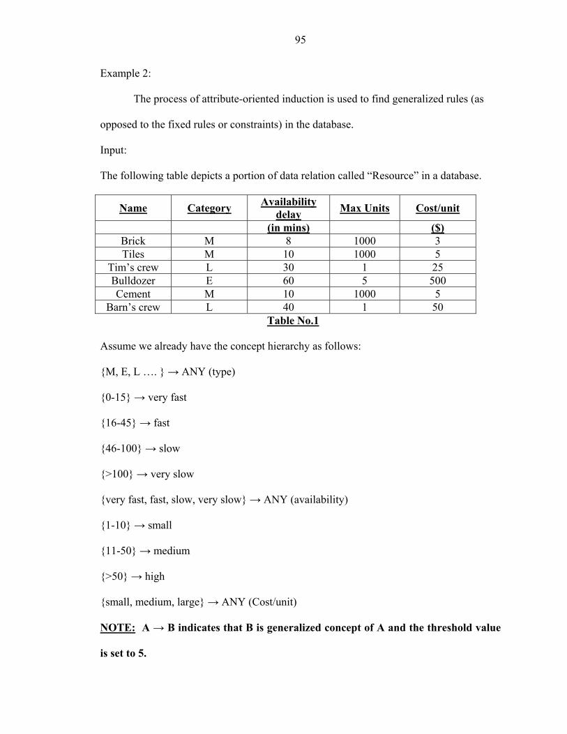
95
Example 2:
The process of attribute-oriented induction is used to find generalized rules (as
opposed to the fixed rules or constraints) in the database.
Input:
The following table depicts a portion of data relation called “Resource” in a database.
Name Category Availability delay Max Units Cost/unit
(in mins) ($) Brick M 8 1000 3 Tiles M 10 1000 5
Tim’s crew L 30 1 25 Bulldozer E 60 5 500 Cement M 10 1000 5
Barn’s crew L 40 1 50 Table No.1
Assume we already have the concept hierarchy as follows:
{M, E, L …. } → ANY (type)
{0-15} → very fast
{16-45} → fast
{46-100} → slow
{>100} → very slow
{very fast, fast, slow, very slow} → ANY (availability)
{1-10} → small
{11-50} → medium
{>50} → high
{small, medium, large} → ANY (Cost/unit)
NOTE: A → B indicates that B is generalized concept of A and the threshold value
is set to 5.

96
The query can be -
describe generalized rule
from Resource
about Name and Category and Availability Time and Cost .
General Methodology:
1. Generalize on the smallest decomposable components of a data relation. A special attribute “vote” is added to every table initially and its value is kept 1 for every tuple. The vote of tuple t represents the number of tuples in the initial data relation generalized to tuple t of the current relation.
2. If there is large set of distinct values for an attribute, but there is no high level concept for the attribute, then that attribute should be removed.
3. Generalize the concept one level at a time. Removal of redundant tuples is carried out with addition of votes.
4. If the number of tuples of the target class in the final generalized relation exceeds the threshold, further generalization should be performed.
5. Transform rules to CNF and DNF. However, Step 6 should be performed to add quantitative information in the rule.
6. The vote value of a tuple should be carried to its generalized tuple and the vote should be accumulated in the preserved tuples when other identical tuples are removed. The rule with the vote value is presented to the user. The vote value gives the percentage of total records or tuples in the database that represents the same rule. This is typically used for presenting a quantitative rule
Example:
1. We first remove attribute max units as the expected generalized rule doesn’t take that attribute into account.
2. If there is large set of distinct values for an attribute, but there is no high level concept for the attribute, it should be removed. Thus, the “Name” attribute is removed.

97
Category Availability time Cost/unit Vote
M 8 3 1 M 10 5 1 L 30 25 1 E 60 500 1 M 10 5 1 L 40 50 1
Table No.2
3. Generalize the concept one level at a time – Doing this step multiple times will give the following table:
Category Availability time Cost/unit Vote
M Very fast Small 1 M Very fast Small 1 L Fast Medium 1 E Slow High 1 M Very fast Small 1 L Fast Medium 1
Table No.3
Removal of redundant tuples yields the following table:
Category Availability time Cost/unit Vote
M Very fast Small 3 L Fast Medium 2 E Slow High 1
Table No.4
5.
6.
If the number of tuples of the target class in the final generalized relation exceeds the threshold, further generalization should be performed - Removal of redundant tuples should result in a lesser number of tuples than the threshold. We have kept our threshold as 5 and there are no more than five tuples here, so no generalization is required.
The value of the vote for a given tuple should be carried to its generalized tuple and the vote should be accumulated in the preserved tuples when other identical tuples are removed The initial vote values are shown in the table no. 2. When we generalize and remove the redundant tuples the final vote values are shown in the table no. 4

98
7. Present the rule to the user. One of the final rules can be given in English as follows “Among all the resources in the firm 50% are materials whose availability time is very fast and their cost is smallest …”

LIST OF REFERENCES
[1] P. Aiken, Data Reverse Engineering: Slaying the Legacy Dragon, McGraw-Hill, New York, NY, 1997.
[2] N. Ashish, and C. Knoblock, “Wrapper Generation for Semi-structured Internet Sources,” Proc. Int’l Workshop on Management of Semistructured Data, ACM Press, New York, NY, pp. 160-169, 1997.
[3] G. Ballard and G. Howell, “Shielding Production: An Essential Step in Production
Control,” Journal of Construction Engineering and Management, ASCE, vol. 124, no. 1, pp. 11-17, 1997.
[4] R. Bayardo, W. Bohrer, R. Brice, A. Cichocki, G. Fowler, A. Helal, V. Kashyap,
T. Ksiezyk, G. Martin, M. Nodine, M. Rashid, M. Rusinkiewicz, R. Shea, C. Unnikrishnan, A. Unruh, and D. Woelk, “Semantic Integration of Information in Open and Dynamic Environments,” Proc. SIGMOD Int’l Conf., ACM Press, New York, pp. 195-206, 1997.
[5] D. Boulanger and S. T. March, “An Approach to Analyzing the Information
Content of Existing Databases,” Database, vol. 20, no. 2, pp. 1-8, 1989. [6] R. Brachman and T. Anand, The Process of KDD: A Human Centered Approach,
AAAI/MIT Press, Menlo Park, CA, 1996. [7] M. E. Califf, and R. J. Mooney, “Relational Learning of Pattern-match Rules for
Information Extraction,” Proc. AAAI Symposium on Applying Machine Learning to Discourse Processing, AAAI Press, Menlo Park, CA, pp. 9-15, 1998.
[8] M. A. Casanova and J. E. A. d. Sa, “Designing Entity-Relationship Schemas for
Conventional Information Systems,” Proc. Int’l Conf. Entity-Relationship Approach, C. G. Davis, S. Jajodia, P. A. Ng, and R. T. Yeh, North-Holland, Anaheim, CA, pp. 265-277, 1983.
[9] R. H. L. Chiang, “A Knowledge-based System for Performing Reverse
Engineering of Relational Database,” Decision Support Systems, vol. 13, pp. 295-312, 1995.
[10] R. H. L. Chiang, T. M. Barron, and V. C. Storey, “Reverse engineering of
Relational Databases: Extraction of an EER Model from a Relational Database,” Data and Knowledge Engineering, vol. 12, pp. 107-142, 1994.
99
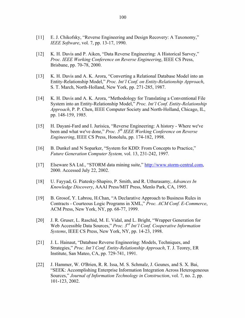
100
[11] E. J. Chikofsky, “Reverse Engineering and Design Recovery: A Taxonomy,”
IEEE Software, vol. 7, pp. 13-17, 1990. [12] K. H. Davis and P. Aiken, “Data Reverse Engineering: A Historical Survey,”
Proc. IEEE Working Conference on Reverse Engineering, IEEE CS Press, Brisbane, pp. 70-78, 2000.
[13] K. H. Davis and A. K. Arora, “Converting a Relational Database Model into an
Entity-Relationship Model,” Proc. Int’l Conf. on Entity-Relationship Approach, S. T. March, North-Holland, New York, pp. 271-285, 1987.
[14] K. H. Davis and A. K. Arora, “Methodology for Translating a Conventional File
System into an Entity-Relationship Model,” Proc. Int’l Conf. Entity-Relationship Approach, P. P. Chen, IEEE Computer Society and North-Holland, Chicago, IL, pp. 148-159, 1985.
[15] H. Dayani-Fard and I. Jurisica, “Reverse Engineering: A history - Where we've
been and what we've done,” Proc. 5th IEEE Working Conference on Reverse Engineering, IEEE CS Press, Honolulu, pp. 174-182, 1998.
[16] B. Dunkel and N Soparker, “System for KDD: From Concepts to Practice,”
Future Generation Computer System, vol. 13, 231-242, 1997. [17] Elseware SA Ltd., “STORM data mining suite,” http://www.storm-central.com,
2000. Accessed July 22, 2002. [18] U. Fayyad, G. Piatesky-Shapiro, P. Smith, and R. Uthurasamy, Advances In
Knowledge Discovery, AAAI Press/MIT Press, Menlo Park, CA, 1995. [19] B. Grosof, Y. Labrou, H.Chan, “A Declarative Approach to Business Rules in
Contracts - Courteous Logic Programs in XML,” Proc. ACM Conf. E-Commerce, ACM Press, New York, NY, pp. 68-77, 1999.
[20] J. R. Gruser, L. Raschid, M. E. Vidal, and L. Bright, “Wrapper Generation for
Web Accessible Data Sources,” Proc. 3rd Int’l Conf. Cooperative Information Systems, IEEE CS Press, New York, NY, pp. 14-23, 1998.
[21] J. L. Hainaut, “Database Reverse Engineering: Models, Techniques, and
Strategies,” Proc. Int’l Conf. Entity-Relationship Approach, T. J. Teorey, ER Institute, San Mateo, CA, pp. 729-741, 1991.
[22] J. Hammer, W. O'Brien, R. R. Issa, M. S. Schmalz, J. Geunes, and S. X. Bai,
“SEEK: Accomplishing Enterprise Information Integration Across Heterogeneous Sources,” Journal of Information Technology in Construction, vol. 7, no. 2, pp. 101-123, 2002.

101
[23] J. Hammer, M. Schmalz, W. O’Brien, S. Shekar, and N. Haldavnekar, “SEEKing
Knowledge in Legacy Information Systems to Support Interoperability,” CISE Technical Report, CISE TR02-008, University of Florida, 2002.
[24] J. Hammer, M. Schmalz, W. O’Brien, S. Shekar, and N. Haldavnekar, “SEEKing
Knowledge in Legacy Information Systems to Support Interoperability,” Proc. Int’l Workshop on Ontologies and Semantic Interoperability, AAAI Press, Lyon, pp. 67 –74, 2002.
[25] J. Hammer, H. Garcia-Molina, J. Cho, R. Aranha, and A. Crespo, “Extracting
Semistructured Information from the Web,” Proc. Int’l Workshop Management of Semistructured Data, ACM Press, New York, NY, pp. 18-25, 1997.
[26] J. Hammer, H. Garcia-Molina, Y. Papakonstantinou, J. Ullman, and J. Widom,
“Integrating and Accessing Heterogeneous Information Sources in TSIMMIS,” Proc. AAAI Symposium on Information Gathering, AAAI Press, Stanford, CA, pp. 61-64, 1995.
[27] J. Han, J. Chiang, S. Chee, J. Chen, Q. Chen, S. Cheng, W. Gong, M. Kamber, K.
Koperski, G. Liu, Y. Lu, N. Stefanovic, L. Winstone, B. Xia, O. R. Zaiane, S. Zhang, and H. Zhu, “DBMiner: A System for Data Mining in Relational Databases and Data Warehouses,” Proc. Int'l Conf. Data Mining and Knowledge Discovery, AAAI Press, Newport Beach, CA, pp. 250-255, 1997.
[28] J. Han, Y. Huang, N. Cercone, and Y. Fu, “Intelligent Query Answering by
Knowledge Discovery Techniques,” IEEE Transactions on Knowledge and Data Engineering, vol. 8, no. 3, pp. 373-390, 1996.
[29] J. Han, Y. Cai and N. Cercone, “Data-Driven Discovery of Quantitative Rules in
Relational Databases,” IEEE Transactions on Knowledge and Data Engineering, vol. 5, no. 1, pp. 29-40, 1993.
[30] J. Han and Y. Fu, “Dynamic Generation and Refinement of Concept Hierarchies
for Knowledge Discovery in Databases,” Proc. AAAI Workshop on Knowledge Discovery in Databases (KDD'94), AAAI Press, Seattle, WA, pp. 157-168, 1994.
[31] J. Hensley and K. H. Davis, “Gaining Domain Knowledge while Data Reverse
Engineering: An Experience Report,” Proc. Data Reverse Engineering Workshop, Euro Reengineering Forum, IEEE CS Press, Brisbane, pp. 100-105, 2000.
[32] S. Horwitz and T. Reps, “The Use of Program Dependence Graphs in Software
Engineering,” Proc. 14th Int’l Conf. Software Engineering, ACM Press, New York, NY, pp. 392-411, 1992.

102
[33] L. P. Jesus and P. Sousa, “Selection of Reverse Engineering Methods for Relational Databases", Proc. Int’l Conf. Software Maintenance and Reengineering, ACM Press, New York, NY, pp. 194-197, 1999.
[34] P. Johannesson, “A Method for Transforming Relational Schemas into
Conceptual Schemas,” Proc. IEEE Int’l Conf. Data Engineering, ACM Press, New York, NY, pp. 190-201, 1994.
[35] M. Kamber, L. Winstone, W. Gong, S. Cheng, and J. Han, “Generalization and
Decision Tree Induction: Efficient Classification in Data Mining,” Proc. Int’l Workshop Research Issues on Data Engineering (RIDE), IEEE CS Press, Birmingham, pp. 111-120, 1997.
[36] C. Klug, “Entity-Relationship Views over Uninterpreted Enterprise Schemas,”
Proc. Int’l Conf. Entity-Relationship Approach, P. P. Chen, North-Holland, Los Angeles, CA, pp. 39-60, 1979.
[37] L. Koskela and R. Vrijhoef, “Roles of Supply Chain Management in
Construction,” Proc. 7th Annual Int’l Conf. Group for Lean Construction, U.C. Press, Berkley, CA, pp. 133-146, 1999.
[38] J. Larson and A. Sheth, “Federated Database Systems for Managing Distributed,
Heterogeneous, and Autonomous Databases,” ACM Computing Surveys, vol. 22, no. 3, pp. 183-236, 1991.
[39] V. M. Markowitz and J. A. Makowsky, “Identifying Extended Entity-Relationship
Object Structures in Relational Schemas,” IEEE Transactions on Software Engineering, vol. 16, pp. 777-790, 1990.
[40] M. A. Melkanoff and C. Zaniolo, “Decomposition of Relations and Synthesis of
Entity-Relationship Diagrams,” Proc. Int’l Conf. Entity-Relationship Approach, P. P. Chen, North-Holland, Los Angeles, CA, pp. 277-294, 1979.
[41] R. S. Michalski, Machine Learning: An Artificial Intelligence Approach, Morgan
Kaufmann Publishers, San Mateo, CA, 1986. [42] Microsoft Corp., “Microsoft Project 2000 Database Design Diagram,”
http://www.microsoft.com/office/project/prk/2000/Download/VisioHTM/P9_dbd_frame.htm, 2000. Accessed August 15, 2001.
[43] C. H. Moh, E. P. Lim, and W. K. Ng, “Re-engineering Structures from Web
Documents,” Proc. ACM Int’l Conf. Digital Libraries, ACM Press, New York, NY, pp. 58-71, 2000.

103
[44] P. Muntz, P. Aiken, and R. Richards, “DoD Legacy Systems: Reverse Engineering Data Requirements,” Communications of the ACM, vol. 37, pp. 26-41, 1994.
[45] S. B. Navathe, C. Batini, and S. Ceri, Conceptual Database Design – An Entity
Relationship Approach, Benjamin-Cummings Publishing Co., Redwood City, CA, 1992.
[46] S. Nestorov, J. Hammer, M. Breunig, H. Garcia-Molina, V. Vassalos, and R.
Yerneni, “Template-Based Wrappers in the TSIMMIS System,” ACM SIGMOD Int’l. Conf. on Management of Data, ACM Press, New York, NY, pp. 532-535, 1997.
[47] W. O'Brien, M. A. Fischer, and J. V. Jucker, “An Economic View of Project
Coordination,” Journal of Construction Management and Economics, vol. 13, no. 5, pp. 393-400, 1995.
[48] Oracle Corp., “Data mining suite (formerly Darwin),”
http://technet.oracle.com/products/datamining/listing.htm. Accessed July 22, 2002.
[49] Y. Papakonstantinou, A. Gupta, H. Garcia-Molina, and J. Ullman, “A Query
Translation Scheme for Rapid Implementation of Wrappers,” Proc. 4th Int’l Conf. Deductive and Object-Oriented Databases, T. W. Ling, A. O. Mendelzon, and L. Vieille, Lecture Notes in Computer Science, Springer Press, Singapore, pp. 55-62, 1995.
[50] S. Paul and A. Prakash, “A Framework for Source Code Search Using Program
Patterns,” Software Engineering Journal, vol. 20, pp. 463-475, 1994. [51] J. M. Petit, F. Toumani, J. F. Boulicaut, and J. Kouloumdjian, “Towards the
Reverse Engineering of Denormalized Relational Databases,” Proc Int’l Conf. Data Engineering, ACM Press, New York, NY, pp. 218-229, 1996.
[52] W.J. Premerlani, M. Blaha, “An Approach for Reverse Engineering of Relational
Databases,” CACM, vol. 37, no. 5, pp. 42-49, 1994. [53] Sahuguet, and F. Azavant, “W4F: a WysiWyg Web Wrapper Factory,”
http://db.cis.upenn.edu/DL/wapi.pdf, Penn Database Research Group Technical Report, University of Pennsylvania, 1998. Accessed September 21, 2001.
[54] J. Shao and C. Pound, “Reverse Engineering Business Rules from Legacy
System,” BT Journal, vol. 17, no. 4, pp. 179-186, 1999.

104
[55] O. Signore, M. Loffredo, M. Gregori, and M. Cima, “Using Procedural Patterns in Abstracting Relational Schemata,” Proc. IEEE 3rd Workshop on Program Comprehension, IEEE CS Press, Washington D.C., pp. 169-176, 1994.
[56] M. StoneBreaker, R.Agrawal, U.Dayal, E. Neuhold and A. Reuter, “DBMS
Research at Crossroads: The Vienna update,” Proc. 19th Int’l Conf. Very Large Data Bases, R. Agrawal, S. Baker, and D. A. Bell, Morgan Kaufmann, Dublin, pp. 688-692, 1993.
[57] Sun Microsystems Corp., “JDBC Data Access API: Drivers,”
http://industry.java.sun.com/products/jdbc/drivers. Accessed January 10, 2002. [58] D. S. Weld, N. Kushmerick, and R. B. Doorenbos, “Wrapper Induction for
Information Extraction,” Proc. Int’l Joint Conf. Artificial Intelligence (IJCAI), AAAI Press, Nagoya, vol. 1, pp. 729-737, 1997.
[59] T. Wiggerts, H. Bosma, and E. Fielt, “Scenarios for the Identification of Objects
in Legacy Systems,” Proc. 4th IEEE Working Conference on Reverse Engineering, I. D. Baxter, A. Quilici, and C. Verhoef, IEEE CS Press, Amsterdam, pp. 24-32, 1997.
[60] World Wide Web Consortium, “eXtensible Markup Language (XML),”
http://www.w3c.org/XML/, 1997. Accessed March 19, 2001. [61] World Wide Web Consortium, “Resource Description Framework,”
http://www.w3c.org/RDF/, 2000. Accessed March 21, 2002. [62] World Wide Web Consortium, “Semantic Web,” http://www.w3.org/2001/sw/,
2001. Accessed October 19, 2001. [63] World Wide Web Consortium, “W3C Math Home,” http://www.w3c.org/Math/,
2001. Accessed March 21, 2002. [64] M.J. Zaki, S. Parthasarathy, M. Ogihara, and W. Li, “New algorithms for Fast
Discovery of Association Rules,” Proc. Intl. Conf. Knowledge Discovery and Data Mining, AAAI Press, Newport Beach, CA, pp. 283-286, 1997.

BIOGRAPHICAL SKETCH
Nikhil Haldavnekar was born on January 2, 1979, in Mumbai (Bombay), India.
He received his Bachelor of Engineering degree in computer science from VES Institute
of Technology, affiliated with Mumbai University, India, in August 2000.
He joined the department of Computer and Information Science and Engineering
at the University of Florida in fall 2000. He worked as a research assistant under Dr.
Joachim Hammer and was a member of Database Systems Research and Development
Center. He received a Certificate of Achievement for Outstanding Academic
Accomplishment from the University of Florida. He completed his Master of Science
degree in computer engineering at the University of Florida, Gainesville, in December
2002.
His research interests include database systems, Internet technologies and mobile
computing.
105


