An Adjacency Algorithm for Cylindrical Algebraic ... · An Adjacency Algorithm 165 Such cylindrical...

J. Symbolic Computation (1988) 5, 163-187

An Adjacency Algorithm for Cylindrical Algebraic Decompositions of

Three-dimenslonal Space*

DENNIS S. ARNON, GEORGE E. COLLINS*

AND SCOTT McCALLUM*

Xeroz PARC, 3333 Coyote Hill Road, Palo Alto, California 9~30~, U.S.A. Department of Computer and Information Sciencej The Ohio State University, Columbus,

Ohio ~3~i0 U.S.A. $ Research School of Physical Science, Australian National University, Canberra ACT ~601,

Australia

(Received 20 April 1985, and in revised form 15 November 1987)

Let A C Z [31, • . . , mr] be a finite set. An A-innarlan~ cylindrical algebraic decomposition (cad) is a certain partition of r-dimenslonal euclidean space E r into semi-algebraic cells such that the value of each Ai E A has constant sign (positive, negative, or zero) throughout each cell. Two cells are adjacent if their union is connected. We give an algo- r i thm that determines the adjacent pairs of cells as it constructs a cad of E 3. The general teehnlque employed for E 3 adjacency determination is "projection" into E 2, followed by application of an existing E 2 adjacency elgorlthm (Arnon, Collins, McCallum, 1984). Our algorithm has the following properties: (1) it requires no coordinate changes, end (2) in any cad of E 1 , E 2, or E a that it builds, the boundary of each cell is a (disjoint) union of lower-dlmenaionel cells.

1 I n t r o d u c t i o n

In this p a p e r we give a n a l g o r i t hm which de te rmines the pairs of a d j a c e n t cells as i t c o n s t r u c t s a c y l i n d r i c a l a lgebra ic decompos i t ion (cad) of t h r e e - d i m e n s i o n a l euc l idean space E z. O u r a l g o r i t h m is an ex tens ion to E a of the work o f A r n o n eL al. (1984b) , where we gave a n a l g o r i t h m t h a t de termines the pairs o f a d j a c e n t cells as it c o n s t r u c t s a cad o f t h e p l a n e E z.

We b e g i n by f o r m a l i z i n g some no t ions re la t ing to cell b o u n d a r i e s in cad ' s ( the reader may wish to refer to A r n o n eL al., 1984a, 1984b, for t e rmino logy tha t we do no t redef ine here). R e c a l l t h a t we cal l a connec ted subset of E T, r > 1 a region, and we say t h a t the boundary of a r eg ion X C E T, wr i t t en cgX, is the set of all l imi t poin ts of X n o t in X . It is n o t h a r d to see t h a t two d is jo in t regions are ad jacen t if a n d only if one c o n t a i n s

*This work was supported by the National Science Foundation (Grant MCS-8009357 to the Unlversity of Wlsconsln-Madison), the Purdue Research Foundation, and the Xerox Corporation. This paper was typeset at Xerox PARC using TF_,X in the Cedar environment.

0747-1717/88/010163+25 $03.00/0 © 1988 Academic Press Limited

164 D.S. Arnon et al.

a boundary point of the other. We say that a cad D of E ~, has the boundary properly if (1) for each cell c of D, Oc is the union of (zero or more) lower dimensional cells of D, and (2) if r > 2, then the induced cad D ' of E "-1 has the boundary property. It is not hard to see that the following is an equivalent s ta tement of (1): if ceils c and d of D are adjacent , then they have different dimensions, and the smaller-dimensional cell is contained in the boundary of the larger-dimensional cell. It is easy to see that any cad of E 1 has the boundary property. The cad's of E 2 that the algorithms we give in this paper "~ill build are proper in the sense defined by Arnon et el. (1984]~). From the fact that any cad of E ~ has the boundary property, and Corollary 2.5 of Arnon et el. (1984b), if follows that any proper cad of E 2 has the boundary property. It is a prerequisite for the E a adjacency algorithms that we give in this paper that the induced cad of E 2 have the boundary property.

Let D be a cad of E ~, v > 2. Recall tha t D consists of stacks over the cells of D' , the induced cad of E ~-1, and that for any cell c E D I, S(c) denotes the unique stack over c which is par t of D. We say tha t stacks S(c) and S(d) of D are adjacent if {c, d} is an adjacency of D I. If D ~ has the boundary property, then clearly any pair of adjacent stacks of D have different dimensions (the dimension of a stack is defined to be the dimension of its sectors), cells of the larger-dimensional stack have boundary points in (cells of) the smaller-dimensional stack, and no cell of the smaller-dimensional stack has any boundary points in (cells of) the larger-dimensional stack. Indeed, if D ~ has the boundary property~ then it is not hard to see that given any stack S(c) of D, and any element s of S(c), then all boundary points of s lle in (certain cells of) S(c) and in (certain cells of) the stacks S(d), where d ranges over all cells in ac. In other words, each boundary point of s is either in the same stack as s, or in some adjacent, lower-dimensional stack. Hence all cells of D that are adjacent to s either belong to the same stack as s, or are contained in some adjacent, lower-dimenslonal stack.

The considerations of the above paragraph give us our s t rategy for cad and adjacency construction in EZ: we build a certain cad D of E a such tha t the induced cad D t of E ~ has the boundary proper ty 3 then for each adjacency ~c, d} of D t, we find all interstack adjaeencies among the cells of S(c) and S(d) (interstack adjacencies are those in which the two ce.lls involved belong to different stacks). As always, it is trivial to determine the intrastack adjacencies of D (intrastack adjacencies are those in which the two cells involved belong to the same stack). Clearly if a cad of E 2 has the boundary property, then the possible multisets of dimensions of a pair of adjacent cells in it are {1, 2}, {0, 1}, and {0, 2}. Let us be sure that this notation is clear: the multiset {0, 1}, for example, refers to an adjacent pair of cells where one is a 0-cell and the other a 1-cell.

Given a set of r-variate polynomials A C I, -- Z [$~ , . . . , u , ] , a set X in E "-1 is nullifying (for A) if some Ai • A is nullified on X, i.e. A, (a, z~) -- 0 for all a in X. Previous papers have used the terms "AI is identically zero on X " (Arnon et al, 1984a) and "Ai vanishes identically on X" (McCallum, 1988) as synonyms for "Ai is nullified on X" . The essential point of the notion of a proper cad of E 2 is that no cell of the induced cad of the line nullifies the defining polynomial of the cad of E 2. For cad's of E a, as we will show in Section 2, we must in general change coordinates in order to have a t r ivar iate defining polynomial for the cad that is not nullified by any cell of the induced cad of the plane. The algorithm we present in this paper for constructing cad's of E s does not change coordinates. One reason for this is tha t if we change coordinates, construct a cad, and then return to the original coordinate system, the cells of the decomposition are no longer arranged into cylinders with respect to the original coordinate system.

An Adjacency Algorithm 165

Such cylindrical arrangement of cells, with respect to the original coordinate system, is crucial to the use of cad's for quantifier elimination (see Collins, 1975). It is possible to p u t ex t ra cells into the decomposition so that it is cylindrical with respect to two coord ina te systems, but this seems likely to be expensive.

I t is the case (see Section 2) that for the cad's of three space that our algorithm const ruc ts , any nullifying cell in the induced cad of the plane is 0-dimensional. Such nullifying 0-cells have the interesting property of permitting choice in the exact makeup of the s tack in E z that is constructed over them. Consider, for example / ; ( ~ , y , z ) = ~z -- y. I f we are constructing an F-invariant cad of E a, the point < 0, 0 > will be a nullifying 0-cell in the induced cad of the plane. Any stack over it is F-invariant, so the quest ion arises - does it mat ter what stack we choose to use as part of our F-invariant cad o f E37 The answer is yes. We will specify precisely how the stacks over nullifying 0-cells are to be constructed. The requirements we impose yield cad's of E a which have the b o u n d a r y property.

T h a t our cad's of E z have the boundary property is useful for two reasons. First, as was the case in Arnon et al. (1984b), it implies that there is a certain proper subset of i n t e r s t ack adjacencies (essentially, the so-caUed "section-section" adjacencies), which, once found, allow us to infer all other interstack adjacencies. Second, it helps us to ac tua l ly find the adjacencies of this sufficient subset, by guaranteeing us that when we p e r f o r m certain "projections" of an •3 adjacency situation into E 2 (e.g. slicing by a ce r ta in plane, or computing a certain resultant), the adjaceneies we then see in E 2 have a defini te correspondence with the actual adjaceneies present in E a, and we can "read off" the E 3 adjacencies from the E 2 data. Sections 3-6 amplify and substantiate these p re l imina ry remarks.

Altogether , we will distinguish four categories ofadjacencies in the (induced) cad's of E 2 t h a t we build: {1, 2}, {0, 1}, nonnullifying {0, 2} (i.e. a {0, 2} adjacency in which the 0-cell is nonnullifying), and nullifying {0, 2} (i.e. a {0, 2} adjacency in which the 0-cell is nullifying). In Sections 3-6 we consider each of these cases individually. Algorithm S S A D J 3 of Section 4 is the key subalgorithm for E s adjacency determination: a method for reducing an E a adjacency determination to an E 2 determination that we can do wi th algori thm SSADJ2 of Arnon et al. (1984b). In Section 7 we summarize previous sect ions with a main algorithm (called CADA3) that constructs a cad of/i~ a and its adjacencies , and we complete the proof that a cad of E a contructed by CADA3 has the b o u n d a r y property. Section 8 traces CADA3 on an example. We have not yet done extens ive study of our implementation of CADA3, but typically the cost of adjacency de t e rmina t ion seems not to exceed the cost of cad construction. The examples considered in A r n o n (1988) provide further data on CADA3's behavior in practice.

In Arnon et al. (1984b) we constructed proper cad's of E 2. In the present paper we cons t ruc t basis -de termined cads of E a (definition given in Section 2). A cad of E 2 is p r o p e r if and only ff it is basis-determined, however for euclidean space of dimension th ree or more, the notion of basis-determined cad is slightly more general. In Section 2 we prove the sameness of the two notions for E 2 (which allows us to use the results and a l g o r i t h m s of Arnon et al., 1984b), and explain the need for basis-determined cad's of E a"

A t the time the work reported in this paper was carried out (1979-1981), the prior work on incidence or adjacency algorithms that we knew of was tha t of McCa lhm (1979) for t r iangulat ion of real algebraic curves and surfaces, and our own adjacency algorithm for cad ' s of the plane (Arnon et. al., 1984b). It was also known that adjacency of cells

166 D: S. At'non et al.

in a cad of E ' , for any r, is decidable (Arnon, 1979). Subsequent to our work, other cad adjacency algorithms have been given (Prill, 1986; Kozen & Yap, 1985; Schwartz & Shark, 1983). These algorithms can be used for cad 's of E ~ for any 7', a n d avoid nullifying cells in the induced cad by changing coordinates. We are not aware t h a t any of them has been implemented.

2 Basis-determlned cylindrical algebraic decompositions

We say that the sign of an element o f I 0 is its sign as an integer, and tha t for r > 1, the sign of an element of I, = I,-1(~,), is the sign of its leading coefficient, an e lement of I t - 1. An element F of I, is positive if sign(E) is posi t ive.

Recall that for any F E I, -= I,_1(~,), the conten~ of F, wri t ten con~en~(F), is the greatest common divisor of F ' s coefficients. We adopt the conven t ion that sign(eon$enL(F)) is chosen to be sign(E). Any F for which con~en~(F) -= -_kl is said to be pr4mi~ive. The primiLive par~ of F, written pp(F), is F/eon$en$(F). Hence i f F ~ 0, then pp(F) is primitive and positive. We define cor~en~(O) --- 1 and pp(O) -~ O. Also, again viewing I , as I ,_l(z ,) , we define the degree of F E I , , written deg(F), to be its degree in z , . If we are interested in the degree of F w i t h respect to some o ther variable zi, we shall say "degree of F in zi".

B C I~ is a basis if each element of B is primitive, positive, and of pos i t ive degree, and if the elements of B are pairwise relatively prime. Let A C I t . A basis B C I~ is a basis for A if (1) For each A~ E A that is of positive degree, there exist (not necessari ly

k B distinct) B ~ , . . . , Bk E B, k > 1, such that Ai = con~en~(A~) I-Ij-~ 3 , and (2) Each Bi E B divides some A~ E A_Recall that for any F E ! , , V(F) de~otes the real var iety o f F , i.e. the set of all real zeros o f F , a subse t o r e r . A cad D o f E ' , r > 1, is basis- determined if there exists a basis B C I , such that (1) D is B-invariant, (2) every section of D is contained in V(F) for some F E B, and (3) i f r > 1, then D' is bas i s -de te rmined . We say that B is a basis for D.

THEOKEM 2.1 A cad of E 2 is basis-determined if and only if it is proper (in the sense of Arnon et al., 198~b).

PROOF, Suppose D is a proper cad of E ~, with defining polynomial _P'. Since V(F) is equal to the union of the sections of D, F is not t h e zero polynomial, and V ( F ) = V(pp(F)). Without loss of generality we may assume tha t F is also of pos i t ive degree (if not, then we may multiply it by y2 + 1). Thus {pp(F)} is a basis. Clear ly D is pp(F)-invariant, and every section of D is contained in V(pp(F)). If G E /1 is a defining polynomial for D' , then G is not the zero polynomial, V(G) -- Y(pp(G)), {pp(G)} is a basis, it is easy to see that {pp(G~} is a basis for D I, hence D ~ is basis-determined~ and so by Theorem 2.1 ofArnon et al. (1984b), D is basis-determined.

Suppose D is a basis-determined cad of E 2, with basis B. Let B I be a basis for D I. Set F -- I1 B, and G = ~ B~; both F and G are pr imit ive. It is clear tha t V ( G ) is the union of all the sections o l d ~, and from the fact that F is primitive it follows t h a t V(F) is the union of all the sections of D. Hence D is p roper []

It follows immediately from the next theorem tha t in a basis-deterrfiined cad of E3, any nullifying cell in the induced cad of E 2 is a 0-cell.


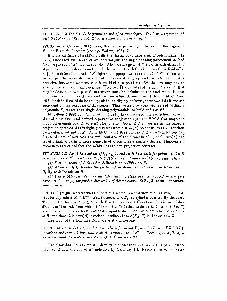
THEOREM 2.2 Let F ~ I3 be primitive and of positive degree. Let R be a region in E 2 such that F is nullified on R. Then R consists of a single point.

PROOF. As McCallum (1988) notes, this can be proved by induction on the degree of F using Bezout's Theorem (see e.g. Walker, 1978). D

It is the existence of nullifying cells that forces us to have a set of polynomials (the basis) associated with a cad of E a, and not just the single defining polynomial we had for a proper cad of E 2. Let us see why. When we are given A C I2~ with each element of A primitive, then it doesn' t mat ter whether we work with the elements of A individually, or I-[ A, to determine a cad of E 2 (given an appropriate induced cad of El); either way we will get the same A-invariant cad. However if A C h , and each element of A is primitive, but some element of A is nullified at a point p E E z, then we may not be able to construct our cad using just I I A. For I-[ A is nullified on p, but some F E A may be delineable over p, and its sections must be included in the stack we build over p in order to obtain an A-invariant cad (see either Arnon et al., 1984a, or McCallum, 1988, for definitions of delineability; although slightly differen L these two definitions are equivalent for the purposes of this paper). Thus we have to work with sets of "defining polynomials", rather than single defining polynomials, to build cad's of E a.

McCallum (1988) and Arnon ei al. (1984a) have discussed the projection phase of the cad algorithm, and defined a particular projection operator PT~OJ that maps the input polynomials A C Ir to P R O J ( A ) C I t-1. Given A C I , , we use in this paper a projection operator that is slightly different from P R O J ( A ) , to construct an A-invariant basis-determined cad of E ' . As in MeCallum (1988), for any A C I,, r >_ 1, let coni(A) denote the set of non-zero non-unit contents of the elements of A~ and pr im(A) the set of primitive parts of those elements of A which have positive degree. Theorem 2.3 introduces and establishes the validity of our new projection operator.

THEOREM 2.3 Let A be a subset of Ir, r > 2, and let B be a basis f o rpr im(A) . Let R be a region in E ~-t which is both PROJ(B)- invar iant and cong(A)-invariant. Then

( i) Every element of B is either delineable or nullified on R. (2) Where BR E I~ denotes the product of all elements of B which are deIineable on

R, BR is delineable on R. (3) Where S(BR, R) denotes the (B-invariant) stock over R induced by Bn (see

Arnon et al., 1984a, for further discussion of this notation), S( BR, R) is an A-invariant stock over R.

PROOF. (1) is just a restatement of part of Theorem 3.4 ofArnon et al. (1984a). Recall that for any subset X C E ~-1, Z ( X ) denotes X x E, the cylinder over X. By the same Theorem 3.4, for any F, G E B, each F-section and each G-section of Z(R) are either disjoint or identical, from which it follows that BR is delineable on R. Clearly S(BR, R) is B-invariant. Since each element of A is equal to its content times a product of elements of B, and since R is cont(A)-invariant, it follows that S(BR, R) is A-invariant. o

The proof of the following Corollary is straightforward.

COROLLARY 2.4 Let A C It, let B be a basis for pr im(A) , and let D' be a P R O J ( B ) - invariant and eont( A )-invariant basis-determined cad of E r-1 . Then Oce o, S ( Bc, c) is on A-invariant, basis-determined cad of E" (with basis B ).

The algorithm CADA3 we will develop in subsequent sections of this paper essentially constructs the cad of E 8 indicated by Corollary 2.4. However, as we indicated

I68 D.S. Amon et aL

in Section 1, the adjacency algorithms we develop in Sect ions 3-6 require tha t CADA3 put additional sections in the stacks over nullifying 0-cells in the plane (it is easy to see that after doing so, we still have an A-invariant, basis-determined cad of E3). Fig. 2 gives the actual algorithm E~tendCellToStack that we use for cad extension; it calls algorithm CellE~tensionPolynomial given in Fig. 1. At th i s point we have no t fully motivated all the particulars of these two algorithms, but s u c h motivat ion will be given by the end of Section 6.

Let us now define certain notations and terms used in these and subsequen t algorithms. Throughout this and subsequent sections we f ree ly use the var iables ~ ,y , z interchangably with ~1, ~2, z3. For F E/3 , let F~, Fu, and F~ denote the par t ia l deriva- tives of F w i t h respect t o z , y, a n d z . Let F a n d G b e e lements o f /3 . I f bo th F and G have positive degree in y, then Resu(F, G) denotes the resul tant of F and G with respect to y (see Walker (1978) for the definition of resu l tan t ) . If only one of F and G has positive degree in y, say F, then Resu(F, G) denotes G ( ~ , 0, z). I f nei ther F nor G has positive degree in y, then Resu(F, G)is undefined. Res,(F, G) and Resz(F,G) are defined similarly. We say that a polynomial f(w), with coefficients in any unique factorization domain, is squarefree if it has no multiple fac tors . The greatest square free divisor of f , written gsfd(f), is defined to be f divided b y gcd(f, f'). It is easy to see that gsfd(f) is a squarefree polynomial whose roots a r e the same as those of f . Kaltofen (1982) and Collins & Loos (1982) discuss squarefree factorization a lgor i thms. We use the phrase i-section (i-sector) as a shorthand for " /-dimensional cell which is a section (sector) in some cad". When an algorithm has a "cel l" as an input (e.g. input c of algorithm CellE~.tensionPolynomial), it is assumed t h a t the index, and a sample point, for that cell are provided in any actual call to the a lgor i thm.

3 Adjacencies over a {1, 2} a d j a c e n c y in t h e p l a n e

Let S be a stack. Recall from Arnon et al. (1984b) that S* , the extension o f S, is S together with two infinite sections (at positive and nega t ive infinity). Also, we may speak of the underlying cylinder of S, written Zs, which is jus t the union of (the e l emen t s of) S. Zs*, the extension of Zs, is Zs together with two infini te sections. G iven two adjacent stacks S and T in E', r :> 2, we say that S* has t h e unique section boundary property (USBP) in T* if for any section s of S*, the b o u n d a r y points of s in Z~.* constitute a section t of T* such that dimension(t) < dimension(s). T h e o r e m 2.2 of Arnon et al. (1984b) establishes that in a proper cad of the plane, any 2-stack has the USBP in each of the two 1-stacks adjacent to it, and so shows us how to d e t e r m i n e all section-section adjacencies in a (proper) cad of the plane. "Sect ion-sect ion" adjeLcencies are those in which both of the cells involved are sections of t he i r respective s tacks .

Theorem 2.3 of Arnon et al. (1984b) showed us how to infer all interstack adjacencies between two adjacent stacks of a proper cad of the plane, from knowledge of their sec t ion- section interstack adjacencies. The proof of Theorem 2.3 is easily generalized to show that in a cad of r-space, r > 2, if S* has the USBP in a s t a c k T*, then the b o u n d a r y of any sector of S in ZT.* is an "interval" [u, v] of ZT*, such tha t u and v are sec t ions of T* (this interval notation is from Arnon eL al., 1984b), . Thus in a cad of r - s p a c e , r > 2, when one stack has the USBP in another, de terminat ion of the sec t ion-sec t ion interstack adjacencies between the two stacks suffices for de te rmina t ion of all i n t e r s t a c k adjacencies between them.


g ~- C e l l ] E x t e n s l o n P o l y n o m l a l (c, B ~, B)

Inputs: c i s a c e l l i n a basis-determined cad D t o f E ~-1, r >_ 2. B' C Ir-~ is a b a s i s for D I. B C I~ is a basis, such that each element of B is either delineable or nullified on c.

Outputs: Let p = < pl,...,P~.-1 > be the sample point for c, and suppose the real algebraic number -y is a pr imit ive element for p, i.e. each Pl ~ Q(7). g is a non~.ero squarefree univariate polynomial g(z~) with coefficients in the field Q(*/), and whose real roots are in one-one correspondence with the sections of a B-invariant stack S over c.

(1) [Get initial g, check for null ifying 0-cell in E2.] Initialize the set F to be {B~(p~, ...,p~_~, ~ ) } . I f c i s a 0-cell in E ~ that nullifies some element of B (i.e. r = 3 and Be ¢ I-IB), then go to step (2), else go to step (3).

(2) [Add more factors of g if nullifying 0-cell in E ~.] Let B~v be the se~ of elements of B that are nullified on c, i.e. the elements of B that c nullifies. For each F E Br¢~ do the following steps (2.1)- (2.3):

(2.1) [Possible boundary 0-sections in S*(c) of V(F) over sections of D ' adjacent to c.] Set B(~,v) e ~ to be l-I ~" Set C(~, ~) e Z~ to be p~,(ges~(~,F)). Add a(p~, ~) to r.

(2.2) [Possible boundary 0-sections in S*(c) of V(F) over sectors of D ' adjacent to c.] Let M(z) C I~ be the min ima l polynomial of p~. Set G(y,z) e 12 to be pp(Res®(M,F)). Add G(p2,z) to F.

(2.3) [Possible boundary 0-sectlons in S*(c) of V(_~) over interior sections of part ial derivative projections (cf. Section 6).] For each element T(~,y) of the set { pp(Res,(F,F~)), pp(Res,(Y,F,)) }, do the following loop: if T of positive degree in y, and if T(p~,p2) = O, then set a ( ~ , ~ ) , - p p ( n e ~ ( T , F ) ) , a,d add a(p~,~)to r.

(3) [~ake a.] g(*,) ' - a~Yd([I r). o

Figure 1: A l g o r i t h m Ce l lEz~ens ionPo lynomia l .

E x t e n d C e l l T o S t a c k (c, B ~, B; g, J, I , L)

Inputs: c i s a c e l l i n a bas is -de tcrminedcad D ~ o f E r - l ~ r > 2. B ~ C I t -1 i s a b a s i s for D ~, B C I~ is a basis, such that each element of B is either detineable or nullified on c.

Outputs: Let p be the sample point for c~ and suppose the real algebraic number 7 is a primitive element for p (see Arnon et aI. (1984a) for this terminology), g is a nonzero univar ia te polynomial g(z~) with coemcients in the field Q(7), and whose real roots are in one-one correspondence with the sections of a B-invariant stack S over c. J is a list of isolating intervals for the real roots of g. ] is a list of ceil indices for the elements of S (cell indices are defined in Section 4 of Arnon et al., 1984a). L is a list of the intrastack adjacencies of S.

(1) [Get g, isolate roots, make up outputs.] g(~,) *-- CellEztensionPolynomial(c,B',B). Isolate the real roots of g to get J . Assuming we know the cell index of c~ then once we know how many real roots g has, we know the indices for the cells that comprise S, and so it is easy to make up I and Z. D

Figure 2: A lgor i thm Ex tendCe l lToS tack .


We now establish that in a basis-determined cad of E 3, we h a v e the U S B P over a {1, 2} adjacency in the induced cad of the plane.

THEOREM 3.1 Let D be a basis-determined cad orE 3. Let {c 1, c ~} be a {1, 2} adjacency olD'. Then S*(e ~) has the unique section boundary property in S * ( e l ) .

PROOF. If s is an infinite section of S*(c2), then Os ~g*(e 1) is the c o r r e s p o n d i n g infinite section of S*(c~). Suppose that s is a finite section of S*(c2), and t h a t it has a finite boundary point p in Z(cl) . Let B C I , be a basis for D. There is s o m e F E B such that s C V(F), and since V(F) is closed, p E V(F). By Theorem 2.2, F d o e s n ' t vanish on Z(et) , hence by the F-invariance of S(c~), p lies on a section t of S ( c l ) , a n d t C V(F). We claim there is a relative open ball U of p in t, such tha~ U C Ds. S u p p o s e to the contrary that for every open ball U of p in t, there exists q E U s u c h t h a t q ~ Os. For any such q, q = < cr,~ >, a E c 1, ~ E E, s has a l imi t point r E Z* ( ~ ) . Since r E V(F),

lies on a section u of S* (cl). Suppose tha t s is an f-section, for a c o n t i n u o u s funct ion f : c ~ --+ E. As the radius of U goes to 0, by the continuity o f f , 7' a p p r o a c h e s p. But then u and t intersect at p, a contradiction. Hence for any finite b o u n d a r y p o i n t p of s in Z(c~), lying on section ~ of S(c~), there is a relative open ball U o f P in ~ such ~hat U COs. If there exists a point q E ~ which is not in Os, then clear ly the re is a relative open ball of q in t which is disjoint from Os. Hence ~ can be s e p a r a t e d in to disjoint nonempty open (in the relative topology on g) subsets, cont rad ic t ing its connec tedness . Hence if s has a finite boundary point in g(cl), then there is a f in i t e sec t ion o f S(e ~) contained in Os, and clearly tha t is all of Os A Z*(cl). If s has no f in i te b o u n d a r y points in Z(c~), then it is not difficult to see tha t Os N Z*(e ~) is an infinite sec t ion of Z*(c~). Obviously ~ has dimension one and s has dimension two, i.e. t is of l o w e r d imens ion . []

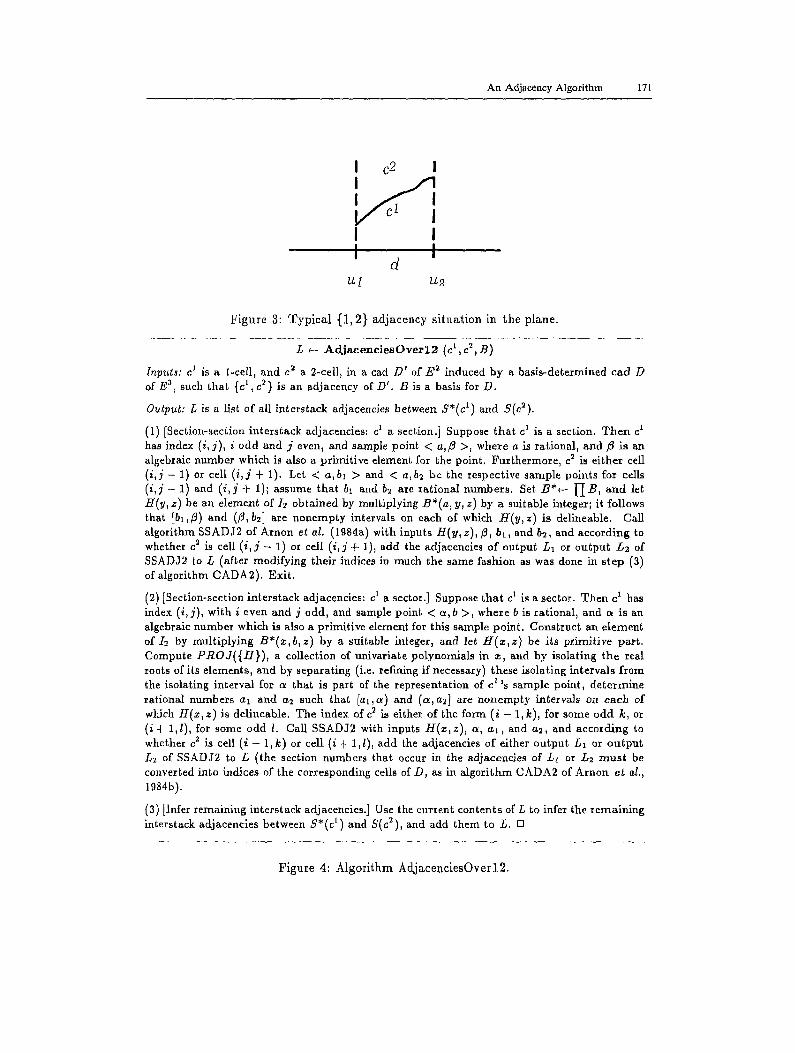
We now sketch an algorithm for determining the section-section ad j acenc i e s over a {1, 2} adjacency {c~,c ~} of a basls-determined cad D ' of E 2. S u p p o s e first t h a t c 1 is a section of D' , with c ~ C V(G) for some G(z, y) E B', where B ' is a bas i s for D ' . Then there exists a 1-cell d i n the induced cad orE 1, such that c 1 C Z(d), a n d c 2 is the sector of g(d) either immediately above or immediately below c 1. d is an o p e n in terva l , say (ul, u2). Fig. 3 illustrates the way things might look in the zy-plane. O u r s t r a t e g y is to pick some rational a E (ul, u2) and take a two-dimensional "slice" o f the c a d o f E a by the plane z = a. We then apply algori thm SSADJ2 o f A r n o n et al. ( 1 9 8 4 b ) to de t e rmine the adjaceneies present in the slicing plane, between the "slices" o f t he two s tacks of interest. The USBP we established in Theorem 3.1 guarantees us t h a t r ega rd less o f wha t particular a E (ul, u2) we pick, we will see the same adjacencies in the slicing p lane , and that the adjacencies we see there are in one-one correspondence with t h e ad jacene ie s in E a. If e 1 is a sector, then it has the form {~} x (v~, v2), for real a l geb ra i c n u m b e r s ~, v~, and v2, such that a -- c o is a 0-cell in the induced cad of El . We p r o c e e d in a fash ion entirely analogous to the section case, picking a rational b E (vl, v2), a n d sl icing by the plane y = b. The complete algorithm is given in Fig. 4.

4 AdSacencies over a {0, 1} adjacency in t h e p l a n e

In this section, we introduce the main idea of subalgori thm SSADJ3 wi th an example , prove a theorem to establish the general validity of this idea, and c o n c l u d e wi th our algorithm for determination of interstaek adjacencies over a {0, 1} a d j a c e n c y in the plane. At the outset, it appears tha t the cases of a nonnullifying {0, 1} a d j a c e n c y and


I C2 I I I I

I I I I

d ~I lz2

Figu re 3: T y p i c a l {1, 2} ad j acency s i t u a t i o n in the p lane .

L ~--- A d j a e e n c l e s O v e r l 2 (c l, e ~, B)

Inputs: c j is a 1-cell, and c z a 2-cell~ in a cad D ~ of E 2 induced by a bas is-determined cad D o f E ~, such that {cl,c 2 } is an adjacency o f D ' , B is a basis for D.

Output: L is a list of all in ters tack adjacencies between S*(c 1) and S(c2).

(1) [Section-section in te rs tack adjacencies: c 1 a section.] Suppose t h a t e 1 is a section. T h e n c ~ has index (i,j), i odd and j even, and sample point < a,/3 >, wheze a is ra t ional , and 13 is an algebraic number which is also a pr imit ive element for the point. Fur thermore , c 2 is ei ther cell (i,j - 1) or cell (i , j + 1). Let < a, bl > ~nd < a, b2 be the respective sample points for cells ( i ,d - 1) and ( i , j -t- 1); assume tha t bl and b2 are ra t ional numbers . Set B*~-- l i B , a n d let It(y, z) be an element of I2 obta ined by mult iplying B*(a, y, z) by a sui table integer; it follows that [bl,/3) and (/3, b2] are nonempty intervals on each of which H(y,z) is delineable. Call a lgori thm SSADJ2 of Arnon et al. (1984a) with inputs H(y,z),/3, b~, and b=, and according to whether c 2 is cell ( i , d - - I) or cell ( i , j+ I), add the adjacencles of output L~ or ou tput L2 of SSADJ2 to L (after modifying their indices in much the same fashion as was done in s tep (3) of algori thm CADA2) . Exi t .

(2) [Section-section in ters tack adjacencies: c' a sector.] Suppose tha t c 1 is a sector. Then c 1 has index ( i , j ) , with i even and j odd, and sample point < a , b >, where b is rat ional , and a is an algebraic number which is also a pr imit ive demen t for this sample point . Construct an e lement o f / 2 by mul t ip ly ing B*(z ,b , z) by a suitable integer, and let t t ( z , z ) be its pr imi t ive par t . Compute PROJ({H}) , a collection of univariate polynomials in z , and by isolating the real roots of its elements, and by separat ing (i.e. refining if necessary) these isolating intervals f rom the isolating interval for a that is part of the representat ion of c 1 ~s sample point , de te rmine rat ional numbers a l and a2 such that [ a l , a ) and (a,a2] are nonempty intervals on each of which H(z,z) is delineable. The index of c ~ is either of the form (i - 1, k), for some odd k, or (i + 1,l) , for some odd I. Call SSADJ2 with inputs H ( z , z ) , a, a~, and a2, and according to whether c 2 is cell (i - 1 ,k) or cell (i + 1,1), add the adjacencies of either ou tput L~ or ou tpu t L2 of SSADJ2 to L (the section numbers that occur in the adjacencies of L1 or L~ m u s t be converted into indices of the corresponding ceils of D, as in a lgor i thm CADA2 of Arnon et al., 1984b).

(3) [Infer remaining in ters tack adjacencies.] Use the current contents of L to infer the r ema in ing interstack adjacencles between S*(c ' ) and S(c2), and add them to L. t3

F i g u r e 4: A l g o r i t h m A d j a c e n c i e s O v e r l 2 .


lJ l-h

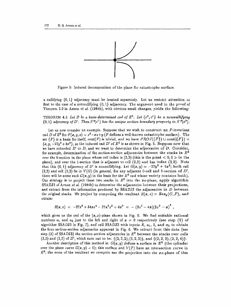
Figure 5: Induced decomposition of the plane for catastrophe surface.

a nullifying (0, 1} adjacency must be treated separately. Let us restrict a t ten t ion at first to the case of a nonnullifying {0, 1~ adjacency. The argument used in the proof of Theorem 2.2 in Arnon et aI. (1984b), with obvious small changes, yields the following:

THEOREM 4.1 Let D be a basis-de~ermined cad of E 3. Let (c s, c 1} be a nonnullifyin 9 (0, 1} adjacency o l d t. Then S~'(c 1) has the unique section boundary property in S ~(c°).

Let us now consider an example. Suppose that we wish to construct an F-invariant cad D o r e s for F($, y, z) -=- z3-~zq-y (F defines a well-known catastrophe surface). The set {F} is a basis for itself, cont(F) is trivial, and we have P R O J ( { F } ) U cor~t({F}) = {~,y, -27y2 +4z3}, so the induced cad D ~ o r e 2 is as shown in Fig. 5. Suppose now that we have extended D' to D, and we want to determine the adjacencies of D. Consider, for example, determination of the section-section adjacencies between the stacks in Ea over the 0-section in the plane whose cell index is (2,2) (this is the point < 0, 0 > in the plane), and over the 1-section that is adjacent to cell (2,2) and has index (3,2). Note that this {0, 1} adjacency of D' is nonnullifying. Let G(~, y) -= -27y 2 -b 4~s; bo th cell (3,2) and cell (2,2) lie in V(G) (in general, for any adjacent 0-cell and 1-section of D', there will be some such G(z, y) in the basis for the E 2 cad whose variety contains both) . Our strategy is to project these two stacks in E 3 into the ~z-plane, apply algori thm SSADJ2 of Arnon et al. (1984b) to determine the adjacencies between their projections, and extract from the information produced by SSADJ2 the adjacencies in D between the original stacks. We project by computing the resultant R(~, z) = Rest (G, F), and obtain:

= -27 +54 z' - 3 = - - -

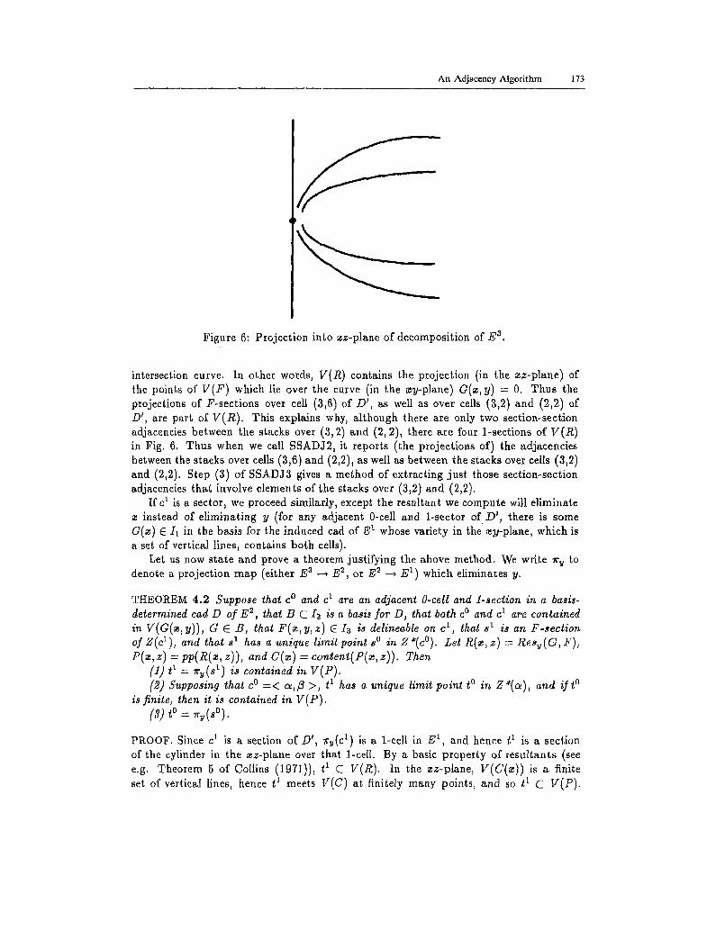
which gives us the cad of the (z,z)-plane shown in Fig. 6. We find suitable ra t ional numbers az and a2 just to the left and right of ~ = 0 respectively (see step (2) of algorithm SSADJ3 in Fig. 7), and call SSADJ2 with inputs R, al , 0, and a2 to ob ta in the four section-section adjaeencies apparent in Fig. 6. We extract from this da ta (see step (3) of SSADJ3) the section-section adjacencies in E ~ between the stacks over cells (3,2) and (2,2) of D', which turn out to be: {(2, 2, 2), (3, 2, 2)}, and {(2, 2, 2), (3, 2, 4)}.

Another description of this method is: G(z, y) defines a surface in E a (the cylinder over the plane curve G(z, y) = 0); this surface and V(F) have an intersection curve in E3; the zeros of the resultant we compute are the projection into the ~z-plane of this


Figure 6: Project ion into ~z-plane of decomposition of E a.

intersection curve. In other words, V(R) contains the projection (in the zz-plane) of the points of V(F ) which lie over the curve (in the ~y-plane) G(z ,y ) = 0. Thus the projections of F-sections over cell (3,6) of D' , as well as over cells (3,2) and (2,2) of D', are part of V(R) . This explains why, al though there are only two section-section adjacencies between the stacks over (3, 2) and (2, 2), there are four 1-sections of V(R) in Fig. 6. Thus when we call SSADJ2, it reports (the projections of) the adjaceneies between the stacks over cells (3,6) and (2,2), as well as between the stacks over cells (3,2) and (2,2). Step (3) of SSADJ3 gives a method of extracting just those section-section adjacencies that involve elements of the stacks over (3,2) and (2,2).

I r e 1 is a sector, we proceed similarly, except the resultant we compute will eliminate z instead of eliminating y (for any adjacent 0-cell and 1-sector of .D', there is some G(z) E 1~ in the basis for the induced cad of E t whose variety in the ~y-plane, which is a set of verticM lines, contains both cells).

Let us now state and prove a theorem justifying the above method. We write lr u to denote a projection map (either E s --~ E 2, or E 2 ~ E 1) which eliminates y.

THEOREM 4.2 Suppose that c ° and e 1 are an adjacent O-cell and 1-section in a basis- determined cad D o r e 2, thai B C [2 is a basis for" D~ that both e ° and c l are contained in V(G(~, y)), G E B, tha¢ F ( z , y, z) C I3 is delineable on c 1, that s t is an F-section of Z(cl), and that s t has a unique limit point s ° in Z*(c°). Let R(z, z) = Resu(G , F), P(~, z) = pp(R(~, z)), and C(~) = content(P(z, z)). Then

(1) i 1 = r~(s t) is contained in V(P). (2) Supposing that c o = < ~,13 >, t 1 has a unique limit point ~o in Z~(a), and if~ °

is finite, then it is contained in V(P) . Ca) t o = ~,(s°) .

PROOF. Since c 1 is a section of D', rru(c t) is a 1-cell in E 1, and hence t 1 is a section of the cylinder in the ~z-plane over that l-cell. By a basic proper ty of resul tants (see e.g. Theorem 5 of Collins (1971)), t 1 C V(R). In the zz-plane, V(C(~)) is a finite set of vertical lines, hence t 1 meets V(C) at finitely many points, and so t t C V(P).

174 D.S. Arnon et al,

Then since P (z , z) is primitive, our present context essentially satisfies the hypotheses of Theorem 2.2 of Arnon et al. (19845) (with P in place of the polynomial F($,y) that occurs there), hence by the argument used in the proof of Theorem 2.2, 11 has a unique limit point t ° in Z*(~) . If t o is finite, then it is in V(P) since Y(P) is closed. 7ru(s° ) is a limit point o f t l, and if it is not equal to t °, then t 1 has two distinct limit points in Z*(c~), which is impossible, n

Clearly there is a similar theorem for when c 1 is a sector. In that case, G(~, y) has positive degree in z (in fact is univariate in z), and we compute R(y,z) = Rest(G, F) instead of R(z, z) = Re%(G, F).

T h e hypotheses of Theorem 4.2 are clearly satisfied over any nonnullifying {0, 1} adjacency of D' , hence given any such adjacency {c°,ct}, we can apply SSADJ3 to determine the adjacencies between S*(c °) and S*(cl) . The precise specifications of $SADJ3 ' s inputs arc a consequence of the diverse contexts in which it is invoked.

Let us now note that the hypotheses of Theorem 4.2 do not exclude the possibility tha t c ° nullifies F. However, before we can be sure of the validity of the theorem for the case of a nullifying {0, 1} adjacency, ~e must verify tha t the hypothesis "s ~ has a unique limit point s o in Z*(ca)" holds in such a case. It is not hard to see that it must~ for clearly s 1 still has at least one limit point in Z*(e°), and if it had more than one, then so would wu(8 ~) have more than one limit point in lrv(Z*(e°)), which is clearly impossible. We m a y further observe that Theorem 4.2 tells us precisely wha~ (the z-coordinate of) s l ' s unique limit point in Z*(c °) is.

I t is enlightening to observe exactly how it happens that the conclusion of Theo- rem 4.2 still holds in the case tha t c o nullifies F. The key is the replacement of R(~, z) by its primitive par t P(~, z). It is not hard to convince oneself that for any primitive bivariate polynomial K(a, z), there is no value of ~ for which it is nullified. Thus, if c o nullifies F, then V(F) contains a "vertical line" over c o which we may think of "noise" obscuring the limit point of s 1 in Z*(c°), V(R) contains the projection of this "noise" (and so R is necessarily an imprimitive polynomial), but replacing R by its primit ive par t _P serves to filter out the "noise", and then since ~r~(8 z) C V(P) we can find s~'s limit point in Z*(c °) using SSADJ2.

Thus Theorem 4.2 yields the following corollary:

THEOREM 4.3 Suppose that D is a basis-determined cad of E a with basis B, and that £e °, c ~ } is a nullifying {0, 1} adjacency olD' such that e ° = < c~,~ >, and c 1 is a section contained in Y(G(a~, y)) for G($, y) ira the basis for D'. Suppose further, for every F e B which is nullified on c °, and every veal root 7 of pp( Res~( G, ;F) )( ~, z), that < ~, ~, 7 > is a section of the stack S(c °) in D. Then S*(c ~) has the unique section boundary property in S*(~°).

There is a similar theorem for the case of c 1 a sector. Thus if D is a cad of E 3 whose stacks were determined by algorithm E$tendCelIToStack, i.e. by a lgor i thm CelIE~tensionPolynomial, of Section 2, and if {c °, c 1} is a nullifying {0, 1} adjacency of D' , then S*(e t) has the USBP in S*(c°). Thus we can apply SSADJ3 in the nul- lifylng {0,1} case to determine the adjacencies between S*(c °) and S*(cl), jus t as in the nonnullifying case. Altogether we have the algorithm AdjacenciesOvev01 given in Fig. 8.


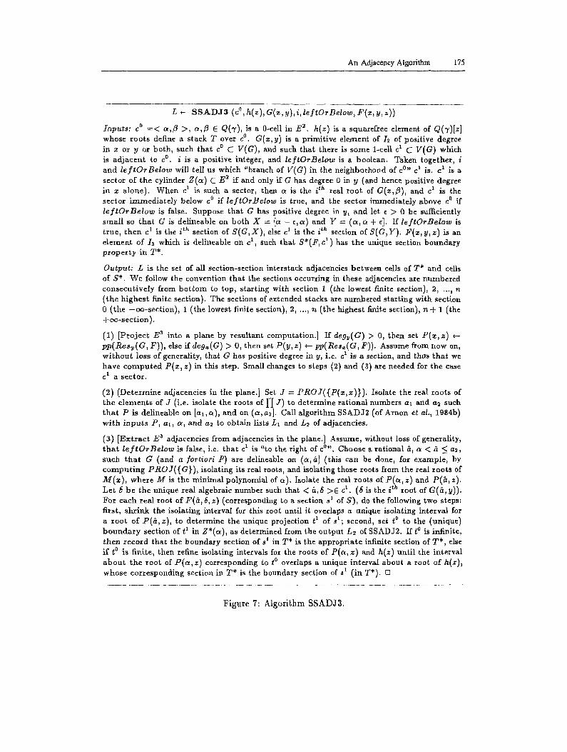
L ~-- S S A D J 3 (c D, h(z), G(z, y), i, leftOrBelow, P(z , y, z))

Inputs: c o = < c~,13 > , a,/3 E Q(7), is a 0-cell in E ~, h(z) is a squarefree element of Q(7)[z] whose roots define a stack T over c °. G(z ,y ) is a primitive element of 15 of positive degree in z or y or both, such that c o C V(G), and such that there is some 1-cell c t C V(G) which is ad jacent to c °. i is a positive integer, and leftOrBelow is a boolean. Taken together, i and lef tOrBelow will tell us which "branch of V(G) in the neighborhood of c o'' c 1 is. c 1 is a sector of the cylinder Z(c~) C E 2 if and only if G has degree 0 in y (and hence positive degree in z alone) . When c x is such a sector, then ~ is the i th real root of G(z,19), and c 1 is the sector immedia te ly below c o if leftOrBelow is true, and the sector immediately above c o if leftOrBelo~o is false. Suppose that G has positive degree in y, and let e > 0 be sufficiently smal l so tha t G is delineable on both X = [a - e ,a) and Y = ( a , a + el. If leftOrBelo~o is true, t hen c 1 is the i tn section of S(G, X), else c 1 is the i th section of S(G, Y). F(z , y, z) is an e lement of I3 which is delineable on c 1 , such that S*(F, c 1) has the unique section boundary p roper ty in T*.

Output: L is the set of all section-section interstack adjacencies between cells of T* and cells of S*. We follow the convention that the sections occurring in these adjacencies are numbered consecut ively from bo t tom to top, start ing with section 1 (the lowest finite section), 2, ..., n ( the highest finite section). The sections of extended stacks are numbered start ing with section O (the -co - sec t ion) , 1 (the lowest finite section), 2, ..., n (the highest finite section), n + ] (the +co-sec t ion) .

(1) [Project E a into a plane by resul tant computation.] ff deg~(G) > 0, then set P ( z , z ) e- pp(Res~ (a, F)), else ff deg=(G) > 0, then set P(y, z) ~-- pp(Res~(a, F)) . Assume from now on, wi thou t loss of generality, that G has positive degree in y, i.e. c 1 is a section, and thus tha t we have computed P(~ , z) in this step. Small changes to steps (2) and (3) are needed for the case C 1 a s e c t o r .

(2) [Determine adjacencies in the plane.] Set J = PROJ({P(z , z )} ) . Isolate the real roots of the e lements of J (i.e. isolate the roots of 1-] J ) to determine ra t ional numbers at and a~ such tha t P is delineable on [a~, c~), and on (a , a2]. Call a lgori thm SSADJ2 (of Arnort etal., 1984b) wi th i n p u t s P , at , tr, and a2 to obta in lists Lt and L2 of adjacencies.

(3) [Ext rac t E ~ adjacencies from adjacencies in the plane.] Assume, without loss of generality, t ha t lef tOrBelow is false, i.e. tha t c 1 is "to the right of e ° ' . Choose a rat ional ti, a < 5 < a2, such tha t G (and a fortiori P) are detineabie on (a,~] (this can be done, for example, by c o m p u t i n g PROJ({G}), isolating its real roots, and isolating those roots from the real roots of M ( z ) , where M is the min imal polynomial of a) . Isolate the real roots of P ( a , z) and P ( a , z). Let 6 be the unique real algebraic number such that < h,6 > e c ~. (6 is the i th root of G(5,y)). For each real root of F (5 , 6, z) (corresponding to a section s t of S), do the following two steps: first, sh r ink the isolating interval for this root unt i l it overlaps a unique isolating interval for a roo t of P ( a , z ) , to determine the unique projection t 1 of st; second, set t o to the (unique) b o u n d a r y section of t 1 in Z*(¢~), as determined from the output L2 of SSADJ2. If t o is infinite, then record that the boundary section of s t in T* is the appropriate infinite section of T*, else i f t o is finite, then refine isolating intervals for the roots of P(a, z) and h(z) unt i l the interval abou t the root of P(a,z ) corresponding to t o overlaps a unique interval about a root of h(z), whose corresponding section in T* is the boundary section of s 1 ( in T*). []

F igure 7: Algor i thm SSADJ3 .

176 D.S. Arnon et aL

L ~- Ad jaeenc i e sOver0 : t (c °, c 1 , B', B)

Inputs: c o = < a,/3 >, c~,/3 C Q(3'), is a 0-cell, and c t a 1-cell, in a cad D' of E 2 induced by a basis-determined cad D of E 3, such that {c°,c 1 } is an adjacency of D I. B' is a basis for D ~, and B is a basis for D.

Output: L is a list of all interstack adjacencies between S*(c °) and S(ct).

(1) [Section-sectlon interstack adjacencies: c ~ a section.] Set h(z) to the result of calling CeUEztenslonPolynomial(c°,B',B). If c ~ is a sector, then go to Step (2). Set /) e-- H B ' . Call SSADJ3 with inputs c °, h(z), B(z,y) , the appropriate value of i, the appropriate value of leftOrBelow, and I-[ B = B~ , to obtain output L*. Convert the section numbers that occur in the adjacencies of L* to indices of the corresponding cells of D, and add the resulting adjaceneies of D to L. Go to Step (3).

(2) [Section-section interstaek adjacencies: c ' a sector.] Let M(z) be the minimal polynomial of a. Set h(z) ~ CellEztensionPolynornial(c °,B', B). Call SSADJ3 with inputs c °, h(z), M(z), the appropriate value of i, the appropriate value of leftOrBelow, and [-[ B ~ B ~ to obtain output L*. Convert the section numbers that occur in the adjacencies of L* to indices of the corresponding cells of D, and add the resulting adjacencies of D to L.

(3) [Infer remaining interstack adjacencies.] Use the current contents of L to infer the remaining interstack adjacencies between S*(c °) and S(c~), and add them to L. D

Figure 8: Algor i thm kdjacenciesOver01.

5 Adjacenc ies over a nonnull i fylng {0,2} adjacency in the plane

As for T he o re m 4.1, the a rgument used to prove Theorem 2.2 of Arnon et al, (1984b) can be adap ted to prove the following:

THEOREM 5.1 Let D be a basis-determined cad of E ~. Let {c °, c 2} be a nonnullifying {0, 2} adjacency of D'. Then 5'*(c 2) has the unique section boundary property in S *(c°).

The following l e m m a will be useful in this and subsequent sections.

LEMMA 5.2 Let c o and c 2 be respectively a O-cell and a 2-cell in some cad of E ~, and suppose that c o is adjacent to c 2. Then there ezisL ezactly two 1-cells in the cad which are adjacent to both c o and c 2.

PROOF. Use a variat ion of the proof of L e m m a 5.10 in Massey (1978), p. 137-138. tD We call the two l-cells of Lamina 5.2 the "boundary 1-cells" of c 2 (with respect to

cO). Fig. 9 gives an algori thm to find them. Suppose now tha t O is a basis-determined cad of E a, and t h a t {e o, c 2} is a nonnul -

lifying {0, 2} adjacency of D'. Let c 1 be a b o u n d a r y 1-cell of c 2 with respect to e °. We have shown in Section 3 that S*(c 2) has the USBP in S*(el) , and in Section 4 tha t S*(e 1) has the USBP in S*(c°). Thus if s 2 is a section of S(c2), then s ~ has a unique b o u n d a r y section s 1 in S*(el) , attd s 1 has a unique boundary section s o in S*(c°) . I t follows tha t s o is adjacent to s ~, hence it must be the unique boundary section of 8 ~ in S*(c°). Thus to determine the section-section adjacencies between S(c °) and S(c2), it


(c~, c~) *-- B o u n d a r y O n e C e n s (c °, c 2)

Inputs: c o is a 0-cell, and c 2 a 2-cell, in a cad of E 2.

Output: c~ and c~ are the boundary 1-cells of c 2 with respect to c °.

(1) [Find "upper" boundary 1-cell] If the unique 1-section in the same stack as, and directly above, c 2 (this l-section may be either finite or infinite) has c o as its boundary 0-section in the (extension of the) stack containing c °, then set c~ to be this 1-section. Otherwise, set c~ to be the unique 1-sector that is in the same stack as1 and directly above, c °, and that is adjacent to both c o a n d c 2.

(2) [Find "lower" boundary 1-cell] If the unique 1-section in the same stack as, and directly below, c 2 (this l-section may be either finite or infinite) has c o as its boundary 0-section in the (extension of the) stack containing c °, then set c~ to be this l-section. Otherwise, set cl to be the unique 1-sector that is in the same stack as, and directly below, c °, and that is adjacent to both c o a n d c 2. O

Figure 9: Algorithm BoundaryOneCells .

suffices to pick a bounda ry 1-cell c t of c 2 with respect to c°~ and then find (in already cons t ruc ted adjacency information) all sections of S(c 1) which are adjacent bo th to a sect ion of S(c °) and to a section of S(c~). Fig. 10 gives the complete algorithm.

6 Adjacencies over a nullifying {0,2} adjacency in the plane

We would like for a stack in E ~ (over a cell c C E 2) to have the USBP in each adjacent lower-dimensional stack (more specifically, irt each stack over a cell d which meets 0c). As we have seen, we can achieve this goal over {1, 2}, nonnullifying {0~ 1}, nullifying {0, 1}, and nonnullifying {0, 2} adjacencies in E 2. It turns out tha t we cannot achieve this goal over nullifying {0, 2} adjacencies. For example, consider again F(~ , y, ~) = zz - y. In a typical F-invariant cad of E a, there will be a 2-section (whose base is the 2-cell "z > 0 A N D y > 0" in the induced cad of the plane) which has infinitely many bounda ry poin ts in the z-axis. The unique section boundary property cannot possibly be made to hold in such a case. However, there is a weaker, but still useful, proper ty t h a t we can make hold. Given adjacent stacks S and T in E' , we say that S* has the section boundary property (SBP) in T*, if for any section s of S*, the set of boundary points of s in the underlying cylinder of T* is equal to the union of one or more lower-dimensional e lements of T*. For a nullifying {0, 2} adjacency in E2~ if the stacks S and T over the 2-cell and 0-cell respectively are constructed according to the specifications we will give, then we can show that S* has the SBP in T* (Theorem 6.4). By extending the a r g u m e n t used to prove Theorem 2.3 of Arnon et al. (1984b), the following can then be shown. Suppose a stack S* has the SBP in a stack T*, let u be a sector of S*, and suppose that st and s2 are the respective sections of S* immediately below and above u. Let ~l be the "lowest" element of T* which is in the boundary of s 1, and let $2 be the "highest" element of T* which is in the boundary of s2. Then the set of boundary po in t s of u in the underlying cylinder of T* is equal to the union of all elements o f T*


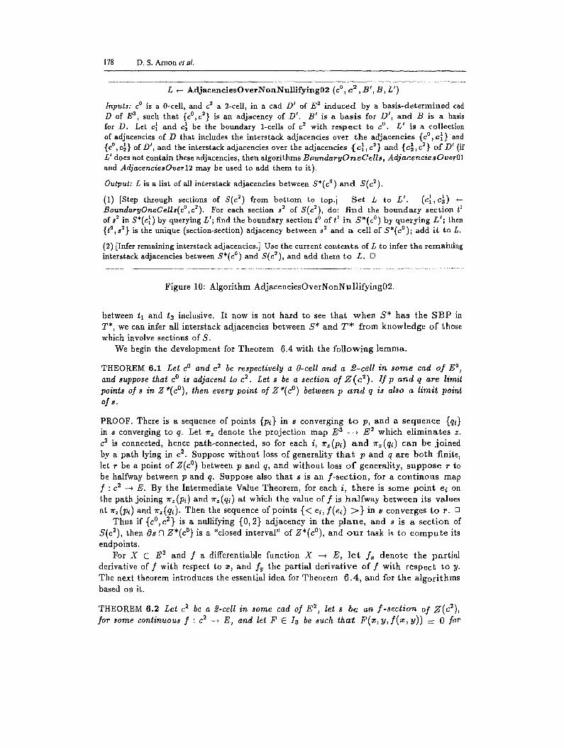
L ~ A d j a c e n c i e s O v e r N o n N u l l l f y l n g 0 2 (c °, c ~ , B ' , B, L')

Inputs: c o is a 0-cell, and c 2 a 2-cell, in a cad D' of E 2 induced by a basis-determined cad D of E a, such that {c°,c 2} is an adjacency of D I. B I is a bas is for D I, and B is a basis for D. Let c~ and c] be the boundary 1-cells of c 2 with respect to c o . L ~ is a collection of adjacencies of D that includes the interstack adjacencies over the adjacencies {c °, c~} and {c °, c~} of D', and the interstack adjacencles over the adjacencies {c~, c 2 } and {c~, c ~ } of D ' (if _U does not contain these adjacencies, then algorithms BoundaryOrLeCells~ AdjaeenclesOverO1 and Ad~acencieaOverl2 may be used to add them to it).

Output: L is a list of all interstack adjacencies between S*(c °) a n d S(c~).

(1) [Step through sections of S(c ~) from bottom to top.] Set L to L'. (c~,c~ t) ~- BoundaryOneCel ls(c° ,J) . For each section s 2 of S(c~), do: f ind the boundary section t 1 of s ~ in S*(c~) by querying L'; find the boundary section t o of t ~ in S*(c °) by querying L ' ; then {t°,s ~} is the unique (section-section) adjacency between s 2 and a cell of S*(c°); add it to L.

(2) [Infer remaining interstack adjacencies.] Use the current contents of L to infer ~he remaining interstack adjacencies between S*(c °) and S(c2), and add them flo L. []

Figure 10: Algori thm AdjacenciesOverNonNul l i fy ing02.

between tl and t~ inclusive. It now is not hard to see tha t w h e n S* has the S B P in T*, we can infer all interstack adjacencies between S* and T ~" f rom knowledge o f those which involve sections of S.

We begin the development for Theorem 6.4 with the fo l lowing lemma.

THEOREM 6.1 Let c o and c 2 be respectively a O-cell and a 2-ce l l in s o m e cad o f E 2, and suppose that c o is adjacent to c 2. f, et s be a section of Z ( e ~ ) . I f p a n d q are limit points of s in Z*(c°) , then every point of Z*(c °) between p a n d q is also a limi£ point o f s .

PROOF. There is a sequence of points {pl} in s converging t o p, and a sequence {ql} in s converging to q. Let Ir~ denote the projection map E s ~ E 2 which e l imina tes z. c 2 is connected, hence path-connected, so for each i, ~r~(pl) a n d 7rz(qi) can be joined by a path lying in c 2. Suppose without loss of generali ty t h a t p and q are bo th finite~ le~ r be a point of Z(c °) between p and q, and without loss o f generality, s u p p o s e r to be halfway between p and q. Suppose also tha t s is an f - s e c t i o n , for a c o n t i n o u s map f : c 2 ~ E. By the Intermediate Value Theorem, for each i, t he r e is some poin t el on the path joining 7r~ (p~) and ~-~(q~) at which the value of f is h a l f w a y be tween its values ~t 7r~(pl) and r~(qi). Then the sequence of points {< el, f ( e l ) :>} in s converges t o r. D

Thus if {c °, c 2} is a nullifying {0, 2} adjacency in the p l ane , and s is a sec t ion of S(c~), then Os n Z*(c °) is a "closed interval" of Z*(e°), and o u r task is to c o m p u t e its endpoiuts.

For X C E 2 and f a differentiable function X ~ E, l e t f~ deno te the par t ia l derivative of f with respect to z, and fy the partial der iva t ive of f with respec t to y. The next theorem introduces the essential idea for Theorem 6 .4 , and for the a lgor i thms based on it.

THEOREM 6.2 Let c 2 be a 2-cell in some cad of E 2, let s be an f - s e c t i o n of Z(c2) , for some continuous f : c 2 --* E, and let F e Ia be such t ha t F ( ~ , y , f(.~, y)) = 0 for


all< z ,y >E c 2. I f neither Fz nor F u nor F~ vanishes at any point of s, then f is differentiable, and the values of the functions fz and fu each are of constant nonzero sign throughout c ~.

PROOF. Since F, does not vanish at any point of s, by the Implicit Function Theorem f is differentiable on c 2, and

A - F.

on c 2. Since neither Fz nor F~ vanishes at any point of s, s is F~-invariant, and Fz- invariant. Hence fz is sign-invariant and nonzero on c 2. The same argument applies for

fv.~ Assume for a moment the hypotheses of Theorem 6.2. If F~ vanishes at a point

< a,/3,7 > of s, then by a basic property of resultants (see e.g. Theorem 5 of Collins, 1971), Resz(F, F~) vanishes at < a,/3 >. Hence if we knew tha t Resz(F, Fv) does not vanish at any point of c 2, then we would know tha~ F v does not vanish at any point of s. The same holds for Resz(F, Fz) and F,. We write PDP(F) to denote the set {Res,(F, F~), Res,(F, F,)}; P D P stands for "partial derivative projection".

THEOREM 6.3 Assume the hypotheses of Theorems 6.1 and 6.2. Let c~ and c~ be the boundary l-cells of c 2 with respect to c °, Suppose that s has unique boundary sections t~ and t~ in Z *(~-~) and Z *(4) respectively, and let pO and pO denote the (respective) limit points of t~ and t~ in Z*(c°). If neither element of PDP(F) vanishes at any point of c 2, then 0s A Z*(c °) is all points of Z*(c °) between pO and pO inclusive.

PROOF. Suppose first that both c( and c~ are sections. Obviously p0 and p0 are boundary points of s, and hence by Theorem 6.1, so are all points of Z*(c °) between them. If point p of Z*(c °) is a boundary point of s, then there is a sequence of points {p~} = {~i, Y~, f ( ~ , Yt)} in s converging to p. {~rz(p~)} = {~ , y~} is a sequence in c ~. Suppose that c~ is a gl-section, c~ is a g2-section, and without loss of generality, that gl < g2. Our hypothesis on PDP(F) implies, as observed a moment ago, that neither Fu nor F, vanishes at any point of s. Hence by Theorem 6.2, .fv is either positive or negative on c~; assume without loss of generality positive. Suppose that t~ is an fl-section, and that t~ is an f2-section. The sequence < ~,,gl(~i) , f l (zl ,gl(zl)) > converges to p0, and the sequence < ~i,gz(z~), f2(zi,g2(zi)) > converges to pO. Clearly f l(~, , gl(m,)) < f (z i ,y i ) < f2(zl,g2(~i)) for each i, and so p is between p0 and p0.

Suppose that c~ is a sector, and c~ a section. Imagine inserting a new 1-dimensional section which is in c 2, adjacent to e °, and very close to c~. Then we can apply the above argument. As this new section approaches c~, the boundary point of s over this section in Z*(c °) must approach the boundary point of t~ in Z*(c°), by the continuity o f / 7 Hence the conclusion of the theorem remains valid. The same argument can be used if c~ is a sector, or if both c~ and c~ are sectors. []

Let us see how to make use of Theorem 6.3. Assume its hypotheses, and suppose further that {c °, c z} is a nullifying {0, 2} adjacency in the plane. We are interested in the behavior of s close to Z*(c°), so actually it is not necessary that the elements of PDP(F) be nonvanishing at every point of c 2. It suffices tha t there be some ball in the plane, centered at c °, such that the elements of PDP(F) are nonvanishing at all points of the portion of c 2 inside the ball. If such a ball exists, then pO and p0 are the endpoints of the interval of boundary points of s in Z*(c°), and if p0 and p0 have been made sections of S*(c °) (by CADA3), then we can find them with two applications of


"--.. ~ " ~ ~ V(Res~ (F, Fy ) )

Figure 11: Ball of the desired kind exists.

SSADJ3. Fig. 11 illustrates the situation we might have in the plane when a ball of the desired kind exists. A ball of the desired kind fails to exist when either V(Res~(F, F~)) or V(Res,(F, F,)) or both have 1-sections that are between e~ and c~, and adjacent to c °, as depicted in Fig. 12. We handle this case by thinking of c 2 as being partitioned, in the neighborhood of c °, into 2-dimensional "subseetors" separated by these sections of V(Res~(F, Fy)) and V(Res,(F, F~)). This partit ion of c 2 induces a partition of s into 2-dimensional "subsections", separated by the 1-dimensional "slices" of s which lie over the sections of V(Res~(F, F~)) and V(Resz(F, Fz)). If we make the limit point in Z*(c °) of each "slice" of s a section of S*(c°), then by two applications of SSADJ3 for each "subsection" of s, we can find the boundary interval of that "slice" of s in Z*(e°). This is exactly what our algorithms (specifically, algorithm CelIE~tensionPolynor~ial of Section 2 ~nd algorithm AdjacenciesOverNullifying02 given below) do. Clearly the boundary interval of s in Z*(c °) is the union of the boundary intervals of its "subsections". AdjaeenciesOverN~llifying02 uses algorithm IntevioT'Sections, given in Fig. 13, to determine whether Y(Res~(F, Fy)) or V(Res~(F, F~)) has 1-sections tha t lie between c~ and c~ and are adjacent to c 0.

Theorem 6.4 summarizes our development.

THEOREM 6.4 Suppose that D is a basis-determined cad of E s with basis B, that {c°,c 2} is a nullifying {0,2} adjacency of D' with c o = < cqfl >, that the boundary 1-cells of c 2 with respect to c o are sections c~ and c~ of D I, contained respectively in V(GI(~, y)) and V(G2(~, y)), for elements G1 and G2 of the basis for D', and that for every F E B which is nullified on c°~ and for all real roots 7 of

(1) pp(n~s~ (F, al))(~, ~), (~) pp(~s~(F, v2))(~, ~), (s) pp(ae~(F, Rest(F, ~)))(~, ~), and (# pp(ne~ (F, ~e~(F, F~)))(~, ~),


cO I

Figure 12: Bal l of the desired kind fails to exist.

(i, j) ,-- I terlo Seetions (e °, c y))

Input#: c o = < c~,fl > is a O-cell, and c 2 a 2-cell, in a cad o r e 2. F(z , y ) is a primitive element o f / 2 .

Output: (i, j) is a pair of two non-negative integers. Assume, without loss of generality, that e 2 is "to the right of" c °. If i > 0, then for sufficiently small e, real roots i,i + 1~ ...,i + j of F(cx + e,y) correspond to l-cells contained in V(F), lying within c 2, that are between the boundary l-cells of c 2 with respect to c c, and that are adjacent to c °. If c 2 is "to the left of, c ° , then L = (i, j) refers to real roots of F(a - e, y), and small changes axe needed to the steps below.

(1) [Exit if F not of positive degree in y, or c o not contained in V(F).] If E not of positive degree in y, or if F(a,/3) # 0, then RETURN[ (0, 0)].

(2) [Find F-sections with required properties.] Do (c~,c~) ~ BoundaryOneCells(c °,c ~) to get the boundary l-cells of c ~ with respect to c °. Assume that both c~ and c~ are sections; small adjustments are needed if one or both are sectors. Suppose that c~ is real root rnz of Gz (a + e, y), and c~ is real root m2 of G2 (cx + e, y), for primitive polynomials G1 (z, y), G~ (z, y) of positive degree in y. Compute P -~ PROJ({F, Gi, G2~), and choose e so ~hat there are no r ea l roots of 1-I P in the interval J -= (a, a + el. It follows (Arnon et al., 1984a) that F , G~, G~, and FGIG2, are all delineable on J. If real roots i , i + ], . . . , i+ j o f F ( a + e , y ) lie between r o o t m~ of G~(a + e, y), and root ms of G2(c~ + c,y), then RETURN[ (i, j) ], else RETURN[ (o, o)]. o

Figure 13: Algor i thm InteriorSections.

182 D.S. Arnon et aL

< a,j3,7 > is a section of S(c°). Then S~(c 2) has the section boundary property in S*(c°).

When one (or both) of the boundary 1-cells, say c~, o f c u is a sector, a variant of Theorem 6.4 is needed. Given that c o = < ct,~ >, let M(m) E I1 be the minimal polynomial of a. The variant is obtained by replacing pp(Resu(F, G1))(~, z) with pp( Res~( F, M) )(fl, z).

We give algorithm AdjacenciesOverNullifying02 in Fig. 14. Note tha t i f{c °, c 2 } is a nullifying {0, 2} adjacency of D', then c o nullifies at least one e l emen t of B, but there may be other elements of B which are delineable, rather than nullified, on c °. I f s is a section ofS(c ~) in such a case, and if the unique element F of B, in whose variety s is contained, is not nullified on c °, then OsNZ*(c °) consists of a unique sec t ion of S*(c°), which can be determined by the method of Section 5. In fact, AdjacenciesOve~Nullifying02 handles such sections s in just this way.

7 M a i n a l g o r i t h m

We summarize thc preceding Sections with our main a lgor i thm CADA3, given in Fig. 15.

THEOREM 7.1 A cad of E 3 constructed by algorithm CADA 3 has the boundary property.

PROOF. Let D be the cad. It is clear from the defintion of a l g o r i t h m EztendCellToStack of Section 2 that D is a basis-detezmincd cad. By our discussion in Section 1, the induced cad D' o f E 2 constructed by algorithm CADA2 ofArnon et al. (1984b) has the boundary property. If {c, d} is an adjacency of D' , with dim(d) < dim(c), then by Theo rems 3.1, 4.1, 4.3, 5.1, and 6.4, S*(c) has either the USBP or the S B P in S*(d). I t follows that S*(c) has the boundary property in S*(d). Hence D has the bounda ry property. ~']

8 Example

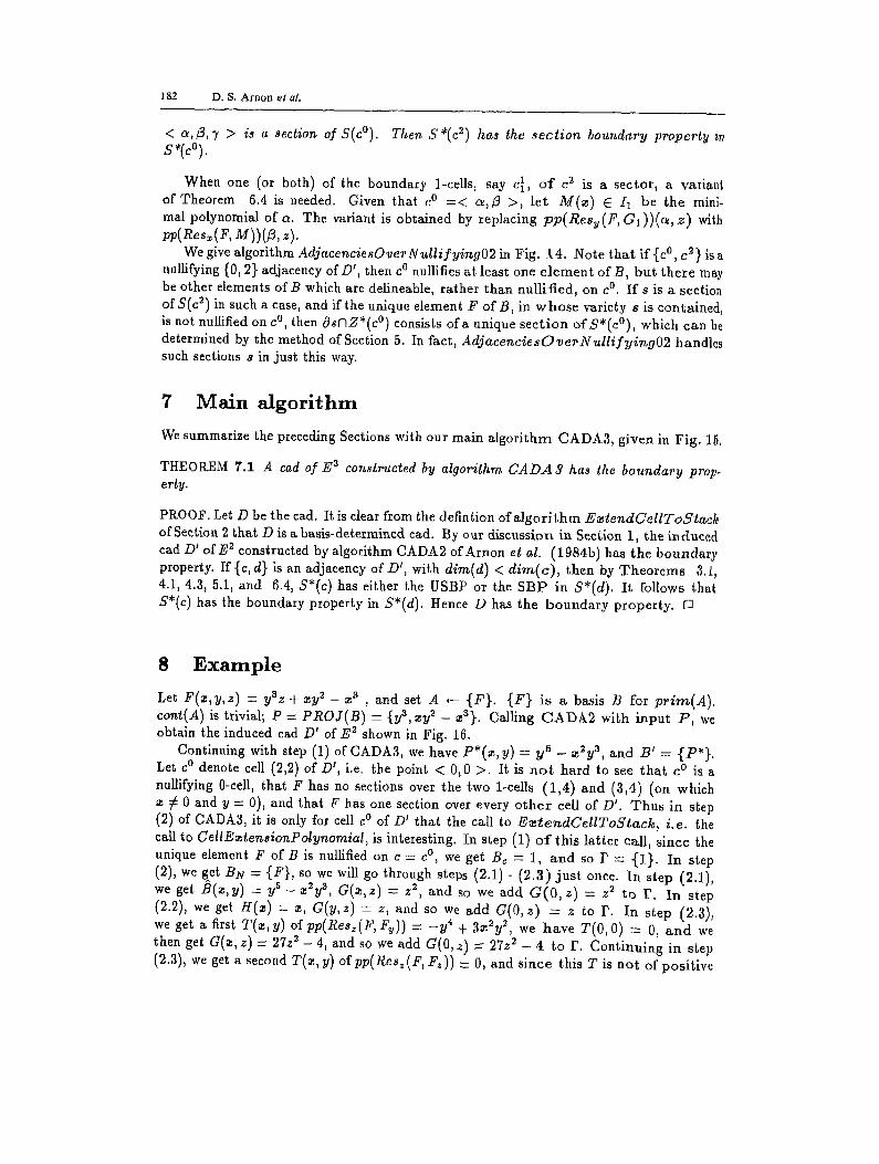
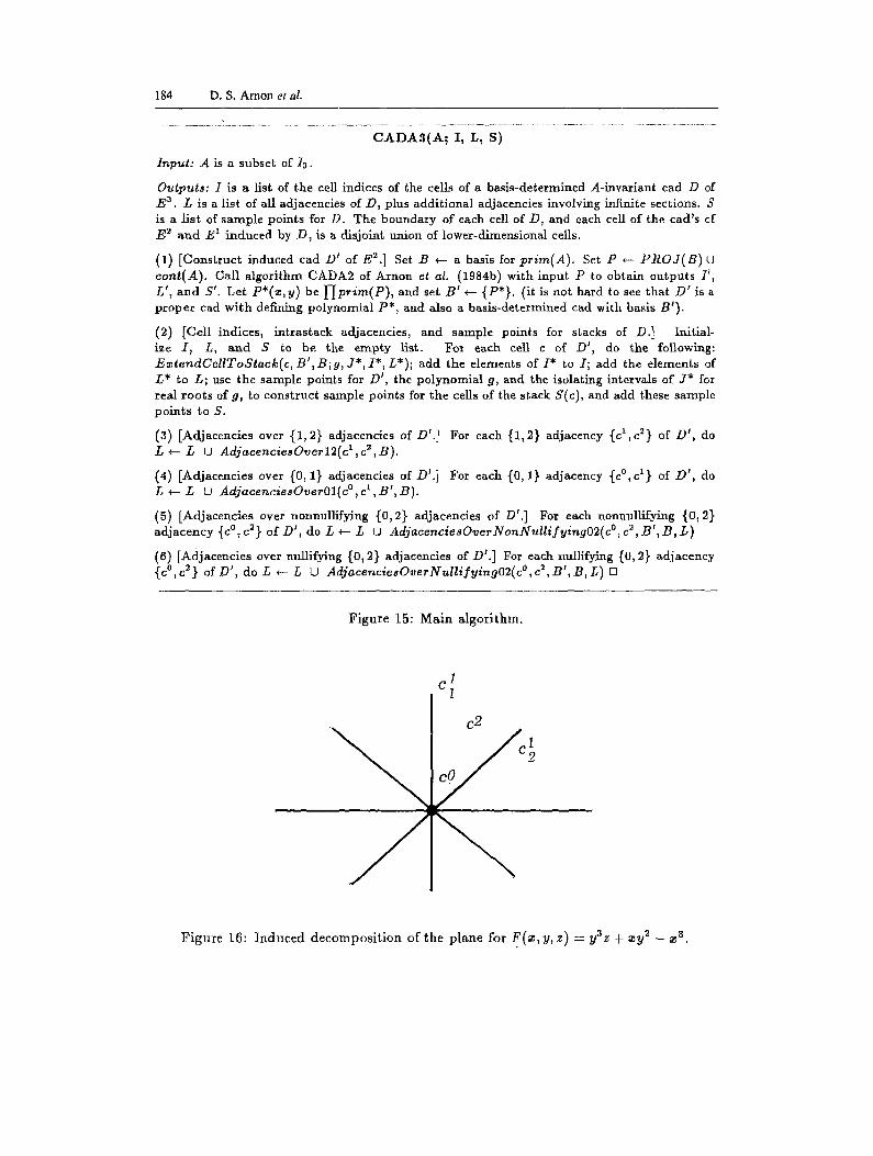
Let F(z,y,z) = yaz+my 2 - m s , and set A ~ {F}. {F} is a basis B for prim(A). cont(A) is trivial; P = PROJ(B) : {y3, my2 _ ms}. Calling C A D A 2 with input P , we obtain the induced cad D' of E 2 shown in Fig. 16.

Continuing with step (1) of CADA3, we have P*(m, y) -- yS _ ~ y a , and B ' -- {P*}. Let c o denote cell (2,2) of D 1, i.e. the point < 0,0 2>. It is n o t hard to see tha t e ° is a nullifying 0-cell, that F has no sections over the two 1-cells (1,4) and (3,4) (on which

¢ 0 and y = 0), and that F has one section over every o the r cell of D'. Thus in step (2) of CADA3, it is only for cell c o of D' that the call to Emter~dCellToStack, i.e. the call to CellEztensionPolynomial, is interesting. In step (1) o f this latter call, since the unique element F of B i s nullified o n c = c o , wege t Bc = 1, and so F = {1}. In step (2), we get BIv = {F}, so we will go through steps (2.1) - (2.3) jus t once. In step (2.1), we get B(~, y) = yS _ m~y~ a(m, z) = z', and so we add G(0 , ~) = ~ to r. In step (2.2), we get H(m) = m, a(y, ~) = ~, and so we add a(0, ~) = ,- to r. In stev (2.3), we get a first T(m,y) ofpp(Res~(F, Fu)) = _y4 + 3~2y2 we have T(0,0) = 0, a n d we then get G(~, z) = 27z 2 - 4, and so we add G(0, z) ~ 27z 2 - 4 to r . Continuing in step (2.3), we get a second T(m, y) of pp(Res~ (F, Fz)) = 0, and since this T is not of posit ive


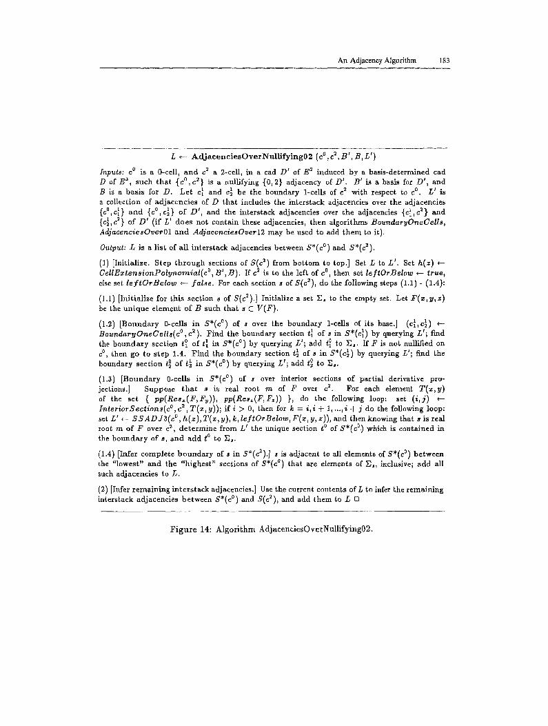
L e-- A d j a e e n e i e s O v e r N u l l i f y i n g 0 2 (c o , c a, B ' , B, L ' )

Inputs: c o is a 0-cell, a n d c 2 a 2-cell, in a cad D ~ of E a induced by a basis-determined cad D of E 3, such tha t { c ° , c 2} is a nullifying (0 ,2} adjacency of. D'. B' is a basis for D', and B is a bas is for D. Le t e~ and c~ be the boundary 1-cells o f c 2 with respect to c o . L ~ is a collection of ad jacenc ies of D tha t includes the in ters tack adjacencies over the adjacencies {c°,c~} and {c °, c~} of D ' , and the interstack adjacencies over the adjacencies {c~ ,J ] . and {c~, c a} of D' (if L' does not contain these adjacencies, then algori thms BoundaryOneCells, AdjacenciesOverO1 a n d AdjaceneiesOverl2 may be used to add t hem to it).

Output: L is a l is t of a l l in ters tack adjacencies between S*(e °) and S*(ca).

(1) [Initiali~.e. Step t h ro u g h sections of S(c ~) from b o t t o m to top.] Set L to L ' . Set h(z) ~-- CeUE~tensionPolynornial(e °, BlaB). If c a is to the left of c °, then set leftOrBelow e-- true, else set leflOrBelow ,-- false. For each section s of S(ea), do the following steps (1.1) - (1.4)"

(1.1) [htiLialize for this s e c t i o n , of S(ca).] Initialize a set ~ , to the empty set. Let F(z,y,z) be the un ique element of B such tha t s C V(F).

(1.2) [Boundary 0-cells in S*(c °) of s over the boundary a-cells of i ts base.] (c~,c~) e-- BoundaryOneCells(c °, c 2). F ind the boundary section t~ of s in S*(c~) by querying Lt; find the b o u n d a r y sect ion t ° of t l in S*(c °) by querying Z' ; add t o to ~Es. If 2 ~ is not nullified on C °, then go to s tep 1.4. F i n d the boundary section t~ of s in S*(c~) by querying L'; fred the boundary sect ion t o of t~ in S*(c °) by querying L' ; add t~ to ~ , .

(1.3) [Boundary 0-cells in S*(c °) of s over interior sections of par t ia l derivative projections.] Suppose t h a t s is real root m of F over c 2. For each element T ( z , y ) of the set { pp(Res~(F, Fy)), pp(Res~(F,f~)) }, do the following loop: set ( i , j ) e-- lnteriorSections(c °, c a , T ( z , y)); if i > 0, then for k -- i)i Jr 1 .... ,i-t-j do the following loop: set L ' ~-- SSADJ3(c °, h(z), T(z, y), k, leftOrBelow, F(z, y, z)), and then knowing that s is real root m of .F over c a, de t e rmine from L ~ the unique section t ° of S*(c°.) which is contained in the b o u n d a r y of t , and add t o to ~ .

(1.4) [Infer comple te b o u n d a r y of s in S*(ca).] s is adjacent to all elements of S*(c °) between the "lowest" and the "highest" sections of S*(c °) that are elements of D,, inclusive; add all such adjacencies to L.

(2) [Infer r ema in ing in t e r s t ack adjaceucies.] Use the current contents of L to infer the remain ing interstack adjacencies be tween S*(c °) and S ( J ) , and add them to L 13

F i g u r e 14: A l g o r i t h m Ad jacenc i e sOve rNu l l i f y ing02 .

184 D.S. Arnon et el.

CADA3(A; I, L, S)

Input: A is a subset of 13.

Outputs: I is a list of the cell indices of the cells of a basis-determined A-invariant cad D of E a. L is a l ist of all adjacencies of D, plus addit ional adjacencies involving infinite sections. S is a l is t of sample points for D. The boundary of each cell of D, and each cell of the cad's of E ~ and E i induced by D, is a disjoint union of lower-dimensional cells.

( I ) [Construct induced cad D ' of E2.] Set B ~-- a basis for prim(A). Set P ~-- P R O J ( B ) U coat(A). Call algori thm CADA2 of Arnon et al. (1984b) with input P to obtain outputs I ~, L ' , and S*. Let P*(~,y) be Hprim(P) , and set B ' e-- {P*}. (it is not hard to see that ]9' is a p roper cad with defining polynomial P*, and also a basis-determined cad with hasis B*).

(2) [Cell indices, intrastack adjacencies, and sample points for stacks of D.] Initial- ize I , L, and S to he the empty list. For each cell c of D', do the following: EztendCellToStack(c, B ' ,B;g, J*,I*, L*); add the elements of I* to I; add the elements of L* to L; use the sample points for D', the polynomial g, and the isolating intervals of J* for real roots of g, to construct sample points for the cells of the stack S(c), and add these sample points to S.

(3) [Adjacencies over {1, 2} adjacencies of D'.] For each {1,2} adjacency {c i ,c ~} of D', do L +-- JL U AdjacenciesOverl2(cl ,J ,B).

(4) [Adjacencies over {0, 1} adjacencies of D'.] For each {0, 1} adjacency {c °, c i} of 19', do L +-- L U AdjacenciesOverOl(c°,ci,B',B).

(5) [Adjacencies over nonnullifying {0,2} adjacencies of D'.] For each nonnullifying {O, 2} adjacency {c °, c 2 } of D ' , do L ~ L U AdjaceneiesOverNonNuUifying02(c °, c 2 , B', B,.L)

(6) [Adjacencies over nullifying {0, 2} adjacencies of D'.] Fo~ each nullifying {0, 2} adjacency {c °, c a } of D ' , do L ~- L U AdjacenciesOverNullifying02(c °, c 2, B', B, L) []

Figure 15: Ma in a lgor i thm.

Y

1 C 1

C2

2

Figu re 16: Induced decompos i t i on of the p lane for F ( ~ , y, z) = yaz + zy2 _ za.


Figure 17: Interior section in the plane for F(z,y ,z) = ySz + my2 _ ~ .

degree in y, we exit step (2.3). Given the r we have created, it is clear that in step (3) o f CeltE~tensionPolynomial we will obtain g(z) = z(27z 2 - 4). Thus returning to step (1) of E~iendCellToSiack where we isolate the real roots of g(z), the data returned b y E~tendCelIToS~ack will correspond to a stack in E s (over cell c °) that has three sections: the 0-cens < 0, 0, - 2 /3v r3 >, < 0, 0, 0 >, and < 0, 0, 2 / 3 v ~ >.

Let c 2 be the 2-cell (3,7) of Dt~ let s be tlle unique section of D over c 2, and let us consider the boundary of s in Z*(c°). Thus we are interested in the adjacencies f o u n d by that call to AdjacenciesOverNullifying02 in step (6) of CADAS, in which t h e first two inputs to AdjacenciesOverNulli]ying02 are c o and c 2. In step (1) of AdjacenciesOvevNulli.fying02 we will set h(z) to the same g(z) = 27z a - 4z that we h a d above, we will have leftOvBelow = false, and since s is the unique section of S(c2), we win go through steps (1.1) - (1.4) just once. Clearly the two boundary 1-cells o f c 2 are cell (2,3), which we will call c~, and (3,6), which we will call c~. In step (1.2) of AdjacenciesOvevNullifying02, we will find that the boundary section of s in S*(c~) is t h e unique finite section ~ of this stack, and that the boundary section t o oft~ in S*(c °) is the section < 0, 0, 0 > of S(c°). Also, the boundary section of s in S*(e~) is the unique f in i te section t~ of this stack, and the boundary section t ° of ~ in S*(c °) is the section < 0 ,0 ,0 > of S(e°). Hence at the end of step (1.2), we will have ~, = {< 0,0,0 >}.

In step (1.3) of Adjacenc~esOverNulIifying02, we will get the same T(~ ,y) ' s that we had in our trace of CelIEm~ensionPolynomial above; thus only the first Tim ,y) --- __y4 q_ 3z2y2 may lead to a nontrivial computation and result in InteriorSections, and indeed for this T(m, y), we get back a result of (3, 0) from Inte~'iorSec$ion~, telling us t h a t the third real root ofT(e, y) corresponds to a (1-dimensional) "section" of V(T) ~hat lies between the two boundary 1-cells ofc 2 and is adjacent to c °. It is not hard to see that th i s "section" of V(T) is the 1-cell ~, defined by the formula • > 0 AND y2 _ 3~2 = O, a n d indicated by the dotted line in Fig. 17.

Continuing in step (1.3) of AdjacenciesOverNulli~ying02, we make one c~tll to S.qAD:I3, and from it learn that section < 0, 0, -2 /3x /3 > of S(c °) is contained in t h e boundary of s. Hence at the end of step (1.3), we have I2,, _- {< 0,0,0 >, < 0, 0 , - 2 / 3 v ~ >}. In step (1.4), we infer that s is adjacent to all cells of S(e °) be-

186 D.S. Arnon et el.

tween < 0,0,0 > and < 0,0,-2/3Vr3 > inclusive, hence since < 0,0,0 > is cell (2,2,4) of this stack, and < 0 ,0 , -2 /3v /3 > is cell (2,2,2), this means that s (which is cell (3,7,2)) is adjacent to cells (2,2,2), (2,2,3), and (2,2,4) of S(c°). In step (2) of AdjacenciesOver.Nullifying02, we infer the remaining interstack adjacencies between S*(c °) and S(c2), i.e. that cell (3,7,1)is adjacent to cell (2,2,1), and that cell (3,7,3)is adjacent to cells (2,2,5), (2,2,6), and (2,2,7).

The reader may find that considering cross-sections of V(F) by planes of the form y = constant, for small positive constants, will help to understand the behavior of CADA3 for this example. Writing F in the form z = k(~) = (~3 _ y2~) / yS the local maxima and minima o f k occur when W(~) = 3~ 2 - y ' / y3 = O, i.e. y = :~ Vr~. Thus at a local maximum of k, z = (3~ ~ - ~ a ) / (3v/-~a) = 2 / 3v/3, and at a local minimum of k, z = - 2 / 3vf3, independent of the (positive) value of y. The local minima occur over points < z , y > in E 2 of the form < ~ , v / ~ >, which are points in c ~ when • > 0. Thus the point < 0 , 0 , - 2 / 3v/~ > in E ~ must be a boundary point of s. i t is examples such as this F(~, y, z) that make necessary the machinery of algorithm AdjaceuciesOverNullifying02 (and algorithm CellEztensionPolyuomial), rather than jus t the simpler algorithm AdjacenciesOverNonNullifying02

9 R e f e r e n c e s

Arnon, D. S., Collins, G. E., McCallum, S. (I984a). Cylindrical algebraic decomposition I: the basic Mgorlthm, S I A M J. Camp. 13/4, 865-877.

Amen, D. S., Collins, G. B., McCMlum, S. (1984b). CyHndrlcM algebraic decomposition II: an adjacency algorlthm for the plane, SIAM" J. Comp. 1:1/4, 878-889.

Amos, D. S. (1979). A cellular decomposition algorithm for semi-algebralc sets. Proceedings of an InternationM Symposlum on Symbolic and Algebraic Manipulation (EUROSAM '79). Springer Lee. Notes Camp. Sel. 7~., 301-315.

Arnon, D. S. (1981). Algori~hma ]or the Geometry of Semi-Algebraic Sets. PhD thesis, Teeh. Rapt. ~436~ Camp. Sol. Dept., Univ. Wisconsln-Madison.

Arnon, D. S. (1988). A cluster-based cylindrical algebraic decomposition algorithm..L Symb. Camp, 5, (this issue).

Collins, G. E. (1971). The calculation of multivariate polynomial resultants. J. Assoc. Camp. Mech .18 /4 , 515-532.

Collins, G. E. (1975). Quantifier eliminatlon for real closed fields by cylindrical algebraic decomposition. Proceedings of the Second GI Conference on Automata Theory and Formal Languages. Springer £ec. lgotes Camp. Sel. 3hi, 515-532.

Collins, G. E., Loos, R. G. K. (1982). Real zeros of polynomials. In (Buchberger, B., Loos, K., Collins, G. E., ads.) Computer Algebra - Symbolic and Algebraic Computation (Computing Supplemen~um 4), pp. 83-94. Vienna and New York: Sprlnger-Verlag.

Kaltofen, E. (1982). Polynomial factorizatlon. In (Buehberger, B., Loos, R., Collins, G. E., ads.) Compu£er Algebra - Symbolic and Algebraic Computation (Computing Supplementum 4), pp. 95-113. Vienna emd New York: Sprlnger-Verlag.

Kouen, D., Yap., C. K. (1985). Algebraic cell decomposition in NC. Proe. IEEE Conf. on Foundations of Camp. Set. (FOCS), 515-521.

]k~azsey W. S. (1978). Homology and Cohomolooy Theory. New York, NY: Marcel Dekker.


McCallum, S. (1979). Constructive Triangulation of Real Curves and Sur]aces. MSe thesis, Math. Dept., Univ. of Sydney, Australia.

McCallum, S. (1988). An improved projection operation for cylindrical algebraic decomposition of three-dlmensional space. J. Symb. Camp. 5, (this issue).

Prill, D. (1986). On approximation snd incidence in cylindrical Blgebralc decompositions. SIAM J. Camp. 15, 972-993.

Schwartz, J. T.~ Sharir~ M. (1983). On the 'piano movers' problem II. General techniques for computing topological properties of real algebraic manifolds. Adv. Applied Math. 4, 298-351.

Walker R. J. (1978). Algebraic Carves, New York, NY: Springer-Verlag.

An Adjacency Algorithm for Cylindrical Algebraic ... · An Adjacency Algorithm 165 Such cylindrical...

Documents

Transcript of An Adjacency Algorithm for Cylindrical Algebraic ... · An Adjacency Algorithm 165 Such cylindrical...