An Adaptive Strategy for the Restoration of Textured ... · 2 Department of Mathematics–CIRAM,...
21
Numer. Math. Theor. Meth. Appl. Vol. 6, No. 1, pp. 276-296 doi: 10.4208/nmtma.2013.mssvm15 February 2013 An Adaptive Strategy for the Restoration of Textured Images using Fractional Order Regularization R. H. Chan 1 , A. Lanza 2 , S. Morigi 3 and F. Sgallari 2, ∗ 1 Department of Mathematics, The Chinese University of Hong Kong, Shatin, Hong Kong. 2 Department of Mathematics–CIRAM, University of Bologna, Via Saragozza, 8, Bologna, Italy. 3 Department of Mathematics, University of Bologna, Piazza Porta San Donato, 5, Bologna, Italy. Received 1 March 2012; Accepted (in revised version) 15 May 2012 Available online 11 January 2013 Abstract. Total variation regularization has good performance in noise removal and edge preservation but lacks in texture restoration. Here we present a texture-preserving strategy to restore images contaminated by blur and noise. According to a texture de- tection strategy, we apply spatially adaptive fractional order diffusion. A fast algorithm based on the half-quadratic technique is used to minimize the resulting objective func- tion. Numerical results show the effectiveness of our strategy. AMS subject classifications: 65F10, 65F22, 65K10 Key words: Ill-posed problem, deblurring, fractional order derivatives, regularizing iterative method. 1. Introduction Noise reduction and deblurring are usually used in a pre-processing stage in image restoration to improve image quality. In this paper, we focus on texture preserving restora- tion of images corrupted by additive noise and spatially-invariant Gaussian blur. The most common image degradation model, where the observed data f ∈ n 2 is related to the underlying n × n image rearranged into a vector u ∈ n 2 , is f = Bu + e, (1.1) where e ∈ n 2 accounts for the random perturbations due to noise and B is a n 2 × n 2 matrix representing the linear blur operator. ∗ Corresponding author. Email addresses: (R. H. Chan), (A. Lanza), (S. Morigi), (F. Sgallari) http://www.global-sci.org/nmtma 276 c 2013 Global-Science Press
Transcript of An Adaptive Strategy for the Restoration of Textured ... · 2 Department of Mathematics–CIRAM,...

Numer. Math. Theor. Meth. Appl. Vol. 6, No. 1, pp. 276-296
doi: 10.4208/nmtma.2013.mssvm15 February 2013
An Adaptive Strategy for the Restoration of
Textured Images using Fractional Order
Regularization
R. H. Chan1, A. Lanza2, S. Morigi3 and F. Sgallari2,∗
1 Department of Mathematics, The Chinese University of Hong Kong, Shatin,
Hong Kong.2 Department of Mathematics–CIRAM, University of Bologna, Via Saragozza, 8,
Bologna, Italy.3 Department of Mathematics, University of Bologna, Piazza Porta San Donato,
5, Bologna, Italy.
Received 1 March 2012; Accepted (in revised version) 15 May 2012
Available online 11 January 2013
Abstract. Total variation regularization has good performance in noise removal and
edge preservation but lacks in texture restoration. Here we present a texture-preserving
strategy to restore images contaminated by blur and noise. According to a texture de-
tection strategy, we apply spatially adaptive fractional order diffusion. A fast algorithm
based on the half-quadratic technique is used to minimize the resulting objective func-
tion. Numerical results show the effectiveness of our strategy.
AMS subject classifications: 65F10, 65F22, 65K10
Key words: Ill-posed problem, deblurring, fractional order derivatives, regularizing iterative
method.
1. Introduction
Noise reduction and deblurring are usually used in a pre-processing stage in image
restoration to improve image quality. In this paper, we focus on texture preserving restora-
tion of images corrupted by additive noise and spatially-invariant Gaussian blur. The most
common image degradation model, where the observed data f ∈ Rn2
is related to the
underlying n× n image rearranged into a vector u ∈ Rn2
, is
f = Bu+ e, (1.1)
where e ∈ Rn2
accounts for the random perturbations due to noise and B is a n2 × n2
matrix representing the linear blur operator.
∗Corresponding author. Email addresses: r han�math. uhk.edu.hk (R. H. Chan),alanza�ar es.unibo.it (A. Lanza), serena.morigi�unibo.it (S. Morigi),fiorella.sgallari�unibo.it (F. Sgallari)
http://www.global-sci.org/nmtma 276 c©2013 Global-Science Press
An Adaptive Strategy for the Restoration of Textured Images 277
It is well known that restoring the image u is a very ill-conditioned problem and a
regularization method should be used. A popular approach determines an approximation
of u as the solution of the minimization problem
minu
n1p‖Bu− f ‖pp +
λ
q‖A(u)‖qq
o, (1.2)
where A is a regularization operator and λ is a positive regularization parameter that
controls the trade-off between the data fitting term and the regularization term [13,25,27].
For p = 2 and q = 2, we get the classical Tikhonov regularization [11,13]. This approach
enforces smoothness of the solution and suppresses noise by penalizing high-frequency
components, thus also image edges can be smoothed out in the process.
Numerous regularization approaches and advances numerical methods have been pro-
posed in the literature to better preserve edges, including alternating minimization algo-
rithms [1], multilevel approaches [16], non-local means filters [4].
A very popular choice in the literature for regularization is based on the total varia-
tion (TV) norm. Total variation minimization was originally introduced for noise reduc-
tion [7,25] and has also been used for image deblurring [14] and super-resolution image
reconstruction [17]. The TV regularization (ℓ2-TV) is obtained from (1.2) by setting p = 2,
q = 1 and A(u) the gradient magnitude of u. If we let ∇ui := (Gx ,iu, Gy,iu)T , with Gx ,i,
Gy,i representing the ith rows of the x and y-directional finite difference operators Gx , Gy ,
respectively, then the regularization term is defined by the TV-norm
‖u‖T V = ‖A(u)‖1 :=
n2∑
i=1
Æ(Gx ,iu)
2 + (Gy,iu)2.
The distinctive feature of TV regularization is that image edges can be preserved, but the
restoration can present staircase effects.
A variant of the ℓ2-TV regularization is the ℓ1-TV regularization which is obtained from
(1.2) by replacing the ℓ2 norm in the data-fitting term by ℓ1 norm:
minu{‖Bu− f ‖1+λ‖u‖TV}, (1.3)
see, e.g., [5,26–29] for discussions on this model. This model has a number of advantages,
including superior performance with non-Gaussian noise such as impulse noise, see [20].
However, it is well known that the ℓ1-TV regularization has problems in preserving tex-
tures, see [6,28].
In image denoising, recent works have dealt with this drawback mainly by two differ-
ent strategies. In [10] the ℓ2-TV model is adopted using a spatially variant regularizing
parameter λ, selected according to local variance measures. In [2], a fractional order
anisotropic diffusion model is introduced, which leads to a "natural interpolation" between
the Perona-Malik equations [22] and fourth-order anisotropic diffusion equations [15].
An adaptive fractional-order multi-scale model is proposed in [31,32], where the model is
applied to noise removal and the texture is detected by a variant of the strategy in [10].
278 R. H. Chan, A. Lanza, S. Morigi and F. Sgallari
The main goal of this work is to apply an adaptive fractional order regularization term
for the restoration of textured images corrupted by additive noise and blur. To achieve this
aim, we use a 2-phase approach. First we apply a suitable texture detection method on the
observed image to obtain a texture map. Then a fractional order regularization is applied
to the parts of the image which are characterized to be texture regions by the map and
the classical TV regularization (ℓ1-TV) is applied elsewhere. In particular, we propose to
replace the TV regularization term ‖u‖TV in (1.3) with a spatially adaptive fractional order
TV regularization term, thus integrating the following four ingredients:
• use of the fractional order α of derivatives to better preserve textures,
• spatial adaptivity of α in order to allow flexibility in choosing the correct regularizing
operator,
• spatial adaptivity of λ in order to locally control the extent of restoration over image
regions according to their content,
• an effective texture detection methodology based on the noise auto-correlation en-
ergy which makes no assumption about the noise level of the image.
The paper is organized as follows. We describe the proposed adaptive fractional model
for image restoration in Section 2. An iterative solution of the proposed model obtained by
the half-quadratic strategy and its numerical aspects are discussed in Section 3. In Section
4 we briefly illustrate the computational aspects related to the fractional order derivatives
and in Section 5 we describe the texture detection method we used. Numerical examples
and comments are provided in Section 6 and the paper is concluded in Section 7.
2. The proposed adaptive model
We propose to modify the functional in (1.2) to the following adaptive fractional vari-
ational model
minu{‖Bu− f ‖1 + ‖ΛAα(u)‖1}, (2.1)
where Λ = diag(λ1, · · · ,λn2) is an n2×n2 diagonal matrix with λi representing the regular-
ization parameter for the ith pixel, Aα(ui) = ‖∇αi ui‖2, where αi represents the fractional
order of differentiation for the ith pixel and
∇αi ui := (Gαi
x ,iu, G
αi
y,iu)T (2.2)
is the fractional-order discrete gradient operator, with components representing the x and
y-directional fractional finite difference operators.
Let us motivate our model by analyzing the high-pass filtering character of the frac-
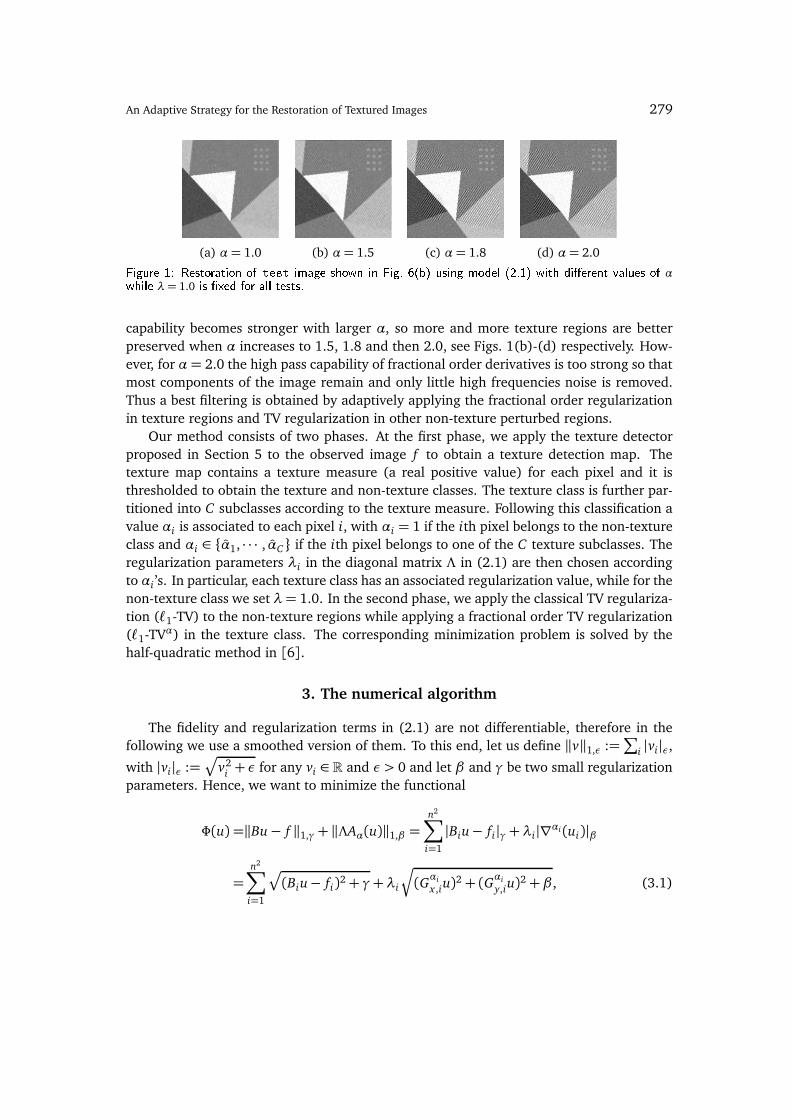
tional order derivative operator. In Fig. 1 we show the restored images of the blurred and
noisy test image in Fig. 6(b) by applying model (2.1) with different α while keeping
λ = 1.0. With α = 1 we get the ℓ1-TV model (1.3) which preserves edges but fails to
preserve fine scale features such as textures in the images, see Fig. 1(a). The high-pass
An Adaptive Strategy for the Restoration of Textured Images 279
(a) α = 1.0 (b) α = 1.5 (c) α = 1.8 (d) α = 2.0Figure 1: Restoration of test image shown in Fig. 6(b) using model (2.1) with di�erent values of αwhile λ = 1.0 is �xed for all tests.capability becomes stronger with larger α, so more and more texture regions are better
preserved when α increases to 1.5, 1.8 and then 2.0, see Figs. 1(b)-(d) respectively. How-
ever, for α = 2.0 the high pass capability of fractional order derivatives is too strong so that
most components of the image remain and only little high frequencies noise is removed.
Thus a best filtering is obtained by adaptively applying the fractional order regularization
in texture regions and TV regularization in other non-texture perturbed regions.
Our method consists of two phases. At the first phase, we apply the texture detector
proposed in Section 5 to the observed image f to obtain a texture detection map. The
texture map contains a texture measure (a real positive value) for each pixel and it is
thresholded to obtain the texture and non-texture classes. The texture class is further par-
titioned into C subclasses according to the texture measure. Following this classification a
value αi is associated to each pixel i, with αi = 1 if the ith pixel belongs to the non-texture
class and αi ∈ {α1, · · · , αC} if the ith pixel belongs to one of the C texture subclasses. The
regularization parameters λi in the diagonal matrix Λ in (2.1) are then chosen according
to αi ’s. In particular, each texture class has an associated regularization value, while for the
non-texture class we set λ= 1.0. In the second phase, we apply the classical TV regulariza-
tion (ℓ1-TV) to the non-texture regions while applying a fractional order TV regularization
(ℓ1-TVα) in the texture class. The corresponding minimization problem is solved by the
half-quadratic method in [6].
3. The numerical algorithm
The fidelity and regularization terms in (2.1) are not differentiable, therefore in the
following we use a smoothed version of them. To this end, let us define ‖v‖1,ε :=∑
i |vi|ε,
with |vi|ε :=p
v2i+ ε for any vi ∈ R and ε > 0 and let β and γ be two small regularization
parameters. Hence, we want to minimize the functional
Φ(u) =‖Bu− f ‖1,γ+ ‖ΛAα(u)‖1,β =
n2∑
i=1
|Biu− fi |γ+λi|∇αi(ui)|β
=
n2∑
i=1
p(Biu− fi)
2+ γ+λi
q(Gαi
x ,iu)2 + (G
αi
y,iu)2 + β , (3.1)

280 R. H. Chan, A. Lanza, S. Morigi and F. Sgallari
where Bi is the ith row of B, fi is the intensity of the ith pixel of the observed image.
The minimization of the functional (3.1) is obtained in a way similar to what is done for
the half quadratic ℓ1-TV [6,9,19]. Half-quadratic regularization is based on the following
expression for the modulus of a real, nonzero number x :
|x |=minv>0
nv x2+
1
4v
o, (3.2)
whose minimum is at v = 1/(2|x |) and the function inside the curly bracket in (3.2) is
quadratic in x but not in v; hence the name half-quadratic. By using (3.2), the minimum of
the function in (3.1) can be determined by minimizing the L operator defined as follows:
minuΦ(u) =min
u
n2∑
i=1
�|Biu− fi |γ+λi|∇
αiui |β�
=minu
n2∑
i=1
hminwi>0
�wi|Biu− fi |
2γ+
1
4wi
�+λi min
vi>0
�vi|∇
αiui |2β +
1
4vi
�i
= minu,v>0,w>0
n2∑
i=1
hwi |Biu− fi |
2γ+
1
4wi
+λi
�vi|∇
αiui |2β +
1
4vi
�i
:= minu,v>0,w>0
L (u, v, w). (3.3)
In order to solve (3.3), we apply the alternating minimization procedure, namely, for k =
0,1, · · · , we solve successively
v(k+1) = argminv>0L (u(k), v, w(k)), (3.4a)
w(k+1) = argminw>0L (u(k), v(k+1), w), (3.4b)
u(k+1) = argminu>0L (u, v(k+1), w(k+1)). (3.4c)
The first two minimizations in (3.4) have explicit solutions for each iteration:
v(k+1)
i=
1
2|∇αi u
(k)
i|−1β
, w(k+1)
i=
1
2|Biu
(k) − fi|−1γ . (3.5)
Since L (u, v(k+1), w(k+1)) is continuous differentiable in u, the solution u(k+1) of the third
minimization in (3.4) is obtained by imposing
0=∇uL (u, v(k+1), w(k+1))
=(Gα)T bΛbDβ(u(k))Gαu+ BT Dγ(u(k))(Bu− f ), (3.6)
where Gα := (Gαx ; Gαy ) ∈ R2n2×n2
is the discretization matrix of the adaptive fractional gra-
dient operator, bΛ := diag(Λ,Λ) ∈ R2n2×2n2
is a diagonal matrix of the adaptive regulariza-
tion parameters, bDβ (u(k)) := diag(Dβ(u(k)), Dβ(u
(k))) ∈ R2n2×2n2
, where Dβ(u(k)) ∈ Rn2×n2

An Adaptive Strategy for the Restoration of Textured Images 281
and Dγ(u(k)) ∈ Rn2×n2
are diagonal matrices with their ith diagonal entries being
(Dβ(u(k)))i = 2v
(k+1)
i= |∇αiu
(k)
i|−1β
, (3.7a)
(Dγ(u(k)))i = 2w
(k+1)
i= |Biu
(k) − fi |−1γ , (3.7b)
respectively.
Algorithm 3.1 outlines the computations for the adaptive fractional method for solving
(3.3).Algorithm 3.1: Adaptive-Fra tional (AF) AlgorithmInput: degraded image f , number of texture lasses C;Output: approximate solution u(k) of (3.3);1. {λi, αi , i = 1, · · · , n2 } = T D( f , C) ompute the texture-adaptive parameters on the de-graded image f ;2. Initialize the iterative pro ess by setting u(0) = f ;3. For k = 1,2, · · · until onvergent, solve�(Gα)T bΛ bDβ (u(k))Gα + BT Dγ(u
(k))B�
u(k+1) = BT Dγ(u(k)) f (3.8)endfor
The linear system of Eq. (3.8) is solved by the conjugate gradient method where we
terminate the iterations as soon as the norm of the residual is less than or equal to 10−4.
The use of an iterative solver allows us to avoid storing the large dimension matrices B
and Gα; the only requirement is matrix-vector products. In particular, the product which
involves matrix B makes use of FFT convolution, while the product by Gα is done according
to (4.5), described in Section 4. This makes it possible to solve large-scale problems on
fairly small computers. The texture detection procedure, step 1 in Algorithm 3.1, will be
outlined in Section 5.
The model (2.1) allows the use of the proof techniques in [6] to prove the convergence
of sequence {u(k)} to the minimum of Φ(u), as illustrated by the following result.
Theorem 3.1 (Convergence). For the sequence u(k) generated by the half-quadratic AF algo-
rithm, if
ker((Gα)T Gα)∩ ker(BT B) = {0}, (3.9)
then we have
(i) {Φ(u(k))} is monotonic decreasing and convergent;
(ii) limk→∞ ‖u(k) − u(k+1)‖2 = 0;
(iii) {Φ(u(k))} converges to the unique minimizer u∗ of Φ(u) from any initial guess u(0).
282 R. H. Chan, A. Lanza, S. Morigi and F. Sgallari
We remark that, in our case, for α ∈ [1,2], ker((Gα)T Gα) is spanned at most by the
two vectors: 1n2 , an n2 vector of ones and (1,2, · · · , n2), while the blurring matrix B is a
low-pass filter. Thus (3.9) always holds.
4. Fractional-order derivatives of variable α order
In this section, in order to allow for a complete overview of the discrete numerical
procedure for computing the matrix-vector product�(Gα)T bΛbDβGα�u(k+1) in (3.8), we will
explain how the fractional order derivatives have been discretized and made spatially-
adaptive by using variable fractional order.
Fractional-order derivatives have a long history and can be seen as a generalization of
the integer-order derivatives. Many definitions of fractional-order derivative exist and all
are consistent in some respect with the integer-order one. One of the most popular is the
frequency domain definition [8,21].
Since images are functions defined on a bounded domain, the computation of the
fractional-order partial derivatives by the discrete Fourier transforms requires that the
function must be symmetric and even, so that a prolongation of the image has to be
implemented. This yields a high computational cost. Moreover, here we are interested
in variable-order fractional differentiation, i.e., in the computation of spatially-adaptive
fractional-order derivatives. In this case the fractional order derivatives in the frequency
domain should be properly reconsidered.
Hence, following [30], in this paper we use the Grunwald-Letnikov fractional-order
derivative [23]. Let an image be an n× n matrix with i and j denoting the column and the
row pixel coordinates. The discrete, fractional-order gradient at a pixel (i, j) is defined as
(∇αi, j u)i, j =�(∆αi, j
x u)i, j, (∆αi, j
y u)i, j�, where
(∆αi, j
x u)i, j=
K−1∑
s=0
ωαi, j
s ui−s, j , (∆αi, j
y u)i, j=
K−1∑
s=0
ωαi, j
s ui, j−s , αi, j ∈ R+, (4.1)
with K > 0 being the number of pixels used for the approximation and ωαs , for a generic
α= αi, j , being the real coefficients defined as
ωαs =(−1)s�α
s
�=(−1)s
Γ(α+ 1)
Γ(s+ 1)Γ(α− s+ 1), α ∈ R+, s ∈ N. (4.2)
The generalized binomial coefficients�α
s
�, defined in (4.2) in terms of the Gamma function,
can be computed by the following recurrence relationships
�α
0
�= 1;
�α
s
�=
�α
s−1
�·�
1−α+ 1
s
�, α ∈ R+, s = 1,2, · · · . (4.3)
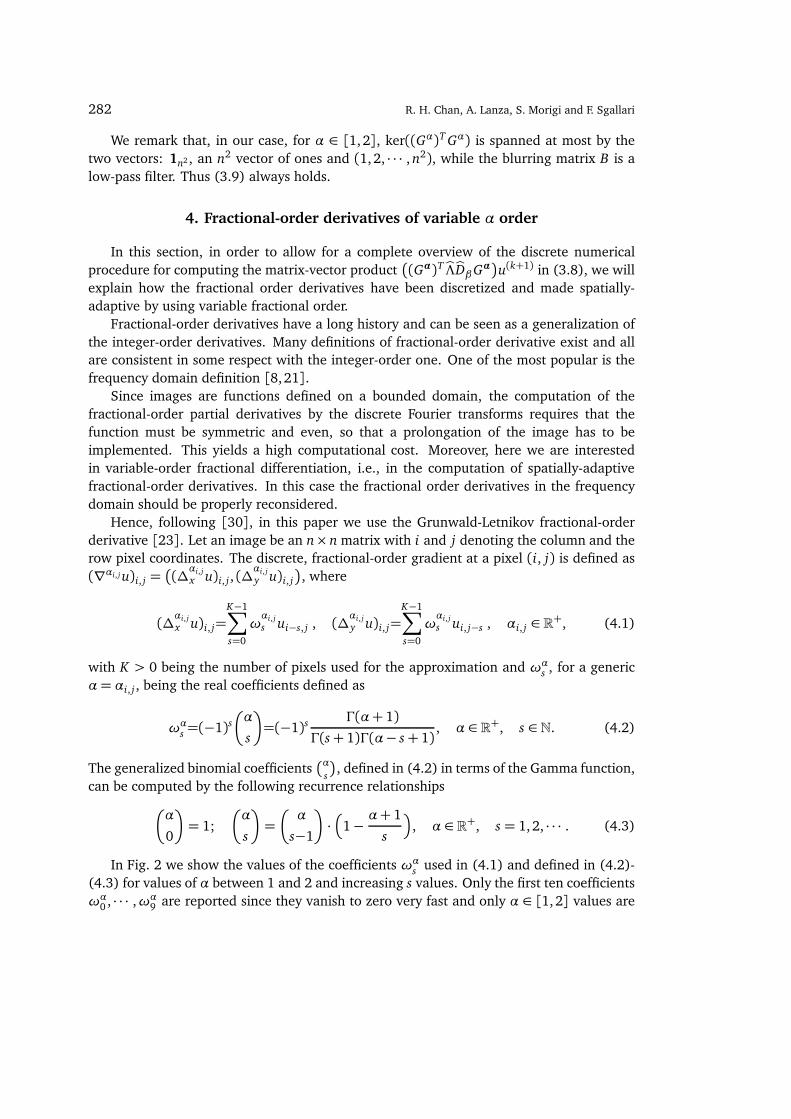
In Fig. 2 we show the values of the coefficients ωαs used in (4.1) and defined in (4.2)-
(4.3) for values of α between 1 and 2 and increasing s values. Only the first ten coefficients
ωα0 , · · · ,ωα9 are reported since they vanish to zero very fast and only α ∈ [1,2] values are
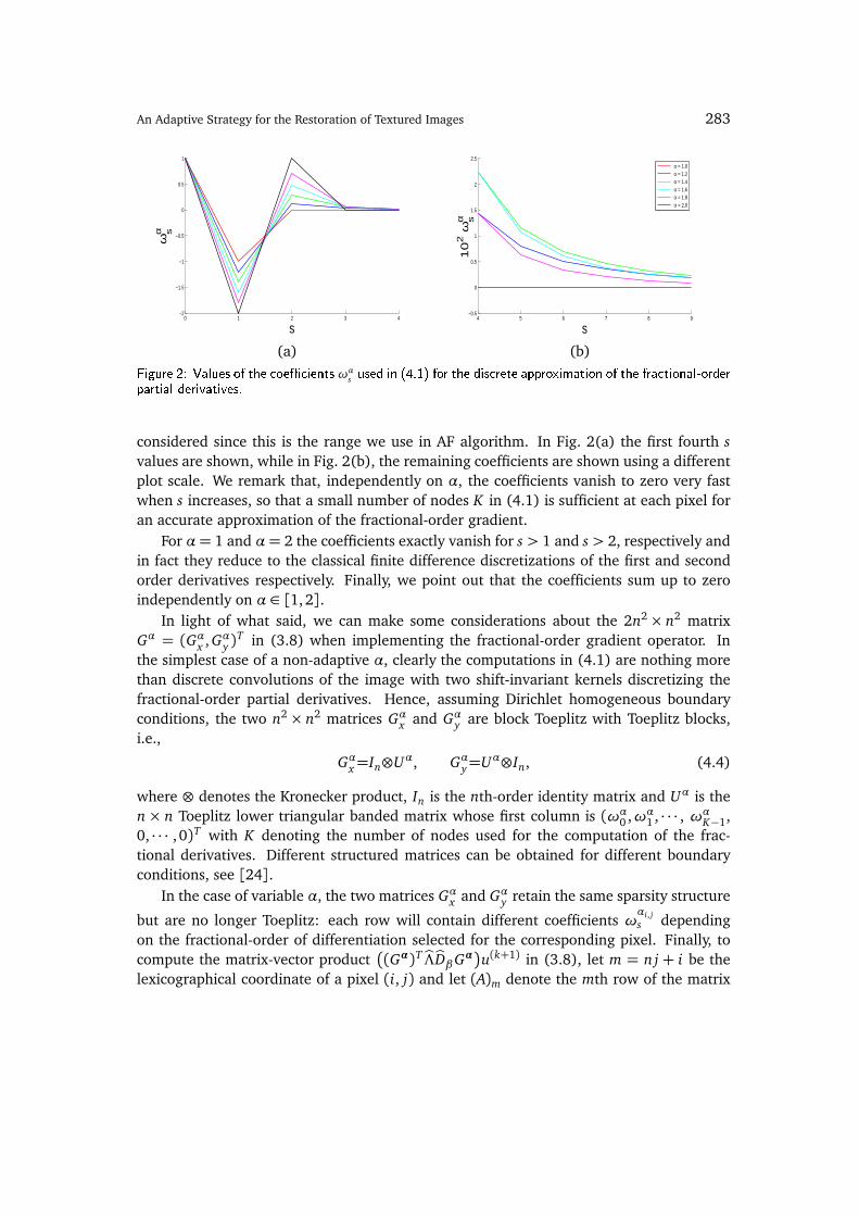
An Adaptive Strategy for the Restoration of Textured Images 283
0 1 2 3 4−2
−1.5
−1
−0.5
0
0.5
1
s
ωα s
4 5 6 7 8 9−0.5
0
0.5
1
1.5
2
2.5
s
10
2 ω
α s
α = 1.0 α = 1.2 α = 1.4 α = 1.6 α = 1.8 α = 2.0
(a) (b)Figure 2: Values of the oe� ients ωαsused in (4.1) for the dis rete approximation of the fra tional-orderpartial derivatives.
considered since this is the range we use in AF algorithm. In Fig. 2(a) the first fourth s
values are shown, while in Fig. 2(b), the remaining coefficients are shown using a different
plot scale. We remark that, independently on α, the coefficients vanish to zero very fast
when s increases, so that a small number of nodes K in (4.1) is sufficient at each pixel for
an accurate approximation of the fractional-order gradient.
For α= 1 and α= 2 the coefficients exactly vanish for s > 1 and s > 2, respectively and
in fact they reduce to the classical finite difference discretizations of the first and second
order derivatives respectively. Finally, we point out that the coefficients sum up to zero
independently on α ∈ [1,2].
In light of what said, we can make some considerations about the 2n2× n2 matrix
Gα = (Gαx , Gαy )T in (3.8) when implementing the fractional-order gradient operator. In
the simplest case of a non-adaptive α, clearly the computations in (4.1) are nothing more
than discrete convolutions of the image with two shift-invariant kernels discretizing the
fractional-order partial derivatives. Hence, assuming Dirichlet homogeneous boundary
conditions, the two n2 × n2 matrices Gαx and Gαy are block Toeplitz with Toeplitz blocks,
i.e.,
Gαx=In⊗Uα, Gαy=Uα⊗In, (4.4)
where ⊗ denotes the Kronecker product, In is the nth-order identity matrix and Uα is the
n× n Toeplitz lower triangular banded matrix whose first column is (ωα0 ,ωα1 , · · · , ωαK−1,
0, · · · , 0)T with K denoting the number of nodes used for the computation of the frac-
tional derivatives. Different structured matrices can be obtained for different boundary
conditions, see [24].
In the case of variable α, the two matrices Gαx and Gαy retain the same sparsity structure
but are no longer Toeplitz: each row will contain different coefficients ωαi, j
s depending
on the fractional-order of differentiation selected for the corresponding pixel. Finally, to
compute the matrix-vector product�(Gα)T bΛbDβGα�u(k+1) in (3.8), let m = n j + i be the
lexicographical coordinate of a pixel (i, j) and let (A)m denote the mth row of the matrix
284 R. H. Chan, A. Lanza, S. Morigi and F. Sgallari
A, then the m-th element of the resulting vector is
�(Gα)T bΛbDβGα�
mu(k+1)
=λi, j
�K−1∑
s=0
ωαi, j
s
(∆αi, j
x u(k+1))i+s, j
|∇αi, j u(k)
i+s, j|β
+
K−1∑
s=0
ωαi, j
s
(∆αi, j
y u(k+1))i, j+s
|∇αi, j u(k)
i, j+s|β
�, (4.5)
with the fractional finite difference operators ∆αi, j
x and ∆αi, j
y defined in (4.1).
5. Texture detection method
An automatic texture detection procedure was proposed in [10] where the noise is
assumed to be Gaussian with known variance and the authors use the ℓ2-TV denoising
method to detect texture regions in noisy images. Here, we present a new strategy for
computing a measure of texture at each pixel of a degraded image based only on the
assumption that the additive noise e in (1.1) is the realization of a white random process.
We make no assumption about the noise distribution and the noise variance. We only
assume that the noise is not correlated to the image and to itself.
Our idea is to use the auto-correlation function to detect non-whiteness in data.
Inspired by [10], starting from the observed degraded image, i.e., u(0) = f , we apply a
simple TV-flow with Neumann homogeneous boundary conditions
u(k+1)=u(k)+τ∇·�∇u(k)
|∇u(k)|
�, (5.1)
which approaches a piecewise constant image, so-called "cartoon model", that we denote
by u(k). The oscillatory parts removed by the TV flow are the noise e and the "non-cartoon"
part, that is the texture parts unc, which represent small-scale geometric details in the im-
age, see [28] for a detailed analysis of the ℓ1-TV model for decomposing a real image into
the sum of cartoon and texture. Under this decomposition, the residual can be represented
as
r(k) := f − u(k) = unc + e.
The sequence u(k) converges asymptotically to the constant image with value the mean
of the input image f (that we denote by f ), so that the corresponding r(k) approaches to
f − f , We want to stop the TV flow at a characteristic scale ek which allows us to well detect
textured parts unc in the image. Unlike the heuristic criterium adopted in [10], we propose
to consider the auto-correlation of the residue r(k) and to choose ek accordingly.
To describe the details of the approach, we briefly introduce some required statistical
concepts. Let E = {Ei, j : i, j = 1, · · · , n} be an n×n discrete random field with Ei, j denoting
the scalar random variable modeling noise at pixel (i, j). The auto-correlation of E is a
function ρE mapping pairs of pixel locations (i1, j1), (i2, j2) into a scalar value that must
lie in the range [−1,1], which represents the Pearson’s correlation coefficient between the
An Adaptive Strategy for the Restoration of Textured Images 285
two corresponding random variables Ei1, j1, Ei2, j2
, i.e.,
ρE[i1, j1, i2, j2]=E��
Ei1, j1−µi1, j1
��Ei2, j2−µi2, j2
��
σi1, j1σi2, j2
, (5.2)
where E is the expected value operator, µi, j and σi, j are the mean and standard deviation
of the random variable Ei, j.
Since we assume that noise is white, i.e., wide-sense stationary, zero-mean, uncorre-
lated, the auto-correlation of E depends only on the lag between the two pixel locations
[l, m] = (i2 − i1, j2 − j1) and (5.2) can be rewritten as follows
ρE[l, m]=1
σ2E�
Ei, j Ei+l , j+m
�
=
¨1, if (l, m) = (0,0),
0, otherwise,l, m = 0, · · · , n− 1, (5.3)
independently on i, j. That is, a white noise is characterized by zero values of the auto-
correlation function at all non-vanishing lags.
Moreover, assuming that the noise process is also ergodic, provided that the observed
realization e of the noise random field E is "sufficiently long", implies that ρE in (5.3) is
well estimated by the sample auto-correlation function of e defined as
cρe[l, m]=1
n2bσ2
n∑
i, j=1
ei, jei+l , j+m , (5.4)
where bσ2 is the sample variance of the observed noise realization e. We remark that, for
a generic observed realization x , the sample auto-correlation cρx[l, m] ∈ [−1,1], with 1
indicating perfect correlation and −1 indicating perfect anti-correlation.
In order to find a characteristic scale ek to detect textures, we propose to minimize the
following residual auto-correlation energy
Jr(k) := max[l ,m] 6=[0,0]
��Ôρr(k)[l, m]��, (5.5)
that, according to (5.4), for a cartoon image corrupted by white noise should be zero. For a
cartoon image without textures, the energy Jr(k) monotonically decreases and vanishes. In
the presence of textures, initially, the TV-flow makes the residual image be essentially given
by noise, so that the auto-correlation energy Jr(k) decreases. As soon as the texture part unc
initiates to contaminate the residual, the energy Jr(k) starts increasing since textures are
typically correlated.
Our proposal is based on the idea to find the characteristic scale ek which makes the
auto-correlation energy of the residual image Jr(k) minimal.
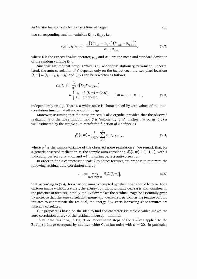
To validate this idea, in Fig. 3 we report some steps of the TV-flow applied to theBarbara image corrupted by additive white Gaussian noise with σ = 20. In particular,
286 R. H. Chan, A. Lanza, S. Morigi and F. Sgallari
(a) u(20) (b) u(80) (c) u(120) (d) u(180)
(a) r(20) (b) r(80) (c) r(120) (d) r(180)
(a)Öρr(20) (b)Öρr(80) (c)×ρr(120) (d)×ρr(180)Figure 3: Some steps of the TV-�ow applied to the Barbara image orrupted by a white Gaussiannoise with σ = 20 (�rst row); orresponding residual images (se ond row); orresponding sample auto- orrelation, restri ted to the smaller lags [l , m] : l , m= 0, 1, · · · , 9 (third row).in the first, second and third rows we show, respectively, the images filtered by the TV-
flow, u(k), the residual images, r(k) and a zoom of the auto-correlation function of the
residual images,Ôρr(k) , restricted to the smaller lags [l, m] : l, m = 0,1, · · · , 9. Moreover,
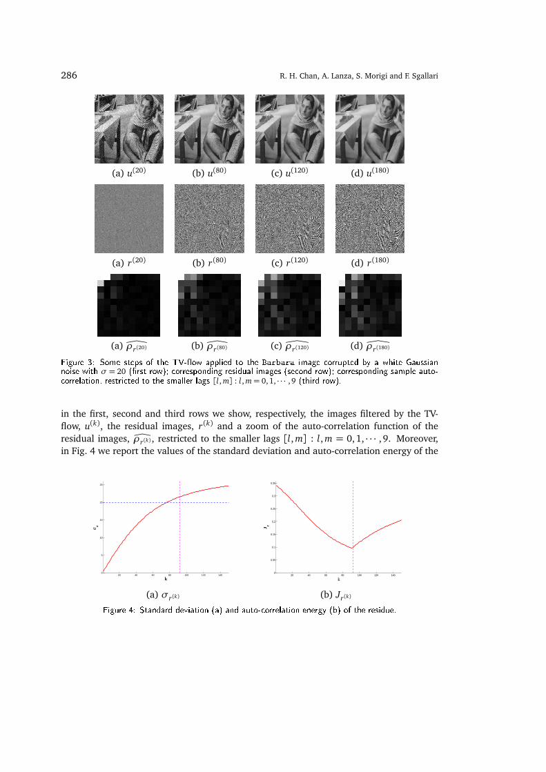
in Fig. 4 we report the values of the standard deviation and auto-correlation energy of the
20 40 60 80 100 120 1400
5
10
15
20
25
k
σ r
20 40 60 80 100 120 1400
0.05
0.1
0.15
0.2
0.25
0.3
0.35
k
J r
(a) σr(k) (b) Jr(k)Figure 4: Standard deviation (a) and auto- orrelation energy (b) of the residue.
An Adaptive Strategy for the Restoration of Textured Images 287
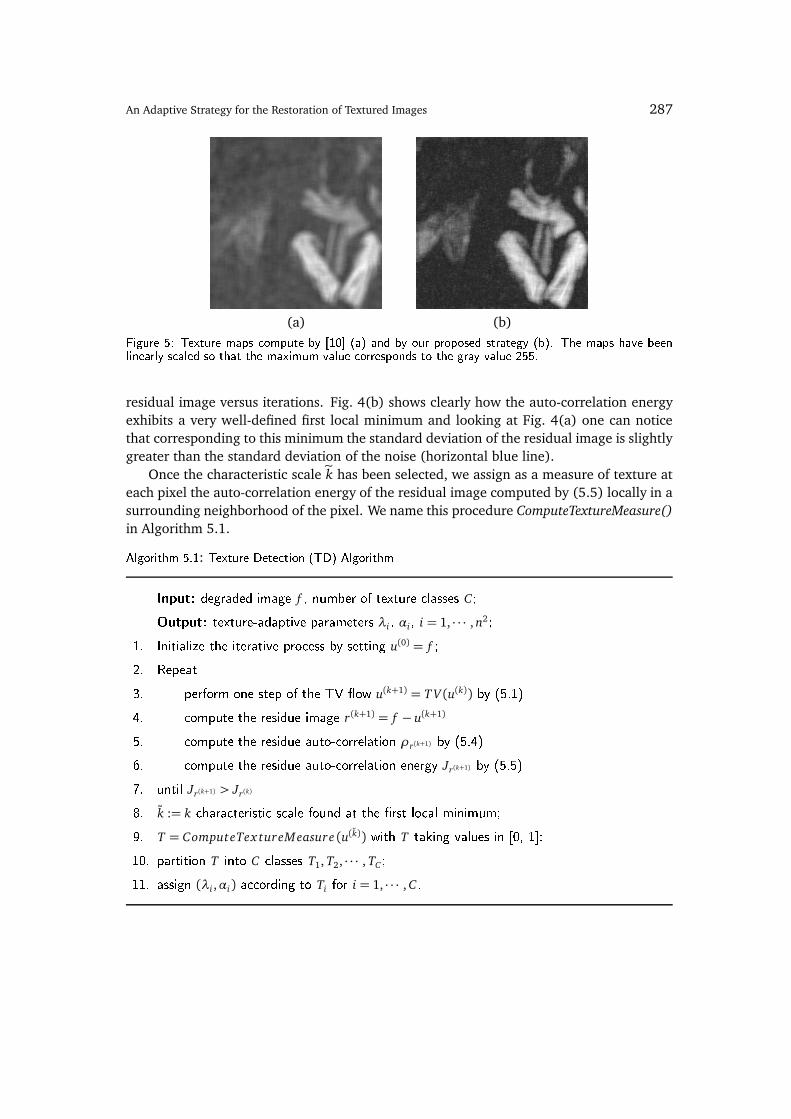
(a) (b)Figure 5: Texture maps ompute by [10℄ (a) and by our proposed strategy (b). The maps have beenlinearly s aled so that the maximum value orresponds to the gray value 255.residual image versus iterations. Fig. 4(b) shows clearly how the auto-correlation energy
exhibits a very well-defined first local minimum and looking at Fig. 4(a) one can notice
that corresponding to this minimum the standard deviation of the residual image is slightly
greater than the standard deviation of the noise (horizontal blue line).
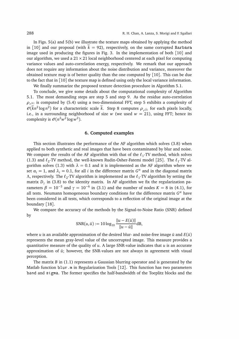
Once the characteristic scale ek has been selected, we assign as a measure of texture at
each pixel the auto-correlation energy of the residual image computed by (5.5) locally in a
surrounding neighborhood of the pixel. We name this procedure ComputeTextureMeasure()
in Algorithm 5.1.Algorithm 5.1: Texture Dete tion (TD) AlgorithmInput: degraded image f , number of texture lasses C;Output: texture-adaptive parameters λi, αi, i = 1, · · · , n2;1. Initialize the iterative pro ess by setting u(0) = f ;2. Repeat3. perform one step of the TV �ow u(k+1) = T V (u(k)) by (5.1)4. ompute the residue image r(k+1) = f − u(k+1)5. ompute the residue auto- orrelation ρr(k+1) by (5.4)6. ompute the residue auto- orrelation energy Jr(k+1) by (5.5)7. until Jr(k+1) > Jr(k)8. k := k hara teristi s ale found at the �rst lo al minimum;9. T = ComputeTex tureMeasure (u(k)) with T taking values in [0, 1℄;10. partition T into C lasses T1, T2, · · · , TC ;11. assign (λi ,αi) a ording to Ti for i = 1, · · · , C.
288 R. H. Chan, A. Lanza, S. Morigi and F. Sgallari
In Figs. 5(a) and 5(b) we illustrate the texture maps obtained by applying the method
in [10] and our proposal (with ek = 92), respectively, on the same corrupted Barbaraimage used in producing the figures in Fig. 3. In the implementation of both [10] and
our algorithm, we used a 21×21 local neighborhood centered at each pixel for computing
variance values and auto-correlation energy, respectively. We remark that our approach
does not require any information about the noise distribution and variance, moreover the
obtained texture map is of better quality than the one computed by [10]. This can be due
to the fact that in [10] the texture map is defined using only the local variance information.
We finally summarize the proposed texture detection procedure in Algorithm 5.1.
To conclude, we give some details about the computational complexity of Algorithm
5.1. The most demanding steps are step 5 and step 9. As the residue auto-correlation
ρr(k) is computed by (5.4) using a two-dimensional FFT, step 5 exhibits a complexity of
O (ekn2 log n2) for a characteristic scale ek. Step 8 computes ρr(ek) for each pixels locally,
i.e., in a surrounding neighborhood of size w (we used w = 21), using FFT; hence its
complexity is O (n2w2 log w2).
6. Computed examples
This section illustrates the performance of the AF algorithm which solves (3.8) when
applied to both synthetic and real images that have been contaminated by blur and noise.
We compare the results of the AF algorithm with that of the ℓ1-TV method, which solves
(1.3) and ℓ2-TV method, the well-known Rudin-Osher-Fatemi model [25]. The ℓ1-TV al-
gorithm solves (1.3) with λ = 0.1 and it is implemented as the AF algorithm where we
set αi = 1, and λi = 0.1, for all i in the difference matrix Gα and in the diagonal matrix
Λ, respectively. The ℓ2-TV algorithm is implemented as the ℓ1-TV algorithm by setting the
matrix Dγ in (3.8) to the identity matrix. In AF algorithm we fix the regularization pa-
rameters β = 10−3 and γ = 10−6 in (3.1) and the number of nodes K = 8 in (4.1), for
all tests. Neumann homogeneous boundary conditions for the difference matrix Gα have
been considered in all tests, which corresponds to a reflection of the original image at the
boundary [18].
We compare the accuracy of the methods by the Signal-to-Noise Ratio (SNR) defined
by
SNR(u, u) := 10 log10
‖u− E(u)‖
‖u− u‖dB,
where u is an available approximation of the desired blur- and noise-free image u and E(u)
represents the mean gray-level value of the uncorrupted image. This measure provides a
quantitative measure of the quality of u. A large SNR-value indicates that u is an accurate
approximation of u; however, the SNR-values are not always in agreement with visual
perception.
The matrix B in (1.1) represents a Gaussian blurring operator and is generated by the
Matlab function blur.m in Regularization Tools [12]. This function has two parametersband and sigma. The former specifies the half-bandwidth of the Toeplitz blocks and the
An Adaptive Strategy for the Restoration of Textured Images 289
latter the variance of the Gaussian point spread function. The larger sigma, the more
blurring. Enlarging band increases the storage requirement, the arithmetic work required
for the evaluation of matrix-vector products with B and to some extent the blurring.
The entries of f are contaminated either by additive Gaussian noise or by salt-and-
pepper noise. The noise is added to the blurred image to obtain the observed image f . In
the salt-and-pepper noise white and black pixels randomly occur, while unaffected pixels
always remain unchanged. The salt-and-pepper noise is usually quantified by the per-
centage of pixels which are corrupted. In the case of Gaussian noise, let ef ∈ Rn2
be the
associated vector with the unknown noise-free entries, i.e., f = ef + e where the vector e
represents the noise. We define the noise-level
ν =‖e‖
‖ef ‖(6.1)
in all the examples.
In these examples we partitioned the texture-map only into four classes, three texture
classes and one non-texture class, with associated fractional order and regularization pa-
rameter values α1 = 1.9, λ1 = 0.05, α2 = 1.8, λ2 = 0.05, α3 = 1.7, λ3 = 0.05 and
α4 = 1.0, λ4 = 1.0, respectively. For this particular case, the diagonal entries of the matrix
Λ may assume one of the four different values λ1, λ2, λ3 and λ4.
All computations are carried out in MATLAB with about 16 significant decimal digits.
As concerning the computational complexity of the AF algorithm, sketched in (3.1),
we have a preliminary texture detection step (see step 1 in (3.1)), whose complexity has
been discussed in Section 5. Then, the core of the algorithm consists of an outer iteration
loop (step 3 in (3.1)) and an inner iteration loop required by the iterative solver CG for
the linear system in (3.8). From our experience very good results are obtained by at
most 10 outer iterations, while the number of inner iterations depends on the required
tolerance. In our experiments we used 10−4 as stopping tolerance for the CG algorithm,
that involves an average of 18 inner iterations. Each iteration in the inner loop requires
the evaluation of one matrix-vector product with the matrix which is composed by the sum
of two matrices, one related to the regularizer and the other to the blur operator. The
implementation details of the former are given in Section 4, while the latter makes use of
FFT convolutions.
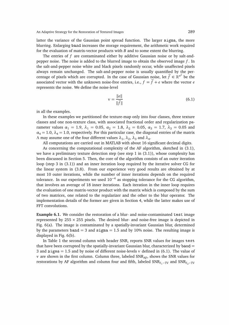
Example 6.1. We consider the restoration of a blur- and noise-contaminated test image
represented by 255× 255 pixels. The desired blur- and noise-free image is depicted in
Fig. 6(a). The image is contaminated by a spatially-invariant Gaussian blur, determined
by the parameters band = 3 and sigma = 1.5 and by 10% noise. The resulting image is
displayed in Fig. 6(b).
In Table 1 the second column with header SNRi reports SNR values for images testthat have been corrupted by the spatially-invariant Gaussian blur, characterized by band=3 and sigma = 1.5 and by noise of different noise-levels ν defined in (6.1). The value of
ν are shown in the first column. Column three, labeled SNRAF, shows the SNR values for
restorations by AF algorithm and column four and fifth, labeled SNRℓ1−TV and SNRℓ2−TV
290 R. H. Chan, A. Lanza, S. Morigi and F. Sgallari
(a) true image (b) observed image
(c) ℓ1-TV (d) AF
(e) ℓ2-TV (f) texture mapFigure 6: Example 6.1. test images: (a) blur- and noise-free image; (b) the orrupted image produ edby Gaussian blur, de�ned by the parameters band = 3 and sigma = 1.5 and by 10% of Gaussian noise;( ) restoration with ℓ1-TV with λ1 = 0.1; (d) restored image determined by AF algorithm; ( ) restorationwith ℓ2-TV with λ1 = 0.1; (f) texture lasses omputed on (b).show the SNR values for restorations by TV method, implemented by (1.3) with ℓ1 and ℓ2data fidelity terms, respectively.
The adaptive regularization process applies different levels of denoising in different
image regions. This improves the result visually, in terms of texture preservation and
smoothing of the homogeneous regions and in terms of signal-to noise-ratio. Fig. 6(d)
shows the restoration by AF algorithm and Fig. 6(f) depicts the texture-map used for the
restoration. The texture measures are obtained on the corrupted image in Fig. 6(b) and
the four texture classes are shown using gray-level values. In particular, in black regions
the AF algorithm is applied with α4 = 1.0, α2 = 1.7 and α3 = 1.8 in the gray regions
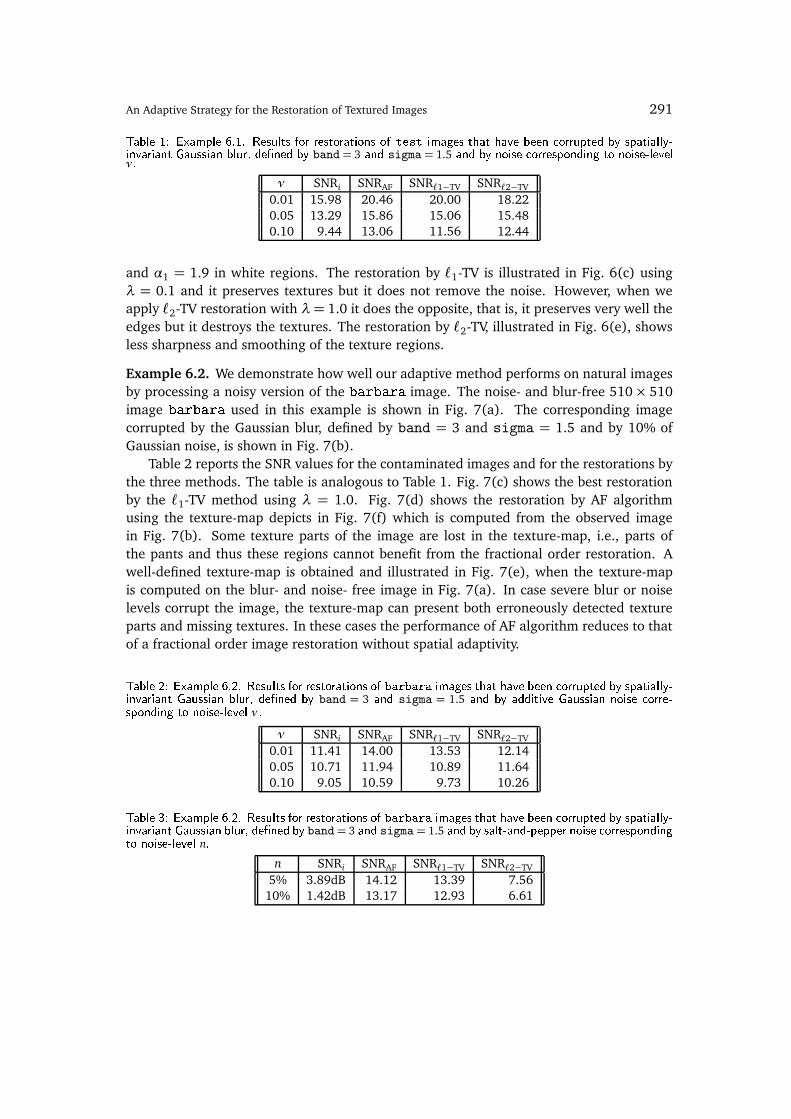
An Adaptive Strategy for the Restoration of Textured Images 291Table 1: Example 6.1. Results for restorations of test images that have been orrupted by spatially-invariant Gaussian blur, de�ned by band = 3 and sigma = 1.5 and by noise orresponding to noise-levelν .
ν SNRi SNRAF SNRℓ1−TV SNRℓ2−TV
0.01 15.98 20.46 20.00 18.22
0.05 13.29 15.86 15.06 15.48
0.10 9.44 13.06 11.56 12.44
and α1 = 1.9 in white regions. The restoration by ℓ1-TV is illustrated in Fig. 6(c) using
λ = 0.1 and it preserves textures but it does not remove the noise. However, when we
apply ℓ2-TV restoration with λ= 1.0 it does the opposite, that is, it preserves very well the
edges but it destroys the textures. The restoration by ℓ2-TV, illustrated in Fig. 6(e), shows
less sharpness and smoothing of the texture regions.
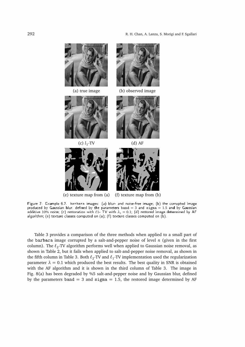
Example 6.2. We demonstrate how well our adaptive method performs on natural images
by processing a noisy version of the barbara image. The noise- and blur-free 510× 510
image barbara used in this example is shown in Fig. 7(a). The corresponding image
corrupted by the Gaussian blur, defined by band = 3 and sigma = 1.5 and by 10% of
Gaussian noise, is shown in Fig. 7(b).
Table 2 reports the SNR values for the contaminated images and for the restorations by
the three methods. The table is analogous to Table 1. Fig. 7(c) shows the best restoration
by the ℓ1-TV method using λ = 1.0. Fig. 7(d) shows the restoration by AF algorithm
using the texture-map depicts in Fig. 7(f) which is computed from the observed image
in Fig. 7(b). Some texture parts of the image are lost in the texture-map, i.e., parts of
the pants and thus these regions cannot benefit from the fractional order restoration. A
well-defined texture-map is obtained and illustrated in Fig. 7(e), when the texture-map
is computed on the blur- and noise- free image in Fig. 7(a). In case severe blur or noise
levels corrupt the image, the texture-map can present both erroneously detected texture
parts and missing textures. In these cases the performance of AF algorithm reduces to that
of a fractional order image restoration without spatial adaptivity.Table 2: Example 6.2. Results for restorations of barbara images that have been orrupted by spatially-invariant Gaussian blur, de�ned by band = 3 and sigma = 1.5 and by additive Gaussian noise orre-sponding to noise-level ν .ν SNRi SNRAF SNRℓ1−TV SNRℓ2−TV
0.01 11.41 14.00 13.53 12.14
0.05 10.71 11.94 10.89 11.64
0.10 9.05 10.59 9.73 10.26Table 3: Example 6.2. Results for restorations of barbara images that have been orrupted by spatially-invariant Gaussian blur, de�ned by band= 3 and sigma = 1.5 and by salt-and-pepper noise orrespondingto noise-level n.n SNRi SNRAF SNRℓ1−TV SNRℓ2−TV
5% 3.89dB 14.12 13.39 7.56
10% 1.42dB 13.17 12.93 6.61
292 R. H. Chan, A. Lanza, S. Morigi and F. Sgallari
(a) true image (b) observed image
(c) l1-TV (d) AF
(e) texture map from (a) (f) texture map from (b)Figure 7: Example 6.2. barbara images: (a) blur- and noise-free image; (b) the orrupted imageprodu ed by Gaussian blur, de�ned by the parameters band = 3 and sigma = 1.5 and by Gaussianadditive 10% noise; ( ) restoration with ℓ1- TV with λ1 = 0.1; (d) restored image determined by AFalgorithm; (e) texture lasses omputed on (a); (f) texture lasses omputed on (b).Table 3 provides a comparison of the three methods when applied to a small part of
the barbara image corrupted by a salt-and-pepper noise of level n (given in the first
column). The ℓ2-TV algorithm performs well when applied to Gaussian noise removal, as
shown in Table 2, but it fails when applied to salt-and-pepper noise removal, as shown in
the fifth column in Table 3. Both ℓ2-TV and ℓ1-TV implementation used the regularization
parameter λ = 0.1 which produced the best results. The best quality in SNR is obtained
with the AF algorithm and it is shown in the third column of Table 3. The image in
Fig. 8(a) has been degraded by %5 salt-and-pepper noise and by Gaussian blur, defined
by the parameters band = 3 and sigma = 1.5, the restored image determined by AF
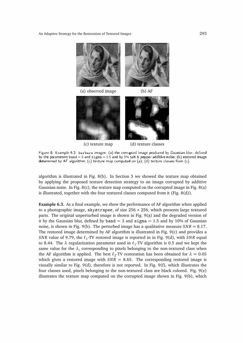
An Adaptive Strategy for the Restoration of Textured Images 293
(a) observed image (b) AF
(c) texture map (d) texture classesFigure 8: Example 6.2. barbara images: (a) the orrupted image produ ed by Gaussian blur, de�nedby the parameters band = 3 and sigma= 1.5 and by 5% salt & pepper additive noise; (b) restored imagedetermined by AF algorithm; ( ) texture map omputed on (a); (d) texture lasses from ( ).algorithm is illustrated in Fig. 8(b). In Section 5 we showed the texture map obtained
by applying the proposed texture detection strategy to an image corrupted by additive
Gaussian noise. In Fig. 8(c), the texture map computed on the corrupted image in Fig. 8(a)
is illustrated, together with the four textured classes computed from it (Fig. 8(d)).
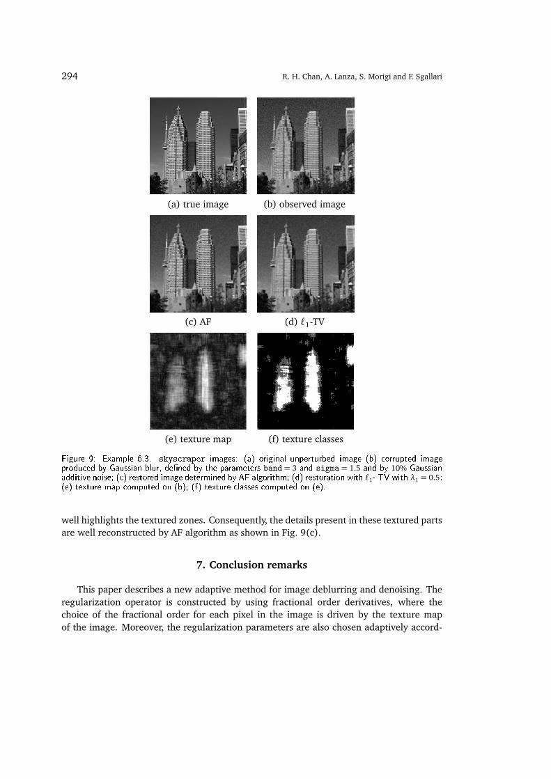
Example 6.3. As a final example, we show the performance of AF algorithm when applied
to a photographic image, skys raper, of size 256× 256, which presents large textured
parts. The original unperturbed image is shown in Fig. 9(a) and the degraded version of
it by the Gaussian blur, defined by band = 3 and sigma = 1.5 and by 10% of Gaussian
noise, is shown in Fig. 9(b). The perturbed image has a qualitative measure SNR = 8.17.
The restored image determined by AF algorithm is illustrated in Fig. 9(c) and provides a
SNR value of 9.79, the ℓ1-TV restored image is reported in in Fig. 9(d), with SNR equal
to 8.44. The λ regularization parameter used in ℓ1-TV algorithm is 0.5 and we kept the
same value for the λi corresponding to pixels belonging to the non-textured class when
the AF algorithm is applied. The best ℓ2-TV restoration has been obtained for λ = 0.05
which gives a restored image with SNR = 8.65. The corresponding restored image is
visually similar to Fig. 9(d), therefore is not reported. In Fig. 9(f), which illustrates the
four classes used, pixels belonging to the non-textured class are black colored. Fig. 9(e)
illustrates the texture map computed on the corrupted image shown in Fig. 9(b), which
294 R. H. Chan, A. Lanza, S. Morigi and F. Sgallari
(a) true image (b) observed image
(c) AF (d) ℓ1-TV
(e) texture map (f) texture classesFigure 9: Example 6.3. skys raper images: (a) original unperturbed image (b) orrupted imageprodu ed by Gaussian blur, de�ned by the parameters band= 3 and sigma= 1.5 and by 10% Gaussianadditive noise; ( ) restored image determined by AF algorithm; (d) restoration with ℓ1- TV with λ1 = 0.5;(e) texture map omputed on (b); (f) texture lasses omputed on (e).well highlights the textured zones. Consequently, the details present in these textured parts
are well reconstructed by AF algorithm as shown in Fig. 9(c).
7. Conclusion remarks
This paper describes a new adaptive method for image deblurring and denoising. The
regularization operator is constructed by using fractional order derivatives, where the
choice of the fractional order for each pixel in the image is driven by the texture map
of the image. Moreover, the regularization parameters are also chosen adaptively accord-
An Adaptive Strategy for the Restoration of Textured Images 295
ing to the texture map. This makes the proposed algorithm an efficient tool to preserve
texture well in the texture regions while removing noise and staircase effects in the image.
We have developed a simple iterative algorithm to solve the model which is based on the
half-quadratic strategy. Numerical results showed that the proposed algorithm yields bet-
ter signal-to-noise ratio and visual effects than using non-adaptive fractional order image
restorations based on TV regularization and ℓ1 or ℓ2 data fitting terms.
Increasing the number of texture classes would maintain the same computational cost
of the AF algorithm while improving the accuracy in terms of SNR value. We will investi-
gate this important aspect in future experiments.
Acknowledgments This work has been partially supported by MIUR-Prin 2008, ex60%
project by University of Bologna "Funds for selected research topics" and by GNCS-INDAM.
References
[1] J. O. ABAD, S. MORIGI, L. REICHEL AND F. SGALLARI, Alternating Krylov subspace image restora-
tion methods, JCAM, 236(8) (2012), pp. 2049–2062.
[2] J. BAI AND X. C. FENG, Fractional-order anisotropic diffusion for image denoising, IEEE Trans.
Image Process., 16(10) (2007), pp. 2492–2502.
[3] D. BERTACCINI, R. H. CHAN, S. MORIGI AND F. SGALLARI, An adaptive norm algorithm for image
restoration, A. M. Bruckstein et al. (Eds.): SSVM 2011, LNCS 6667, pp. 194–205, Springer-
Verlag Berlin Heidelberg, 2011.
[4] A. BUADES, B. COLL AND J.-M. MOREL, A non-local algorithm for image denoising, IEEE Int.
Conf. Computer Vision and Pattern Recognition (CVPR 2005), San Diego, CA, USA, 2005.
[5] T. CHAN AND S. ESEDOGLU, Aspects of total variation regularized L1 function approximation,
SIAM J. Appl. Math., 65 (2005), pp. 1817–1837.
[6] R. H. CHAN AND H. X. LIANG, A fast and efficient half-quadratic algorithm for TV-L1 image
restoration, CHKU research report 370, 2010, submitted; available at ftp://ftp.math. uhk.edu.hk/report/2010-03.ps.Z.
[7] T. F. CHAN, S. OSHER AND J. SHEN, The digital TV filter and nonlinear denoising, IEEE Trans.
Image Process., 10(2) (2001) pp. 231–241.
[8] H. FARID, Discrete-Time Fractional Differentiation from Integer Derivatives, TR2004-528, De-
partment of Computer Science, Dartmouth College, 2004.
[9] D. GEMAN AND C. YANG, Nonlinear image recovery with half-quadratic regularization and FFTs,
IEEE Trans. Image Proc., 4 (1995), pp. 932–946.
[10] G. GILBOA, Y. Y. ZEEVI AND N. SOCHEN, Texture preserving variational denoising using adaptive
fidelity term, Proc. Variational and Level-Set Methods 2003, Nice, France, pp. 137–144, 2003.
[11] P. C. HANSEN, Rank-deficient and discrete ill-posed problems, SIAM, 1998.
[12] P. C. HANSEN, Regularization tools: a Matlab package for analysis and solution of discrete ill-
posed problems, Numer. Algorithms, 6 (1994), pp. 1–35.
[13] P. C. HANSEN, J. G. NAGY AND D. P. O’LEARY, Deblurring Images: Matrices, Spectra and Filter-
ing, SIAM, Philadelphia, 2006.
[14] Y. LI AND F. SANTOSA, A computational algorithm for minimizing total variation in image restora-
tion, IEEE Trans. Image Process., 5(6) (1996), pp. 987–995.
[15] M. LYSAKER, A. LUNDERVOLD AND X. C. TAI, Noise removal using fourth-order partial differential
equation with applications to medical magnetic resonance images in space and time, IEEE Trans.
Image Process., 12(12) (2003), pp. 1579–1590.

296 R. H. Chan, A. Lanza, S. Morigi and F. Sgallari
[16] S. MORIGI, L. REICHEL, F. SGALLARI AND A. SHYSHKOV, Cascadic multiresolution methods for
image deblurring, SIAM J. Imaging Sci., 1 (2008), pp. 51–74.
[17] M. K. NG, H. SHEN, E. Y. LAM AND L. ZHANG, A total variation regularization based super-
resolution reconstruction algorithm for digital video, EURASIP J. Advances Signal Proces., vol.
2007, Article ID 74585 (2007).
[18] M. K. NG, R. H. CHAN AND W.-C. TANG, A fast algorithm for deblurring models with Neumann
boundary conditions, SIAM J. Sci. Comput., 21 (1999), pp. 851–866.
[19] M. NIKOLOVA AND R. CHAN, The equivalence of half-quadratic minimization and the gradient
linearization iteration, IEEE Trans. Image Proc., 16 (2007), pp. 1623–1627.
[20] M. NIKOLOVA, A variational approach to remove outliers and impulse noise, J. Math. Imaging
Vision, 20(1-2) (2004), pp. 99–120.
[21] M. ORTIGUEIRA, A coherent approach to non integer order derivatives, Signal Process., 86
(2006), pp. 2505-2515.
[22] P. PERONA AND J. MALIK, Scale-space and edge detection using anisotropic diffusion, IEEE Trans.
Pattern Anal. Mach. Intell., 12 (1990), pp. 629–639.
[23] I. PODLUBNY, Fractional Differential Equations, Academic Press, New York, 1999.
[24] I. PODLUBNY, A. CHECHKIN, T. SKOVRANEK, Y. CHEN AND B. M. V. JARA, Matrix approach to discrete
fractional calculus II: partial fractional differential equations, J. Comput. Phys., 228(8) (2009),
pp. 3137–3153.
[25] L. RUDIN, S. OSHER AND E. FATEMI, Nonlinear total variation based noise removal algorithms,
Phys. D, 60 (1992), pp. 259–268.
[26] C. WU, J. ZHANG AND X. TAI, Augmented Lagrangian method for total variation restoration with
non-quadratic fidelity, UCLA CAM Report 09-82, 2009.
[27] J. YANG, Y. ZHANG AND W. YIN, An efficient TVL1 algorithm for deblurring multichannel images
corrupted by impulsive noise, SIAM J. Sci. Comput., 31 (2009), pp. 2842–2865.
[28] W. YIN, D. GOLDFARB AND S. OSHER, Image cartoon-texture decomposition and feature selec-
tion using the total variation regularized L1 functional, in Variational, Geometric and Level Set
Methods in Computer Vision, Lecture Notes in Computer Science, 3752, pp. 73–74, Springer,
2005.
[29] W. YIN, D. GOLDFARB AND S. OSHER, The total variation regularized L1 model for multiscale
decomposition, Multiscale Model. Simul., 6 (2006), pp. 190–211.
[30] J. ZHANG AND Z. WEI, Fractional variational model and algorithm for image denoising, Proceed.
Fourth International conference on Natural Computation, IEEE, 2008.
[31] J. ZHANG, Z. WEI AND L. XIAO, Adaptive fractional-order multi-scale method for image denoising,
J. Math. Imaging Vision, 43(1) (2012), pp. 39–49.
[32] J. ZHANG AND Z. WEI, A class of fractional-order multi-scale variational models and alternating
projection algorithm for image denoising, Appl. Math. Modelling, 35(5) (2011), pp. 2516–
2528.