applied sciences

Article

An Accurate Probabilistic Model for TVWS Identification

Danilo Corral-De-Witt 1,2,* , Sabbir Ahmed 1 , Faroq Awin 1,3 , José Luis Rojo-Álvarez 4 andKemal Tepe 1

1 Department of Electrical and Computer Engineering, University of Windsor, Windsor, ON N9B 3P4, Canada;sabbir.ahmed@uwindsor.ca (S.A.); awin@uwindsor.ca (F.A.); ktepe@uwindsor.ca (K.T.)

2 Departamento de Eléctrica y Electrónica, Universidad de las Fuerzas Armadas ESPE,Sangolquí 171103, Ecuador

3 Department of Electrical and Electronic Engineering, University of Tripoli, Tripoli 13555, Libya4 Departamento de Teoría de la Señal y Comunicaciones, Sistemas Telemáticos y Computación, Universidad

Rey Juan Carlos, 28933 Móstoles, Spain; joseluis.rojo@urjc.es* Correspondence: corraldd@uwindsor.ca; Tel.: +1-226-246-5278

Received: 16 September 2019; Accepted: 5 October 2019; Published: 10 October 2019

Abstract: Television White Spaces (TVWS)-based cognitive radio systems can improve spectrumefficiency by facilitating opportunistic usage of television broadcasting spectrum by secondary userswithout interfering with primary users. Previously applied models introduce missed detection errors,giving a limited estimation of the spectrum occupancy, which does not correspond to the realityof its usage, hence resulting in a partial waste of this resource. Considering jointly parameterslike false alarm probability and detection probability, this article proposes a probabilistic modelthat can identify TVWS with improved accuracy. The proposed model considers energy detectioncriteria, combined with simultaneous sensing of the noise and of the signal from primary users.In order to demonstrate the model effectiveness, a low-cost Mobile Spectrum Sensing Stationprototype was designed, implemented, and subsequently mounted on a vehicle. More than eightmillion spatio-temporally variant data samples were collected by scanning the UHF-TV spectrumof 500–698 MHz in the city of Windsor, ON, Canada. Analysis of the collected data showed thatthe proposed model achieves an accuracy improvement of about 9.6% compared to existing models,demonstrating that TVWS vary with spatial displacement and increasing significantly in the ruralareas. Even in the most crowded spectrum zone, about 28% of the channels are identified as TVWS,and this number increases to a maximum of 60% in less crowded regions in urban areas. We concludethat the proposed model improves the TVWS detection compared with other used models, and alsothat the elements considered in this research contribute to reduce the complexity of the mathematicalcalculations while maintaining the accuracy. A low-cost open-source sensing station has beendesigned and tested, which represents an operative and useful data source in this setting.

Keywords: TVWS; dynamic spectrum access; false alarm probability; detection probability

1. Introduction

Technologies for data-centric wireless communications have experienced an incredibledevelopment in the last decade, resulting in huge demands for electromagnetic spectrum.Present spectrum scenarios show a peculiar characteristic, as some bands of the spectrum are extremelycrowded, whereas some others are underused. Thus, there is scarcity as well as wastage [1,2].Smart sharing of the spectrum appears to be a promising solution to this problem. The use of CognitiveRadio (CR) with different sensing techniques allows us to detect unused channels, known as WhiteSpaces (WS), for their opportunistic usage by Secondary Users (SU) without affecting the Primary Users(PU), through a process called Dynamic Spectrum Access (DSA) [3]. In this context, Television White

Appl. Sci. 2019, 9, 4232; doi:10.3390/app9204232 www.mdpi.com/journal/applsci

Appl. Sci. 2019, 9, 4232 2 of 25

Spaces (TVWS) are of special interest and this increasingly used term refers to WS that are locatedin any of the bands assigned to TV-broadcasting service bands [4]. TV spectrum bands often showunderutilization by PU and hence the use of TVWS in CR is a promising solution to spectrum scarcity.In this setting, the Institute of Electrical and Electronics Engineers (IEEE) approved the 802.22 standardin 2011 [5]. It is important to note that independently of which spectrum band is being used, CR mustavoid interference with PU at any time. But even before that, the task of finding a model that allowsaccurate identification of TVWS minimizing false alarms errors needs attention.

In this article, we propose an accurate statistical model to identify the presence of TVWS basedon the False Alarm Probability (Pf a) and on the Detection Probability (Pd). These parameters areobtained by simultaneous sensing the noise intensity (W( f )) and the signal of the PU (X( f )) in theenvironmental spectrum. The functional block diagram representing the system that correspondsto our proposed model is shown in Figure 1. As observed, W( f ) and X( f ) are the two inputsto the collection block where data processing takes place. Next, the processed data is fed to theanalysis block, where all the stochastic and mathematical analyses are performed. Then followsthe decision block, where the presence or absence of the PU is decided. Finally, results are visuallydemonstrated in the results block. As finally concluded, this model gives about 9.6% increase in Pdcompared to other existing models. The motivation behind undertaking this research endeavouris the fact that CR TVWS has a huge potential in many diverse wireless services and applications,for example, internet access for rural areas, Wireless Regional Area Networks (WRAN), Wireless SensorNetworks (WSN), Emergency Communications (EC), and Telecommunications for Disaster Relief(TDR), among many others. Particularly, the last two applications (i.e., EC and TDR) have drawnsignificant research interest as they are both related to rescuing lives.

The rest of the manuscript is organized as follows. Section 2 provides a review of the backgroundfor this research. Section 3 is a description of the used hardware and data collection patterns. Section 4describes the proposed model and the mechanism to find TVWS. Experimental results are shown anddiscussed in Section 5. Conclusions are presented in Section 6.

Figure 1. Block diagram of the proposed model.

2. Background

The term CR was coined by Joseph Mitola in his 1999 work [6]. The author described thereinhow CR could enhance the flexibility of personal wireless services through the so-called RadioKnowledge Representation Language (RKRL). CR is often described as a “disruptive, but unobtrusivetechnology” [7]. It is disruptive because it allows a SU to access the PU bands, and it is unobtrusivedue to the control of different parameters, such as access or transmission power, which dramaticallyreduces any harmful interference with the PU.

Looking at the current spectrum scenario, we find that the use of unlicensed bands are seen almosteverywhere, especially because of the numerous services available to hand-held wireless devices,including Industrial, Scientific, and Medical (ISM) band at 2.4 GHz and the National InformationInfrastructure (U-NII) band at 5.2 GHz. This is actually a reflection of how much today’s society isdependent on wireless spectrum [8]. To access and use these open bands, the user does not need to payany fee or to ask for a license with the local regulator, and more, these bands have similar counterpartsaround the world, with international regulatory bodies working to align bands and regulations [9].

Appl. Sci. 2019, 9, 4232 3 of 25

The common use of unlicensed bands and the development of new devices and technologies ledregulatory bodies like the FCC to consider opening further bands for unlicensed use. As stated by theJournal of Communications, “Whereas, spectrum occupancy measurements show that licensed bands, such asthe TV bands, are significantly underutilized” [8]. In simple words, what CR is allowing an unlicenseduser is to use licensed bands in the very same manner the user would use unlicensed bands, i.e., no feeor no license required. As an alternative to using unlicensed bands, CR is considered the solution tothe spectrum wastage due to low usage of the licensed radio spectrum [7]. This technology workson the principle of adapting the operating parameters of the radio according to the conditions of theenvironment. Thereby it facilitates smart, efficient, and reliable spectrum usage through identifyingand exploiting a large amount of unused or underused spectrum bands.

In May 2004, the Federal Communications Commission (FCC) of the United States, proposed thecreation of the 802.22 workgroup (WG) for Wireless Regional Area Networks (WRAN). The WG’s goalwas to develop the PHY and MAC air interfaces to allow unlicensed users or SUs to operate in theTV broadcast bands without interfering with the PU [10]. During this time, researchers developedspectrum sensing techniques and simulation models, and the idea of smart spectrum gained muchinterest [5,11]. In 2011, the IEEE 802.22 WRAN standard was approved, which defined a worldwidestandard air interface based on CR techniques for the TV broadcasting band [8,12]. Following theseguidelines, researchers are considering nowadays different methods to identify idle channel withinTV bands or in general within any band. In [13], a detailed list is given with works that use differentparameters to identify occupied vs. available channels. These include, for example, statistics withpower detection, occupation and duty cycle, Probability Density Function (pdf) or Cumulative DensityFunction (CDF) with power detection, Markov chains, linear regression, and spectrum prediction,among others. In [14], the authors proposed a spectrum scanning method based on Bayesian inferenceto estimate the channel occupancy rate, by considering the false alarm and detection probabilities.This approach showed better accuracy compared to other works considering only energy detection todefine the presence or absence of a PU.

Based on our analysis of the above mentioned works, we propose that at least three parametersshould be considered in each geographical location to evaluate a TV channel, namely, the realinstantaneous noise signal, the composite signal consisting of users’ signal and noise, and the energydetected in each reading. These parameters ensure the accuracy of the detected channels and can beused to apply or adapt the IEEE 802.22 standard in current CR systems.

2.1. Cognitive Radio Fundamentals

The functionalities of CR [15] are the following. First, spectrum sensing refers to identify theavailable spectrum channels and detect the presence of PU operating in a licensed band. Second,spectrum management is the possibility to select the best available channel from all the idle channelsdetected. Third, spectrum sharing refers to coordinate the smart access to a channel assigned to a PUwhen it is unused. Fourth, spectrum mobility is the option to vacate the channel when a PU is detected.

According to the definition given by the FCC, A Cognitive Radio is a radio that can change itstransmitter parameters based on interaction with the environment in which it operates [16]. From thisdefinition, CR has two characteristics, namely, cognitivity and reconfigurability. Cognitivity is thepossibility of the device to sense the spectrum. This is not the simple monitoring of the power in adetermined frequency band, but rather it requires more elements to identify the temporal and spatialvariations in the radio environment, all the time avoiding harmful interference to PU or to anotherSU. With this, it is possible to identify the unused channels or WS at a specific time or geographicallocation, giving the possibility to select the best operational parameters [7]. Reconfigurability is thecapability that permits a dynamic reconfiguration of the operational parameters according to the radioenvironment. In other words, CR devices can transmit and receive on a variety of frequencies withdifferent access technologies, thanks to their dynamic hardware features [17].

Appl. Sci. 2019, 9, 4232 4 of 25

The cycle of the CR is depicted in Figure 2. A portion of the spectrum in a time period ti isrepresented, with the signals of the PUs in orange, and the TVWS in white. The first step consists insensing the spectrum, then this information is analyzed, and based on the obtained result, the devicedecides which TVWS is the best option to transmit its information. This research is focused on thespectrum sensing and spectrum analysis stages of the CR cycle, specifically in the composite signalthat contains the PU information.

Figure 2. In the Cognitive Radio (CR) cycle, the UHF-TV spectrum band is sensed, then subsequentlyanalyzed, and a decision is taken based on the presence or absence of Primary Users (PUs).

2.2. TVWS Basics

As mentioned before, the unused and underutilized frequency spectrum spaces are referredto as WS. Efficient utilization of these WS has the potential to reduce the spectrum scarcity facednowadays with the fast growth of wireless technologies. According to [18], the characteristics of theWS are: (i) A white space is an unused radio frequency; (ii) Its existence depends on time, frequency,and geographical location; (iii) Its utilization should not cause any harm to the PU. These concepts areknown as TVWS when applied to the TV broadcasting frequencies.

In this research, we are interested in the frequency bands assigned to the TV service. Table 1illustrates the frequency ranges, channel numbers, bandwidth for each band, and the respective ITUregions [19] were the bands are allocated. Our work focuses on bands IV and V, i.e., 500 MHz to698 MHz [20,21]. It should be noted that channel 37 (608 MHz to 614 MHz) is used for radio astronomyand it is excluded from TV broadcast services. The three main reasons to choose said spectrum bandsare explained next. First, the propagation characteristics of frequencies under 1 GHz are favorablefor robust transmission, and there are standards as IEEE 802.22 considering the TV band to accessas a SU. Being recommended by an organization like IEEE, regulatory bodies across the globe havestarted applying them in their territories [5]. Second, the selected range of frequencies offers 198 MHz(32 channels) of continuous spectrum, except for channel 37. This spectral continuity gives morepossibilities to find and use idle channels without major modifications in the transmission parametersof the antennas. Third, multiple studies have demonstrated that there is a significant number ofunderused TV spectrum bands even in urban areas, and their availability increases rapidly in ruralareas [18].

Appl. Sci. 2019, 9, 4232 5 of 25

Table 1. Bands assigned to the TV broadcasting service, and their corresponding frequencies,channel numbers, partial Bandwidth (BW), and ITU regions.

Name Frequencies Channels Partial BW ITU Regions

Band I 54–72 2 to 4 18 MHz R1, R2, R3Band I (Cont.) 76–88 5 to 6 12 MHz R2

Band III 174–216 7 to 13 42 MHz R1, R2, R3Band IV 500–644 19 to 42 144 MHz R1, R2, R3Band V 644–698 43 to 51 54 MHz R1, R2, R3

3. Prototype Description

Before describing the prototype and its hardware configuration, it is necessary to review theproposed model. Six blocks are visualized in Figure 3, starting with block 1© that refers to sensing theinformation of the composite signal X( f ) and the noise signal W( f ) in a separate manner. Block 2©refers to how the samples obtained are processed by each device, i.e., the RF Explorer (RFE) and theSpectrum Analyzer (SA). In block 3©, the statistical parameters of each sensed signal are calculated andsaved. Block 4© shows the calculated Pf a, Pd, Missed-detection Probability (Pm), the optimum valuesfor Margin (M), and Threshold (T), and other information needed to analyze the UHF-TV spectrum.Block 5© features the Energy Detection (ED) procedure to identify unused channels and PU’s presence.Finally, block 6© explains how the output information is represented, detailing the amount of TVWS.Based on this model, the prototype must consider the elements listed in Table 2.

Figure 3. Chart flow of the proposed model.

Table 2. Hardware measurement setup of mobile spectrum sensing station.

Ord Device Observation

1 External Antenna Omni, 5 MHz to 1000 MHz range2 GPS Antenna USB connector3 Attached Impedance 50 Ω4 RF Explorer Sub 1 G, 240 MHz to 960 MHz range5 Spectrum Analyzer High accuracy, 50 KHz–3 GHz6 Portable Computer Hardware and software needed7 External Hard Disk To save readings and information

We designed a Mobile Spectrum Sensing Station (M-SSS) to measure TVWS over the UHF-TVspectrum in the city of Windsor and surroundings. Figure 4a shows that the M-SSS is composed of twoData Acquisition Instruments (DAI), in this case, two RFE installed in parallel, one device connectedto a Winegard antenna to collect information of the composite signal X( f ) and the other device with a50 Ω impedance attached and used to sense the noise of the system W( f ). These devices are employedto detect the energy of TV signals over the UHF band. This mobile configuration also has attached aGPS antenna to collect the geographical location for each reading.

The M-SSS was designed to be mounted on a vehicle. For this, a supporting structure wasassembled using a plastic pipe that fits in a Dodge Grand Caravan vehicle, as shown in Figure 4b–d.

Appl. Sci. 2019, 9, 4232 6 of 25

The antenna and the designed structure, support a speed up to 120 Km/h, verified, and theoretically,a speed up to 144 Km/h, according to data provided by the manufacturer.

(a) (b)

(c) (d)

Figure 4. Mobile Spectrum Sensing Station (M-SSS) designed to be mounted on a vehicle and sense theTV spectrum in wide geographical areas: (a) Diagram of the M-SSS; (b) Mounted station; (c) Winegardand GPS antennas; (d) M-SSS in operation.

We used two antennas in our system, a Winegard antenna, model MS-3005 VHF/UHF, 14.9′, and aGlobal Sat BU-353-S4 USB low consumption GPS antenna. The Winegard MS-3005 is an omnidirectionalantenna for receiving VHF and UHF-TV channels. Its frequency range is from 5 MHz to 1000 MHz.It can be installed in indoor or outdoor environments, and we used it to collect information with thedeigned M-SSS. Two Winegard antennas were used in this research, one installed on the laboratoryroof and another in the M-SSS, both aimed to collect information of the UHF-TV spectrum. The GPSinformation was collected with a BU-353-S4, which is a low power consumption device enclosed in acompact magnetic body, and it can be placed on the vehicle to receive the information of the Global-Satconstellation GPS satellites and save it in our Database (DB).

The RFE Sub1G device is a low cost, open source, and portable spectrum analyzer designed forthe specific needs of digital radio frequency communication. It supports the detection of expectedtransmission power, automatic resolution of Resolution Bandwidth (RBW), sweep time, and spectrumdata calculations. Moreover, it also has the features of real-time or adjusted signals, 3D spectrogramwaterfall, CSV export, and high-quality graphics. A large number of feature sets can be appliedand controlled through cooperated work between the RFE and Windows on the Personal Computer(PC) [22]. Two of these RFE devices were used in the M-SSS, one to collect noise samples and another tosense the composite signals, and both readings were sensed in each location. Its technical characteristicsare the following:

• Frequency Range 240 MHz to 960 MHz.• Span 0.112 MHz to 300 MHz.• Frequency Resolution 1 KHz.

Appl. Sci. 2019, 9, 4232 7 of 25

• Average Noise Level −115 dBm.• Amplitude Resolution 0.5 dBm.• Automatic RBW 2.6 KHz to 600 KHz.

The Tektronix MD04054-3 SA was used in this project, with the purpose of verifying the accuracyand quality of the readings taken with the RFE, and visualizing the obtained data. It is an oscilloscopewith a built-in spectrum analyzer [23], allowing to capture time-correlated analog, digital, and RFsignals. Its technical characteristics are:

• Frequency Range 50 KHz to 3 GHz.• Bandwidth 500 MHz.• Span 1 KHz to 3 GHz.• Frequency Resolution 20 Hz to 10 MHz.• Average Noise Level −115 dBm.• Amplitude Resolution 0.5 dBm.• Automatic RBW 2.6 KHz to 600 KHz.

By using the M-SSS, we measured the power level of the UHF-TV spectrum in the city of Windsor,following four trajectories. The samples were taken continuously along the sensed area. The RFEdevice scans 198 MHz bandwidth of the 500 MHz to 698 MHz UHF-TV spectrum with a separation of1.76 MHz at a given time instance. This means that there are 198 MHz/1.76 MHz = 112 samples readingper RFE at a given time instance. Along with two RFE devices, we used one GPS device. Hence, a singlereading constitutes of 112 Signal power in dBm, 112 Noise power in dBm, and 1 location-timestampdata samples. The RFE devices took readings every 0.340s which implies that for a duration of 1 minute,we had (112 + 112 + 1)× (60/0.34) = 39,705 data samples. The relevant data collection setup parametersare listed in Table 3, which shows that there are 36,176 readings representing 4,051,712 samples perRFE. Since there are 112 samples per reading, in total 8,103,424 samples were collected. The timeinterval between each reading was 0.340 seconds. The signal and noise data samples, along with theGPS information of Latitude and Longitude, were saved in the DB of the M-SSS.

Table 3. Number of readings and samples collected with each RF Explorer (RFE).

Trajectory Distance in Km Readings Noise Samples Signal Samples

T1 16.05 5417 612,752 612,752T2 32.45 10,419 1,166,928 1,166,928T3 31.48 12,924 1,447,488 1,447,488T4 23.22 7362 824,544 824,544

Total 103.20 36,176 4,051,712 4,051,712

4. Proposed Probabilistic Model

This section provides a brief explanation of the probabilistic model developed to address theresearch objectives. We start by analyzing how to calculate the reference noise level. Then a briefreview of M and T proposed by other authors, together with the parameters considered to calculateT, are detailed. The normality of the used distributions and the applicable tests are also included.Then, attention is paid to obtaining the pdf from the collected data, the used performance metrics,how to calculate Pf a and Pd, their maximum and minimum values, and how these values are relatedamong them.

4.1. Sensing the TV Signal and the Noise

The existence of the PU can be modeled by using the following hypotheses in thefrequency domain:

Appl. Sci. 2019, 9, 4232 8 of 25

H0 : X( f ) = W( f ) (1)

H1 : X( f ) = S( f ) + W( f ) (2)

where W( f ) denotes Additive White Gaussian Noise (AWGN), S( f ) denotes the received signal of thePU, X( f ) denotes the sensed composite of signal and noise, and H0 represents the null hypothesis forthe of PU absence in the channel, whereas H1 represents alternative hypothesis of the PU presence inthe channel.

By using the designed M-SSS, the information from the UHF-TV spectrum was collected at eachinstance of time ti and plotted, as shown by the example in Figure 5. In both cases, for RFE and forSA, the signal presents a similar shape in general terms, with specific frequencies in which the powerin dBm rises to its maximum values and other frequencies in which minimum values are reached.These panels show the power variations and differences between them in the time domain, which aredue to the internal characteristics of each device.

The information of X( f ) alone is not enough to identify TVWS, so that is imperative to find moreparameters allowing to identify the presence of PU. A crucial point to be considered is how the noiseis measured and its mean W( f ) is calculated. In the reviewed literature, in some cases, the noise issensed at the beginning of the measurement campaign and that value is used to be compared withall the readings, in other cases a theoretical value is considered, and a third approach is to considera fixed threshold T. In practice, it is very difficult to obtain accurate information about the noisepower [24] due to its variability or unexpected noise sources along the measured pattern when thesamples are taken.

According to the IEEE 802.22 standard [5,10], the channel in operation must be sensed severaltimes, namely, during the transmission, inter-framing time intervals, and in-framing. it is important toobtain trustful and accurate channel noise and signal samples. In order to obtain accurate informationregarding the noise, simultaneous sensing of the noise and the signal is here proposed. As it can beseen in Figure 4a, signal X( f ) is received through the antenna and sensed with one DAI, and at thesame time, another DAI with similar characteristics and a 50 Ω matched impedance is used to sensethe noise of the system. As a result, both the signals (i.e., X( f ) and W( f )) are used in our proposedchannel sensing mechanism.

With the mentioned hardware configuration, the UHF-TV spectrum was sensed, andrepresentative examples are shown in Figure 5a,c for the overlapped curves of W( f ) in blue andX( f ) in red, taken with the RFE and SA, respectively. The next logical step is to calculate the statisticalmean of the noise W( f ) in black, taken with the same instruments at time instant ti. Note that this isthe reference level for calculating T.

(a) (b)

(c) (d)

Figure 5. TV signals sensed with RFE (top) and SA (bottom) are compared. The X( f ) in red, W( f ) inblue, and W( f ) in black are observed in panels (a,c), W( f ) is the calculated noise level. In panels (b,d)are plotted X( f ), W( f ), and the different values for M or T.

Appl. Sci. 2019, 9, 4232 9 of 25

4.2. Threshold Considerations

As found in the literature of TVWS sensing, the sensed signal X( f ) is compared with ThresholdT, which is obtained from

T = W( f ) + M (3)

where W( f ) is the average noise floor level in dBm, and M is a margin in dB. Determining a thresholdplays a critical role in classifying PU activities as a busy or as an idle channel, i.e., TVWS [13]. Moreover,it is used to determine the duty cycle of the channel which defined as a ratio of the number of sensingsamples above the threshold to the total employed sensing samples. Generally, threshold is defined asan average noise floor level plus some margin. Different existing measurement campaigns conductedby other authors, have employed various margin values such as 5 dB in [25], 7 dB in [26], and ITU uses a10 dB, while the measurement in campaign [27], considered a fixed threshold of =−78 dBm. The mainreason of considering the margin is samples of noise measurement are not Gaussian distributed,therefore, adding margin excludes a wrong decision of PU existence by not considering noise as aPU signal [25]. In other words, noise samples cannot reach the threshold when adding margin tothe average noise floor level, therefore, false alarm will be reduced as only a PU signal can exceed it.However, such thresholds prevent detecting weak PU signals which might result in missed detection,therefore, a margin value should be selected carefully [28,29].

In Figure 5 we can observe X( f ), sampled with RFE in panel (b) and with SA in panel (d).Both representations show the previously discussed values M and T. It is obvious from these figuresthat the higher the chosen value of M, the higher the occurrence of signal missed-detection. In thespecific case of T = −78 dBm, all the 32 channels appears to be idle, which is not necessarily truebecause at least 8 signal peaks can be observed. The purpose of sensing and plotting two signals, i.e.,W( f ) and X( f ), is to identify the characteristics of each signal and compare with each other, in orderto obtain enough parameters to develop the proposed probabilistic model.

The above discussion reveals that in order to sense the UHF-TV spectrum for accurateidentification of idle channels, it is imperative to define an adaptive T. The value of T should satisfythe following conditions: First, it should be close enough to W( f ) to avoid missed detections; Second,it should be far enough from W( f ) to avoid false alarms ( f a); And finally, it should be adaptive to thepossible changes experienced by W( f ) and X( f ), especially when the M-SSS moves from one to thenext location.

4.3. Working with Normal Distributions

In this research, both signals, i.e., the noise W( f ) and the composite signal X( f ), are collectedsimultaneously by two RFE devices connected in parallel. To verify that the sensed noise W( f ) is anormally distributed signal, two complementary kinds of statistical methods were applied, namely,graphical and mathematical [30,31]. The first one plots the samples of the noise signal, and itsdistribution is compared with a predefined pattern. Following this method, Figure 6a shows thehistogram of the noise samples taken in a particular location and Figure 6b shows the probabilitydistribution plot of the same samples. It is visually evident that the plotted samples correspond to anormal distribution.

The second method is a statistical test; in this case, the Kolmogorov–Smirnov Test (KST) [31],which takes the signal samples and verifies if they follow specific parameters to be considered asnormally distributed. This test with a 5% significance level was applied to the collected noise samples,and the corresponding results of the CDF are shown in Figure 6c. These numbers suggest that thetested samples are normally distributed.

Appl. Sci. 2019, 9, 4232 10 of 25

(a) (b) (c)

(d) (e) (f)

Figure 6. Noise signal sensed W(p). (a) Histogram of the collected data. (b) Normal probability plot ofthe same data read. (c) Cumulative Density Function (CDF) of the Kolmogorov–Smirnov Test (KST)applied. Curve of the multi modal composite signal sensed Xo(p), (d) Histogram of the collected data,(e) Normal probability plot of the distribution for the same reading, and (f), CDF of the KST applied.

On the other hand, as is shown in Figure 6d,e, the multi modal composite signal Xo(p) presents adistribution in which it is possible to identify the component of noise represented by a higher peakand the signal of PU represented by the multi modes on the right tail. When the KST [31] with asignificance level of 5% is applied to the composite signal samples, the results suggest that it does notcorrespond to a normally distributed signal, as observed in Figure 6f.

In our model, the composite signal with multi modal curve Xo(p) observed in Figure 7a canbe represented as the normal distribution curve. Also, X(p) is shown in Figure 7b. By consideringthe statistical parameters of Xo(p), i.e., the mean and standard deviation, we generate the abovementioned normal curve that fits the sensed multi modal composite signal. In Figure 7c we observe thevariations among the multi modal Xo(p) and the assumed X(p) curves. This assumption is necessaryto reduce the complexity of the mathematical calculations.

Figure 7 shows the pdf of different signals. The pdf of the noise W(p), the multi modal curve ofthe composite signal Xo(p), and the normal curve of the composite signal X(p) are plotted in blue,magenta, and red, respectively, for three different locations. Panel (a) shows the curves of the noiseW(p), Panel (b) represents the intersection points of W(p)∩Xo(p) named as A and its projection to theX-axis or A′, and Panel (c) shows the overlapping intersection points of W(p)∩X(p) named as B andits projection to the X-axis or B′. In these plots, it is easy to observe that

A′ − B′ P(dBm) (4)

which means that A′ and B′ are very close together, and its difference is minimal compared withthe power of the measured signals so that it can be neglected. This fact supports that the multimodal composite signal Xo(p) can be assumed as a normally distributed signal X(p) to reduce themathematical calculation complexity without affecting the accuracy of the obtained results.

Appl. Sci. 2019, 9, 4232 11 of 25

(a) (b) (c)

(d)

(e)

A′ < B′ B′ < A′ A′ ' B′

(f)

Figure 7. The curve Xo(p) of the multi modal distribution of (a) can be assumed to follow thenormal distribution curve X(p) of (b), and this assumption summarized in (c) allows us to reduce thecalculation complexity of the proposed model. Readings taken in three different points. The ProbabilityDensity Function (pdf) for the noise W(p) is plotted in blue, multi modal composite signal Xo(p)in magenta, and composite signal X(p) in red. In (d), the pdf of the noise for each location areshown. In (e), the intersection point “A” of W(p)∩Xo(p) and its projection to the power axis “A′” arerepresented. In (f), the intersection point “B” of W(p)∩X(p), and its projection to the power axis “B′”are represented.

This assumption is supported by the fact that the calculation of Pf a was done on the noise signal,i.e., W(p), which corresponds to a normal distribution. In addition, the following two points shouldalso be noted. First, for calculating Pf a, the left intersection point “C” of the pdf of W(p) and X(p)

Appl. Sci. 2019, 9, 4232 12 of 25

will not be considered here, because it is located below the mean value of the noise signal W(p).And second, for calculating of Pd, the right intersection point “B” of the pdf of W(p) and X(p), and theright tail of the signal will be considered. Once these assumptions are adopted, then the pdf thatrepresents the noise W(p) and the composite signal plus noise X(p) are those ones illustrated inFigure 8.

Figure 8. Normal distribution pdf for W(p) in blue and X(p) in red, which are assumed to calculatethe Pf a and the Pd according to the proposed model.

The frequently used statistical parameters regarding the sensed signals are Pf a, Pd, and the misseddetection probability (Pm). With the collected information of W(p) and X(p), and considering that bothsignals correspond to normal distributions, other statistical parameters can be calculated, such as meanvalues of the signals (W(p), X(p), or their standard deviation (σW and σX). An interesting manner torelate the obtained parameters is by using the pdf of the signals, which provides a visual explanationof the proposed method, and it is explained next.

To plot the pdf of a signal that follows a normal distribution, it is necessary to apply

f (x) =1

σ√

2πexp

−12

(x− x(p)

σ

)2

; −∞ < x < ∞ (5)

where σ is the standard deviation and x(p) is the mean of the distribution. By taking the samples ofX(p) and W(p), the equations that define both pdf curves, are f (xW) and f (xX) with W(p) and X(p)as the means, σW and σX as the standard deviations respectively, and then the equations are:

f (xW) =1

σW√

2πexp

−12

(x−W(p)

σW

)2(6)

f (xX) =1

σX√

2πexp

−12

(x− X(p)

σX

)2(7)

Now, considering Equation (2) that shows the composite signal consisting of noise and PU’senergy, it is important to compare both pdf.

4.4. Obtaining pdf and Performance Metrics

Once the spectrum of interest is sensed, each RFE collects 112 samples with information givenin dBm, the mean of the composite signal X(p), mean of the noise W(p), standard deviation of thecomposite signal σX , and standard deviation of the noise σW are calculated and used to plot the pdf.

Appl. Sci. 2019, 9, 4232 13 of 25

Repeating the same procedure used for RFE device, and now using the SA, 1005 samples are collected,and then the mean and the standard deviation are calculated and used.

In order to visualize the performance metrics of spectrum sensing, i.e., Pf a, Pd, and Pm, we needto consider the pdf curves and T together as shown in Figure 9, and they are formally described next.

False Alarm Probability: Pf a refers to the probability that a peak or peaks of the noise signal isdetected above T, and it is considered as a real signal of the PU when in reality no PU signal is present.In Figure 9, Pf a corresponds to the area bounded by T and W(p) colored with orange.

Detection Probability: Pd is the probability that a real signal of the PU is detected above T, and itis considered as a signal from PU. In Figure 9 it refers to the area bounded by T and X(p) coloredwith yellow.

Missed-Detection Probability: Pm is the probability that a real signal of the PU is not detected aboveT, and is considered as noise due to its low amplitude. In Figure 9 it is colored with light-blue.

Figure 9. Representation of the Pm, Pf a, and Pd, generated by the T and the pdf curves for W(p)and X(p).

4.5. Calculation of Threshold T

In light of the previous discussion, it is evident that T is the most important parameter for accuratesensing, and hence it must be meticulously calculated to permit the balance of Pf a and Pd. It is possibleto define a minimum limit Mmin and a maximum limit Mmax, with M remaining between these values,as follows.

Mmin ≤ M ≤ Mmax (8)

where Mmin is obtained by calculating the intersection point of two plotted pdf,

Mmin = W(p) ∩ X(p) (9)

Note that this is a complex operation considering Equations (6) and (7). The maximum value of M iscalculated using

Mmax = σz (10)

where σ is the standard deviation of the distribution and z is obtained from the F(z) function,which defines the area under the curve in terms of the standard deviation [32].

To calculate T, the standard deviation and the value of z must be considered. The expression forthe noise is given by

T = W(p) + σWzW (11)

whereas for the composite signal consisting of signal and noise it is obtained with

T = X(p) + σXzX (12)

Appl. Sci. 2019, 9, 4232 14 of 25

To obtain Tmin, it is necessary to solve the equation system (6) and (7) and to eliminate x. The result isexpressed in dBm.

To calculate Tmax, a Pf a of 1% is considered according to [13]. Once T is calculated in terms ofW(p), it is possible to define Pf a as follows,

Pf a = F−1(zW) (13)

With the statistical and probabilistic information of W(p) and X(p), and for a given T, that iscommon for both pdf curves, the expression for zX is given by

W(p) + σW zW = X(p) + σX zX (14)

zX =W(p)− X(p) + σWzW

σX(15)

and Pd, related to X(p), is obtained with

Pd = F−1(zX) (16)

The information provided by Pf a vs Pd, permits to understand the relation between these twoprobabilities, which defines the optimal value for the proposed adaptive T, as observed in Figure 5b.For both RFE and SA devices, the adaptive T proposed in this research is closer to the W(p). In thismanner, it avoids missed detections, and observes enough separation, reducing the Pf a to a value of3%. The most important factor is that the proposed adaptive T maintains the same behaviour even ifthe noise floor or the signal strength experiences any variation.

4.6. Adaptive Threshold

To obtain the adaptive T, two signals (i.e., the noise W( f ) and the composite signal X( f )) aresensed in parallel in a specific point. From the saved data, the statistical components like mean valuesand standard deviations are obtained and the pdf are plotted, as shown in Figure 10a. If a T with a Pf aof 3% is considered, then zW = 1.88, as shown Figure 10b.

The selected T is common for both normal pdf, i.e., signal and noise. By using Equations (11), (12),(14), and (15), we obtain the value for zX, whereas Pd is calculated using Equation (16). The relationbetween Pf a and Pd is observed in Figure 10c, which is called the Receiver Operating Characteristics(ROC) curve [33]. Note that Pf a for this T is located in the lower part of the axis, so the area of interestfor this study is reduced to the light-blue coloured area in the plot. By zooming the area of interest,the maximum values for Pf a, re-named as Pf amax, and the maximum values for Pd, re-named as Pdmax,are observed in Figure 10d. Let us consider that Pdmax becomes the new highest percentage of signalsthat may be detected, so the value switchs from 56.36% to 99.99% in the Y-axis of the ROC plot.

When we apply Equations (15) and (16), the proposed adaptive T gives 98.57% of detectionprobability whereas with M = 5 dB [25] it is 86.94%. Finally, for 7 dB [26] and 10 dB [34], the detectionprobability stands at 79.54% or less.

Appl. Sci. 2019, 9, 4232 15 of 25

(a) (b)

(c) (d)

Figure 10. Composite signal and noise sensed in point P11: (a) pdf of the sensed signals; (b) visualrepresentation of a T that observes a Pf a = 3%; (c) Detailed Receiver Operating Characteristics (ROC)curve; (d) Re-calculated Pd.

5. Experimental Results and Discussion

In this section, results obtained with the M-SSS scanning the UHF-TV spectrum are presentedand discussed. It also explains the different parametric considerations that are needed to accuratelydistinguish between occupied and idle channels.

5.1. Data Characteristics

As previously mentioned, the value of Pf a was selected as 3% for processing the collected data.The obtained results are shown and discussed next.

The M-SSS is mounted on a vehicle to collect the samples. The maximum speed limit (v) inthe city at the expressway is 120 Km/h, considering that the RFE takes a sample every 0.340 s (ts),the maximum distance (d) between two successive samples taken, is given by

d = v ∗ ts (17)

and according to this, d is 11.33 m. When the vehicle is travelling faster, this value can decreaseaccording to the speed variations. This maximum distance of the taken samples is small enoughto plot the spectrum with an accurate level that represents how the spectrum is being used in thesampled area.

For a particular reading, Figure 11 illustrates: (a) The plot of the spectrum vs power; (b) The pdfof the composed signal combined with the pdf of the noise; And (c) the ROC curve of the Pf a vs Pd.This information is used to identify the presence of PU in a sensed band as well as the level of thenoise, and it also permits calculation of the adaptive T for each case. This adaptive T is also shownon Figure 11a. In the horizontal axis, channels from 19 to 51 are represented, and vertical the axiscorresponds to the absolute power of the signal measured in dBm.

Appl. Sci. 2019, 9, 4232 16 of 25

(a)

(b) (c)

Figure 11. For a specific point sensed: (a) Spectrum diagram; (b) pdf noise and composite signal; and(c) ROC curve with the Pf a vs Pd.

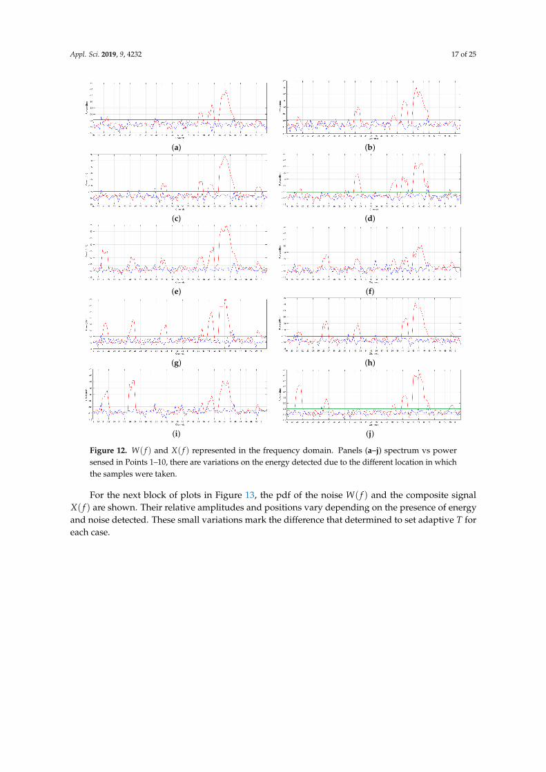
Using the same concept of the previously explained figure, Figures 12–14 show the spectrumdiagram, pdf of noise and composite signal, and ROC curve, respectively for ten different locations.In Figure 12a, for channel 21 and channels 39–45, we observe that the signal energy is above T. We alsoobserve that some noise peaks are also above T. This reading was taken in a location which is on theeastern end of the city. The subsequent readings were taken in a trajectory that approaches to thecentral part of the city. In Figure 12b, it is observed that signal energy is detected in channels 31 and32 in addition to the channels mentioned in Figure 12a. From Figure 12c, it appears that there areenergy peaks in channel 50 along with channels 31 and 32, but energy of channel 21 decreases to alevel below T. In Figure 12d, the energy of the detected channels maintains its values in relation tothe previous figure. In Figure 12e there are well-defined peaks of energy in channels 20–21, 26, 31–32,38 to 46, and 50. In Figure 12f, the profile is maintained, the general levels of energy decreases, but thesame channels are detected. For Panels (g), (h), (i), and (j), the detected energy does not present anysignificant variation and it is the usual energy profile of the channels detected in the central area of thecity. The channels detected are 20–21, 25–26, 31–32, 38 to 46, and 50.

Appl. Sci. 2019, 9, 4232 17 of 25

(a) (b)

(c) (d)

(e) (f)

(g) (h)

(i) (j)

Figure 12. W( f ) and X( f ) represented in the frequency domain. Panels (a–j) spectrum vs powersensed in Points 1–10, there are variations on the energy detected due to the different location in whichthe samples were taken.

For the next block of plots in Figure 13, the pdf of the noise W( f ) and the composite signalX( f ) are shown. Their relative amplitudes and positions vary depending on the presence of energyand noise detected. These small variations mark the difference that determined to set adaptive T foreach case.

Appl. Sci. 2019, 9, 4232 18 of 25

(a) (b) (c)

(d) (e) (f)

(g) (h) (i)

(j)

Figure 13. Each Panel contains a plot of the pdf of the signals sensed, from (a–j) pdf of the W( f ) andX( f ) taken in Points 1–10.

In Figure 14, the ROC curves from each of the ten locations are plotted. These curves representthe relation between Pf a and Pd in each case. The different values respond to the variations previouslyregistered in the sensed locations. These curves have enough information to reveal the behaviour ofthe spectrum.

Appl. Sci. 2019, 9, 4232 19 of 25

(a) (b) (c)

(d) (e) (f)

(g) (h) (i)

(j)

Figure 14. ROC that represents the relation of Pf a vs. Pd. Panels (a–j) ROC curves of the signal sensedin Points 1 to 10.

It is important to note that each reading provides valuable information to determine the state ofthe spectrum in that specific location at an instant of time ti. To obtain a global view of the proposedmethod and its applicability, it is necessary to compare all the obtained curves together to find a usablerelationship, if any. Figure 15a plots the ROC curves (Pf a vs Pd) of the ten analyzed locations. It isquite clear that each location has its own characteristics which differ from others. Figure 15b depictsthe same ROC curves shown in Figure 15a but focusing on a Pf a a range of 0% to 4%. Additionally,the dotted vertical lines represent the adaptive T in red, the T obtained with a M = 5 dBm in blue,M = 7 dBm in green, and M = 10 dBm in brown, respectively. The Y-coordinate value of the intersectionof a particular T and the ROC curve of a location represents Pd. For example in P3, for a Pf a of 3%,it corresponds to a 48.4% of Pd according to the vertical-axis scale of the ROC plot, and it means a96.8% of the Pdmax.

Appl. Sci. 2019, 9, 4232 20 of 25

(a) (b)

Figure 15. ROC curves obtained from P1–P10, in (a) are present all the curves, and in (b) are shown thesame plot but zooming in to observe the curves with a Pf a closer to the one defined by the adaptive Tof 3%.

To visualize the accuracy of the model that proposes an adaptive T, the curve of the Pf a vs Pd isobtained by calculating the average of 36,176 readings or 4,051,712 samples. By using Equations (5), (9),(15), and (16), the Pf amax is obtained and it corresponds to 4%. Figure 16 illustrates the average curve,the Pf amax, the adaptive T, and the values for T using a margin M of 5, 7, and 10 dB. Consideringthat Pf amax defines the Pdmax which becomes 99.999% of the signals that are possible to be detected,then the values of the Y-axis were re-calculated according to the new Pdmax scale. In gray color it canbe observed the recommended operation area, defined by the Pf amax, Pf amin, Pdmax, and Pdmin, and onthe left side of the plot, are the new re-calculated values for Pd.

Figure 16. Dotted lines are the Pf amax, Pf a calculated with the adaptive T, and T obtained by using aM of 5, 7, and 10 dB respectively. It is observed that the adaptive T proposed increases at lest 9.63% ofPd than the values used by other authors.

5.2. Discussing the Results

In this project, 33 UHF-TV channels (Channel 19 to channel 51), each having a bandwidth of6 MHz, were sensed. Channel 37 is assigned to radio astronomy and it is not used for TV broadcast,so that results were obtained for the remaining 32 TV channels. According to the information collectedand applying the proposed model, six channels were found to have enough energy above T and the PUpresence was confirmed. In Figure 17, the geographical points are plotted in which their occupationis represented.

Appl. Sci. 2019, 9, 4232 21 of 25

Figure 17. Location of the represented points.

5.3. Spectrum Sensed Results

In this sub-section, the obtained results are described. Figure 17 illustrates five locations, i.e.,Lab, (a), (b), (c), and (d), where data were sensed and represented. In Lab, we found the existenceof PU in 23 channels, so it shows 72% of TV spectrum used and 28% idle spectrum. The later maybe considered as potentially TVWS allowing DSA as SU. In Figure 18a, the results are plotted fordata taken in location (a), where we observe seventeen channels for which signal was detected (incyan), so that this is 53% of TV spectrum used, and 47% idle spectrum. Figure 18b corresponds tolocation (b) to the South of the city, where there are 16 channels for which signal was detected (incyan), representing 50% of used spectrum, and 50% of TVWS. In Figure 18c, which is the Middle-eastpart of the city, there are 15 channels for which signal was detected, which represents 50% of the usedspectrum, and 50% of TVWS. Finally, in Figure 18d, which shows the East limit of the city, there are13 channels for which signal was detected by the DAI (in cyan) so that this represents 40% of usedspectrum and 60% of TVWS.

(a) (b)

(c) (d)

Figure 18. Spectrum detected and analyzed with the proposed model: (a) Central south part of thecity, (b) South-east, (c) Middle East, and (d) Eastern limit of the city of Windsor. Note that as far of thecenter the sample is taken, less PUs are detected.

5.4. Variability of the Sensed Signals

The reason to take simultaneous samples of the noise W(p) and the composite signal X(p) at eachtime instant ti, responds to the variations experienced in the UHF-TV spectrum by the above-mentionedsignals. In Figure 19 we can observe the pdf of the average values for W(p) and X(p). To obtain thispdf, from trajectory T2, 1,166,928 samples were collected. The mean values of the signals were obtained,and a CI corresponding to 95% was calculated and plotted. Figure 19 also shows that the noise mean

Appl. Sci. 2019, 9, 4232 22 of 25

W(p) has a value of −108.9725 and can have a variation of 1.05 dB. The mean of the composite signalX(p) has a value of −103.9889 with a CI of 6.72 dB.

Around X(p), represented with a red dashed line, the mean of the composite signal values,could vary in 6.72 dB. Now, it means that sometimes the respective pdf of the noise and the compositesignal may be closer or separated from each other. This variation is confirmed by the plots representedin Figure 13. In order to avoid any error produced by the variation mentioned above, it is recommendedto obtain separate readings for signal and noise. This is more applicable when the M-SSS is used andthe samples are taken in different geographical locations every ti.

Figure 19. Confidence Interval (CI) of average values for W(p) and X(p), the variations are representedin dB.

5.5. Processing Time

According to Figure 3, the proposed model has six blocks in which the information of the UHF-TVspectrum is collected and processed. The action performed in each block, a brief explanation, and itsrespective average time is summarized in Table 4.

Table 4. Average time obtained in each block of the proposed model.

Block Action Performed Observations Time

1© Spectrum sensing Antenna/RFE collect samples W( f ), X( f ) 0.00 s2© Samples processing Two RFE save samples in DB 0.34 s3© Statistical calculations Matlab→ calculates W( f ), σW , X( f ), and σX 0.31 s4© Probability calculations With a selected Pf a, Matlab→ calculates M and T 0.24 s5© ED performing Matlab→ X( f ) is compared with T 0.27 s6© Results presentation Channel’s energy lower than T are marked as TVWS 0.29 s

Total 1.45 s

For blocks 1© and 2©, the time of the collected samples saved in the DB was obtained using the RFExplorer for Windows open software. For blocks 3© to 6©, the time was calculated in the Matlab scriptby using the start stopwatch timer command and running 500 times the mentioned script. To reducethe time in block 4©, we do not calculate the intersection point of two pdf curves W and X, in this case,we use the value of Pf a corresponding to 3%, and performing the operation explained in Equation (11),obtaining the value of T.

The total average time to find the TVWS in one reading is 1.45 s. To reduce it according tothe detection time suggested in the 802.22 standards [10], it is possible to use big data processingtechniques or use hardware with improved processing frequency, to achieve real-time detection.

Appl. Sci. 2019, 9, 4232 23 of 25

6. Conclusions

A probabilistic model for identifying TVWS has been proposed. The model was based on theprobabilistic analysis performed on collected spectrum information in the city of Windsor, Canada.To collect the spectrum information over a wide geographical area, a vehicle-mounted M-SSS wasdesigned and implemented. It uses light weight components, consumes low power, and is easyto handle.

A noteworthy feature of the M-SSS is that it uses two RFE devices connected in parallel for sensingthe composite signal X( f ) and noise signal W( f ) simultaneously. This individual sensing enablesour model to yield better accuracy. Based on this simultaneously sensed data, the model uses twostatistical parameters, i.e., the false alarm probability and the detection probability to calculate anadaptive threshold.

The false alarm probability and the detection probability values are calculated based on theconsideration that both the noise signal and the composite signal follow Normal distribution. In reality,the noise signal truly follows a Normal distribution as verified by the Kolmogorov–Smirnov testperformed in our work, but the composite signal actually is a multi modal signal. In order to reducecomputational complexity related to probabilistic analysis, the composite signal has also been assumedto follow the Normal distribution. We consider this assumption is acceptable, and it does not hamperthe detection accuracy of our model. This is because the fundamental calculations involved in findingthe false alarm probability is based only on the noise signal, which as mentioned before, indeed followsa Normal distribution. The optimal false alarm probability is used as an input in the receiver operatingcharacteristic curve function, and the optimal detection probability is obtained.

In terms of performance, the proposed model demonstrates about 9.6% higher detectionprobability (Pd) compared to other methods found in literature. From our collected data, we observedthat in the central area of the city, about 28% of the sensed spectrum are TVWS and as we move to theouter edges of the city, up to 60% of the TV channels sensed were found to be TVWS.

This observation clearly suggests that there lies a significant number of unused TV channels whichcan be used for different opportunistic services through the implementation of cognitive radio-enableddynamic spectrum access. Finally, it can be concluded that the proposed mobile spectrum sensingstation along with the proposed probabilistic model for sensing the UHF-TV spectrum may be used inany other location.

Author Contributions: D.C.-D.-W. collected and organized the data presented in this paper and analyzed theinformation. D.C.-D.-W., S.A. and J.L.R.-A. wrote and reviewed the manuscript, analyzing the most relevant data.F.A. and K.T. reviewed and discussed the manuscript.

Acknowledgments: This work was supported by the Secretaría de Educación Superior, Ciencia, Tecnología eInnovación of Ecuador and the University of Windsor. Authors thank to the WiCIP Lab for providing all theequipment necessary to collect the information which is analyzed and discussed in this manuscript.

Conflicts of Interest: The authors declare no conflict of interest.

References

1. Liang, Y.C.; Chen, K.C.; Li, G.Y.; Mahonen, P. Cognitive radio networking and communications: An overview.IEEE Trans. Veh. Technol. 2011, 60, 3386–3407. [CrossRef]

2. Datla, D.; Wyglinski, A.M.; Minden, G.J. A spectrum surveying framework for dynamic spectrum accessnetworks. IEEE Trans. Veh. Technol. 2009, 58, 4158–4168. [CrossRef]

3. Liu, Y.; Ding, Z.; Elkashlan, M.; Yuan, J. Nonorthogonal multiple access in large-scale underlay cognitiveradio networks. IEEE Trans. Veh. Technol. 2016, 65, 10152–10157. [CrossRef]

4. Brown, T.X.; Pietrosemoli, E.; Zennaro, M.; Bagula, A.; Mauwa, H.; Nleya, S.M. A survey of TV white spacemeasurements. In International Conference on e-Infrastructure and e-Services for Developing Countries; Springer:Berlin/Heidelberg, Germany, 2014; pp. 164–172.

5. Shellhammer, S.J. Spectrum Sensing in IEEE 802.22. In Proceedings of the IAPR Workshop on CognitiveInformation Processing, Santorini, Greece, 9–10 June 2008; pp. 9–10.

Appl. Sci. 2019, 9, 4232 24 of 25

6. Mitola, J.; Maguire, G.Q. Cognitive radio: Making software radios more personal. IEEE Pers. Commun. 1999,6, 13–18. [CrossRef]

7. Haykin, S. Cognitive radio: Brain-empowered wireless communications. IEEE J. Sel. Areas Commun. 2005,23, 201–220. [CrossRef]

8. Cordeiro, C.; Challapali, K.; Birru, D.; Shankar, S. IEEE 802.22: An introduction to the first wireless standardbased on cognitive radios. J. Commun. 2006, 1, 38–47.

9. Rusch, L.A. Indoor wireless communications: Capacity and coexistence on the unlicensed bands.Int. Technol. J. 2001, 3, 2001.

10. IEEE. IEEE 802.22 Working Group on Wireless Regional Area Networks. Available online: http://www.ieee802.org/22/ (accessed on 31 March 2019).

11. Zeng, Y.; Liang, Y.C. Eigenvalue-based spectrum sensing algorithms for cognitive radio. IEEE Trans. Commun.2009, 57, 1784–1793. [CrossRef]

12. Pietrosemoli, E.; Zennaro, M. TV White Spaces—A Pragmatic Approach. In Proceedings of the SixthInternational Conference on Information and Communication Technologies and Development, Cape Town,South Africa, 7–10 December 2013.

13. Chen, Y.; Oh, H.S. A survey of measurement-based spectrum occupancy modeling for cognitive radios.IEEE Commun. Surv. Tutor. 2016, 18, 848–859. [CrossRef]

14. Manesh, M.R.; Subramaniam, S.; Reyes, H.; Kaabouch, N. Real-time spectrum occupancy monitoring usinga probabilistic model. Comput. Netw. 2017, 124, 87–96. [CrossRef]

15. Akyildiz, I.F.; Lee, W.Y.; Vuran, M.C.; Mohanty, S. NeXt generation/dynamic spectrum access/cognitiveradio wireless networks: A survey. Comput. Netw. 2006, 50, 2127–2159. [CrossRef]

16. Federal Communications Commission (FCC). Docket No 03-222 Notice of Proposed Rule Making andOrder. Available online: https://web.cs.ucdavis.edu/~liu/289I/Material/FCC-03-322A1.pdf (accessed on26 September 2019).

17. Jing, X.; Raychaudhuri, D. Spectrum co-existence of IEEE 802.11 b and 802.16 a networks using the CSCCetiquette protocol. In Proceedings of the First IEEE International Symposium on New Frontiers in SpectrumAccess Networks, Baltimore MD, USA, 8–11 November 2005; pp. 243–250.

18. Akhtar, F.; Rehmani, M.H.; Reisslein, M. White space: Definitional perspectives and their role in exploitingspectrum opportunities. Telecommun. Policy 2016, 40, 319–331. [CrossRef]

19. International Telecommunications Union (ITU). Frequency Bands allocated to Terrestrial BroadcastingServices. Available online: https://www.itu.int/en/ITU-R/terrestrial/broadcast/Pages/Bands.aspx(accessed on 26 September 2019).

20. Corral-De-Witt, D.; Younan, A.; Fatima, A.; Matamoros, J.; Awin, F.A.; Tepe, K.; Abdel-Raheem, E. Sensing tvspectrum using software defined radio hardware. In Proceedings of the 2017 IEEE 30th Canadian Conferenceon Electrical and Computer Engineering (CCECE), Windsor, ON, Canada, 30 April–3 May 2017; pp. 1–4.

21. Awin, F.; Younan, A.; Corral-De-Witt, D.; Tepe, K.; Abdel-Raheem, E. Real-Time Multi-Channel TVWSSensing Prototype Using Software Defined Radio. In Proceedings of the 2018 IEEE International Symposiumon Signal Processing and Information Technology (ISSPIT), Louisville, KY, USA, 6–8 December 2018;pp. 212–217.

22. RF Explorer. RF Explorer Spectrum Analyzer. Available online: http://j3.rf-explorer.com/40-rfe/article/48-introducing-rf-explorer (accessed on 29 March 2019).

23. Tektronix. MDO 4000 Series Manual. Available online: https://www.tek.com/oscilloscopes/mdo4000-manual/mdo4000-series-0 (accessed on 29 March 2019).

24. Lekomtcev, D.; Maršálek, R. Comparison of 802.11 af and 802.22 standards–physical layer and cognitivefunctionality. Elektro Revue 2012, 3, 12–18.

25. Harrold, T.; Cepeda, R.; Beach, M. Long-term measurements of spectrum occupancy characteristics.In Proceedings of the 2011 IEEE International Symposium on Dynamic Spectrum Access Networks (DySPAN),Aachen, Germany, 3–6 May 2011; pp. 83–89.

26. Valenta, V.; Maršálek, R.; Baudoin, G.; Villegas, M.; Suarez, M.; Robert, F. Survey on spectrum utilization inEurope: Measurements, analyses and observations. In Proceedings of the 2010 Fifth International Conferenceon Cognitive Radio Oriented Wireless Networks and Communications, Cannes, France, 16–18 June 2010;pp. 1–5.

Appl. Sci. 2019, 9, 4232 25 of 25

27. Qaraqe, K.A.; Celebi, H.; Gorcin, A.; El-Saigh, A.; Arslan, H.; Alouini, M.S. Empirical results for widebandmultidimensional spectrum usage. In Proceedings of the 2009 IEEE 20th International Symposium onPersonal, Indoor and Mobile Radio Communications, Tokyo, Japan, 13–16 September 2009; pp. 1262–1266.

28. Awin, F.; Abdel-Raheem, E.; Tepe, K. Blind spectrum sensing approaches for interweaved cognitive radiosystem: A tutorial and short course. IEEE Commun. Surv. Tutor. 2018, 21, 238–259. [CrossRef]

29. Awin, F.A.; Alginahi, Y.M.; Abdel-Raheem, E.; Tepe, K. Technical Issues on Cognitive Radio-Based Internetof Things Systems: A Survey. IEEE Access 2019, 7, 97887–97908. [CrossRef]

30. Chambers, J.M. Graphical Methods for Data Analysis: 0; Chapman and Hall/CRC: Boca Raton, FL, USA, 2017.31. Massey, F.J., Jr. The Kolmogorov–Smirnov test for goodness of fit. J. Am. Stat. Assoc. 1951, 46, 68–78.

[CrossRef]32. Z Table. Z Score Table. Available online: http://www.z-table.com/ (accessed on 18 April 2019).33. Brown, C.D.; Davis, H.T. Receiver operating characteristics curves and related decision measures: A tutorial.

Chemom. Intell. Lab. Syst. 2006, 80, 24–38. [CrossRef]34. International Telecommunications Union ITU. Handbook Spectrum Monitoring, Chapter 3.

Available online: https://extranet.itu.int/brdocsearch/R-HDB/R-HDB-23/R-HDB-23-2002/R-HDB-23-2002-OAS-PDF-E.pdf (accessed on 29 March 2019).

c© 2019 by the authors. Licensee MDPI, Basel, Switzerland. This article is an open accessarticle distributed under the terms and conditions of the Creative Commons Attribution(CC BY) license (http://creativecommons.org/licenses/by/4.0/).