An accurate and linear-scaling method for calculating charge-transfer excitationenergies and diabatic couplingsMichele Pavanello, Troy Van Voorhis, Lucas Visscher, and Johannes Neugebauer

Citation: The Journal of Chemical Physics 138, 054101 (2013); doi: 10.1063/1.4789418 View online: http://dx.doi.org/10.1063/1.4789418 View Table of Contents: http://scitation.aip.org/content/aip/journal/jcp/138/5?ver=pdfcov Published by the AIP Publishing Articles you may be interested in Assessment of charge-transfer excitations with time-dependent, range-separated density functional theory basedon long-range MP2 and multiconfigurational self-consistent field wave functions J. Chem. Phys. 139, 184308 (2013); 10.1063/1.4826533 Charge transfer excited state energies by perturbative delta self consistent field method J. Chem. Phys. 137, 084316 (2012); 10.1063/1.4739269 Accurate potential energy surface and quantum reaction rate calculations for the H + C H 4 H 2 + C H 3 reaction J. Chem. Phys. 124, 164307 (2006); 10.1063/1.2189223 Vibronic coupling and double excitations in linear response time-dependent density functional calculations:Dipole-allowed states of N 2 J. Chem. Phys. 121, 6155 (2004); 10.1063/1.1785775 Charge-transfer correction for improved time-dependent local density approximation excited-state potentialenergy curves: Analysis within the two-level model with illustration for H 2 and LiH J. Chem. Phys. 113, 7062 (2000); 10.1063/1.1313558

This article is copyrighted as indicated in the article. Reuse of AIP content is subject to the terms at: http://scitation.aip.org/termsconditions. Downloaded to IP:

95.130.38.103 On: Fri, 11 Apr 2014 16:48:11

THE JOURNAL OF CHEMICAL PHYSICS 138, 054101 (2013)

An accurate and linear-scaling method for calculating charge-transferexcitation energies and diabatic couplings

Michele Pavanello,1,a) Troy Van Voorhis,2 Lucas Visscher,3 and Johannes Neugebauer4,b)

1Department of Chemistry, Rutgers University, Newark, New Jersey 07102-1811, USA2Department of Chemistry, Massachusetts Institute of Technology, Cambridge,Massachusetts 02139-4307, USA3Amsterdam Center for Multiscale Modeling, VU University, De Boelelaan 1083,1081 HV Amsterdam, The Netherlands4Theoretische Organische Chemie, Organisch-Chemisches Institut der WestfälischenWilhelms-Universität Münster, Corrensstraße 40, 48149 Münster, Germany

(Received 7 November 2012; accepted 11 January 2013; published online 1 February 2013)

Quantum–mechanical methods that are both computationally fast and accurate are not yet avail-able for electronic excitations having charge transfer character. In this work, we present a signif-icant step forward towards this goal for those charge transfer excitations that take place betweennon-covalently bound molecules. In particular, we present a method that scales linearly with thenumber of non-covalently bound molecules in the system and is based on a two-pronged approach:The molecular electronic structure of broken-symmetry charge-localized states is obtained with thefrozen density embedding formulation of subsystem density-functional theory; subsequently, in apost-SCF calculation, the full-electron Hamiltonian and overlap matrix elements among the charge-localized states are evaluated with an algorithm which takes full advantage of the subsystem DFTdensity partitioning technique. The method is benchmarked against coupled-cluster calculations andachieves chemical accuracy for the systems considered for intermolecular separations ranging fromhydrogen-bond distances to tens of Ångstroms. Numerical examples are provided for molecular clus-ters comprised of up to 56 non-covalently bound molecules. © 2013 American Institute of Physics.[http://dx.doi.org/10.1063/1.4789418]

I. INTRODUCTION

Charge transfer (CT) reactions are ubiquitous in allbranches of chemistry, and huge efforts have been spent inthe past to analyze these processes in terms of theoreticalmodels.1–3 They can be categorized into processes in whicha charge separation in a donor–acceptor system takes place,

D + A → D+ + A−, (1)

and processes where the charge has been externally created(either by injecting or removing an electron),

D− + A → D + A−, (2)

D+ + A → D + A+, (3)

where we define D as the donor and A as the acceptor. Forthe reactions in (1) and (2), donor and acceptor are defined interms of donating and receiving electrons, while in (3) thedefinitions are in terms of the location of the excess posi-tive charge. The three kinds of CT reactions in (1)–(3) areinvolved in a plethora of important processes. For example,(1) may resemble a charge splitting event either at a semicon-ductor interface, between an organic dye and a semiconductor,or the charge separation event in the reaction centers of photo-synthetic systems. Generally, all the charge separation events

a)E-mail: m.pavanello@rutgers.edu.b)E-mail: j.neugebauer@uni-muenster.de.

can be thought of in terms of a two-state model comprisedof a neutral state and a charge separated state. Throughoutthis work, we call the reactions involving only the motion ofan excess of charge, as in (2) and (3), migration CT (MCT,hereafter) reactions. MCT reactions are the simplest type ofreactions involving CT states, and take place in many fun-damental processes related to charge mobility, transport, andenzyme functionality. In these processes, the charge separa-tion event has happened in the past, and the problem shifts tothe prediction of the kinetics of the excess charge, may thatbe across a polymer4–6 (organic electronics), a protein (en-zyme functionality7, 8 and photosynthesis9, 10), or DNA11–13

(oxidative damage).Very often, the ground and MCT states are close in en-

ergy and one easily finds the first MCT state as being the firstexcited state of the system. This is an important advantage intheoretical studies of this type of states as opposed to othertypes of excited states for which the excited state search canbe a daunting task. Another important quality of MCT statesis the simple physical depiction of ground and excited states:the former has an excess charge on the, say, “left,” and thelatter features an excess charge on the “right.” Obviously, thissimple depiction becomes more complicated as soon as thesystem under study contains more than two chemical moi-eties capable of accepting/donating an excess charge. Theseunique qualities make MCT states a perfect testbed for newcomputational methods aiming at the accurate prediction ofgenerally all kinds of CT excitations.

0021-9606/2013/138(5)/054101/12/$30.00 © 2013 American Institute of Physics138, 054101-1

This article is copyrighted as indicated in the article. Reuse of AIP content is subject to the terms at: http://scitation.aip.org/termsconditions. Downloaded to IP:

95.130.38.103 On: Fri, 11 Apr 2014 16:48:11

054101-2 Pavanello et al. J. Chem. Phys. 138, 054101 (2013)

There are two fundamentally different schemes for cal-culating CT excitations. The first one involves the construc-tion of Hamiltonian and overlap matrices in a basis of charge-localized broken-symmetry states. This basis set is oftencalled a diabatic basis set, and the basis functions termed di-abatic states. The chosen broken-symmetry states in the setshould resemble the true ground and the CT excited statesof the system. Depending on the size of the basis set (orequivalently the number of broken-symmetry states includedin the calculation) the simultaneous diagonalization of over-lap and Hamiltonian matrices (i.e., solving the generalizedeigenvalue problem) yields the sought ground and CT excitedstates. The latter diagonalization step is similar to the diag-onalization step in the configuration interaction (CI) methodcarried out with valence bond configuration state functions.Even though this is a general method, it is particularly suitedfor the calculation of CT excited states. This is because con-trary to valence excitations, the broken-symmetry basis func-tions assume a simple charge-localized character and rela-tively uncomplicated computational criteria can be devisedfor their generation.14–20 This is the method that we use inthis work and is described in detail in Sec. II for a basisset comprised of two broken-symmetry states. Contrary tothe first scheme mentioned above, the alternative is not tai-lored specifically to CT excitations and it involves obtainingdirectly the adiabatic ground and excited states of the sys-tem. As such it is more general than the first scheme and ismost often adopted in the literature. Due to the high computa-tional throughput of modern computers, calculations based onthe latter scheme are now commonplace. A plethora of quan-tum chemistry methods are devoted to the prediction of ex-cited states’ energies, transition moments, densities, and wavefunctions. Despite this, CT excited states have always beenmore challenging than others, because for this kind of excita-tions the electron density changes dramatically compared tothe ground state one. Density-functional theory (DFT), andspecifically its time-dependent extension (TD-DFT) throughthe linear-response formalism for the calculation of electronicexcitations and transition moments21 has struggled to cor-rectly deal with CT excitations when employing approxi-mate density functionals.22 Pragmatic corrections exist, suchas the one originally developed by Gritzenko et al.,23, 24 orthe one involving the Peach factor.25 Range separated26–28

density functionals have also offered an effective solutionto the problem by enforcing the correct long-range behaviorat the price of including yet another parameter to the den-sity functional (the range separation parameter, often denotedby γ ). Methodologies to obtain γ parameters which satisfycertain system-dependent and process-dependent conditionshave been proposed.29, 30 Novel computational approaches toobtain charge-transfer excited states within a DFT formalismare being explored. Specifically, a variational formulation ofTD-DFT31 has shown to alleviate or to completely cure theCT excitation failures of linear-response TD-DFT when thefourth-order relaxed constrained-variational TD-DFT methodis employed, however, at the expense of higher computationalcomplexity than standard linear-response TD-DFT.

Wave function based methods also have encountered dif-ficulties when approaching CT excitations. The low end of

wave function methods, configuration interaction with singles(CIS), and time-dependent Hartree–Fock (TD-HF) are knownto grossly overestimate CT excitation energies.32–36 More bal-anced methods, such as multi-configuration self-consistentfield (MCSCF), multi-reference CI (MR-CI), or perturbativecorrections to CIS, such as CIS(D), as well as ADC(2)37 areable to deliver good CT excitation energies32, 38 and are of-ten taken as benchmark.39 MCSCF, however, is known tofail near avoided crossings (a feature always present in sys-tems featuring MCT excitations) unless state averaging isemployed.40 The equation-of-motion coupled cluster (EOM-CC) theory40, 41 is also known to fail in reproducing CT exci-tations with a similar accuracy than ionization potentials andelectron affinities42, 43 due to its non size-extensivity stem-ming from the non-exponential form of the EOM-CC ansatzfor the excited states. Linear-response CC, and specifically anapproximation to it including only single and double excita-tions known as CC2 has been very successful in predictingCT excitations.44–47 A particularly powerful implementationof CC2 utilizing the resolution of the identity (RI-CC2)48 isroutinely applied to systems with up to 100 atoms. It is nowunderstood that to obtain an accurate description of CT exci-tations the employed method must describe the dynamic cor-relation of the CT excited states similarly to the one of theground state.49 In addition, the computational costs associatedwith all the wave function methods mentioned above (with theexception of TD-HF and CIS) are prohibitive for most sys-tems in condensed-phase and biosystems of interest.

In Sec. II, we will describe in detail how ground andCT excited state energies and wave functions can be obtainedstarting from a basis set comprised of two broken-symmetrystates. In Sec. III we will introduce the frozen density em-bedding formulation of subsystem DFT (a linear-scaling,full-electron electronic structure method) which we use todetermine the electronic structure of the broken-symmetry,charge-localized states. Then in Sec. IV we will present thetheory behind the calculation of the full-electron Hamiltonianand overlap matrix elements among the broken-symmetrystates (generated with subsystem DFT) which we have imple-mented in the Amsterdam density functional (ADF) computersoftware.50, 51 Section V is devoted to benchmarking of themethod for three selected cases of MCT, e.g., hole transfer inwater and ethylene dimers at several inter-monomer separa-tions and geometries, and DNA nucleobase dimers. SectionVI features two pilot calculations of the hole transfer in waterand ethylene clusters containing up to 56 and 20 molecules,respectively.

II. EXCITATION ENERGIES FROM A MODEL OF TWOBROKEN-SYMMETRY STATES

Consider a system comprised of a charge donor and acharge acceptor moiety in the absence of low-lying interme-diate bridge states (DA system hereafter). Such a system canbe well characterized by a two-state formalism. That is, it isenough to consider either the adiabatic ground and first ex-cited state or a set of two broken-symmetry charge-localizedstates to capture most of the underlying physics. There is alarge literature15, 16, 52–54 supporting the idea that the states

This article is copyrighted as indicated in the article. Reuse of AIP content is subject to the terms at: http://scitation.aip.org/termsconditions. Downloaded to IP:

95.130.38.103 On: Fri, 11 Apr 2014 16:48:11

054101-3 Pavanello et al. J. Chem. Phys. 138, 054101 (2013)

with localized excess charges, i.e., one where the charge islocalized on the donor and, conversely, one where the chargeis localized on the acceptor, are an appropriate basis for mod-eling the process of charge migration between donor andacceptor.

A state with localized charges generally is not the groundstate of the system Hamiltonian. Therefore, in the basisof charge-localized states, the Hamiltonian matrix is non-diagonal. In addition, as these states are of broken-symmetrycharacter, they are generally non-orthogonal to each other.Throughout this work, we will refer to the full-electron wavefunctions of the two charge-localized states as �1 and �2. ForDA systems, the Hamiltonian (H) and overlap matrices (S) inthis basis are of dimension 2 × 2, namely,

H =(

H11 H12

H21 H22

)(4)

and

S =(

1 S12

S12 1

). (5)

The definitions in Eqs. (4) and (5) allow us to obtain the CTexcitation energy as the energy difference of the orthonormaladiabatic states, which can be obtained by solving the gener-alized eigenvalue problem,∣∣∣∣∣ H11 − E H12 − ES12

H21 − ES12 H22 − E

∣∣∣∣∣ = 0. (6)

The above equation yields two energy eigenvalues (say E1 andE2) and their difference (�E) is the sought CT excitation. Ina closed form, we obtain52, 53, 55

�E =√

(H11 − H22)2

1 − S212

+ 4V 212, (7)

where V12 = 11−S2

12[H12 − S12

H11+H222 ].

The problem is then shifted to calculating four matrix el-ements, i.e., the two diagonal Hamiltonian elements (H11 andH22, e.g., the total energies of the charge-localized states ordiabatic energies), the H12 off-diagonal matrix element, andthe S12 overlap element. The V12 element introduced above iscommonly referred to as electronic coupling.

Several methods and algorithms have been proposedto generate ad hoc charge-localized states and to calculatethe above matrix elements both for purely wave functionmethods16, 18, 19, 56–58 as well as DFT methods.14, 15, 17, 53, 59–62

Regular wave function and DFT methods tend to scale non-linearly with the system size. Therefore, important systemsof biological interest, large organics and hybrid organic–inorganic systems (such as dye-sensitized solar cells) arelargely out of reach of these methods unless truncated modelsystems or substantial approximations are introduced at theelectronic structure theory level.

In this work, we build upon ideas presented in aprevious paper62 and we construct the broken-symmetrycharge-localized states using a linear-scaling technique calledfrozen density embedding.63 The construction of the charge-localized, diabatic states is a prerequisite in this formalism for

the calculation of the CT excitation energies. A brief descrip-tion of this technique follows this section.

III. THE FROZEN DENSITY EMBEDDINGFORMULATION OF SUBSYSTEM DFT

Subsystem DFT is a successful alternative to regularKohn–Sham (KS) DFT methods due to its ability to over-come the computational difficulties arising when tacklinglarge molecular systems.64 One particular variant of subsys-tem DFT is the Frozen Density Embedding (FDE) approachdeveloped by Wesolowski and Warshel.63 FDE splits a sys-tem into interacting subsystems and yields subsystem elec-tron densities separately. Hence, it defines the total electrondensity, ρ(r), as a sum of subsystem densities,63

ρ(r) =# of subsystems∑

I

ρI (r), (8)

where the sum runs over all subsystems. The subsystem den-sities are found by solving subsystem-specific KS equations,known as KS equations with constrained electron density orKSCED.65 In these equations, the KS potential vKS(r) is aug-mented by an embedding potential vemb(r) which includes theelectrostatic interactions taking place between electrons andnuclei of the subsystems as well as a potential term derivingfrom the non-additive kinetic energy (T nadd

s ) and non-additiveexchange-correlation (Enadd

xc ) functional derivatives. We referto Refs. 63, 65, and 66 for more details on the FDE theoreti-cal framework, however, for sake of clarity we report here thespin KSCED equations which lead to the subsystem orbitals[−∇2

2+ vIσ

KS(r) + vIσemb(r)

]φσ

(i)I (r) = εσ(i)I φ

σ(i)I (r), (9)

where φσ(i)I

are the molecular orbitals of subsystem I and ofspin σ .

The FDE scheme greatly reduces the computational costcompared to KS-DFT, as there is no need to calculate or-bitals for the total (“super”) system, and the total computa-tional complexity is then linear over the number of subsys-tems composing the total supersystem. However, the reducedcost in FDE compared to KS-DFT is achieved at the expenseof approximating the non-additive functionals with semilocaldensity-functional approximants. This approximation, for thekinetic energy especially, is the single source of certain short-comings of FDE, for example, when applied to covalentlybound subsystems.67

IV. CHARGE TRANSFER EXCITATIONS WITH FDE

Recently, two of the present authors have shown inRef. 62 that FDE can be successfully used to calculate mi-gration CT couplings and excitation energies. In this work,we present a different algorithm for obtaining the elementsof the full-electron Hamiltonian and overlap matrices definedin Eqs. (4) and (5) which has significant advantages over theprevious method. Specifically, the new formalism can be ap-plied to symmetric systems (out of reach before due to asingularity in the working equations20, 62) and, as it will be

This article is copyrighted as indicated in the article. Reuse of AIP content is subject to the terms at: http://scitation.aip.org/termsconditions. Downloaded to IP:

95.130.38.103 On: Fri, 11 Apr 2014 16:48:11

054101-4 Pavanello et al. J. Chem. Phys. 138, 054101 (2013)

clear in Sec. V, yields very accurate excitation energies withmainstream GGA-type functionals, while before it was nec-essary to include HF non-local exchange to the functional tocounteract the self-interaction error. In addition, two newalgorithms have been implemented here. We call themsubsystem-joint transition density (JTD) and subsystem-disjoint transition density (DTD) formalisms. While the for-mer is computationally straightforward, it formally does notscale linearly with the number of subsystems. Instead, the lat-ter scales linearly with the number of subsystems and, thus, itis theoretically consistent with the FDE formalism.

A. Approximate couplings and total energiesin subsystem DFT

Suppose we have two broken-symmetry Slater determi-nants describing two charge-localized states �1 and �2. Thewave functions in terms of the two set of molecular orbitalstake the form:

�i = A[φ

(i)1 φ

(i)2 . . . φ

(i)N

], (10)

where the antisymmetrizer A also contains appropriate nor-malization constants. Generally, the two sets of molecularorbitals {φ(1)

k } and {φ(2)k } may not be orthonormal to each

other and within the sets. This usually happens for broken-symmetry HF and KS-DFT solutions as well as for KS-determinants derived from constrained DFT14 and subsystemDFT calculations.62 We define the transition orbital overlapmatrix as follows:

(S(12))kl = ⟨φ

(1)k

∣∣φ(2)l

⟩. (11)

In what follows, we only consider the case of a subsystemDFT calculation, i.e., we only deal with Slater determinants ofthe system constructed form subsystem molecular orbitals asdone in a previous work.62 To avoid redundance with the the-ory of Ref. 62, let us briefly state that, similarly to the valencebond theory,57 the subsystem DFT version of the Slater deter-minant in Eq. (10) features products of occupied subsystemorbitals regardless of the fact that the orbitals between sub-systems might not be orthogonal to each other. In the case ofa two-subsystem partitioning, the S(12) transition orbital over-lap matrix can be formally written as

S(12) =⎛⎝ S(12)

I S(12)I,II

S(12)II,I S(12)

II

⎞⎠ , (12)

where S(12)I and S(12)

II are transition orbital overlap matricescalculated with the orbitals belonging to subsystem I or II,respectively (subsystem transition orbital overlap matrices,hereafter), while S(12)

I,II and S(12)II,I include the overlaps of the

orbitals belonging to subsystem I with the ones belonging tosubsystem II. Let us clarify that there are two sources of non-orthogonality in this formalism. The first one stems from theoverlap between the full-electron charge-localized states, i.e.,Eq. (5), and the second one arises at the (subsystem) molec-ular orbital level in Eqs. (10) and (11). The orbital overlapmatrix is generally non-diagonal, also when it is computed

from orbitals belonging to a single state, namely,

(S(ii))kl = ⟨φ

(i)k

∣∣φ(i)l

⟩. (13)

It can be seen that the above matrix also is non-diagonal asthe orbitals {φ(i)

k }k=1,N are borrowed from an FDE calculationwhich does not impose orthogonality to orbitals belonging todifferent subsystems.63, 68

Going back to the elements of the S(12)I,II and S(12)

II,I subma-trices, it is clear that they are small in magnitude comparedto the subsystem transition overlap matrices provided that thesubsystems are not covalently bound to each other. The ma-trix form in Eq. (12) partially loses its block form in the caseof electronic transitions that change the number of electronsin the subsystems, such as the ones considered in this work.Specifically, if the CT transition involves one electron, thenthe transition overlap matrix will have one column (row) withsizable non-zero elements across the subsystems involved inthe CT event.

In this work, we use the following formulas for the cal-culation of the Hamiltonian coupling between the two charge-localized states:14, 69

H12 = 〈�1|H |�2〉 = E[ρ(12)(r)]S12, (14)

where S12 = det(S(12)), and

ρ(12)(r) =∑kl

φ(1)k (r)(S(12))−1

kl φ(2)l (r) (15)

is a scaled transition density derived from the orbitals of thetwo states, and the functional E is an appropriate density func-tional. The transition density in Eq. (15) is obtained from theintegration of the one-particle Dirac delta function, namely,70

〈�1|Nδ(r1 − r)|�2〉 = N

∫dr1 · · · drN�1(r1 · · · rN )

× δ(r1 − r)�2(r1 · · · rN )

=∑kl

D(12)(k|l)φ(1)k (r)φ(2)

l (r)

= det(S(12))∑kl

φ(1)k (r)(S(12))−1

kl φ(2)l (r),

(16)

where D(12)(k|l) is the signed minor (or cofactor) of the tran-sition orbital overlap matrix of Eq. (11). Then Eq. (15) is ob-tained by simply dividing Eq. (16) by det(S(12)), so that thescaled transition density integrates to the total number of elec-trons (N) rather than to N det(S(12)).

Scaling the transition density is a matter of algebraic con-venience. Equation (14) is particularly simple in terms of ascaled transition density, and is rigorous if the wave func-tions are single Slater determinants and the Hamiltonian isthe molecular electronic Hamiltonian69, 71–73 (i.e., as in the HFmethod). In our work, we consider two charge-localized statesper calculation. These are generally non-orthogonal. How-ever, for some systems, it is possible that the two states couldaccidentally be orthogonal. In this scenario, the scaled transi-tion density is recovered by employing the Penrose inverseof the transition overlap matrix in Eq. (15). The matrix is

This article is copyrighted as indicated in the article. Reuse of AIP content is subject to the terms at: http://scitation.aip.org/termsconditions. Downloaded to IP:

95.130.38.103 On: Fri, 11 Apr 2014 16:48:11

054101-5 Pavanello et al. J. Chem. Phys. 138, 054101 (2013)

inverted in the N − x dimensional subspace (usually x = 1)where it is not singular.

It is important to point out that the coupling formula inEq. (14) was derived assuming that �1/2 are broken-symmetryHF wave functions. Even though the HF and KS wave func-tions are both single Slater determinants, the formula is notformally transferable from the HF method to a DFT method(as we do in this work). Applying Eq. (14) in the context ofDFT is an approximation. It can be shown that in the con-text of linear-response TD-DFT Eqs. (14) and (15) are equiv-alent to the Tamm-Dancoff approximation to TD-DFT. In ad-dition, let us clarify that formally the HF exchange and HFand KS kinetic energy terms are computed with the transi-tion density matrix, and thus the density in Eq. (15) should bereplaced by a quantity that depends on one electronic coordi-nate r as well as another electronic coordinate, r′, namely,ρ(12)(r, r′) = ∑

kl φ(1)k (r)(S(12))−1

kl φ(2)l (r′). However, for sake

of clarity, here we will limit ourselves to reporting the (transi-tion) density without introducing the density matrix notation.As an example of how we apply Eq. (14) in practical calcu-lations, consider a calculation in which we employ the LDAexchange density functional, then the exchange contributionto the off-diagonal Hamiltonian matrix element becomes

Ex[ρ(12)(r)]S12 = −S123

4

(3

π

) 13∫

(ρ(12)(r))43 dr. (17)

The diagonal elements of the Hamiltonian are computedin a similar fashion as the off-diagonal ones, namely,

Hii = 〈�i |H |�i〉 = E[ρ(i)(r)], (18)

where

ρ(i)(r) =∑kl

φ(i)k (r)(S(ii))−1

kl φ(i)l (r). (19)

Note that the overlap element has disappeared in Eq. (18).While this is a trivial consequence of the normalization con-dition on the Slater determinant in a regular KS-DFT cal-culation, the KS Slater determinant of the supersystem builtwith subsystem orbitals is not normalized. However, the cor-responding FDE density theoretically is the correctly normal-ized correlated density of the full system, integrating to thetotal number of electrons.62 This is an important point as thenumber of electrons in a calculation is set by the trace ofthe (transition or diagonal) orbital overlap matrix, while thenorm of a Slater determinant depends upon the determinantof the corresponding orbital overlap matrix.

To summarize, the approximations we employ are equiv-alent to (1) replacing the HF Slater determinants needed todefine the charge-localized states �1/2 with Slater determi-nants made up of subsystem KS molecular orbitals, and (2)replacing the HF expression of E[ρ(12)(r)] by an approximatedensity functional.

Approximation (1) is often invoked in DFT calculationsof electronic couplings,14, 15, 53, 59, 62 while (2) was used beforeby Kaduk et al.,14 and it is introduced here for the first time inthe context of subsystem DFT. Contrary to the density, thescaled transition density introduced in Eq. (15) might fea-ture regions of space where it carries a negative sign. Gener-

ally, exchange-correlation and kinetic-energy functionals mayfeature arbitrary fractional powers of the density that wouldrender the exchange-correlation energy complex. By work-ing with a scaled transition density that is quasi-positive al-most everywhere in space (see below), the simplest pragmaticworkaround is to set the scaled transition density to zero ev-erywhere in space where it actually has negative values. Whilethis may seem to be a somewhat drastic approximation, wenote that in practice only a small part of the scaled transi-tion density needs to be changed, and the very good resultsobserved in our test cases below empirically justify this pro-cedure (see Sec. V). In all the cases considered here, the ne-glect of the negative parts of the scaled transition density af-fected its total integral by less than a tenth of a percentilepoint.

The quasi positivity of the scaled transition density canbe explained with two arguments. In a frozen core approxi-mation, if the only orbital product term left in the scaled tran-sition density is negative almost everywhere in space, thenthat product will give rise to a negative element of the inverseof the transition overlap matrix (being just the inverse of thatorbital overlap in this approximation). Thus, the scaled transi-tion density will be positive almost everywhere, as the abovementioned orbital product is multiplied by the inverse overlapin the equation for the scaled transition density. The secondargument uses the fact that the scaled transition density in-tegrates to N, it can be decomposed into two contributions,one corresponding to the N − 1 electron system undergoinglittle changes in the transition, and the other correspondingto the single transferring electron. Only the latter componenthas possibly negative contributions to the scaled transitiondensity, and is unlikely to overpower the much larger N − 1component.

Generally, in those cases where the S12 overlap is zerobecause x orbital overlaps (x rows/columns of the transitionoverlap matrix) are identically zero, we employ the Penroseinversion of the transition overlap matrix and ρ(12) is indeeda N − x “positive” electron system “plus” an x electron sys-tem that overall integrates to zero (and thus half positive andhalf negative). In this case the scaled transition density inte-grates to N − x and because x � N, the negative parts of thex electron system will unlikely overpower the positive N − xelectron system. In any even, this orthogonal case will yielda zero H12 matrix element as calculated by Eq. (14). Thus,even in those cases where the scaled transition density haslarge negative parts (which we never encountered in our cal-culations), its contribution to the Hamiltonian matrix elementwill be negligible due to either a negligible or a zero overlapelement.

We should warn the reader that the sign of the scaledtransition density is independent of wave function phase fac-tors. In fact, wave function phase factors do not affect thescaled transition density as the overlap element between theN-electron wave functions (Slater determinants in the contextof our work) will carry with it the same phase factor as theconventional transition density. Thus, following the definitionof the scaled transition density in Eq. (15), dividing the con-ventional transition density by the overlap has the effect ofremoving the phase factor altogether.

This article is copyrighted as indicated in the article. Reuse of AIP content is subject to the terms at: http://scitation.aip.org/termsconditions. Downloaded to IP:

95.130.38.103 On: Fri, 11 Apr 2014 16:48:11

054101-6 Pavanello et al. J. Chem. Phys. 138, 054101 (2013)

For sake of brevity, hereafter we will drop “scaled” whenreferring to the above scaled transition density. In calculatingthe transition density from FDE subsystem orbitals comingfrom the KSCED equation in Eq. (9) by applying Eq. (15),one must consider all of its subsystem contributions as wellas its overlap-mediated inter-subsystem couplings. The tran-sition density for a system partitioned in NS subsystems be-comes

ρ(12)(r) =NS∑I,J

∑k∈I

∑l∈J

φ(1)(k)I

(r)(S(12))−1kl φ

(2)(l)J

(r). (20)

It is interesting to notice that the above transition density“joins” orbital transitions of one subsystem with the onesof another subsystem through the terms in the sum over thesubsystem’s labels where I = J. The coupling of these inter-subsystem transitions are weighted by the matrix elements ofthe inverse of the transition orbital overlap matrix, (S(12))−1.The diagonal density, i.e., the density of the broken-symmetrycharge-localized states, can be formulated similarly applyingEq. (19), namely,

ρ(i)(r) =NS∑I,J

∑k∈I

∑l∈J

φ(i)(k)I

(r)(S(ii))−1kl φ

(i)(l)J

(r). (21)

As pointed out previously62 this density is not exactly thesum of subsystem densities obtained with the FDE calcula-tion from Eq. (8), as the intersubsystem overlap elements donot appear in the FDE formalism. Such a density mismatchconstitutes a second-order effect62 and is not a concern hereas we are going to apply the method only to non-covalentlybound subsystems, that is, super-systems with small inter-subsystems orbital overlap. As we will see in Sec. IV B, thisdensity issue is completely by-passed by an FDE-compatibletheory we call “disjoint transition density formulation.”

B. Subsystem-joint and subsystem-disjointtransition density formulations

The transition density in Eq. (20) can be approximatedby a density composed only of intra-subsystem orbital tran-sitions. By recognizing that the off-diagonal blocks S

(12)I,II in

Eq. (12) are always very small in magnitude when the subsys-tems are not covalently bound and if there is no electron trans-fer between subsystems the disjoint transition density can bewritten as

ρ(12)DTD(r) =

∑I

ρ(12)I (r), (22)

ρ(12)I (r) =

∑k,l∈I

φ(1)(k)I

(r)(S(12)

I

)−1kl

φ(2)(l)I

(r), (23)

where the tilde has been included to distinguish the above def-inition of disjoint transition density with the one we use forcharge-transfer transition, see below. The off-diagonal Hamil-tonian matrix element (H12) can therefore be calculated witheither the JTD in Eq. (20), giving rise to the JTD Hamilto-nian couplings; or with the DTD of Eq. (22), giving rise tothe DTD Hamiltonian couplings.

The above definition of disjoint transition density can becast in terms of a pure subsystem DFT formulation. Becausein the FDE formalism both the ground and excited state den-sities can be written as a sum of subsystem densities, as inEq. (8), namely,

ρ(1)DTD(r) =

∑I

ρ(1)I (r), (24)

ρ(2)DTD(r) =

∑I

ρ(2)I (r), (25)

and given that the subsystem densities are derived from Slaterdeterminants of subsystem orbitals, then it is enough to in-voke approximation (1) (i.e., replace the HF Slater determi-nants needed to define the charge-localized states �1/2 withSlater determinants made up of subsystem KS molecular or-bitals) to see that the transition density relating states 1 and 2is of the DTD type [as in Eq. (22)]. However, if the electronictransition involves electron transfer between subsystem K andL, then the transition density cannot be completely disjoint,and it can be approximated by (note, compared to Eq. (22)the tilde is removed)

ρ(12)DTD(r) = ρ

(12)KL (r) +

NF∑I=1,I =K,L

ρ(12)I (r), (26)

ρ(12)KL (r) =

∑k,l∈K,L

φ(1)(k)K,L

(r)(S(12)

K,L

)−1kl

φ(2)(l)K,L

(r), (27)

where S(12)I are the subsystem transition orbital overlap matri-

ces and S(12)KL is the full transition orbital overlap matrix of the

combined K and L subsystems and ρ(12)I (r) is the same as in

Eq. (23).The diagonal elements of the Hamiltonian over the

broken-symmetry states in the DTD calculations become

Hii = 〈�i |H |�i〉 = E[ρ

(i)DTD(r)

]=

∑I

E[ρ

(i)I (r)

] + T nadds

[ρ

(i)I , ρ

(i)II , . . .

]

+ Enaddxc

[ρ

(i)I , ρ

(i)II , . . .

]. (28)

For the above expressions, we use the FDE total energy parti-tioning in subsystem energies and non-additive functionals.74

Similarly, the off-diagonal elements become

H12 = 〈�1|H |�2〉 = E[ρ

(12)DTD(r)

]S12

= S12

(∑I

E[ρ

(12)I (r)

] + T nadds

[ρ

(12)I , ρ

(12)II , . . .

]

+Enaddxc

[ρ

(12)I , ρ

(12)II , . . .

]), (29)

where the sums run over the number of disjoint subsystems inthe calculation and the non-additive functionals have the samemeaning as in the regular FDE formalism.51, 63, 65, 66 Note thatfor charge-transfer transitions, the above sum over the dis-joint subsystems is carried out in a similar way to the one in

This article is copyrighted as indicated in the article. Reuse of AIP content is subject to the terms at: http://scitation.aip.org/termsconditions. Downloaded to IP:

95.130.38.103 On: Fri, 11 Apr 2014 16:48:11

054101-7 Pavanello et al. J. Chem. Phys. 138, 054101 (2013)

Eq. (26), i.e., the subsystems undergoing variation of the num-ber of electrons [K and L in Eq. (27)] are grouped together inone supersystem that maintains an overall constant number ofelectrons during the transfer of charge.

Let us remark that the computational cost needed to cal-culate the matrix elements in the DTD formalism is linear-scaling with the number of subsystems, while the JTD for-malism is not—it scales as N3 with N being the numberof electrons in the supersystem even though with a muchsmaller scaling coefficient than regular KS calculations (as inthe JTD formalism the KS equations do not need to be self-consistently solved for the supermolecular system. Instead thetransition orbital overlap matrix is inverted only once).

V. VALIDATION OF THE METHODOLOGY

After implementation of the above described JTD andDTD algorithms in ADF, in what follows, we aim at pro-viding a thorough benchmark of the method. We compareour calculated migration CT excitation energies against twodimer systems: a water dimer radical cation, (H2O)+2 , andan ethylene dimer radical cation, (C2H4)+2 , at varying inter-monomer separations for which we carried out several differ-ent high-level wave function method calculations of the ex-citation energies. We also calculate hole transfer excitationenergies for several DNA nucleobase dimers, and comparethem to CASPT2 calculations. The idea behind this bench-mark is to seek a validation of the ability of our FDE method(note JTD and DTD are equivalent for only two subsystems)to reproduce quantitatively (with at least chemical accuracy,1 kcal/mol or 0.04 eV deviation) the CT excitation energiescalculated with the wave function methods considered. Unlessotherwise noted, all DFT calculations have been carried outwith the PW91 density functional and a TZP (triple-zeta withpolarization) basis set with ADF, all EOM-CCSD(T) calcula-tions have been carried out with the NWChem 5.2 software,75

and all Fock–Space CCSD calculations have been carried outwith the DIRAC 11 software.76

A. Water dimer

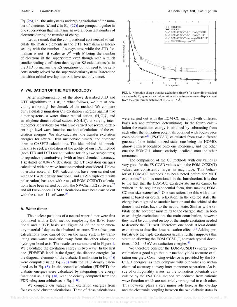
The nuclear positions of a neutral water dimer were firstoptimized with a DFT method employing the BP86 func-tional and a TZP basis set. Figure S1 of the supplemen-tary material77 depicts the obtained structure. The subsequentcalculations were carried out on the same system by trans-lating one water molecule away from the other along thehydrogen-bond axis. The results are summarized in Figure 1.We calculated the excitation energy in two ways. In the firstone (FDE/FDE label in the figure) the diabatic energies [orthe diagonal elements of the diabatic Hamiltonian in Eq. (4)]were computed using Eq. (28) with the FDE density calcu-lated as in Eq. (8). In the second calculation (FDE/ET) thediabatic energies were calculated by integrating the energyfunctional as in Eq. (18) with the density computed from theFDE subsystem orbitals as in Eq. (19).

We compare our values with excitation energies fromfour coupled cluster calculations. Three of these calculations

0 2 4 6 8 10 12 14R / Angstroms

0

0.5

1

1.5

2

Exc

itat

ion

Ene

rgy

(eV

)

FDE/FDEFDE/ETEOM-CCSD(T)/6-311G(d,p)/ROHFEOM-CCSD(T)/6-311G(d,p)/UHFEOM-CCSD(T)/aug-cc-pVDZ/ROHFFS-CCSD/aug-cc-pVDZ

FIG. 1. Migration charge-transfer excitations (in eV) for water dimer radicalcation in the Cs symmetric configuration with an intermonomer displacementfrom the equilibrium distance of 0 < R < 15 Å.

were carried out with the EOM-CC method (with differentbasis sets and reference determinant). In the fourth calcu-lation the excitation energy is obtained by subtracting fromeach other the ionization potentials obtained with Fock-Spacecoupled-cluster78 [FS-CCSD] calculated from two differentguesses of the initial ionized state: one being the HOMO,almost entirely localized onto one monomer, and the otherone the HOMO-1, almost entirely localized onto the othermonomer.

The comparison of the CC methods with our values isvery good for the FS-CCSD values while the EOM-CCSD(T)values are consistently larger in magnitude. This behav-ior of EOM-CC methods has been noted before for MCTexcitations49 and, as mentioned in the Introduction, it is dueto the fact that the EOM-CC excited-state ansatz cannot bewritten in the regular exponential form, thus making EOM-CC non-size extensive.43 One can rationalize this with an ar-gument based on orbital relaxation. In the excited state, thecharge has migrated to another location and the orbital of thedonor must relax back to the neutral state. Similarly, the or-bitals of the acceptor must relax to the charged state. In bothcases single excitations are the main contribution, howeverthey must be computed on top of the single excitation neededto describe the CT itself. Therefore, one needs at least doubleexcitations to describe these relaxation effects.32 Adding per-turbatively the triple excitations usually further improves thissituation allowing the EOM-CCSD(T) to reach typical devia-tions of 0.1–0.3 eV on excitation energies.49

We therefore consider the EOM-CCSD(T) energy over-estimation a good sign that our method yields accurate exci-tation energies. Convincing evidence is provided by the FS-CCSD energies, as they compare with our values to withinchemical accuracy at every inter-monomer separation. An is-sue of orthogonality arises, as the ionization potentials cal-culated by the FS-CCSD method are deduced from cationicwave function which are not strictly orthogonal to each other.This however, plays a very minor role here, as the overlapand the electronic coupling between the two diabatic states is

This article is copyrighted as indicated in the article. Reuse of AIP content is subject to the terms at: http://scitation.aip.org/termsconditions. Downloaded to IP:

95.130.38.103 On: Fri, 11 Apr 2014 16:48:11

054101-8 Pavanello et al. J. Chem. Phys. 138, 054101 (2013)

almost zero as proved by our calculations of S12 in Tables S1and S2 of the supplementary material.77

For sake of completeness, in the supplementarymaterial77 we report the numerical values used to obtain theplot in Figure 1 as well as additional FDE calculations carriedout with the BLYP functional showing a similar behavior tothe PW91 calculations.

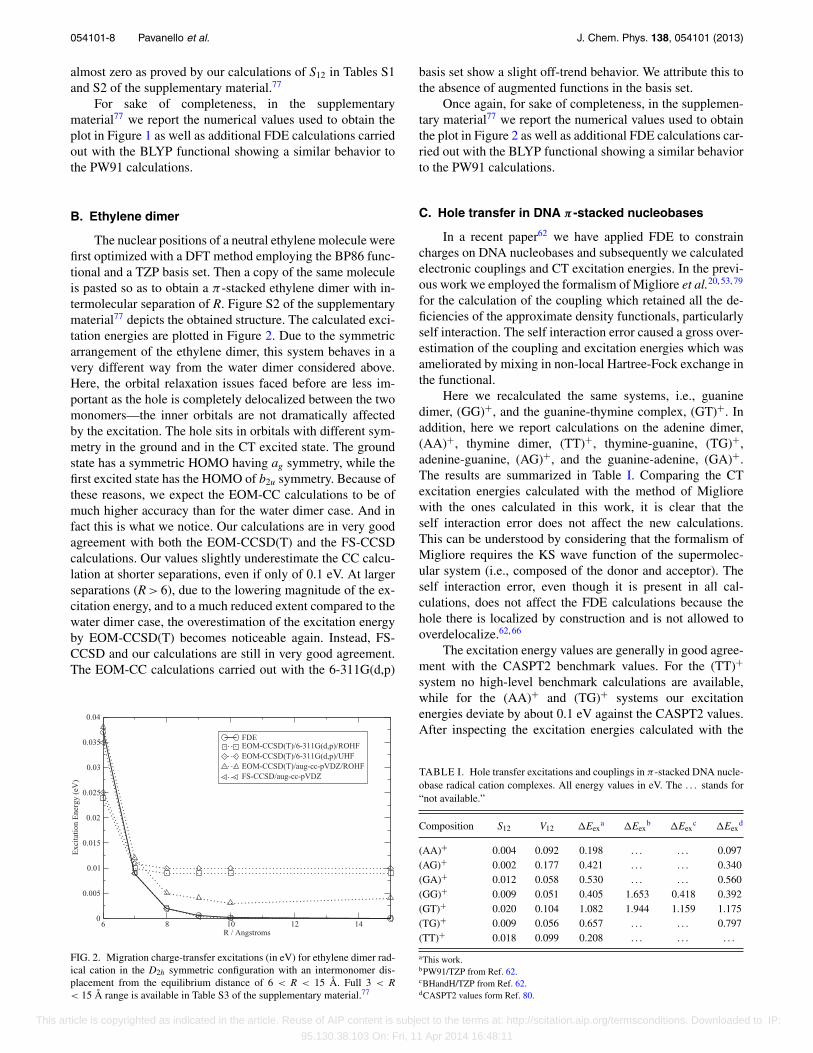
B. Ethylene dimer

The nuclear positions of a neutral ethylene molecule werefirst optimized with a DFT method employing the BP86 func-tional and a TZP basis set. Then a copy of the same moleculeis pasted so as to obtain a π -stacked ethylene dimer with in-termolecular separation of R. Figure S2 of the supplementarymaterial77 depicts the obtained structure. The calculated exci-tation energies are plotted in Figure 2. Due to the symmetricarrangement of the ethylene dimer, this system behaves in avery different way from the water dimer considered above.Here, the orbital relaxation issues faced before are less im-portant as the hole is completely delocalized between the twomonomers—the inner orbitals are not dramatically affectedby the excitation. The hole sits in orbitals with different sym-metry in the ground and in the CT excited state. The groundstate has a symmetric HOMO having ag symmetry, while thefirst excited state has the HOMO of b2u symmetry. Because ofthese reasons, we expect the EOM-CC calculations to be ofmuch higher accuracy than for the water dimer case. And infact this is what we notice. Our calculations are in very goodagreement with both the EOM-CCSD(T) and the FS-CCSDcalculations. Our values slightly underestimate the CC calcu-lation at shorter separations, even if only of 0.1 eV. At largerseparations (R > 6), due to the lowering magnitude of the ex-citation energy, and to a much reduced extent compared to thewater dimer case, the overestimation of the excitation energyby EOM-CCSD(T) becomes noticeable again. Instead, FS-CCSD and our calculations are still in very good agreement.The EOM-CC calculations carried out with the 6-311G(d,p)

6 8 10 12 14R / Angstroms

0

0.005

0.01

0.015

0.02

0.025

0.03

0.035

0.04

Exc

itat

ion

Ene

rgy

(eV

)

FDEEOM-CCSD(T)/6-311G(d,p)/ROHFEOM-CCSD(T)/6-311G(d,p)/UHFEOM-CCSD(T)/aug-cc-pVDZ/ROHFFS-CCSD/aug-cc-pVDZ

FIG. 2. Migration charge-transfer excitations (in eV) for ethylene dimer rad-ical cation in the D2h symmetric configuration with an intermonomer dis-placement from the equilibrium distance of 6 < R < 15 Å. Full 3 < R< 15 Å range is available in Table S3 of the supplementary material.77

basis set show a slight off-trend behavior. We attribute this tothe absence of augmented functions in the basis set.

Once again, for sake of completeness, in the supplemen-tary material77 we report the numerical values used to obtainthe plot in Figure 2 as well as additional FDE calculations car-ried out with the BLYP functional showing a similar behaviorto the PW91 calculations.

C. Hole transfer in DNA π-stacked nucleobases

In a recent paper62 we have applied FDE to constraincharges on DNA nucleobases and subsequently we calculatedelectronic couplings and CT excitation energies. In the previ-ous work we employed the formalism of Migliore et al.20, 53, 79

for the calculation of the coupling which retained all the de-ficiencies of the approximate density functionals, particularlyself interaction. The self interaction error caused a gross over-estimation of the coupling and excitation energies which wasameliorated by mixing in non-local Hartree-Fock exchange inthe functional.

Here we recalculated the same systems, i.e., guaninedimer, (GG)+, and the guanine-thymine complex, (GT)+. Inaddition, here we report calculations on the adenine dimer,(AA)+, thymine dimer, (TT)+, thymine-guanine, (TG)+,adenine-guanine, (AG)+, and the guanine-adenine, (GA)+.The results are summarized in Table I. Comparing the CTexcitation energies calculated with the method of Migliorewith the ones calculated in this work, it is clear that theself interaction error does not affect the new calculations.This can be understood by considering that the formalism ofMigliore requires the KS wave function of the supermolec-ular system (i.e., composed of the donor and acceptor). Theself interaction error, even though it is present in all cal-culations, does not affect the FDE calculations because thehole there is localized by construction and is not allowed tooverdelocalize.62, 66

The excitation energy values are generally in good agree-ment with the CASPT2 benchmark values. For the (TT)+

system no high-level benchmark calculations are available,while for the (AA)+ and (TG)+ systems our excitationenergies deviate by about 0.1 eV against the CASPT2 values.After inspecting the excitation energies calculated with the

TABLE I. Hole transfer excitations and couplings in π -stacked DNA nucle-obase radical cation complexes. All energy values in eV. The . . . stands for“not available.”

Composition S12 V12 �Eexa �Eex

b �Eexc �Eex

d

(AA)+ 0.004 0.092 0.198 . . . . . . 0.097(AG)+ 0.002 0.177 0.421 . . . . . . 0.340(GA)+ 0.012 0.058 0.530 . . . . . . 0.560(GG)+ 0.009 0.051 0.405 1.653 0.418 0.392(GT)+ 0.020 0.104 1.082 1.944 1.159 1.175(TG)+ 0.009 0.056 0.657 . . . . . . 0.797(TT)+ 0.018 0.099 0.208 . . . . . . . . .

aThis work.bPW91/TZP from Ref. 62.cBHandH/TZP from Ref. 62.dCASPT2 values form Ref. 80.

This article is copyrighted as indicated in the article. Reuse of AIP content is subject to the terms at: http://scitation.aip.org/termsconditions. Downloaded to IP:

95.130.38.103 On: Fri, 11 Apr 2014 16:48:11

054101-9 Pavanello et al. J. Chem. Phys. 138, 054101 (2013)

progression CASSCF(7,8), CASSCF(11,12), andCASPT2(11,12) in Ref. 80 for the (AA)+ and (TG)+

systems we notice that while for all the other nucleobasestacks the excitation energies calculated with the threemethods are similar to each other, the cases of (AA)+ and(TG)+ stand out. For example, the CASSCF(7,8) excitationenergies are 0.144 eV and 1.235 eV for the (AA)+ and (TG)+

systems, respectively. Then these values drop to 0.047 eVand 1.097 eV for the CASSCF(11,12) and then back up to0.097 eV for the (AA)+ system but go down to 0.797 eV for(TG)+ in the CASPT2 calculation.

According to Blancafort and Voityuk,80 these large fluc-tuations in the excitation energy are to be expected especiallywhen going from CASSCF to CASPT2. However, they alsonotice that for the (AA)+ system a larger active space thanthey employed should be considered to confirm the couplingsand excitation energies for this nucleobase dimer complex.Therefore, it is difficult to compare the excitation energies forall the nucleobase stacks we compute here with the CASSCFand CASPT2 calculations of Blancafort and Voityuk.80 Fur-ther analysis of these calculations (i.e., study the effect of thesize of the active space in the CASSCF/CASPT2) lie beyondthe scope of this work.

VI. PILOT CALCULATIONS: EMBEDDING EFFECTSIN WATER AND ETHYLENE CLUSTERS

In this section we present calculations carried out for sys-tems composed of more than 2 subsystems. As pilot studieswe choose the same small dimer systems considered aboveand embed them in clusters of the same molecule. First weconsider the hole transfer in ethylene dimer embedded in anethylene matrix, then we consider a water dimer in a clusterextracted from liquid water.

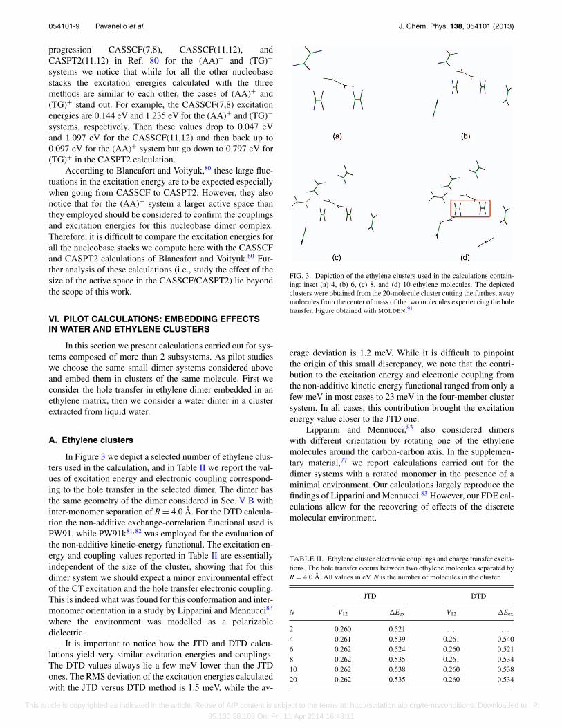
A. Ethylene clusters

In Figure 3 we depict a selected number of ethylene clus-ters used in the calculation, and in Table II we report the val-ues of excitation energy and electronic coupling correspond-ing to the hole transfer in the selected dimer. The dimer hasthe same geometry of the dimer considered in Sec. V B withinter-monomer separation of R = 4.0 Å. For the DTD calcula-tion the non-additive exchange-correlation functional used isPW91, while PW91k81, 82 was employed for the evaluation ofthe non-additive kinetic-energy functional. The excitation en-ergy and coupling values reported in Table II are essentiallyindependent of the size of the cluster, showing that for thisdimer system we should expect a minor environmental effectof the CT excitation and the hole transfer electronic coupling.This is indeed what was found for this conformation and inter-monomer orientation in a study by Lipparini and Mennucci83

where the environment was modelled as a polarizabledielectric.

It is important to notice how the JTD and DTD calcu-lations yield very similar excitation energies and couplings.The DTD values always lie a few meV lower than the JTDones. The RMS deviation of the excitation energies calculatedwith the JTD versus DTD method is 1.5 meV, while the av-

FIG. 3. Depiction of the ethylene clusters used in the calculations contain-ing: inset (a) 4, (b) 6, (c) 8, and (d) 10 ethylene molecules. The depictedclusters were obtained from the 20-molecule cluster cutting the furthest awaymolecules from the center of mass of the two molecules experiencing the holetransfer. Figure obtained with MOLDEN.91

erage deviation is 1.2 meV. While it is difficult to pinpointthe origin of this small discrepancy, we note that the contri-bution to the excitation energy and electronic coupling fromthe non-additive kinetic energy functional ranged from only afew meV in most cases to 23 meV in the four-member clustersystem. In all cases, this contribution brought the excitationenergy value closer to the JTD one.

Lipparini and Mennucci,83 also considered dimerswith different orientation by rotating one of the ethylenemolecules around the carbon-carbon axis. In the supplemen-tary material,77 we report calculations carried out for thedimer systems with a rotated monomer in the presence of aminimal environment. Our calculations largely reproduce thefindings of Lipparini and Mennucci.83 However, our FDE cal-culations allow for the recovering of effects of the discretemolecular environment.

TABLE II. Ethylene cluster electronic couplings and charge transfer excita-tions. The hole transfer occurs between two ethylene molecules separated byR = 4.0 Å. All values in eV. N is the number of molecules in the cluster.

JTD DTD

N V12 �Eex V12 �Eex

2 0.260 0.521 . . . . . .4 0.261 0.539 0.261 0.5406 0.262 0.524 0.260 0.5218 0.262 0.535 0.261 0.53410 0.262 0.538 0.260 0.53820 0.262 0.535 0.260 0.534

This article is copyrighted as indicated in the article. Reuse of AIP content is subject to the terms at: http://scitation.aip.org/termsconditions. Downloaded to IP:

95.130.38.103 On: Fri, 11 Apr 2014 16:48:11

054101-10 Pavanello et al. J. Chem. Phys. 138, 054101 (2013)

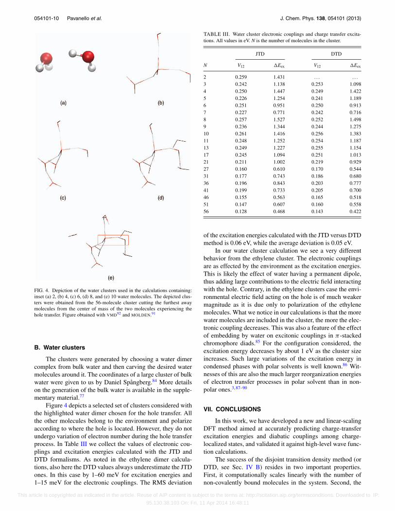
FIG. 4. Depiction of the water clusters used in the calculations containing:inset (a) 2, (b) 4, (c) 6, (d) 8, and (e) 10 water molecules. The depicted clus-ters were obtained from the 56-molecule cluster cutting the furthest awaymolecules from the center of mass of the two molecules experiencing thehole transfer. Figure obtained with VMD92 and MOLDEN.91

B. Water clusters

The clusters were generated by choosing a water dimercomplex from bulk water and then carving the desired watermolecules around it. The coordinates of a large cluster of bulkwater were given to us by Daniel Spångberg.84 More detailson the generation of the bulk water is available in the supple-mentary material.77

Figure 4 depicts a selected set of clusters considered withthe highlighted water dimer chosen for the hole transfer. Allthe other molecules belong to the environment and polarizeaccording to where the hole is located. However, they do notundergo variation of electron number during the hole transferprocess. In Table III we collect the values of electronic cou-plings and excitation energies calculated with the JTD andDTD formalisms. As noted in the ethylene dimer calcula-tions, also here the DTD values always underestimate the JTDones. In this case by 1–60 meV for excitation energies and1–15 meV for the electronic couplings. The RMS deviation

TABLE III. Water cluster electronic couplings and charge transfer excita-tions. All values in eV. N is the number of molecules in the cluster.

JTD DTD

N V12 �Eex V12 �Eex

2 0.259 1.431 . . . . . .3 0.242 1.138 0.253 1.0984 0.250 1.447 0.249 1.4225 0.226 1.254 0.241 1.1896 0.251 0.951 0.250 0.9137 0.227 0.771 0.242 0.7168 0.257 1.527 0.252 1.4989 0.236 1.344 0.244 1.27510 0.261 1.416 0.256 1.38311 0.248 1.252 0.254 1.18713 0.249 1.227 0.255 1.15417 0.245 1.094 0.251 1.01321 0.211 1.002 0.219 0.92927 0.160 0.610 0.170 0.54431 0.177 0.743 0.186 0.68036 0.196 0.843 0.203 0.77741 0.199 0.733 0.205 0.70046 0.155 0.563 0.165 0.51851 0.147 0.607 0.160 0.55856 0.128 0.468 0.143 0.422

of the excitation energies calculated with the JTD versus DTDmethod is 0.06 eV, while the average deviation is 0.05 eV.

In our water cluster calculation we see a very differentbehavior from the ethylene cluster. The electronic couplingsare as effected by the environment as the excitation energies.This is likely the effect of water having a permanent dipole,thus adding large contributions to the electric field interactingwith the hole. Contrary, in the ethylene clusters case the envi-ronmental electric field acting on the hole is of much weakermagnitude as it is due only to polarization of the ethylenemolecules. What we notice in our calculations is that the morewater molecules are included in the cluster, the more the elec-tronic coupling decreases. This was also a feature of the effectof embedding by water on excitonic couplings in π -stackedchromophore diads.85 For the configuration considered, theexcitation energy decreases by about 1 eV as the cluster sizeincreases. Such large variations of the excitation energy incondensed phases with polar solvents is well known.86 Wit-nesses of this are also the much larger reorganization energiesof electron transfer processes in polar solvent than in non-polar ones.3, 87–90

VII. CONCLUSIONS

In this work, we have developed a new and linear-scalingDFT method aimed at accurately predicting charge-transferexcitation energies and diabatic couplings among charge-localized states, and validated it against high-level wave func-tion calculations.

The success of the disjoint transition density method (orDTD, see Sec. IV B) resides in two important properties.First, it computationally scales linearly with the number ofnon-covalently bound molecules in the system. Second, the

This article is copyrighted as indicated in the article. Reuse of AIP content is subject to the terms at: http://scitation.aip.org/termsconditions. Downloaded to IP:

95.130.38.103 On: Fri, 11 Apr 2014 16:48:11

054101-11 Pavanello et al. J. Chem. Phys. 138, 054101 (2013)

hole transfer excitation energies calculated with mainstreamGGA-type functionals reproduce within chemical accuracycalculations carried out with several types of coupled clus-ter methods. For the benchmark cases considered, our methodoutperforms the biased EOM-CCSD(T), while it is in excel-lent agreement with vertical ionization potential differencescalculated with Fock-Space CCSD calculations. We also car-ried out calculations of the hole transfer excitations in sevenDNA base pair combinations reproducing CASPT2(11,12)calculations within a 0.1 eV deviation or better. Pilot calcu-lations on molecular clusters of water and ethylene have alsobeen carried out with cluster sizes up to 56 molecules. Weshow how the method is able to recover solvation effects ondiabatic couplings and site energies (needed in electron trans-fer calculations) as well as the excitation energies at the dis-crete molecular level and fully quantum-mechanically. Thisconstitutes an important step forward in the development oflinear scaling electronic structure methods tailored to electrontransfer phenomena.

Future improvements of the method are underway andwill include the implementation of hybrid functionals in thepost-SCF calculation of the full-electron Hamiltonian ma-trix elements and the extension of the method to both ex-citations involving charge separation and covalently boundsubsystems.

ACKNOWLEDGMENTS

We are indebted to Daniel Spångberg for providingus with the water cluster structures. We also acknowledgeBenjamin Kaduk for helpful tips for coding of the transitiondensity, and Alexander Voityuk for helpful discussions. M.P.acknowledges partial support by the start-up funds providedby the Department of Chemistry and the office of the Deanof FASN, Rutgers-Newark. J.N. is supported by a VIDI grant(Grant No. 700.59.422) of the Netherlands Organization forScientific Research (NWO).

1V. May and O. Kühn, Charge and Energy Transfer Dynamics in MolecularSystems (Wiley-VCH, 2011).

2A. M. Kuznetsov and J. Ulstrup, Electron Transfer in Chemistry and Biol-ogy (Wiley-VCH, 1998).

3A. Nitzan, Chemical Dynamics in Condensed Phases (Oxford UniversityPress, Oxford, 2006).

4L. L. Miller, Y. Yu, E. Gunic, and R. Duan, Adv. Mater. 7, 547 (1995).5G. Inzelt, Conducting Polymers (Springer, New York, 2008).6L. G. Reuter, A. G. Bonn, A. C. Stückl, B. He, P. B. Pati, S. S. Zade, andO. S. Wenger, J. Phys. Chem. A 116, 7345 (2012).

7H. B. Gray and J. R. Winkler, Annu. Rev. Biochem. 65, 537 (1996).8T. Kawatsu and D. N. Beratan, Chem. Phys. 326, 259 (2006).9E. Romero, M. Mozzo, I. H. M. van Stokkum, J. P. Dekker, R. vanGrondelle, and R. Croce, Biophys. J. 96, L35 (2009).

10G. D. Scholes, G. R. Fleming, A. Olaya-Castro, and R. van Grondelle, Nat.Chem. 3, 763 (2011).

11A. J. Storm, J. van Noort, S. de Vries, and C. Dekker, Appl. Phys. Lett. 79,3881 (2001).

12B. Giese, Acc. Chem. Res. 33, 631 (2000).13J. C. Genereux and J. K. Barton, Chem. Rev. 110, 1642 (2010).14B. Kaduk, T. Kowalczyk, and T. Van Voorhis, Chem. Rev. 112, 321 (2012).15T. Van Voorhis, T. Kowalczyk, B. Kaduk, L.-P. Wang, C.-L. Cheng,

and Q. Wu, Annu. Rev. Phys. Chem. 61, 149 (2010).16C.-P. Hsu, Acc. Chem. Res. 42, 509 (2009).17G. Hong, E. Rosta, and A. Warshel, J. Phys. Chem. B 110, 19570 (2006).18R. J. Cave and M. D. Newton, J. Chem. Phys. 106, 9213 (1997).

19J. E. Subotnik, J. Vura-Weis, A. J. Sodt, and M. A. Ratner, J. Phys. Chem.A 114, 8665 (2010).

20A. Migliore, J. Chem. Phys. 131, 114113 (2009).21M. E. Casida, “Time-dependent density functional response theory for

molecules,” in Recent Advances in Density Functional Methods Part I,edited by D. P. Chong (World Scientific, Singapore, 1995), pp. 155–192.

22A. Dreuw and M. Head-Gordon, Chem. Rev. 105, 4009 (2005).23O. Gritsenko and E. J. Baerends, J. Chem. Phys. 121, 655 (2004).24J. Neugebauer, O. Gritsenko, and E. J. Baerends, J. Chem. Phys. 124,

214102 (2006).25J. Plotner, D. J. Tozer, and A. Dreuw, J. Chem. Theory Comput. 6, 2315

(2010).26T. Yanai, D. P. Tew, and N. C. Handy, Chem. Phys. Lett. 393, 51 (2004).27J. Toulouse, F. Colonna, and A. Savin, Phys. Rev. A 70, 062505 (2004).28I. C. Gerber and J. G. Angyan, Chem. Phys. Lett. 415, 100 (2005).29E. Livshits and R. Baer, J. Phys. Chem. A 112, 12789 (2008).30R. Baer, E. Livshits, and U. Salzner, Ann. Rev. Phys. Chem. 61, 85

(2010).31T. Ziegler and M. Krykunov, J. Chem. Phys. 133, 074104 (2010).32J. E. Subotnik, J. Chem. Phys. 135, 071104 (2011).33A. Dreuw, J. L. Weisman, and M. Head-Gordon, J. Chem. Phys. 119, 2943

(2003).34A. Dreuw and M. Head-Gordon, J. Am. Chem. Soc. 126, 4007 (2004).35J. Autschbach, ChemPhysChem 10, 1757 (2009).36S. Grimme and F. Neese, J. Chem. Phys. 127, 154116 (2007).37C. Hättig, “Structure optimizations for excited states with correlated

second-order methods: CC2 and ADC(2),” in Advances in Quantum Chem-istry (Elsevier, 2005), Vol. 50, pp. 37–60.

38A. D. Dutoi and L. S. Cederbaum, J. Phys. Chem. Lett. 2, 2300 (2011).39A. J. A. Aquino, D. Nachtigallova, P. Hobza, D. G. Truhlar, C. Haettig, and

H. Lischka, J. Comput. Chem. 32, 1217 (2011).40A. I. Krylov, Acc. Chem. Res. 39, 83 (2006).41J. F. Stanton and R. J. Bartlett, J. Chem. Phys. 98, 7029 (1993).42J. F. Stanton, J. Chem. Phys. 101, 8928 (1994).43M. Musial and R. J. Bartlett, J. Chem. Phys. 134, 034106 (2011).44B. M. Wong and J. G. Cordaro, J. Chem. Phys. 129, 214703 (2008).45T. Stein, L. Kronik, and R. Baer, J. Am. Chem. Soc. 131, 2818 (2009).46T. Stein, L. Kronik, and R. Baer, J. Chem. Phys. 131, 244119 (2009).47C. Hättig, A. Hellweg, and A. Köhn, J. Am. Chem. Soc. 128, 15672

(2006).48C. Hättig and F. Weigend, J. Chem. Phys. 113, 5154 (2000).49K. R. Glaesemann, N. Govind, S. Krishnamoorthy, and K. Kowalski, J.

Phys. Chem. A 114, 8764 (2010).50G. te Velde, F. M. Bickelhaupt, E. J. Baerends, S. J. A. van Gisbergen, C.

Fonseca Guerra, J. G. Snijders, and T. Ziegler, J. Comput. Chem. 22, 931(2001).

51C. R. Jacob, J. Neugebauer, and L. Visscher, J. Comput. Chem. 29, 1011(2008).

52M. D. Newton, Chem. Rev. 91, 767 (1991).53A. Migliore, J. Chem. Theory Comput. 7, 1712 (2011).54F. Plasser and H. Lischka, J. Chem. Phys. 134, 034309 (2011).55S. Efrima and M. Bixon, Chem. Phys. 13, 447 (1976).56Y. Mo and S. D. Peyerimhoff, J. Chem. Phys. 109, 1687 (1998).57E. Gianinetti, M. Raimondi, and E. Tornaghi, Int. J. Quantum Chem. 60,

157 (1996).58A. A. Voityuk and N. Rösch, J. Chem. Phys. 117, 5607 (2002).59Q. Wu and T. Van Voorhis, J. Chem. Phys. 125, 164105 (2006).60T. Kubar, P. B. Woiczikowski, G. Cuniberti, and M. Elstner, J. Phys. Chem.

B 112, 7937 (2008).61A. A. Voityuk, J. Jortner, M. Bixon, and N. Rösch, J. Chem. Phys. 114,

5614 (2001).62M. Pavanello and J. Neugebauer, J. Chem. Phys. 135, 234103 (2011).63T. A. Wesolowski and A. Warshel, J. Phys. Chem. 97, 8050 (1993).64P. Cortona, Phys. Rev. B 44, 8454 (1991).65T. A. Wesolowski, “One-electron equations for embedded electron density:

Challenge for theory and practical payoffs in multi-level modeling of com-plex polyatomic systems,” in Computational Chemistry: Reviews of Cur-rent Trends, edited by J.Leszczynski (World Scientific, Singapore, 2006),Vol. 10, pp. 1–82.

66A. Solovyeva, M. Pavanello, and J. Neugebauer, J. Chem. Phys. 136,194104 (2012).

67S. Fux, C. R. Jacob, J. Neugebauer, L. Visscher, and M. Reiher, J. Chem.Phys. 132, 164101 (2010).

68M. Iannuzzi, B. Kirchner, and J. Hutter, Chem. Phys. Lett. 421, 16 (2006).

This article is copyrighted as indicated in the article. Reuse of AIP content is subject to the terms at: http://scitation.aip.org/termsconditions. Downloaded to IP:

95.130.38.103 On: Fri, 11 Apr 2014 16:48:11

054101-12 Pavanello et al. J. Chem. Phys. 138, 054101 (2013)

69A. J. W. Thom and M. Head-Gordon, J. Chem. Phys. 131, 124113 (2009).70I. Mayer, Simple Theorems, Proofs, and Derivations in Quantum Chem-

istry, Mathematical and Computational Chemistry (Kluwer Academic/Plenum, 2003), Chap. 5.

71A. Farazdel, M. Dupuis, E. Clementi, and A. Aviram, J. Am. Chem. Soc.112, 4206 (1990).

72H. F. King, R. E. Stanton, H. Kim, R. E. Wyatt, and R. G. Parr, J. Chem.Phys. 47, 1936 (1967).

73R. McWeeny, Methods of Molecular Quantum Mechanics (Academic, SanDiego, 1992).

74A. Götz, S. Beyhan, and L. Visscher, J. Chem. Theory Comput. 5, 3161(2009).

75M. Valiev, E. Bylaska, N. Govind, K. Kowalski, T. Straatsma, H. V. Dam,D. Wang, J. Nieplocha, E. Apra, T. Windus, and W. de Jong, Comput. Phys.Commun. 181, 1477 (2010).

76DIRAC, a relativistic ab initio electronic structure program, Releasedirac11, 2011, written by R. Bast, H. J. Aa. Jensen, T. Saue, and L.Visscher, with contributions from V. Bakken, K. G. Dyall, S. Dubillard,U. Ekstrm, E. Eliav, T. Enevoldsen, T. Fleig, O. Fossgaard, A. S. P. Gomes,T. Helgaker, J. K. Lrdahl, J. Henriksson, M. Ilia, Ch. R. Jacob, S. Knecht,C. V. Larsen, H. S. Nataraj, P. Norman, G. Olejniczak, J. Olsen, J. K. Peder-sen, M. Pernpointner, K. Ruud, P. Saek, B. Schimmelpfennig, J. Sikkema,A. J. Thorvaldsen, J. Thyssen, J. van Stralen, S. Villaume, O. Visser, T.Winther, and S. Yamamoto, see http://dirac.chem.vu.nl.

77See supplementary material at http://dx.doi.org/10.1063/1.4789418 for ad-ditional tables and description of the water cluster structures.

78L. Visscher, E. Eliav, and U. Kaldor, J. Chem. Phys. 115, 9720 (2001).79A. Migliore, S. Corni, D. Versano, M. L. Klein, and R. Di Felice, J. Phys.

Chem. B 113, 9402 (2009).80L. Blancafort and A. A. Voityuk, J. Phys. Chem. A 110, 6426 (2006).81T. A. Wesolowski, H. Chermette, and J. Weber, J. Chem. Phys. 105, 9182

(1996).82A. Lembarki and H. Chermette, Phys. Rev. A 50, 5328 (1994).83F. Lipparini and B. Mennucci, J. Chem. Phys. 127, 144706 (2007).84D. Spangberg, Uppsala University, private communication (2012).85J. Neugebauer, C. Curutchet, A. Munoz-Losa, and B. Mennucci, J. Chem.

Theory Comput. 6, 1843 (2010).86B. Mennucci, Theor. Chem. Acc. 116, 31 (2006).87R. Gutiérrez, R. A. Caetano, B. P. Woiczikowski, T. Kubar, M. Elstner, and

G. Cuniberti, Phys. Rev. Lett. 102, 208102 (2009).88R. Seidel, M. Faubel, B. Winter, and J. Blumberger, J. Am. Chem. Soc.

131, 16127 (2009).89J. Blumberger and G. Lamoureux, Mol. Phys. 106, 1597 (2008).90M. Pavanello, L. Adamowicz, M. Volobuyev, and B. Mennucci, J. Phys.

Chem. B 114, 4416 (2010).91G. Schaftenaar, MOLDEN3.7—A pre- and post processing program of

molecular and electronic structure, CMBI, the Netherlands, 2001.92W. Humphrey, A. Dalke, and K. Schulten, J. Mol. Graphics 14, 33 (1996).

This article is copyrighted as indicated in the article. Reuse of AIP content is subject to the terms at: http://scitation.aip.org/termsconditions. Downloaded to IP:

95.130.38.103 On: Fri, 11 Apr 2014 16:48:11