AN ABSTRACT OF THE THESIS OF

Donald John Baumgartner for the Doctor of Philosophy

(Name) (Degree)

m Civil Engineering presented on ___M_a_y~-l_l_l967___ (Major) (Date)

Title VERTICAL JET DIFFUSION IN NON LINEAR DENSITY

STRATIFIED FLUID

Abstract approved

The simplified equations of motion proposed by Morton to deshy

termine the extent of vertical travel of a forced plume in a linear

density stratified environment were re-written and solved in a way

which allowed them to be applied to any non linear profile of density

For application to any specific situation it was shown that the solution

did not have to commence from a virtual point source but rather

could start from the actual source of finite diameter progressing in

steps through a number of segments of variable length In each segshy

menta linear density gradient was specified which closely approxishy

mated the actual gradient A method was developed to find the virtushy

al point source however for those cases requiring the comparison

of flows in a linear gradient

The equations of motion provided a method for achieving simishy

larity between model and prototype and this method was employed in

designing the physical model studies incorporated in this study

Experimental values of maximum penetration and of the posishy

tion of the horizontally-spreading layer were obtained in a one meter

deep tank of 2 4 meters diameter Stratification was obtained with

salt solutions of varying densities The results from runs using five

different gradients and the results of analyzing the experiments of

others demonstrated that the method is suitable for obtaining a rough

approximation of the location of the bottom of the horizontal layer

Its use for estimating maximum penetration is discounted on both

theoretical grounds and experimental evidence Both levels were unshy

derestimated by the mathematical model in comparison to the exshy

perimental values

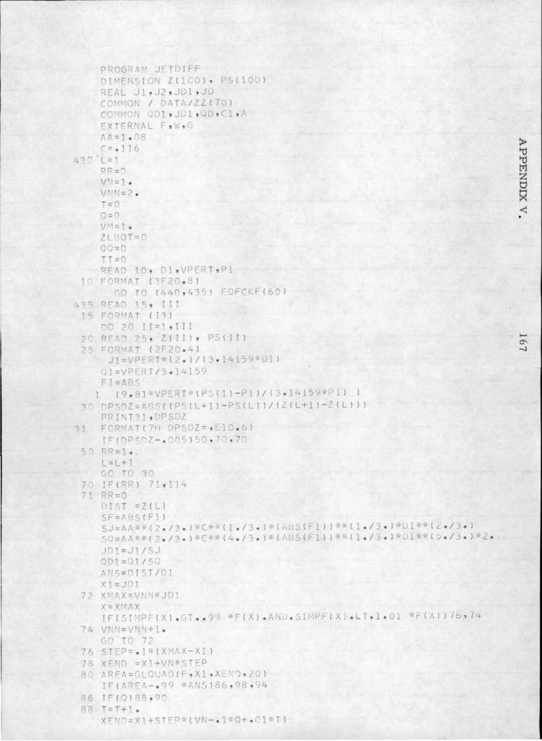
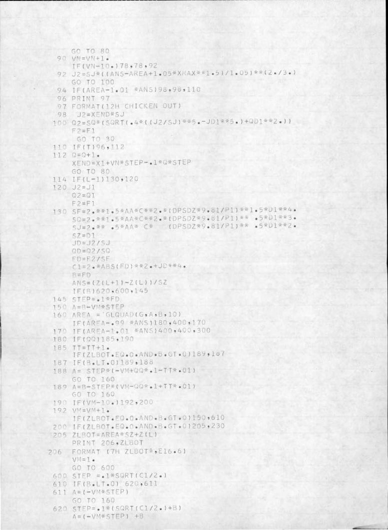
A computer program was employed to solve the equations and

rounding errors as well as inefficient methods of quadrature were

found to account for as much as forty percent of the discrepancy beshy

tween observed and predicted values

Vertical Jet Diffusion in Non Linear Density Stratified Fluid

by

Donald John Baumgartner

A THESIS

submitted to

Oregon State University

in partial fulfillment of the requirements for the

degree of

Doctor of Philosophy

June 1967

APPROVED

Professor of Civil Engineering

Dean of Graduate School

Date thesis is presented May 11 1967 ----------~--~--~~-----------------

Typed by C 1 o ve r R e dfe r n f o r ____DonaldJohnBau=mg2artn-=-=e-=r--shy

ACKNOWLEDGEMENT

The writer is indebted to the Federal Water Pollution Control

Administration and to Dr Leon W Weinberger of that organization

for complete financial support for the program of research reported

herein

Appreciation is expressed for the guidance and support receiveJ

from Dr D C Phillips Professor F J Burgess and Dr L S

Slotta of the Department of Civil Engineering and for the financial

support for computer services received from Dr D D Aufenkamp

Director of the Computer Center Oregon State University Helpful

suggestions and encouragement were received from Leale E Streebin

during the course of this study and should be acknowledged Thanks

are also due to Mrs Maureen Gruchalla for her patience in typing

the first draft of the manuscript

Finally the dedication perseverance confidence and enshy

couragement of the authors wife Therese and their children were

essential to the successful completion of this program and are grateshy

fully and sincerely appreciated

TABLE OF CONTENTS

Page

I INTRODUCTION 1 Mixing of Stratified Reservoirs 1 Improving the Design 3 The Problem to be Solved 4 Fundamentals and Definitions 5

II PREVIOUS INVESTIGATIONS 7

Flow Into Density Stratified Fluid (Linear

Initial Independent Variation of Buoyancy

Development of the Theory 7 Lanltina r Jet 7 Turbulent Jet (No Buoyancy) 9 Turbulent Plume (No Momentum) 21

Gradient) 24

and Momentum 27 Extension of Thea ry 48

III PROPOSED IMPROVEMENT 85 Normalization 85

Stratified Environment 85 Uniform Environment 96

Solution of Equations 99 Stratified Environment 99 Uniform Environment 114 Solution of Problem 115

IV MODEL STUDIES 118 Similitude 118 Experiments 120

Mathematical Arrangement 120 Physical Arrangement 121

V RESULTS AND ANALYSIS OF DATA 130

VI DISCUSSION OF RESULTS 136

VII CONCLUSIONS 145

BIBLIOGRAPHY 147

APPENDIX Appendix I Appendix II Appendix III Appendix IV Appendix V

Page

157 157 159 160 162 167

LIST OF TABLES

Table Page I Hydraulic characteristics of experimental runs 126

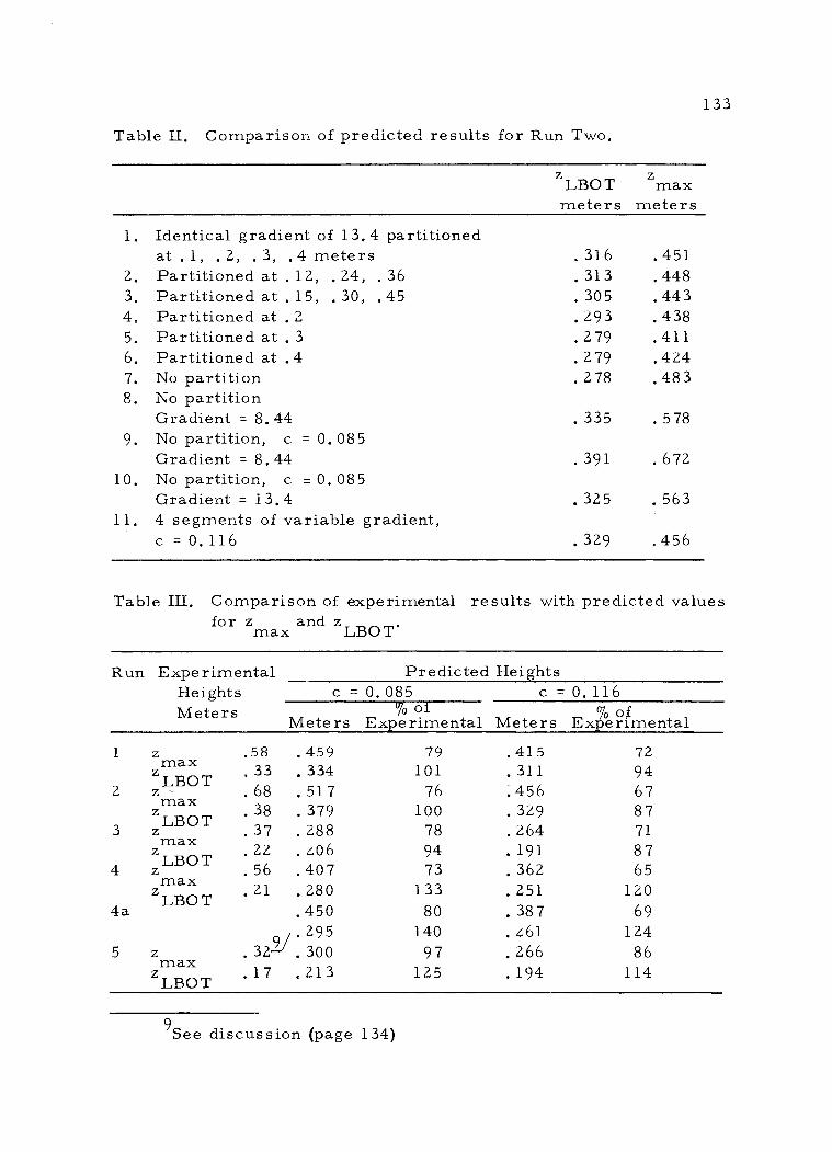
II Comparison of predicted results for Run Two 133

Ill Comparison of experimental results with predicted

values for zmax and zLBOT 133

IV Observes and predicted values of Hart 1 s experiments 140

VERTICAL JET DIFFUSION IN NON LINEAR DENSITY STRATIFIED FLUID

I INTRODUCTION

Jet diffusion is involved in at least three currently important

problems confronting sanitary engineers (1) dispersion of liquid

wastes from outfall sewers (2) dispersion of stack gases into the atshy

mosphere and (3) mixing of density stratified impoundments The

first two are well known and their relationships to the theoretical

study of jet diffusion has long been established The third problem

has many interesting facets only a portion of which can be investigatshy

ed via the same theory Because this is a relatively new application

additional background information may prove valuable

Mixing of Stratified Reservoirs

Frequently storage capacity is included in multi-purpose reshy

servoirs for downstream water quality control but unfortunately

this storage in itself may impair quality To combat this mechanical

mixing has been employed and is currently considered among the passhy

sible methods of quality control For a general discussion of this

problem the reader is referred to Symons Weibel and Robeck (1964)

Mechanical mixing has also been used to prevent or remove ice forshy

mations from reservoir surfaces and these applications provide the

2

bulk of the technical documents available on the subject

The physical nature of a reservoir which causes the problem to

develop is related primarily to the density-temperature function of

water which allows a body of water to become density stratified under

the influence of solar energy and wind induced surface currents

Hutchinson (1957) gives a good presentation of the physics of stratifishy

cation and the types of density-depth profiles which have been found

They are customarily non-linear Of secondary importance at least

in fresh water impoundments is the density gradient induced by the

varying concentratwn of dis solved salts

Returning to the cases where m1xing has been employed eight

tests have been reviewed in which diffused air was employed at rates

ranging from 0 03 to 3 cubic feet per minute per acre foot (cfmAF)

of volume One test (Patriarche 1961) in which the aeration rate

was between 0 06 and 0 08 cfmAF was unsuccessful while the others

were considered successful Although the data are incomplete it apshy

peared that the higher rates were associated with shorter operating

times hence the energy inputs per unit volume were not as widely

separated as the rates Several attempts at mixing have also been

made using pumps to transfer cold water from the hypolimnion to the

warm epilimnion where when discharged from a pipe mixing occurs

by jet diffusion However sufficient data for comparison of energy

requirements are not available The point to be made is that these

3

devices are be1ng used and considered for additional use in spite of

the fact that nowhere has a rational or fundamental basis for such a

design been set forth

Improving the Design

It seems only reasonable that the size of the reservoir the deshy

gree of stratification the power of the device and the time it 1s to

operate are involved in the design

The items of power and time have two limits imposed on them shy

an economic and a natural limit If it turns out that an energy expendshy

iture of X horsepower-hours (Hp-hrs) is required to reduce the

stratification a certain amount this can be achieved with any set of

values for power and time such that their product equals X Howshy

ever a massive pump which would operate for a short time would not

necessarily be the most economical arrangement since its first cost

would be extremely high and its unit operating cost would be low On

the other extreme it is realized that the natural forces causing stratshy

ification operate on a cycle somewhat less than annual and hence any

small pump requiring an ope rating time greater than this is naturally

unacceptable

Many choices are available to the engineer and to narrow down

the discussion only vertically oriented devices will be considered

further even though devices discharging horizontally are occasionally

4

used in this practice

Whether discharging from a line source or a point source when

a vertical device is used the degree to which stratification is changed

by mixing can be related to the volurne flux and the location of the

horizontally spreading mixed layer In addition to location the vela-

city of the spreading layer is important since high velocities encourshy

age additional entrainment by vertical mixing across the density

boundary Abraham (1963) provided additional comments on this

These parameters can be related to conditions at the terminashy

tion of a zone of vertical jet diffusion A rational basis of pump or

aerator selection will be provided if the required terminal condishy

tions can be related to the physical source variables and the density

gradient in the fluid For a single point source these variables would

be the jet or orifice diameter D the velocity of discharge vJ J

the initial density difference between the jet fluid and the receiving

fluid 6p l

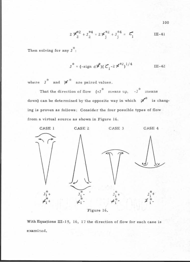
The Problem to be Solved

Before approaching the problem of optimizing the selection of

input devices it is first necessary to be able to relate the input varshy

iable s to conditions at the onset of the horizontally spreading layer

At present as the literature review will show these relationships

are not available By assuming a completely quiescent ambient fluid

5

the problem is greatly simplified Abraham (1963) has given an apshy

proximate solution to the basic portion of this problem but the speshy

cifically desired answers are not readily available This study will

be an attempt to solve specifically for

1 The maximum height reached by a forced plume

2 the initial volume flux in the horizontally spreading mixed

layer

3 the location of the horizontally spreading mixed layer

The solution is to be sought for the case of a single circular source

Fundamentals and Definitions

In elementary fluid mechanics practical solutions to problems

are frequently found by idealizing the flow to neglect friction Detershy

mining the trajectory of a jet of water in air and the coefficient of

contraction for flow from a Borda mouthpiece are examples of fruitshy

ful utilization of ideal flow approximations Unfortunately when a

liquid jet is discharged into a liquid this simplification can no longer

be accepted due to the important action of viscous friction Preservshy

ing the simplifications of steady incompressible flow with no velocity

fluctuations (laminar) fluid motion can be described by means of the

Navier- Stokes equations The net force of gravity is cancelled when

both liquids are of the same density and by specifying additionally

that no angular component of velocity exists (two dimensional

6

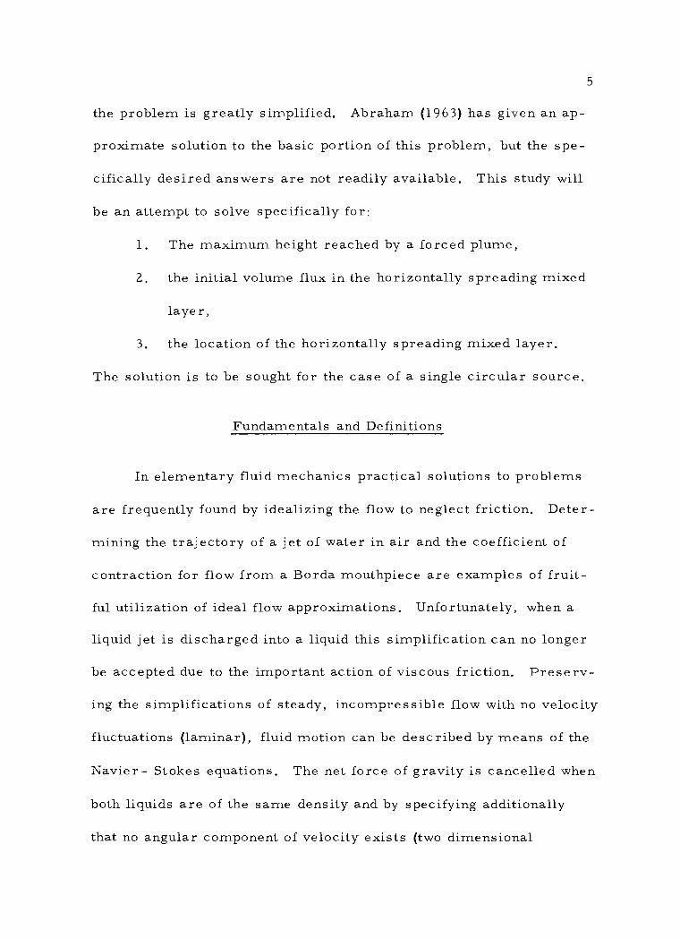
axisymmetric) the equations of motion are written as

2 2 v ov v ov a v ov v a v

r r z r aP r 1 r r r + = + v(-- +--- -- +--) I-1or oz p or 2 2 ~ 2or r or r uz

2 2 v OV v ov ~ a v av a v

r z z z uP z 1 z z + =--tv(--+--+--) I-2or oz ar 2 az 2 paz r or

The equation of continuity for these specifications is

ov v ov r r z+-+--=0 I- 3or r az

The symbol v represents the kinematic viscosity P the presshy

sure and the other symbols are defined in Figure l

v z

With this fundamental theoretical

background early investigators

attempted to develop a theory to

describe the nature of jet diffushy

sian

Figure 1

7

II PREVIOUS INVESTIGATIONS

Development of the Theory

Laminar Jet

When a fluid is discharged through a circular orifice into an inshy

finitely large expanse of similar fluid at rest fluid is entrained from

z the s tationa ry fluid due to visshy

cous forces The downstream

velocity is decreased as more

and more fluid partakes in the

flow Although the affected area

ideally extends to r = plusmnoo for

some arbitrarily small value of

v the horizontal distance z

r at which v is obtained 0 z

describes a line (on an axial

plane) whose equation is

nFigure 2 r = Y]Z bull In 1 9 3 3 Schlichting

0

(1960) gave an exact solution for this type of problem by assuming

(1) that the pressure in the main direction of flow was nearly conshy

stant (2) the velocity in the r direction was everywhere small

compared to that in the z direction (3) that the spatial rate of

r

8

change of v is much greater in the radial than in the longitudinalz

direction The latter two assumptions are the essence of the boundshy

ary layer approximations which had been recently advanced to solve

flow problems involving solid boundaries (Schlichting 1960 page 109)

Their use in free boundary flows as in jet diffusion and wakes was

only now emerging By comparing the order of magnitude of the terms

involved in Equation I-2 (Schlichting 1960 page 182) he showed that

o2 v oz 2

could be neglected giving z

ov ov ~ ov z z 1 u z v -- + v = v--(r-) II-1

z oz r or r or or

Similarly he showed that all the terms of I-1 were insignificant comshy

pared to II-1 and could be neglected entirely The key to the solution

was in the next assumption that the velocity profile was of constant

form at all sections It is this assumption which characterizes a

group known as similarity solutions Knowing or assuming the

flow at some section say the orifice provided the boundary condishy

tion of K the kinematic momentum flux

2 K = 2rr f v z rdr II-2

0

which is constant

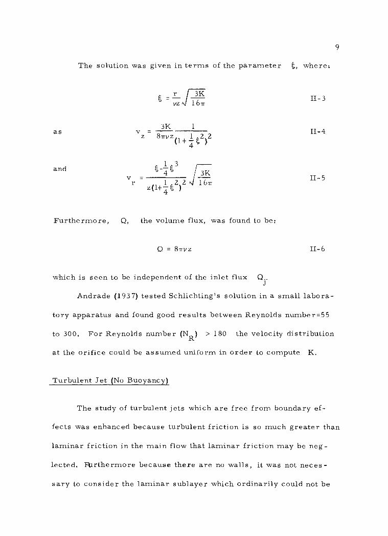
9

The solution was given in terms of the parameter ~ where

t - ~[Ks - II-3 vz 161T

3K 1 as v = II-4

z 81TVZ(lt __ ~2)2 4

and v = II- 5

r

Fur thermo re 0 the volume flux was found to be

0 = 81TVZ II-6

which is seen to be independent of the inlet flux 0 J

Andrade (1937) tested Schlichting 1s solution in a smalllaborashy

tory apparatus and found good results between Reynolds number=55

to 300 For Reynolds number (NR) gt 180 the velocity distribution

at the orifice could be assumed uniform in order to compute K

Turbulent Jet (No Buoyancy)

The study of turbulent jets which are free from boundary efshy

fects was enhanced because turbulent friction is so much greater than

laminar friction in the main flow that laminar friction may be negshy

lected FUrthermore because there are no walls it was not necesshy

sary to consider the laminar sublayer which ordinarily could not be

10

neglected Since the observed nature of turbulent jet dispersion exshy

hibited similar characteristics to the laminar jet namely (a) the exshy

tent of lateral flow involvement was small compared to the longitudishy

nal extent and (b) the lateral gradients of velocity were much greater

than those in the main direction of flow the use of Prandtl s boundshy

ary layer approximations again allowed a 2 v oz 2

to be neglected z

as well as the equation for the r direction Consequently the

equations of motion were written in identical form as for the laminar

case ie

2a--v av a v av z z z 1 z

v +v = E (-- +--) II-7 z oz r or T or r or

where the overbar designates the time average In solving this equashy

tion simultaneously with the continuity equation (Equation l-3) which

remains unchanged it was necessary to ernploy assumtions regardshy

ing based on empirical evidence Prandtl s mixing length thea-ET

ry was successfully employed for this purpose (Schlichting 1960 p

591) Although normally expressed as

Il-8

Prandtl also hypothesized a relationship for free stream turbulence

(as a jet) which expressed ET as proportional to the width of the

mixing zone and velocity fluctuations in the transverse direction ie

ll

= cr v II-9 o r

where the prime designates the fluctuating component Additional

evidence extended this to include the dependence of v on r

hence

= c r v Il-l 0 1 o zltt

He used the similarity assumption with n = 1 hence

r 0

and thus

= c zv 3 zltt II-11

For the laminar jet and supported by empirical evidence of turbulent

jets

then

II-12

a constant

Employing ET as a constant the situation was entirely analoshy

gous to the laminar case where v was a constant and the results

were (the time average quantities designated above by the overbar

as v are henceforth represented without the overbar) z

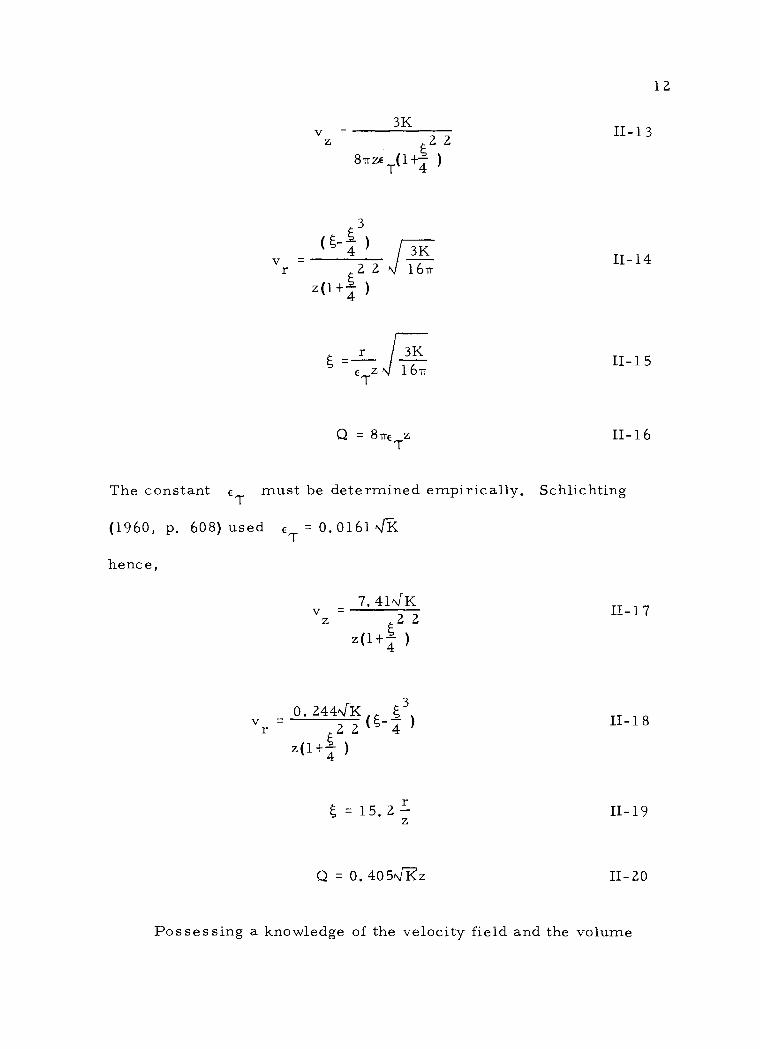
12

v z

3 (~-1 )

4 v =--0_2_2_ f[f

r

z(l + )

~ __r_ ~ -e zJ~ T

Q = 8Tie z T

The constant e must be determined empiricallyT

(1960 p 608)used E =00161-KT

hence

7 41-JK v =

z ~ 2 2 z(l +4 )

3 v = 0 244fK (~-5_ )

r ~ 2 2 4 z(l +4 )

r ~ = 15 2shy

z

Q = 0 405-JKz

II-13

II-14

II-15

II-16

Schlichting

II-1 7

II-18

II-19

II-20

Possessing a knowledge of the velocity field and the volume

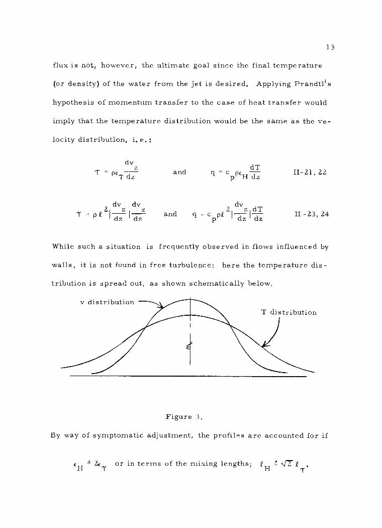
13

flux is not however the ultimate goal since the final temperature

(or density) of the water from the jet is de sired Applying Prandtl1 s

hypothesis of momentum transfer to the case of heat transfer would

imply that the temperature distribution would be the same as the veshy

locity distribution ie

dv z dT

T = pe -shy and q = c pe - II-2122T dz p H dz

dv dv dv2 z z 2 z dT

T = ppound ~~~~ and q = c ppound 1-1- II- 23 24 p dz dz

While such a situation is frequently observed in flows influenced by

walls it is not found in free turbulence here the temperature disshy

tribution is spread out as shown schematically below

v distribution

Figure 3

By way of symptomatic adjustment the profil~s are accounted for if

- 2e or in terrns of the mixing lengths 7 pound T T

14

There is however a theoretical justification for this result based

on Taylors (1915) vorticity transfer theory which assumes that a

two dimensional eddy conserves its vorticity The theory predicts

the sarne value of eddy viscosity as Prandtls theory and hence leads

an 1d t ve 1oc1ty d butlon- l T 1 (1932) d escr1 h1sto en 1ca1 1str1 ay or bes t

theory and its differences from Prandtls momentum transfer theory

in a very straightforward n1anner and then shows that for heat transshy

fer his theory predicts a temperature distribution (adjusted for coinshy

cidence of maximums) which is the square root of the velocity distrishy

bution or that EH = 2E T The experin1ental studies of Fage and Falshy

kner (1932) and according to Schlichting (1960) those of Reichardt

(1942-not seen 1944) show good agreement for this result The disshy

tribution equations are not given here since they pertain to plane (two

dimensional) flow

The extension of the vorticity transport theory seemed a naturshy

a1 step but as Taylor (1935) pointed out the resulting equations are

useless due to their complication unless simplifying assumptions

are made A special type of 3 dimensional flow - that exhibiting symshy

metry around an axis - reduces the equations to a type containing two

This is actually a special case of two dimensional flow and the only one where the results would be similar Here the turbulence in the direction of flow can be neglected and turbulence can be considshyered to be restricted to the coordinate transverse to the direction of flow In other two dimensional cases where the longitudinal turbushylence cannot be neglected the results are different

1

15

coordinates and is one such assumption Taylor then assumed that

the nature of the turbulence is such that the components of vorticity

are transferred without change to a new position and the eddy retains

these components until mixing occurs with the surroundings The use

of this assumption constitutes the modified vorticity transport theshy

ory

Goldstein (1935) simplified the general theory for axisymmetric

flows by assuming in addition that the turbulence was symmetric

about the same axis

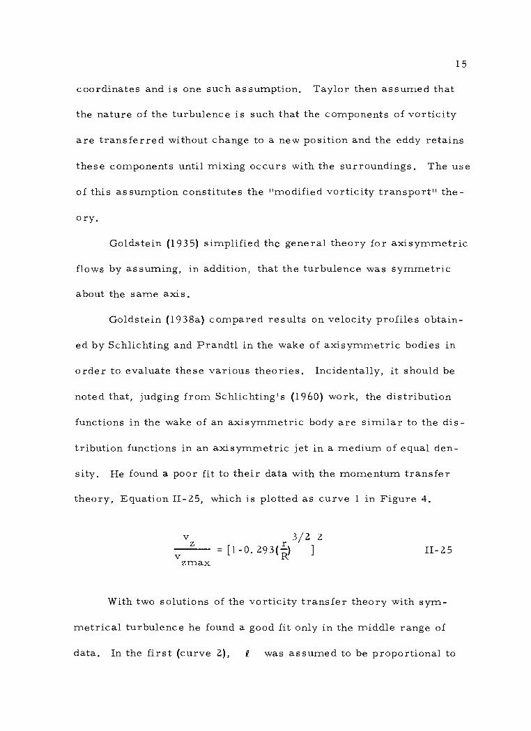
Goldstein (l938a) compared results on velocity profiles obtainshy

ed by Schlichting and Prandtl in the wake of axisymmetric bodies in

order to evaluate these various theories Incidentally it should be

noted that judging from Schlichtings (1960) work the distribution

functions in the wake of an axisymmetric body are similar to the disshy

tribution functions in an axisymmetric jet in a medium of equal denshy

sity He found a poor fit to their data with the momentum transfer

theory Equation II-25 which is plotted as curve 1 in Figure 4

v 32 2 z

=[l-0293(~ ] II-25 v

zmax

With two solutions of the vorticity transfer theory with symshy

metrical turbulence he found a good fit only in the middle range of

data In the first (curve 2) pound was assumed to be proportional to

v

II- 26

16

1r as shown in Equation II- 26

v 4 r 52 18 r 52 1 r 152z = 1-s-ltmiddot 863R_) + 1 75( 863 R) +I 225 ( 863R) +

zmax

v z

v zmax

1 A -----shy ~

8

Curve Z

6

4

L

5 rR

] r_) z

l

Curve 4

Figure 4

ThisIn the second solution (Curve 3) was presun1ed

equation was

v 3 z z

[1-0 Z93(i) ] II- 27 v

zmax

Using the nwdified vorticity transfer theory resulted in curve 4

Equation II- 28

v z 1 4 r 3 2 14 r 3 7 r 9Z

v =3[3-31225R) +81(1225R)- 6561(1225R) - ] zmax

II-28

17

v zmax

=

r 0

v

Figure 5

From Goldsteins text of the

experimental procedure the

schematic description shown

in Figure 5 was deduced as

zrnax an aid in describing the 2

terms In regard to the temshy

perature distribution Gold-

stein had no experimentally obtained data to compare against so he

plotted the four curves and mentioned that none seemed to be satisshy

factory This result is shown later in Figure 6

Curve 1 is _T_T__ = (1-0 293(~)32]2 Il-29 max

as for v v and z zmax

TCurve 2 is II-30

T max

Curve 3 is T =1-0 293(~) 3 II- 31

T max

which is the square root of v vz zmax

18

Curve 4 is

In Equation II- 30

and

T T

max

11 1

= 0 863rR

II-32

In Equation II-32

and

11 1

= 1 2 2 5 r R

19

1

Curve 2~ 8

Curve 3T T 6 max

4 Curve 4Curve

2

r -~ 1 15 2 25 rR

Figure 6

Each of the above equations employs R which is considered proporshy

tional to r which in turn is proportional to z 0

Howarth (1938) following the work of Goldstein (19 38a) carried

out the derivation of the formulae for the most pertinent case of the

axisymmetric jet and compared it with the work of Tollmien (1945)

and of Ruden (1933) The results for the cases of axially symmetric

turbulence appear to the author as no better than Goldsteins 1 while

the cases of momentum transfer theory (Tollmien) and the vorticity

transfer theory seem to apply satisfactorily Unless Howarth had

Rudens original data not much confidence can be placed in a comshy

parison based on the graphs shown in the published work (Ruden 1933

20

since the scale is very small and no data points are plotted -merely

a curve Furthermore the equations are left in a cumbersome form

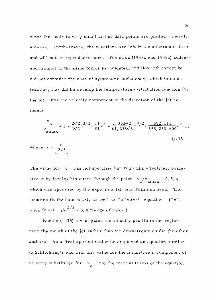
and will not be reproduced here Tomotika (1938a and 1938b) addresshy

sed himself to the same topics as Goldstein and Howarth except he

did not consider the case of symmetric turbulence which is no deshy

traction nor did he develop the temperature distribution function for

the jet For the velocity component in the direction of the jet he

iound

v z 2J 2 31 2 1 1 3 1 363J2 92 592111 6 v = 1 - 3J 3 l + 8l l 61236J3l +3582306001 -

zmax

II- 33 r

where l = --shy23

c z

The value for c was not specified but Tomotika effectively evalushy

ated it by forcing his curve through the point v jv = 0 5 l z zmax

which was specified by the experimental data Tollmien used The

equation fit the data nearly as well as Tollmien 1s equation (Tollshy

23mien found 1c = 34 edge of wake)

Kuethe (1935) investigated the velocity profile in the region

near the mouth of the jet rather than far downstream as did the other

authors As a first approximation he employed an equation similar

to Schlichting 1s and with this value for the mainstream component of

velocity substituted for v into the inertial terms of the equationz

21

of motion he solved for v in the frictional term The integrashyz

tion was constrained so that the profiles of the first and second apshy

proximations were coincident at the edge of the mixing region and at

the boundary of the core The final equations are not convenient to

reproduce here What is important was his experimental verificashy

tion - both of his work and of Tollmiens His solution very accrushy

ately predicted the velocity distribution out to about 4 4 diameters

and Tollmien s was accurate after 9 3 diameters He showed that a

central core existed whose center line velocity was maintained conshy

stant at the center line velocity in the orifice for 4 4 diameters doWilshy

stream and that the profile was changed from essentially rectangushy

lar to the typical jet profile in that distance

Turbulent Plume (No Momentum)

W Schmidt (1941) added to the more complete understanding of

the case of diffusion of an axisymmetric heated jet by considering the

case of no initial 1nomentum the motion being caused by the buoyanshy

cy associated with a heat induced density difference (The resulting

mixing region in this case is frequently called a plume) Using the

assumptions of similarity of profiles constant heat flux and a mixshy

ing length = cz he showed that

= f (I])Z -13v II- 34 z 1

22

f (ll)z -53 II-35 2

The functions of ll were given in a series expansion Rouse apshy

parently unaware that Schmidt had solved the problem also reported

(Rouse Yih Humphreys 1952) on the case of buoyancy only Howshy

ever he employed slightly different assumptions Rouse used boundshy

ary layer type approximations for the equations of motion and assumshy

ed that pgtgt6 p as well as the mixing length form of the eddy diffushy1

sian factor The result of these simplifications was that the axial

gradient of momentum flux was found to be equal to the buoyancy of a

transverse layer of unit thickness Then assuming similarity at all

transverse sections he showed that

r II- 36

cz

-l3 II-37vz ~ z

-53= g6p I( z II-38

53Q eKtz II-39

43K cz II-40

13G cltz II-41

where G is the unit buoyant force

23

II-42

where W = source output of weight deficiency or flux of incremental

weight

Note here that W is constant along the axial direction whereas

with the jet K was

He then employed dimensional analysis to establish

v z = f ( z r p W)1

and

tsy = f (z r p W)2

and then in accordance with his analytical development he set

v z r = f (-) II-43

3 z

and

ty w2 13

ltEf-gt

= r f (-)4 z

II-44

z

To fully express the functional relationship it was necessary to asshy

sume some form of profile and to fit his experimental results he

chose the Gaussian function Incidently he first showed that NR

5for turbulent mixing could be set at 10 and the height z at

E

which the plume became turbulent was

24

II-45

where W was evaluated from

W = - gqc T II-46 p

using the approximation that

6T - - II-47

T

Finally he found

v z

II-48

2 13 2 2 = _11 ( p (- W) ] e - 7 1 r z II-496 5

z

II- 50

Flow Into Density Stratified Fluid (Linear Gradient)

Batchelor (1954) in a very readable lecture Y reviewed the

problem pointing out explicitly how 6y comes to be considered as

a variable Using purely a dimensional argument with the aid of the

similarity principle he arrived at the same form as Rouse Yih and

2 Although not a part of the problem here considered it is worthshy

while to note that Batchelor mentions an unpublished work of G I Tayshy

lors asserting the identical flow regime from a line sourc~ of air bubbl~c as for a line sourc~ of heat

25

Humphreys (19 52) He cons ide red the mixing length argument of

Schmidt (1941) as an unsatisfactory approach and presumably thereshy

fore also Rouse 1 s He then extended his argun1ent to the case of a

buoyant plume in an unstable stratified surrounding fluid He claimed

similarity solutions do not exist for a stable environment a frequent

occurrence in the atmosphere

Priestley and Ball (1955) however assumed similarity of proshy

files and found the same form of solution with respect to z but

containing also aT oz They found a solution for the case where s

v and tsy could be assumed to follow the same Gaussian profile z

(requiring an experimentally evaluated constant)

For neutral conditions ie aT oz = 0 s

3 3 13D~ D v-3W J J ]v = II- 512 (l- 2 2) +z 3 3

2Tic p z 4c z 8c z

2 D 3 3 -l3-WT D v 6T = ~--s-[ -3W (l- j ) + J J ] II- 52

2 2 2 4 2 2 3 3 Tig p C Z 21TC p Z C Z 8c z

The choice of the term v 1s this writer 1 s Priestley having employshyJ

ed the value of v ie v at z = z where equals thezV z v

height above the origin (virtual source) Similarly D is employed J

rather than 2r at z = z The substitution seems to be suggestive0 v

of a more general solution where there is initial momentum

Before considering the case of thermal stratification they

26

suggested forming dimensionless quantities v and z from z

-middotshybullbull

v = v vz z zgt

= ( )13-3where 21TC p Z

hence 1-v~d l3

II-53n ] z z

From this it is seen that the fluid will accelerate upward if

gt~ 3 v lt 23 and will decelerate upwards otherwise

J

With aT az positive Priestley and Balls solution can be s

solved numerically but not analytically The method involves the

condition that aT I az is independent of z and zaT az is efshys s

fectively constant They developed a dimensionless measure of strashy

tification 2 defined as

3 zv IaTamp=lt---s)ll4 II- 54

2 T az

where

T = II-55

and then

II- 56 dz

27

For the case where v = 0 a substitution allowed further simplifi-J

cation and prediction of a ceiling height

Initial Independent Variation of Buoyancy and Momentum

Morton Taylor and Turner (1956) used a slightly different apshy

proach to the problem They assumed that the effects of turbulence

cause the rate of inflow to the plume at the edge of the plume to be

related to some characteristic velocity in the plume at that height an

assumption first employed by Taylor in 1945 (Taylor 1945) This

amounts to saying

o(Q-Q)J = f(v ) II-57 oz z

It was noted that similarity solutions were not entirely acceptable

since the situation predicted is obviously violated where the plume

spreads out horizontally They too pointed out that a pertinent varishy

able is (ps-p)g the buoyant force per unit volume The source

strength however must be referred to some chosen density when a

density gradient exists in the fluid They chose at z = zV i e Ps

To proceed with their analysis they selected as the secshy

tion velocity representative of the turbulent entrainment phenomenon

and further assumed similarity of profiles at each section (in the low-

e r portion of the plume at least) and that the local variations in denshy

sity are small compared to the reference density The solution is

28

carried out for op oz linear identical Gaussian profiles for s

v z and 6 p zV = 0 and K = 0 at z = 0 thus the solution reshy

quires that the problem is reduced to describing the flow from a virshy

tual point source caused by buoyancy only By making the change of

variables

J = r v II-- 58 0 z

22_ = r v II- 59

0 z

2W r v ~ and II-60

0 z p

4 = -gdps II- 61 p dz

sV

and then making dimensionless ratios

II-62

II-63

where c is the entrainment coefficient or rather the ratio of enshy

trainment velocity to the centerline velocity

29

1T 12 1I 4 1ZJ _ 4 Psv

J -- II-64 234W 34

1

278 14 12_8 14 1T c psV z

z

= II-65 w_14

1

The generalized equations gave rning the motion are

d~-middot- lt --_ = J II-66 dz

II-67

II-68-shy_

dz

_

The boundary conditions are when z

= 0

J

0

lt _

= 0

These equations were integrated numerically from z = 0 to 0 9

and from 0 9 to 2 8 by a finite difference method the first terms repshy

resenting the solution to W Schmidts problem The vanishing of

30

v J ~2 bull bull

= J ~ when z = z 28 corresponds to the maximum z max

plume height At z = 2 125 6p vanishes To express their reshy

sults in terms of v r and 6y they used z 0

38 14 bull rag Psv 1

r = - II-69 0 1 2 1 4 bull0 82c w J

1

0 86 12 14 v c p v J2 z s

v = II-70 z W14J8 ~-middot-

1

12 o 61c g6ecy = II-71 58 34w 14

-41 Psv i

They speculated that the thickness of the mixed horizontal layer will

be h

= 2 8 = 2 1 = 0 7 and that the distance above the source to

the center of this layer z~ = 2 45 Figure 7 below shows howshy

ever that 6Y and v become increasingly large near the source z

which is due only to the mathematical nature of the solution

From the defining equation for z ~

rearranging gives

14 gt~ 041W z

1 z =------------shy II-72

12 38 14 c 4 psV

In their experimental results they assumed z was 2 8 hence max

31

1

T 14 l 15 vi

z II-73 = ( 12 14)(-3--~max c Psv J

W and ) as well as p being known z was compared~ sV max

14W

with ( 1

) with excellent results In evaluating cr wasjj 38 0

l chosen as the value of r for which hence r =Oll2zv z = -vz4_ 0

and c = 0 093 (For This Result See Appendix I)

In the above analysis z was v taken as zero but the experimenshy3

tal data showed a slope intersectshy

ing the z axis at -5 2 em when

z = 0 was taken at the actual

z source The authors then sugshy

gested selecting an 11 effective 1

r 11 r equal to r when

~ o eo 6

l v = -- v and allowing this

z 100 z

point to coincide with In1Dr D

this case then zV =fa = 5 Scm

(See Appendix II) and they concluded that the measurement for z

should be made from the virtual source In other words the actual

D source is at z = __L bull

48

F H Schmidt (19 57) remarked that Priestley and Balls solution

l 2 3

Figure 7

32

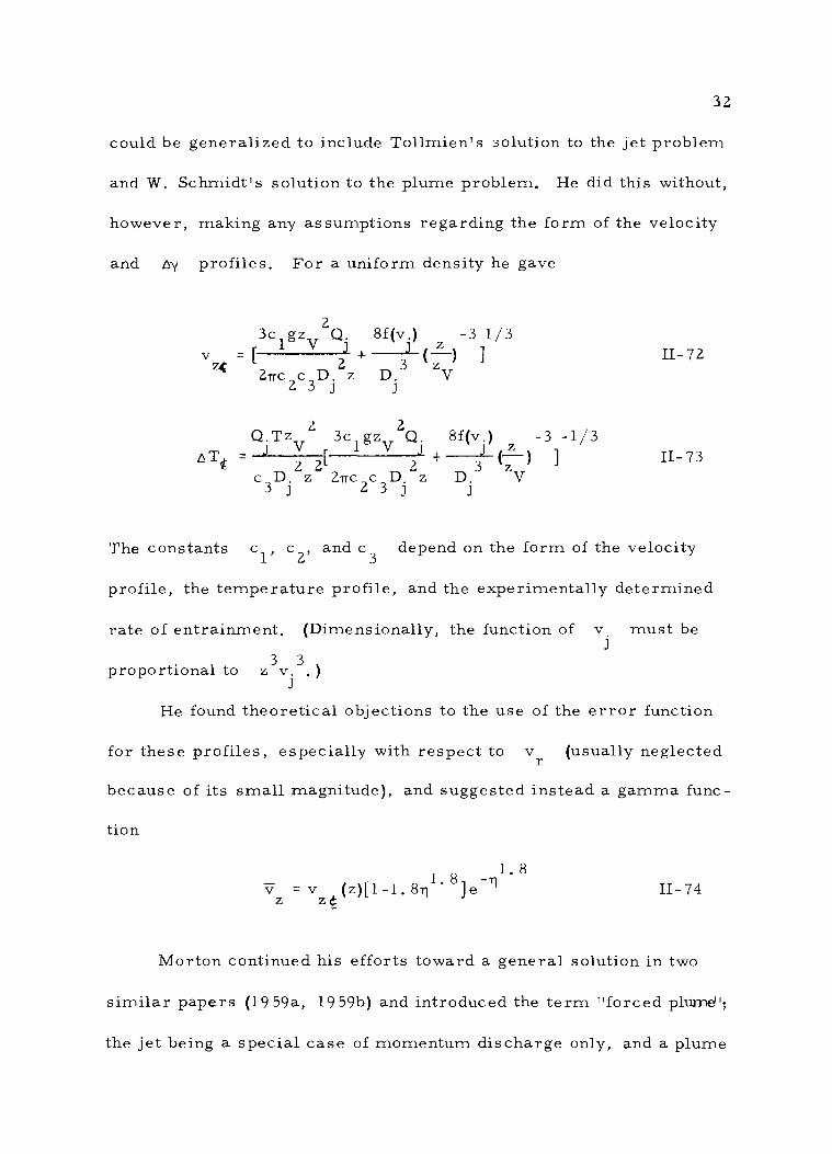
could be generalized to include Tollmien 1 s solution to the jet problen1

and W Schmidts solution to the plume problem He did this without

however making any assumptions regarding the form of the velocity

and sy profiles For a uniform density he gave

2 3c gzV Q 8f(v) -3 13

1II-72v =[ l + l (-f-) ]

~ 2TTC c D z D v

2 3 J J

2 2 QjTzV 3c gzv Qj 8f(v) -3 -l3

1 = 2 2 [ 2 +_ ___3J-- lt-f-) ] II-73

c D z 2Tic c D z D V 3 J 2 3 J J

The constants c c and c depend on the form of the velocity1 2 3

profile the temperature profile and the experimentally determined

rate of entrainment (Dimensionally the function of v must be j

3 3proportional to Z V )

J

He found theoretical objections to the use of the error function

for these profiles especially with respect to v (usually neglected r

because of its small magnitude) and suggested instead a gamma funcshy

tion

1 8 - 1 8 11v =v (z)[1-l 811 middot ]e II-74

z z

Morton continued his efforts toward a general solution in two

similar papers (19 59a 19 59b) and introduced the term forced plume

the jet being a special case of momentum discharge only and a plume

33

being the special case of buoyancy only The following development

is from (1959a) unless special discussion or detail warrants refershy

ence to the other paper in which case it will be noted The nomenshy

clature for the most part is from Morton Taylor and Turner

(19 56) or from other previously used relationships Initially he forshy

malized the case for uniform surroundings when the forced plume has

either positive or negative buoyancy and positive or negative momenshy2 2

-96r ztuml He adopted Rouses (1952) profiles namely e for

-7lr 2z 2

velocity and e for the width of the profile

being Ar 0

Using

1J = r v II-75

u 0 Zf [2

2 2 A r v by

0 z$ = II-76lu 2

(l+A )psV

2 = r v II-77lu 0 zctshy

where the subscript u represents the special case for uniform

surroundings

3The sign convention now employed is this K is + if the jet is

pointed in the tz direction and wi is +if the buoyanl force acts initialshyly in the tz direction and v v It will be necessary to provide the

sign for K from inspection of the system hence plusmnK will appear in subsequent relationships however the +or - sign

1for W will appear

algebraically as a result of its definition employing the lerm (p -p) s J

34

2 II-78

The physical meanings are

TipJ momentum f1 middotlt u

= buoyancy flux II-79

Tip a = mass flux II-80 J u

2K = 1TpJ = initial momentum flux II- 81

1 J U1

w =TIP v- = initial buoyancy flux (differs II-82 1 S U1

fro1n Morton Taylor and

Turner (19 56) by a factor of 1 2)

M = TIP~ = initial mass flux II- 83 1 J U1

Mathematically discharge from a virtual source with K and W 1 1

requires M =0 hence Morton cons ide red this case first Dimenshy1

sionless quantities

J u J = II-84

u IJ ui I

J(l +A 2) I~ I f =

U U1 II-8 5

u 234cl2IJ 52

U1

234cl2zj(l+A2)jz j ~ U1

z = II-86 IJ 32

U1

35

and the fact that ~ = -fr provided the following equations of mo-U Ul

tion

II-87

= ~~ -lt II-88 bull u

dz u

The boundary conditions were

_ _

when z = 0 and J = sign J u U Ul

His solution can be simplified by limiting consideration to

sign J = + and sign f = + Ul Ul

The solution of this set is in terms of J u

36

The results were conveniently displayed graphically as

12IIgt( sy r--u 1 o

z vs --- N----------------~- ~ r u ~lt D 12 12 l2 o

J j vj psVu

ie a measure of the width of the plume and as

z vs v u zt

ie a measure of axial velocity

The graph in Figure 8 shows both the initial influence of momentum

and the ultimate influence of buoyancy

Mass Flux as Independent Variable

A more exacting solution which allowed independent variation of

the initial mass flux M from the source K W and M reshy1 1 1 1

quired consideration of the effects of the finite area of discharge

The governing differential equations were the same but the boundary

conditions became

when

z 0 J 1 u u

37

where

II-89

10

8

0lt z 6

u

4

2

I Plume jy

I _

J u

~

Forced

Plume

Jet

I I

I 4Jlt2

u ~~ _ ib u

2 4 6 lt2

4J u --_ and

J u

Figure 8

_ Now he made the important distinction that z be measured from

u

z - 0 at the actual source For analysis he said a forced plume u

which is the same above this point can be 11 generated 11 from a virtual

point source W oK located at z = -z Naturally the flow in 1 1 u Vu

38

this plume had to satisfy the same differential equations but the modshy

ified boundary conditions became

when

where

z = 0 u

at the virtual source ie

I

z = z z u u Vu

and

His solution was

II-90

= 31 5 - 11 2 lt 5 _ 5ll122 5 6 II-911 Vu

II-92

In order to have the plumes the same at z = o u

II-93

39

where

and

l

= gt10 s 5 05-l2 3d

IYvz -Vu Yv Yv

0

1I lo I

=flo lo 132 S 5 -l2 3 It -sgnol tdt

sgno

sgnamp = tl if Oltr lt l case a(Olt 6 lt l)

sgno = - l if r gt 1 case b (6 lt 0)

E-94

In case (a) above the behavior of flow is that of a source

located at

z Vu

=

l6

r1oo 3

2S ltt

5 -l)shy

1

l

2 t

3dt II-9 5

and the full solution is given for the fo reed plume (W K 0) preshy1 1

viously discussed

A special case when r = l was described as the plume (W)1

middotmiddotshyfrom a source of buoyancy only at zmiddotmiddotmiddot = 2 108 For case (b) the

Vu

forced plume behaves as though it were emitted from a virtual source

(W - lo IK 0) situated at 1 1

40

1 JoJ 32s 5 -123z =loJol (t +1) t dt II-96

Vu - 1

For r increasing above 1 the effect of initial momentum is deshy

creasing and the situation depicted of negative initial momentum can

be acceptably visualized If z ~lt

turns out to be positive the vir-Vu

tual source is above the actual source The constant c (the entrain-shy

ment ratio) was evaluated as 0 082 as described in his 1959 paper and

the constant A was evaluated as 1 16 from Rouses work (1952)

Morton referred to his 1959 paper to substantiate the statement

that the use of Gaussian profiles was unsatisfactory for solving the

flow problem when the fluid was stratified but reference to that pashy

per and to his 1956 paper provides only the argument that top hat

profiles are simpler Regardless of his reasons the solution is

developed for a forced plume with a profile of constant v across z

the width of 2r (z) and zero for r gt r and similarly for the 0 0

buoyancy g6p over the width Ar (z) Although this new profile 0

changes the value of the constants to c = 0 116 and A = 1 108 the

calculated maximum height is not affected Since this situation is

similar to the previous case where actual sources (W K M) 1 1 1

were related to virtual sources (W K 0) only the latter were 1 1

considered Also the stratification was limited to that caused by a

negative linear density gradient

41

Once again distances were measured from the origin located at

the virtual source rather than from the actual source The equations

governing the flow are

2d(r v )

0 z = lcr v II-9 7dz 0 z

2 2d( pv r )

z 0 2 2 = A gr (p -p) II-98

dz 0 s

2 d[r v (p -p)]

o z sV II-99

dz

Then substituting the left side of II-9 7 into the right side of II-99

2 d[r v (p -p)] dp

0 z s 2 s = r v II-1 00

dz 0 z dz

Equation II-98 was simplified by assuming p bull p sV = constant

which was certainly a much closer approximation than previous ones

because in the cases under consideration p gt 0 996 and psV lt l 000

becoming

2 2 d(r v )

0 z 2 2 0=A r ____ (p -p) II-101

dz o Psv s

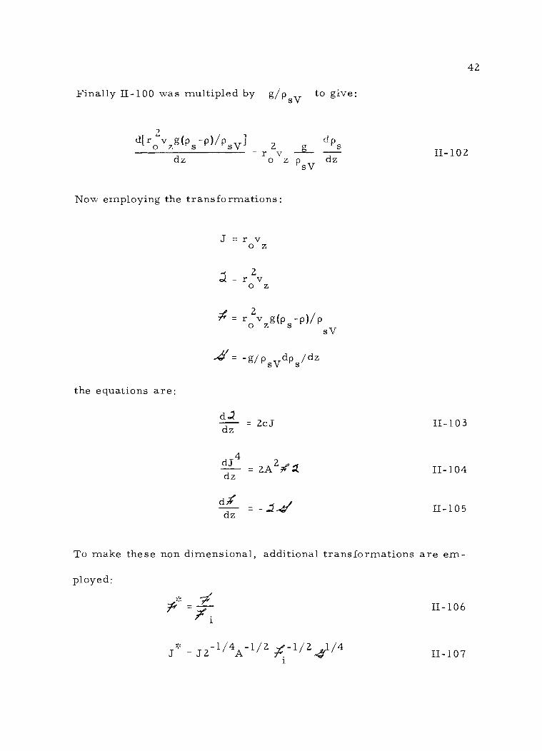
42

Finally Il-l 00 was multipled by g psV to give

d[r v g(o -p)p v]o z middots s 2

o dp

s = r v _l2_

dz o z psV dz

Now employing the trans fa rmations

J = r v 0 z

2 r v

0 z

2~ = r v g(p -p)p o z s sV

1 = - gj p dp dzsV s

the equations are

d~ = 2cJ

dz

dJ4 2 = 2A tf ~

dz

dft = - ~-41dz

To make these non dimensional additional transformations

played

= J 2 -l4A-l2 ~-l2 cent14 1

II-1 0 2

II-1 03

II-1 04

II-105

are emshy

II-106

II-107

43

~~ -518 -112 -14 _-314 58J = i 2 c A ~ d II-1 08 1

Il-l 09

Substituting these the final dimensionless equations of motion are

dt

-- = J

II-11 0 dz

4dJ -yen--t gt-- = II-111 dz

d4

= -1

II-112 dz

Boundary conditions were given as

when

z = 0

~~ - 1 14 - 1 12 - 1 12 _~) 14 = J ~J = 2 A ri -~ Ji 1

(note dependence onJ)

1~~ = f(M) = 0 1

(Zero mass flux from virtual source)

The following solution applies for the case of constant 4

44

Morton found (using II-111 and II-112 above)

l l- CY

II-11 3

where

CY=

4J4 1

2 2 4 A t~J

1 1

II-114

and

~~ ~ =

1-s l2(-)

1 - CY II-11 5

where

s = 42(1-cr)J II-116

In this case it should be noted that

J is a maximum

at the point where (~~ vanishes and becomps zero at the top of the

plume where then

___) -- -l27 -(1-CY) II-11 7

For the lower part of the plume (CY ~ s~ l) he used equations II-111

and II-112 to find

2 -l4 -34 ss l4 -l2I = 2 (1-CY) t (1-t) dt

CY

II-118

II-119

45

In the lower part (ls~O)

bull

then for 0 lt r lt 1 middot z is then found from II-111 middot max

~lt -718 -18 dtt1

z =2 (1-CY) 1 1 2

max sY (1-t) 2 ~(54 1j2t) - ~(541 2Y)

sl dt 1 2 2+ 0 (l-t) 1 2(3(514 12)- (3(514 ll2t)- (3(514 li2CY) l

II-120

For the case r lt 0

~lt 2

- 7I 8 -1 I 8 CY

cit zmax = (1-CY) j J(Tt)0f3(54 l2CY)- (3(54 l2t)

0

II-1 21

For the case r gt 1

~lt _ 2

- 7I 8 -118 CY

cit zmax- (l-CY) -SO -f(l-t)-(3(54 l2CY)-f3(54 l2t)

cl 1

+ j [ -if3(5l4 li2CY) + f3(5l4 ll2t)0

1 ] dt + - 2(3(514 112) t f3(5l4 li2CY)- f3(5l4 ll2t) -1-t

II-122

46

3

Oltrlt l

2 o

z max rlt 0

l

2 4 bull h 8 CY

Figure 9

c In Figure 9 z is plotted against 0 the value for CY = 0

max

agreeing with the previously reported 2 8 (Morton 1956) As CY

increases z gt~

decreases due to mixing near the source but at max

() = 0 8 buoyancy is becoming less in1portant than momentum

Morton made the point in both his 1959 papers that the position

of the virtual source can be found with little error by using the equashy

tions developed for the uniform environment but unfortunately he

used different expressions for r andz

inl959b u

case a (0lt 6 lt 1)

II-123

II-124

47

The above developments constituted the early attempts to desshy

cribe and verify the nature of velocity and temperature distribution in

jets It contained the germ of a theory in the starting point of the

equations of motion and continuity however to proceed from this

point toward a solution required the use of assumptions to simplify the

equations - assumptions which frequently were known by their invenshy

tors to be largely at odds with reason and with the appreciation of the

theory of turbulent motion as they visualized it (Taylor 1932) (Birkshy

hoff and Zarantonello 1957 p 304-312) They also had to make asshy

sumptions about the form of the terms remaining such as e =can-T

2 dv z n stant or E =pound and P = ex based on their observations of

T dz

the phenomena andor on their intuition This at best leaves us

with a 11 phenomenological 11 or 11semi-empirical 11 theory - frequently (if

not always) with an empirically determined value for some constant

c Their justification of course lies in their successful application

in the solution of problems which could not even be approximately solshy

ved if a wholly theoretical solution had been required Liepmann and

Laufer (1947) said 11 It is typical of phenomenological theories of turshy

bulence that the mean-speed distributions derived from such theories

can be brought into fair agreement with experimental measurements 11

and then showed that neither the mixing length nor the exchange coefshy

ficient is constant across a section of a two dimensional jet hence the

successful 11 theories were based on invalid assumptions

48

A great deal of subsequent experimental work has been reported

which refines the techniques adds simplifying assumptions or points

out areas of theoretical improvernents but which on the whole do not

contribute any new theoretical methods of treating the phenomenon of

jet dispersion This section is entitled extension of theory 11

Extension of Theory

Corrsin (1943) undertook extensive studies of temperature and

velocity profiles along diameters at axial distances of 0 to 40 diametshy

ers and compared the results with theoretical predictions according

to Tollmiens momentum transfer theory with constantpound (at each secshy

tion) with Taylors vorticity transfer with constant pound (according to

Tomotika) and with Prandtl s constant ET (formulation given by

Schlichting (1960)) Using very sophisticated hot wire anemometer

measuring and recording techniques he was able to develop valuable

data concerning the fluctuating components in the flow His conclushy

sions provided new information relative to the nature of the flow as

well as providing the most comprehensive test of theory to that time

Corrsin found that temperature diffuses more rapidly than velocity

noticeable even in the core described by Kuethe

In his studies none of the theories gave a staisfactory relationshy

ship between the spread of velocity and temperature The theoretical

curves were matched to the observed curve where the velocity equaled

49

1 one half the centerline velocity In the region from v = -v

z 2 zmax

on either side of the centerline the velocity profile resulting from

the assumption of constant fit the best For the temperature

curves the Schlichting model was not used because it required an asshy

sumption regarding the value of eH whereas the other two theories

yielded a predicted profile based only on the nature of pound If the theshy

1oretical curves were matched at v =-v both failed to pre-

z 2 zmax

diet the temperature distribution (Taylors being only slightly better)

However if the curves were matched to the observed data at

then they both agreed fairly well but then there was

wide divergence between the observed and predicted velocity profiles

Corrsin felt it was necessary to compare these results critically only

within this mid range since his data showed that the fully turbulent reshy

tion extended no further than this even at large distances downstream

Outside this region a thick annular transition region existed which disshy

played fluctuations between turbulent and laminar flow He also found

similarity of velocity profiles at an axial distance of ten diameters

however the profile of turbulence did not achieve similarity until 20

diameters downstream The failure of the centerline velocity to deshy

crease exactly hyperbolically (required by assumptions of constant

momentum flux and similar profiles) demonstrates that the true kineshy

matic similarity of various sections might never be realized The

temperature differences employed were not great enough to cause a

50

buoyancy effect

In a later report (Corrsin and Uberoi 1949) it was shown that

initial density differences of several percent had no appreciable efshy

feet on results predicted by the constant density formulas but in genshy

eral greater density (or temperature) differences caused a greater

spread of the jet In this study it was possible to measure instantanshy

eous temperature fluctuations as well as velocity fluctuations The

results supported the observation of heat transport being greater than

momentum transport Also it seemed as though the local turbulent

Prandtl number defined as IET EH and related to the mea-

E

surable local fluctuating values of T and v and their transverse

gradients was constant over a major portion of the jet but not on the

axis nor near the edge Furthermore the average Np for a given

E

section turned out to be very nearly equal to the Prandtl number

c 1-L

as defined by Np =+ ~ 0 7 where c = specific heat at conshyp

stant pres sure and k = coefficient of heat conduction

According to Abramovich (1963 104-111) Gortler (1942) used

a Gaussian distribution of axial velocity components at any section in

order to simplify the computations Although he applied it to a plane

jet the extension of the principle (which Abramovich credited to

Loytsianskiy (19 53 not seen) resulted in an asymptotic profile as

given by Schlichting (1960) He also gave a solution due to Reichardt

(1942 not seen) which employed an asymptotic profile originally

51

suggested in 1941 To be sure it was mentioned in Reichardts 1944

paper

Rouse (1959) pointed out that Tomotikas (1938b) solution was

also asymptotic and credited Gortler (1942) with the type of solution

for the axisymmetric jet which is reported in Schlichting (1960)

Albertson et al (19 50) undertook to develop the mean charactshy

eristics of jet diffusion in a form useful for engineers They thereshy

fore made no assumptions about the nature of turbulence per se and

chose the error integral as the form of the velocity profile since it ofshy

fered the most in the way of mathematical convenience and happens

to represent the actual observed profile as well as if not better than

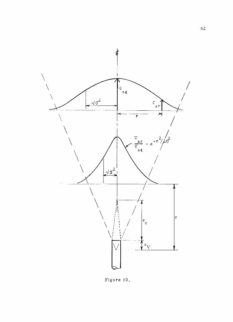
the profiles based on turbulence theories They wrote

v 2 2 zr -r 2CY Il-l 2 5 =ev ztshy

2where CY is the variance of the distribution as depicted in Figure

10 (Henceforth the overbar designating the average value will be

dropped)

52

I- v

zt

I 2(J ----~- -----~~-middot

r

I - 22 zr o e-r ~U

z

2

fJ I

I

II I

I I I I I o

zI I I

I z

c I I I

I I

v zv

Figure 10

53

The constancy of momentum flux plus the assumption of similarity of

velocity profiles gives for this profile

2~(J

= c z

a constant which must be empirically determined The constant when

evaluated also serves to express the decay of center line velocity

with distance from the end of the core region z iec

v D z ~ = __2_ c

Il-l 26 v 2cz z

J

where v 1s the velocity in the jet and D is the jet diameter J J

Combining these expressions

v 2 2 2 zr = e- r 12c z II-127

v zt

or

v D 2 2 2 zr 2= __l_e -r c z Il-l 28 V 2cz

J

They also showed that

Il-l 290 D

J J

54

which seems to invite

4cz0 0 =--~ = TICVDz II-130

z D J JJ

The value of c was found to be 0 081 for experiments in which proshy

files were measured at sections out to 64 diameters and velocities out

to 300 diameters Reynold 1 s Number varied from 1500 to about 6000

(by my calculation) and was assumed not to be a factor in this range

Baines (1950) in his discussion of the paper above reported his studshy

ies where Reynolds Number NR was varied from about 8500 to

aver 100 000 to show that as NR increased (especially above

20 000) the value of c decreased (My estimate of his data would

show c = 0 095 NR = 20000 and c =0 081 NR = 130000)

Hinze and Van de r Hegge Zijnen (1949) studied heat mass and

momentum transfer in an axially symmetric air jet mostly at an

4 NR of 6 7xl 0 however a few tests were also run at N 1 s from

R 4 4

2xl0 to 8 4xl0 to convince them there was no effect on the shape

of the profile in this range Heat transfer was produced by using a

slightly heated jet usually about 30degC above ambient Addition of

1 1oo of 11 town gas 11 allowed them to follow mass transfer by means of

a sensitive gas analyzer In comparing their experimental results

with the various theories they felt as did Corrsin (1943) that the theshy

aries should be checked only in the fully turbulent central region near

55

1 the axis Corrsin felt that the region out to v = -v would be

Z 2 Zi acceptable however Hinze and Zijnen used oscillographic data to

show that this region increased in diameter as NR increased and

for most of their tests the cornparison should be made out to

v =0 3v In any event they matched curves at the 5 point and Z Z

found heat and mass to disperse equally but somewhat faster than moshy

rnentum They were able to show that eT was nearly constant

across any section (Prandtls second hypothesis) but that EH was

not The ratio eTeH (the trubulent Prandtl ) or eTem (the turshy

bulent Schmidt ) varied from 0 7 on the ct_ to 1 3 at r z =0 14

For average values to be used for practical purposes they calculated

E 2__1 _ 0 1 24m s e c = o 73- 2 EH 0170m sec

The authors felt that the difference in density ( 6-7) caused by

the heated air did not influence the results an assumption which is

now known to be erroneous

Forstall and Shapiro (1950) investigated mass and momentum

transfer from a turbulent axisymmetric jet to a co-flowing annulus of

the same fluid at the same temperature Here also mass was found

to transfer more rapidly than velocity and the turbulent Schmidt Numshy

ber was found to be about 0 7

Forstall and Gaylord then studied the problem of a jet in water

56

to test Albertson et als (1950) solution and to obtain information on

the turbulent Schmidt Number for water which can be ex-

E

pressed as

R 2 v

N =(-) II-131S R

e m

when the transverse profile is expressed as the error integral The

tank employed was over 100 diameters deep but no profiles were takshy

en above 30 diarneters Although the data seem to be in good agreeshy

ment with the data of Hinze and Zijnin (1949) and with Albertson et al

(1950) and in fair agreement with Corrsin and Uberoi (1949) the comshy

puted values of N seemed to be systematically high a condition 5

E

for which the authors expressed concern but which they could not exshy

plain It may be that the method employed of determining mass transshy

fer was the cause The jet consisted of fresh water while the tank

contained 1 by weight of sodium chloride so that samples obtained

from the mixing region could be analyzed for salinity The initial jet

velocity was not given but if it were relatively small the densimetshy

ric Froude Number N defined asF

4v

N = --======shyF gDtpp

J 1 s

4 hPs 1s t e density of surrounding fluid and tp is the initial difshyference in density

1

57

might have been low enough to indicate a considerable buoyancy force

contributing to diffusion This will be discussed further later

Horn and Thring (1955) investigating the trajectory of a flame

jet in a furnace assumed different error functions for the velocity and

concentration profiles and constructed an empirical formula for the

trajectory which was good between 12 and 120 diameters downstream

For the case reported the jet density was twice that of the surroundshy

ings Later (Horn and Thring 1956) they investigated the effect of

p I

p s on the angle of spread of the jet a They found a = 17deg

for pp varying from 1 to 2 and showed results of two tests J s

However their experimental device employed a jet entering a slowshy

ly moving mass of fluid and no further information regarding thereshy

lationship of the two velocity vectors is given Abramovich (1963)

p 229-232) covered this topic extensively and showed that a coflowshy

ing stream (within certain ranges) substantially reduces the angle of

spread

Using apparently the same apparatus Bosanquet Horn and

Thring (1961) reported the co flowing velocity as 0 04 ft sec which

when compared to their smallest jet velocity of rv 9ftsec was sureshy

ly negligible and could not have affected a They went on to show

that the axis of symmetry in the deflected jet (as judged from the outshy

line of a dye field) was also the axis of the concentration profile howshy

ever in so doing they showed a profile which is very unusual They

58

developed a formula for predicting the centerline or axis of the jet

using empirical constants evaluated from Hinze and Zijnen (1949) and

by assuming the profile was represented by the error integral The

calculated formula checked very closely with many experimental runs

Either the formula was insensitive to the form of profile assumed or

the profile shown was not representative

Keagy and Weller (1949) investigated velocity and concentration

profiles for jets of nitrogen heliun1 and carbon dioxide issuing at

400ftsec through a Ol28diameter orifice into still air Taking

into account the diffe renee of density (due to molecular weight) but

neglecting compressibility they found good agreement with the formushy

las

- shyv v = e

2 2 -br jz

II-132 Z Zf

2 2 = e -abr z II-133

where w is concentration

The constants for the various gases were found to be

For Nitrogen Hydrogen Carbon Dioxide

b = 88 57 101

and a= 72 50 85

Hence in all cases matter diffused more rapidly than did momentum

but the rate seemed to be markedly dependent on density They also

reported that momentum and concentration were only approximately

59

conserved as determined by the profiles the percentage conserved

falling off as zD increased J

Voorheis and Howe (1939) earlier had reported the same probshy

lem - after 40 diameters downstream errors of 15oo were observed

for air rnomentum and 25oo for gas momentum The results for veshy

locity and concentration profiles showed typical results in general

but there were some unexplained discrepancies

About the time the theory was developing Rawn and Palmer

( 19 30) were working on a very extensive application of jet diffusion shy

disposal of Los Angeles sewage into the ocean - and unaware of the

theoretical developments they undertook an experimental study to

develop empirical guidelines for design use They found that the

amount of entrainment was related exponentially to the axial distance

to the surface and that the diameter of the mixing region was approxshy

imately equal to zc These are facts which we now know to be in

accord with the theory developed The thickness of the diluted sewshy

age field spreading horizontally at the surface was found to average

z 12 and because the velocity was continuously dec reasing the max

rate of dilution was decreasing although for the samples they took

the increased dilution with distance was measurable They found the

time required for the layer to travel given radial distances at the surshy

face r was 11 exceedingly 11 uniform and expressible as zmax

60

32rrr z Df zmax max max _Jt = II-134+ 249QS 8

J zmax

where Q is the volume flux in the original jet and s is J zrnax

the dilution (a function of z c) They calculated that if the surshymax

face of the ocean were slightly warmed and the dilution was under a

critical value the layer would be thinner and hence spread more

rapidly

Rawn Bowerman and Brooks (1960) reconsidered the results

of the 1930 study and decided that the empirical equation for S was

restricted because of the possible lack of similitude incorporated in

the study which they then sought to rectify Phenomenologically

they knew that in a simplified case S could be considered a zmax

g 6pmiddotfunction of z D v __1 and v These six variables are max J J ps J

represented in four independent dimensionless nun1bers S zmax

z D NF NR of which NR was considered of little influshymax J

ence in the fully turbulent region above NR = 5 000 and is neglectshy

ed by restriciting consideration to that region hence

S = f(z D N ) II-135 zmax max J F

Using the 388 observations of Rawn and Palmer (1930) smooth

curves for various S were fitted to values of z D and zmax max J

61

NF some of which are approximately reporduced below in Figure

11

z max

120

100

80

50

D 30 J

20

10

___----Increased outlets

(~ COrtstant J

30

l

~ h ( )

I

I

s zmax

2 3 4 5 10 20 30 40 Nl

F Figure 11

In any situation dilution can be enhanced by setting the diffuser

deeper For any given setting and outlet diameter an increase in v J

represents moving on a horizontal line on the graph and the value of

thif move is seen to depend on the original setting Keeping Q J

constant but reducing D causes an increase in zD as well as J J

The re suiting slope is 0 4 which is seen to always reshy

sult in increased s Providing a larger number of smaller zmax

62

outlets so that v and Q remain constant increases dilution at J J

a rate of 2 bull a solution which the authors felt is the most approprishy

ate In discussing the complicating effects of thermal stratification

on this analysis the authors stated (p 88)

When the sewage field does not stay at the surface the temperature ampradients are still beneficial in making the sewage field thicker and hence more dishylute Since the edges of the rising jet become dilutshyed most rapidly this PriphmiddotbullHal flow is stopped at a lower level even though the l~ss dilute central core breaks through to the surface

Abraham (1960) extrapolated the reasoning of Rawn BowermaI

and Brooks to include the dimensionless radial distance rD as J

an independent variable in computing vv and w w hence J J

6pv z r 1

N) ll-136 v =fl( Dmiddot p D F

J J J J

and

6 pw z r 1- N) II-13 7=f2 ( Dw D p F

J J J J

The problem is divided into three parts 1) non-buoyancy case

(N = oo) whereF

v c D b 2 2z 1 1 - r z = ~ e II-138

v z J

63

and

w = c D 2 2 ~_1_ e -abr z

II-139 w z

J

The results of five other investigators were evaluated in the above

form to present values for a b c and c as follows 1 2

a b cl c2

76 6 2 08 77 64 5 2 ~elected 0 71 88 5 8 59 074 100 0 70 96 6 6 54

from which he selected the indicated values since they were obtained

from experiments by Forstall and Gaylord (1955) on water rather

than on gas The constant b was reported not to be influenced by

p p in the range of our concern s J

(2) buoyancy only case (NF =0) Here Abraham found theashy

retical and experimental evidence for

v 2 2 z _ 65NF-23lt + 2)-l3e -80r z= 3 II-140

V J J

and

2 2 w

7N 23(~ 2)-53 -80r z= 9 II-141 w F D+ e

J J

which were based on the assumptions that (a) the velocity and buoyant

64

force (g 6p) profiles (and similarly the concentration profile) are

the same at any section and similar at all sections (b)

a(Q-Q)J

f(v ) and (c) p gt gt 6p az z s l

Abraham 1 s statement that the solution requires the assumption that

the velocity and force are constant across the jet is in error (Morton

Taylor and Turner 19 56) as this is clearly incompatible with the

above equations What Morton et al merely said was that assumpshy

tions a and b above allow use of the principles of conservation of

momentum volume and density deficiency (or heat or concentration)

fluxes and as an illustration of this principle the profile could be

averaged in some way to satisfy the momentum equation over some

section This is demonstrated in Figure 12 where the momentum

flux of the 11 averaged 11 profiles equals that of the actual profiles

Note also that the profiles he assumed do not agree with those in

case (1 )

-(--shy

Actual

Averaged profiles

Figure 12

65

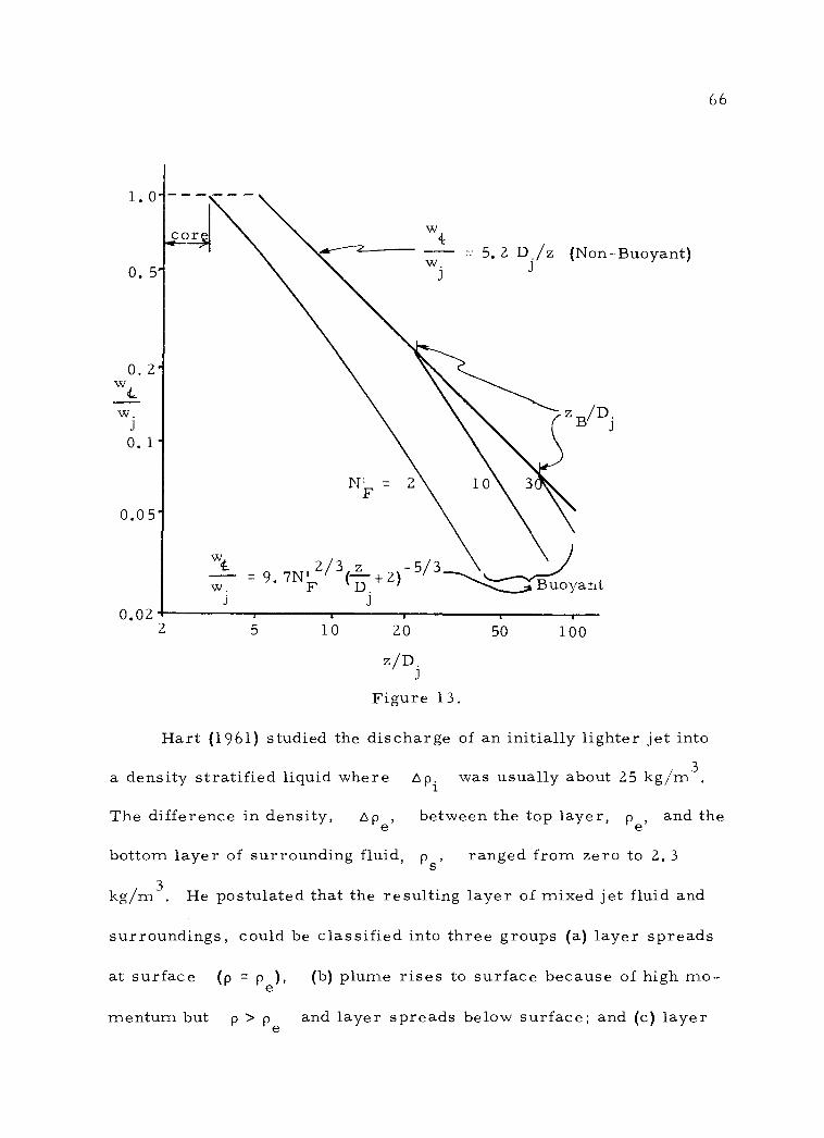
(3) Intermediate case (NF finite) The theoretically derived

equation of Schmidt ( 19 57) suggested to Abraham that the initial proshy

tion of the mixing region could be described as the non buoyant case

and the final portion as a buoyant situation The transition occurs at

z where for sufficiently large values of z and N 1 bullFB B

2 zgN 1 B oo

- 6 92 II-142[ S dz S (ps -p)rdr2 pv D 0 0

J J J

When NF is greater than about 10 zB can be approximated by

1z D - 2 43NF II-143 B J

Abraham analyzed the salt concentration in samples obtained along the

axis of a fresh water jet discharging into a small tank of salt water

3(density= 1020 to 1050 kgm ) to verify these equations The final

form is demonstrated in Figure 13

66

o 5

w J o 1

oo 5

002

cor

wt

w J

lT = F

w J

= 52 Dz (Non-Buoyant) J

= N 23 2_ 2 -53 ~ 9 F ltD+ ) ~Buoya-1t

J

5 10 20 50 1002

zDJ

Figure 13

Hart (1961) studied the discharge of an initially lighter jet into

3 a density stratified liquid where 6p was usually about 25 kgm

1

The difference in density between the top layer and the6 p e

bottom layer of surrounding fluid ranged from zero to 2 3ps

3kgm He postulated that the resulting layer of mixed jet fluid and

surroundings could be classified into three groups (a) layer spreads

at surface (p = pe) (b) plume rises to surface because of high moshy

mentum but p gt p and layer spreads below surface and (c) layer e

67

spreads at thermocline without touching surface He determined

the height over the discharge point at which the layer is established

as a function of a buoyant force parameter B and NF (NF

defined according to Abraham) viz

II-144

In attempting to evaluate the nature of the function experimentalshy

ly there appeared to be a good deal of overlap in the latter cases (ie

b and c) and it was necessary for him to redefine the resulting fields

as (A) surface (B) continuing thickness with time (to limits of equipshy

ment) between surface and thermocline and (C) submerged at thermoshy

cline He found that if he expressed B in terms of the density in

the mixing region which was in turn affected by NF then he c auld

predict the group fairly well but not zL A value for B based on

p at (height to the thermocline) according to Abraham was

not as good as his own method of using p which depends also ZTC

on Abrahams solution viz

Pz -pe

10 4( T[CB = ) II-145 p

J

where

p = p -05lw II-146zTC 6piZTC s

68

and where 2

= N 23( TC 2)-539 II-14 7wf zT jc wj middot F D + J

is the concentration evaluated at the height of the thermocline and on

the centerline His results indicated that for

B ~ 0 Group A resulted

Group B resulted

B8 Group C resulted

For Group C the height to the center of the layer was found to

be

zL 95z_ =98+--_P II-148

D D J J

where z_ is the distance above the discharge to the point on the p

original density vs depth curve where p = p Only a very2 TC

poor fit could be found for the best empirical formula relating condishy

tions to the final field thickness h viz

h ze D =77+023D II-149

J J

where

z = z f - zT =thickness of epilimnione sur C

In discussing Harts paper Abraham (1962) reported a theoretical

69

solution to the problem although he does not present the derivation

His result gave the highest level z reached by the mixed max

fluid as

z 3 1 2 3 2

ltmaxgt = (o4BIFI+o9)(032IFI+o6) + (o32IFI+o6) II-150 ZTC

2where v

F = ___4_middot ZTC II-151

p - p e tf zTC

( p )gzTC J

Note that here the Froude 11 number F is considerably different

than that employed previously On form it is the square of N theF

velocity is the velocity on the ltf of the mixing region where z is

the distance to the thermocline and this distance rather than D is J

used as the characteristic length The choice of p rather than p s J

or as the denominator of the density factor is consistent with

his previous definition According to this solution if

p -p gt 0 then Group A e t zT C

z -z max TC gt 1 then Group B

z e

z -z max TC-------- lt 1 then Group C

z e

The results of employing these criteria to Harts data are summarized

70

as follows

Hart Abraham zmax- zT(_C

B Group Group pe- Pt zTC z e

-5 -4 -4 -4 - 3 -2 -2 -0

4 5 7 7 7

8 13 14 16 17 17 17 19

~~22

A A A A A A A A A A A A A A A A

B A B A B B B B c B c c c ~ I B c B c =c c c c c c c c c c c

1 03 79 75 71 56 47 33 77

03 04

negligible negligible negligible negligible negligible negligible negligible negligible negligible negligible negligible negligible

4 15 1 34 1 01

77 1 37 1 45

56 76 70 57

44

28

The most serious discrepancy seems to be in the region indicated by

the arrow brackets ( r ) Hart pointed out however that the starshy

red results were for NR = 1700 while all the other runs were at

NR gt 3100 If these two results are neglected then it is only a matshy

ter of a shift which separates the two methods

Abraham (1963) subsequently published his theoretical solution

71

which included an elaborate treatment of flow in the core region (afshy

ter Albertson et al 1950) and a general solution for forced plumes

inclined at any angle with the horizontal discharging into a uniform

ambient environment He presented a graphical solution (based on

Priestley and Ball (1955)) for vertical upward discharge into a unishy

formly stratified fluid and an incremental method for vertical upward

discharge into an environment with arbitrary non-linear gradient He

employed the boundary layer approximations and assumed both unishy

formity of pressure and similarity of profiles (Gaussian outside of r

core) This allowed the approximation 0 =c although he show-

z

ed this not to be true if both buoyancy and initial momentum exert an

influence at any point in the mixing region For solution of the probshy

lem when buoyancy is negative he suggested entrainment is negative

which is taken to mean that the volume flux in the positive axial direcshy

tion is decreasing due to horizontal spreading because at the same

time he states 11 bullbullbull near the ceiling level the concentration of the polshy

lutant remains constant at the axis This assumption was employshy

ed to provide the solution

The above problems were divided into three categories

A N-- oo (non buoyancy)F

B N 1 _ 0 (buoyancy)F

c N =finite (intermediate)F

72

and each forced plume was considered to possess two zones

a flow establishment (core)

b established flow (mixing region where similarity prinshy

ciple is applied)

At this point he misinterpreted Mortons (19 59 b) treatment of virtual

source location as an attempt to include consideration of a core

whereas Mortons reasons were based on the necessity of zero mass

flux from a point source and that the similarity hypothesis was apshy

plied throughout the distance traveled by fluid particles He also used

his assumption of r z =c to prove that Taylors assumption of 0

constant entrainment (used by Morton) is erroneous However he

did not point out that Mortons solution does not require this assumpshy

tion

To be sure Mortons solution provides this result only for the

case of uniform ambient environment but for the case of a stratified

environment the solution provides a non-linear increase in r 0

with zmiddot a result which is in accord with the observed phenomenon

Abrahams solution is based on the empiricism that a mixing length

exists which is constant throughout the cross section and proportional

to the plume width clearly no better than Taylors empiricism Ab-

rahams solution for v and w in the zone of established flow z

with finite N is essentially the same as those of Priestley andF

Ball (1955) and F H Schmidt (1957) He found

73

v D bK 312 3(1 )b 2 z 2

I21_ =__1[(-c) + +a (~ __c_)] l 3 Il-l 52 V z 2Kj 8NF 2a D D 2J

J J

and

b(lta)D bK 312 2 z 2 I

~ = [( c) + 3(lta)b (~ __c_)] -1 3 Il-l 53 w 4z 2K 2 D 2

8N a DJ J F J j

In the above results z and K are different for velocity and concenshyc c

tration and for various Procedures for finding z and K c c

were given For large z 5D (ie NFgt6) while forN

c J

N I - l 4 z bull 2D 0

F c J

Morton assumed a and b are independent of N but the F

experiments of Corrsin and Uberoi (1949) showed that b increases

with 6 p hence with liNF

middot and those of Baines (1950) showed

that b increases with NR On the other hand the work of Hinze

and Zijnen (1949) showed no measurable difference over an admittedshy

ly smaller range of NR and Horn and Thring (1956) showed no

change in the angle of spread for a large reange of 6p Abraham

employed the energy equations to show

bN oo 2 4aN = 0 _ ______ l( F ) = F - Il-l 54

b ltaNN = 0 F=OF

74

3(1-a)z 2

I 2b 2 4aNFPN =00 J

F----middotmiddot) = 1 Il-l 552b

zl z K 32 cb I (-c) + --)2K DzJ

J

The fcllowing figure Figure 13 represents this variat10n of b by

showing the effect of N on the relative p1nn1e width (DDF

I

NF

for various values of zD The vanation is not excessive at a l

_D___downstream distance of 30 diametels I JJ

=0918forN=F

N = ~ F

and 0 987 for NF= 35

1 00

098

09b

J )4

01)2

D

=CO

2 4

N F

7 1 5 30 ~00

z D J

Figure 13

He subsequently employed

N = oo b = 77 a = 0 80 F

N~= 0 b=92a=074

designing the physical model studies incorporated in this study

Experimental values of maximum penetration and of the posishy

tion of the horizontally-spreading layer were obtained in a one meter

deep tank of 2 4 meters diameter Stratification was obtained with

salt solutions of varying densities The results from runs using five

different gradients and the results of analyzing the experiments of

others demonstrated that the method is suitable for obtaining a rough

approximation of the location of the bottom of the horizontal layer

Its use for estimating maximum penetration is discounted on both

theoretical grounds and experimental evidence Both levels were unshy

derestimated by the mathematical model in comparison to the exshy

perimental values

A computer program was employed to solve the equations and

rounding errors as well as inefficient methods of quadrature were

found to account for as much as forty percent of the discrepancy beshy

tween observed and predicted values

Vertical Jet Diffusion in Non Linear Density Stratified Fluid

by

Donald John Baumgartner

A THESIS

submitted to

Oregon State University

in partial fulfillment of the requirements for the

degree of

Doctor of Philosophy

June 1967

APPROVED

Professor of Civil Engineering

Dean of Graduate School

Date thesis is presented May 11 1967 ----------~--~--~~-----------------

Typed by C 1 o ve r R e dfe r n f o r ____DonaldJohnBau=mg2artn-=-=e-=r--shy

ACKNOWLEDGEMENT

The writer is indebted to the Federal Water Pollution Control

Administration and to Dr Leon W Weinberger of that organization

for complete financial support for the program of research reported

herein

Appreciation is expressed for the guidance and support receiveJ

from Dr D C Phillips Professor F J Burgess and Dr L S

Slotta of the Department of Civil Engineering and for the financial

support for computer services received from Dr D D Aufenkamp

Director of the Computer Center Oregon State University Helpful

suggestions and encouragement were received from Leale E Streebin

during the course of this study and should be acknowledged Thanks

are also due to Mrs Maureen Gruchalla for her patience in typing

the first draft of the manuscript

Finally the dedication perseverance confidence and enshy

couragement of the authors wife Therese and their children were

essential to the successful completion of this program and are grateshy

fully and sincerely appreciated

TABLE OF CONTENTS

Page

I INTRODUCTION 1 Mixing of Stratified Reservoirs 1 Improving the Design 3 The Problem to be Solved 4 Fundamentals and Definitions 5

II PREVIOUS INVESTIGATIONS 7

Flow Into Density Stratified Fluid (Linear

Initial Independent Variation of Buoyancy

Development of the Theory 7 Lanltina r Jet 7 Turbulent Jet (No Buoyancy) 9 Turbulent Plume (No Momentum) 21

Gradient) 24

and Momentum 27 Extension of Thea ry 48

III PROPOSED IMPROVEMENT 85 Normalization 85

Stratified Environment 85 Uniform Environment 96

Solution of Equations 99 Stratified Environment 99 Uniform Environment 114 Solution of Problem 115

IV MODEL STUDIES 118 Similitude 118 Experiments 120

Mathematical Arrangement 120 Physical Arrangement 121

V RESULTS AND ANALYSIS OF DATA 130

VI DISCUSSION OF RESULTS 136

VII CONCLUSIONS 145

BIBLIOGRAPHY 147

APPENDIX Appendix I Appendix II Appendix III Appendix IV Appendix V

Page

157 157 159 160 162 167

LIST OF TABLES

Table Page I Hydraulic characteristics of experimental runs 126

II Comparison of predicted results for Run Two 133

Ill Comparison of experimental results with predicted

values for zmax and zLBOT 133

IV Observes and predicted values of Hart 1 s experiments 140

VERTICAL JET DIFFUSION IN NON LINEAR DENSITY STRATIFIED FLUID

I INTRODUCTION

Jet diffusion is involved in at least three currently important

problems confronting sanitary engineers (1) dispersion of liquid

wastes from outfall sewers (2) dispersion of stack gases into the atshy

mosphere and (3) mixing of density stratified impoundments The

first two are well known and their relationships to the theoretical

study of jet diffusion has long been established The third problem

has many interesting facets only a portion of which can be investigatshy

ed via the same theory Because this is a relatively new application

additional background information may prove valuable

Mixing of Stratified Reservoirs

Frequently storage capacity is included in multi-purpose reshy

servoirs for downstream water quality control but unfortunately

this storage in itself may impair quality To combat this mechanical

mixing has been employed and is currently considered among the passhy

sible methods of quality control For a general discussion of this

problem the reader is referred to Symons Weibel and Robeck (1964)

Mechanical mixing has also been used to prevent or remove ice forshy

mations from reservoir surfaces and these applications provide the

2

bulk of the technical documents available on the subject

The physical nature of a reservoir which causes the problem to

develop is related primarily to the density-temperature function of

water which allows a body of water to become density stratified under

the influence of solar energy and wind induced surface currents

Hutchinson (1957) gives a good presentation of the physics of stratifishy

cation and the types of density-depth profiles which have been found

They are customarily non-linear Of secondary importance at least

in fresh water impoundments is the density gradient induced by the

varying concentratwn of dis solved salts

Returning to the cases where m1xing has been employed eight

tests have been reviewed in which diffused air was employed at rates

ranging from 0 03 to 3 cubic feet per minute per acre foot (cfmAF)

of volume One test (Patriarche 1961) in which the aeration rate

was between 0 06 and 0 08 cfmAF was unsuccessful while the others

were considered successful Although the data are incomplete it apshy

peared that the higher rates were associated with shorter operating

times hence the energy inputs per unit volume were not as widely

separated as the rates Several attempts at mixing have also been

made using pumps to transfer cold water from the hypolimnion to the

warm epilimnion where when discharged from a pipe mixing occurs

by jet diffusion However sufficient data for comparison of energy

requirements are not available The point to be made is that these

3

devices are be1ng used and considered for additional use in spite of

the fact that nowhere has a rational or fundamental basis for such a

design been set forth

Improving the Design

It seems only reasonable that the size of the reservoir the deshy

gree of stratification the power of the device and the time it 1s to

operate are involved in the design

The items of power and time have two limits imposed on them shy

an economic and a natural limit If it turns out that an energy expendshy

iture of X horsepower-hours (Hp-hrs) is required to reduce the

stratification a certain amount this can be achieved with any set of

values for power and time such that their product equals X Howshy

ever a massive pump which would operate for a short time would not

necessarily be the most economical arrangement since its first cost

would be extremely high and its unit operating cost would be low On

the other extreme it is realized that the natural forces causing stratshy

ification operate on a cycle somewhat less than annual and hence any

small pump requiring an ope rating time greater than this is naturally

unacceptable

Many choices are available to the engineer and to narrow down

the discussion only vertically oriented devices will be considered

further even though devices discharging horizontally are occasionally

4

used in this practice

Whether discharging from a line source or a point source when

a vertical device is used the degree to which stratification is changed

by mixing can be related to the volurne flux and the location of the

horizontally spreading mixed layer In addition to location the vela-

city of the spreading layer is important since high velocities encourshy

age additional entrainment by vertical mixing across the density

boundary Abraham (1963) provided additional comments on this

These parameters can be related to conditions at the terminashy

tion of a zone of vertical jet diffusion A rational basis of pump or

aerator selection will be provided if the required terminal condishy

tions can be related to the physical source variables and the density

gradient in the fluid For a single point source these variables would

be the jet or orifice diameter D the velocity of discharge vJ J

the initial density difference between the jet fluid and the receiving

fluid 6p l

The Problem to be Solved

Before approaching the problem of optimizing the selection of

input devices it is first necessary to be able to relate the input varshy

iable s to conditions at the onset of the horizontally spreading layer

At present as the literature review will show these relationships

are not available By assuming a completely quiescent ambient fluid

5

the problem is greatly simplified Abraham (1963) has given an apshy

proximate solution to the basic portion of this problem but the speshy

cifically desired answers are not readily available This study will

be an attempt to solve specifically for

1 The maximum height reached by a forced plume

2 the initial volume flux in the horizontally spreading mixed

layer

3 the location of the horizontally spreading mixed layer

The solution is to be sought for the case of a single circular source

Fundamentals and Definitions

In elementary fluid mechanics practical solutions to problems

are frequently found by idealizing the flow to neglect friction Detershy

mining the trajectory of a jet of water in air and the coefficient of

contraction for flow from a Borda mouthpiece are examples of fruitshy

ful utilization of ideal flow approximations Unfortunately when a

liquid jet is discharged into a liquid this simplification can no longer

be accepted due to the important action of viscous friction Preservshy

ing the simplifications of steady incompressible flow with no velocity

fluctuations (laminar) fluid motion can be described by means of the

Navier- Stokes equations The net force of gravity is cancelled when

both liquids are of the same density and by specifying additionally

that no angular component of velocity exists (two dimensional

6

axisymmetric) the equations of motion are written as

2 2 v ov v ov a v ov v a v

r r z r aP r 1 r r r + = + v(-- +--- -- +--) I-1or oz p or 2 2 ~ 2or r or r uz

2 2 v OV v ov ~ a v av a v

r z z z uP z 1 z z + =--tv(--+--+--) I-2or oz ar 2 az 2 paz r or

The equation of continuity for these specifications is

ov v ov r r z+-+--=0 I- 3or r az

The symbol v represents the kinematic viscosity P the presshy

sure and the other symbols are defined in Figure l

v z

With this fundamental theoretical

background early investigators

attempted to develop a theory to

describe the nature of jet diffushy

sian

Figure 1

7

II PREVIOUS INVESTIGATIONS

Development of the Theory

Laminar Jet

When a fluid is discharged through a circular orifice into an inshy

finitely large expanse of similar fluid at rest fluid is entrained from

z the s tationa ry fluid due to visshy

cous forces The downstream

velocity is decreased as more

and more fluid partakes in the

flow Although the affected area

ideally extends to r = plusmnoo for

some arbitrarily small value of

v the horizontal distance z

r at which v is obtained 0 z

describes a line (on an axial

plane) whose equation is

nFigure 2 r = Y]Z bull In 1 9 3 3 Schlichting

0

(1960) gave an exact solution for this type of problem by assuming

(1) that the pressure in the main direction of flow was nearly conshy

stant (2) the velocity in the r direction was everywhere small

compared to that in the z direction (3) that the spatial rate of

r

8

change of v is much greater in the radial than in the longitudinalz

direction The latter two assumptions are the essence of the boundshy

ary layer approximations which had been recently advanced to solve

flow problems involving solid boundaries (Schlichting 1960 page 109)

Their use in free boundary flows as in jet diffusion and wakes was

only now emerging By comparing the order of magnitude of the terms

involved in Equation I-2 (Schlichting 1960 page 182) he showed that

o2 v oz 2

could be neglected giving z

ov ov ~ ov z z 1 u z v -- + v = v--(r-) II-1

z oz r or r or or

Similarly he showed that all the terms of I-1 were insignificant comshy

pared to II-1 and could be neglected entirely The key to the solution

was in the next assumption that the velocity profile was of constant

form at all sections It is this assumption which characterizes a

group known as similarity solutions Knowing or assuming the

flow at some section say the orifice provided the boundary condishy

tion of K the kinematic momentum flux

2 K = 2rr f v z rdr II-2

0

which is constant

9

The solution was given in terms of the parameter ~ where

t - ~[Ks - II-3 vz 161T

3K 1 as v = II-4

z 81TVZ(lt __ ~2)2 4

and v = II- 5

r

Fur thermo re 0 the volume flux was found to be

0 = 81TVZ II-6

which is seen to be independent of the inlet flux 0 J

Andrade (1937) tested Schlichting 1s solution in a smalllaborashy

tory apparatus and found good results between Reynolds number=55

to 300 For Reynolds number (NR) gt 180 the velocity distribution

at the orifice could be assumed uniform in order to compute K

Turbulent Jet (No Buoyancy)

The study of turbulent jets which are free from boundary efshy

fects was enhanced because turbulent friction is so much greater than

laminar friction in the main flow that laminar friction may be negshy

lected FUrthermore because there are no walls it was not necesshy

sary to consider the laminar sublayer which ordinarily could not be

10

neglected Since the observed nature of turbulent jet dispersion exshy

hibited similar characteristics to the laminar jet namely (a) the exshy

tent of lateral flow involvement was small compared to the longitudishy

nal extent and (b) the lateral gradients of velocity were much greater

than those in the main direction of flow the use of Prandtl s boundshy

ary layer approximations again allowed a 2 v oz 2

to be neglected z

as well as the equation for the r direction Consequently the

equations of motion were written in identical form as for the laminar

case ie

2a--v av a v av z z z 1 z

v +v = E (-- +--) II-7 z oz r or T or r or

where the overbar designates the time average In solving this equashy

tion simultaneously with the continuity equation (Equation l-3) which

remains unchanged it was necessary to ernploy assumtions regardshy

ing based on empirical evidence Prandtl s mixing length thea-ET

ry was successfully employed for this purpose (Schlichting 1960 p

591) Although normally expressed as

Il-8

Prandtl also hypothesized a relationship for free stream turbulence

(as a jet) which expressed ET as proportional to the width of the

mixing zone and velocity fluctuations in the transverse direction ie

ll

= cr v II-9 o r

where the prime designates the fluctuating component Additional

evidence extended this to include the dependence of v on r

hence

= c r v Il-l 0 1 o zltt

He used the similarity assumption with n = 1 hence

r 0

and thus

= c zv 3 zltt II-11

For the laminar jet and supported by empirical evidence of turbulent

jets

then

II-12

a constant

Employing ET as a constant the situation was entirely analoshy

gous to the laminar case where v was a constant and the results

were (the time average quantities designated above by the overbar

as v are henceforth represented without the overbar) z

12

v z

3 (~-1 )

4 v =--0_2_2_ f[f

r

z(l + )

~ __r_ ~ -e zJ~ T

Q = 8Tie z T

The constant e must be determined empiricallyT

(1960 p 608)used E =00161-KT

hence

7 41-JK v =

z ~ 2 2 z(l +4 )

3 v = 0 244fK (~-5_ )

r ~ 2 2 4 z(l +4 )

r ~ = 15 2shy

z

Q = 0 405-JKz

II-13

II-14

II-15

II-16

Schlichting

II-1 7

II-18

II-19

II-20

Possessing a knowledge of the velocity field and the volume

13

flux is not however the ultimate goal since the final temperature

(or density) of the water from the jet is de sired Applying Prandtl1 s

hypothesis of momentum transfer to the case of heat transfer would

imply that the temperature distribution would be the same as the veshy

locity distribution ie

dv z dT

T = pe -shy and q = c pe - II-2122T dz p H dz

dv dv dv2 z z 2 z dT

T = ppound ~~~~ and q = c ppound 1-1- II- 23 24 p dz dz

While such a situation is frequently observed in flows influenced by

walls it is not found in free turbulence here the temperature disshy

tribution is spread out as shown schematically below

v distribution

Figure 3

By way of symptomatic adjustment the profil~s are accounted for if

- 2e or in terrns of the mixing lengths 7 pound T T

14

There is however a theoretical justification for this result based

on Taylors (1915) vorticity transfer theory which assumes that a

two dimensional eddy conserves its vorticity The theory predicts

the sarne value of eddy viscosity as Prandtls theory and hence leads

an 1d t ve 1oc1ty d butlon- l T 1 (1932) d escr1 h1sto en 1ca1 1str1 ay or bes t

theory and its differences from Prandtls momentum transfer theory

in a very straightforward n1anner and then shows that for heat transshy

fer his theory predicts a temperature distribution (adjusted for coinshy

cidence of maximums) which is the square root of the velocity distrishy

bution or that EH = 2E T The experin1ental studies of Fage and Falshy

kner (1932) and according to Schlichting (1960) those of Reichardt

(1942-not seen 1944) show good agreement for this result The disshy

tribution equations are not given here since they pertain to plane (two

dimensional) flow

The extension of the vorticity transport theory seemed a naturshy

a1 step but as Taylor (1935) pointed out the resulting equations are

useless due to their complication unless simplifying assumptions

are made A special type of 3 dimensional flow - that exhibiting symshy

metry around an axis - reduces the equations to a type containing two

This is actually a special case of two dimensional flow and the only one where the results would be similar Here the turbulence in the direction of flow can be neglected and turbulence can be considshyered to be restricted to the coordinate transverse to the direction of flow In other two dimensional cases where the longitudinal turbushylence cannot be neglected the results are different

1

15

coordinates and is one such assumption Taylor then assumed that

the nature of the turbulence is such that the components of vorticity

are transferred without change to a new position and the eddy retains

these components until mixing occurs with the surroundings The use

of this assumption constitutes the modified vorticity transport theshy

ory

Goldstein (1935) simplified the general theory for axisymmetric

flows by assuming in addition that the turbulence was symmetric

about the same axis

Goldstein (l938a) compared results on velocity profiles obtainshy

ed by Schlichting and Prandtl in the wake of axisymmetric bodies in

order to evaluate these various theories Incidentally it should be

noted that judging from Schlichtings (1960) work the distribution

functions in the wake of an axisymmetric body are similar to the disshy

tribution functions in an axisymmetric jet in a medium of equal denshy

sity He found a poor fit to their data with the momentum transfer

theory Equation II-25 which is plotted as curve 1 in Figure 4

v 32 2 z

=[l-0293(~ ] II-25 v

zmax

With two solutions of the vorticity transfer theory with symshy

metrical turbulence he found a good fit only in the middle range of

data In the first (curve 2) pound was assumed to be proportional to

v

II- 26

16

1r as shown in Equation II- 26

v 4 r 52 18 r 52 1 r 152z = 1-s-ltmiddot 863R_) + 1 75( 863 R) +I 225 ( 863R) +

zmax

v z

v zmax

1 A -----shy ~

8

Curve Z

6

4

L

5 rR

] r_) z

l

Curve 4

Figure 4

ThisIn the second solution (Curve 3) was presun1ed

equation was

v 3 z z

[1-0 Z93(i) ] II- 27 v

zmax

Using the nwdified vorticity transfer theory resulted in curve 4

Equation II- 28

v z 1 4 r 3 2 14 r 3 7 r 9Z

v =3[3-31225R) +81(1225R)- 6561(1225R) - ] zmax

II-28

17

v zmax

=

r 0

v

Figure 5

From Goldsteins text of the

experimental procedure the

schematic description shown

in Figure 5 was deduced as

zrnax an aid in describing the 2

terms In regard to the temshy

perature distribution Gold-

stein had no experimentally obtained data to compare against so he

plotted the four curves and mentioned that none seemed to be satisshy

factory This result is shown later in Figure 6

Curve 1 is _T_T__ = (1-0 293(~)32]2 Il-29 max

as for v v and z zmax

TCurve 2 is II-30

T max

Curve 3 is T =1-0 293(~) 3 II- 31

T max

which is the square root of v vz zmax

18

Curve 4 is

In Equation II- 30

and

T T

max

11 1

= 0 863rR

II-32

In Equation II-32

and

11 1

= 1 2 2 5 r R

19

1

Curve 2~ 8

Curve 3T T 6 max

4 Curve 4Curve

2

r -~ 1 15 2 25 rR

Figure 6

Each of the above equations employs R which is considered proporshy

tional to r which in turn is proportional to z 0

Howarth (1938) following the work of Goldstein (19 38a) carried

out the derivation of the formulae for the most pertinent case of the

axisymmetric jet and compared it with the work of Tollmien (1945)

and of Ruden (1933) The results for the cases of axially symmetric

turbulence appear to the author as no better than Goldsteins 1 while

the cases of momentum transfer theory (Tollmien) and the vorticity

transfer theory seem to apply satisfactorily Unless Howarth had

Rudens original data not much confidence can be placed in a comshy

parison based on the graphs shown in the published work (Ruden 1933

20

since the scale is very small and no data points are plotted -merely

a curve Furthermore the equations are left in a cumbersome form

and will not be reproduced here Tomotika (1938a and 1938b) addresshy

sed himself to the same topics as Goldstein and Howarth except he

did not consider the case of symmetric turbulence which is no deshy

traction nor did he develop the temperature distribution function for

the jet For the velocity component in the direction of the jet he

iound

v z 2J 2 31 2 1 1 3 1 363J2 92 592111 6 v = 1 - 3J 3 l + 8l l 61236J3l +3582306001 -

zmax

II- 33 r

where l = --shy23

c z

The value for c was not specified but Tomotika effectively evalushy

ated it by forcing his curve through the point v jv = 0 5 l z zmax

which was specified by the experimental data Tollmien used The

equation fit the data nearly as well as Tollmien 1s equation (Tollshy

23mien found 1c = 34 edge of wake)

Kuethe (1935) investigated the velocity profile in the region

near the mouth of the jet rather than far downstream as did the other

authors As a first approximation he employed an equation similar

to Schlichting 1s and with this value for the mainstream component of

velocity substituted for v into the inertial terms of the equationz

21

of motion he solved for v in the frictional term The integrashyz

tion was constrained so that the profiles of the first and second apshy

proximations were coincident at the edge of the mixing region and at

the boundary of the core The final equations are not convenient to

reproduce here What is important was his experimental verificashy

tion - both of his work and of Tollmiens His solution very accrushy

ately predicted the velocity distribution out to about 4 4 diameters

and Tollmien s was accurate after 9 3 diameters He showed that a

central core existed whose center line velocity was maintained conshy

stant at the center line velocity in the orifice for 4 4 diameters doWilshy

stream and that the profile was changed from essentially rectangushy

lar to the typical jet profile in that distance

Turbulent Plume (No Momentum)

W Schmidt (1941) added to the more complete understanding of

the case of diffusion of an axisymmetric heated jet by considering the

case of no initial 1nomentum the motion being caused by the buoyanshy

cy associated with a heat induced density difference (The resulting

mixing region in this case is frequently called a plume) Using the

assumptions of similarity of profiles constant heat flux and a mixshy

ing length = cz he showed that

= f (I])Z -13v II- 34 z 1

22

f (ll)z -53 II-35 2

The functions of ll were given in a series expansion Rouse apshy

parently unaware that Schmidt had solved the problem also reported

(Rouse Yih Humphreys 1952) on the case of buoyancy only Howshy

ever he employed slightly different assumptions Rouse used boundshy

ary layer type approximations for the equations of motion and assumshy

ed that pgtgt6 p as well as the mixing length form of the eddy diffushy1

sian factor The result of these simplifications was that the axial

gradient of momentum flux was found to be equal to the buoyancy of a

transverse layer of unit thickness Then assuming similarity at all

transverse sections he showed that

r II- 36

cz

-l3 II-37vz ~ z

-53= g6p I( z II-38

53Q eKtz II-39

43K cz II-40

13G cltz II-41

where G is the unit buoyant force

23

II-42

where W = source output of weight deficiency or flux of incremental

weight

Note here that W is constant along the axial direction whereas

with the jet K was

He then employed dimensional analysis to establish

v z = f ( z r p W)1

and

tsy = f (z r p W)2

and then in accordance with his analytical development he set

v z r = f (-) II-43

3 z

and

ty w2 13

ltEf-gt

= r f (-)4 z

II-44

z

To fully express the functional relationship it was necessary to asshy

sume some form of profile and to fit his experimental results he

chose the Gaussian function Incidently he first showed that NR

5for turbulent mixing could be set at 10 and the height z at

E

which the plume became turbulent was

24

II-45

where W was evaluated from

W = - gqc T II-46 p

using the approximation that

6T - - II-47

T

Finally he found

v z

II-48

2 13 2 2 = _11 ( p (- W) ] e - 7 1 r z II-496 5

z

II- 50

Flow Into Density Stratified Fluid (Linear Gradient)

Batchelor (1954) in a very readable lecture Y reviewed the

problem pointing out explicitly how 6y comes to be considered as

a variable Using purely a dimensional argument with the aid of the

similarity principle he arrived at the same form as Rouse Yih and

2 Although not a part of the problem here considered it is worthshy

while to note that Batchelor mentions an unpublished work of G I Tayshy

lors asserting the identical flow regime from a line sourc~ of air bubbl~c as for a line sourc~ of heat

25

Humphreys (19 52) He cons ide red the mixing length argument of

Schmidt (1941) as an unsatisfactory approach and presumably thereshy

fore also Rouse 1 s He then extended his argun1ent to the case of a

buoyant plume in an unstable stratified surrounding fluid He claimed

similarity solutions do not exist for a stable environment a frequent

occurrence in the atmosphere

Priestley and Ball (1955) however assumed similarity of proshy

files and found the same form of solution with respect to z but

containing also aT oz They found a solution for the case where s

v and tsy could be assumed to follow the same Gaussian profile z

(requiring an experimentally evaluated constant)

For neutral conditions ie aT oz = 0 s

3 3 13D~ D v-3W J J ]v = II- 512 (l- 2 2) +z 3 3

2Tic p z 4c z 8c z

2 D 3 3 -l3-WT D v 6T = ~--s-[ -3W (l- j ) + J J ] II- 52

2 2 2 4 2 2 3 3 Tig p C Z 21TC p Z C Z 8c z

The choice of the term v 1s this writer 1 s Priestley having employshyJ

ed the value of v ie v at z = z where equals thezV z v

height above the origin (virtual source) Similarly D is employed J

rather than 2r at z = z The substitution seems to be suggestive0 v

of a more general solution where there is initial momentum

Before considering the case of thermal stratification they

26

suggested forming dimensionless quantities v and z from z

-middotshybullbull

v = v vz z zgt

= ( )13-3where 21TC p Z

hence 1-v~d l3

II-53n ] z z

From this it is seen that the fluid will accelerate upward if

gt~ 3 v lt 23 and will decelerate upwards otherwise

J

With aT az positive Priestley and Balls solution can be s

solved numerically but not analytically The method involves the

condition that aT I az is independent of z and zaT az is efshys s

fectively constant They developed a dimensionless measure of strashy

tification 2 defined as

3 zv IaTamp=lt---s)ll4 II- 54

2 T az

where

T = II-55

and then

II- 56 dz

27

For the case where v = 0 a substitution allowed further simplifi-J

cation and prediction of a ceiling height

Initial Independent Variation of Buoyancy and Momentum

Morton Taylor and Turner (1956) used a slightly different apshy

proach to the problem They assumed that the effects of turbulence

cause the rate of inflow to the plume at the edge of the plume to be

related to some characteristic velocity in the plume at that height an

assumption first employed by Taylor in 1945 (Taylor 1945) This

amounts to saying

o(Q-Q)J = f(v ) II-57 oz z

It was noted that similarity solutions were not entirely acceptable

since the situation predicted is obviously violated where the plume

spreads out horizontally They too pointed out that a pertinent varishy

able is (ps-p)g the buoyant force per unit volume The source

strength however must be referred to some chosen density when a

density gradient exists in the fluid They chose at z = zV i e Ps

To proceed with their analysis they selected as the secshy

tion velocity representative of the turbulent entrainment phenomenon

and further assumed similarity of profiles at each section (in the low-

e r portion of the plume at least) and that the local variations in denshy

sity are small compared to the reference density The solution is

28

carried out for op oz linear identical Gaussian profiles for s

v z and 6 p zV = 0 and K = 0 at z = 0 thus the solution reshy

quires that the problem is reduced to describing the flow from a virshy

tual point source caused by buoyancy only By making the change of

variables

J = r v II-- 58 0 z

22_ = r v II- 59

0 z

2W r v ~ and II-60

0 z p

4 = -gdps II- 61 p dz

sV

and then making dimensionless ratios

II-62

II-63

where c is the entrainment coefficient or rather the ratio of enshy

trainment velocity to the centerline velocity

29

1T 12 1I 4 1ZJ _ 4 Psv

J -- II-64 234W 34

1

278 14 12_8 14 1T c psV z

z

= II-65 w_14

1

The generalized equations gave rning the motion are

d~-middot- lt --_ = J II-66 dz

II-67

II-68-shy_

dz

_

The boundary conditions are when z

= 0

J

0

lt _

= 0

These equations were integrated numerically from z = 0 to 0 9

and from 0 9 to 2 8 by a finite difference method the first terms repshy

resenting the solution to W Schmidts problem The vanishing of

30

v J ~2 bull bull

= J ~ when z = z 28 corresponds to the maximum z max

plume height At z = 2 125 6p vanishes To express their reshy

sults in terms of v r and 6y they used z 0

38 14 bull rag Psv 1

r = - II-69 0 1 2 1 4 bull0 82c w J

1

0 86 12 14 v c p v J2 z s

v = II-70 z W14J8 ~-middot-

1

12 o 61c g6ecy = II-71 58 34w 14

-41 Psv i

They speculated that the thickness of the mixed horizontal layer will

be h

= 2 8 = 2 1 = 0 7 and that the distance above the source to

the center of this layer z~ = 2 45 Figure 7 below shows howshy

ever that 6Y and v become increasingly large near the source z

which is due only to the mathematical nature of the solution

From the defining equation for z ~

rearranging gives

14 gt~ 041W z

1 z =------------shy II-72

12 38 14 c 4 psV

In their experimental results they assumed z was 2 8 hence max

31

1

T 14 l 15 vi

z II-73 = ( 12 14)(-3--~max c Psv J

W and ) as well as p being known z was compared~ sV max

14W

with ( 1

) with excellent results In evaluating cr wasjj 38 0

l chosen as the value of r for which hence r =Oll2zv z = -vz4_ 0

and c = 0 093 (For This Result See Appendix I)

In the above analysis z was v taken as zero but the experimenshy3

tal data showed a slope intersectshy

ing the z axis at -5 2 em when

z = 0 was taken at the actual

z source The authors then sugshy

gested selecting an 11 effective 1

r 11 r equal to r when

~ o eo 6

l v = -- v and allowing this

z 100 z

point to coincide with In1Dr D

this case then zV =fa = 5 Scm

(See Appendix II) and they concluded that the measurement for z

should be made from the virtual source In other words the actual

D source is at z = __L bull

48

F H Schmidt (19 57) remarked that Priestley and Balls solution

l 2 3

Figure 7

32

could be generalized to include Tollmien 1 s solution to the jet problen1

and W Schmidts solution to the plume problem He did this without

however making any assumptions regarding the form of the velocity

and sy profiles For a uniform density he gave

2 3c gzV Q 8f(v) -3 13

1II-72v =[ l + l (-f-) ]

~ 2TTC c D z D v

2 3 J J

2 2 QjTzV 3c gzv Qj 8f(v) -3 -l3

1 = 2 2 [ 2 +_ ___3J-- lt-f-) ] II-73

c D z 2Tic c D z D V 3 J 2 3 J J

The constants c c and c depend on the form of the velocity1 2 3

profile the temperature profile and the experimentally determined

rate of entrainment (Dimensionally the function of v must be j

3 3proportional to Z V )

J

He found theoretical objections to the use of the error function

for these profiles especially with respect to v (usually neglected r

because of its small magnitude) and suggested instead a gamma funcshy

tion

1 8 - 1 8 11v =v (z)[1-l 811 middot ]e II-74

z z

Morton continued his efforts toward a general solution in two

similar papers (19 59a 19 59b) and introduced the term forced plume

the jet being a special case of momentum discharge only and a plume

33

being the special case of buoyancy only The following development

is from (1959a) unless special discussion or detail warrants refershy

ence to the other paper in which case it will be noted The nomenshy

clature for the most part is from Morton Taylor and Turner

(19 56) or from other previously used relationships Initially he forshy

malized the case for uniform surroundings when the forced plume has

either positive or negative buoyancy and positive or negative momenshy2 2

-96r ztuml He adopted Rouses (1952) profiles namely e for

-7lr 2z 2

velocity and e for the width of the profile

being Ar 0

Using

1J = r v II-75

u 0 Zf [2

2 2 A r v by

0 z$ = II-76lu 2

(l+A )psV

2 = r v II-77lu 0 zctshy

where the subscript u represents the special case for uniform

surroundings

3The sign convention now employed is this K is + if the jet is

pointed in the tz direction and wi is +if the buoyanl force acts initialshyly in the tz direction and v v It will be necessary to provide the

sign for K from inspection of the system hence plusmnK will appear in subsequent relationships however the +or - sign

1for W will appear

algebraically as a result of its definition employing the lerm (p -p) s J

34

2 II-78

The physical meanings are

TipJ momentum f1 middotlt u

= buoyancy flux II-79

Tip a = mass flux II-80 J u

2K = 1TpJ = initial momentum flux II- 81

1 J U1

w =TIP v- = initial buoyancy flux (differs II-82 1 S U1

fro1n Morton Taylor and

Turner (19 56) by a factor of 1 2)

M = TIP~ = initial mass flux II- 83 1 J U1

Mathematically discharge from a virtual source with K and W 1 1

requires M =0 hence Morton cons ide red this case first Dimenshy1

sionless quantities

J u J = II-84

u IJ ui I

J(l +A 2) I~ I f =

U U1 II-8 5

u 234cl2IJ 52

U1

234cl2zj(l+A2)jz j ~ U1

z = II-86 IJ 32

U1

35

and the fact that ~ = -fr provided the following equations of mo-U Ul

tion

II-87

= ~~ -lt II-88 bull u

dz u

The boundary conditions were

_ _

when z = 0 and J = sign J u U Ul

His solution can be simplified by limiting consideration to

sign J = + and sign f = + Ul Ul

The solution of this set is in terms of J u

36

The results were conveniently displayed graphically as

12IIgt( sy r--u 1 o

z vs --- N----------------~- ~ r u ~lt D 12 12 l2 o

J j vj psVu

ie a measure of the width of the plume and as

z vs v u zt

ie a measure of axial velocity

The graph in Figure 8 shows both the initial influence of momentum

and the ultimate influence of buoyancy

Mass Flux as Independent Variable

A more exacting solution which allowed independent variation of

the initial mass flux M from the source K W and M reshy1 1 1 1

quired consideration of the effects of the finite area of discharge

The governing differential equations were the same but the boundary

conditions became

when

z 0 J 1 u u

37

where

II-89

10

8

0lt z 6

u

4

2

I Plume jy

I _

J u

~

Forced

Plume

Jet

I I

I 4Jlt2

u ~~ _ ib u

2 4 6 lt2

4J u --_ and

J u

Figure 8

_ Now he made the important distinction that z be measured from

u

z - 0 at the actual source For analysis he said a forced plume u

which is the same above this point can be 11 generated 11 from a virtual

point source W oK located at z = -z Naturally the flow in 1 1 u Vu

38

this plume had to satisfy the same differential equations but the modshy

ified boundary conditions became

when

where

z = 0 u

at the virtual source ie

I

z = z z u u Vu

and

His solution was

II-90

= 31 5 - 11 2 lt 5 _ 5ll122 5 6 II-911 Vu

II-92

In order to have the plumes the same at z = o u

II-93

39

where

and

l

= gt10 s 5 05-l2 3d

IYvz -Vu Yv Yv

0

1I lo I

=flo lo 132 S 5 -l2 3 It -sgnol tdt

sgno

sgnamp = tl if Oltr lt l case a(Olt 6 lt l)

sgno = - l if r gt 1 case b (6 lt 0)

E-94

In case (a) above the behavior of flow is that of a source

located at

z Vu

=

l6

r1oo 3

2S ltt

5 -l)shy

1

l

2 t

3dt II-9 5

and the full solution is given for the fo reed plume (W K 0) preshy1 1

viously discussed

A special case when r = l was described as the plume (W)1

middotmiddotshyfrom a source of buoyancy only at zmiddotmiddotmiddot = 2 108 For case (b) the

Vu

forced plume behaves as though it were emitted from a virtual source

(W - lo IK 0) situated at 1 1

40

1 JoJ 32s 5 -123z =loJol (t +1) t dt II-96

Vu - 1

For r increasing above 1 the effect of initial momentum is deshy

creasing and the situation depicted of negative initial momentum can

be acceptably visualized If z ~lt

turns out to be positive the vir-Vu

tual source is above the actual source The constant c (the entrain-shy

ment ratio) was evaluated as 0 082 as described in his 1959 paper and

the constant A was evaluated as 1 16 from Rouses work (1952)

Morton referred to his 1959 paper to substantiate the statement

that the use of Gaussian profiles was unsatisfactory for solving the

flow problem when the fluid was stratified but reference to that pashy

per and to his 1956 paper provides only the argument that top hat

profiles are simpler Regardless of his reasons the solution is

developed for a forced plume with a profile of constant v across z

the width of 2r (z) and zero for r gt r and similarly for the 0 0

buoyancy g6p over the width Ar (z) Although this new profile 0

changes the value of the constants to c = 0 116 and A = 1 108 the

calculated maximum height is not affected Since this situation is

similar to the previous case where actual sources (W K M) 1 1 1

were related to virtual sources (W K 0) only the latter were 1 1

considered Also the stratification was limited to that caused by a

negative linear density gradient

41

Once again distances were measured from the origin located at

the virtual source rather than from the actual source The equations

governing the flow are

2d(r v )

0 z = lcr v II-9 7dz 0 z

2 2d( pv r )

z 0 2 2 = A gr (p -p) II-98

dz 0 s

2 d[r v (p -p)]

o z sV II-99

dz

Then substituting the left side of II-9 7 into the right side of II-99

2 d[r v (p -p)] dp

0 z s 2 s = r v II-1 00

dz 0 z dz

Equation II-98 was simplified by assuming p bull p sV = constant

which was certainly a much closer approximation than previous ones

because in the cases under consideration p gt 0 996 and psV lt l 000

becoming

2 2 d(r v )

0 z 2 2 0=A r ____ (p -p) II-101

dz o Psv s

42

Finally Il-l 00 was multipled by g psV to give

d[r v g(o -p)p v]o z middots s 2

o dp

s = r v _l2_

dz o z psV dz

Now employing the trans fa rmations

J = r v 0 z

2 r v

0 z

2~ = r v g(p -p)p o z s sV

1 = - gj p dp dzsV s

the equations are

d~ = 2cJ

dz

dJ4 2 = 2A tf ~

dz

dft = - ~-41dz

To make these non dimensional additional transformations

played

= J 2 -l4A-l2 ~-l2 cent14 1

II-1 0 2

II-1 03

II-1 04

II-105

are emshy

II-106

II-107

43

~~ -518 -112 -14 _-314 58J = i 2 c A ~ d II-1 08 1

Il-l 09

Substituting these the final dimensionless equations of motion are

dt

-- = J

II-11 0 dz

4dJ -yen--t gt-- = II-111 dz

d4

= -1

II-112 dz

Boundary conditions were given as

when

z = 0

~~ - 1 14 - 1 12 - 1 12 _~) 14 = J ~J = 2 A ri -~ Ji 1

(note dependence onJ)

1~~ = f(M) = 0 1

(Zero mass flux from virtual source)

The following solution applies for the case of constant 4

44

Morton found (using II-111 and II-112 above)

l l- CY

II-11 3

where

CY=

4J4 1

2 2 4 A t~J

1 1

II-114

and

~~ ~ =

1-s l2(-)

1 - CY II-11 5

where

s = 42(1-cr)J II-116

In this case it should be noted that

J is a maximum

at the point where (~~ vanishes and becomps zero at the top of the

plume where then

___) -- -l27 -(1-CY) II-11 7

For the lower part of the plume (CY ~ s~ l) he used equations II-111

and II-112 to find

2 -l4 -34 ss l4 -l2I = 2 (1-CY) t (1-t) dt

CY

II-118

II-119

45

In the lower part (ls~O)

bull

then for 0 lt r lt 1 middot z is then found from II-111 middot max

~lt -718 -18 dtt1

z =2 (1-CY) 1 1 2

max sY (1-t) 2 ~(54 1j2t) - ~(541 2Y)

sl dt 1 2 2+ 0 (l-t) 1 2(3(514 12)- (3(514 ll2t)- (3(514 li2CY) l

II-120

For the case r lt 0

~lt 2

- 7I 8 -1 I 8 CY

cit zmax = (1-CY) j J(Tt)0f3(54 l2CY)- (3(54 l2t)

0

II-1 21

For the case r gt 1

~lt _ 2

- 7I 8 -118 CY

cit zmax- (l-CY) -SO -f(l-t)-(3(54 l2CY)-f3(54 l2t)

cl 1

+ j [ -if3(5l4 li2CY) + f3(5l4 ll2t)0

1 ] dt + - 2(3(514 112) t f3(5l4 li2CY)- f3(5l4 ll2t) -1-t

II-122

46

3

Oltrlt l

2 o

z max rlt 0

l

2 4 bull h 8 CY

Figure 9

c In Figure 9 z is plotted against 0 the value for CY = 0

max

agreeing with the previously reported 2 8 (Morton 1956) As CY

increases z gt~

decreases due to mixing near the source but at max

() = 0 8 buoyancy is becoming less in1portant than momentum

Morton made the point in both his 1959 papers that the position

of the virtual source can be found with little error by using the equashy

tions developed for the uniform environment but unfortunately he

used different expressions for r andz

inl959b u

case a (0lt 6 lt 1)

II-123

II-124

47

The above developments constituted the early attempts to desshy

cribe and verify the nature of velocity and temperature distribution in

jets It contained the germ of a theory in the starting point of the

equations of motion and continuity however to proceed from this

point toward a solution required the use of assumptions to simplify the

equations - assumptions which frequently were known by their invenshy

tors to be largely at odds with reason and with the appreciation of the

theory of turbulent motion as they visualized it (Taylor 1932) (Birkshy

hoff and Zarantonello 1957 p 304-312) They also had to make asshy

sumptions about the form of the terms remaining such as e =can-T

2 dv z n stant or E =pound and P = ex based on their observations of

T dz

the phenomena andor on their intuition This at best leaves us

with a 11 phenomenological 11 or 11semi-empirical 11 theory - frequently (if

not always) with an empirically determined value for some constant

c Their justification of course lies in their successful application

in the solution of problems which could not even be approximately solshy

ved if a wholly theoretical solution had been required Liepmann and

Laufer (1947) said 11 It is typical of phenomenological theories of turshy

bulence that the mean-speed distributions derived from such theories

can be brought into fair agreement with experimental measurements 11

and then showed that neither the mixing length nor the exchange coefshy

ficient is constant across a section of a two dimensional jet hence the

successful 11 theories were based on invalid assumptions

48

A great deal of subsequent experimental work has been reported

which refines the techniques adds simplifying assumptions or points

out areas of theoretical improvernents but which on the whole do not

contribute any new theoretical methods of treating the phenomenon of

jet dispersion This section is entitled extension of theory 11

Extension of Theory

Corrsin (1943) undertook extensive studies of temperature and

velocity profiles along diameters at axial distances of 0 to 40 diametshy

ers and compared the results with theoretical predictions according

to Tollmiens momentum transfer theory with constantpound (at each secshy

tion) with Taylors vorticity transfer with constant pound (according to

Tomotika) and with Prandtl s constant ET (formulation given by

Schlichting (1960)) Using very sophisticated hot wire anemometer

measuring and recording techniques he was able to develop valuable

data concerning the fluctuating components in the flow His conclushy

sions provided new information relative to the nature of the flow as

well as providing the most comprehensive test of theory to that time

Corrsin found that temperature diffuses more rapidly than velocity

noticeable even in the core described by Kuethe

In his studies none of the theories gave a staisfactory relationshy

ship between the spread of velocity and temperature The theoretical

curves were matched to the observed curve where the velocity equaled

49

1 one half the centerline velocity In the region from v = -v

z 2 zmax

on either side of the centerline the velocity profile resulting from

the assumption of constant fit the best For the temperature

curves the Schlichting model was not used because it required an asshy

sumption regarding the value of eH whereas the other two theories

yielded a predicted profile based only on the nature of pound If the theshy

1oretical curves were matched at v =-v both failed to pre-

z 2 zmax

diet the temperature distribution (Taylors being only slightly better)

However if the curves were matched to the observed data at

then they both agreed fairly well but then there was

wide divergence between the observed and predicted velocity profiles

Corrsin felt it was necessary to compare these results critically only

within this mid range since his data showed that the fully turbulent reshy

tion extended no further than this even at large distances downstream

Outside this region a thick annular transition region existed which disshy

played fluctuations between turbulent and laminar flow He also found

similarity of velocity profiles at an axial distance of ten diameters

however the profile of turbulence did not achieve similarity until 20

diameters downstream The failure of the centerline velocity to deshy

crease exactly hyperbolically (required by assumptions of constant

momentum flux and similar profiles) demonstrates that the true kineshy

matic similarity of various sections might never be realized The

temperature differences employed were not great enough to cause a

50

buoyancy effect

In a later report (Corrsin and Uberoi 1949) it was shown that

initial density differences of several percent had no appreciable efshy

feet on results predicted by the constant density formulas but in genshy

eral greater density (or temperature) differences caused a greater

spread of the jet In this study it was possible to measure instantanshy

eous temperature fluctuations as well as velocity fluctuations The

results supported the observation of heat transport being greater than

momentum transport Also it seemed as though the local turbulent

Prandtl number defined as IET EH and related to the mea-

E

surable local fluctuating values of T and v and their transverse

gradients was constant over a major portion of the jet but not on the

axis nor near the edge Furthermore the average Np for a given

E

section turned out to be very nearly equal to the Prandtl number

c 1-L

as defined by Np =+ ~ 0 7 where c = specific heat at conshyp

stant pres sure and k = coefficient of heat conduction

According to Abramovich (1963 104-111) Gortler (1942) used

a Gaussian distribution of axial velocity components at any section in

order to simplify the computations Although he applied it to a plane

jet the extension of the principle (which Abramovich credited to

Loytsianskiy (19 53 not seen) resulted in an asymptotic profile as

given by Schlichting (1960) He also gave a solution due to Reichardt

(1942 not seen) which employed an asymptotic profile originally

51

suggested in 1941 To be sure it was mentioned in Reichardts 1944

paper

Rouse (1959) pointed out that Tomotikas (1938b) solution was

also asymptotic and credited Gortler (1942) with the type of solution

for the axisymmetric jet which is reported in Schlichting (1960)

Albertson et al (19 50) undertook to develop the mean charactshy

eristics of jet diffusion in a form useful for engineers They thereshy

fore made no assumptions about the nature of turbulence per se and

chose the error integral as the form of the velocity profile since it ofshy

fered the most in the way of mathematical convenience and happens

to represent the actual observed profile as well as if not better than

the profiles based on turbulence theories They wrote

v 2 2 zr -r 2CY Il-l 2 5 =ev ztshy

2where CY is the variance of the distribution as depicted in Figure

10 (Henceforth the overbar designating the average value will be

dropped)

52

I- v

zt

I 2(J ----~- -----~~-middot

r

I - 22 zr o e-r ~U

z

2

fJ I

I

II I

I I I I I o

zI I I

I z

c I I I

I I

v zv

Figure 10

53

The constancy of momentum flux plus the assumption of similarity of

velocity profiles gives for this profile

2~(J

= c z

a constant which must be empirically determined The constant when

evaluated also serves to express the decay of center line velocity

with distance from the end of the core region z iec

v D z ~ = __2_ c

Il-l 26 v 2cz z

J

where v 1s the velocity in the jet and D is the jet diameter J J

Combining these expressions

v 2 2 2 zr = e- r 12c z II-127

v zt

or

v D 2 2 2 zr 2= __l_e -r c z Il-l 28 V 2cz

J

They also showed that

Il-l 290 D

J J

54

which seems to invite

4cz0 0 =--~ = TICVDz II-130

z D J JJ

The value of c was found to be 0 081 for experiments in which proshy

files were measured at sections out to 64 diameters and velocities out

to 300 diameters Reynold 1 s Number varied from 1500 to about 6000

(by my calculation) and was assumed not to be a factor in this range

Baines (1950) in his discussion of the paper above reported his studshy

ies where Reynolds Number NR was varied from about 8500 to

aver 100 000 to show that as NR increased (especially above

20 000) the value of c decreased (My estimate of his data would

show c = 0 095 NR = 20000 and c =0 081 NR = 130000)

Hinze and Van de r Hegge Zijnen (1949) studied heat mass and

momentum transfer in an axially symmetric air jet mostly at an

4 NR of 6 7xl 0 however a few tests were also run at N 1 s from

R 4 4

2xl0 to 8 4xl0 to convince them there was no effect on the shape

of the profile in this range Heat transfer was produced by using a

slightly heated jet usually about 30degC above ambient Addition of

1 1oo of 11 town gas 11 allowed them to follow mass transfer by means of

a sensitive gas analyzer In comparing their experimental results

with the various theories they felt as did Corrsin (1943) that the theshy

aries should be checked only in the fully turbulent central region near

55

1 the axis Corrsin felt that the region out to v = -v would be

Z 2 Zi acceptable however Hinze and Zijnen used oscillographic data to

show that this region increased in diameter as NR increased and

for most of their tests the cornparison should be made out to

v =0 3v In any event they matched curves at the 5 point and Z Z

found heat and mass to disperse equally but somewhat faster than moshy

rnentum They were able to show that eT was nearly constant

across any section (Prandtls second hypothesis) but that EH was

not The ratio eTeH (the trubulent Prandtl ) or eTem (the turshy

bulent Schmidt ) varied from 0 7 on the ct_ to 1 3 at r z =0 14

For average values to be used for practical purposes they calculated

E 2__1 _ 0 1 24m s e c = o 73- 2 EH 0170m sec

The authors felt that the difference in density ( 6-7) caused by

the heated air did not influence the results an assumption which is

now known to be erroneous

Forstall and Shapiro (1950) investigated mass and momentum

transfer from a turbulent axisymmetric jet to a co-flowing annulus of

the same fluid at the same temperature Here also mass was found

to transfer more rapidly than velocity and the turbulent Schmidt Numshy

ber was found to be about 0 7

Forstall and Gaylord then studied the problem of a jet in water

56

to test Albertson et als (1950) solution and to obtain information on

the turbulent Schmidt Number for water which can be ex-

E

pressed as

R 2 v

N =(-) II-131S R

e m

when the transverse profile is expressed as the error integral The

tank employed was over 100 diameters deep but no profiles were takshy

en above 30 diarneters Although the data seem to be in good agreeshy

ment with the data of Hinze and Zijnin (1949) and with Albertson et al

(1950) and in fair agreement with Corrsin and Uberoi (1949) the comshy

puted values of N seemed to be systematically high a condition 5

E

for which the authors expressed concern but which they could not exshy

plain It may be that the method employed of determining mass transshy

fer was the cause The jet consisted of fresh water while the tank

contained 1 by weight of sodium chloride so that samples obtained

from the mixing region could be analyzed for salinity The initial jet

velocity was not given but if it were relatively small the densimetshy

ric Froude Number N defined asF

4v

N = --======shyF gDtpp

J 1 s

4 hPs 1s t e density of surrounding fluid and tp is the initial difshyference in density

1

57

might have been low enough to indicate a considerable buoyancy force

contributing to diffusion This will be discussed further later

Horn and Thring (1955) investigating the trajectory of a flame

jet in a furnace assumed different error functions for the velocity and

concentration profiles and constructed an empirical formula for the

trajectory which was good between 12 and 120 diameters downstream

For the case reported the jet density was twice that of the surroundshy

ings Later (Horn and Thring 1956) they investigated the effect of

p I

p s on the angle of spread of the jet a They found a = 17deg

for pp varying from 1 to 2 and showed results of two tests J s

However their experimental device employed a jet entering a slowshy

ly moving mass of fluid and no further information regarding thereshy

lationship of the two velocity vectors is given Abramovich (1963)

p 229-232) covered this topic extensively and showed that a coflowshy

ing stream (within certain ranges) substantially reduces the angle of

spread

Using apparently the same apparatus Bosanquet Horn and

Thring (1961) reported the co flowing velocity as 0 04 ft sec which

when compared to their smallest jet velocity of rv 9ftsec was sureshy

ly negligible and could not have affected a They went on to show

that the axis of symmetry in the deflected jet (as judged from the outshy

line of a dye field) was also the axis of the concentration profile howshy

ever in so doing they showed a profile which is very unusual They

58

developed a formula for predicting the centerline or axis of the jet

using empirical constants evaluated from Hinze and Zijnen (1949) and

by assuming the profile was represented by the error integral The

calculated formula checked very closely with many experimental runs

Either the formula was insensitive to the form of profile assumed or

the profile shown was not representative

Keagy and Weller (1949) investigated velocity and concentration

profiles for jets of nitrogen heliun1 and carbon dioxide issuing at

400ftsec through a Ol28diameter orifice into still air Taking

into account the diffe renee of density (due to molecular weight) but

neglecting compressibility they found good agreement with the formushy

las

- shyv v = e

2 2 -br jz

II-132 Z Zf

2 2 = e -abr z II-133

where w is concentration

The constants for the various gases were found to be

For Nitrogen Hydrogen Carbon Dioxide

b = 88 57 101

and a= 72 50 85

Hence in all cases matter diffused more rapidly than did momentum

but the rate seemed to be markedly dependent on density They also

reported that momentum and concentration were only approximately

59

conserved as determined by the profiles the percentage conserved

falling off as zD increased J

Voorheis and Howe (1939) earlier had reported the same probshy

lem - after 40 diameters downstream errors of 15oo were observed

for air rnomentum and 25oo for gas momentum The results for veshy

locity and concentration profiles showed typical results in general

but there were some unexplained discrepancies

About the time the theory was developing Rawn and Palmer

( 19 30) were working on a very extensive application of jet diffusion shy

disposal of Los Angeles sewage into the ocean - and unaware of the

theoretical developments they undertook an experimental study to

develop empirical guidelines for design use They found that the

amount of entrainment was related exponentially to the axial distance

to the surface and that the diameter of the mixing region was approxshy

imately equal to zc These are facts which we now know to be in

accord with the theory developed The thickness of the diluted sewshy

age field spreading horizontally at the surface was found to average

z 12 and because the velocity was continuously dec reasing the max

rate of dilution was decreasing although for the samples they took

the increased dilution with distance was measurable They found the

time required for the layer to travel given radial distances at the surshy

face r was 11 exceedingly 11 uniform and expressible as zmax

60

32rrr z Df zmax max max _Jt = II-134+ 249QS 8

J zmax

where Q is the volume flux in the original jet and s is J zrnax

the dilution (a function of z c) They calculated that if the surshymax

face of the ocean were slightly warmed and the dilution was under a

critical value the layer would be thinner and hence spread more

rapidly

Rawn Bowerman and Brooks (1960) reconsidered the results

of the 1930 study and decided that the empirical equation for S was

restricted because of the possible lack of similitude incorporated in

the study which they then sought to rectify Phenomenologically

they knew that in a simplified case S could be considered a zmax

g 6pmiddotfunction of z D v __1 and v These six variables are max J J ps J

represented in four independent dimensionless nun1bers S zmax

z D NF NR of which NR was considered of little influshymax J

ence in the fully turbulent region above NR = 5 000 and is neglectshy

ed by restriciting consideration to that region hence

S = f(z D N ) II-135 zmax max J F

Using the 388 observations of Rawn and Palmer (1930) smooth

curves for various S were fitted to values of z D and zmax max J

61

NF some of which are approximately reporduced below in Figure

11

z max

120

100

80

50

D 30 J

20

10

___----Increased outlets

(~ COrtstant J

30

l

~ h ( )

I

I

s zmax

2 3 4 5 10 20 30 40 Nl

F Figure 11

In any situation dilution can be enhanced by setting the diffuser

deeper For any given setting and outlet diameter an increase in v J

represents moving on a horizontal line on the graph and the value of

thif move is seen to depend on the original setting Keeping Q J

constant but reducing D causes an increase in zD as well as J J

The re suiting slope is 0 4 which is seen to always reshy

sult in increased s Providing a larger number of smaller zmax

62

outlets so that v and Q remain constant increases dilution at J J

a rate of 2 bull a solution which the authors felt is the most approprishy

ate In discussing the complicating effects of thermal stratification

on this analysis the authors stated (p 88)

When the sewage field does not stay at the surface the temperature ampradients are still beneficial in making the sewage field thicker and hence more dishylute Since the edges of the rising jet become dilutshyed most rapidly this PriphmiddotbullHal flow is stopped at a lower level even though the l~ss dilute central core breaks through to the surface

Abraham (1960) extrapolated the reasoning of Rawn BowermaI

and Brooks to include the dimensionless radial distance rD as J

an independent variable in computing vv and w w hence J J

6pv z r 1

N) ll-136 v =fl( Dmiddot p D F

J J J J

and

6 pw z r 1- N) II-13 7=f2 ( Dw D p F

J J J J

The problem is divided into three parts 1) non-buoyancy case

(N = oo) whereF

v c D b 2 2z 1 1 - r z = ~ e II-138

v z J

63

and

w = c D 2 2 ~_1_ e -abr z

II-139 w z

J

The results of five other investigators were evaluated in the above

form to present values for a b c and c as follows 1 2

a b cl c2

76 6 2 08 77 64 5 2 ~elected 0 71 88 5 8 59 074 100 0 70 96 6 6 54

from which he selected the indicated values since they were obtained

from experiments by Forstall and Gaylord (1955) on water rather

than on gas The constant b was reported not to be influenced by

p p in the range of our concern s J

(2) buoyancy only case (NF =0) Here Abraham found theashy

retical and experimental evidence for

v 2 2 z _ 65NF-23lt + 2)-l3e -80r z= 3 II-140

V J J

and

2 2 w

7N 23(~ 2)-53 -80r z= 9 II-141 w F D+ e

J J

which were based on the assumptions that (a) the velocity and buoyant

64

force (g 6p) profiles (and similarly the concentration profile) are

the same at any section and similar at all sections (b)

a(Q-Q)J

f(v ) and (c) p gt gt 6p az z s l

Abraham 1 s statement that the solution requires the assumption that

the velocity and force are constant across the jet is in error (Morton

Taylor and Turner 19 56) as this is clearly incompatible with the

above equations What Morton et al merely said was that assumpshy

tions a and b above allow use of the principles of conservation of

momentum volume and density deficiency (or heat or concentration)

fluxes and as an illustration of this principle the profile could be

averaged in some way to satisfy the momentum equation over some

section This is demonstrated in Figure 12 where the momentum

flux of the 11 averaged 11 profiles equals that of the actual profiles

Note also that the profiles he assumed do not agree with those in

case (1 )

-(--shy

Actual

Averaged profiles

Figure 12

65

(3) Intermediate case (NF finite) The theoretically derived

equation of Schmidt ( 19 57) suggested to Abraham that the initial proshy

tion of the mixing region could be described as the non buoyant case

and the final portion as a buoyant situation The transition occurs at

z where for sufficiently large values of z and N 1 bullFB B

2 zgN 1 B oo

- 6 92 II-142[ S dz S (ps -p)rdr2 pv D 0 0

J J J

When NF is greater than about 10 zB can be approximated by

1z D - 2 43NF II-143 B J

Abraham analyzed the salt concentration in samples obtained along the

axis of a fresh water jet discharging into a small tank of salt water

3(density= 1020 to 1050 kgm ) to verify these equations The final

form is demonstrated in Figure 13

66

o 5

w J o 1

oo 5

002

cor

wt

w J

lT = F

w J

= 52 Dz (Non-Buoyant) J

= N 23 2_ 2 -53 ~ 9 F ltD+ ) ~Buoya-1t

J

5 10 20 50 1002

zDJ

Figure 13

Hart (1961) studied the discharge of an initially lighter jet into

3 a density stratified liquid where 6p was usually about 25 kgm

1

The difference in density between the top layer and the6 p e

bottom layer of surrounding fluid ranged from zero to 2 3ps

3kgm He postulated that the resulting layer of mixed jet fluid and

surroundings could be classified into three groups (a) layer spreads

at surface (p = pe) (b) plume rises to surface because of high moshy

mentum but p gt p and layer spreads below surface and (c) layer e

67

spreads at thermocline without touching surface He determined

the height over the discharge point at which the layer is established

as a function of a buoyant force parameter B and NF (NF

defined according to Abraham) viz

II-144

In attempting to evaluate the nature of the function experimentalshy

ly there appeared to be a good deal of overlap in the latter cases (ie

b and c) and it was necessary for him to redefine the resulting fields

as (A) surface (B) continuing thickness with time (to limits of equipshy

ment) between surface and thermocline and (C) submerged at thermoshy

cline He found that if he expressed B in terms of the density in

the mixing region which was in turn affected by NF then he c auld

predict the group fairly well but not zL A value for B based on

p at (height to the thermocline) according to Abraham was

not as good as his own method of using p which depends also ZTC

on Abrahams solution viz

Pz -pe

10 4( T[CB = ) II-145 p

J

where

p = p -05lw II-146zTC 6piZTC s

68

and where 2

= N 23( TC 2)-539 II-14 7wf zT jc wj middot F D + J

is the concentration evaluated at the height of the thermocline and on

the centerline His results indicated that for

B ~ 0 Group A resulted

Group B resulted

B8 Group C resulted

For Group C the height to the center of the layer was found to

be

zL 95z_ =98+--_P II-148

D D J J

where z_ is the distance above the discharge to the point on the p

original density vs depth curve where p = p Only a very2 TC

poor fit could be found for the best empirical formula relating condishy

tions to the final field thickness h viz

h ze D =77+023D II-149

J J

where

z = z f - zT =thickness of epilimnione sur C

In discussing Harts paper Abraham (1962) reported a theoretical

69

solution to the problem although he does not present the derivation

His result gave the highest level z reached by the mixed max

fluid as

z 3 1 2 3 2

ltmaxgt = (o4BIFI+o9)(032IFI+o6) + (o32IFI+o6) II-150 ZTC

2where v

F = ___4_middot ZTC II-151

p - p e tf zTC

( p )gzTC J

Note that here the Froude 11 number F is considerably different

than that employed previously On form it is the square of N theF

velocity is the velocity on the ltf of the mixing region where z is

the distance to the thermocline and this distance rather than D is J

used as the characteristic length The choice of p rather than p s J

or as the denominator of the density factor is consistent with

his previous definition According to this solution if

p -p gt 0 then Group A e t zT C

z -z max TC gt 1 then Group B

z e

z -z max TC-------- lt 1 then Group C

z e

The results of employing these criteria to Harts data are summarized

70

as follows

Hart Abraham zmax- zT(_C

B Group Group pe- Pt zTC z e

-5 -4 -4 -4 - 3 -2 -2 -0

4 5 7 7 7

8 13 14 16 17 17 17 19

~~22

A A A A A A A A A A A A A A A A

B A B A B B B B c B c c c ~ I B c B c =c c c c c c c c c c c

1 03 79 75 71 56 47 33 77

03 04

negligible negligible negligible negligible negligible negligible negligible negligible negligible negligible negligible negligible

4 15 1 34 1 01

77 1 37 1 45

56 76 70 57

44

28

The most serious discrepancy seems to be in the region indicated by

the arrow brackets ( r ) Hart pointed out however that the starshy

red results were for NR = 1700 while all the other runs were at

NR gt 3100 If these two results are neglected then it is only a matshy

ter of a shift which separates the two methods

Abraham (1963) subsequently published his theoretical solution

71

which included an elaborate treatment of flow in the core region (afshy

ter Albertson et al 1950) and a general solution for forced plumes

inclined at any angle with the horizontal discharging into a uniform

ambient environment He presented a graphical solution (based on

Priestley and Ball (1955)) for vertical upward discharge into a unishy

formly stratified fluid and an incremental method for vertical upward

discharge into an environment with arbitrary non-linear gradient He

employed the boundary layer approximations and assumed both unishy

formity of pressure and similarity of profiles (Gaussian outside of r

core) This allowed the approximation 0 =c although he show-

z

ed this not to be true if both buoyancy and initial momentum exert an

influence at any point in the mixing region For solution of the probshy

lem when buoyancy is negative he suggested entrainment is negative

which is taken to mean that the volume flux in the positive axial direcshy

tion is decreasing due to horizontal spreading because at the same

time he states 11 bullbullbull near the ceiling level the concentration of the polshy

lutant remains constant at the axis This assumption was employshy

ed to provide the solution

The above problems were divided into three categories

A N-- oo (non buoyancy)F

B N 1 _ 0 (buoyancy)F

c N =finite (intermediate)F

72

and each forced plume was considered to possess two zones

a flow establishment (core)

b established flow (mixing region where similarity prinshy

ciple is applied)

At this point he misinterpreted Mortons (19 59 b) treatment of virtual

source location as an attempt to include consideration of a core

whereas Mortons reasons were based on the necessity of zero mass

flux from a point source and that the similarity hypothesis was apshy

plied throughout the distance traveled by fluid particles He also used

his assumption of r z =c to prove that Taylors assumption of 0

constant entrainment (used by Morton) is erroneous However he

did not point out that Mortons solution does not require this assumpshy

tion

To be sure Mortons solution provides this result only for the

case of uniform ambient environment but for the case of a stratified

environment the solution provides a non-linear increase in r 0

with zmiddot a result which is in accord with the observed phenomenon

Abrahams solution is based on the empiricism that a mixing length

exists which is constant throughout the cross section and proportional

to the plume width clearly no better than Taylors empiricism Ab-

rahams solution for v and w in the zone of established flow z

with finite N is essentially the same as those of Priestley andF

Ball (1955) and F H Schmidt (1957) He found

73

v D bK 312 3(1 )b 2 z 2

I21_ =__1[(-c) + +a (~ __c_)] l 3 Il-l 52 V z 2Kj 8NF 2a D D 2J

J J

and

b(lta)D bK 312 2 z 2 I

~ = [( c) + 3(lta)b (~ __c_)] -1 3 Il-l 53 w 4z 2K 2 D 2

8N a DJ J F J j

In the above results z and K are different for velocity and concenshyc c

tration and for various Procedures for finding z and K c c

were given For large z 5D (ie NFgt6) while forN

c J

N I - l 4 z bull 2D 0

F c J

Morton assumed a and b are independent of N but the F

experiments of Corrsin and Uberoi (1949) showed that b increases

with 6 p hence with liNF

middot and those of Baines (1950) showed

that b increases with NR On the other hand the work of Hinze

and Zijnen (1949) showed no measurable difference over an admittedshy

ly smaller range of NR and Horn and Thring (1956) showed no

change in the angle of spread for a large reange of 6p Abraham

employed the energy equations to show

bN oo 2 4aN = 0 _ ______ l( F ) = F - Il-l 54

b ltaNN = 0 F=OF

74

3(1-a)z 2

I 2b 2 4aNFPN =00 J

F----middotmiddot) = 1 Il-l 552b

zl z K 32 cb I (-c) + --)2K DzJ

J

The fcllowing figure Figure 13 represents this variat10n of b by

showing the effect of N on the relative p1nn1e width (DDF

I

NF

for various values of zD The vanation is not excessive at a l

_D___downstream distance of 30 diametels I JJ

=0918forN=F

N = ~ F

and 0 987 for NF= 35

1 00

098

09b

J )4

01)2

D

=CO

2 4

N F

7 1 5 30 ~00

z D J

Figure 13

He subsequently employed

N = oo b = 77 a = 0 80 F

N~= 0 b=92a=074

Vertical Jet Diffusion in Non Linear Density Stratified Fluid

by

Donald John Baumgartner

A THESIS

submitted to

Oregon State University

in partial fulfillment of the requirements for the

degree of

Doctor of Philosophy

June 1967

APPROVED

Professor of Civil Engineering

Dean of Graduate School

Date thesis is presented May 11 1967 ----------~--~--~~-----------------

Typed by C 1 o ve r R e dfe r n f o r ____DonaldJohnBau=mg2artn-=-=e-=r--shy

ACKNOWLEDGEMENT

The writer is indebted to the Federal Water Pollution Control

Administration and to Dr Leon W Weinberger of that organization

for complete financial support for the program of research reported

herein

Appreciation is expressed for the guidance and support receiveJ

from Dr D C Phillips Professor F J Burgess and Dr L S

Slotta of the Department of Civil Engineering and for the financial

support for computer services received from Dr D D Aufenkamp

Director of the Computer Center Oregon State University Helpful

suggestions and encouragement were received from Leale E Streebin

during the course of this study and should be acknowledged Thanks

are also due to Mrs Maureen Gruchalla for her patience in typing

the first draft of the manuscript

Finally the dedication perseverance confidence and enshy

couragement of the authors wife Therese and their children were

essential to the successful completion of this program and are grateshy

fully and sincerely appreciated

TABLE OF CONTENTS

Page

I INTRODUCTION 1 Mixing of Stratified Reservoirs 1 Improving the Design 3 The Problem to be Solved 4 Fundamentals and Definitions 5

II PREVIOUS INVESTIGATIONS 7

Flow Into Density Stratified Fluid (Linear

Initial Independent Variation of Buoyancy

Development of the Theory 7 Lanltina r Jet 7 Turbulent Jet (No Buoyancy) 9 Turbulent Plume (No Momentum) 21

Gradient) 24

and Momentum 27 Extension of Thea ry 48

III PROPOSED IMPROVEMENT 85 Normalization 85

Stratified Environment 85 Uniform Environment 96

Solution of Equations 99 Stratified Environment 99 Uniform Environment 114 Solution of Problem 115

IV MODEL STUDIES 118 Similitude 118 Experiments 120

Mathematical Arrangement 120 Physical Arrangement 121

V RESULTS AND ANALYSIS OF DATA 130

VI DISCUSSION OF RESULTS 136

VII CONCLUSIONS 145

BIBLIOGRAPHY 147

APPENDIX Appendix I Appendix II Appendix III Appendix IV Appendix V

Page

157 157 159 160 162 167

LIST OF TABLES

Table Page I Hydraulic characteristics of experimental runs 126

II Comparison of predicted results for Run Two 133

Ill Comparison of experimental results with predicted

values for zmax and zLBOT 133

IV Observes and predicted values of Hart 1 s experiments 140

VERTICAL JET DIFFUSION IN NON LINEAR DENSITY STRATIFIED FLUID

I INTRODUCTION

Jet diffusion is involved in at least three currently important

problems confronting sanitary engineers (1) dispersion of liquid

wastes from outfall sewers (2) dispersion of stack gases into the atshy

mosphere and (3) mixing of density stratified impoundments The

first two are well known and their relationships to the theoretical

study of jet diffusion has long been established The third problem

has many interesting facets only a portion of which can be investigatshy

ed via the same theory Because this is a relatively new application

additional background information may prove valuable

Mixing of Stratified Reservoirs

Frequently storage capacity is included in multi-purpose reshy

servoirs for downstream water quality control but unfortunately

this storage in itself may impair quality To combat this mechanical

mixing has been employed and is currently considered among the passhy

sible methods of quality control For a general discussion of this

problem the reader is referred to Symons Weibel and Robeck (1964)

Mechanical mixing has also been used to prevent or remove ice forshy

mations from reservoir surfaces and these applications provide the

2

bulk of the technical documents available on the subject

The physical nature of a reservoir which causes the problem to

develop is related primarily to the density-temperature function of

water which allows a body of water to become density stratified under

the influence of solar energy and wind induced surface currents

Hutchinson (1957) gives a good presentation of the physics of stratifishy

cation and the types of density-depth profiles which have been found

They are customarily non-linear Of secondary importance at least

in fresh water impoundments is the density gradient induced by the

varying concentratwn of dis solved salts

Returning to the cases where m1xing has been employed eight

tests have been reviewed in which diffused air was employed at rates

ranging from 0 03 to 3 cubic feet per minute per acre foot (cfmAF)

of volume One test (Patriarche 1961) in which the aeration rate

was between 0 06 and 0 08 cfmAF was unsuccessful while the others

were considered successful Although the data are incomplete it apshy

peared that the higher rates were associated with shorter operating

times hence the energy inputs per unit volume were not as widely

separated as the rates Several attempts at mixing have also been

made using pumps to transfer cold water from the hypolimnion to the

warm epilimnion where when discharged from a pipe mixing occurs

by jet diffusion However sufficient data for comparison of energy

requirements are not available The point to be made is that these

3

devices are be1ng used and considered for additional use in spite of

the fact that nowhere has a rational or fundamental basis for such a

design been set forth

Improving the Design

It seems only reasonable that the size of the reservoir the deshy

gree of stratification the power of the device and the time it 1s to

operate are involved in the design

The items of power and time have two limits imposed on them shy

an economic and a natural limit If it turns out that an energy expendshy

iture of X horsepower-hours (Hp-hrs) is required to reduce the

stratification a certain amount this can be achieved with any set of

values for power and time such that their product equals X Howshy

ever a massive pump which would operate for a short time would not

necessarily be the most economical arrangement since its first cost

would be extremely high and its unit operating cost would be low On

the other extreme it is realized that the natural forces causing stratshy

ification operate on a cycle somewhat less than annual and hence any

small pump requiring an ope rating time greater than this is naturally

unacceptable

Many choices are available to the engineer and to narrow down

the discussion only vertically oriented devices will be considered

further even though devices discharging horizontally are occasionally

4

used in this practice

Whether discharging from a line source or a point source when

a vertical device is used the degree to which stratification is changed

by mixing can be related to the volurne flux and the location of the

horizontally spreading mixed layer In addition to location the vela-

city of the spreading layer is important since high velocities encourshy

age additional entrainment by vertical mixing across the density

boundary Abraham (1963) provided additional comments on this

These parameters can be related to conditions at the terminashy

tion of a zone of vertical jet diffusion A rational basis of pump or

aerator selection will be provided if the required terminal condishy

tions can be related to the physical source variables and the density

gradient in the fluid For a single point source these variables would

be the jet or orifice diameter D the velocity of discharge vJ J

the initial density difference between the jet fluid and the receiving

fluid 6p l

The Problem to be Solved

Before approaching the problem of optimizing the selection of

input devices it is first necessary to be able to relate the input varshy

iable s to conditions at the onset of the horizontally spreading layer

At present as the literature review will show these relationships

are not available By assuming a completely quiescent ambient fluid

5

the problem is greatly simplified Abraham (1963) has given an apshy

proximate solution to the basic portion of this problem but the speshy

cifically desired answers are not readily available This study will

be an attempt to solve specifically for

1 The maximum height reached by a forced plume

2 the initial volume flux in the horizontally spreading mixed

layer

3 the location of the horizontally spreading mixed layer

The solution is to be sought for the case of a single circular source

Fundamentals and Definitions

In elementary fluid mechanics practical solutions to problems

are frequently found by idealizing the flow to neglect friction Detershy

mining the trajectory of a jet of water in air and the coefficient of

contraction for flow from a Borda mouthpiece are examples of fruitshy

ful utilization of ideal flow approximations Unfortunately when a

liquid jet is discharged into a liquid this simplification can no longer

be accepted due to the important action of viscous friction Preservshy

ing the simplifications of steady incompressible flow with no velocity

fluctuations (laminar) fluid motion can be described by means of the

Navier- Stokes equations The net force of gravity is cancelled when

both liquids are of the same density and by specifying additionally

that no angular component of velocity exists (two dimensional

6

axisymmetric) the equations of motion are written as

2 2 v ov v ov a v ov v a v

r r z r aP r 1 r r r + = + v(-- +--- -- +--) I-1or oz p or 2 2 ~ 2or r or r uz

2 2 v OV v ov ~ a v av a v

r z z z uP z 1 z z + =--tv(--+--+--) I-2or oz ar 2 az 2 paz r or

The equation of continuity for these specifications is

ov v ov r r z+-+--=0 I- 3or r az

The symbol v represents the kinematic viscosity P the presshy

sure and the other symbols are defined in Figure l

v z

With this fundamental theoretical

background early investigators

attempted to develop a theory to

describe the nature of jet diffushy

sian

Figure 1

7

II PREVIOUS INVESTIGATIONS

Development of the Theory

Laminar Jet

When a fluid is discharged through a circular orifice into an inshy

finitely large expanse of similar fluid at rest fluid is entrained from

z the s tationa ry fluid due to visshy

cous forces The downstream

velocity is decreased as more

and more fluid partakes in the

flow Although the affected area

ideally extends to r = plusmnoo for

some arbitrarily small value of

v the horizontal distance z

r at which v is obtained 0 z

describes a line (on an axial

plane) whose equation is

nFigure 2 r = Y]Z bull In 1 9 3 3 Schlichting

0

(1960) gave an exact solution for this type of problem by assuming

(1) that the pressure in the main direction of flow was nearly conshy

stant (2) the velocity in the r direction was everywhere small

compared to that in the z direction (3) that the spatial rate of

r

8

change of v is much greater in the radial than in the longitudinalz

direction The latter two assumptions are the essence of the boundshy

ary layer approximations which had been recently advanced to solve

flow problems involving solid boundaries (Schlichting 1960 page 109)

Their use in free boundary flows as in jet diffusion and wakes was

only now emerging By comparing the order of magnitude of the terms

involved in Equation I-2 (Schlichting 1960 page 182) he showed that

o2 v oz 2

could be neglected giving z

ov ov ~ ov z z 1 u z v -- + v = v--(r-) II-1

z oz r or r or or

Similarly he showed that all the terms of I-1 were insignificant comshy

pared to II-1 and could be neglected entirely The key to the solution

was in the next assumption that the velocity profile was of constant

form at all sections It is this assumption which characterizes a

group known as similarity solutions Knowing or assuming the

flow at some section say the orifice provided the boundary condishy

tion of K the kinematic momentum flux

2 K = 2rr f v z rdr II-2

0

which is constant

9

The solution was given in terms of the parameter ~ where

t - ~[Ks - II-3 vz 161T

3K 1 as v = II-4

z 81TVZ(lt __ ~2)2 4

and v = II- 5

r

Fur thermo re 0 the volume flux was found to be

0 = 81TVZ II-6

which is seen to be independent of the inlet flux 0 J

Andrade (1937) tested Schlichting 1s solution in a smalllaborashy

tory apparatus and found good results between Reynolds number=55

to 300 For Reynolds number (NR) gt 180 the velocity distribution

at the orifice could be assumed uniform in order to compute K

Turbulent Jet (No Buoyancy)

The study of turbulent jets which are free from boundary efshy

fects was enhanced because turbulent friction is so much greater than

laminar friction in the main flow that laminar friction may be negshy

lected FUrthermore because there are no walls it was not necesshy

sary to consider the laminar sublayer which ordinarily could not be

10

neglected Since the observed nature of turbulent jet dispersion exshy

hibited similar characteristics to the laminar jet namely (a) the exshy

tent of lateral flow involvement was small compared to the longitudishy

nal extent and (b) the lateral gradients of velocity were much greater

than those in the main direction of flow the use of Prandtl s boundshy

ary layer approximations again allowed a 2 v oz 2

to be neglected z

as well as the equation for the r direction Consequently the

equations of motion were written in identical form as for the laminar

case ie

2a--v av a v av z z z 1 z

v +v = E (-- +--) II-7 z oz r or T or r or

where the overbar designates the time average In solving this equashy

tion simultaneously with the continuity equation (Equation l-3) which

remains unchanged it was necessary to ernploy assumtions regardshy

ing based on empirical evidence Prandtl s mixing length thea-ET

ry was successfully employed for this purpose (Schlichting 1960 p

591) Although normally expressed as

Il-8

Prandtl also hypothesized a relationship for free stream turbulence

(as a jet) which expressed ET as proportional to the width of the

mixing zone and velocity fluctuations in the transverse direction ie

ll

= cr v II-9 o r

where the prime designates the fluctuating component Additional

evidence extended this to include the dependence of v on r

hence

= c r v Il-l 0 1 o zltt

He used the similarity assumption with n = 1 hence

r 0

and thus

= c zv 3 zltt II-11

For the laminar jet and supported by empirical evidence of turbulent

jets

then

II-12

a constant

Employing ET as a constant the situation was entirely analoshy

gous to the laminar case where v was a constant and the results

were (the time average quantities designated above by the overbar

as v are henceforth represented without the overbar) z

12

v z

3 (~-1 )

4 v =--0_2_2_ f[f

r

z(l + )

~ __r_ ~ -e zJ~ T

Q = 8Tie z T

The constant e must be determined empiricallyT

(1960 p 608)used E =00161-KT

hence

7 41-JK v =

z ~ 2 2 z(l +4 )

3 v = 0 244fK (~-5_ )

r ~ 2 2 4 z(l +4 )

r ~ = 15 2shy

z

Q = 0 405-JKz

II-13

II-14

II-15

II-16

Schlichting

II-1 7

II-18

II-19

II-20

Possessing a knowledge of the velocity field and the volume

13

flux is not however the ultimate goal since the final temperature

(or density) of the water from the jet is de sired Applying Prandtl1 s

hypothesis of momentum transfer to the case of heat transfer would

imply that the temperature distribution would be the same as the veshy

locity distribution ie

dv z dT

T = pe -shy and q = c pe - II-2122T dz p H dz

dv dv dv2 z z 2 z dT

T = ppound ~~~~ and q = c ppound 1-1- II- 23 24 p dz dz

While such a situation is frequently observed in flows influenced by

walls it is not found in free turbulence here the temperature disshy

tribution is spread out as shown schematically below

v distribution

Figure 3

By way of symptomatic adjustment the profil~s are accounted for if

- 2e or in terrns of the mixing lengths 7 pound T T

14

There is however a theoretical justification for this result based

on Taylors (1915) vorticity transfer theory which assumes that a

two dimensional eddy conserves its vorticity The theory predicts

the sarne value of eddy viscosity as Prandtls theory and hence leads

an 1d t ve 1oc1ty d butlon- l T 1 (1932) d escr1 h1sto en 1ca1 1str1 ay or bes t

theory and its differences from Prandtls momentum transfer theory

in a very straightforward n1anner and then shows that for heat transshy

fer his theory predicts a temperature distribution (adjusted for coinshy

cidence of maximums) which is the square root of the velocity distrishy

bution or that EH = 2E T The experin1ental studies of Fage and Falshy

kner (1932) and according to Schlichting (1960) those of Reichardt

(1942-not seen 1944) show good agreement for this result The disshy

tribution equations are not given here since they pertain to plane (two

dimensional) flow

The extension of the vorticity transport theory seemed a naturshy

a1 step but as Taylor (1935) pointed out the resulting equations are

useless due to their complication unless simplifying assumptions

are made A special type of 3 dimensional flow - that exhibiting symshy

metry around an axis - reduces the equations to a type containing two

This is actually a special case of two dimensional flow and the only one where the results would be similar Here the turbulence in the direction of flow can be neglected and turbulence can be considshyered to be restricted to the coordinate transverse to the direction of flow In other two dimensional cases where the longitudinal turbushylence cannot be neglected the results are different

1

15

coordinates and is one such assumption Taylor then assumed that

the nature of the turbulence is such that the components of vorticity

are transferred without change to a new position and the eddy retains

these components until mixing occurs with the surroundings The use

of this assumption constitutes the modified vorticity transport theshy

ory

Goldstein (1935) simplified the general theory for axisymmetric

flows by assuming in addition that the turbulence was symmetric

about the same axis

Goldstein (l938a) compared results on velocity profiles obtainshy

ed by Schlichting and Prandtl in the wake of axisymmetric bodies in

order to evaluate these various theories Incidentally it should be

noted that judging from Schlichtings (1960) work the distribution

functions in the wake of an axisymmetric body are similar to the disshy

tribution functions in an axisymmetric jet in a medium of equal denshy

sity He found a poor fit to their data with the momentum transfer

theory Equation II-25 which is plotted as curve 1 in Figure 4

v 32 2 z

=[l-0293(~ ] II-25 v

zmax

With two solutions of the vorticity transfer theory with symshy

metrical turbulence he found a good fit only in the middle range of

data In the first (curve 2) pound was assumed to be proportional to

v

II- 26

16

1r as shown in Equation II- 26

v 4 r 52 18 r 52 1 r 152z = 1-s-ltmiddot 863R_) + 1 75( 863 R) +I 225 ( 863R) +

zmax

v z

v zmax

1 A -----shy ~

8

Curve Z

6

4

L

5 rR

] r_) z

l

Curve 4

Figure 4

ThisIn the second solution (Curve 3) was presun1ed

equation was

v 3 z z

[1-0 Z93(i) ] II- 27 v

zmax

Using the nwdified vorticity transfer theory resulted in curve 4

Equation II- 28

v z 1 4 r 3 2 14 r 3 7 r 9Z

v =3[3-31225R) +81(1225R)- 6561(1225R) - ] zmax

II-28

17

v zmax

=

r 0

v

Figure 5

From Goldsteins text of the

experimental procedure the

schematic description shown

in Figure 5 was deduced as

zrnax an aid in describing the 2

terms In regard to the temshy

perature distribution Gold-

stein had no experimentally obtained data to compare against so he

plotted the four curves and mentioned that none seemed to be satisshy

factory This result is shown later in Figure 6

Curve 1 is _T_T__ = (1-0 293(~)32]2 Il-29 max

as for v v and z zmax

TCurve 2 is II-30

T max

Curve 3 is T =1-0 293(~) 3 II- 31

T max

which is the square root of v vz zmax

18

Curve 4 is

In Equation II- 30

and

T T

max

11 1

= 0 863rR

II-32

In Equation II-32

and

11 1

= 1 2 2 5 r R

19

1

Curve 2~ 8

Curve 3T T 6 max

4 Curve 4Curve

2

r -~ 1 15 2 25 rR

Figure 6

Each of the above equations employs R which is considered proporshy

tional to r which in turn is proportional to z 0

Howarth (1938) following the work of Goldstein (19 38a) carried

out the derivation of the formulae for the most pertinent case of the

axisymmetric jet and compared it with the work of Tollmien (1945)

and of Ruden (1933) The results for the cases of axially symmetric

turbulence appear to the author as no better than Goldsteins 1 while

the cases of momentum transfer theory (Tollmien) and the vorticity

transfer theory seem to apply satisfactorily Unless Howarth had

Rudens original data not much confidence can be placed in a comshy

parison based on the graphs shown in the published work (Ruden 1933

20

since the scale is very small and no data points are plotted -merely

a curve Furthermore the equations are left in a cumbersome form

and will not be reproduced here Tomotika (1938a and 1938b) addresshy

sed himself to the same topics as Goldstein and Howarth except he

did not consider the case of symmetric turbulence which is no deshy

traction nor did he develop the temperature distribution function for

the jet For the velocity component in the direction of the jet he

iound

v z 2J 2 31 2 1 1 3 1 363J2 92 592111 6 v = 1 - 3J 3 l + 8l l 61236J3l +3582306001 -

zmax

II- 33 r

where l = --shy23

c z

The value for c was not specified but Tomotika effectively evalushy

ated it by forcing his curve through the point v jv = 0 5 l z zmax

which was specified by the experimental data Tollmien used The

equation fit the data nearly as well as Tollmien 1s equation (Tollshy

23mien found 1c = 34 edge of wake)

Kuethe (1935) investigated the velocity profile in the region

near the mouth of the jet rather than far downstream as did the other

authors As a first approximation he employed an equation similar

to Schlichting 1s and with this value for the mainstream component of

velocity substituted for v into the inertial terms of the equationz

21

of motion he solved for v in the frictional term The integrashyz

tion was constrained so that the profiles of the first and second apshy

proximations were coincident at the edge of the mixing region and at

the boundary of the core The final equations are not convenient to

reproduce here What is important was his experimental verificashy

tion - both of his work and of Tollmiens His solution very accrushy

ately predicted the velocity distribution out to about 4 4 diameters

and Tollmien s was accurate after 9 3 diameters He showed that a

central core existed whose center line velocity was maintained conshy

stant at the center line velocity in the orifice for 4 4 diameters doWilshy

stream and that the profile was changed from essentially rectangushy

lar to the typical jet profile in that distance

Turbulent Plume (No Momentum)

W Schmidt (1941) added to the more complete understanding of

the case of diffusion of an axisymmetric heated jet by considering the

case of no initial 1nomentum the motion being caused by the buoyanshy

cy associated with a heat induced density difference (The resulting

mixing region in this case is frequently called a plume) Using the

assumptions of similarity of profiles constant heat flux and a mixshy

ing length = cz he showed that

= f (I])Z -13v II- 34 z 1

22

f (ll)z -53 II-35 2

The functions of ll were given in a series expansion Rouse apshy

parently unaware that Schmidt had solved the problem also reported

(Rouse Yih Humphreys 1952) on the case of buoyancy only Howshy

ever he employed slightly different assumptions Rouse used boundshy

ary layer type approximations for the equations of motion and assumshy

ed that pgtgt6 p as well as the mixing length form of the eddy diffushy1

sian factor The result of these simplifications was that the axial

gradient of momentum flux was found to be equal to the buoyancy of a

transverse layer of unit thickness Then assuming similarity at all

transverse sections he showed that

r II- 36

cz

-l3 II-37vz ~ z

-53= g6p I( z II-38

53Q eKtz II-39

43K cz II-40

13G cltz II-41

where G is the unit buoyant force

23

II-42

where W = source output of weight deficiency or flux of incremental

weight

Note here that W is constant along the axial direction whereas

with the jet K was

He then employed dimensional analysis to establish

v z = f ( z r p W)1

and

tsy = f (z r p W)2

and then in accordance with his analytical development he set

v z r = f (-) II-43

3 z

and

ty w2 13

ltEf-gt

= r f (-)4 z

II-44

z

To fully express the functional relationship it was necessary to asshy

sume some form of profile and to fit his experimental results he

chose the Gaussian function Incidently he first showed that NR

5for turbulent mixing could be set at 10 and the height z at

E

which the plume became turbulent was

24

II-45

where W was evaluated from

W = - gqc T II-46 p

using the approximation that

6T - - II-47

T

Finally he found

v z

II-48

2 13 2 2 = _11 ( p (- W) ] e - 7 1 r z II-496 5

z

II- 50

Flow Into Density Stratified Fluid (Linear Gradient)

Batchelor (1954) in a very readable lecture Y reviewed the

problem pointing out explicitly how 6y comes to be considered as

a variable Using purely a dimensional argument with the aid of the

similarity principle he arrived at the same form as Rouse Yih and

2 Although not a part of the problem here considered it is worthshy

while to note that Batchelor mentions an unpublished work of G I Tayshy

lors asserting the identical flow regime from a line sourc~ of air bubbl~c as for a line sourc~ of heat

25

Humphreys (19 52) He cons ide red the mixing length argument of

Schmidt (1941) as an unsatisfactory approach and presumably thereshy

fore also Rouse 1 s He then extended his argun1ent to the case of a

buoyant plume in an unstable stratified surrounding fluid He claimed

similarity solutions do not exist for a stable environment a frequent

occurrence in the atmosphere

Priestley and Ball (1955) however assumed similarity of proshy

files and found the same form of solution with respect to z but

containing also aT oz They found a solution for the case where s

v and tsy could be assumed to follow the same Gaussian profile z

(requiring an experimentally evaluated constant)

For neutral conditions ie aT oz = 0 s

3 3 13D~ D v-3W J J ]v = II- 512 (l- 2 2) +z 3 3

2Tic p z 4c z 8c z

2 D 3 3 -l3-WT D v 6T = ~--s-[ -3W (l- j ) + J J ] II- 52

2 2 2 4 2 2 3 3 Tig p C Z 21TC p Z C Z 8c z

The choice of the term v 1s this writer 1 s Priestley having employshyJ

ed the value of v ie v at z = z where equals thezV z v

height above the origin (virtual source) Similarly D is employed J

rather than 2r at z = z The substitution seems to be suggestive0 v

of a more general solution where there is initial momentum

Before considering the case of thermal stratification they

26

suggested forming dimensionless quantities v and z from z

-middotshybullbull

v = v vz z zgt

= ( )13-3where 21TC p Z

hence 1-v~d l3

II-53n ] z z

From this it is seen that the fluid will accelerate upward if

gt~ 3 v lt 23 and will decelerate upwards otherwise

J

With aT az positive Priestley and Balls solution can be s

solved numerically but not analytically The method involves the

condition that aT I az is independent of z and zaT az is efshys s

fectively constant They developed a dimensionless measure of strashy

tification 2 defined as

3 zv IaTamp=lt---s)ll4 II- 54

2 T az

where

T = II-55

and then

II- 56 dz

27

For the case where v = 0 a substitution allowed further simplifi-J

cation and prediction of a ceiling height

Initial Independent Variation of Buoyancy and Momentum

Morton Taylor and Turner (1956) used a slightly different apshy

proach to the problem They assumed that the effects of turbulence

cause the rate of inflow to the plume at the edge of the plume to be

related to some characteristic velocity in the plume at that height an

assumption first employed by Taylor in 1945 (Taylor 1945) This

amounts to saying

o(Q-Q)J = f(v ) II-57 oz z

It was noted that similarity solutions were not entirely acceptable

since the situation predicted is obviously violated where the plume

spreads out horizontally They too pointed out that a pertinent varishy

able is (ps-p)g the buoyant force per unit volume The source

strength however must be referred to some chosen density when a

density gradient exists in the fluid They chose at z = zV i e Ps

To proceed with their analysis they selected as the secshy

tion velocity representative of the turbulent entrainment phenomenon

and further assumed similarity of profiles at each section (in the low-

e r portion of the plume at least) and that the local variations in denshy

sity are small compared to the reference density The solution is

28

carried out for op oz linear identical Gaussian profiles for s

v z and 6 p zV = 0 and K = 0 at z = 0 thus the solution reshy

quires that the problem is reduced to describing the flow from a virshy

tual point source caused by buoyancy only By making the change of

variables

J = r v II-- 58 0 z

22_ = r v II- 59

0 z

2W r v ~ and II-60

0 z p

4 = -gdps II- 61 p dz

sV

and then making dimensionless ratios

II-62

II-63

where c is the entrainment coefficient or rather the ratio of enshy

trainment velocity to the centerline velocity

29

1T 12 1I 4 1ZJ _ 4 Psv

J -- II-64 234W 34

1

278 14 12_8 14 1T c psV z

z

= II-65 w_14

1

The generalized equations gave rning the motion are

d~-middot- lt --_ = J II-66 dz

II-67

II-68-shy_

dz

_

The boundary conditions are when z

= 0

J

0

lt _

= 0

These equations were integrated numerically from z = 0 to 0 9

and from 0 9 to 2 8 by a finite difference method the first terms repshy

resenting the solution to W Schmidts problem The vanishing of

30

v J ~2 bull bull

= J ~ when z = z 28 corresponds to the maximum z max

plume height At z = 2 125 6p vanishes To express their reshy

sults in terms of v r and 6y they used z 0

38 14 bull rag Psv 1

r = - II-69 0 1 2 1 4 bull0 82c w J

1

0 86 12 14 v c p v J2 z s

v = II-70 z W14J8 ~-middot-

1

12 o 61c g6ecy = II-71 58 34w 14

-41 Psv i

They speculated that the thickness of the mixed horizontal layer will

be h

= 2 8 = 2 1 = 0 7 and that the distance above the source to

the center of this layer z~ = 2 45 Figure 7 below shows howshy

ever that 6Y and v become increasingly large near the source z

which is due only to the mathematical nature of the solution

From the defining equation for z ~

rearranging gives

14 gt~ 041W z

1 z =------------shy II-72

12 38 14 c 4 psV

In their experimental results they assumed z was 2 8 hence max

31

1

T 14 l 15 vi

z II-73 = ( 12 14)(-3--~max c Psv J

W and ) as well as p being known z was compared~ sV max

14W

with ( 1

) with excellent results In evaluating cr wasjj 38 0

l chosen as the value of r for which hence r =Oll2zv z = -vz4_ 0

and c = 0 093 (For This Result See Appendix I)

In the above analysis z was v taken as zero but the experimenshy3

tal data showed a slope intersectshy

ing the z axis at -5 2 em when

z = 0 was taken at the actual

z source The authors then sugshy

gested selecting an 11 effective 1

r 11 r equal to r when

~ o eo 6

l v = -- v and allowing this

z 100 z

point to coincide with In1Dr D

this case then zV =fa = 5 Scm

(See Appendix II) and they concluded that the measurement for z

should be made from the virtual source In other words the actual

D source is at z = __L bull

48

F H Schmidt (19 57) remarked that Priestley and Balls solution

l 2 3

Figure 7

32

could be generalized to include Tollmien 1 s solution to the jet problen1

and W Schmidts solution to the plume problem He did this without

however making any assumptions regarding the form of the velocity

and sy profiles For a uniform density he gave

2 3c gzV Q 8f(v) -3 13

1II-72v =[ l + l (-f-) ]

~ 2TTC c D z D v

2 3 J J

2 2 QjTzV 3c gzv Qj 8f(v) -3 -l3

1 = 2 2 [ 2 +_ ___3J-- lt-f-) ] II-73

c D z 2Tic c D z D V 3 J 2 3 J J

The constants c c and c depend on the form of the velocity1 2 3

profile the temperature profile and the experimentally determined

rate of entrainment (Dimensionally the function of v must be j

3 3proportional to Z V )

J

He found theoretical objections to the use of the error function

for these profiles especially with respect to v (usually neglected r

because of its small magnitude) and suggested instead a gamma funcshy

tion

1 8 - 1 8 11v =v (z)[1-l 811 middot ]e II-74

z z

Morton continued his efforts toward a general solution in two

similar papers (19 59a 19 59b) and introduced the term forced plume

the jet being a special case of momentum discharge only and a plume

33

being the special case of buoyancy only The following development

is from (1959a) unless special discussion or detail warrants refershy

ence to the other paper in which case it will be noted The nomenshy

clature for the most part is from Morton Taylor and Turner

(19 56) or from other previously used relationships Initially he forshy

malized the case for uniform surroundings when the forced plume has

either positive or negative buoyancy and positive or negative momenshy2 2

-96r ztuml He adopted Rouses (1952) profiles namely e for

-7lr 2z 2

velocity and e for the width of the profile

being Ar 0

Using

1J = r v II-75

u 0 Zf [2

2 2 A r v by

0 z$ = II-76lu 2

(l+A )psV

2 = r v II-77lu 0 zctshy

where the subscript u represents the special case for uniform

surroundings

3The sign convention now employed is this K is + if the jet is

pointed in the tz direction and wi is +if the buoyanl force acts initialshyly in the tz direction and v v It will be necessary to provide the

sign for K from inspection of the system hence plusmnK will appear in subsequent relationships however the +or - sign

1for W will appear

algebraically as a result of its definition employing the lerm (p -p) s J

34

2 II-78

The physical meanings are

TipJ momentum f1 middotlt u

= buoyancy flux II-79

Tip a = mass flux II-80 J u

2K = 1TpJ = initial momentum flux II- 81

1 J U1

w =TIP v- = initial buoyancy flux (differs II-82 1 S U1

fro1n Morton Taylor and

Turner (19 56) by a factor of 1 2)

M = TIP~ = initial mass flux II- 83 1 J U1

Mathematically discharge from a virtual source with K and W 1 1

requires M =0 hence Morton cons ide red this case first Dimenshy1

sionless quantities

J u J = II-84

u IJ ui I

J(l +A 2) I~ I f =

U U1 II-8 5

u 234cl2IJ 52

U1

234cl2zj(l+A2)jz j ~ U1

z = II-86 IJ 32

U1

35

and the fact that ~ = -fr provided the following equations of mo-U Ul

tion

II-87

= ~~ -lt II-88 bull u

dz u

The boundary conditions were

_ _

when z = 0 and J = sign J u U Ul

His solution can be simplified by limiting consideration to

sign J = + and sign f = + Ul Ul

The solution of this set is in terms of J u

36

The results were conveniently displayed graphically as

12IIgt( sy r--u 1 o

z vs --- N----------------~- ~ r u ~lt D 12 12 l2 o

J j vj psVu

ie a measure of the width of the plume and as

z vs v u zt

ie a measure of axial velocity

The graph in Figure 8 shows both the initial influence of momentum

and the ultimate influence of buoyancy

Mass Flux as Independent Variable

A more exacting solution which allowed independent variation of

the initial mass flux M from the source K W and M reshy1 1 1 1

quired consideration of the effects of the finite area of discharge

The governing differential equations were the same but the boundary

conditions became

when

z 0 J 1 u u

37

where

II-89

10

8

0lt z 6

u

4

2

I Plume jy

I _

J u

~

Forced

Plume

Jet

I I

I 4Jlt2

u ~~ _ ib u

2 4 6 lt2

4J u --_ and

J u

Figure 8

_ Now he made the important distinction that z be measured from

u

z - 0 at the actual source For analysis he said a forced plume u

which is the same above this point can be 11 generated 11 from a virtual

point source W oK located at z = -z Naturally the flow in 1 1 u Vu

38

this plume had to satisfy the same differential equations but the modshy

ified boundary conditions became

when

where

z = 0 u

at the virtual source ie

I

z = z z u u Vu

and

His solution was

II-90

= 31 5 - 11 2 lt 5 _ 5ll122 5 6 II-911 Vu

II-92

In order to have the plumes the same at z = o u

II-93

39

where

and

l

= gt10 s 5 05-l2 3d

IYvz -Vu Yv Yv

0

1I lo I

=flo lo 132 S 5 -l2 3 It -sgnol tdt

sgno

sgnamp = tl if Oltr lt l case a(Olt 6 lt l)

sgno = - l if r gt 1 case b (6 lt 0)

E-94

In case (a) above the behavior of flow is that of a source

located at

z Vu

=

l6

r1oo 3

2S ltt

5 -l)shy

1

l

2 t

3dt II-9 5

and the full solution is given for the fo reed plume (W K 0) preshy1 1

viously discussed

A special case when r = l was described as the plume (W)1

middotmiddotshyfrom a source of buoyancy only at zmiddotmiddotmiddot = 2 108 For case (b) the

Vu

forced plume behaves as though it were emitted from a virtual source

(W - lo IK 0) situated at 1 1

40

1 JoJ 32s 5 -123z =loJol (t +1) t dt II-96

Vu - 1

For r increasing above 1 the effect of initial momentum is deshy

creasing and the situation depicted of negative initial momentum can

be acceptably visualized If z ~lt

turns out to be positive the vir-Vu

tual source is above the actual source The constant c (the entrain-shy

ment ratio) was evaluated as 0 082 as described in his 1959 paper and

the constant A was evaluated as 1 16 from Rouses work (1952)

Morton referred to his 1959 paper to substantiate the statement

that the use of Gaussian profiles was unsatisfactory for solving the

flow problem when the fluid was stratified but reference to that pashy

per and to his 1956 paper provides only the argument that top hat

profiles are simpler Regardless of his reasons the solution is

developed for a forced plume with a profile of constant v across z

the width of 2r (z) and zero for r gt r and similarly for the 0 0

buoyancy g6p over the width Ar (z) Although this new profile 0

changes the value of the constants to c = 0 116 and A = 1 108 the

calculated maximum height is not affected Since this situation is

similar to the previous case where actual sources (W K M) 1 1 1

were related to virtual sources (W K 0) only the latter were 1 1

considered Also the stratification was limited to that caused by a

negative linear density gradient

41

Once again distances were measured from the origin located at

the virtual source rather than from the actual source The equations

governing the flow are

2d(r v )

0 z = lcr v II-9 7dz 0 z

2 2d( pv r )

z 0 2 2 = A gr (p -p) II-98

dz 0 s

2 d[r v (p -p)]

o z sV II-99

dz

Then substituting the left side of II-9 7 into the right side of II-99

2 d[r v (p -p)] dp

0 z s 2 s = r v II-1 00

dz 0 z dz

Equation II-98 was simplified by assuming p bull p sV = constant

which was certainly a much closer approximation than previous ones

because in the cases under consideration p gt 0 996 and psV lt l 000

becoming

2 2 d(r v )

0 z 2 2 0=A r ____ (p -p) II-101

dz o Psv s

42

Finally Il-l 00 was multipled by g psV to give

d[r v g(o -p)p v]o z middots s 2

o dp

s = r v _l2_

dz o z psV dz

Now employing the trans fa rmations

J = r v 0 z

2 r v

0 z

2~ = r v g(p -p)p o z s sV

1 = - gj p dp dzsV s

the equations are

d~ = 2cJ

dz

dJ4 2 = 2A tf ~

dz

dft = - ~-41dz

To make these non dimensional additional transformations

played

= J 2 -l4A-l2 ~-l2 cent14 1

II-1 0 2

II-1 03

II-1 04

II-105

are emshy

II-106

II-107

43

~~ -518 -112 -14 _-314 58J = i 2 c A ~ d II-1 08 1

Il-l 09

Substituting these the final dimensionless equations of motion are

dt

-- = J

II-11 0 dz

4dJ -yen--t gt-- = II-111 dz

d4

= -1

II-112 dz

Boundary conditions were given as

when

z = 0

~~ - 1 14 - 1 12 - 1 12 _~) 14 = J ~J = 2 A ri -~ Ji 1

(note dependence onJ)

1~~ = f(M) = 0 1

(Zero mass flux from virtual source)

The following solution applies for the case of constant 4

44

Morton found (using II-111 and II-112 above)

l l- CY

II-11 3

where

CY=

4J4 1

2 2 4 A t~J

1 1

II-114

and

~~ ~ =

1-s l2(-)

1 - CY II-11 5

where

s = 42(1-cr)J II-116

In this case it should be noted that

J is a maximum

at the point where (~~ vanishes and becomps zero at the top of the

plume where then

___) -- -l27 -(1-CY) II-11 7

For the lower part of the plume (CY ~ s~ l) he used equations II-111

and II-112 to find

2 -l4 -34 ss l4 -l2I = 2 (1-CY) t (1-t) dt

CY

II-118

II-119

45

In the lower part (ls~O)

bull

then for 0 lt r lt 1 middot z is then found from II-111 middot max

~lt -718 -18 dtt1

z =2 (1-CY) 1 1 2

max sY (1-t) 2 ~(54 1j2t) - ~(541 2Y)

sl dt 1 2 2+ 0 (l-t) 1 2(3(514 12)- (3(514 ll2t)- (3(514 li2CY) l

II-120

For the case r lt 0

~lt 2

- 7I 8 -1 I 8 CY

cit zmax = (1-CY) j J(Tt)0f3(54 l2CY)- (3(54 l2t)

0

II-1 21

For the case r gt 1

~lt _ 2

- 7I 8 -118 CY

cit zmax- (l-CY) -SO -f(l-t)-(3(54 l2CY)-f3(54 l2t)

cl 1

+ j [ -if3(5l4 li2CY) + f3(5l4 ll2t)0

1 ] dt + - 2(3(514 112) t f3(5l4 li2CY)- f3(5l4 ll2t) -1-t

II-122

46

3

Oltrlt l

2 o

z max rlt 0

l

2 4 bull h 8 CY

Figure 9

c In Figure 9 z is plotted against 0 the value for CY = 0

max

agreeing with the previously reported 2 8 (Morton 1956) As CY

increases z gt~

decreases due to mixing near the source but at max

() = 0 8 buoyancy is becoming less in1portant than momentum

Morton made the point in both his 1959 papers that the position

of the virtual source can be found with little error by using the equashy

tions developed for the uniform environment but unfortunately he

used different expressions for r andz

inl959b u

case a (0lt 6 lt 1)

II-123

II-124

47

The above developments constituted the early attempts to desshy

cribe and verify the nature of velocity and temperature distribution in

jets It contained the germ of a theory in the starting point of the

equations of motion and continuity however to proceed from this

point toward a solution required the use of assumptions to simplify the

equations - assumptions which frequently were known by their invenshy

tors to be largely at odds with reason and with the appreciation of the

theory of turbulent motion as they visualized it (Taylor 1932) (Birkshy

hoff and Zarantonello 1957 p 304-312) They also had to make asshy

sumptions about the form of the terms remaining such as e =can-T

2 dv z n stant or E =pound and P = ex based on their observations of

T dz

the phenomena andor on their intuition This at best leaves us

with a 11 phenomenological 11 or 11semi-empirical 11 theory - frequently (if

not always) with an empirically determined value for some constant

c Their justification of course lies in their successful application

in the solution of problems which could not even be approximately solshy

ved if a wholly theoretical solution had been required Liepmann and

Laufer (1947) said 11 It is typical of phenomenological theories of turshy

bulence that the mean-speed distributions derived from such theories

can be brought into fair agreement with experimental measurements 11

and then showed that neither the mixing length nor the exchange coefshy

ficient is constant across a section of a two dimensional jet hence the

successful 11 theories were based on invalid assumptions

48

A great deal of subsequent experimental work has been reported

which refines the techniques adds simplifying assumptions or points

out areas of theoretical improvernents but which on the whole do not

contribute any new theoretical methods of treating the phenomenon of

jet dispersion This section is entitled extension of theory 11

Extension of Theory

Corrsin (1943) undertook extensive studies of temperature and

velocity profiles along diameters at axial distances of 0 to 40 diametshy

ers and compared the results with theoretical predictions according

to Tollmiens momentum transfer theory with constantpound (at each secshy

tion) with Taylors vorticity transfer with constant pound (according to

Tomotika) and with Prandtl s constant ET (formulation given by

Schlichting (1960)) Using very sophisticated hot wire anemometer

measuring and recording techniques he was able to develop valuable

data concerning the fluctuating components in the flow His conclushy

sions provided new information relative to the nature of the flow as

well as providing the most comprehensive test of theory to that time

Corrsin found that temperature diffuses more rapidly than velocity

noticeable even in the core described by Kuethe

In his studies none of the theories gave a staisfactory relationshy

ship between the spread of velocity and temperature The theoretical

curves were matched to the observed curve where the velocity equaled

49

1 one half the centerline velocity In the region from v = -v

z 2 zmax

on either side of the centerline the velocity profile resulting from

the assumption of constant fit the best For the temperature

curves the Schlichting model was not used because it required an asshy

sumption regarding the value of eH whereas the other two theories

yielded a predicted profile based only on the nature of pound If the theshy

1oretical curves were matched at v =-v both failed to pre-

z 2 zmax

diet the temperature distribution (Taylors being only slightly better)

However if the curves were matched to the observed data at

then they both agreed fairly well but then there was

wide divergence between the observed and predicted velocity profiles

Corrsin felt it was necessary to compare these results critically only

within this mid range since his data showed that the fully turbulent reshy

tion extended no further than this even at large distances downstream

Outside this region a thick annular transition region existed which disshy

played fluctuations between turbulent and laminar flow He also found

similarity of velocity profiles at an axial distance of ten diameters

however the profile of turbulence did not achieve similarity until 20

diameters downstream The failure of the centerline velocity to deshy

crease exactly hyperbolically (required by assumptions of constant

momentum flux and similar profiles) demonstrates that the true kineshy

matic similarity of various sections might never be realized The

temperature differences employed were not great enough to cause a

50

buoyancy effect

In a later report (Corrsin and Uberoi 1949) it was shown that

initial density differences of several percent had no appreciable efshy

feet on results predicted by the constant density formulas but in genshy

eral greater density (or temperature) differences caused a greater

spread of the jet In this study it was possible to measure instantanshy

eous temperature fluctuations as well as velocity fluctuations The

results supported the observation of heat transport being greater than

momentum transport Also it seemed as though the local turbulent

Prandtl number defined as IET EH and related to the mea-

E

surable local fluctuating values of T and v and their transverse

gradients was constant over a major portion of the jet but not on the

axis nor near the edge Furthermore the average Np for a given

E

section turned out to be very nearly equal to the Prandtl number

c 1-L

as defined by Np =+ ~ 0 7 where c = specific heat at conshyp

stant pres sure and k = coefficient of heat conduction

According to Abramovich (1963 104-111) Gortler (1942) used

a Gaussian distribution of axial velocity components at any section in

order to simplify the computations Although he applied it to a plane

jet the extension of the principle (which Abramovich credited to

Loytsianskiy (19 53 not seen) resulted in an asymptotic profile as

given by Schlichting (1960) He also gave a solution due to Reichardt

(1942 not seen) which employed an asymptotic profile originally

51

suggested in 1941 To be sure it was mentioned in Reichardts 1944

paper

Rouse (1959) pointed out that Tomotikas (1938b) solution was

also asymptotic and credited Gortler (1942) with the type of solution

for the axisymmetric jet which is reported in Schlichting (1960)

Albertson et al (19 50) undertook to develop the mean charactshy

eristics of jet diffusion in a form useful for engineers They thereshy

fore made no assumptions about the nature of turbulence per se and

chose the error integral as the form of the velocity profile since it ofshy

fered the most in the way of mathematical convenience and happens

to represent the actual observed profile as well as if not better than

the profiles based on turbulence theories They wrote

v 2 2 zr -r 2CY Il-l 2 5 =ev ztshy

2where CY is the variance of the distribution as depicted in Figure

10 (Henceforth the overbar designating the average value will be

dropped)

52

I- v

zt

I 2(J ----~- -----~~-middot

r

I - 22 zr o e-r ~U

z

2

fJ I

I

II I

I I I I I o

zI I I

I z

c I I I

I I

v zv

Figure 10

53

The constancy of momentum flux plus the assumption of similarity of

velocity profiles gives for this profile

2~(J

= c z

a constant which must be empirically determined The constant when

evaluated also serves to express the decay of center line velocity

with distance from the end of the core region z iec

v D z ~ = __2_ c

Il-l 26 v 2cz z

J

where v 1s the velocity in the jet and D is the jet diameter J J

Combining these expressions

v 2 2 2 zr = e- r 12c z II-127

v zt

or

v D 2 2 2 zr 2= __l_e -r c z Il-l 28 V 2cz

J

They also showed that

Il-l 290 D

J J

54

which seems to invite

4cz0 0 =--~ = TICVDz II-130

z D J JJ

The value of c was found to be 0 081 for experiments in which proshy

files were measured at sections out to 64 diameters and velocities out

to 300 diameters Reynold 1 s Number varied from 1500 to about 6000

(by my calculation) and was assumed not to be a factor in this range

Baines (1950) in his discussion of the paper above reported his studshy

ies where Reynolds Number NR was varied from about 8500 to

aver 100 000 to show that as NR increased (especially above

20 000) the value of c decreased (My estimate of his data would

show c = 0 095 NR = 20000 and c =0 081 NR = 130000)

Hinze and Van de r Hegge Zijnen (1949) studied heat mass and

momentum transfer in an axially symmetric air jet mostly at an

4 NR of 6 7xl 0 however a few tests were also run at N 1 s from

R 4 4

2xl0 to 8 4xl0 to convince them there was no effect on the shape

of the profile in this range Heat transfer was produced by using a

slightly heated jet usually about 30degC above ambient Addition of

1 1oo of 11 town gas 11 allowed them to follow mass transfer by means of

a sensitive gas analyzer In comparing their experimental results

with the various theories they felt as did Corrsin (1943) that the theshy

aries should be checked only in the fully turbulent central region near

55

1 the axis Corrsin felt that the region out to v = -v would be

Z 2 Zi acceptable however Hinze and Zijnen used oscillographic data to

show that this region increased in diameter as NR increased and

for most of their tests the cornparison should be made out to

v =0 3v In any event they matched curves at the 5 point and Z Z

found heat and mass to disperse equally but somewhat faster than moshy

rnentum They were able to show that eT was nearly constant

across any section (Prandtls second hypothesis) but that EH was

not The ratio eTeH (the trubulent Prandtl ) or eTem (the turshy

bulent Schmidt ) varied from 0 7 on the ct_ to 1 3 at r z =0 14

For average values to be used for practical purposes they calculated

E 2__1 _ 0 1 24m s e c = o 73- 2 EH 0170m sec

The authors felt that the difference in density ( 6-7) caused by

the heated air did not influence the results an assumption which is

now known to be erroneous

Forstall and Shapiro (1950) investigated mass and momentum

transfer from a turbulent axisymmetric jet to a co-flowing annulus of

the same fluid at the same temperature Here also mass was found

to transfer more rapidly than velocity and the turbulent Schmidt Numshy

ber was found to be about 0 7

Forstall and Gaylord then studied the problem of a jet in water

56

to test Albertson et als (1950) solution and to obtain information on

the turbulent Schmidt Number for water which can be ex-

E

pressed as

R 2 v

N =(-) II-131S R

e m

when the transverse profile is expressed as the error integral The

tank employed was over 100 diameters deep but no profiles were takshy

en above 30 diarneters Although the data seem to be in good agreeshy

ment with the data of Hinze and Zijnin (1949) and with Albertson et al

(1950) and in fair agreement with Corrsin and Uberoi (1949) the comshy

puted values of N seemed to be systematically high a condition 5

E

for which the authors expressed concern but which they could not exshy

plain It may be that the method employed of determining mass transshy

fer was the cause The jet consisted of fresh water while the tank

contained 1 by weight of sodium chloride so that samples obtained

from the mixing region could be analyzed for salinity The initial jet

velocity was not given but if it were relatively small the densimetshy

ric Froude Number N defined asF

4v

N = --======shyF gDtpp

J 1 s

4 hPs 1s t e density of surrounding fluid and tp is the initial difshyference in density

1

57

might have been low enough to indicate a considerable buoyancy force

contributing to diffusion This will be discussed further later

Horn and Thring (1955) investigating the trajectory of a flame

jet in a furnace assumed different error functions for the velocity and

concentration profiles and constructed an empirical formula for the

trajectory which was good between 12 and 120 diameters downstream

For the case reported the jet density was twice that of the surroundshy

ings Later (Horn and Thring 1956) they investigated the effect of

p I

p s on the angle of spread of the jet a They found a = 17deg

for pp varying from 1 to 2 and showed results of two tests J s

However their experimental device employed a jet entering a slowshy

ly moving mass of fluid and no further information regarding thereshy

lationship of the two velocity vectors is given Abramovich (1963)

p 229-232) covered this topic extensively and showed that a coflowshy

ing stream (within certain ranges) substantially reduces the angle of

spread

Using apparently the same apparatus Bosanquet Horn and

Thring (1961) reported the co flowing velocity as 0 04 ft sec which

when compared to their smallest jet velocity of rv 9ftsec was sureshy

ly negligible and could not have affected a They went on to show

that the axis of symmetry in the deflected jet (as judged from the outshy

line of a dye field) was also the axis of the concentration profile howshy

ever in so doing they showed a profile which is very unusual They

58

developed a formula for predicting the centerline or axis of the jet

using empirical constants evaluated from Hinze and Zijnen (1949) and

by assuming the profile was represented by the error integral The

calculated formula checked very closely with many experimental runs

Either the formula was insensitive to the form of profile assumed or

the profile shown was not representative

Keagy and Weller (1949) investigated velocity and concentration

profiles for jets of nitrogen heliun1 and carbon dioxide issuing at

400ftsec through a Ol28diameter orifice into still air Taking

into account the diffe renee of density (due to molecular weight) but

neglecting compressibility they found good agreement with the formushy

las

- shyv v = e

2 2 -br jz

II-132 Z Zf

2 2 = e -abr z II-133

where w is concentration

The constants for the various gases were found to be

For Nitrogen Hydrogen Carbon Dioxide

b = 88 57 101

and a= 72 50 85

Hence in all cases matter diffused more rapidly than did momentum

but the rate seemed to be markedly dependent on density They also

reported that momentum and concentration were only approximately

59

conserved as determined by the profiles the percentage conserved

falling off as zD increased J

Voorheis and Howe (1939) earlier had reported the same probshy

lem - after 40 diameters downstream errors of 15oo were observed

for air rnomentum and 25oo for gas momentum The results for veshy

locity and concentration profiles showed typical results in general

but there were some unexplained discrepancies

About the time the theory was developing Rawn and Palmer

( 19 30) were working on a very extensive application of jet diffusion shy

disposal of Los Angeles sewage into the ocean - and unaware of the

theoretical developments they undertook an experimental study to

develop empirical guidelines for design use They found that the

amount of entrainment was related exponentially to the axial distance

to the surface and that the diameter of the mixing region was approxshy

imately equal to zc These are facts which we now know to be in

accord with the theory developed The thickness of the diluted sewshy

age field spreading horizontally at the surface was found to average

z 12 and because the velocity was continuously dec reasing the max

rate of dilution was decreasing although for the samples they took

the increased dilution with distance was measurable They found the

time required for the layer to travel given radial distances at the surshy

face r was 11 exceedingly 11 uniform and expressible as zmax

60

32rrr z Df zmax max max _Jt = II-134+ 249QS 8

J zmax

where Q is the volume flux in the original jet and s is J zrnax

the dilution (a function of z c) They calculated that if the surshymax

face of the ocean were slightly warmed and the dilution was under a

critical value the layer would be thinner and hence spread more

rapidly

Rawn Bowerman and Brooks (1960) reconsidered the results

of the 1930 study and decided that the empirical equation for S was

restricted because of the possible lack of similitude incorporated in

the study which they then sought to rectify Phenomenologically

they knew that in a simplified case S could be considered a zmax

g 6pmiddotfunction of z D v __1 and v These six variables are max J J ps J

represented in four independent dimensionless nun1bers S zmax

z D NF NR of which NR was considered of little influshymax J

ence in the fully turbulent region above NR = 5 000 and is neglectshy

ed by restriciting consideration to that region hence

S = f(z D N ) II-135 zmax max J F

Using the 388 observations of Rawn and Palmer (1930) smooth

curves for various S were fitted to values of z D and zmax max J

61

NF some of which are approximately reporduced below in Figure

11

z max

120

100

80

50

D 30 J

20

10

___----Increased outlets

(~ COrtstant J

30

l

~ h ( )

I

I

s zmax

2 3 4 5 10 20 30 40 Nl

F Figure 11

In any situation dilution can be enhanced by setting the diffuser

deeper For any given setting and outlet diameter an increase in v J

represents moving on a horizontal line on the graph and the value of

thif move is seen to depend on the original setting Keeping Q J

constant but reducing D causes an increase in zD as well as J J

The re suiting slope is 0 4 which is seen to always reshy

sult in increased s Providing a larger number of smaller zmax

62

outlets so that v and Q remain constant increases dilution at J J

a rate of 2 bull a solution which the authors felt is the most approprishy

ate In discussing the complicating effects of thermal stratification

on this analysis the authors stated (p 88)

When the sewage field does not stay at the surface the temperature ampradients are still beneficial in making the sewage field thicker and hence more dishylute Since the edges of the rising jet become dilutshyed most rapidly this PriphmiddotbullHal flow is stopped at a lower level even though the l~ss dilute central core breaks through to the surface

Abraham (1960) extrapolated the reasoning of Rawn BowermaI

and Brooks to include the dimensionless radial distance rD as J

an independent variable in computing vv and w w hence J J

6pv z r 1

N) ll-136 v =fl( Dmiddot p D F

J J J J

and

6 pw z r 1- N) II-13 7=f2 ( Dw D p F

J J J J

The problem is divided into three parts 1) non-buoyancy case

(N = oo) whereF

v c D b 2 2z 1 1 - r z = ~ e II-138

v z J

63

and

w = c D 2 2 ~_1_ e -abr z

II-139 w z

J

The results of five other investigators were evaluated in the above

form to present values for a b c and c as follows 1 2

a b cl c2

76 6 2 08 77 64 5 2 ~elected 0 71 88 5 8 59 074 100 0 70 96 6 6 54

from which he selected the indicated values since they were obtained

from experiments by Forstall and Gaylord (1955) on water rather

than on gas The constant b was reported not to be influenced by

p p in the range of our concern s J

(2) buoyancy only case (NF =0) Here Abraham found theashy

retical and experimental evidence for

v 2 2 z _ 65NF-23lt + 2)-l3e -80r z= 3 II-140

V J J

and

2 2 w

7N 23(~ 2)-53 -80r z= 9 II-141 w F D+ e

J J

which were based on the assumptions that (a) the velocity and buoyant

64

force (g 6p) profiles (and similarly the concentration profile) are

the same at any section and similar at all sections (b)

a(Q-Q)J

f(v ) and (c) p gt gt 6p az z s l

Abraham 1 s statement that the solution requires the assumption that

the velocity and force are constant across the jet is in error (Morton

Taylor and Turner 19 56) as this is clearly incompatible with the

above equations What Morton et al merely said was that assumpshy

tions a and b above allow use of the principles of conservation of

momentum volume and density deficiency (or heat or concentration)

fluxes and as an illustration of this principle the profile could be

averaged in some way to satisfy the momentum equation over some

section This is demonstrated in Figure 12 where the momentum

flux of the 11 averaged 11 profiles equals that of the actual profiles

Note also that the profiles he assumed do not agree with those in

case (1 )

-(--shy

Actual

Averaged profiles

Figure 12

65

(3) Intermediate case (NF finite) The theoretically derived

equation of Schmidt ( 19 57) suggested to Abraham that the initial proshy

tion of the mixing region could be described as the non buoyant case

and the final portion as a buoyant situation The transition occurs at

z where for sufficiently large values of z and N 1 bullFB B

2 zgN 1 B oo

- 6 92 II-142[ S dz S (ps -p)rdr2 pv D 0 0

J J J

When NF is greater than about 10 zB can be approximated by

1z D - 2 43NF II-143 B J

Abraham analyzed the salt concentration in samples obtained along the

axis of a fresh water jet discharging into a small tank of salt water

3(density= 1020 to 1050 kgm ) to verify these equations The final

form is demonstrated in Figure 13

66

o 5

w J o 1

oo 5

002

cor

wt

w J

lT = F

w J

= 52 Dz (Non-Buoyant) J

= N 23 2_ 2 -53 ~ 9 F ltD+ ) ~Buoya-1t

J

5 10 20 50 1002

zDJ

Figure 13

Hart (1961) studied the discharge of an initially lighter jet into

3 a density stratified liquid where 6p was usually about 25 kgm

1

The difference in density between the top layer and the6 p e

bottom layer of surrounding fluid ranged from zero to 2 3ps

3kgm He postulated that the resulting layer of mixed jet fluid and

surroundings could be classified into three groups (a) layer spreads

at surface (p = pe) (b) plume rises to surface because of high moshy

mentum but p gt p and layer spreads below surface and (c) layer e

67

spreads at thermocline without touching surface He determined

the height over the discharge point at which the layer is established

as a function of a buoyant force parameter B and NF (NF

defined according to Abraham) viz

II-144

In attempting to evaluate the nature of the function experimentalshy

ly there appeared to be a good deal of overlap in the latter cases (ie

b and c) and it was necessary for him to redefine the resulting fields

as (A) surface (B) continuing thickness with time (to limits of equipshy

ment) between surface and thermocline and (C) submerged at thermoshy

cline He found that if he expressed B in terms of the density in

the mixing region which was in turn affected by NF then he c auld

predict the group fairly well but not zL A value for B based on

p at (height to the thermocline) according to Abraham was

not as good as his own method of using p which depends also ZTC

on Abrahams solution viz

Pz -pe

10 4( T[CB = ) II-145 p

J

where

p = p -05lw II-146zTC 6piZTC s

68

and where 2

= N 23( TC 2)-539 II-14 7wf zT jc wj middot F D + J

is the concentration evaluated at the height of the thermocline and on

the centerline His results indicated that for

B ~ 0 Group A resulted

Group B resulted

B8 Group C resulted

For Group C the height to the center of the layer was found to

be

zL 95z_ =98+--_P II-148

D D J J

where z_ is the distance above the discharge to the point on the p

original density vs depth curve where p = p Only a very2 TC

poor fit could be found for the best empirical formula relating condishy

tions to the final field thickness h viz

h ze D =77+023D II-149

J J

where

z = z f - zT =thickness of epilimnione sur C

In discussing Harts paper Abraham (1962) reported a theoretical

69

solution to the problem although he does not present the derivation

His result gave the highest level z reached by the mixed max

fluid as

z 3 1 2 3 2

ltmaxgt = (o4BIFI+o9)(032IFI+o6) + (o32IFI+o6) II-150 ZTC

2where v

F = ___4_middot ZTC II-151

p - p e tf zTC

( p )gzTC J

Note that here the Froude 11 number F is considerably different

than that employed previously On form it is the square of N theF

velocity is the velocity on the ltf of the mixing region where z is

the distance to the thermocline and this distance rather than D is J

used as the characteristic length The choice of p rather than p s J

or as the denominator of the density factor is consistent with

his previous definition According to this solution if

p -p gt 0 then Group A e t zT C

z -z max TC gt 1 then Group B

z e

z -z max TC-------- lt 1 then Group C

z e

The results of employing these criteria to Harts data are summarized

70

as follows

Hart Abraham zmax- zT(_C

B Group Group pe- Pt zTC z e

-5 -4 -4 -4 - 3 -2 -2 -0

4 5 7 7 7

8 13 14 16 17 17 17 19

~~22

A A A A A A A A A A A A A A A A

B A B A B B B B c B c c c ~ I B c B c =c c c c c c c c c c c

1 03 79 75 71 56 47 33 77

03 04

negligible negligible negligible negligible negligible negligible negligible negligible negligible negligible negligible negligible

4 15 1 34 1 01

77 1 37 1 45

56 76 70 57

44

28

The most serious discrepancy seems to be in the region indicated by

the arrow brackets ( r ) Hart pointed out however that the starshy

red results were for NR = 1700 while all the other runs were at

NR gt 3100 If these two results are neglected then it is only a matshy

ter of a shift which separates the two methods

Abraham (1963) subsequently published his theoretical solution

71

which included an elaborate treatment of flow in the core region (afshy

ter Albertson et al 1950) and a general solution for forced plumes

inclined at any angle with the horizontal discharging into a uniform

ambient environment He presented a graphical solution (based on

Priestley and Ball (1955)) for vertical upward discharge into a unishy

formly stratified fluid and an incremental method for vertical upward

discharge into an environment with arbitrary non-linear gradient He

employed the boundary layer approximations and assumed both unishy

formity of pressure and similarity of profiles (Gaussian outside of r

core) This allowed the approximation 0 =c although he show-

z

ed this not to be true if both buoyancy and initial momentum exert an

influence at any point in the mixing region For solution of the probshy

lem when buoyancy is negative he suggested entrainment is negative

which is taken to mean that the volume flux in the positive axial direcshy

tion is decreasing due to horizontal spreading because at the same

time he states 11 bullbullbull near the ceiling level the concentration of the polshy

lutant remains constant at the axis This assumption was employshy

ed to provide the solution

The above problems were divided into three categories

A N-- oo (non buoyancy)F

B N 1 _ 0 (buoyancy)F

c N =finite (intermediate)F

72

and each forced plume was considered to possess two zones

a flow establishment (core)

b established flow (mixing region where similarity prinshy

ciple is applied)

At this point he misinterpreted Mortons (19 59 b) treatment of virtual

source location as an attempt to include consideration of a core

whereas Mortons reasons were based on the necessity of zero mass

flux from a point source and that the similarity hypothesis was apshy

plied throughout the distance traveled by fluid particles He also used

his assumption of r z =c to prove that Taylors assumption of 0

constant entrainment (used by Morton) is erroneous However he

did not point out that Mortons solution does not require this assumpshy

tion

To be sure Mortons solution provides this result only for the

case of uniform ambient environment but for the case of a stratified

environment the solution provides a non-linear increase in r 0

with zmiddot a result which is in accord with the observed phenomenon

Abrahams solution is based on the empiricism that a mixing length

exists which is constant throughout the cross section and proportional

to the plume width clearly no better than Taylors empiricism Ab-

rahams solution for v and w in the zone of established flow z

with finite N is essentially the same as those of Priestley andF

Ball (1955) and F H Schmidt (1957) He found

73

v D bK 312 3(1 )b 2 z 2

I21_ =__1[(-c) + +a (~ __c_)] l 3 Il-l 52 V z 2Kj 8NF 2a D D 2J

J J

and

b(lta)D bK 312 2 z 2 I

~ = [( c) + 3(lta)b (~ __c_)] -1 3 Il-l 53 w 4z 2K 2 D 2

8N a DJ J F J j

In the above results z and K are different for velocity and concenshyc c

tration and for various Procedures for finding z and K c c

were given For large z 5D (ie NFgt6) while forN

c J

N I - l 4 z bull 2D 0

F c J

Morton assumed a and b are independent of N but the F

experiments of Corrsin and Uberoi (1949) showed that b increases

with 6 p hence with liNF

middot and those of Baines (1950) showed

that b increases with NR On the other hand the work of Hinze

and Zijnen (1949) showed no measurable difference over an admittedshy

ly smaller range of NR and Horn and Thring (1956) showed no

change in the angle of spread for a large reange of 6p Abraham

employed the energy equations to show

bN oo 2 4aN = 0 _ ______ l( F ) = F - Il-l 54

b ltaNN = 0 F=OF

74

3(1-a)z 2

I 2b 2 4aNFPN =00 J

F----middotmiddot) = 1 Il-l 552b

zl z K 32 cb I (-c) + --)2K DzJ

J

The fcllowing figure Figure 13 represents this variat10n of b by

showing the effect of N on the relative p1nn1e width (DDF

I

NF

for various values of zD The vanation is not excessive at a l

_D___downstream distance of 30 diametels I JJ

=0918forN=F

N = ~ F

and 0 987 for NF= 35

1 00

098

09b

J )4

01)2

D

=CO

2 4

N F

7 1 5 30 ~00

z D J

Figure 13

He subsequently employed

N = oo b = 77 a = 0 80 F

N~= 0 b=92a=074

APPROVED

Professor of Civil Engineering

Dean of Graduate School

Date thesis is presented May 11 1967 ----------~--~--~~-----------------

Typed by C 1 o ve r R e dfe r n f o r ____DonaldJohnBau=mg2artn-=-=e-=r--shy

ACKNOWLEDGEMENT

The writer is indebted to the Federal Water Pollution Control

Administration and to Dr Leon W Weinberger of that organization

for complete financial support for the program of research reported

herein

Appreciation is expressed for the guidance and support receiveJ

from Dr D C Phillips Professor F J Burgess and Dr L S

Slotta of the Department of Civil Engineering and for the financial

support for computer services received from Dr D D Aufenkamp

Director of the Computer Center Oregon State University Helpful

suggestions and encouragement were received from Leale E Streebin

during the course of this study and should be acknowledged Thanks

are also due to Mrs Maureen Gruchalla for her patience in typing

the first draft of the manuscript

Finally the dedication perseverance confidence and enshy

couragement of the authors wife Therese and their children were

essential to the successful completion of this program and are grateshy

fully and sincerely appreciated

TABLE OF CONTENTS

Page

I INTRODUCTION 1 Mixing of Stratified Reservoirs 1 Improving the Design 3 The Problem to be Solved 4 Fundamentals and Definitions 5

II PREVIOUS INVESTIGATIONS 7

Flow Into Density Stratified Fluid (Linear

Initial Independent Variation of Buoyancy

Development of the Theory 7 Lanltina r Jet 7 Turbulent Jet (No Buoyancy) 9 Turbulent Plume (No Momentum) 21

Gradient) 24

and Momentum 27 Extension of Thea ry 48

III PROPOSED IMPROVEMENT 85 Normalization 85

Stratified Environment 85 Uniform Environment 96

Solution of Equations 99 Stratified Environment 99 Uniform Environment 114 Solution of Problem 115

IV MODEL STUDIES 118 Similitude 118 Experiments 120

Mathematical Arrangement 120 Physical Arrangement 121

V RESULTS AND ANALYSIS OF DATA 130

VI DISCUSSION OF RESULTS 136

VII CONCLUSIONS 145

BIBLIOGRAPHY 147

APPENDIX Appendix I Appendix II Appendix III Appendix IV Appendix V

Page

157 157 159 160 162 167

LIST OF TABLES

Table Page I Hydraulic characteristics of experimental runs 126

II Comparison of predicted results for Run Two 133

Ill Comparison of experimental results with predicted

values for zmax and zLBOT 133

IV Observes and predicted values of Hart 1 s experiments 140

VERTICAL JET DIFFUSION IN NON LINEAR DENSITY STRATIFIED FLUID

I INTRODUCTION

Jet diffusion is involved in at least three currently important

problems confronting sanitary engineers (1) dispersion of liquid

wastes from outfall sewers (2) dispersion of stack gases into the atshy

mosphere and (3) mixing of density stratified impoundments The

first two are well known and their relationships to the theoretical

study of jet diffusion has long been established The third problem

has many interesting facets only a portion of which can be investigatshy

ed via the same theory Because this is a relatively new application

additional background information may prove valuable

Mixing of Stratified Reservoirs

Frequently storage capacity is included in multi-purpose reshy

servoirs for downstream water quality control but unfortunately

this storage in itself may impair quality To combat this mechanical

mixing has been employed and is currently considered among the passhy

sible methods of quality control For a general discussion of this

problem the reader is referred to Symons Weibel and Robeck (1964)

Mechanical mixing has also been used to prevent or remove ice forshy

mations from reservoir surfaces and these applications provide the

2

bulk of the technical documents available on the subject

The physical nature of a reservoir which causes the problem to

develop is related primarily to the density-temperature function of

water which allows a body of water to become density stratified under

the influence of solar energy and wind induced surface currents

Hutchinson (1957) gives a good presentation of the physics of stratifishy

cation and the types of density-depth profiles which have been found

They are customarily non-linear Of secondary importance at least

in fresh water impoundments is the density gradient induced by the

varying concentratwn of dis solved salts

Returning to the cases where m1xing has been employed eight

tests have been reviewed in which diffused air was employed at rates

ranging from 0 03 to 3 cubic feet per minute per acre foot (cfmAF)

of volume One test (Patriarche 1961) in which the aeration rate

was between 0 06 and 0 08 cfmAF was unsuccessful while the others

were considered successful Although the data are incomplete it apshy

peared that the higher rates were associated with shorter operating

times hence the energy inputs per unit volume were not as widely

separated as the rates Several attempts at mixing have also been

made using pumps to transfer cold water from the hypolimnion to the

warm epilimnion where when discharged from a pipe mixing occurs

by jet diffusion However sufficient data for comparison of energy

requirements are not available The point to be made is that these

3

devices are be1ng used and considered for additional use in spite of

the fact that nowhere has a rational or fundamental basis for such a

design been set forth

Improving the Design

It seems only reasonable that the size of the reservoir the deshy

gree of stratification the power of the device and the time it 1s to

operate are involved in the design

The items of power and time have two limits imposed on them shy

an economic and a natural limit If it turns out that an energy expendshy

iture of X horsepower-hours (Hp-hrs) is required to reduce the

stratification a certain amount this can be achieved with any set of

values for power and time such that their product equals X Howshy

ever a massive pump which would operate for a short time would not

necessarily be the most economical arrangement since its first cost

would be extremely high and its unit operating cost would be low On

the other extreme it is realized that the natural forces causing stratshy

ification operate on a cycle somewhat less than annual and hence any

small pump requiring an ope rating time greater than this is naturally

unacceptable

Many choices are available to the engineer and to narrow down

the discussion only vertically oriented devices will be considered

further even though devices discharging horizontally are occasionally

4

used in this practice

Whether discharging from a line source or a point source when

a vertical device is used the degree to which stratification is changed

by mixing can be related to the volurne flux and the location of the

horizontally spreading mixed layer In addition to location the vela-

city of the spreading layer is important since high velocities encourshy

age additional entrainment by vertical mixing across the density

boundary Abraham (1963) provided additional comments on this

These parameters can be related to conditions at the terminashy

tion of a zone of vertical jet diffusion A rational basis of pump or

aerator selection will be provided if the required terminal condishy

tions can be related to the physical source variables and the density

gradient in the fluid For a single point source these variables would

be the jet or orifice diameter D the velocity of discharge vJ J

the initial density difference between the jet fluid and the receiving

fluid 6p l

The Problem to be Solved

Before approaching the problem of optimizing the selection of

input devices it is first necessary to be able to relate the input varshy

iable s to conditions at the onset of the horizontally spreading layer

At present as the literature review will show these relationships

are not available By assuming a completely quiescent ambient fluid

5

the problem is greatly simplified Abraham (1963) has given an apshy

proximate solution to the basic portion of this problem but the speshy

cifically desired answers are not readily available This study will

be an attempt to solve specifically for

1 The maximum height reached by a forced plume

2 the initial volume flux in the horizontally spreading mixed

layer

3 the location of the horizontally spreading mixed layer

The solution is to be sought for the case of a single circular source

Fundamentals and Definitions

In elementary fluid mechanics practical solutions to problems

are frequently found by idealizing the flow to neglect friction Detershy

mining the trajectory of a jet of water in air and the coefficient of

contraction for flow from a Borda mouthpiece are examples of fruitshy

ful utilization of ideal flow approximations Unfortunately when a

liquid jet is discharged into a liquid this simplification can no longer

be accepted due to the important action of viscous friction Preservshy

ing the simplifications of steady incompressible flow with no velocity

fluctuations (laminar) fluid motion can be described by means of the

Navier- Stokes equations The net force of gravity is cancelled when

both liquids are of the same density and by specifying additionally

that no angular component of velocity exists (two dimensional

6

axisymmetric) the equations of motion are written as

2 2 v ov v ov a v ov v a v

r r z r aP r 1 r r r + = + v(-- +--- -- +--) I-1or oz p or 2 2 ~ 2or r or r uz

2 2 v OV v ov ~ a v av a v

r z z z uP z 1 z z + =--tv(--+--+--) I-2or oz ar 2 az 2 paz r or

The equation of continuity for these specifications is

ov v ov r r z+-+--=0 I- 3or r az

The symbol v represents the kinematic viscosity P the presshy

sure and the other symbols are defined in Figure l

v z

With this fundamental theoretical

background early investigators

attempted to develop a theory to

describe the nature of jet diffushy

sian

Figure 1

7

II PREVIOUS INVESTIGATIONS

Development of the Theory

Laminar Jet

When a fluid is discharged through a circular orifice into an inshy

finitely large expanse of similar fluid at rest fluid is entrained from

z the s tationa ry fluid due to visshy

cous forces The downstream

velocity is decreased as more

and more fluid partakes in the

flow Although the affected area

ideally extends to r = plusmnoo for

some arbitrarily small value of

v the horizontal distance z

r at which v is obtained 0 z

describes a line (on an axial

plane) whose equation is

nFigure 2 r = Y]Z bull In 1 9 3 3 Schlichting

0

(1960) gave an exact solution for this type of problem by assuming

(1) that the pressure in the main direction of flow was nearly conshy

stant (2) the velocity in the r direction was everywhere small

compared to that in the z direction (3) that the spatial rate of

r

8

change of v is much greater in the radial than in the longitudinalz

direction The latter two assumptions are the essence of the boundshy

ary layer approximations which had been recently advanced to solve

flow problems involving solid boundaries (Schlichting 1960 page 109)

Their use in free boundary flows as in jet diffusion and wakes was

only now emerging By comparing the order of magnitude of the terms

involved in Equation I-2 (Schlichting 1960 page 182) he showed that

o2 v oz 2

could be neglected giving z

ov ov ~ ov z z 1 u z v -- + v = v--(r-) II-1

z oz r or r or or

Similarly he showed that all the terms of I-1 were insignificant comshy

pared to II-1 and could be neglected entirely The key to the solution

was in the next assumption that the velocity profile was of constant

form at all sections It is this assumption which characterizes a

group known as similarity solutions Knowing or assuming the

flow at some section say the orifice provided the boundary condishy

tion of K the kinematic momentum flux

2 K = 2rr f v z rdr II-2

0

which is constant

9

The solution was given in terms of the parameter ~ where

t - ~[Ks - II-3 vz 161T

3K 1 as v = II-4

z 81TVZ(lt __ ~2)2 4

and v = II- 5

r

Fur thermo re 0 the volume flux was found to be

0 = 81TVZ II-6

which is seen to be independent of the inlet flux 0 J

Andrade (1937) tested Schlichting 1s solution in a smalllaborashy

tory apparatus and found good results between Reynolds number=55

to 300 For Reynolds number (NR) gt 180 the velocity distribution

at the orifice could be assumed uniform in order to compute K

Turbulent Jet (No Buoyancy)

The study of turbulent jets which are free from boundary efshy

fects was enhanced because turbulent friction is so much greater than

laminar friction in the main flow that laminar friction may be negshy

lected FUrthermore because there are no walls it was not necesshy

sary to consider the laminar sublayer which ordinarily could not be

10

neglected Since the observed nature of turbulent jet dispersion exshy

hibited similar characteristics to the laminar jet namely (a) the exshy

tent of lateral flow involvement was small compared to the longitudishy

nal extent and (b) the lateral gradients of velocity were much greater

than those in the main direction of flow the use of Prandtl s boundshy

ary layer approximations again allowed a 2 v oz 2

to be neglected z

as well as the equation for the r direction Consequently the

equations of motion were written in identical form as for the laminar

case ie

2a--v av a v av z z z 1 z

v +v = E (-- +--) II-7 z oz r or T or r or

where the overbar designates the time average In solving this equashy

tion simultaneously with the continuity equation (Equation l-3) which

remains unchanged it was necessary to ernploy assumtions regardshy

ing based on empirical evidence Prandtl s mixing length thea-ET

ry was successfully employed for this purpose (Schlichting 1960 p

591) Although normally expressed as

Il-8

Prandtl also hypothesized a relationship for free stream turbulence

(as a jet) which expressed ET as proportional to the width of the

mixing zone and velocity fluctuations in the transverse direction ie

ll

= cr v II-9 o r

where the prime designates the fluctuating component Additional

evidence extended this to include the dependence of v on r

hence

= c r v Il-l 0 1 o zltt

He used the similarity assumption with n = 1 hence

r 0

and thus

= c zv 3 zltt II-11

For the laminar jet and supported by empirical evidence of turbulent

jets

then

II-12

a constant

Employing ET as a constant the situation was entirely analoshy

gous to the laminar case where v was a constant and the results

were (the time average quantities designated above by the overbar

as v are henceforth represented without the overbar) z

12

v z

3 (~-1 )

4 v =--0_2_2_ f[f

r

z(l + )

~ __r_ ~ -e zJ~ T

Q = 8Tie z T

The constant e must be determined empiricallyT

(1960 p 608)used E =00161-KT

hence

7 41-JK v =

z ~ 2 2 z(l +4 )

3 v = 0 244fK (~-5_ )

r ~ 2 2 4 z(l +4 )

r ~ = 15 2shy

z

Q = 0 405-JKz

II-13

II-14

II-15

II-16

Schlichting

II-1 7

II-18

II-19

II-20

Possessing a knowledge of the velocity field and the volume

13

flux is not however the ultimate goal since the final temperature

(or density) of the water from the jet is de sired Applying Prandtl1 s

hypothesis of momentum transfer to the case of heat transfer would

imply that the temperature distribution would be the same as the veshy

locity distribution ie

dv z dT

T = pe -shy and q = c pe - II-2122T dz p H dz

dv dv dv2 z z 2 z dT

T = ppound ~~~~ and q = c ppound 1-1- II- 23 24 p dz dz

While such a situation is frequently observed in flows influenced by

walls it is not found in free turbulence here the temperature disshy

tribution is spread out as shown schematically below

v distribution

Figure 3

By way of symptomatic adjustment the profil~s are accounted for if

- 2e or in terrns of the mixing lengths 7 pound T T

14

There is however a theoretical justification for this result based

on Taylors (1915) vorticity transfer theory which assumes that a

two dimensional eddy conserves its vorticity The theory predicts

the sarne value of eddy viscosity as Prandtls theory and hence leads

an 1d t ve 1oc1ty d butlon- l T 1 (1932) d escr1 h1sto en 1ca1 1str1 ay or bes t

theory and its differences from Prandtls momentum transfer theory

in a very straightforward n1anner and then shows that for heat transshy

fer his theory predicts a temperature distribution (adjusted for coinshy

cidence of maximums) which is the square root of the velocity distrishy

bution or that EH = 2E T The experin1ental studies of Fage and Falshy

kner (1932) and according to Schlichting (1960) those of Reichardt

(1942-not seen 1944) show good agreement for this result The disshy

tribution equations are not given here since they pertain to plane (two

dimensional) flow

The extension of the vorticity transport theory seemed a naturshy

a1 step but as Taylor (1935) pointed out the resulting equations are

useless due to their complication unless simplifying assumptions

are made A special type of 3 dimensional flow - that exhibiting symshy

metry around an axis - reduces the equations to a type containing two

This is actually a special case of two dimensional flow and the only one where the results would be similar Here the turbulence in the direction of flow can be neglected and turbulence can be considshyered to be restricted to the coordinate transverse to the direction of flow In other two dimensional cases where the longitudinal turbushylence cannot be neglected the results are different

1

15

coordinates and is one such assumption Taylor then assumed that

the nature of the turbulence is such that the components of vorticity

are transferred without change to a new position and the eddy retains

these components until mixing occurs with the surroundings The use

of this assumption constitutes the modified vorticity transport theshy

ory

Goldstein (1935) simplified the general theory for axisymmetric

flows by assuming in addition that the turbulence was symmetric

about the same axis

Goldstein (l938a) compared results on velocity profiles obtainshy

ed by Schlichting and Prandtl in the wake of axisymmetric bodies in

order to evaluate these various theories Incidentally it should be

noted that judging from Schlichtings (1960) work the distribution

functions in the wake of an axisymmetric body are similar to the disshy

tribution functions in an axisymmetric jet in a medium of equal denshy

sity He found a poor fit to their data with the momentum transfer

theory Equation II-25 which is plotted as curve 1 in Figure 4

v 32 2 z

=[l-0293(~ ] II-25 v

zmax

With two solutions of the vorticity transfer theory with symshy

metrical turbulence he found a good fit only in the middle range of

data In the first (curve 2) pound was assumed to be proportional to

v

II- 26

16

1r as shown in Equation II- 26

v 4 r 52 18 r 52 1 r 152z = 1-s-ltmiddot 863R_) + 1 75( 863 R) +I 225 ( 863R) +

zmax

v z

v zmax

1 A -----shy ~

8

Curve Z

6

4

L

5 rR

] r_) z

l

Curve 4

Figure 4

ThisIn the second solution (Curve 3) was presun1ed

equation was

v 3 z z

[1-0 Z93(i) ] II- 27 v

zmax

Using the nwdified vorticity transfer theory resulted in curve 4

Equation II- 28

v z 1 4 r 3 2 14 r 3 7 r 9Z

v =3[3-31225R) +81(1225R)- 6561(1225R) - ] zmax

II-28

17

v zmax

=

r 0

v

Figure 5

From Goldsteins text of the

experimental procedure the

schematic description shown

in Figure 5 was deduced as

zrnax an aid in describing the 2

terms In regard to the temshy

perature distribution Gold-

stein had no experimentally obtained data to compare against so he

plotted the four curves and mentioned that none seemed to be satisshy

factory This result is shown later in Figure 6

Curve 1 is _T_T__ = (1-0 293(~)32]2 Il-29 max

as for v v and z zmax

TCurve 2 is II-30

T max

Curve 3 is T =1-0 293(~) 3 II- 31

T max

which is the square root of v vz zmax

18

Curve 4 is

In Equation II- 30

and

T T

max

11 1

= 0 863rR

II-32

In Equation II-32

and

11 1

= 1 2 2 5 r R

19

1

Curve 2~ 8

Curve 3T T 6 max

4 Curve 4Curve

2

r -~ 1 15 2 25 rR

Figure 6

Each of the above equations employs R which is considered proporshy

tional to r which in turn is proportional to z 0

Howarth (1938) following the work of Goldstein (19 38a) carried

out the derivation of the formulae for the most pertinent case of the

axisymmetric jet and compared it with the work of Tollmien (1945)

and of Ruden (1933) The results for the cases of axially symmetric

turbulence appear to the author as no better than Goldsteins 1 while

the cases of momentum transfer theory (Tollmien) and the vorticity

transfer theory seem to apply satisfactorily Unless Howarth had

Rudens original data not much confidence can be placed in a comshy

parison based on the graphs shown in the published work (Ruden 1933

20

since the scale is very small and no data points are plotted -merely

a curve Furthermore the equations are left in a cumbersome form

and will not be reproduced here Tomotika (1938a and 1938b) addresshy

sed himself to the same topics as Goldstein and Howarth except he

did not consider the case of symmetric turbulence which is no deshy

traction nor did he develop the temperature distribution function for

the jet For the velocity component in the direction of the jet he

iound

v z 2J 2 31 2 1 1 3 1 363J2 92 592111 6 v = 1 - 3J 3 l + 8l l 61236J3l +3582306001 -

zmax

II- 33 r

where l = --shy23

c z

The value for c was not specified but Tomotika effectively evalushy

ated it by forcing his curve through the point v jv = 0 5 l z zmax

which was specified by the experimental data Tollmien used The

equation fit the data nearly as well as Tollmien 1s equation (Tollshy

23mien found 1c = 34 edge of wake)

Kuethe (1935) investigated the velocity profile in the region

near the mouth of the jet rather than far downstream as did the other

authors As a first approximation he employed an equation similar

to Schlichting 1s and with this value for the mainstream component of

velocity substituted for v into the inertial terms of the equationz

21

of motion he solved for v in the frictional term The integrashyz

tion was constrained so that the profiles of the first and second apshy

proximations were coincident at the edge of the mixing region and at

the boundary of the core The final equations are not convenient to

reproduce here What is important was his experimental verificashy

tion - both of his work and of Tollmiens His solution very accrushy

ately predicted the velocity distribution out to about 4 4 diameters

and Tollmien s was accurate after 9 3 diameters He showed that a

central core existed whose center line velocity was maintained conshy

stant at the center line velocity in the orifice for 4 4 diameters doWilshy

stream and that the profile was changed from essentially rectangushy

lar to the typical jet profile in that distance

Turbulent Plume (No Momentum)

W Schmidt (1941) added to the more complete understanding of

the case of diffusion of an axisymmetric heated jet by considering the

case of no initial 1nomentum the motion being caused by the buoyanshy

cy associated with a heat induced density difference (The resulting

mixing region in this case is frequently called a plume) Using the

assumptions of similarity of profiles constant heat flux and a mixshy

ing length = cz he showed that

= f (I])Z -13v II- 34 z 1

22

f (ll)z -53 II-35 2

The functions of ll were given in a series expansion Rouse apshy

parently unaware that Schmidt had solved the problem also reported

(Rouse Yih Humphreys 1952) on the case of buoyancy only Howshy

ever he employed slightly different assumptions Rouse used boundshy

ary layer type approximations for the equations of motion and assumshy

ed that pgtgt6 p as well as the mixing length form of the eddy diffushy1

sian factor The result of these simplifications was that the axial

gradient of momentum flux was found to be equal to the buoyancy of a

transverse layer of unit thickness Then assuming similarity at all

transverse sections he showed that

r II- 36

cz

-l3 II-37vz ~ z

-53= g6p I( z II-38

53Q eKtz II-39

43K cz II-40

13G cltz II-41

where G is the unit buoyant force

23

II-42

where W = source output of weight deficiency or flux of incremental

weight

Note here that W is constant along the axial direction whereas

with the jet K was

He then employed dimensional analysis to establish

v z = f ( z r p W)1

and

tsy = f (z r p W)2

and then in accordance with his analytical development he set

v z r = f (-) II-43

3 z

and

ty w2 13

ltEf-gt

= r f (-)4 z

II-44

z

To fully express the functional relationship it was necessary to asshy

sume some form of profile and to fit his experimental results he

chose the Gaussian function Incidently he first showed that NR

5for turbulent mixing could be set at 10 and the height z at

E

which the plume became turbulent was

24

II-45

where W was evaluated from

W = - gqc T II-46 p

using the approximation that

6T - - II-47

T

Finally he found

v z

II-48

2 13 2 2 = _11 ( p (- W) ] e - 7 1 r z II-496 5

z

II- 50

Flow Into Density Stratified Fluid (Linear Gradient)

Batchelor (1954) in a very readable lecture Y reviewed the

problem pointing out explicitly how 6y comes to be considered as

a variable Using purely a dimensional argument with the aid of the

similarity principle he arrived at the same form as Rouse Yih and

2 Although not a part of the problem here considered it is worthshy

while to note that Batchelor mentions an unpublished work of G I Tayshy

lors asserting the identical flow regime from a line sourc~ of air bubbl~c as for a line sourc~ of heat

25

Humphreys (19 52) He cons ide red the mixing length argument of

Schmidt (1941) as an unsatisfactory approach and presumably thereshy

fore also Rouse 1 s He then extended his argun1ent to the case of a

buoyant plume in an unstable stratified surrounding fluid He claimed

similarity solutions do not exist for a stable environment a frequent

occurrence in the atmosphere

Priestley and Ball (1955) however assumed similarity of proshy

files and found the same form of solution with respect to z but

containing also aT oz They found a solution for the case where s

v and tsy could be assumed to follow the same Gaussian profile z

(requiring an experimentally evaluated constant)

For neutral conditions ie aT oz = 0 s

3 3 13D~ D v-3W J J ]v = II- 512 (l- 2 2) +z 3 3

2Tic p z 4c z 8c z

2 D 3 3 -l3-WT D v 6T = ~--s-[ -3W (l- j ) + J J ] II- 52

2 2 2 4 2 2 3 3 Tig p C Z 21TC p Z C Z 8c z

The choice of the term v 1s this writer 1 s Priestley having employshyJ

ed the value of v ie v at z = z where equals thezV z v

height above the origin (virtual source) Similarly D is employed J

rather than 2r at z = z The substitution seems to be suggestive0 v

of a more general solution where there is initial momentum

Before considering the case of thermal stratification they

26

suggested forming dimensionless quantities v and z from z

-middotshybullbull

v = v vz z zgt

= ( )13-3where 21TC p Z

hence 1-v~d l3

II-53n ] z z

From this it is seen that the fluid will accelerate upward if

gt~ 3 v lt 23 and will decelerate upwards otherwise

J

With aT az positive Priestley and Balls solution can be s

solved numerically but not analytically The method involves the

condition that aT I az is independent of z and zaT az is efshys s

fectively constant They developed a dimensionless measure of strashy

tification 2 defined as

3 zv IaTamp=lt---s)ll4 II- 54

2 T az

where

T = II-55

and then

II- 56 dz

27

For the case where v = 0 a substitution allowed further simplifi-J

cation and prediction of a ceiling height

Initial Independent Variation of Buoyancy and Momentum

Morton Taylor and Turner (1956) used a slightly different apshy

proach to the problem They assumed that the effects of turbulence

cause the rate of inflow to the plume at the edge of the plume to be

related to some characteristic velocity in the plume at that height an

assumption first employed by Taylor in 1945 (Taylor 1945) This

amounts to saying

o(Q-Q)J = f(v ) II-57 oz z

It was noted that similarity solutions were not entirely acceptable

since the situation predicted is obviously violated where the plume

spreads out horizontally They too pointed out that a pertinent varishy

able is (ps-p)g the buoyant force per unit volume The source

strength however must be referred to some chosen density when a

density gradient exists in the fluid They chose at z = zV i e Ps

To proceed with their analysis they selected as the secshy

tion velocity representative of the turbulent entrainment phenomenon

and further assumed similarity of profiles at each section (in the low-

e r portion of the plume at least) and that the local variations in denshy

sity are small compared to the reference density The solution is

28

carried out for op oz linear identical Gaussian profiles for s

v z and 6 p zV = 0 and K = 0 at z = 0 thus the solution reshy

quires that the problem is reduced to describing the flow from a virshy

tual point source caused by buoyancy only By making the change of

variables

J = r v II-- 58 0 z

22_ = r v II- 59

0 z

2W r v ~ and II-60

0 z p

4 = -gdps II- 61 p dz

sV

and then making dimensionless ratios

II-62

II-63

where c is the entrainment coefficient or rather the ratio of enshy

trainment velocity to the centerline velocity

29

1T 12 1I 4 1ZJ _ 4 Psv

J -- II-64 234W 34

1

278 14 12_8 14 1T c psV z

z

= II-65 w_14

1

The generalized equations gave rning the motion are

d~-middot- lt --_ = J II-66 dz

II-67

II-68-shy_

dz

_

The boundary conditions are when z

= 0

J

0

lt _

= 0

These equations were integrated numerically from z = 0 to 0 9

and from 0 9 to 2 8 by a finite difference method the first terms repshy

resenting the solution to W Schmidts problem The vanishing of

30

v J ~2 bull bull

= J ~ when z = z 28 corresponds to the maximum z max

plume height At z = 2 125 6p vanishes To express their reshy

sults in terms of v r and 6y they used z 0

38 14 bull rag Psv 1

r = - II-69 0 1 2 1 4 bull0 82c w J

1

0 86 12 14 v c p v J2 z s

v = II-70 z W14J8 ~-middot-

1

12 o 61c g6ecy = II-71 58 34w 14

-41 Psv i

They speculated that the thickness of the mixed horizontal layer will

be h

= 2 8 = 2 1 = 0 7 and that the distance above the source to

the center of this layer z~ = 2 45 Figure 7 below shows howshy

ever that 6Y and v become increasingly large near the source z

which is due only to the mathematical nature of the solution

From the defining equation for z ~

rearranging gives

14 gt~ 041W z

1 z =------------shy II-72

12 38 14 c 4 psV

In their experimental results they assumed z was 2 8 hence max

31

1

T 14 l 15 vi

z II-73 = ( 12 14)(-3--~max c Psv J

W and ) as well as p being known z was compared~ sV max

14W

with ( 1

) with excellent results In evaluating cr wasjj 38 0

l chosen as the value of r for which hence r =Oll2zv z = -vz4_ 0

and c = 0 093 (For This Result See Appendix I)

In the above analysis z was v taken as zero but the experimenshy3

tal data showed a slope intersectshy

ing the z axis at -5 2 em when

z = 0 was taken at the actual

z source The authors then sugshy

gested selecting an 11 effective 1

r 11 r equal to r when

~ o eo 6

l v = -- v and allowing this

z 100 z

point to coincide with In1Dr D

this case then zV =fa = 5 Scm

(See Appendix II) and they concluded that the measurement for z

should be made from the virtual source In other words the actual

D source is at z = __L bull

48

F H Schmidt (19 57) remarked that Priestley and Balls solution

l 2 3

Figure 7

32

could be generalized to include Tollmien 1 s solution to the jet problen1

and W Schmidts solution to the plume problem He did this without

however making any assumptions regarding the form of the velocity

and sy profiles For a uniform density he gave

2 3c gzV Q 8f(v) -3 13

1II-72v =[ l + l (-f-) ]

~ 2TTC c D z D v

2 3 J J

2 2 QjTzV 3c gzv Qj 8f(v) -3 -l3

1 = 2 2 [ 2 +_ ___3J-- lt-f-) ] II-73

c D z 2Tic c D z D V 3 J 2 3 J J

The constants c c and c depend on the form of the velocity1 2 3

profile the temperature profile and the experimentally determined

rate of entrainment (Dimensionally the function of v must be j

3 3proportional to Z V )

J

He found theoretical objections to the use of the error function

for these profiles especially with respect to v (usually neglected r

because of its small magnitude) and suggested instead a gamma funcshy

tion

1 8 - 1 8 11v =v (z)[1-l 811 middot ]e II-74

z z

Morton continued his efforts toward a general solution in two

similar papers (19 59a 19 59b) and introduced the term forced plume

the jet being a special case of momentum discharge only and a plume

33

being the special case of buoyancy only The following development

is from (1959a) unless special discussion or detail warrants refershy

ence to the other paper in which case it will be noted The nomenshy

clature for the most part is from Morton Taylor and Turner

(19 56) or from other previously used relationships Initially he forshy

malized the case for uniform surroundings when the forced plume has

either positive or negative buoyancy and positive or negative momenshy2 2

-96r ztuml He adopted Rouses (1952) profiles namely e for

-7lr 2z 2

velocity and e for the width of the profile

being Ar 0

Using

1J = r v II-75

u 0 Zf [2

2 2 A r v by

0 z$ = II-76lu 2

(l+A )psV

2 = r v II-77lu 0 zctshy

where the subscript u represents the special case for uniform

surroundings

3The sign convention now employed is this K is + if the jet is

pointed in the tz direction and wi is +if the buoyanl force acts initialshyly in the tz direction and v v It will be necessary to provide the

sign for K from inspection of the system hence plusmnK will appear in subsequent relationships however the +or - sign

1for W will appear

algebraically as a result of its definition employing the lerm (p -p) s J

34

2 II-78

The physical meanings are

TipJ momentum f1 middotlt u

= buoyancy flux II-79

Tip a = mass flux II-80 J u

2K = 1TpJ = initial momentum flux II- 81

1 J U1

w =TIP v- = initial buoyancy flux (differs II-82 1 S U1

fro1n Morton Taylor and

Turner (19 56) by a factor of 1 2)

M = TIP~ = initial mass flux II- 83 1 J U1

Mathematically discharge from a virtual source with K and W 1 1

requires M =0 hence Morton cons ide red this case first Dimenshy1

sionless quantities

J u J = II-84

u IJ ui I

J(l +A 2) I~ I f =

U U1 II-8 5

u 234cl2IJ 52

U1

234cl2zj(l+A2)jz j ~ U1

z = II-86 IJ 32

U1

35

and the fact that ~ = -fr provided the following equations of mo-U Ul

tion

II-87

= ~~ -lt II-88 bull u

dz u

The boundary conditions were

_ _

when z = 0 and J = sign J u U Ul

His solution can be simplified by limiting consideration to

sign J = + and sign f = + Ul Ul

The solution of this set is in terms of J u

36

The results were conveniently displayed graphically as

12IIgt( sy r--u 1 o

z vs --- N----------------~- ~ r u ~lt D 12 12 l2 o

J j vj psVu

ie a measure of the width of the plume and as

z vs v u zt

ie a measure of axial velocity

The graph in Figure 8 shows both the initial influence of momentum

and the ultimate influence of buoyancy

Mass Flux as Independent Variable

A more exacting solution which allowed independent variation of

the initial mass flux M from the source K W and M reshy1 1 1 1

quired consideration of the effects of the finite area of discharge

The governing differential equations were the same but the boundary

conditions became

when

z 0 J 1 u u

37

where

II-89

10

8

0lt z 6

u

4

2

I Plume jy

I _

J u

~

Forced

Plume

Jet

I I

I 4Jlt2

u ~~ _ ib u

2 4 6 lt2

4J u --_ and

J u

Figure 8

_ Now he made the important distinction that z be measured from

u

z - 0 at the actual source For analysis he said a forced plume u

which is the same above this point can be 11 generated 11 from a virtual

point source W oK located at z = -z Naturally the flow in 1 1 u Vu

38

this plume had to satisfy the same differential equations but the modshy

ified boundary conditions became

when

where

z = 0 u

at the virtual source ie

I

z = z z u u Vu

and

His solution was

II-90

= 31 5 - 11 2 lt 5 _ 5ll122 5 6 II-911 Vu

II-92

In order to have the plumes the same at z = o u

II-93

39

where

and

l

= gt10 s 5 05-l2 3d

IYvz -Vu Yv Yv

0

1I lo I

=flo lo 132 S 5 -l2 3 It -sgnol tdt

sgno

sgnamp = tl if Oltr lt l case a(Olt 6 lt l)

sgno = - l if r gt 1 case b (6 lt 0)

E-94

In case (a) above the behavior of flow is that of a source

located at

z Vu

=

l6

r1oo 3

2S ltt

5 -l)shy

1

l

2 t

3dt II-9 5

and the full solution is given for the fo reed plume (W K 0) preshy1 1

viously discussed

A special case when r = l was described as the plume (W)1

middotmiddotshyfrom a source of buoyancy only at zmiddotmiddotmiddot = 2 108 For case (b) the

Vu

forced plume behaves as though it were emitted from a virtual source

(W - lo IK 0) situated at 1 1

40

1 JoJ 32s 5 -123z =loJol (t +1) t dt II-96

Vu - 1

For r increasing above 1 the effect of initial momentum is deshy

creasing and the situation depicted of negative initial momentum can

be acceptably visualized If z ~lt

turns out to be positive the vir-Vu

tual source is above the actual source The constant c (the entrain-shy

ment ratio) was evaluated as 0 082 as described in his 1959 paper and

the constant A was evaluated as 1 16 from Rouses work (1952)

Morton referred to his 1959 paper to substantiate the statement

that the use of Gaussian profiles was unsatisfactory for solving the

flow problem when the fluid was stratified but reference to that pashy

per and to his 1956 paper provides only the argument that top hat

profiles are simpler Regardless of his reasons the solution is

developed for a forced plume with a profile of constant v across z

the width of 2r (z) and zero for r gt r and similarly for the 0 0

buoyancy g6p over the width Ar (z) Although this new profile 0

changes the value of the constants to c = 0 116 and A = 1 108 the

calculated maximum height is not affected Since this situation is

similar to the previous case where actual sources (W K M) 1 1 1

were related to virtual sources (W K 0) only the latter were 1 1

considered Also the stratification was limited to that caused by a

negative linear density gradient

41

Once again distances were measured from the origin located at

the virtual source rather than from the actual source The equations

governing the flow are

2d(r v )

0 z = lcr v II-9 7dz 0 z

2 2d( pv r )

z 0 2 2 = A gr (p -p) II-98

dz 0 s

2 d[r v (p -p)]

o z sV II-99

dz

Then substituting the left side of II-9 7 into the right side of II-99

2 d[r v (p -p)] dp

0 z s 2 s = r v II-1 00

dz 0 z dz

Equation II-98 was simplified by assuming p bull p sV = constant

which was certainly a much closer approximation than previous ones

because in the cases under consideration p gt 0 996 and psV lt l 000

becoming

2 2 d(r v )

0 z 2 2 0=A r ____ (p -p) II-101

dz o Psv s

42

Finally Il-l 00 was multipled by g psV to give

d[r v g(o -p)p v]o z middots s 2

o dp

s = r v _l2_

dz o z psV dz

Now employing the trans fa rmations

J = r v 0 z

2 r v

0 z

2~ = r v g(p -p)p o z s sV

1 = - gj p dp dzsV s

the equations are

d~ = 2cJ

dz

dJ4 2 = 2A tf ~

dz

dft = - ~-41dz

To make these non dimensional additional transformations

played

= J 2 -l4A-l2 ~-l2 cent14 1

II-1 0 2

II-1 03

II-1 04

II-105

are emshy

II-106

II-107

43

~~ -518 -112 -14 _-314 58J = i 2 c A ~ d II-1 08 1

Il-l 09

Substituting these the final dimensionless equations of motion are

dt

-- = J

II-11 0 dz

4dJ -yen--t gt-- = II-111 dz

d4

= -1

II-112 dz

Boundary conditions were given as

when

z = 0

~~ - 1 14 - 1 12 - 1 12 _~) 14 = J ~J = 2 A ri -~ Ji 1

(note dependence onJ)

1~~ = f(M) = 0 1

(Zero mass flux from virtual source)

The following solution applies for the case of constant 4

44

Morton found (using II-111 and II-112 above)

l l- CY

II-11 3

where

CY=

4J4 1

2 2 4 A t~J

1 1

II-114

and

~~ ~ =

1-s l2(-)

1 - CY II-11 5

where

s = 42(1-cr)J II-116

In this case it should be noted that

J is a maximum

at the point where (~~ vanishes and becomps zero at the top of the

plume where then

___) -- -l27 -(1-CY) II-11 7

For the lower part of the plume (CY ~ s~ l) he used equations II-111

and II-112 to find

2 -l4 -34 ss l4 -l2I = 2 (1-CY) t (1-t) dt

CY

II-118

II-119

45

In the lower part (ls~O)

bull

then for 0 lt r lt 1 middot z is then found from II-111 middot max

~lt -718 -18 dtt1

z =2 (1-CY) 1 1 2

max sY (1-t) 2 ~(54 1j2t) - ~(541 2Y)

sl dt 1 2 2+ 0 (l-t) 1 2(3(514 12)- (3(514 ll2t)- (3(514 li2CY) l

II-120

For the case r lt 0

~lt 2

- 7I 8 -1 I 8 CY

cit zmax = (1-CY) j J(Tt)0f3(54 l2CY)- (3(54 l2t)

0

II-1 21

For the case r gt 1

~lt _ 2

- 7I 8 -118 CY

cit zmax- (l-CY) -SO -f(l-t)-(3(54 l2CY)-f3(54 l2t)

cl 1

+ j [ -if3(5l4 li2CY) + f3(5l4 ll2t)0

1 ] dt + - 2(3(514 112) t f3(5l4 li2CY)- f3(5l4 ll2t) -1-t

II-122

46

3

Oltrlt l

2 o

z max rlt 0

l

2 4 bull h 8 CY

Figure 9

c In Figure 9 z is plotted against 0 the value for CY = 0

max

agreeing with the previously reported 2 8 (Morton 1956) As CY

increases z gt~

decreases due to mixing near the source but at max

() = 0 8 buoyancy is becoming less in1portant than momentum

Morton made the point in both his 1959 papers that the position

of the virtual source can be found with little error by using the equashy

tions developed for the uniform environment but unfortunately he

used different expressions for r andz

inl959b u

case a (0lt 6 lt 1)

II-123

II-124

47

The above developments constituted the early attempts to desshy

cribe and verify the nature of velocity and temperature distribution in

jets It contained the germ of a theory in the starting point of the

equations of motion and continuity however to proceed from this

point toward a solution required the use of assumptions to simplify the

equations - assumptions which frequently were known by their invenshy

tors to be largely at odds with reason and with the appreciation of the

theory of turbulent motion as they visualized it (Taylor 1932) (Birkshy

hoff and Zarantonello 1957 p 304-312) They also had to make asshy

sumptions about the form of the terms remaining such as e =can-T

2 dv z n stant or E =pound and P = ex based on their observations of

T dz

the phenomena andor on their intuition This at best leaves us

with a 11 phenomenological 11 or 11semi-empirical 11 theory - frequently (if

not always) with an empirically determined value for some constant

c Their justification of course lies in their successful application

in the solution of problems which could not even be approximately solshy

ved if a wholly theoretical solution had been required Liepmann and

Laufer (1947) said 11 It is typical of phenomenological theories of turshy

bulence that the mean-speed distributions derived from such theories

can be brought into fair agreement with experimental measurements 11

and then showed that neither the mixing length nor the exchange coefshy

ficient is constant across a section of a two dimensional jet hence the

successful 11 theories were based on invalid assumptions

48

A great deal of subsequent experimental work has been reported

which refines the techniques adds simplifying assumptions or points

out areas of theoretical improvernents but which on the whole do not

contribute any new theoretical methods of treating the phenomenon of

jet dispersion This section is entitled extension of theory 11

Extension of Theory

Corrsin (1943) undertook extensive studies of temperature and

velocity profiles along diameters at axial distances of 0 to 40 diametshy

ers and compared the results with theoretical predictions according

to Tollmiens momentum transfer theory with constantpound (at each secshy

tion) with Taylors vorticity transfer with constant pound (according to

Tomotika) and with Prandtl s constant ET (formulation given by

Schlichting (1960)) Using very sophisticated hot wire anemometer

measuring and recording techniques he was able to develop valuable

data concerning the fluctuating components in the flow His conclushy

sions provided new information relative to the nature of the flow as

well as providing the most comprehensive test of theory to that time

Corrsin found that temperature diffuses more rapidly than velocity

noticeable even in the core described by Kuethe

In his studies none of the theories gave a staisfactory relationshy

ship between the spread of velocity and temperature The theoretical

curves were matched to the observed curve where the velocity equaled

49

1 one half the centerline velocity In the region from v = -v

z 2 zmax

on either side of the centerline the velocity profile resulting from

the assumption of constant fit the best For the temperature

curves the Schlichting model was not used because it required an asshy

sumption regarding the value of eH whereas the other two theories

yielded a predicted profile based only on the nature of pound If the theshy

1oretical curves were matched at v =-v both failed to pre-

z 2 zmax

diet the temperature distribution (Taylors being only slightly better)

However if the curves were matched to the observed data at

then they both agreed fairly well but then there was

wide divergence between the observed and predicted velocity profiles

Corrsin felt it was necessary to compare these results critically only

within this mid range since his data showed that the fully turbulent reshy

tion extended no further than this even at large distances downstream

Outside this region a thick annular transition region existed which disshy

played fluctuations between turbulent and laminar flow He also found

similarity of velocity profiles at an axial distance of ten diameters

however the profile of turbulence did not achieve similarity until 20

diameters downstream The failure of the centerline velocity to deshy

crease exactly hyperbolically (required by assumptions of constant

momentum flux and similar profiles) demonstrates that the true kineshy

matic similarity of various sections might never be realized The

temperature differences employed were not great enough to cause a

50

buoyancy effect

In a later report (Corrsin and Uberoi 1949) it was shown that

initial density differences of several percent had no appreciable efshy

feet on results predicted by the constant density formulas but in genshy

eral greater density (or temperature) differences caused a greater

spread of the jet In this study it was possible to measure instantanshy

eous temperature fluctuations as well as velocity fluctuations The

results supported the observation of heat transport being greater than

momentum transport Also it seemed as though the local turbulent

Prandtl number defined as IET EH and related to the mea-

E

surable local fluctuating values of T and v and their transverse

gradients was constant over a major portion of the jet but not on the

axis nor near the edge Furthermore the average Np for a given

E

section turned out to be very nearly equal to the Prandtl number

c 1-L

as defined by Np =+ ~ 0 7 where c = specific heat at conshyp

stant pres sure and k = coefficient of heat conduction

According to Abramovich (1963 104-111) Gortler (1942) used

a Gaussian distribution of axial velocity components at any section in

order to simplify the computations Although he applied it to a plane

jet the extension of the principle (which Abramovich credited to

Loytsianskiy (19 53 not seen) resulted in an asymptotic profile as

given by Schlichting (1960) He also gave a solution due to Reichardt

(1942 not seen) which employed an asymptotic profile originally

51

suggested in 1941 To be sure it was mentioned in Reichardts 1944

paper

Rouse (1959) pointed out that Tomotikas (1938b) solution was

also asymptotic and credited Gortler (1942) with the type of solution

for the axisymmetric jet which is reported in Schlichting (1960)

Albertson et al (19 50) undertook to develop the mean charactshy

eristics of jet diffusion in a form useful for engineers They thereshy

fore made no assumptions about the nature of turbulence per se and

chose the error integral as the form of the velocity profile since it ofshy

fered the most in the way of mathematical convenience and happens

to represent the actual observed profile as well as if not better than

the profiles based on turbulence theories They wrote

v 2 2 zr -r 2CY Il-l 2 5 =ev ztshy

2where CY is the variance of the distribution as depicted in Figure

10 (Henceforth the overbar designating the average value will be

dropped)

52

I- v

zt

I 2(J ----~- -----~~-middot

r

I - 22 zr o e-r ~U

z

2

fJ I

I

II I

I I I I I o

zI I I

I z

c I I I

I I

v zv

Figure 10

53

The constancy of momentum flux plus the assumption of similarity of

velocity profiles gives for this profile

2~(J

= c z

a constant which must be empirically determined The constant when

evaluated also serves to express the decay of center line velocity

with distance from the end of the core region z iec

v D z ~ = __2_ c

Il-l 26 v 2cz z

J

where v 1s the velocity in the jet and D is the jet diameter J J

Combining these expressions

v 2 2 2 zr = e- r 12c z II-127

v zt

or

v D 2 2 2 zr 2= __l_e -r c z Il-l 28 V 2cz

J

They also showed that

Il-l 290 D

J J

54

which seems to invite

4cz0 0 =--~ = TICVDz II-130

z D J JJ

The value of c was found to be 0 081 for experiments in which proshy

files were measured at sections out to 64 diameters and velocities out

to 300 diameters Reynold 1 s Number varied from 1500 to about 6000

(by my calculation) and was assumed not to be a factor in this range

Baines (1950) in his discussion of the paper above reported his studshy

ies where Reynolds Number NR was varied from about 8500 to

aver 100 000 to show that as NR increased (especially above

20 000) the value of c decreased (My estimate of his data would

show c = 0 095 NR = 20000 and c =0 081 NR = 130000)

Hinze and Van de r Hegge Zijnen (1949) studied heat mass and

momentum transfer in an axially symmetric air jet mostly at an

4 NR of 6 7xl 0 however a few tests were also run at N 1 s from

R 4 4

2xl0 to 8 4xl0 to convince them there was no effect on the shape

of the profile in this range Heat transfer was produced by using a

slightly heated jet usually about 30degC above ambient Addition of

1 1oo of 11 town gas 11 allowed them to follow mass transfer by means of

a sensitive gas analyzer In comparing their experimental results

with the various theories they felt as did Corrsin (1943) that the theshy

aries should be checked only in the fully turbulent central region near

55

1 the axis Corrsin felt that the region out to v = -v would be

Z 2 Zi acceptable however Hinze and Zijnen used oscillographic data to

show that this region increased in diameter as NR increased and

for most of their tests the cornparison should be made out to

v =0 3v In any event they matched curves at the 5 point and Z Z

found heat and mass to disperse equally but somewhat faster than moshy

rnentum They were able to show that eT was nearly constant

across any section (Prandtls second hypothesis) but that EH was

not The ratio eTeH (the trubulent Prandtl ) or eTem (the turshy

bulent Schmidt ) varied from 0 7 on the ct_ to 1 3 at r z =0 14

For average values to be used for practical purposes they calculated

E 2__1 _ 0 1 24m s e c = o 73- 2 EH 0170m sec

The authors felt that the difference in density ( 6-7) caused by

the heated air did not influence the results an assumption which is

now known to be erroneous

Forstall and Shapiro (1950) investigated mass and momentum

transfer from a turbulent axisymmetric jet to a co-flowing annulus of

the same fluid at the same temperature Here also mass was found

to transfer more rapidly than velocity and the turbulent Schmidt Numshy

ber was found to be about 0 7

Forstall and Gaylord then studied the problem of a jet in water

56

to test Albertson et als (1950) solution and to obtain information on

the turbulent Schmidt Number for water which can be ex-

E

pressed as

R 2 v

N =(-) II-131S R

e m

when the transverse profile is expressed as the error integral The

tank employed was over 100 diameters deep but no profiles were takshy

en above 30 diarneters Although the data seem to be in good agreeshy

ment with the data of Hinze and Zijnin (1949) and with Albertson et al

(1950) and in fair agreement with Corrsin and Uberoi (1949) the comshy

puted values of N seemed to be systematically high a condition 5

E

for which the authors expressed concern but which they could not exshy

plain It may be that the method employed of determining mass transshy

fer was the cause The jet consisted of fresh water while the tank

contained 1 by weight of sodium chloride so that samples obtained

from the mixing region could be analyzed for salinity The initial jet

velocity was not given but if it were relatively small the densimetshy

ric Froude Number N defined asF

4v

N = --======shyF gDtpp

J 1 s

4 hPs 1s t e density of surrounding fluid and tp is the initial difshyference in density

1

57

might have been low enough to indicate a considerable buoyancy force

contributing to diffusion This will be discussed further later

Horn and Thring (1955) investigating the trajectory of a flame

jet in a furnace assumed different error functions for the velocity and

concentration profiles and constructed an empirical formula for the

trajectory which was good between 12 and 120 diameters downstream

For the case reported the jet density was twice that of the surroundshy

ings Later (Horn and Thring 1956) they investigated the effect of

p I

p s on the angle of spread of the jet a They found a = 17deg

for pp varying from 1 to 2 and showed results of two tests J s

However their experimental device employed a jet entering a slowshy

ly moving mass of fluid and no further information regarding thereshy

lationship of the two velocity vectors is given Abramovich (1963)

p 229-232) covered this topic extensively and showed that a coflowshy

ing stream (within certain ranges) substantially reduces the angle of

spread

Using apparently the same apparatus Bosanquet Horn and

Thring (1961) reported the co flowing velocity as 0 04 ft sec which

when compared to their smallest jet velocity of rv 9ftsec was sureshy

ly negligible and could not have affected a They went on to show

that the axis of symmetry in the deflected jet (as judged from the outshy

line of a dye field) was also the axis of the concentration profile howshy

ever in so doing they showed a profile which is very unusual They

58

developed a formula for predicting the centerline or axis of the jet

using empirical constants evaluated from Hinze and Zijnen (1949) and

by assuming the profile was represented by the error integral The

calculated formula checked very closely with many experimental runs

Either the formula was insensitive to the form of profile assumed or

the profile shown was not representative

Keagy and Weller (1949) investigated velocity and concentration

profiles for jets of nitrogen heliun1 and carbon dioxide issuing at

400ftsec through a Ol28diameter orifice into still air Taking

into account the diffe renee of density (due to molecular weight) but

neglecting compressibility they found good agreement with the formushy

las

- shyv v = e

2 2 -br jz

II-132 Z Zf

2 2 = e -abr z II-133

where w is concentration

The constants for the various gases were found to be

For Nitrogen Hydrogen Carbon Dioxide

b = 88 57 101

and a= 72 50 85

Hence in all cases matter diffused more rapidly than did momentum

but the rate seemed to be markedly dependent on density They also

reported that momentum and concentration were only approximately

59

conserved as determined by the profiles the percentage conserved

falling off as zD increased J

Voorheis and Howe (1939) earlier had reported the same probshy

lem - after 40 diameters downstream errors of 15oo were observed

for air rnomentum and 25oo for gas momentum The results for veshy

locity and concentration profiles showed typical results in general

but there were some unexplained discrepancies

About the time the theory was developing Rawn and Palmer

( 19 30) were working on a very extensive application of jet diffusion shy

disposal of Los Angeles sewage into the ocean - and unaware of the

theoretical developments they undertook an experimental study to

develop empirical guidelines for design use They found that the

amount of entrainment was related exponentially to the axial distance

to the surface and that the diameter of the mixing region was approxshy

imately equal to zc These are facts which we now know to be in

accord with the theory developed The thickness of the diluted sewshy

age field spreading horizontally at the surface was found to average

z 12 and because the velocity was continuously dec reasing the max

rate of dilution was decreasing although for the samples they took

the increased dilution with distance was measurable They found the

time required for the layer to travel given radial distances at the surshy

face r was 11 exceedingly 11 uniform and expressible as zmax

60

32rrr z Df zmax max max _Jt = II-134+ 249QS 8

J zmax

where Q is the volume flux in the original jet and s is J zrnax

the dilution (a function of z c) They calculated that if the surshymax

face of the ocean were slightly warmed and the dilution was under a

critical value the layer would be thinner and hence spread more

rapidly

Rawn Bowerman and Brooks (1960) reconsidered the results

of the 1930 study and decided that the empirical equation for S was

restricted because of the possible lack of similitude incorporated in

the study which they then sought to rectify Phenomenologically

they knew that in a simplified case S could be considered a zmax

g 6pmiddotfunction of z D v __1 and v These six variables are max J J ps J

represented in four independent dimensionless nun1bers S zmax

z D NF NR of which NR was considered of little influshymax J

ence in the fully turbulent region above NR = 5 000 and is neglectshy

ed by restriciting consideration to that region hence

S = f(z D N ) II-135 zmax max J F

Using the 388 observations of Rawn and Palmer (1930) smooth

curves for various S were fitted to values of z D and zmax max J

61

NF some of which are approximately reporduced below in Figure

11

z max

120

100

80

50

D 30 J

20

10

___----Increased outlets

(~ COrtstant J

30

l

~ h ( )

I

I

s zmax

2 3 4 5 10 20 30 40 Nl

F Figure 11

In any situation dilution can be enhanced by setting the diffuser

deeper For any given setting and outlet diameter an increase in v J

represents moving on a horizontal line on the graph and the value of

thif move is seen to depend on the original setting Keeping Q J

constant but reducing D causes an increase in zD as well as J J

The re suiting slope is 0 4 which is seen to always reshy

sult in increased s Providing a larger number of smaller zmax

62

outlets so that v and Q remain constant increases dilution at J J

a rate of 2 bull a solution which the authors felt is the most approprishy

ate In discussing the complicating effects of thermal stratification

on this analysis the authors stated (p 88)

When the sewage field does not stay at the surface the temperature ampradients are still beneficial in making the sewage field thicker and hence more dishylute Since the edges of the rising jet become dilutshyed most rapidly this PriphmiddotbullHal flow is stopped at a lower level even though the l~ss dilute central core breaks through to the surface

Abraham (1960) extrapolated the reasoning of Rawn BowermaI

and Brooks to include the dimensionless radial distance rD as J

an independent variable in computing vv and w w hence J J

6pv z r 1

N) ll-136 v =fl( Dmiddot p D F

J J J J

and

6 pw z r 1- N) II-13 7=f2 ( Dw D p F

J J J J

The problem is divided into three parts 1) non-buoyancy case

(N = oo) whereF

v c D b 2 2z 1 1 - r z = ~ e II-138

v z J

63

and

w = c D 2 2 ~_1_ e -abr z

II-139 w z

J

The results of five other investigators were evaluated in the above

form to present values for a b c and c as follows 1 2

a b cl c2

76 6 2 08 77 64 5 2 ~elected 0 71 88 5 8 59 074 100 0 70 96 6 6 54

from which he selected the indicated values since they were obtained

from experiments by Forstall and Gaylord (1955) on water rather

than on gas The constant b was reported not to be influenced by

p p in the range of our concern s J

(2) buoyancy only case (NF =0) Here Abraham found theashy

retical and experimental evidence for

v 2 2 z _ 65NF-23lt + 2)-l3e -80r z= 3 II-140

V J J

and

2 2 w

7N 23(~ 2)-53 -80r z= 9 II-141 w F D+ e

J J

which were based on the assumptions that (a) the velocity and buoyant

64

force (g 6p) profiles (and similarly the concentration profile) are

the same at any section and similar at all sections (b)

a(Q-Q)J

f(v ) and (c) p gt gt 6p az z s l

Abraham 1 s statement that the solution requires the assumption that

the velocity and force are constant across the jet is in error (Morton

Taylor and Turner 19 56) as this is clearly incompatible with the

above equations What Morton et al merely said was that assumpshy

tions a and b above allow use of the principles of conservation of

momentum volume and density deficiency (or heat or concentration)

fluxes and as an illustration of this principle the profile could be

averaged in some way to satisfy the momentum equation over some

section This is demonstrated in Figure 12 where the momentum

flux of the 11 averaged 11 profiles equals that of the actual profiles

Note also that the profiles he assumed do not agree with those in

case (1 )

-(--shy

Actual

Averaged profiles

Figure 12

65

(3) Intermediate case (NF finite) The theoretically derived

equation of Schmidt ( 19 57) suggested to Abraham that the initial proshy

tion of the mixing region could be described as the non buoyant case

and the final portion as a buoyant situation The transition occurs at

z where for sufficiently large values of z and N 1 bullFB B

2 zgN 1 B oo

- 6 92 II-142[ S dz S (ps -p)rdr2 pv D 0 0

J J J

When NF is greater than about 10 zB can be approximated by

1z D - 2 43NF II-143 B J

Abraham analyzed the salt concentration in samples obtained along the

axis of a fresh water jet discharging into a small tank of salt water

3(density= 1020 to 1050 kgm ) to verify these equations The final

form is demonstrated in Figure 13

66

o 5

w J o 1

oo 5

002

cor

wt

w J

lT = F

w J

= 52 Dz (Non-Buoyant) J

= N 23 2_ 2 -53 ~ 9 F ltD+ ) ~Buoya-1t

J

5 10 20 50 1002

zDJ

Figure 13

Hart (1961) studied the discharge of an initially lighter jet into

3 a density stratified liquid where 6p was usually about 25 kgm

1

The difference in density between the top layer and the6 p e

bottom layer of surrounding fluid ranged from zero to 2 3ps

3kgm He postulated that the resulting layer of mixed jet fluid and

surroundings could be classified into three groups (a) layer spreads

at surface (p = pe) (b) plume rises to surface because of high moshy

mentum but p gt p and layer spreads below surface and (c) layer e

67

spreads at thermocline without touching surface He determined

the height over the discharge point at which the layer is established

as a function of a buoyant force parameter B and NF (NF

defined according to Abraham) viz

II-144

In attempting to evaluate the nature of the function experimentalshy

ly there appeared to be a good deal of overlap in the latter cases (ie

b and c) and it was necessary for him to redefine the resulting fields

as (A) surface (B) continuing thickness with time (to limits of equipshy

ment) between surface and thermocline and (C) submerged at thermoshy

cline He found that if he expressed B in terms of the density in

the mixing region which was in turn affected by NF then he c auld

predict the group fairly well but not zL A value for B based on

p at (height to the thermocline) according to Abraham was

not as good as his own method of using p which depends also ZTC

on Abrahams solution viz

Pz -pe

10 4( T[CB = ) II-145 p

J

where

p = p -05lw II-146zTC 6piZTC s

68

and where 2

= N 23( TC 2)-539 II-14 7wf zT jc wj middot F D + J

is the concentration evaluated at the height of the thermocline and on

the centerline His results indicated that for

B ~ 0 Group A resulted

Group B resulted

B8 Group C resulted

For Group C the height to the center of the layer was found to

be

zL 95z_ =98+--_P II-148

D D J J

where z_ is the distance above the discharge to the point on the p

original density vs depth curve where p = p Only a very2 TC

poor fit could be found for the best empirical formula relating condishy

tions to the final field thickness h viz

h ze D =77+023D II-149

J J

where

z = z f - zT =thickness of epilimnione sur C

In discussing Harts paper Abraham (1962) reported a theoretical

69

solution to the problem although he does not present the derivation

His result gave the highest level z reached by the mixed max

fluid as

z 3 1 2 3 2

ltmaxgt = (o4BIFI+o9)(032IFI+o6) + (o32IFI+o6) II-150 ZTC

2where v

F = ___4_middot ZTC II-151

p - p e tf zTC

( p )gzTC J

Note that here the Froude 11 number F is considerably different

than that employed previously On form it is the square of N theF

velocity is the velocity on the ltf of the mixing region where z is

the distance to the thermocline and this distance rather than D is J

used as the characteristic length The choice of p rather than p s J

or as the denominator of the density factor is consistent with

his previous definition According to this solution if

p -p gt 0 then Group A e t zT C

z -z max TC gt 1 then Group B

z e

z -z max TC-------- lt 1 then Group C

z e

The results of employing these criteria to Harts data are summarized

70

as follows

Hart Abraham zmax- zT(_C

B Group Group pe- Pt zTC z e

-5 -4 -4 -4 - 3 -2 -2 -0

4 5 7 7 7

8 13 14 16 17 17 17 19

~~22

A A A A A A A A A A A A A A A A

B A B A B B B B c B c c c ~ I B c B c =c c c c c c c c c c c

1 03 79 75 71 56 47 33 77

03 04

negligible negligible negligible negligible negligible negligible negligible negligible negligible negligible negligible negligible

4 15 1 34 1 01

77 1 37 1 45

56 76 70 57

44

28

The most serious discrepancy seems to be in the region indicated by

the arrow brackets ( r ) Hart pointed out however that the starshy

red results were for NR = 1700 while all the other runs were at

NR gt 3100 If these two results are neglected then it is only a matshy

ter of a shift which separates the two methods

Abraham (1963) subsequently published his theoretical solution

71

which included an elaborate treatment of flow in the core region (afshy

ter Albertson et al 1950) and a general solution for forced plumes

inclined at any angle with the horizontal discharging into a uniform

ambient environment He presented a graphical solution (based on

Priestley and Ball (1955)) for vertical upward discharge into a unishy

formly stratified fluid and an incremental method for vertical upward

discharge into an environment with arbitrary non-linear gradient He

employed the boundary layer approximations and assumed both unishy

formity of pressure and similarity of profiles (Gaussian outside of r

core) This allowed the approximation 0 =c although he show-

z

ed this not to be true if both buoyancy and initial momentum exert an

influence at any point in the mixing region For solution of the probshy

lem when buoyancy is negative he suggested entrainment is negative

which is taken to mean that the volume flux in the positive axial direcshy

tion is decreasing due to horizontal spreading because at the same

time he states 11 bullbullbull near the ceiling level the concentration of the polshy

lutant remains constant at the axis This assumption was employshy

ed to provide the solution

The above problems were divided into three categories

A N-- oo (non buoyancy)F

B N 1 _ 0 (buoyancy)F

c N =finite (intermediate)F

72

and each forced plume was considered to possess two zones

a flow establishment (core)

b established flow (mixing region where similarity prinshy

ciple is applied)

At this point he misinterpreted Mortons (19 59 b) treatment of virtual

source location as an attempt to include consideration of a core

whereas Mortons reasons were based on the necessity of zero mass

flux from a point source and that the similarity hypothesis was apshy

plied throughout the distance traveled by fluid particles He also used

his assumption of r z =c to prove that Taylors assumption of 0

constant entrainment (used by Morton) is erroneous However he

did not point out that Mortons solution does not require this assumpshy

tion

To be sure Mortons solution provides this result only for the

case of uniform ambient environment but for the case of a stratified

environment the solution provides a non-linear increase in r 0

with zmiddot a result which is in accord with the observed phenomenon

Abrahams solution is based on the empiricism that a mixing length

exists which is constant throughout the cross section and proportional

to the plume width clearly no better than Taylors empiricism Ab-

rahams solution for v and w in the zone of established flow z

with finite N is essentially the same as those of Priestley andF

Ball (1955) and F H Schmidt (1957) He found

73

v D bK 312 3(1 )b 2 z 2

I21_ =__1[(-c) + +a (~ __c_)] l 3 Il-l 52 V z 2Kj 8NF 2a D D 2J

J J

and

b(lta)D bK 312 2 z 2 I

~ = [( c) + 3(lta)b (~ __c_)] -1 3 Il-l 53 w 4z 2K 2 D 2

8N a DJ J F J j

In the above results z and K are different for velocity and concenshyc c

tration and for various Procedures for finding z and K c c

were given For large z 5D (ie NFgt6) while forN

c J

N I - l 4 z bull 2D 0

F c J

Morton assumed a and b are independent of N but the F

experiments of Corrsin and Uberoi (1949) showed that b increases

with 6 p hence with liNF

middot and those of Baines (1950) showed

that b increases with NR On the other hand the work of Hinze

and Zijnen (1949) showed no measurable difference over an admittedshy

ly smaller range of NR and Horn and Thring (1956) showed no

change in the angle of spread for a large reange of 6p Abraham

employed the energy equations to show

bN oo 2 4aN = 0 _ ______ l( F ) = F - Il-l 54

b ltaNN = 0 F=OF

74

3(1-a)z 2

I 2b 2 4aNFPN =00 J

F----middotmiddot) = 1 Il-l 552b

zl z K 32 cb I (-c) + --)2K DzJ

J

The fcllowing figure Figure 13 represents this variat10n of b by

showing the effect of N on the relative p1nn1e width (DDF

I

NF

for various values of zD The vanation is not excessive at a l

_D___downstream distance of 30 diametels I JJ

=0918forN=F

N = ~ F

and 0 987 for NF= 35

1 00

098

09b

J )4

01)2

D

=CO

2 4

N F

7 1 5 30 ~00

z D J

Figure 13

He subsequently employed

N = oo b = 77 a = 0 80 F

N~= 0 b=92a=074

ACKNOWLEDGEMENT

The writer is indebted to the Federal Water Pollution Control

Administration and to Dr Leon W Weinberger of that organization

for complete financial support for the program of research reported

herein

Appreciation is expressed for the guidance and support receiveJ

from Dr D C Phillips Professor F J Burgess and Dr L S

Slotta of the Department of Civil Engineering and for the financial

support for computer services received from Dr D D Aufenkamp

Director of the Computer Center Oregon State University Helpful

suggestions and encouragement were received from Leale E Streebin

during the course of this study and should be acknowledged Thanks

are also due to Mrs Maureen Gruchalla for her patience in typing

the first draft of the manuscript

Finally the dedication perseverance confidence and enshy

couragement of the authors wife Therese and their children were

essential to the successful completion of this program and are grateshy

fully and sincerely appreciated

TABLE OF CONTENTS

Page

I INTRODUCTION 1 Mixing of Stratified Reservoirs 1 Improving the Design 3 The Problem to be Solved 4 Fundamentals and Definitions 5

II PREVIOUS INVESTIGATIONS 7

Flow Into Density Stratified Fluid (Linear

Initial Independent Variation of Buoyancy

Development of the Theory 7 Lanltina r Jet 7 Turbulent Jet (No Buoyancy) 9 Turbulent Plume (No Momentum) 21

Gradient) 24

and Momentum 27 Extension of Thea ry 48

III PROPOSED IMPROVEMENT 85 Normalization 85

Stratified Environment 85 Uniform Environment 96

Solution of Equations 99 Stratified Environment 99 Uniform Environment 114 Solution of Problem 115

IV MODEL STUDIES 118 Similitude 118 Experiments 120

Mathematical Arrangement 120 Physical Arrangement 121

V RESULTS AND ANALYSIS OF DATA 130

VI DISCUSSION OF RESULTS 136

VII CONCLUSIONS 145

BIBLIOGRAPHY 147

APPENDIX Appendix I Appendix II Appendix III Appendix IV Appendix V

Page

157 157 159 160 162 167

LIST OF TABLES

Table Page I Hydraulic characteristics of experimental runs 126

II Comparison of predicted results for Run Two 133

Ill Comparison of experimental results with predicted

values for zmax and zLBOT 133

IV Observes and predicted values of Hart 1 s experiments 140

VERTICAL JET DIFFUSION IN NON LINEAR DENSITY STRATIFIED FLUID

I INTRODUCTION

Jet diffusion is involved in at least three currently important

problems confronting sanitary engineers (1) dispersion of liquid

wastes from outfall sewers (2) dispersion of stack gases into the atshy

mosphere and (3) mixing of density stratified impoundments The

first two are well known and their relationships to the theoretical

study of jet diffusion has long been established The third problem

has many interesting facets only a portion of which can be investigatshy

ed via the same theory Because this is a relatively new application

additional background information may prove valuable

Mixing of Stratified Reservoirs

Frequently storage capacity is included in multi-purpose reshy

servoirs for downstream water quality control but unfortunately

this storage in itself may impair quality To combat this mechanical

mixing has been employed and is currently considered among the passhy

sible methods of quality control For a general discussion of this

problem the reader is referred to Symons Weibel and Robeck (1964)

Mechanical mixing has also been used to prevent or remove ice forshy

mations from reservoir surfaces and these applications provide the

2

bulk of the technical documents available on the subject

The physical nature of a reservoir which causes the problem to

develop is related primarily to the density-temperature function of

water which allows a body of water to become density stratified under

the influence of solar energy and wind induced surface currents

Hutchinson (1957) gives a good presentation of the physics of stratifishy

cation and the types of density-depth profiles which have been found

They are customarily non-linear Of secondary importance at least

in fresh water impoundments is the density gradient induced by the

varying concentratwn of dis solved salts

Returning to the cases where m1xing has been employed eight

tests have been reviewed in which diffused air was employed at rates

ranging from 0 03 to 3 cubic feet per minute per acre foot (cfmAF)

of volume One test (Patriarche 1961) in which the aeration rate

was between 0 06 and 0 08 cfmAF was unsuccessful while the others

were considered successful Although the data are incomplete it apshy

peared that the higher rates were associated with shorter operating

times hence the energy inputs per unit volume were not as widely

separated as the rates Several attempts at mixing have also been

made using pumps to transfer cold water from the hypolimnion to the

warm epilimnion where when discharged from a pipe mixing occurs

by jet diffusion However sufficient data for comparison of energy

requirements are not available The point to be made is that these

3

devices are be1ng used and considered for additional use in spite of

the fact that nowhere has a rational or fundamental basis for such a

design been set forth

Improving the Design

It seems only reasonable that the size of the reservoir the deshy

gree of stratification the power of the device and the time it 1s to

operate are involved in the design

The items of power and time have two limits imposed on them shy

an economic and a natural limit If it turns out that an energy expendshy

iture of X horsepower-hours (Hp-hrs) is required to reduce the

stratification a certain amount this can be achieved with any set of

values for power and time such that their product equals X Howshy

ever a massive pump which would operate for a short time would not

necessarily be the most economical arrangement since its first cost

would be extremely high and its unit operating cost would be low On

the other extreme it is realized that the natural forces causing stratshy

ification operate on a cycle somewhat less than annual and hence any

small pump requiring an ope rating time greater than this is naturally

unacceptable

Many choices are available to the engineer and to narrow down

the discussion only vertically oriented devices will be considered

further even though devices discharging horizontally are occasionally

4

used in this practice

Whether discharging from a line source or a point source when

a vertical device is used the degree to which stratification is changed

by mixing can be related to the volurne flux and the location of the

horizontally spreading mixed layer In addition to location the vela-

city of the spreading layer is important since high velocities encourshy

age additional entrainment by vertical mixing across the density

boundary Abraham (1963) provided additional comments on this

These parameters can be related to conditions at the terminashy

tion of a zone of vertical jet diffusion A rational basis of pump or

aerator selection will be provided if the required terminal condishy

tions can be related to the physical source variables and the density

gradient in the fluid For a single point source these variables would

be the jet or orifice diameter D the velocity of discharge vJ J

the initial density difference between the jet fluid and the receiving

fluid 6p l

The Problem to be Solved

Before approaching the problem of optimizing the selection of

input devices it is first necessary to be able to relate the input varshy

iable s to conditions at the onset of the horizontally spreading layer

At present as the literature review will show these relationships

are not available By assuming a completely quiescent ambient fluid

5

the problem is greatly simplified Abraham (1963) has given an apshy

proximate solution to the basic portion of this problem but the speshy

cifically desired answers are not readily available This study will

be an attempt to solve specifically for

1 The maximum height reached by a forced plume

2 the initial volume flux in the horizontally spreading mixed

layer

3 the location of the horizontally spreading mixed layer

The solution is to be sought for the case of a single circular source

Fundamentals and Definitions

In elementary fluid mechanics practical solutions to problems

are frequently found by idealizing the flow to neglect friction Detershy

mining the trajectory of a jet of water in air and the coefficient of

contraction for flow from a Borda mouthpiece are examples of fruitshy

ful utilization of ideal flow approximations Unfortunately when a

liquid jet is discharged into a liquid this simplification can no longer

be accepted due to the important action of viscous friction Preservshy

ing the simplifications of steady incompressible flow with no velocity

fluctuations (laminar) fluid motion can be described by means of the

Navier- Stokes equations The net force of gravity is cancelled when

both liquids are of the same density and by specifying additionally

that no angular component of velocity exists (two dimensional

6

axisymmetric) the equations of motion are written as

2 2 v ov v ov a v ov v a v

r r z r aP r 1 r r r + = + v(-- +--- -- +--) I-1or oz p or 2 2 ~ 2or r or r uz

2 2 v OV v ov ~ a v av a v

r z z z uP z 1 z z + =--tv(--+--+--) I-2or oz ar 2 az 2 paz r or

The equation of continuity for these specifications is

ov v ov r r z+-+--=0 I- 3or r az

The symbol v represents the kinematic viscosity P the presshy

sure and the other symbols are defined in Figure l

v z

With this fundamental theoretical

background early investigators

attempted to develop a theory to

describe the nature of jet diffushy

sian

Figure 1

7

II PREVIOUS INVESTIGATIONS

Development of the Theory

Laminar Jet

When a fluid is discharged through a circular orifice into an inshy

finitely large expanse of similar fluid at rest fluid is entrained from

z the s tationa ry fluid due to visshy

cous forces The downstream

velocity is decreased as more

and more fluid partakes in the

flow Although the affected area

ideally extends to r = plusmnoo for

some arbitrarily small value of

v the horizontal distance z

r at which v is obtained 0 z

describes a line (on an axial

plane) whose equation is

nFigure 2 r = Y]Z bull In 1 9 3 3 Schlichting

0

(1960) gave an exact solution for this type of problem by assuming

(1) that the pressure in the main direction of flow was nearly conshy

stant (2) the velocity in the r direction was everywhere small

compared to that in the z direction (3) that the spatial rate of

r

8

change of v is much greater in the radial than in the longitudinalz

direction The latter two assumptions are the essence of the boundshy

ary layer approximations which had been recently advanced to solve

flow problems involving solid boundaries (Schlichting 1960 page 109)

Their use in free boundary flows as in jet diffusion and wakes was

only now emerging By comparing the order of magnitude of the terms

involved in Equation I-2 (Schlichting 1960 page 182) he showed that

o2 v oz 2

could be neglected giving z

ov ov ~ ov z z 1 u z v -- + v = v--(r-) II-1

z oz r or r or or

Similarly he showed that all the terms of I-1 were insignificant comshy

pared to II-1 and could be neglected entirely The key to the solution

was in the next assumption that the velocity profile was of constant

form at all sections It is this assumption which characterizes a

group known as similarity solutions Knowing or assuming the

flow at some section say the orifice provided the boundary condishy

tion of K the kinematic momentum flux

2 K = 2rr f v z rdr II-2

0

which is constant

9

The solution was given in terms of the parameter ~ where

t - ~[Ks - II-3 vz 161T

3K 1 as v = II-4

z 81TVZ(lt __ ~2)2 4

and v = II- 5

r

Fur thermo re 0 the volume flux was found to be

0 = 81TVZ II-6

which is seen to be independent of the inlet flux 0 J

Andrade (1937) tested Schlichting 1s solution in a smalllaborashy

tory apparatus and found good results between Reynolds number=55

to 300 For Reynolds number (NR) gt 180 the velocity distribution

at the orifice could be assumed uniform in order to compute K

Turbulent Jet (No Buoyancy)

The study of turbulent jets which are free from boundary efshy

fects was enhanced because turbulent friction is so much greater than

laminar friction in the main flow that laminar friction may be negshy

lected FUrthermore because there are no walls it was not necesshy

sary to consider the laminar sublayer which ordinarily could not be

10

neglected Since the observed nature of turbulent jet dispersion exshy

hibited similar characteristics to the laminar jet namely (a) the exshy

tent of lateral flow involvement was small compared to the longitudishy

nal extent and (b) the lateral gradients of velocity were much greater

than those in the main direction of flow the use of Prandtl s boundshy

ary layer approximations again allowed a 2 v oz 2

to be neglected z

as well as the equation for the r direction Consequently the

equations of motion were written in identical form as for the laminar

case ie

2a--v av a v av z z z 1 z

v +v = E (-- +--) II-7 z oz r or T or r or

where the overbar designates the time average In solving this equashy

tion simultaneously with the continuity equation (Equation l-3) which

remains unchanged it was necessary to ernploy assumtions regardshy

ing based on empirical evidence Prandtl s mixing length thea-ET

ry was successfully employed for this purpose (Schlichting 1960 p

591) Although normally expressed as

Il-8

Prandtl also hypothesized a relationship for free stream turbulence

(as a jet) which expressed ET as proportional to the width of the

mixing zone and velocity fluctuations in the transverse direction ie

ll

= cr v II-9 o r

where the prime designates the fluctuating component Additional

evidence extended this to include the dependence of v on r

hence

= c r v Il-l 0 1 o zltt

He used the similarity assumption with n = 1 hence

r 0

and thus

= c zv 3 zltt II-11

For the laminar jet and supported by empirical evidence of turbulent

jets

then

II-12

a constant

Employing ET as a constant the situation was entirely analoshy

gous to the laminar case where v was a constant and the results

were (the time average quantities designated above by the overbar

as v are henceforth represented without the overbar) z

12

v z

3 (~-1 )

4 v =--0_2_2_ f[f

r

z(l + )

~ __r_ ~ -e zJ~ T

Q = 8Tie z T

The constant e must be determined empiricallyT

(1960 p 608)used E =00161-KT

hence

7 41-JK v =

z ~ 2 2 z(l +4 )

3 v = 0 244fK (~-5_ )

r ~ 2 2 4 z(l +4 )

r ~ = 15 2shy

z

Q = 0 405-JKz

II-13

II-14

II-15

II-16

Schlichting

II-1 7

II-18

II-19

II-20

Possessing a knowledge of the velocity field and the volume

13

flux is not however the ultimate goal since the final temperature

(or density) of the water from the jet is de sired Applying Prandtl1 s

hypothesis of momentum transfer to the case of heat transfer would

imply that the temperature distribution would be the same as the veshy

locity distribution ie

dv z dT

T = pe -shy and q = c pe - II-2122T dz p H dz

dv dv dv2 z z 2 z dT

T = ppound ~~~~ and q = c ppound 1-1- II- 23 24 p dz dz

While such a situation is frequently observed in flows influenced by

walls it is not found in free turbulence here the temperature disshy

tribution is spread out as shown schematically below

v distribution

Figure 3

By way of symptomatic adjustment the profil~s are accounted for if

- 2e or in terrns of the mixing lengths 7 pound T T

14

There is however a theoretical justification for this result based

on Taylors (1915) vorticity transfer theory which assumes that a

two dimensional eddy conserves its vorticity The theory predicts

the sarne value of eddy viscosity as Prandtls theory and hence leads

an 1d t ve 1oc1ty d butlon- l T 1 (1932) d escr1 h1sto en 1ca1 1str1 ay or bes t

theory and its differences from Prandtls momentum transfer theory

in a very straightforward n1anner and then shows that for heat transshy

fer his theory predicts a temperature distribution (adjusted for coinshy

cidence of maximums) which is the square root of the velocity distrishy

bution or that EH = 2E T The experin1ental studies of Fage and Falshy

kner (1932) and according to Schlichting (1960) those of Reichardt

(1942-not seen 1944) show good agreement for this result The disshy

tribution equations are not given here since they pertain to plane (two

dimensional) flow

The extension of the vorticity transport theory seemed a naturshy

a1 step but as Taylor (1935) pointed out the resulting equations are

useless due to their complication unless simplifying assumptions

are made A special type of 3 dimensional flow - that exhibiting symshy

metry around an axis - reduces the equations to a type containing two

This is actually a special case of two dimensional flow and the only one where the results would be similar Here the turbulence in the direction of flow can be neglected and turbulence can be considshyered to be restricted to the coordinate transverse to the direction of flow In other two dimensional cases where the longitudinal turbushylence cannot be neglected the results are different

1

15

coordinates and is one such assumption Taylor then assumed that

the nature of the turbulence is such that the components of vorticity

are transferred without change to a new position and the eddy retains

these components until mixing occurs with the surroundings The use

of this assumption constitutes the modified vorticity transport theshy

ory

Goldstein (1935) simplified the general theory for axisymmetric

flows by assuming in addition that the turbulence was symmetric

about the same axis

Goldstein (l938a) compared results on velocity profiles obtainshy

ed by Schlichting and Prandtl in the wake of axisymmetric bodies in

order to evaluate these various theories Incidentally it should be

noted that judging from Schlichtings (1960) work the distribution

functions in the wake of an axisymmetric body are similar to the disshy

tribution functions in an axisymmetric jet in a medium of equal denshy

sity He found a poor fit to their data with the momentum transfer

theory Equation II-25 which is plotted as curve 1 in Figure 4

v 32 2 z

=[l-0293(~ ] II-25 v

zmax

With two solutions of the vorticity transfer theory with symshy

metrical turbulence he found a good fit only in the middle range of

data In the first (curve 2) pound was assumed to be proportional to

v

II- 26

16

1r as shown in Equation II- 26

v 4 r 52 18 r 52 1 r 152z = 1-s-ltmiddot 863R_) + 1 75( 863 R) +I 225 ( 863R) +

zmax

v z

v zmax

1 A -----shy ~

8

Curve Z

6

4

L

5 rR

] r_) z

l

Curve 4

Figure 4

ThisIn the second solution (Curve 3) was presun1ed

equation was

v 3 z z

[1-0 Z93(i) ] II- 27 v

zmax

Using the nwdified vorticity transfer theory resulted in curve 4

Equation II- 28

v z 1 4 r 3 2 14 r 3 7 r 9Z

v =3[3-31225R) +81(1225R)- 6561(1225R) - ] zmax

II-28

17

v zmax

=

r 0

v

Figure 5

From Goldsteins text of the

experimental procedure the

schematic description shown

in Figure 5 was deduced as

zrnax an aid in describing the 2

terms In regard to the temshy

perature distribution Gold-

stein had no experimentally obtained data to compare against so he

plotted the four curves and mentioned that none seemed to be satisshy

factory This result is shown later in Figure 6

Curve 1 is _T_T__ = (1-0 293(~)32]2 Il-29 max

as for v v and z zmax

TCurve 2 is II-30

T max

Curve 3 is T =1-0 293(~) 3 II- 31

T max

which is the square root of v vz zmax

18

Curve 4 is

In Equation II- 30

and

T T

max

11 1

= 0 863rR

II-32

In Equation II-32

and

11 1

= 1 2 2 5 r R

19

1

Curve 2~ 8

Curve 3T T 6 max

4 Curve 4Curve

2

r -~ 1 15 2 25 rR

Figure 6

Each of the above equations employs R which is considered proporshy

tional to r which in turn is proportional to z 0

Howarth (1938) following the work of Goldstein (19 38a) carried

out the derivation of the formulae for the most pertinent case of the

axisymmetric jet and compared it with the work of Tollmien (1945)

and of Ruden (1933) The results for the cases of axially symmetric

turbulence appear to the author as no better than Goldsteins 1 while

the cases of momentum transfer theory (Tollmien) and the vorticity

transfer theory seem to apply satisfactorily Unless Howarth had

Rudens original data not much confidence can be placed in a comshy

parison based on the graphs shown in the published work (Ruden 1933

20

since the scale is very small and no data points are plotted -merely

a curve Furthermore the equations are left in a cumbersome form

and will not be reproduced here Tomotika (1938a and 1938b) addresshy

sed himself to the same topics as Goldstein and Howarth except he

did not consider the case of symmetric turbulence which is no deshy

traction nor did he develop the temperature distribution function for

the jet For the velocity component in the direction of the jet he

iound

v z 2J 2 31 2 1 1 3 1 363J2 92 592111 6 v = 1 - 3J 3 l + 8l l 61236J3l +3582306001 -

zmax

II- 33 r

where l = --shy23

c z

The value for c was not specified but Tomotika effectively evalushy

ated it by forcing his curve through the point v jv = 0 5 l z zmax

which was specified by the experimental data Tollmien used The

equation fit the data nearly as well as Tollmien 1s equation (Tollshy

23mien found 1c = 34 edge of wake)

Kuethe (1935) investigated the velocity profile in the region

near the mouth of the jet rather than far downstream as did the other

authors As a first approximation he employed an equation similar

to Schlichting 1s and with this value for the mainstream component of

velocity substituted for v into the inertial terms of the equationz

21

of motion he solved for v in the frictional term The integrashyz

tion was constrained so that the profiles of the first and second apshy

proximations were coincident at the edge of the mixing region and at

the boundary of the core The final equations are not convenient to

reproduce here What is important was his experimental verificashy

tion - both of his work and of Tollmiens His solution very accrushy

ately predicted the velocity distribution out to about 4 4 diameters

and Tollmien s was accurate after 9 3 diameters He showed that a

central core existed whose center line velocity was maintained conshy

stant at the center line velocity in the orifice for 4 4 diameters doWilshy

stream and that the profile was changed from essentially rectangushy

lar to the typical jet profile in that distance

Turbulent Plume (No Momentum)

W Schmidt (1941) added to the more complete understanding of

the case of diffusion of an axisymmetric heated jet by considering the

case of no initial 1nomentum the motion being caused by the buoyanshy

cy associated with a heat induced density difference (The resulting

mixing region in this case is frequently called a plume) Using the

assumptions of similarity of profiles constant heat flux and a mixshy

ing length = cz he showed that

= f (I])Z -13v II- 34 z 1

22

f (ll)z -53 II-35 2

The functions of ll were given in a series expansion Rouse apshy

parently unaware that Schmidt had solved the problem also reported

(Rouse Yih Humphreys 1952) on the case of buoyancy only Howshy

ever he employed slightly different assumptions Rouse used boundshy

ary layer type approximations for the equations of motion and assumshy

ed that pgtgt6 p as well as the mixing length form of the eddy diffushy1

sian factor The result of these simplifications was that the axial

gradient of momentum flux was found to be equal to the buoyancy of a

transverse layer of unit thickness Then assuming similarity at all

transverse sections he showed that

r II- 36

cz

-l3 II-37vz ~ z

-53= g6p I( z II-38

53Q eKtz II-39

43K cz II-40

13G cltz II-41

where G is the unit buoyant force

23

II-42

where W = source output of weight deficiency or flux of incremental

weight

Note here that W is constant along the axial direction whereas

with the jet K was

He then employed dimensional analysis to establish

v z = f ( z r p W)1

and

tsy = f (z r p W)2

and then in accordance with his analytical development he set

v z r = f (-) II-43

3 z

and

ty w2 13

ltEf-gt

= r f (-)4 z

II-44

z

To fully express the functional relationship it was necessary to asshy

sume some form of profile and to fit his experimental results he

chose the Gaussian function Incidently he first showed that NR

5for turbulent mixing could be set at 10 and the height z at

E

which the plume became turbulent was

24

II-45

where W was evaluated from

W = - gqc T II-46 p

using the approximation that

6T - - II-47

T

Finally he found

v z

II-48

2 13 2 2 = _11 ( p (- W) ] e - 7 1 r z II-496 5

z

II- 50

Flow Into Density Stratified Fluid (Linear Gradient)

Batchelor (1954) in a very readable lecture Y reviewed the

problem pointing out explicitly how 6y comes to be considered as

a variable Using purely a dimensional argument with the aid of the

similarity principle he arrived at the same form as Rouse Yih and

2 Although not a part of the problem here considered it is worthshy

while to note that Batchelor mentions an unpublished work of G I Tayshy

lors asserting the identical flow regime from a line sourc~ of air bubbl~c as for a line sourc~ of heat

25

Humphreys (19 52) He cons ide red the mixing length argument of

Schmidt (1941) as an unsatisfactory approach and presumably thereshy

fore also Rouse 1 s He then extended his argun1ent to the case of a

buoyant plume in an unstable stratified surrounding fluid He claimed

similarity solutions do not exist for a stable environment a frequent

occurrence in the atmosphere

Priestley and Ball (1955) however assumed similarity of proshy

files and found the same form of solution with respect to z but

containing also aT oz They found a solution for the case where s

v and tsy could be assumed to follow the same Gaussian profile z

(requiring an experimentally evaluated constant)

For neutral conditions ie aT oz = 0 s

3 3 13D~ D v-3W J J ]v = II- 512 (l- 2 2) +z 3 3

2Tic p z 4c z 8c z

2 D 3 3 -l3-WT D v 6T = ~--s-[ -3W (l- j ) + J J ] II- 52

2 2 2 4 2 2 3 3 Tig p C Z 21TC p Z C Z 8c z

The choice of the term v 1s this writer 1 s Priestley having employshyJ

ed the value of v ie v at z = z where equals thezV z v

height above the origin (virtual source) Similarly D is employed J

rather than 2r at z = z The substitution seems to be suggestive0 v

of a more general solution where there is initial momentum

Before considering the case of thermal stratification they

26

suggested forming dimensionless quantities v and z from z

-middotshybullbull

v = v vz z zgt

= ( )13-3where 21TC p Z

hence 1-v~d l3

II-53n ] z z

From this it is seen that the fluid will accelerate upward if

gt~ 3 v lt 23 and will decelerate upwards otherwise

J

With aT az positive Priestley and Balls solution can be s

solved numerically but not analytically The method involves the

condition that aT I az is independent of z and zaT az is efshys s

fectively constant They developed a dimensionless measure of strashy

tification 2 defined as

3 zv IaTamp=lt---s)ll4 II- 54

2 T az

where

T = II-55

and then

II- 56 dz

27

For the case where v = 0 a substitution allowed further simplifi-J

cation and prediction of a ceiling height

Initial Independent Variation of Buoyancy and Momentum

Morton Taylor and Turner (1956) used a slightly different apshy

proach to the problem They assumed that the effects of turbulence

cause the rate of inflow to the plume at the edge of the plume to be

related to some characteristic velocity in the plume at that height an

assumption first employed by Taylor in 1945 (Taylor 1945) This

amounts to saying

o(Q-Q)J = f(v ) II-57 oz z

It was noted that similarity solutions were not entirely acceptable

since the situation predicted is obviously violated where the plume

spreads out horizontally They too pointed out that a pertinent varishy

able is (ps-p)g the buoyant force per unit volume The source

strength however must be referred to some chosen density when a

density gradient exists in the fluid They chose at z = zV i e Ps

To proceed with their analysis they selected as the secshy

tion velocity representative of the turbulent entrainment phenomenon

and further assumed similarity of profiles at each section (in the low-

e r portion of the plume at least) and that the local variations in denshy

sity are small compared to the reference density The solution is

28

carried out for op oz linear identical Gaussian profiles for s

v z and 6 p zV = 0 and K = 0 at z = 0 thus the solution reshy

quires that the problem is reduced to describing the flow from a virshy

tual point source caused by buoyancy only By making the change of

variables

J = r v II-- 58 0 z

22_ = r v II- 59

0 z

2W r v ~ and II-60

0 z p

4 = -gdps II- 61 p dz

sV

and then making dimensionless ratios

II-62

II-63

where c is the entrainment coefficient or rather the ratio of enshy

trainment velocity to the centerline velocity

29

1T 12 1I 4 1ZJ _ 4 Psv

J -- II-64 234W 34

1

278 14 12_8 14 1T c psV z

z

= II-65 w_14

1

The generalized equations gave rning the motion are

d~-middot- lt --_ = J II-66 dz

II-67

II-68-shy_

dz

_

The boundary conditions are when z

= 0

J

0

lt _

= 0

These equations were integrated numerically from z = 0 to 0 9

and from 0 9 to 2 8 by a finite difference method the first terms repshy

resenting the solution to W Schmidts problem The vanishing of

30

v J ~2 bull bull

= J ~ when z = z 28 corresponds to the maximum z max

plume height At z = 2 125 6p vanishes To express their reshy

sults in terms of v r and 6y they used z 0

38 14 bull rag Psv 1

r = - II-69 0 1 2 1 4 bull0 82c w J

1

0 86 12 14 v c p v J2 z s

v = II-70 z W14J8 ~-middot-

1

12 o 61c g6ecy = II-71 58 34w 14

-41 Psv i

They speculated that the thickness of the mixed horizontal layer will

be h

= 2 8 = 2 1 = 0 7 and that the distance above the source to

the center of this layer z~ = 2 45 Figure 7 below shows howshy

ever that 6Y and v become increasingly large near the source z

which is due only to the mathematical nature of the solution

From the defining equation for z ~

rearranging gives

14 gt~ 041W z

1 z =------------shy II-72

12 38 14 c 4 psV

In their experimental results they assumed z was 2 8 hence max

31

1

T 14 l 15 vi

z II-73 = ( 12 14)(-3--~max c Psv J

W and ) as well as p being known z was compared~ sV max

14W

with ( 1

) with excellent results In evaluating cr wasjj 38 0

l chosen as the value of r for which hence r =Oll2zv z = -vz4_ 0

and c = 0 093 (For This Result See Appendix I)

In the above analysis z was v taken as zero but the experimenshy3

tal data showed a slope intersectshy

ing the z axis at -5 2 em when

z = 0 was taken at the actual

z source The authors then sugshy

gested selecting an 11 effective 1

r 11 r equal to r when

~ o eo 6

l v = -- v and allowing this

z 100 z

point to coincide with In1Dr D

this case then zV =fa = 5 Scm

(See Appendix II) and they concluded that the measurement for z

should be made from the virtual source In other words the actual

D source is at z = __L bull

48

F H Schmidt (19 57) remarked that Priestley and Balls solution

l 2 3

Figure 7

32

could be generalized to include Tollmien 1 s solution to the jet problen1

and W Schmidts solution to the plume problem He did this without

however making any assumptions regarding the form of the velocity

and sy profiles For a uniform density he gave

2 3c gzV Q 8f(v) -3 13

1II-72v =[ l + l (-f-) ]

~ 2TTC c D z D v

2 3 J J

2 2 QjTzV 3c gzv Qj 8f(v) -3 -l3

1 = 2 2 [ 2 +_ ___3J-- lt-f-) ] II-73

c D z 2Tic c D z D V 3 J 2 3 J J

The constants c c and c depend on the form of the velocity1 2 3

profile the temperature profile and the experimentally determined

rate of entrainment (Dimensionally the function of v must be j

3 3proportional to Z V )

J

He found theoretical objections to the use of the error function

for these profiles especially with respect to v (usually neglected r

because of its small magnitude) and suggested instead a gamma funcshy

tion

1 8 - 1 8 11v =v (z)[1-l 811 middot ]e II-74

z z

Morton continued his efforts toward a general solution in two

similar papers (19 59a 19 59b) and introduced the term forced plume

the jet being a special case of momentum discharge only and a plume

33

being the special case of buoyancy only The following development

is from (1959a) unless special discussion or detail warrants refershy

ence to the other paper in which case it will be noted The nomenshy

clature for the most part is from Morton Taylor and Turner

(19 56) or from other previously used relationships Initially he forshy

malized the case for uniform surroundings when the forced plume has

either positive or negative buoyancy and positive or negative momenshy2 2

-96r ztuml He adopted Rouses (1952) profiles namely e for

-7lr 2z 2

velocity and e for the width of the profile

being Ar 0

Using

1J = r v II-75

u 0 Zf [2

2 2 A r v by

0 z$ = II-76lu 2

(l+A )psV

2 = r v II-77lu 0 zctshy

where the subscript u represents the special case for uniform

surroundings

3The sign convention now employed is this K is + if the jet is

pointed in the tz direction and wi is +if the buoyanl force acts initialshyly in the tz direction and v v It will be necessary to provide the

sign for K from inspection of the system hence plusmnK will appear in subsequent relationships however the +or - sign

1for W will appear

algebraically as a result of its definition employing the lerm (p -p) s J

34

2 II-78

The physical meanings are

TipJ momentum f1 middotlt u

= buoyancy flux II-79

Tip a = mass flux II-80 J u

2K = 1TpJ = initial momentum flux II- 81

1 J U1

w =TIP v- = initial buoyancy flux (differs II-82 1 S U1

fro1n Morton Taylor and

Turner (19 56) by a factor of 1 2)

M = TIP~ = initial mass flux II- 83 1 J U1

Mathematically discharge from a virtual source with K and W 1 1

requires M =0 hence Morton cons ide red this case first Dimenshy1

sionless quantities

J u J = II-84

u IJ ui I

J(l +A 2) I~ I f =

U U1 II-8 5

u 234cl2IJ 52

U1

234cl2zj(l+A2)jz j ~ U1

z = II-86 IJ 32

U1

35

and the fact that ~ = -fr provided the following equations of mo-U Ul

tion

II-87

= ~~ -lt II-88 bull u

dz u

The boundary conditions were

_ _

when z = 0 and J = sign J u U Ul

His solution can be simplified by limiting consideration to

sign J = + and sign f = + Ul Ul

The solution of this set is in terms of J u

36

The results were conveniently displayed graphically as

12IIgt( sy r--u 1 o

z vs --- N----------------~- ~ r u ~lt D 12 12 l2 o

J j vj psVu

ie a measure of the width of the plume and as

z vs v u zt

ie a measure of axial velocity

The graph in Figure 8 shows both the initial influence of momentum

and the ultimate influence of buoyancy

Mass Flux as Independent Variable

A more exacting solution which allowed independent variation of

the initial mass flux M from the source K W and M reshy1 1 1 1

quired consideration of the effects of the finite area of discharge

The governing differential equations were the same but the boundary

conditions became

when

z 0 J 1 u u

37

where

II-89

10

8

0lt z 6

u

4

2

I Plume jy

I _

J u

~

Forced

Plume

Jet

I I

I 4Jlt2

u ~~ _ ib u

2 4 6 lt2

4J u --_ and

J u

Figure 8

_ Now he made the important distinction that z be measured from

u

z - 0 at the actual source For analysis he said a forced plume u

which is the same above this point can be 11 generated 11 from a virtual

point source W oK located at z = -z Naturally the flow in 1 1 u Vu

38

this plume had to satisfy the same differential equations but the modshy

ified boundary conditions became

when

where

z = 0 u

at the virtual source ie

I

z = z z u u Vu

and

His solution was

II-90

= 31 5 - 11 2 lt 5 _ 5ll122 5 6 II-911 Vu

II-92

In order to have the plumes the same at z = o u

II-93

39

where

and

l

= gt10 s 5 05-l2 3d

IYvz -Vu Yv Yv

0

1I lo I

=flo lo 132 S 5 -l2 3 It -sgnol tdt

sgno

sgnamp = tl if Oltr lt l case a(Olt 6 lt l)

sgno = - l if r gt 1 case b (6 lt 0)

E-94

In case (a) above the behavior of flow is that of a source

located at

z Vu

=

l6

r1oo 3

2S ltt

5 -l)shy

1

l

2 t

3dt II-9 5

and the full solution is given for the fo reed plume (W K 0) preshy1 1

viously discussed

A special case when r = l was described as the plume (W)1

middotmiddotshyfrom a source of buoyancy only at zmiddotmiddotmiddot = 2 108 For case (b) the

Vu

forced plume behaves as though it were emitted from a virtual source

(W - lo IK 0) situated at 1 1

40

1 JoJ 32s 5 -123z =loJol (t +1) t dt II-96

Vu - 1

For r increasing above 1 the effect of initial momentum is deshy

creasing and the situation depicted of negative initial momentum can

be acceptably visualized If z ~lt

turns out to be positive the vir-Vu

tual source is above the actual source The constant c (the entrain-shy

ment ratio) was evaluated as 0 082 as described in his 1959 paper and

the constant A was evaluated as 1 16 from Rouses work (1952)

Morton referred to his 1959 paper to substantiate the statement

that the use of Gaussian profiles was unsatisfactory for solving the

flow problem when the fluid was stratified but reference to that pashy

per and to his 1956 paper provides only the argument that top hat

profiles are simpler Regardless of his reasons the solution is

developed for a forced plume with a profile of constant v across z

the width of 2r (z) and zero for r gt r and similarly for the 0 0

buoyancy g6p over the width Ar (z) Although this new profile 0

changes the value of the constants to c = 0 116 and A = 1 108 the

calculated maximum height is not affected Since this situation is

similar to the previous case where actual sources (W K M) 1 1 1

were related to virtual sources (W K 0) only the latter were 1 1

considered Also the stratification was limited to that caused by a

negative linear density gradient

41

Once again distances were measured from the origin located at

the virtual source rather than from the actual source The equations

governing the flow are

2d(r v )

0 z = lcr v II-9 7dz 0 z

2 2d( pv r )

z 0 2 2 = A gr (p -p) II-98

dz 0 s

2 d[r v (p -p)]

o z sV II-99

dz

Then substituting the left side of II-9 7 into the right side of II-99

2 d[r v (p -p)] dp

0 z s 2 s = r v II-1 00

dz 0 z dz

Equation II-98 was simplified by assuming p bull p sV = constant

which was certainly a much closer approximation than previous ones

because in the cases under consideration p gt 0 996 and psV lt l 000

becoming

2 2 d(r v )

0 z 2 2 0=A r ____ (p -p) II-101

dz o Psv s

42

Finally Il-l 00 was multipled by g psV to give

d[r v g(o -p)p v]o z middots s 2

o dp

s = r v _l2_

dz o z psV dz

Now employing the trans fa rmations

J = r v 0 z

2 r v

0 z

2~ = r v g(p -p)p o z s sV

1 = - gj p dp dzsV s

the equations are

d~ = 2cJ

dz

dJ4 2 = 2A tf ~

dz

dft = - ~-41dz

To make these non dimensional additional transformations

played

= J 2 -l4A-l2 ~-l2 cent14 1

II-1 0 2

II-1 03

II-1 04

II-105

are emshy

II-106

II-107

43

~~ -518 -112 -14 _-314 58J = i 2 c A ~ d II-1 08 1

Il-l 09

Substituting these the final dimensionless equations of motion are

dt

-- = J

II-11 0 dz

4dJ -yen--t gt-- = II-111 dz

d4

= -1

II-112 dz

Boundary conditions were given as

when

z = 0

~~ - 1 14 - 1 12 - 1 12 _~) 14 = J ~J = 2 A ri -~ Ji 1

(note dependence onJ)

1~~ = f(M) = 0 1

(Zero mass flux from virtual source)

The following solution applies for the case of constant 4

44

Morton found (using II-111 and II-112 above)

l l- CY

II-11 3

where

CY=

4J4 1

2 2 4 A t~J

1 1

II-114

and

~~ ~ =

1-s l2(-)

1 - CY II-11 5

where

s = 42(1-cr)J II-116

In this case it should be noted that

J is a maximum

at the point where (~~ vanishes and becomps zero at the top of the

plume where then

___) -- -l27 -(1-CY) II-11 7

For the lower part of the plume (CY ~ s~ l) he used equations II-111

and II-112 to find

2 -l4 -34 ss l4 -l2I = 2 (1-CY) t (1-t) dt

CY

II-118

II-119

45

In the lower part (ls~O)

bull

then for 0 lt r lt 1 middot z is then found from II-111 middot max

~lt -718 -18 dtt1

z =2 (1-CY) 1 1 2

max sY (1-t) 2 ~(54 1j2t) - ~(541 2Y)

sl dt 1 2 2+ 0 (l-t) 1 2(3(514 12)- (3(514 ll2t)- (3(514 li2CY) l

II-120

For the case r lt 0

~lt 2

- 7I 8 -1 I 8 CY

cit zmax = (1-CY) j J(Tt)0f3(54 l2CY)- (3(54 l2t)

0

II-1 21

For the case r gt 1

~lt _ 2

- 7I 8 -118 CY

cit zmax- (l-CY) -SO -f(l-t)-(3(54 l2CY)-f3(54 l2t)

cl 1

+ j [ -if3(5l4 li2CY) + f3(5l4 ll2t)0

1 ] dt + - 2(3(514 112) t f3(5l4 li2CY)- f3(5l4 ll2t) -1-t

II-122

46

3

Oltrlt l

2 o

z max rlt 0

l

2 4 bull h 8 CY

Figure 9

c In Figure 9 z is plotted against 0 the value for CY = 0

max

agreeing with the previously reported 2 8 (Morton 1956) As CY

increases z gt~

decreases due to mixing near the source but at max

() = 0 8 buoyancy is becoming less in1portant than momentum

Morton made the point in both his 1959 papers that the position

of the virtual source can be found with little error by using the equashy

tions developed for the uniform environment but unfortunately he

used different expressions for r andz

inl959b u

case a (0lt 6 lt 1)

II-123

II-124

47

The above developments constituted the early attempts to desshy

cribe and verify the nature of velocity and temperature distribution in

jets It contained the germ of a theory in the starting point of the

equations of motion and continuity however to proceed from this

point toward a solution required the use of assumptions to simplify the

equations - assumptions which frequently were known by their invenshy

tors to be largely at odds with reason and with the appreciation of the

theory of turbulent motion as they visualized it (Taylor 1932) (Birkshy

hoff and Zarantonello 1957 p 304-312) They also had to make asshy

sumptions about the form of the terms remaining such as e =can-T

2 dv z n stant or E =pound and P = ex based on their observations of

T dz

the phenomena andor on their intuition This at best leaves us

with a 11 phenomenological 11 or 11semi-empirical 11 theory - frequently (if

not always) with an empirically determined value for some constant

c Their justification of course lies in their successful application

in the solution of problems which could not even be approximately solshy

ved if a wholly theoretical solution had been required Liepmann and

Laufer (1947) said 11 It is typical of phenomenological theories of turshy

bulence that the mean-speed distributions derived from such theories

can be brought into fair agreement with experimental measurements 11

and then showed that neither the mixing length nor the exchange coefshy

ficient is constant across a section of a two dimensional jet hence the

successful 11 theories were based on invalid assumptions

48

A great deal of subsequent experimental work has been reported

which refines the techniques adds simplifying assumptions or points

out areas of theoretical improvernents but which on the whole do not

contribute any new theoretical methods of treating the phenomenon of

jet dispersion This section is entitled extension of theory 11

Extension of Theory

Corrsin (1943) undertook extensive studies of temperature and

velocity profiles along diameters at axial distances of 0 to 40 diametshy

ers and compared the results with theoretical predictions according

to Tollmiens momentum transfer theory with constantpound (at each secshy

tion) with Taylors vorticity transfer with constant pound (according to

Tomotika) and with Prandtl s constant ET (formulation given by

Schlichting (1960)) Using very sophisticated hot wire anemometer

measuring and recording techniques he was able to develop valuable

data concerning the fluctuating components in the flow His conclushy

sions provided new information relative to the nature of the flow as

well as providing the most comprehensive test of theory to that time

Corrsin found that temperature diffuses more rapidly than velocity

noticeable even in the core described by Kuethe

In his studies none of the theories gave a staisfactory relationshy

ship between the spread of velocity and temperature The theoretical

curves were matched to the observed curve where the velocity equaled

49

1 one half the centerline velocity In the region from v = -v

z 2 zmax

on either side of the centerline the velocity profile resulting from

the assumption of constant fit the best For the temperature

curves the Schlichting model was not used because it required an asshy

sumption regarding the value of eH whereas the other two theories

yielded a predicted profile based only on the nature of pound If the theshy

1oretical curves were matched at v =-v both failed to pre-

z 2 zmax

diet the temperature distribution (Taylors being only slightly better)

However if the curves were matched to the observed data at

then they both agreed fairly well but then there was

wide divergence between the observed and predicted velocity profiles

Corrsin felt it was necessary to compare these results critically only

within this mid range since his data showed that the fully turbulent reshy

tion extended no further than this even at large distances downstream

Outside this region a thick annular transition region existed which disshy

played fluctuations between turbulent and laminar flow He also found

similarity of velocity profiles at an axial distance of ten diameters

however the profile of turbulence did not achieve similarity until 20

diameters downstream The failure of the centerline velocity to deshy

crease exactly hyperbolically (required by assumptions of constant

momentum flux and similar profiles) demonstrates that the true kineshy

matic similarity of various sections might never be realized The

temperature differences employed were not great enough to cause a

50

buoyancy effect

In a later report (Corrsin and Uberoi 1949) it was shown that

initial density differences of several percent had no appreciable efshy

feet on results predicted by the constant density formulas but in genshy

eral greater density (or temperature) differences caused a greater

spread of the jet In this study it was possible to measure instantanshy

eous temperature fluctuations as well as velocity fluctuations The

results supported the observation of heat transport being greater than

momentum transport Also it seemed as though the local turbulent

Prandtl number defined as IET EH and related to the mea-

E

surable local fluctuating values of T and v and their transverse

gradients was constant over a major portion of the jet but not on the

axis nor near the edge Furthermore the average Np for a given

E

section turned out to be very nearly equal to the Prandtl number

c 1-L

as defined by Np =+ ~ 0 7 where c = specific heat at conshyp

stant pres sure and k = coefficient of heat conduction

According to Abramovich (1963 104-111) Gortler (1942) used

a Gaussian distribution of axial velocity components at any section in

order to simplify the computations Although he applied it to a plane

jet the extension of the principle (which Abramovich credited to

Loytsianskiy (19 53 not seen) resulted in an asymptotic profile as

given by Schlichting (1960) He also gave a solution due to Reichardt

(1942 not seen) which employed an asymptotic profile originally

51

suggested in 1941 To be sure it was mentioned in Reichardts 1944

paper

Rouse (1959) pointed out that Tomotikas (1938b) solution was

also asymptotic and credited Gortler (1942) with the type of solution

for the axisymmetric jet which is reported in Schlichting (1960)

Albertson et al (19 50) undertook to develop the mean charactshy

eristics of jet diffusion in a form useful for engineers They thereshy

fore made no assumptions about the nature of turbulence per se and

chose the error integral as the form of the velocity profile since it ofshy

fered the most in the way of mathematical convenience and happens

to represent the actual observed profile as well as if not better than

the profiles based on turbulence theories They wrote

v 2 2 zr -r 2CY Il-l 2 5 =ev ztshy

2where CY is the variance of the distribution as depicted in Figure

10 (Henceforth the overbar designating the average value will be

dropped)

52

I- v

zt

I 2(J ----~- -----~~-middot

r

I - 22 zr o e-r ~U

z

2

fJ I

I

II I

I I I I I o

zI I I

I z

c I I I

I I

v zv

Figure 10

53

The constancy of momentum flux plus the assumption of similarity of

velocity profiles gives for this profile

2~(J

= c z

a constant which must be empirically determined The constant when

evaluated also serves to express the decay of center line velocity

with distance from the end of the core region z iec

v D z ~ = __2_ c

Il-l 26 v 2cz z

J

where v 1s the velocity in the jet and D is the jet diameter J J

Combining these expressions

v 2 2 2 zr = e- r 12c z II-127

v zt

or

v D 2 2 2 zr 2= __l_e -r c z Il-l 28 V 2cz

J

They also showed that

Il-l 290 D

J J

54

which seems to invite

4cz0 0 =--~ = TICVDz II-130

z D J JJ

The value of c was found to be 0 081 for experiments in which proshy

files were measured at sections out to 64 diameters and velocities out

to 300 diameters Reynold 1 s Number varied from 1500 to about 6000

(by my calculation) and was assumed not to be a factor in this range

Baines (1950) in his discussion of the paper above reported his studshy

ies where Reynolds Number NR was varied from about 8500 to

aver 100 000 to show that as NR increased (especially above

20 000) the value of c decreased (My estimate of his data would

show c = 0 095 NR = 20000 and c =0 081 NR = 130000)

Hinze and Van de r Hegge Zijnen (1949) studied heat mass and

momentum transfer in an axially symmetric air jet mostly at an

4 NR of 6 7xl 0 however a few tests were also run at N 1 s from

R 4 4

2xl0 to 8 4xl0 to convince them there was no effect on the shape

of the profile in this range Heat transfer was produced by using a

slightly heated jet usually about 30degC above ambient Addition of

1 1oo of 11 town gas 11 allowed them to follow mass transfer by means of

a sensitive gas analyzer In comparing their experimental results

with the various theories they felt as did Corrsin (1943) that the theshy

aries should be checked only in the fully turbulent central region near

55

1 the axis Corrsin felt that the region out to v = -v would be

Z 2 Zi acceptable however Hinze and Zijnen used oscillographic data to

show that this region increased in diameter as NR increased and

for most of their tests the cornparison should be made out to

v =0 3v In any event they matched curves at the 5 point and Z Z

found heat and mass to disperse equally but somewhat faster than moshy

rnentum They were able to show that eT was nearly constant

across any section (Prandtls second hypothesis) but that EH was

not The ratio eTeH (the trubulent Prandtl ) or eTem (the turshy

bulent Schmidt ) varied from 0 7 on the ct_ to 1 3 at r z =0 14

For average values to be used for practical purposes they calculated

E 2__1 _ 0 1 24m s e c = o 73- 2 EH 0170m sec

The authors felt that the difference in density ( 6-7) caused by

the heated air did not influence the results an assumption which is

now known to be erroneous

Forstall and Shapiro (1950) investigated mass and momentum

transfer from a turbulent axisymmetric jet to a co-flowing annulus of

the same fluid at the same temperature Here also mass was found

to transfer more rapidly than velocity and the turbulent Schmidt Numshy

ber was found to be about 0 7

Forstall and Gaylord then studied the problem of a jet in water

56

to test Albertson et als (1950) solution and to obtain information on

the turbulent Schmidt Number for water which can be ex-

E

pressed as

R 2 v

N =(-) II-131S R

e m

when the transverse profile is expressed as the error integral The

tank employed was over 100 diameters deep but no profiles were takshy

en above 30 diarneters Although the data seem to be in good agreeshy

ment with the data of Hinze and Zijnin (1949) and with Albertson et al

(1950) and in fair agreement with Corrsin and Uberoi (1949) the comshy

puted values of N seemed to be systematically high a condition 5

E

for which the authors expressed concern but which they could not exshy

plain It may be that the method employed of determining mass transshy

fer was the cause The jet consisted of fresh water while the tank

contained 1 by weight of sodium chloride so that samples obtained

from the mixing region could be analyzed for salinity The initial jet

velocity was not given but if it were relatively small the densimetshy

ric Froude Number N defined asF

4v

N = --======shyF gDtpp

J 1 s

4 hPs 1s t e density of surrounding fluid and tp is the initial difshyference in density

1

57

might have been low enough to indicate a considerable buoyancy force

contributing to diffusion This will be discussed further later

Horn and Thring (1955) investigating the trajectory of a flame

jet in a furnace assumed different error functions for the velocity and

concentration profiles and constructed an empirical formula for the

trajectory which was good between 12 and 120 diameters downstream

For the case reported the jet density was twice that of the surroundshy

ings Later (Horn and Thring 1956) they investigated the effect of

p I

p s on the angle of spread of the jet a They found a = 17deg

for pp varying from 1 to 2 and showed results of two tests J s

However their experimental device employed a jet entering a slowshy

ly moving mass of fluid and no further information regarding thereshy

lationship of the two velocity vectors is given Abramovich (1963)

p 229-232) covered this topic extensively and showed that a coflowshy

ing stream (within certain ranges) substantially reduces the angle of

spread

Using apparently the same apparatus Bosanquet Horn and

Thring (1961) reported the co flowing velocity as 0 04 ft sec which

when compared to their smallest jet velocity of rv 9ftsec was sureshy

ly negligible and could not have affected a They went on to show

that the axis of symmetry in the deflected jet (as judged from the outshy

line of a dye field) was also the axis of the concentration profile howshy

ever in so doing they showed a profile which is very unusual They

58

developed a formula for predicting the centerline or axis of the jet

using empirical constants evaluated from Hinze and Zijnen (1949) and

by assuming the profile was represented by the error integral The

calculated formula checked very closely with many experimental runs

Either the formula was insensitive to the form of profile assumed or

the profile shown was not representative

Keagy and Weller (1949) investigated velocity and concentration

profiles for jets of nitrogen heliun1 and carbon dioxide issuing at

400ftsec through a Ol28diameter orifice into still air Taking

into account the diffe renee of density (due to molecular weight) but

neglecting compressibility they found good agreement with the formushy

las

- shyv v = e

2 2 -br jz

II-132 Z Zf

2 2 = e -abr z II-133

where w is concentration

The constants for the various gases were found to be

For Nitrogen Hydrogen Carbon Dioxide

b = 88 57 101

and a= 72 50 85

Hence in all cases matter diffused more rapidly than did momentum

but the rate seemed to be markedly dependent on density They also

reported that momentum and concentration were only approximately

59

conserved as determined by the profiles the percentage conserved

falling off as zD increased J

Voorheis and Howe (1939) earlier had reported the same probshy

lem - after 40 diameters downstream errors of 15oo were observed

for air rnomentum and 25oo for gas momentum The results for veshy

locity and concentration profiles showed typical results in general

but there were some unexplained discrepancies

About the time the theory was developing Rawn and Palmer

( 19 30) were working on a very extensive application of jet diffusion shy

disposal of Los Angeles sewage into the ocean - and unaware of the

theoretical developments they undertook an experimental study to

develop empirical guidelines for design use They found that the

amount of entrainment was related exponentially to the axial distance

to the surface and that the diameter of the mixing region was approxshy

imately equal to zc These are facts which we now know to be in

accord with the theory developed The thickness of the diluted sewshy

age field spreading horizontally at the surface was found to average

z 12 and because the velocity was continuously dec reasing the max

rate of dilution was decreasing although for the samples they took

the increased dilution with distance was measurable They found the

time required for the layer to travel given radial distances at the surshy

face r was 11 exceedingly 11 uniform and expressible as zmax

60

32rrr z Df zmax max max _Jt = II-134+ 249QS 8

J zmax

where Q is the volume flux in the original jet and s is J zrnax

the dilution (a function of z c) They calculated that if the surshymax

face of the ocean were slightly warmed and the dilution was under a

critical value the layer would be thinner and hence spread more

rapidly

Rawn Bowerman and Brooks (1960) reconsidered the results

of the 1930 study and decided that the empirical equation for S was

restricted because of the possible lack of similitude incorporated in

the study which they then sought to rectify Phenomenologically

they knew that in a simplified case S could be considered a zmax

g 6pmiddotfunction of z D v __1 and v These six variables are max J J ps J

represented in four independent dimensionless nun1bers S zmax

z D NF NR of which NR was considered of little influshymax J

ence in the fully turbulent region above NR = 5 000 and is neglectshy

ed by restriciting consideration to that region hence

S = f(z D N ) II-135 zmax max J F

Using the 388 observations of Rawn and Palmer (1930) smooth

curves for various S were fitted to values of z D and zmax max J

61

NF some of which are approximately reporduced below in Figure

11

z max

120

100

80

50

D 30 J

20

10

___----Increased outlets

(~ COrtstant J

30

l

~ h ( )

I

I

s zmax

2 3 4 5 10 20 30 40 Nl

F Figure 11

In any situation dilution can be enhanced by setting the diffuser

deeper For any given setting and outlet diameter an increase in v J

represents moving on a horizontal line on the graph and the value of

thif move is seen to depend on the original setting Keeping Q J

constant but reducing D causes an increase in zD as well as J J

The re suiting slope is 0 4 which is seen to always reshy

sult in increased s Providing a larger number of smaller zmax

62

outlets so that v and Q remain constant increases dilution at J J

a rate of 2 bull a solution which the authors felt is the most approprishy

ate In discussing the complicating effects of thermal stratification

on this analysis the authors stated (p 88)

When the sewage field does not stay at the surface the temperature ampradients are still beneficial in making the sewage field thicker and hence more dishylute Since the edges of the rising jet become dilutshyed most rapidly this PriphmiddotbullHal flow is stopped at a lower level even though the l~ss dilute central core breaks through to the surface

Abraham (1960) extrapolated the reasoning of Rawn BowermaI

and Brooks to include the dimensionless radial distance rD as J

an independent variable in computing vv and w w hence J J

6pv z r 1

N) ll-136 v =fl( Dmiddot p D F

J J J J

and

6 pw z r 1- N) II-13 7=f2 ( Dw D p F

J J J J

The problem is divided into three parts 1) non-buoyancy case

(N = oo) whereF

v c D b 2 2z 1 1 - r z = ~ e II-138

v z J

63

and

w = c D 2 2 ~_1_ e -abr z

II-139 w z

J

The results of five other investigators were evaluated in the above

form to present values for a b c and c as follows 1 2

a b cl c2

76 6 2 08 77 64 5 2 ~elected 0 71 88 5 8 59 074 100 0 70 96 6 6 54

from which he selected the indicated values since they were obtained

from experiments by Forstall and Gaylord (1955) on water rather

than on gas The constant b was reported not to be influenced by

p p in the range of our concern s J

(2) buoyancy only case (NF =0) Here Abraham found theashy

retical and experimental evidence for

v 2 2 z _ 65NF-23lt + 2)-l3e -80r z= 3 II-140

V J J

and

2 2 w

7N 23(~ 2)-53 -80r z= 9 II-141 w F D+ e

J J

which were based on the assumptions that (a) the velocity and buoyant

64

force (g 6p) profiles (and similarly the concentration profile) are

the same at any section and similar at all sections (b)

a(Q-Q)J

f(v ) and (c) p gt gt 6p az z s l

Abraham 1 s statement that the solution requires the assumption that

the velocity and force are constant across the jet is in error (Morton

Taylor and Turner 19 56) as this is clearly incompatible with the

above equations What Morton et al merely said was that assumpshy

tions a and b above allow use of the principles of conservation of

momentum volume and density deficiency (or heat or concentration)

fluxes and as an illustration of this principle the profile could be

averaged in some way to satisfy the momentum equation over some

section This is demonstrated in Figure 12 where the momentum

flux of the 11 averaged 11 profiles equals that of the actual profiles

Note also that the profiles he assumed do not agree with those in

case (1 )

-(--shy

Actual

Averaged profiles

Figure 12

65

(3) Intermediate case (NF finite) The theoretically derived

equation of Schmidt ( 19 57) suggested to Abraham that the initial proshy

tion of the mixing region could be described as the non buoyant case

and the final portion as a buoyant situation The transition occurs at

z where for sufficiently large values of z and N 1 bullFB B

2 zgN 1 B oo

- 6 92 II-142[ S dz S (ps -p)rdr2 pv D 0 0

J J J

When NF is greater than about 10 zB can be approximated by

1z D - 2 43NF II-143 B J

Abraham analyzed the salt concentration in samples obtained along the

axis of a fresh water jet discharging into a small tank of salt water

3(density= 1020 to 1050 kgm ) to verify these equations The final

form is demonstrated in Figure 13

66

o 5

w J o 1

oo 5

002

cor

wt

w J

lT = F

w J

= 52 Dz (Non-Buoyant) J

= N 23 2_ 2 -53 ~ 9 F ltD+ ) ~Buoya-1t

J

5 10 20 50 1002

zDJ

Figure 13

Hart (1961) studied the discharge of an initially lighter jet into

3 a density stratified liquid where 6p was usually about 25 kgm

1

The difference in density between the top layer and the6 p e

bottom layer of surrounding fluid ranged from zero to 2 3ps

3kgm He postulated that the resulting layer of mixed jet fluid and

surroundings could be classified into three groups (a) layer spreads

at surface (p = pe) (b) plume rises to surface because of high moshy

mentum but p gt p and layer spreads below surface and (c) layer e

67

spreads at thermocline without touching surface He determined

the height over the discharge point at which the layer is established

as a function of a buoyant force parameter B and NF (NF

defined according to Abraham) viz

II-144

In attempting to evaluate the nature of the function experimentalshy

ly there appeared to be a good deal of overlap in the latter cases (ie

b and c) and it was necessary for him to redefine the resulting fields

as (A) surface (B) continuing thickness with time (to limits of equipshy

ment) between surface and thermocline and (C) submerged at thermoshy

cline He found that if he expressed B in terms of the density in

the mixing region which was in turn affected by NF then he c auld

predict the group fairly well but not zL A value for B based on

p at (height to the thermocline) according to Abraham was

not as good as his own method of using p which depends also ZTC

on Abrahams solution viz

Pz -pe

10 4( T[CB = ) II-145 p

J

where

p = p -05lw II-146zTC 6piZTC s

68

and where 2

= N 23( TC 2)-539 II-14 7wf zT jc wj middot F D + J

is the concentration evaluated at the height of the thermocline and on

the centerline His results indicated that for

B ~ 0 Group A resulted

Group B resulted

B8 Group C resulted

For Group C the height to the center of the layer was found to

be

zL 95z_ =98+--_P II-148

D D J J

where z_ is the distance above the discharge to the point on the p

original density vs depth curve where p = p Only a very2 TC

poor fit could be found for the best empirical formula relating condishy

tions to the final field thickness h viz

h ze D =77+023D II-149

J J

where

z = z f - zT =thickness of epilimnione sur C

In discussing Harts paper Abraham (1962) reported a theoretical

69

solution to the problem although he does not present the derivation

His result gave the highest level z reached by the mixed max

fluid as

z 3 1 2 3 2

ltmaxgt = (o4BIFI+o9)(032IFI+o6) + (o32IFI+o6) II-150 ZTC

2where v

F = ___4_middot ZTC II-151

p - p e tf zTC

( p )gzTC J

Note that here the Froude 11 number F is considerably different

than that employed previously On form it is the square of N theF

velocity is the velocity on the ltf of the mixing region where z is

the distance to the thermocline and this distance rather than D is J

used as the characteristic length The choice of p rather than p s J

or as the denominator of the density factor is consistent with

his previous definition According to this solution if

p -p gt 0 then Group A e t zT C

z -z max TC gt 1 then Group B

z e

z -z max TC-------- lt 1 then Group C

z e

The results of employing these criteria to Harts data are summarized

70

as follows

Hart Abraham zmax- zT(_C

B Group Group pe- Pt zTC z e

-5 -4 -4 -4 - 3 -2 -2 -0

4 5 7 7 7

8 13 14 16 17 17 17 19

~~22

A A A A A A A A A A A A A A A A

B A B A B B B B c B c c c ~ I B c B c =c c c c c c c c c c c

1 03 79 75 71 56 47 33 77

03 04

negligible negligible negligible negligible negligible negligible negligible negligible negligible negligible negligible negligible

4 15 1 34 1 01

77 1 37 1 45

56 76 70 57

44

28

The most serious discrepancy seems to be in the region indicated by

the arrow brackets ( r ) Hart pointed out however that the starshy

red results were for NR = 1700 while all the other runs were at

NR gt 3100 If these two results are neglected then it is only a matshy

ter of a shift which separates the two methods

Abraham (1963) subsequently published his theoretical solution

71

which included an elaborate treatment of flow in the core region (afshy

ter Albertson et al 1950) and a general solution for forced plumes

inclined at any angle with the horizontal discharging into a uniform

ambient environment He presented a graphical solution (based on

Priestley and Ball (1955)) for vertical upward discharge into a unishy

formly stratified fluid and an incremental method for vertical upward

discharge into an environment with arbitrary non-linear gradient He

employed the boundary layer approximations and assumed both unishy

formity of pressure and similarity of profiles (Gaussian outside of r

core) This allowed the approximation 0 =c although he show-

z

ed this not to be true if both buoyancy and initial momentum exert an

influence at any point in the mixing region For solution of the probshy

lem when buoyancy is negative he suggested entrainment is negative

which is taken to mean that the volume flux in the positive axial direcshy

tion is decreasing due to horizontal spreading because at the same

time he states 11 bullbullbull near the ceiling level the concentration of the polshy

lutant remains constant at the axis This assumption was employshy

ed to provide the solution

The above problems were divided into three categories

A N-- oo (non buoyancy)F

B N 1 _ 0 (buoyancy)F

c N =finite (intermediate)F

72

and each forced plume was considered to possess two zones

a flow establishment (core)

b established flow (mixing region where similarity prinshy

ciple is applied)

At this point he misinterpreted Mortons (19 59 b) treatment of virtual

source location as an attempt to include consideration of a core

whereas Mortons reasons were based on the necessity of zero mass

flux from a point source and that the similarity hypothesis was apshy

plied throughout the distance traveled by fluid particles He also used

his assumption of r z =c to prove that Taylors assumption of 0

constant entrainment (used by Morton) is erroneous However he

did not point out that Mortons solution does not require this assumpshy

tion

To be sure Mortons solution provides this result only for the

case of uniform ambient environment but for the case of a stratified

environment the solution provides a non-linear increase in r 0

with zmiddot a result which is in accord with the observed phenomenon

Abrahams solution is based on the empiricism that a mixing length

exists which is constant throughout the cross section and proportional

to the plume width clearly no better than Taylors empiricism Ab-

rahams solution for v and w in the zone of established flow z

with finite N is essentially the same as those of Priestley andF

Ball (1955) and F H Schmidt (1957) He found

73

v D bK 312 3(1 )b 2 z 2

I21_ =__1[(-c) + +a (~ __c_)] l 3 Il-l 52 V z 2Kj 8NF 2a D D 2J

J J

and

b(lta)D bK 312 2 z 2 I

~ = [( c) + 3(lta)b (~ __c_)] -1 3 Il-l 53 w 4z 2K 2 D 2

8N a DJ J F J j

In the above results z and K are different for velocity and concenshyc c

tration and for various Procedures for finding z and K c c

were given For large z 5D (ie NFgt6) while forN

c J

N I - l 4 z bull 2D 0

F c J

Morton assumed a and b are independent of N but the F

experiments of Corrsin and Uberoi (1949) showed that b increases

with 6 p hence with liNF

middot and those of Baines (1950) showed

that b increases with NR On the other hand the work of Hinze

and Zijnen (1949) showed no measurable difference over an admittedshy

ly smaller range of NR and Horn and Thring (1956) showed no

change in the angle of spread for a large reange of 6p Abraham

employed the energy equations to show

bN oo 2 4aN = 0 _ ______ l( F ) = F - Il-l 54

b ltaNN = 0 F=OF

74

3(1-a)z 2

I 2b 2 4aNFPN =00 J

F----middotmiddot) = 1 Il-l 552b

zl z K 32 cb I (-c) + --)2K DzJ

J

The fcllowing figure Figure 13 represents this variat10n of b by

showing the effect of N on the relative p1nn1e width (DDF

I

NF

for various values of zD The vanation is not excessive at a l

_D___downstream distance of 30 diametels I JJ

=0918forN=F

N = ~ F

and 0 987 for NF= 35

1 00

098

09b

J )4

01)2

D

=CO

2 4

N F

7 1 5 30 ~00

z D J

Figure 13

He subsequently employed

N = oo b = 77 a = 0 80 F

N~= 0 b=92a=074

TABLE OF CONTENTS

Page

I INTRODUCTION 1 Mixing of Stratified Reservoirs 1 Improving the Design 3 The Problem to be Solved 4 Fundamentals and Definitions 5

II PREVIOUS INVESTIGATIONS 7

Flow Into Density Stratified Fluid (Linear

Initial Independent Variation of Buoyancy

Development of the Theory 7 Lanltina r Jet 7 Turbulent Jet (No Buoyancy) 9 Turbulent Plume (No Momentum) 21

Gradient) 24

and Momentum 27 Extension of Thea ry 48

III PROPOSED IMPROVEMENT 85 Normalization 85

Stratified Environment 85 Uniform Environment 96

Solution of Equations 99 Stratified Environment 99 Uniform Environment 114 Solution of Problem 115

IV MODEL STUDIES 118 Similitude 118 Experiments 120

Mathematical Arrangement 120 Physical Arrangement 121

V RESULTS AND ANALYSIS OF DATA 130

VI DISCUSSION OF RESULTS 136

VII CONCLUSIONS 145

BIBLIOGRAPHY 147

APPENDIX Appendix I Appendix II Appendix III Appendix IV Appendix V

Page

157 157 159 160 162 167

LIST OF TABLES

Table Page I Hydraulic characteristics of experimental runs 126

II Comparison of predicted results for Run Two 133

Ill Comparison of experimental results with predicted

values for zmax and zLBOT 133

IV Observes and predicted values of Hart 1 s experiments 140

VERTICAL JET DIFFUSION IN NON LINEAR DENSITY STRATIFIED FLUID

I INTRODUCTION

Jet diffusion is involved in at least three currently important

problems confronting sanitary engineers (1) dispersion of liquid

wastes from outfall sewers (2) dispersion of stack gases into the atshy

mosphere and (3) mixing of density stratified impoundments The

first two are well known and their relationships to the theoretical

study of jet diffusion has long been established The third problem

has many interesting facets only a portion of which can be investigatshy

ed via the same theory Because this is a relatively new application

additional background information may prove valuable

Mixing of Stratified Reservoirs

Frequently storage capacity is included in multi-purpose reshy

servoirs for downstream water quality control but unfortunately

this storage in itself may impair quality To combat this mechanical

mixing has been employed and is currently considered among the passhy

sible methods of quality control For a general discussion of this

problem the reader is referred to Symons Weibel and Robeck (1964)

Mechanical mixing has also been used to prevent or remove ice forshy

mations from reservoir surfaces and these applications provide the

2

bulk of the technical documents available on the subject

The physical nature of a reservoir which causes the problem to

develop is related primarily to the density-temperature function of

water which allows a body of water to become density stratified under

the influence of solar energy and wind induced surface currents

Hutchinson (1957) gives a good presentation of the physics of stratifishy

cation and the types of density-depth profiles which have been found

They are customarily non-linear Of secondary importance at least

in fresh water impoundments is the density gradient induced by the

varying concentratwn of dis solved salts

Returning to the cases where m1xing has been employed eight

tests have been reviewed in which diffused air was employed at rates

ranging from 0 03 to 3 cubic feet per minute per acre foot (cfmAF)

of volume One test (Patriarche 1961) in which the aeration rate

was between 0 06 and 0 08 cfmAF was unsuccessful while the others

were considered successful Although the data are incomplete it apshy

peared that the higher rates were associated with shorter operating

times hence the energy inputs per unit volume were not as widely

separated as the rates Several attempts at mixing have also been

made using pumps to transfer cold water from the hypolimnion to the

warm epilimnion where when discharged from a pipe mixing occurs

by jet diffusion However sufficient data for comparison of energy

requirements are not available The point to be made is that these

3

devices are be1ng used and considered for additional use in spite of

the fact that nowhere has a rational or fundamental basis for such a

design been set forth

Improving the Design

It seems only reasonable that the size of the reservoir the deshy

gree of stratification the power of the device and the time it 1s to

operate are involved in the design

The items of power and time have two limits imposed on them shy

an economic and a natural limit If it turns out that an energy expendshy

iture of X horsepower-hours (Hp-hrs) is required to reduce the

stratification a certain amount this can be achieved with any set of

values for power and time such that their product equals X Howshy

ever a massive pump which would operate for a short time would not

necessarily be the most economical arrangement since its first cost

would be extremely high and its unit operating cost would be low On

the other extreme it is realized that the natural forces causing stratshy

ification operate on a cycle somewhat less than annual and hence any

small pump requiring an ope rating time greater than this is naturally

unacceptable

Many choices are available to the engineer and to narrow down

the discussion only vertically oriented devices will be considered

further even though devices discharging horizontally are occasionally

4

used in this practice

Whether discharging from a line source or a point source when

a vertical device is used the degree to which stratification is changed

by mixing can be related to the volurne flux and the location of the

horizontally spreading mixed layer In addition to location the vela-

city of the spreading layer is important since high velocities encourshy

age additional entrainment by vertical mixing across the density

boundary Abraham (1963) provided additional comments on this

These parameters can be related to conditions at the terminashy

tion of a zone of vertical jet diffusion A rational basis of pump or

aerator selection will be provided if the required terminal condishy

tions can be related to the physical source variables and the density

gradient in the fluid For a single point source these variables would

be the jet or orifice diameter D the velocity of discharge vJ J

the initial density difference between the jet fluid and the receiving

fluid 6p l

The Problem to be Solved

Before approaching the problem of optimizing the selection of

input devices it is first necessary to be able to relate the input varshy

iable s to conditions at the onset of the horizontally spreading layer

At present as the literature review will show these relationships

are not available By assuming a completely quiescent ambient fluid

5

the problem is greatly simplified Abraham (1963) has given an apshy

proximate solution to the basic portion of this problem but the speshy

cifically desired answers are not readily available This study will

be an attempt to solve specifically for

1 The maximum height reached by a forced plume

2 the initial volume flux in the horizontally spreading mixed

layer

3 the location of the horizontally spreading mixed layer

The solution is to be sought for the case of a single circular source

Fundamentals and Definitions

In elementary fluid mechanics practical solutions to problems

are frequently found by idealizing the flow to neglect friction Detershy

mining the trajectory of a jet of water in air and the coefficient of

contraction for flow from a Borda mouthpiece are examples of fruitshy

ful utilization of ideal flow approximations Unfortunately when a

liquid jet is discharged into a liquid this simplification can no longer

be accepted due to the important action of viscous friction Preservshy

ing the simplifications of steady incompressible flow with no velocity

fluctuations (laminar) fluid motion can be described by means of the

Navier- Stokes equations The net force of gravity is cancelled when

both liquids are of the same density and by specifying additionally

that no angular component of velocity exists (two dimensional

6

axisymmetric) the equations of motion are written as

2 2 v ov v ov a v ov v a v

r r z r aP r 1 r r r + = + v(-- +--- -- +--) I-1or oz p or 2 2 ~ 2or r or r uz

2 2 v OV v ov ~ a v av a v

r z z z uP z 1 z z + =--tv(--+--+--) I-2or oz ar 2 az 2 paz r or

The equation of continuity for these specifications is

ov v ov r r z+-+--=0 I- 3or r az

The symbol v represents the kinematic viscosity P the presshy

sure and the other symbols are defined in Figure l

v z

With this fundamental theoretical

background early investigators

attempted to develop a theory to

describe the nature of jet diffushy

sian

Figure 1

7

II PREVIOUS INVESTIGATIONS

Development of the Theory

Laminar Jet

When a fluid is discharged through a circular orifice into an inshy

finitely large expanse of similar fluid at rest fluid is entrained from

z the s tationa ry fluid due to visshy

cous forces The downstream

velocity is decreased as more

and more fluid partakes in the

flow Although the affected area

ideally extends to r = plusmnoo for

some arbitrarily small value of

v the horizontal distance z

r at which v is obtained 0 z

describes a line (on an axial

plane) whose equation is

nFigure 2 r = Y]Z bull In 1 9 3 3 Schlichting

0

(1960) gave an exact solution for this type of problem by assuming

(1) that the pressure in the main direction of flow was nearly conshy

stant (2) the velocity in the r direction was everywhere small

compared to that in the z direction (3) that the spatial rate of

r

8

change of v is much greater in the radial than in the longitudinalz

direction The latter two assumptions are the essence of the boundshy

ary layer approximations which had been recently advanced to solve

flow problems involving solid boundaries (Schlichting 1960 page 109)

Their use in free boundary flows as in jet diffusion and wakes was

only now emerging By comparing the order of magnitude of the terms

involved in Equation I-2 (Schlichting 1960 page 182) he showed that

o2 v oz 2

could be neglected giving z

ov ov ~ ov z z 1 u z v -- + v = v--(r-) II-1

z oz r or r or or

Similarly he showed that all the terms of I-1 were insignificant comshy

pared to II-1 and could be neglected entirely The key to the solution

was in the next assumption that the velocity profile was of constant

form at all sections It is this assumption which characterizes a

group known as similarity solutions Knowing or assuming the

flow at some section say the orifice provided the boundary condishy

tion of K the kinematic momentum flux

2 K = 2rr f v z rdr II-2

0

which is constant

9

The solution was given in terms of the parameter ~ where

t - ~[Ks - II-3 vz 161T

3K 1 as v = II-4

z 81TVZ(lt __ ~2)2 4

and v = II- 5

r

Fur thermo re 0 the volume flux was found to be

0 = 81TVZ II-6

which is seen to be independent of the inlet flux 0 J

Andrade (1937) tested Schlichting 1s solution in a smalllaborashy

tory apparatus and found good results between Reynolds number=55

to 300 For Reynolds number (NR) gt 180 the velocity distribution

at the orifice could be assumed uniform in order to compute K

Turbulent Jet (No Buoyancy)

The study of turbulent jets which are free from boundary efshy

fects was enhanced because turbulent friction is so much greater than

laminar friction in the main flow that laminar friction may be negshy

lected FUrthermore because there are no walls it was not necesshy

sary to consider the laminar sublayer which ordinarily could not be

10

neglected Since the observed nature of turbulent jet dispersion exshy

hibited similar characteristics to the laminar jet namely (a) the exshy

tent of lateral flow involvement was small compared to the longitudishy

nal extent and (b) the lateral gradients of velocity were much greater

than those in the main direction of flow the use of Prandtl s boundshy

ary layer approximations again allowed a 2 v oz 2

to be neglected z

as well as the equation for the r direction Consequently the

equations of motion were written in identical form as for the laminar

case ie

2a--v av a v av z z z 1 z

v +v = E (-- +--) II-7 z oz r or T or r or

where the overbar designates the time average In solving this equashy

tion simultaneously with the continuity equation (Equation l-3) which

remains unchanged it was necessary to ernploy assumtions regardshy

ing based on empirical evidence Prandtl s mixing length thea-ET

ry was successfully employed for this purpose (Schlichting 1960 p

591) Although normally expressed as

Il-8

Prandtl also hypothesized a relationship for free stream turbulence

(as a jet) which expressed ET as proportional to the width of the

mixing zone and velocity fluctuations in the transverse direction ie

ll

= cr v II-9 o r

where the prime designates the fluctuating component Additional

evidence extended this to include the dependence of v on r

hence

= c r v Il-l 0 1 o zltt

He used the similarity assumption with n = 1 hence

r 0

and thus

= c zv 3 zltt II-11

For the laminar jet and supported by empirical evidence of turbulent

jets

then

II-12

a constant

Employing ET as a constant the situation was entirely analoshy

gous to the laminar case where v was a constant and the results

were (the time average quantities designated above by the overbar

as v are henceforth represented without the overbar) z

12

v z

3 (~-1 )

4 v =--0_2_2_ f[f

r

z(l + )

~ __r_ ~ -e zJ~ T

Q = 8Tie z T

The constant e must be determined empiricallyT

(1960 p 608)used E =00161-KT

hence

7 41-JK v =

z ~ 2 2 z(l +4 )

3 v = 0 244fK (~-5_ )

r ~ 2 2 4 z(l +4 )

r ~ = 15 2shy

z

Q = 0 405-JKz

II-13

II-14

II-15

II-16

Schlichting

II-1 7

II-18

II-19

II-20

Possessing a knowledge of the velocity field and the volume

13

flux is not however the ultimate goal since the final temperature

(or density) of the water from the jet is de sired Applying Prandtl1 s

hypothesis of momentum transfer to the case of heat transfer would

imply that the temperature distribution would be the same as the veshy

locity distribution ie

dv z dT

T = pe -shy and q = c pe - II-2122T dz p H dz

dv dv dv2 z z 2 z dT

T = ppound ~~~~ and q = c ppound 1-1- II- 23 24 p dz dz

While such a situation is frequently observed in flows influenced by

walls it is not found in free turbulence here the temperature disshy

tribution is spread out as shown schematically below

v distribution

Figure 3

By way of symptomatic adjustment the profil~s are accounted for if

- 2e or in terrns of the mixing lengths 7 pound T T

14

There is however a theoretical justification for this result based

on Taylors (1915) vorticity transfer theory which assumes that a

two dimensional eddy conserves its vorticity The theory predicts

the sarne value of eddy viscosity as Prandtls theory and hence leads

an 1d t ve 1oc1ty d butlon- l T 1 (1932) d escr1 h1sto en 1ca1 1str1 ay or bes t

theory and its differences from Prandtls momentum transfer theory

in a very straightforward n1anner and then shows that for heat transshy

fer his theory predicts a temperature distribution (adjusted for coinshy

cidence of maximums) which is the square root of the velocity distrishy

bution or that EH = 2E T The experin1ental studies of Fage and Falshy

kner (1932) and according to Schlichting (1960) those of Reichardt

(1942-not seen 1944) show good agreement for this result The disshy

tribution equations are not given here since they pertain to plane (two

dimensional) flow

The extension of the vorticity transport theory seemed a naturshy

a1 step but as Taylor (1935) pointed out the resulting equations are

useless due to their complication unless simplifying assumptions

are made A special type of 3 dimensional flow - that exhibiting symshy

metry around an axis - reduces the equations to a type containing two

This is actually a special case of two dimensional flow and the only one where the results would be similar Here the turbulence in the direction of flow can be neglected and turbulence can be considshyered to be restricted to the coordinate transverse to the direction of flow In other two dimensional cases where the longitudinal turbushylence cannot be neglected the results are different

1

15

coordinates and is one such assumption Taylor then assumed that

the nature of the turbulence is such that the components of vorticity

are transferred without change to a new position and the eddy retains

these components until mixing occurs with the surroundings The use

of this assumption constitutes the modified vorticity transport theshy

ory

Goldstein (1935) simplified the general theory for axisymmetric

flows by assuming in addition that the turbulence was symmetric

about the same axis

Goldstein (l938a) compared results on velocity profiles obtainshy

ed by Schlichting and Prandtl in the wake of axisymmetric bodies in

order to evaluate these various theories Incidentally it should be

noted that judging from Schlichtings (1960) work the distribution

functions in the wake of an axisymmetric body are similar to the disshy

tribution functions in an axisymmetric jet in a medium of equal denshy

sity He found a poor fit to their data with the momentum transfer

theory Equation II-25 which is plotted as curve 1 in Figure 4

v 32 2 z

=[l-0293(~ ] II-25 v

zmax

With two solutions of the vorticity transfer theory with symshy

metrical turbulence he found a good fit only in the middle range of

data In the first (curve 2) pound was assumed to be proportional to

v

II- 26

16

1r as shown in Equation II- 26

v 4 r 52 18 r 52 1 r 152z = 1-s-ltmiddot 863R_) + 1 75( 863 R) +I 225 ( 863R) +

zmax

v z

v zmax

1 A -----shy ~

8

Curve Z

6

4

L

5 rR

] r_) z

l

Curve 4

Figure 4

ThisIn the second solution (Curve 3) was presun1ed

equation was

v 3 z z

[1-0 Z93(i) ] II- 27 v

zmax

Using the nwdified vorticity transfer theory resulted in curve 4

Equation II- 28

v z 1 4 r 3 2 14 r 3 7 r 9Z

v =3[3-31225R) +81(1225R)- 6561(1225R) - ] zmax

II-28

17

v zmax

=

r 0

v

Figure 5

From Goldsteins text of the

experimental procedure the

schematic description shown

in Figure 5 was deduced as

zrnax an aid in describing the 2

terms In regard to the temshy

perature distribution Gold-

stein had no experimentally obtained data to compare against so he

plotted the four curves and mentioned that none seemed to be satisshy

factory This result is shown later in Figure 6

Curve 1 is _T_T__ = (1-0 293(~)32]2 Il-29 max

as for v v and z zmax

TCurve 2 is II-30

T max

Curve 3 is T =1-0 293(~) 3 II- 31

T max

which is the square root of v vz zmax

18

Curve 4 is

In Equation II- 30

and

T T

max

11 1

= 0 863rR

II-32

In Equation II-32

and

11 1

= 1 2 2 5 r R

19

1

Curve 2~ 8

Curve 3T T 6 max

4 Curve 4Curve

2

r -~ 1 15 2 25 rR

Figure 6

Each of the above equations employs R which is considered proporshy

tional to r which in turn is proportional to z 0

Howarth (1938) following the work of Goldstein (19 38a) carried

out the derivation of the formulae for the most pertinent case of the

axisymmetric jet and compared it with the work of Tollmien (1945)

and of Ruden (1933) The results for the cases of axially symmetric

turbulence appear to the author as no better than Goldsteins 1 while

the cases of momentum transfer theory (Tollmien) and the vorticity

transfer theory seem to apply satisfactorily Unless Howarth had

Rudens original data not much confidence can be placed in a comshy

parison based on the graphs shown in the published work (Ruden 1933

20

since the scale is very small and no data points are plotted -merely

a curve Furthermore the equations are left in a cumbersome form

and will not be reproduced here Tomotika (1938a and 1938b) addresshy

sed himself to the same topics as Goldstein and Howarth except he

did not consider the case of symmetric turbulence which is no deshy

traction nor did he develop the temperature distribution function for

the jet For the velocity component in the direction of the jet he

iound

v z 2J 2 31 2 1 1 3 1 363J2 92 592111 6 v = 1 - 3J 3 l + 8l l 61236J3l +3582306001 -

zmax

II- 33 r

where l = --shy23

c z

The value for c was not specified but Tomotika effectively evalushy

ated it by forcing his curve through the point v jv = 0 5 l z zmax

which was specified by the experimental data Tollmien used The

equation fit the data nearly as well as Tollmien 1s equation (Tollshy

23mien found 1c = 34 edge of wake)

Kuethe (1935) investigated the velocity profile in the region

near the mouth of the jet rather than far downstream as did the other

authors As a first approximation he employed an equation similar

to Schlichting 1s and with this value for the mainstream component of

velocity substituted for v into the inertial terms of the equationz

21

of motion he solved for v in the frictional term The integrashyz

tion was constrained so that the profiles of the first and second apshy

proximations were coincident at the edge of the mixing region and at

the boundary of the core The final equations are not convenient to

reproduce here What is important was his experimental verificashy

tion - both of his work and of Tollmiens His solution very accrushy

ately predicted the velocity distribution out to about 4 4 diameters

and Tollmien s was accurate after 9 3 diameters He showed that a

central core existed whose center line velocity was maintained conshy

stant at the center line velocity in the orifice for 4 4 diameters doWilshy

stream and that the profile was changed from essentially rectangushy

lar to the typical jet profile in that distance

Turbulent Plume (No Momentum)

W Schmidt (1941) added to the more complete understanding of

the case of diffusion of an axisymmetric heated jet by considering the

case of no initial 1nomentum the motion being caused by the buoyanshy

cy associated with a heat induced density difference (The resulting

mixing region in this case is frequently called a plume) Using the

assumptions of similarity of profiles constant heat flux and a mixshy

ing length = cz he showed that

= f (I])Z -13v II- 34 z 1

22

f (ll)z -53 II-35 2

The functions of ll were given in a series expansion Rouse apshy

parently unaware that Schmidt had solved the problem also reported

(Rouse Yih Humphreys 1952) on the case of buoyancy only Howshy

ever he employed slightly different assumptions Rouse used boundshy

ary layer type approximations for the equations of motion and assumshy

ed that pgtgt6 p as well as the mixing length form of the eddy diffushy1

sian factor The result of these simplifications was that the axial

gradient of momentum flux was found to be equal to the buoyancy of a

transverse layer of unit thickness Then assuming similarity at all

transverse sections he showed that

r II- 36

cz

-l3 II-37vz ~ z

-53= g6p I( z II-38

53Q eKtz II-39

43K cz II-40

13G cltz II-41

where G is the unit buoyant force

23

II-42

where W = source output of weight deficiency or flux of incremental

weight

Note here that W is constant along the axial direction whereas

with the jet K was

He then employed dimensional analysis to establish

v z = f ( z r p W)1

and

tsy = f (z r p W)2

and then in accordance with his analytical development he set

v z r = f (-) II-43

3 z

and

ty w2 13

ltEf-gt

= r f (-)4 z

II-44

z

To fully express the functional relationship it was necessary to asshy

sume some form of profile and to fit his experimental results he

chose the Gaussian function Incidently he first showed that NR

5for turbulent mixing could be set at 10 and the height z at

E

which the plume became turbulent was

24

II-45

where W was evaluated from

W = - gqc T II-46 p

using the approximation that

6T - - II-47

T

Finally he found

v z

II-48

2 13 2 2 = _11 ( p (- W) ] e - 7 1 r z II-496 5

z

II- 50

Flow Into Density Stratified Fluid (Linear Gradient)

Batchelor (1954) in a very readable lecture Y reviewed the

problem pointing out explicitly how 6y comes to be considered as

a variable Using purely a dimensional argument with the aid of the

similarity principle he arrived at the same form as Rouse Yih and

2 Although not a part of the problem here considered it is worthshy

while to note that Batchelor mentions an unpublished work of G I Tayshy

lors asserting the identical flow regime from a line sourc~ of air bubbl~c as for a line sourc~ of heat

25

Humphreys (19 52) He cons ide red the mixing length argument of

Schmidt (1941) as an unsatisfactory approach and presumably thereshy

fore also Rouse 1 s He then extended his argun1ent to the case of a

buoyant plume in an unstable stratified surrounding fluid He claimed

similarity solutions do not exist for a stable environment a frequent

occurrence in the atmosphere

Priestley and Ball (1955) however assumed similarity of proshy

files and found the same form of solution with respect to z but

containing also aT oz They found a solution for the case where s

v and tsy could be assumed to follow the same Gaussian profile z

(requiring an experimentally evaluated constant)

For neutral conditions ie aT oz = 0 s

3 3 13D~ D v-3W J J ]v = II- 512 (l- 2 2) +z 3 3

2Tic p z 4c z 8c z

2 D 3 3 -l3-WT D v 6T = ~--s-[ -3W (l- j ) + J J ] II- 52

2 2 2 4 2 2 3 3 Tig p C Z 21TC p Z C Z 8c z

The choice of the term v 1s this writer 1 s Priestley having employshyJ

ed the value of v ie v at z = z where equals thezV z v

height above the origin (virtual source) Similarly D is employed J

rather than 2r at z = z The substitution seems to be suggestive0 v

of a more general solution where there is initial momentum

Before considering the case of thermal stratification they

26

suggested forming dimensionless quantities v and z from z

-middotshybullbull

v = v vz z zgt

= ( )13-3where 21TC p Z

hence 1-v~d l3

II-53n ] z z

From this it is seen that the fluid will accelerate upward if

gt~ 3 v lt 23 and will decelerate upwards otherwise

J

With aT az positive Priestley and Balls solution can be s

solved numerically but not analytically The method involves the

condition that aT I az is independent of z and zaT az is efshys s

fectively constant They developed a dimensionless measure of strashy

tification 2 defined as

3 zv IaTamp=lt---s)ll4 II- 54

2 T az

where

T = II-55

and then

II- 56 dz

27

For the case where v = 0 a substitution allowed further simplifi-J

cation and prediction of a ceiling height

Initial Independent Variation of Buoyancy and Momentum

Morton Taylor and Turner (1956) used a slightly different apshy

proach to the problem They assumed that the effects of turbulence

cause the rate of inflow to the plume at the edge of the plume to be

related to some characteristic velocity in the plume at that height an

assumption first employed by Taylor in 1945 (Taylor 1945) This

amounts to saying

o(Q-Q)J = f(v ) II-57 oz z

It was noted that similarity solutions were not entirely acceptable

since the situation predicted is obviously violated where the plume

spreads out horizontally They too pointed out that a pertinent varishy

able is (ps-p)g the buoyant force per unit volume The source

strength however must be referred to some chosen density when a

density gradient exists in the fluid They chose at z = zV i e Ps

To proceed with their analysis they selected as the secshy

tion velocity representative of the turbulent entrainment phenomenon

and further assumed similarity of profiles at each section (in the low-

e r portion of the plume at least) and that the local variations in denshy

sity are small compared to the reference density The solution is

28

carried out for op oz linear identical Gaussian profiles for s

v z and 6 p zV = 0 and K = 0 at z = 0 thus the solution reshy

quires that the problem is reduced to describing the flow from a virshy

tual point source caused by buoyancy only By making the change of

variables

J = r v II-- 58 0 z

22_ = r v II- 59

0 z

2W r v ~ and II-60

0 z p

4 = -gdps II- 61 p dz

sV

and then making dimensionless ratios

II-62

II-63

where c is the entrainment coefficient or rather the ratio of enshy

trainment velocity to the centerline velocity

29

1T 12 1I 4 1ZJ _ 4 Psv

J -- II-64 234W 34

1

278 14 12_8 14 1T c psV z

z

= II-65 w_14

1

The generalized equations gave rning the motion are

d~-middot- lt --_ = J II-66 dz

II-67

II-68-shy_

dz

_

The boundary conditions are when z

= 0

J

0

lt _

= 0

These equations were integrated numerically from z = 0 to 0 9

and from 0 9 to 2 8 by a finite difference method the first terms repshy

resenting the solution to W Schmidts problem The vanishing of

30

v J ~2 bull bull

= J ~ when z = z 28 corresponds to the maximum z max

plume height At z = 2 125 6p vanishes To express their reshy

sults in terms of v r and 6y they used z 0

38 14 bull rag Psv 1

r = - II-69 0 1 2 1 4 bull0 82c w J

1

0 86 12 14 v c p v J2 z s

v = II-70 z W14J8 ~-middot-

1

12 o 61c g6ecy = II-71 58 34w 14

-41 Psv i

They speculated that the thickness of the mixed horizontal layer will

be h

= 2 8 = 2 1 = 0 7 and that the distance above the source to

the center of this layer z~ = 2 45 Figure 7 below shows howshy

ever that 6Y and v become increasingly large near the source z

which is due only to the mathematical nature of the solution

From the defining equation for z ~

rearranging gives

14 gt~ 041W z

1 z =------------shy II-72

12 38 14 c 4 psV

In their experimental results they assumed z was 2 8 hence max

31

1

T 14 l 15 vi

z II-73 = ( 12 14)(-3--~max c Psv J

W and ) as well as p being known z was compared~ sV max

14W

with ( 1

) with excellent results In evaluating cr wasjj 38 0

l chosen as the value of r for which hence r =Oll2zv z = -vz4_ 0

and c = 0 093 (For This Result See Appendix I)

In the above analysis z was v taken as zero but the experimenshy3

tal data showed a slope intersectshy

ing the z axis at -5 2 em when

z = 0 was taken at the actual

z source The authors then sugshy

gested selecting an 11 effective 1

r 11 r equal to r when

~ o eo 6

l v = -- v and allowing this

z 100 z

point to coincide with In1Dr D

this case then zV =fa = 5 Scm

(See Appendix II) and they concluded that the measurement for z

should be made from the virtual source In other words the actual

D source is at z = __L bull

48

F H Schmidt (19 57) remarked that Priestley and Balls solution

l 2 3

Figure 7

32

could be generalized to include Tollmien 1 s solution to the jet problen1

and W Schmidts solution to the plume problem He did this without

however making any assumptions regarding the form of the velocity

and sy profiles For a uniform density he gave

2 3c gzV Q 8f(v) -3 13

1II-72v =[ l + l (-f-) ]

~ 2TTC c D z D v

2 3 J J

2 2 QjTzV 3c gzv Qj 8f(v) -3 -l3

1 = 2 2 [ 2 +_ ___3J-- lt-f-) ] II-73

c D z 2Tic c D z D V 3 J 2 3 J J

The constants c c and c depend on the form of the velocity1 2 3

profile the temperature profile and the experimentally determined

rate of entrainment (Dimensionally the function of v must be j

3 3proportional to Z V )

J

He found theoretical objections to the use of the error function

for these profiles especially with respect to v (usually neglected r

because of its small magnitude) and suggested instead a gamma funcshy

tion

1 8 - 1 8 11v =v (z)[1-l 811 middot ]e II-74

z z

Morton continued his efforts toward a general solution in two

similar papers (19 59a 19 59b) and introduced the term forced plume

the jet being a special case of momentum discharge only and a plume

33

being the special case of buoyancy only The following development

is from (1959a) unless special discussion or detail warrants refershy

ence to the other paper in which case it will be noted The nomenshy

clature for the most part is from Morton Taylor and Turner

(19 56) or from other previously used relationships Initially he forshy

malized the case for uniform surroundings when the forced plume has

either positive or negative buoyancy and positive or negative momenshy2 2

-96r ztuml He adopted Rouses (1952) profiles namely e for

-7lr 2z 2

velocity and e for the width of the profile

being Ar 0

Using

1J = r v II-75

u 0 Zf [2

2 2 A r v by

0 z$ = II-76lu 2

(l+A )psV

2 = r v II-77lu 0 zctshy

where the subscript u represents the special case for uniform

surroundings

3The sign convention now employed is this K is + if the jet is

pointed in the tz direction and wi is +if the buoyanl force acts initialshyly in the tz direction and v v It will be necessary to provide the

sign for K from inspection of the system hence plusmnK will appear in subsequent relationships however the +or - sign

1for W will appear

algebraically as a result of its definition employing the lerm (p -p) s J

34

2 II-78

The physical meanings are

TipJ momentum f1 middotlt u

= buoyancy flux II-79

Tip a = mass flux II-80 J u

2K = 1TpJ = initial momentum flux II- 81

1 J U1

w =TIP v- = initial buoyancy flux (differs II-82 1 S U1

fro1n Morton Taylor and

Turner (19 56) by a factor of 1 2)

M = TIP~ = initial mass flux II- 83 1 J U1

Mathematically discharge from a virtual source with K and W 1 1

requires M =0 hence Morton cons ide red this case first Dimenshy1

sionless quantities

J u J = II-84

u IJ ui I

J(l +A 2) I~ I f =

U U1 II-8 5

u 234cl2IJ 52

U1

234cl2zj(l+A2)jz j ~ U1

z = II-86 IJ 32

U1

35

and the fact that ~ = -fr provided the following equations of mo-U Ul

tion

II-87

= ~~ -lt II-88 bull u

dz u

The boundary conditions were

_ _

when z = 0 and J = sign J u U Ul

His solution can be simplified by limiting consideration to

sign J = + and sign f = + Ul Ul

The solution of this set is in terms of J u

36

The results were conveniently displayed graphically as

12IIgt( sy r--u 1 o

z vs --- N----------------~- ~ r u ~lt D 12 12 l2 o

J j vj psVu

ie a measure of the width of the plume and as

z vs v u zt

ie a measure of axial velocity

The graph in Figure 8 shows both the initial influence of momentum

and the ultimate influence of buoyancy

Mass Flux as Independent Variable

A more exacting solution which allowed independent variation of

the initial mass flux M from the source K W and M reshy1 1 1 1

quired consideration of the effects of the finite area of discharge

The governing differential equations were the same but the boundary

conditions became

when

z 0 J 1 u u

37

where

II-89

10

8

0lt z 6

u

4

2

I Plume jy

I _

J u

~

Forced

Plume

Jet

I I

I 4Jlt2

u ~~ _ ib u

2 4 6 lt2

4J u --_ and

J u

Figure 8

_ Now he made the important distinction that z be measured from

u

z - 0 at the actual source For analysis he said a forced plume u

which is the same above this point can be 11 generated 11 from a virtual

point source W oK located at z = -z Naturally the flow in 1 1 u Vu

38

this plume had to satisfy the same differential equations but the modshy

ified boundary conditions became

when

where

z = 0 u

at the virtual source ie

I

z = z z u u Vu

and

His solution was

II-90

= 31 5 - 11 2 lt 5 _ 5ll122 5 6 II-911 Vu

II-92

In order to have the plumes the same at z = o u

II-93

39

where

and

l

= gt10 s 5 05-l2 3d

IYvz -Vu Yv Yv

0

1I lo I

=flo lo 132 S 5 -l2 3 It -sgnol tdt

sgno

sgnamp = tl if Oltr lt l case a(Olt 6 lt l)

sgno = - l if r gt 1 case b (6 lt 0)

E-94

In case (a) above the behavior of flow is that of a source

located at

z Vu

=

l6

r1oo 3

2S ltt

5 -l)shy

1

l

2 t

3dt II-9 5

and the full solution is given for the fo reed plume (W K 0) preshy1 1

viously discussed

A special case when r = l was described as the plume (W)1

middotmiddotshyfrom a source of buoyancy only at zmiddotmiddotmiddot = 2 108 For case (b) the

Vu

forced plume behaves as though it were emitted from a virtual source

(W - lo IK 0) situated at 1 1

40

1 JoJ 32s 5 -123z =loJol (t +1) t dt II-96

Vu - 1

For r increasing above 1 the effect of initial momentum is deshy

creasing and the situation depicted of negative initial momentum can

be acceptably visualized If z ~lt

turns out to be positive the vir-Vu

tual source is above the actual source The constant c (the entrain-shy

ment ratio) was evaluated as 0 082 as described in his 1959 paper and

the constant A was evaluated as 1 16 from Rouses work (1952)

Morton referred to his 1959 paper to substantiate the statement

that the use of Gaussian profiles was unsatisfactory for solving the

flow problem when the fluid was stratified but reference to that pashy

per and to his 1956 paper provides only the argument that top hat

profiles are simpler Regardless of his reasons the solution is

developed for a forced plume with a profile of constant v across z

the width of 2r (z) and zero for r gt r and similarly for the 0 0

buoyancy g6p over the width Ar (z) Although this new profile 0

changes the value of the constants to c = 0 116 and A = 1 108 the

calculated maximum height is not affected Since this situation is

similar to the previous case where actual sources (W K M) 1 1 1

were related to virtual sources (W K 0) only the latter were 1 1

considered Also the stratification was limited to that caused by a

negative linear density gradient

41

Once again distances were measured from the origin located at

the virtual source rather than from the actual source The equations

governing the flow are

2d(r v )

0 z = lcr v II-9 7dz 0 z

2 2d( pv r )

z 0 2 2 = A gr (p -p) II-98

dz 0 s

2 d[r v (p -p)]

o z sV II-99

dz

Then substituting the left side of II-9 7 into the right side of II-99

2 d[r v (p -p)] dp

0 z s 2 s = r v II-1 00

dz 0 z dz

Equation II-98 was simplified by assuming p bull p sV = constant

which was certainly a much closer approximation than previous ones

because in the cases under consideration p gt 0 996 and psV lt l 000

becoming

2 2 d(r v )

0 z 2 2 0=A r ____ (p -p) II-101

dz o Psv s

42

Finally Il-l 00 was multipled by g psV to give

d[r v g(o -p)p v]o z middots s 2

o dp

s = r v _l2_

dz o z psV dz

Now employing the trans fa rmations

J = r v 0 z

2 r v

0 z

2~ = r v g(p -p)p o z s sV

1 = - gj p dp dzsV s

the equations are

d~ = 2cJ

dz

dJ4 2 = 2A tf ~

dz

dft = - ~-41dz

To make these non dimensional additional transformations

played

= J 2 -l4A-l2 ~-l2 cent14 1

II-1 0 2

II-1 03

II-1 04

II-105

are emshy

II-106

II-107

43

~~ -518 -112 -14 _-314 58J = i 2 c A ~ d II-1 08 1

Il-l 09

Substituting these the final dimensionless equations of motion are

dt

-- = J

II-11 0 dz

4dJ -yen--t gt-- = II-111 dz

d4

= -1

II-112 dz

Boundary conditions were given as

when

z = 0

~~ - 1 14 - 1 12 - 1 12 _~) 14 = J ~J = 2 A ri -~ Ji 1

(note dependence onJ)

1~~ = f(M) = 0 1

(Zero mass flux from virtual source)

The following solution applies for the case of constant 4

44

Morton found (using II-111 and II-112 above)

l l- CY

II-11 3

where

CY=

4J4 1

2 2 4 A t~J

1 1

II-114

and

~~ ~ =

1-s l2(-)

1 - CY II-11 5

where

s = 42(1-cr)J II-116

In this case it should be noted that

J is a maximum

at the point where (~~ vanishes and becomps zero at the top of the

plume where then

___) -- -l27 -(1-CY) II-11 7

For the lower part of the plume (CY ~ s~ l) he used equations II-111

and II-112 to find

2 -l4 -34 ss l4 -l2I = 2 (1-CY) t (1-t) dt

CY

II-118

II-119

45

In the lower part (ls~O)

bull

then for 0 lt r lt 1 middot z is then found from II-111 middot max

~lt -718 -18 dtt1

z =2 (1-CY) 1 1 2

max sY (1-t) 2 ~(54 1j2t) - ~(541 2Y)

sl dt 1 2 2+ 0 (l-t) 1 2(3(514 12)- (3(514 ll2t)- (3(514 li2CY) l

II-120

For the case r lt 0

~lt 2

- 7I 8 -1 I 8 CY

cit zmax = (1-CY) j J(Tt)0f3(54 l2CY)- (3(54 l2t)

0

II-1 21

For the case r gt 1

~lt _ 2

- 7I 8 -118 CY

cit zmax- (l-CY) -SO -f(l-t)-(3(54 l2CY)-f3(54 l2t)

cl 1

+ j [ -if3(5l4 li2CY) + f3(5l4 ll2t)0

1 ] dt + - 2(3(514 112) t f3(5l4 li2CY)- f3(5l4 ll2t) -1-t

II-122

46

3

Oltrlt l

2 o

z max rlt 0

l

2 4 bull h 8 CY

Figure 9

c In Figure 9 z is plotted against 0 the value for CY = 0

max

agreeing with the previously reported 2 8 (Morton 1956) As CY

increases z gt~

decreases due to mixing near the source but at max

() = 0 8 buoyancy is becoming less in1portant than momentum

Morton made the point in both his 1959 papers that the position

of the virtual source can be found with little error by using the equashy

tions developed for the uniform environment but unfortunately he

used different expressions for r andz

inl959b u

case a (0lt 6 lt 1)

II-123

II-124

47

The above developments constituted the early attempts to desshy

cribe and verify the nature of velocity and temperature distribution in

jets It contained the germ of a theory in the starting point of the

equations of motion and continuity however to proceed from this

point toward a solution required the use of assumptions to simplify the

equations - assumptions which frequently were known by their invenshy

tors to be largely at odds with reason and with the appreciation of the

theory of turbulent motion as they visualized it (Taylor 1932) (Birkshy

hoff and Zarantonello 1957 p 304-312) They also had to make asshy

sumptions about the form of the terms remaining such as e =can-T

2 dv z n stant or E =pound and P = ex based on their observations of

T dz

the phenomena andor on their intuition This at best leaves us

with a 11 phenomenological 11 or 11semi-empirical 11 theory - frequently (if

not always) with an empirically determined value for some constant

c Their justification of course lies in their successful application

in the solution of problems which could not even be approximately solshy

ved if a wholly theoretical solution had been required Liepmann and

Laufer (1947) said 11 It is typical of phenomenological theories of turshy

bulence that the mean-speed distributions derived from such theories

can be brought into fair agreement with experimental measurements 11

and then showed that neither the mixing length nor the exchange coefshy

ficient is constant across a section of a two dimensional jet hence the

successful 11 theories were based on invalid assumptions

48

A great deal of subsequent experimental work has been reported

which refines the techniques adds simplifying assumptions or points

out areas of theoretical improvernents but which on the whole do not

contribute any new theoretical methods of treating the phenomenon of

jet dispersion This section is entitled extension of theory 11

Extension of Theory

Corrsin (1943) undertook extensive studies of temperature and

velocity profiles along diameters at axial distances of 0 to 40 diametshy

ers and compared the results with theoretical predictions according

to Tollmiens momentum transfer theory with constantpound (at each secshy

tion) with Taylors vorticity transfer with constant pound (according to

Tomotika) and with Prandtl s constant ET (formulation given by

Schlichting (1960)) Using very sophisticated hot wire anemometer

measuring and recording techniques he was able to develop valuable

data concerning the fluctuating components in the flow His conclushy

sions provided new information relative to the nature of the flow as

well as providing the most comprehensive test of theory to that time

Corrsin found that temperature diffuses more rapidly than velocity

noticeable even in the core described by Kuethe

In his studies none of the theories gave a staisfactory relationshy

ship between the spread of velocity and temperature The theoretical

curves were matched to the observed curve where the velocity equaled

49

1 one half the centerline velocity In the region from v = -v

z 2 zmax

on either side of the centerline the velocity profile resulting from

the assumption of constant fit the best For the temperature

curves the Schlichting model was not used because it required an asshy

sumption regarding the value of eH whereas the other two theories

yielded a predicted profile based only on the nature of pound If the theshy

1oretical curves were matched at v =-v both failed to pre-

z 2 zmax

diet the temperature distribution (Taylors being only slightly better)

However if the curves were matched to the observed data at

then they both agreed fairly well but then there was

wide divergence between the observed and predicted velocity profiles

Corrsin felt it was necessary to compare these results critically only

within this mid range since his data showed that the fully turbulent reshy

tion extended no further than this even at large distances downstream

Outside this region a thick annular transition region existed which disshy

played fluctuations between turbulent and laminar flow He also found

similarity of velocity profiles at an axial distance of ten diameters

however the profile of turbulence did not achieve similarity until 20

diameters downstream The failure of the centerline velocity to deshy

crease exactly hyperbolically (required by assumptions of constant

momentum flux and similar profiles) demonstrates that the true kineshy

matic similarity of various sections might never be realized The

temperature differences employed were not great enough to cause a

50

buoyancy effect

In a later report (Corrsin and Uberoi 1949) it was shown that

initial density differences of several percent had no appreciable efshy

feet on results predicted by the constant density formulas but in genshy

eral greater density (or temperature) differences caused a greater

spread of the jet In this study it was possible to measure instantanshy

eous temperature fluctuations as well as velocity fluctuations The

results supported the observation of heat transport being greater than

momentum transport Also it seemed as though the local turbulent

Prandtl number defined as IET EH and related to the mea-

E

surable local fluctuating values of T and v and their transverse

gradients was constant over a major portion of the jet but not on the

axis nor near the edge Furthermore the average Np for a given

E

section turned out to be very nearly equal to the Prandtl number

c 1-L

as defined by Np =+ ~ 0 7 where c = specific heat at conshyp

stant pres sure and k = coefficient of heat conduction

According to Abramovich (1963 104-111) Gortler (1942) used

a Gaussian distribution of axial velocity components at any section in

order to simplify the computations Although he applied it to a plane

jet the extension of the principle (which Abramovich credited to

Loytsianskiy (19 53 not seen) resulted in an asymptotic profile as

given by Schlichting (1960) He also gave a solution due to Reichardt

(1942 not seen) which employed an asymptotic profile originally

51

suggested in 1941 To be sure it was mentioned in Reichardts 1944

paper

Rouse (1959) pointed out that Tomotikas (1938b) solution was

also asymptotic and credited Gortler (1942) with the type of solution

for the axisymmetric jet which is reported in Schlichting (1960)

Albertson et al (19 50) undertook to develop the mean charactshy

eristics of jet diffusion in a form useful for engineers They thereshy

fore made no assumptions about the nature of turbulence per se and

chose the error integral as the form of the velocity profile since it ofshy

fered the most in the way of mathematical convenience and happens

to represent the actual observed profile as well as if not better than

the profiles based on turbulence theories They wrote

v 2 2 zr -r 2CY Il-l 2 5 =ev ztshy

2where CY is the variance of the distribution as depicted in Figure

10 (Henceforth the overbar designating the average value will be

dropped)

52

I- v

zt

I 2(J ----~- -----~~-middot

r

I - 22 zr o e-r ~U

z

2

fJ I

I

II I

I I I I I o

zI I I

I z

c I I I

I I

v zv

Figure 10

53

The constancy of momentum flux plus the assumption of similarity of

velocity profiles gives for this profile

2~(J

= c z

a constant which must be empirically determined The constant when

evaluated also serves to express the decay of center line velocity

with distance from the end of the core region z iec

v D z ~ = __2_ c

Il-l 26 v 2cz z

J

where v 1s the velocity in the jet and D is the jet diameter J J

Combining these expressions

v 2 2 2 zr = e- r 12c z II-127

v zt

or

v D 2 2 2 zr 2= __l_e -r c z Il-l 28 V 2cz

J

They also showed that

Il-l 290 D

J J

54

which seems to invite

4cz0 0 =--~ = TICVDz II-130

z D J JJ

The value of c was found to be 0 081 for experiments in which proshy

files were measured at sections out to 64 diameters and velocities out

to 300 diameters Reynold 1 s Number varied from 1500 to about 6000

(by my calculation) and was assumed not to be a factor in this range

Baines (1950) in his discussion of the paper above reported his studshy

ies where Reynolds Number NR was varied from about 8500 to

aver 100 000 to show that as NR increased (especially above

20 000) the value of c decreased (My estimate of his data would

show c = 0 095 NR = 20000 and c =0 081 NR = 130000)

Hinze and Van de r Hegge Zijnen (1949) studied heat mass and

momentum transfer in an axially symmetric air jet mostly at an

4 NR of 6 7xl 0 however a few tests were also run at N 1 s from

R 4 4

2xl0 to 8 4xl0 to convince them there was no effect on the shape

of the profile in this range Heat transfer was produced by using a

slightly heated jet usually about 30degC above ambient Addition of

1 1oo of 11 town gas 11 allowed them to follow mass transfer by means of

a sensitive gas analyzer In comparing their experimental results

with the various theories they felt as did Corrsin (1943) that the theshy

aries should be checked only in the fully turbulent central region near

55

1 the axis Corrsin felt that the region out to v = -v would be

Z 2 Zi acceptable however Hinze and Zijnen used oscillographic data to

show that this region increased in diameter as NR increased and

for most of their tests the cornparison should be made out to

v =0 3v In any event they matched curves at the 5 point and Z Z

found heat and mass to disperse equally but somewhat faster than moshy

rnentum They were able to show that eT was nearly constant

across any section (Prandtls second hypothesis) but that EH was

not The ratio eTeH (the trubulent Prandtl ) or eTem (the turshy

bulent Schmidt ) varied from 0 7 on the ct_ to 1 3 at r z =0 14

For average values to be used for practical purposes they calculated

E 2__1 _ 0 1 24m s e c = o 73- 2 EH 0170m sec

The authors felt that the difference in density ( 6-7) caused by

the heated air did not influence the results an assumption which is

now known to be erroneous

Forstall and Shapiro (1950) investigated mass and momentum

transfer from a turbulent axisymmetric jet to a co-flowing annulus of

the same fluid at the same temperature Here also mass was found

to transfer more rapidly than velocity and the turbulent Schmidt Numshy

ber was found to be about 0 7

Forstall and Gaylord then studied the problem of a jet in water

56

to test Albertson et als (1950) solution and to obtain information on

the turbulent Schmidt Number for water which can be ex-

E

pressed as

R 2 v

N =(-) II-131S R

e m

when the transverse profile is expressed as the error integral The

tank employed was over 100 diameters deep but no profiles were takshy

en above 30 diarneters Although the data seem to be in good agreeshy

ment with the data of Hinze and Zijnin (1949) and with Albertson et al

(1950) and in fair agreement with Corrsin and Uberoi (1949) the comshy

puted values of N seemed to be systematically high a condition 5

E

for which the authors expressed concern but which they could not exshy

plain It may be that the method employed of determining mass transshy

fer was the cause The jet consisted of fresh water while the tank

contained 1 by weight of sodium chloride so that samples obtained

from the mixing region could be analyzed for salinity The initial jet

velocity was not given but if it were relatively small the densimetshy

ric Froude Number N defined asF

4v

N = --======shyF gDtpp

J 1 s

4 hPs 1s t e density of surrounding fluid and tp is the initial difshyference in density

1

57

might have been low enough to indicate a considerable buoyancy force

contributing to diffusion This will be discussed further later

Horn and Thring (1955) investigating the trajectory of a flame

jet in a furnace assumed different error functions for the velocity and

concentration profiles and constructed an empirical formula for the

trajectory which was good between 12 and 120 diameters downstream

For the case reported the jet density was twice that of the surroundshy

ings Later (Horn and Thring 1956) they investigated the effect of

p I

p s on the angle of spread of the jet a They found a = 17deg

for pp varying from 1 to 2 and showed results of two tests J s

However their experimental device employed a jet entering a slowshy

ly moving mass of fluid and no further information regarding thereshy

lationship of the two velocity vectors is given Abramovich (1963)

p 229-232) covered this topic extensively and showed that a coflowshy

ing stream (within certain ranges) substantially reduces the angle of

spread

Using apparently the same apparatus Bosanquet Horn and

Thring (1961) reported the co flowing velocity as 0 04 ft sec which

when compared to their smallest jet velocity of rv 9ftsec was sureshy

ly negligible and could not have affected a They went on to show

that the axis of symmetry in the deflected jet (as judged from the outshy

line of a dye field) was also the axis of the concentration profile howshy

ever in so doing they showed a profile which is very unusual They

58

developed a formula for predicting the centerline or axis of the jet

using empirical constants evaluated from Hinze and Zijnen (1949) and

by assuming the profile was represented by the error integral The

calculated formula checked very closely with many experimental runs

Either the formula was insensitive to the form of profile assumed or

the profile shown was not representative

Keagy and Weller (1949) investigated velocity and concentration

profiles for jets of nitrogen heliun1 and carbon dioxide issuing at

400ftsec through a Ol28diameter orifice into still air Taking

into account the diffe renee of density (due to molecular weight) but

neglecting compressibility they found good agreement with the formushy

las

- shyv v = e

2 2 -br jz

II-132 Z Zf

2 2 = e -abr z II-133

where w is concentration

The constants for the various gases were found to be

For Nitrogen Hydrogen Carbon Dioxide

b = 88 57 101

and a= 72 50 85

Hence in all cases matter diffused more rapidly than did momentum

but the rate seemed to be markedly dependent on density They also

reported that momentum and concentration were only approximately

59

conserved as determined by the profiles the percentage conserved

falling off as zD increased J

Voorheis and Howe (1939) earlier had reported the same probshy

lem - after 40 diameters downstream errors of 15oo were observed

for air rnomentum and 25oo for gas momentum The results for veshy

locity and concentration profiles showed typical results in general

but there were some unexplained discrepancies

About the time the theory was developing Rawn and Palmer

( 19 30) were working on a very extensive application of jet diffusion shy

disposal of Los Angeles sewage into the ocean - and unaware of the

theoretical developments they undertook an experimental study to

develop empirical guidelines for design use They found that the

amount of entrainment was related exponentially to the axial distance

to the surface and that the diameter of the mixing region was approxshy

imately equal to zc These are facts which we now know to be in

accord with the theory developed The thickness of the diluted sewshy

age field spreading horizontally at the surface was found to average

z 12 and because the velocity was continuously dec reasing the max

rate of dilution was decreasing although for the samples they took

the increased dilution with distance was measurable They found the

time required for the layer to travel given radial distances at the surshy

face r was 11 exceedingly 11 uniform and expressible as zmax

60

32rrr z Df zmax max max _Jt = II-134+ 249QS 8

J zmax

where Q is the volume flux in the original jet and s is J zrnax

the dilution (a function of z c) They calculated that if the surshymax

face of the ocean were slightly warmed and the dilution was under a

critical value the layer would be thinner and hence spread more

rapidly

Rawn Bowerman and Brooks (1960) reconsidered the results

of the 1930 study and decided that the empirical equation for S was

restricted because of the possible lack of similitude incorporated in

the study which they then sought to rectify Phenomenologically

they knew that in a simplified case S could be considered a zmax

g 6pmiddotfunction of z D v __1 and v These six variables are max J J ps J

represented in four independent dimensionless nun1bers S zmax

z D NF NR of which NR was considered of little influshymax J

ence in the fully turbulent region above NR = 5 000 and is neglectshy

ed by restriciting consideration to that region hence

S = f(z D N ) II-135 zmax max J F

Using the 388 observations of Rawn and Palmer (1930) smooth

curves for various S were fitted to values of z D and zmax max J

61

NF some of which are approximately reporduced below in Figure

11

z max

120

100

80

50

D 30 J

20

10

___----Increased outlets

(~ COrtstant J

30

l

~ h ( )

I

I

s zmax

2 3 4 5 10 20 30 40 Nl

F Figure 11

In any situation dilution can be enhanced by setting the diffuser

deeper For any given setting and outlet diameter an increase in v J

represents moving on a horizontal line on the graph and the value of

thif move is seen to depend on the original setting Keeping Q J

constant but reducing D causes an increase in zD as well as J J

The re suiting slope is 0 4 which is seen to always reshy

sult in increased s Providing a larger number of smaller zmax

62

outlets so that v and Q remain constant increases dilution at J J

a rate of 2 bull a solution which the authors felt is the most approprishy

ate In discussing the complicating effects of thermal stratification

on this analysis the authors stated (p 88)

When the sewage field does not stay at the surface the temperature ampradients are still beneficial in making the sewage field thicker and hence more dishylute Since the edges of the rising jet become dilutshyed most rapidly this PriphmiddotbullHal flow is stopped at a lower level even though the l~ss dilute central core breaks through to the surface

Abraham (1960) extrapolated the reasoning of Rawn BowermaI

and Brooks to include the dimensionless radial distance rD as J

an independent variable in computing vv and w w hence J J

6pv z r 1

N) ll-136 v =fl( Dmiddot p D F

J J J J

and

6 pw z r 1- N) II-13 7=f2 ( Dw D p F

J J J J

The problem is divided into three parts 1) non-buoyancy case

(N = oo) whereF

v c D b 2 2z 1 1 - r z = ~ e II-138

v z J

63

and

w = c D 2 2 ~_1_ e -abr z

II-139 w z

J

The results of five other investigators were evaluated in the above

form to present values for a b c and c as follows 1 2

a b cl c2

76 6 2 08 77 64 5 2 ~elected 0 71 88 5 8 59 074 100 0 70 96 6 6 54

from which he selected the indicated values since they were obtained

from experiments by Forstall and Gaylord (1955) on water rather

than on gas The constant b was reported not to be influenced by

p p in the range of our concern s J

(2) buoyancy only case (NF =0) Here Abraham found theashy

retical and experimental evidence for

v 2 2 z _ 65NF-23lt + 2)-l3e -80r z= 3 II-140

V J J

and

2 2 w

7N 23(~ 2)-53 -80r z= 9 II-141 w F D+ e

J J

which were based on the assumptions that (a) the velocity and buoyant

64

force (g 6p) profiles (and similarly the concentration profile) are

the same at any section and similar at all sections (b)

a(Q-Q)J

f(v ) and (c) p gt gt 6p az z s l

Abraham 1 s statement that the solution requires the assumption that

the velocity and force are constant across the jet is in error (Morton

Taylor and Turner 19 56) as this is clearly incompatible with the

above equations What Morton et al merely said was that assumpshy

tions a and b above allow use of the principles of conservation of

momentum volume and density deficiency (or heat or concentration)

fluxes and as an illustration of this principle the profile could be

averaged in some way to satisfy the momentum equation over some

section This is demonstrated in Figure 12 where the momentum

flux of the 11 averaged 11 profiles equals that of the actual profiles

Note also that the profiles he assumed do not agree with those in

case (1 )

-(--shy

Actual

Averaged profiles

Figure 12

65

(3) Intermediate case (NF finite) The theoretically derived

equation of Schmidt ( 19 57) suggested to Abraham that the initial proshy

tion of the mixing region could be described as the non buoyant case

and the final portion as a buoyant situation The transition occurs at

z where for sufficiently large values of z and N 1 bullFB B

2 zgN 1 B oo

- 6 92 II-142[ S dz S (ps -p)rdr2 pv D 0 0

J J J

When NF is greater than about 10 zB can be approximated by

1z D - 2 43NF II-143 B J

Abraham analyzed the salt concentration in samples obtained along the

axis of a fresh water jet discharging into a small tank of salt water

3(density= 1020 to 1050 kgm ) to verify these equations The final

form is demonstrated in Figure 13

66

o 5

w J o 1

oo 5

002

cor

wt

w J

lT = F

w J

= 52 Dz (Non-Buoyant) J

= N 23 2_ 2 -53 ~ 9 F ltD+ ) ~Buoya-1t

J

5 10 20 50 1002

zDJ

Figure 13

Hart (1961) studied the discharge of an initially lighter jet into

3 a density stratified liquid where 6p was usually about 25 kgm

1

The difference in density between the top layer and the6 p e

bottom layer of surrounding fluid ranged from zero to 2 3ps

3kgm He postulated that the resulting layer of mixed jet fluid and

surroundings could be classified into three groups (a) layer spreads

at surface (p = pe) (b) plume rises to surface because of high moshy

mentum but p gt p and layer spreads below surface and (c) layer e

67

spreads at thermocline without touching surface He determined

the height over the discharge point at which the layer is established

as a function of a buoyant force parameter B and NF (NF

defined according to Abraham) viz

II-144

In attempting to evaluate the nature of the function experimentalshy

ly there appeared to be a good deal of overlap in the latter cases (ie

b and c) and it was necessary for him to redefine the resulting fields

as (A) surface (B) continuing thickness with time (to limits of equipshy

ment) between surface and thermocline and (C) submerged at thermoshy

cline He found that if he expressed B in terms of the density in

the mixing region which was in turn affected by NF then he c auld

predict the group fairly well but not zL A value for B based on

p at (height to the thermocline) according to Abraham was

not as good as his own method of using p which depends also ZTC

on Abrahams solution viz

Pz -pe

10 4( T[CB = ) II-145 p

J

where

p = p -05lw II-146zTC 6piZTC s

68

and where 2

= N 23( TC 2)-539 II-14 7wf zT jc wj middot F D + J

is the concentration evaluated at the height of the thermocline and on

the centerline His results indicated that for

B ~ 0 Group A resulted

Group B resulted

B8 Group C resulted

For Group C the height to the center of the layer was found to

be

zL 95z_ =98+--_P II-148

D D J J

where z_ is the distance above the discharge to the point on the p

original density vs depth curve where p = p Only a very2 TC

poor fit could be found for the best empirical formula relating condishy

tions to the final field thickness h viz

h ze D =77+023D II-149

J J

where

z = z f - zT =thickness of epilimnione sur C

In discussing Harts paper Abraham (1962) reported a theoretical

69

solution to the problem although he does not present the derivation

His result gave the highest level z reached by the mixed max

fluid as

z 3 1 2 3 2

ltmaxgt = (o4BIFI+o9)(032IFI+o6) + (o32IFI+o6) II-150 ZTC

2where v

F = ___4_middot ZTC II-151

p - p e tf zTC

( p )gzTC J

Note that here the Froude 11 number F is considerably different

than that employed previously On form it is the square of N theF

velocity is the velocity on the ltf of the mixing region where z is

the distance to the thermocline and this distance rather than D is J

used as the characteristic length The choice of p rather than p s J

or as the denominator of the density factor is consistent with

his previous definition According to this solution if

p -p gt 0 then Group A e t zT C

z -z max TC gt 1 then Group B

z e

z -z max TC-------- lt 1 then Group C

z e

The results of employing these criteria to Harts data are summarized

70

as follows

Hart Abraham zmax- zT(_C

B Group Group pe- Pt zTC z e

-5 -4 -4 -4 - 3 -2 -2 -0

4 5 7 7 7

8 13 14 16 17 17 17 19

~~22

A A A A A A A A A A A A A A A A

B A B A B B B B c B c c c ~ I B c B c =c c c c c c c c c c c

1 03 79 75 71 56 47 33 77

03 04

negligible negligible negligible negligible negligible negligible negligible negligible negligible negligible negligible negligible

4 15 1 34 1 01

77 1 37 1 45

56 76 70 57

44

28

The most serious discrepancy seems to be in the region indicated by

the arrow brackets ( r ) Hart pointed out however that the starshy

red results were for NR = 1700 while all the other runs were at

NR gt 3100 If these two results are neglected then it is only a matshy

ter of a shift which separates the two methods

Abraham (1963) subsequently published his theoretical solution

71

which included an elaborate treatment of flow in the core region (afshy

ter Albertson et al 1950) and a general solution for forced plumes

inclined at any angle with the horizontal discharging into a uniform

ambient environment He presented a graphical solution (based on

Priestley and Ball (1955)) for vertical upward discharge into a unishy

formly stratified fluid and an incremental method for vertical upward

discharge into an environment with arbitrary non-linear gradient He

employed the boundary layer approximations and assumed both unishy

formity of pressure and similarity of profiles (Gaussian outside of r

core) This allowed the approximation 0 =c although he show-

z

ed this not to be true if both buoyancy and initial momentum exert an

influence at any point in the mixing region For solution of the probshy

lem when buoyancy is negative he suggested entrainment is negative

which is taken to mean that the volume flux in the positive axial direcshy

tion is decreasing due to horizontal spreading because at the same

time he states 11 bullbullbull near the ceiling level the concentration of the polshy

lutant remains constant at the axis This assumption was employshy

ed to provide the solution

The above problems were divided into three categories

A N-- oo (non buoyancy)F

B N 1 _ 0 (buoyancy)F

c N =finite (intermediate)F

72

and each forced plume was considered to possess two zones

a flow establishment (core)

b established flow (mixing region where similarity prinshy

ciple is applied)

At this point he misinterpreted Mortons (19 59 b) treatment of virtual

source location as an attempt to include consideration of a core

whereas Mortons reasons were based on the necessity of zero mass

flux from a point source and that the similarity hypothesis was apshy

plied throughout the distance traveled by fluid particles He also used

his assumption of r z =c to prove that Taylors assumption of 0

constant entrainment (used by Morton) is erroneous However he

did not point out that Mortons solution does not require this assumpshy

tion

To be sure Mortons solution provides this result only for the

case of uniform ambient environment but for the case of a stratified

environment the solution provides a non-linear increase in r 0

with zmiddot a result which is in accord with the observed phenomenon

Abrahams solution is based on the empiricism that a mixing length

exists which is constant throughout the cross section and proportional

to the plume width clearly no better than Taylors empiricism Ab-

rahams solution for v and w in the zone of established flow z

with finite N is essentially the same as those of Priestley andF

Ball (1955) and F H Schmidt (1957) He found

73

v D bK 312 3(1 )b 2 z 2

I21_ =__1[(-c) + +a (~ __c_)] l 3 Il-l 52 V z 2Kj 8NF 2a D D 2J

J J

and

b(lta)D bK 312 2 z 2 I

~ = [( c) + 3(lta)b (~ __c_)] -1 3 Il-l 53 w 4z 2K 2 D 2

8N a DJ J F J j

In the above results z and K are different for velocity and concenshyc c

tration and for various Procedures for finding z and K c c

were given For large z 5D (ie NFgt6) while forN

c J

N I - l 4 z bull 2D 0

F c J

Morton assumed a and b are independent of N but the F

experiments of Corrsin and Uberoi (1949) showed that b increases

with 6 p hence with liNF

middot and those of Baines (1950) showed

that b increases with NR On the other hand the work of Hinze

and Zijnen (1949) showed no measurable difference over an admittedshy

ly smaller range of NR and Horn and Thring (1956) showed no

change in the angle of spread for a large reange of 6p Abraham

employed the energy equations to show

bN oo 2 4aN = 0 _ ______ l( F ) = F - Il-l 54

b ltaNN = 0 F=OF

74

3(1-a)z 2

I 2b 2 4aNFPN =00 J

F----middotmiddot) = 1 Il-l 552b

zl z K 32 cb I (-c) + --)2K DzJ

J

The fcllowing figure Figure 13 represents this variat10n of b by

showing the effect of N on the relative p1nn1e width (DDF

I

NF

for various values of zD The vanation is not excessive at a l

_D___downstream distance of 30 diametels I JJ

=0918forN=F

N = ~ F

and 0 987 for NF= 35

1 00

098

09b

J )4

01)2

D

=CO

2 4

N F

7 1 5 30 ~00

z D J

Figure 13

He subsequently employed

N = oo b = 77 a = 0 80 F

N~= 0 b=92a=074

APPENDIX Appendix I Appendix II Appendix III Appendix IV Appendix V

Page

157 157 159 160 162 167

LIST OF TABLES

Table Page I Hydraulic characteristics of experimental runs 126

II Comparison of predicted results for Run Two 133

Ill Comparison of experimental results with predicted

values for zmax and zLBOT 133

IV Observes and predicted values of Hart 1 s experiments 140

VERTICAL JET DIFFUSION IN NON LINEAR DENSITY STRATIFIED FLUID

I INTRODUCTION

Jet diffusion is involved in at least three currently important

problems confronting sanitary engineers (1) dispersion of liquid

wastes from outfall sewers (2) dispersion of stack gases into the atshy

mosphere and (3) mixing of density stratified impoundments The

first two are well known and their relationships to the theoretical

study of jet diffusion has long been established The third problem

has many interesting facets only a portion of which can be investigatshy

ed via the same theory Because this is a relatively new application

additional background information may prove valuable

Mixing of Stratified Reservoirs

Frequently storage capacity is included in multi-purpose reshy

servoirs for downstream water quality control but unfortunately

this storage in itself may impair quality To combat this mechanical

mixing has been employed and is currently considered among the passhy

sible methods of quality control For a general discussion of this

problem the reader is referred to Symons Weibel and Robeck (1964)

Mechanical mixing has also been used to prevent or remove ice forshy

mations from reservoir surfaces and these applications provide the

2

bulk of the technical documents available on the subject

The physical nature of a reservoir which causes the problem to

develop is related primarily to the density-temperature function of

water which allows a body of water to become density stratified under

the influence of solar energy and wind induced surface currents

Hutchinson (1957) gives a good presentation of the physics of stratifishy

cation and the types of density-depth profiles which have been found

They are customarily non-linear Of secondary importance at least

in fresh water impoundments is the density gradient induced by the

varying concentratwn of dis solved salts

Returning to the cases where m1xing has been employed eight

tests have been reviewed in which diffused air was employed at rates

ranging from 0 03 to 3 cubic feet per minute per acre foot (cfmAF)

of volume One test (Patriarche 1961) in which the aeration rate

was between 0 06 and 0 08 cfmAF was unsuccessful while the others

were considered successful Although the data are incomplete it apshy

peared that the higher rates were associated with shorter operating

times hence the energy inputs per unit volume were not as widely

separated as the rates Several attempts at mixing have also been

made using pumps to transfer cold water from the hypolimnion to the

warm epilimnion where when discharged from a pipe mixing occurs

by jet diffusion However sufficient data for comparison of energy

requirements are not available The point to be made is that these

3

devices are be1ng used and considered for additional use in spite of

the fact that nowhere has a rational or fundamental basis for such a

design been set forth

Improving the Design

It seems only reasonable that the size of the reservoir the deshy

gree of stratification the power of the device and the time it 1s to

operate are involved in the design

The items of power and time have two limits imposed on them shy

an economic and a natural limit If it turns out that an energy expendshy

iture of X horsepower-hours (Hp-hrs) is required to reduce the

stratification a certain amount this can be achieved with any set of

values for power and time such that their product equals X Howshy

ever a massive pump which would operate for a short time would not

necessarily be the most economical arrangement since its first cost

would be extremely high and its unit operating cost would be low On

the other extreme it is realized that the natural forces causing stratshy

ification operate on a cycle somewhat less than annual and hence any

small pump requiring an ope rating time greater than this is naturally

unacceptable

Many choices are available to the engineer and to narrow down

the discussion only vertically oriented devices will be considered

further even though devices discharging horizontally are occasionally

4

used in this practice

Whether discharging from a line source or a point source when

a vertical device is used the degree to which stratification is changed

by mixing can be related to the volurne flux and the location of the

horizontally spreading mixed layer In addition to location the vela-

city of the spreading layer is important since high velocities encourshy

age additional entrainment by vertical mixing across the density

boundary Abraham (1963) provided additional comments on this

These parameters can be related to conditions at the terminashy

tion of a zone of vertical jet diffusion A rational basis of pump or

aerator selection will be provided if the required terminal condishy

tions can be related to the physical source variables and the density

gradient in the fluid For a single point source these variables would

be the jet or orifice diameter D the velocity of discharge vJ J

the initial density difference between the jet fluid and the receiving

fluid 6p l

The Problem to be Solved

Before approaching the problem of optimizing the selection of

input devices it is first necessary to be able to relate the input varshy

iable s to conditions at the onset of the horizontally spreading layer

At present as the literature review will show these relationships

are not available By assuming a completely quiescent ambient fluid

5

the problem is greatly simplified Abraham (1963) has given an apshy

proximate solution to the basic portion of this problem but the speshy

cifically desired answers are not readily available This study will

be an attempt to solve specifically for

1 The maximum height reached by a forced plume

2 the initial volume flux in the horizontally spreading mixed

layer

3 the location of the horizontally spreading mixed layer

The solution is to be sought for the case of a single circular source

Fundamentals and Definitions

In elementary fluid mechanics practical solutions to problems

are frequently found by idealizing the flow to neglect friction Detershy

mining the trajectory of a jet of water in air and the coefficient of

contraction for flow from a Borda mouthpiece are examples of fruitshy

ful utilization of ideal flow approximations Unfortunately when a

liquid jet is discharged into a liquid this simplification can no longer

be accepted due to the important action of viscous friction Preservshy

ing the simplifications of steady incompressible flow with no velocity

fluctuations (laminar) fluid motion can be described by means of the

Navier- Stokes equations The net force of gravity is cancelled when

both liquids are of the same density and by specifying additionally

that no angular component of velocity exists (two dimensional

6

axisymmetric) the equations of motion are written as

2 2 v ov v ov a v ov v a v

r r z r aP r 1 r r r + = + v(-- +--- -- +--) I-1or oz p or 2 2 ~ 2or r or r uz

2 2 v OV v ov ~ a v av a v

r z z z uP z 1 z z + =--tv(--+--+--) I-2or oz ar 2 az 2 paz r or

The equation of continuity for these specifications is

ov v ov r r z+-+--=0 I- 3or r az

The symbol v represents the kinematic viscosity P the presshy

sure and the other symbols are defined in Figure l

v z

With this fundamental theoretical

background early investigators

attempted to develop a theory to

describe the nature of jet diffushy

sian

Figure 1

7

II PREVIOUS INVESTIGATIONS

Development of the Theory

Laminar Jet

When a fluid is discharged through a circular orifice into an inshy

finitely large expanse of similar fluid at rest fluid is entrained from

z the s tationa ry fluid due to visshy

cous forces The downstream

velocity is decreased as more

and more fluid partakes in the

flow Although the affected area

ideally extends to r = plusmnoo for

some arbitrarily small value of

v the horizontal distance z

r at which v is obtained 0 z

describes a line (on an axial

plane) whose equation is

nFigure 2 r = Y]Z bull In 1 9 3 3 Schlichting

0

(1960) gave an exact solution for this type of problem by assuming

(1) that the pressure in the main direction of flow was nearly conshy

stant (2) the velocity in the r direction was everywhere small

compared to that in the z direction (3) that the spatial rate of

r

8

change of v is much greater in the radial than in the longitudinalz

direction The latter two assumptions are the essence of the boundshy

ary layer approximations which had been recently advanced to solve

flow problems involving solid boundaries (Schlichting 1960 page 109)

Their use in free boundary flows as in jet diffusion and wakes was

only now emerging By comparing the order of magnitude of the terms

involved in Equation I-2 (Schlichting 1960 page 182) he showed that

o2 v oz 2

could be neglected giving z

ov ov ~ ov z z 1 u z v -- + v = v--(r-) II-1

z oz r or r or or

Similarly he showed that all the terms of I-1 were insignificant comshy

pared to II-1 and could be neglected entirely The key to the solution

was in the next assumption that the velocity profile was of constant

form at all sections It is this assumption which characterizes a

group known as similarity solutions Knowing or assuming the

flow at some section say the orifice provided the boundary condishy

tion of K the kinematic momentum flux

2 K = 2rr f v z rdr II-2

0

which is constant

9

The solution was given in terms of the parameter ~ where

t - ~[Ks - II-3 vz 161T

3K 1 as v = II-4

z 81TVZ(lt __ ~2)2 4

and v = II- 5

r

Fur thermo re 0 the volume flux was found to be

0 = 81TVZ II-6

which is seen to be independent of the inlet flux 0 J

Andrade (1937) tested Schlichting 1s solution in a smalllaborashy

tory apparatus and found good results between Reynolds number=55

to 300 For Reynolds number (NR) gt 180 the velocity distribution

at the orifice could be assumed uniform in order to compute K

Turbulent Jet (No Buoyancy)

The study of turbulent jets which are free from boundary efshy

fects was enhanced because turbulent friction is so much greater than

laminar friction in the main flow that laminar friction may be negshy

lected FUrthermore because there are no walls it was not necesshy

sary to consider the laminar sublayer which ordinarily could not be

10

neglected Since the observed nature of turbulent jet dispersion exshy

hibited similar characteristics to the laminar jet namely (a) the exshy

tent of lateral flow involvement was small compared to the longitudishy

nal extent and (b) the lateral gradients of velocity were much greater

than those in the main direction of flow the use of Prandtl s boundshy

ary layer approximations again allowed a 2 v oz 2

to be neglected z

as well as the equation for the r direction Consequently the

equations of motion were written in identical form as for the laminar

case ie

2a--v av a v av z z z 1 z

v +v = E (-- +--) II-7 z oz r or T or r or

where the overbar designates the time average In solving this equashy

tion simultaneously with the continuity equation (Equation l-3) which

remains unchanged it was necessary to ernploy assumtions regardshy

ing based on empirical evidence Prandtl s mixing length thea-ET

ry was successfully employed for this purpose (Schlichting 1960 p

591) Although normally expressed as

Il-8

Prandtl also hypothesized a relationship for free stream turbulence

(as a jet) which expressed ET as proportional to the width of the

mixing zone and velocity fluctuations in the transverse direction ie

ll

= cr v II-9 o r

where the prime designates the fluctuating component Additional

evidence extended this to include the dependence of v on r

hence

= c r v Il-l 0 1 o zltt

He used the similarity assumption with n = 1 hence

r 0

and thus

= c zv 3 zltt II-11

For the laminar jet and supported by empirical evidence of turbulent

jets

then

II-12

a constant

Employing ET as a constant the situation was entirely analoshy

gous to the laminar case where v was a constant and the results

were (the time average quantities designated above by the overbar

as v are henceforth represented without the overbar) z

12

v z

3 (~-1 )

4 v =--0_2_2_ f[f

r

z(l + )

~ __r_ ~ -e zJ~ T

Q = 8Tie z T

The constant e must be determined empiricallyT

(1960 p 608)used E =00161-KT

hence

7 41-JK v =

z ~ 2 2 z(l +4 )

3 v = 0 244fK (~-5_ )

r ~ 2 2 4 z(l +4 )

r ~ = 15 2shy

z

Q = 0 405-JKz

II-13

II-14

II-15

II-16

Schlichting

II-1 7

II-18

II-19

II-20

Possessing a knowledge of the velocity field and the volume

13

flux is not however the ultimate goal since the final temperature

(or density) of the water from the jet is de sired Applying Prandtl1 s

hypothesis of momentum transfer to the case of heat transfer would

imply that the temperature distribution would be the same as the veshy

locity distribution ie

dv z dT

T = pe -shy and q = c pe - II-2122T dz p H dz

dv dv dv2 z z 2 z dT

T = ppound ~~~~ and q = c ppound 1-1- II- 23 24 p dz dz

While such a situation is frequently observed in flows influenced by

walls it is not found in free turbulence here the temperature disshy

tribution is spread out as shown schematically below

v distribution

Figure 3

By way of symptomatic adjustment the profil~s are accounted for if

- 2e or in terrns of the mixing lengths 7 pound T T

14

There is however a theoretical justification for this result based

on Taylors (1915) vorticity transfer theory which assumes that a

two dimensional eddy conserves its vorticity The theory predicts

the sarne value of eddy viscosity as Prandtls theory and hence leads

an 1d t ve 1oc1ty d butlon- l T 1 (1932) d escr1 h1sto en 1ca1 1str1 ay or bes t

theory and its differences from Prandtls momentum transfer theory

in a very straightforward n1anner and then shows that for heat transshy

fer his theory predicts a temperature distribution (adjusted for coinshy

cidence of maximums) which is the square root of the velocity distrishy

bution or that EH = 2E T The experin1ental studies of Fage and Falshy

kner (1932) and according to Schlichting (1960) those of Reichardt

(1942-not seen 1944) show good agreement for this result The disshy

tribution equations are not given here since they pertain to plane (two

dimensional) flow

The extension of the vorticity transport theory seemed a naturshy

a1 step but as Taylor (1935) pointed out the resulting equations are

useless due to their complication unless simplifying assumptions

are made A special type of 3 dimensional flow - that exhibiting symshy

metry around an axis - reduces the equations to a type containing two

This is actually a special case of two dimensional flow and the only one where the results would be similar Here the turbulence in the direction of flow can be neglected and turbulence can be considshyered to be restricted to the coordinate transverse to the direction of flow In other two dimensional cases where the longitudinal turbushylence cannot be neglected the results are different

1

15

coordinates and is one such assumption Taylor then assumed that

the nature of the turbulence is such that the components of vorticity

are transferred without change to a new position and the eddy retains

these components until mixing occurs with the surroundings The use

of this assumption constitutes the modified vorticity transport theshy

ory

Goldstein (1935) simplified the general theory for axisymmetric

flows by assuming in addition that the turbulence was symmetric

about the same axis

Goldstein (l938a) compared results on velocity profiles obtainshy

ed by Schlichting and Prandtl in the wake of axisymmetric bodies in

order to evaluate these various theories Incidentally it should be

noted that judging from Schlichtings (1960) work the distribution

functions in the wake of an axisymmetric body are similar to the disshy

tribution functions in an axisymmetric jet in a medium of equal denshy

sity He found a poor fit to their data with the momentum transfer

theory Equation II-25 which is plotted as curve 1 in Figure 4

v 32 2 z

=[l-0293(~ ] II-25 v

zmax

With two solutions of the vorticity transfer theory with symshy

metrical turbulence he found a good fit only in the middle range of

data In the first (curve 2) pound was assumed to be proportional to

v

II- 26

16

1r as shown in Equation II- 26

v 4 r 52 18 r 52 1 r 152z = 1-s-ltmiddot 863R_) + 1 75( 863 R) +I 225 ( 863R) +

zmax

v z

v zmax

1 A -----shy ~

8

Curve Z

6

4

L

5 rR

] r_) z

l

Curve 4

Figure 4

ThisIn the second solution (Curve 3) was presun1ed

equation was

v 3 z z

[1-0 Z93(i) ] II- 27 v

zmax

Using the nwdified vorticity transfer theory resulted in curve 4

Equation II- 28

v z 1 4 r 3 2 14 r 3 7 r 9Z

v =3[3-31225R) +81(1225R)- 6561(1225R) - ] zmax

II-28

17

v zmax

=

r 0

v

Figure 5

From Goldsteins text of the

experimental procedure the

schematic description shown

in Figure 5 was deduced as

zrnax an aid in describing the 2

terms In regard to the temshy

perature distribution Gold-

stein had no experimentally obtained data to compare against so he

plotted the four curves and mentioned that none seemed to be satisshy

factory This result is shown later in Figure 6

Curve 1 is _T_T__ = (1-0 293(~)32]2 Il-29 max

as for v v and z zmax

TCurve 2 is II-30

T max

Curve 3 is T =1-0 293(~) 3 II- 31

T max

which is the square root of v vz zmax

18

Curve 4 is

In Equation II- 30

and

T T

max

11 1

= 0 863rR

II-32

In Equation II-32

and

11 1

= 1 2 2 5 r R

19

1

Curve 2~ 8

Curve 3T T 6 max

4 Curve 4Curve

2

r -~ 1 15 2 25 rR

Figure 6

Each of the above equations employs R which is considered proporshy

tional to r which in turn is proportional to z 0

Howarth (1938) following the work of Goldstein (19 38a) carried

out the derivation of the formulae for the most pertinent case of the

axisymmetric jet and compared it with the work of Tollmien (1945)

and of Ruden (1933) The results for the cases of axially symmetric

turbulence appear to the author as no better than Goldsteins 1 while

the cases of momentum transfer theory (Tollmien) and the vorticity

transfer theory seem to apply satisfactorily Unless Howarth had

Rudens original data not much confidence can be placed in a comshy

parison based on the graphs shown in the published work (Ruden 1933

20

since the scale is very small and no data points are plotted -merely

a curve Furthermore the equations are left in a cumbersome form

and will not be reproduced here Tomotika (1938a and 1938b) addresshy

sed himself to the same topics as Goldstein and Howarth except he

did not consider the case of symmetric turbulence which is no deshy

traction nor did he develop the temperature distribution function for

the jet For the velocity component in the direction of the jet he

iound

v z 2J 2 31 2 1 1 3 1 363J2 92 592111 6 v = 1 - 3J 3 l + 8l l 61236J3l +3582306001 -

zmax

II- 33 r

where l = --shy23

c z

The value for c was not specified but Tomotika effectively evalushy

ated it by forcing his curve through the point v jv = 0 5 l z zmax

which was specified by the experimental data Tollmien used The

equation fit the data nearly as well as Tollmien 1s equation (Tollshy

23mien found 1c = 34 edge of wake)

Kuethe (1935) investigated the velocity profile in the region

near the mouth of the jet rather than far downstream as did the other

authors As a first approximation he employed an equation similar

to Schlichting 1s and with this value for the mainstream component of

velocity substituted for v into the inertial terms of the equationz

21

of motion he solved for v in the frictional term The integrashyz

tion was constrained so that the profiles of the first and second apshy

proximations were coincident at the edge of the mixing region and at

the boundary of the core The final equations are not convenient to

reproduce here What is important was his experimental verificashy

tion - both of his work and of Tollmiens His solution very accrushy

ately predicted the velocity distribution out to about 4 4 diameters

and Tollmien s was accurate after 9 3 diameters He showed that a

central core existed whose center line velocity was maintained conshy

stant at the center line velocity in the orifice for 4 4 diameters doWilshy

stream and that the profile was changed from essentially rectangushy

lar to the typical jet profile in that distance

Turbulent Plume (No Momentum)

W Schmidt (1941) added to the more complete understanding of

the case of diffusion of an axisymmetric heated jet by considering the

case of no initial 1nomentum the motion being caused by the buoyanshy

cy associated with a heat induced density difference (The resulting

mixing region in this case is frequently called a plume) Using the

assumptions of similarity of profiles constant heat flux and a mixshy

ing length = cz he showed that

= f (I])Z -13v II- 34 z 1

22

f (ll)z -53 II-35 2

The functions of ll were given in a series expansion Rouse apshy

parently unaware that Schmidt had solved the problem also reported

(Rouse Yih Humphreys 1952) on the case of buoyancy only Howshy

ever he employed slightly different assumptions Rouse used boundshy

ary layer type approximations for the equations of motion and assumshy

ed that pgtgt6 p as well as the mixing length form of the eddy diffushy1

sian factor The result of these simplifications was that the axial

gradient of momentum flux was found to be equal to the buoyancy of a

transverse layer of unit thickness Then assuming similarity at all

transverse sections he showed that

r II- 36

cz

-l3 II-37vz ~ z

-53= g6p I( z II-38

53Q eKtz II-39

43K cz II-40

13G cltz II-41

where G is the unit buoyant force

23

II-42

where W = source output of weight deficiency or flux of incremental

weight

Note here that W is constant along the axial direction whereas

with the jet K was

He then employed dimensional analysis to establish

v z = f ( z r p W)1

and

tsy = f (z r p W)2

and then in accordance with his analytical development he set

v z r = f (-) II-43

3 z

and

ty w2 13

ltEf-gt

= r f (-)4 z

II-44

z

To fully express the functional relationship it was necessary to asshy

sume some form of profile and to fit his experimental results he

chose the Gaussian function Incidently he first showed that NR

5for turbulent mixing could be set at 10 and the height z at

E

which the plume became turbulent was

24

II-45

where W was evaluated from

W = - gqc T II-46 p

using the approximation that

6T - - II-47

T

Finally he found

v z

II-48

2 13 2 2 = _11 ( p (- W) ] e - 7 1 r z II-496 5

z

II- 50

Flow Into Density Stratified Fluid (Linear Gradient)

Batchelor (1954) in a very readable lecture Y reviewed the

problem pointing out explicitly how 6y comes to be considered as

a variable Using purely a dimensional argument with the aid of the

similarity principle he arrived at the same form as Rouse Yih and

2 Although not a part of the problem here considered it is worthshy

while to note that Batchelor mentions an unpublished work of G I Tayshy

lors asserting the identical flow regime from a line sourc~ of air bubbl~c as for a line sourc~ of heat

25

Humphreys (19 52) He cons ide red the mixing length argument of

Schmidt (1941) as an unsatisfactory approach and presumably thereshy

fore also Rouse 1 s He then extended his argun1ent to the case of a

buoyant plume in an unstable stratified surrounding fluid He claimed

similarity solutions do not exist for a stable environment a frequent

occurrence in the atmosphere

Priestley and Ball (1955) however assumed similarity of proshy

files and found the same form of solution with respect to z but

containing also aT oz They found a solution for the case where s

v and tsy could be assumed to follow the same Gaussian profile z

(requiring an experimentally evaluated constant)

For neutral conditions ie aT oz = 0 s

3 3 13D~ D v-3W J J ]v = II- 512 (l- 2 2) +z 3 3

2Tic p z 4c z 8c z

2 D 3 3 -l3-WT D v 6T = ~--s-[ -3W (l- j ) + J J ] II- 52

2 2 2 4 2 2 3 3 Tig p C Z 21TC p Z C Z 8c z

The choice of the term v 1s this writer 1 s Priestley having employshyJ

ed the value of v ie v at z = z where equals thezV z v

height above the origin (virtual source) Similarly D is employed J

rather than 2r at z = z The substitution seems to be suggestive0 v

of a more general solution where there is initial momentum

Before considering the case of thermal stratification they

26

suggested forming dimensionless quantities v and z from z

-middotshybullbull

v = v vz z zgt

= ( )13-3where 21TC p Z

hence 1-v~d l3

II-53n ] z z

From this it is seen that the fluid will accelerate upward if

gt~ 3 v lt 23 and will decelerate upwards otherwise

J

With aT az positive Priestley and Balls solution can be s

solved numerically but not analytically The method involves the

condition that aT I az is independent of z and zaT az is efshys s

fectively constant They developed a dimensionless measure of strashy

tification 2 defined as

3 zv IaTamp=lt---s)ll4 II- 54

2 T az

where

T = II-55

and then

II- 56 dz

27

For the case where v = 0 a substitution allowed further simplifi-J

cation and prediction of a ceiling height

Initial Independent Variation of Buoyancy and Momentum

Morton Taylor and Turner (1956) used a slightly different apshy

proach to the problem They assumed that the effects of turbulence

cause the rate of inflow to the plume at the edge of the plume to be

related to some characteristic velocity in the plume at that height an

assumption first employed by Taylor in 1945 (Taylor 1945) This

amounts to saying

o(Q-Q)J = f(v ) II-57 oz z

It was noted that similarity solutions were not entirely acceptable

since the situation predicted is obviously violated where the plume

spreads out horizontally They too pointed out that a pertinent varishy

able is (ps-p)g the buoyant force per unit volume The source

strength however must be referred to some chosen density when a

density gradient exists in the fluid They chose at z = zV i e Ps

To proceed with their analysis they selected as the secshy

tion velocity representative of the turbulent entrainment phenomenon

and further assumed similarity of profiles at each section (in the low-

e r portion of the plume at least) and that the local variations in denshy

sity are small compared to the reference density The solution is

28

carried out for op oz linear identical Gaussian profiles for s

v z and 6 p zV = 0 and K = 0 at z = 0 thus the solution reshy

quires that the problem is reduced to describing the flow from a virshy

tual point source caused by buoyancy only By making the change of

variables

J = r v II-- 58 0 z

22_ = r v II- 59

0 z

2W r v ~ and II-60

0 z p

4 = -gdps II- 61 p dz

sV

and then making dimensionless ratios

II-62

II-63

where c is the entrainment coefficient or rather the ratio of enshy

trainment velocity to the centerline velocity

29

1T 12 1I 4 1ZJ _ 4 Psv

J -- II-64 234W 34

1

278 14 12_8 14 1T c psV z

z

= II-65 w_14

1

The generalized equations gave rning the motion are

d~-middot- lt --_ = J II-66 dz

II-67

II-68-shy_

dz

_

The boundary conditions are when z

= 0

J

0

lt _

= 0

These equations were integrated numerically from z = 0 to 0 9

and from 0 9 to 2 8 by a finite difference method the first terms repshy

resenting the solution to W Schmidts problem The vanishing of

30

v J ~2 bull bull

= J ~ when z = z 28 corresponds to the maximum z max

plume height At z = 2 125 6p vanishes To express their reshy

sults in terms of v r and 6y they used z 0

38 14 bull rag Psv 1

r = - II-69 0 1 2 1 4 bull0 82c w J

1

0 86 12 14 v c p v J2 z s

v = II-70 z W14J8 ~-middot-

1

12 o 61c g6ecy = II-71 58 34w 14

-41 Psv i

They speculated that the thickness of the mixed horizontal layer will

be h

= 2 8 = 2 1 = 0 7 and that the distance above the source to

the center of this layer z~ = 2 45 Figure 7 below shows howshy

ever that 6Y and v become increasingly large near the source z

which is due only to the mathematical nature of the solution

From the defining equation for z ~

rearranging gives

14 gt~ 041W z

1 z =------------shy II-72

12 38 14 c 4 psV

In their experimental results they assumed z was 2 8 hence max

31

1

T 14 l 15 vi

z II-73 = ( 12 14)(-3--~max c Psv J

W and ) as well as p being known z was compared~ sV max

14W

with ( 1

) with excellent results In evaluating cr wasjj 38 0

l chosen as the value of r for which hence r =Oll2zv z = -vz4_ 0

and c = 0 093 (For This Result See Appendix I)

In the above analysis z was v taken as zero but the experimenshy3

tal data showed a slope intersectshy

ing the z axis at -5 2 em when

z = 0 was taken at the actual

z source The authors then sugshy

gested selecting an 11 effective 1

r 11 r equal to r when

~ o eo 6

l v = -- v and allowing this

z 100 z

point to coincide with In1Dr D

this case then zV =fa = 5 Scm

(See Appendix II) and they concluded that the measurement for z

should be made from the virtual source In other words the actual

D source is at z = __L bull

48

F H Schmidt (19 57) remarked that Priestley and Balls solution

l 2 3

Figure 7

32

could be generalized to include Tollmien 1 s solution to the jet problen1

and W Schmidts solution to the plume problem He did this without

however making any assumptions regarding the form of the velocity

and sy profiles For a uniform density he gave

2 3c gzV Q 8f(v) -3 13

1II-72v =[ l + l (-f-) ]

~ 2TTC c D z D v

2 3 J J

2 2 QjTzV 3c gzv Qj 8f(v) -3 -l3

1 = 2 2 [ 2 +_ ___3J-- lt-f-) ] II-73

c D z 2Tic c D z D V 3 J 2 3 J J

The constants c c and c depend on the form of the velocity1 2 3

profile the temperature profile and the experimentally determined

rate of entrainment (Dimensionally the function of v must be j

3 3proportional to Z V )

J

He found theoretical objections to the use of the error function

for these profiles especially with respect to v (usually neglected r

because of its small magnitude) and suggested instead a gamma funcshy

tion

1 8 - 1 8 11v =v (z)[1-l 811 middot ]e II-74

z z

Morton continued his efforts toward a general solution in two

similar papers (19 59a 19 59b) and introduced the term forced plume

the jet being a special case of momentum discharge only and a plume

33

being the special case of buoyancy only The following development

is from (1959a) unless special discussion or detail warrants refershy

ence to the other paper in which case it will be noted The nomenshy

clature for the most part is from Morton Taylor and Turner

(19 56) or from other previously used relationships Initially he forshy

malized the case for uniform surroundings when the forced plume has

either positive or negative buoyancy and positive or negative momenshy2 2

-96r ztuml He adopted Rouses (1952) profiles namely e for

-7lr 2z 2

velocity and e for the width of the profile

being Ar 0

Using

1J = r v II-75

u 0 Zf [2

2 2 A r v by

0 z$ = II-76lu 2

(l+A )psV

2 = r v II-77lu 0 zctshy

where the subscript u represents the special case for uniform

surroundings

3The sign convention now employed is this K is + if the jet is

pointed in the tz direction and wi is +if the buoyanl force acts initialshyly in the tz direction and v v It will be necessary to provide the

sign for K from inspection of the system hence plusmnK will appear in subsequent relationships however the +or - sign

1for W will appear

algebraically as a result of its definition employing the lerm (p -p) s J

34

2 II-78

The physical meanings are

TipJ momentum f1 middotlt u

= buoyancy flux II-79

Tip a = mass flux II-80 J u

2K = 1TpJ = initial momentum flux II- 81

1 J U1

w =TIP v- = initial buoyancy flux (differs II-82 1 S U1

fro1n Morton Taylor and

Turner (19 56) by a factor of 1 2)

M = TIP~ = initial mass flux II- 83 1 J U1

Mathematically discharge from a virtual source with K and W 1 1

requires M =0 hence Morton cons ide red this case first Dimenshy1

sionless quantities

J u J = II-84

u IJ ui I

J(l +A 2) I~ I f =

U U1 II-8 5

u 234cl2IJ 52

U1

234cl2zj(l+A2)jz j ~ U1

z = II-86 IJ 32

U1

35

and the fact that ~ = -fr provided the following equations of mo-U Ul

tion

II-87

= ~~ -lt II-88 bull u

dz u

The boundary conditions were

_ _

when z = 0 and J = sign J u U Ul

His solution can be simplified by limiting consideration to

sign J = + and sign f = + Ul Ul

The solution of this set is in terms of J u

36

The results were conveniently displayed graphically as

12IIgt( sy r--u 1 o

z vs --- N----------------~- ~ r u ~lt D 12 12 l2 o

J j vj psVu

ie a measure of the width of the plume and as

z vs v u zt

ie a measure of axial velocity

The graph in Figure 8 shows both the initial influence of momentum

and the ultimate influence of buoyancy

Mass Flux as Independent Variable

A more exacting solution which allowed independent variation of

the initial mass flux M from the source K W and M reshy1 1 1 1

quired consideration of the effects of the finite area of discharge

The governing differential equations were the same but the boundary

conditions became

when

z 0 J 1 u u

37

where

II-89

10

8

0lt z 6

u

4

2

I Plume jy

I _

J u

~

Forced

Plume

Jet

I I

I 4Jlt2

u ~~ _ ib u

2 4 6 lt2

4J u --_ and

J u

Figure 8

_ Now he made the important distinction that z be measured from

u

z - 0 at the actual source For analysis he said a forced plume u

which is the same above this point can be 11 generated 11 from a virtual

point source W oK located at z = -z Naturally the flow in 1 1 u Vu

38

this plume had to satisfy the same differential equations but the modshy

ified boundary conditions became

when

where

z = 0 u

at the virtual source ie

I

z = z z u u Vu

and

His solution was

II-90

= 31 5 - 11 2 lt 5 _ 5ll122 5 6 II-911 Vu

II-92

In order to have the plumes the same at z = o u

II-93

39

where

and

l

= gt10 s 5 05-l2 3d

IYvz -Vu Yv Yv

0

1I lo I

=flo lo 132 S 5 -l2 3 It -sgnol tdt

sgno

sgnamp = tl if Oltr lt l case a(Olt 6 lt l)

sgno = - l if r gt 1 case b (6 lt 0)

E-94

In case (a) above the behavior of flow is that of a source

located at

z Vu

=

l6

r1oo 3

2S ltt

5 -l)shy

1

l

2 t

3dt II-9 5

and the full solution is given for the fo reed plume (W K 0) preshy1 1

viously discussed

A special case when r = l was described as the plume (W)1

middotmiddotshyfrom a source of buoyancy only at zmiddotmiddotmiddot = 2 108 For case (b) the

Vu

forced plume behaves as though it were emitted from a virtual source

(W - lo IK 0) situated at 1 1

40

1 JoJ 32s 5 -123z =loJol (t +1) t dt II-96

Vu - 1

For r increasing above 1 the effect of initial momentum is deshy

creasing and the situation depicted of negative initial momentum can

be acceptably visualized If z ~lt

turns out to be positive the vir-Vu

tual source is above the actual source The constant c (the entrain-shy

ment ratio) was evaluated as 0 082 as described in his 1959 paper and

the constant A was evaluated as 1 16 from Rouses work (1952)

Morton referred to his 1959 paper to substantiate the statement

that the use of Gaussian profiles was unsatisfactory for solving the

flow problem when the fluid was stratified but reference to that pashy

per and to his 1956 paper provides only the argument that top hat

profiles are simpler Regardless of his reasons the solution is

developed for a forced plume with a profile of constant v across z

the width of 2r (z) and zero for r gt r and similarly for the 0 0

buoyancy g6p over the width Ar (z) Although this new profile 0

changes the value of the constants to c = 0 116 and A = 1 108 the

calculated maximum height is not affected Since this situation is

similar to the previous case where actual sources (W K M) 1 1 1

were related to virtual sources (W K 0) only the latter were 1 1

considered Also the stratification was limited to that caused by a

negative linear density gradient

41

Once again distances were measured from the origin located at

the virtual source rather than from the actual source The equations

governing the flow are

2d(r v )

0 z = lcr v II-9 7dz 0 z

2 2d( pv r )

z 0 2 2 = A gr (p -p) II-98

dz 0 s

2 d[r v (p -p)]

o z sV II-99

dz

Then substituting the left side of II-9 7 into the right side of II-99

2 d[r v (p -p)] dp

0 z s 2 s = r v II-1 00

dz 0 z dz

Equation II-98 was simplified by assuming p bull p sV = constant

which was certainly a much closer approximation than previous ones

because in the cases under consideration p gt 0 996 and psV lt l 000

becoming

2 2 d(r v )

0 z 2 2 0=A r ____ (p -p) II-101

dz o Psv s

42

Finally Il-l 00 was multipled by g psV to give

d[r v g(o -p)p v]o z middots s 2

o dp

s = r v _l2_

dz o z psV dz

Now employing the trans fa rmations

J = r v 0 z

2 r v

0 z

2~ = r v g(p -p)p o z s sV

1 = - gj p dp dzsV s

the equations are

d~ = 2cJ

dz

dJ4 2 = 2A tf ~

dz

dft = - ~-41dz

To make these non dimensional additional transformations

played

= J 2 -l4A-l2 ~-l2 cent14 1

II-1 0 2

II-1 03

II-1 04

II-105

are emshy

II-106

II-107

43

~~ -518 -112 -14 _-314 58J = i 2 c A ~ d II-1 08 1

Il-l 09

Substituting these the final dimensionless equations of motion are

dt

-- = J

II-11 0 dz

4dJ -yen--t gt-- = II-111 dz

d4

= -1

II-112 dz

Boundary conditions were given as

when

z = 0

~~ - 1 14 - 1 12 - 1 12 _~) 14 = J ~J = 2 A ri -~ Ji 1

(note dependence onJ)

1~~ = f(M) = 0 1

(Zero mass flux from virtual source)

The following solution applies for the case of constant 4

44

Morton found (using II-111 and II-112 above)

l l- CY

II-11 3

where

CY=

4J4 1

2 2 4 A t~J

1 1

II-114

and

~~ ~ =

1-s l2(-)

1 - CY II-11 5

where

s = 42(1-cr)J II-116

In this case it should be noted that

J is a maximum

at the point where (~~ vanishes and becomps zero at the top of the

plume where then

___) -- -l27 -(1-CY) II-11 7

For the lower part of the plume (CY ~ s~ l) he used equations II-111

and II-112 to find

2 -l4 -34 ss l4 -l2I = 2 (1-CY) t (1-t) dt

CY

II-118

II-119

45

In the lower part (ls~O)

bull

then for 0 lt r lt 1 middot z is then found from II-111 middot max

~lt -718 -18 dtt1

z =2 (1-CY) 1 1 2

max sY (1-t) 2 ~(54 1j2t) - ~(541 2Y)

sl dt 1 2 2+ 0 (l-t) 1 2(3(514 12)- (3(514 ll2t)- (3(514 li2CY) l

II-120

For the case r lt 0

~lt 2

- 7I 8 -1 I 8 CY

cit zmax = (1-CY) j J(Tt)0f3(54 l2CY)- (3(54 l2t)

0

II-1 21

For the case r gt 1

~lt _ 2

- 7I 8 -118 CY

cit zmax- (l-CY) -SO -f(l-t)-(3(54 l2CY)-f3(54 l2t)

cl 1

+ j [ -if3(5l4 li2CY) + f3(5l4 ll2t)0

1 ] dt + - 2(3(514 112) t f3(5l4 li2CY)- f3(5l4 ll2t) -1-t

II-122

46

3

Oltrlt l

2 o

z max rlt 0

l

2 4 bull h 8 CY

Figure 9

c In Figure 9 z is plotted against 0 the value for CY = 0

max

agreeing with the previously reported 2 8 (Morton 1956) As CY

increases z gt~

decreases due to mixing near the source but at max

() = 0 8 buoyancy is becoming less in1portant than momentum

Morton made the point in both his 1959 papers that the position

of the virtual source can be found with little error by using the equashy

tions developed for the uniform environment but unfortunately he

used different expressions for r andz

inl959b u

case a (0lt 6 lt 1)

II-123

II-124

47

The above developments constituted the early attempts to desshy

cribe and verify the nature of velocity and temperature distribution in

jets It contained the germ of a theory in the starting point of the

equations of motion and continuity however to proceed from this

point toward a solution required the use of assumptions to simplify the

equations - assumptions which frequently were known by their invenshy

tors to be largely at odds with reason and with the appreciation of the

theory of turbulent motion as they visualized it (Taylor 1932) (Birkshy

hoff and Zarantonello 1957 p 304-312) They also had to make asshy

sumptions about the form of the terms remaining such as e =can-T

2 dv z n stant or E =pound and P = ex based on their observations of

T dz

the phenomena andor on their intuition This at best leaves us

with a 11 phenomenological 11 or 11semi-empirical 11 theory - frequently (if

not always) with an empirically determined value for some constant

c Their justification of course lies in their successful application

in the solution of problems which could not even be approximately solshy

ved if a wholly theoretical solution had been required Liepmann and

Laufer (1947) said 11 It is typical of phenomenological theories of turshy

bulence that the mean-speed distributions derived from such theories

can be brought into fair agreement with experimental measurements 11

and then showed that neither the mixing length nor the exchange coefshy

ficient is constant across a section of a two dimensional jet hence the

successful 11 theories were based on invalid assumptions

48

A great deal of subsequent experimental work has been reported

which refines the techniques adds simplifying assumptions or points

out areas of theoretical improvernents but which on the whole do not

contribute any new theoretical methods of treating the phenomenon of

jet dispersion This section is entitled extension of theory 11

Extension of Theory

Corrsin (1943) undertook extensive studies of temperature and

velocity profiles along diameters at axial distances of 0 to 40 diametshy

ers and compared the results with theoretical predictions according

to Tollmiens momentum transfer theory with constantpound (at each secshy

tion) with Taylors vorticity transfer with constant pound (according to

Tomotika) and with Prandtl s constant ET (formulation given by

Schlichting (1960)) Using very sophisticated hot wire anemometer

measuring and recording techniques he was able to develop valuable

data concerning the fluctuating components in the flow His conclushy

sions provided new information relative to the nature of the flow as

well as providing the most comprehensive test of theory to that time

Corrsin found that temperature diffuses more rapidly than velocity

noticeable even in the core described by Kuethe

In his studies none of the theories gave a staisfactory relationshy

ship between the spread of velocity and temperature The theoretical

curves were matched to the observed curve where the velocity equaled

49

1 one half the centerline velocity In the region from v = -v

z 2 zmax

on either side of the centerline the velocity profile resulting from

the assumption of constant fit the best For the temperature

curves the Schlichting model was not used because it required an asshy

sumption regarding the value of eH whereas the other two theories

yielded a predicted profile based only on the nature of pound If the theshy

1oretical curves were matched at v =-v both failed to pre-

z 2 zmax

diet the temperature distribution (Taylors being only slightly better)

However if the curves were matched to the observed data at

then they both agreed fairly well but then there was

wide divergence between the observed and predicted velocity profiles

Corrsin felt it was necessary to compare these results critically only

within this mid range since his data showed that the fully turbulent reshy

tion extended no further than this even at large distances downstream

Outside this region a thick annular transition region existed which disshy

played fluctuations between turbulent and laminar flow He also found

similarity of velocity profiles at an axial distance of ten diameters

however the profile of turbulence did not achieve similarity until 20

diameters downstream The failure of the centerline velocity to deshy

crease exactly hyperbolically (required by assumptions of constant

momentum flux and similar profiles) demonstrates that the true kineshy

matic similarity of various sections might never be realized The

temperature differences employed were not great enough to cause a

50

buoyancy effect

In a later report (Corrsin and Uberoi 1949) it was shown that

initial density differences of several percent had no appreciable efshy

feet on results predicted by the constant density formulas but in genshy

eral greater density (or temperature) differences caused a greater

spread of the jet In this study it was possible to measure instantanshy

eous temperature fluctuations as well as velocity fluctuations The

results supported the observation of heat transport being greater than

momentum transport Also it seemed as though the local turbulent

Prandtl number defined as IET EH and related to the mea-

E

surable local fluctuating values of T and v and their transverse

gradients was constant over a major portion of the jet but not on the

axis nor near the edge Furthermore the average Np for a given

E

section turned out to be very nearly equal to the Prandtl number

c 1-L

as defined by Np =+ ~ 0 7 where c = specific heat at conshyp

stant pres sure and k = coefficient of heat conduction

According to Abramovich (1963 104-111) Gortler (1942) used

a Gaussian distribution of axial velocity components at any section in

order to simplify the computations Although he applied it to a plane

jet the extension of the principle (which Abramovich credited to

Loytsianskiy (19 53 not seen) resulted in an asymptotic profile as

given by Schlichting (1960) He also gave a solution due to Reichardt

(1942 not seen) which employed an asymptotic profile originally

51

suggested in 1941 To be sure it was mentioned in Reichardts 1944

paper

Rouse (1959) pointed out that Tomotikas (1938b) solution was

also asymptotic and credited Gortler (1942) with the type of solution

for the axisymmetric jet which is reported in Schlichting (1960)

Albertson et al (19 50) undertook to develop the mean charactshy

eristics of jet diffusion in a form useful for engineers They thereshy

fore made no assumptions about the nature of turbulence per se and

chose the error integral as the form of the velocity profile since it ofshy

fered the most in the way of mathematical convenience and happens

to represent the actual observed profile as well as if not better than

the profiles based on turbulence theories They wrote

v 2 2 zr -r 2CY Il-l 2 5 =ev ztshy

2where CY is the variance of the distribution as depicted in Figure

10 (Henceforth the overbar designating the average value will be

dropped)

52

I- v

zt

I 2(J ----~- -----~~-middot

r

I - 22 zr o e-r ~U

z

2

fJ I

I

II I

I I I I I o

zI I I

I z

c I I I

I I

v zv

Figure 10

53

The constancy of momentum flux plus the assumption of similarity of

velocity profiles gives for this profile

2~(J

= c z

a constant which must be empirically determined The constant when

evaluated also serves to express the decay of center line velocity

with distance from the end of the core region z iec

v D z ~ = __2_ c

Il-l 26 v 2cz z

J

where v 1s the velocity in the jet and D is the jet diameter J J

Combining these expressions

v 2 2 2 zr = e- r 12c z II-127

v zt

or

v D 2 2 2 zr 2= __l_e -r c z Il-l 28 V 2cz

J

They also showed that

Il-l 290 D

J J

54

which seems to invite

4cz0 0 =--~ = TICVDz II-130

z D J JJ

The value of c was found to be 0 081 for experiments in which proshy

files were measured at sections out to 64 diameters and velocities out

to 300 diameters Reynold 1 s Number varied from 1500 to about 6000

(by my calculation) and was assumed not to be a factor in this range

Baines (1950) in his discussion of the paper above reported his studshy

ies where Reynolds Number NR was varied from about 8500 to

aver 100 000 to show that as NR increased (especially above

20 000) the value of c decreased (My estimate of his data would

show c = 0 095 NR = 20000 and c =0 081 NR = 130000)

Hinze and Van de r Hegge Zijnen (1949) studied heat mass and

momentum transfer in an axially symmetric air jet mostly at an

4 NR of 6 7xl 0 however a few tests were also run at N 1 s from

R 4 4

2xl0 to 8 4xl0 to convince them there was no effect on the shape

of the profile in this range Heat transfer was produced by using a

slightly heated jet usually about 30degC above ambient Addition of

1 1oo of 11 town gas 11 allowed them to follow mass transfer by means of

a sensitive gas analyzer In comparing their experimental results

with the various theories they felt as did Corrsin (1943) that the theshy

aries should be checked only in the fully turbulent central region near

55

1 the axis Corrsin felt that the region out to v = -v would be

Z 2 Zi acceptable however Hinze and Zijnen used oscillographic data to

show that this region increased in diameter as NR increased and

for most of their tests the cornparison should be made out to

v =0 3v In any event they matched curves at the 5 point and Z Z

found heat and mass to disperse equally but somewhat faster than moshy

rnentum They were able to show that eT was nearly constant

across any section (Prandtls second hypothesis) but that EH was

not The ratio eTeH (the trubulent Prandtl ) or eTem (the turshy

bulent Schmidt ) varied from 0 7 on the ct_ to 1 3 at r z =0 14

For average values to be used for practical purposes they calculated

E 2__1 _ 0 1 24m s e c = o 73- 2 EH 0170m sec

The authors felt that the difference in density ( 6-7) caused by

the heated air did not influence the results an assumption which is

now known to be erroneous

Forstall and Shapiro (1950) investigated mass and momentum

transfer from a turbulent axisymmetric jet to a co-flowing annulus of

the same fluid at the same temperature Here also mass was found

to transfer more rapidly than velocity and the turbulent Schmidt Numshy

ber was found to be about 0 7

Forstall and Gaylord then studied the problem of a jet in water

56

to test Albertson et als (1950) solution and to obtain information on

the turbulent Schmidt Number for water which can be ex-

E

pressed as

R 2 v

N =(-) II-131S R

e m

when the transverse profile is expressed as the error integral The

tank employed was over 100 diameters deep but no profiles were takshy

en above 30 diarneters Although the data seem to be in good agreeshy

ment with the data of Hinze and Zijnin (1949) and with Albertson et al

(1950) and in fair agreement with Corrsin and Uberoi (1949) the comshy

puted values of N seemed to be systematically high a condition 5

E

for which the authors expressed concern but which they could not exshy

plain It may be that the method employed of determining mass transshy

fer was the cause The jet consisted of fresh water while the tank

contained 1 by weight of sodium chloride so that samples obtained

from the mixing region could be analyzed for salinity The initial jet

velocity was not given but if it were relatively small the densimetshy

ric Froude Number N defined asF

4v

N = --======shyF gDtpp

J 1 s

4 hPs 1s t e density of surrounding fluid and tp is the initial difshyference in density

1

57

might have been low enough to indicate a considerable buoyancy force

contributing to diffusion This will be discussed further later

Horn and Thring (1955) investigating the trajectory of a flame

jet in a furnace assumed different error functions for the velocity and

concentration profiles and constructed an empirical formula for the

trajectory which was good between 12 and 120 diameters downstream

For the case reported the jet density was twice that of the surroundshy

ings Later (Horn and Thring 1956) they investigated the effect of

p I

p s on the angle of spread of the jet a They found a = 17deg

for pp varying from 1 to 2 and showed results of two tests J s

However their experimental device employed a jet entering a slowshy

ly moving mass of fluid and no further information regarding thereshy

lationship of the two velocity vectors is given Abramovich (1963)

p 229-232) covered this topic extensively and showed that a coflowshy

ing stream (within certain ranges) substantially reduces the angle of

spread

Using apparently the same apparatus Bosanquet Horn and

Thring (1961) reported the co flowing velocity as 0 04 ft sec which

when compared to their smallest jet velocity of rv 9ftsec was sureshy

ly negligible and could not have affected a They went on to show

that the axis of symmetry in the deflected jet (as judged from the outshy

line of a dye field) was also the axis of the concentration profile howshy

ever in so doing they showed a profile which is very unusual They

58

developed a formula for predicting the centerline or axis of the jet

using empirical constants evaluated from Hinze and Zijnen (1949) and

by assuming the profile was represented by the error integral The

calculated formula checked very closely with many experimental runs

Either the formula was insensitive to the form of profile assumed or

the profile shown was not representative

Keagy and Weller (1949) investigated velocity and concentration

profiles for jets of nitrogen heliun1 and carbon dioxide issuing at

400ftsec through a Ol28diameter orifice into still air Taking

into account the diffe renee of density (due to molecular weight) but

neglecting compressibility they found good agreement with the formushy

las

- shyv v = e

2 2 -br jz

II-132 Z Zf

2 2 = e -abr z II-133

where w is concentration

The constants for the various gases were found to be

For Nitrogen Hydrogen Carbon Dioxide

b = 88 57 101

and a= 72 50 85

Hence in all cases matter diffused more rapidly than did momentum

but the rate seemed to be markedly dependent on density They also

reported that momentum and concentration were only approximately

59

conserved as determined by the profiles the percentage conserved

falling off as zD increased J

Voorheis and Howe (1939) earlier had reported the same probshy

lem - after 40 diameters downstream errors of 15oo were observed

for air rnomentum and 25oo for gas momentum The results for veshy

locity and concentration profiles showed typical results in general

but there were some unexplained discrepancies

About the time the theory was developing Rawn and Palmer

( 19 30) were working on a very extensive application of jet diffusion shy

disposal of Los Angeles sewage into the ocean - and unaware of the

theoretical developments they undertook an experimental study to

develop empirical guidelines for design use They found that the

amount of entrainment was related exponentially to the axial distance

to the surface and that the diameter of the mixing region was approxshy

imately equal to zc These are facts which we now know to be in

accord with the theory developed The thickness of the diluted sewshy

age field spreading horizontally at the surface was found to average

z 12 and because the velocity was continuously dec reasing the max

rate of dilution was decreasing although for the samples they took

the increased dilution with distance was measurable They found the

time required for the layer to travel given radial distances at the surshy

face r was 11 exceedingly 11 uniform and expressible as zmax

60

32rrr z Df zmax max max _Jt = II-134+ 249QS 8

J zmax

where Q is the volume flux in the original jet and s is J zrnax

the dilution (a function of z c) They calculated that if the surshymax

face of the ocean were slightly warmed and the dilution was under a

critical value the layer would be thinner and hence spread more

rapidly

Rawn Bowerman and Brooks (1960) reconsidered the results

of the 1930 study and decided that the empirical equation for S was

restricted because of the possible lack of similitude incorporated in

the study which they then sought to rectify Phenomenologically

they knew that in a simplified case S could be considered a zmax

g 6pmiddotfunction of z D v __1 and v These six variables are max J J ps J

represented in four independent dimensionless nun1bers S zmax

z D NF NR of which NR was considered of little influshymax J

ence in the fully turbulent region above NR = 5 000 and is neglectshy

ed by restriciting consideration to that region hence

S = f(z D N ) II-135 zmax max J F

Using the 388 observations of Rawn and Palmer (1930) smooth

curves for various S were fitted to values of z D and zmax max J

61

NF some of which are approximately reporduced below in Figure

11

z max

120

100

80

50

D 30 J

20

10

___----Increased outlets

(~ COrtstant J

30

l

~ h ( )

I

I

s zmax

2 3 4 5 10 20 30 40 Nl

F Figure 11

In any situation dilution can be enhanced by setting the diffuser

deeper For any given setting and outlet diameter an increase in v J

represents moving on a horizontal line on the graph and the value of

thif move is seen to depend on the original setting Keeping Q J

constant but reducing D causes an increase in zD as well as J J

The re suiting slope is 0 4 which is seen to always reshy

sult in increased s Providing a larger number of smaller zmax

62

outlets so that v and Q remain constant increases dilution at J J

a rate of 2 bull a solution which the authors felt is the most approprishy

ate In discussing the complicating effects of thermal stratification

on this analysis the authors stated (p 88)

When the sewage field does not stay at the surface the temperature ampradients are still beneficial in making the sewage field thicker and hence more dishylute Since the edges of the rising jet become dilutshyed most rapidly this PriphmiddotbullHal flow is stopped at a lower level even though the l~ss dilute central core breaks through to the surface

Abraham (1960) extrapolated the reasoning of Rawn BowermaI

and Brooks to include the dimensionless radial distance rD as J

an independent variable in computing vv and w w hence J J

6pv z r 1

N) ll-136 v =fl( Dmiddot p D F

J J J J

and

6 pw z r 1- N) II-13 7=f2 ( Dw D p F

J J J J

The problem is divided into three parts 1) non-buoyancy case

(N = oo) whereF

v c D b 2 2z 1 1 - r z = ~ e II-138

v z J

63

and

w = c D 2 2 ~_1_ e -abr z

II-139 w z

J

The results of five other investigators were evaluated in the above

form to present values for a b c and c as follows 1 2

a b cl c2

76 6 2 08 77 64 5 2 ~elected 0 71 88 5 8 59 074 100 0 70 96 6 6 54

from which he selected the indicated values since they were obtained

from experiments by Forstall and Gaylord (1955) on water rather

than on gas The constant b was reported not to be influenced by

p p in the range of our concern s J

(2) buoyancy only case (NF =0) Here Abraham found theashy

retical and experimental evidence for

v 2 2 z _ 65NF-23lt + 2)-l3e -80r z= 3 II-140

V J J

and

2 2 w

7N 23(~ 2)-53 -80r z= 9 II-141 w F D+ e

J J

which were based on the assumptions that (a) the velocity and buoyant

64

force (g 6p) profiles (and similarly the concentration profile) are

the same at any section and similar at all sections (b)

a(Q-Q)J

f(v ) and (c) p gt gt 6p az z s l

Abraham 1 s statement that the solution requires the assumption that

the velocity and force are constant across the jet is in error (Morton

Taylor and Turner 19 56) as this is clearly incompatible with the

above equations What Morton et al merely said was that assumpshy

tions a and b above allow use of the principles of conservation of

momentum volume and density deficiency (or heat or concentration)

fluxes and as an illustration of this principle the profile could be

averaged in some way to satisfy the momentum equation over some

section This is demonstrated in Figure 12 where the momentum

flux of the 11 averaged 11 profiles equals that of the actual profiles

Note also that the profiles he assumed do not agree with those in

case (1 )

-(--shy

Actual

Averaged profiles

Figure 12

65

(3) Intermediate case (NF finite) The theoretically derived

equation of Schmidt ( 19 57) suggested to Abraham that the initial proshy

tion of the mixing region could be described as the non buoyant case

and the final portion as a buoyant situation The transition occurs at

z where for sufficiently large values of z and N 1 bullFB B

2 zgN 1 B oo

- 6 92 II-142[ S dz S (ps -p)rdr2 pv D 0 0

J J J

When NF is greater than about 10 zB can be approximated by

1z D - 2 43NF II-143 B J

Abraham analyzed the salt concentration in samples obtained along the

axis of a fresh water jet discharging into a small tank of salt water

3(density= 1020 to 1050 kgm ) to verify these equations The final

form is demonstrated in Figure 13

66

o 5

w J o 1

oo 5

002

cor

wt

w J

lT = F

w J

= 52 Dz (Non-Buoyant) J

= N 23 2_ 2 -53 ~ 9 F ltD+ ) ~Buoya-1t

J

5 10 20 50 1002

zDJ

Figure 13

Hart (1961) studied the discharge of an initially lighter jet into

3 a density stratified liquid where 6p was usually about 25 kgm

1

The difference in density between the top layer and the6 p e

bottom layer of surrounding fluid ranged from zero to 2 3ps

3kgm He postulated that the resulting layer of mixed jet fluid and

surroundings could be classified into three groups (a) layer spreads

at surface (p = pe) (b) plume rises to surface because of high moshy

mentum but p gt p and layer spreads below surface and (c) layer e

67

spreads at thermocline without touching surface He determined

the height over the discharge point at which the layer is established

as a function of a buoyant force parameter B and NF (NF

defined according to Abraham) viz

II-144

In attempting to evaluate the nature of the function experimentalshy

ly there appeared to be a good deal of overlap in the latter cases (ie

b and c) and it was necessary for him to redefine the resulting fields

as (A) surface (B) continuing thickness with time (to limits of equipshy

ment) between surface and thermocline and (C) submerged at thermoshy

cline He found that if he expressed B in terms of the density in

the mixing region which was in turn affected by NF then he c auld

predict the group fairly well but not zL A value for B based on

p at (height to the thermocline) according to Abraham was

not as good as his own method of using p which depends also ZTC

on Abrahams solution viz

Pz -pe

10 4( T[CB = ) II-145 p

J

where

p = p -05lw II-146zTC 6piZTC s

68

and where 2

= N 23( TC 2)-539 II-14 7wf zT jc wj middot F D + J

is the concentration evaluated at the height of the thermocline and on

the centerline His results indicated that for

B ~ 0 Group A resulted

Group B resulted

B8 Group C resulted

For Group C the height to the center of the layer was found to

be

zL 95z_ =98+--_P II-148

D D J J

where z_ is the distance above the discharge to the point on the p

original density vs depth curve where p = p Only a very2 TC

poor fit could be found for the best empirical formula relating condishy

tions to the final field thickness h viz

h ze D =77+023D II-149

J J

where

z = z f - zT =thickness of epilimnione sur C

In discussing Harts paper Abraham (1962) reported a theoretical

69

solution to the problem although he does not present the derivation

His result gave the highest level z reached by the mixed max

fluid as

z 3 1 2 3 2

ltmaxgt = (o4BIFI+o9)(032IFI+o6) + (o32IFI+o6) II-150 ZTC

2where v

F = ___4_middot ZTC II-151

p - p e tf zTC

( p )gzTC J

Note that here the Froude 11 number F is considerably different

than that employed previously On form it is the square of N theF

velocity is the velocity on the ltf of the mixing region where z is

the distance to the thermocline and this distance rather than D is J

used as the characteristic length The choice of p rather than p s J

or as the denominator of the density factor is consistent with

his previous definition According to this solution if

p -p gt 0 then Group A e t zT C

z -z max TC gt 1 then Group B

z e

z -z max TC-------- lt 1 then Group C

z e

The results of employing these criteria to Harts data are summarized

70

as follows

Hart Abraham zmax- zT(_C

B Group Group pe- Pt zTC z e

-5 -4 -4 -4 - 3 -2 -2 -0

4 5 7 7 7

8 13 14 16 17 17 17 19

~~22

A A A A A A A A A A A A A A A A

B A B A B B B B c B c c c ~ I B c B c =c c c c c c c c c c c

1 03 79 75 71 56 47 33 77

03 04

negligible negligible negligible negligible negligible negligible negligible negligible negligible negligible negligible negligible

4 15 1 34 1 01

77 1 37 1 45

56 76 70 57

44

28

The most serious discrepancy seems to be in the region indicated by

the arrow brackets ( r ) Hart pointed out however that the starshy

red results were for NR = 1700 while all the other runs were at

NR gt 3100 If these two results are neglected then it is only a matshy

ter of a shift which separates the two methods

Abraham (1963) subsequently published his theoretical solution

71

which included an elaborate treatment of flow in the core region (afshy

ter Albertson et al 1950) and a general solution for forced plumes

inclined at any angle with the horizontal discharging into a uniform

ambient environment He presented a graphical solution (based on

Priestley and Ball (1955)) for vertical upward discharge into a unishy

formly stratified fluid and an incremental method for vertical upward

discharge into an environment with arbitrary non-linear gradient He

employed the boundary layer approximations and assumed both unishy

formity of pressure and similarity of profiles (Gaussian outside of r

core) This allowed the approximation 0 =c although he show-

z

ed this not to be true if both buoyancy and initial momentum exert an

influence at any point in the mixing region For solution of the probshy

lem when buoyancy is negative he suggested entrainment is negative

which is taken to mean that the volume flux in the positive axial direcshy

tion is decreasing due to horizontal spreading because at the same

time he states 11 bullbullbull near the ceiling level the concentration of the polshy

lutant remains constant at the axis This assumption was employshy

ed to provide the solution

The above problems were divided into three categories

A N-- oo (non buoyancy)F

B N 1 _ 0 (buoyancy)F

c N =finite (intermediate)F

72

and each forced plume was considered to possess two zones

a flow establishment (core)

b established flow (mixing region where similarity prinshy

ciple is applied)

At this point he misinterpreted Mortons (19 59 b) treatment of virtual

source location as an attempt to include consideration of a core

whereas Mortons reasons were based on the necessity of zero mass

flux from a point source and that the similarity hypothesis was apshy

plied throughout the distance traveled by fluid particles He also used

his assumption of r z =c to prove that Taylors assumption of 0

constant entrainment (used by Morton) is erroneous However he

did not point out that Mortons solution does not require this assumpshy

tion

To be sure Mortons solution provides this result only for the

case of uniform ambient environment but for the case of a stratified

environment the solution provides a non-linear increase in r 0

with zmiddot a result which is in accord with the observed phenomenon

Abrahams solution is based on the empiricism that a mixing length

exists which is constant throughout the cross section and proportional

to the plume width clearly no better than Taylors empiricism Ab-

rahams solution for v and w in the zone of established flow z

with finite N is essentially the same as those of Priestley andF

Ball (1955) and F H Schmidt (1957) He found

73

v D bK 312 3(1 )b 2 z 2

I21_ =__1[(-c) + +a (~ __c_)] l 3 Il-l 52 V z 2Kj 8NF 2a D D 2J

J J

and

b(lta)D bK 312 2 z 2 I

~ = [( c) + 3(lta)b (~ __c_)] -1 3 Il-l 53 w 4z 2K 2 D 2

8N a DJ J F J j

In the above results z and K are different for velocity and concenshyc c

tration and for various Procedures for finding z and K c c

were given For large z 5D (ie NFgt6) while forN

c J

N I - l 4 z bull 2D 0

F c J

Morton assumed a and b are independent of N but the F

experiments of Corrsin and Uberoi (1949) showed that b increases

with 6 p hence with liNF

middot and those of Baines (1950) showed

that b increases with NR On the other hand the work of Hinze

and Zijnen (1949) showed no measurable difference over an admittedshy

ly smaller range of NR and Horn and Thring (1956) showed no

change in the angle of spread for a large reange of 6p Abraham

employed the energy equations to show

bN oo 2 4aN = 0 _ ______ l( F ) = F - Il-l 54

b ltaNN = 0 F=OF

74

3(1-a)z 2

I 2b 2 4aNFPN =00 J

F----middotmiddot) = 1 Il-l 552b

zl z K 32 cb I (-c) + --)2K DzJ

J

The fcllowing figure Figure 13 represents this variat10n of b by

showing the effect of N on the relative p1nn1e width (DDF

I

NF

for various values of zD The vanation is not excessive at a l

_D___downstream distance of 30 diametels I JJ

=0918forN=F

N = ~ F

and 0 987 for NF= 35

1 00

098

09b

J )4

01)2

D

=CO

2 4

N F

7 1 5 30 ~00

z D J

Figure 13

He subsequently employed

N = oo b = 77 a = 0 80 F

N~= 0 b=92a=074

LIST OF TABLES

Table Page I Hydraulic characteristics of experimental runs 126

II Comparison of predicted results for Run Two 133

Ill Comparison of experimental results with predicted

values for zmax and zLBOT 133

IV Observes and predicted values of Hart 1 s experiments 140

VERTICAL JET DIFFUSION IN NON LINEAR DENSITY STRATIFIED FLUID

I INTRODUCTION

Jet diffusion is involved in at least three currently important

problems confronting sanitary engineers (1) dispersion of liquid

wastes from outfall sewers (2) dispersion of stack gases into the atshy

mosphere and (3) mixing of density stratified impoundments The

first two are well known and their relationships to the theoretical

study of jet diffusion has long been established The third problem

has many interesting facets only a portion of which can be investigatshy

ed via the same theory Because this is a relatively new application

additional background information may prove valuable

Mixing of Stratified Reservoirs

Frequently storage capacity is included in multi-purpose reshy

servoirs for downstream water quality control but unfortunately

this storage in itself may impair quality To combat this mechanical

mixing has been employed and is currently considered among the passhy

sible methods of quality control For a general discussion of this

problem the reader is referred to Symons Weibel and Robeck (1964)

Mechanical mixing has also been used to prevent or remove ice forshy

mations from reservoir surfaces and these applications provide the

2

bulk of the technical documents available on the subject

The physical nature of a reservoir which causes the problem to

develop is related primarily to the density-temperature function of

water which allows a body of water to become density stratified under

the influence of solar energy and wind induced surface currents

Hutchinson (1957) gives a good presentation of the physics of stratifishy

cation and the types of density-depth profiles which have been found

They are customarily non-linear Of secondary importance at least

in fresh water impoundments is the density gradient induced by the

varying concentratwn of dis solved salts

Returning to the cases where m1xing has been employed eight

tests have been reviewed in which diffused air was employed at rates

ranging from 0 03 to 3 cubic feet per minute per acre foot (cfmAF)

of volume One test (Patriarche 1961) in which the aeration rate

was between 0 06 and 0 08 cfmAF was unsuccessful while the others

were considered successful Although the data are incomplete it apshy

peared that the higher rates were associated with shorter operating

times hence the energy inputs per unit volume were not as widely

separated as the rates Several attempts at mixing have also been

made using pumps to transfer cold water from the hypolimnion to the

warm epilimnion where when discharged from a pipe mixing occurs

by jet diffusion However sufficient data for comparison of energy

requirements are not available The point to be made is that these

3

devices are be1ng used and considered for additional use in spite of

the fact that nowhere has a rational or fundamental basis for such a

design been set forth

Improving the Design

It seems only reasonable that the size of the reservoir the deshy

gree of stratification the power of the device and the time it 1s to

operate are involved in the design

The items of power and time have two limits imposed on them shy

an economic and a natural limit If it turns out that an energy expendshy

iture of X horsepower-hours (Hp-hrs) is required to reduce the

stratification a certain amount this can be achieved with any set of

values for power and time such that their product equals X Howshy

ever a massive pump which would operate for a short time would not

necessarily be the most economical arrangement since its first cost

would be extremely high and its unit operating cost would be low On

the other extreme it is realized that the natural forces causing stratshy

ification operate on a cycle somewhat less than annual and hence any

small pump requiring an ope rating time greater than this is naturally

unacceptable

Many choices are available to the engineer and to narrow down

the discussion only vertically oriented devices will be considered

further even though devices discharging horizontally are occasionally

4

used in this practice

Whether discharging from a line source or a point source when

a vertical device is used the degree to which stratification is changed

by mixing can be related to the volurne flux and the location of the

horizontally spreading mixed layer In addition to location the vela-

city of the spreading layer is important since high velocities encourshy

age additional entrainment by vertical mixing across the density

boundary Abraham (1963) provided additional comments on this

These parameters can be related to conditions at the terminashy

tion of a zone of vertical jet diffusion A rational basis of pump or

aerator selection will be provided if the required terminal condishy

tions can be related to the physical source variables and the density

gradient in the fluid For a single point source these variables would

be the jet or orifice diameter D the velocity of discharge vJ J

the initial density difference between the jet fluid and the receiving

fluid 6p l

The Problem to be Solved

Before approaching the problem of optimizing the selection of

input devices it is first necessary to be able to relate the input varshy

iable s to conditions at the onset of the horizontally spreading layer

At present as the literature review will show these relationships

are not available By assuming a completely quiescent ambient fluid

5

the problem is greatly simplified Abraham (1963) has given an apshy

proximate solution to the basic portion of this problem but the speshy

cifically desired answers are not readily available This study will

be an attempt to solve specifically for

1 The maximum height reached by a forced plume

2 the initial volume flux in the horizontally spreading mixed

layer

3 the location of the horizontally spreading mixed layer

The solution is to be sought for the case of a single circular source

Fundamentals and Definitions

In elementary fluid mechanics practical solutions to problems

are frequently found by idealizing the flow to neglect friction Detershy

mining the trajectory of a jet of water in air and the coefficient of

contraction for flow from a Borda mouthpiece are examples of fruitshy

ful utilization of ideal flow approximations Unfortunately when a

liquid jet is discharged into a liquid this simplification can no longer

be accepted due to the important action of viscous friction Preservshy

ing the simplifications of steady incompressible flow with no velocity

fluctuations (laminar) fluid motion can be described by means of the

Navier- Stokes equations The net force of gravity is cancelled when

both liquids are of the same density and by specifying additionally

that no angular component of velocity exists (two dimensional

6

axisymmetric) the equations of motion are written as

2 2 v ov v ov a v ov v a v

r r z r aP r 1 r r r + = + v(-- +--- -- +--) I-1or oz p or 2 2 ~ 2or r or r uz

2 2 v OV v ov ~ a v av a v

r z z z uP z 1 z z + =--tv(--+--+--) I-2or oz ar 2 az 2 paz r or

The equation of continuity for these specifications is

ov v ov r r z+-+--=0 I- 3or r az

The symbol v represents the kinematic viscosity P the presshy

sure and the other symbols are defined in Figure l

v z

With this fundamental theoretical

background early investigators

attempted to develop a theory to

describe the nature of jet diffushy

sian

Figure 1

7

II PREVIOUS INVESTIGATIONS

Development of the Theory

Laminar Jet

When a fluid is discharged through a circular orifice into an inshy

finitely large expanse of similar fluid at rest fluid is entrained from

z the s tationa ry fluid due to visshy

cous forces The downstream

velocity is decreased as more

and more fluid partakes in the

flow Although the affected area

ideally extends to r = plusmnoo for

some arbitrarily small value of

v the horizontal distance z

r at which v is obtained 0 z

describes a line (on an axial

plane) whose equation is

nFigure 2 r = Y]Z bull In 1 9 3 3 Schlichting

0

(1960) gave an exact solution for this type of problem by assuming

(1) that the pressure in the main direction of flow was nearly conshy

stant (2) the velocity in the r direction was everywhere small

compared to that in the z direction (3) that the spatial rate of

r

8

change of v is much greater in the radial than in the longitudinalz

direction The latter two assumptions are the essence of the boundshy

ary layer approximations which had been recently advanced to solve

flow problems involving solid boundaries (Schlichting 1960 page 109)

Their use in free boundary flows as in jet diffusion and wakes was

only now emerging By comparing the order of magnitude of the terms

involved in Equation I-2 (Schlichting 1960 page 182) he showed that

o2 v oz 2

could be neglected giving z

ov ov ~ ov z z 1 u z v -- + v = v--(r-) II-1

z oz r or r or or

Similarly he showed that all the terms of I-1 were insignificant comshy

pared to II-1 and could be neglected entirely The key to the solution

was in the next assumption that the velocity profile was of constant

form at all sections It is this assumption which characterizes a

group known as similarity solutions Knowing or assuming the

flow at some section say the orifice provided the boundary condishy

tion of K the kinematic momentum flux

2 K = 2rr f v z rdr II-2

0

which is constant

9

The solution was given in terms of the parameter ~ where

t - ~[Ks - II-3 vz 161T

3K 1 as v = II-4

z 81TVZ(lt __ ~2)2 4

and v = II- 5

r

Fur thermo re 0 the volume flux was found to be

0 = 81TVZ II-6

which is seen to be independent of the inlet flux 0 J

Andrade (1937) tested Schlichting 1s solution in a smalllaborashy

tory apparatus and found good results between Reynolds number=55

to 300 For Reynolds number (NR) gt 180 the velocity distribution

at the orifice could be assumed uniform in order to compute K

Turbulent Jet (No Buoyancy)

The study of turbulent jets which are free from boundary efshy

fects was enhanced because turbulent friction is so much greater than

laminar friction in the main flow that laminar friction may be negshy

lected FUrthermore because there are no walls it was not necesshy

sary to consider the laminar sublayer which ordinarily could not be

10

neglected Since the observed nature of turbulent jet dispersion exshy

hibited similar characteristics to the laminar jet namely (a) the exshy

tent of lateral flow involvement was small compared to the longitudishy

nal extent and (b) the lateral gradients of velocity were much greater

than those in the main direction of flow the use of Prandtl s boundshy

ary layer approximations again allowed a 2 v oz 2

to be neglected z

as well as the equation for the r direction Consequently the

equations of motion were written in identical form as for the laminar

case ie

2a--v av a v av z z z 1 z

v +v = E (-- +--) II-7 z oz r or T or r or

where the overbar designates the time average In solving this equashy

tion simultaneously with the continuity equation (Equation l-3) which

remains unchanged it was necessary to ernploy assumtions regardshy

ing based on empirical evidence Prandtl s mixing length thea-ET

ry was successfully employed for this purpose (Schlichting 1960 p

591) Although normally expressed as

Il-8

Prandtl also hypothesized a relationship for free stream turbulence

(as a jet) which expressed ET as proportional to the width of the

mixing zone and velocity fluctuations in the transverse direction ie

ll

= cr v II-9 o r

where the prime designates the fluctuating component Additional

evidence extended this to include the dependence of v on r

hence

= c r v Il-l 0 1 o zltt

He used the similarity assumption with n = 1 hence

r 0

and thus

= c zv 3 zltt II-11

For the laminar jet and supported by empirical evidence of turbulent

jets

then

II-12

a constant

Employing ET as a constant the situation was entirely analoshy

gous to the laminar case where v was a constant and the results

were (the time average quantities designated above by the overbar

as v are henceforth represented without the overbar) z

12

v z

3 (~-1 )

4 v =--0_2_2_ f[f

r

z(l + )

~ __r_ ~ -e zJ~ T

Q = 8Tie z T

The constant e must be determined empiricallyT

(1960 p 608)used E =00161-KT

hence

7 41-JK v =

z ~ 2 2 z(l +4 )

3 v = 0 244fK (~-5_ )

r ~ 2 2 4 z(l +4 )

r ~ = 15 2shy

z

Q = 0 405-JKz

II-13

II-14

II-15

II-16

Schlichting

II-1 7

II-18

II-19

II-20

Possessing a knowledge of the velocity field and the volume

13

flux is not however the ultimate goal since the final temperature

(or density) of the water from the jet is de sired Applying Prandtl1 s

hypothesis of momentum transfer to the case of heat transfer would

imply that the temperature distribution would be the same as the veshy

locity distribution ie

dv z dT

T = pe -shy and q = c pe - II-2122T dz p H dz

dv dv dv2 z z 2 z dT

T = ppound ~~~~ and q = c ppound 1-1- II- 23 24 p dz dz

While such a situation is frequently observed in flows influenced by

walls it is not found in free turbulence here the temperature disshy

tribution is spread out as shown schematically below

v distribution

Figure 3

By way of symptomatic adjustment the profil~s are accounted for if

- 2e or in terrns of the mixing lengths 7 pound T T

14

There is however a theoretical justification for this result based

on Taylors (1915) vorticity transfer theory which assumes that a

two dimensional eddy conserves its vorticity The theory predicts

the sarne value of eddy viscosity as Prandtls theory and hence leads

an 1d t ve 1oc1ty d butlon- l T 1 (1932) d escr1 h1sto en 1ca1 1str1 ay or bes t

theory and its differences from Prandtls momentum transfer theory

in a very straightforward n1anner and then shows that for heat transshy

fer his theory predicts a temperature distribution (adjusted for coinshy

cidence of maximums) which is the square root of the velocity distrishy

bution or that EH = 2E T The experin1ental studies of Fage and Falshy

kner (1932) and according to Schlichting (1960) those of Reichardt

(1942-not seen 1944) show good agreement for this result The disshy

tribution equations are not given here since they pertain to plane (two

dimensional) flow

The extension of the vorticity transport theory seemed a naturshy

a1 step but as Taylor (1935) pointed out the resulting equations are

useless due to their complication unless simplifying assumptions

are made A special type of 3 dimensional flow - that exhibiting symshy

metry around an axis - reduces the equations to a type containing two

This is actually a special case of two dimensional flow and the only one where the results would be similar Here the turbulence in the direction of flow can be neglected and turbulence can be considshyered to be restricted to the coordinate transverse to the direction of flow In other two dimensional cases where the longitudinal turbushylence cannot be neglected the results are different

1

15

coordinates and is one such assumption Taylor then assumed that

the nature of the turbulence is such that the components of vorticity

are transferred without change to a new position and the eddy retains

these components until mixing occurs with the surroundings The use

of this assumption constitutes the modified vorticity transport theshy

ory

Goldstein (1935) simplified the general theory for axisymmetric

flows by assuming in addition that the turbulence was symmetric

about the same axis

Goldstein (l938a) compared results on velocity profiles obtainshy

ed by Schlichting and Prandtl in the wake of axisymmetric bodies in

order to evaluate these various theories Incidentally it should be

noted that judging from Schlichtings (1960) work the distribution

functions in the wake of an axisymmetric body are similar to the disshy

tribution functions in an axisymmetric jet in a medium of equal denshy

sity He found a poor fit to their data with the momentum transfer

theory Equation II-25 which is plotted as curve 1 in Figure 4

v 32 2 z

=[l-0293(~ ] II-25 v

zmax

With two solutions of the vorticity transfer theory with symshy

metrical turbulence he found a good fit only in the middle range of

data In the first (curve 2) pound was assumed to be proportional to

v

II- 26

16

1r as shown in Equation II- 26

v 4 r 52 18 r 52 1 r 152z = 1-s-ltmiddot 863R_) + 1 75( 863 R) +I 225 ( 863R) +

zmax

v z

v zmax

1 A -----shy ~

8

Curve Z

6

4

L

5 rR

] r_) z

l

Curve 4

Figure 4

ThisIn the second solution (Curve 3) was presun1ed

equation was

v 3 z z

[1-0 Z93(i) ] II- 27 v

zmax

Using the nwdified vorticity transfer theory resulted in curve 4

Equation II- 28

v z 1 4 r 3 2 14 r 3 7 r 9Z

v =3[3-31225R) +81(1225R)- 6561(1225R) - ] zmax

II-28

17

v zmax

=

r 0

v

Figure 5

From Goldsteins text of the

experimental procedure the

schematic description shown

in Figure 5 was deduced as

zrnax an aid in describing the 2

terms In regard to the temshy

perature distribution Gold-

stein had no experimentally obtained data to compare against so he

plotted the four curves and mentioned that none seemed to be satisshy

factory This result is shown later in Figure 6

Curve 1 is _T_T__ = (1-0 293(~)32]2 Il-29 max

as for v v and z zmax

TCurve 2 is II-30

T max

Curve 3 is T =1-0 293(~) 3 II- 31

T max

which is the square root of v vz zmax

18

Curve 4 is

In Equation II- 30

and

T T

max

11 1

= 0 863rR

II-32

In Equation II-32

and

11 1

= 1 2 2 5 r R

19

1

Curve 2~ 8

Curve 3T T 6 max

4 Curve 4Curve

2

r -~ 1 15 2 25 rR

Figure 6

Each of the above equations employs R which is considered proporshy

tional to r which in turn is proportional to z 0

Howarth (1938) following the work of Goldstein (19 38a) carried

out the derivation of the formulae for the most pertinent case of the

axisymmetric jet and compared it with the work of Tollmien (1945)

and of Ruden (1933) The results for the cases of axially symmetric

turbulence appear to the author as no better than Goldsteins 1 while

the cases of momentum transfer theory (Tollmien) and the vorticity

transfer theory seem to apply satisfactorily Unless Howarth had

Rudens original data not much confidence can be placed in a comshy

parison based on the graphs shown in the published work (Ruden 1933

20

since the scale is very small and no data points are plotted -merely

a curve Furthermore the equations are left in a cumbersome form

and will not be reproduced here Tomotika (1938a and 1938b) addresshy

sed himself to the same topics as Goldstein and Howarth except he

did not consider the case of symmetric turbulence which is no deshy

traction nor did he develop the temperature distribution function for

the jet For the velocity component in the direction of the jet he

iound

v z 2J 2 31 2 1 1 3 1 363J2 92 592111 6 v = 1 - 3J 3 l + 8l l 61236J3l +3582306001 -

zmax

II- 33 r

where l = --shy23

c z

The value for c was not specified but Tomotika effectively evalushy

ated it by forcing his curve through the point v jv = 0 5 l z zmax

which was specified by the experimental data Tollmien used The

equation fit the data nearly as well as Tollmien 1s equation (Tollshy

23mien found 1c = 34 edge of wake)

Kuethe (1935) investigated the velocity profile in the region

near the mouth of the jet rather than far downstream as did the other

authors As a first approximation he employed an equation similar

to Schlichting 1s and with this value for the mainstream component of

velocity substituted for v into the inertial terms of the equationz

21

of motion he solved for v in the frictional term The integrashyz

tion was constrained so that the profiles of the first and second apshy

proximations were coincident at the edge of the mixing region and at

the boundary of the core The final equations are not convenient to

reproduce here What is important was his experimental verificashy

tion - both of his work and of Tollmiens His solution very accrushy

ately predicted the velocity distribution out to about 4 4 diameters

and Tollmien s was accurate after 9 3 diameters He showed that a

central core existed whose center line velocity was maintained conshy

stant at the center line velocity in the orifice for 4 4 diameters doWilshy

stream and that the profile was changed from essentially rectangushy

lar to the typical jet profile in that distance

Turbulent Plume (No Momentum)

W Schmidt (1941) added to the more complete understanding of

the case of diffusion of an axisymmetric heated jet by considering the

case of no initial 1nomentum the motion being caused by the buoyanshy

cy associated with a heat induced density difference (The resulting

mixing region in this case is frequently called a plume) Using the

assumptions of similarity of profiles constant heat flux and a mixshy

ing length = cz he showed that

= f (I])Z -13v II- 34 z 1

22

f (ll)z -53 II-35 2

The functions of ll were given in a series expansion Rouse apshy

parently unaware that Schmidt had solved the problem also reported

(Rouse Yih Humphreys 1952) on the case of buoyancy only Howshy

ever he employed slightly different assumptions Rouse used boundshy

ary layer type approximations for the equations of motion and assumshy

ed that pgtgt6 p as well as the mixing length form of the eddy diffushy1

sian factor The result of these simplifications was that the axial

gradient of momentum flux was found to be equal to the buoyancy of a

transverse layer of unit thickness Then assuming similarity at all

transverse sections he showed that

r II- 36

cz

-l3 II-37vz ~ z

-53= g6p I( z II-38

53Q eKtz II-39

43K cz II-40

13G cltz II-41

where G is the unit buoyant force

23

II-42

where W = source output of weight deficiency or flux of incremental

weight

Note here that W is constant along the axial direction whereas

with the jet K was

He then employed dimensional analysis to establish

v z = f ( z r p W)1

and

tsy = f (z r p W)2

and then in accordance with his analytical development he set

v z r = f (-) II-43

3 z

and

ty w2 13

ltEf-gt

= r f (-)4 z

II-44

z

To fully express the functional relationship it was necessary to asshy

sume some form of profile and to fit his experimental results he

chose the Gaussian function Incidently he first showed that NR

5for turbulent mixing could be set at 10 and the height z at

E

which the plume became turbulent was

24

II-45

where W was evaluated from

W = - gqc T II-46 p

using the approximation that

6T - - II-47

T

Finally he found

v z

II-48

2 13 2 2 = _11 ( p (- W) ] e - 7 1 r z II-496 5

z

II- 50

Flow Into Density Stratified Fluid (Linear Gradient)

Batchelor (1954) in a very readable lecture Y reviewed the

problem pointing out explicitly how 6y comes to be considered as

a variable Using purely a dimensional argument with the aid of the

similarity principle he arrived at the same form as Rouse Yih and

2 Although not a part of the problem here considered it is worthshy

while to note that Batchelor mentions an unpublished work of G I Tayshy

lors asserting the identical flow regime from a line sourc~ of air bubbl~c as for a line sourc~ of heat

25

Humphreys (19 52) He cons ide red the mixing length argument of

Schmidt (1941) as an unsatisfactory approach and presumably thereshy

fore also Rouse 1 s He then extended his argun1ent to the case of a

buoyant plume in an unstable stratified surrounding fluid He claimed

similarity solutions do not exist for a stable environment a frequent

occurrence in the atmosphere

Priestley and Ball (1955) however assumed similarity of proshy

files and found the same form of solution with respect to z but

containing also aT oz They found a solution for the case where s

v and tsy could be assumed to follow the same Gaussian profile z

(requiring an experimentally evaluated constant)

For neutral conditions ie aT oz = 0 s

3 3 13D~ D v-3W J J ]v = II- 512 (l- 2 2) +z 3 3

2Tic p z 4c z 8c z

2 D 3 3 -l3-WT D v 6T = ~--s-[ -3W (l- j ) + J J ] II- 52

2 2 2 4 2 2 3 3 Tig p C Z 21TC p Z C Z 8c z

The choice of the term v 1s this writer 1 s Priestley having employshyJ

ed the value of v ie v at z = z where equals thezV z v

height above the origin (virtual source) Similarly D is employed J

rather than 2r at z = z The substitution seems to be suggestive0 v

of a more general solution where there is initial momentum

Before considering the case of thermal stratification they

26

suggested forming dimensionless quantities v and z from z

-middotshybullbull

v = v vz z zgt

= ( )13-3where 21TC p Z

hence 1-v~d l3

II-53n ] z z

From this it is seen that the fluid will accelerate upward if

gt~ 3 v lt 23 and will decelerate upwards otherwise

J

With aT az positive Priestley and Balls solution can be s

solved numerically but not analytically The method involves the

condition that aT I az is independent of z and zaT az is efshys s

fectively constant They developed a dimensionless measure of strashy

tification 2 defined as

3 zv IaTamp=lt---s)ll4 II- 54

2 T az

where

T = II-55

and then

II- 56 dz

27

For the case where v = 0 a substitution allowed further simplifi-J

cation and prediction of a ceiling height

Initial Independent Variation of Buoyancy and Momentum

Morton Taylor and Turner (1956) used a slightly different apshy

proach to the problem They assumed that the effects of turbulence

cause the rate of inflow to the plume at the edge of the plume to be

related to some characteristic velocity in the plume at that height an

assumption first employed by Taylor in 1945 (Taylor 1945) This

amounts to saying

o(Q-Q)J = f(v ) II-57 oz z

It was noted that similarity solutions were not entirely acceptable

since the situation predicted is obviously violated where the plume

spreads out horizontally They too pointed out that a pertinent varishy

able is (ps-p)g the buoyant force per unit volume The source

strength however must be referred to some chosen density when a

density gradient exists in the fluid They chose at z = zV i e Ps

To proceed with their analysis they selected as the secshy

tion velocity representative of the turbulent entrainment phenomenon

and further assumed similarity of profiles at each section (in the low-

e r portion of the plume at least) and that the local variations in denshy

sity are small compared to the reference density The solution is

28

carried out for op oz linear identical Gaussian profiles for s

v z and 6 p zV = 0 and K = 0 at z = 0 thus the solution reshy

quires that the problem is reduced to describing the flow from a virshy

tual point source caused by buoyancy only By making the change of

variables

J = r v II-- 58 0 z

22_ = r v II- 59

0 z

2W r v ~ and II-60

0 z p

4 = -gdps II- 61 p dz

sV

and then making dimensionless ratios

II-62

II-63

where c is the entrainment coefficient or rather the ratio of enshy

trainment velocity to the centerline velocity

29

1T 12 1I 4 1ZJ _ 4 Psv

J -- II-64 234W 34

1

278 14 12_8 14 1T c psV z

z

= II-65 w_14

1

The generalized equations gave rning the motion are

d~-middot- lt --_ = J II-66 dz

II-67

II-68-shy_

dz

_

The boundary conditions are when z

= 0

J

0

lt _

= 0

These equations were integrated numerically from z = 0 to 0 9

and from 0 9 to 2 8 by a finite difference method the first terms repshy

resenting the solution to W Schmidts problem The vanishing of

30

v J ~2 bull bull

= J ~ when z = z 28 corresponds to the maximum z max

plume height At z = 2 125 6p vanishes To express their reshy

sults in terms of v r and 6y they used z 0

38 14 bull rag Psv 1

r = - II-69 0 1 2 1 4 bull0 82c w J

1

0 86 12 14 v c p v J2 z s

v = II-70 z W14J8 ~-middot-

1

12 o 61c g6ecy = II-71 58 34w 14

-41 Psv i

They speculated that the thickness of the mixed horizontal layer will

be h

= 2 8 = 2 1 = 0 7 and that the distance above the source to

the center of this layer z~ = 2 45 Figure 7 below shows howshy

ever that 6Y and v become increasingly large near the source z

which is due only to the mathematical nature of the solution

From the defining equation for z ~

rearranging gives

14 gt~ 041W z

1 z =------------shy II-72

12 38 14 c 4 psV

In their experimental results they assumed z was 2 8 hence max

31

1

T 14 l 15 vi

z II-73 = ( 12 14)(-3--~max c Psv J

W and ) as well as p being known z was compared~ sV max

14W

with ( 1

) with excellent results In evaluating cr wasjj 38 0

l chosen as the value of r for which hence r =Oll2zv z = -vz4_ 0

and c = 0 093 (For This Result See Appendix I)

In the above analysis z was v taken as zero but the experimenshy3

tal data showed a slope intersectshy

ing the z axis at -5 2 em when

z = 0 was taken at the actual

z source The authors then sugshy

gested selecting an 11 effective 1

r 11 r equal to r when

~ o eo 6

l v = -- v and allowing this

z 100 z

point to coincide with In1Dr D

this case then zV =fa = 5 Scm

(See Appendix II) and they concluded that the measurement for z

should be made from the virtual source In other words the actual

D source is at z = __L bull

48

F H Schmidt (19 57) remarked that Priestley and Balls solution

l 2 3

Figure 7

32

could be generalized to include Tollmien 1 s solution to the jet problen1

and W Schmidts solution to the plume problem He did this without

however making any assumptions regarding the form of the velocity

and sy profiles For a uniform density he gave

2 3c gzV Q 8f(v) -3 13

1II-72v =[ l + l (-f-) ]

~ 2TTC c D z D v

2 3 J J

2 2 QjTzV 3c gzv Qj 8f(v) -3 -l3

1 = 2 2 [ 2 +_ ___3J-- lt-f-) ] II-73

c D z 2Tic c D z D V 3 J 2 3 J J

The constants c c and c depend on the form of the velocity1 2 3

profile the temperature profile and the experimentally determined

rate of entrainment (Dimensionally the function of v must be j

3 3proportional to Z V )

J

He found theoretical objections to the use of the error function

for these profiles especially with respect to v (usually neglected r

because of its small magnitude) and suggested instead a gamma funcshy

tion

1 8 - 1 8 11v =v (z)[1-l 811 middot ]e II-74

z z

Morton continued his efforts toward a general solution in two

similar papers (19 59a 19 59b) and introduced the term forced plume

the jet being a special case of momentum discharge only and a plume

33

being the special case of buoyancy only The following development

is from (1959a) unless special discussion or detail warrants refershy

ence to the other paper in which case it will be noted The nomenshy

clature for the most part is from Morton Taylor and Turner

(19 56) or from other previously used relationships Initially he forshy

malized the case for uniform surroundings when the forced plume has

either positive or negative buoyancy and positive or negative momenshy2 2

-96r ztuml He adopted Rouses (1952) profiles namely e for

-7lr 2z 2

velocity and e for the width of the profile

being Ar 0

Using

1J = r v II-75

u 0 Zf [2

2 2 A r v by

0 z$ = II-76lu 2

(l+A )psV

2 = r v II-77lu 0 zctshy

where the subscript u represents the special case for uniform

surroundings

3The sign convention now employed is this K is + if the jet is

pointed in the tz direction and wi is +if the buoyanl force acts initialshyly in the tz direction and v v It will be necessary to provide the

sign for K from inspection of the system hence plusmnK will appear in subsequent relationships however the +or - sign

1for W will appear

algebraically as a result of its definition employing the lerm (p -p) s J

34

2 II-78

The physical meanings are

TipJ momentum f1 middotlt u

= buoyancy flux II-79

Tip a = mass flux II-80 J u

2K = 1TpJ = initial momentum flux II- 81

1 J U1

w =TIP v- = initial buoyancy flux (differs II-82 1 S U1

fro1n Morton Taylor and

Turner (19 56) by a factor of 1 2)

M = TIP~ = initial mass flux II- 83 1 J U1

Mathematically discharge from a virtual source with K and W 1 1

requires M =0 hence Morton cons ide red this case first Dimenshy1

sionless quantities

J u J = II-84

u IJ ui I

J(l +A 2) I~ I f =

U U1 II-8 5

u 234cl2IJ 52

U1

234cl2zj(l+A2)jz j ~ U1

z = II-86 IJ 32

U1

35

and the fact that ~ = -fr provided the following equations of mo-U Ul

tion

II-87

= ~~ -lt II-88 bull u

dz u

The boundary conditions were

_ _

when z = 0 and J = sign J u U Ul

His solution can be simplified by limiting consideration to

sign J = + and sign f = + Ul Ul

The solution of this set is in terms of J u

36

The results were conveniently displayed graphically as

12IIgt( sy r--u 1 o

z vs --- N----------------~- ~ r u ~lt D 12 12 l2 o

J j vj psVu

ie a measure of the width of the plume and as

z vs v u zt

ie a measure of axial velocity

The graph in Figure 8 shows both the initial influence of momentum

and the ultimate influence of buoyancy

Mass Flux as Independent Variable

A more exacting solution which allowed independent variation of

the initial mass flux M from the source K W and M reshy1 1 1 1

quired consideration of the effects of the finite area of discharge

The governing differential equations were the same but the boundary

conditions became

when

z 0 J 1 u u

37

where

II-89

10

8

0lt z 6

u

4

2

I Plume jy

I _

J u

~

Forced

Plume

Jet

I I

I 4Jlt2

u ~~ _ ib u

2 4 6 lt2

4J u --_ and

J u

Figure 8

_ Now he made the important distinction that z be measured from

u

z - 0 at the actual source For analysis he said a forced plume u

which is the same above this point can be 11 generated 11 from a virtual

point source W oK located at z = -z Naturally the flow in 1 1 u Vu

38

this plume had to satisfy the same differential equations but the modshy

ified boundary conditions became

when

where

z = 0 u

at the virtual source ie

I

z = z z u u Vu

and

His solution was

II-90

= 31 5 - 11 2 lt 5 _ 5ll122 5 6 II-911 Vu

II-92

In order to have the plumes the same at z = o u

II-93

39

where

and

l

= gt10 s 5 05-l2 3d

IYvz -Vu Yv Yv

0

1I lo I

=flo lo 132 S 5 -l2 3 It -sgnol tdt

sgno

sgnamp = tl if Oltr lt l case a(Olt 6 lt l)

sgno = - l if r gt 1 case b (6 lt 0)

E-94

In case (a) above the behavior of flow is that of a source

located at

z Vu

=

l6

r1oo 3

2S ltt

5 -l)shy

1

l

2 t

3dt II-9 5

and the full solution is given for the fo reed plume (W K 0) preshy1 1

viously discussed

A special case when r = l was described as the plume (W)1

middotmiddotshyfrom a source of buoyancy only at zmiddotmiddotmiddot = 2 108 For case (b) the

Vu

forced plume behaves as though it were emitted from a virtual source

(W - lo IK 0) situated at 1 1

40

1 JoJ 32s 5 -123z =loJol (t +1) t dt II-96

Vu - 1

For r increasing above 1 the effect of initial momentum is deshy

creasing and the situation depicted of negative initial momentum can

be acceptably visualized If z ~lt

turns out to be positive the vir-Vu

tual source is above the actual source The constant c (the entrain-shy

ment ratio) was evaluated as 0 082 as described in his 1959 paper and

the constant A was evaluated as 1 16 from Rouses work (1952)

Morton referred to his 1959 paper to substantiate the statement

that the use of Gaussian profiles was unsatisfactory for solving the

flow problem when the fluid was stratified but reference to that pashy

per and to his 1956 paper provides only the argument that top hat

profiles are simpler Regardless of his reasons the solution is

developed for a forced plume with a profile of constant v across z

the width of 2r (z) and zero for r gt r and similarly for the 0 0

buoyancy g6p over the width Ar (z) Although this new profile 0

changes the value of the constants to c = 0 116 and A = 1 108 the

calculated maximum height is not affected Since this situation is

similar to the previous case where actual sources (W K M) 1 1 1

were related to virtual sources (W K 0) only the latter were 1 1

considered Also the stratification was limited to that caused by a

negative linear density gradient

41

Once again distances were measured from the origin located at

the virtual source rather than from the actual source The equations

governing the flow are

2d(r v )

0 z = lcr v II-9 7dz 0 z

2 2d( pv r )

z 0 2 2 = A gr (p -p) II-98

dz 0 s

2 d[r v (p -p)]

o z sV II-99

dz

Then substituting the left side of II-9 7 into the right side of II-99

2 d[r v (p -p)] dp

0 z s 2 s = r v II-1 00

dz 0 z dz

Equation II-98 was simplified by assuming p bull p sV = constant

which was certainly a much closer approximation than previous ones

because in the cases under consideration p gt 0 996 and psV lt l 000

becoming

2 2 d(r v )

0 z 2 2 0=A r ____ (p -p) II-101

dz o Psv s

42

Finally Il-l 00 was multipled by g psV to give

d[r v g(o -p)p v]o z middots s 2

o dp

s = r v _l2_

dz o z psV dz

Now employing the trans fa rmations

J = r v 0 z

2 r v

0 z

2~ = r v g(p -p)p o z s sV

1 = - gj p dp dzsV s

the equations are

d~ = 2cJ

dz

dJ4 2 = 2A tf ~

dz

dft = - ~-41dz

To make these non dimensional additional transformations

played

= J 2 -l4A-l2 ~-l2 cent14 1

II-1 0 2

II-1 03

II-1 04

II-105

are emshy

II-106

II-107

43

~~ -518 -112 -14 _-314 58J = i 2 c A ~ d II-1 08 1

Il-l 09

Substituting these the final dimensionless equations of motion are

dt

-- = J

II-11 0 dz

4dJ -yen--t gt-- = II-111 dz

d4

= -1

II-112 dz

Boundary conditions were given as

when

z = 0

~~ - 1 14 - 1 12 - 1 12 _~) 14 = J ~J = 2 A ri -~ Ji 1

(note dependence onJ)

1~~ = f(M) = 0 1

(Zero mass flux from virtual source)

The following solution applies for the case of constant 4

44

Morton found (using II-111 and II-112 above)

l l- CY

II-11 3

where

CY=

4J4 1

2 2 4 A t~J

1 1

II-114

and

~~ ~ =

1-s l2(-)

1 - CY II-11 5

where

s = 42(1-cr)J II-116

In this case it should be noted that

J is a maximum

at the point where (~~ vanishes and becomps zero at the top of the

plume where then

___) -- -l27 -(1-CY) II-11 7

For the lower part of the plume (CY ~ s~ l) he used equations II-111

and II-112 to find

2 -l4 -34 ss l4 -l2I = 2 (1-CY) t (1-t) dt

CY

II-118

II-119

45

In the lower part (ls~O)

bull

then for 0 lt r lt 1 middot z is then found from II-111 middot max

~lt -718 -18 dtt1

z =2 (1-CY) 1 1 2

max sY (1-t) 2 ~(54 1j2t) - ~(541 2Y)

sl dt 1 2 2+ 0 (l-t) 1 2(3(514 12)- (3(514 ll2t)- (3(514 li2CY) l

II-120

For the case r lt 0

~lt 2

- 7I 8 -1 I 8 CY

cit zmax = (1-CY) j J(Tt)0f3(54 l2CY)- (3(54 l2t)

0

II-1 21

For the case r gt 1

~lt _ 2

- 7I 8 -118 CY

cit zmax- (l-CY) -SO -f(l-t)-(3(54 l2CY)-f3(54 l2t)

cl 1

+ j [ -if3(5l4 li2CY) + f3(5l4 ll2t)0

1 ] dt + - 2(3(514 112) t f3(5l4 li2CY)- f3(5l4 ll2t) -1-t

II-122

46

3

Oltrlt l

2 o

z max rlt 0

l

2 4 bull h 8 CY

Figure 9

c In Figure 9 z is plotted against 0 the value for CY = 0

max

agreeing with the previously reported 2 8 (Morton 1956) As CY

increases z gt~

decreases due to mixing near the source but at max

() = 0 8 buoyancy is becoming less in1portant than momentum

Morton made the point in both his 1959 papers that the position

of the virtual source can be found with little error by using the equashy

tions developed for the uniform environment but unfortunately he

used different expressions for r andz

inl959b u

case a (0lt 6 lt 1)

II-123

II-124

47

The above developments constituted the early attempts to desshy

cribe and verify the nature of velocity and temperature distribution in

jets It contained the germ of a theory in the starting point of the

equations of motion and continuity however to proceed from this

point toward a solution required the use of assumptions to simplify the

equations - assumptions which frequently were known by their invenshy

tors to be largely at odds with reason and with the appreciation of the

theory of turbulent motion as they visualized it (Taylor 1932) (Birkshy

hoff and Zarantonello 1957 p 304-312) They also had to make asshy

sumptions about the form of the terms remaining such as e =can-T

2 dv z n stant or E =pound and P = ex based on their observations of

T dz

the phenomena andor on their intuition This at best leaves us

with a 11 phenomenological 11 or 11semi-empirical 11 theory - frequently (if

not always) with an empirically determined value for some constant

c Their justification of course lies in their successful application

in the solution of problems which could not even be approximately solshy

ved if a wholly theoretical solution had been required Liepmann and

Laufer (1947) said 11 It is typical of phenomenological theories of turshy

bulence that the mean-speed distributions derived from such theories

can be brought into fair agreement with experimental measurements 11

and then showed that neither the mixing length nor the exchange coefshy

ficient is constant across a section of a two dimensional jet hence the

successful 11 theories were based on invalid assumptions

48

A great deal of subsequent experimental work has been reported

which refines the techniques adds simplifying assumptions or points

out areas of theoretical improvernents but which on the whole do not

contribute any new theoretical methods of treating the phenomenon of

jet dispersion This section is entitled extension of theory 11

Extension of Theory

Corrsin (1943) undertook extensive studies of temperature and

velocity profiles along diameters at axial distances of 0 to 40 diametshy

ers and compared the results with theoretical predictions according

to Tollmiens momentum transfer theory with constantpound (at each secshy

tion) with Taylors vorticity transfer with constant pound (according to

Tomotika) and with Prandtl s constant ET (formulation given by

Schlichting (1960)) Using very sophisticated hot wire anemometer

measuring and recording techniques he was able to develop valuable

data concerning the fluctuating components in the flow His conclushy

sions provided new information relative to the nature of the flow as

well as providing the most comprehensive test of theory to that time

Corrsin found that temperature diffuses more rapidly than velocity

noticeable even in the core described by Kuethe

In his studies none of the theories gave a staisfactory relationshy

ship between the spread of velocity and temperature The theoretical

curves were matched to the observed curve where the velocity equaled

49

1 one half the centerline velocity In the region from v = -v

z 2 zmax

on either side of the centerline the velocity profile resulting from

the assumption of constant fit the best For the temperature

curves the Schlichting model was not used because it required an asshy

sumption regarding the value of eH whereas the other two theories

yielded a predicted profile based only on the nature of pound If the theshy

1oretical curves were matched at v =-v both failed to pre-

z 2 zmax

diet the temperature distribution (Taylors being only slightly better)

However if the curves were matched to the observed data at

then they both agreed fairly well but then there was

wide divergence between the observed and predicted velocity profiles

Corrsin felt it was necessary to compare these results critically only

within this mid range since his data showed that the fully turbulent reshy

tion extended no further than this even at large distances downstream

Outside this region a thick annular transition region existed which disshy

played fluctuations between turbulent and laminar flow He also found

similarity of velocity profiles at an axial distance of ten diameters

however the profile of turbulence did not achieve similarity until 20

diameters downstream The failure of the centerline velocity to deshy

crease exactly hyperbolically (required by assumptions of constant

momentum flux and similar profiles) demonstrates that the true kineshy

matic similarity of various sections might never be realized The

temperature differences employed were not great enough to cause a

50

buoyancy effect

In a later report (Corrsin and Uberoi 1949) it was shown that

initial density differences of several percent had no appreciable efshy

feet on results predicted by the constant density formulas but in genshy

eral greater density (or temperature) differences caused a greater

spread of the jet In this study it was possible to measure instantanshy

eous temperature fluctuations as well as velocity fluctuations The

results supported the observation of heat transport being greater than

momentum transport Also it seemed as though the local turbulent

Prandtl number defined as IET EH and related to the mea-

E

surable local fluctuating values of T and v and their transverse

gradients was constant over a major portion of the jet but not on the

axis nor near the edge Furthermore the average Np for a given

E

section turned out to be very nearly equal to the Prandtl number

c 1-L

as defined by Np =+ ~ 0 7 where c = specific heat at conshyp

stant pres sure and k = coefficient of heat conduction

According to Abramovich (1963 104-111) Gortler (1942) used

a Gaussian distribution of axial velocity components at any section in

order to simplify the computations Although he applied it to a plane

jet the extension of the principle (which Abramovich credited to

Loytsianskiy (19 53 not seen) resulted in an asymptotic profile as

given by Schlichting (1960) He also gave a solution due to Reichardt

(1942 not seen) which employed an asymptotic profile originally

51

suggested in 1941 To be sure it was mentioned in Reichardts 1944

paper

Rouse (1959) pointed out that Tomotikas (1938b) solution was

also asymptotic and credited Gortler (1942) with the type of solution

for the axisymmetric jet which is reported in Schlichting (1960)

Albertson et al (19 50) undertook to develop the mean charactshy

eristics of jet diffusion in a form useful for engineers They thereshy

fore made no assumptions about the nature of turbulence per se and

chose the error integral as the form of the velocity profile since it ofshy

fered the most in the way of mathematical convenience and happens

to represent the actual observed profile as well as if not better than

the profiles based on turbulence theories They wrote

v 2 2 zr -r 2CY Il-l 2 5 =ev ztshy

2where CY is the variance of the distribution as depicted in Figure

10 (Henceforth the overbar designating the average value will be

dropped)

52

I- v

zt

I 2(J ----~- -----~~-middot

r

I - 22 zr o e-r ~U

z

2

fJ I

I

II I

I I I I I o

zI I I

I z

c I I I

I I

v zv

Figure 10

53

The constancy of momentum flux plus the assumption of similarity of

velocity profiles gives for this profile

2~(J

= c z

a constant which must be empirically determined The constant when

evaluated also serves to express the decay of center line velocity

with distance from the end of the core region z iec

v D z ~ = __2_ c

Il-l 26 v 2cz z

J

where v 1s the velocity in the jet and D is the jet diameter J J

Combining these expressions

v 2 2 2 zr = e- r 12c z II-127

v zt

or

v D 2 2 2 zr 2= __l_e -r c z Il-l 28 V 2cz

J

They also showed that

Il-l 290 D

J J

54

which seems to invite

4cz0 0 =--~ = TICVDz II-130

z D J JJ

The value of c was found to be 0 081 for experiments in which proshy

files were measured at sections out to 64 diameters and velocities out

to 300 diameters Reynold 1 s Number varied from 1500 to about 6000

(by my calculation) and was assumed not to be a factor in this range

Baines (1950) in his discussion of the paper above reported his studshy

ies where Reynolds Number NR was varied from about 8500 to

aver 100 000 to show that as NR increased (especially above

20 000) the value of c decreased (My estimate of his data would

show c = 0 095 NR = 20000 and c =0 081 NR = 130000)

Hinze and Van de r Hegge Zijnen (1949) studied heat mass and

momentum transfer in an axially symmetric air jet mostly at an

4 NR of 6 7xl 0 however a few tests were also run at N 1 s from

R 4 4

2xl0 to 8 4xl0 to convince them there was no effect on the shape

of the profile in this range Heat transfer was produced by using a

slightly heated jet usually about 30degC above ambient Addition of

1 1oo of 11 town gas 11 allowed them to follow mass transfer by means of

a sensitive gas analyzer In comparing their experimental results

with the various theories they felt as did Corrsin (1943) that the theshy

aries should be checked only in the fully turbulent central region near

55

1 the axis Corrsin felt that the region out to v = -v would be

Z 2 Zi acceptable however Hinze and Zijnen used oscillographic data to

show that this region increased in diameter as NR increased and

for most of their tests the cornparison should be made out to

v =0 3v In any event they matched curves at the 5 point and Z Z

found heat and mass to disperse equally but somewhat faster than moshy

rnentum They were able to show that eT was nearly constant

across any section (Prandtls second hypothesis) but that EH was

not The ratio eTeH (the trubulent Prandtl ) or eTem (the turshy

bulent Schmidt ) varied from 0 7 on the ct_ to 1 3 at r z =0 14

For average values to be used for practical purposes they calculated

E 2__1 _ 0 1 24m s e c = o 73- 2 EH 0170m sec

The authors felt that the difference in density ( 6-7) caused by

the heated air did not influence the results an assumption which is

now known to be erroneous

Forstall and Shapiro (1950) investigated mass and momentum

transfer from a turbulent axisymmetric jet to a co-flowing annulus of

the same fluid at the same temperature Here also mass was found

to transfer more rapidly than velocity and the turbulent Schmidt Numshy

ber was found to be about 0 7

Forstall and Gaylord then studied the problem of a jet in water

56

to test Albertson et als (1950) solution and to obtain information on

the turbulent Schmidt Number for water which can be ex-

E

pressed as

R 2 v

N =(-) II-131S R

e m

when the transverse profile is expressed as the error integral The

tank employed was over 100 diameters deep but no profiles were takshy

en above 30 diarneters Although the data seem to be in good agreeshy

ment with the data of Hinze and Zijnin (1949) and with Albertson et al

(1950) and in fair agreement with Corrsin and Uberoi (1949) the comshy

puted values of N seemed to be systematically high a condition 5

E

for which the authors expressed concern but which they could not exshy

plain It may be that the method employed of determining mass transshy

fer was the cause The jet consisted of fresh water while the tank

contained 1 by weight of sodium chloride so that samples obtained

from the mixing region could be analyzed for salinity The initial jet

velocity was not given but if it were relatively small the densimetshy

ric Froude Number N defined asF

4v

N = --======shyF gDtpp

J 1 s

4 hPs 1s t e density of surrounding fluid and tp is the initial difshyference in density

1

57

might have been low enough to indicate a considerable buoyancy force

contributing to diffusion This will be discussed further later

Horn and Thring (1955) investigating the trajectory of a flame

jet in a furnace assumed different error functions for the velocity and

concentration profiles and constructed an empirical formula for the

trajectory which was good between 12 and 120 diameters downstream

For the case reported the jet density was twice that of the surroundshy

ings Later (Horn and Thring 1956) they investigated the effect of

p I

p s on the angle of spread of the jet a They found a = 17deg

for pp varying from 1 to 2 and showed results of two tests J s

However their experimental device employed a jet entering a slowshy

ly moving mass of fluid and no further information regarding thereshy

lationship of the two velocity vectors is given Abramovich (1963)

p 229-232) covered this topic extensively and showed that a coflowshy

ing stream (within certain ranges) substantially reduces the angle of

spread

Using apparently the same apparatus Bosanquet Horn and

Thring (1961) reported the co flowing velocity as 0 04 ft sec which

when compared to their smallest jet velocity of rv 9ftsec was sureshy

ly negligible and could not have affected a They went on to show

that the axis of symmetry in the deflected jet (as judged from the outshy

line of a dye field) was also the axis of the concentration profile howshy

ever in so doing they showed a profile which is very unusual They

58

developed a formula for predicting the centerline or axis of the jet

using empirical constants evaluated from Hinze and Zijnen (1949) and

by assuming the profile was represented by the error integral The

calculated formula checked very closely with many experimental runs

Either the formula was insensitive to the form of profile assumed or

the profile shown was not representative

Keagy and Weller (1949) investigated velocity and concentration

profiles for jets of nitrogen heliun1 and carbon dioxide issuing at

400ftsec through a Ol28diameter orifice into still air Taking

into account the diffe renee of density (due to molecular weight) but

neglecting compressibility they found good agreement with the formushy

las

- shyv v = e

2 2 -br jz

II-132 Z Zf

2 2 = e -abr z II-133

where w is concentration

The constants for the various gases were found to be

For Nitrogen Hydrogen Carbon Dioxide

b = 88 57 101

and a= 72 50 85

Hence in all cases matter diffused more rapidly than did momentum

but the rate seemed to be markedly dependent on density They also

reported that momentum and concentration were only approximately

59

conserved as determined by the profiles the percentage conserved

falling off as zD increased J

Voorheis and Howe (1939) earlier had reported the same probshy

lem - after 40 diameters downstream errors of 15oo were observed

for air rnomentum and 25oo for gas momentum The results for veshy

locity and concentration profiles showed typical results in general

but there were some unexplained discrepancies

About the time the theory was developing Rawn and Palmer

( 19 30) were working on a very extensive application of jet diffusion shy

disposal of Los Angeles sewage into the ocean - and unaware of the

theoretical developments they undertook an experimental study to

develop empirical guidelines for design use They found that the

amount of entrainment was related exponentially to the axial distance

to the surface and that the diameter of the mixing region was approxshy

imately equal to zc These are facts which we now know to be in

accord with the theory developed The thickness of the diluted sewshy

age field spreading horizontally at the surface was found to average

z 12 and because the velocity was continuously dec reasing the max

rate of dilution was decreasing although for the samples they took

the increased dilution with distance was measurable They found the

time required for the layer to travel given radial distances at the surshy

face r was 11 exceedingly 11 uniform and expressible as zmax

60

32rrr z Df zmax max max _Jt = II-134+ 249QS 8

J zmax

where Q is the volume flux in the original jet and s is J zrnax

the dilution (a function of z c) They calculated that if the surshymax

face of the ocean were slightly warmed and the dilution was under a

critical value the layer would be thinner and hence spread more

rapidly

Rawn Bowerman and Brooks (1960) reconsidered the results

of the 1930 study and decided that the empirical equation for S was

restricted because of the possible lack of similitude incorporated in

the study which they then sought to rectify Phenomenologically

they knew that in a simplified case S could be considered a zmax

g 6pmiddotfunction of z D v __1 and v These six variables are max J J ps J

represented in four independent dimensionless nun1bers S zmax

z D NF NR of which NR was considered of little influshymax J

ence in the fully turbulent region above NR = 5 000 and is neglectshy

ed by restriciting consideration to that region hence

S = f(z D N ) II-135 zmax max J F

Using the 388 observations of Rawn and Palmer (1930) smooth

curves for various S were fitted to values of z D and zmax max J

61

NF some of which are approximately reporduced below in Figure

11

z max

120

100

80

50

D 30 J

20

10

___----Increased outlets

(~ COrtstant J

30

l

~ h ( )

I

I

s zmax

2 3 4 5 10 20 30 40 Nl

F Figure 11

In any situation dilution can be enhanced by setting the diffuser

deeper For any given setting and outlet diameter an increase in v J

represents moving on a horizontal line on the graph and the value of

thif move is seen to depend on the original setting Keeping Q J

constant but reducing D causes an increase in zD as well as J J

The re suiting slope is 0 4 which is seen to always reshy

sult in increased s Providing a larger number of smaller zmax

62

outlets so that v and Q remain constant increases dilution at J J

a rate of 2 bull a solution which the authors felt is the most approprishy

ate In discussing the complicating effects of thermal stratification

on this analysis the authors stated (p 88)

When the sewage field does not stay at the surface the temperature ampradients are still beneficial in making the sewage field thicker and hence more dishylute Since the edges of the rising jet become dilutshyed most rapidly this PriphmiddotbullHal flow is stopped at a lower level even though the l~ss dilute central core breaks through to the surface

Abraham (1960) extrapolated the reasoning of Rawn BowermaI

and Brooks to include the dimensionless radial distance rD as J

an independent variable in computing vv and w w hence J J

6pv z r 1

N) ll-136 v =fl( Dmiddot p D F

J J J J

and

6 pw z r 1- N) II-13 7=f2 ( Dw D p F

J J J J

The problem is divided into three parts 1) non-buoyancy case

(N = oo) whereF

v c D b 2 2z 1 1 - r z = ~ e II-138

v z J

63

and

w = c D 2 2 ~_1_ e -abr z

II-139 w z

J

The results of five other investigators were evaluated in the above

form to present values for a b c and c as follows 1 2

a b cl c2

76 6 2 08 77 64 5 2 ~elected 0 71 88 5 8 59 074 100 0 70 96 6 6 54

from which he selected the indicated values since they were obtained

from experiments by Forstall and Gaylord (1955) on water rather

than on gas The constant b was reported not to be influenced by

p p in the range of our concern s J

(2) buoyancy only case (NF =0) Here Abraham found theashy

retical and experimental evidence for

v 2 2 z _ 65NF-23lt + 2)-l3e -80r z= 3 II-140

V J J

and

2 2 w

7N 23(~ 2)-53 -80r z= 9 II-141 w F D+ e

J J

which were based on the assumptions that (a) the velocity and buoyant

64

force (g 6p) profiles (and similarly the concentration profile) are

the same at any section and similar at all sections (b)

a(Q-Q)J

f(v ) and (c) p gt gt 6p az z s l

Abraham 1 s statement that the solution requires the assumption that

the velocity and force are constant across the jet is in error (Morton

Taylor and Turner 19 56) as this is clearly incompatible with the

above equations What Morton et al merely said was that assumpshy

tions a and b above allow use of the principles of conservation of

momentum volume and density deficiency (or heat or concentration)

fluxes and as an illustration of this principle the profile could be

averaged in some way to satisfy the momentum equation over some

section This is demonstrated in Figure 12 where the momentum

flux of the 11 averaged 11 profiles equals that of the actual profiles

Note also that the profiles he assumed do not agree with those in

case (1 )

-(--shy

Actual

Averaged profiles

Figure 12

65

(3) Intermediate case (NF finite) The theoretically derived

equation of Schmidt ( 19 57) suggested to Abraham that the initial proshy

tion of the mixing region could be described as the non buoyant case

and the final portion as a buoyant situation The transition occurs at

z where for sufficiently large values of z and N 1 bullFB B

2 zgN 1 B oo

- 6 92 II-142[ S dz S (ps -p)rdr2 pv D 0 0

J J J

When NF is greater than about 10 zB can be approximated by

1z D - 2 43NF II-143 B J

Abraham analyzed the salt concentration in samples obtained along the

axis of a fresh water jet discharging into a small tank of salt water

3(density= 1020 to 1050 kgm ) to verify these equations The final

form is demonstrated in Figure 13

66

o 5

w J o 1

oo 5

002

cor

wt

w J

lT = F

w J

= 52 Dz (Non-Buoyant) J

= N 23 2_ 2 -53 ~ 9 F ltD+ ) ~Buoya-1t

J

5 10 20 50 1002

zDJ

Figure 13

Hart (1961) studied the discharge of an initially lighter jet into

3 a density stratified liquid where 6p was usually about 25 kgm

1

The difference in density between the top layer and the6 p e

bottom layer of surrounding fluid ranged from zero to 2 3ps

3kgm He postulated that the resulting layer of mixed jet fluid and

surroundings could be classified into three groups (a) layer spreads

at surface (p = pe) (b) plume rises to surface because of high moshy

mentum but p gt p and layer spreads below surface and (c) layer e

67

spreads at thermocline without touching surface He determined

the height over the discharge point at which the layer is established

as a function of a buoyant force parameter B and NF (NF

defined according to Abraham) viz

II-144

In attempting to evaluate the nature of the function experimentalshy

ly there appeared to be a good deal of overlap in the latter cases (ie

b and c) and it was necessary for him to redefine the resulting fields

as (A) surface (B) continuing thickness with time (to limits of equipshy

ment) between surface and thermocline and (C) submerged at thermoshy

cline He found that if he expressed B in terms of the density in

the mixing region which was in turn affected by NF then he c auld

predict the group fairly well but not zL A value for B based on

p at (height to the thermocline) according to Abraham was

not as good as his own method of using p which depends also ZTC

on Abrahams solution viz

Pz -pe

10 4( T[CB = ) II-145 p

J

where

p = p -05lw II-146zTC 6piZTC s

68

and where 2

= N 23( TC 2)-539 II-14 7wf zT jc wj middot F D + J

is the concentration evaluated at the height of the thermocline and on

the centerline His results indicated that for

B ~ 0 Group A resulted

Group B resulted

B8 Group C resulted

For Group C the height to the center of the layer was found to

be

zL 95z_ =98+--_P II-148

D D J J

where z_ is the distance above the discharge to the point on the p

original density vs depth curve where p = p Only a very2 TC

poor fit could be found for the best empirical formula relating condishy

tions to the final field thickness h viz

h ze D =77+023D II-149

J J

where

z = z f - zT =thickness of epilimnione sur C

In discussing Harts paper Abraham (1962) reported a theoretical

69

solution to the problem although he does not present the derivation

His result gave the highest level z reached by the mixed max

fluid as

z 3 1 2 3 2

ltmaxgt = (o4BIFI+o9)(032IFI+o6) + (o32IFI+o6) II-150 ZTC

2where v

F = ___4_middot ZTC II-151

p - p e tf zTC

( p )gzTC J

Note that here the Froude 11 number F is considerably different

than that employed previously On form it is the square of N theF

velocity is the velocity on the ltf of the mixing region where z is

the distance to the thermocline and this distance rather than D is J

used as the characteristic length The choice of p rather than p s J

or as the denominator of the density factor is consistent with

his previous definition According to this solution if

p -p gt 0 then Group A e t zT C

z -z max TC gt 1 then Group B

z e

z -z max TC-------- lt 1 then Group C

z e

The results of employing these criteria to Harts data are summarized

70

as follows

Hart Abraham zmax- zT(_C

B Group Group pe- Pt zTC z e

-5 -4 -4 -4 - 3 -2 -2 -0

4 5 7 7 7

8 13 14 16 17 17 17 19

~~22

A A A A A A A A A A A A A A A A

B A B A B B B B c B c c c ~ I B c B c =c c c c c c c c c c c

1 03 79 75 71 56 47 33 77

03 04

negligible negligible negligible negligible negligible negligible negligible negligible negligible negligible negligible negligible

4 15 1 34 1 01

77 1 37 1 45

56 76 70 57

44

28

The most serious discrepancy seems to be in the region indicated by

the arrow brackets ( r ) Hart pointed out however that the starshy

red results were for NR = 1700 while all the other runs were at

NR gt 3100 If these two results are neglected then it is only a matshy

ter of a shift which separates the two methods

Abraham (1963) subsequently published his theoretical solution

71

which included an elaborate treatment of flow in the core region (afshy

ter Albertson et al 1950) and a general solution for forced plumes

inclined at any angle with the horizontal discharging into a uniform

ambient environment He presented a graphical solution (based on

Priestley and Ball (1955)) for vertical upward discharge into a unishy

formly stratified fluid and an incremental method for vertical upward

discharge into an environment with arbitrary non-linear gradient He

employed the boundary layer approximations and assumed both unishy

formity of pressure and similarity of profiles (Gaussian outside of r

core) This allowed the approximation 0 =c although he show-

z

ed this not to be true if both buoyancy and initial momentum exert an

influence at any point in the mixing region For solution of the probshy

lem when buoyancy is negative he suggested entrainment is negative

which is taken to mean that the volume flux in the positive axial direcshy

tion is decreasing due to horizontal spreading because at the same

time he states 11 bullbullbull near the ceiling level the concentration of the polshy

lutant remains constant at the axis This assumption was employshy

ed to provide the solution

The above problems were divided into three categories

A N-- oo (non buoyancy)F

B N 1 _ 0 (buoyancy)F

c N =finite (intermediate)F

72

and each forced plume was considered to possess two zones

a flow establishment (core)

b established flow (mixing region where similarity prinshy

ciple is applied)

At this point he misinterpreted Mortons (19 59 b) treatment of virtual

source location as an attempt to include consideration of a core

whereas Mortons reasons were based on the necessity of zero mass

flux from a point source and that the similarity hypothesis was apshy

plied throughout the distance traveled by fluid particles He also used

his assumption of r z =c to prove that Taylors assumption of 0

constant entrainment (used by Morton) is erroneous However he

did not point out that Mortons solution does not require this assumpshy

tion

To be sure Mortons solution provides this result only for the

case of uniform ambient environment but for the case of a stratified

environment the solution provides a non-linear increase in r 0

with zmiddot a result which is in accord with the observed phenomenon

Abrahams solution is based on the empiricism that a mixing length

exists which is constant throughout the cross section and proportional

to the plume width clearly no better than Taylors empiricism Ab-

rahams solution for v and w in the zone of established flow z

with finite N is essentially the same as those of Priestley andF

Ball (1955) and F H Schmidt (1957) He found

73

v D bK 312 3(1 )b 2 z 2

I21_ =__1[(-c) + +a (~ __c_)] l 3 Il-l 52 V z 2Kj 8NF 2a D D 2J

J J

and

b(lta)D bK 312 2 z 2 I

~ = [( c) + 3(lta)b (~ __c_)] -1 3 Il-l 53 w 4z 2K 2 D 2

8N a DJ J F J j

In the above results z and K are different for velocity and concenshyc c

tration and for various Procedures for finding z and K c c

were given For large z 5D (ie NFgt6) while forN

c J

N I - l 4 z bull 2D 0

F c J

Morton assumed a and b are independent of N but the F

experiments of Corrsin and Uberoi (1949) showed that b increases

with 6 p hence with liNF

middot and those of Baines (1950) showed

that b increases with NR On the other hand the work of Hinze

and Zijnen (1949) showed no measurable difference over an admittedshy

ly smaller range of NR and Horn and Thring (1956) showed no

change in the angle of spread for a large reange of 6p Abraham

employed the energy equations to show

bN oo 2 4aN = 0 _ ______ l( F ) = F - Il-l 54

b ltaNN = 0 F=OF

74

3(1-a)z 2

I 2b 2 4aNFPN =00 J

F----middotmiddot) = 1 Il-l 552b

zl z K 32 cb I (-c) + --)2K DzJ

J

The fcllowing figure Figure 13 represents this variat10n of b by

showing the effect of N on the relative p1nn1e width (DDF

I

NF

for various values of zD The vanation is not excessive at a l

_D___downstream distance of 30 diametels I JJ

=0918forN=F

N = ~ F

and 0 987 for NF= 35

1 00

098

09b

J )4

01)2

D

=CO

2 4

N F

7 1 5 30 ~00

z D J

Figure 13

He subsequently employed

N = oo b = 77 a = 0 80 F

N~= 0 b=92a=074

VERTICAL JET DIFFUSION IN NON LINEAR DENSITY STRATIFIED FLUID

I INTRODUCTION

Jet diffusion is involved in at least three currently important

problems confronting sanitary engineers (1) dispersion of liquid

wastes from outfall sewers (2) dispersion of stack gases into the atshy

mosphere and (3) mixing of density stratified impoundments The

first two are well known and their relationships to the theoretical

study of jet diffusion has long been established The third problem

has many interesting facets only a portion of which can be investigatshy

ed via the same theory Because this is a relatively new application

additional background information may prove valuable

Mixing of Stratified Reservoirs

Frequently storage capacity is included in multi-purpose reshy

servoirs for downstream water quality control but unfortunately

this storage in itself may impair quality To combat this mechanical

mixing has been employed and is currently considered among the passhy

sible methods of quality control For a general discussion of this

problem the reader is referred to Symons Weibel and Robeck (1964)

Mechanical mixing has also been used to prevent or remove ice forshy

mations from reservoir surfaces and these applications provide the

2

bulk of the technical documents available on the subject

The physical nature of a reservoir which causes the problem to

develop is related primarily to the density-temperature function of

water which allows a body of water to become density stratified under

the influence of solar energy and wind induced surface currents

Hutchinson (1957) gives a good presentation of the physics of stratifishy

cation and the types of density-depth profiles which have been found

They are customarily non-linear Of secondary importance at least

in fresh water impoundments is the density gradient induced by the

varying concentratwn of dis solved salts

Returning to the cases where m1xing has been employed eight

tests have been reviewed in which diffused air was employed at rates

ranging from 0 03 to 3 cubic feet per minute per acre foot (cfmAF)

of volume One test (Patriarche 1961) in which the aeration rate

was between 0 06 and 0 08 cfmAF was unsuccessful while the others

were considered successful Although the data are incomplete it apshy

peared that the higher rates were associated with shorter operating

times hence the energy inputs per unit volume were not as widely

separated as the rates Several attempts at mixing have also been

made using pumps to transfer cold water from the hypolimnion to the

warm epilimnion where when discharged from a pipe mixing occurs

by jet diffusion However sufficient data for comparison of energy

requirements are not available The point to be made is that these

3

devices are be1ng used and considered for additional use in spite of

the fact that nowhere has a rational or fundamental basis for such a

design been set forth

Improving the Design

It seems only reasonable that the size of the reservoir the deshy

gree of stratification the power of the device and the time it 1s to

operate are involved in the design

The items of power and time have two limits imposed on them shy

an economic and a natural limit If it turns out that an energy expendshy

iture of X horsepower-hours (Hp-hrs) is required to reduce the

stratification a certain amount this can be achieved with any set of

values for power and time such that their product equals X Howshy

ever a massive pump which would operate for a short time would not

necessarily be the most economical arrangement since its first cost

would be extremely high and its unit operating cost would be low On

the other extreme it is realized that the natural forces causing stratshy

ification operate on a cycle somewhat less than annual and hence any

small pump requiring an ope rating time greater than this is naturally

unacceptable

Many choices are available to the engineer and to narrow down

the discussion only vertically oriented devices will be considered

further even though devices discharging horizontally are occasionally

4

used in this practice

Whether discharging from a line source or a point source when

a vertical device is used the degree to which stratification is changed

by mixing can be related to the volurne flux and the location of the

horizontally spreading mixed layer In addition to location the vela-

city of the spreading layer is important since high velocities encourshy

age additional entrainment by vertical mixing across the density

boundary Abraham (1963) provided additional comments on this

These parameters can be related to conditions at the terminashy

tion of a zone of vertical jet diffusion A rational basis of pump or

aerator selection will be provided if the required terminal condishy

tions can be related to the physical source variables and the density

gradient in the fluid For a single point source these variables would

be the jet or orifice diameter D the velocity of discharge vJ J

the initial density difference between the jet fluid and the receiving

fluid 6p l

The Problem to be Solved

Before approaching the problem of optimizing the selection of

input devices it is first necessary to be able to relate the input varshy

iable s to conditions at the onset of the horizontally spreading layer

At present as the literature review will show these relationships

are not available By assuming a completely quiescent ambient fluid

5

the problem is greatly simplified Abraham (1963) has given an apshy

proximate solution to the basic portion of this problem but the speshy

cifically desired answers are not readily available This study will

be an attempt to solve specifically for

1 The maximum height reached by a forced plume

2 the initial volume flux in the horizontally spreading mixed

layer

3 the location of the horizontally spreading mixed layer

The solution is to be sought for the case of a single circular source

Fundamentals and Definitions

In elementary fluid mechanics practical solutions to problems

are frequently found by idealizing the flow to neglect friction Detershy

mining the trajectory of a jet of water in air and the coefficient of

contraction for flow from a Borda mouthpiece are examples of fruitshy

ful utilization of ideal flow approximations Unfortunately when a

liquid jet is discharged into a liquid this simplification can no longer

be accepted due to the important action of viscous friction Preservshy

ing the simplifications of steady incompressible flow with no velocity

fluctuations (laminar) fluid motion can be described by means of the

Navier- Stokes equations The net force of gravity is cancelled when

both liquids are of the same density and by specifying additionally

that no angular component of velocity exists (two dimensional

6

axisymmetric) the equations of motion are written as

2 2 v ov v ov a v ov v a v

r r z r aP r 1 r r r + = + v(-- +--- -- +--) I-1or oz p or 2 2 ~ 2or r or r uz

2 2 v OV v ov ~ a v av a v

r z z z uP z 1 z z + =--tv(--+--+--) I-2or oz ar 2 az 2 paz r or

The equation of continuity for these specifications is

ov v ov r r z+-+--=0 I- 3or r az

The symbol v represents the kinematic viscosity P the presshy

sure and the other symbols are defined in Figure l

v z

With this fundamental theoretical

background early investigators

attempted to develop a theory to

describe the nature of jet diffushy

sian

Figure 1

7

II PREVIOUS INVESTIGATIONS

Development of the Theory

Laminar Jet

When a fluid is discharged through a circular orifice into an inshy

finitely large expanse of similar fluid at rest fluid is entrained from

z the s tationa ry fluid due to visshy

cous forces The downstream

velocity is decreased as more

and more fluid partakes in the

flow Although the affected area

ideally extends to r = plusmnoo for

some arbitrarily small value of

v the horizontal distance z

r at which v is obtained 0 z

describes a line (on an axial

plane) whose equation is

nFigure 2 r = Y]Z bull In 1 9 3 3 Schlichting

0

(1960) gave an exact solution for this type of problem by assuming

(1) that the pressure in the main direction of flow was nearly conshy

stant (2) the velocity in the r direction was everywhere small

compared to that in the z direction (3) that the spatial rate of

r

8

change of v is much greater in the radial than in the longitudinalz

direction The latter two assumptions are the essence of the boundshy

ary layer approximations which had been recently advanced to solve

flow problems involving solid boundaries (Schlichting 1960 page 109)

Their use in free boundary flows as in jet diffusion and wakes was

only now emerging By comparing the order of magnitude of the terms

involved in Equation I-2 (Schlichting 1960 page 182) he showed that

o2 v oz 2

could be neglected giving z

ov ov ~ ov z z 1 u z v -- + v = v--(r-) II-1

z oz r or r or or

Similarly he showed that all the terms of I-1 were insignificant comshy

pared to II-1 and could be neglected entirely The key to the solution

was in the next assumption that the velocity profile was of constant

form at all sections It is this assumption which characterizes a

group known as similarity solutions Knowing or assuming the

flow at some section say the orifice provided the boundary condishy

tion of K the kinematic momentum flux

2 K = 2rr f v z rdr II-2

0

which is constant

9

The solution was given in terms of the parameter ~ where

t - ~[Ks - II-3 vz 161T

3K 1 as v = II-4

z 81TVZ(lt __ ~2)2 4

and v = II- 5

r

Fur thermo re 0 the volume flux was found to be

0 = 81TVZ II-6

which is seen to be independent of the inlet flux 0 J

Andrade (1937) tested Schlichting 1s solution in a smalllaborashy

tory apparatus and found good results between Reynolds number=55

to 300 For Reynolds number (NR) gt 180 the velocity distribution

at the orifice could be assumed uniform in order to compute K

Turbulent Jet (No Buoyancy)

The study of turbulent jets which are free from boundary efshy

fects was enhanced because turbulent friction is so much greater than

laminar friction in the main flow that laminar friction may be negshy

lected FUrthermore because there are no walls it was not necesshy

sary to consider the laminar sublayer which ordinarily could not be

10

neglected Since the observed nature of turbulent jet dispersion exshy

hibited similar characteristics to the laminar jet namely (a) the exshy

tent of lateral flow involvement was small compared to the longitudishy

nal extent and (b) the lateral gradients of velocity were much greater

than those in the main direction of flow the use of Prandtl s boundshy

ary layer approximations again allowed a 2 v oz 2

to be neglected z

as well as the equation for the r direction Consequently the

equations of motion were written in identical form as for the laminar

case ie

2a--v av a v av z z z 1 z

v +v = E (-- +--) II-7 z oz r or T or r or

where the overbar designates the time average In solving this equashy

tion simultaneously with the continuity equation (Equation l-3) which

remains unchanged it was necessary to ernploy assumtions regardshy

ing based on empirical evidence Prandtl s mixing length thea-ET

ry was successfully employed for this purpose (Schlichting 1960 p

591) Although normally expressed as

Il-8

Prandtl also hypothesized a relationship for free stream turbulence

(as a jet) which expressed ET as proportional to the width of the

mixing zone and velocity fluctuations in the transverse direction ie

ll

= cr v II-9 o r

where the prime designates the fluctuating component Additional

evidence extended this to include the dependence of v on r

hence

= c r v Il-l 0 1 o zltt

He used the similarity assumption with n = 1 hence

r 0

and thus

= c zv 3 zltt II-11

For the laminar jet and supported by empirical evidence of turbulent

jets

then

II-12

a constant

Employing ET as a constant the situation was entirely analoshy

gous to the laminar case where v was a constant and the results

were (the time average quantities designated above by the overbar

as v are henceforth represented without the overbar) z

12

v z

3 (~-1 )

4 v =--0_2_2_ f[f

r

z(l + )

~ __r_ ~ -e zJ~ T

Q = 8Tie z T

The constant e must be determined empiricallyT

(1960 p 608)used E =00161-KT

hence

7 41-JK v =

z ~ 2 2 z(l +4 )

3 v = 0 244fK (~-5_ )

r ~ 2 2 4 z(l +4 )

r ~ = 15 2shy

z

Q = 0 405-JKz

II-13

II-14

II-15

II-16

Schlichting

II-1 7

II-18

II-19

II-20

Possessing a knowledge of the velocity field and the volume

13

flux is not however the ultimate goal since the final temperature

(or density) of the water from the jet is de sired Applying Prandtl1 s

hypothesis of momentum transfer to the case of heat transfer would

imply that the temperature distribution would be the same as the veshy

locity distribution ie

dv z dT

T = pe -shy and q = c pe - II-2122T dz p H dz

dv dv dv2 z z 2 z dT

T = ppound ~~~~ and q = c ppound 1-1- II- 23 24 p dz dz

While such a situation is frequently observed in flows influenced by

walls it is not found in free turbulence here the temperature disshy

tribution is spread out as shown schematically below

v distribution

Figure 3

By way of symptomatic adjustment the profil~s are accounted for if

- 2e or in terrns of the mixing lengths 7 pound T T

14

There is however a theoretical justification for this result based

on Taylors (1915) vorticity transfer theory which assumes that a

two dimensional eddy conserves its vorticity The theory predicts

the sarne value of eddy viscosity as Prandtls theory and hence leads

an 1d t ve 1oc1ty d butlon- l T 1 (1932) d escr1 h1sto en 1ca1 1str1 ay or bes t

theory and its differences from Prandtls momentum transfer theory

in a very straightforward n1anner and then shows that for heat transshy

fer his theory predicts a temperature distribution (adjusted for coinshy

cidence of maximums) which is the square root of the velocity distrishy

bution or that EH = 2E T The experin1ental studies of Fage and Falshy

kner (1932) and according to Schlichting (1960) those of Reichardt

(1942-not seen 1944) show good agreement for this result The disshy

tribution equations are not given here since they pertain to plane (two

dimensional) flow

The extension of the vorticity transport theory seemed a naturshy

a1 step but as Taylor (1935) pointed out the resulting equations are

useless due to their complication unless simplifying assumptions

are made A special type of 3 dimensional flow - that exhibiting symshy

metry around an axis - reduces the equations to a type containing two

This is actually a special case of two dimensional flow and the only one where the results would be similar Here the turbulence in the direction of flow can be neglected and turbulence can be considshyered to be restricted to the coordinate transverse to the direction of flow In other two dimensional cases where the longitudinal turbushylence cannot be neglected the results are different

1

15

coordinates and is one such assumption Taylor then assumed that

the nature of the turbulence is such that the components of vorticity

are transferred without change to a new position and the eddy retains

these components until mixing occurs with the surroundings The use

of this assumption constitutes the modified vorticity transport theshy

ory

Goldstein (1935) simplified the general theory for axisymmetric

flows by assuming in addition that the turbulence was symmetric

about the same axis

Goldstein (l938a) compared results on velocity profiles obtainshy

ed by Schlichting and Prandtl in the wake of axisymmetric bodies in

order to evaluate these various theories Incidentally it should be

noted that judging from Schlichtings (1960) work the distribution

functions in the wake of an axisymmetric body are similar to the disshy

tribution functions in an axisymmetric jet in a medium of equal denshy

sity He found a poor fit to their data with the momentum transfer

theory Equation II-25 which is plotted as curve 1 in Figure 4

v 32 2 z

=[l-0293(~ ] II-25 v

zmax

With two solutions of the vorticity transfer theory with symshy

metrical turbulence he found a good fit only in the middle range of

data In the first (curve 2) pound was assumed to be proportional to

v

II- 26

16

1r as shown in Equation II- 26

v 4 r 52 18 r 52 1 r 152z = 1-s-ltmiddot 863R_) + 1 75( 863 R) +I 225 ( 863R) +

zmax

v z

v zmax

1 A -----shy ~

8

Curve Z

6

4

L

5 rR

] r_) z

l

Curve 4

Figure 4

ThisIn the second solution (Curve 3) was presun1ed

equation was

v 3 z z

[1-0 Z93(i) ] II- 27 v

zmax

Using the nwdified vorticity transfer theory resulted in curve 4

Equation II- 28

v z 1 4 r 3 2 14 r 3 7 r 9Z

v =3[3-31225R) +81(1225R)- 6561(1225R) - ] zmax

II-28

17

v zmax

=

r 0

v

Figure 5

From Goldsteins text of the

experimental procedure the

schematic description shown

in Figure 5 was deduced as

zrnax an aid in describing the 2

terms In regard to the temshy

perature distribution Gold-

stein had no experimentally obtained data to compare against so he

plotted the four curves and mentioned that none seemed to be satisshy

factory This result is shown later in Figure 6

Curve 1 is _T_T__ = (1-0 293(~)32]2 Il-29 max

as for v v and z zmax

TCurve 2 is II-30

T max

Curve 3 is T =1-0 293(~) 3 II- 31

T max

which is the square root of v vz zmax

18

Curve 4 is

In Equation II- 30

and

T T

max

11 1

= 0 863rR

II-32

In Equation II-32

and

11 1

= 1 2 2 5 r R

19

1

Curve 2~ 8

Curve 3T T 6 max

4 Curve 4Curve

2

r -~ 1 15 2 25 rR

Figure 6

Each of the above equations employs R which is considered proporshy

tional to r which in turn is proportional to z 0

Howarth (1938) following the work of Goldstein (19 38a) carried

out the derivation of the formulae for the most pertinent case of the

axisymmetric jet and compared it with the work of Tollmien (1945)

and of Ruden (1933) The results for the cases of axially symmetric

turbulence appear to the author as no better than Goldsteins 1 while

the cases of momentum transfer theory (Tollmien) and the vorticity

transfer theory seem to apply satisfactorily Unless Howarth had

Rudens original data not much confidence can be placed in a comshy

parison based on the graphs shown in the published work (Ruden 1933

20

since the scale is very small and no data points are plotted -merely

a curve Furthermore the equations are left in a cumbersome form

and will not be reproduced here Tomotika (1938a and 1938b) addresshy

sed himself to the same topics as Goldstein and Howarth except he

did not consider the case of symmetric turbulence which is no deshy

traction nor did he develop the temperature distribution function for

the jet For the velocity component in the direction of the jet he

iound

v z 2J 2 31 2 1 1 3 1 363J2 92 592111 6 v = 1 - 3J 3 l + 8l l 61236J3l +3582306001 -

zmax

II- 33 r

where l = --shy23

c z

The value for c was not specified but Tomotika effectively evalushy

ated it by forcing his curve through the point v jv = 0 5 l z zmax

which was specified by the experimental data Tollmien used The

equation fit the data nearly as well as Tollmien 1s equation (Tollshy

23mien found 1c = 34 edge of wake)

Kuethe (1935) investigated the velocity profile in the region

near the mouth of the jet rather than far downstream as did the other

authors As a first approximation he employed an equation similar

to Schlichting 1s and with this value for the mainstream component of

velocity substituted for v into the inertial terms of the equationz

21

of motion he solved for v in the frictional term The integrashyz

tion was constrained so that the profiles of the first and second apshy

proximations were coincident at the edge of the mixing region and at

the boundary of the core The final equations are not convenient to

reproduce here What is important was his experimental verificashy

tion - both of his work and of Tollmiens His solution very accrushy

ately predicted the velocity distribution out to about 4 4 diameters

and Tollmien s was accurate after 9 3 diameters He showed that a

central core existed whose center line velocity was maintained conshy

stant at the center line velocity in the orifice for 4 4 diameters doWilshy

stream and that the profile was changed from essentially rectangushy

lar to the typical jet profile in that distance

Turbulent Plume (No Momentum)

W Schmidt (1941) added to the more complete understanding of

the case of diffusion of an axisymmetric heated jet by considering the

case of no initial 1nomentum the motion being caused by the buoyanshy

cy associated with a heat induced density difference (The resulting

mixing region in this case is frequently called a plume) Using the

assumptions of similarity of profiles constant heat flux and a mixshy

ing length = cz he showed that

= f (I])Z -13v II- 34 z 1

22

f (ll)z -53 II-35 2

The functions of ll were given in a series expansion Rouse apshy

parently unaware that Schmidt had solved the problem also reported

(Rouse Yih Humphreys 1952) on the case of buoyancy only Howshy

ever he employed slightly different assumptions Rouse used boundshy

ary layer type approximations for the equations of motion and assumshy

ed that pgtgt6 p as well as the mixing length form of the eddy diffushy1

sian factor The result of these simplifications was that the axial

gradient of momentum flux was found to be equal to the buoyancy of a

transverse layer of unit thickness Then assuming similarity at all

transverse sections he showed that

r II- 36

cz

-l3 II-37vz ~ z

-53= g6p I( z II-38

53Q eKtz II-39

43K cz II-40

13G cltz II-41

where G is the unit buoyant force

23

II-42

where W = source output of weight deficiency or flux of incremental

weight

Note here that W is constant along the axial direction whereas

with the jet K was

He then employed dimensional analysis to establish

v z = f ( z r p W)1

and

tsy = f (z r p W)2

and then in accordance with his analytical development he set

v z r = f (-) II-43

3 z

and

ty w2 13

ltEf-gt

= r f (-)4 z

II-44

z

To fully express the functional relationship it was necessary to asshy

sume some form of profile and to fit his experimental results he

chose the Gaussian function Incidently he first showed that NR

5for turbulent mixing could be set at 10 and the height z at

E

which the plume became turbulent was

24

II-45

where W was evaluated from

W = - gqc T II-46 p

using the approximation that

6T - - II-47

T

Finally he found

v z

II-48

2 13 2 2 = _11 ( p (- W) ] e - 7 1 r z II-496 5

z

II- 50

Flow Into Density Stratified Fluid (Linear Gradient)

Batchelor (1954) in a very readable lecture Y reviewed the

problem pointing out explicitly how 6y comes to be considered as

a variable Using purely a dimensional argument with the aid of the

similarity principle he arrived at the same form as Rouse Yih and

2 Although not a part of the problem here considered it is worthshy

while to note that Batchelor mentions an unpublished work of G I Tayshy

lors asserting the identical flow regime from a line sourc~ of air bubbl~c as for a line sourc~ of heat

25

Humphreys (19 52) He cons ide red the mixing length argument of

Schmidt (1941) as an unsatisfactory approach and presumably thereshy

fore also Rouse 1 s He then extended his argun1ent to the case of a

buoyant plume in an unstable stratified surrounding fluid He claimed

similarity solutions do not exist for a stable environment a frequent

occurrence in the atmosphere

Priestley and Ball (1955) however assumed similarity of proshy

files and found the same form of solution with respect to z but

containing also aT oz They found a solution for the case where s

v and tsy could be assumed to follow the same Gaussian profile z

(requiring an experimentally evaluated constant)

For neutral conditions ie aT oz = 0 s

3 3 13D~ D v-3W J J ]v = II- 512 (l- 2 2) +z 3 3

2Tic p z 4c z 8c z

2 D 3 3 -l3-WT D v 6T = ~--s-[ -3W (l- j ) + J J ] II- 52

2 2 2 4 2 2 3 3 Tig p C Z 21TC p Z C Z 8c z

The choice of the term v 1s this writer 1 s Priestley having employshyJ

ed the value of v ie v at z = z where equals thezV z v

height above the origin (virtual source) Similarly D is employed J

rather than 2r at z = z The substitution seems to be suggestive0 v

of a more general solution where there is initial momentum

Before considering the case of thermal stratification they

26

suggested forming dimensionless quantities v and z from z

-middotshybullbull

v = v vz z zgt

= ( )13-3where 21TC p Z

hence 1-v~d l3

II-53n ] z z

From this it is seen that the fluid will accelerate upward if

gt~ 3 v lt 23 and will decelerate upwards otherwise

J

With aT az positive Priestley and Balls solution can be s

solved numerically but not analytically The method involves the

condition that aT I az is independent of z and zaT az is efshys s

fectively constant They developed a dimensionless measure of strashy

tification 2 defined as

3 zv IaTamp=lt---s)ll4 II- 54

2 T az

where

T = II-55

and then

II- 56 dz

27

For the case where v = 0 a substitution allowed further simplifi-J

cation and prediction of a ceiling height

Initial Independent Variation of Buoyancy and Momentum

Morton Taylor and Turner (1956) used a slightly different apshy

proach to the problem They assumed that the effects of turbulence

cause the rate of inflow to the plume at the edge of the plume to be

related to some characteristic velocity in the plume at that height an

assumption first employed by Taylor in 1945 (Taylor 1945) This

amounts to saying

o(Q-Q)J = f(v ) II-57 oz z

It was noted that similarity solutions were not entirely acceptable

since the situation predicted is obviously violated where the plume

spreads out horizontally They too pointed out that a pertinent varishy

able is (ps-p)g the buoyant force per unit volume The source

strength however must be referred to some chosen density when a

density gradient exists in the fluid They chose at z = zV i e Ps

To proceed with their analysis they selected as the secshy

tion velocity representative of the turbulent entrainment phenomenon

and further assumed similarity of profiles at each section (in the low-

e r portion of the plume at least) and that the local variations in denshy

sity are small compared to the reference density The solution is

28

carried out for op oz linear identical Gaussian profiles for s

v z and 6 p zV = 0 and K = 0 at z = 0 thus the solution reshy

quires that the problem is reduced to describing the flow from a virshy

tual point source caused by buoyancy only By making the change of

variables

J = r v II-- 58 0 z

22_ = r v II- 59

0 z

2W r v ~ and II-60

0 z p

4 = -gdps II- 61 p dz

sV

and then making dimensionless ratios

II-62

II-63

where c is the entrainment coefficient or rather the ratio of enshy

trainment velocity to the centerline velocity

29

1T 12 1I 4 1ZJ _ 4 Psv

J -- II-64 234W 34

1

278 14 12_8 14 1T c psV z

z

= II-65 w_14

1

The generalized equations gave rning the motion are

d~-middot- lt --_ = J II-66 dz

II-67

II-68-shy_

dz

_

The boundary conditions are when z

= 0

J

0

lt _

= 0

These equations were integrated numerically from z = 0 to 0 9

and from 0 9 to 2 8 by a finite difference method the first terms repshy

resenting the solution to W Schmidts problem The vanishing of

30

v J ~2 bull bull

= J ~ when z = z 28 corresponds to the maximum z max

plume height At z = 2 125 6p vanishes To express their reshy

sults in terms of v r and 6y they used z 0

38 14 bull rag Psv 1

r = - II-69 0 1 2 1 4 bull0 82c w J

1

0 86 12 14 v c p v J2 z s

v = II-70 z W14J8 ~-middot-

1

12 o 61c g6ecy = II-71 58 34w 14

-41 Psv i

They speculated that the thickness of the mixed horizontal layer will

be h

= 2 8 = 2 1 = 0 7 and that the distance above the source to

the center of this layer z~ = 2 45 Figure 7 below shows howshy

ever that 6Y and v become increasingly large near the source z

which is due only to the mathematical nature of the solution

From the defining equation for z ~

rearranging gives

14 gt~ 041W z

1 z =------------shy II-72

12 38 14 c 4 psV

In their experimental results they assumed z was 2 8 hence max

31

1

T 14 l 15 vi

z II-73 = ( 12 14)(-3--~max c Psv J

W and ) as well as p being known z was compared~ sV max

14W

with ( 1

) with excellent results In evaluating cr wasjj 38 0

l chosen as the value of r for which hence r =Oll2zv z = -vz4_ 0

and c = 0 093 (For This Result See Appendix I)

In the above analysis z was v taken as zero but the experimenshy3

tal data showed a slope intersectshy

ing the z axis at -5 2 em when

z = 0 was taken at the actual

z source The authors then sugshy

gested selecting an 11 effective 1

r 11 r equal to r when

~ o eo 6

l v = -- v and allowing this

z 100 z

point to coincide with In1Dr D

this case then zV =fa = 5 Scm

(See Appendix II) and they concluded that the measurement for z

should be made from the virtual source In other words the actual

D source is at z = __L bull

48

F H Schmidt (19 57) remarked that Priestley and Balls solution

l 2 3

Figure 7

32

could be generalized to include Tollmien 1 s solution to the jet problen1

and W Schmidts solution to the plume problem He did this without

however making any assumptions regarding the form of the velocity

and sy profiles For a uniform density he gave

2 3c gzV Q 8f(v) -3 13

1II-72v =[ l + l (-f-) ]

~ 2TTC c D z D v

2 3 J J

2 2 QjTzV 3c gzv Qj 8f(v) -3 -l3

1 = 2 2 [ 2 +_ ___3J-- lt-f-) ] II-73

c D z 2Tic c D z D V 3 J 2 3 J J

The constants c c and c depend on the form of the velocity1 2 3

profile the temperature profile and the experimentally determined

rate of entrainment (Dimensionally the function of v must be j

3 3proportional to Z V )

J

He found theoretical objections to the use of the error function

for these profiles especially with respect to v (usually neglected r

because of its small magnitude) and suggested instead a gamma funcshy

tion

1 8 - 1 8 11v =v (z)[1-l 811 middot ]e II-74

z z

Morton continued his efforts toward a general solution in two

similar papers (19 59a 19 59b) and introduced the term forced plume

the jet being a special case of momentum discharge only and a plume

33

being the special case of buoyancy only The following development

is from (1959a) unless special discussion or detail warrants refershy

ence to the other paper in which case it will be noted The nomenshy

clature for the most part is from Morton Taylor and Turner

(19 56) or from other previously used relationships Initially he forshy

malized the case for uniform surroundings when the forced plume has

either positive or negative buoyancy and positive or negative momenshy2 2

-96r ztuml He adopted Rouses (1952) profiles namely e for

-7lr 2z 2

velocity and e for the width of the profile

being Ar 0

Using

1J = r v II-75

u 0 Zf [2

2 2 A r v by

0 z$ = II-76lu 2

(l+A )psV

2 = r v II-77lu 0 zctshy

where the subscript u represents the special case for uniform

surroundings

3The sign convention now employed is this K is + if the jet is

pointed in the tz direction and wi is +if the buoyanl force acts initialshyly in the tz direction and v v It will be necessary to provide the

sign for K from inspection of the system hence plusmnK will appear in subsequent relationships however the +or - sign

1for W will appear

algebraically as a result of its definition employing the lerm (p -p) s J

34

2 II-78

The physical meanings are

TipJ momentum f1 middotlt u

= buoyancy flux II-79

Tip a = mass flux II-80 J u

2K = 1TpJ = initial momentum flux II- 81

1 J U1

w =TIP v- = initial buoyancy flux (differs II-82 1 S U1

fro1n Morton Taylor and

Turner (19 56) by a factor of 1 2)

M = TIP~ = initial mass flux II- 83 1 J U1

Mathematically discharge from a virtual source with K and W 1 1

requires M =0 hence Morton cons ide red this case first Dimenshy1

sionless quantities

J u J = II-84

u IJ ui I

J(l +A 2) I~ I f =

U U1 II-8 5

u 234cl2IJ 52

U1

234cl2zj(l+A2)jz j ~ U1

z = II-86 IJ 32

U1

35

and the fact that ~ = -fr provided the following equations of mo-U Ul

tion

II-87

= ~~ -lt II-88 bull u

dz u

The boundary conditions were

_ _

when z = 0 and J = sign J u U Ul

His solution can be simplified by limiting consideration to

sign J = + and sign f = + Ul Ul

The solution of this set is in terms of J u

36

The results were conveniently displayed graphically as

12IIgt( sy r--u 1 o

z vs --- N----------------~- ~ r u ~lt D 12 12 l2 o

J j vj psVu

ie a measure of the width of the plume and as

z vs v u zt

ie a measure of axial velocity

The graph in Figure 8 shows both the initial influence of momentum

and the ultimate influence of buoyancy

Mass Flux as Independent Variable

A more exacting solution which allowed independent variation of

the initial mass flux M from the source K W and M reshy1 1 1 1

quired consideration of the effects of the finite area of discharge

The governing differential equations were the same but the boundary

conditions became

when

z 0 J 1 u u

37

where

II-89

10

8

0lt z 6

u

4

2

I Plume jy

I _

J u

~

Forced

Plume

Jet

I I

I 4Jlt2

u ~~ _ ib u

2 4 6 lt2

4J u --_ and

J u

Figure 8

_ Now he made the important distinction that z be measured from

u

z - 0 at the actual source For analysis he said a forced plume u

which is the same above this point can be 11 generated 11 from a virtual

point source W oK located at z = -z Naturally the flow in 1 1 u Vu

38

this plume had to satisfy the same differential equations but the modshy

ified boundary conditions became

when

where

z = 0 u

at the virtual source ie

I

z = z z u u Vu

and

His solution was

II-90

= 31 5 - 11 2 lt 5 _ 5ll122 5 6 II-911 Vu

II-92

In order to have the plumes the same at z = o u

II-93

39

where

and

l

= gt10 s 5 05-l2 3d

IYvz -Vu Yv Yv

0

1I lo I

=flo lo 132 S 5 -l2 3 It -sgnol tdt

sgno

sgnamp = tl if Oltr lt l case a(Olt 6 lt l)

sgno = - l if r gt 1 case b (6 lt 0)

E-94

In case (a) above the behavior of flow is that of a source

located at

z Vu

=

l6

r1oo 3

2S ltt

5 -l)shy

1

l

2 t

3dt II-9 5

and the full solution is given for the fo reed plume (W K 0) preshy1 1

viously discussed

A special case when r = l was described as the plume (W)1

middotmiddotshyfrom a source of buoyancy only at zmiddotmiddotmiddot = 2 108 For case (b) the

Vu

forced plume behaves as though it were emitted from a virtual source

(W - lo IK 0) situated at 1 1

40

1 JoJ 32s 5 -123z =loJol (t +1) t dt II-96

Vu - 1

For r increasing above 1 the effect of initial momentum is deshy

creasing and the situation depicted of negative initial momentum can

be acceptably visualized If z ~lt

turns out to be positive the vir-Vu

tual source is above the actual source The constant c (the entrain-shy

ment ratio) was evaluated as 0 082 as described in his 1959 paper and

the constant A was evaluated as 1 16 from Rouses work (1952)

Morton referred to his 1959 paper to substantiate the statement

that the use of Gaussian profiles was unsatisfactory for solving the

flow problem when the fluid was stratified but reference to that pashy

per and to his 1956 paper provides only the argument that top hat

profiles are simpler Regardless of his reasons the solution is

developed for a forced plume with a profile of constant v across z

the width of 2r (z) and zero for r gt r and similarly for the 0 0

buoyancy g6p over the width Ar (z) Although this new profile 0

changes the value of the constants to c = 0 116 and A = 1 108 the

calculated maximum height is not affected Since this situation is

similar to the previous case where actual sources (W K M) 1 1 1

were related to virtual sources (W K 0) only the latter were 1 1

considered Also the stratification was limited to that caused by a

negative linear density gradient

41

Once again distances were measured from the origin located at

the virtual source rather than from the actual source The equations

governing the flow are

2d(r v )

0 z = lcr v II-9 7dz 0 z

2 2d( pv r )

z 0 2 2 = A gr (p -p) II-98

dz 0 s

2 d[r v (p -p)]

o z sV II-99

dz

Then substituting the left side of II-9 7 into the right side of II-99

2 d[r v (p -p)] dp

0 z s 2 s = r v II-1 00

dz 0 z dz

Equation II-98 was simplified by assuming p bull p sV = constant

which was certainly a much closer approximation than previous ones

because in the cases under consideration p gt 0 996 and psV lt l 000

becoming

2 2 d(r v )

0 z 2 2 0=A r ____ (p -p) II-101

dz o Psv s

42

Finally Il-l 00 was multipled by g psV to give

d[r v g(o -p)p v]o z middots s 2

o dp

s = r v _l2_

dz o z psV dz

Now employing the trans fa rmations

J = r v 0 z

2 r v

0 z

2~ = r v g(p -p)p o z s sV

1 = - gj p dp dzsV s

the equations are

d~ = 2cJ

dz

dJ4 2 = 2A tf ~

dz

dft = - ~-41dz

To make these non dimensional additional transformations

played

= J 2 -l4A-l2 ~-l2 cent14 1

II-1 0 2

II-1 03

II-1 04

II-105

are emshy

II-106

II-107

43

~~ -518 -112 -14 _-314 58J = i 2 c A ~ d II-1 08 1

Il-l 09

Substituting these the final dimensionless equations of motion are

dt

-- = J

II-11 0 dz

4dJ -yen--t gt-- = II-111 dz

d4

= -1

II-112 dz

Boundary conditions were given as

when

z = 0

~~ - 1 14 - 1 12 - 1 12 _~) 14 = J ~J = 2 A ri -~ Ji 1

(note dependence onJ)

1~~ = f(M) = 0 1

(Zero mass flux from virtual source)

The following solution applies for the case of constant 4

44

Morton found (using II-111 and II-112 above)

l l- CY

II-11 3

where

CY=

4J4 1

2 2 4 A t~J

1 1

II-114

and

~~ ~ =

1-s l2(-)

1 - CY II-11 5

where

s = 42(1-cr)J II-116

In this case it should be noted that

J is a maximum

at the point where (~~ vanishes and becomps zero at the top of the

plume where then

___) -- -l27 -(1-CY) II-11 7

For the lower part of the plume (CY ~ s~ l) he used equations II-111

and II-112 to find

2 -l4 -34 ss l4 -l2I = 2 (1-CY) t (1-t) dt

CY

II-118

II-119

45

In the lower part (ls~O)

bull

then for 0 lt r lt 1 middot z is then found from II-111 middot max

~lt -718 -18 dtt1

z =2 (1-CY) 1 1 2

max sY (1-t) 2 ~(54 1j2t) - ~(541 2Y)

sl dt 1 2 2+ 0 (l-t) 1 2(3(514 12)- (3(514 ll2t)- (3(514 li2CY) l

II-120

For the case r lt 0

~lt 2

- 7I 8 -1 I 8 CY

cit zmax = (1-CY) j J(Tt)0f3(54 l2CY)- (3(54 l2t)

0

II-1 21

For the case r gt 1

~lt _ 2

- 7I 8 -118 CY

cit zmax- (l-CY) -SO -f(l-t)-(3(54 l2CY)-f3(54 l2t)

cl 1

+ j [ -if3(5l4 li2CY) + f3(5l4 ll2t)0

1 ] dt + - 2(3(514 112) t f3(5l4 li2CY)- f3(5l4 ll2t) -1-t

II-122

46

3

Oltrlt l

2 o

z max rlt 0

l

2 4 bull h 8 CY

Figure 9

c In Figure 9 z is plotted against 0 the value for CY = 0

max

agreeing with the previously reported 2 8 (Morton 1956) As CY

increases z gt~

decreases due to mixing near the source but at max

() = 0 8 buoyancy is becoming less in1portant than momentum

Morton made the point in both his 1959 papers that the position

of the virtual source can be found with little error by using the equashy

tions developed for the uniform environment but unfortunately he

used different expressions for r andz

inl959b u

case a (0lt 6 lt 1)

II-123

II-124

47

The above developments constituted the early attempts to desshy

cribe and verify the nature of velocity and temperature distribution in

jets It contained the germ of a theory in the starting point of the

equations of motion and continuity however to proceed from this

point toward a solution required the use of assumptions to simplify the

equations - assumptions which frequently were known by their invenshy

tors to be largely at odds with reason and with the appreciation of the

theory of turbulent motion as they visualized it (Taylor 1932) (Birkshy

hoff and Zarantonello 1957 p 304-312) They also had to make asshy

sumptions about the form of the terms remaining such as e =can-T

2 dv z n stant or E =pound and P = ex based on their observations of

T dz

the phenomena andor on their intuition This at best leaves us

with a 11 phenomenological 11 or 11semi-empirical 11 theory - frequently (if

not always) with an empirically determined value for some constant

c Their justification of course lies in their successful application

in the solution of problems which could not even be approximately solshy

ved if a wholly theoretical solution had been required Liepmann and

Laufer (1947) said 11 It is typical of phenomenological theories of turshy

bulence that the mean-speed distributions derived from such theories

can be brought into fair agreement with experimental measurements 11

and then showed that neither the mixing length nor the exchange coefshy

ficient is constant across a section of a two dimensional jet hence the

successful 11 theories were based on invalid assumptions

48

A great deal of subsequent experimental work has been reported

which refines the techniques adds simplifying assumptions or points

out areas of theoretical improvernents but which on the whole do not

contribute any new theoretical methods of treating the phenomenon of

jet dispersion This section is entitled extension of theory 11

Extension of Theory

Corrsin (1943) undertook extensive studies of temperature and

velocity profiles along diameters at axial distances of 0 to 40 diametshy

ers and compared the results with theoretical predictions according

to Tollmiens momentum transfer theory with constantpound (at each secshy

tion) with Taylors vorticity transfer with constant pound (according to

Tomotika) and with Prandtl s constant ET (formulation given by

Schlichting (1960)) Using very sophisticated hot wire anemometer

measuring and recording techniques he was able to develop valuable

data concerning the fluctuating components in the flow His conclushy

sions provided new information relative to the nature of the flow as

well as providing the most comprehensive test of theory to that time

Corrsin found that temperature diffuses more rapidly than velocity

noticeable even in the core described by Kuethe

In his studies none of the theories gave a staisfactory relationshy

ship between the spread of velocity and temperature The theoretical

curves were matched to the observed curve where the velocity equaled

49

1 one half the centerline velocity In the region from v = -v

z 2 zmax

on either side of the centerline the velocity profile resulting from

the assumption of constant fit the best For the temperature

curves the Schlichting model was not used because it required an asshy

sumption regarding the value of eH whereas the other two theories

yielded a predicted profile based only on the nature of pound If the theshy

1oretical curves were matched at v =-v both failed to pre-

z 2 zmax

diet the temperature distribution (Taylors being only slightly better)

However if the curves were matched to the observed data at

then they both agreed fairly well but then there was

wide divergence between the observed and predicted velocity profiles

Corrsin felt it was necessary to compare these results critically only

within this mid range since his data showed that the fully turbulent reshy

tion extended no further than this even at large distances downstream

Outside this region a thick annular transition region existed which disshy

played fluctuations between turbulent and laminar flow He also found

similarity of velocity profiles at an axial distance of ten diameters

however the profile of turbulence did not achieve similarity until 20

diameters downstream The failure of the centerline velocity to deshy

crease exactly hyperbolically (required by assumptions of constant

momentum flux and similar profiles) demonstrates that the true kineshy

matic similarity of various sections might never be realized The

temperature differences employed were not great enough to cause a

50

buoyancy effect

In a later report (Corrsin and Uberoi 1949) it was shown that

initial density differences of several percent had no appreciable efshy

feet on results predicted by the constant density formulas but in genshy

eral greater density (or temperature) differences caused a greater

spread of the jet In this study it was possible to measure instantanshy

eous temperature fluctuations as well as velocity fluctuations The

results supported the observation of heat transport being greater than

momentum transport Also it seemed as though the local turbulent

Prandtl number defined as IET EH and related to the mea-

E

surable local fluctuating values of T and v and their transverse

gradients was constant over a major portion of the jet but not on the

axis nor near the edge Furthermore the average Np for a given

E

section turned out to be very nearly equal to the Prandtl number

c 1-L

as defined by Np =+ ~ 0 7 where c = specific heat at conshyp

stant pres sure and k = coefficient of heat conduction

According to Abramovich (1963 104-111) Gortler (1942) used

a Gaussian distribution of axial velocity components at any section in

order to simplify the computations Although he applied it to a plane

jet the extension of the principle (which Abramovich credited to

Loytsianskiy (19 53 not seen) resulted in an asymptotic profile as

given by Schlichting (1960) He also gave a solution due to Reichardt

(1942 not seen) which employed an asymptotic profile originally

51

suggested in 1941 To be sure it was mentioned in Reichardts 1944

paper

Rouse (1959) pointed out that Tomotikas (1938b) solution was

also asymptotic and credited Gortler (1942) with the type of solution

for the axisymmetric jet which is reported in Schlichting (1960)

Albertson et al (19 50) undertook to develop the mean charactshy

eristics of jet diffusion in a form useful for engineers They thereshy

fore made no assumptions about the nature of turbulence per se and

chose the error integral as the form of the velocity profile since it ofshy

fered the most in the way of mathematical convenience and happens

to represent the actual observed profile as well as if not better than

the profiles based on turbulence theories They wrote

v 2 2 zr -r 2CY Il-l 2 5 =ev ztshy

2where CY is the variance of the distribution as depicted in Figure

10 (Henceforth the overbar designating the average value will be

dropped)

52

I- v

zt

I 2(J ----~- -----~~-middot

r

I - 22 zr o e-r ~U

z

2

fJ I

I

II I

I I I I I o

zI I I

I z

c I I I

I I

v zv

Figure 10

53

The constancy of momentum flux plus the assumption of similarity of

velocity profiles gives for this profile

2~(J

= c z

a constant which must be empirically determined The constant when

evaluated also serves to express the decay of center line velocity

with distance from the end of the core region z iec

v D z ~ = __2_ c

Il-l 26 v 2cz z

J

where v 1s the velocity in the jet and D is the jet diameter J J

Combining these expressions

v 2 2 2 zr = e- r 12c z II-127

v zt

or

v D 2 2 2 zr 2= __l_e -r c z Il-l 28 V 2cz

J

They also showed that

Il-l 290 D

J J

54

which seems to invite

4cz0 0 =--~ = TICVDz II-130

z D J JJ

The value of c was found to be 0 081 for experiments in which proshy

files were measured at sections out to 64 diameters and velocities out

to 300 diameters Reynold 1 s Number varied from 1500 to about 6000

(by my calculation) and was assumed not to be a factor in this range

Baines (1950) in his discussion of the paper above reported his studshy

ies where Reynolds Number NR was varied from about 8500 to

aver 100 000 to show that as NR increased (especially above

20 000) the value of c decreased (My estimate of his data would

show c = 0 095 NR = 20000 and c =0 081 NR = 130000)

Hinze and Van de r Hegge Zijnen (1949) studied heat mass and

momentum transfer in an axially symmetric air jet mostly at an

4 NR of 6 7xl 0 however a few tests were also run at N 1 s from

R 4 4

2xl0 to 8 4xl0 to convince them there was no effect on the shape

of the profile in this range Heat transfer was produced by using a

slightly heated jet usually about 30degC above ambient Addition of

1 1oo of 11 town gas 11 allowed them to follow mass transfer by means of

a sensitive gas analyzer In comparing their experimental results

with the various theories they felt as did Corrsin (1943) that the theshy

aries should be checked only in the fully turbulent central region near

55

1 the axis Corrsin felt that the region out to v = -v would be

Z 2 Zi acceptable however Hinze and Zijnen used oscillographic data to

show that this region increased in diameter as NR increased and

for most of their tests the cornparison should be made out to

v =0 3v In any event they matched curves at the 5 point and Z Z

found heat and mass to disperse equally but somewhat faster than moshy

rnentum They were able to show that eT was nearly constant

across any section (Prandtls second hypothesis) but that EH was

not The ratio eTeH (the trubulent Prandtl ) or eTem (the turshy

bulent Schmidt ) varied from 0 7 on the ct_ to 1 3 at r z =0 14

For average values to be used for practical purposes they calculated

E 2__1 _ 0 1 24m s e c = o 73- 2 EH 0170m sec

The authors felt that the difference in density ( 6-7) caused by

the heated air did not influence the results an assumption which is

now known to be erroneous

Forstall and Shapiro (1950) investigated mass and momentum

transfer from a turbulent axisymmetric jet to a co-flowing annulus of

the same fluid at the same temperature Here also mass was found

to transfer more rapidly than velocity and the turbulent Schmidt Numshy

ber was found to be about 0 7

Forstall and Gaylord then studied the problem of a jet in water

56

to test Albertson et als (1950) solution and to obtain information on

the turbulent Schmidt Number for water which can be ex-

E

pressed as

R 2 v

N =(-) II-131S R

e m

when the transverse profile is expressed as the error integral The

tank employed was over 100 diameters deep but no profiles were takshy

en above 30 diarneters Although the data seem to be in good agreeshy

ment with the data of Hinze and Zijnin (1949) and with Albertson et al

(1950) and in fair agreement with Corrsin and Uberoi (1949) the comshy

puted values of N seemed to be systematically high a condition 5

E

for which the authors expressed concern but which they could not exshy

plain It may be that the method employed of determining mass transshy

fer was the cause The jet consisted of fresh water while the tank

contained 1 by weight of sodium chloride so that samples obtained

from the mixing region could be analyzed for salinity The initial jet

velocity was not given but if it were relatively small the densimetshy

ric Froude Number N defined asF

4v

N = --======shyF gDtpp

J 1 s

4 hPs 1s t e density of surrounding fluid and tp is the initial difshyference in density

1

57

might have been low enough to indicate a considerable buoyancy force

contributing to diffusion This will be discussed further later

Horn and Thring (1955) investigating the trajectory of a flame

jet in a furnace assumed different error functions for the velocity and

concentration profiles and constructed an empirical formula for the

trajectory which was good between 12 and 120 diameters downstream

For the case reported the jet density was twice that of the surroundshy

ings Later (Horn and Thring 1956) they investigated the effect of

p I

p s on the angle of spread of the jet a They found a = 17deg

for pp varying from 1 to 2 and showed results of two tests J s

However their experimental device employed a jet entering a slowshy

ly moving mass of fluid and no further information regarding thereshy

lationship of the two velocity vectors is given Abramovich (1963)

p 229-232) covered this topic extensively and showed that a coflowshy

ing stream (within certain ranges) substantially reduces the angle of

spread

Using apparently the same apparatus Bosanquet Horn and

Thring (1961) reported the co flowing velocity as 0 04 ft sec which

when compared to their smallest jet velocity of rv 9ftsec was sureshy

ly negligible and could not have affected a They went on to show

that the axis of symmetry in the deflected jet (as judged from the outshy

line of a dye field) was also the axis of the concentration profile howshy

ever in so doing they showed a profile which is very unusual They

58

developed a formula for predicting the centerline or axis of the jet

using empirical constants evaluated from Hinze and Zijnen (1949) and

by assuming the profile was represented by the error integral The

calculated formula checked very closely with many experimental runs

Either the formula was insensitive to the form of profile assumed or

the profile shown was not representative

Keagy and Weller (1949) investigated velocity and concentration

profiles for jets of nitrogen heliun1 and carbon dioxide issuing at

400ftsec through a Ol28diameter orifice into still air Taking

into account the diffe renee of density (due to molecular weight) but

neglecting compressibility they found good agreement with the formushy

las

- shyv v = e

2 2 -br jz

II-132 Z Zf

2 2 = e -abr z II-133

where w is concentration

The constants for the various gases were found to be

For Nitrogen Hydrogen Carbon Dioxide

b = 88 57 101

and a= 72 50 85

Hence in all cases matter diffused more rapidly than did momentum

but the rate seemed to be markedly dependent on density They also

reported that momentum and concentration were only approximately

59

conserved as determined by the profiles the percentage conserved

falling off as zD increased J

Voorheis and Howe (1939) earlier had reported the same probshy

lem - after 40 diameters downstream errors of 15oo were observed

for air rnomentum and 25oo for gas momentum The results for veshy

locity and concentration profiles showed typical results in general

but there were some unexplained discrepancies

About the time the theory was developing Rawn and Palmer

( 19 30) were working on a very extensive application of jet diffusion shy

disposal of Los Angeles sewage into the ocean - and unaware of the

theoretical developments they undertook an experimental study to

develop empirical guidelines for design use They found that the

amount of entrainment was related exponentially to the axial distance

to the surface and that the diameter of the mixing region was approxshy

imately equal to zc These are facts which we now know to be in

accord with the theory developed The thickness of the diluted sewshy

age field spreading horizontally at the surface was found to average

z 12 and because the velocity was continuously dec reasing the max

rate of dilution was decreasing although for the samples they took

the increased dilution with distance was measurable They found the

time required for the layer to travel given radial distances at the surshy

face r was 11 exceedingly 11 uniform and expressible as zmax

60

32rrr z Df zmax max max _Jt = II-134+ 249QS 8

J zmax

where Q is the volume flux in the original jet and s is J zrnax

the dilution (a function of z c) They calculated that if the surshymax

face of the ocean were slightly warmed and the dilution was under a

critical value the layer would be thinner and hence spread more

rapidly

Rawn Bowerman and Brooks (1960) reconsidered the results

of the 1930 study and decided that the empirical equation for S was

restricted because of the possible lack of similitude incorporated in

the study which they then sought to rectify Phenomenologically

they knew that in a simplified case S could be considered a zmax

g 6pmiddotfunction of z D v __1 and v These six variables are max J J ps J

represented in four independent dimensionless nun1bers S zmax

z D NF NR of which NR was considered of little influshymax J

ence in the fully turbulent region above NR = 5 000 and is neglectshy

ed by restriciting consideration to that region hence

S = f(z D N ) II-135 zmax max J F

Using the 388 observations of Rawn and Palmer (1930) smooth

curves for various S were fitted to values of z D and zmax max J

61

NF some of which are approximately reporduced below in Figure

11

z max

120

100

80

50

D 30 J

20

10

___----Increased outlets

(~ COrtstant J

30

l

~ h ( )

I

I

s zmax

2 3 4 5 10 20 30 40 Nl

F Figure 11

In any situation dilution can be enhanced by setting the diffuser

deeper For any given setting and outlet diameter an increase in v J

represents moving on a horizontal line on the graph and the value of

thif move is seen to depend on the original setting Keeping Q J

constant but reducing D causes an increase in zD as well as J J

The re suiting slope is 0 4 which is seen to always reshy

sult in increased s Providing a larger number of smaller zmax

62

outlets so that v and Q remain constant increases dilution at J J

a rate of 2 bull a solution which the authors felt is the most approprishy

ate In discussing the complicating effects of thermal stratification

on this analysis the authors stated (p 88)

When the sewage field does not stay at the surface the temperature ampradients are still beneficial in making the sewage field thicker and hence more dishylute Since the edges of the rising jet become dilutshyed most rapidly this PriphmiddotbullHal flow is stopped at a lower level even though the l~ss dilute central core breaks through to the surface

Abraham (1960) extrapolated the reasoning of Rawn BowermaI

and Brooks to include the dimensionless radial distance rD as J

an independent variable in computing vv and w w hence J J

6pv z r 1

N) ll-136 v =fl( Dmiddot p D F

J J J J

and

6 pw z r 1- N) II-13 7=f2 ( Dw D p F

J J J J

The problem is divided into three parts 1) non-buoyancy case

(N = oo) whereF

v c D b 2 2z 1 1 - r z = ~ e II-138

v z J

63

and

w = c D 2 2 ~_1_ e -abr z

II-139 w z

J

The results of five other investigators were evaluated in the above

form to present values for a b c and c as follows 1 2

a b cl c2

76 6 2 08 77 64 5 2 ~elected 0 71 88 5 8 59 074 100 0 70 96 6 6 54

from which he selected the indicated values since they were obtained

from experiments by Forstall and Gaylord (1955) on water rather

than on gas The constant b was reported not to be influenced by

p p in the range of our concern s J

(2) buoyancy only case (NF =0) Here Abraham found theashy

retical and experimental evidence for

v 2 2 z _ 65NF-23lt + 2)-l3e -80r z= 3 II-140

V J J

and

2 2 w

7N 23(~ 2)-53 -80r z= 9 II-141 w F D+ e

J J

which were based on the assumptions that (a) the velocity and buoyant

64

force (g 6p) profiles (and similarly the concentration profile) are

the same at any section and similar at all sections (b)

a(Q-Q)J

f(v ) and (c) p gt gt 6p az z s l

Abraham 1 s statement that the solution requires the assumption that

the velocity and force are constant across the jet is in error (Morton

Taylor and Turner 19 56) as this is clearly incompatible with the

above equations What Morton et al merely said was that assumpshy

tions a and b above allow use of the principles of conservation of

momentum volume and density deficiency (or heat or concentration)

fluxes and as an illustration of this principle the profile could be

averaged in some way to satisfy the momentum equation over some

section This is demonstrated in Figure 12 where the momentum

flux of the 11 averaged 11 profiles equals that of the actual profiles

Note also that the profiles he assumed do not agree with those in

case (1 )

-(--shy

Actual

Averaged profiles

Figure 12

65

(3) Intermediate case (NF finite) The theoretically derived

equation of Schmidt ( 19 57) suggested to Abraham that the initial proshy

tion of the mixing region could be described as the non buoyant case

and the final portion as a buoyant situation The transition occurs at

z where for sufficiently large values of z and N 1 bullFB B

2 zgN 1 B oo

- 6 92 II-142[ S dz S (ps -p)rdr2 pv D 0 0

J J J

When NF is greater than about 10 zB can be approximated by

1z D - 2 43NF II-143 B J

Abraham analyzed the salt concentration in samples obtained along the

axis of a fresh water jet discharging into a small tank of salt water

3(density= 1020 to 1050 kgm ) to verify these equations The final

form is demonstrated in Figure 13

66

o 5

w J o 1

oo 5

002

cor

wt

w J

lT = F

w J

= 52 Dz (Non-Buoyant) J

= N 23 2_ 2 -53 ~ 9 F ltD+ ) ~Buoya-1t

J

5 10 20 50 1002

zDJ

Figure 13

Hart (1961) studied the discharge of an initially lighter jet into

3 a density stratified liquid where 6p was usually about 25 kgm

1

The difference in density between the top layer and the6 p e

bottom layer of surrounding fluid ranged from zero to 2 3ps

3kgm He postulated that the resulting layer of mixed jet fluid and

surroundings could be classified into three groups (a) layer spreads

at surface (p = pe) (b) plume rises to surface because of high moshy

mentum but p gt p and layer spreads below surface and (c) layer e

67

spreads at thermocline without touching surface He determined

the height over the discharge point at which the layer is established

as a function of a buoyant force parameter B and NF (NF

defined according to Abraham) viz

II-144

In attempting to evaluate the nature of the function experimentalshy

ly there appeared to be a good deal of overlap in the latter cases (ie

b and c) and it was necessary for him to redefine the resulting fields

as (A) surface (B) continuing thickness with time (to limits of equipshy

ment) between surface and thermocline and (C) submerged at thermoshy

cline He found that if he expressed B in terms of the density in

the mixing region which was in turn affected by NF then he c auld

predict the group fairly well but not zL A value for B based on

p at (height to the thermocline) according to Abraham was

not as good as his own method of using p which depends also ZTC

on Abrahams solution viz

Pz -pe

10 4( T[CB = ) II-145 p

J

where

p = p -05lw II-146zTC 6piZTC s

68

and where 2

= N 23( TC 2)-539 II-14 7wf zT jc wj middot F D + J

is the concentration evaluated at the height of the thermocline and on

the centerline His results indicated that for

B ~ 0 Group A resulted

Group B resulted

B8 Group C resulted

For Group C the height to the center of the layer was found to

be

zL 95z_ =98+--_P II-148

D D J J

where z_ is the distance above the discharge to the point on the p

original density vs depth curve where p = p Only a very2 TC

poor fit could be found for the best empirical formula relating condishy

tions to the final field thickness h viz

h ze D =77+023D II-149

J J

where

z = z f - zT =thickness of epilimnione sur C

In discussing Harts paper Abraham (1962) reported a theoretical

69

solution to the problem although he does not present the derivation

His result gave the highest level z reached by the mixed max

fluid as

z 3 1 2 3 2

ltmaxgt = (o4BIFI+o9)(032IFI+o6) + (o32IFI+o6) II-150 ZTC

2where v

F = ___4_middot ZTC II-151

p - p e tf zTC

( p )gzTC J

Note that here the Froude 11 number F is considerably different

than that employed previously On form it is the square of N theF

velocity is the velocity on the ltf of the mixing region where z is

the distance to the thermocline and this distance rather than D is J

used as the characteristic length The choice of p rather than p s J

or as the denominator of the density factor is consistent with

his previous definition According to this solution if

p -p gt 0 then Group A e t zT C

z -z max TC gt 1 then Group B

z e

z -z max TC-------- lt 1 then Group C

z e

The results of employing these criteria to Harts data are summarized

70

as follows

Hart Abraham zmax- zT(_C

B Group Group pe- Pt zTC z e

-5 -4 -4 -4 - 3 -2 -2 -0

4 5 7 7 7

8 13 14 16 17 17 17 19

~~22

A A A A A A A A A A A A A A A A

B A B A B B B B c B c c c ~ I B c B c =c c c c c c c c c c c

1 03 79 75 71 56 47 33 77

03 04

negligible negligible negligible negligible negligible negligible negligible negligible negligible negligible negligible negligible

4 15 1 34 1 01

77 1 37 1 45

56 76 70 57

44

28

The most serious discrepancy seems to be in the region indicated by

the arrow brackets ( r ) Hart pointed out however that the starshy

red results were for NR = 1700 while all the other runs were at

NR gt 3100 If these two results are neglected then it is only a matshy

ter of a shift which separates the two methods

Abraham (1963) subsequently published his theoretical solution

71

which included an elaborate treatment of flow in the core region (afshy

ter Albertson et al 1950) and a general solution for forced plumes

inclined at any angle with the horizontal discharging into a uniform

ambient environment He presented a graphical solution (based on

Priestley and Ball (1955)) for vertical upward discharge into a unishy

formly stratified fluid and an incremental method for vertical upward

discharge into an environment with arbitrary non-linear gradient He

employed the boundary layer approximations and assumed both unishy

formity of pressure and similarity of profiles (Gaussian outside of r

core) This allowed the approximation 0 =c although he show-

z

ed this not to be true if both buoyancy and initial momentum exert an

influence at any point in the mixing region For solution of the probshy

lem when buoyancy is negative he suggested entrainment is negative

which is taken to mean that the volume flux in the positive axial direcshy

tion is decreasing due to horizontal spreading because at the same

time he states 11 bullbullbull near the ceiling level the concentration of the polshy

lutant remains constant at the axis This assumption was employshy

ed to provide the solution

The above problems were divided into three categories

A N-- oo (non buoyancy)F

B N 1 _ 0 (buoyancy)F

c N =finite (intermediate)F

72

and each forced plume was considered to possess two zones

a flow establishment (core)

b established flow (mixing region where similarity prinshy

ciple is applied)

At this point he misinterpreted Mortons (19 59 b) treatment of virtual

source location as an attempt to include consideration of a core

whereas Mortons reasons were based on the necessity of zero mass

flux from a point source and that the similarity hypothesis was apshy

plied throughout the distance traveled by fluid particles He also used

his assumption of r z =c to prove that Taylors assumption of 0

constant entrainment (used by Morton) is erroneous However he

did not point out that Mortons solution does not require this assumpshy

tion

To be sure Mortons solution provides this result only for the

case of uniform ambient environment but for the case of a stratified

environment the solution provides a non-linear increase in r 0

with zmiddot a result which is in accord with the observed phenomenon

Abrahams solution is based on the empiricism that a mixing length

exists which is constant throughout the cross section and proportional

to the plume width clearly no better than Taylors empiricism Ab-

rahams solution for v and w in the zone of established flow z

with finite N is essentially the same as those of Priestley andF

Ball (1955) and F H Schmidt (1957) He found

73

v D bK 312 3(1 )b 2 z 2

I21_ =__1[(-c) + +a (~ __c_)] l 3 Il-l 52 V z 2Kj 8NF 2a D D 2J

J J

and

b(lta)D bK 312 2 z 2 I

~ = [( c) + 3(lta)b (~ __c_)] -1 3 Il-l 53 w 4z 2K 2 D 2

8N a DJ J F J j

In the above results z and K are different for velocity and concenshyc c

tration and for various Procedures for finding z and K c c

were given For large z 5D (ie NFgt6) while forN

c J

N I - l 4 z bull 2D 0

F c J

Morton assumed a and b are independent of N but the F

experiments of Corrsin and Uberoi (1949) showed that b increases

with 6 p hence with liNF

middot and those of Baines (1950) showed

that b increases with NR On the other hand the work of Hinze

and Zijnen (1949) showed no measurable difference over an admittedshy

ly smaller range of NR and Horn and Thring (1956) showed no

change in the angle of spread for a large reange of 6p Abraham

employed the energy equations to show

bN oo 2 4aN = 0 _ ______ l( F ) = F - Il-l 54

b ltaNN = 0 F=OF

74

3(1-a)z 2

I 2b 2 4aNFPN =00 J

F----middotmiddot) = 1 Il-l 552b

zl z K 32 cb I (-c) + --)2K DzJ

J

The fcllowing figure Figure 13 represents this variat10n of b by

showing the effect of N on the relative p1nn1e width (DDF

I

NF

for various values of zD The vanation is not excessive at a l

_D___downstream distance of 30 diametels I JJ

=0918forN=F

N = ~ F

and 0 987 for NF= 35

1 00

098

09b

J )4

01)2

D

=CO

2 4

N F

7 1 5 30 ~00

z D J

Figure 13

He subsequently employed

N = oo b = 77 a = 0 80 F

N~= 0 b=92a=074

2

bulk of the technical documents available on the subject

The physical nature of a reservoir which causes the problem to

develop is related primarily to the density-temperature function of

water which allows a body of water to become density stratified under

the influence of solar energy and wind induced surface currents

Hutchinson (1957) gives a good presentation of the physics of stratifishy

cation and the types of density-depth profiles which have been found

They are customarily non-linear Of secondary importance at least

in fresh water impoundments is the density gradient induced by the

varying concentratwn of dis solved salts

Returning to the cases where m1xing has been employed eight

tests have been reviewed in which diffused air was employed at rates

ranging from 0 03 to 3 cubic feet per minute per acre foot (cfmAF)

of volume One test (Patriarche 1961) in which the aeration rate

was between 0 06 and 0 08 cfmAF was unsuccessful while the others

were considered successful Although the data are incomplete it apshy

peared that the higher rates were associated with shorter operating

times hence the energy inputs per unit volume were not as widely

separated as the rates Several attempts at mixing have also been

made using pumps to transfer cold water from the hypolimnion to the

warm epilimnion where when discharged from a pipe mixing occurs

by jet diffusion However sufficient data for comparison of energy

requirements are not available The point to be made is that these

3

devices are be1ng used and considered for additional use in spite of

the fact that nowhere has a rational or fundamental basis for such a

design been set forth

Improving the Design

It seems only reasonable that the size of the reservoir the deshy

gree of stratification the power of the device and the time it 1s to

operate are involved in the design

The items of power and time have two limits imposed on them shy

an economic and a natural limit If it turns out that an energy expendshy

iture of X horsepower-hours (Hp-hrs) is required to reduce the

stratification a certain amount this can be achieved with any set of

values for power and time such that their product equals X Howshy

ever a massive pump which would operate for a short time would not

necessarily be the most economical arrangement since its first cost

would be extremely high and its unit operating cost would be low On

the other extreme it is realized that the natural forces causing stratshy

ification operate on a cycle somewhat less than annual and hence any

small pump requiring an ope rating time greater than this is naturally

unacceptable

Many choices are available to the engineer and to narrow down

the discussion only vertically oriented devices will be considered

further even though devices discharging horizontally are occasionally

4

used in this practice

Whether discharging from a line source or a point source when

a vertical device is used the degree to which stratification is changed

by mixing can be related to the volurne flux and the location of the

horizontally spreading mixed layer In addition to location the vela-

city of the spreading layer is important since high velocities encourshy

age additional entrainment by vertical mixing across the density

boundary Abraham (1963) provided additional comments on this

These parameters can be related to conditions at the terminashy

tion of a zone of vertical jet diffusion A rational basis of pump or

aerator selection will be provided if the required terminal condishy

tions can be related to the physical source variables and the density

gradient in the fluid For a single point source these variables would

be the jet or orifice diameter D the velocity of discharge vJ J

the initial density difference between the jet fluid and the receiving

fluid 6p l

The Problem to be Solved

Before approaching the problem of optimizing the selection of

input devices it is first necessary to be able to relate the input varshy

iable s to conditions at the onset of the horizontally spreading layer

At present as the literature review will show these relationships

are not available By assuming a completely quiescent ambient fluid

5

the problem is greatly simplified Abraham (1963) has given an apshy

proximate solution to the basic portion of this problem but the speshy

cifically desired answers are not readily available This study will

be an attempt to solve specifically for

1 The maximum height reached by a forced plume

2 the initial volume flux in the horizontally spreading mixed

layer

3 the location of the horizontally spreading mixed layer

The solution is to be sought for the case of a single circular source

Fundamentals and Definitions

In elementary fluid mechanics practical solutions to problems

are frequently found by idealizing the flow to neglect friction Detershy

mining the trajectory of a jet of water in air and the coefficient of

contraction for flow from a Borda mouthpiece are examples of fruitshy

ful utilization of ideal flow approximations Unfortunately when a

liquid jet is discharged into a liquid this simplification can no longer

be accepted due to the important action of viscous friction Preservshy

ing the simplifications of steady incompressible flow with no velocity

fluctuations (laminar) fluid motion can be described by means of the

Navier- Stokes equations The net force of gravity is cancelled when

both liquids are of the same density and by specifying additionally

that no angular component of velocity exists (two dimensional

6

axisymmetric) the equations of motion are written as

2 2 v ov v ov a v ov v a v

r r z r aP r 1 r r r + = + v(-- +--- -- +--) I-1or oz p or 2 2 ~ 2or r or r uz

2 2 v OV v ov ~ a v av a v

r z z z uP z 1 z z + =--tv(--+--+--) I-2or oz ar 2 az 2 paz r or

The equation of continuity for these specifications is

ov v ov r r z+-+--=0 I- 3or r az

The symbol v represents the kinematic viscosity P the presshy

sure and the other symbols are defined in Figure l

v z

With this fundamental theoretical

background early investigators

attempted to develop a theory to

describe the nature of jet diffushy

sian

Figure 1

7

II PREVIOUS INVESTIGATIONS

Development of the Theory

Laminar Jet

When a fluid is discharged through a circular orifice into an inshy

finitely large expanse of similar fluid at rest fluid is entrained from

z the s tationa ry fluid due to visshy

cous forces The downstream

velocity is decreased as more

and more fluid partakes in the

flow Although the affected area

ideally extends to r = plusmnoo for

some arbitrarily small value of

v the horizontal distance z

r at which v is obtained 0 z

describes a line (on an axial

plane) whose equation is

nFigure 2 r = Y]Z bull In 1 9 3 3 Schlichting

0

(1960) gave an exact solution for this type of problem by assuming

(1) that the pressure in the main direction of flow was nearly conshy

stant (2) the velocity in the r direction was everywhere small

compared to that in the z direction (3) that the spatial rate of

r

8

change of v is much greater in the radial than in the longitudinalz

direction The latter two assumptions are the essence of the boundshy

ary layer approximations which had been recently advanced to solve

flow problems involving solid boundaries (Schlichting 1960 page 109)

Their use in free boundary flows as in jet diffusion and wakes was

only now emerging By comparing the order of magnitude of the terms

involved in Equation I-2 (Schlichting 1960 page 182) he showed that

o2 v oz 2

could be neglected giving z

ov ov ~ ov z z 1 u z v -- + v = v--(r-) II-1

z oz r or r or or

Similarly he showed that all the terms of I-1 were insignificant comshy

pared to II-1 and could be neglected entirely The key to the solution

was in the next assumption that the velocity profile was of constant

form at all sections It is this assumption which characterizes a

group known as similarity solutions Knowing or assuming the

flow at some section say the orifice provided the boundary condishy

tion of K the kinematic momentum flux

2 K = 2rr f v z rdr II-2

0

which is constant

9

The solution was given in terms of the parameter ~ where

t - ~[Ks - II-3 vz 161T

3K 1 as v = II-4

z 81TVZ(lt __ ~2)2 4

and v = II- 5

r

Fur thermo re 0 the volume flux was found to be

0 = 81TVZ II-6

which is seen to be independent of the inlet flux 0 J

Andrade (1937) tested Schlichting 1s solution in a smalllaborashy

tory apparatus and found good results between Reynolds number=55

to 300 For Reynolds number (NR) gt 180 the velocity distribution

at the orifice could be assumed uniform in order to compute K

Turbulent Jet (No Buoyancy)

The study of turbulent jets which are free from boundary efshy

fects was enhanced because turbulent friction is so much greater than

laminar friction in the main flow that laminar friction may be negshy

lected FUrthermore because there are no walls it was not necesshy

sary to consider the laminar sublayer which ordinarily could not be

10

neglected Since the observed nature of turbulent jet dispersion exshy

hibited similar characteristics to the laminar jet namely (a) the exshy

tent of lateral flow involvement was small compared to the longitudishy

nal extent and (b) the lateral gradients of velocity were much greater

than those in the main direction of flow the use of Prandtl s boundshy

ary layer approximations again allowed a 2 v oz 2

to be neglected z

as well as the equation for the r direction Consequently the

equations of motion were written in identical form as for the laminar

case ie

2a--v av a v av z z z 1 z

v +v = E (-- +--) II-7 z oz r or T or r or

where the overbar designates the time average In solving this equashy

tion simultaneously with the continuity equation (Equation l-3) which

remains unchanged it was necessary to ernploy assumtions regardshy

ing based on empirical evidence Prandtl s mixing length thea-ET

ry was successfully employed for this purpose (Schlichting 1960 p

591) Although normally expressed as

Il-8

Prandtl also hypothesized a relationship for free stream turbulence

(as a jet) which expressed ET as proportional to the width of the

mixing zone and velocity fluctuations in the transverse direction ie

ll

= cr v II-9 o r

where the prime designates the fluctuating component Additional

evidence extended this to include the dependence of v on r

hence

= c r v Il-l 0 1 o zltt

He used the similarity assumption with n = 1 hence

r 0

and thus

= c zv 3 zltt II-11

For the laminar jet and supported by empirical evidence of turbulent

jets

then

II-12

a constant

Employing ET as a constant the situation was entirely analoshy

gous to the laminar case where v was a constant and the results

were (the time average quantities designated above by the overbar

as v are henceforth represented without the overbar) z

12

v z

3 (~-1 )

4 v =--0_2_2_ f[f

r

z(l + )

~ __r_ ~ -e zJ~ T

Q = 8Tie z T

The constant e must be determined empiricallyT

(1960 p 608)used E =00161-KT

hence

7 41-JK v =

z ~ 2 2 z(l +4 )

3 v = 0 244fK (~-5_ )

r ~ 2 2 4 z(l +4 )

r ~ = 15 2shy

z

Q = 0 405-JKz

II-13

II-14

II-15

II-16

Schlichting

II-1 7

II-18

II-19

II-20

Possessing a knowledge of the velocity field and the volume

13

flux is not however the ultimate goal since the final temperature

(or density) of the water from the jet is de sired Applying Prandtl1 s

hypothesis of momentum transfer to the case of heat transfer would

imply that the temperature distribution would be the same as the veshy

locity distribution ie

dv z dT

T = pe -shy and q = c pe - II-2122T dz p H dz

dv dv dv2 z z 2 z dT

T = ppound ~~~~ and q = c ppound 1-1- II- 23 24 p dz dz

While such a situation is frequently observed in flows influenced by

walls it is not found in free turbulence here the temperature disshy

tribution is spread out as shown schematically below

v distribution

Figure 3

By way of symptomatic adjustment the profil~s are accounted for if

- 2e or in terrns of the mixing lengths 7 pound T T

14

There is however a theoretical justification for this result based

on Taylors (1915) vorticity transfer theory which assumes that a

two dimensional eddy conserves its vorticity The theory predicts

the sarne value of eddy viscosity as Prandtls theory and hence leads

an 1d t ve 1oc1ty d butlon- l T 1 (1932) d escr1 h1sto en 1ca1 1str1 ay or bes t

theory and its differences from Prandtls momentum transfer theory

in a very straightforward n1anner and then shows that for heat transshy

fer his theory predicts a temperature distribution (adjusted for coinshy

cidence of maximums) which is the square root of the velocity distrishy

bution or that EH = 2E T The experin1ental studies of Fage and Falshy

kner (1932) and according to Schlichting (1960) those of Reichardt

(1942-not seen 1944) show good agreement for this result The disshy

tribution equations are not given here since they pertain to plane (two

dimensional) flow

The extension of the vorticity transport theory seemed a naturshy

a1 step but as Taylor (1935) pointed out the resulting equations are

useless due to their complication unless simplifying assumptions

are made A special type of 3 dimensional flow - that exhibiting symshy

metry around an axis - reduces the equations to a type containing two

This is actually a special case of two dimensional flow and the only one where the results would be similar Here the turbulence in the direction of flow can be neglected and turbulence can be considshyered to be restricted to the coordinate transverse to the direction of flow In other two dimensional cases where the longitudinal turbushylence cannot be neglected the results are different

1

15

coordinates and is one such assumption Taylor then assumed that

the nature of the turbulence is such that the components of vorticity

are transferred without change to a new position and the eddy retains

these components until mixing occurs with the surroundings The use

of this assumption constitutes the modified vorticity transport theshy

ory

Goldstein (1935) simplified the general theory for axisymmetric

flows by assuming in addition that the turbulence was symmetric

about the same axis

Goldstein (l938a) compared results on velocity profiles obtainshy

ed by Schlichting and Prandtl in the wake of axisymmetric bodies in

order to evaluate these various theories Incidentally it should be

noted that judging from Schlichtings (1960) work the distribution

functions in the wake of an axisymmetric body are similar to the disshy

tribution functions in an axisymmetric jet in a medium of equal denshy

sity He found a poor fit to their data with the momentum transfer

theory Equation II-25 which is plotted as curve 1 in Figure 4

v 32 2 z

=[l-0293(~ ] II-25 v

zmax

With two solutions of the vorticity transfer theory with symshy

metrical turbulence he found a good fit only in the middle range of

data In the first (curve 2) pound was assumed to be proportional to

v

II- 26

16

1r as shown in Equation II- 26

v 4 r 52 18 r 52 1 r 152z = 1-s-ltmiddot 863R_) + 1 75( 863 R) +I 225 ( 863R) +

zmax

v z

v zmax

1 A -----shy ~

8

Curve Z

6

4

L

5 rR

] r_) z

l

Curve 4

Figure 4

ThisIn the second solution (Curve 3) was presun1ed

equation was

v 3 z z

[1-0 Z93(i) ] II- 27 v

zmax

Using the nwdified vorticity transfer theory resulted in curve 4

Equation II- 28

v z 1 4 r 3 2 14 r 3 7 r 9Z

v =3[3-31225R) +81(1225R)- 6561(1225R) - ] zmax

II-28

17

v zmax

=

r 0

v

Figure 5

From Goldsteins text of the

experimental procedure the

schematic description shown

in Figure 5 was deduced as

zrnax an aid in describing the 2

terms In regard to the temshy

perature distribution Gold-

stein had no experimentally obtained data to compare against so he

plotted the four curves and mentioned that none seemed to be satisshy

factory This result is shown later in Figure 6

Curve 1 is _T_T__ = (1-0 293(~)32]2 Il-29 max

as for v v and z zmax

TCurve 2 is II-30

T max

Curve 3 is T =1-0 293(~) 3 II- 31

T max

which is the square root of v vz zmax

18

Curve 4 is

In Equation II- 30

and

T T

max

11 1

= 0 863rR

II-32

In Equation II-32

and

11 1

= 1 2 2 5 r R

19

1

Curve 2~ 8

Curve 3T T 6 max

4 Curve 4Curve

2

r -~ 1 15 2 25 rR

Figure 6

Each of the above equations employs R which is considered proporshy

tional to r which in turn is proportional to z 0

Howarth (1938) following the work of Goldstein (19 38a) carried

out the derivation of the formulae for the most pertinent case of the

axisymmetric jet and compared it with the work of Tollmien (1945)

and of Ruden (1933) The results for the cases of axially symmetric

turbulence appear to the author as no better than Goldsteins 1 while

the cases of momentum transfer theory (Tollmien) and the vorticity

transfer theory seem to apply satisfactorily Unless Howarth had

Rudens original data not much confidence can be placed in a comshy

parison based on the graphs shown in the published work (Ruden 1933

20

since the scale is very small and no data points are plotted -merely

a curve Furthermore the equations are left in a cumbersome form

and will not be reproduced here Tomotika (1938a and 1938b) addresshy

sed himself to the same topics as Goldstein and Howarth except he

did not consider the case of symmetric turbulence which is no deshy

traction nor did he develop the temperature distribution function for

the jet For the velocity component in the direction of the jet he

iound

v z 2J 2 31 2 1 1 3 1 363J2 92 592111 6 v = 1 - 3J 3 l + 8l l 61236J3l +3582306001 -

zmax

II- 33 r

where l = --shy23

c z

The value for c was not specified but Tomotika effectively evalushy

ated it by forcing his curve through the point v jv = 0 5 l z zmax

which was specified by the experimental data Tollmien used The

equation fit the data nearly as well as Tollmien 1s equation (Tollshy

23mien found 1c = 34 edge of wake)

Kuethe (1935) investigated the velocity profile in the region

near the mouth of the jet rather than far downstream as did the other

authors As a first approximation he employed an equation similar

to Schlichting 1s and with this value for the mainstream component of

velocity substituted for v into the inertial terms of the equationz

21

of motion he solved for v in the frictional term The integrashyz

tion was constrained so that the profiles of the first and second apshy

proximations were coincident at the edge of the mixing region and at

the boundary of the core The final equations are not convenient to

reproduce here What is important was his experimental verificashy

tion - both of his work and of Tollmiens His solution very accrushy

ately predicted the velocity distribution out to about 4 4 diameters

and Tollmien s was accurate after 9 3 diameters He showed that a

central core existed whose center line velocity was maintained conshy

stant at the center line velocity in the orifice for 4 4 diameters doWilshy

stream and that the profile was changed from essentially rectangushy

lar to the typical jet profile in that distance

Turbulent Plume (No Momentum)

W Schmidt (1941) added to the more complete understanding of

the case of diffusion of an axisymmetric heated jet by considering the

case of no initial 1nomentum the motion being caused by the buoyanshy

cy associated with a heat induced density difference (The resulting

mixing region in this case is frequently called a plume) Using the

assumptions of similarity of profiles constant heat flux and a mixshy

ing length = cz he showed that

= f (I])Z -13v II- 34 z 1

22

f (ll)z -53 II-35 2

The functions of ll were given in a series expansion Rouse apshy

parently unaware that Schmidt had solved the problem also reported

(Rouse Yih Humphreys 1952) on the case of buoyancy only Howshy

ever he employed slightly different assumptions Rouse used boundshy

ary layer type approximations for the equations of motion and assumshy

ed that pgtgt6 p as well as the mixing length form of the eddy diffushy1

sian factor The result of these simplifications was that the axial

gradient of momentum flux was found to be equal to the buoyancy of a

transverse layer of unit thickness Then assuming similarity at all

transverse sections he showed that

r II- 36

cz

-l3 II-37vz ~ z

-53= g6p I( z II-38

53Q eKtz II-39

43K cz II-40

13G cltz II-41

where G is the unit buoyant force

23

II-42

where W = source output of weight deficiency or flux of incremental

weight

Note here that W is constant along the axial direction whereas

with the jet K was

He then employed dimensional analysis to establish

v z = f ( z r p W)1

and

tsy = f (z r p W)2

and then in accordance with his analytical development he set

v z r = f (-) II-43

3 z

and

ty w2 13

ltEf-gt

= r f (-)4 z

II-44

z

To fully express the functional relationship it was necessary to asshy

sume some form of profile and to fit his experimental results he

chose the Gaussian function Incidently he first showed that NR

5for turbulent mixing could be set at 10 and the height z at

E

which the plume became turbulent was

24

II-45

where W was evaluated from

W = - gqc T II-46 p

using the approximation that

6T - - II-47

T

Finally he found

v z

II-48

2 13 2 2 = _11 ( p (- W) ] e - 7 1 r z II-496 5

z

II- 50

Flow Into Density Stratified Fluid (Linear Gradient)

Batchelor (1954) in a very readable lecture Y reviewed the

problem pointing out explicitly how 6y comes to be considered as

a variable Using purely a dimensional argument with the aid of the

similarity principle he arrived at the same form as Rouse Yih and

2 Although not a part of the problem here considered it is worthshy

while to note that Batchelor mentions an unpublished work of G I Tayshy

lors asserting the identical flow regime from a line sourc~ of air bubbl~c as for a line sourc~ of heat

25

Humphreys (19 52) He cons ide red the mixing length argument of

Schmidt (1941) as an unsatisfactory approach and presumably thereshy

fore also Rouse 1 s He then extended his argun1ent to the case of a

buoyant plume in an unstable stratified surrounding fluid He claimed

similarity solutions do not exist for a stable environment a frequent

occurrence in the atmosphere

Priestley and Ball (1955) however assumed similarity of proshy

files and found the same form of solution with respect to z but

containing also aT oz They found a solution for the case where s

v and tsy could be assumed to follow the same Gaussian profile z

(requiring an experimentally evaluated constant)

For neutral conditions ie aT oz = 0 s

3 3 13D~ D v-3W J J ]v = II- 512 (l- 2 2) +z 3 3

2Tic p z 4c z 8c z

2 D 3 3 -l3-WT D v 6T = ~--s-[ -3W (l- j ) + J J ] II- 52

2 2 2 4 2 2 3 3 Tig p C Z 21TC p Z C Z 8c z

The choice of the term v 1s this writer 1 s Priestley having employshyJ

ed the value of v ie v at z = z where equals thezV z v

height above the origin (virtual source) Similarly D is employed J

rather than 2r at z = z The substitution seems to be suggestive0 v

of a more general solution where there is initial momentum

Before considering the case of thermal stratification they

26

suggested forming dimensionless quantities v and z from z

-middotshybullbull

v = v vz z zgt

= ( )13-3where 21TC p Z

hence 1-v~d l3

II-53n ] z z

From this it is seen that the fluid will accelerate upward if

gt~ 3 v lt 23 and will decelerate upwards otherwise

J

With aT az positive Priestley and Balls solution can be s

solved numerically but not analytically The method involves the

condition that aT I az is independent of z and zaT az is efshys s

fectively constant They developed a dimensionless measure of strashy

tification 2 defined as

3 zv IaTamp=lt---s)ll4 II- 54

2 T az

where

T = II-55

and then

II- 56 dz

27

For the case where v = 0 a substitution allowed further simplifi-J

cation and prediction of a ceiling height

Initial Independent Variation of Buoyancy and Momentum

Morton Taylor and Turner (1956) used a slightly different apshy

proach to the problem They assumed that the effects of turbulence

cause the rate of inflow to the plume at the edge of the plume to be

related to some characteristic velocity in the plume at that height an

assumption first employed by Taylor in 1945 (Taylor 1945) This

amounts to saying

o(Q-Q)J = f(v ) II-57 oz z

It was noted that similarity solutions were not entirely acceptable

since the situation predicted is obviously violated where the plume

spreads out horizontally They too pointed out that a pertinent varishy

able is (ps-p)g the buoyant force per unit volume The source

strength however must be referred to some chosen density when a

density gradient exists in the fluid They chose at z = zV i e Ps

To proceed with their analysis they selected as the secshy

tion velocity representative of the turbulent entrainment phenomenon

and further assumed similarity of profiles at each section (in the low-

e r portion of the plume at least) and that the local variations in denshy

sity are small compared to the reference density The solution is

28

carried out for op oz linear identical Gaussian profiles for s

v z and 6 p zV = 0 and K = 0 at z = 0 thus the solution reshy

quires that the problem is reduced to describing the flow from a virshy

tual point source caused by buoyancy only By making the change of

variables

J = r v II-- 58 0 z

22_ = r v II- 59

0 z

2W r v ~ and II-60

0 z p

4 = -gdps II- 61 p dz

sV

and then making dimensionless ratios

II-62

II-63

where c is the entrainment coefficient or rather the ratio of enshy

trainment velocity to the centerline velocity

29

1T 12 1I 4 1ZJ _ 4 Psv

J -- II-64 234W 34

1

278 14 12_8 14 1T c psV z

z

= II-65 w_14

1

The generalized equations gave rning the motion are

d~-middot- lt --_ = J II-66 dz

II-67

II-68-shy_

dz

_

The boundary conditions are when z

= 0

J

0

lt _

= 0

These equations were integrated numerically from z = 0 to 0 9

and from 0 9 to 2 8 by a finite difference method the first terms repshy

resenting the solution to W Schmidts problem The vanishing of

30

v J ~2 bull bull

= J ~ when z = z 28 corresponds to the maximum z max

plume height At z = 2 125 6p vanishes To express their reshy

sults in terms of v r and 6y they used z 0

38 14 bull rag Psv 1

r = - II-69 0 1 2 1 4 bull0 82c w J

1

0 86 12 14 v c p v J2 z s

v = II-70 z W14J8 ~-middot-

1

12 o 61c g6ecy = II-71 58 34w 14

-41 Psv i

They speculated that the thickness of the mixed horizontal layer will

be h

= 2 8 = 2 1 = 0 7 and that the distance above the source to

the center of this layer z~ = 2 45 Figure 7 below shows howshy

ever that 6Y and v become increasingly large near the source z

which is due only to the mathematical nature of the solution

From the defining equation for z ~

rearranging gives

14 gt~ 041W z

1 z =------------shy II-72

12 38 14 c 4 psV

In their experimental results they assumed z was 2 8 hence max

31

1

T 14 l 15 vi

z II-73 = ( 12 14)(-3--~max c Psv J

W and ) as well as p being known z was compared~ sV max

14W

with ( 1

) with excellent results In evaluating cr wasjj 38 0

l chosen as the value of r for which hence r =Oll2zv z = -vz4_ 0

and c = 0 093 (For This Result See Appendix I)

In the above analysis z was v taken as zero but the experimenshy3

tal data showed a slope intersectshy

ing the z axis at -5 2 em when

z = 0 was taken at the actual

z source The authors then sugshy

gested selecting an 11 effective 1

r 11 r equal to r when

~ o eo 6

l v = -- v and allowing this

z 100 z

point to coincide with In1Dr D

this case then zV =fa = 5 Scm

(See Appendix II) and they concluded that the measurement for z

should be made from the virtual source In other words the actual

D source is at z = __L bull

48

F H Schmidt (19 57) remarked that Priestley and Balls solution

l 2 3

Figure 7

32

could be generalized to include Tollmien 1 s solution to the jet problen1

and W Schmidts solution to the plume problem He did this without

however making any assumptions regarding the form of the velocity

and sy profiles For a uniform density he gave

2 3c gzV Q 8f(v) -3 13

1II-72v =[ l + l (-f-) ]

~ 2TTC c D z D v

2 3 J J

2 2 QjTzV 3c gzv Qj 8f(v) -3 -l3

1 = 2 2 [ 2 +_ ___3J-- lt-f-) ] II-73

c D z 2Tic c D z D V 3 J 2 3 J J

The constants c c and c depend on the form of the velocity1 2 3

profile the temperature profile and the experimentally determined

rate of entrainment (Dimensionally the function of v must be j

3 3proportional to Z V )

J

He found theoretical objections to the use of the error function

for these profiles especially with respect to v (usually neglected r

because of its small magnitude) and suggested instead a gamma funcshy

tion

1 8 - 1 8 11v =v (z)[1-l 811 middot ]e II-74

z z

Morton continued his efforts toward a general solution in two

similar papers (19 59a 19 59b) and introduced the term forced plume

the jet being a special case of momentum discharge only and a plume

33

being the special case of buoyancy only The following development

is from (1959a) unless special discussion or detail warrants refershy

ence to the other paper in which case it will be noted The nomenshy

clature for the most part is from Morton Taylor and Turner

(19 56) or from other previously used relationships Initially he forshy

malized the case for uniform surroundings when the forced plume has

either positive or negative buoyancy and positive or negative momenshy2 2

-96r ztuml He adopted Rouses (1952) profiles namely e for

-7lr 2z 2

velocity and e for the width of the profile

being Ar 0

Using

1J = r v II-75

u 0 Zf [2

2 2 A r v by

0 z$ = II-76lu 2

(l+A )psV

2 = r v II-77lu 0 zctshy

where the subscript u represents the special case for uniform

surroundings

3The sign convention now employed is this K is + if the jet is

pointed in the tz direction and wi is +if the buoyanl force acts initialshyly in the tz direction and v v It will be necessary to provide the

sign for K from inspection of the system hence plusmnK will appear in subsequent relationships however the +or - sign

1for W will appear

algebraically as a result of its definition employing the lerm (p -p) s J

34

2 II-78

The physical meanings are

TipJ momentum f1 middotlt u

= buoyancy flux II-79

Tip a = mass flux II-80 J u

2K = 1TpJ = initial momentum flux II- 81

1 J U1

w =TIP v- = initial buoyancy flux (differs II-82 1 S U1

fro1n Morton Taylor and

Turner (19 56) by a factor of 1 2)

M = TIP~ = initial mass flux II- 83 1 J U1

Mathematically discharge from a virtual source with K and W 1 1

requires M =0 hence Morton cons ide red this case first Dimenshy1

sionless quantities

J u J = II-84

u IJ ui I

J(l +A 2) I~ I f =

U U1 II-8 5

u 234cl2IJ 52

U1

234cl2zj(l+A2)jz j ~ U1

z = II-86 IJ 32

U1

35

and the fact that ~ = -fr provided the following equations of mo-U Ul

tion

II-87

= ~~ -lt II-88 bull u

dz u

The boundary conditions were

_ _

when z = 0 and J = sign J u U Ul

His solution can be simplified by limiting consideration to

sign J = + and sign f = + Ul Ul

The solution of this set is in terms of J u

36

The results were conveniently displayed graphically as

12IIgt( sy r--u 1 o

z vs --- N----------------~- ~ r u ~lt D 12 12 l2 o

J j vj psVu

ie a measure of the width of the plume and as

z vs v u zt

ie a measure of axial velocity

The graph in Figure 8 shows both the initial influence of momentum

and the ultimate influence of buoyancy

Mass Flux as Independent Variable

A more exacting solution which allowed independent variation of

the initial mass flux M from the source K W and M reshy1 1 1 1

quired consideration of the effects of the finite area of discharge

The governing differential equations were the same but the boundary

conditions became

when

z 0 J 1 u u

37

where

II-89

10

8

0lt z 6

u

4

2

I Plume jy

I _

J u

~

Forced

Plume

Jet

I I

I 4Jlt2

u ~~ _ ib u

2 4 6 lt2

4J u --_ and

J u

Figure 8

_ Now he made the important distinction that z be measured from

u

z - 0 at the actual source For analysis he said a forced plume u

which is the same above this point can be 11 generated 11 from a virtual

point source W oK located at z = -z Naturally the flow in 1 1 u Vu

38

this plume had to satisfy the same differential equations but the modshy

ified boundary conditions became

when

where

z = 0 u

at the virtual source ie

I

z = z z u u Vu

and

His solution was

II-90

= 31 5 - 11 2 lt 5 _ 5ll122 5 6 II-911 Vu

II-92

In order to have the plumes the same at z = o u

II-93

39

where

and

l

= gt10 s 5 05-l2 3d

IYvz -Vu Yv Yv

0

1I lo I

=flo lo 132 S 5 -l2 3 It -sgnol tdt

sgno

sgnamp = tl if Oltr lt l case a(Olt 6 lt l)

sgno = - l if r gt 1 case b (6 lt 0)

E-94

In case (a) above the behavior of flow is that of a source

located at

z Vu

=

l6

r1oo 3

2S ltt

5 -l)shy

1

l

2 t

3dt II-9 5

and the full solution is given for the fo reed plume (W K 0) preshy1 1

viously discussed

A special case when r = l was described as the plume (W)1

middotmiddotshyfrom a source of buoyancy only at zmiddotmiddotmiddot = 2 108 For case (b) the

Vu

forced plume behaves as though it were emitted from a virtual source

(W - lo IK 0) situated at 1 1

40

1 JoJ 32s 5 -123z =loJol (t +1) t dt II-96

Vu - 1

For r increasing above 1 the effect of initial momentum is deshy

creasing and the situation depicted of negative initial momentum can

be acceptably visualized If z ~lt

turns out to be positive the vir-Vu

tual source is above the actual source The constant c (the entrain-shy

ment ratio) was evaluated as 0 082 as described in his 1959 paper and

the constant A was evaluated as 1 16 from Rouses work (1952)

Morton referred to his 1959 paper to substantiate the statement

that the use of Gaussian profiles was unsatisfactory for solving the

flow problem when the fluid was stratified but reference to that pashy

per and to his 1956 paper provides only the argument that top hat

profiles are simpler Regardless of his reasons the solution is

developed for a forced plume with a profile of constant v across z

the width of 2r (z) and zero for r gt r and similarly for the 0 0

buoyancy g6p over the width Ar (z) Although this new profile 0

changes the value of the constants to c = 0 116 and A = 1 108 the

calculated maximum height is not affected Since this situation is

similar to the previous case where actual sources (W K M) 1 1 1

were related to virtual sources (W K 0) only the latter were 1 1

considered Also the stratification was limited to that caused by a

negative linear density gradient

41

Once again distances were measured from the origin located at

the virtual source rather than from the actual source The equations

governing the flow are

2d(r v )

0 z = lcr v II-9 7dz 0 z

2 2d( pv r )

z 0 2 2 = A gr (p -p) II-98

dz 0 s

2 d[r v (p -p)]

o z sV II-99

dz

Then substituting the left side of II-9 7 into the right side of II-99

2 d[r v (p -p)] dp

0 z s 2 s = r v II-1 00

dz 0 z dz

Equation II-98 was simplified by assuming p bull p sV = constant

which was certainly a much closer approximation than previous ones

because in the cases under consideration p gt 0 996 and psV lt l 000

becoming

2 2 d(r v )

0 z 2 2 0=A r ____ (p -p) II-101

dz o Psv s

42

Finally Il-l 00 was multipled by g psV to give

d[r v g(o -p)p v]o z middots s 2

o dp

s = r v _l2_

dz o z psV dz

Now employing the trans fa rmations

J = r v 0 z

2 r v

0 z

2~ = r v g(p -p)p o z s sV

1 = - gj p dp dzsV s

the equations are

d~ = 2cJ

dz

dJ4 2 = 2A tf ~

dz

dft = - ~-41dz

To make these non dimensional additional transformations

played

= J 2 -l4A-l2 ~-l2 cent14 1

II-1 0 2

II-1 03

II-1 04

II-105

are emshy

II-106

II-107

43

~~ -518 -112 -14 _-314 58J = i 2 c A ~ d II-1 08 1

Il-l 09

Substituting these the final dimensionless equations of motion are

dt

-- = J

II-11 0 dz

4dJ -yen--t gt-- = II-111 dz

d4

= -1

II-112 dz

Boundary conditions were given as

when

z = 0

~~ - 1 14 - 1 12 - 1 12 _~) 14 = J ~J = 2 A ri -~ Ji 1

(note dependence onJ)

1~~ = f(M) = 0 1

(Zero mass flux from virtual source)

The following solution applies for the case of constant 4

44

Morton found (using II-111 and II-112 above)

l l- CY

II-11 3

where

CY=

4J4 1

2 2 4 A t~J

1 1

II-114

and

~~ ~ =

1-s l2(-)

1 - CY II-11 5

where

s = 42(1-cr)J II-116

In this case it should be noted that

J is a maximum

at the point where (~~ vanishes and becomps zero at the top of the

plume where then

___) -- -l27 -(1-CY) II-11 7

For the lower part of the plume (CY ~ s~ l) he used equations II-111

and II-112 to find

2 -l4 -34 ss l4 -l2I = 2 (1-CY) t (1-t) dt

CY

II-118

II-119

45

In the lower part (ls~O)

bull

then for 0 lt r lt 1 middot z is then found from II-111 middot max

~lt -718 -18 dtt1

z =2 (1-CY) 1 1 2

max sY (1-t) 2 ~(54 1j2t) - ~(541 2Y)

sl dt 1 2 2+ 0 (l-t) 1 2(3(514 12)- (3(514 ll2t)- (3(514 li2CY) l

II-120

For the case r lt 0

~lt 2

- 7I 8 -1 I 8 CY

cit zmax = (1-CY) j J(Tt)0f3(54 l2CY)- (3(54 l2t)

0

II-1 21

For the case r gt 1

~lt _ 2

- 7I 8 -118 CY

cit zmax- (l-CY) -SO -f(l-t)-(3(54 l2CY)-f3(54 l2t)

cl 1

+ j [ -if3(5l4 li2CY) + f3(5l4 ll2t)0

1 ] dt + - 2(3(514 112) t f3(5l4 li2CY)- f3(5l4 ll2t) -1-t

II-122

46

3

Oltrlt l

2 o

z max rlt 0

l

2 4 bull h 8 CY

Figure 9

c In Figure 9 z is plotted against 0 the value for CY = 0

max

agreeing with the previously reported 2 8 (Morton 1956) As CY

increases z gt~

decreases due to mixing near the source but at max

() = 0 8 buoyancy is becoming less in1portant than momentum

Morton made the point in both his 1959 papers that the position

of the virtual source can be found with little error by using the equashy

tions developed for the uniform environment but unfortunately he

used different expressions for r andz

inl959b u

case a (0lt 6 lt 1)

II-123

II-124

47

The above developments constituted the early attempts to desshy

cribe and verify the nature of velocity and temperature distribution in

jets It contained the germ of a theory in the starting point of the

equations of motion and continuity however to proceed from this

point toward a solution required the use of assumptions to simplify the

equations - assumptions which frequently were known by their invenshy

tors to be largely at odds with reason and with the appreciation of the

theory of turbulent motion as they visualized it (Taylor 1932) (Birkshy

hoff and Zarantonello 1957 p 304-312) They also had to make asshy

sumptions about the form of the terms remaining such as e =can-T

2 dv z n stant or E =pound and P = ex based on their observations of

T dz

the phenomena andor on their intuition This at best leaves us

with a 11 phenomenological 11 or 11semi-empirical 11 theory - frequently (if

not always) with an empirically determined value for some constant

c Their justification of course lies in their successful application

in the solution of problems which could not even be approximately solshy

ved if a wholly theoretical solution had been required Liepmann and

Laufer (1947) said 11 It is typical of phenomenological theories of turshy

bulence that the mean-speed distributions derived from such theories

can be brought into fair agreement with experimental measurements 11

and then showed that neither the mixing length nor the exchange coefshy

ficient is constant across a section of a two dimensional jet hence the

successful 11 theories were based on invalid assumptions

48

A great deal of subsequent experimental work has been reported

which refines the techniques adds simplifying assumptions or points

out areas of theoretical improvernents but which on the whole do not

contribute any new theoretical methods of treating the phenomenon of

jet dispersion This section is entitled extension of theory 11

Extension of Theory

Corrsin (1943) undertook extensive studies of temperature and

velocity profiles along diameters at axial distances of 0 to 40 diametshy

ers and compared the results with theoretical predictions according

to Tollmiens momentum transfer theory with constantpound (at each secshy

tion) with Taylors vorticity transfer with constant pound (according to

Tomotika) and with Prandtl s constant ET (formulation given by

Schlichting (1960)) Using very sophisticated hot wire anemometer

measuring and recording techniques he was able to develop valuable

data concerning the fluctuating components in the flow His conclushy

sions provided new information relative to the nature of the flow as

well as providing the most comprehensive test of theory to that time

Corrsin found that temperature diffuses more rapidly than velocity

noticeable even in the core described by Kuethe

In his studies none of the theories gave a staisfactory relationshy

ship between the spread of velocity and temperature The theoretical

curves were matched to the observed curve where the velocity equaled

49

1 one half the centerline velocity In the region from v = -v

z 2 zmax

on either side of the centerline the velocity profile resulting from

the assumption of constant fit the best For the temperature

curves the Schlichting model was not used because it required an asshy

sumption regarding the value of eH whereas the other two theories

yielded a predicted profile based only on the nature of pound If the theshy

1oretical curves were matched at v =-v both failed to pre-

z 2 zmax

diet the temperature distribution (Taylors being only slightly better)

However if the curves were matched to the observed data at

then they both agreed fairly well but then there was

wide divergence between the observed and predicted velocity profiles

Corrsin felt it was necessary to compare these results critically only

within this mid range since his data showed that the fully turbulent reshy

tion extended no further than this even at large distances downstream

Outside this region a thick annular transition region existed which disshy

played fluctuations between turbulent and laminar flow He also found

similarity of velocity profiles at an axial distance of ten diameters

however the profile of turbulence did not achieve similarity until 20

diameters downstream The failure of the centerline velocity to deshy

crease exactly hyperbolically (required by assumptions of constant

momentum flux and similar profiles) demonstrates that the true kineshy

matic similarity of various sections might never be realized The

temperature differences employed were not great enough to cause a

50

buoyancy effect

In a later report (Corrsin and Uberoi 1949) it was shown that

initial density differences of several percent had no appreciable efshy

feet on results predicted by the constant density formulas but in genshy

eral greater density (or temperature) differences caused a greater

spread of the jet In this study it was possible to measure instantanshy

eous temperature fluctuations as well as velocity fluctuations The

results supported the observation of heat transport being greater than

momentum transport Also it seemed as though the local turbulent

Prandtl number defined as IET EH and related to the mea-

E

surable local fluctuating values of T and v and their transverse

gradients was constant over a major portion of the jet but not on the

axis nor near the edge Furthermore the average Np for a given

E

section turned out to be very nearly equal to the Prandtl number

c 1-L

as defined by Np =+ ~ 0 7 where c = specific heat at conshyp

stant pres sure and k = coefficient of heat conduction

According to Abramovich (1963 104-111) Gortler (1942) used

a Gaussian distribution of axial velocity components at any section in

order to simplify the computations Although he applied it to a plane

jet the extension of the principle (which Abramovich credited to

Loytsianskiy (19 53 not seen) resulted in an asymptotic profile as

given by Schlichting (1960) He also gave a solution due to Reichardt

(1942 not seen) which employed an asymptotic profile originally

51

suggested in 1941 To be sure it was mentioned in Reichardts 1944

paper

Rouse (1959) pointed out that Tomotikas (1938b) solution was

also asymptotic and credited Gortler (1942) with the type of solution

for the axisymmetric jet which is reported in Schlichting (1960)

Albertson et al (19 50) undertook to develop the mean charactshy

eristics of jet diffusion in a form useful for engineers They thereshy

fore made no assumptions about the nature of turbulence per se and

chose the error integral as the form of the velocity profile since it ofshy

fered the most in the way of mathematical convenience and happens

to represent the actual observed profile as well as if not better than

the profiles based on turbulence theories They wrote

v 2 2 zr -r 2CY Il-l 2 5 =ev ztshy

2where CY is the variance of the distribution as depicted in Figure

10 (Henceforth the overbar designating the average value will be

dropped)

52

I- v

zt

I 2(J ----~- -----~~-middot

r

I - 22 zr o e-r ~U

z

2

fJ I

I

II I

I I I I I o

zI I I

I z

c I I I

I I

v zv

Figure 10

53

The constancy of momentum flux plus the assumption of similarity of

velocity profiles gives for this profile

2~(J

= c z

a constant which must be empirically determined The constant when

evaluated also serves to express the decay of center line velocity

with distance from the end of the core region z iec

v D z ~ = __2_ c

Il-l 26 v 2cz z

J

where v 1s the velocity in the jet and D is the jet diameter J J

Combining these expressions

v 2 2 2 zr = e- r 12c z II-127

v zt

or

v D 2 2 2 zr 2= __l_e -r c z Il-l 28 V 2cz

J

They also showed that

Il-l 290 D

J J

54

which seems to invite

4cz0 0 =--~ = TICVDz II-130

z D J JJ

The value of c was found to be 0 081 for experiments in which proshy

files were measured at sections out to 64 diameters and velocities out

to 300 diameters Reynold 1 s Number varied from 1500 to about 6000

(by my calculation) and was assumed not to be a factor in this range

Baines (1950) in his discussion of the paper above reported his studshy

ies where Reynolds Number NR was varied from about 8500 to

aver 100 000 to show that as NR increased (especially above

20 000) the value of c decreased (My estimate of his data would

show c = 0 095 NR = 20000 and c =0 081 NR = 130000)

Hinze and Van de r Hegge Zijnen (1949) studied heat mass and

momentum transfer in an axially symmetric air jet mostly at an

4 NR of 6 7xl 0 however a few tests were also run at N 1 s from

R 4 4

2xl0 to 8 4xl0 to convince them there was no effect on the shape

of the profile in this range Heat transfer was produced by using a

slightly heated jet usually about 30degC above ambient Addition of

1 1oo of 11 town gas 11 allowed them to follow mass transfer by means of

a sensitive gas analyzer In comparing their experimental results

with the various theories they felt as did Corrsin (1943) that the theshy

aries should be checked only in the fully turbulent central region near

55

1 the axis Corrsin felt that the region out to v = -v would be

Z 2 Zi acceptable however Hinze and Zijnen used oscillographic data to

show that this region increased in diameter as NR increased and

for most of their tests the cornparison should be made out to

v =0 3v In any event they matched curves at the 5 point and Z Z

found heat and mass to disperse equally but somewhat faster than moshy

rnentum They were able to show that eT was nearly constant

across any section (Prandtls second hypothesis) but that EH was

not The ratio eTeH (the trubulent Prandtl ) or eTem (the turshy

bulent Schmidt ) varied from 0 7 on the ct_ to 1 3 at r z =0 14

For average values to be used for practical purposes they calculated

E 2__1 _ 0 1 24m s e c = o 73- 2 EH 0170m sec

The authors felt that the difference in density ( 6-7) caused by

the heated air did not influence the results an assumption which is

now known to be erroneous

Forstall and Shapiro (1950) investigated mass and momentum

transfer from a turbulent axisymmetric jet to a co-flowing annulus of

the same fluid at the same temperature Here also mass was found

to transfer more rapidly than velocity and the turbulent Schmidt Numshy

ber was found to be about 0 7

Forstall and Gaylord then studied the problem of a jet in water

56

to test Albertson et als (1950) solution and to obtain information on

the turbulent Schmidt Number for water which can be ex-

E

pressed as

R 2 v

N =(-) II-131S R

e m

when the transverse profile is expressed as the error integral The

tank employed was over 100 diameters deep but no profiles were takshy

en above 30 diarneters Although the data seem to be in good agreeshy

ment with the data of Hinze and Zijnin (1949) and with Albertson et al

(1950) and in fair agreement with Corrsin and Uberoi (1949) the comshy

puted values of N seemed to be systematically high a condition 5

E

for which the authors expressed concern but which they could not exshy

plain It may be that the method employed of determining mass transshy

fer was the cause The jet consisted of fresh water while the tank

contained 1 by weight of sodium chloride so that samples obtained

from the mixing region could be analyzed for salinity The initial jet

velocity was not given but if it were relatively small the densimetshy

ric Froude Number N defined asF

4v

N = --======shyF gDtpp

J 1 s

4 hPs 1s t e density of surrounding fluid and tp is the initial difshyference in density

1

57

might have been low enough to indicate a considerable buoyancy force

contributing to diffusion This will be discussed further later

Horn and Thring (1955) investigating the trajectory of a flame

jet in a furnace assumed different error functions for the velocity and

concentration profiles and constructed an empirical formula for the

trajectory which was good between 12 and 120 diameters downstream

For the case reported the jet density was twice that of the surroundshy

ings Later (Horn and Thring 1956) they investigated the effect of

p I

p s on the angle of spread of the jet a They found a = 17deg

for pp varying from 1 to 2 and showed results of two tests J s

However their experimental device employed a jet entering a slowshy

ly moving mass of fluid and no further information regarding thereshy

lationship of the two velocity vectors is given Abramovich (1963)

p 229-232) covered this topic extensively and showed that a coflowshy

ing stream (within certain ranges) substantially reduces the angle of

spread

Using apparently the same apparatus Bosanquet Horn and

Thring (1961) reported the co flowing velocity as 0 04 ft sec which

when compared to their smallest jet velocity of rv 9ftsec was sureshy

ly negligible and could not have affected a They went on to show

that the axis of symmetry in the deflected jet (as judged from the outshy

line of a dye field) was also the axis of the concentration profile howshy

ever in so doing they showed a profile which is very unusual They

58

developed a formula for predicting the centerline or axis of the jet

using empirical constants evaluated from Hinze and Zijnen (1949) and

by assuming the profile was represented by the error integral The

calculated formula checked very closely with many experimental runs

Either the formula was insensitive to the form of profile assumed or

the profile shown was not representative

Keagy and Weller (1949) investigated velocity and concentration

profiles for jets of nitrogen heliun1 and carbon dioxide issuing at

400ftsec through a Ol28diameter orifice into still air Taking

into account the diffe renee of density (due to molecular weight) but

neglecting compressibility they found good agreement with the formushy

las

- shyv v = e

2 2 -br jz

II-132 Z Zf

2 2 = e -abr z II-133

where w is concentration

The constants for the various gases were found to be

For Nitrogen Hydrogen Carbon Dioxide

b = 88 57 101

and a= 72 50 85

Hence in all cases matter diffused more rapidly than did momentum

but the rate seemed to be markedly dependent on density They also

reported that momentum and concentration were only approximately

59

conserved as determined by the profiles the percentage conserved

falling off as zD increased J

Voorheis and Howe (1939) earlier had reported the same probshy

lem - after 40 diameters downstream errors of 15oo were observed

for air rnomentum and 25oo for gas momentum The results for veshy

locity and concentration profiles showed typical results in general

but there were some unexplained discrepancies

About the time the theory was developing Rawn and Palmer

( 19 30) were working on a very extensive application of jet diffusion shy

disposal of Los Angeles sewage into the ocean - and unaware of the

theoretical developments they undertook an experimental study to

develop empirical guidelines for design use They found that the

amount of entrainment was related exponentially to the axial distance

to the surface and that the diameter of the mixing region was approxshy

imately equal to zc These are facts which we now know to be in

accord with the theory developed The thickness of the diluted sewshy

age field spreading horizontally at the surface was found to average

z 12 and because the velocity was continuously dec reasing the max

rate of dilution was decreasing although for the samples they took

the increased dilution with distance was measurable They found the

time required for the layer to travel given radial distances at the surshy

face r was 11 exceedingly 11 uniform and expressible as zmax

60

32rrr z Df zmax max max _Jt = II-134+ 249QS 8

J zmax

where Q is the volume flux in the original jet and s is J zrnax

the dilution (a function of z c) They calculated that if the surshymax

face of the ocean were slightly warmed and the dilution was under a

critical value the layer would be thinner and hence spread more

rapidly

Rawn Bowerman and Brooks (1960) reconsidered the results

of the 1930 study and decided that the empirical equation for S was

restricted because of the possible lack of similitude incorporated in

the study which they then sought to rectify Phenomenologically

they knew that in a simplified case S could be considered a zmax

g 6pmiddotfunction of z D v __1 and v These six variables are max J J ps J

represented in four independent dimensionless nun1bers S zmax

z D NF NR of which NR was considered of little influshymax J

ence in the fully turbulent region above NR = 5 000 and is neglectshy

ed by restriciting consideration to that region hence

S = f(z D N ) II-135 zmax max J F

Using the 388 observations of Rawn and Palmer (1930) smooth

curves for various S were fitted to values of z D and zmax max J

61

NF some of which are approximately reporduced below in Figure

11

z max

120

100

80

50

D 30 J

20

10

___----Increased outlets

(~ COrtstant J

30

l

~ h ( )

I

I

s zmax

2 3 4 5 10 20 30 40 Nl

F Figure 11

In any situation dilution can be enhanced by setting the diffuser

deeper For any given setting and outlet diameter an increase in v J

represents moving on a horizontal line on the graph and the value of

thif move is seen to depend on the original setting Keeping Q J

constant but reducing D causes an increase in zD as well as J J

The re suiting slope is 0 4 which is seen to always reshy

sult in increased s Providing a larger number of smaller zmax

62

outlets so that v and Q remain constant increases dilution at J J

a rate of 2 bull a solution which the authors felt is the most approprishy

ate In discussing the complicating effects of thermal stratification

on this analysis the authors stated (p 88)

When the sewage field does not stay at the surface the temperature ampradients are still beneficial in making the sewage field thicker and hence more dishylute Since the edges of the rising jet become dilutshyed most rapidly this PriphmiddotbullHal flow is stopped at a lower level even though the l~ss dilute central core breaks through to the surface

Abraham (1960) extrapolated the reasoning of Rawn BowermaI

and Brooks to include the dimensionless radial distance rD as J

an independent variable in computing vv and w w hence J J

6pv z r 1

N) ll-136 v =fl( Dmiddot p D F

J J J J

and

6 pw z r 1- N) II-13 7=f2 ( Dw D p F

J J J J

The problem is divided into three parts 1) non-buoyancy case

(N = oo) whereF

v c D b 2 2z 1 1 - r z = ~ e II-138

v z J

63

and

w = c D 2 2 ~_1_ e -abr z

II-139 w z

J

The results of five other investigators were evaluated in the above

form to present values for a b c and c as follows 1 2

a b cl c2

76 6 2 08 77 64 5 2 ~elected 0 71 88 5 8 59 074 100 0 70 96 6 6 54

from which he selected the indicated values since they were obtained

from experiments by Forstall and Gaylord (1955) on water rather

than on gas The constant b was reported not to be influenced by

p p in the range of our concern s J

(2) buoyancy only case (NF =0) Here Abraham found theashy

retical and experimental evidence for

v 2 2 z _ 65NF-23lt + 2)-l3e -80r z= 3 II-140

V J J

and

2 2 w

7N 23(~ 2)-53 -80r z= 9 II-141 w F D+ e

J J

which were based on the assumptions that (a) the velocity and buoyant

64

force (g 6p) profiles (and similarly the concentration profile) are

the same at any section and similar at all sections (b)

a(Q-Q)J

f(v ) and (c) p gt gt 6p az z s l

Abraham 1 s statement that the solution requires the assumption that

the velocity and force are constant across the jet is in error (Morton

Taylor and Turner 19 56) as this is clearly incompatible with the

above equations What Morton et al merely said was that assumpshy

tions a and b above allow use of the principles of conservation of

momentum volume and density deficiency (or heat or concentration)

fluxes and as an illustration of this principle the profile could be

averaged in some way to satisfy the momentum equation over some

section This is demonstrated in Figure 12 where the momentum

flux of the 11 averaged 11 profiles equals that of the actual profiles

Note also that the profiles he assumed do not agree with those in

case (1 )

-(--shy

Actual

Averaged profiles

Figure 12

65

(3) Intermediate case (NF finite) The theoretically derived

equation of Schmidt ( 19 57) suggested to Abraham that the initial proshy

tion of the mixing region could be described as the non buoyant case

and the final portion as a buoyant situation The transition occurs at

z where for sufficiently large values of z and N 1 bullFB B

2 zgN 1 B oo

- 6 92 II-142[ S dz S (ps -p)rdr2 pv D 0 0

J J J

When NF is greater than about 10 zB can be approximated by

1z D - 2 43NF II-143 B J

Abraham analyzed the salt concentration in samples obtained along the

axis of a fresh water jet discharging into a small tank of salt water

3(density= 1020 to 1050 kgm ) to verify these equations The final

form is demonstrated in Figure 13

66

o 5

w J o 1

oo 5

002

cor

wt

w J

lT = F

w J

= 52 Dz (Non-Buoyant) J

= N 23 2_ 2 -53 ~ 9 F ltD+ ) ~Buoya-1t

J

5 10 20 50 1002

zDJ

Figure 13

Hart (1961) studied the discharge of an initially lighter jet into

3 a density stratified liquid where 6p was usually about 25 kgm

1

The difference in density between the top layer and the6 p e

bottom layer of surrounding fluid ranged from zero to 2 3ps

3kgm He postulated that the resulting layer of mixed jet fluid and

surroundings could be classified into three groups (a) layer spreads

at surface (p = pe) (b) plume rises to surface because of high moshy

mentum but p gt p and layer spreads below surface and (c) layer e

67

spreads at thermocline without touching surface He determined

the height over the discharge point at which the layer is established

as a function of a buoyant force parameter B and NF (NF

defined according to Abraham) viz

II-144

In attempting to evaluate the nature of the function experimentalshy

ly there appeared to be a good deal of overlap in the latter cases (ie

b and c) and it was necessary for him to redefine the resulting fields

as (A) surface (B) continuing thickness with time (to limits of equipshy

ment) between surface and thermocline and (C) submerged at thermoshy

cline He found that if he expressed B in terms of the density in

the mixing region which was in turn affected by NF then he c auld

predict the group fairly well but not zL A value for B based on

p at (height to the thermocline) according to Abraham was

not as good as his own method of using p which depends also ZTC

on Abrahams solution viz

Pz -pe

10 4( T[CB = ) II-145 p

J

where

p = p -05lw II-146zTC 6piZTC s

68

and where 2

= N 23( TC 2)-539 II-14 7wf zT jc wj middot F D + J

is the concentration evaluated at the height of the thermocline and on

the centerline His results indicated that for

B ~ 0 Group A resulted

Group B resulted

B8 Group C resulted

For Group C the height to the center of the layer was found to

be

zL 95z_ =98+--_P II-148

D D J J

where z_ is the distance above the discharge to the point on the p

original density vs depth curve where p = p Only a very2 TC

poor fit could be found for the best empirical formula relating condishy

tions to the final field thickness h viz

h ze D =77+023D II-149

J J

where

z = z f - zT =thickness of epilimnione sur C

In discussing Harts paper Abraham (1962) reported a theoretical

69

solution to the problem although he does not present the derivation

His result gave the highest level z reached by the mixed max

fluid as

z 3 1 2 3 2

ltmaxgt = (o4BIFI+o9)(032IFI+o6) + (o32IFI+o6) II-150 ZTC

2where v

F = ___4_middot ZTC II-151

p - p e tf zTC

( p )gzTC J

Note that here the Froude 11 number F is considerably different

than that employed previously On form it is the square of N theF

velocity is the velocity on the ltf of the mixing region where z is

the distance to the thermocline and this distance rather than D is J

used as the characteristic length The choice of p rather than p s J

or as the denominator of the density factor is consistent with

his previous definition According to this solution if

p -p gt 0 then Group A e t zT C

z -z max TC gt 1 then Group B

z e

z -z max TC-------- lt 1 then Group C

z e

The results of employing these criteria to Harts data are summarized

70

as follows

Hart Abraham zmax- zT(_C

B Group Group pe- Pt zTC z e

-5 -4 -4 -4 - 3 -2 -2 -0

4 5 7 7 7

8 13 14 16 17 17 17 19

~~22

A A A A A A A A A A A A A A A A

B A B A B B B B c B c c c ~ I B c B c =c c c c c c c c c c c

1 03 79 75 71 56 47 33 77

03 04

negligible negligible negligible negligible negligible negligible negligible negligible negligible negligible negligible negligible

4 15 1 34 1 01

77 1 37 1 45

56 76 70 57

44

28

The most serious discrepancy seems to be in the region indicated by

the arrow brackets ( r ) Hart pointed out however that the starshy

red results were for NR = 1700 while all the other runs were at

NR gt 3100 If these two results are neglected then it is only a matshy

ter of a shift which separates the two methods

Abraham (1963) subsequently published his theoretical solution

71

which included an elaborate treatment of flow in the core region (afshy

ter Albertson et al 1950) and a general solution for forced plumes

inclined at any angle with the horizontal discharging into a uniform

ambient environment He presented a graphical solution (based on

Priestley and Ball (1955)) for vertical upward discharge into a unishy

formly stratified fluid and an incremental method for vertical upward

discharge into an environment with arbitrary non-linear gradient He

employed the boundary layer approximations and assumed both unishy

formity of pressure and similarity of profiles (Gaussian outside of r

core) This allowed the approximation 0 =c although he show-

z

ed this not to be true if both buoyancy and initial momentum exert an

influence at any point in the mixing region For solution of the probshy

lem when buoyancy is negative he suggested entrainment is negative

which is taken to mean that the volume flux in the positive axial direcshy

tion is decreasing due to horizontal spreading because at the same

time he states 11 bullbullbull near the ceiling level the concentration of the polshy

lutant remains constant at the axis This assumption was employshy

ed to provide the solution

The above problems were divided into three categories

A N-- oo (non buoyancy)F

B N 1 _ 0 (buoyancy)F

c N =finite (intermediate)F

72

and each forced plume was considered to possess two zones

a flow establishment (core)

b established flow (mixing region where similarity prinshy

ciple is applied)

At this point he misinterpreted Mortons (19 59 b) treatment of virtual

source location as an attempt to include consideration of a core

whereas Mortons reasons were based on the necessity of zero mass

flux from a point source and that the similarity hypothesis was apshy

plied throughout the distance traveled by fluid particles He also used

his assumption of r z =c to prove that Taylors assumption of 0

constant entrainment (used by Morton) is erroneous However he

did not point out that Mortons solution does not require this assumpshy

tion

To be sure Mortons solution provides this result only for the

case of uniform ambient environment but for the case of a stratified

environment the solution provides a non-linear increase in r 0

with zmiddot a result which is in accord with the observed phenomenon

Abrahams solution is based on the empiricism that a mixing length

exists which is constant throughout the cross section and proportional

to the plume width clearly no better than Taylors empiricism Ab-

rahams solution for v and w in the zone of established flow z

with finite N is essentially the same as those of Priestley andF

Ball (1955) and F H Schmidt (1957) He found

73

v D bK 312 3(1 )b 2 z 2

I21_ =__1[(-c) + +a (~ __c_)] l 3 Il-l 52 V z 2Kj 8NF 2a D D 2J

J J

and

b(lta)D bK 312 2 z 2 I

~ = [( c) + 3(lta)b (~ __c_)] -1 3 Il-l 53 w 4z 2K 2 D 2

8N a DJ J F J j

In the above results z and K are different for velocity and concenshyc c

tration and for various Procedures for finding z and K c c

were given For large z 5D (ie NFgt6) while forN

c J

N I - l 4 z bull 2D 0

F c J

Morton assumed a and b are independent of N but the F

experiments of Corrsin and Uberoi (1949) showed that b increases

with 6 p hence with liNF

middot and those of Baines (1950) showed

that b increases with NR On the other hand the work of Hinze

and Zijnen (1949) showed no measurable difference over an admittedshy

ly smaller range of NR and Horn and Thring (1956) showed no

change in the angle of spread for a large reange of 6p Abraham

employed the energy equations to show

bN oo 2 4aN = 0 _ ______ l( F ) = F - Il-l 54

b ltaNN = 0 F=OF

74

3(1-a)z 2

I 2b 2 4aNFPN =00 J

F----middotmiddot) = 1 Il-l 552b

zl z K 32 cb I (-c) + --)2K DzJ

J

The fcllowing figure Figure 13 represents this variat10n of b by

showing the effect of N on the relative p1nn1e width (DDF

I

NF

for various values of zD The vanation is not excessive at a l

_D___downstream distance of 30 diametels I JJ

=0918forN=F

N = ~ F

and 0 987 for NF= 35

1 00

098

09b

J )4

01)2

D

=CO

2 4

N F

7 1 5 30 ~00

z D J

Figure 13

He subsequently employed

N = oo b = 77 a = 0 80 F

N~= 0 b=92a=074

3

devices are be1ng used and considered for additional use in spite of

the fact that nowhere has a rational or fundamental basis for such a

design been set forth

Improving the Design

It seems only reasonable that the size of the reservoir the deshy

gree of stratification the power of the device and the time it 1s to

operate are involved in the design

The items of power and time have two limits imposed on them shy

an economic and a natural limit If it turns out that an energy expendshy

iture of X horsepower-hours (Hp-hrs) is required to reduce the

stratification a certain amount this can be achieved with any set of

values for power and time such that their product equals X Howshy

ever a massive pump which would operate for a short time would not

necessarily be the most economical arrangement since its first cost

would be extremely high and its unit operating cost would be low On

the other extreme it is realized that the natural forces causing stratshy

ification operate on a cycle somewhat less than annual and hence any

small pump requiring an ope rating time greater than this is naturally

unacceptable

Many choices are available to the engineer and to narrow down

the discussion only vertically oriented devices will be considered

further even though devices discharging horizontally are occasionally

4

used in this practice

Whether discharging from a line source or a point source when

a vertical device is used the degree to which stratification is changed

by mixing can be related to the volurne flux and the location of the

horizontally spreading mixed layer In addition to location the vela-

city of the spreading layer is important since high velocities encourshy

age additional entrainment by vertical mixing across the density

boundary Abraham (1963) provided additional comments on this

These parameters can be related to conditions at the terminashy

tion of a zone of vertical jet diffusion A rational basis of pump or

aerator selection will be provided if the required terminal condishy

tions can be related to the physical source variables and the density

gradient in the fluid For a single point source these variables would

be the jet or orifice diameter D the velocity of discharge vJ J

the initial density difference between the jet fluid and the receiving

fluid 6p l

The Problem to be Solved

Before approaching the problem of optimizing the selection of

input devices it is first necessary to be able to relate the input varshy

iable s to conditions at the onset of the horizontally spreading layer

At present as the literature review will show these relationships

are not available By assuming a completely quiescent ambient fluid

5

the problem is greatly simplified Abraham (1963) has given an apshy

proximate solution to the basic portion of this problem but the speshy

cifically desired answers are not readily available This study will

be an attempt to solve specifically for

1 The maximum height reached by a forced plume

2 the initial volume flux in the horizontally spreading mixed

layer

3 the location of the horizontally spreading mixed layer

The solution is to be sought for the case of a single circular source

Fundamentals and Definitions

In elementary fluid mechanics practical solutions to problems

are frequently found by idealizing the flow to neglect friction Detershy

mining the trajectory of a jet of water in air and the coefficient of

contraction for flow from a Borda mouthpiece are examples of fruitshy

ful utilization of ideal flow approximations Unfortunately when a

liquid jet is discharged into a liquid this simplification can no longer

be accepted due to the important action of viscous friction Preservshy

ing the simplifications of steady incompressible flow with no velocity

fluctuations (laminar) fluid motion can be described by means of the

Navier- Stokes equations The net force of gravity is cancelled when

both liquids are of the same density and by specifying additionally

that no angular component of velocity exists (two dimensional

6

axisymmetric) the equations of motion are written as

2 2 v ov v ov a v ov v a v

r r z r aP r 1 r r r + = + v(-- +--- -- +--) I-1or oz p or 2 2 ~ 2or r or r uz

2 2 v OV v ov ~ a v av a v

r z z z uP z 1 z z + =--tv(--+--+--) I-2or oz ar 2 az 2 paz r or

The equation of continuity for these specifications is

ov v ov r r z+-+--=0 I- 3or r az

The symbol v represents the kinematic viscosity P the presshy

sure and the other symbols are defined in Figure l

v z

With this fundamental theoretical

background early investigators

attempted to develop a theory to

describe the nature of jet diffushy

sian

Figure 1

7

II PREVIOUS INVESTIGATIONS

Development of the Theory

Laminar Jet

When a fluid is discharged through a circular orifice into an inshy

finitely large expanse of similar fluid at rest fluid is entrained from

z the s tationa ry fluid due to visshy

cous forces The downstream

velocity is decreased as more

and more fluid partakes in the

flow Although the affected area

ideally extends to r = plusmnoo for

some arbitrarily small value of

v the horizontal distance z

r at which v is obtained 0 z

describes a line (on an axial

plane) whose equation is

nFigure 2 r = Y]Z bull In 1 9 3 3 Schlichting

0

(1960) gave an exact solution for this type of problem by assuming

(1) that the pressure in the main direction of flow was nearly conshy

stant (2) the velocity in the r direction was everywhere small

compared to that in the z direction (3) that the spatial rate of

r

8

change of v is much greater in the radial than in the longitudinalz

direction The latter two assumptions are the essence of the boundshy

ary layer approximations which had been recently advanced to solve

flow problems involving solid boundaries (Schlichting 1960 page 109)

Their use in free boundary flows as in jet diffusion and wakes was

only now emerging By comparing the order of magnitude of the terms

involved in Equation I-2 (Schlichting 1960 page 182) he showed that

o2 v oz 2

could be neglected giving z

ov ov ~ ov z z 1 u z v -- + v = v--(r-) II-1

z oz r or r or or

Similarly he showed that all the terms of I-1 were insignificant comshy

pared to II-1 and could be neglected entirely The key to the solution

was in the next assumption that the velocity profile was of constant

form at all sections It is this assumption which characterizes a

group known as similarity solutions Knowing or assuming the

flow at some section say the orifice provided the boundary condishy

tion of K the kinematic momentum flux

2 K = 2rr f v z rdr II-2

0

which is constant

9

The solution was given in terms of the parameter ~ where

t - ~[Ks - II-3 vz 161T

3K 1 as v = II-4

z 81TVZ(lt __ ~2)2 4

and v = II- 5

r

Fur thermo re 0 the volume flux was found to be

0 = 81TVZ II-6

which is seen to be independent of the inlet flux 0 J

Andrade (1937) tested Schlichting 1s solution in a smalllaborashy

tory apparatus and found good results between Reynolds number=55

to 300 For Reynolds number (NR) gt 180 the velocity distribution

at the orifice could be assumed uniform in order to compute K

Turbulent Jet (No Buoyancy)

The study of turbulent jets which are free from boundary efshy

fects was enhanced because turbulent friction is so much greater than

laminar friction in the main flow that laminar friction may be negshy

lected FUrthermore because there are no walls it was not necesshy

sary to consider the laminar sublayer which ordinarily could not be

10

neglected Since the observed nature of turbulent jet dispersion exshy

hibited similar characteristics to the laminar jet namely (a) the exshy

tent of lateral flow involvement was small compared to the longitudishy

nal extent and (b) the lateral gradients of velocity were much greater

than those in the main direction of flow the use of Prandtl s boundshy

ary layer approximations again allowed a 2 v oz 2

to be neglected z

as well as the equation for the r direction Consequently the

equations of motion were written in identical form as for the laminar

case ie

2a--v av a v av z z z 1 z

v +v = E (-- +--) II-7 z oz r or T or r or

where the overbar designates the time average In solving this equashy

tion simultaneously with the continuity equation (Equation l-3) which

remains unchanged it was necessary to ernploy assumtions regardshy

ing based on empirical evidence Prandtl s mixing length thea-ET

ry was successfully employed for this purpose (Schlichting 1960 p

591) Although normally expressed as

Il-8

Prandtl also hypothesized a relationship for free stream turbulence

(as a jet) which expressed ET as proportional to the width of the

mixing zone and velocity fluctuations in the transverse direction ie

ll

= cr v II-9 o r

where the prime designates the fluctuating component Additional

evidence extended this to include the dependence of v on r

hence

= c r v Il-l 0 1 o zltt

He used the similarity assumption with n = 1 hence

r 0

and thus

= c zv 3 zltt II-11

For the laminar jet and supported by empirical evidence of turbulent

jets

then

II-12

a constant

Employing ET as a constant the situation was entirely analoshy

gous to the laminar case where v was a constant and the results

were (the time average quantities designated above by the overbar

as v are henceforth represented without the overbar) z

12

v z

3 (~-1 )

4 v =--0_2_2_ f[f

r

z(l + )

~ __r_ ~ -e zJ~ T

Q = 8Tie z T

The constant e must be determined empiricallyT

(1960 p 608)used E =00161-KT

hence

7 41-JK v =

z ~ 2 2 z(l +4 )

3 v = 0 244fK (~-5_ )

r ~ 2 2 4 z(l +4 )

r ~ = 15 2shy

z

Q = 0 405-JKz

II-13

II-14

II-15

II-16

Schlichting

II-1 7

II-18

II-19

II-20

Possessing a knowledge of the velocity field and the volume

13

flux is not however the ultimate goal since the final temperature

(or density) of the water from the jet is de sired Applying Prandtl1 s

hypothesis of momentum transfer to the case of heat transfer would

imply that the temperature distribution would be the same as the veshy

locity distribution ie

dv z dT

T = pe -shy and q = c pe - II-2122T dz p H dz

dv dv dv2 z z 2 z dT

T = ppound ~~~~ and q = c ppound 1-1- II- 23 24 p dz dz

While such a situation is frequently observed in flows influenced by

walls it is not found in free turbulence here the temperature disshy

tribution is spread out as shown schematically below

v distribution

Figure 3

By way of symptomatic adjustment the profil~s are accounted for if

- 2e or in terrns of the mixing lengths 7 pound T T

14

There is however a theoretical justification for this result based

on Taylors (1915) vorticity transfer theory which assumes that a

two dimensional eddy conserves its vorticity The theory predicts

the sarne value of eddy viscosity as Prandtls theory and hence leads

an 1d t ve 1oc1ty d butlon- l T 1 (1932) d escr1 h1sto en 1ca1 1str1 ay or bes t

theory and its differences from Prandtls momentum transfer theory

in a very straightforward n1anner and then shows that for heat transshy

fer his theory predicts a temperature distribution (adjusted for coinshy

cidence of maximums) which is the square root of the velocity distrishy

bution or that EH = 2E T The experin1ental studies of Fage and Falshy

kner (1932) and according to Schlichting (1960) those of Reichardt

(1942-not seen 1944) show good agreement for this result The disshy

tribution equations are not given here since they pertain to plane (two

dimensional) flow

The extension of the vorticity transport theory seemed a naturshy

a1 step but as Taylor (1935) pointed out the resulting equations are

useless due to their complication unless simplifying assumptions

are made A special type of 3 dimensional flow - that exhibiting symshy

metry around an axis - reduces the equations to a type containing two

This is actually a special case of two dimensional flow and the only one where the results would be similar Here the turbulence in the direction of flow can be neglected and turbulence can be considshyered to be restricted to the coordinate transverse to the direction of flow In other two dimensional cases where the longitudinal turbushylence cannot be neglected the results are different

1

15

coordinates and is one such assumption Taylor then assumed that

the nature of the turbulence is such that the components of vorticity

are transferred without change to a new position and the eddy retains

these components until mixing occurs with the surroundings The use

of this assumption constitutes the modified vorticity transport theshy

ory

Goldstein (1935) simplified the general theory for axisymmetric

flows by assuming in addition that the turbulence was symmetric

about the same axis

Goldstein (l938a) compared results on velocity profiles obtainshy

ed by Schlichting and Prandtl in the wake of axisymmetric bodies in

order to evaluate these various theories Incidentally it should be

noted that judging from Schlichtings (1960) work the distribution

functions in the wake of an axisymmetric body are similar to the disshy

tribution functions in an axisymmetric jet in a medium of equal denshy

sity He found a poor fit to their data with the momentum transfer

theory Equation II-25 which is plotted as curve 1 in Figure 4

v 32 2 z

=[l-0293(~ ] II-25 v

zmax

With two solutions of the vorticity transfer theory with symshy

metrical turbulence he found a good fit only in the middle range of

data In the first (curve 2) pound was assumed to be proportional to

v

II- 26

16

1r as shown in Equation II- 26

v 4 r 52 18 r 52 1 r 152z = 1-s-ltmiddot 863R_) + 1 75( 863 R) +I 225 ( 863R) +

zmax

v z

v zmax

1 A -----shy ~

8

Curve Z

6

4

L

5 rR

] r_) z

l

Curve 4

Figure 4

ThisIn the second solution (Curve 3) was presun1ed

equation was

v 3 z z

[1-0 Z93(i) ] II- 27 v

zmax

Using the nwdified vorticity transfer theory resulted in curve 4

Equation II- 28

v z 1 4 r 3 2 14 r 3 7 r 9Z

v =3[3-31225R) +81(1225R)- 6561(1225R) - ] zmax

II-28

17

v zmax

=

r 0

v

Figure 5

From Goldsteins text of the

experimental procedure the

schematic description shown

in Figure 5 was deduced as

zrnax an aid in describing the 2

terms In regard to the temshy

perature distribution Gold-

stein had no experimentally obtained data to compare against so he

plotted the four curves and mentioned that none seemed to be satisshy

factory This result is shown later in Figure 6

Curve 1 is _T_T__ = (1-0 293(~)32]2 Il-29 max

as for v v and z zmax

TCurve 2 is II-30

T max

Curve 3 is T =1-0 293(~) 3 II- 31

T max

which is the square root of v vz zmax

18

Curve 4 is

In Equation II- 30

and

T T

max

11 1

= 0 863rR

II-32

In Equation II-32

and

11 1

= 1 2 2 5 r R

19

1

Curve 2~ 8

Curve 3T T 6 max

4 Curve 4Curve

2

r -~ 1 15 2 25 rR

Figure 6

Each of the above equations employs R which is considered proporshy

tional to r which in turn is proportional to z 0

Howarth (1938) following the work of Goldstein (19 38a) carried

out the derivation of the formulae for the most pertinent case of the

axisymmetric jet and compared it with the work of Tollmien (1945)

and of Ruden (1933) The results for the cases of axially symmetric

turbulence appear to the author as no better than Goldsteins 1 while

the cases of momentum transfer theory (Tollmien) and the vorticity

transfer theory seem to apply satisfactorily Unless Howarth had

Rudens original data not much confidence can be placed in a comshy

parison based on the graphs shown in the published work (Ruden 1933

20

since the scale is very small and no data points are plotted -merely

a curve Furthermore the equations are left in a cumbersome form

and will not be reproduced here Tomotika (1938a and 1938b) addresshy

sed himself to the same topics as Goldstein and Howarth except he

did not consider the case of symmetric turbulence which is no deshy

traction nor did he develop the temperature distribution function for

the jet For the velocity component in the direction of the jet he

iound

v z 2J 2 31 2 1 1 3 1 363J2 92 592111 6 v = 1 - 3J 3 l + 8l l 61236J3l +3582306001 -

zmax

II- 33 r

where l = --shy23

c z

The value for c was not specified but Tomotika effectively evalushy

ated it by forcing his curve through the point v jv = 0 5 l z zmax

which was specified by the experimental data Tollmien used The

equation fit the data nearly as well as Tollmien 1s equation (Tollshy

23mien found 1c = 34 edge of wake)

Kuethe (1935) investigated the velocity profile in the region

near the mouth of the jet rather than far downstream as did the other

authors As a first approximation he employed an equation similar

to Schlichting 1s and with this value for the mainstream component of

velocity substituted for v into the inertial terms of the equationz

21

of motion he solved for v in the frictional term The integrashyz

tion was constrained so that the profiles of the first and second apshy

proximations were coincident at the edge of the mixing region and at

the boundary of the core The final equations are not convenient to

reproduce here What is important was his experimental verificashy

tion - both of his work and of Tollmiens His solution very accrushy

ately predicted the velocity distribution out to about 4 4 diameters

and Tollmien s was accurate after 9 3 diameters He showed that a

central core existed whose center line velocity was maintained conshy

stant at the center line velocity in the orifice for 4 4 diameters doWilshy

stream and that the profile was changed from essentially rectangushy

lar to the typical jet profile in that distance

Turbulent Plume (No Momentum)

W Schmidt (1941) added to the more complete understanding of

the case of diffusion of an axisymmetric heated jet by considering the

case of no initial 1nomentum the motion being caused by the buoyanshy

cy associated with a heat induced density difference (The resulting

mixing region in this case is frequently called a plume) Using the

assumptions of similarity of profiles constant heat flux and a mixshy

ing length = cz he showed that

= f (I])Z -13v II- 34 z 1

22

f (ll)z -53 II-35 2

The functions of ll were given in a series expansion Rouse apshy

parently unaware that Schmidt had solved the problem also reported

(Rouse Yih Humphreys 1952) on the case of buoyancy only Howshy

ever he employed slightly different assumptions Rouse used boundshy

ary layer type approximations for the equations of motion and assumshy

ed that pgtgt6 p as well as the mixing length form of the eddy diffushy1

sian factor The result of these simplifications was that the axial

gradient of momentum flux was found to be equal to the buoyancy of a

transverse layer of unit thickness Then assuming similarity at all

transverse sections he showed that

r II- 36

cz

-l3 II-37vz ~ z

-53= g6p I( z II-38

53Q eKtz II-39

43K cz II-40

13G cltz II-41

where G is the unit buoyant force

23

II-42

where W = source output of weight deficiency or flux of incremental

weight

Note here that W is constant along the axial direction whereas

with the jet K was

He then employed dimensional analysis to establish

v z = f ( z r p W)1

and

tsy = f (z r p W)2

and then in accordance with his analytical development he set

v z r = f (-) II-43

3 z

and

ty w2 13

ltEf-gt

= r f (-)4 z

II-44

z

To fully express the functional relationship it was necessary to asshy

sume some form of profile and to fit his experimental results he

chose the Gaussian function Incidently he first showed that NR

5for turbulent mixing could be set at 10 and the height z at

E

which the plume became turbulent was

24

II-45

where W was evaluated from

W = - gqc T II-46 p

using the approximation that

6T - - II-47

T

Finally he found

v z

II-48

2 13 2 2 = _11 ( p (- W) ] e - 7 1 r z II-496 5

z

II- 50

Flow Into Density Stratified Fluid (Linear Gradient)

Batchelor (1954) in a very readable lecture Y reviewed the

problem pointing out explicitly how 6y comes to be considered as

a variable Using purely a dimensional argument with the aid of the

similarity principle he arrived at the same form as Rouse Yih and

2 Although not a part of the problem here considered it is worthshy

while to note that Batchelor mentions an unpublished work of G I Tayshy

lors asserting the identical flow regime from a line sourc~ of air bubbl~c as for a line sourc~ of heat

25

Humphreys (19 52) He cons ide red the mixing length argument of

Schmidt (1941) as an unsatisfactory approach and presumably thereshy

fore also Rouse 1 s He then extended his argun1ent to the case of a

buoyant plume in an unstable stratified surrounding fluid He claimed

similarity solutions do not exist for a stable environment a frequent

occurrence in the atmosphere

Priestley and Ball (1955) however assumed similarity of proshy

files and found the same form of solution with respect to z but

containing also aT oz They found a solution for the case where s

v and tsy could be assumed to follow the same Gaussian profile z

(requiring an experimentally evaluated constant)

For neutral conditions ie aT oz = 0 s

3 3 13D~ D v-3W J J ]v = II- 512 (l- 2 2) +z 3 3

2Tic p z 4c z 8c z

2 D 3 3 -l3-WT D v 6T = ~--s-[ -3W (l- j ) + J J ] II- 52

2 2 2 4 2 2 3 3 Tig p C Z 21TC p Z C Z 8c z

The choice of the term v 1s this writer 1 s Priestley having employshyJ

ed the value of v ie v at z = z where equals thezV z v

height above the origin (virtual source) Similarly D is employed J

rather than 2r at z = z The substitution seems to be suggestive0 v

of a more general solution where there is initial momentum

Before considering the case of thermal stratification they

26

suggested forming dimensionless quantities v and z from z

-middotshybullbull

v = v vz z zgt

= ( )13-3where 21TC p Z

hence 1-v~d l3

II-53n ] z z

From this it is seen that the fluid will accelerate upward if

gt~ 3 v lt 23 and will decelerate upwards otherwise

J

With aT az positive Priestley and Balls solution can be s

solved numerically but not analytically The method involves the

condition that aT I az is independent of z and zaT az is efshys s

fectively constant They developed a dimensionless measure of strashy

tification 2 defined as

3 zv IaTamp=lt---s)ll4 II- 54

2 T az

where

T = II-55

and then

II- 56 dz

27

For the case where v = 0 a substitution allowed further simplifi-J

cation and prediction of a ceiling height

Initial Independent Variation of Buoyancy and Momentum

Morton Taylor and Turner (1956) used a slightly different apshy

proach to the problem They assumed that the effects of turbulence

cause the rate of inflow to the plume at the edge of the plume to be

related to some characteristic velocity in the plume at that height an

assumption first employed by Taylor in 1945 (Taylor 1945) This

amounts to saying

o(Q-Q)J = f(v ) II-57 oz z

It was noted that similarity solutions were not entirely acceptable

since the situation predicted is obviously violated where the plume

spreads out horizontally They too pointed out that a pertinent varishy

able is (ps-p)g the buoyant force per unit volume The source

strength however must be referred to some chosen density when a

density gradient exists in the fluid They chose at z = zV i e Ps

To proceed with their analysis they selected as the secshy

tion velocity representative of the turbulent entrainment phenomenon

and further assumed similarity of profiles at each section (in the low-

e r portion of the plume at least) and that the local variations in denshy

sity are small compared to the reference density The solution is

28

carried out for op oz linear identical Gaussian profiles for s

v z and 6 p zV = 0 and K = 0 at z = 0 thus the solution reshy

quires that the problem is reduced to describing the flow from a virshy

tual point source caused by buoyancy only By making the change of

variables

J = r v II-- 58 0 z

22_ = r v II- 59

0 z

2W r v ~ and II-60

0 z p

4 = -gdps II- 61 p dz

sV

and then making dimensionless ratios

II-62

II-63

where c is the entrainment coefficient or rather the ratio of enshy

trainment velocity to the centerline velocity

29

1T 12 1I 4 1ZJ _ 4 Psv

J -- II-64 234W 34

1

278 14 12_8 14 1T c psV z

z

= II-65 w_14

1

The generalized equations gave rning the motion are

d~-middot- lt --_ = J II-66 dz

II-67

II-68-shy_

dz

_

The boundary conditions are when z

= 0

J

0

lt _

= 0

These equations were integrated numerically from z = 0 to 0 9

and from 0 9 to 2 8 by a finite difference method the first terms repshy

resenting the solution to W Schmidts problem The vanishing of

30

v J ~2 bull bull

= J ~ when z = z 28 corresponds to the maximum z max

plume height At z = 2 125 6p vanishes To express their reshy

sults in terms of v r and 6y they used z 0

38 14 bull rag Psv 1

r = - II-69 0 1 2 1 4 bull0 82c w J

1

0 86 12 14 v c p v J2 z s

v = II-70 z W14J8 ~-middot-

1

12 o 61c g6ecy = II-71 58 34w 14

-41 Psv i

They speculated that the thickness of the mixed horizontal layer will

be h

= 2 8 = 2 1 = 0 7 and that the distance above the source to

the center of this layer z~ = 2 45 Figure 7 below shows howshy

ever that 6Y and v become increasingly large near the source z

which is due only to the mathematical nature of the solution

From the defining equation for z ~

rearranging gives

14 gt~ 041W z

1 z =------------shy II-72

12 38 14 c 4 psV

In their experimental results they assumed z was 2 8 hence max

31

1

T 14 l 15 vi

z II-73 = ( 12 14)(-3--~max c Psv J

W and ) as well as p being known z was compared~ sV max

14W

with ( 1

) with excellent results In evaluating cr wasjj 38 0

l chosen as the value of r for which hence r =Oll2zv z = -vz4_ 0

and c = 0 093 (For This Result See Appendix I)

In the above analysis z was v taken as zero but the experimenshy3

tal data showed a slope intersectshy

ing the z axis at -5 2 em when

z = 0 was taken at the actual

z source The authors then sugshy

gested selecting an 11 effective 1

r 11 r equal to r when

~ o eo 6

l v = -- v and allowing this

z 100 z

point to coincide with In1Dr D

this case then zV =fa = 5 Scm

(See Appendix II) and they concluded that the measurement for z

should be made from the virtual source In other words the actual

D source is at z = __L bull

48

F H Schmidt (19 57) remarked that Priestley and Balls solution

l 2 3

Figure 7

32

could be generalized to include Tollmien 1 s solution to the jet problen1

and W Schmidts solution to the plume problem He did this without

however making any assumptions regarding the form of the velocity

and sy profiles For a uniform density he gave

2 3c gzV Q 8f(v) -3 13

1II-72v =[ l + l (-f-) ]

~ 2TTC c D z D v

2 3 J J

2 2 QjTzV 3c gzv Qj 8f(v) -3 -l3

1 = 2 2 [ 2 +_ ___3J-- lt-f-) ] II-73

c D z 2Tic c D z D V 3 J 2 3 J J

The constants c c and c depend on the form of the velocity1 2 3

profile the temperature profile and the experimentally determined

rate of entrainment (Dimensionally the function of v must be j

3 3proportional to Z V )

J

He found theoretical objections to the use of the error function

for these profiles especially with respect to v (usually neglected r

because of its small magnitude) and suggested instead a gamma funcshy

tion

1 8 - 1 8 11v =v (z)[1-l 811 middot ]e II-74

z z

Morton continued his efforts toward a general solution in two

similar papers (19 59a 19 59b) and introduced the term forced plume

the jet being a special case of momentum discharge only and a plume

33

being the special case of buoyancy only The following development

is from (1959a) unless special discussion or detail warrants refershy

ence to the other paper in which case it will be noted The nomenshy

clature for the most part is from Morton Taylor and Turner

(19 56) or from other previously used relationships Initially he forshy

malized the case for uniform surroundings when the forced plume has

either positive or negative buoyancy and positive or negative momenshy2 2

-96r ztuml He adopted Rouses (1952) profiles namely e for

-7lr 2z 2

velocity and e for the width of the profile

being Ar 0

Using

1J = r v II-75

u 0 Zf [2

2 2 A r v by

0 z$ = II-76lu 2

(l+A )psV

2 = r v II-77lu 0 zctshy

where the subscript u represents the special case for uniform

surroundings

3The sign convention now employed is this K is + if the jet is

pointed in the tz direction and wi is +if the buoyanl force acts initialshyly in the tz direction and v v It will be necessary to provide the

sign for K from inspection of the system hence plusmnK will appear in subsequent relationships however the +or - sign

1for W will appear

algebraically as a result of its definition employing the lerm (p -p) s J

34

2 II-78

The physical meanings are

TipJ momentum f1 middotlt u

= buoyancy flux II-79

Tip a = mass flux II-80 J u

2K = 1TpJ = initial momentum flux II- 81

1 J U1

w =TIP v- = initial buoyancy flux (differs II-82 1 S U1

fro1n Morton Taylor and

Turner (19 56) by a factor of 1 2)

M = TIP~ = initial mass flux II- 83 1 J U1

Mathematically discharge from a virtual source with K and W 1 1

requires M =0 hence Morton cons ide red this case first Dimenshy1

sionless quantities

J u J = II-84

u IJ ui I

J(l +A 2) I~ I f =

U U1 II-8 5

u 234cl2IJ 52

U1

234cl2zj(l+A2)jz j ~ U1

z = II-86 IJ 32

U1

35

and the fact that ~ = -fr provided the following equations of mo-U Ul

tion

II-87

= ~~ -lt II-88 bull u

dz u

The boundary conditions were

_ _

when z = 0 and J = sign J u U Ul

His solution can be simplified by limiting consideration to

sign J = + and sign f = + Ul Ul

The solution of this set is in terms of J u

36

The results were conveniently displayed graphically as

12IIgt( sy r--u 1 o

z vs --- N----------------~- ~ r u ~lt D 12 12 l2 o

J j vj psVu

ie a measure of the width of the plume and as

z vs v u zt

ie a measure of axial velocity

The graph in Figure 8 shows both the initial influence of momentum

and the ultimate influence of buoyancy

Mass Flux as Independent Variable

A more exacting solution which allowed independent variation of

the initial mass flux M from the source K W and M reshy1 1 1 1

quired consideration of the effects of the finite area of discharge

The governing differential equations were the same but the boundary

conditions became

when

z 0 J 1 u u

37

where

II-89

10

8

0lt z 6

u

4

2

I Plume jy

I _

J u

~

Forced

Plume

Jet

I I

I 4Jlt2

u ~~ _ ib u

2 4 6 lt2

4J u --_ and

J u

Figure 8

_ Now he made the important distinction that z be measured from

u

z - 0 at the actual source For analysis he said a forced plume u

which is the same above this point can be 11 generated 11 from a virtual

point source W oK located at z = -z Naturally the flow in 1 1 u Vu

38

this plume had to satisfy the same differential equations but the modshy

ified boundary conditions became

when

where

z = 0 u

at the virtual source ie

I

z = z z u u Vu

and

His solution was

II-90

= 31 5 - 11 2 lt 5 _ 5ll122 5 6 II-911 Vu

II-92

In order to have the plumes the same at z = o u

II-93

39

where

and

l

= gt10 s 5 05-l2 3d

IYvz -Vu Yv Yv

0

1I lo I

=flo lo 132 S 5 -l2 3 It -sgnol tdt

sgno

sgnamp = tl if Oltr lt l case a(Olt 6 lt l)

sgno = - l if r gt 1 case b (6 lt 0)

E-94

In case (a) above the behavior of flow is that of a source

located at

z Vu

=

l6

r1oo 3

2S ltt

5 -l)shy

1

l

2 t

3dt II-9 5

and the full solution is given for the fo reed plume (W K 0) preshy1 1

viously discussed

A special case when r = l was described as the plume (W)1

middotmiddotshyfrom a source of buoyancy only at zmiddotmiddotmiddot = 2 108 For case (b) the

Vu

forced plume behaves as though it were emitted from a virtual source

(W - lo IK 0) situated at 1 1

40

1 JoJ 32s 5 -123z =loJol (t +1) t dt II-96

Vu - 1

For r increasing above 1 the effect of initial momentum is deshy

creasing and the situation depicted of negative initial momentum can

be acceptably visualized If z ~lt

turns out to be positive the vir-Vu

tual source is above the actual source The constant c (the entrain-shy

ment ratio) was evaluated as 0 082 as described in his 1959 paper and

the constant A was evaluated as 1 16 from Rouses work (1952)

Morton referred to his 1959 paper to substantiate the statement

that the use of Gaussian profiles was unsatisfactory for solving the

flow problem when the fluid was stratified but reference to that pashy

per and to his 1956 paper provides only the argument that top hat

profiles are simpler Regardless of his reasons the solution is

developed for a forced plume with a profile of constant v across z

the width of 2r (z) and zero for r gt r and similarly for the 0 0

buoyancy g6p over the width Ar (z) Although this new profile 0

changes the value of the constants to c = 0 116 and A = 1 108 the

calculated maximum height is not affected Since this situation is

similar to the previous case where actual sources (W K M) 1 1 1

were related to virtual sources (W K 0) only the latter were 1 1

considered Also the stratification was limited to that caused by a

negative linear density gradient

41

Once again distances were measured from the origin located at

the virtual source rather than from the actual source The equations

governing the flow are

2d(r v )

0 z = lcr v II-9 7dz 0 z

2 2d( pv r )

z 0 2 2 = A gr (p -p) II-98

dz 0 s

2 d[r v (p -p)]

o z sV II-99

dz

Then substituting the left side of II-9 7 into the right side of II-99

2 d[r v (p -p)] dp

0 z s 2 s = r v II-1 00

dz 0 z dz

Equation II-98 was simplified by assuming p bull p sV = constant

which was certainly a much closer approximation than previous ones

because in the cases under consideration p gt 0 996 and psV lt l 000

becoming

2 2 d(r v )

0 z 2 2 0=A r ____ (p -p) II-101

dz o Psv s

42

Finally Il-l 00 was multipled by g psV to give

d[r v g(o -p)p v]o z middots s 2

o dp

s = r v _l2_

dz o z psV dz

Now employing the trans fa rmations

J = r v 0 z

2 r v

0 z

2~ = r v g(p -p)p o z s sV

1 = - gj p dp dzsV s

the equations are

d~ = 2cJ

dz

dJ4 2 = 2A tf ~

dz

dft = - ~-41dz

To make these non dimensional additional transformations

played

= J 2 -l4A-l2 ~-l2 cent14 1

II-1 0 2

II-1 03

II-1 04

II-105

are emshy

II-106

II-107

43

~~ -518 -112 -14 _-314 58J = i 2 c A ~ d II-1 08 1

Il-l 09

Substituting these the final dimensionless equations of motion are

dt

-- = J

II-11 0 dz

4dJ -yen--t gt-- = II-111 dz

d4

= -1

II-112 dz

Boundary conditions were given as

when

z = 0

~~ - 1 14 - 1 12 - 1 12 _~) 14 = J ~J = 2 A ri -~ Ji 1

(note dependence onJ)

1~~ = f(M) = 0 1

(Zero mass flux from virtual source)

The following solution applies for the case of constant 4

44

Morton found (using II-111 and II-112 above)

l l- CY

II-11 3

where

CY=

4J4 1

2 2 4 A t~J

1 1

II-114

and

~~ ~ =

1-s l2(-)

1 - CY II-11 5

where

s = 42(1-cr)J II-116

In this case it should be noted that

J is a maximum

at the point where (~~ vanishes and becomps zero at the top of the

plume where then

___) -- -l27 -(1-CY) II-11 7

For the lower part of the plume (CY ~ s~ l) he used equations II-111

and II-112 to find

2 -l4 -34 ss l4 -l2I = 2 (1-CY) t (1-t) dt

CY

II-118

II-119

45

In the lower part (ls~O)

bull

then for 0 lt r lt 1 middot z is then found from II-111 middot max

~lt -718 -18 dtt1

z =2 (1-CY) 1 1 2

max sY (1-t) 2 ~(54 1j2t) - ~(541 2Y)

sl dt 1 2 2+ 0 (l-t) 1 2(3(514 12)- (3(514 ll2t)- (3(514 li2CY) l

II-120

For the case r lt 0

~lt 2

- 7I 8 -1 I 8 CY

cit zmax = (1-CY) j J(Tt)0f3(54 l2CY)- (3(54 l2t)

0

II-1 21

For the case r gt 1

~lt _ 2

- 7I 8 -118 CY

cit zmax- (l-CY) -SO -f(l-t)-(3(54 l2CY)-f3(54 l2t)

cl 1

+ j [ -if3(5l4 li2CY) + f3(5l4 ll2t)0

1 ] dt + - 2(3(514 112) t f3(5l4 li2CY)- f3(5l4 ll2t) -1-t

II-122

46

3

Oltrlt l

2 o

z max rlt 0

l

2 4 bull h 8 CY

Figure 9

c In Figure 9 z is plotted against 0 the value for CY = 0

max

agreeing with the previously reported 2 8 (Morton 1956) As CY

increases z gt~

decreases due to mixing near the source but at max

() = 0 8 buoyancy is becoming less in1portant than momentum

Morton made the point in both his 1959 papers that the position

of the virtual source can be found with little error by using the equashy

tions developed for the uniform environment but unfortunately he

used different expressions for r andz

inl959b u

case a (0lt 6 lt 1)

II-123

II-124

47

The above developments constituted the early attempts to desshy

cribe and verify the nature of velocity and temperature distribution in

jets It contained the germ of a theory in the starting point of the

equations of motion and continuity however to proceed from this

point toward a solution required the use of assumptions to simplify the

equations - assumptions which frequently were known by their invenshy

tors to be largely at odds with reason and with the appreciation of the

theory of turbulent motion as they visualized it (Taylor 1932) (Birkshy

hoff and Zarantonello 1957 p 304-312) They also had to make asshy

sumptions about the form of the terms remaining such as e =can-T

2 dv z n stant or E =pound and P = ex based on their observations of

T dz

the phenomena andor on their intuition This at best leaves us

with a 11 phenomenological 11 or 11semi-empirical 11 theory - frequently (if

not always) with an empirically determined value for some constant

c Their justification of course lies in their successful application

in the solution of problems which could not even be approximately solshy

ved if a wholly theoretical solution had been required Liepmann and

Laufer (1947) said 11 It is typical of phenomenological theories of turshy

bulence that the mean-speed distributions derived from such theories

can be brought into fair agreement with experimental measurements 11

and then showed that neither the mixing length nor the exchange coefshy

ficient is constant across a section of a two dimensional jet hence the

successful 11 theories were based on invalid assumptions

48

A great deal of subsequent experimental work has been reported

which refines the techniques adds simplifying assumptions or points

out areas of theoretical improvernents but which on the whole do not

contribute any new theoretical methods of treating the phenomenon of

jet dispersion This section is entitled extension of theory 11

Extension of Theory

Corrsin (1943) undertook extensive studies of temperature and

velocity profiles along diameters at axial distances of 0 to 40 diametshy

ers and compared the results with theoretical predictions according

to Tollmiens momentum transfer theory with constantpound (at each secshy

tion) with Taylors vorticity transfer with constant pound (according to

Tomotika) and with Prandtl s constant ET (formulation given by

Schlichting (1960)) Using very sophisticated hot wire anemometer

measuring and recording techniques he was able to develop valuable

data concerning the fluctuating components in the flow His conclushy

sions provided new information relative to the nature of the flow as

well as providing the most comprehensive test of theory to that time

Corrsin found that temperature diffuses more rapidly than velocity

noticeable even in the core described by Kuethe

In his studies none of the theories gave a staisfactory relationshy

ship between the spread of velocity and temperature The theoretical

curves were matched to the observed curve where the velocity equaled

49

1 one half the centerline velocity In the region from v = -v

z 2 zmax

on either side of the centerline the velocity profile resulting from

the assumption of constant fit the best For the temperature

curves the Schlichting model was not used because it required an asshy

sumption regarding the value of eH whereas the other two theories

yielded a predicted profile based only on the nature of pound If the theshy

1oretical curves were matched at v =-v both failed to pre-

z 2 zmax

diet the temperature distribution (Taylors being only slightly better)

However if the curves were matched to the observed data at

then they both agreed fairly well but then there was

wide divergence between the observed and predicted velocity profiles

Corrsin felt it was necessary to compare these results critically only

within this mid range since his data showed that the fully turbulent reshy

tion extended no further than this even at large distances downstream

Outside this region a thick annular transition region existed which disshy

played fluctuations between turbulent and laminar flow He also found

similarity of velocity profiles at an axial distance of ten diameters

however the profile of turbulence did not achieve similarity until 20

diameters downstream The failure of the centerline velocity to deshy

crease exactly hyperbolically (required by assumptions of constant

momentum flux and similar profiles) demonstrates that the true kineshy

matic similarity of various sections might never be realized The

temperature differences employed were not great enough to cause a

50

buoyancy effect

In a later report (Corrsin and Uberoi 1949) it was shown that

initial density differences of several percent had no appreciable efshy

feet on results predicted by the constant density formulas but in genshy

eral greater density (or temperature) differences caused a greater

spread of the jet In this study it was possible to measure instantanshy

eous temperature fluctuations as well as velocity fluctuations The

results supported the observation of heat transport being greater than

momentum transport Also it seemed as though the local turbulent

Prandtl number defined as IET EH and related to the mea-

E

surable local fluctuating values of T and v and their transverse

gradients was constant over a major portion of the jet but not on the

axis nor near the edge Furthermore the average Np for a given

E

section turned out to be very nearly equal to the Prandtl number

c 1-L

as defined by Np =+ ~ 0 7 where c = specific heat at conshyp

stant pres sure and k = coefficient of heat conduction

According to Abramovich (1963 104-111) Gortler (1942) used

a Gaussian distribution of axial velocity components at any section in

order to simplify the computations Although he applied it to a plane

jet the extension of the principle (which Abramovich credited to

Loytsianskiy (19 53 not seen) resulted in an asymptotic profile as

given by Schlichting (1960) He also gave a solution due to Reichardt

(1942 not seen) which employed an asymptotic profile originally

51

suggested in 1941 To be sure it was mentioned in Reichardts 1944

paper

Rouse (1959) pointed out that Tomotikas (1938b) solution was

also asymptotic and credited Gortler (1942) with the type of solution

for the axisymmetric jet which is reported in Schlichting (1960)

Albertson et al (19 50) undertook to develop the mean charactshy

eristics of jet diffusion in a form useful for engineers They thereshy

fore made no assumptions about the nature of turbulence per se and

chose the error integral as the form of the velocity profile since it ofshy

fered the most in the way of mathematical convenience and happens

to represent the actual observed profile as well as if not better than

the profiles based on turbulence theories They wrote

v 2 2 zr -r 2CY Il-l 2 5 =ev ztshy

2where CY is the variance of the distribution as depicted in Figure

10 (Henceforth the overbar designating the average value will be

dropped)

52

I- v

zt

I 2(J ----~- -----~~-middot

r

I - 22 zr o e-r ~U

z

2

fJ I

I

II I

I I I I I o

zI I I

I z

c I I I

I I

v zv

Figure 10

53

The constancy of momentum flux plus the assumption of similarity of

velocity profiles gives for this profile

2~(J

= c z

a constant which must be empirically determined The constant when

evaluated also serves to express the decay of center line velocity

with distance from the end of the core region z iec

v D z ~ = __2_ c

Il-l 26 v 2cz z

J

where v 1s the velocity in the jet and D is the jet diameter J J

Combining these expressions

v 2 2 2 zr = e- r 12c z II-127

v zt

or

v D 2 2 2 zr 2= __l_e -r c z Il-l 28 V 2cz

J

They also showed that

Il-l 290 D

J J

54

which seems to invite

4cz0 0 =--~ = TICVDz II-130

z D J JJ

The value of c was found to be 0 081 for experiments in which proshy

files were measured at sections out to 64 diameters and velocities out

to 300 diameters Reynold 1 s Number varied from 1500 to about 6000

(by my calculation) and was assumed not to be a factor in this range

Baines (1950) in his discussion of the paper above reported his studshy

ies where Reynolds Number NR was varied from about 8500 to

aver 100 000 to show that as NR increased (especially above

20 000) the value of c decreased (My estimate of his data would

show c = 0 095 NR = 20000 and c =0 081 NR = 130000)

Hinze and Van de r Hegge Zijnen (1949) studied heat mass and

momentum transfer in an axially symmetric air jet mostly at an

4 NR of 6 7xl 0 however a few tests were also run at N 1 s from

R 4 4

2xl0 to 8 4xl0 to convince them there was no effect on the shape

of the profile in this range Heat transfer was produced by using a

slightly heated jet usually about 30degC above ambient Addition of

1 1oo of 11 town gas 11 allowed them to follow mass transfer by means of

a sensitive gas analyzer In comparing their experimental results

with the various theories they felt as did Corrsin (1943) that the theshy

aries should be checked only in the fully turbulent central region near

55

1 the axis Corrsin felt that the region out to v = -v would be

Z 2 Zi acceptable however Hinze and Zijnen used oscillographic data to

show that this region increased in diameter as NR increased and

for most of their tests the cornparison should be made out to

v =0 3v In any event they matched curves at the 5 point and Z Z

found heat and mass to disperse equally but somewhat faster than moshy

rnentum They were able to show that eT was nearly constant

across any section (Prandtls second hypothesis) but that EH was

not The ratio eTeH (the trubulent Prandtl ) or eTem (the turshy

bulent Schmidt ) varied from 0 7 on the ct_ to 1 3 at r z =0 14

For average values to be used for practical purposes they calculated

E 2__1 _ 0 1 24m s e c = o 73- 2 EH 0170m sec

The authors felt that the difference in density ( 6-7) caused by

the heated air did not influence the results an assumption which is

now known to be erroneous

Forstall and Shapiro (1950) investigated mass and momentum

transfer from a turbulent axisymmetric jet to a co-flowing annulus of

the same fluid at the same temperature Here also mass was found

to transfer more rapidly than velocity and the turbulent Schmidt Numshy

ber was found to be about 0 7

Forstall and Gaylord then studied the problem of a jet in water

56

to test Albertson et als (1950) solution and to obtain information on

the turbulent Schmidt Number for water which can be ex-

E

pressed as

R 2 v

N =(-) II-131S R

e m

when the transverse profile is expressed as the error integral The

tank employed was over 100 diameters deep but no profiles were takshy

en above 30 diarneters Although the data seem to be in good agreeshy

ment with the data of Hinze and Zijnin (1949) and with Albertson et al

(1950) and in fair agreement with Corrsin and Uberoi (1949) the comshy

puted values of N seemed to be systematically high a condition 5

E

for which the authors expressed concern but which they could not exshy

plain It may be that the method employed of determining mass transshy

fer was the cause The jet consisted of fresh water while the tank

contained 1 by weight of sodium chloride so that samples obtained

from the mixing region could be analyzed for salinity The initial jet

velocity was not given but if it were relatively small the densimetshy

ric Froude Number N defined asF

4v

N = --======shyF gDtpp

J 1 s

4 hPs 1s t e density of surrounding fluid and tp is the initial difshyference in density

1

57

might have been low enough to indicate a considerable buoyancy force

contributing to diffusion This will be discussed further later

Horn and Thring (1955) investigating the trajectory of a flame

jet in a furnace assumed different error functions for the velocity and

concentration profiles and constructed an empirical formula for the

trajectory which was good between 12 and 120 diameters downstream

For the case reported the jet density was twice that of the surroundshy

ings Later (Horn and Thring 1956) they investigated the effect of

p I

p s on the angle of spread of the jet a They found a = 17deg

for pp varying from 1 to 2 and showed results of two tests J s

However their experimental device employed a jet entering a slowshy

ly moving mass of fluid and no further information regarding thereshy

lationship of the two velocity vectors is given Abramovich (1963)

p 229-232) covered this topic extensively and showed that a coflowshy

ing stream (within certain ranges) substantially reduces the angle of

spread

Using apparently the same apparatus Bosanquet Horn and

Thring (1961) reported the co flowing velocity as 0 04 ft sec which

when compared to their smallest jet velocity of rv 9ftsec was sureshy

ly negligible and could not have affected a They went on to show

that the axis of symmetry in the deflected jet (as judged from the outshy

line of a dye field) was also the axis of the concentration profile howshy

ever in so doing they showed a profile which is very unusual They

58

developed a formula for predicting the centerline or axis of the jet

using empirical constants evaluated from Hinze and Zijnen (1949) and

by assuming the profile was represented by the error integral The

calculated formula checked very closely with many experimental runs

Either the formula was insensitive to the form of profile assumed or

the profile shown was not representative

Keagy and Weller (1949) investigated velocity and concentration

profiles for jets of nitrogen heliun1 and carbon dioxide issuing at

400ftsec through a Ol28diameter orifice into still air Taking

into account the diffe renee of density (due to molecular weight) but

neglecting compressibility they found good agreement with the formushy

las

- shyv v = e

2 2 -br jz

II-132 Z Zf

2 2 = e -abr z II-133

where w is concentration

The constants for the various gases were found to be

For Nitrogen Hydrogen Carbon Dioxide

b = 88 57 101

and a= 72 50 85

Hence in all cases matter diffused more rapidly than did momentum

but the rate seemed to be markedly dependent on density They also

reported that momentum and concentration were only approximately

59

conserved as determined by the profiles the percentage conserved

falling off as zD increased J

Voorheis and Howe (1939) earlier had reported the same probshy

lem - after 40 diameters downstream errors of 15oo were observed

for air rnomentum and 25oo for gas momentum The results for veshy

locity and concentration profiles showed typical results in general

but there were some unexplained discrepancies

About the time the theory was developing Rawn and Palmer

( 19 30) were working on a very extensive application of jet diffusion shy

disposal of Los Angeles sewage into the ocean - and unaware of the

theoretical developments they undertook an experimental study to

develop empirical guidelines for design use They found that the

amount of entrainment was related exponentially to the axial distance

to the surface and that the diameter of the mixing region was approxshy

imately equal to zc These are facts which we now know to be in

accord with the theory developed The thickness of the diluted sewshy

age field spreading horizontally at the surface was found to average

z 12 and because the velocity was continuously dec reasing the max

rate of dilution was decreasing although for the samples they took

the increased dilution with distance was measurable They found the

time required for the layer to travel given radial distances at the surshy

face r was 11 exceedingly 11 uniform and expressible as zmax

60

32rrr z Df zmax max max _Jt = II-134+ 249QS 8

J zmax

where Q is the volume flux in the original jet and s is J zrnax

the dilution (a function of z c) They calculated that if the surshymax

face of the ocean were slightly warmed and the dilution was under a

critical value the layer would be thinner and hence spread more

rapidly

Rawn Bowerman and Brooks (1960) reconsidered the results

of the 1930 study and decided that the empirical equation for S was

restricted because of the possible lack of similitude incorporated in

the study which they then sought to rectify Phenomenologically

they knew that in a simplified case S could be considered a zmax

g 6pmiddotfunction of z D v __1 and v These six variables are max J J ps J

represented in four independent dimensionless nun1bers S zmax

z D NF NR of which NR was considered of little influshymax J

ence in the fully turbulent region above NR = 5 000 and is neglectshy

ed by restriciting consideration to that region hence

S = f(z D N ) II-135 zmax max J F

Using the 388 observations of Rawn and Palmer (1930) smooth

curves for various S were fitted to values of z D and zmax max J

61

NF some of which are approximately reporduced below in Figure

11

z max

120

100

80

50

D 30 J

20

10

___----Increased outlets

(~ COrtstant J

30

l

~ h ( )

I

I

s zmax

2 3 4 5 10 20 30 40 Nl

F Figure 11

In any situation dilution can be enhanced by setting the diffuser

deeper For any given setting and outlet diameter an increase in v J

represents moving on a horizontal line on the graph and the value of

thif move is seen to depend on the original setting Keeping Q J

constant but reducing D causes an increase in zD as well as J J

The re suiting slope is 0 4 which is seen to always reshy

sult in increased s Providing a larger number of smaller zmax

62

outlets so that v and Q remain constant increases dilution at J J

a rate of 2 bull a solution which the authors felt is the most approprishy

ate In discussing the complicating effects of thermal stratification

on this analysis the authors stated (p 88)

When the sewage field does not stay at the surface the temperature ampradients are still beneficial in making the sewage field thicker and hence more dishylute Since the edges of the rising jet become dilutshyed most rapidly this PriphmiddotbullHal flow is stopped at a lower level even though the l~ss dilute central core breaks through to the surface

Abraham (1960) extrapolated the reasoning of Rawn BowermaI

and Brooks to include the dimensionless radial distance rD as J

an independent variable in computing vv and w w hence J J

6pv z r 1

N) ll-136 v =fl( Dmiddot p D F

J J J J

and

6 pw z r 1- N) II-13 7=f2 ( Dw D p F

J J J J

The problem is divided into three parts 1) non-buoyancy case

(N = oo) whereF

v c D b 2 2z 1 1 - r z = ~ e II-138

v z J

63

and

w = c D 2 2 ~_1_ e -abr z

II-139 w z

J

The results of five other investigators were evaluated in the above

form to present values for a b c and c as follows 1 2

a b cl c2

76 6 2 08 77 64 5 2 ~elected 0 71 88 5 8 59 074 100 0 70 96 6 6 54

from which he selected the indicated values since they were obtained

from experiments by Forstall and Gaylord (1955) on water rather

than on gas The constant b was reported not to be influenced by

p p in the range of our concern s J

(2) buoyancy only case (NF =0) Here Abraham found theashy

retical and experimental evidence for

v 2 2 z _ 65NF-23lt + 2)-l3e -80r z= 3 II-140

V J J

and

2 2 w

7N 23(~ 2)-53 -80r z= 9 II-141 w F D+ e

J J

which were based on the assumptions that (a) the velocity and buoyant

64

force (g 6p) profiles (and similarly the concentration profile) are

the same at any section and similar at all sections (b)

a(Q-Q)J

f(v ) and (c) p gt gt 6p az z s l

Abraham 1 s statement that the solution requires the assumption that

the velocity and force are constant across the jet is in error (Morton

Taylor and Turner 19 56) as this is clearly incompatible with the

above equations What Morton et al merely said was that assumpshy

tions a and b above allow use of the principles of conservation of

momentum volume and density deficiency (or heat or concentration)

fluxes and as an illustration of this principle the profile could be

averaged in some way to satisfy the momentum equation over some

section This is demonstrated in Figure 12 where the momentum

flux of the 11 averaged 11 profiles equals that of the actual profiles

Note also that the profiles he assumed do not agree with those in

case (1 )

-(--shy

Actual

Averaged profiles

Figure 12

65

(3) Intermediate case (NF finite) The theoretically derived

equation of Schmidt ( 19 57) suggested to Abraham that the initial proshy

tion of the mixing region could be described as the non buoyant case

and the final portion as a buoyant situation The transition occurs at

z where for sufficiently large values of z and N 1 bullFB B

2 zgN 1 B oo

- 6 92 II-142[ S dz S (ps -p)rdr2 pv D 0 0

J J J

When NF is greater than about 10 zB can be approximated by

1z D - 2 43NF II-143 B J

Abraham analyzed the salt concentration in samples obtained along the

axis of a fresh water jet discharging into a small tank of salt water

3(density= 1020 to 1050 kgm ) to verify these equations The final

form is demonstrated in Figure 13

66

o 5

w J o 1

oo 5

002

cor

wt

w J

lT = F

w J

= 52 Dz (Non-Buoyant) J

= N 23 2_ 2 -53 ~ 9 F ltD+ ) ~Buoya-1t

J

5 10 20 50 1002

zDJ

Figure 13

Hart (1961) studied the discharge of an initially lighter jet into

3 a density stratified liquid where 6p was usually about 25 kgm

1

The difference in density between the top layer and the6 p e

bottom layer of surrounding fluid ranged from zero to 2 3ps

3kgm He postulated that the resulting layer of mixed jet fluid and

surroundings could be classified into three groups (a) layer spreads

at surface (p = pe) (b) plume rises to surface because of high moshy

mentum but p gt p and layer spreads below surface and (c) layer e

67

spreads at thermocline without touching surface He determined

the height over the discharge point at which the layer is established

as a function of a buoyant force parameter B and NF (NF

defined according to Abraham) viz

II-144

In attempting to evaluate the nature of the function experimentalshy

ly there appeared to be a good deal of overlap in the latter cases (ie

b and c) and it was necessary for him to redefine the resulting fields

as (A) surface (B) continuing thickness with time (to limits of equipshy

ment) between surface and thermocline and (C) submerged at thermoshy

cline He found that if he expressed B in terms of the density in

the mixing region which was in turn affected by NF then he c auld

predict the group fairly well but not zL A value for B based on

p at (height to the thermocline) according to Abraham was

not as good as his own method of using p which depends also ZTC

on Abrahams solution viz

Pz -pe

10 4( T[CB = ) II-145 p

J

where

p = p -05lw II-146zTC 6piZTC s

68

and where 2

= N 23( TC 2)-539 II-14 7wf zT jc wj middot F D + J

is the concentration evaluated at the height of the thermocline and on

the centerline His results indicated that for

B ~ 0 Group A resulted

Group B resulted

B8 Group C resulted

For Group C the height to the center of the layer was found to

be

zL 95z_ =98+--_P II-148

D D J J

where z_ is the distance above the discharge to the point on the p

original density vs depth curve where p = p Only a very2 TC

poor fit could be found for the best empirical formula relating condishy

tions to the final field thickness h viz

h ze D =77+023D II-149

J J

where

z = z f - zT =thickness of epilimnione sur C

In discussing Harts paper Abraham (1962) reported a theoretical

69

solution to the problem although he does not present the derivation

His result gave the highest level z reached by the mixed max

fluid as

z 3 1 2 3 2

ltmaxgt = (o4BIFI+o9)(032IFI+o6) + (o32IFI+o6) II-150 ZTC

2where v

F = ___4_middot ZTC II-151

p - p e tf zTC

( p )gzTC J

Note that here the Froude 11 number F is considerably different

than that employed previously On form it is the square of N theF

velocity is the velocity on the ltf of the mixing region where z is

the distance to the thermocline and this distance rather than D is J

used as the characteristic length The choice of p rather than p s J

or as the denominator of the density factor is consistent with

his previous definition According to this solution if

p -p gt 0 then Group A e t zT C

z -z max TC gt 1 then Group B

z e

z -z max TC-------- lt 1 then Group C

z e

The results of employing these criteria to Harts data are summarized

70

as follows

Hart Abraham zmax- zT(_C

B Group Group pe- Pt zTC z e

-5 -4 -4 -4 - 3 -2 -2 -0

4 5 7 7 7

8 13 14 16 17 17 17 19

~~22

A A A A A A A A A A A A A A A A

B A B A B B B B c B c c c ~ I B c B c =c c c c c c c c c c c

1 03 79 75 71 56 47 33 77

03 04

negligible negligible negligible negligible negligible negligible negligible negligible negligible negligible negligible negligible

4 15 1 34 1 01

77 1 37 1 45

56 76 70 57

44

28

The most serious discrepancy seems to be in the region indicated by

the arrow brackets ( r ) Hart pointed out however that the starshy

red results were for NR = 1700 while all the other runs were at

NR gt 3100 If these two results are neglected then it is only a matshy

ter of a shift which separates the two methods

Abraham (1963) subsequently published his theoretical solution

71

which included an elaborate treatment of flow in the core region (afshy

ter Albertson et al 1950) and a general solution for forced plumes

inclined at any angle with the horizontal discharging into a uniform

ambient environment He presented a graphical solution (based on

Priestley and Ball (1955)) for vertical upward discharge into a unishy

formly stratified fluid and an incremental method for vertical upward

discharge into an environment with arbitrary non-linear gradient He

employed the boundary layer approximations and assumed both unishy

formity of pressure and similarity of profiles (Gaussian outside of r

core) This allowed the approximation 0 =c although he show-

z

ed this not to be true if both buoyancy and initial momentum exert an

influence at any point in the mixing region For solution of the probshy

lem when buoyancy is negative he suggested entrainment is negative

which is taken to mean that the volume flux in the positive axial direcshy

tion is decreasing due to horizontal spreading because at the same

time he states 11 bullbullbull near the ceiling level the concentration of the polshy

lutant remains constant at the axis This assumption was employshy

ed to provide the solution

The above problems were divided into three categories

A N-- oo (non buoyancy)F

B N 1 _ 0 (buoyancy)F

c N =finite (intermediate)F

72

and each forced plume was considered to possess two zones

a flow establishment (core)

b established flow (mixing region where similarity prinshy

ciple is applied)

At this point he misinterpreted Mortons (19 59 b) treatment of virtual

source location as an attempt to include consideration of a core

whereas Mortons reasons were based on the necessity of zero mass

flux from a point source and that the similarity hypothesis was apshy

plied throughout the distance traveled by fluid particles He also used

his assumption of r z =c to prove that Taylors assumption of 0

constant entrainment (used by Morton) is erroneous However he

did not point out that Mortons solution does not require this assumpshy

tion

To be sure Mortons solution provides this result only for the

case of uniform ambient environment but for the case of a stratified

environment the solution provides a non-linear increase in r 0

with zmiddot a result which is in accord with the observed phenomenon

Abrahams solution is based on the empiricism that a mixing length

exists which is constant throughout the cross section and proportional

to the plume width clearly no better than Taylors empiricism Ab-

rahams solution for v and w in the zone of established flow z

with finite N is essentially the same as those of Priestley andF

Ball (1955) and F H Schmidt (1957) He found

73

v D bK 312 3(1 )b 2 z 2

I21_ =__1[(-c) + +a (~ __c_)] l 3 Il-l 52 V z 2Kj 8NF 2a D D 2J

J J

and

b(lta)D bK 312 2 z 2 I

~ = [( c) + 3(lta)b (~ __c_)] -1 3 Il-l 53 w 4z 2K 2 D 2

8N a DJ J F J j

In the above results z and K are different for velocity and concenshyc c

tration and for various Procedures for finding z and K c c

were given For large z 5D (ie NFgt6) while forN

c J

N I - l 4 z bull 2D 0

F c J

Morton assumed a and b are independent of N but the F

experiments of Corrsin and Uberoi (1949) showed that b increases

with 6 p hence with liNF

middot and those of Baines (1950) showed

that b increases with NR On the other hand the work of Hinze

and Zijnen (1949) showed no measurable difference over an admittedshy

ly smaller range of NR and Horn and Thring (1956) showed no

change in the angle of spread for a large reange of 6p Abraham

employed the energy equations to show

bN oo 2 4aN = 0 _ ______ l( F ) = F - Il-l 54

b ltaNN = 0 F=OF

74

3(1-a)z 2

I 2b 2 4aNFPN =00 J

F----middotmiddot) = 1 Il-l 552b

zl z K 32 cb I (-c) + --)2K DzJ

J

The fcllowing figure Figure 13 represents this variat10n of b by

showing the effect of N on the relative p1nn1e width (DDF

I

NF

for various values of zD The vanation is not excessive at a l

_D___downstream distance of 30 diametels I JJ

=0918forN=F

N = ~ F

and 0 987 for NF= 35

1 00

098

09b

J )4

01)2

D

=CO

2 4

N F

7 1 5 30 ~00

z D J

Figure 13

He subsequently employed

N = oo b = 77 a = 0 80 F

N~= 0 b=92a=074

BIBLIOGRAPHY

Abraham G 1960 Jet diffusion in liquid of greater density Proshyceedings of the American Society of Civil Engineers Journal of the Hydraulics Division 861-13
Abraham G 1962 Discussion of jet discharge into a fluid with a density gradient Proceedings of the American Society of Civil Engineers Journal of the Hydraulics Division 88195-198
Abraham G 1963 Jet diffusion in stagnant ambient fluid Delft Delft Hydraulics Laboratory July 1963 183 p (Publication No 29 Series 1 Group 14 Section 14 42)
Abraham G 1965a Horizontal jets in stagnant fluid of other denshysity Proceedings of the American Society of Civil Engineers Journal of the Hydraulics Division 91139-154
Abraham G 1965b Discussion of turbulent mixing phenomena of ocean outfalls Proceedings of the American Society of Civil Engineers Journal of Sanitary Engineering Division 9160-62
Abramovich G N 1963 The theory of turbulent jets tr by Scripshyta Technica Cambridge MIT Press 671 p
Albertson M L et al 19 50 Diffusion of submerged jets Transshyactions of the American Society of Civil Engineers 115639-664
Andrade E N da C and LC Tsien 1937 The velocity distribushytion in a liquid-into -liquid jet Proceedings of the Physical Society of London 49381-391
Baines Douglas W 1950 Discussion of submerged jets by Albertshyson et al Transactions of the American Society of Civil Engishyneers 115677-684
Barr D I H 1962 Pilot studies of densimetric exchange between parallel flows Civil Engineering and Public Works Review 1962 p 1277-1279
Barr D I H 1963 Spread characteristics of a buoyant miscible discharge In Tenth Congress of the International Association for Hydraulic Research London p 153-160
148
Batchelor GK 1954 Heat convection and buoyancy effects in fluids Quarterly Journal of the Royal Meteorological Society
80339-358
Bier PJ 1954a Ice prevention at hydraulic structures -Part one Water Power 6136-141
Bier P J 1954b Ice prevention at hydraulic structures - Part two Water Power 6185-189
Birkhoff GarrettandEH Zarantonello 1957 Jets wakes and cavities New York Academic Press 353 p (Applied mathshyematics and mechanics val 2)
Bosanquet C H G Horn and M W Thring 1961 The effect of density differences on the path of jets Proceedings of the Royshyal Society of London Ser A 263340-352
Brooks Norman H 1963 Limiting height of rise of a buoyant plume in a stratified environment Pasadena 4 p (W M Keck Labshyoratory of Hydraulics and Water Resources Division of Engishyneering and Applied Science Technical Memorandum No 63-6)
Burdick M E 1959 Open water in winter Wisconsin Conservashytion Bulletin 24(2) 21-23
Caille C 1949 Die kunstliche erzeugung der wasserzirkulation in seen Proceedings of the International Association of Theoretshyical and Applied Limnology 10104-106
Cochran William G and Gertrude M Cox 1957 Experimental deshysigns 2d ed New York John Wiley and Sons 611 p
Cooley P and Stephen L Harris 19 54 The prevention of stratifishycation in reservoirs Journal of the Institution of Water Engishyneers 8517-537
Corrsin Stanley 1943 Investigation of flow in an axially symmetshyricalheatedjetofair Wa~hington DC SSp (US Nationshyal Advisory Committee for Aeronautics Advance Confidential Report 3 23) (Wartime Report W -94)
149
Corrsin Stanley and Mahinder S Uberoi 1949 Further experishyments on the flow and heat transfer in a heated turbulent air jet Washington D C 61 p (US National Advisory Comshymittee for aeronautics Technical Note 1865)
Debler Walter R 1959 Stratified flow into a line sink Proceedshyings of the American Society of Civil Engineers Journal of the Engineering Mechanics Division 8551-65 July 1959
Derby Ray L 1956 Chlorination of deep reservoirs for taste and odor control Journal of the American Water Works Associashytion 48775-780 July 1956
De-stratification of impounded water 1962 The Engineer 213320 February 1962
Eckart C 1948 An analysis of the stirring and mixing processes in incompressible fluids Journal of Marine Research 7265shy279
Esch Robin E 1962 Stability of the parallel flow of a fluid over a slightly heavier fluid Journal of Fluid Mechanics 12192-208
Fage A and V M Falkner 1932 Note on experiments of the temshyperature and velocity in the wake of a heated cylindrical obstashycle Proceedings of the Royal Society Ser A 135702-705
Fan Loh-Nien and Norman H Brooks l966a Discussion of turbushylent mixing phenomena of ocean outfalls Proceedings of the American Society of Civil Engineers Journal of the Sanitary Engineering Division 92296-300
Fan Loh-Nien and Norman H Brooks l966b Discussion of horishyzontal jets in stagnant fluids of other density Proceedings of the American Society of Civil Engineers Journal of the Hydraushylics Division 92423-429
Ford M E Jr 1963 Air injection for control of reservoir limshynology Journal of the American Water Works Association 55 267-274
Forstall Walton Jr and Ascher H Shapiro 1950 Momentum and mass transfer in coaxial gas jets Journal of Applied Mechanshyics Transactions of the American Society of Mechanical Engishyneers 72399-408
1 50
Forstall Walton and E W Gaylord 1955 Momentum and mass transfer in a submerged water jet Journal of Applied Mechanshyics Transactions of the American Society 77161-164
Frankel Richard J and James D Cumming 1965 Turbulent mixshying phenomena of ocean outfalls Proceedings of the American Society of Civil Engineers Journal of the Sanitary Engineering Division 9133-59 April 1965
Goldstein S 19 31 On the stability of superposed streams of fluids of different densiti~s Proceedings of the Royal Society of Lonshy
don Ser A 132524-548
Goldstein S 1935 A note on the vorticity-transport theory of turshybulent motion Proceedings of the Cambridge Philosophical
Society 31351-359
Goldstein S 19 38a On the velocity and temperature distributions in the turbulent wake behind a heated body of revolution Proshyceedings of the Cambridge Philosophical Society 3448-6 7
Goldstein S (ed ) 19 38b Modern developments in fluid dynamics Oxford Oxford University Press 2 vols
Gertler H 1942 Beruchnung von Aufgaben der poundrein turbulenz auf Grund eines neuen N~herungsansates Zeitschrift fur Angeshywandte Mathematik und Mechanik 22244-254
Greenshields F 1959 Some recent and projected researches in reservoir design limnology Proceedings of the International Association of Theoretical and Applied Limnology 14(2) 110 2shy1104
Grim Julius 1952 Ein see wird umgepflugt Allgemein FischereishyZeitung 77(14) 281-28 3
Harleman Donald R F and Rex A Elder 1965 Withdrawal from two-layer stratified flows American Society of Civil EngLshynee rs Journal of the Hydraulics Division 9143- 58 July 19 65
Hart William E 1961 Jet discharge into a fluid with a density gradient Proceedings of the American Society of Civil Engishyneers Journal of the Hydraulics Division 87171-200 Novemshy
ber 1961
1 51 Hemphill J 19 54 A method of winter kill prevention Phoenix
Arizona Game and Fish Department 8 p
Hinze JO andBG Vander Hegge Zijnen 1949 Transfer of heat and matter in the turbulent mixing zone of an axially symshymetrical jet Applied Scientific Research (A) 1435-461
Hooper Frank F Robert C Ball and Howard A Tanner 1952 An experiment in the artificial circulation of small Michigan Lake Transactions of the American Fisheries Society 82222shy
241
Horn G and M W Thring 1955 Effect of density differences on the path of jets Nature 1751081-1082
Horn G and M W Thring 1956 Angle of spread of free jets Nature 178205-206
Howarth L 19 38 Gonce rning the velocity and temperature distrishybutions in plane and axially symmetrical jets Proceedings of the Cambridge Philosophical Society 34185-203
Hutchinson G Evelyn 1957 A treatise on limnology Vol 1 New York John Wiley and Sons 1015 p
Kao T and R C Y Koh 1963 Formulas for selective withdrawal Pasadena 10 p (W M Keck Laboratory of Hydraulics and Water Resources Division of Engineering California Institute of Technology Technical Memorandum No 63-7)
Kao Timothy W 1965a A free streamline solution for a stratified flow into a line sink Journal of Fluid Mechanics 21535-543
Kao Timothy W 1965b The phenomenon of blocking in stratified flows Journal of Geophysical Research 70815-822
Keagy W R and A E Weller 1949 A study of freely expanding inhomogeneous jets In Proceedings of the Heat Transfer and Fluid Mechanics Institute University of California Berkeley June 22-24 1949 New York American Society of Mechanical Engineers p 89-98
Koberg GordonandMauriceE Ford Jr 1965 Eliminationof thermal stratification in reservoirs and the resulting benefits Washington 28 p (US Geological Survey Water-Supply Paper no 1809-M)
152
Kuethe Arnold M 19 35 Investigations of the turbulent mixing reshygions formed by jets Transactions of the American Society of Mechanical Engineers Journal of Applied Mechanics 57A87shy
A95
Latzko H 1944 Heat transfer in a turbulent liquid or gas stream Washington D C 65 p (US National Advisory Committee for Aeronautics Technical Memorandum 1068)
Li Jerome C R 1964 Statistical inference Vol 1 Rev ed Ann Arbor Edwards Brothers 658 p
Leipmann Hans Wolfgang and John Laufer 1947 Investigations of free turbulent mixing Washington D C 53 p (US Nationshyal Advisory Comn1ittee for Aeronautics Technical Note 1257)
Long Robert R 1953 Some aspects of the flow of stratified fluids I A theoretical investigation Tellus 542-58
Long R R 1959 The motion of fluids with density stratification Journal of Geophysical Research 642151-2163
McEwen George F 1941 Observations on temperature hydrogen ion concentration and periods of stagnation and overturning in lakes and reservoirs of San Diego County California Bulletin of the Scripps Institute of Oceanography University of Califorshynia Technical Series 4219-259
Mercier P and S Gay 1954 Effects del aeration artificielle souslacustre an Lac de Bret Revue Suisse dHydrologie 16 248-308
Mortimer C H 1959 Motion in thermoclines Proceedings of the International Association of Theoretical and Applied Limnology 14(1)79-83
Morton B R Sir Geoffrey Taylor and J S Turner 1956 Turbushylent gravitational convection from rnaintained and instantaneous sources Proceedings of the Royal Society of London Se r A 2341-23
Morton BR 1959a Forced plumes Journal of Fluid Mechanics 5151-197
153
Morton B R 1959b The ascent of turbulent forced plumes in a calm atmosphere International Journal of Air Pollution 1184shy
19 7
Munk Walter H and Ernest R Anderson 1948 Notes on a theory of the thermocline Journal of Marine Research 7276-295
Olszewski Przemyslaw 1961 Versuch einer Ableitung des hyposhylimnischen Wassers aus einem See Proceedings of the Intershynational Association of Theoretical and Applied Limnology 14 855-861
Pai Shih I 1954 Fluid dynamics of jets New York Van Noshystrand 22 7 p
Patriarche Mercer H 1961 Air -induced winter circulation of two shallow Michigan lakes Journal of Wildlife Management 25
282-289
Priestley C H B and F K Ball 1955 Continuous convection from an isolated source of heat Quarterly Journal of the Royshyal Meteorological Society 81144-157
Public law no 87-88 87th Congress (July 20 1961) 11 The water pollution control act amendments of 19 61
Rasmussen D H 1960 Preventing a winter-kill by use of a comshypres sed air system Progressive Fish-Culturist 2218 5-18 7
Rawn AM and HK Palmer 1930 Predetermining the extent of a sewage field in sea water Transactions of the American Soshyciety of Civil Engineers 941036-1081
Rawn AM and F R Bowerman and Norman H Brooks 1960 Diffusers for disposal of sewage in sea water Proceedings of the American Society of Civil Engineers Journal of the Sanitary Engineering Division 8665-105 March 1960
Reichardt H 1942 Gestzmas sigkeiten der freien turbulenz VDIshyForschungsheft Nr 414 As cited in Reichardt H 1944 Impuls - und Warmeaustausch in freier turbulenz Zeitschrift fUr Angewandte Mathematik und Mechanik 24268-272
154
Reichardt H 1944 Impuls - und Warmeaustausch in freier turbushylenz Zeitschrift fur Angewandte Mathematik und Mechanik 24 268-272
Riddick Thomas 19 57 Forced circulation of reservoir waters Water and Sewage Works 104231-237
Riddick Thomas M 1958 Forced circulation of large bodies of water Proceedings of the American Society of Civil Engineers Journal of the Sanitary Engineering Division 841-21 July 1958
Robertson James M 1965 Hydrodynamics in theory and applicashytion Englewood Cliffs Prentice -Hall 6 52 p
Rouse Hunter C S Yih and H W Humphreys 1952 Gravitationshyal convection from a boundary source Tellus 4201-210
Rouse Hunter (ed) 1959 Advanced mechanics of fluids New York John Wiley and Sons 444 p
Ruden P 1933 Turbulent ausbreitungsvorgange im freistrahl Die Naturwissenschaften 21375-378
Schlichting Hermann 1960 Boundarylayertheory tr byJ Kesshytin 4th ed New York McGraw Hill 64 7 p
Schmidt F H 195 7 On the diffusion of heated jets Tellus 9378shy383
Schmidt Wilhelm 1941 Turbulente ausbreitung eines stromes erhitzter luft Zeitschrift ftir Angewandte Mathematik und Meshychanik 21265-278 351-363
Schmitz W R and A D Hasler 1958 Artificially induced circulashytion of lakes by means of compressed air Science 1281088shy1099
Schmitz W R 1959 Research on winterkill of fish Wisconsin Conservation Bulletin 24(2)19-21
Seattle Municipality of METROpolitan Seattle 19 6 5 Disposal of digested sludge to Puget Sound the engineering and water qualshyity aspects Seattle Washington 72 p
155 Slessaryoff V 1914 Investigation of the distance of flow of a founshy
tain of hot air Journal of the American Society of Mechanical Engineers 36118-119
Small FS 1955 Ice in the Gulf Engineering Journal 381507
Streiff Abraham 1955 Compressed air versus drought Comshypres sed Air Magazine 6023 2-23 5
Symons James M S R Weibel and G G Robeck 1964 Influence of impoundments on water quality a review of literature and statement of research needs Cincinnati Ohio US Departshyment of Health Education and Welfare Division of Water Sup-shyply and Pollution Control Robert A Taft Sanitary Engineering Center 78 p (Public Health Service Publication no 999- WPshy18)
Taylor G I 1915 Eddy motion in the atmosphere Philosophical Transactions of the Royal Society of London Ser A 2151-26
Taylor G I 19 2 7 An experiment on the stability of superposed streams of fluid Proceedings of the Cambridge Philosophical Society 23730-731
Taylor G I 1931 Effects of variation in density on the stability of superposed streams of fluid Proceedings of the Royal Society of London Ser A 132499-523
Taylor G I 1932 The transport of vorticity and heat through fluids in turbulent motion Proceedings of the Royal Society of London Ser A 135685-702
Taylor G I 1935 Distribution of velocity and temperature between concentric rotating cylinders Proceedings of the Royal Society of London Ser A 151494-512
Taylor G I 1945 Dynamics of a mass of hot gas rising in air 13 p (US Atomic Energy Commission MDDC 919)
Thomas A S G 19 22 The discharge of air through small orifices and the entrainment of air by the issuing jet Philosophical Magazine Ser 6 44969-988
Thomas A S G 19 24 Entrainment of air by a jet of gas is suing from a small orifice in a thin plate Philosophical Magazine Ser 6 471048-1056
156
Thomas E A 1044 Veber massnahmen gegen die Eutrophierung unserer Seen and zur Forderung ihrer biologischen Produktionsshykraft Schweizerische Fischerei Zeitung 52161-203
Tollmein Walter 1945 Calculation of turbulent expansion processhyses Washington D C 19 p (US National Advisory Comshymittee for Aeronautics Technical Memorandum 1085)
Tomotika S 19 38a On the velocity and temperature distributions in the turbulent wake behind a heated body of revolution Proshyceedings of the Royal Society of London Ser A 16553-64
Tomotika S l938b Application of the modified vorticity transport theory to the turbulent spreading of a jet of air Proceedings of the Royal Society of London Ser A 16565-72
Trustrum Kathleen 1964 Rotating and stratified fluid flow Jourshynal of Fluid Mechanics 19(3)415-432
Voorheis T S and E D Howe 1939 The entrainment of air by a cylindrical jet Proceedings of the Pacific Coast Gas Associashytion 30198-201
Yih Chia-Shun 19 57 On flows in a gravitational field Tellus 9 220-227
Yih Chia-Shun 1959 Effect of density variation of fluid flow Journal of Geophysical Research 642219-2223
Yih Chia-Shun 1960 Gravity waves in a stratified fluid Journal of Fluid Mechanics 8481-508
Yih Chia-Shun W ODell and W R Debler 1962 Prevention of stagnation zones in flows of a stratified or a rotating fluid In Proceedings of the Fourth US National Congress of Applied Mechanics Berkeley June 18-21 1962 Vol 2 New York American Society of Mechanical Engineers p 1441-1453
APPENDICES
157
APPENDIX I
Relation of r to z (see also p 31) 0
The profile for v was specified as z
-r 2r 2 v = v e o
z zct
hence
-r 2r 2 1e = e o
which requires that r = r bull 0
The expression is more commonly written as
2 2 -br z
v = v e z z4
where
r =z-[b0
The value of b was experimentally determined as 80 hence
r =Oll2z 0
From the definitions of r
bull and z the ratio
0
r 0
2cz
158
and with the above result r =ll2z 0
t _ 0559r middotbulljzbull = 0 c
The authors then determined r z near z = 0 by numerical 0
integration of the dimensionless equations and found the ratio to be
6 Using this result and solving for c
c = 0559 6 = o 093
The authors state that the photographs of the experimental plumes
may be used to measure a radial distance and a vertical distance and
these values when converted to dimensionless form also yield 0 6
for the dimensionless ratio r jz 0
159
APPENDIX II
Relation of D to zV (see alsop 31)
Now if
r = Dl2 e o J
-r 2I r
2 v 1100 =v e e o
Zt_ z-t
2 lllOO = e e o
and
r 2I r
2 =4 61 e o
r = 2 146 r e o o
Dl2 is substituted for r in the above expression and J e o
r = Dl4 29 0 J
In Appendix I it was shown that
r lz = 2cr gt~lz~lt = ll-[b 0 0
rlz=ll2 0
and the same ratio is assumed to apply back to the virtual source
zV =D(4 29)(112) =Dl48 J J
160
APPENDIX III
Conservancy Equations for Gaussian Flow Profiles (See alsop 90)
A Conservation of Volume
By hypothesis
00
d( 21T rv dr) = 21Tr dv dz jo z o zt
and assuming
00 2 2s -r jrd (21TV re o dr) = 2Tir cv dz z 0 zt
2 d(v r ) = 2r cv dz
Z( 0 0 Zi
B Conservation of Momenturn
= (S 00
21T6prdr )dz 0
2 2 2 -r A r = ~ Pt e o
and v as before z
2 2 2 2d(2pv r ) = 6p A r dz
zt o 0
161
C Conservation of Mass
d( 2rrrv (p-p)dr) = 2rrr cv (p-p )dzjo z J 0 zt J s
~ 2 2 2 2 2 d( 2rrrv 6pJ- e -r ro e -r A ro dr) = 2rrr v (p-p )dzJ
0 z t o z t J s
00 r 0
= d(2rrv 6p re dr)zt ( jo
2 r
0 = d ( 2 rrv 6 pt
2z 21+1A )
whence
2 -1 2 d[ (l +1A ) rrv 6 p ~ r ] = 2rrr v ( p- p )dz
z o o zt J s
162
APPENDIX IV
NOMENCLATURE
0T temperature C
H heat kilogram calories
Abrahams reciprocal Froude parameter
t time seconds
3 p density kilogramsnl
z depth or vertical distance n1eters
r radial distance meters
3 volume meter
3 Q volume flux m sec
parameter equal to Qj TT
v velocity vector msec - direction specified
v component of velocity msec
z p pressure kg m sec
dimensionless coordinate
dynamic or absolute viscosity kgm sec
2 v kinematic viscosity m sec
A ratio of density profile to velocity profile
2 E eddy diffusivity m sec (coef of turbulent mass transport) m
2 g acceleration of gravity msec
163
NF
a
a b c 6
w
s
6 p
dilution volume of mixture per volume of jet fluid = QjQ J
independent parametric variable for stratified environment
ps- p in mixing region
B
z p
F
G
y
K
J
NR
T
a buoyant force parameter
original height to point p = p zT C
modified Froude Number
2force per unit lelgth kgsec
2 2Weight density kgm sec
3weight deficiency flux from source kg msec
parameter proportional to w p middot
J dimensionless thermal stratification index
4 2kinematic momentum flux m sec
parameter proportional to [K
Reynolds number
eddy viscosity m 2
sec (coef of turbulent momentum
transport)
mixing length m
shear kgm sec 2
apparent Froude Number densimetric Froude Number
-1 rangle of spread from jet = 2 tan ( -)
z
constants except in Abrahams work w -w w -w
s =-s_relative concentration =--shyw -w
s j LW
1
p - p T -T s s-----shy
tp tT 1 1
164
2 eddy conductivity m sec (coef of turbulent heat transport)
q heat flux kg-calsec
1 R value of r at which v = -v meters
z 2 z pound
k coef of heat conduction kg-cal 0
C m sec
c heat capacity at constant pressure kg-calkg 0
C p
Np Prandtl Number cp-Lk
NPe turbulent Prandtl number ejeH
2 u variance of distribution of values
flow parameter for stratified environment ie CY j Jcr 2
D diameter m
N turbulent Schmidt Number eemSe
overbar variable in parenthesis is time average
overstar variable in parenthesis is dimensionless ratio of
variable to standardized variable
-2relative buoyancy gradient sec
h thickness of horizontal mixed layer m
M mass flux kgsec
y dummy variable
r Dimensionless parameter representative of effects of moshy
mentum buoyancy and mass fluxes in a uniform
environment
t in Mortons work parametric dummy variable
oy r (not time)
165
beta function
z dimensionless distance in uniform environment measured u
from virtual source
constant of integration
control surface
Subscripts
z in the z direction or at point z when the distinction is clear
on the centerline or axis
i initially
in the jet or at the orificeJ
s surroundings or when used with z to indicate scale
r in the radial direction
max maximun1
B transition from jet momentum to buoyant control
e reference to top layer or epilimnion
L reference to center of mixed layer
TC thermocline
p average density in horizontal section at TC
L reference to top of mixed layer
LBOT refe renee to bottom of mixed layer
0 outer edge of mixing region
E reference to turbulent conditions
166
v reference to virtual source
standardized variable defined in each case
u uniform density in surrounding fluid
c refe renee to core of jet
surf reference to surface of water
bot reference to bottom of reservoir
t transition to new density gradient
+I- transition from + to - entrainment
M model
p prototype
E entrainment
PROGRA J~T IFF J)fltE q N Zltl 0 l bull PSlt 10 REAL Jl J2 JOl J0 CO ON I DA T ~I 7 ) C N Dl t J ( A rxrFRNAL F middot AA=l bull R (= 16
L_ middotL=1 ~PD
v =1 middot Vt~
T=O 0=0 v middot= 1 middot 11 OT=Cl 00=0 TT=C RF~D 1n ~l VPtRT t Pl
1 rORtT C3F20 8) ro yn (440 43~) ~CFCKFI60l
~1s RFA 1~ III 1~ rnR-AT (ll)
0 () I I =1 I - I RrA~ Zlt 1~1 ~s(JJJ
F ~AAT 12F20 middot 4) Jl=VP RTC2 lC~ middot l4l~~Oll l=VP Hl3pound1~9
Fl=A (9 8lVP ltT(pr Cll - Plgtl( -1415 ll
1 ~PltIJZ-t C((D(L+ll - PSltLl)l(l(L+l)-Z(L))) PRJNT~l fPSDZ
11 t R~ AT ( 71 DPlt l = _1 t- l IFtnP~~z - ~lr bull middot 7
r ~R=l bull
L=L+l GO TO _
7 IFCRRI 1 middot 14 71 RR=O
I~T =ZltLl SF=A Fll SJ=AAIH(2 1 ) C(l l ) (h Sltflll tl 3 middot lvlAU middot IJ o l c =AA (2 1~ middot lCI 1 middot ll SFlll -1(( 13 ) 1 1~ middot 13 12 bull
J 1=JJISJ Q[)l=CHic A lt=DIltTIOl ~lt =J 1
7 X AX=vmiddot JD X=VAX IFltSI P (Xl GT bullbull 99 FCX) A 51 i-Jf-CXJ LT bull l bull 1 rltXl)lo-74shy
74 v N=v~ +1 fi TO 72
76 ST P= lCX AX-Xl l 7P Xflf) =Xl+VN T 0
8 Af~f-A=rLQUA Cr )( XEI) 20) rrcARr~- lq ~~~ )gt86 98 9t
86 IFCQlR bull BP T=T+l
Xf 1()=Xl+ltTFPCVf-olQ+ 01Tl
rn Tl) RO 9 V =V +1
~JFCV-1 )787 9 J2=SJCltA S- A +_ 05X AX xl ~l1 0lt~ ~ )
GO TO 100 94 IFCAREA-1 01 ANSl J3 t8dl0 96 PR I T 97 97 FRIATClll C ICKfN OUT) 98 J=X- D~SJ
0=S0(RTC 4C CJ2SJJlt-t -J 1~lt5 middot JhJU12 middot l l
F=Fl G1 T0
11 T~=CTJ 4 r 112 ll =0+1
XFD=Xl~VNSTEP- l~ST(P GO TO 80
114 IFCL-ll1 ~0 1 0 12 J2=Jl
02=01 F=2=Fl
1~ SF=2 bull l bull AAC2 middot ~CDPS~Z~ bull Pll 1 middot 5L)lA4 50=2 middot J 5AC2 middot CDPS Z bull t1-gt1 l --~lt -1)1 ~ bull ~J= middot tAA C CDPS z~ Pll s~ul lt7=D J()=JSJ 11D=Q50 FD I F Cl ~ SltF l~~ +vC~4 bull
= filS= C Z C L+ 1 l -z C L l l ISZ lFCRl6211 fOO l45
14i ~TFP= PFD lCJ ~=~ -VSTfP 16 1R fl= CLOIJAJ ( G Amiddot l ~l
lf(l~~A- 09 ~ANS)l8 4 d7 17 Jf(~r-A-1 (11 ANSl4 ) t -~ 0 18C JF( Q~) 1 8~ 1q0
1815 TT=TT+l middot lFCll OT tO Q A~J o GT middot Cllb1 lb
187 IFCi LT OllB9 l88 188 A= ITPC - V +G middot middot 1-TT (ll
GO TO 160 18q A= - STFPCV -G l ~TT middot Oll
GO TO 160 ~9 IFCV -1 bull l 102 20 1 q2 V=Vll bull
IFCZL CH Q -- middotmiddot bull GT ll5 61 0 2 IFCZLROT ~= bullbull ~ t-) G- 1205 230 c ZL OT=AREAr7~ZC L)
PRJ IT 206 ZL T 2 6 FClT C7H ZLl30T El6 middot 6l
v i 1 bull GO T 600
n~ STFP =middot lS RT CC12 l 61 IFCR LT Ol 62 t 6ll 611 1= (-VSTEPl
GO T1 1 1 0 6 ST~r middot lC~~RTCCl2 1+
1=( - V -TfPl +
0(1 T 16 -gt~ Z 1X= RFASZtZltLl
Xl=A Xf )=
AR A=GLOUA lt middot x bull 10 l )1AX=SRTlt 0 z ~- AREAl
0 AX= AXS 1 middot 1 9 PTOP=PSltLl-ltZ AX-ZltLll tPSltLJ-fJ5(L+ll 1IL(L+l ) - ltll l
1 - ~-141~ PlSF ~ltCl2ol( ltJ dl AXl PfIlT bull ZA gtTOP
4 FOR AT(6H Z Alt= middot 1 7-t CTERSo A 14 4 24H C J I ( ETf c t=gtER SECONu ) H T P OF- lXED LAYER LlfS ti K t SITi Ur S lt~UU1 ul1No= tl4 bull ul
ro TO ~~~
10 IFltTTl39 310 1 OO=Qmiddot+-1 bull
I F lt ZL 0 T bull r= Q bull bull H D bull bull G T bull 0 l 3 2 0 j l t 0 3 2 A= - STF P l~ ( V- bull lt- OV l
00 TO 160 4 IF( middot L middot l3 middot middot+1 ~41 A-c - srrPltV - o l gt
rn T 1 6 ~q rgtRlt-JT ~9gt
~q~ ()P ATlt lH ( lCKf 0 T l 4 v =1
-()
TT=O F2=ASF J2=SJltA SltC1-2 - ~A vCAl2 middot lgt middot 2~ Xl=A X)=
RFA- L0 A I middot Xl Xf~D middot l I =S S)RTlt0~2 middot +2 ARcAl
L =L l 1 TfltL-Tll 1) 110
PRJ T 1~2
bull 2 F R ~A T lt 1 CJ H P L U -1 c= H T S S mFAC I rn T0 bull10
(t4 c T(IP F ~
H D bLA AXX =AXX
FFnF G 1 =HLO ll ( A F bull l l G= flt(IRTlt middotI- bull T2 bull Gl))
CTIlt tXl 1bull0N o H ULA Cl bLA K
StCl - 2 bull ArlStXl2 bull ll middot 2~
FU~CTIO~ GLQ ADltF A B Nl C0-110~ DATAXll5l middot Allt5l xzltHJI A2t 101 t XltUOl M412ul (iTI ltX1
r) 97291628 86gt0613667 6liJ0J bull bull l31gt3114~ l~oti74JSI0l
l
1middotTA CA1= f) 06667 1 ltLI3 t 14 4 lbull l bull ll10vb)O t e lbi oil bull LIJtltf) ~AT CX2=
D bull q 911 2 a1 q bull 9 6 j i 11i -- r j bull 12 ~ +1 I t - bull o ~ 7 1 v iJ 1 v bull 1lt+ u) J 1 ) oo gt
f) 636~368 ~liHS610()lQ bull bull 373 1 oQoo( tllooJll Qit~~Logtll l
r~ T CA= r ~176140071 bull 04 60142 tl bull Dloli04o e Jdj ~7410 t bull l~l_jQlligt t n bull 819+5120 13loo8b bull IGO 1073 bull bull t11tioogt t el lld3ot
fT ltXbull= 9q 7~
bull 86 J95lt 9~ lobl9~ middot ~3Ld~d0dj tI) OG81770 7 t 7 bull J99~00 middot 16112 o~ 77 3 ~6 4 bull fGHts~gt~
( 6719166846 middot bull 01198817~
4o307gt 017 41377Yl044
loOb+O 10 I Ojo 11241 b hlQ94()008 nATA ( 4=
n rflc57127 1 middot olnbullH82tl bull Qlo~ 2l()l OLlltngt49bullh Q273700IU r n~1460]0 bull 03d78ll6 bull O~Jdf()90~t Q4do 5d0f~ t Qgt322ti47u f) n57 +976 061 6i bull tgt o lt+OL Oo7i1L04u bull Qolc47t r) bull 0 7 2 8 8 6 8 2 4 bull bull 0 7 7 2 3 o l bull 0 1o 1 0 tgt 1i bull 0 1 I 0 1 7 ti h ~ bull J I gt 0 gt 9 bull b 0 l
T0=CA+ gtI~ Tl=CB- Al2 $ Y=O IF ( N- l 1 t
[0 V- = 1 2 Y=Y+AlKlCFCTO-TlXlCKll~fCTOTrlXlCKll l ~ Gl QIJAO=YT 1
RfTIJR 4 JrpJ-n)c r 7
i 00 6 K=1 t 1 0 6 Y Y+A 2 ltP( l C F CT 0 - Tl X 2 C l l +F ( T +T 1 X 2 ( K l l )
G TO ~
7 8 K=l t 20 8 Y=Y+A4( ) CFCTO-TlfX4CKl l+fmiddotCTO+TlX4(fl l l
GOTO ~
f~D
F NCTIO HLOUA)( ) 0 bull1 10 N I D A T A I X 1 ( i l bull 1 ( r l X 2 ( 1 0 l A 2 C10 l X ( 2 0 l f 4 ( ~ v l QATA (Xl =
I) 0719()6 85 86~0633667 o7 1 10 bo_ bull +jjjltt~3ilt+l od74UiU) r)f T 4 (Al=
I) n66671344 bull 149+ 114 J00b3tgt middot ~ll~Loo_J~ middot LtgtJ24~~4 )bull l ~middotrmiddot ltX2= 112 5992 96J llJ I_ bull l4L 4toj bull ll tl 1 J bull 4o1~lJOogt bull
~6) 6807 ~l0b67002Q 7 1Uo0dti f bull - dgttdl (J0)0()gt~11 1
T ltA= i) bull f 1 7 6 1 + 00 7 1 bull 4 b l~29t oo 6 20 1 oluco7ttJ middot 10ligtUi19v t I) bull 1 1 8 1 9 1+53 2 0 ol316ub6 t4 bull 1 tu 1 llld 1 Ltil u 0 J middot 12gt))011)
~ 11T ltX4= n Q982177~q7 9907~62middot~7 middot t~l~lodl9~ e i32dl2o0bgt
lfoj 10~1 lLlHol~gtL tn 90n988070 bull B6 ~~0
~ 301~~011 41JI~L044 n 67 9~66846 612 ~ u 11bOo orot u3olfpoundtl7~gt
nATA (114= f ~~4~21271 010 CS2b 5 bullbull lutttlO tt o~~~4~o~J4 bull 1J_jfuOIJ ~ ~~146~19 3 bull -1~7U216 1 ~ bull 0 t 0 l 1 oo i 04o ~~oo middot u~~tto4Tu
I) 41994r9Q8 2681 2ld
bull I) ~ 7 3 9 76 9 1 bull bull 0 6 2 06 ttiJ bull013~ Ob7~1L04Ju bull uUullo~74
D 0728865824 OI47l-316 Oo1L03oll t OifOj~ol bull vf1~U~1poundtoul TO= CA+ ll2 ~ Tl=C -Al 2 ~gt Y=O IF( 1- Hl11 4
1 no K= 5
t
~
2 Y=Y+A CKl(F(T~- TlX1 CKl l+FCT +llXlltKlll
1 IILQI)1 =YT 1 RfTU~middot
4 IF(~ - ~~ 7 c no 6 r= 1
~ Y=Y+A21 lFITO- TlX21Kll+FIT +llX21Klll GOTO 3
7 no 8 = 1 o 8 Y=Y+A4Kl ltFltTO - TlX41KJJ+FCTO+Tl X4l~ll)
GOTO 3 FND
(TJO Sl PFltXl SIVPF = SQRT(X 41 r- t [)
Fl CTIO-j FXl qF1L JDl C ION J)l JLgtl JLA LA OLMgti F=IXXXlS kTIQ 4( IX~A~SltXJw4 middot l-l~utA0~(JUll~n4 bull llT ~ulx~ull F 1