AN ABSTRACT OF THE THESIS OF

Ethan W. Dereszynski for the degree of Masters of Science in Computer Science

presented on October 25th, 2007.

Title: A Probabilistic Model for Anomaly Detection in Remote Sensor Streams

Abstract approved:

Thomas G. Dietterich

Remote sensors are becoming the standard for observing and recording ecological

data in the field. Such sensors can record data at fine temporal resolutions, and

they can operate under extreme conditions prohibitive to human access.

Unfortunately, sensor data streams exhibit many kinds of errors ranging from

corrupt communications to partial or total sensor failures. This means that the

raw data stream must be cleaned before it can be used by domain scientists. In

our application environment—the H.J. Andrews Experimental Forest—this data

cleaning is performed manually. This thesis introduces a Dynamic Bayesian

Network model for analyzing sensor observations and distinguishing sensor

failures from valid data for the case of air temperature measured at a 15-minute

time resolution. The model combines an accurate distribution of seasonal,

long-term trends and temporally localized, short-term temperature variations

with a single generalized fault model. Experiments with historical data show that

the precision and recall of the method is comparable to that of the domain expert.

©Copyright by Ethan W. DereszynskiOctober 25th, 2007All Rights Reserved

A Probabilistic Model for Anomaly Detection in Remote SensorStreams

by

Ethan W. Dereszynski

A THESIS

submitted to

Oregon State University

in partial fulfillment ofthe requirements for the

degree of

Masters of Science

Presented October 25th, 2007Commencement June 2008

Masters of Science thesis of Ethan W. Dereszynski presented onOctober 25th, 2007.

APPROVED:

Major Professor, representing Computer Science

Director of the School of Electrical Engineering and Computer Science

Dean of the Graduate School

I understand that my thesis will become part of the permanent collection ofOregon State University libraries. My signature below authorizes release of mythesis to any reader upon request.

Ethan W. Dereszynski, Author

ACKNOWLEDGEMENTS

The author would like to thank Frederick Bierlmaier and Donald Henshaw for

providing us with the raw and processed atmospheric data from the H.J.

Andrews LTER and for their help in discerning the anomaly types found therein.

This work was supported under the NSF Ecosystem Informatics IGERT (grant

number DGE-0333257).

TABLE OF CONTENTS

Page

1 Introduction . . . . . . . . . . . . . . . . . . . . . . . . . . . . . . . . . . 1

2 Previous Work . . . . . . . . . . . . . . . . . . . . . . . . . . . . . . . . 4

3 Application Domain . . . . . . . . . . . . . . . . . . . . . . . . . . . . . 7

3.1 Degrees of Anomaly . . . . . . . . . . . . . . . . . . . . . . . . . . 83.1.1 Simple Anomalies . . . . . . . . . . . . . . . . . . . . . . . . 93.1.2 Medium Anomalies . . . . . . . . . . . . . . . . . . . . . . . 103.1.3 Complex Anomalies . . . . . . . . . . . . . . . . . . . . . . . 12

4 Hybrid Bayesian Networks . . . . . . . . . . . . . . . . . . . . . . . . . . 13

4.1 Conditional Gaussian . . . . . . . . . . . . . . . . . . . . . . . . . . 13

4.2 Linear Gaussian . . . . . . . . . . . . . . . . . . . . . . . . . . . . . 14

4.3 Conditional Linear-Gaussian . . . . . . . . . . . . . . . . . . . . . . 15

5 Domain Model . . . . . . . . . . . . . . . . . . . . . . . . . . . . . . . . 17

5.1 The Process Model . . . . . . . . . . . . . . . . . . . . . . . . . . . 175.1.1 Calculating the Baseline . . . . . . . . . . . . . . . . . . . . 18

5.2 Sensor Model . . . . . . . . . . . . . . . . . . . . . . . . . . . . . . 21

6 Methods . . . . . . . . . . . . . . . . . . . . . . . . . . . . . . . . . . . . 23

6.1 Model Parameterization . . . . . . . . . . . . . . . . . . . . . . . . 23

6.2 Model Simulation . . . . . . . . . . . . . . . . . . . . . . . . . . . . 26

6.3 Inference in CLG Networks . . . . . . . . . . . . . . . . . . . . . . 276.3.1 Product & Marginalization . . . . . . . . . . . . . . . . . . . 29

7 Results . . . . . . . . . . . . . . . . . . . . . . . . . . . . . . . . . . . . . 33

7.1 Simple Anomaly Types . . . . . . . . . . . . . . . . . . . . . . . . . 33

7.2 Medium Anomaly Types . . . . . . . . . . . . . . . . . . . . . . . . 34

7.3 Class Widening . . . . . . . . . . . . . . . . . . . . . . . . . . . . . 35

TABLE OF CONTENTS (Continued)

Page

7.4 Precision and Recall . . . . . . . . . . . . . . . . . . . . . . . . . . 36

7.5 Central Meteorological Station . . . . . . . . . . . . . . . . . . . . . 37

7.6 Primary Meteorological Station . . . . . . . . . . . . . . . . . . . . 40

7.7 Upper Lookout Meteorological Station . . . . . . . . . . . . . . . . 43

8 Conclusions . . . . . . . . . . . . . . . . . . . . . . . . . . . . . . . . . . 48

Bibliography . . . . . . . . . . . . . . . . . . . . . . . . . . . . . . . . . . . 49

LIST OF FIGURES

Figure Page

3.1 Andrews LTER and Meteorological Stations . . . . . . . . . . . . . 7

3.2 Seasonal, Diurnal, and Weather effects . . . . . . . . . . . . . . . . 9

3.3 Top: 4.5m voltage out of range, −6999.9 ℃ fault value. Bottom:1.5m disconnected from logger, −53.3 ℃ fault value . . . . . . . . . 10

3.4 Top: Broken Sun Shield, Bottom: 1.5m Sensor buried under snow-pack, 2.5m Sensor dampened . . . . . . . . . . . . . . . . . . . . . . 11

4.1 Conditional Gaussian Network . . . . . . . . . . . . . . . . . . . . . 14

4.2 Conditional Linear-Gaussian Network . . . . . . . . . . . . . . . . . 16

5.1 Process model for air temperature. Rectangles depict discrete vari-ables, ovals depict normally distributed variables. Shaded variablesare observed. . . . . . . . . . . . . . . . . . . . . . . . . . . . . . . 19

5.2 Computation of Baseline Value over Week-long Window. . . . . . . 20

5.3 Integrated single-sensor and process model. . . . . . . . . . . . . . . 22

7.1 Top: Original data stream containing a faulty 4.5m sensor. Center& Bottom: Data cleaning results for the 4.5m sensor. . . . . . . . . 34

7.2 Top: Lost sun shield in 1.5m sensor. Bottom: Data cleaning appliedto 1.5m sensor. . . . . . . . . . . . . . . . . . . . . . . . . . . . . . 35

7.3 Precision and Recall as a function of λ. Marked increments of 100. . 37

7.4 (a) Infrequent, simple anomalies and (b) long-term sensor swaps. . . 38

7.5 (a) Infrequent, simple anomalies and (b) semi-frequent simple &medium anomalies. . . . . . . . . . . . . . . . . . . . . . . . . . . . 43

7.6 (a) Infrequent, simple anomalies. . . . . . . . . . . . . . . . . . . . 44

LIST OF TABLES

Table Page

6.1 Observed Temperature as a function of Sensor State and PredictedTemperature . . . . . . . . . . . . . . . . . . . . . . . . . . . . . . . 25

6.2 Modified Forward Algorithm . . . . . . . . . . . . . . . . . . . . . . 27

6.3 Bucket Elimination for P (∆t) Elimination Ordering: T, ∆t, St, S . . 28

7.1 Anomaly Counts for Central Met sensors . . . . . . . . . . . . . . . 40

7.2 Accuracy scores for Central Met sensors . . . . . . . . . . . . . . . 40

7.3 False positive rates for Central Met sensors . . . . . . . . . . . . . . 41

7.4 Anomaly Counts for Primary Met sensors . . . . . . . . . . . . . . 42

7.5 Accuracy scores for Primary Met sensors . . . . . . . . . . . . . . . 42

7.6 False positive rates for Primary Met sensors . . . . . . . . . . . . . 42

7.7 Anomaly Counts for Upper Lookout Met sensors . . . . . . . . . . . 47

7.8 Accuracy Scores for Upper Lookout Met sensors . . . . . . . . . . . 47

7.9 False positive rates for Upper Lookout Met sensors . . . . . . . . . 47

DEDICATION

This work is dedicated to my father, Gerald James Dereszynski. His strength and

guidance has brought me to this day, and I pray it will be with me for all the

days to come.

Chapter 1 – Introduction

The ecosystem sciences are on the brink of a huge transformation in the quantity

of sensor data that is being collected and made available via the web. Old sen-

sor technologies that measure temperature, wind, precipitation, and stream flow

at a small number of spatially distributed stations are being augmented by dense

wireless sensor networks that can measure everything from sapflow to gas concen-

trations. Data streams from existing and new sensor networks are being published

to public servers for dispersion to the scientific community. The resultant surge in

data is likely to transform ecology from an analytical and computational science

into a data exploration science [30].

Unfortunately, raw sensor data streams can contain many kinds of errors from a

variety of potential sources. Sensors can be damaged by extreme weather, informa-

tion can be corrupted during data transmission, and environmental conditions and

technical errors can change the meaning of the sensor data (e.g., an air temperature

sensor buried in snow is no longer measuring air temperature, two thermometers

whose cables are swapped during maintenance will not be measuring the intended

temperatures, etc.). In current practice, data streams undergo a quality assur-

ance (QA) process before they are made available to scientists. This is typically a

manual process in which an expert technician visualizes the data in various ways

looking for outliers, unusual events, and so on. But this manual approach has

2

two obvious drawbacks. First, it is slow, expensive, and tedious. This introduces

a substantial delay (3-6 months) between the time the data is collected and the

time the data is made publicly available. Second, it will not scale up to the large

amounts of data that will be collected by dense sensor networks. Hence, there is

a need for automated methods for “cleaning” the data streams to flag suspicious

data points and either call them to the attention of the technician or automatically

remove incorrect values and impute corrected values.

This thesis describes a Dynamic Bayesian Network (DBN, [6]) approach to

automatic data cleaning for individual air temperature data streams. The DBN

combines discrete and conditional linear-Gaussian random variables to model the

air temperature at 15 minute intervals as a function of diurnal, seasonal, and local

trend effects. Because the set of potential faults is unbounded, it is not practical to

approach this as a diagnosis problem where each fault is modeled separately [11].

Instead, we employ a very general fault model and focus our efforts on making the

DBN model of normal behavior highly accurate. The hope is that if the observed

temperature is unlikely based on the temperature model, the fault model will

become more likely. The DBN contains two hidden variables: the current state of

the sensor and the current temperature trend (as a departure from the baseline

temperature). The model is applied online as a filter to decide the state of the

sensor at each 15 minute point. If the sensor is believed to be bad, the observed

temperature is ignored by the DBN until the sensor returns to normal. As a side

effect, the model predicts what the true temperature was during periods of time

when the sensor is bad.

3

This thesis is organized as follows. We first discuss some previous efforts in

anomaly detection. Second, we describe the nature of the temperature data, the

sensor sites at the H.J. Andrews Experimental Forest, and the anomaly types en-

countered. Then, we describe the temperature prediction model, including training

and inference in Conditinal Linear-Gaussian networks. Finally, we present the re-

sults of the model applied to temperature data from the Andrews.

4

Chapter 2 – Previous Work

A simple (though common) approach to anomaly detection is to provide a visual

representation of the data and allow a domain expert to manually inspect, label,

and remove anomalies. In Mourand & Bertrand-Krajewski [21], this method is

improved upon through the application of a series of logical tests to pre-screen

the data. These tests include range-checks to insure the observations fall within

reasonable domain limits, similar checks for the signal’s gradient, and direct com-

parisons to redundant sensors. The goal is to ultimately reduce the amount of

work the domain expert has to do to clean the data, which is consistent with our

approach.

Temporal methods evaluate a single observation in the context of a time seg-

ment (sliding window) of the data stream or previous observations corresponding

to similar periods in cyclical time-series data. The work i Reis et al. [28] uses

a predictor for daily hospital visits based on multiday filters (linear, uniform, ex-

ponential) that lend varying weight to days in the current sliding window. The

motivation for such an approach is to reduce the effect of isolated noisy events

creating false positives or negatives in the system, as might occur with a single-

observation-based classifier. In a similar vein, Wang et al. [31] construct a periodic

autoregresive model (PAR, [3]), which varies the weights of a standard autoregres-

sive model according to a set of user-defined periods within the time series. A daily

5

visitation count is predicted by the PAR model, and if it matches the observed

value, then the PAR model is updated with the observation; otherwise, the value

is flagged as anomalous, an alarm is raised, and the observation is replaced with a

uniformly smoothed value over a window containing the last several observations.

Spatial methods are useful in cases where there exist additional sensors dis-

tributed over a geographic area. The intuition is that if an explict spatial model

exists that can account for the discrepencies between observed values at different

sites, then these sensors can, in effect, be considered redundant. An example of

this approach can be found in the work by Daly et al. [5], where each distributed

sensor is held out from the remaining set of sensors, and its recorded observation

validated againt an interpolated value from the remaining set.

Belief Networks [25] have been employed for sensor validation and fault de-

tection in domains such as robotic movement, chemical reactors, and power plant

monitoring [24, 20, 12]. Typically, the uncertainty in these domains is limited to

the sensor’s functionality under normal and inoperative conditions. That is, the

processes in these domains function within some specified boundaries with a be-

havior that can be modeled by a system of known equations [13, 1]. Ecological

domains are challenging because accurate process models encompassing all relevant

factors are typically unavailable [9]; as such, uncertainty must be incorporated into

both the process and sensor models.

Perhaps most related to our own work, Hill et al. use a DBN model to analyze

and diagnose anomalous wind velocity data [10]. The authors explore individual

sensor models as well as a coupled-DBN model that attempts to model the joint

6

distribution of two sensors. The nature of the anomaly types in the data appear to

be either short-term or long-term malfunctions in which the windspeed drastically

increases or decreases; consequently, a first-order Markov process is sufficient to

determine sharp rates of increase or decrease in windspeed. The joint distribution

is modeled as a multivariate Gaussian conditioned on the joint state of respective

sensors (represented as a discrete set of state pairs). Our approach primarily differs

in that the nature of our data, and the corresponding anomaly types, requires

a more sophisticated proces model that incorporates a baseline and a deviation

component to account for anomalies not relating to sudden, dramatic shifts in the

data. That is, our model must be robust enough to account for the strong seasonal

and diurnal trends in the data while still detecting anomalous values.

7

Chapter 3 – Application Domain

We focus our application on twelve air temperature sensors distributed over three

meteorological stations at the H.J. Andrews Experimental Forest, a Long Term

Ecological Research (LTER) site located in the central Cascade Region of Oregon.

The three meteorological stations—Primary, Central, and Upper Lookout—are

located at elevations of 430 meters, 1005 meters, and 1280 meters, respectively.

Figure 3.1 depicts the layout of the Andrews LTER, including the Primary, Central,

and Upper Lookout Met stations (1, 2, and 3, respectively).

Figure 3.1: Andrews LTER and Meteorological Stations

Each site contains four air temperature sensors mounted on a sensor tower.

The sensors are placed at heights of 1.5 meters, 2.5 meters, 3.5 meters, and 4.5

8

meters above ground level. The sensors record the ambient air temperature ev-

ery 15 minutes and transmit the recorded value to a data logger located at the

meteorological (“met”) station. The logger periodically transmits the batch data

back to a receiving station at the Andrews Headquarters, where it is reviewed by

a domain expert before being made available for public download [19]. There are

96 observations (quarter-hour intervals) per day and 35,040 observations per year.

The observed air temperature data contains significant diurnal (time of day)

and seasonal (day of year) effects. Temperature rises in the morning and falls

in the evening (the diurnal effect). Temperatures are higher in the summer and

colder in the winter (the seasonal effect). These effects interact so that in the sum-

mer, the diurnal effect is more pronounced—the temperature swings are larger and

the temperature rises and falls faster—than in the winter. In addition, weather

systems (cold fronts, heat waves) cause medium term (1-10 day) departures from

the temperatures that would be expected based only on the diurnal and seasonal

effects. Figure 3.2 illustrates diurnal, seasonal, and weather effects on air tem-

perature. Week five and week thirty-two demonstrate the seasonal effect on air

temperature (winter and summer, respectively), whereas week seven illustrates a

weather event suppressing the diurnal effect for the first four days of the week.

3.1 Degrees of Anomaly

We classify anomaly types found in the air temperature data into three categories

based on the degree of subtlety of the anomaly in the context of the data. Note

9

0 100 200 300 400 500 600

−10

010

2030

Central Met., 2.5m Sensor, 2003

15 Minute Interval

Tem

p. (

C)

Week 5 Week 32 Week 7

Figure 3.2: Seasonal, Diurnal, and Weather effects

that these classifications are purely for expository purposes to convey the difficulty

of detection; we make no attempt to explicitly model these types in our system.

3.1.1 Simple Anomalies

We consider simple anomalies to be observations far outside the range of acceptable

temperatures. These anomalies are introduced deliberately by the data logger. If

the sensor is disconnected from the data logger, the logger records a value of −53.3

℃. If the logger receives a voltage outside the measurement range for the sensor,

the logger records a value of −6999 ℃. These two are the most common anomaly

types, because sensor disconnections and damage to the wiring may persist for long

periods of time depending on the accessibility of the sensor. For example, during

10

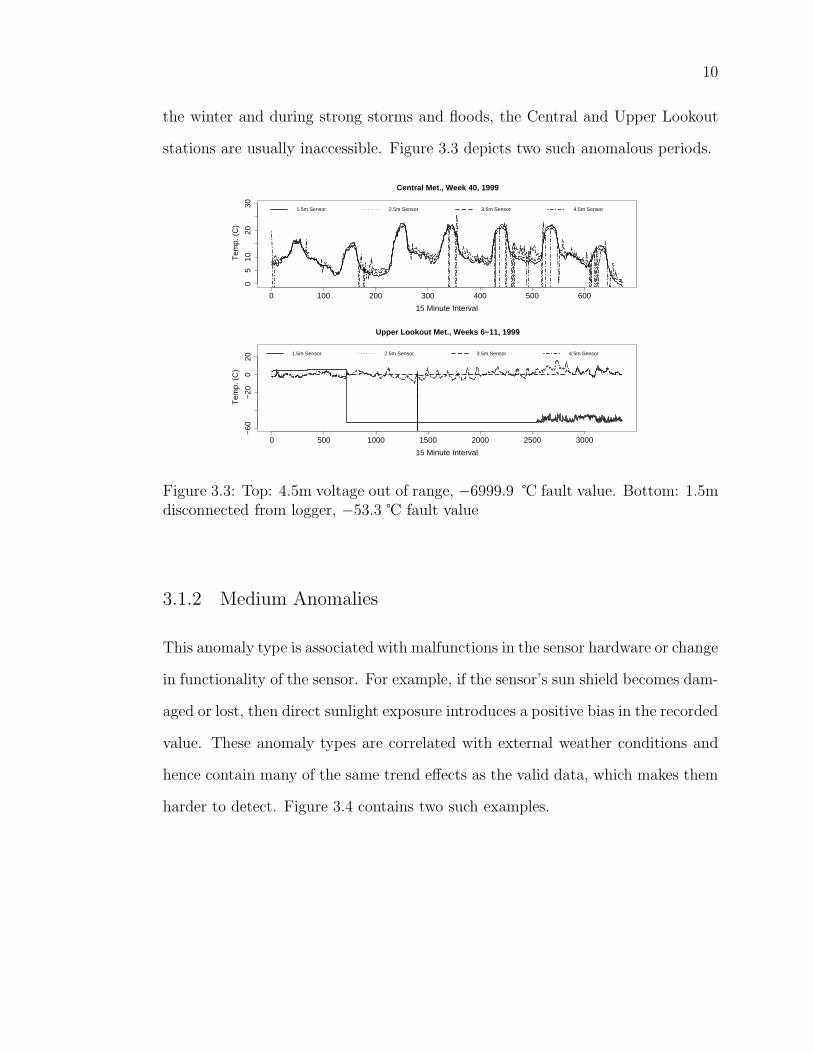
the winter and during strong storms and floods, the Central and Upper Lookout

stations are usually inaccessible. Figure 3.3 depicts two such anomalous periods.

0 100 200 300 400 500 600

05

1020

30

Central Met., Week 40, 1999

15 Minute Interval

Tem

p. (

C)

1.5m Sensor 2.5m Sensor 3.5m Sensor 4.5m Sensor

0 500 1000 1500 2000 2500 3000

−60

−20

020

Upper Lookout Met., Weeks 6−11, 1999

15 Minute Interval

Tem

p. (

C)

1.5m Sensor 2.5m Sensor 3.5m Sensor 4.5m Sensor

Figure 3.3: Top: 4.5m voltage out of range, −6999.9 ℃ fault value. Bottom: 1.5mdisconnected from logger, −53.3 ℃ fault value

3.1.2 Medium Anomalies

This anomaly type is associated with malfunctions in the sensor hardware or change

in functionality of the sensor. For example, if the sensor’s sun shield becomes dam-

aged or lost, then direct sunlight exposure introduces a positive bias in the recorded

value. These anomaly types are correlated with external weather conditions and

hence contain many of the same trend effects as the valid data, which makes them

harder to detect. Figure 3.4 contains two such examples.

11

0 100 200 300 400 500 600

05

1020

30

Central Met., Week 6, 1996

15 Minute IntervalT

emp.

(C

)

1.5m Sensor

2.5m Sensor

3.5m Sensor

4.5m Sensor

0 500 1000 1500 2000 2500

−10

05

1020

Upper Lookout Met., Weeks 3−7, 1996

15 Minute Interval

Tem

p. (

C)

1.5m Sensor

2.5m Sensor

3.5m Sensor

4.5m Sensor

Figure 3.4: Top: Broken Sun Shield, Bottom: 1.5m Sensor buried under snowpack,2.5m Sensor dampened

The first plot illustrates the loss of a sun shield on the 1.5m sensor, which

raises the recorded temperature by approximately 5 ℃. It is important to note

that this bias disappears during the night time periods and also on cloudy days

(which probably explains why the bias is missing during the last two days of the

week).

The second plot results from a snowpack that has buried the 1.5m sensor by

the 200th quarter-hour measurement. This sensor records the temperature as a

near-constant −2 ℃ for approximately 3 weeks. Notice that the 2.5m sensor is also

affected by the snow: its diurnal behavior is significantly dampened. Indeed, we can

observe that the snow first buries the 1.5m sensor before affecting the 2.5m sensor

and that, as the snowpack melts, the 2.5m sensor returns to nominal behavior

12

before the 1.5m sensor. This behavior is consistent with snowpack accumulation

and thawing.

In addition to these two sensor malfunctions, there are cases where very infre-

quent voltage errors can cause effects similar to the sunshield loss. The recorded

15-minute temperature reading at the logger is actually an average of readings

taken by the air temperature sensor every 15 seconds. If at any point during the

15 minutes the sensor becomes disconnected or reports out of the voltage range,

these bad values can be averaged into a series of good readings, resulting in a

mixed error type.

3.1.3 Complex Anomalies

We reserve this classification for anomalies that are so subtle that they cannot be

captured without the use of additional sensors. An example of a complex anomaly

is a switch in sensor cables between two adjacent sensors on a tower. Because

under normal conditions the two sensor readings differ by only a fraction of a

degree Celsius, if we examine only one of the sensor streams, we cannot detect

the anomaly. However, a model of the joint distribution of all four sensors on

the tower should be able to capture the fact that the relative order of the sensor

values reflects their physical order on the tower. Specifically, the 4.5m sensor is the

hottest of the four in the mid-afternoon and the coolest of the four in the middle

of the night. Because the present work only models individual sensor streams, we

do not expect it to detect these complex anomalies.

13

Chapter 4 – Hybrid Bayesian Networks

Our generative model of the air temperature domain is a conditional linear-Gaussian

network, also known as a hybrid network due to the presence of both continuous

and discrete variables [16, 22]. For the sake of computational convenience, we will

only consider continous variables represented by a Gaussian distribution, and only

networks where continuous variables have some mixture of discrete and continuous-

valued parents and discrete variables have only discrete-valued parents. Discrete

variables with continuous-valued parents (represented by a logit distribution) are

discussed in further detail in Murphy [23].

4.1 Conditional Gaussian

Consider a single continuous variable, X, represented by the Gaussian distribution

X ∼ N (µ, σ2). For every possible instantiation of values for the discrete parents

of X, there is an accompanying parameterization of X; specifically, a separate µ

and σ2. For example, if X has a single boolean parent, Y = y ∈ {true, false},

then the conditional probability table (CPT) of X would contain two entries:

P (X|Y = true) ∼ N (µt, σ2

t ) and P (X|Y = false) ∼ N(

µf , σ2

f

)

. In general, let

Y = {Y1, Y2, ..., Yn} denote the set of discrete parents of the continuous variable X.

Further, let |Y| = |Y1|×|Y2|× ...×|Yn| be the total size (number of possible instan-

14

tiations) of Y. Then, we specify the CPT of X with the |Y| dimensional vector,

~µ =⟨

µ1, µ2, ..., µ|Y|

⟩

. Similarly, we specify the set of possible variances assumable

by X, depending on the parent configuration, as the vector ~σ2 =⟨

σ2

1, σ2

2, ..., σ2

|Y|

⟩

.

Figure 4.1 contains an example with binary discrete variables.

X

Y2Y1 Yi Yn-1 Yn… … yi P(Yi=y)

true p

false 1-p

Y1 Y2 …. Yn

true

true

… ... false false … …

false false false false µ2n

true

22n

truetrue

false….true

µ 2

µ121

µ222

Figure 4.1: Conditional Gaussian Network

4.2 Linear Gaussian

Again, consider a single continous variable, X, parameterized as above. For each

continuous-valued parent, Zi ∈ Z = {Z1, Z2, ..., Zm}, X has an additional regres-

sion weight, wi, such that mean of X is now calculated:

µx = ǫ +m

∑

i=1

wizi (4.1)

15

where zi is a value drawn from the Gaussian parent, Zi, and ǫ is essentially X’s

constant mean in the linear regression formula. The variance of X is still specified

by a single σ2 parameter and is not conditioned on the parents.

4.3 Conditional Linear-Gaussian

As the name suggests, a conditional Linear-Gaussian (CLG) node is simply a

combination of the previous two variable types. Let X be a continuous variable

with a set of discrete parents, Y, and continuous parents, Z, as defined above.

That is, X has a separate mean, variance, and set of regression weights for each

possible instantion of Y. We specify a CLG variable with a mean vector, ~µ =⟨

µ1, µ2, ..., µ|Y|

⟩

, a variance vector (again, really just the diagonal of the covariance

matrix), ~σ2 =⟨

σ2

1, σ2

2, ..., σ2

|Y|

⟩

, and a |Y| × |Z| regression matrix:

w1,1 w1,2 ... w1,|Z|

w2,1 w2,2 ... w2,|Z|

w...,1 w...,2 ... w...,|Z|

w|Y|,1 w|Y|,2 ... w|Y|,|Z|

(4.2)

Figure 4.2 contains a trivial CLG network with a continuous variable having a

single discrete and continuous parent.

16

Y

X

Z

y P(Y=y)

true p

false 1-p

),(~2

zzNZ

Y P(X|Y=y, Z=z)

true ~N(µ1,x+ w1,z * z,21)

false ~N(µ2,x+ w2,z * z,22)

Figure 4.2: Conditional Linear-Gaussian Network

17

Chapter 5 – Domain Model

We construct a Conditional Linear Gaussian (CLG) DBN to model the interaction

between a single sensor and the air temperature process. Each slice of the tem-

poral model represents a fifteen-minute interval, as this is the time granularity of

our sensor observations. However, our model also contains two observed discrete

variables representing the current time window:

1. QH = 1, ..., 96 Representing the current quarter-hour of the day

2. Day = 1, ..., 365 Representing the current day of the year.

Thus, every slice is associated with a unique (QH = qh, Day = d) pair. The in-

tuition behind this is that, as in the case of the PAR model, we would like to

model more rapid or slower fluctuations in temperature depending on periods of

the weather cycle (both diurnal and seasonal). Further discussion will be divided

into the process model governing air temperature change and the model for sensor

behavior.

5.1 The Process Model

For any given time step and (qh, d), we assume the actual temperature, T , is a

function of some learned baseline value, B (please see section 5.1.1 for discussion of

18

the baseline value) and a value representing the current departure from the baseline

value, ∆. That is, we estimate the distribution over T : T ∼ N (∆ + B, σ2

T ) .

The ∆ variable can be interpreted as representing a temporally local trend

effect, such a warm/cold front or a storm. Its purpose is to capture the dif-

ference between our baseline expectation for the temperature at a given time of

day/day of year and the observed temperature during periods of nominal sensor

behavior. We model ∆ as a first-order Markov process with the current (qh, d)

as additional non-Markovian, observed inputs. Thus, ∆ has the distribution

∆ ∼ N(

µqh,d + w∆t−1, σ2

qh,d

)

. The Markov process allows the ∆ distribution

to “wander” in order to capture growing or diminishing trend effects. By condi-

tioning the distribution on QH and D, we can account for sharper temperature

shifts associated with particular (qh, d) pairs. For example: the temperature rises

and falls more quickly as a result of diurnal effects in summer months than in

winter months. To account for this, ∆ must be able to change more rapidly (have

increased variance) during these periods of the day and season.

5.1.1 Calculating the Baseline

The baseline value for a particular (qh, d) pair estimates the temperature for that

time interval after removing short-term trends due to weather systems. Initially,

it may seem appropriate to simply average temperature values for a given (qh, d)

pair across all of the training years. However, as we have only a few training

years, there is too much variance in sample means to provide a good estimate. To

19

t

QH Day

B

T

1t …

}96,...,1{QH

}365,...,1{Day

),(~2

,1, dqhtdqht N

),(~2

Tt BNT

Figure 5.1: Process model for air temperature. Rectangles depict discrete variables,ovals depict normally distributed variables. Shaded variables are observed.

address this, we apply a moving average kernel smoother across the M days on

either side of the current day and the N quarter-hour periods on either side of the

current quarter hour. However, if we only used this simple smoother, it would be

biased low at times when the second derivative of the temperature was negative

(at the point of maximum temperature) and biased high at times when the second

derivative of the temperature was positive. To correct for this, we compute the first

derivative Q(d, qh, t, y) for each (u, t) offset, and use this to remove the short-term

linear trend in the temperature curve:

Bqh,d = c∑

y,u,t

T (d + u, qh + t, y) − Q (d, qh, t, y) (5.1)

c = [Y (2M + 1) (2N + 1)]−1 (5.2)

20

where y ∈ {1, ..., Y } denotes the year index, u ∈ {−M, ..., M} denotes the day off-

set, t ∈ {−N, ..., N} denotes the quarter-hour offset, and T (d, qh, y) is the training

value for a given (d, qh, y) tuple.

Q (d, qh, t, y) is the first-derivative offset function that calculates the average

deviation from the current quarter-hour to t over a 2M + 1 day window. It is

calculated as:

Q (d, qh, t, y) = (2M + 1)−1∑

u

T (d + u, qh + t, y) − T (d + u, qh, y) . (5.3)

Figure 5.2 shows this algorithm applied to a week-long sliding window in the

calculuation of a single point of the baseline (note that this value would then be

averaged across all training years instead of the single year shown).

23600 23700 23800 23900 24000 24100

-50

510

15

20

25

30

Central Met. Week 35, 2006

15 Minute Interval

Tem

p.

(C)

TemperaturesTemperatures

Offset

23600 23700 23800 23900 24000 24100

-50

510

15

20

25

30

Central Met. Week 35, 2006

15 Minute Interval

Tem

p.

(C)

23600 23700 23800 23900 24000 24100

-50

510

15

20

25

30

Central Met. Week 35, 2006

15 Minute Interval

Tem

p.

(C)

Baseline value

Figure 5.2: Computation of Baseline Value over Week-long Window.

The offset for the 2N + 1 length quarter-hour window is first calculated by

taking the difference between each quarter-hour in that window and the current

21

(qh, d) value for which we are calculating the baseline, and then averaging that

difference across all days in the 2M + 1 day window. This offset will be centered

around 0, as indicated in the figure. Next, we subtract this offset value (which

will be the same across all 2M + 1 days) from the observed values in our window.

The result of this is the detrended data should resemble a relatively flat segment

for each day in the window (shown in the figure as intersecting with the training

data). The baseline value is then calculated as the average of all detrended values

for the day and quarter-hour window.

5.2 Sensor Model

Based on our discussions with the expert, we have identified several anomaly types

in the temperature data streams. However, we are not confident that we have

found all anomaly types. Each time we meet with the expert, we learn about a

new anomaly, and there is no reason to expect that the set of anomalies is fixed.

Hence, rather than attempting to model each type of anomaly separately, which

would lead to a system that could only recognize a fixed set of anomaly types, we

decided to develop a single, very general fault model that is able to capture most

of the known anomaly types and (we hope) unknown types as well. We model the

state of the sensor, S, as a discrete variable that summarizes the degree of sensor

functionality. We chose four levels of sensor quality at the behest of the domain

expert to discriminate between slightly erroneous values (which may still have some

use) and truly erroneous values. The state S is modeled as a first-order Markov

22

process, which allows us to capture the fact that good sensors tend to stay good

and bad sensors tend to stay bad. The observed temperature, O, is distributed as

N(µs+wsT, σ2

s), where the values of σ2

s capture how well the observed temperature

is tracking the true temperature as a function of the current state S = s. Figure

5.3 depicts the full domain model.

t

QH Day

BT

1t

tS1tS

O

…

…

Figure 5.3: Integrated single-sensor and process model.

23

Chapter 6 – Methods

We obtained eleven years of raw air temperature from the H. J. Andrews Ex-

perimental Forest (1996 - 2006). This data had been processed by the domain

expert to mark all anomalous data points. The domain expert has a tendency to

overlabel data; a long time interval may be labeled as anomalous even though it

contains some short time intervals where the data is not anomalous. This behavior

is predominately observed on medium-type anomalies, where it can be difficult to

discern isolated anomalies at the 15-minute time granularity. For example, if a

sun shield was missing, the expert would mark the entire time interval when the

shield was missing as anomalous even though at night time and on cloudy days

the temperature readings are accurate.

6.1 Model Parameterization

For each of the three meteorological stations, we selected four years of data as our

training set. From this set, we removed all data points labeled anomalous by the

expert and trained on the remaining data. We calculated a baseline value for every

(qh, d) pair as described in section 5.1.1, with the number of days M = 3 and the

number of quarter hours N = 5. Using these values, we then iterated through the

24

training set and calculated the following:

∆(y, d, qh) = T (y, d, qh)− B(d, qh), (6.1)

where T (y, d, qh) is the recorded temperature for that year, day, and quarter-hour,

and B(d, qh) is the baseline value.

To fit the conditional distribution for ∆, we smooth over a 31-day window. We

compute the mean and variance of ∆qh,d as

µqh,d = (Y M)−1∑

y,u

∆(y, d + u, qh) − ∆(y, d + u, qh − 1) (6.2)

σ2

qh,d = (Y M)−1∑

y,u

(∆(y, d + u, qh) − µqh,d)2 (6.3)

where Y = 4 is the number of years, and M = 31 is the number of days.

We manually tuned the parameters for the predicted temperature (T ), the ob-

served temperature (O), and the sensor (S) variables to implement the generic fault

model. The sensor can be in one of four states: {Very Good, Good, Bad, Very Bad}.

The first three states assert equality between the mean of the predicted and ob-

served temperatures, and the last state encompasses anomalies in which the ob-

served temperature is completely independent of T . We impose this artificial gra-

dient of sensor qualities so that end users can make a more informed choice with

regards to the data quality they wish to use. That is, a binary labeling system

{Good, Bad} may dissuade a user from using any data labeled Bad even though

the degree of error may be trivial, as in the case of sensor-swapped data.

25

Table 6.1: Observed Temperature as a function of Sensor State and PredictedTemperature

SENSOR STATE DISTRIBUTION

O|St = V eryGood N (T, 1.0)O|St = Good N (T, 5.0)O|St = Bad N (T, 10.0)

O|St = V eryBad N (0, 100000)

We calculate the actual temperature as the sum of the baseline and the current

∆ offset. We assign weights of 1.0 for both these variables and set ∆’s mean to

0. Further, we supply ∆ with a very low, non-zero variance. The distribution

over the observed temperature is tied to the state of the sensor, and thus we can

use the sensor state to explain large residuals between the observed and predicted

temperature. In cases where the sensor is believed to be functioning nominally,

the observed temperature should be the predicted temperature with some minimal

variance. If we believe the sensor is malfunctioning, we allow the observed tem-

perature to take on additional variance yet still reflect the mean of the predicted

temperature. In cases where we believe the sensor is completely failing, we set the

weight from the predicted temperature to 0, and we assign a huge variance to O.

Table 6.1 displays the distribution of O given the state of S.

26

6.2 Model Simulation

We perform inference in our network using a variation on the Forward Algo-

rithm [26, 29] and Bucket Elimination adapted for CLG networks [7, 8, 15]. The

Forward Algorithm computes the marginal for every step of a Markov process and

passes that distribution forward as the alpha message. The Bucket Elimination

algorithm is a dynamic-programming, exact-inference method that represents po-

tentials as buckets and marginalizes out variables iteratively until only the desired

potential remains.

Table 6.2 outlines our modified Forward inference method. The two modi-

fications to the Forward algorithm occur in steps 3 and 5. In 3, we enforce a

decision about the state of the sensor and use its most likely value to constrain

the distribution on ∆ computed in 4. In other words, at each step, we compute

the posterior distribution over S and then force S to take on its most likely value.

This is necessary to prevent the variance associated with ∆ from growing rapidly.

Consider the elimination ordering in Table 6.3. The potential in (1) will fail

to sufficiently constrain the variance of ∆t, because there is always a non-zero

probability that St = Very Bad. The high variance associated with the general

fault state of the sensor then removes the constraining effect the observation O

provides. By entering evidence for the sensor state before computing the posterior

of ∆t, we eliminate this problem. The additional observation for St changes the

expression in (1) to:

P (O = o|St = s, T )P (T |B = b, ∆t) = Pot(∆t) (6.4)

27

Table 6.2: Modified Forward Algorithm

1. Enter evidence for observed variables: QH, Day, B, and O

2. Compute the posterior for St as the new alpha message, αS

3. Enter the most likely value of St, argmaxs

P (St = s|O1:t) for

time t and as additional evidence.

4. Compute posterior for ∆t as the new alpha message, α∆

5. If s = Very Bad, then set variance of α∆ to min(

σ2

qh,d, σ2x

)

where σ2

qh,d is the regular variance of ∆ for that (qh, d) pair

and σ2x is the calculated variance of α∆

6. Update St−1 to αQ and ∆t−1 to α∆ (pass α messages for-ward) and return to 1.

and removes the potential calculated in (4). Pot(∆t) sufficiently constrains ∆t’s

variance for all values of st except Very Bad. We address the latter case in step

5 of our algorithm (Table 6.2) by setting an upper limit on the variance of the

posterior. The limit is the trained variance parameter for ∆ for the current (qh, d)

pair.

6.3 Inference in CLG Networks

As mentioned in 6.2, we perform exact inference in our model using a Vari-

able/Bucket Elimination algorithm adapted to CLG networks. We outline the

inference process in hybrid networks here; however, we refer the reader to Lau-

28

Table 6.3: Bucket Elimination for P (∆t) Elimination Ordering: T, ∆t, St, S

P (O = o|St, T )P (T |B = b,∆t) = Pot (∆t|St) (6.5)

P (∆t|∆t−1) P (∆t−1) = Pot (∆t) (6.6)

P (St|St−1) P (St−1) = Pot (St) (6.7)

Pot (∆t|St) Pot (St) = Pot (∆t)′

(6.8)

Pot (∆t)Pot (∆t)′

(6.9)

ritzen and Murphy [15, 16, 22] for a more thorough explanation.

Recall that in Variable Elimination, first an elimination ordering is determined

either at random (as in our case) or in such a way as to minimize the induced width

of any potential (a known NP-Hard problem, [2]). The algorithm then iterates

through each variable in the elimination list. For each iteration, the algorithm

combines all variables related to the current variable in the list into a bucket by

taking the pointwise product of all variables’ CPTs and then eliminates the current

variable through marginalization. We will refer to merged CPTs in a bucket as a

potential, denoted Pot (x1, x2, ..., xn), where x1, x2, ..., xn refers to the variables in

the bucket.

Prior to any computation, we first represent each variable’s CPT in terms of

its canonical characteristics, g,h, and K. For the Normal distribution (univariate

case), these characteristics are computed from the CLG parameters (section 4.3)

29

as the following:

g = −µ2

2σ2−

1

2log

(

2πσ2)

(6.10)

h =µ

σ2

−w

1

(6.11)

K =1

σ2

wwT −w

−wT 1

(6.12)

Note that w is a vector of weights associated with the LG or CLG variable, so h

will be a vector of size of |w| + 1 and K will be a (|w| + 1) × (|w| + 1) matrix.

For the discrete variables, we replace each entry in the variable’s CPT with

the canonical formulation of its probability, which is simply g = log p where p

is probability value. h and K are initialized as an empty vector and matrix,

respectively.

6.3.1 Product & Marginalization

Once all CPTs are represented by their canoncial characeristics, multiplying two

CPTs is a two-step process. Let us consider the product between two CPTs

(or potentials), denoted φ1 and φ2, over the sets of variables {x1, x2, ..., xn} and

{y1, y2, ..., ym}, respectively. Recall that the resultant pointwise product of φ1×φ2

will be a potential over the union of the variables in φ1 and φ2, {x1, ..., xn, y1, ..., ym}.

Thus, our first step is to extend the domain of the canonical characteristics of φ1

30

and φ2 such that they now include all variables in the aforementioned union. This

is done by inserting rows or columns of zeros into the h and K components ac-

cordingly. Next, the product of φ1 and φ2 is then simply computed as:

(g1,h1, K1) ∗ (g2,h2, K2) = (g1 + g2,h1 + h2, K1 + K2) . (6.13)

Once all CPTs in a bucket have been multiplied, the current variable in the elim-

ination ordering must be marginalized from the potential. If the variable being

marginalized is continuous-valued, this is done by first breaking the h and K

canonical components of the potential into distinct sections as follows:

h =

h1

h2

(6.14)

K =

K11 K12

K21 K22

(6.15)

where h1 refers to the index of the variable to-be-eliminated in the list of continu-

ous variables in the potential, and h2 denotes the remaining continuous variables.

Similarly, K11 refers to the row and column index of the variable to-be-eliminated

in the K matrix, K12 is the K matrix minus the column containing the variable,

K21 is the matrix minus the row containing the variable, and K22 is the K matrix

minus both the row and column containing the variable. Finally, the new canonical

31

characteristics representing the marginalized potential are calculated as follows:

g = g +1

2

(

p log (2π) − log |K11| + hT1K−1

11h1

)

(6.16)

h = h2 − K21K−1

11h1 (6.17)

K = K22 − K21K−1

11K12 (6.18)

where p is the dimension or length of the vector h1. In the case of marginalizing

a discrete variable, we approximate the mixture of Gaussians by reducing the

mixture into a single component. This process is done with the moment form of

the potential:

p (i) =∑

j

p (i, j) (6.19)

µ (i) =∑

j

µ (i, j) p (i, j) /p (i) (6.20)

Σ (i) =∑

j

Σ (i, j) p (i, j) /p (i) + (6.21)

∑

j

(µ (i, j) − µ (i)) (µ (i, j) − µ (i))T p (i, j) /p (i) , (6.22)

where j refers to instantations of the discrete variable being summed out. Because

the inverse of the product of two covariance matrices may not always be well-

defined, we avoid working in the moment form until absolutely necessary. We

do this by enforcing a strong triangulation [14] elimination ordering that always

eliminates continuous-valued variables before discrete. This insures that when

we do perform margninalization over a discrete variable, all products involving

32

Gaussian variables have already been performed.

33

Chapter 7 – Results

We evaluate our method over seven years of labeled data from the H.J. Andrews

while holding out four years for training. Training and testing years were individu-

ally selected for each site with a preference for years including few or no anomalies

in the training set, and years exhibiting the largest diversity of anomaly types in

the test set. We analyze our results in terms of anomaly difficulty and then intro-

duce an additional classification method designed to approximate the behavior of

the domain expert. Finally, we report overall precision and recall with regard to

our classification system and each meteorological station.

7.1 Simple Anomaly Types

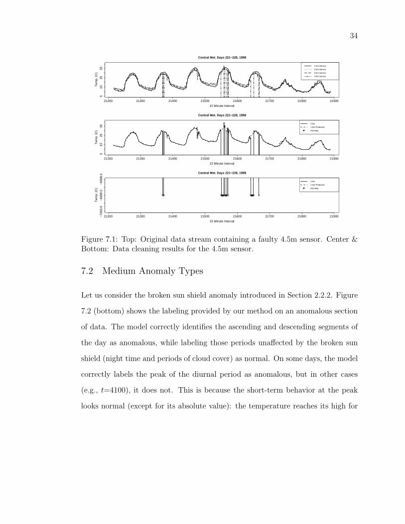
Figure 7.1 shows a typical result provided by the model for intermittent sensor

faults associated with a voltage error in the sensor. Plotted points indicate points

labeled as anomalous (Bad or Very Bad) by our system. We omit the Good and

Very Good labels for clarity. Note that all values of −6999.9 ℃ were correctly

labeled as Very Bad ; also, the model produced no false positives for the week

shown. The predicted temperature values inserted (the dotted line) in place of

those labeled anomalous closely resemble the neighboring valid segments of the

data stream.

34

21200 21300 21400 21500 21600 21700 21800 219005

1525

35

Central Met. Days 221−228, 1998

15 Minute Interval

Tem

p. (

C)

1.5m Sensor

2.5m Sensor

3.5m Sensor

4.5m Sensor

21200 21300 21400 21500 21600 21700 21800 21900

515

2535

Central Met. Days 221−228, 1998

15 Minute Interval

Tem

p. (

C)

1.5m

1.5m Predicted

Anomaly

21200 21300 21400 21500 21600 21700 21800 21900−70

00.0

−69

99.0

−69

98.0

Central Met. Days 221−228, 1998

15 Minute Interval

Tem

p. (

C)

1.5m

1.5m Predicted

Anomaly

Figure 7.1: Top: Original data stream containing a faulty 4.5m sensor. Center &Bottom: Data cleaning results for the 4.5m sensor.

7.2 Medium Anomaly Types

Let us consider the broken sun shield anomaly introduced in Section 2.2.2. Figure

7.2 (bottom) shows the labeling provided by our method on an anomalous section

of data. The model correctly identifies the ascending and descending segments of

the day as anomalous, while labeling those periods unaffected by the broken sun

shield (night time and periods of cloud cover) as normal. On some days, the model

correctly labels the peak of the diurnal period as anomalous, but in other cases

(e.g., t=4100), it does not. This is because the short-term behavior at the peak

looks normal (except for its absolute value): the temperature reaches its high for

35

the day, it holds steady for a short period, and then begins to decrease. The reduced

rate of change in temperature between time slices then falls within the range of

∆’s variance, so it is labeled as non-anomalous. Note that the model-predicted

temperature slightly lags the observed 4.5m temperature. This matches the 1.5m,

2.5m, and 3.5m sensors, which are labeled by the domain expert as functioning

nominally for this period and corrects for the incorrect acceleration/deceleration

introduced by the fault.

4100 4200 4300 4400 4500 4600 4700

05

1020

30

Central Met. Week 6, 1996

15 Minute Interval

Tem

p. (

C)

1.5m Sensor

2.5m Sensor

3.5m Sensor

4.5m Sensor

4100 4200 4300 4400 4500 4600 4700

05

1020

30

Central Met. Week 6, 1996

15 Minute Interval

Tem

p. (

C)

1.5m

1.5m Predicted

Anomaly

Figure 7.2: Top: Lost sun shield in 1.5m sensor. Bottom: Data cleaning appliedto 1.5m sensor.

7.3 Class Widening

As a result of working at very fine time granularities, the domain expert tends to

“over-label” faults (i.e., marking long segments as faulty even though only some of

36

the points in those segments are actually faulty). We correct for this behavior when

directly comparing our classification to the expert’s by introducing a widening

method. For any point labeled as anomalous (Bad or Very Bad) by both the

expert and our system, we widen our classification by assigning the same class to

λ points before and after the current quarter hour. We apply this widening only to

those anomalous types we consider to be non-trivial, as the expert is very precise

in labeling of extreme anomalies (out of voltage range, sensor disconnects, etc.).

7.4 Precision and Recall

Figure 7.3 displays the precision and recall results for each of the meteorological

stations over a range of λ values for the aforementioned widening method. The

diamond-marked line represents the average performance among all three sites.

The benefit gained from the application of class widening is largely dependent

on the types of anomalies encountered at each site. For example, the Central Met

station benefits the most from widening because that site contained many medium-

type anomalies (broken sun-shield predominately), which tend to be over-labeled

in manual inspections. The class widening method allows us to tune our system to

simulate the domain expert labeling (obtain higher recall rates) at the cost of our

false positive rate. For example, by increasing λ from 0 (individual labeling) to 200

(2-day window on either side of the current quarter hour), we have increased our

average recall from 61% to 78%; however, we have done so at the cost of increasing

our false positive rate from 2.1% to 3.2%. Our results indicate that λ = 70 provides

37

the highest precision score before beginning to decline as a result of increased false

positives rates. At this λ value, we achieve an average precision, recall, and FPR

across all testing sets of 38%, 73%, and 2.5%, respectively. However, these overall

numbers hide many different situations, so we will analyze our results with respect

to the precision and recall values obtained at each meteorological station.

0 100 200 300 400

0.1

0.2

0.3

0.4

0.5

Precision

1/2 Window Width

Pre

cisi

on

●

●● ● ● ● ● ● ● ● ● ● ● ● ● ● ● ● ● ● ●

● Central

Upper Lookout

Primary

Average

0 100 200 300 400

0.4

0.5

0.6

0.7

0.8

0.9

1.0

Recall

1/2 Window Width

Rec

all

●

●

●

●●

●●

●●

● ● ● ● ● ● ● ● ● ● ● ●

● Central

Upper Lookout

Primary

Average

Figure 7.3: Precision and Recall as a function of λ. Marked increments of 100.

7.5 Central Meteorological Station

Figure 7.4 displays a scattergram of the results of our classification method (λ =

70) applied to the Central Met test sets. The comma-separated values below each

circle relate the sensor (1, 2, 3, and 4 referring to the 1.5m, 2.5m, 3.5m, and 4.5m

sensors) and test year (1996, 1997, 1998, 2001, 2002, 2003, 2004).

38

0.0 0.2 0.4 0.6 0.8 1.0

0.0

0.2

0.4

0.6

0.8

1.0

Precision vs. Recall, Central Met Station

Precision

Rec

all

1, 1996

1, 1997 1, 19981, 20011, 20021, 2003 1, 2004

2, 1996

2, 19972, 19982, 2001

2, 2002

2, 2003

2, 2004

3, 1996

3, 19973, 1998

3, 2001 3, 2002

3, 2003

3, 2004

4, 1996

4, 1997

4, 1998

4, 2001

4, 20024, 2003 4, 2004

(a)

(b)

Figure 7.4: (a) Infrequent, simple anomalies and (b) long-term sensor swaps.

The region denoted as (a) contains years having infrequent, short-duration,

simple anomalies. 11 of the 28 data sets from Central Met fall into this category.

They contain very few actual anomalies (median = 3), which are easily detected

by system (recall rates of 100% are obtained on these data sets). Unfortunately,

because these anomalies are so sparse, our precision rate is adversely affected by

our false positive rate. Even our modest false positive rate of 1.9% (approximately

666 FP’s per 35040 values in a data set) dominates our precision score. These

numbers are still very good. Our goal is to produce a system that can be used as

a filter to focus the time and attention of the domain expert on those points most

likely to be anomalous. Consequently, if the expert examines all of the points that

39

we predict to be positive, this will reduce by 98% the number of points that must

be examined while still detecting all true anomalies. As we move right across the

x-axis, we see our precision rates improve on data sets that contain more frequent

simple anomaly types.

As we move down the y-axis from (a), we come across data sets that still

contain few anomalies, but the anomaly type is less clear. In the extreme case, the

2.5m and 3.5m sensors from Central 1996 both contain a single labeled anomaly

that appears entirely consistent with neighboring values, and is misclassified by

our system. The region in (b) contains data sets almost entirely dominated by

anomalous values (median = 30565.5); these are probably values expunged from

the database due to swapped sensor leads. We obtain high precision on these sets

because essentially any value we classify as anomalous was labeled as such by the

expert. Similarly, our poor recall scores on these sets is a result of the fact that

much of the data looks completely normal, and our system is as-of-yet unable to

detect swapped sensor leads. The remaining data sets populating the scatterplot

represent a trade off between the two regions denoted in (a) and (b). That is,

they tend to be data sets containing medium anomaly types (sun shield failures,

voltage-range errors) of increasing duration as we move right across the x-axis and

more obvious as we move up the y-axis.

Tables 7.1 and 7.2 contain anomaly counts and accuracy scores (percent of

points classified by our system correctly) for each data set at the Central Met

station using our class-widening technique with λ = 70. With the exception of

the 4 data sets denoted in (b), we tend to achieve fairly high accuracy scores.

40

Year 1.5m 2.5m 3.5m 4.5m

1996 2537.0 1.0 1.0 4.01997 302.0 0.0 0.0 2.01998 984.0 13.0 13.0 4420.02001 3.0 3.0 68.0 8.02002 3.0 5512.0 5890.0 19.02003 2.0 35040.0 35040.0 0.02004 1369.0 26091.0 26091.0 1369.0

Table 7.1: Anomaly Counts for Central Met sensors

Year 1.5m 2.5m 3.5m 4.5m

1996 0.9473 0.9860 0.9804 0.99091997 0.9680 0.9858 0.9829 0.99201998 0.9797 0.9895 0.9902 0.92792001 0.9656 0.9769 0.9664 0.98592002 0.9660 0.8393 0.8672 0.98712003 0.9602 0.2678 0.1322 0.99532004 0.9615 0.4706 0.3871 0.9905

Table 7.2: Accuracy scores for Central Met sensors

Moreover, we maintain low false-positive rates for the data sets while achieving an

average recall of 69% (the sets in (b) taken into account).

7.6 Primary Meteorological Station

Figure 7.5 displays a scattergram of the results of our classification method (λ =

70) applied to the Primary Met test sets. As in figure 7.4, the comma separated

values detail the sensor and year of the test set. Note that the labels have been

omitted from the sets in (a) for the sake of clarity.

The region in (a) represents the set of test sets similar to those in Figure 7.4 (a);

41

Year 1.5m 2.5m 3.5m 4.5m

1996 0.0401 0.0139 0.0195 0.00891997 0.0321 0.0141 0.0170 0.00791998 0.0208 0.0104 0.0097 0.00632001 0.0343 0.0230 0.0323 0.01392002 0.0339 0.0214 0.0270 0.01292003 0.0397 0.0 0.0 0.00462004 0.0400 0.0408 0.0098 0.0098

Table 7.3: False positive rates for Central Met sensors

that is, years containing infrequent, short-term anomalies that are of the simple

type. There are 13 such data sets in the Primary Met station with a median

anomaly count of 74, in which we obtain precision scores ≤ .2 and recall scores ≥

.8. The data sets enclosed in (b) contain a mixture of simple anomaly types like

those in (a), some short periods of sensor disconnects, as well as several voltage-

related anomaly types. Our precision scores increase on these 10 data sets for

many of the same reasons they increased on the Central Met sets; the anomaly

types are easily detected by our system, and the abundance of these anomalies

(median=626) begins to compensate for our false-postive rate. Finally, the four

sets from sensors 3 and 4 for years 2003 and 2004 contain sensor swaps, resulting

in higher precision scores and, ufortunately, reduced recall. Tables 7.4, 7.5, and

7.6 display the anomaly counts, accuracy scores, and false positive scores for the

Primary Met testing sets.

42

Year 1.5m 2.5m 3.5m 4.5m

1998 721.0 626.0 626.0 626.02000 569.0 474.0 472.0 1153.02001 149.0 70.0 70.0 70.02002 1.0 11016.0 11016.0 1.02003 10.0 17914.0 35040.0 11.02004 100.0 99.0 4282.0 100.02006 1456.0 154.0 154.0 584.0

Table 7.4: Anomaly Counts for Primary Met sensors

Year 1.5m 2.5m 3.5m 4.5m

1998 0.9793 0.9813 0.9803 0.98052000 0.9662 0.9705 0.9723 0.97152001 0.9723 0.9767 0.9726 0.96832002 0.9702 0.7547 0.7690 0.96842003 0.9816 0.6258 0.1898 0.97312004 0.9686 0.9718 0.8630 0.96802006 0.9580 0.9561 0.9612 0.9698

Table 7.5: Accuracy scores for Primary Met sensors

Year 1.5m 2.5m 3.5m 4.5m

1998 0.0206 0.0188 0.0197 0.01952000 0.0342 0.0298 0.0280 0.02942001 0.0276 0.0233 0.0273 0.03172002 0.0297 0.0455 0.0496 0.03152003 0.0183 0.0188 0.0 0.02682004 0.0314 0.0281 0.0295 0.03192006 0.0437 0.0440 0.0389 0.0306

Table 7.6: False positive rates for Primary Met sensors

43

0.0 0.2 0.4 0.6 0.8 1.0

0.0

0.2

0.4

0.6

0.8

1.0

Precision vs. Recall, Primary Met Station

Precision

Rec

all

1, 19981, 2000 1, 20062, 19982, 2000

2, 20022, 2003

3, 19983, 2000

3, 2002

3, 2003

3, 2004

4, 1998 4, 20004, 2006

(a)(a) (b)

Figure 7.5: (a) Infrequent, simple anomalies and (b) semi-frequent simple &medium anomalies.

7.7 Upper Lookout Meteorological Station

Figure 7.6 displays a scattergram of the results of our classification method (λ =

70) applied to the Upper Lookout Met test sets. As in the previous two scat-

tergrams, the comma separated values detail the sensor and year of the test set.

Again, the labels have been omitted from the sets in (a) for the sake of clarity.

The section in (a) represents those data sets (8 in total) with few (median = 6),

easily detected anomalies.

Upper Lookout, located at the highest altitude of the three stations, often

receives enough cumulative snowfall to damage low-lying sensors on the tower

44

0.0 0.2 0.4 0.6 0.8 1.0

0.0

0.2

0.4

0.6

0.8

1.0

Precision vs. Recall, Upper Lookout Met Station

Precision

Rec

all

1, 1996

1, 1997

1, 1999

1, 2002

1, 2003

1, 2004

1, 2005

, 1996

2, 1999

2, 2002

2, 2003

2, 2004

2, 2005

3, 2003

3, 2004

3, 2005

4, 1997

4, 2002

4, 2003

4, 2005

(a)

Figure 7.6: (a) Infrequent, simple anomalies.

(1.5m & 2.5m). In section 3.1.2, we displayed an example of the sensor’s behavior

during a significant snowpack. In response to this, the 1.5m and 2.5m sensors are

sometimes disconnected for extended periods (-53.3 ℃ recorded) of time ranging

from early fall to late spring. Within the test set, this practice can be seen during

years 1999, 2002, and late 2005 (beginning in December) for the 1.5m sensor.

Results for the former two years reflect this very long-duration, simple anomaly as

being very easy to detect. We obtain relatively high precision (≥ .6) and recall (≥

.6) for these data sets. For 2005, our system obtains a lower recall rate because it

appears the 1.5m sensor is labeled anomalous by the domain expert well before it

is actually disconnected, though while it is still reporting (what appear to be in

45

the context of neighboring, functional sensors) valid temperatures. The 2.5m and

3.5m sensors during 2003 and 2004 display a mixture of sensor disconnects (in the

case of the 2.5m sensor) and sensors swaps (between the 2.5m and 3.5m sensor),

resulting in higher precision and lower recall. For years where the 1.5m sensor

is left to endure the winter (1996, for example), our system fails to accurately

detect the snow burial of the sensor. This is because a temperature reading of 0

℃ is not particularly abnormal for this site during the winter months, and diurnal

variation is normally suppressed during that time of year. The ∆ variable begins

to compensate for the lack of any diurnal variation, and the snow burial is, in

effect, handled as a long-term storm period would be at other sites.

Tables 7.7, 7.8, and 7.9 display the anomaly counts, accuracy scores, and false-

positive rates for each of the Upper Lookout test sets. The unusually high false

positive rate associated with the 1.5m sensor during the 1999 year is related to

an unfortunate side-effect of our classification scheme. The 1999 year contains

a prolonged sensor disconnect period, which is trivial for our system to detect.

However, the ∆ variable in our network attempts to compensate for the constant

value being reported by the sensor by slowly drifting its mean towards that value

(as fast as the capped variance will allow). This means that when the sensor

is reconnected and starts behaving normally immediately after a long period of

anomalous behavior (mid-February to November), our system has to adjust for

this change. This rate of adjustment will vary proportionately to the length of the

error and the magnitude of the anomalous value. During this readjustment period,

the system will flag all normal values reported from the sensor as anomalous until

46

such time as the predicted distribution converges to the observed temperature.

47

Year 1.5m 2.5m 3.5m 4.5m

1996 3470.0 1400.0 0.0 13.01997 1456.0 5.0 6.0 1265.01999 29300.0 88.0 9.0 14.02002 26565.0 7797.0 3.0 321.02003 35040.0 35040.0 9475.0 334.02004 16183.0 19449.0 4386.0 2.02005 8716.0 7864.0 681.0 1450.0

Table 7.7: Anomaly Counts for Upper Lookout Met sensors

Year 1.5m 2.5m 3.5m 4.5m

1996 0.9169 0.9549 0.9962 0.99221997 0.9685 0.9942 0.9964 0.99211999 0.8085 0.9956 0.9975 0.99332002 0.7537 0.7937 0.9925 0.91112003 0.1071 0.0456 0.7526 0.96272004 0.5612 0.5680 0.9045 0.99242005 0.8461 0.8619 0.9706 0.9843

Table 7.8: Accuracy Scores for Upper Lookout Met sensors

Year 1.5m 2.5m 3.5m 4.5m

1996 0.0129 0.0053 0.0037 0.00771997 0.0175 0.0057 0.0035 0.00581999 0.4163 0.0043 0.0024 0.00662002 0.0455 0.0136 0.0074 0.08622003 0.0 0.0 0.0034 0.03672004 0.0080 0.0119 0.0062 0.00752005 0.0230 0.0026 0.0298 0.0156

Table 7.9: False positive rates for Upper Lookout Met sensors

48

Chapter 8 – Conclusions

This research has demonstrated a practical application of hybrid Dynamic Bayesian

Networks to the problem of anomaly detection. Our network incorporated a base-

line function to estimate an “average” temperature for a given day and quarter-

hour, as well as a Markovian ∆-component to capture local deviations from the

baseline caused by storm effects. We provided a demonstration of exact inference in

our network using Variable Elimination (adapted to Conditional Linear Gaussian

variables) and Forward inference.

Our anomaly detection system was tested against seven years of air temperature

data from each of the three sites: Primary, Upper Lookout, and Central Meteoro-

logical stations. The experimental results show that we are able to detect all simple

anomaly types (voltage range and sensor disconnects) present in the data. More-

over, our system has proven capable of detecting some medium-difficulty anomaly

types, including sun shield failures and more subtle voltage issues (see Section

3.1.2). In order to compensate for the discrepancy between our labeling method

and that practiced by the domain expert, we introduced a class-widening scheme,

which approximated the pattern of “over-labeling” of medium and complex diffi-

culty anomalies. Our ability to capture to all simple anomalies present in the data

is reflected in our high recall rates on these data sets. Unfortunately, these high

recall scores are typically coupled with low precision values due to the sparseness

49

of these simple anomaly types in most data sets. That is, the most common data

sets found at all three sites were those containing very few, simple anomaly types.

Thus, while our overall false positive rate is fairly low, it still diminishes our pre-

cision rate. We perform moderately well on test sets including medium-difficult

anomalies; however, our system is unable to capture all such types during long

periods due to a combination of over-labeling and relatively “normal”-appearing

values in individual data streams.

The domain expert is very pleased with the performance of the model. Virtually

all existing data QA tools only work by comparing multiple data streams. We are

currently deploying the model at the H. J. Andrews LTER site. The raw data will

be processed by the model and then immediately posted on the web site (along

with a disclaimer that an experimental automated QA process is being used). This

will significantly enhance the timeliness and availability of the data. The manual

QA process will still be performed later, but using the model to focus the expert’s

time and attention.

To detect more subtle anomaly types (swapping between sensor leads, snow

pack, etc.), our model must exploit the spatiotemporal correlations between sen-

sors. Future research will investigate Gaussian Processes [27, 17] as a method for

capturing the spatial correlation between multiple sensors across and within sites,

such as the case in Kriging [18, 4]. In addition to providing a means of detecting

additional sensor faults, this model extension will allow us to predict with greater

certainty the actual temperature in situations where at least two of the four sensors

are functioning correctly.

50

Bibliography

[1] H.B. Aradhye. Sensor fault detection, isolation, and accommodation usingneural networks, fuzzy logick, and bayesian belief networks. Master’s thesis,University of New Mexico, Albuquerque, NM, 1997.

[2] Stefan Arnborg. Efficient algorithms for combinatorial problems on graphswith bounded decomposability-a survey. BIT, 25(1):2–23, 1985.

[3] Chris Chatfield. Time-Series Forecasting. Chapman & Hall/CRC, New York,NY, 2000.

[4] Noel A.C. Cressie. Statistics for Spatial Data. Wiley-Interscience, Wiley, NY,1993.

[5] Christopher Daly, K. Redmond, W. Gibson, M. Doggett, J. Smith, G. Taylor,P. Pasteris, and G. Johnson. Opportunities for improvements in the qualitycontrol of climate observations. In 15th AMS Conference on Applied Clima-tology, Savannah, GA, June 2005. American Meteorological Society.

[6] Thomas Dean and Keiji Kanazawa. Probabilistic temporal reasoning. InAAAI, pages 524–529, 1988.

[7] Rina Dechter. Bucket elimination: A unifying framework for probabilisticinference. In E. Horvitz and F. Jensen, editors, Twelthth Conf. on Uncertaintyin Artificial Intelligence, pages 211–219, Portland, Oregon, 1996.

[8] Rina Dechter. Inference in gaussian and hybrid bayesian networks. Course:ICS-275B: Network-Based Reasoning - Bayesian Networks, 2005. Universityof California, Irvine.

[9] David J. Hill and Barbara S. Minsker. Automated fault detection for in-situenvironmental sensors. In 7th International Conference on Hydroinformatics,Nice, France, 2006.

[10] David J. Hill, Barbara S. Minsker, and Eyal Amir. Real-time bayesiananomaly detection for environmental sensor data. In Proceedings of the 32ndconference of IAHR, Venice, Italy, 2007. International Association of Hy-draulic Engineering and Research.

51

[11] Victoria Hodge and Jim Austin. A survey of outlier detection methodologies.Artif. Intell. Rev., 22(2):85–126, 2004.

[12] P.H. Ibarguengoytia, L.E. Sucar, and S. Vadera. A probabilistic model forsensor validation. In E. Horvitz and F. Jensen, editors, Twelthth Conf. onUncertainty in Artificial Intelligence, pages 332–333, Portland, Oregon, 1996.

[13] Rolf Isermann. Model-based fault detection and diagnosis: Status and applica-tions. In Annual Reviews in Control, volume 29, pages 71–85. St. Petersburg,Russia, 2005.

[14] Frank Jensen, Finn Jensen, and Soren Dittmer. From influence diagrams tojunction trees. In Proceedings of the 10th Annual Conference on Uncertaintyin Artificial Intelligence (UAI-94), pages 367–37, San Francisco, CA, 1994.Morgan Kaufmann.

[15] S.L. Lauritzen. Propogation of probabilities, means, and variance in mixedgraphical association models. Journal of The American Statistical Associa-tion, 87(420):1098–1108, 1992.

[16] S.L. Lauritzen and N. Wermuth. Graphical models for associations betweenvariables, some of which are qualitative and some quantitative. The Annalsof Statistics, 17(1):31–57, 1989.

[17] David J.C. MacKay. Information Theory, Inference, and Learning Algorithms.Cambridge University Press, Cambridge, UK, 2003.

[18] G. Matheron. Principles of geostatistics. Economic Geology, 53(8):1246–1266,December 1963.

[19] W. McKee. Meteorological data from benchmark stations at the andrewsexperimental forest: Long-term ecological research. Corvallis, OR: ForestScience Data Bank: MS001, 2005.

[20] N. Mehranbod, M. Soroush, M. Piovos, and B. A. Ogunnaike. Proba-bilistic model for sensor fault detection and identification. AIChe Journal,49(7):1787–1802, 2003.

[21] M. Mourad and J.L. Bertrand-Krajewski. A method for automatic validationof long time series of data in urban hydrology. Water Science & Technology,45(4-5):263–270, 2002.

52

[22] Kevin P. Murphy. Inference and learning in hybrid bayesian networks. Tech-nical Report UCB/CSD-98-990, University of California, Berkeley, California,January 1998.

[23] Kevin P. Murphy. A variational approximation for bayesian networks withdiscrete and continuous latent variables. In UAI, pages 457–466. MorganKaufmann, 1999.

[24] A. E. Nicholson and J. M. Brady. Sensor validation using dynamic beliefnetworks. In Proceedings of the eighth conference on Uncertainty in ArtificialIntelligence, pages 207–214, San Francisco, CA, USA, 1992. Morgan Kauf-mann Publishers Inc.

[25] Judea Pearl. Probabilistic Reasoning in Intelligent Systems: Networks of Plau-sible Inference. Morgan Kaufmann Publishers Inc., San Francisco, CA, USA,1988.

[26] Lawrence R. Rabiner. A tutorial on hidden markov models and selected ap-plications in speech recognition. In Readings in speech recognition, pages 267–296. Morgan Kaufmann Publishers Inc., San Francisco, CA, USA, 1990.

[27] Carl Edward Rasmussen and Christopher K. I. Williams. Gaussian Processesfor Machine Learning. The MIT Press, Cambridge, MA, 2006.

[28] Ben Y. Reis, Marcello Pagano, and Kenneth D. Mandl. Using temporal con-text to improve biosurveillance. Proceedings of the National Academy of Sci-ence, 100(4):1961–1965, 2003.

[29] Stuart Russell and Peter Norvig. Artificial Intelligence: A Modern Approach.Pearson Education, Inc., Upper Saddle river, New Jersey, 2003.

[30] A. Szalay and J. Gray. The world-wide telescope, an archetype for onlinescience. Technical Report MSR-TR-2002-75, MSR, 2002.

[31] Ling Wang, Marco F. Ramoni, Kenneth D. Mandl, and Paola Sebastiani.Factors affecting automated syndromic surveillance. Artificial Intelligence inMedicine, 34(3):269–278, 2005.