An absolutely calibrated survey of polarized emission from the northern sky at 1.4 GHz

A&A 448, 411–424 (2006)DOI: 10.1051/0004-6361:20053851c© ESO 2006

Astronomy&

Astrophysics

An absolutely calibrated survey of polarizedemission from the northern sky at 1.4 GHz�

Observations and data reduction

M. Wolleben1 ,��, T. L. Landecker2, W. Reich1, and R. Wielebinski1

1 Max-Planck-Institut für Radioastronomie, Auf dem Hügel 69, 53121 Bonn, Germanye-mail: [email protected]

2 National Research Council of Canada, Herzberg Institute of Astrophysics, Dominion Radio Astrophysical Observatory, Box 248,Penticton, B.C., V2A 6J9, Canada

Received 19 July 2005 / Accepted 7 October 2005

ABSTRACT

A new polarization survey of the northern sky at 1.41 GHz is presented. The observations were carried out using the 25.6 m telescope at theDominion Radio Astrophysical Observatory in Canada, with an angular resolution of 36′. The data are corrected for ground radiation to obtainStokes U and Q maps on a well-established intensity scale tied to absolute determinations of zero levels, containing emission structures of largeangular extent, with an rms noise of 12 mK. Survey observations were carried out by drift scanning the sky between −29◦ and +90◦ declination.The fully sampled drift scans, observed in steps of 0.25◦ to ∼2.5◦ in declination, result in a northern sky coverage of 41.7% of full Nyquistsampling. The survey surpasses by a factor of 200 the coverage, and by a factor of 5 the sensitivity, of the Leiden/Dwingeloo polarizationsurvey that was until now the most complete large-scale survey. The temperature scale is tied to the Effelsberg scale. Absolute zero-temperaturelevels are taken from the Leiden/Dwingeloo survey after rescaling those data by the factor of 0.94. The paper describes the observations,data processing, and calibration steps. The data are publicly available at http://www.mpifr-bonn.mpg.de/div/konti/26msurvey orhttp://www.drao.nrc.ca/26msurvey.

Key words. surveys – polarization – radio continuum: general – methods: observational – instrumentation: polarimeters – magnetic fields

1. Introduction

The detection of linear polarization in the Galactic radio emis-sion (Westerhout et al. 1962; Wielebinski et al. 1962) wasthe final proof that low-frequency radio emission is gen-erated in Galactic magnetic fields by the synchrotron pro-cess. Subsequent surveys (e.g. Berkhuijsen & Brouw 1963;Wielebinski & Shakeshaft 1964) established the distributionof the polarized emission across the northern sky. The mostprominent region of polarized emission, about 40◦ in extent,was found in the direction of l = 140◦ and b = 9◦ with no ap-parent corresponding counterpart in total intensity. The south-ern sky was surveyed by Mathewson et al. (1965). These ob-servations with the Parkes telescope were made with a smaller

� The polarization survey of the northern sky is available in elec-tronic form at the CDS via anonymous ftp tocdsarc.u-strasbg.fr (130.79.128.5) or viahttp://cdsweb.u-strasbg.fr/cgi-bin/qcat?J/A+A/448/411�� Present address: National Research Council of Canada, HerzbergInstitute of Astrophysics, Dominion Radio Astrophysical Observatory,Box 248, Penticton, B.C., V2A 6J9, Canada.

beam (48′) but the effective sampling was on a 2◦ grid. Allthe early surveys were made at the frequency of 408 MHzwith rather low angular resolution, 2◦ in Dwingeloo and 7.5◦ inCambridge. Over the following years polarization surveys wereextended to higher frequencies, first to 610 MHz by Mulleret al. (1963), later to 620 MHz by Mathewson et al. (1966),and to 1407 MHz by Bingham (1966).

A major step forward in this field was the multifrequencymapping of the northern sky by Brouw & Spoelstra (1976).Maps at 5 frequencies between 408 MHz and 1411 MHz werepresented. The absolute calibration of the survey was related tothe earlier observations of Westerhout et al. (1962) with a cor-rection of the polarization definition proposed by Berkhuijsen(1975). However, at the highest frequency of 1411 MHz thesampling was not complete. The vectors were shown mostlyon a 2◦ grid corresponding to the 408 MHz survey resolution.

A major advance in polarization studies of the Galacticemission has been made through observations at higher angularresolution. The Effelsberg Medium Latitude Survey (EMLS)at 1.4 GHz (Uyaniker et al. 1998, 1999; Reich et al. 2004)has an angular resolution of 9.4′. The Canadian Galactic Plane

Article published by EDP Sciences and available at http://www.edpsciences.org/aa or http://dx.doi.org/10.1051/0004-6361:20053851

http://www.edpsciences.org/aa

http://dx.doi.org/10.1051/0004-6361:20053851

412 M. Wolleben et al.: DRAO polarization survey

Survey (CGPS: Gray et al. 1998, 1999; Taylor et al. 2003;Uyaniker et al. 2003), and the Southern Galactic Plane Survey(SGPS: Gaensler et al. 2001) have angular resolution of or-der 1′, also at 1.4 GHz. Valuable as these surveys are, all missinformation on the broadest structures. The CGPS and SGPSare interferometer surveys, and complementary information onthe broadest structure must be obtained with single-antenna po-larimetry; the CGPS undersamples structure larger than 45′,and the SGPS structure larger than 30′. The EMLS is observedone rectangular area at a time, and the data reduction techniqueemployed suppresses structures larger than about 5◦ in extent.

Total intensity in the EMLS is restored to the correct zerolevel by extracting spatially filtered data from the Stockert sur-vey1 (Reich 1982; Reich & Reich 1986). The same techniquecannot be used for polarization data because the only avail-able dataset with an absolute zero level, the Leiden/Dwingeloopolarization survey (LDPS hereafter; Spoelstra 1972), is verysparsely sampled. There is a pressing need for fully sampledpolarization data at 1.4 GHz to complement the recent high-resolution mapping.

A further motivation that deserves mention is the currentinterest in Galactic foregrounds to observations of the CosmicMicrowave Background (e.g. Baccigalupi et al. 2001; Burigana& La Porta 2002). Here it should be noted that Faraday effects,which play a minor role at frequencies of 30 GHz and higher,are believed to affect most of the polarized emission at 1.4 GHz.Observed polarized intensities are therefore not easily extrapo-lated to higher frequencies by adopting a spectral index.

Such an absolutely calibrated survey was proposed byReich & Wielebinski (2000) and carried out at the DominionRadio Astrophysical Observatory (DRAO) in Penticton,Canada, during two observing runs (Ph.D. Thesis: Wolleben2005). In this paper we give the polarization data, absolutelycalibrated relative to the Dwingeloo scale and attached to theEffelsberg main-beam temperature scale. This northern sky sur-vey will ultimately be combined with a southern sky polariza-tion survey at the same frequency now completed by Testoriet al. (2004).

2. Receiving system

The new polarization survey was carried out using the 25.6 mtelescope at DRAO. The accuracy of the antenna surface makesobservations at frequencies from about 400 MHz to about8.4 GHz possible. At 1.4 GHz the aperture efficiency is 55%(10 Jy/K). In the configuration used for this survey the tele-scope is equipped with an uncooled L-band receiver operatingin the frequency range from 1.3 GHz to 1.7 GHz. The tele-scope has an equatorial mount with the receiver placed at itsprimary focus on three support-struts. The pointing accuracy is<∼1′ (Knee 1997). Various telescope parameters quoted in thispaper were carefully determined by Higgs & Tapping (2000).

1 A fully sampled total intensity survey of the northern sky at1.42 GHz with angular resolution of 35′ and about 15 mK rms-noise.Access to the data is possible via:http://www.mpifr-bonn.mpg.de/survey.html

2.1. Front-end

The L-band receiver in its original design consists ofa corrugated-flange feed (scalar feed), which is a scaled copyof an Effelsberg design (Wohlleben et al. 1972) followed bya piece of circular waveguide and a circular-to-square transi-tion. A dual polarization coupler (polarizer) splits the initialinput signals into its linear (X, Y) polarization components:Ex = a1eiωt and Ey = a2ei(ωt+δ), with real amplitudes a1 and a2,the phase difference δ between the two components, and ωt theproduct of circular frequency and time.

Cross-correlation of linear polarization components doesnot yield full measures for the polarization state of a linearlypolarized incoming wave. Therefore, a quadrature hybrid wasincorporated to transform linear into circular (R, L) polariza-tion components, prior to correlation. The hybrid was placedbetween the feed and the low-noise amplifiers (LNA). This en-sures that gain and phase fluctuations of the amplifier chainaffect only circular hands of polarization, which allows moreaccurate measurement and calibration of Stokes U and Q. Theoutputs of such a quadrature hybrid are phase-shifted sums ofthe two inputs:

Er = 0.5(a1eiωt + a2ei(ωt+δ− π2 )

)

El = 0.5(a1ei(ωt− π2 ) + a2ei(ωt+δ)

),

(1)

with the correlation of both yielding:

RL = Re(ErE�l

)=

12

a1a2 =a2

0

4sin 2ϕ

−→ Stokes U

LR = Re(Er,− π2 E�l

)=

14

(a2

1 − a22

)=

a20

4cos 2ϕ

−→ Stokes Q,

(2)

in case of initially linearly polarized waves, for which the rel-ative phase differences is δ = 0◦ and the two components area1 = a0 cosϕ and a2 = a0 sin ϕ with the polarization angle ϕand the amplitude a0 of the initial wave. Here, RL is the realpart of the product of the two hands of polarization with thestar indicating complex conjugate. LR is obtained by phaseshifting R by 90◦, which is done within the polarimeter. Foran equatorially mounted telescope, like the DRAO 26-m, theparallactic angle of the feed does not change unless the feed isrotated with respect to the telescope. For this survey the angleof the feed relative to the telescope was fixed at an arbitraryangle, and the cross-correlation products required rotation bya constant angle to be transformed into U and Q in the equato-rial co-ordinate system.

2.2. Polarimeter

The IF-polarimeter is an analog two-channel multiplier. It wasbrought from the Max-Planck-Institut für Radioastronomie inBonn and is of the type used on the Effelsberg 100-m tele-scope for narrow band polarimetry at 1.4 GHz and 2.7 GHz(Reich et al. 1984). It operates at an IF of 150 MHz and allowsa maximum bandwidth of 80 MHz, of which 12 MHz are usedhere. The polarimeter provides four output channels: two total

M. Wolleben et al.: DRAO polarization survey 413

power channels (RR, LL), and two cross-products (RL, LR).To handle quadratic terms and DC offsets caused by the ana-log multipliers and affecting the two cross-products, an inter-nal phase shifter is switched with a period of 4 s between zeroand 180◦. Phase shifting one of the two hands of polarization(either Er or El) inverts the sign of the correlation productsbut not of the quadratic error term. Hence, correct products aregiven by the difference of the output levels at the two phases:RL = RL180 − RL0 and LR = LR180 − LR0.

2.3. System set-up

Adjustment of the relative gain and phase of the two linearhands of polarization ahead of the quadrature hybrid is nec-essary. This can be seen by introducing the complex gainsgx = Gxeiεx and gy = Gyeiεy with the power gains Gx and Gy,and the phase mismatch ∆εxy = εx − εy, so that the hybrid out-puts read:

Er =12

(a1 Gx ei(ωt+εx) + a2 Gy ei(ωt+εy−π/2)

)

El =12

(a1 Gx ei(ωt+εx−π/2) + a2 Gy ei(ωt+εy)

).

(3)

The effect of mismatches becomes visible in the cross-products:

RL ∝ a20GxGy sin 2ϕ cos∆εxy

LR ∝ a20

(G2

x −G2y +(G2

x +G2y

)cos 2ϕ

).

(4)

Hence, phase and gain mismatches of the linear polarizationcomponents ahead of the hybrid result in non-circular response.A similar calculation shows that such mismatches in the circu-lar hands of polarization, behind the hybrid, do not affect thesensitivity and are corrected by calibration.

The complete receiving system used for the survey obser-vations is shown in Fig. 1. The polarizer is followed by direc-tional couplers through which a calibration signal is injectedinto the X- and Y-lines. These two lines are cross-coupled bythe hybrid. Circulators prevent backscattering and reduce in-strumental polarization. The R and L hands of polarization areamplified by two LNAs2, one for each hand. The signals aresubsequently filtered, attenuated, and amplified. The IF is cen-tred at 150 MHz. The band-limited IF signals are fed into thepolarimeter backend, which performs square-law detection andphase-shifted multiplication of the individual R and L signals.The four polarimeter outputs are read by the data acquisitionPC holding an interface card.

The calibration signal is generated by a noise source3. Theperiod and duration of “cal”-signal injection is different for thefirst and second observing run of this survey. For data obtainedduring the first run the cal was injected every 24 s for a durationof 400 ms. For the second run the intensity was reduced and theperiod and duration were changed to 4 s, and 4 s, respectively.Also some cables were replaced, which changed the relative

2 Berkshire L-1.4-45HR with quoted gains of 57.0 dB, and 51.6 dB,respectively.

3 Noise/Com Inc Model NC3101E.

DIRECTIONALCOUPLER

FRONTEND

FRONT−ENDCONTROL

CLK POLARIMETERCONTROL

CIRCULATOR

HYBRID

POLARIZER

HORN

LNA

RF FILTER

AMPLIFIER

MIXER

IF AMPLIFIER

IF BANDPASS

POLARIMETER

CA

L

CH

AN

NE

L A

CH

AN

NE

L B

LO

HYBR.

0/180

V/F

COUNTERS

PC

PCPCCOORDINATES

to ANTENNA

DATA

DATA

ATTENUATOR

ATTENUATOR

ATTENUATOR

X Y

o90

Fig. 1. Block diagram of the 1.4 GHz receiver and continuum backendof the DRAO 25.6-m telescope used for this survey. The polarimeterconsists of two analog multipliers as indicated by cross symbols.

phase between the two polarization components of the cal andthus its polarization angle.

The system temperature (Tsys) of the receiver without skyemission was measured from ground radiation profiles and


Table 1. Receiver and antenna specifications.

Telescope coordinates −119◦37.2′

+49◦19.2′

Antenna diameter 25.6 m

HPBW (effective) 36′

Aperture efficiency 55%

Bandwidth (November 2002) 12 MHz (10 MHz)

Pointing accuracy <∼1′

Intermediate frequency 150 MHz

System temperature 125 ± 10 K

Gain variations in 30 days <∼4%

Phase tracking across band ∼5◦

amounts to 125 ± 10 K in total power at the zenith. The fol-lowing main contributors to Tsys are: 1) thermal noise of theLNAs contributes ∼35 K; 2) the hybrid and additional coaxcables have a loss of about 0.45 dB and raise Tsys by ∼30 K;3) the circulators have an insertion loss of 0.25 dB and thusadd ∼17 K; 4) the directional couplers have an insertion loss intheir main line of 0.2 dB which adds 15 K; and 5) additional15 K allow for ground radiation, atmosphere, and other noisesources.

2.4. Software

Software for data acquisition, reduction, and calibration waswritten in glish, a programming language that is part of theAIPS++ environment (e.g.: Willis 2002; McMullin et al. 2004).We utilized two PCs for the backend control and data acquisi-tion, and an additional IBM 520 computer for antenna controland scheduling of observations. The data acquisition PC wasequipped with an interface card4 carrying four counters thatread out signal levels at the polarimeter output lines. The in-tegration time for a single integration was 40 ms. On the datastorage PC several data streams carrying packed integrations,information about the current telescope status, actual observa-tions, telescope position, local sidereal time (LST), and windspeed are merged on arrival and stored onto disk.

3. Observing strategy

Observations were made in two sessions, from November 2002through May 2003 (first run) and from June 2004 throughMarch 2005 (second run). The central frequency was set to1.41 GHz, avoiding the Galactic H i emission. Observationscovered the declination range +90◦ to −29◦. The location ofdrift scans is shown in Fig. 2. To minimize the influence ofvarying ground radiation, all observations were made as driftscans with the telescope stationary on the meridian. Drift scanswere scheduled as subscans starting every 60 min, with 57 minlength each, to allow position control of the antenna betweensubscans. The observations were carried out with the telescopeleft unattended, whereas elevation scans and drift scans at

4 National Instruments: NI 6601.

Fig. 2. Coverage of the sky observable from DRAO with survey driftscans (black lines). Total coverage of the region shown is 41.7% offull Nyquist (0.5 × HPBW) sampling. This figure is also availablefrom the web-page (see Sect. 6) and the exact declinations of the driftscans can be taken from that. The gaps apparent at some declinationsand right ascension intervals are due to the incomplete coverage anda randomized observing strategy.


22:0

02:

00

6:00

10:0

014

:00

18:0

022

:00

2:00

6:00

10:0

0

LST

-100

0

100

mK

Stokes U

22:0

02:

00

6:00

10:0

014

:00

18:0

022

:00

2:00

6:00

10:0

0

LST

Stokes Q

Fig. 3. A 1.5 day observation of the NCP, obtained on May 14ththrough May 16th, 2003. Shown are measurements made at daytime(20 h–11 h LST) and by night. The solid line shows a sine wave fittedto the data, taking a linear baseline into account. These data were cal-ibrated in the following way: the electronic gain was corrected usingthe noise source (Sect. 4.3.1) and the Mueller matrix (Sect. 4.3.3) wasapplied.

declinations ≥85◦ were done manually. Declinations were ob-served in random order to reduce systematic effects. Drift scanswere started (stopped) 1 to 2 h before sunset (after sunrise).Each drift scan was fully sampled according to the Nyquist cri-terion (0.5 × HPBW). Over the declination range −29◦ to 90◦we achieved 41.7% of full Nyquist sampling in the telescopetime allocated for this survey.

3.1. NCP observations

The circularity of the system response to polarized emissionwas checked using measurements of the Northern CelestialPole (NCP), because the rotation of the polarization angle rel-ative to the stationary telescope can be measured at that point.A calibrated 1.5 day observation of the NCP is displayed inFig. 3. Based on this scan the polarized intensity of the NCPis 80 mK, which is, within the errors, in agreement with thetemperature of 60 mK at 1.4 GHz derived by the LDPS. Thepolarization angle is −37◦ in RA-DEC coordinates.

3.2. Ground radiation effects

At centimeter wavelengths rough and dry ground behaves likea black body of approximately 250 K effective temperature(Anderson et al. 1991). If the surface is smooth compared tothe observing wavelength it also reflects emission from the sky.Moreover, ground radiation offsets in the data can be expectedto be time variable. Seasonal as well as day-night variationsof the ambient temperature (Tamb) lead to fluctuations in thesystem temperature. In addition, the level of ground-reflectedsignals picked up by the sidelobes depend on LST while driftscanning the sky.

In the following we estimate the amplitude of the summer-winter variation of the ground radiation offsets in total inten-sity. If the antenna is pointed at an elevation of ∼20◦, half ofits sidelobes receive radiation from the ground while the otherhalf and the main lobe see the atmosphere. With the radiativeefficiency ηR = 0.995, the stray factor β = 0.26 (the fractionof the antenna solid angle contributed by responses outside the

main beam), and the spillover efficiency ηspo = 0.95 (Higgs &Tapping 2000), the sidelobe contribution to the ground offsetsin total power is ηRβ(Tamb + Tatm)/2 and the contribution ofspillover noise is ηR(1 − ηspo)(Tamb + Tatm)/2. For the verticaltelescope (∼90◦ elevation) these are (0.1 Tamb + 0.9 Tatm)ηRβ,and ηR(1 − ηspo) Tamb, assuming that the back lobes contribute10% to the total signal received through the sidelobes. WithTatm = 2 K (Gibbins 1986) and Tamb = 250 K and 240 K dur-ing summer and winter, respectively, the seasonal variation ofthe ground radiation in total power is 1.6 K for the horizontal,and 0.7 K for the vertical telescope.

Ground radiation is received through the side and backlobes of the antenna and raises the system temperature, whichis observed as variations of the baselevel (offsets). Numericalcalculations show that the far sidelobes are polarized by up to50% (Ng et al. 2005). Therefore, ground radiation may causeoffsets in the cross-products as well as in total power, with am-plitudes of several hundreds of mK. On the basis of the mea-surements made for this survey it is impossible to judge howmuch the ground radiation itself is polarized, or whether therelevant sidelobes are polarized.

4. Data processing and calibration

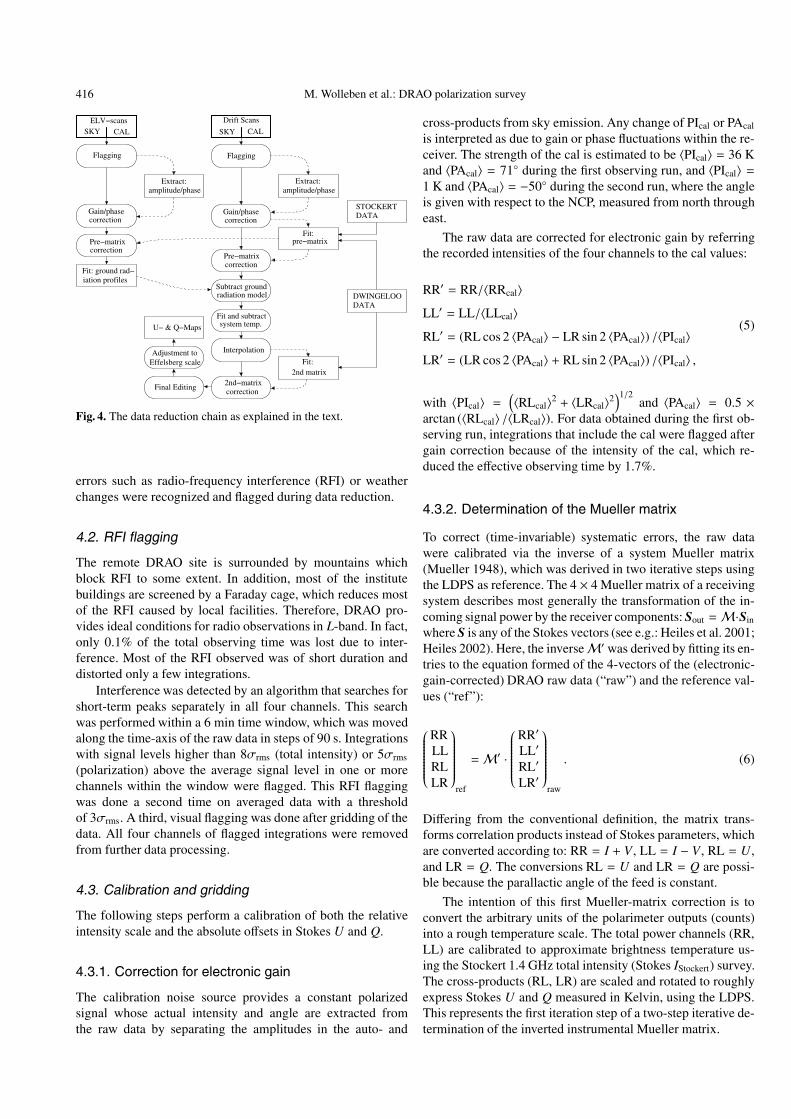
In the following we summarize the data processing steps ap-plied to the raw data. A flow chart of the reduction chain isdisplayed in Fig. 4. Here, we neglect the total power data (RR,LL), which are only used for the correction of main beam in-strumental polarization during data reduction and are not in-tended to be published.

4.1. General overall strategy

For the absolute calibration of the Stokes U and Q data the fol-lowing calibration scheme was applied. The LDPS at 1.4 GHzprovided 1666 absolutely calibrated pointings observed northof 0◦ declination. We used a digitized version of these data,kindly provided by T. Spoelstra, as reference values for the de-termination of the system parameters of our instrument and thedetermination of zero levels in U and Q. While surveying thesky, 946 of these pointings (referred to as congruent pointingsif their centers match within a radius of 15′) were observed inthe course of the drift scans and used for the calibration. In thisway we effectively corrected our observations north of 0◦ dec-lination for ground radiation. For the extrapolation of the zerolevels below 0◦ declination, profiles of ground radiation weremeasured. In a final calibration step, the main-beam bright-ness temperature scale in U and Q of the DRAO survey wasrefined by comparison with data taken from the EMLS (seeSect. 4.3.7).

Serious time-variable errors were found to arise from fluc-tuations of Tsys. These could be corrected by comparing driftscans with neighboring scans and thus separating instrumen-tal variations from variations of the sky brightness temperaturein U and Q. Fluctuations of the electronic gain, most likelycaused by the LNAs, were corrected using the cal. Solar in-terference and ionospheric Faraday rotation could largely beavoided by not observing during day-time. Other time-variable


DATASTOCKERT

U− & Q−Maps

Effelsberg scaleAdjustment to

Flagging

CALSKYELV−scans

SKY CAL

Flagging

Gain/phasecorrection

Pre−matrixcorrection

Fit: ground rad−iation profiles

Extract: Extract:

Fit:pre−matrix

Gain/phasecorrection

correctionPre−matrix

radiation modelSubtract ground

system temp.Fit and subtract

Interpolation

2nd matrixFit:

correction2nd−matrix

Final Editing

Drift Scans

amplitude/phaseamplitude/phase

DATADWINGELOO

Fig. 4. The data reduction chain as explained in the text.

errors such as radio-frequency interference (RFI) or weatherchanges were recognized and flagged during data reduction.

4.2. RFI flagging

The remote DRAO site is surrounded by mountains whichblock RFI to some extent. In addition, most of the institutebuildings are screened by a Faraday cage, which reduces mostof the RFI caused by local facilities. Therefore, DRAO pro-vides ideal conditions for radio observations in L-band. In fact,only 0.1% of the total observing time was lost due to inter-ference. Most of the RFI observed was of short duration anddistorted only a few integrations.

Interference was detected by an algorithm that searches forshort-term peaks separately in all four channels. This searchwas performed within a 6 min time window, which was movedalong the time-axis of the raw data in steps of 90 s. Integrationswith signal levels higher than 8σrms (total intensity) or 5σrms

(polarization) above the average signal level in one or morechannels within the window were flagged. This RFI flaggingwas done a second time on averaged data with a thresholdof 3σrms. A third, visual flagging was done after gridding of thedata. All four channels of flagged integrations were removedfrom further data processing.

4.3. Calibration and gridding

The following steps perform a calibration of both the relativeintensity scale and the absolute offsets in Stokes U and Q.

4.3.1. Correction for electronic gain

The calibration noise source provides a constant polarizedsignal whose actual intensity and angle are extracted fromthe raw data by separating the amplitudes in the auto- and

cross-products from sky emission. Any change of PIcal or PAcal

is interpreted as due to gain or phase fluctuations within the re-ceiver. The strength of the cal is estimated to be 〈PIcal〉 = 36 Kand 〈PAcal〉 = 71◦ during the first observing run, and 〈PIcal〉 =1 K and 〈PAcal〉 = −50◦ during the second run, where the angleis given with respect to the NCP, measured from north througheast.

The raw data are corrected for electronic gain by referringthe recorded intensities of the four channels to the cal values:

RR′ = RR/〈RRcal〉LL′ = LL/〈LLcal〉RL′ = (RL cos 2 〈PAcal〉 − LR sin 2 〈PAcal〉) /〈PIcal〉LR′ = (LR cos 2 〈PAcal〉 + RL sin 2 〈PAcal〉) /〈PIcal〉 ,

(5)

with 〈PIcal〉 =(〈RLcal〉2 + 〈LRcal〉2

)1/2and 〈PAcal〉 = 0.5 ×

arctan (〈RLcal〉 /〈LRcal〉). For data obtained during the first ob-serving run, integrations that include the cal were flagged aftergain correction because of the intensity of the cal, which re-duced the effective observing time by 1.7%.

4.3.2. Determination of the Mueller matrix

To correct (time-invariable) systematic errors, the raw datawere calibrated via the inverse of a system Mueller matrix(Mueller 1948), which was derived in two iterative steps usingthe LDPS as reference. The 4 × 4 Mueller matrix of a receivingsystem describes most generally the transformation of the in-coming signal power by the receiver components: Sout =M·Sin

where S is any of the Stokes vectors (see e.g.: Heiles et al. 2001;Heiles 2002). Here, the inverseM′ was derived by fitting its en-tries to the equation formed of the 4-vectors of the (electronic-gain-corrected) DRAO raw data (“raw”) and the reference val-ues (“ref”):

⎛⎜⎜⎜⎜⎜⎜⎜⎜⎜⎜⎜⎜⎝

RRLLRLLR

⎞⎟⎟⎟⎟⎟⎟⎟⎟⎟⎟⎟⎟⎠ref

=M′ ·

⎛⎜⎜⎜⎜⎜⎜⎜⎜⎜⎜⎜⎜⎝

RR′

LL′

RL′

LR′

⎞⎟⎟⎟⎟⎟⎟⎟⎟⎟⎟⎟⎟⎠raw

. (6)

Differing from the conventional definition, the matrix trans-forms correlation products instead of Stokes parameters, whichare converted according to: RR = I + V , LL = I − V , RL = U,and LR = Q. The conversions RL = U and LR = Q are possi-ble because the parallactic angle of the feed is constant.

The intention of this first Mueller-matrix correction is toconvert the arbitrary units of the polarimeter outputs (counts)into a rough temperature scale. The total power channels (RR,LL) are calibrated to approximate brightness temperature us-ing the Stockert 1.4 GHz total intensity (Stokes IStockert) survey.The cross-products (RL, LR) are scaled and rotated to roughlyexpress Stokes U and Q measured in Kelvin, using the LDPS.This represents the first iteration step of a two-step iterative de-termination of the inverted instrumental Mueller matrix.


The reference values for the computation of the pre-calibration matrix are given by:

RRref = (0.5 × 1.55 (IStockert − 2.8 K)) + 2.8 K

LLref = (0.5 × 1.55 (IStockert − 2.8 K)) + 2.8 K

RLref = ULDPS

LRref = QLDPS,

(7)

which includes the transformation of full-beam into main-beambrightness temperature of the Stockert survey with a scalingfactor of 1.55 and the correction for extragalactic backgroundemission of 2.8 K (Reich & Reich 1988), which is subtractedand subsequently added. Stokes V is assumed zero.

The fitting of the pre-calibration matrix proceeds us-ing Eq. (6). For each point, Stockert data supply RRref =

LLref. The Dwingeloo telescope provides RLref and LRref. TheDRAO 26-m telescope provides all matrix elements on the righthand side of Eq. (6), allowingM′1 to be determined. Hence, ifthe total number of pointings is N, the resulting set of equationswith n = 1, 2, . . . ,N for RR and LL reads:

RRref,n = m11

(RR′sky,n + RR′off,n

)

LLref,n = m22

(LL′sky,n + LL′off,n

).

(8)

For RL and LR it is:

RLref,n = m33

(RL′sky,n + RL′off,n

)+ m34

(LR′sky,n + LR′off,n

)

LRref,n = m43

(RL′sky,n + RL′off,n

)+ m44

(LR′sky,n + LR′off,n

).

(9)

At this point the raw data still contain time-variable off-sets (“off”) in addition to the sky values (“sky”). Therefore,the matrix entries m11, m22, m33, m44, m34 and m43 of the ma-trixM′1 can only be fitted iteratively by approximation of theseoffsets as done in the following algorithm:

1. the DRAO raw data for congruent pointings are correctedfor electronic gain;

2. the initial matrixM′1 is set to be the unit matrix;3. the DRAO raw data are corrected by multiplication

withM′1 according to Eq. (6);4. ground radiation and system temperature drifts are ap-

proximately removed by subtracting a linear baseline fittedthrough all congruent pointings at equal declination from 0h

to 24h right ascension;5. the fit-error is given as the sum of the squared differences

between corrected DRAO data and the reference values;6. matrix entries of M′1 are either randomly altered and the

iteration continues at point three or the iteration is stoppedif the minimization of the fit-error is achieved.

This way, pre-calibration matrices have been determined foreach observing month, using about 100 congruent point-ings per month. These monthly matrices were checked fortime-variability and then averaged. No systematic variation ofthe matrix entries with time were found bigger than the fittingerrors.

30o

50o

70o

90o

70o

50o

Elevation

-3.8

-3.6

-3.4

Stokes Q

30o

50o

70o

90o

70o

50o

Elevation

2.5

3

3.5

4

4.5

TB (

K)

Stokes U

NSNS

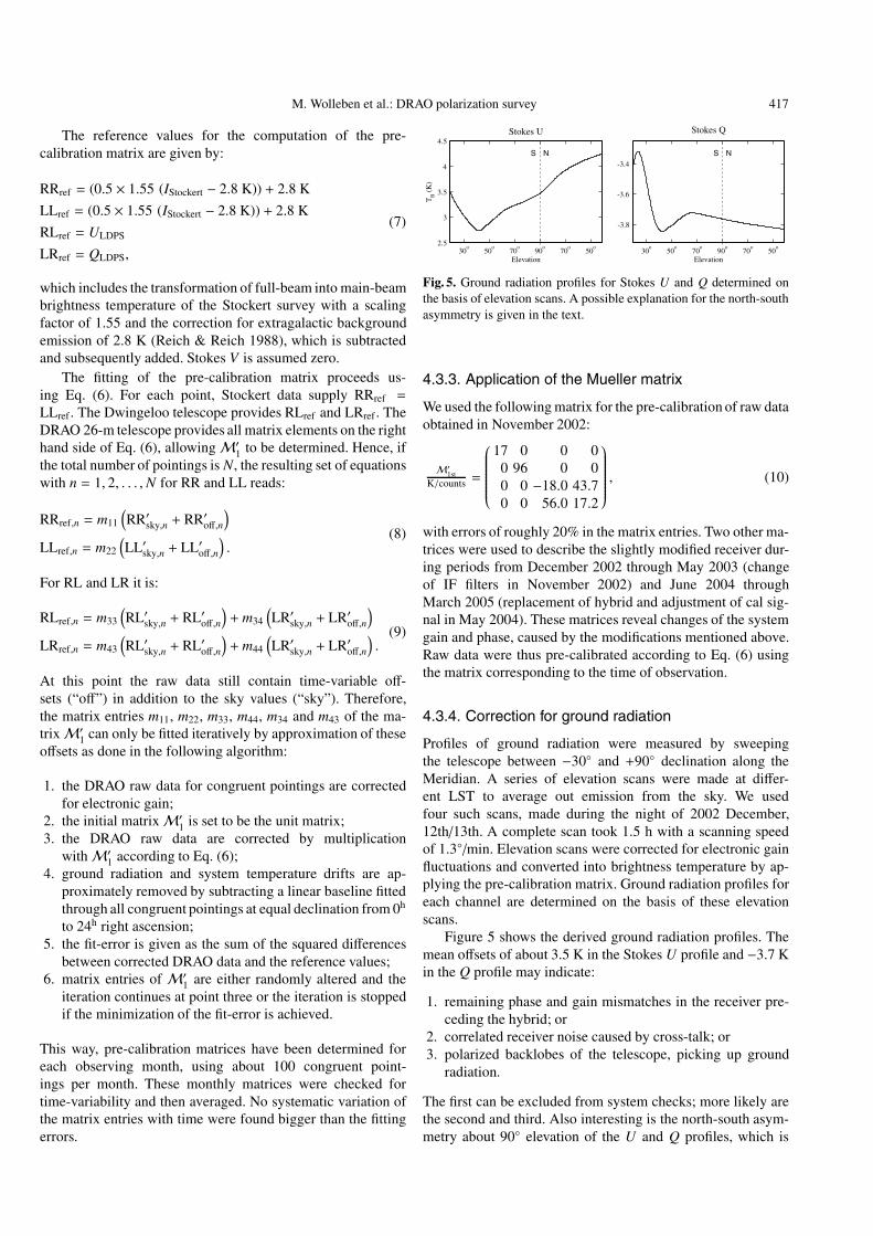
Fig. 5. Ground radiation profiles for Stokes U and Q determined onthe basis of elevation scans. A possible explanation for the north-southasymmetry is given in the text.

4.3.3. Application of the Mueller matrix

We used the following matrix for the pre-calibration of raw dataobtained in November 2002:

M′1stK/counts =

⎛⎜⎜⎜⎜⎜⎜⎜⎜⎜⎜⎜⎜⎝

17 0 0 00 96 0 00 0 −18.0 43.70 0 56.0 17.2

⎞⎟⎟⎟⎟⎟⎟⎟⎟⎟⎟⎟⎟⎠, (10)

with errors of roughly 20% in the matrix entries. Two other ma-trices were used to describe the slightly modified receiver dur-ing periods from December 2002 through May 2003 (changeof IF filters in November 2002) and June 2004 throughMarch 2005 (replacement of hybrid and adjustment of cal sig-nal in May 2004). These matrices reveal changes of the systemgain and phase, caused by the modifications mentioned above.Raw data were thus pre-calibrated according to Eq. (6) usingthe matrix corresponding to the time of observation.

4.3.4. Correction for ground radiation

Profiles of ground radiation were measured by sweepingthe telescope between −30◦ and +90◦ declination along theMeridian. A series of elevation scans were made at differ-ent LST to average out emission from the sky. We usedfour such scans, made during the night of 2002 December,12th/13th. A complete scan took 1.5 h with a scanning speedof 1.3◦/min. Elevation scans were corrected for electronic gainfluctuations and converted into brightness temperature by ap-plying the pre-calibration matrix. Ground radiation profiles foreach channel are determined on the basis of these elevationscans.

Figure 5 shows the derived ground radiation profiles. Themean offsets of about 3.5 K in the Stokes U profile and −3.7 Kin the Q profile may indicate:

1. remaining phase and gain mismatches in the receiver pre-ceding the hybrid; or

2. correlated receiver noise caused by cross-talk; or3. polarized backlobes of the telescope, picking up ground

radiation.

The first can be excluded from system checks; more likely arethe second and third. Also interesting is the north-south asym-metry about 90◦ elevation of the U and Q profiles, which is


probably due to the multipole structure of the response patternof the telescope to unpolarized radiation. The response patternof the DRAO 25.6-m telescope in total power was measured byHiggs & Tapping (2000) and shows sidelobe structure to radiias far as 45◦ off the main beam at a level above −49 dB. Theseare mostly caused by aperture blockage due to the three supportstruts and the receiver box. Irregularities of the antenna surfacecomplicate the sidelobe structure.

Subtraction of ground radiation from the raw data isstraightforward. The ground offsets for each declination (be-tween −29◦ and +90◦ declination) and channel are taken fromthe profiles. These offsets are then subtracted from the driftscans. This way, the declination-dependent component is re-moved and only the time-variable components of ground radi-ation and system temperature are left; these are corrected later(see Sect. 4.3.6). The remaining uncertainties of this procedureare around 50 mK or less, according to the variations betweenindividual elevation scans at positions where polarized emis-sion from the sky is low.

4.3.5. Solar interference and ionospheric Faradayrotation

The data were visually inspected by comparing drift scanswith neighboring scans to identify high levels of ionosphericFaraday rotation or solar interference. Only some of theday-time data, observed shortly before sunset and after sun-rise, show apparent solar interference and needed to be flagged.No indication was found for ionospheric Faraday rotationat night.

4.3.6. System temperature fluctuations

Data reduction was made more difficult by fluctuations of sys-tem temperature, Tsys. Fluctuations of the order of several partsin 1000 (a few hundred mK in ∼100 K) were subsequentlyfound to have occurred throughout both observing periods.Fluctuations in the RHCP and LHCP channels were not corre-lated, and there was no apparent correlation of the fluctuationsof Tsys with time of year, temperature, rain, or other variables.Over periods of months we found the amplitude of these vari-ations to be several Kelvin. In subsequent observing nights thebaselevels of drift scans differed by several hundreds of mK (af-ter correction for ground radiation). Such fluctuations occurredon time scales from hours to months. The origin of these fluc-tuations is unknown.

The Tsys-fluctuations must be corrected while large-scalesky emission in the data should be preserved to obtain abso-lutely calibrated maps. However, variations of the system tem-perature cannot easily be distinguished from real sky emission.An algorithm was applied that effectively separates randomfluctuations from systematic sky emission (see Appendix A).The remaining errors are of the order of 50 mK at maximum asindicated by simulations5.

5 For this, the algorithm was applied to artificial Stokes Uand Q maps with simulated noise and Tsys-fluctuations added to them.

4.3.7. Refinement of the Mueller matrix

A more accurate scaling and rotation of the RL and LR scalesand a correction for main beam instrumental polarization wereachieved by the second calibration. No further corrections ofthe total power data were made as the intention was the cali-bration of polarization. Instead of iterative fitting, here least-square fitting can be applied because the raw data are nowcorrected for ground radiation offsets. The reference points areagain taken from the LDPS.

A single calibration matrix is determined for the whole dataset. The following correction matrix was derived:

M′2nd =

⎛⎜⎜⎜⎜⎜⎜⎜⎜⎜⎜⎜⎜⎝

1 0 0 00 1 0 0

0.001 0.0001 1.125 −0.013−0.009 −0.011 0.051 1.240

⎞⎟⎟⎟⎟⎟⎟⎟⎟⎟⎟⎟⎟⎠, (11)

with errors of around ±0.01 in the matrix entries. Raw datawere corrected according to Eq. (6). The second calibrationmatrix mainly corrected scaling errors that were introducedby the separation of Tsys-fluctuations. Instrumental polariza-tion within the main-beam (cross-talk) is given by RLinst =

m2nd,31 ·RR+m2nd,32 ·LL and LRinst = m2nd,41 ·RR+m2nd,42 ·LLand hence amounts to 0.1% in Stokes U and −2.0% in Q.

4.3.8. Gridding and interpolation

Integrations were averaged and binned into a grid of equatorialcoordinates with 15′ cell size, which is less then the telescope’sHPBW/2 required for full Nyquist sampling. No weightingscheme was used; measured values were uniformly weightedand averaged across the cell.

An interpolation between scans needs to be applied. In con-trast to “uniform” undersampling, the DRAO survey is fullysampled along right ascension and undersampled in declina-tion. Considering this specific sampling problem an interpo-lation routine working in the Fourier domain was applied.The drifts scans were Fourier transformed, using the DFT6-algorithm of AIPS++. Unobserved declinations were then filledby linear interpolation in the Fourier space. The interpolatedscans were then reverse transformed into the image plane.

4.3.9. Temperature scale refinement with the EMLS

Brightness temperatures from the DRAO survey were com-pared with the EMLS over an area of 1800 square degrees ofsky. Two preliminary maps from the EMLS were used: a 35◦ ×35◦ map towards Cassiopeia-A and a 40◦ × 16◦ map coveringthe Taurus-Auriga-Perseus molecular clouds.

As the EMLS lacks large-scale emission a direct compari-son with the DRAO survey is not meaningful. Therefore, miss-ing large-scale structures were approximated by polynomials.The coefficients of these polynomials and the scaling factor ofthe DRAO temperature scale were fitted to the Effelsberg dataover the entire region, with the difference between EMLS andDRAO survey to be minimized. Figure 6 shows four constantdeclination scans, two through each comparison region.

6 Discrete Fourier Transformation.


55 60 65 70 75-300

-200

-100

0

100

200

Stok

es-U

(m

K)

Taurus Field

320 330 340 350 360 370 380

-100

0

100

200

300

400Cas-A Field

60 65 70 75Right Ascension

-300

-200

-100

0

100

200

Stok

es-Q

(m

K)

320 330 340 350Right Ascension

-100

0

100

200=δ o29.75

= 31.5 oδ = 68.5 oδ

= 65.5 oδ

Fig. 6. Four scans through the two test regions used to establishthe calibration of the survey relative to EMLS observations (thinsolid lines), two from the Taurus complex (left panels) and twofrom the Cassiopeia-A region (right panels). DRAO survey data aredrawn as thick solid lines. The large-scale emission missing from theEMLS data are shown as polynomials (whose characteristics were de-termined by an iterative technique and added to the EMLS data shownin this figure – see text) and are drawn as dashed lines. The declina-tions of the scans are indicated.

The calibration of the EMLS is based on standard cali-bration sources (Uyaniker et al. 1998), particularly the well-established value for the polarized flux density of 3C 286, andcan thus be assumed to be more accurate than the LDPS cal-ibration. The LDPS is not sufficiently sensitive to allow cali-bration by compact sources, but relies on a set of calibrationpoints (α = 57.◦0, δ = 64.◦0 and α = 240.◦0, δ = 23.◦0) onthe sky where polarized intensities were determined earlier atCambridge with a larger beam (Bingham 1966). Frequent ob-servations of these calibration points gave a high internal con-sistency to the LDPS, but the accuracy of the scale is not com-parable with that achievable at the Effelsberg telescope today.

5. Accuracy and errors

The theoretical rms noise for the correlation receiver used here,with a bandwidth of 12 MHz, and an integration time of 60 s,calculates to 3 mK (valid for Stokes U and Q). In the follow-ing we summarize the measured rms noise and the systematicerrors of this survey.

5.1. RMS estimation

Taking the NCP measurements (Sect. 3.1), the deviation froma circle in the U-Q plane gives the resulting rms noise ofthe DRAO survey. This is, for an integration time of 60 s,12 mK rms in Stokes U and Q taking only night-time data intoaccount, and ∼35 mK including day-time data.

Figure 7 shows the correlation of the final data with thereference values, prior to adjusting the DRAO intensities tothe EMLS. The correlation coefficients are rU = 0.89 and

-500 -250 0 250 500Dwingeloo - U (mK)

-500

-250

0

250

500

DR

AO

(m

K)

-500 -250 0 250 500Dwingeloo - Q (mK)

Fig. 7. Correlation of Stokes U (left panel) and Q (right panel) valuesfrom the DRAO survey with the Dwingeloo survey before adjustingthe temperatures to the Effelsberg scale.

Table 2. Survey specifications.

Integration time per 15′ in RA 60 s

Observing period November 2002–May 2003

June 2004–March 2005

Final rms-noise 12 mK

Systematic errors <∼50 mK

Declination range −29◦ to +90◦

Fully sampled area 41.7%

rQ = 0.86. Numerical calculations7 show that, to reproducethese correlation coefficients, the rms noise in the DRAO datamust be 12 mK in Stokes U, and 33 mK in Q. The differ-ence may reflect an error in the Dwingeloo data higher thanthe quoted error of 60 mK. We note that, based on these cal-culations and the LDPS data, the best achievable correlationbetween the two data sets is rU = rQ = 0.90.

5.2. Resulting error

Based on the NCP measurement and the correlation coeffi-cients the final rms noise in Stokes U and Q is 12 mK, whichis 9 mK higher than the theoretical rms noise. Systematicerrors are introduced during the separation of sky emissionand Tsys-fluctuations. In case of intense polarized structures,which are elongated along right ascension, this error may be<∼50 mK, depending on the shape, intensity, and coverage ofthe structure. At declinations ≤0◦ a systematic baselevel errorof <∼50 mK may be caused by uncertainties in the ground pro-files, which should be highest at the lowest declination.

5.3. Instrumental artifacts

A correction for instrumental polarization caused by sidelobesis not intended for this survey. This requires fully sampled totalintensity maps and precise measurements of the response pat-tern of the DRAO telescope in polarization. Some instrumentalpolarization effects can be seen around intense compact sourcesin Figs. 8 and 9 (e.g. Taurus-A at RA = 5h35m, Dec = −5◦30′

7 These assume the quoted error of 60 mK of the LDPS, and a nor-mal distribution of U and Q around zero with a FWHM of 120 mK.


��

��

��

��

��

��

��

TBMB (mK)

12hh18 h16 h14h2024h 22h

Right Ascension (J2000)

Dec

linat

ion

(J20

00)

Stokes U

��

��

��

��

��

��

��

��

TBMB (mK)

12hh18 h16 h14h2024h 22h


Dec

linat

ion

(J20

00)

Stokes Q

Fig. 8. Stokes U (top) and Q (bottom) in the right ascension interval from 12h to 24h in equatorial coordinates.

in Fig. 9). Instrumental effects are also seen around the intenseemission from the Galactic plane in directions towards the in-ner Galaxy (from RA = 17h38m, Dec = −29◦ to RA = 19h40m,

Dec = 20◦) seen especially in the U image of Fig. 8. These in-strumental effects do not extend beyond a few degrees. Someinstrumental effects have the appearance of scanning artifacts,


��

��

��

��

��

��

��

TBMB (mK)

12h 10h 8h 6h 4h 2 h 0h


Dec

linat

ion

(J20

00)

Stokes U

��

��

��

��

��

��

��

��

TBMB (mK)

12h 10h 8h 6h 4h 2 h 0h


Dec

linat

ion

(J20

00)

Stokes Q

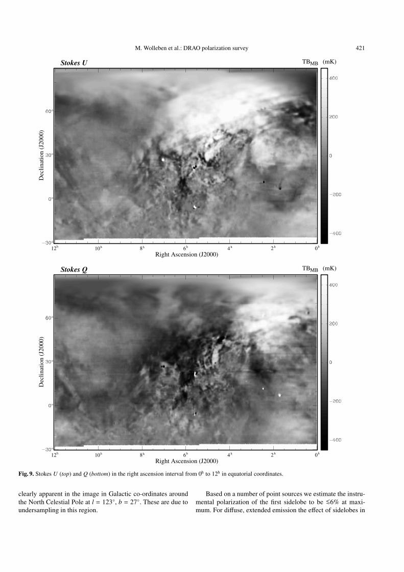
Fig. 9. Stokes U (top) and Q (bottom) in the right ascension interval from 0h to 12h in equatorial coordinates.

clearly apparent in the image in Galactic co-ordinates aroundthe North Celestial Pole at l = 123◦, b = 27◦. These are due toundersampling in this region.

Based on a number of point sources we estimate the instru-mental polarization of the first sidelobe to be <∼6% at maxi-mum. For diffuse, extended emission the effect of sidelobes in


Fig. 10. Polarized intensity in Galactic coordinates. The projection center is at l = b = 0◦. The co-ordinate grid is in steps of 60◦ in Galacticlongitude and 30◦ in Galactic latitude.

most likely negligible because their contributions over a largearea around the main beam average close to zero.

6. Final maps and data availability

The final maps in Stokes U and Q are displayed in Figs. 8 and 9in equatorial co-ordinates in the rectangular projection in whichthe data processing and gridding were done. Figure 10 showspolarized intensity in Galactic co-ordinates in Aitoff projection.In this section we will comment on the most prominent astro-nomical results. Detailed interpretation of the newly discoveredfeatures must await a forthcoming paper.

The most intensely polarized features of the Northern skyare the North Polar Spur, at Galactic latitudes higher than 25◦,extending from longitude 300◦ to 40◦, and the Fan Region,of extent 60◦ by 30◦, centred on l = 140◦, b = 5◦. Thesefeatures were readily apparent in older data (e.g. Brouw &Spoelstra 1976). Some large nearby H ii regions can be seenas depolarization zones. Particularly obvious are Sharpless 27(l = 6◦, b = 23◦), distance 170 pc, and Sharpless 220 (l = 163◦,b = −15◦), distance 400 pc. Such depolarization effects can beused to establish a minimum distance to the polarized emissionregions.

The North Polar Spur coincides with a bright emission fea-ture seen in total intensity in many Galactic surveys. It is gen-erally considered to be a supernova remnant (SNR), generatedby the explosion of a member of the Sco-Cen association ata distance of about 150 pc (Berkhuijsen 1971). In Fig. 11 weshow the southern part of this spur.

The Fan Region, in contrast, has no obvious counterpartin total intensity. A polarization map is shown in Fig. 11.Earlier investigators considered this polarized emission to orig-inate at distances under 500 pc (Wilkinson & Smith 1974;

Spoelstra 1984). H ii regions seen in the same direction did notappear to depolarize the emission from the Fan Region, andthe polarized emission was therefore considered to be closerthan the H ii regions, whose distances were known. With ournew data, which has greatly improved sampling and sensitiv-ity, we can re-examine this conclusion. We have detected def-inite depolarization by a number of H ii regions seen againstthe Fan Region (Wolleben 2005). On the basis of this new ev-idence we conclude that the polarized emission from the FanRegion originates over a range of distances, extending from500 pc to a few kpc, the latter distance corresponding to thedistance of the Perseus arm. Over much of the Fan Region theelectric vectors are perpendicular to the Galactic plane, indi-cating that the magnetic field is aligned with the plane. Thefractional polarization in this region is up to 50%, not muchlower than the theoretical maximum of 70%, indicating thatthere must be a very regular magnetic field structure and verylittle depolarization along a long line of sight, extending rightthrough the Perseus arm.

A new result that is apparent in our data is a depolariza-tion region that extends between latitudes +30◦ and −30◦, fromlongitude about 65◦ towards longitude zero. Our superior cov-erage as well as sensitivity and the representation of the datain grayscale, as in Fig. 10, reveals the small-scale structure inthis region. The typical feature size in this region is no morethan a few degrees. Earlier surveys with their sampling of ordertwo degrees could not show this region adequately. The depo-larization must arise in a very nearby magneto-ionic region: theemission from the North Polar Spur is depolarized, and the dis-tance to the Spur is no more than 150 pc. Particularly strikingare the sharp upper and lower boundaries of this depolarizationregion.


Fig. 11. The two maps of polarized intensity, with E-vectors of the polarized emission overlayed, show in greater detail part of the Fan-region(left panel) and the southern extension of the North-Polar Spur (right panel). In both maps depolarization caused by local H ii-regions isapparent (NGC 1499: from l = 145◦ to 170◦, b <∼ −10◦; and Sharpless 27: roughly 10◦ in diameter, centered at l = 6◦ and b = 23◦). Thesynchrotron emission of the North-Polar spur seems to be depolarized at b <∼ 25◦ (from l = 30◦ to 40◦). In both maps contours of polarizedintensity run from 0 mK to 800 mK in steps of 100 mK. Vectors are shown on a grid of 1.25◦.

Examination of polarization angles at Galactic latitudesabove 70◦, both north and south, shows systematic changeswith position and a remarkable symmetry of polarized inten-sity. Fractional polarization reaches values of 50% (northernpole) and 30% (southern pole). These results suggest that theSun is located inside a synchrotron emitting shell with the mag-netic field parallel to the Galactic plane.

The 1.41 GHz polarization data presented here areavailable in Galactic or equatorial coordinates via the follow-ing web-pages: http://www.mpifr-bonn.mpg.de/div/konti/26msurveyor http://www.drao.nrc.ca/26msurvey.Alternatively, the reader may contact M.W. at [email protected]. Ungridded data may be madeavailable on request in form of tables.

7. Summary

We have presented a new survey of linear polarization ofthe northern sky, obtained using the DRAO 25.6-m telescopeat 1.4 GHz. Observations were made by drift scanning the skyto keep ground radiation as constant as possible, which allowsan absolute calibration of the Stokes U and Q maps. A fullysampled area of 41.7% has been observed. Although a com-plete coverage of the northern sky could not be achieved, thisdata base provides about 200 times more data points than dataso far available and sensitivity 5 times better than previous data.The new survey reveals previously unknown structures and ob-jects in polarization and provides valuable information for thederivation of foreground templates of polarized emission re-quired for CMB experiments.

Acknowledgements. We thank A. Gray and E. Fürst for critical read-ing of the manuscript. We are also grateful to J. Bastien for maintain-ing the telescope and J. Galt for his support during early stages of thisproject. The analog polarimeter has been improved by K. Grypstra.

Remote observing from the MPIfR would not have been possible with-out D. Del Rizzo and A. Hoffmann. We thank T. Spoelstra for provid-ing the Leiden/Dwingeloo polarization surveys in digital form. Wealso thank the anonymous referee for many valuable comments whichhave led to improvements in the paper. This project forms part of theInternational Galactic Plane Survey. Within Canada, the project is sup-ported by the Natural Sciences and Engineering Research Council.The Dominion Radio Astrophysical Observatory is operated as a na-tional Facility by the National Research Council Canada.

Appendix A: Algorithm for correctionof Tsys-fluctuations

This algorithm compares each drift scan pairwise withits neighboring scans. The basic assumption is made thatTsys-fluctuations are random on time-scales of weeks, whichmeans that fluctuations observed at the same declination butweeks apart are assumed to be uncorrelated. Therefore neigh-boring drift scans with slightly different declinations were ob-served weeks apart so that system temperature fluctuationsmight differ, but not the large-scale structure contained inthese scans. The declination range from which neighboringscans are selected is adjustable in the program as described inthe following.

The following performs an iterative separation of randomand systematic structures in the drift scans. Let m be an indexnumbering all observed drift scans. The following loop is ap-plied until m has reached the total number of scans:

1. To the drift scan with index m all neighboring scans nwithin ±δ◦ in declination are assorted. Values for δ be-tween 3 and 40 were found to be useful here. Thesenumbers reflect the sampling and should decrease withmore complete coverage or larger number of drift scans,respectively.


2. Each pair of drift scans (m, n) is convolved with a Gaussian.The width of the Gaussian is σ times the separation indeclination ∆dm,n = |dm − dn| of the two drift scans. Thisremoves spatial structures smaller than σ × ∆dm,n. Valuesfor σ between 4 and 100 are useful here.

3. The weight wm,n = |δ − ∆dm,n| is introduced.4. The difference of each pair of drift scans ∆Tm,n is cal-

culated. The sum of these differences multiplied with theweight wm,n is then subtracted from the mth drift scan:T ′m = Tm − ∑n wm,n × ∆Tm,n with T denoting brightnesstemperature.

5. Index m is increased by one and the loop restarted until mreaches the number of scans.

This algorithm was applied several times with different param-eters until a satisfactory separation of sky emission and sys-tem temperature was achieved. The following parameters wereused: loops 1 to 4: δ = 40, σ = 100; loop 5: δ = 10, σ = 15;loops 6–9: δ = 6, σ = 8; loops 10–11: δ = 3, σ = 4.

References

Anderson, M. D., Landecker, T. L., Routledge, D., & Vaneldik, J. F.1991, Radio Science, 26, 353

Baccigalupi, C., Burigana, C., Perrotta, F., et al. 2001, A&A, 372, 8Berkhuijsen, E. M. 1971, A&A, 14, 359Berkhuijsen, E. M. 1975, A&A, 40, 311Berkhuijsen, E. M., & Brouw, W. N. 1963, Bull. Astron. Inst.

Netherlands, 17, 185Bingham, R. G. 1966, MNRAS, 134, 327Brouw, W. N., & Spoelstra, T. A. T. 1976, A&AS, 26, 129Burigana, C., & La Porta, L. 2002, in Astrophysical Polarized

Backgrounds, ed. S. Cecchini, S. Cortiglioni, R. Sault, & C. Sbarra(NY: Melville), AIP Conf. Proc., 609, 54

Gaensler, B. M., Dickey, J. M., McClure-Griffiths, N. M., et al. 2001,ApJ, 549, 959

Gibbins, C. J. 1986, Radio Science, 21, 949Gray, A. D., Landecker, T. L., Dewdney, P. E., & Taylor, A. R. 1998,

Nature, 393, 660Gray, A. D., Landecker, T. L., Dewdney, P. E., et al. 1999, ApJ, 514,

221Heiles, C. 2002, in ASP Conf. Ser., ed. S. Stanimirovic, D. Altschuler,

P. Goldsmith, & C. Salter, 278, 131Heiles, C., Perillat, P., Nolan, M., et al. 2001, PASP, 113, 1274Higgs, L. A., & Tapping, K. F. 2000, AJ, 120, 2471

Knee, L. B. G. 1997, DRAO Internal ReportMathewson, D. S., Broten, N. W., & Cole, D. J. 1965, Australian J.

Phys., 18, 665Mathewson, D. S., Broten, N. W., & Cole, D. J. 1966, Australian J.

Phys., 19, 93McMullin, J. P., Golap, K., & Myers, S. T. 2004, in ASP Conf. Ser.,

ed. F. Ochsenbein, M. G. Allen, & D. Egret, 314, 468Mueller, H. 1948, J. Opt. Soc. Am., 38, 661Muller, C. A., Berkhuijsen, E. M., Brouw, W. N., & Tinbergen, J.

1963, Nature, 200, 155Ng, T., Landecker, T. L., Cazzolato, F., et al. 2005, Radio Science,

in pressReich, W. 1982, A&AS, 48, 219Reich, P., & Reich, W. 1986, A&AS, 63, 205Reich, P., & Reich, W. 1988, A&AS, 74, 7Reich, W., & Wielebinski, R. 2000, in Radio Polarization: a New

Probe of the Galaxy, Proceedings of a Workshop held at Universitéde Mentréal, ed. T. L. Landecker

Reich, W., Fürst, E., Haslam, C. G. T., Steffen, P., & Reif, K. 1984,A&AS, 58, 197

Reich, W., Fürst, E., Reich, P., et al. 2004, in The MagnetizedInterstellar Medium, ed. B. Uyaniker, W. Reich, & R. Wielebinski,45

Spoelstra, T. A. T. 1972, A&AS, 5, 205Spoelstra, T. A. T. 1984, A&A, 135, 238Taylor, A. R., Gibson, S. J., Peracaula, M., et al. 2003, AJ, 125, 3145Testori, J. C., Reich, P., & Reich, W. 2004, in The Magnetized

Interstellar Medium, ed. B. Uyaniker, W. Reich, & R. Wielebinski,57

Uyaniker, B., Fürst, E., Reich, W., Reich, P., & Wielebinski, R. 1998,A&AS, 132, 401

Uyaniker, B., Fürst, E., Reich, W., Reich, P., & Wielebinski, R. 1999,A&AS, 138, 31

Uyaniker, B., Landecker, T. L., Gray, A. D., & Kothes, R. 2003, ApJ,585, 785

Westerhout, G., Seeger, C. L., Brouw, W. N., & Tinbergen, J. 1962,Bull. Astron. Inst. Netherlands, 16, 187

Wielebinski, R., & Shakeshaft, J. R. 1964, MNRAS, 128, 19Wielebinski, R., Shakeshaft, J. R., & Pauliny-Toth, I. I. K. 1962, The

Observatory, 82, 158Wilkinson, A., & Smith, F. G. 1974, MNRAS, 167, 593Willis, A. G. 2002, in Astronomical Data Analysis Software and

Systems XI, ASP Conf. Ser., 281, 83Wohlleben, R., Mattes, H., & Lochner, O. 1972, Electronics Letters,

8, 474Wolleben, M. 2005, Ph.D. Thesis, Universität Bonn, Germany

An absolutely calibrated survey of polarized emission from the northern sky at 1.4 GHz

Documents

Transcript of An absolutely calibrated survey of polarized emission from the northern sky at 1.4 GHz