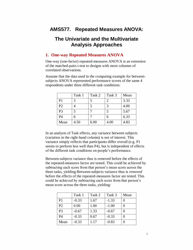
1

AMS577. Repeated Measures ANOVA:

The Univariate and the Multivariate Analysis Approaches

1. One-way Repeated Measures ANOVA

One-way (one-factor) repeated-measures ANOVA is an extension

of the matched-pairs t-test to designs with more columns of

correlated observations.

Assume that the data used in the computing example for between-

subjects ANOVA represented performance scores of the same 4

respondents under three different task conditions:

Task 1 Task 2 Task 3 Mean

P1 3 5 2 3.33

P2 4 5 3 4.00

P3 5 7 5 5.67

P4 6 7 6 6.33

Mean 4.50 6.00 4.00 4.83

In an analysis of Task effects, any variance between subjects

(variation in the right-hand column) is not of interest. This

variance simply reflects that participants differ overall (e.g. P1

seems to perform less well than P4), but is independent of effects

of the different task conditions on people’s performance.

Between-subjects variance thus is removed before the effects of

the repeated-measures factor are tested. This could be achieved by

subtracting each score from that person’s mean score across the

three tasks, yielding:Between-subjects variance thus is removed

before the effects of the repeated-measures factor are tested. This

could be achieved by subtracting each score from that person’s

mean score across the three tasks, yielding:

Task 1 Task 2 Task 3 Mean

P1 -0.33 1.67 -1.33 0

P2 0.00 1.00 -1.00 0

P3 -0.67 1.33 -0.67 0

P4 -0.33 0.67 -0.33 0

Mean -0.33 1.17 -0.83 0

2

These new scores do not reflect differences between subjects any

more, whereas the differences between task conditions are still

reflected in the column means.

The ANOVA for repeated measurements achieves this by first

partitioning the sums of squares into a “between-subjects”

component (i.e. variation between the row means of the first table)

and a “within-subjects” component (all remaining variation).

The “within-subjects” component is further subdivided in variation

“between treatments” (i.e. between the column means in the

second table) and “error” variation (i.e. within the columns of the

second table).

[The between-subjects component can also be further

subdivided if there are between-subjects factors to be

considered; but this will not concern us for the moment.]

The degrees of freedom are divided into the same

components:

dftotal = kn – 1

dfbetween-ss = n – 1

dfwithin-ss = n(k – 1)

dfbetween-treatments = k – 1

dferror = (n – 1)(k – 1)

Mean squares are derived as usual by dividing sums of

squares with their associated df.

SStotal

SSbetween-subjects SSwithin-subjects

SSbetween-treatments SSerror

3

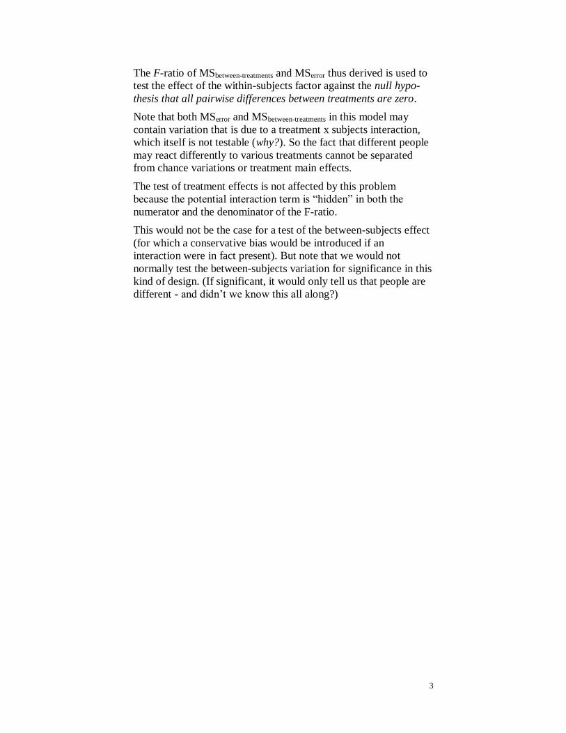
The F-ratio of MSbetween-treatments and MSerror thus derived is used to

test the effect of the within-subjects factor against the null hypo-

thesis that all pairwise differences between treatments are zero.

Note that both MSerror and MSbetween-treatments in this model may

contain variation that is due to a treatment x subjects interaction,

which itself is not testable (why?). So the fact that different people

may react differently to various treatments cannot be separated

from chance variations or treatment main effects.

The test of treatment effects is not affected by this problem

because the potential interaction term is “hidden” in both the

numerator and the denominator of the F-ratio.

This would not be the case for a test of the between-subjects effect

(for which a conservative bias would be introduced if an

interaction were in fact present). But note that we would not

normally test the between-subjects variation for significance in this

kind of design. (If significant, it would only tell us that people are

different - and didn’t we know this all along?)

4

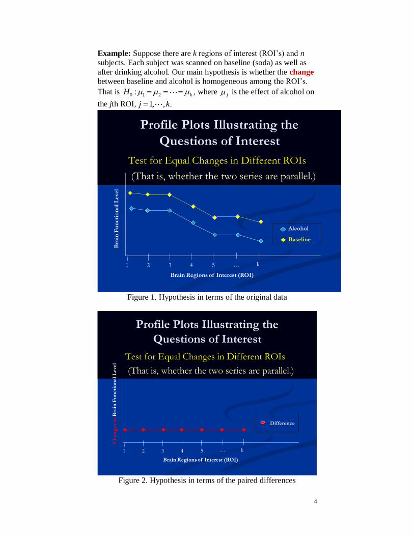
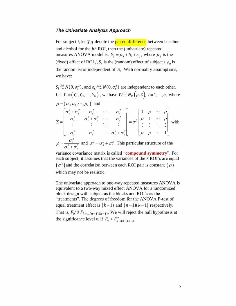
Example: Suppose there are k regions of interest (ROI’s) and n

subjects. Each subject was scanned on baseline (soda) as well as

after drinking alcohol. Our main hypothesis is whether the change

between baseline and alcohol is homogeneous among the ROI’s.

That is 0 1 2: kH , where j is the effect of alcohol on

the jth ROI, 1, , .j k

Profile Plots Illustrating the

Questions of Interest

Test for Equal Changes in Different ROIs

(That is, whether the two series are parallel.)

Alcohol

Baseline

Brain Regions of Interest (ROI)

2 3 4 5 … k

Bra

in F

un

cti

on

al L

eve

l

1

Figure 1. Hypothesis in terms of the original data

Profile Plots Illustrating the

Questions of Interest

Test for Equal Changes in Different ROIs

(That is, whether the two series are parallel.)

Brain Regions of Interest (ROI)

2 3 4 5 … k

Ch

an

ges

in B

rain

Fu

ncti

on

al L

eve

l

1

Difference

Figure 2. Hypothesis in terms of the paired differences

5

The Univariate Analysis Approach

For subject i, let Y ij denote the paired difference between baseline

and alcohol for the jth ROI, then the (univariate) repeated

measures ANOVA model is: ij j i ijY S , where

j is the

(fixed) effect of ROI j, iS is the (random) effect of subject i,ij is

the random error independent of iS . With normality assumptions,

we have:

, and

are independent to each other.

Let '

1 2, , ,i i i ikY Y Y Y , we have , 1, ,i n , where

'

1 2, , , k and

2 2 2 2

2 2 2 2

2

2 2 2 2

1

1

1

s s s

s s s

s s s

with

2

2 2

s

s

and 2 2 2

s . This particular structure of the

variance covariance matrix is called “compound symmetry”. For

each subject, it assumes that the variances of the k ROI’s are equal

2 and the correlation between each ROI pair is constant ,

which may not be realistic.

The univariate approach to one-way repeated measures ANOVA is

equivalent to a two-way mixed effect ANOVA for a randomized

block design with subject as the blocks and ROI’s as the

“treatments”. The degrees of freedom for the ANOVA F-test of

equal treatment effect is 1k and 1 1n k respectively.

That is, . We will reject the null hypothesis at

the significance level if 0 1, 1 1k n kF F

.

6

The Multivariate Analysis Approach

Alternatively, we can use the multivariate approach where no

structure, other than the usual symmetry and non-negative definite

properties, is imposed on the variance covariance matrix in

, 1, ,i n . Certainly we have more parameters

In this model than the univariate repeated measures ANOVA

model. The test statistic is ' 1

2 '

0 1T n n CY CQC CY

where 1

n

i

i

Y Y

, '

1

n

i i

i

Q Y Y Y Y

, and

1 1 0 0 0

0 1 1 0 0

0 0 0 1 1

C

.

⇔

⇔

Under the null hypothesis,

.

Recall that if , then

Therefore the Hotelling’s 2

1, 1k nT statistic has the following

relationship with the F statistics:

We will reject the null hypothesis at the significance level if

0 1, 1k n kF F

(upper tail percentile).

When to use what approach?

There are more parameters to be estimated in the multivariate

approach than in the univariate approach. Thus, if the assumption

for univariate analysis is satisfied, one should use the univariate

approach because it is more powerful. Huynh and Feldt (1970)

give a weaker requirement for the validity of the univariate

ANOVA F-test. It is referred to as the “Type H Condition”. A test

for this condition is called the Machly’s Sphericity Test. In SAS,

this test is requested by the “PrintE” option in the repeated

statement.

7

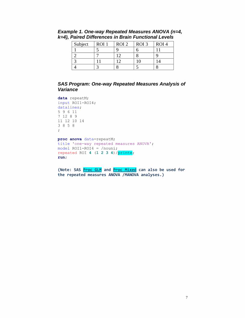
Example 1. One-way Repeated Measures ANOVA (n=4, k=4), Paired Differences in Brain Functional Levels

Subject ROI 1 ROI 2 ROI 3 ROI 4

1 5 9 6 11

2 7 12 8 9

3 11 12 10 14

4 3 8 5 8

SAS Program: One-way Repeated Measures Analysis of Variance

data repeatM;

input ROI1-ROI4;

datalines;

5 9 6 11

7 12 8 9

11 12 10 14

3 8 5 8

;

proc anova data=repeatM;

title 'one-way repeated measures ANOVA';

model ROI1-ROI4 = /nouni;

repeated ROI 4 (1 2 3 4)/printe;

run;

(Note: SAS Proc GLM and Proc Mixed can also be used for the repeated measures ANOVA /MANOVA analyses.)

8

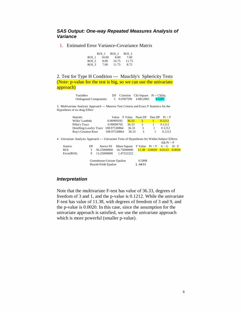
SAS Output: One-way Repeated Measures Analysis of Variance

1. Estimated Error Variance-Covariance Matrix

ROI_1 ROI_2 ROI_3

ROI_1 10.00 8.00 7.00

ROI_2 8.00 16.75 11.75

ROI_3 7.00 11.75 8.75

2. Test for Type H Condition --- Mauchly's Sphericity Tests

(Note: p-value for the test is big, so we can use the univariate

approach)

Variables DF Criterion Chi-Square Pr > ChiSq

Orthogonal Components 5 0.0587599 4.8812865 0.4305

3. Multivariate Analysis Approach --- Manova Test Criteria and Exact F Statistics for the

Hypothesis of no drug Effect

Statistic Value F Value Num DF Den DF Pr > F

Wilks' Lambda 0.00909295 36.33 3 1 0.1212

Pillai's Trace 0.99090705 36.33 3 1 0.1212

Hotelling-Lawley Trace 108.97530864 36.33 3 1 0.1212

Roy's Greatest Root 108.97530864 36.33 3 1 0.1212

4. Univariate Analysis Approach --- Univariate Tests of Hypotheses for Within Subject Effects

Adj Pr > F

Source DF Anova SS Mean Square F Value Pr > F G - G H - F

ROI 3 50.25000000 16.75000000 11.38 0.0020 0.0123 0.0020

Error(ROI) 9 13.25000000 1.47222222

Greenhouse-Geisser Epsilon 0.5998

Huynh-Feldt Epsilon 1.4433

Interpretation

Note that the multivariate F-test has value of 36.33, degrees of

freedom of 3 and 1, and the p-value is 0.1212. While the univariate

F-test has value of 11.38, with degrees of freedom of 3 and 9, and

the p-value is 0.0020. In this case, since the assumption for the

univariate approach is satisfied, we use the univariate approach

which is more powerful (smaller p-value).

9

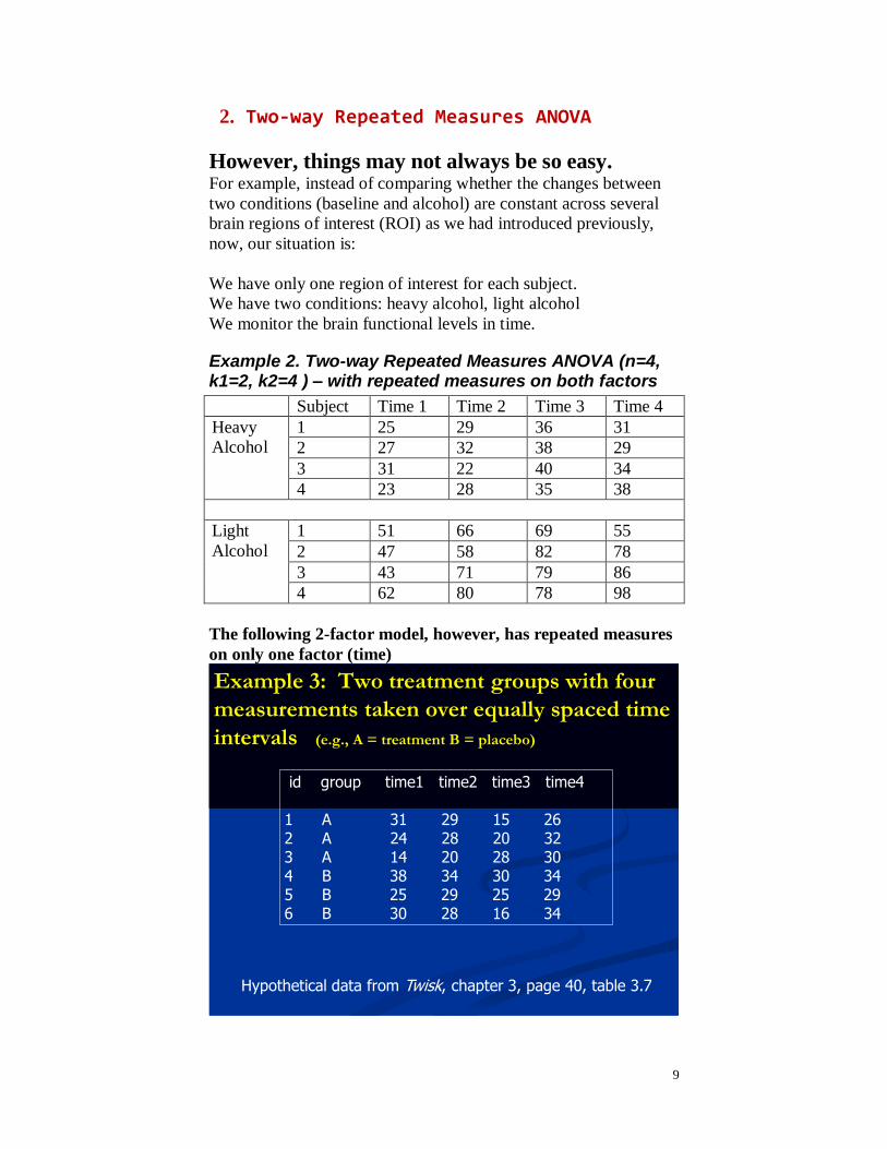
2. Two-way Repeated Measures ANOVA

However, things may not always be so easy. For example, instead of comparing whether the changes between

two conditions (baseline and alcohol) are constant across several

brain regions of interest (ROI) as we had introduced previously,

now, our situation is:

We have only one region of interest for each subject.

We have two conditions: heavy alcohol, light alcohol

We monitor the brain functional levels in time.

Example 2. Two-way Repeated Measures ANOVA (n=4, k1=2, k2=4 ) – with repeated measures on both factors

Subject Time 1 Time 2 Time 3 Time 4

Heavy

Alcohol

1 25 29 36 31

2 27 32 38 29

3 31 22 40 34

4 23 28 35 38

Light

Alcohol

1 51 66 69 55

2 47 58 82 78

3 43 71 79 86

4 62 80 78 98

The following 2-factor model, however, has repeated measures

on only one factor (time)

Example 3: Two treatment groups with four

measurements taken over equally spaced time

intervals (e.g., A = treatment B = placebo)

id group time1 time2 time3 time4

1 A 31 29 15 262 A 24 28 20 323 A 14 20 28 304 B 38 34 30 345 B 25 29 25 296 B 30 28 16 34

Hypothetical data from Twisk, chapter 3, page 40, table 3.7

10

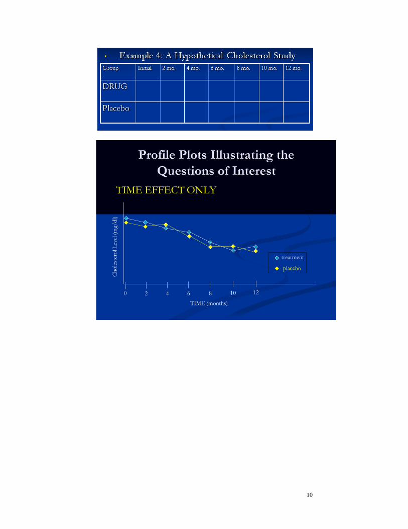
Profile Plots Illustrating the

Questions of Interest

TIME EFFECT ONLY

treatment

placebo

TIME (months)

2 4 6 8 10 12

Ch

ole

ster

ol L

evel

(m

g/d

l)

0

11

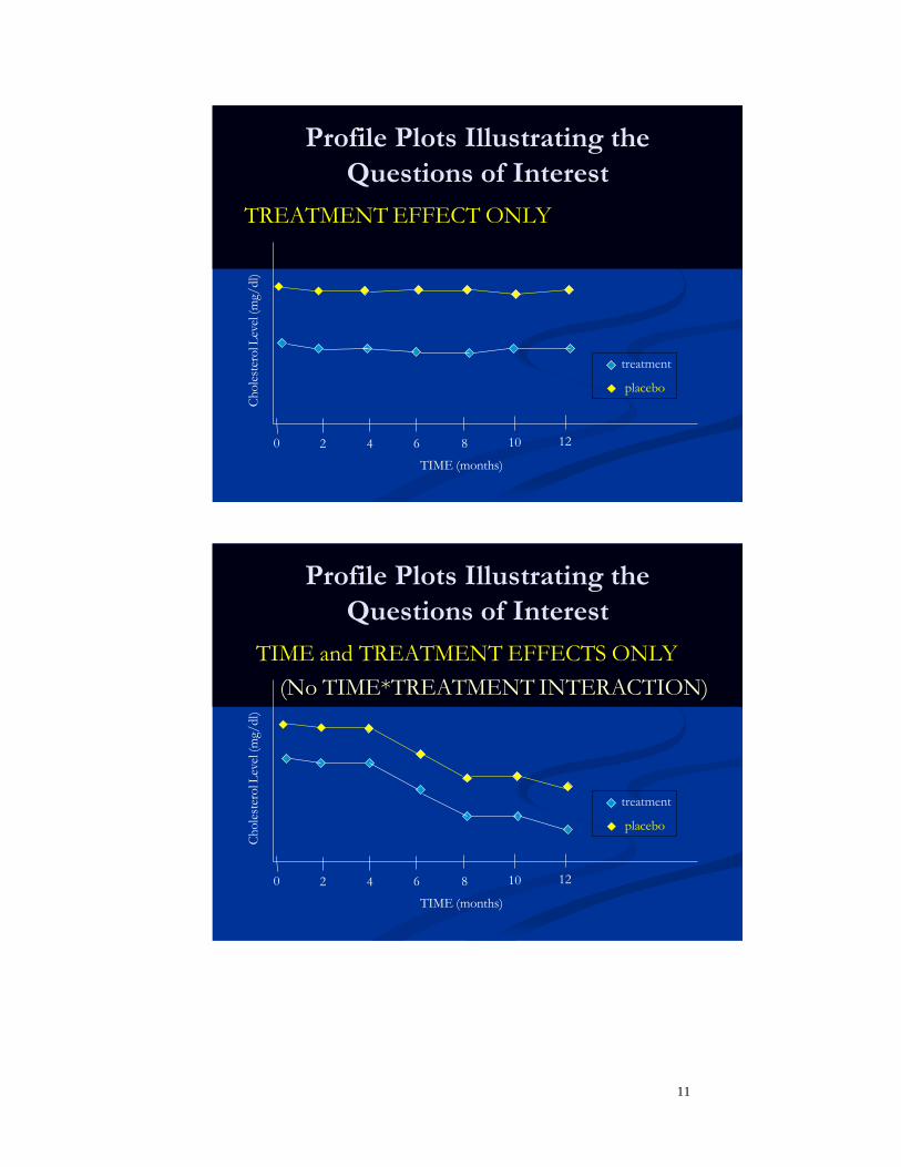
Profile Plots Illustrating the

Questions of Interest

TREATMENT EFFECT ONLY

treatment

placebo

TIME (months)

2 4 6 8 10 12

Ch

ole

ster

ol L

evel

(m

g/d

l)

0

Profile Plots Illustrating the

Questions of Interest

TIME and TREATMENT EFFECTS ONLY

(No TIME*TREATMENT INTERACTION)

treatment

placebo

TIME (months)

2 4 6 8 10 12

Ch

ole

ster

ol L

evel

(m

g/d

l)

0

12

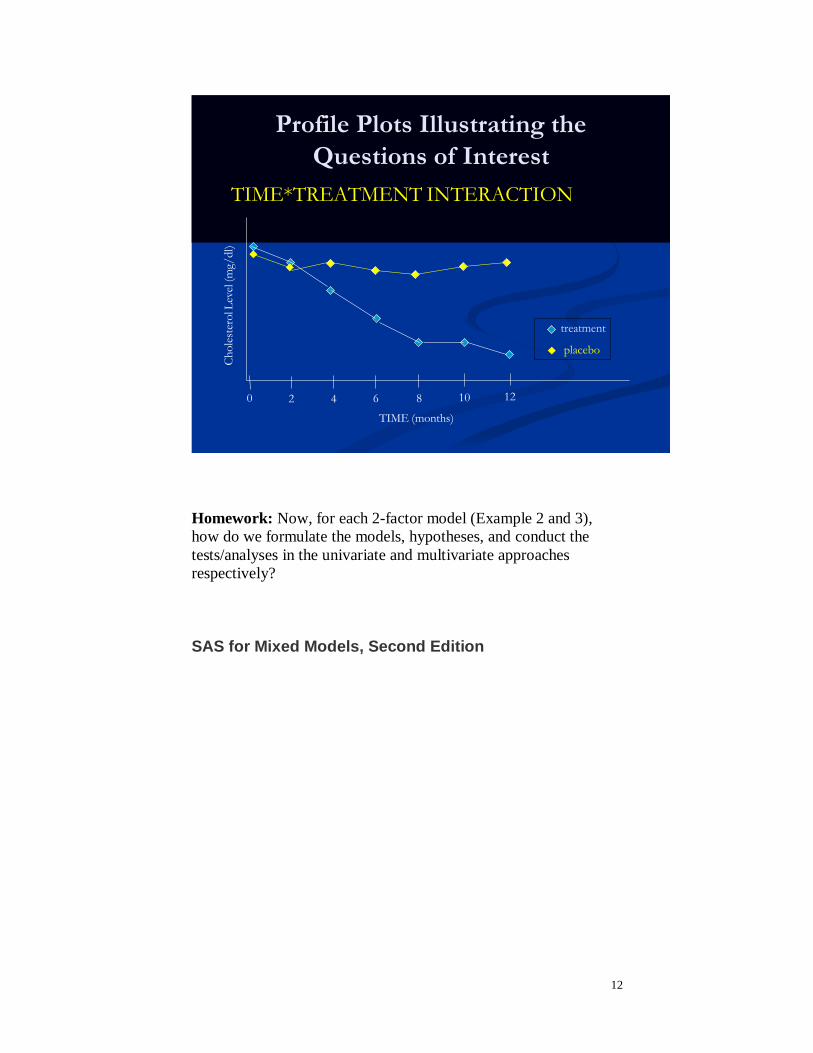
Profile Plots Illustrating the

Questions of Interest

TIME*TREATMENT INTERACTION

treatment

placebo

TIME (months)

2 4 6 8 10 12

Ch

ole

ster

ol L

evel

(m

g/d

l)

0

Homework: Now, for each 2-factor model (Example 2 and 3),

how do we formulate the models, hypotheses, and conduct the

tests/analyses in the univariate and multivariate approaches

respectively?

SAS for Mixed Models, Second Edition