![Model 707751 Waveform Editor - cdn.tmi.yokogawa.com · XXXXnnn.wvf. . . Specify any one set [Example of a file that is not supported] XXXX001.hdr XXXX001.wvf XXXX002.wvf Header file](https://static.fdocuments.us/doc/165x107/5af5ec267f8b9a4d4d8fb91d/model-707751-waveform-editor-cdntmi-specify-any-one-set-example-of-a.jpg)
&O WVF EF M PCUFOUJPO EV - Archive ouverte HAL
154
et discipline ou spécialité Jury : le Institut National des Sciences Appliquées de Toulouse (INSA de Toulouse) Clément Coïc jeudi 1 décembre 2016 Model-Aided Design of a High-Performance Fly-by-Wire Actuator, Based on a Global Modelling of the Actuation System using Bond-graphs ED MEGEP : Génie mécanique, mécanique des matériaux ICA, CNRS UMR 5312 Eric Bideaux, Professeur, INSA de Lyon, Rapporteur Esteban Codina, Professeur, Université Polytechnique de Catalogne, Rapporteur Jean-Charles Maré, Professeur, INSA de Toulouse, Directeur de Thèse Marc Budinger, Maître de Conférences (HDR), INSA de Toulouse, Examinateur Boris Grohmann, Docteur, Airbus Helicopters, Examinateur Jean-Romain Bihel, Ingénieur, Airbus Helicopters, Co-encadrant de Thèse Bruno Chaduc, Ingénieur, Airbus Helicopters, Invité Thibaut Marger, Docteur, Airbus Helicopters, Invité Jean-Charles Maré
Transcript of &O WVF EF M PCUFOUJPO EV - Archive ouverte HAL

et discipline ou spécialité
Jury :
le
Institut National des Sciences Appliquées de Toulouse (INSA de Toulouse)
Clément Coïc
jeudi 1 décembre 2016
Model-Aided Design of a High-Performance Fly-by-Wire Actuator,
Based on a Global Modelling of the Actuation System using Bond-graphs
ED MEGEP : Génie mécanique, mécanique des matériaux
ICA, CNRS UMR 5312
Eric Bideaux, Professeur, INSA de Lyon, Rapporteur
Esteban Codina, Professeur, Université Polytechnique de Catalogne, Rapporteur
Jean-Charles Maré, Professeur, INSA de Toulouse, Directeur de Thèse
Marc Budinger, Maître de Conférences (HDR), INSA de Toulouse, Examinateur
Boris Grohmann, Docteur, Airbus Helicopters, Examinateur
Jean-Romain Bihel, Ingénieur, Airbus Helicopters, Co-encadrant de Thèse
Bruno Chaduc, Ingénieur, Airbus Helicopters, Invité
Thibaut Marger, Docteur, Airbus Helicopters, Invité
Jean-Charles Maré

COÏC CLÉMENT – MODEL-AIDED DESIGN OF A HIGH-PERFORMANCE FLY-BY-WIRE ACTUATOR 2
ACKNOWLEDGEMENTS
The researches involved in this PhD dissertation are the fruit of collaboration between Institut
Clément Ader (Toulouse) on one side and Airbus Helicopters (Marignane) on the other side. It is thus
naturally that I would like to thank both entities for their agreement on supporting this work.
First, my gratitude is directed to my advisor Professor Jean-Charles Maré for his support all along
these three years. By sharing his knowledge, he gave me the ambition to look always further in a
direction. His availability was a key for my achievements: confirming, improving or correcting my ideas
soon enough to put as much energy as possible on each subject. His motivation and assets for spreading
the knowledge make me improve my rigor and communication skills. Also, the degree of freedom he
let me is appreciated for making my own opinion on certain topics.
Naturally, I would like to thanks Jean-Romain Bihel (technical referent) and Bruno Chaduc (Head
of the Hydraulics & Flight Controls department) both for their support on the “company-side” of this
PhD. They supported me in so many aspects: technically – by their experience in hydraulics and flight
controls, financially – defending the projects I worked on inside the company, humanly – by being
giving the responsibilities and keys for my own evolution… For all that I consider them as an infinite
support inside Airbus Helicopters and clearly as friends.
I would like to thank also the member of the committee that were a source of improvements for my
dissertation. The time my reviewers, Professor Eric Bideaux and Professor Esteban Codina, dedicated
for their deep study of my work and criticizing the dissertation is invaluable. Professor Marc Budinger
always provided me helpful remarks. Dr. Boris Grohmann and Dr. Thibaut Marger, during the four and
a half year at Airbus Helicopters shared their knowledge with me. The remarks provided by all the
members of this committee surely made possible improving my dissertation.
Airbus Helicopters is, in my opinion, a single team spread in several departments that are all
working for the best technical solution. Without this team the result of these researches would not have
been the same. So many people are part of this team but I would like to name the main contributors.
Pierre Heng taught me the Fly-by-Wire world; Jean-Marie Allietta shared with me his infinite
knowledge in modelling and simulation; Dr. Pascal Izzo supported me in many activities (such as
hardware-related during my test bench development); Roméo Byzery integrated my hydraulic actuation
system modelling in its flight control laws so we could run full flight control system simulations; Jean-
François Lafisse, Antoine Maussion, Emmanuel Beaud were always available for a talk and for jokes...
The help of all these co-workers was possible thanks to Max Massimi and Dr. Jacques Bellera who
opened me the doors of the Fly-by-Wire team and included me in their projects and developments.
Airb
us H
elic
opte
rs®
2016 –
All
rights
reserv
ed
ACKNOWLEDGEMENTS
COÏC CLÉMENT – MODEL-AIDED DESIGN OF A HIGH-PERFORMANCE FLY-BY-WIRE ACTUATOR 3
In this team, I am really grateful to all my colleagues from the Hydraulics & Flight Controls
department. I want to particularly name: Anthony Caila was a reference in all serial program and safety
related questions I could have; Thomas Buro and Joseph Barthélemy were always available for
discussion and constructive remarks on my work; the “Heavy-team” including Nicolas Avril, Jean-Yves
Agresta and Bernard Gemmati were the source of many smiles in these last years; Gérard Couderc and
Christophe Kilhoffer for the many lunched we spent together… And all the others!
This team included many invaluable supports in my journey: Pascal Leguay was THE hydraulic
expert and a referent to me; Michel Vialle was the origine of the project behind this PhD; Emmanuel
Mermoz enabled starting this project by a joint feasibility study; François-Xavier Filias was financially
controlling and approving all the expenses required for test benches, travels... Finally, Pierre Maret and
Fabienne Fraisse showed me an infinite support until my last day at Airbus Helicopters.
I could not forget to thank the French organisms who made this PhD possible. First, the French
national research and technology association (ANRT) for enabling doctoral thesis to happen with an
industrial partner. Then the French Directorate General of Armaments (DGA) for supporting research
and technology programs.
Last but far to be the least, I am deeply grateful to my family to whom this dissertation is dedicated.
My wife Tina and son Yann let me the time, during nights and weekends, to investigate more solutions,
to write communications and this dissertation. Without their comprehension and support, this PhD might
not have been possible.
Airb
us H
elic
opte
rs®
2016 –
All
rights
reserv
ed
CONTENTS
COÏC CLÉMENT – MODEL-AIDED DESIGN OF A HIGH-PERFORMANCE FLY-BY-WIRE ACTUATOR 4
DISSERTATION INTRODUCTION
A STEP TOWARDS HIGH-PERFORMANCE HELICOPTER FLIGHT CONTROLS ............................ 10
BIBLIOGRAPHY.................................................................................................................................................. 13
CHAPTER 1: FROM MECHANICALLY POWERED TO ELECTRICALLY SIGNALLED,
THE INCREMENTAL EVOLUTION OF HELICOPTER FLIGHT CONTROLS .................................... 17
1. PROVIDE LIFT AND PROPULSIVE FORCES ................................................................................................. 17 1.1. Generate Aerodynamic Forces ...................................................................................................... 17 1.2. Generate Lift ................................................................................................................................. 18 1.3. Control and Withstand Lift Forces ................................................................................................ 18 1.4. Control and Withstand Anti-Torque Forces .................................................................................. 20
2. PROVIDE H/C CONTROL AND STABILIZATION – CONVENTIONAL FLIGHT CONTROLS.............................. 21 2.1. Capture Pilots Intentions on Control Axes .................................................................................... 21 2.2. Transmit and Process Pilot Orders to Main and Tail Rotors........................................................ 21 2.3. Provide Stability & Control on Helicopter Axes ........................................................................... 23 2.4. Withstand Rotor Flight Loads – Hydro-Mechanical Actuators..................................................... 25
3. PROVIDE H/C CONTROL AND STABILIZATION – FBW FLIGHT CONTROLS ............................................... 29 3.1. Capture Pilot Intentions on Control Axes ..................................................................................... 30 3.2. Transmit Pilots Orders to Main and Tail Rotors .......................................................................... 30 3.3. Provide Stability & Control on Helicopter Axes ........................................................................... 30 3.4. Withstand Rotor Flight Loads – FbW Actuators ........................................................................... 31
4. FUTURE OF HELICOPTERS FLIGHT CONTROLS ......................................................................................... 39 4.1. FbW Retrofit – SIA ........................................................................................................................ 39 4.2. Fly-by-Light ................................................................................................................................... 39 4.3. Power-by-Wire .............................................................................................................................. 40 4.4. Individual Blade Control ............................................................................................................... 40 4.5. Dynamic Systems in Main Gear Box ............................................................................................. 41
5. CONCLUSION ........................................................................................................................................... 42 BIBLIOGRAPHY.................................................................................................................................................. 43
CHAPTER 2: ACTUATION SYSTEM MODELLING & SIMULATION ................................................... 49
1. INTRODUCTION ........................................................................................................................................ 49 1.1. Modelling and Simulation Terminology ........................................................................................ 49 1.2. Role of Modelling and Simulation in a New Development ............................................................ 52 1.3. Modelling & Simulation Errors .................................................................................................... 53
2. MODEL ARCHITECTING ........................................................................................................................... 54 2.1. Selected Modelling Needs ............................................................................................................. 55 2.2. Bond-graph Formalism ................................................................................................................. 57 2.3. Proposed Concepts Defined by Modelling Needs ......................................................................... 59 2.4. Proposed Standardization of the Mechanical Domain .................................................................. 61 2.5. Modelling Fluid Power Systems with Bond-graphs ...................................................................... 65 2.6. Electrical Systems with Bond-graphs ............................................................................................ 68
3. ACTUATION SYSTEM VIRTUAL MODEL ................................................................................................... 68 3.1. Purpose of Actuation System modelling ........................................................................................ 68 3.2. Fluid Modelling ............................................................................................................................. 70 3.3. Hydraulic System Virtual Model ................................................................................................... 73 3.4. FbW Actuator Virtual Model ......................................................................................................... 85
4. ACTUATION SYSTEM SIMULATION .......................................................................................................... 96 4.1. Load Contribution To Performance .............................................................................................. 96 4.2. Temperature Contribution To Performance .................................................................................. 98 4.3. Actuator Couplings ....................................................................................................................... 99 4.4. Actuation System Simulation ....................................................................................................... 101
5. CONCLUSION ......................................................................................................................................... 102 BIBLIOGRAPHY................................................................................................................................................ 103
Airb
us H
elic
opte
rs®
2016 –
All
rights
reserv
ed

CONTENTS
COÏC CLÉMENT – MODEL-AIDED DESIGN OF A HIGH-PERFORMANCE FLY-BY-WIRE ACTUATOR 5
CHAPTER 3: METHODS OF LINEAR FLUID BEARING DESIGN UNDER AEROSPACE
CONSTRAINTS ................................................................................................................................................ 109
1. STUDY OF A FLUID FILM – REYNOLDS EQUATION ................................................................................. 110 1.1. Fluid Film under Study ............................................................................................................... 110 1.2. Continuity Equation .................................................................................................................... 111 1.3. Surface Flow Rate Calculation ................................................................................................... 112 1.4. Reynolds Equation....................................................................................................................... 112
2. CREATING A NORMAL FORCE IN FLUID BEARINGS ................................................................................ 114 2.1. Constant Height Fluid Film ........................................................................................................ 114 2.2. Constant Height Gradient Fluid Film ......................................................................................... 116 2.3. Discontinuous Height Fluid Film ................................................................................................ 118 2.4. Solution Selection ........................................................................................................................ 120
3. DESIGN OF HYDROSTATIC THRUST BEARINGS UNDER AEROSPACE CONSTRAINTS ................................ 122 3.1. Background ................................................................................................................................. 122 3.2. Temperature Sensitivity ............................................................................................................... 122 3.3. A New Type of Fixed Restriction – The Short Tube Orifice ........................................................ 124 3.4. Pre-Sizing Optimization .............................................................................................................. 129 3.5. Conclusion................................................................................................................................... 132
4. DESIGN OF CONICAL HYBRID BEARINGS UNDER AEROSPACE CONSTRAINTS ........................................ 133 4.1. Background ................................................................................................................................. 133 4.2. Temperature and Eccentricity Sensitivity .................................................................................... 134 4.3. Design Parameter Sensitivities ................................................................................................... 137 4.4. Conclusion................................................................................................................................... 139
5. CONCLUSION ......................................................................................................................................... 140 BIBLIOGRAPHY................................................................................................................................................ 141
DISSERTATION CONCLUSION................................................................................................................... 147
Airb
us H
elic
opte
rs®
2016 –
All
rights
reserv
ed

COÏC CLÉMENT – MODEL-AIDED DESIGN OF A HIGH-PERFORMANCE FLY-BY-WIRE ACTUATOR 6
INTRODUCTION GENERALE
VERS DES COMMANDES DE VOL D’HELICOPTERE PLUS PERFORMANTES
Les commandes de vol d’hélicoptères intègrent généralement des actionneurs hydrauliques. Ils
assistent le pilote et l’autopilote en effort en positionnant le plateau cyclique selon les ordres d’entrée
(typiquement avec une bande passante de quelques Hertz) tout en rejetant les perturbations liées aux
charges en provenance du rotor (typiquement quelques dizaines de Hertz). En réponse à une demande
du marché, l’augmentation du confort des passagers, Airbus Helicopters souhaite implémenter de
nouvelles fonctions au sein du système de commandes de vol, tel le contrôle actif du rotor. Ces dernières
nécessitent le contrôle en position des actionneurs à des fréquences multiples de celle du rotor (par
exemple, 19 Hertz pour le rotor 3-pales du SA 349 [POL86]).
Pour ce faire, deux axes principaux ont été identifiés et investigués dans ce manuscrit :
1. Développer de nouvelles technologies permettant l’implémentation de ces nouvelles fonctions.
2. Evaluer les nouveaux designs grâce à l’utilisation de modèles virtuels et leurs simulations.
En ce qui concerne le premier axe, le choix technologique des systèmes de guidage et d’étanchéité
des vérins d’actionneurs actuels est incompatible avec des sollicitations hautes fréquences. Les moyens
de guidage recentrent l’ensemble piston-tige dans le corps du vérin. Les moyens d’étanchéités
empêchent le passage du fluide au niveau des surfaces étanchéifiées. Sur les actionneurs hydrauliques
d’hélicoptère, la fonction de guidage est généralement réalisée par des paliers en aluminium ou en
bronze alors que la fonction d’étanchéité est souvent assurée par une combinaison de joints élastomères
et plastomères. Un déplacement de l’actionneur à haute fréquence endommagerait dramatiquement les
joints et conduirait à une fuite hydraulique inacceptable au niveau des paliers de guidage. Cette fuite
pourrait alors avoir lieu au niveau du piston (entre les chambres d’extension et rétraction) ou au niveau
des paliers externes (entre les chambres et l’environnement). Un vérin d’actionneur hydraulique est
présenté en Figure 1 détaillant les sous-ensembles dont la terminologie a été utilisée précédemment.
De nouvelles technologies avec un design adapté doivent donc être développées afin de permettre
l’implémentation de ces fonctions nécessitant de hautes fréquences. Les vérins hautes performances
disponibles dans l’industrie, notamment pour les bancs d’essais de fatigue ou d’endurance, utilisent des
paliers linéaires fluides. Un palier fluide consiste à laisser passer un fin film de fluide pressurisé, lequel
génère une force normale au palier. La contrepartie de cette technologie est une fuite fonctionnelle de
fluide drainée vers la ligne retour. Leur développement et utilisation dans l’industrie est facilité par un
apport en fluide à pression et température quasi-constante.
Airb
us H
elic
opte
rs®
2016 –
All
rights
reserv
ed

INTRODUCTION GENERALE
COÏC CLÉMENT – MODEL-AIDED DESIGN OF A HIGH-PERFORMANCE FLY-BY-WIRE ACTUATOR 7
Le palier fluide est une solution technologique intéressante pour atteindre les hautes performances
des actionneurs tout en maintenant une durée de vie acceptable. Cependant, dans le cas précis d’un
système de puissance embarqué, tel que le système hydraulique d’un hélicoptère, le design des paliers
fluides linéaires n’est pas trivial : la température du fluide varie énormément, typiquement cette
variation peut représenter plus de 150°C, et avec elle, les propriétés intrinsèques du fluide. Une étude
détaillée des performances du palier fluide sur l’ensemble du spectre de température est donc nécessaire.
D’autres avantages s’ajoutent à l’utilisation de paliers fluides, en plus de la potentielle
augmentation des performances de l’actionneur :
- La défaillance du joint de piston est une panne dormante, ce qu’elle ne peut être détectée sans un
test dédié. Cela contraint le planning de maintenance de l’actionneur et induit un coût non-
négligeable pour le client. De ce fait, la suppression des joints de piston est une avancée
considérable.
- Le fluide utilisé par l’actionneur peut être partagé avec d’autres composants. Par exemple, des
ensembles mécaniques, telle la boîte de transmission principale, pourrait être lubrifiés par le fluide
en provenance du drain de l’actionneur.
- Le partage du fluide permet d’envisager l’usage d’un unique échangeur thermique pour plusieurs
sous-systèmes, conduisant ainsi à un gain de masse au niveau hélicoptère.
- Aussi, l’utilisation d’un unique échangeur thermique améliorerait son efficacité pour le système
hydraulique et permettrait donc de réduire la plage de température dans lequel le fluide évolue.
Le système d’actionnement de l’hélicoptère, composé de la génération de puissance hydraulique,
sa distribution ainsi que sa consommation, pourra donc être optimisé dans le but de minimiser sa
masse.
Au regard de tous ces avantages, l’utilisation de paliers fluides pour actionneurs intégrés dans une
enveloppe a été breveté, avec notre contribution, par Airbus Helicopters [COI15a]. Une vue du brevet
est présentée en Figure 2 (a). En continuité du brevet, l’auteur a aussi contribué à l’étude de possible
implémentation dont une solution est montrée en Figure 2 (b). Cette invention possède l’avantage
supplémentaire de protéger les actionneurs d’agressions extérieures (e.g. impact à l’oiseau).
Bien que ce ne soit pas une obligation pour l’application de ce brevet, l’utilisation d’un système de
commandes de vol électrique contribue à augmenter la bande passante de l’actionnement, à faciliter
l’introduction de nouvelles fonctions et à en améliorer la fiabilité.
Le temps nécessaire au développement de nouvelles technologies peut être réduit grâce à la
modélisation et simulation virtuelle du système concerné. Les modèles virtuels doivent être conçus dans
le but de reproduire le comportement du système et de ses sous-systèmes de manière à pouvoir réaliser
les tests unitaires et d’intégration d’intérêt. Dans notre cas, le système d’actionnement doit être modélisé
Airb
us H
elic
opte
rs®
2016 –
All
rights
reserv
ed
INTRODUCTION GENERALE
COÏC CLÉMENT – MODEL-AIDED DESIGN OF A HIGH-PERFORMANCE FLY-BY-WIRE ACTUATOR 8
afin de reproduire virtuellement les réponses d’une implémentation existante. Il doit aussi faciliter
l’évaluation de nouveaux designs partiels ou complets du système. Sur la base de ces observations, un
intérêt particulier a été porté sur l’architecture des modèles afin de permettre leur réutilisation et leur
évolution incrémentale. L’impact de la technologie choisie sur la modélisation du système doit être
minimiser afin d’évaluer de manière efficace plusieurs architecture. Cela a été possible grâce à un travail
de standardisation des interfaces des modèles.
Ces travaux de recherche ont pour but l’investigation de l’augmentation de performance des
actionneurs à commandes de vol électriques et l’impact induit sur le système de génération et
distribution hydraulique. Ces recherches représentent donc un pas en avant dans l’application du brevet
présenté ci-dessus. Dans le but de synthétiser ces travaux, ce mémoire est organisé en quatre chapitres :
Le Chapitre 1 présente les concepts généraux d’un système de commandes de vol d’hélicoptère.
Il met en évidence ses évolutions incrémentales dirigées par les besoins naissants, depuis les commandes
de vol mécaniques jusqu’aux électriques. Une attention particulière est portée aux différentes
architectures et technologies d’actionneurs conduisant à des recommandations sur le choix
technologique en lien avec la criticité de la fonction à réaliser.
Le Chapitre 2 propose une modélisation virtuelle du système d’actionnement avec l’aide du
formalisme Bond-graph. Le modèle est adressé avec une vision orientée objet et de manière à ce que les
paramètres à renseigner soient ceux dont les ingénieurs disposent. Cette modélisation a pour but de
réduire le temps de développement d’un nouveau système d’actionnement de commandes de vol
d’hélicoptère tout en assurant une meilleure satisfaction des exigences spécifiées. Elle permet aussi,
dans le cadre de l’augmentation des performances du système d’actionnement, de prédire les limitations
au niveau de l’actionneur induites par l’ensemble du système, par exemple dû à la température du fluide
ou encore par la génération et distribution hydraulique.
Le Chapitre 3 se focalise sur les technologies de paliers fluides linéaires. Dans un premier temps,
l’équation de Reynolds est détaillée. Elle fournit une modélisation algrébrico-différentielle de la
distribution de pression au sein du film de fluide. Sur la base de cette équation, différentes formes de
paliers sont étudiées dans le but d’observer leur impact sur trois critères principaux de dimensionnement
du palier : sa force normale, sa fuite et sa raideur. Ensuite, un processus de pré-dimensionnement d’une
butée hydrostatique est proposé, en insérant un « orifice tube-court » en tant que restriction amont
nécessaire à la raideur du palier. Ce type d’orifice introduit un paramètre de dimensionnement d’intérêt,
lequel peut aisément être adapté de manière à répondre au dilemme force/raideur versus débit de fuite
sur la plage de variation de température du fluide. Finalement, une étude de sensibilité est menée sur les
paliers hybrides coniques. Elle adresse la variation des trois principaux critères de dimensionnement
Airb
us H
elic
opte
rs®
2016 –
All
rights
reserv
ed

INTRODUCTION GENERALE
COÏC CLÉMENT – MODEL-AIDED DESIGN OF A HIGH-PERFORMANCE FLY-BY-WIRE ACTUATOR 9
face aux variables temporelles (i.e. température et excentration), ainsi que face aux paramètres de
dimensionnement (i.e. la forme du palier).
Le Chapitre 4 présente un développement, assisté par les modèles virtuels, d’actionneur hautes
performances, utilisant une technologie de paliers fluides linéaires. Ce chapitre est une contribution à
un projet de recherche Airbus Helicopters. Dû aux sauts technologiques portés par l’ensemble du projet,
ce chapitre a été jugé confidentielle pour une durée de dix ans.
Finalement, la Conclusion Générale résume les principales avancées de ces travaux et liste les
perspectives associées à chaque sujet traité dans ce mémoire.
Airb
us H
elic
opte
rs®
2016 –
All
rights
reserv
ed

COÏC CLÉMENT – MODEL-AIDED DESIGN OF A HIGH-PERFORMANCE FLY-BY-WIRE ACTUATOR 10
DISSERTATION INTRODUCTION
A STEP TOWARDS HIGH-PERFORMANCE HELICOPTER FLIGHT CONTROLS
Helicopter flight control systems usually integrate hydraulic actuators. They assist the pilot and
autopilot in effort by positioning the swashplate according to the input commands (typically with a
bandwidth of a few Hertz) while rejecting the effect of load disturbances coming from the rotor
(typically with a bandwidth of a few tens of Hertz). As a response to a market demand, which is to
increase passenger comfort, Airbus Helicopters would like to implement new functions on the flight
control system, such as active rotor control. This requires controlling the actuator position at the rotor
frequencies (e.g. 19 Hertz for a 3-blade rotor [POL86]).
For this, two main axes have been identified and are investigated in this dissertation:
1. To develop new technologies enabling the implementation of these new functions.
2. To evaluate the new design by resorting to modelling and simulation.
With regard to technology improvement, current bearing and sealing devices on actuator cylinders
are not designed to face such high frequencies. Indeed, bearing devices guide the actuator piston-rod
assembly in the housing cylinder (or vice versa) while sealing devices prevent leakage through the sealed
surfaces. On helicopter actuators, the guiding function is typically fulfilled by aluminium or bronze
rings, whereas the sealing function is usually performed by a combination of elastomeric and
plastomeric seals. High-frequency motion wears the dynamic seals dramatically, leading to unacceptable
leakage at the guiding rings. Leakage can occur at piston level (between the extension and retraction
chambers) and at bushing level (between one chamber and the environment). A hydraulic cylinder of an
actuator is presented in Figure 1 and the elements corresponding to the terminology used are shown.
PISTON
BEARING & SEALING DEVICES
BUSHING
BEARING & SEALING DEVICESROD
HOUSINGEXTENSION
CHAMBER
RETRACTION
CHAMBER
Figure 1 – Dynamic bearing and sealing devices in a hydraulic cylinder, modified from [FAI06].
A re-engineering of both the actuator bearing and the sealing functions is thus required in order to
enable the implementation of high-frequency functions. Industrial high-performance actuators, typically
Airb
us H
elic
opte
rs®
2016 –
All
rights
reserv
ed

DISSERTATION INTRODUCTION
COÏC CLÉMENT – MODEL-AIDED DESIGN OF A HIGH-PERFORMANCE FLY-BY-WIRE ACTUATOR 11
used for fatigue or endurance test benches, include piston and bushing linear fluid bearings at the cost
of a functional leakage drained to the return line. A fluid bearing consists in a fluid film, the pressure of
which generates a bearing force. Their development and operation is facilitated if the bearing is supplied
at constant pressure and temperature.
The linear fluid bearing is an interesting technology to achieve high-performance actuators without
excessive lifespan reduction. However, in case of embedded power systems such as the hydraulic
network on helicopters, the design of linear fluid bearings is not simple: the temperature varies widely,
typically within a range of more than 150°C, and with it the fluid properties. An investigation of the
linear fluid bearing performances over such an extended range of temperature is thus required.
In addition to enabling enhanced performance, the removal of conventional sealing devices has
other advantages:
- The piston seal failures are dormant, which means that they cannot be detected without a
dedicated test. This constrains the maintenance planning of the actuator and has hence a non-
negligible cost for the customers. From this point of view, removing seals obviously marks a step
forward.
- The actuator fluid could be shared with other applications. For example, mechanical parts, such
as the main gear box, could be lubricated with the fluid coming out of the actuator drain.
- The fluid sharing allows designing a single heat exchanger for the various applications. This leads
to a mass reduction at helicopter level.
- Indeed, having a single heat exchanger ensures a more efficient fluid heating or cooling. Thus,
the operating temperature range can be reduced. The Actuation System, composed of the
hydraulic power generation and distribution and its consumers (such as the actuators) can thus be
better optimized and its mass can be minimized.
With regard to these advantages, the use of fluid bearings for actuators integrated in an enclosure
has been patented, with our contribution, by Airbus Helicopters [COI15a]. On the left side of Figure 2,
a view of the patent drawing is shown. Following this patent, the author has also contributed to the study
of a possible implementation, which is presented on the right side of Figure 2. Another advantage of this
invention is actuator protection from external aggression (e.g. bird strike).
Although it is not mandatory for applying this patent, resort to a Fly-by-Wire flight control system
contributes to an increased actuation bandwidth, the provision of new functions and improved reliability.
Airb
us H
elic
opte
rs®
2016 –
All
rights
reserv
ed

DISSERTATION INTRODUCTION
COÏC CLÉMENT – MODEL-AIDED DESIGN OF A HIGH-PERFORMANCE FLY-BY-WIRE ACTUATOR 12
(a) –Variant as patented in [COI15a] (b) – Possible implementation [ETM14]
Figure 2 – High-performance actuator in Main Gear Box.
The development time of new technologies can be reduced with the help of virtual model
simulation. Virtual models should be designed to reproduce system and subsystem behaviour in order
to perform unitary and integration virtual tests. In our application, the Actuation System must be
modelled to reproduce the responses of existing designs and to facilitate and evaluate new designs of
the entire system or some of its component. Based on these observations, a particular focus has to be
put on architecting the model to allow its reusability and incremental evolution. The impact of the
technology selection on the system modelling shall be minimized in order to be able to efficiently
evaluate several architectures.
This research aims at investigating the Fly-by-Wire actuator performance improvements and its
impact on the hydraulic power generation and distribution system, as a step towards the presented patent
implementation. For this purpose, the dissertation is organized in four chapters.
Chapter 1 presents the general concepts of the helicopter flight control system. It highlights the
incremental need-driven evolution from the mechanical to the Fly-by-wire technology flight control
system. In this chapter, a particular focus is put on the actuator architectures and technologies.
Recommendations on the actuator technology are given.
Chapter 2 proposes a virtual modelling of the Actuation System with the support of the Bond-
graph formalism. The model is addressed in an object-oriented manner, paying attention to involve
parameters that engineers are able to provide. It is aimed at reducing the development time of a new
helicopter Actuation System and at ensuring a better fulfilment of its specification. Within the scope of
increasing Actuation System performance, it permits predicting the limitations at actuator level, which
are for example induced by the temperature or by the hydraulic power generation and distribution.
Airb
us H
elic
opte
rs®
2016 –
All
rights
reserv
ed
DISSERTATION INTRODUCTION
COÏC CLÉMENT – MODEL-AIDED DESIGN OF A HIGH-PERFORMANCE FLY-BY-WIRE ACTUATOR 13
Chapter 3 focuses on the linear fluid bearing technologies. It starts by detailing the Reynolds
equation, which provides the differential equation modelling the pressure distribution in the fluid film.
Based on this, different physical shapes of the bearings are studied to observe their impact on the three
main design criteria of fluid bearings: bearing force, leakage and stiffness. Then, a pre-sizing process of
hydrostatic thrust bearings is proposed, introducing a short tube orifice as the fixed restriction required
for stiffness. The short tube orifice introduces an interesting design parameter that can easily be managed
to solve the sizing dilemma for meeting the bearing performance requirements. Finally, a sensitivity
study is conducted on conical hybrid bearings. It addresses the variation of the three main design criteria
with time variables (i.e. temperature and eccentricity) and then with design parameters (i.e. the physical
shape of the bearing).
Chapter 4 is restricted and removed from this dissertation.
Finally, the Dissertation Conclusion summarizes the main achievements of this research and
provides the perspectives for each subject dealt with in this dissertation.
BIBLIOGRAPHY
[COI15a] COÏC, C., BIHEL, J.-R., MARGER, T. & COUDERC, C., Patent US2015298796 (A1) -
Aircraft Hydraulic System Comprising at least one Servo-Control, and an Associated
Rotor and Aircraft. Airbus Helicopters, France, 2015.
[ETM14] ETM, Flight Controls Inside the Rotor Mast. Airbus Helicopters, France, 2015.
(internal publication)
[FAI06] FAISANDIER, J., Mécanismes Hydrauliques et Pneumatiques. 9th edition, Dunod, Paris,
2006. (in French)
[POL86] POLYCHRONIADIS, M. & ACHACHE, M., Higher Harmonic Control: Flight Tests of an
Experimental System on SA 349 Research Gazelle. 42nd Annual Forum of the American
Helicopter Society, Washington, 1986.
Airb
us H
elic
opte
rs®
2016 –
All
rights
reserv
ed

COÏC CLÉMENT – MODEL-AIDED DESIGN OF A HIGH-PERFORMANCE FLY-BY-WIRE ACTUATOR 14
CHAPITRE 1
ÉVOLUTION INCREMENTALE DES COMMANDES DE VOL D’HELICOPTERE
1.1 PRINCIPAUX ASPECTS DE LA MECANIQUE DU VOL HELICOPTERE
Les forces propulsive et sustentatrice de l’hélicoptère proviennent de rotors. La rotation des pales
génère une force résultante, perpendiculaire au plan du rotor. L’orientation du rotor et la modulation de
l’effort résultant permettent de contrôler la trajectoire de l’hélicoptère.
L’équilibre des forces appliquées sur un hélicoptère en vol d’avancement est présenté en Figure 1.2.
La composante verticale de la résultante rotor est la portance (« lift » en anglais) – qui compense le poids
de l’hélicoptère – tandis que la composante horizontale est la poussée (« thrust » en anglais) – qui fournit
une accélération à la machine si elle est supérieure à la traînée aérodynamique engendrée par la vitesse.
L’intensité de la force résultante rotor peut être modulée en changeant l’incidence (ou pas) des
pales– et donc l’angle d’attaque du flux d’air. Comme cette action est commune, en amplitude, à toutes
les pales simultanément, elle est appelée variation du pas collectif (« collective pitch » en anglais).
L’orientation de cette force est possible grâce au pas cyclique qui change le pas des pales
individuellement. Le terme cyclique provient du fait que, pour une commande de pas cyclique donnée,
le pas des pales est le même à un azimut donné.
L’inclinaison de la résultante rotor induit des moments selon un des axes souhaités – présentés en
Figure 1.3 – (ou la combinaison d’axes souhaitée) et provoque les rotations de l’appareil. La variation
de la composante de cette résultante produira un déplacement dans la direction de l’axe associé.
Finalement l’hélicoptère peut évoluer selon les six degrés de liberté, car il est aussi capable tourner
autour de son mât rotor (c’est l’axe de lacet). Le couple transmis par le(s) moteur(s) au rotor principal
induit un couple de réaction dans la direction opposée sur l’hélicoptère qui doit être compensé. Une
surcompensation ou sous-compensation de ce couple permet une accélération angulaire autour de l’axe
de lacet – et donc de contrôler une position angulaire. Dans ce but, l’architecture la plus répandue
d’hélicoptères inclue un rotor anti-couple – ou rotor de queue. La rotation de l’hélicoptère autour de
l’axe de lacet est réalisée par action sur le pas collectif du rotor de queue.
1.2 ACTIONNEMENT A COMMANDES DE VOL MECANIQUES
Un hélicoptère présente ainsi classiquement quatre commandes de pilotage : le collectif, le tangage,
le roulis et le lacet. Sur la plupart des hélicoptères, les pilotes agissent sur deux manches et une paire de
pédales pour piloter l’attitude et la trajectoire de l’appareil :
Airb
us H
elic
opte
rs®
2016 –
All
rights
reserv
ed
CHAPITRE 1 – EVOLUTION INCREMENTALE DES COMMANDES DE VOL D’HELICOPTERE
COÏC CLÉMENT – MODEL-AIDED DESIGN OF A HIGH-PERFORMANCE FLY-BY-WIRE ACTUATOR 15
- Le manche collectif qui contrôle le pas collectif des pales
- Le manche cyclique lequel oriente le rotor en tangage et roulis
- Les pédales pour le contrôle de l’axe de lacet
Les premiers hélicoptères furent élaborés de manière à ce que le pilote soit capable de piloter sa
trajectoire, dans l’ensemble du domaine de vol, sans assistance hydraulique. Les commandes de vol se
résumaient alors à une combinaison de bielles, renvoies, leviers mécaniques et/ou câbles pour assurer la
transmission de la commande d’entrée pilote aux rotors principal et arrière. Pour exemple, l’Alouette II
– dont le système de commande de vol est présenté en Figure 1.5 – est un hélicoptère de 5 places qui a
réalisé son premier vol en 1955.
Le pas collectif des pales peut être contrôlé indépendamment des variations de pas cyclique, même
si les deux actions agissent au final sur les mêmes ensembles mécaniques – le plateau cyclique. La
commande de pas collectif est ajoutée à la commande de pas cyclique grâce au mélangeur (Figure 1.6).
L’augmentation des charges de vol conduit à l’ajout d’actionneur à commande mécanique et
puissance hydraulique dans le but de réduire les efforts de pilotage. Seulement quatre ans après le
premier vol de l’Alouette II, son successeur – l’Alouette III – apparut. Elle intégrait les premières
servocommandes hydrauliques (Figure 1.8).
L’intégration des servocommandes à l’intérieur de l’armoire commande de vol n’est pas usuelle
car elle nécessite de dimensionner les bielles qui vont jusqu’au rotor à l’effort de vol. La plupart du
temps, les servocommandes sont positionnées au-dessus du plancher mécanique.
Ceci conduit à trouver une solution avec trois actionneurs de rotor principal en repère fixe,
contrôlant l’orientation du plateau cyclique. Le rotor arrière est contrôlé par un seul actionneur.
Afin de garantir que la perte de la fonction commande de vol de l’hélicoptère est extrêmement
improbable, les servocommandes des appareils Airbus Helicopters possèdent, à quelques exceptions
près, deux corps hydrauliques positionnés en tandem (ou série) et alimentés par deux circuits
hydrauliques ségrégués.
1.3 ACTIONNEMENT A COMMANDES DE VOL ÉLECTRIQUES HELICOPTERE
Les commandes de vol électriques consistent à transmettre les commandes des pilotes grâce à des
signaux électriques jusqu’aux actionneurs via des calculateurs de contrôle de vol.
Pour cela, il est important de conserver les interfaces pilotes (manches et pédaliers) et les interfaces
d’actionnement mais de réaliser un « re-engineering » de la fonction complète. En effet, l’ensemble des
couplages de commandes de vol et limites des lois de pilotage sont intégrés dans le calculateur et peuvent
Airb
us H
elic
opte
rs®
2016 –
All
rights
reserv
ed

CHAPITRE 1 – EVOLUTION INCREMENTALE DES COMMANDES DE VOL D’HELICOPTERE
COÏC CLÉMENT – MODEL-AIDED DESIGN OF A HIGH-PERFORMANCE FLY-BY-WIRE ACTUATOR 16
donc être plus facilement modifiés. Ceci conduit donc à une fonction réalisée de manière plus adaptée à
l’appareil induisant de meilleures qualités de vol en termes de stabilité et facilité de pilotage.
Paradoxalement, malgré les problèmes de stabilité de mécanique du vol hélicoptère, en
comparaison des caractéristiques aérodynamiques avions – plus stables – l’installation de commandes
électriques sur avion est une solution banalisée, des avions militaires aux avions civils, alors que cette
technologie reste marginale dans le monde hélicoptère.
La difficulté de transposition de la technologie d’actionneurs du monde avion au monde hélicoptère
provient essentiellement du fait qu’il n’y a pas de redondance d’actionnement possible sur hélicoptère,
et qu’en surcroit les actionneurs hélicoptère sont dans un environnement très sévère.
Ceci revient à considérer les technologies actuellement mise en œuvre dans un contexte avion à la
lumière des contraintes particulières du contexte hélicoptère.
1.4 CONCEPTS D’ACTIONNEURS POSSIBLES A L’HORIZON 2020
A l’horizon 2020, différents concepts d’actionnements sont possibles pour application sur un futur
hélicoptère à commandes de vol électriques, sur la base des technologies actuellement mises en œuvre
dans le mode aéronautique. Dans ce chapitre, nous avons étudié les quatre technologies suivantes :
- L’actionneur électrohydraulique à actionnement direct du distributeur, référencé par DDV pour
« Direct Drive Valve » en anglais.
- L’actionneur électrohydraulique à actionnement du distributeur par amplification hydraulique de
la commande, appelé EHSV par la suite pour « Electro-Hydraulic ServoValve » en anglais.
- L’actionneur électromécanique en lieu et place de l’actionneur hydromécanique conventionnel,
appelé EMA pour « Electro-Mechanical Actuator » en anglais.
- L’actionneur électromécanique, et son calculateur d’asservissement, pilotant le levier d’entrée
d’une servocommande conventionnelle, dénommé SIA pour « Smart Interface Actuator » en
anglais.
Une attention particulière est portée au deux premières technologies dans la suite du chapitre en
anglais. Les deux autres sont pour leur part présentées en tant qu’opportunité pour le futur mais
manquent de maturité à ce jour.
Airb
us H
elic
opte
rs®
2016 –
All
rights
reserv
ed

COÏC CLÉMENT – MODEL-AIDED DESIGN OF A HIGH-PERFORMANCE FLY-BY-WIRE ACTUATOR 17
CHAPTER 1:
FROM MECHANICALLY POWERED TO ELECTRICALLY SIGNALLED,
THE INCREMENTAL EVOLUTION OF HELICOPTER FLIGHT CONTROLS
As a basis for a new development, it has been decided to first introduce the needs behind former
evolutions of the helicopter flight control system and their current and future trends. Airbus Helicopters,
drawing on its experience acquired over more than 60 years of helicopter production, established a
functional breakdown of rotorcraft. The titles of the first section of this chapter refer thus to the
functional breakdown of helicopters. Some functions have been slightly adapted to the particularities of
flight control systems, which are the scope of this chapter.
In order to understand the role of flight controls on helicopters, section 1 synthetically introduces
the principles of flying and details some existing architectures at rotorcraft level. Section 2 focuses on
mechanically signalled flight controls. The need-driven incremental evolution of flight control systems
is presented. Section 3 addresses the technological step from conventional to Fly-by-Wire (FbW) flight
controls. Two main technologies are used for electro-hydraulic actuators of FbW helicopters. A
particular focus is laid on these solutions in this section. The most promising evolution perspectives of
flight control systems are selected and shortly presented in section 4. Finally, section 5 concludes with
the evolution of the helicopter flight control system and emphasizes the need for innovation in order to
reach the maximum level of safety and customer satisfaction.
1. PROVIDE LIFT AND PROPULSIVE FORCES
1.1. Generate Aerodynamic Forces
When a relative speed is established between an airfoil and the air, a stream of air flows around it.
The airfoil is designed in such manner that it causes curvatures of the air streamlines. As a consequence,
it can be shown using Euler equations that the air pressure increases on its lower surface and decreases
on its upper surface. Therefore, a differential pressure exists between the upper and the lower surfaces
of the airfoil, creating an aerodynamic force. The modulation of this force is made possible thanks to
the variation of the angle of attack. Figure 1.1 is a representation of such force.
Airb
us H
elic
opte
rs®
2016 –
All
rights
reserv
ed

CHAPTER 1 – THE INCREMENTAL EVOLUTION OF HELICOPTER FLIGHT CONTROLS
COÏC CLÉMENT – MODEL-AIDED DESIGN OF A HIGH-PERFORMANCE FLY-BY-WIRE ACTUATOR 18
Figure 1.1 – Balanced forces on airfoil in motion as viewed by [GLA26].
To generate an aerodynamic force, aircraft require a means to create relative airspeed. To modulate
such a force with a high bandwidth, the inclination of the control surfaces (orientable airfoils) has to be
managed. This is performed by the flight control system and rotor kinematics.
1.2. Generate Lift
Airplanes use engines – usually jet engines or propellers – to create relative airspeed, which
generates aerodynamic forces. Therefore, the lift (vertical component of this aerodynamic force) of an
airplane is directly linked to its relative airspeed, and control surfaces enable trajectory control.
Almost all helicopters generate mechanical power with the help of engines. This power is
modulated and propagated to the rotors – and to the equipment, e.g. hydraulic pumps. In helicopters,
this power is used to rotate the blades, thus creating a relative speed between the blades and the air, and
consequently a lift force. The lift is, at first sight, not dependent on the helicopter airspeed but on the
angular velocity of the rotor – and thus blade speed – and blade inclination. Therefore, unlike airplanes,
helicopters are able to take off or land vertically and to hover. On the downside, the blade rotation has
three main consequences:
The loads applied to the airframe are cyclic and induce a high level of vibration.
The maximum angular speed of the rotor is limited by the linear speed at the tip of the blades –
which leads to an undesired shock phenomenon if the speed of sound is reached. For this reason,
the angular speed of the rotor is usually comprised between 250 and 400 rpm. This consideration
has a direct impact on the maximum forward speed of the helicopter, which is usually lower than
180 knots (nearly 93 m/s in SI units or 330 km/h).
Performances of the helicopter blades are mainly related to air density and the square of the blade
airspeed. As angular speed of the rotor is limited, altitude of flight is also limited.
1.3. Control and Withstand Lift Forces
A simplified balance of forces on a helicopter in forward flight is shown in Figure 1.2. The
aerodynamic force generated by the rotor rotation can be broken down into two functional forces. The
vertical component of the rotor aerodynamic force (the lift) compensates the rotorcraft weight. The
horizontal component (the thrust) provides acceleration if it is higher than the aerodynamic drag induced
Airb
us H
elic
opte
rs®
2016 –
All
rights
reserv
ed

CHAPTER 1 – THE INCREMENTAL EVOLUTION OF HELICOPTER FLIGHT CONTROLS
COÏC CLÉMENT – MODEL-AIDED DESIGN OF A HIGH-PERFORMANCE FLY-BY-WIRE ACTUATOR 19
by the rotorcraft speed. Steady state is reached once both thrust and drag are balanced. The magnitude
of the rotor force can be modulated by changing the incidence (or pitch) of all blades – and therefore
their angle of attack. As this action is applied simultaneously to all the blades, it is called collective
pitch. The orientation of the rotor force is made possible by changing the cyclic pitch of the blades
individually. The term cyclic comes from the fact that, at a given cyclic pitch command and at a given
azimuth with respect to the airframe, the blade pitch remains unchanged.
Figure 1.2 – Balanced forces in forward flight [FAA12].
The resultant force inclination induces moments on one axis or a combination of desired axes and
generates rotorcraft rotation. Pitch, roll and yaw – rotations around, respectively, lateral, longitudinal
and vertical axes – are shown in Figure 1.3. Changing the magnitude of the force component on the
desired axis thus produces a motion of the rotorcraft in the respective direction.
BLADES
MAIN ROTOR
CREW CABINE
TAIL
ROTOR
VERTICAL
STABILISER
HORIZONTAL
STABILISER
ENGINES
LATERAL AXIS
LONGITUDINAL AXIS
VERTICAL AXIS
Figure 1.3 – Piloting axes of a helicopter (H160) and main contributors to resultant force.
Airb
us H
elic
opte
rs®
2016 –
All
rights
reserv
ed

CHAPTER 1 – THE INCREMENTAL EVOLUTION OF HELICOPTER FLIGHT CONTROLS
COÏC CLÉMENT – MODEL-AIDED DESIGN OF A HIGH-PERFORMANCE FLY-BY-WIRE ACTUATOR 20
On a helicopter, the blades rotate but, fortunately, the pilot is on a fixed reference (the airframe).
The helicopter thus needs a specific assembly that allows transmission of flight control commands from
the fixed reference to the blades. This function is today realized by the rotor hub, which transmits the
power driving the rotor, coming from the engines, to the blades through its mast and ensures the
command transformation from fixed to rotary domains by means of a swashplate.
MAIN GEAR BOX
SWASHPLATE
BLADE
ROTOR HUB
ACTUATOR
RO
TA
TIN
G
RE
FE
RE
NC
E
FIX
ED
RE
FE
RE
NC
E
Figure 1.4 – Fixed and rotating references, main components near the rotor hub.
1.4. Control and Withstand Anti-Torque Forces
The torque produced by the engine(s) and transmitted to the rotor induces a reaction torque in the
opposite direction on the helicopter airframe that has to be compensated. Over- or under-compensation
of this torque results in an angular acceleration around the yaw axis – and causes the frame to rotate
around the yaw axis. Two main groups of solutions to generate such torque compensation can be
distinguished: those who tend to avoid torque creation and those who counteract the existing torque.
In the first group, usually two main rotors rotating in opposite directions are used. Coaxial rotors
are common on Russian helicopters and on Sikorsky high speed prototypes. Tandem rotors, such as on
the Boeing CH-47 Chinook, allow for a large centre of gravity range, making this architecture well
suited for cargo helicopters. A particular design that avoided torque generation was developed in the
early 1950s by Airbus Helicopters (SNCASO at the time). The Djinn helicopter was driven by
compressed-air jets at the end of each blade. The yaw was then piloted by means of a vertical stabilizer
that deflected the turbine exhaust jet.
The second group includes most of today’s helicopters. Usually, helicopters feature a tail rotor with
variable pitch. Motion around the yaw axis is thus controlled by action on the collective pitch of the tail
rotor blades that rotate at a nearly constant speed. Unless otherwise specified, this helicopters
Airb
us H
elic
opte
rs®
2016 –
All
rights
reserv
ed

CHAPTER 1 – THE INCREMENTAL EVOLUTION OF HELICOPTER FLIGHT CONTROLS
COÏC CLÉMENT – MODEL-AIDED DESIGN OF A HIGH-PERFORMANCE FLY-BY-WIRE ACTUATOR 21
architecture (and associated flight controls) is the reference architecture in this PhD dissertation.
Another, singular architecture also belongs to this group: the NOTAR (NO TAil Rotor) architecture,
based on the Coanda effect, was developed by Hughes Helicopters and then implemented on some
McDonnell Douglas (e.g. MD 900).
2. PROVIDE HELICOPTER CONTROL AND STABILIZATION – CONVENTIONAL FLIGHT CONTROLS
2.1. Capture Pilots Intentions on Control Axes
Historically, a helicopter is piloted through a control vector with four dimensions: collective, pitch,
roll and yaw. Pilot inceptors typically include two sticks and a pair of pedals in order to control the rotor
blade pitches and, consequently, the rotorcraft’s trajectory. These sticks and pedals are:
The collective stick, which acts on the collective pitch of the main rotor blades.
The cyclic stick, which orientates the main rotor disk for pitch – resulting in forward/backward
motion – and roll – resulting in left/right motion – commands.
The pedals for the yaw control, which change the collective tail rotor blade pitch.
It is possible to see an analogy with the flight controls of an airplane, where the collective stick is
substituted by the thrust lever.
2.2. Transmit and Process Pilot Orders to Main and Tail Rotors
The first helicopters were designed in such a way that the pilot was able to control the flight
trajectory without any hydraulic assistance. The flight controls were a mere combination of mechanical
links, cables and bell cranks that transmitted the pilot’s commands to the main and tail rotors. As an
example, the Alouette II – the flight control system of which is presented in Figure 1.5 – is a five seat
helicopter that realized its first flight in 1955. Such design allowed only for limited flight duration and
flight domains where piloting efforts remained acceptable.
Figure 1.5 – Flight controls on Alouette II representation [SNC55].
Airb
us H
elic
opte
rs®
2016 –
All
rights
reserv
ed

CHAPTER 1 – THE INCREMENTAL EVOLUTION OF HELICOPTER FLIGHT CONTROLS
COÏC CLÉMENT – MODEL-AIDED DESIGN OF A HIGH-PERFORMANCE FLY-BY-WIRE ACTUATOR 22
As detailed above, it is convenient for the pilot to control the magnitude of the resultant force
generated by the main rotor independently of the rotation around the control axes: pitch, roll and yaw.
To satisfy this need, two components have been added to the flight control kinematics: the mixing unit
(Figure 1.6) and the phasing unit (Figure 1.7).
The mixing unit receives collective and cyclic input, adds them together and provides a combined
output, so that the sum can act on the swashplate at the end of the kinematic linkage.
Near the Main Gear Box (MGB), the interactions with other equipment generate a number of
environmental constraints. Therefore, the swashplate actuating rods are not always positioned on the
pure pitch and roll axes at swashplate level and the displacement of one actuating rod could contribute
to both actions. This becomes transparent to the pilot via the phasing unit, which distributes the pilot's
commands to the three actuating rods in order to obtain the desired cyclic pitch.
COLLECTIVE
ACTION
CYCLIC INPUT
COLLECTIVE
INPUT
Fixed rotation point
Articulated rotation point
Figure 1.6 – Mixing unit on Alouette III
from [SUD59].
Figure 1.7 – EC 225 Phasing unit
from [EUR04].
Helicopter payload (and thus mass) and speed increased and the flight domain was enlarged. These
evolutions increased the flight loads and led to the addition of hydraulic actuators in order to reduce
pilot efforts on sticks and pedals. Only four years after the first flight of the Alouette II, its successor –
the Alouette III – was developed. It was designed with two additional seats and hydraulic actuators
integrated in the flight controls (Figure 1.8).
Figure 1.8 – Flight controls on Alouette III [SUD59]. Figure 1.9 – Actuators on H175.
actuator
Airb
us H
elic
opte
rs®
2016 –
All
rights
reserv
ed
CHAPTER 1 – THE INCREMENTAL EVOLUTION OF HELICOPTER FLIGHT CONTROLS
COÏC CLÉMENT – MODEL-AIDED DESIGN OF A HIGH-PERFORMANCE FLY-BY-WIRE ACTUATOR 23
The integration of the actuators in the flight control bay, as for the Alouette III, is not usual. The
mechanical linkages between the actuators and the rotors have to withstand dynamic loads and shall be
sized accordingly. Therefore, the actuators are usually located on the upper-deck of the helicopter. As
an example of such implementation, Figure 1.9 shows the three main rotor actuators of an H175, with
the fixed casings attached to the main gear box and the rods linked to the rotor swashplate.
Hydraulic actuators obviously require hydraulic power. In this PhD dissertation, the Actuation
System includes hydraulic power generation and distribution, and main and tail rotor actuators. A
detailed modelling of the Actuation System is described in Chapter 2.
Finally, a command variation on one axis can induce an undesired change on the helicopter attitude
on another axis. For example, an increase of collective pitch generates a higher reaction torque exertion
on the structure. Therefore, a collective/yaw coupling has been implemented on heavy helicopters so
that the tail rotor thrust is modified in order to keep the helicopter in its trajectory.
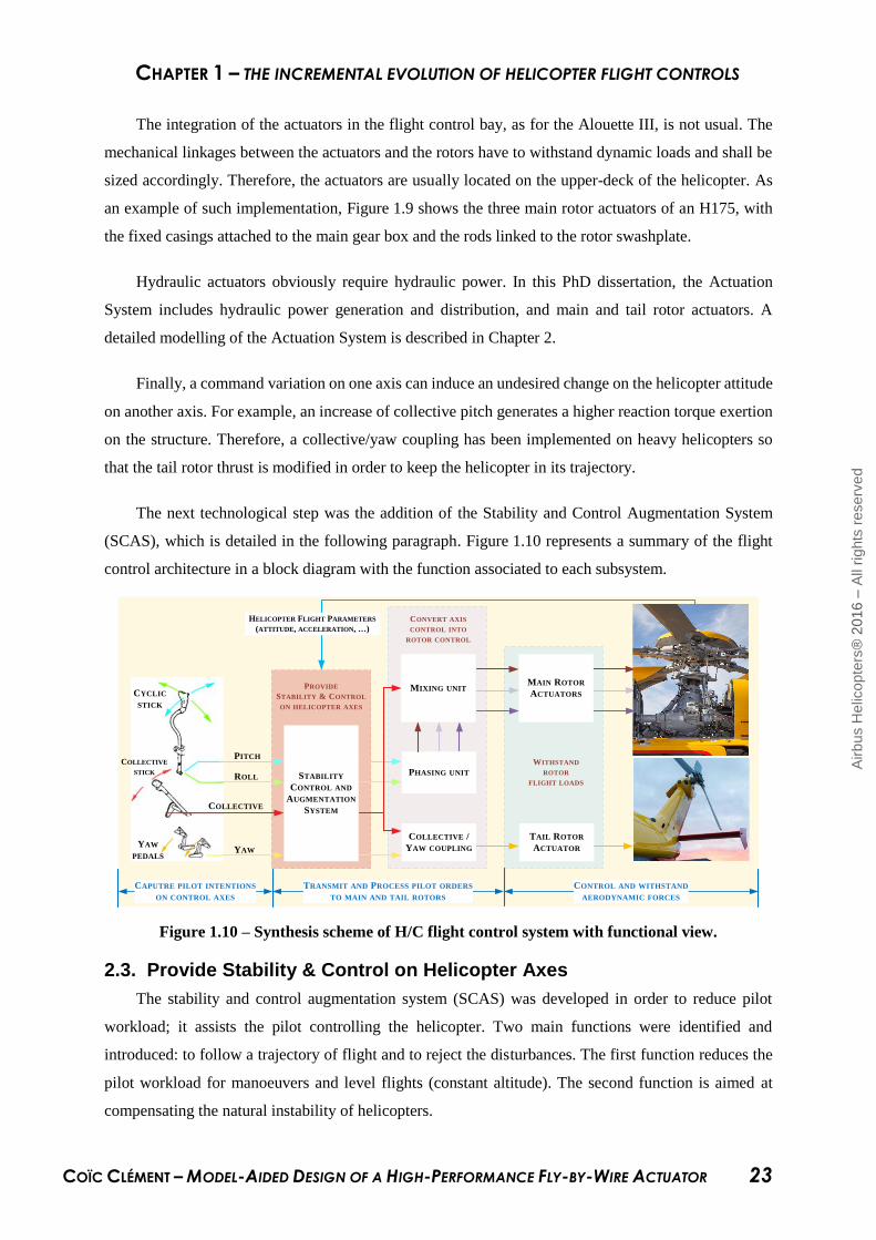
The next technological step was the addition of the Stability and Control Augmentation System
(SCAS), which is detailed in the following paragraph. Figure 1.10 represents a summary of the flight
control architecture in a block diagram with the function associated to each subsystem.
CYCLIC
STICK
COLLECTIVE
STICK
YAW
PEDALS
PITCH
ROLL
COLLECTIVE
YAW
STABILITY
CONTROL AND
AUGMENTATION
SYSTEM
COLLECTIVE /
YAW COUPLING
PHASING UNIT
MAIN ROTOR
ACTUATORS
TAIL ROTOR
ACTUATOR
CAPUTRE PILOT INTENTIONS
ON CONTROL AXES
TRANSMIT AND PROCESS PILOT ORDERS
TO MAIN AND TAIL ROTORS
CONTROL AND WITHSTAND
AERODYNAMIC FORCES
PROVIDE
STABILITY & CONTROL
ON HELICOPTER AXES
WITHSTAND
ROTOR
FLIGHT LOADS
HELICOPTER FLIGHT PARAMETERS
(ATTITUDE, ACCELERATION, …)
MIXING UNIT
CONVERT AXIS
CONTROL INTO
ROTOR CONTROL
Figure 1.10 – Synthesis scheme of H/C flight control system with functional view.
2.3. Provide Stability & Control on Helicopter Axes
The stability and control augmentation system (SCAS) was developed in order to reduce pilot
workload; it assists the pilot controlling the helicopter. Two main functions were identified and
introduced: to follow a trajectory of flight and to reject the disturbances. The first function reduces the
pilot workload for manoeuvers and level flights (constant altitude). The second function is aimed at
compensating the natural instability of helicopters.
Airb
us H
elic
opte
rs®
2016 –
All
rights
reserv
ed

CHAPTER 1 – THE INCREMENTAL EVOLUTION OF HELICOPTER FLIGHT CONTROLS
COÏC CLÉMENT – MODEL-AIDED DESIGN OF A HIGH-PERFORMANCE FLY-BY-WIRE ACTUATOR 24
For these needs, SCAS actuators are integrated in almost all medium and heavy helicopters. Two
main principles are used on the conventional flight control system:
Added motion in series with the pilot input. This motion is not perceived by the pilot. Actuators
in series usually generate high speed and high bandwidth SCAS orders with limited authority. In
comparison with pilot orders, their maximum amplitudes are low. They are mainly used for
stabilization. This function is usually realized with one of the following solutions:
1. Smart Electro Mechanical Actuators (SEMA): These actuators were originally called serial
actuators. They integrate electronic hardware and are controlled by a digital signal
(Figure 1.11).
2. Automatic Stabilization Equipment (ASE): This equipment was first introduced on the
Sikorsky S55. In some designs, the flight control kinematic friction is too high regarding the
SEMA capabilities. ASE then fulfils this function with the help of hydraulic power
(Figure 1.12).
Figure 1.11 – SEMA. Figure 1.12 – ASE [webSITEC].
Added motion in parallel with the pilot input. In this case the stick moves in the same proportion
as the autopilot order. TRIM actuators (Figure 1.13) ensure this function. They have low speed
but full authority on the pilot command. They can be used either by the pilot to hold a position
order without effort, or by the autopilot to re-centre the SEMAs in order to keep a symmetrical
margin of travel.
Figure 1.13 – Trim actuator. Figure 1.14 – SCAS actuation concept.
Airb
us H
elic
opte
rs®
2016 –
All
rights
reserv
ed

CHAPTER 1 – THE INCREMENTAL EVOLUTION OF HELICOPTER FLIGHT CONTROLS
COÏC CLÉMENT – MODEL-AIDED DESIGN OF A HIGH-PERFORMANCE FLY-BY-WIRE ACTUATOR 25
Figure 1.14 is a simple representation of both series and parallel actuators in the conventional flight
control system and their impact on the blade pitch.
The control of the SCAS actuators is made possible by the Automatic Flight Control System
(AFCS) computer called Auto-Pilot Module (APM) at Airbus Helicopters. It receives helicopters flight
parameters from dedicated sensors to generate the series and parallel actuator commands. The criticality
associated to this equipment, if the helicopter is naturally aerodynamically stable, is “major” as defined
in Table 1.1 taken from [SAE96].
Table 1.1: Failure condition severity taken from [SAE96].
This table regroups the qualitative and quantitative probability of failure per flight hour for both
the Federal Aviation Administration (FAA) and the Joint Aviation Authorities (JAA – that preceded the
European Aviation Safety Agency (EASA) now the European reference for aviation safety).
2.4. Withstand Rotor Flight Loads – Hydro-Mechanical Actuators
2.4.1. Generic Hydraulic Actuator
The hydraulic actuators are inserted in the flight control kinematics in order to implement the pilot
orders and provide hydraulic assistance to face the aerodynamic loads. The force to be applied by the
pilot to the stick should not exceed 0.25 daN in nominal operation. In contrast, within the flight domain,
the aerodynamic load that is reflected to one main rotor actuator of a medium helicopter such as the
AS365 can reach up to 300 daN [MARG11]. These static and dynamic loads can be much higher for
heavier rotorcraft such as the H225 or NH90.
Airb
us H
elic
opte
rs®
2016 –
All
rights
reserv
ed

CHAPTER 1 – THE INCREMENTAL EVOLUTION OF HELICOPTER FLIGHT CONTROLS
COÏC CLÉMENT – MODEL-AIDED DESIGN OF A HIGH-PERFORMANCE FLY-BY-WIRE ACTUATOR 26
In order to keep a normalized vocabulary throughout this PhD dissertation, a generic hydraulic
actuator is introduced with a word Bond-graph in Figure 1.15. The Bond-graph formalism is introduced
in Chapter 1. However, some conventions shall be explained in advance. Half arrows (bonds) transmit
power, while complete arrows stand for signals. Dashed lines are optional power/signal paths. The
colour denotes the physical domain (here: blue for hydraulics, green for mechanics and black for a non-
defined domain depending on the chosen technology). This representation makes the order of magnitude
of the involved variables perceptible: pilots provide mechanically signalled commands and actuator
output is mechanical power. This coincides with the orders of magnitude given at the beginning of this
section. The functions fulfilled by the subsystems are the following:
The interface stage: to receive the input signals and transmit them to the pilot stage.
The pilot stage: to drive the power modulation stage based on the output of the interface stage.
The power modulation stage: to receive the hydraulic power supply and to modulate it to
provide flow and pressure to the cylinder.
The cylinder: to receive the modulated hydraulic power and transform it into mechanical power.
The closed-loop: to control the actuator movement versus the input signals. Helicopter flight
control actuators are position-controlled.
ACTUATOR
INPUTOUTPUTPILOT
STAGE
POWER
MODULATION
STAGE
CYLINDERCLOSED
LOOP
INTERFACE
STAGE
CONTROL MODULE
HYDRAULIC
POWER SUPPLY
Figure 1.15 – Actuator word Bond-graphs from [COI15b].
2.4.2. Actuator Architecture Driven by Response to Failure
As the flight control system is a safety-critical function, response to failure drives the architecture
of aerospace actuators. This section introduces some general safety requirement impacts on actuators
and their consequences for a hydro-mechanical actuator.
2.4.2.1. Generalities
“The rotorcraft systems and associated components, considered separately and in relation to other
systems, must be designed so that (…) the occurrence of any failure condition which would prevent the
Airb
us H
elic
opte
rs®
2016 –
All
rights
reserv
ed

CHAPTER 1 – THE INCREMENTAL EVOLUTION OF HELICOPTER FLIGHT CONTROLS
COÏC CLÉMENT – MODEL-AIDED DESIGN OF A HIGH-PERFORMANCE FLY-BY-WIRE ACTUATOR 27
continued safe flight and landing of the rotorcraft is extremely improbable” JAR 29.1309-(b)-(2)-(i)
[JAA99].
Safety requirements are legitimate for the flight control system as it ensures a critical function on
the helicopter. Loss of the helicopter control leads to the loss of the rotorcraft. Therefore, the architecture
of the flight control system components is highly impacted by these requirements.
Subpart (c) of paragraph §695 in the main certification regulations (FAR 29 [FAA65] and CS29
[EAS07] for heavy helicopters) states that “the failure of mechanical parts (such as piston rods and
links), and the jamming of power cylinders, must be considered unless they are extremely improbable”1.
A correct sizing including stress and fatigue analyses with the right safety coefficients enables
considering one single mechanical path for the flight control system (safe-life).
However, hydraulic and electrical individual faults and failures are not extremely improbable and
shall thus always be considered in actuator architecture and design. It is also important to note that the
jamming of the power modulation stage is not covered by paragraph §695 – (c). The actuator’s
architecture and design shall meet the safety objectives with respect to its own failure and possible cross
failures with external events. Typically, external events that shall be considered in an actuator
development are [COI14]:
Loss of the hydraulic power supply. There can be multiple root causes: pump failure, pipe
disconnection or rupture…
Malfunction of the hydraulic power supply. For example, an increase of pump internal leakage
leading to a decrease in pressure supply.
Loss of the electrical input signal (in case of FbW flight controls). This could be due to the loss
of one Flight Control Processing (FCP) or a cable disconnection.
Erroneous electrical input signal (if FbW), e.g. malfunction of the FCP.
1 The terms probable, improbable, extremely improbable or frequent, reasonably probable, remote, extremely
remote, and extremely improbable relate to probability objectives [SAE96].
Airb
us H
elic
opte
rs®
2016 –
All
rights
reserv
ed

CHAPTER 1 – THE INCREMENTAL EVOLUTION OF HELICOPTER FLIGHT CONTROLS
COÏC CLÉMENT – MODEL-AIDED DESIGN OF A HIGH-PERFORMANCE FLY-BY-WIRE ACTUATOR 28
Figure 1.16 – System response to component failure [MAR16].
Figure 1.16 synthesizes the different manners in which a system can respond to a failure. Based on
this terminology, actuator design shall be fail-active so the overall flight control system function is
ensured. While satisfying this condition, redundant subsystems of the actuator can be fail-safe.
Once these generalities have been introduced, Figure 1.15 appears to be a simplification of the
possible architecture for helicopter actuators. Redundancies are not represented: they include multiple
interface and pilot stages, usually two (even three for the Bell 525 Relentless) power modulation stages
and jacks. Passivation elements needed to avoid catastrophic response to failure are not shown either.
The choice has been made to introduce such generic architecture so that each kind of actuator studied
within the scope of this dissertation could fit to it. Specificities of each technology, mostly related to its
response to failures, will be detailed in a dedicated part of this chapter.
2.4.2.2. Hydro-Mechanical Actuator
In conventional flight controls, pilot commands are transmitted to the actuators through a single
path2 of mechanical links (safe-life). The interface stage is thus usually a mechanical lever, the kinematic
linkage of which corresponds to the pilot stage. Action on the lever induces a displacement of the control
valve (power modulation stage) to feed the hydraulic cylinder.
Valve jamming is extremely remote, but not extremely improbable. Therefore, a back-up spool
(usually a concentric second valve) is integrated on the power modulation stage. Also, the loss of one
hydraulic circuit is an external event that shall be considered. Therefore, two segregated hydraulic
circuits are usually implemented. The power modulation stage and the cylinder are thus duplicated.
Should a hydraulic circuit loss occur, the cylinder concerned will respond in a fail-passive way. The
2 Military helicopters can have two segregated paths of mechanical links in order to reduce the vulnerability to
bullets. This is for example the case on the Sikorsky S-92.
Airb
us H
elic
opte
rs®
2016 –
All
rights
reserv
ed
CHAPTER 1 – THE INCREMENTAL EVOLUTION OF HELICOPTER FLIGHT CONTROLS
COÏC CLÉMENT – MODEL-AIDED DESIGN OF A HIGH-PERFORMANCE FLY-BY-WIRE ACTUATOR 29
second cylinder enables the actuator to remain fail-operative or fail-functional depending on the design
choices.
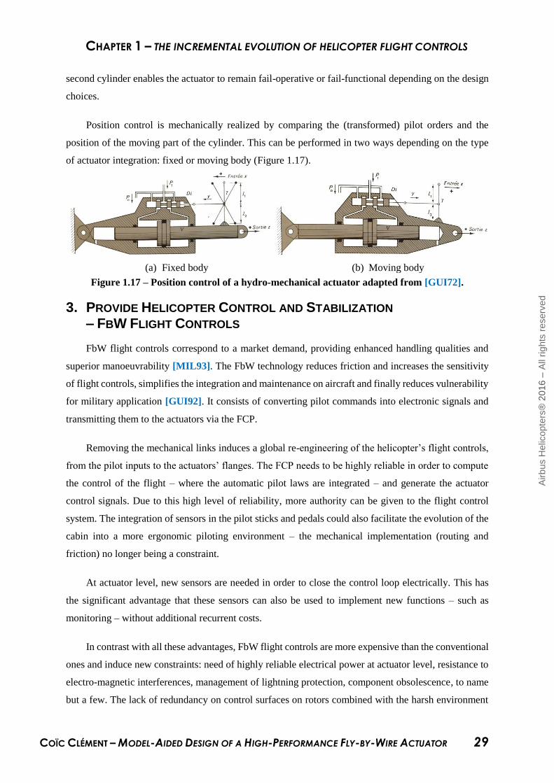
Position control is mechanically realized by comparing the (transformed) pilot orders and the
position of the moving part of the cylinder. This can be performed in two ways depending on the type
of actuator integration: fixed or moving body (Figure 1.17).
(a) Fixed body (b) Moving body
Figure 1.17 – Position control of a hydro-mechanical actuator adapted from [GUI72].
3. PROVIDE HELICOPTER CONTROL AND STABILIZATION – FBW FLIGHT CONTROLS
FbW flight controls correspond to a market demand, providing enhanced handling qualities and
superior manoeuvrability [MIL93]. The FbW technology reduces friction and increases the sensitivity
of flight controls, simplifies the integration and maintenance on aircraft and finally reduces vulnerability
for military application [GUI92]. It consists of converting pilot commands into electronic signals and
transmitting them to the actuators via the FCP.
Removing the mechanical links induces a global re-engineering of the helicopter’s flight controls,
from the pilot inputs to the actuators’ flanges. The FCP needs to be highly reliable in order to compute
the control of the flight – where the automatic pilot laws are integrated – and generate the actuator
control signals. Due to this high level of reliability, more authority can be given to the flight control
system. The integration of sensors in the pilot sticks and pedals could also facilitate the evolution of the
cabin into a more ergonomic piloting environment – the mechanical implementation (routing and
friction) no longer being a constraint.
At actuator level, new sensors are needed in order to close the control loop electrically. This has
the significant advantage that these sensors can also be used to implement new functions – such as
monitoring – without additional recurrent costs.
In contrast with all these advantages, FbW flight controls are more expensive than the conventional
ones and induce new constraints: need of highly reliable electrical power at actuator level, resistance to
electro-magnetic interferences, management of lightning protection, component obsolescence, to name
but a few. The lack of redundancy on control surfaces on rotors combined with the harsh environment
Airb
us H
elic
opte
rs®
2016 –
All
rights
reserv
ed
CHAPTER 1 – THE INCREMENTAL EVOLUTION OF HELICOPTER FLIGHT CONTROLS
COÏC CLÉMENT – MODEL-AIDED DESIGN OF A HIGH-PERFORMANCE FLY-BY-WIRE ACTUATOR 30
(vibrations, high temperature, etc.) make the implementation of FbW more complex and more risky on
helicopters than on fixed wings. This explains why commercial airplanes have integrated FbW flight
controls since the late 1960s (Concorde) but only a single rotorcraft (NH90) has been produced in series
with this technology since 2006.
The trade-off between mechanical and FbW flight controls reveals many advantages and
disadvantages for both technologies. The chosen solution may differ from one helicopter to another,
according to the customers’ needs or the market target.
3.1. Capture Pilot Intentions on Control Axes
FbW flight controls do not necessarily modify the pilot’s control interfaces: sticks and pedals can
remain unchanged. However, new opportunities are introduced as sensitivity of command can be
managed electrically. As an example, mini-sticks are tested in combination with FbW flight control
systems [SED89] to improve piloting ergonomics.
Also, the removal of mechanical linkages enables the implementation of new flight control laws.
One concrete example would be the advanced control laws in which pilot input (stick or pedal deflection)
is directly translated into piloting objectives such as helicopter attitudes (e.g. pitch angle, bank angle,
heading, etc.).
3.2. Transmit Pilots Orders to Main and Tail Rotors
Pilot intentions, once converted into electrical signals by means of the sensors, are transmitted to
the FCPs. In case of conventional flight laws, the FCPs perform the same functions as conventional
flight controls (control gain, mixing, coupling and phasing), as detailed in section 2.
Implementation of complex mechanical components such as phasing units is easily performed in
an FCP: it is only a change of reference frame, i.e. a matrix. Therefore, the integration of the actuators
around the main gear box is less constrained and weight can be minimized at system level with low
implementation costs.
Particular attention is required when developing an FCP. It is indeed a key component of the flight
control system as all orders transit through it. The right level of redundancy and dissimilarity has to be
selected in order to meet the safety requirements of the entire flight control system.
3.3. Provide Stability & Control on Helicopter Axes
As detailed at the beginning of section 3, one of the main advantages of FbW flight control systems
is the extremely high reliability of the FCPs. This allows implementing stabilization and control
functions at any time of the flight and after any failure combination, occurrence of which is extremely
improbable. Such new functions can be added at FCP level without the need of additional actuators.
Airb
us H
elic
opte
rs®
2016 –
All
rights
reserv
ed
CHAPTER 1 – THE INCREMENTAL EVOLUTION OF HELICOPTER FLIGHT CONTROLS
COÏC CLÉMENT – MODEL-AIDED DESIGN OF A HIGH-PERFORMANCE FLY-BY-WIRE ACTUATOR 31
Serial actuation (SEMA or ASE) is thus no longer required, which reduces weight and increases overall
flight control system reliability. The parallel actuation (Trims) remains unchanged as there is still a need
for moving the inceptors to provide information on the actuator position to the pilot in case of
conventional sticks (it is no longer needed for mini-sticks).
3.4. Withstand Rotor Flight Loads – FbW Actuators
When the FbW flight control system is implemented, the actuator input is no longer mechanical
but performed by electrical signals. Therefore, actuator control modules need to integrate interface
stages able to receive these signals. The position closed loop requires position sensors at jack level. The
control signal is generated by the Actuator Control Loop (ACL).
Initially, FbW actuators were developed for military needs – fighter aircraft, radar drives, guidance
platform drives, controls for missile launchers and spaceships – using Electro-Hydraulic ServoValves
(EHSV) as an interface between the signal and the hydraulic power domains: the control module. EHSV
provides high power gains – on the order of 104 to 106 – with low command currents – less than ±40 mA
for the industry and usually ±8 mA for aeronautic applications [MAS78].
However, the use of the EHSV technology on helicopters is not trivial. Performances at low
temperature, reliability in a vibrating environment, response to failure and hydraulic continuous power
consumption are its main challenges.
With the arrival of the electrical power generation system on aircraft for many uses such as air
conditioning, a new technology has become a reference in flight controls for piloting a jack: the Direct
Drive Valve (DDV). The use of a DDV as a control module removes the drawbacks listed for the EHSV.
On the other hand, it requires more electrical power: around 50 Watt in demanding configurations such
as jamming issues.
These two technologies are described in this chapter as they represent opportunities for FbW flight
controls on helicopters. Recommendations on their implementation perimeter are provided at the end of
this part.
3.4.1. EHSV-Based Actuators
3.4.1.1. Control Module
The EHSV uses one or several motors (also referred to as coils by convention) as interface stage
which receive a current as input. They act on a hydraulic potentiometer (pilot stage) that displaces the
valve proportionally (power modulation stage). This combination of electric signal with a hydraulic
potentiometer is at the origin of the term “electro-hydraulic” for the servovalves.
Airb
us H
elic
opte
rs®
2016 –
All
rights
reserv
ed
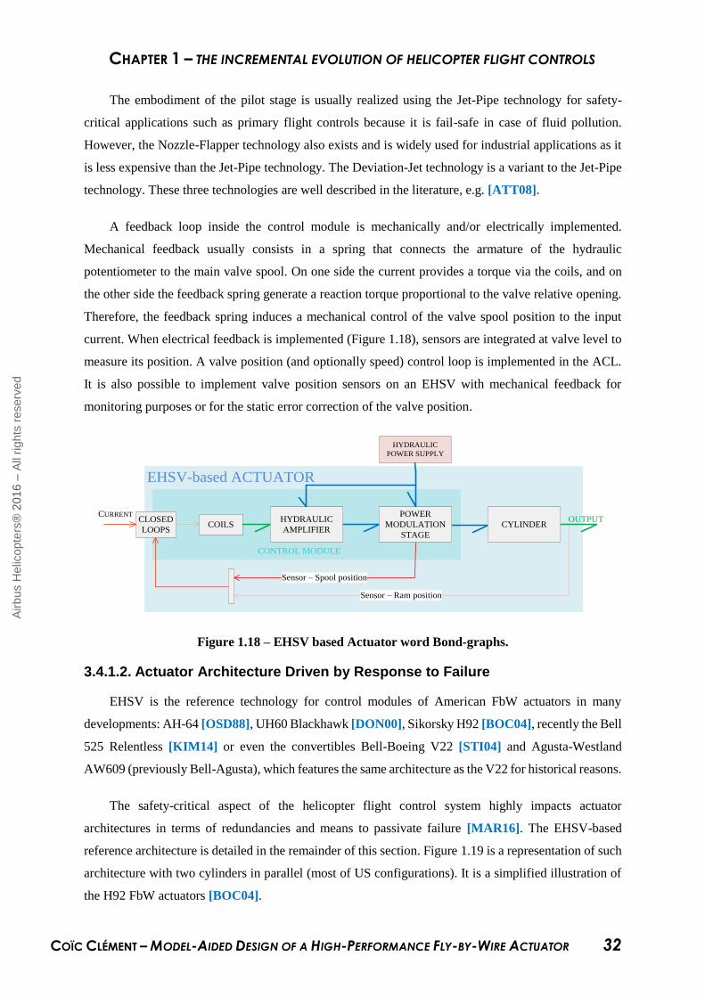
CHAPTER 1 – THE INCREMENTAL EVOLUTION OF HELICOPTER FLIGHT CONTROLS
COÏC CLÉMENT – MODEL-AIDED DESIGN OF A HIGH-PERFORMANCE FLY-BY-WIRE ACTUATOR 32
The embodiment of the pilot stage is usually realized using the Jet-Pipe technology for safety-
critical applications such as primary flight controls because it is fail-safe in case of fluid pollution.
However, the Nozzle-Flapper technology also exists and is widely used for industrial applications as it
is less expensive than the Jet-Pipe technology. The Deviation-Jet technology is a variant to the Jet-Pipe
technology. These three technologies are well described in the literature, e.g. [ATT08].
A feedback loop inside the control module is mechanically and/or electrically implemented.
Mechanical feedback usually consists in a spring that connects the armature of the hydraulic
potentiometer to the main valve spool. On one side the current provides a torque via the coils, and on
the other side the feedback spring generate a reaction torque proportional to the valve relative opening.
Therefore, the feedback spring induces a mechanical control of the valve spool position to the input
current. When electrical feedback is implemented (Figure 1.18), sensors are integrated at valve level to
measure its position. A valve position (and optionally speed) control loop is implemented in the ACL.
It is also possible to implement valve position sensors on an EHSV with mechanical feedback for
monitoring purposes or for the static error correction of the valve position.
EHSV-based ACTUATOR
CONTROL MODULE
Sensor – Ram position
CURRENTOUTPUT
HYDRAULIC
POWER SUPPLY
Sensor – Spool position
HYDRAULIC
AMPLIFIER
POWER
MODULATION
STAGE
CYLINDERCLOSED
LOOPSCOILS
Figure 1.18 – EHSV based Actuator word Bond-graphs.
3.4.1.2. Actuator Architecture Driven by Response to Failure
EHSV is the reference technology for control modules of American FbW actuators in many
developments: AH-64 [OSD88], UH60 Blackhawk [DON00], Sikorsky H92 [BOC04], recently the Bell
525 Relentless [KIM14] or even the convertibles Bell-Boeing V22 [STI04] and Agusta-Westland
AW609 (previously Bell-Agusta), which features the same architecture as the V22 for historical reasons.
The safety-critical aspect of the helicopter flight control system highly impacts actuator
architectures in terms of redundancies and means to passivate failure [MAR16]. The EHSV-based
reference architecture is detailed in the remainder of this section. Figure 1.19 is a representation of such
architecture with two cylinders in parallel (most of US configurations). It is a simplified illustration of
the H92 FbW actuators [BOC04].
Airb
us H
elic
opte
rs®
2016 –
All
rights
reserv
ed

CHAPTER 1 – THE INCREMENTAL EVOLUTION OF HELICOPTER FLIGHT CONTROLS
COÏC CLÉMENT – MODEL-AIDED DESIGN OF A HIGH-PERFORMANCE FLY-BY-WIRE ACTUATOR 33
The EHSV-based reference architecture includes 2 (or even 3) segregated hydraulic circuits. Each
of them supplies a control module that provides power to a cylinder. Both power outputs of the cylinder
rod are mechanically linked by an attachment fitting, which adds up the forces.
Figure 1.19 – EHSV based reference actuator.
Each control module includes a three-coil jet-pipe electro-hydraulic servovalve with mechanical
feedback and sensors to monitor their main valve. Coil redundancy ensures that the generated torque
remains sufficient (fail-operative) after the loss of one coil (or the loss of its command) and that degraded
performances (fail-functional) after the loss of two coils remain acceptable. The three-coil design also
enables the implementation of a monitoring strategy by comparison of the three currents. Finally, the
risk of rupture of the feedback spring or valve jamming requires the addition of a by-pass valve between
the control modules and the cylinders. The position of the by-pass is also monitored to prevent a dormant
failure (jamming in open position). It is important to note that, unlike in hydro-mechanical actuators,
the back-up spool solution to valve jamming is not implemented due to its integration complexity.
Pressure difference sensors are necessary to synchronise both servovalves. Both valves need to
open at the same time, in the same proportion and in the same direction to avoid generating force-
fighting at cylinder level.
This description is bottom-up, deducing the requirements from an existing design. However, the
first designs were top-down approaches based on flight control system requirements and safety analysis
support. It has been decided not to detail the safety analyses in this dissertation as they are realized by a
3-coils EHSV
Airb
us H
elic
opte
rs®
2016 –
All
rights
reserv
ed

CHAPTER 1 – THE INCREMENTAL EVOLUTION OF HELICOPTER FLIGHT CONTROLS
COÏC CLÉMENT – MODEL-AIDED DESIGN OF A HIGH-PERFORMANCE FLY-BY-WIRE ACTUATOR 34
dedicated department at Airbus Helicopters. Candidate architectures shall meet the safety requirements.
The aim is to ensure that single failure or failure combinations leading to the loss of the function are
extremely improbable for safety-critical functions such as the flight control system. Tools such as Fault
Tree Analysis (FTA) are used to validate this safety requirement.
3.4.1.3. Advantages and Disadvantages with Respect to Helicopter Application
Typically, the MIL-PRF-83282 can be used as hydraulic fluid for helicopters. Its operating
temperature ranges from -40°C to +205°C [SAE00]. The associated variation of oil properties negatively
impacts the actuator and hydraulic circuit sizing and, consequently, mass. Therefore, the embedded
power system suffers severe environmental and power consumption constraints. Also, it is relevant to
consider cost constraints in order to ensure economic viability of the product.
The advantages and disadvantages of the EHSV technology are multiple but it has been decided to
focus on those who affect the three criteria listed above.
Main advantages selected:
1. Low electrical power consumption. For a typical servovalve used for aerospace application, a
±7.5 mA input current through a coil resistance of 400 Ω (the maximum electrical power is
22,5 mW) can control a flow of up to 150 L/min with a differential pressure of 200 Bar (the
maximum hydraulic power is 50 kW). The hydraulic/electrical power ratio is 2.106 [FAI83].
2. Low sensitivity to pollution of the power modulation stage. For a spool with a 4.62 mm diameter
[MOO87] and a hydraulic power supply set at 206 Bar, the chip shear force – the capability to
“cut” a particle blocking the valve – is up to 345 N.
3. Off-the-shelf parts. EHSV are well established as a reference component for aerospace and
industrial actuators. The cost of off-the-shelf equipment is reduced compared to specific
equipment.
4. EHSV with internal mechanical feedback requires only one ram position closed loop. This
requires lower processing frequencies at ACL level in case of digital implementation.
Main drawbacks selected:
1. High hydraulic power consumption. Typically, the pilot stage consumes a permanent 0.5 L/min
flow for a new EHSV and could reach 1.5 L/min at end of life. This corresponds to a power
dissipation between 170 W and 500 W for a 206 Bar supply pressure. Considering two
servovalves per actuator and four actuators per helicopter, power dissipation of the pilot stage can
be up to 4 kW at helicopter level.
2. High sensitivity to fluid pollution of the pilot stage. In order to reduce the operating flow, pilot
stages use very small hydraulic restrictions. These restrictions make the EHSV sensitive to fluid
pollution. This effect is supposed to be minimized by the jet pipe technology, as it only introduces
Airb
us H
elic
opte
rs®
2016 –
All
rights
reserv
ed
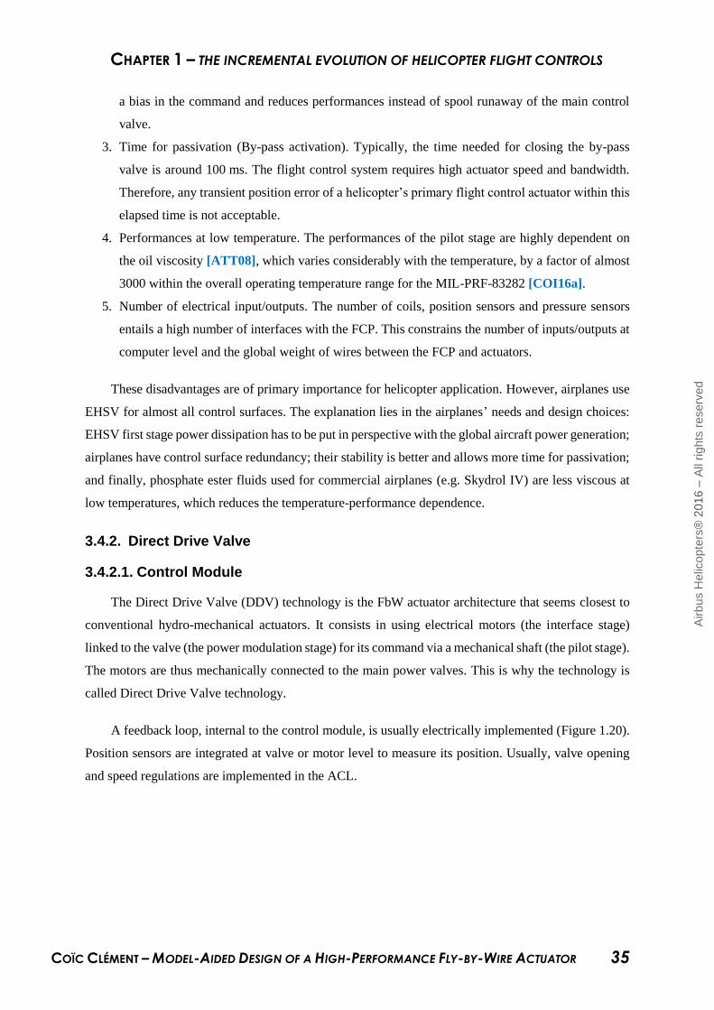
CHAPTER 1 – THE INCREMENTAL EVOLUTION OF HELICOPTER FLIGHT CONTROLS
COÏC CLÉMENT – MODEL-AIDED DESIGN OF A HIGH-PERFORMANCE FLY-BY-WIRE ACTUATOR 35
a bias in the command and reduces performances instead of spool runaway of the main control
valve.
3. Time for passivation (By-pass activation). Typically, the time needed for closing the by-pass
valve is around 100 ms. The flight control system requires high actuator speed and bandwidth.
Therefore, any transient position error of a helicopter’s primary flight control actuator within this
elapsed time is not acceptable.
4. Performances at low temperature. The performances of the pilot stage are highly dependent on
the oil viscosity [ATT08], which varies considerably with the temperature, by a factor of almost
3000 within the overall operating temperature range for the MIL-PRF-83282 [COI16a].
5. Number of electrical input/outputs. The number of coils, position sensors and pressure sensors
entails a high number of interfaces with the FCP. This constrains the number of inputs/outputs at
computer level and the global weight of wires between the FCP and actuators.
These disadvantages are of primary importance for helicopter application. However, airplanes use
EHSV for almost all control surfaces. The explanation lies in the airplanes’ needs and design choices:
EHSV first stage power dissipation has to be put in perspective with the global aircraft power generation;
airplanes have control surface redundancy; their stability is better and allows more time for passivation;
and finally, phosphate ester fluids used for commercial airplanes (e.g. Skydrol IV) are less viscous at
low temperatures, which reduces the temperature-performance dependence.
3.4.2. Direct Drive Valve
3.4.2.1. Control Module
The Direct Drive Valve (DDV) technology is the FbW actuator architecture that seems closest to
conventional hydro-mechanical actuators. It consists in using electrical motors (the interface stage)
linked to the valve (the power modulation stage) for its command via a mechanical shaft (the pilot stage).
The motors are thus mechanically connected to the main power valves. This is why the technology is
called Direct Drive Valve technology.
A feedback loop, internal to the control module, is usually electrically implemented (Figure 1.20).
Position sensors are integrated at valve or motor level to measure its position. Usually, valve opening
and speed regulations are implemented in the ACL.
Airb
us H
elic
opte
rs®
2016 –
All
rights
reserv
ed
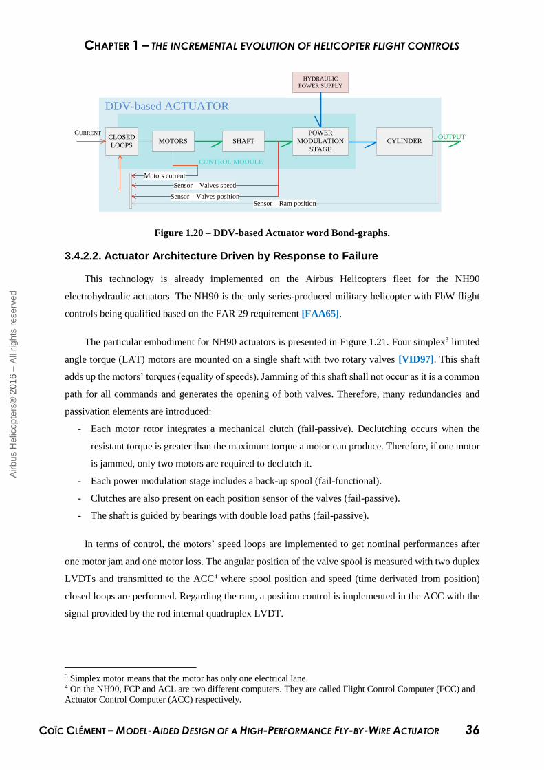
CHAPTER 1 – THE INCREMENTAL EVOLUTION OF HELICOPTER FLIGHT CONTROLS
COÏC CLÉMENT – MODEL-AIDED DESIGN OF A HIGH-PERFORMANCE FLY-BY-WIRE ACTUATOR 36
DDV-based ACTUATOR
CONTROL MODULE
Sensor – Ram position
CURRENTOUTPUT
HYDRAULIC
POWER SUPPLY
Sensor – Valves position
CYLINDERMOTORS SHAFT
POWER
MODULATION
STAGE
Sensor – Valves speed
Motors current
CLOSED
LOOPS
Figure 1.20 – DDV-based Actuator word Bond-graphs.
3.4.2.2. Actuator Architecture Driven by Response to Failure
This technology is already implemented on the Airbus Helicopters fleet for the NH90
electrohydraulic actuators. The NH90 is the only series-produced military helicopter with FbW flight
controls being qualified based on the FAR 29 requirement [FAA65].
The particular embodiment for NH90 actuators is presented in Figure 1.21. Four simplex3 limited
angle torque (LAT) motors are mounted on a single shaft with two rotary valves [VID97]. This shaft
adds up the motors’ torques (equality of speeds). Jamming of this shaft shall not occur as it is a common
path for all commands and generates the opening of both valves. Therefore, many redundancies and
passivation elements are introduced:
- Each motor rotor integrates a mechanical clutch (fail-passive). Declutching occurs when the
resistant torque is greater than the maximum torque a motor can produce. Therefore, if one motor
is jammed, only two motors are required to declutch it.
- Each power modulation stage includes a back-up spool (fail-functional).
- Clutches are also present on each position sensor of the valves (fail-passive).
- The shaft is guided by bearings with double load paths (fail-passive).
In terms of control, the motors’ speed loops are implemented to get nominal performances after
one motor jam and one motor loss. The angular position of the valve spool is measured with two duplex
LVDTs and transmitted to the ACC4 where spool position and speed (time derivated from position)
closed loops are performed. Regarding the ram, a position control is implemented in the ACC with the
signal provided by the rod internal quadruplex LVDT.
3 Simplex motor means that the motor has only one electrical lane. 4 On the NH90, FCP and ACL are two different computers. They are called Flight Control Computer (FCC) and
Actuator Control Computer (ACC) respectively.
Airb
us H
elic
opte
rs®
2016 –
All
rights
reserv
ed

CHAPTER 1 – THE INCREMENTAL EVOLUTION OF HELICOPTER FLIGHT CONTROLS
COÏC CLÉMENT – MODEL-AIDED DESIGN OF A HIGH-PERFORMANCE FLY-BY-WIRE ACTUATOR 37
P1 P2
R1
Hydraulic System 2Hydraulic System 1
R2
LVDT DUPLEXLVDT DUPLEX
4 Torque
motors
Valves
Hydraulic System 1
Valves
Hydraulic System 2
LVDT QUADRUPLEX
Figure 1.21 – NH90 Direct Drive Valve actuator.
The valves are mechanically synchronised by a precise positioning of the valves on the shaft to
prevent force fight of the two actuator cylinders, as is the case for hydro-mechanical actuators.
3.4.2.3. Advantages and Disadvantages with Respect to Helicopter Application
With the same approach as for the EHSV, advantages and disadvantages of the DDV technology
based on environmental, power consumption and cost constraints are listed in the following paragraph.
Main advantages selected:
1. Low transients after failure. The high stiffness and bandwidth of the motors’ speed loop ensure a
quick declutching in case of jamming.
2. Hydraulic and electric failure decoupling. The pilot stage (the shaft) is unique. This means that
any interface stage can control both power modulation stages. For example, after a hydraulic
circuit loss, the four motors still pilot – through the shaft – the valve associated with the remaining
hydraulic power source. Also, such failure decoupling allows a take-off after the loss of one
electrical lane as the three remaining motors can still pilot both main power valves.
3. No permanent operating flow and thus temperature-related performance of the pilot stage. The
shaft drives the power modulation stages from the output of the interface stages. Such technical
solution is almost insensitive to temperature variation and does not require any hydraulic supply.
4. Lighter technology. The weight of the motors is not in favour of the DDV solution, but as this
technology does not need any further passivation components (e.g. by-pass valve) or pressure
sensors, the global weight is lower than an EHSV-based actuator.
Airb
us H
elic
opte
rs®
2016 –
All
rights
reserv
ed

CHAPTER 1 – THE INCREMENTAL EVOLUTION OF HELICOPTER FLIGHT CONTROLS
COÏC CLÉMENT – MODEL-AIDED DESIGN OF A HIGH-PERFORMANCE FLY-BY-WIRE ACTUATOR 38
Main drawbacks selected:
1. Higher electrical consumption. Few amperes are needed for declutching. However, even if
nominal power consumption is approximately 50 times smaller than declutching power, it is still
20 times higher than EHSV nominal power.
2. Control complexity inside the ACC. The DDV technology requires four control loops, as detailed
in section 3.4.2.1. Each inner loop requires a higher bandwidth than the outer loop. Therefore, the
current loops require several kilo-Hertz of bandwidth and thus an even higher sampling rate.
Implementation of digital ACC becomes therefore more complex.
In addition to these points, Airbus Helicopters is familiar with this technology. A new development
could be easier with a DDV-based actuator thanks to the experience acquired during NH90 development
and service feedback. Benefits should be notable on development cost and schedule.
3.4.3. Technology Recommendation
In accordance with the arguments given above, this dissertation recommends using the DDV
technology for primary flight control actuators on FbW helicopters for safety aspects, weight savings
and performances at low temperatures5. Customer satisfaction is Airbus Helicopters’ top priority and
these points are all linked to this goal.
Nevertheless, the EHSV technology is well suited for functions with lower criticality. Secondary
flight controls with low authority could be concerned. For a function on which failure is probable, the
actuator architecture using a single hydraulic cylinder would be simplified and implementation with an
EHSV-based control module would be easier.
5 A safety-critical function, such as the flight control system, shall not be downsized.
Airb
us H
elic
opte
rs®
2016 –
All
rights
reserv
ed

CHAPTER 1 – THE INCREMENTAL EVOLUTION OF HELICOPTER FLIGHT CONTROLS
COÏC CLÉMENT – MODEL-AIDED DESIGN OF A HIGH-PERFORMANCE FLY-BY-WIRE ACTUATOR 39
4. FUTURE OF HELICOPTERS FLIGHT CONTROLS
It has been chosen to present a selection of previous and current works for their potential to improve
helicopter flight controls.
4.1. FbW Retrofit – SIA
A recent technology – the Smart Interface Actuator (SIA) – has been recently patented [GRO13]
and investigated by Pierre Estival within the scope of his PhD research [EST15] at Airbus Helicopters.
The SIA is a position-controlled electro-mechanical actuator. It pilots the mechanical lever of a hydro-
mechanical actuator which has its own mechanical position control loop.
OUTPUT
SMART INTERFACE ACTUATORHYDRO-MECHANICAL
ACTUATORSHORT
KINEMATICINPUT
Figure 1.22 – SIA concept, in series with a conventional actuator.
This technology seems well suited for retrofitting conventional helicopters to equip them with FbW
flight control systems. In fact, as the effort needed to move the input lever of a conventional actuator
and the lever stroke are similar for all Airbus Helicopters fleet, only one SIA could be developed and
fitted to the entire fleet retrofit. Helicopters with conventional flight controls could be upgraded with
FbW flight controls at low development cost.
This technology suffers from a lack of maturity but could be very promising if efforts are made to
develop a single SIA for the entire fleet.
4.2. Fly-by-Light
Information from pilot inceptors to FCPs and up to the FbW actuators is transmitted in the form of
signals – which are represented by complete arrows in Figure 1.15, for example. The next evolution,
which is already investigated at Airbus Helicopters Deutschland [FOR88] or on UH-60 [STI04] for
example, could be to transmit this information using optical fibres.
The main advantage of Fly-by-Light (FbL) with respect to FbW is the electro-magnetic
compatibility of the optical fibre, which is not the case for copper wire. The main drawback is that the
conversion of optical information into electrical information is complex and induces a weight increase
on the flight control system. Also, component dissimilarity required by safety requirements is hardly
achievable making this technology not mature for aircraft flight controls.
Airb
us H
elic
opte
rs®
2016 –
All
rights
reserv
ed

CHAPTER 1 – THE INCREMENTAL EVOLUTION OF HELICOPTER FLIGHT CONTROLS
COÏC CLÉMENT – MODEL-AIDED DESIGN OF A HIGH-PERFORMANCE FLY-BY-WIRE ACTUATOR 40
Figure 1.23 – Circuit element with optical interface copied from [HIR04].
4.3. Power-by-Wire
The tendency on fixed wings is to remove hydraulic circuits. Researches are to substitute
hydraulically powerd actuators with Electro-Mechanical Actuators (EMAs) for primary flight controls.
The term Power-by-Wire (PbW) is introduced as the power source becomes electric.
Although this technology is deployed daily on the airplane Boeing 787 Dreamliner [KAS14], it is
not set to appear soon on helicopters in serial production. The current design of PbW actuators is indeed
not mature enough to face complex issues relative to rotorcraft in terms of safety and reliability (such
as clutch reliability [SEE12]) or availability (e.g. excessive wear due to the aerodynamic loads in the
HEAT program for the EH101 helicopter [WRI99]).
(a) HEAT EMA [COI16b]. (b) 787 Dreamliner Spoiler EMA [KAS14].
Figure 1.24 – Power-by-Wire actuators
4.4. Individual Blade Control
As detailed in paragraph 1.3, the main rotor actuators are usually placed in the fixed frame of the
helicopter (on the upper deck) and the change of the incidence of the blades, which belong to the rotary
frame is made possible by the swashplate. Current works investigate the substitution of this architecture.
One candidate is the Individual Blade Control (IBC), where each main rotor blade incidence is piloted
directly by an actuator. This technology requires high-performance actuators as each of them ensures
the collective and cyclic (more constraining in terms of speed requirement) pitch. Research has been
conducted on the UH-60 [HAB02] (Figure 1.25 – left) using electro-hydraulic actuators and then PbW
actuators [FUE07], and even recently on Agusta Westland’s Project Zero [GIA14] (Figure 1.25 – right),
Airb
us H
elic
opte
rs®
2016 –
All
rights
reserv
ed
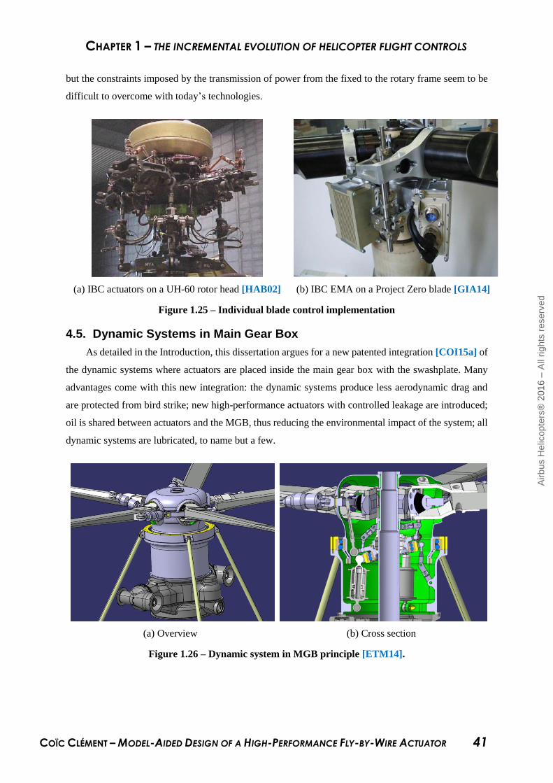
CHAPTER 1 – THE INCREMENTAL EVOLUTION OF HELICOPTER FLIGHT CONTROLS
COÏC CLÉMENT – MODEL-AIDED DESIGN OF A HIGH-PERFORMANCE FLY-BY-WIRE ACTUATOR 41
but the constraints imposed by the transmission of power from the fixed to the rotary frame seem to be
difficult to overcome with today’s technologies.
(a) IBC actuators on a UH-60 rotor head [HAB02] (b) IBC EMA on a Project Zero blade [GIA14]
Figure 1.25 – Individual blade control implementation
4.5. Dynamic Systems in Main Gear Box
As detailed in the Introduction, this dissertation argues for a new patented integration [COI15a] of
the dynamic systems where actuators are placed inside the main gear box with the swashplate. Many
advantages come with this new integration: the dynamic systems produce less aerodynamic drag and
are protected from bird strike; new high-performance actuators with controlled leakage are introduced;
oil is shared between actuators and the MGB, thus reducing the environmental impact of the system; all
dynamic systems are lubricated, to name but a few.
(a) Overview (b) Cross section
Figure 1.26 – Dynamic system in MGB principle [ETM14].
Airb
us H
elic
opte
rs®
2016 –
All
rights
reserv
ed

CHAPTER 1 – THE INCREMENTAL EVOLUTION OF HELICOPTER FLIGHT CONTROLS
COÏC CLÉMENT – MODEL-AIDED DESIGN OF A HIGH-PERFORMANCE FLY-BY-WIRE ACTUATOR 42
5. CONCLUSION
Helicopter flight controls have evolved incrementally from conventional designs, by progressively
adding new functions and components. In contrast, the FbW technology induced a re-engineering of the
flight control system architecture, as it required the current components to be replaced instead of simply
being upgraded. However, both technologies meet the same main functions with different
implementations that impact the level of safety associated to the fulfilment of each function.
Based on this observation, it has been decided to organize the presentation of the evolution of the
flight control system in this dissertation by the function each subsystem is aimed to fulfil. A generic
architecture and wording has been preferred for detailing the different technologies used for FbW
actuators. The recommendation to use DDV for primary flight controls has been addressed and the
opportunity to use EHSV for non-critical functions has been pointed out.
The next technological steps impacting the flight control system should be to keep increasing safety
and reduce helicopter vibration for passengers’ comfort. This should be made possible thanks to new
architectures of the Actuation System such as the integration of dynamic systems inside the main gear
box.
Airb
us H
elic
opte
rs®
2016 –
All
rights
reserv
ed

CHAPTER 1 – THE INCREMENTAL EVOLUTION OF HELICOPTER FLIGHT CONTROLS
COÏC CLÉMENT – MODEL-AIDED DESIGN OF A HIGH-PERFORMANCE FLY-BY-WIRE ACTUATOR 43
BIBLIOGRAPHY
[ATT08] ATTAR, B., Modélisation Réaliste en Conditions Extrêmes des Servovalves
Électrohydrauliques Utilisées pour le Guidage et la Navigation Aéronautique et
Spatiale. Toulouse, France, 2008. (in French)
[BOC04] BOCZAR, B. & HULL, B.J., S-92 Fly-by-Wire Advanced Flight Control System. AHS
60th Annual Forum, Baltimore, 2004.
[COI14] COÏC, C., ALLIETTA, J.-M., HENG, P. & BIHEL J.-R., Q670A0901E01 - Requirement
Specification for Main Rotor Actuator. Airbus Helicopters, Marignane, France, 2014.
(internal publication)
[COI15a] COÏC, C., BIHEL, J.-R., MARGER, T. & COUDERC, C., Patent US2015298796 (A1) -
Aircraft Hydraulic System Comprising at least one Servo-Control, and an associated
Rotor and Aircraft. Airbus Helicotpers, France, 2015.
[COI15b] COÏC, C. & HENG, P., Rapport de Synthèse, Choix de Technologie Actionneurs.
Marignane, France, 2015. (internal publication in French)
[COI16a] COÏC, C. & MARÉ, J.-C., Modeling and Pre-Sizing Process for Hydrostatic Thrust
Bearing with Special Consideration to Performance Robustness within a Wide
Temperature Range, International Conference on Hydraulics and Pneumatics, Praha,
Czech Republic, 2016.
[COI16b] COÏC, C., FU, J. & MARÉ, J.-C., Bond Graphs Aided development of Mechanical Power
Transmission for Aerospace Electromechanical Actuators, International Conference on
Bond Graph Modelling, Montréal, Canada, 2016.
[DON00] DONES, F., DRYFOOS, J.B., MCCORVEY, D.L. & HINDSON, W.S., An Advanced Fly-by-
Wire Flight Control System Designed for Airborne Research – Concept to Reality. AHS
56th Annual Forum, Virginia, 2000.
[EAS07] EUROPEAN AVIATION SAFETY AGENCY, Certification Specifications for Large
Rotorcraft, CS-29. Europe, 2007.
[EST15] ESTIVAL, P., Concept Innovant d’Actionneur Électromécanique pour la Commande de
Vol d’Hélicoptère de Nouvelle Génération. Paris, France, 2015. (in French)
[ETM14] ETM, Flight Controls Inside the Rotor Mast. Airbus Helicopters, France, 2015.
(internal publication)
[EUR04] EUROCOPTER, AS 332/532 “Super Puma”, Instruction Manual. Marignane, France,
2004
[FAA08] FEDERAL AVIATION ADMINISTRATION, Pilot’s Handbook of Aeronautical Knowledge.
U.S. Department of Transportation, 2008.
[FAA12] FEDERAL AVIATION ADMINISTRATION, Helicopter Flying Handbook. U.S. Department
of Transportation, 2012.
[FAA65] FEDERAL AVIATION ADMINISTRATION, Federal Aviation Regulations, Part 29,
Airworthiness Standards: Transport Category Rotorcraft. U.S. Department of
Transportation, 1965.
[FAI83] FAISANDIER, J., Mécanismes hydrauliques. Dunod, Paris, 1983. (in French)
Airb
us H
elic
opte
rs®
2016 –
All
rights
reserv
ed

CHAPTER 1 – THE INCREMENTAL EVOLUTION OF HELICOPTER FLIGHT CONTROLS
COÏC CLÉMENT – MODEL-AIDED DESIGN OF A HIGH-PERFORMANCE FLY-BY-WIRE ACTUATOR 44
[FOR88] FORMICA, B., KÖNIG, H., BENDER, K. & MANSFELD, G., A Digital Optical Tail Rotor
Control System. 14th European Rotorcraft Forum, Milano, 1988.
[FUE07] FUERST, D., Development, Prototype Production and Testing of an Electromechanical
Actuator for a Swashplateless Primary and Individual Helicopter Blade Control System.
Aircraft System Technologies, Hamburg, 2007.
[GIA14] GIANFRANCESCHI, M., JACAZIO, G. & WANG, J., High Bandwidth Electromechanical
Actuator for Swashplateless Blade Control System. International Conference on Recent
Advances in Actuation Systems and Components, R3ASC14, Toulouse, France, 2014.
[GLA26] GLAUERT, H., The Elements of Airfoil and Airscrew Theory. Cambridge University
Press, London, 1926.
[GRO13] GROHMANN, B., CHADUC, C. & TEMPIER C., Patent US2013168501 (A1) – Primary
Flight Controls, EUROCOPTER, 2013.
[GUI72] GUILLON, M., L’Asservissement Hydraulique et Élecrohydraulique, Tome 1, Théorie et
technique, Dunod, Paris, 1972. (in French)
[GUI92] GUILLON, M., Commande et asservissement hydrauliques et électrohydrauliques.
Lavoisier, Paris, 1992. (in French)
[HAB02] HABER, A., JACKLIN, S.A. & DESIMONE, G., Development, Manufacturing, and
Component Testing of an Individual Blade Control System for a UH-60 Helicopter
Rotor. AHS Aerodynamics, Acoustics, and Test and Evaluation Technical Specialists
Meeting, San Francisco, 2002.
[HIR04] HIRSCHEL, E.H., Aeronautical Research in Germany, from Lilienthal until Today.
Springer, 2004.
[JAA99] JOINT AVIATION AUTHORITIES, Joint Aviation Requirements, JAR-29, Large
Rotorcraft. Westward Digital Limited, United Kingdom 1926.
[KAS14] KASZYCKI, M. & PTACIN, R.R., Boeing 787-8 Design, Certification, and
Manufacturing Systems Review. Boeing & FAA, 2014.
[KIM14] KIM, S., The Bell 525 Relentless, The World’s First “Next Generation” Fly-by-Wire
Commercial Helicopter. AHS 70th Annual Forum, Montréal, Canada, 2014.
[MAR16] MARÉ, J.-C., Aerospace Actuators 1 : Needs, Reliability and Hydraulic Power
Solutions. Wiley-ISTE, 2016.
[MARG11] MARGER, T., Valve Design of Hydro-Mechanical Servoactuator under Cost and
Mixability Criteria. Arts et Métiers ParisTech, 2011.
[MAS78] MASKREY, R.H. & THAYER, W.J., A Brief History of Electrohydraulic
Servomechanisms. ASME Journal of Dynamic Systems Measurement and Control,
1978.
[MIL93] MILLER, F.G., Direct Drive Control Valves and their Applications. Proceedings of the
Institution of Mechanical Engineers: Aerospace Hydraulics & Systems, London, 1993.
[MOO87] MOOG, Type 30 Flow Control Servovalves. U.S.A., 1987.
[OSD88] OSDER, S.S., Digital Fly-by-Wire System for Advanced AH-64 Helicopters. AIAA/IEEE
8th Digital Avionics Systems Conference, San Jose, 1988.
Airb
us H
elic
opte
rs®
2016 –
All
rights
reserv
ed

CHAPTER 1 – THE INCREMENTAL EVOLUTION OF HELICOPTER FLIGHT CONTROLS
COÏC CLÉMENT – MODEL-AIDED DESIGN OF A HIGH-PERFORMANCE FLY-BY-WIRE ACTUATOR 45
[SAE96] SOCIETY OF AUTOMOTIVE ENGINEERS, ARP4761, Guidelines and Methods for
Conducting the Safety Assessment Process on Civil Airborne Systems and Equipment.
U.S.A., 1996.
[SAE00] SOCIETY OF AUTOMOTIVE ENGINEERS, AIR 1362 – Aerospace Hydraulic Fluids
Physical Properties. USA, 2000.
[SED89] SEDBON, G., Aérospatiale flies faster Dauphin. Flight International, 1989.
[SEE12] SEEMANN, S. & SCHLEGEL, C., Modeling and Simulation of a Fault-Tolerant
Electromechanical Actuation System for Helicopter Swashplates in Modelica.
International Conference on Recent Advances in Actuation Systems and Components,
R3ASC12, Toulouse, France, 2012.
[SNC55] SOCIETE NATIONALE DES CONSTRUCTIONS AERONAUTIQUES DU SUD-EST, SE.3130,
Manuel d’instruction. Marignane, France, 1955. (in French)
[SUD59] SUD-AVIATION, SA.316, Manuel d’instruction. Marignane, France, 1959. (in French)
[STI04] STILES, L.R., FREISNER, A.L., LANDIS, K.H. & KOTHMANN, B.D., “Impossible to
Resist”, The Development of Rotorcraft Fly-by-Wire Technology. AHS 60th Annual
Forum, Baltimore, 2004.
[VID97] VIDAL, P.A., NH 90 Helicopter Fly-by-Wire Flight Control System. Eurocopter, AHS
53th Annual Forum, Virginia, 2000.
[WRI99] WRIGHT, P., Helicopter Electro-mechanical Actuation Technology. IEE Colloquium on
Electrical Machines and Systems for the More Electric Aircraft, 1999.
Websites:
[webSITEC] www.sitec-aerospace.com/products/hydraulics.html,
accessed on 22/07/2016.
Airb
us H
elic
opte
rs®
2016 –
All
rights
reserv
ed
COÏC CLÉMENT – MODEL-AIDED DESIGN OF A HIGH-PERFORMANCE FLY-BY-WIRE ACTUATOR 46
CHAPITRE 2
MODELISATION ET SIMULATION DU SYSTEME D’ACTIONNEMENT
Ce chapitre introduit progressivement le besoin relatif à la modélisation de systèmes complexes
ainsi que des notions sur les Bond-graphs afin de modéliser chaque composant relatif au système
d’actionnement conformément `ce formalisme. Finalement, l’importance de la modélisation du système
dans sa globalité est accentuée par quelques scénarios simulés cet effet.
Il convient de rappeler en prélude de ce chapitre un certain nombre de termes relatifs à la
modélisation et simulation ainsi que quelques bonnes pratiques (non-exhaustives). La plupart de ces
termes sont présentés et développés dans le livre de François E. Cellier [CEL91] et il conviendra de se
référer à ce livre ou à la version anglaise de ce mémoire pour plus de détails.
Un modèle est une représentation d’un système, presque toujours simplifiée, réalisée dans le but
d’obtenir des informations sur ce dernier. En disant cela, il est sous-entendu que l’utilisateur du modèle
réalisera des essais sur celui-ci. Il est donc nécessaire de toujours associé à un modèle son domaine de
validité.
Un modèle n’est pas exclusivement un ensemble d’équations intégrées dans un logiciel
informatique. Un prototype physique d’un système pourra être appelé modèle même si cette appellation
est peu employée. À l’inverse, un modèle informatique extrêmement détaillé se verra parfois appelé
prototype virtuel afin de mettre l’accent sur sa représentativité.
La modélisation et la simulation d’un système lors de son cycle de vie sont aujourd’hui
omniprésentes. La Figure 2.1 présente la place que prennent les modèles lors d’un développement de
produit. Les modèles peuvent être utilisés dès la phase de spécification des exigences afin de s’assurer
de leur cohérence et compatibilité, lors de la sélection de l’architecture, de la solution technologique, du
dimensionnement ainsi que pour les essais unitaires et d’intégration système. Cette figure ne présente
pas l’utilité de ces mêmes modèles lorsque le produit est en cours d’utilisation afin de recréer des
phénomènes ou comportements observés, à moindre coût et de manière plus sûre. Aussi, nous pourrions
citer l’utilisation de modèles complémentaire pour l’optimisation des flux de production de ce système :
que ce soit pour la chaîne d’approvisionnement ou d’assemblage.
La version anglaise de ce chapitre détaille chacun de ces termes et essaye de les illustrer avec des
exemples relatifs à l’hydraulique. Un ensemble des sources d’erreurs possibles liées à la modélisation
et simulation y est aussi présentée.
Airb
us H
elic
opte
rs®
2016 –
All
rights
reserv
ed
CHAPITRE 2 – MODELISATION ET SIMULATION DU SYSTEME D’ACTIONNEMENT
COÏC CLÉMENT – MODEL-AIDED DESIGN OF A HIGH-PERFORMANCE FLY-BY-WIRE ACTUATOR 47
Le développement d’un modèle doit être mené de la même manière que le développement de tout
système. Pour cela, nous avons établi une liste de besoins relatifs au bon fonctionnement et au bon usage
des modèles. Cette liste est volontairement scindée en deux grandes familles : les besoins « génériques »
intrinsèques à l’ingénierie systèmes basée sur les modèles et les besoins « spécifiques » à l’industrie.
La suite de ce chapitre détaille les solutions choisies pour la modélisation sur la base de ces besoins.
Les Bond-graphs sont particulièrement bien adaptés aux critères génériques de par : leur généricité
multi-domaine, la représentation de phénomènes physiques facilement incrémentables, la formalisation
de l’attribution de causalité si souhaité, etc.
Sur la base du formalisme Bond-graphs, la topologie des modèles est présentée de manière
générique en insistant sur la lisibilité de ceux-ci. Pour ce faire, l’accent est porté sur la réticulation des
modèles, la différentiation des domaines physiques par des couleurs et la mise en avant des flux de
puissance principaux par rapport aux parasites. La Figure 2.4 contient l’ensemble de ces conventions
retenues.
Les recherches dans le cadre de cette thèse ont aussi conduit à la standardisation des modèles Bond-
graphs représentant le domaine mécanique. Cette standardisation a donné lieu à un article à la
« Conférence Internationale sur la Modélisation Bond-graphs » (International Conference on Bond-
Graphs Modeling) à Montréal en 2016 [COI16b]. Cette standardisation s’organise en deux sous-
systèmes majeures : les corps (Figure 2.5) et les interfaces mécaniques (Figure 2.6), tous deux modélisés
en translation et rotation. Les corps portent les éléments inertiels et s’interfacent avec les forces
extérieures ainsi que les interfaces standardisées. Les interfaces standardisées permettent les
mouvements relatifs entre corps et décomposent les efforts transmis en efforts normaux et tangentiels.
L’interface standardisée se veut générique et donc certains éléments peuvent être supprimés si les effets
modélisés ne sont pas souhaités. La généricité de cette standardisation est illustrée par la Figure 2.7,
laquelle représente plusieurs liaisons mécaniques types en Bond-graphs s’inscrivant parfaitement dans
le patron de l’interface standard.
L’application de l’ensemble des principes évoquées est portée sur la modélisation de système
d’actionnement dans la troisième partie de ce chapitre (§2.3). Le modèle de fluide est détaillé, présentant
les variables d’intérêt en fonction des phénomènes physiques modélisés, présents dans le formalisme
Bond-graph. Ensuite, les composants et leurs modèles sont présentés un par un, en essayant de présenter
l’état de l’art et justifiant les choix permettant de retenir une modélisation par composant.
Finalement, la quatrième partie de ce chapitre (§2.4) met en avant l’intérêt de la modélisation du
système d’actionnement en présentant les variations de performance du système face à différents
Airb
us H
elic
opte
rs®
2016 –
All
rights
reserv
ed

CHAPITRE 2 – MODELISATION ET SIMULATION DU SYSTEME D’ACTIONNEMENT
COÏC CLÉMENT – MODEL-AIDED DESIGN OF A HIGH-PERFORMANCE FLY-BY-WIRE ACTUATOR 48
scénarios des phénomènes relatifs aux charges antagonistes des actionneurs, la température de l’huile
ou encore les possibles couplages entre plusieurs actionneurs dans un même circuit.
Le modèle d’actionnement complet a été grandement utilisé en entreprise pour le pré-
dimensionnement du système d’actionnement d’un nouvel hélicoptère [COI16c], ainsi que pour la
modélisation sur simulateur de vol du système d’actionnement d’un hélicoptère existant.
Airb
us H
elic
opte
rs®
2016 –
All
rights
reserv
ed
COÏC CLÉMENT – MODEL-AIDED DESIGN OF A HIGH-PERFORMANCE FLY-BY-WIRE ACTUATOR 49
CHAPTER 2:
ACTUATION SYSTEM MODELLING & SIMULATION
1. INTRODUCTION
In order to homogenize the wording, it has been decided to introduce the specific terminology for
modelling and simulation in this section. Some terms have been defined in Continuous System Modeling
by François E. Cellier [CEL91]. However, it makes sense to select short extracts from this book,
complete them with new definitions and illustrate them with Actuation System examples to give the
reader a better understanding.
Once the principal terms have been introduced, the role of modelling and simulation in a new
development is presented. In contrast and to finish this introduction, it seems worthy to discuss the main
errors that modelling and simulation can bring with it.
1.1. Modelling and Simulation Terminology
Marvin Minsky gives a definition of a model that includes, specific terms needed for modelling
and simulation.
"A model (M) for a system (S) and an experiment (E) is anything to which E can be applied in order
to answer questions about S." [MIN65]
This definition of a model requires a clarification of the terms system and experiment.
1.1.1. System
The term system has already been used in this PhD dissertation as it is understood that a system is
a set of elements. But even though the term is understandable, most people using it only consider a
partial sense of it. The International Council on Systems Engineering (INCOSE) has the legitimacy to
provide its own definition of a system:
“A system is a construct or collection of different elements that together produce results not
obtainable by the elements alone. (…) The value added by the system as a whole, beyond that
contributed independently by the parts, is primarily created by the relationship among the parts;
that is, how they are interconnected.” [REC00]
Following this definition, a hydraulic cylinder includes, but is not limited to, a housing, a piston, a
rod, seals and oil. Oil-filled chambers are delimited by the piston and the housing. Sealing devices
Airb
us H
elic
opte
rs®
2016 –
All
rights
reserv
ed
CHAPTER 2 – ACTUATION SYSTEM MODELLING& SIMULATION
COÏC CLÉMENT – MODEL-AIDED DESIGN OF A HIGH-PERFORMANCE FLY-BY-WIRE ACTUATOR 50
prevent the oil to communicate between chambers via the piston-housing clearance. Relative movement
between piston and housing is possible. Therefore, the chambers’ volume is not necessarily constant.
Such relative movement creates an extension or retraction of the rod attached to the piston.
However, such definition does not explicitly include the possibility that a system could have
interfaces with other systems. By experience, a good system development consists in first defining its
boundaries and corresponding interfaces. In this example, the cylinder could exchange hydraulic power
through its ports and provide mechanical power at its mechanical interfaces (housing or rod). Therefore,
a more generic definition of a system, provided by Brian Gaines, is preferred.
“A system is characterized by the fact that we can say what belongs to it and what does not, and
by the fact that we can specify how it interacts with its environment.” [GAI79]
The notion of synergy, the interaction between parts or subsystems inside a system, is unfortunately
not explicit in Gaines definition. Without knowing the synergies inside a system, it is considered as a
black box. Its interest is limited as no internal variable is accessible. It is thus proposed to combine both
definitions and to redefine a system as follows: a system is characterized by the interactions with its
interfaces and by its synergies between its elements. Both synergies and interactions at interfaces can be
either functional or parasitic.
A last definition of a model is introduced by Bernard P. Zeigler and preferred by F.E. Cellier. It
could appear quite abstract but receives its meaning in the context of system study and testing.
“A system is a potential source of data.” [ZEI76]
This sentence fits perfectly with the following definition of an experiment.
1.1.2. Experiment
François E. Cellier provides a definition of the term experiment that seems clear and complete. The
term experiment is similar to the term test-case in the particular case of the Verification and Validation
(V&V) process.
"An experiment is the process of extracting data from a system by exerting it through its inputs."
[CEL91]
To the previously defined cylinder, a control valve is added in such a way that its spool position
modulates the hydraulic power transmitted to the cylinder chambers. This way, a hydraulic actuator is
obtained. A possible experiment could be to position the actuator on a test bench, connected to a
hydraulic power supply and without attaching the rod. By piloting a maximum opening of the valve, the
Airb
us H
elic
opte
rs®
2016 –
All
rights
reserv
ed
CHAPTER 2 – ACTUATION SYSTEM MODELLING& SIMULATION
COÏC CLÉMENT – MODEL-AIDED DESIGN OF A HIGH-PERFORMANCE FLY-BY-WIRE ACTUATOR 51
no-load maximum speed6 of the actuator (for a given pressure supply) would be extracted from this
experiment.
It appears relevant to emphasize that this definition does not make any particular reference to the
nature of the system or the nature of the experiment.
This definition also allows introducing the terms “controllable” and “observable”, which are
potential properties of a system. Referring to the system as a source of data implies that it is possible to
act on it (through its inputs) and to measure some variables (through its outputs). Selecting the variables
that are measured could impact the observability and controllability of variables [PRU70] or [GIL92].
1.1.3. Model
Marvin Minsky’s definition of a model quoted at the beginning of this chapter should now make
more sense. A model of a system is a representation of this system, created by a model architect, in order
to process experiments on it. This definition has strong consequences. It implies that the model is
sufficiently detailed and correctly implemented, based on the desired experiments so it can be used as a
substitution of the real system. This is indeed the correct way to model a system. The model user (who
may differ from the model architect) has to keep in mind that models are developed for a certain set of
experiments and adding an extra experiment may not be relevant if the model is not adapted. The set of
experiments is called the “experimental frame” by Bernard P. Zeigler [ZEI76]. The experimental frame
shall be accessible from the model to prevent misuse.
A model is a representation of a system and can be of different natures: hardware, software,
graphical scheme, etc. In order to be more explicit, it has been decided herein to introduce two subgroups
of models: virtual and physical models. The term virtual model is used for software models intended for
simulation, whereas hardware models are called physical models. In this PhD dissertation, these terms
are preferred as far as possible, as they provide additional information on the model type. Therefore, a
Bond-graph model of a hydraulic actuator can be called a virtual model, while a manufactured actuator
is a physical model.
1.1.4. Simulation
Granino Korn and John Wait define a simulation using the terms defined above.
"A simulation is an experiment performed on a model." [KOR78]
6 The no-load maximum speed is a characterising value of an actuator.
Airb
us H
elic
opte
rs®
2016 –
All
rights
reserv
ed
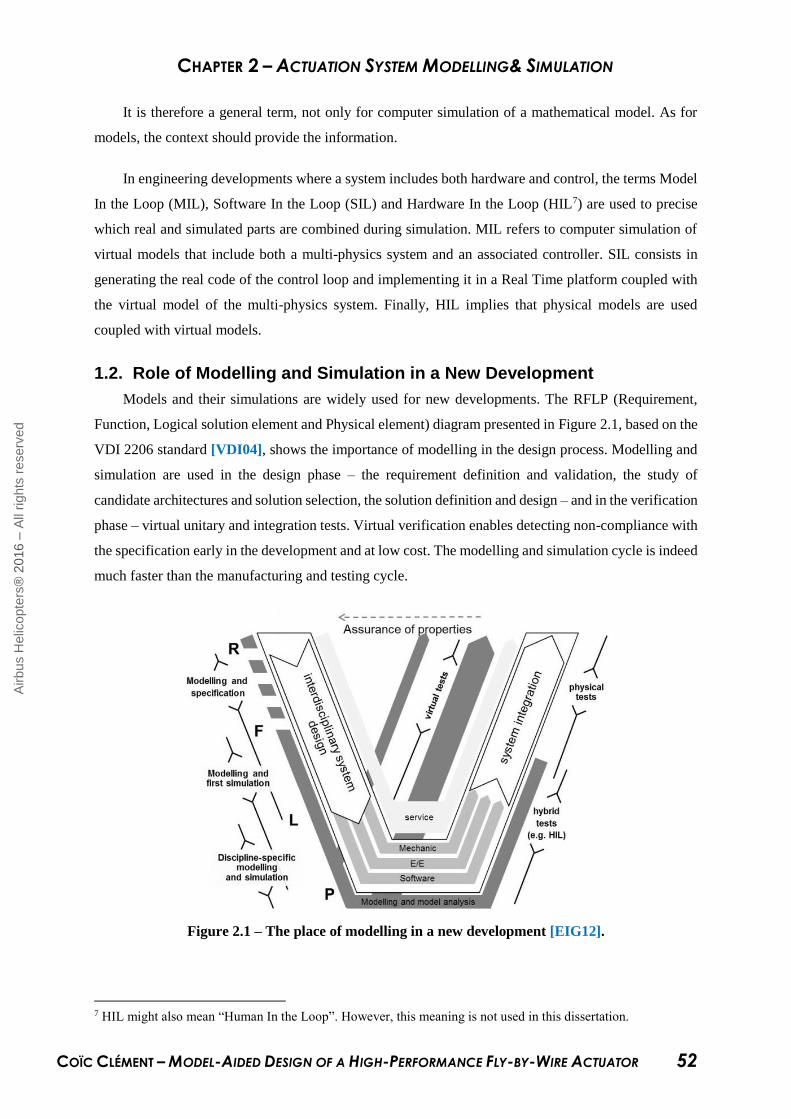
CHAPTER 2 – ACTUATION SYSTEM MODELLING& SIMULATION
COÏC CLÉMENT – MODEL-AIDED DESIGN OF A HIGH-PERFORMANCE FLY-BY-WIRE ACTUATOR 52
It is therefore a general term, not only for computer simulation of a mathematical model. As for
models, the context should provide the information.
In engineering developments where a system includes both hardware and control, the terms Model
In the Loop (MIL), Software In the Loop (SIL) and Hardware In the Loop (HIL7) are used to precise
which real and simulated parts are combined during simulation. MIL refers to computer simulation of
virtual models that include both a multi-physics system and an associated controller. SIL consists in
generating the real code of the control loop and implementing it in a Real Time platform coupled with
the virtual model of the multi-physics system. Finally, HIL implies that physical models are used
coupled with virtual models.
1.2. Role of Modelling and Simulation in a New Development
Models and their simulations are widely used for new developments. The RFLP (Requirement,
Function, Logical solution element and Physical element) diagram presented in Figure 2.1, based on the
VDI 2206 standard [VDI04], shows the importance of modelling in the design process. Modelling and
simulation are used in the design phase – the requirement definition and validation, the study of
candidate architectures and solution selection, the solution definition and design – and in the verification
phase – virtual unitary and integration tests. Virtual verification enables detecting non-compliance with
the specification early in the development and at low cost. The modelling and simulation cycle is indeed
much faster than the manufacturing and testing cycle.
Figure 2.1 – The place of modelling in a new development [EIG12].
7 HIL might also mean “Human In the Loop”. However, this meaning is not used in this dissertation.
Airb
us H
elic
opte
rs®
2016 –
All
rights
reserv
ed

CHAPTER 2 – ACTUATION SYSTEM MODELLING& SIMULATION
COÏC CLÉMENT – MODEL-AIDED DESIGN OF A HIGH-PERFORMANCE FLY-BY-WIRE ACTUATOR 53
In the descending part of the double V-cycle, the model becomes more and more detailed and,
simultaneously, the complexity usually increases. At the beginning of ascending part, the test
environment shall be ideal for characterizing the tested subsystem only, without coupling it with the real
environment. As the integration advances, the test environment realism increases to allow for a better
assessment of the entire system behaviour.
Therefore, the required models could be different for each phase of the RFLP process even if the
modelled system remains unchanged. This could be a cause of error in modelling and simulation
practices, but it is not the only one. It seems important to list the major errors that modelling and
simulation can bring with it if no particular care is taken.
1.3. Modelling and Simulation Errors
Virtual model simulation can support the development of new complex systems. It is a tool that
enables the prediction of the system’s behaviour. However, it must be kept in mind that the results
obtained always contain errors. These have to be defined and understood so that the model architect can
contain them and keep the simulation error at an acceptable level. Main errors come from:
Model representativeness. The virtual model of a system shall represent the relevant phenomena
of this system. However, it cannot reproduce the complete system. There are always more external
interactions and synergies than those that are modelled. For example, in fluid power modelling, it is
not usual to define the movement of each fluid particle but rather to define volumes with the
associated behaviour. Therefore, the molecular flow pattern on a porous filter is not modelled in
fluid power modelling. It is often a choice not to model certain phenomena. When a load of several
thousand newtons is applied to an actuator, maybe the gravity can be neglected. The model architect
shall ensure that the virtual model realized is representative of the experiments to be simulated on it
(each relevant phenomenon is present and correctly implemented). On his side, the model user shall
only run simulations for which the virtual model has been conceived.
Data correctness. It could appear obvious that the data used for the virtual model shall be entered
correctly. However, many errors at first simulations come from data provided with wrong units, sign
convention errors or erroneous initialization of state variables, etc.
Numerical robustness. Virtual models usually include state variables (if not, a virtual model may
not be needed but an algebraic model may be sufficient). A solver is used for the integration of the
state variables. The choice of the solver and the associated step size determines the numerical
stability and robustness of the simulation. For example, a stiff variable step solver would be
preferred for hydraulic systems due to high frequency modes (letting little space for numerical error),
whereas for Real Time simulation a fixed step solver is required (the step size shall be chosen with
caution).
Airb
us H
elic
opte
rs®
2016 –
All
rights
reserv
ed

CHAPTER 2 – ACTUATION SYSTEM MODELLING& SIMULATION
COÏC CLÉMENT – MODEL-AIDED DESIGN OF A HIGH-PERFORMANCE FLY-BY-WIRE ACTUATOR 54
Observation errors. It is common to plot simulation results. Caution should be exercised as plots
only present partial information (e.g. aliasing effect affecting sampled data). Also, solvers calculate
a finite number of points. Interpolations are performed between points in order to smooth the shape
of the plot. The model user has to ensure that these interpolations are legitimate.
Software constraints. Implementing a model in a software usually adds new constraints imposed
by software limitations. For example, generic models can require parameter values that are unknown
at this step of the development. Also, if the software is causal, it may require the addition of elements
for model interfacing even if the model architect would have neglected their effects, e.g. a
capacitance between two resistances or inertia between two compliances. These constraints tend to
decrease with software improvement: basic elements are usually available and combined with
hierarchical modelling; acausal languages such as Modelica are more and more used; tearing is a
solution for solving algebraic loops…
These sources of error are similar when dealing with physical models. The experimental frame shall
be defined. When testing a hydraulic actuator physical model, examples of each listed item could be:
Model representativeness: either if the physical model is complete and in final configuration for the
desired experimental frame, or the representativeness of its interfaces including the environment
(loads, vibration, temperature, etc.), the power supply (hydraulic pump, etc.), etc.
Data correctness: is the manufacturing of the actuator within its tolerances? Is the nominal pressure
of the hydraulic power source well set?
Numerical robustness: in case of electronic hardware or HIL testing, errors can arise from numerical
integrations.
Observation errors: for physical models, this could be for example sensor linearity, accuracy or error
and dynamics.
Software constraints: software is usually needed for HIL such as SIMULINK© for control design
and ControlDesk© for the Human Machine Interface (HMI).
In order to reduce possible representativeness errors, modelling needs are established. Model
architecting and development shall focus on meeting these needs.
2. MODEL ARCHITECTURE
Model architecture is probably the key for success in a virtual model development. It provides a
common structure to the models, leaving less room for the errors listed above.
This PhD dissertation first details the main modelling needs that have been identified by experience
and then the recommendations that can be derived from these needs. Bond-graphs are selected as a
modelling language and are thus introduced here. The main principles presented in this section are
Airb
us H
elic
opte
rs®
2016 –
All
rights
reserv
ed
CHAPTER 2 – ACTUATION SYSTEM MODELLING& SIMULATION
COÏC CLÉMENT – MODEL-AIDED DESIGN OF A HIGH-PERFORMANCE FLY-BY-WIRE ACTUATOR 55
already available in [COI16b]. In this paper, we detailed the development of a nut-screw for aerospace
EMA8 based on the engineering needs. In contrast, examples provided in this dissertation are more
oriented towards electro-hydraulic actuators. Also, modelling fluid power and electrical domains with
Bond-graphs is covered in this section.
2.1. Selected Modelling Needs
In order to focus on the engineering needs, engineering and industrial requirements are listed in
this section. It has been chosen to separate both kinds of requirements as the first kind involves good
practices that fit to the System Engineering process while the second kind could vary from one company
to another.
2.1.1. Engineering Requirements for Model Development
With reference to [MAR16], engineering requirements have been identified and are listed below.
In addition to this communication, it has been decided herein to provide the rationale associated with
each requirement so that the applicability can be discussed for each new development.
R1 Realism. The model architecture shall enable incremental modelling to progressively increase
realism regarding the key physical effects that impact performance. Models are a part of any step of a
complete development process, as detailed in section 1.2 and shown for RFLP in Figure 2.1. However,
the representativeness of the model can vary during the process depending on its aim.
R2 Genericity. As far as possible, the model shall be made up of a combination of generic sub-
models that can be re-used for other modelling purposes. This facilitates comprehension and
maintenance of the model (or library of models).
R3 Interfacing. The model shall have standard interfaces that are conserved throughout all
modelling levels. Defining standardized interfaces ensures the model’s connectivity and replaceability.
R4 Balancing. The model shall be balanced (mechanically, energetically, etc.). This reduces the
number of result misinterpretations by reproducing, for example, action and reaction forces (mechanical
balance). When thermal balance plays a key role in a system sizing, it is of particular interest to address
thermal power flows (energetic balance).
R5 Ageing and faults. The model shall enable ageing effects or faults to be simulated. This allows
representing the system’s behaviour over its entire lifespan as well as its response to faults. Transients
after a failure and degraded performance are usually sizing parameters for helicopter actuators.
8 Electro-Mechanical Actuators are introduced in Chapter 1 section 4.3, which is dedicated to PbW flight
controls.
Airb
us H
elic
opte
rs®
2016 –
All
rights
reserv
ed

CHAPTER 2 – ACTUATION SYSTEM MODELLING& SIMULATION
COÏC CLÉMENT – MODEL-AIDED DESIGN OF A HIGH-PERFORMANCE FLY-BY-WIRE ACTUATOR 56
R6 Causality. The model shall be developed to admit various causalities. For example, inverse
simulation is of great help for system sizing and integral causality on storage elements is preferred for
model simulation.
2.1.2. Industrial Requirements for Model Development
In addition to the engineering needs, industrial needs are defined. The industrial requirements listed
below are specific to this work and to the fact that the modelled system (the actuation system in our
case) is, indeed, a contributor to the global function performed by the Flight Control System. The flight
control system is modelled by another engineering team, using a simplified Actuation System model.
As both models are intended to interact, the simplified Actuation System model can be replaced by the
one developed within the scope of this PhD research.
R7 Workshare. The model shall correspond to the industrial workshare. The global interfaces of
the model shall thus be the real physical interfaces of the system as defined by the responsible Airbus
Helicopters department.
R8 Engineering. Model parameters shall be those which engineers are able to provide. They could
be specific to industrial experience or come from datasheet.
R9 Units. The data units provided to and extracted from the model parameters shall be the industrial
units.
R10 Export. The model shall have export capability to be interfaced with other models within the
interfacing standard of Airbus Helicopters.
R11 Documentation. The model shall include the information needed for its use and development,
including test cases.
R12 Capitalization. The model shall be a tool that facilitates further developments, easy to use by
simulation non-experts.
The last requirement needs to be detailed. It makes sense that a model is developed not only for the
model architect but for use by interested colleagues inside the company. They may not be familiar with
the overall system modelled and the complexity of the simulation environment shall be adapted
accordingly. However, these users shall be aware of simulation and the associated risks.
It is important to note that requirement R9 is not incompatible with using international system units
for calculation, which is a good basis to avoid errors in equations. Requirements R10 and R11 contribute
to requirement R12.
Airb
us H
elic
opte
rs®
2016 –
All
rights
reserv
ed
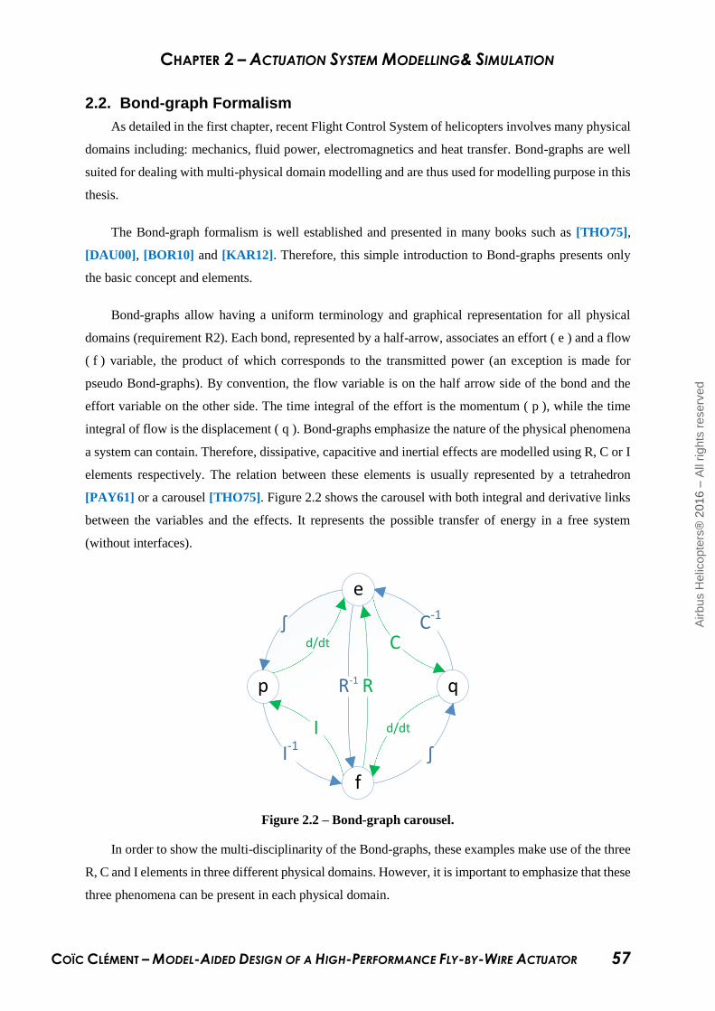
CHAPTER 2 – ACTUATION SYSTEM MODELLING& SIMULATION
COÏC CLÉMENT – MODEL-AIDED DESIGN OF A HIGH-PERFORMANCE FLY-BY-WIRE ACTUATOR 57
2.2. Bond-graph Formalism
As detailed in the first chapter, recent Flight Control System of helicopters involves many physical
domains including: mechanics, fluid power, electromagnetics and heat transfer. Bond-graphs are well
suited for dealing with multi-physical domain modelling and are thus used for modelling purpose in this
thesis.
The Bond-graph formalism is well established and presented in many books such as [THO75],
[DAU00], [BOR10] and [KAR12]. Therefore, this simple introduction to Bond-graphs presents only
the basic concept and elements.
Bond-graphs allow having a uniform terminology and graphical representation for all physical
domains (requirement R2). Each bond, represented by a half-arrow, associates an effort ( e ) and a flow
( f ) variable, the product of which corresponds to the transmitted power (an exception is made for
pseudo Bond-graphs). By convention, the flow variable is on the half arrow side of the bond and the
effort variable on the other side. The time integral of the effort is the momentum ( p ), while the time
integral of flow is the displacement ( q ). Bond-graphs emphasize the nature of the physical phenomena
a system can contain. Therefore, dissipative, capacitive and inertial effects are modelled using R, C or I
elements respectively. The relation between these elements is usually represented by a tetrahedron
[PAY61] or a carousel [THO75]. Figure 2.2 shows the carousel with both integral and derivative links
between the variables and the effects. It represents the possible transfer of energy in a free system
(without interfaces).
∫
C-1
I-1
∫ d/dt
p
I d/dt
RR-1
f
q
C
e
Figure 2.2 – Bond-graph carousel.
In order to show the multi-disciplinarity of the Bond-graphs, these examples make use of the three
R, C and I elements in three different physical domains. However, it is important to emphasize that these
three phenomena can be present in each physical domain.
Airb
us H
elic
opte
rs®
2016 –
All
rights
reserv
ed
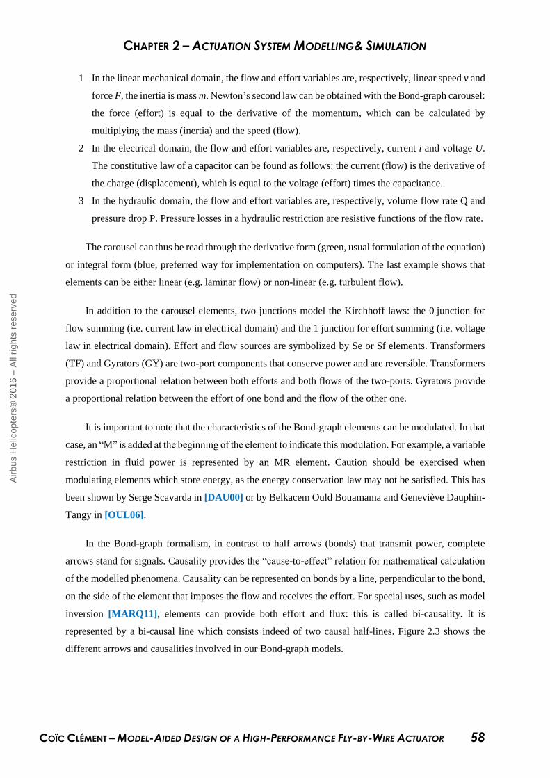
CHAPTER 2 – ACTUATION SYSTEM MODELLING& SIMULATION
COÏC CLÉMENT – MODEL-AIDED DESIGN OF A HIGH-PERFORMANCE FLY-BY-WIRE ACTUATOR 58
1 In the linear mechanical domain, the flow and effort variables are, respectively, linear speed v and
force F, the inertia is mass m. Newton’s second law can be obtained with the Bond-graph carousel:
the force (effort) is equal to the derivative of the momentum, which can be calculated by
multiplying the mass (inertia) and the speed (flow).
2 In the electrical domain, the flow and effort variables are, respectively, current i and voltage U.
The constitutive law of a capacitor can be found as follows: the current (flow) is the derivative of
the charge (displacement), which is equal to the voltage (effort) times the capacitance.
3 In the hydraulic domain, the flow and effort variables are, respectively, volume flow rate Q and
pressure drop P. Pressure losses in a hydraulic restriction are resistive functions of the flow rate.
The carousel can thus be read through the derivative form (green, usual formulation of the equation)
or integral form (blue, preferred way for implementation on computers). The last example shows that
elements can be either linear (e.g. laminar flow) or non-linear (e.g. turbulent flow).
In addition to the carousel elements, two junctions model the Kirchhoff laws: the 0 junction for
flow summing (i.e. current law in electrical domain) and the 1 junction for effort summing (i.e. voltage
law in electrical domain). Effort and flow sources are symbolized by Se or Sf elements. Transformers
(TF) and Gyrators (GY) are two-port components that conserve power and are reversible. Transformers
provide a proportional relation between both efforts and both flows of the two-ports. Gyrators provide
a proportional relation between the effort of one bond and the flow of the other one.
It is important to note that the characteristics of the Bond-graph elements can be modulated. In that
case, an “M” is added at the beginning of the element to indicate this modulation. For example, a variable
restriction in fluid power is represented by an MR element. Caution should be exercised when
modulating elements which store energy, as the energy conservation law may not be satisfied. This has
been shown by Serge Scavarda in [DAU00] or by Belkacem Ould Bouamama and Geneviève Dauphin-
Tangy in [OUL06].
In the Bond-graph formalism, in contrast to half arrows (bonds) that transmit power, complete
arrows stand for signals. Causality provides the “cause-to-effect” relation for mathematical calculation
of the modelled phenomena. Causality can be represented on bonds by a line, perpendicular to the bond,
on the side of the element that imposes the flow and receives the effort. For special uses, such as model
inversion [MARQ11], elements can provide both effort and flux: this is called bi-causality. It is
represented by a bi-causal line which consists indeed of two causal half-lines. Figure 2.3 shows the
different arrows and causalities involved in our Bond-graph models.
Airb
us H
elic
opte
rs®
2016 –
All
rights
reserv
ed
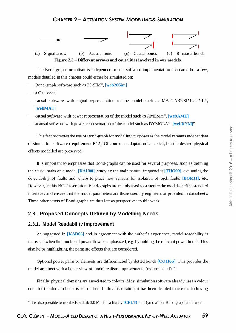
CHAPTER 2 – ACTUATION SYSTEM MODELLING& SIMULATION
COÏC CLÉMENT – MODEL-AIDED DESIGN OF A HIGH-PERFORMANCE FLY-BY-WIRE ACTUATOR 59
(a) – Signal arrow (b) – Acausal bond (c) – Causal bonds (d) – Bi-causal bonds
Figure 2.3 – Different arrows and causalities involved in our models.
The Bond-graph formalism is independent of the software implementation. To name but a few,
models detailed in this chapter could either be simulated on:
Bond-graph software such as 20-SIM©, [web20Sim]
a C++ code,
causal software with signal representation of the model such as MATLAB©/SIMULINK©,
[webMAT]
causal software with power representation of the model such as AMESim©, [webAME]
acausal software with power representation of the model such as DYMOLA©. [webDYM]9
This fact promotes the use of Bond-graph for modelling purposes as the model remains independent
of simulation software (requirement R12). Of course an adaptation is needed, but the desired physical
effects modelled are preserved.
It is important to emphasize that Bond-graphs can be used for several purposes, such as defining
the causal paths on a model [DAU00], studying the main natural frequencies [THO99], evaluating the
detectability of faults and where to place new sensors for isolation of such faults [BOR11], etc.
However, in this PhD dissertation, Bond-graphs are mainly used to structure the models, define standard
interfaces and ensure that the model parameters are those used by engineers or provided in datasheets.
These other assets of Bond-graphs are thus left as perspectives to this work.
2.3. Proposed Concepts Defined by Modelling Needs
2.3.1. Model Readability Improvement
As suggested in [KAR06] and in agreement with the author’s experience, model readability is
increased when the functional power flow is emphasized, e.g. by bolding the relevant power bonds. This
also helps highlighting the parasitic effects that are considered.
Optional power paths or elements are differentiated by dotted bonds [COI16b]. This provides the
model architect with a better view of model realism improvements (requirement R1).
Finally, physical domains are associated to colours. Most simulation software already uses a colour
code for the domain but it is not unified. In this dissertation, it has been decided to use the following
9 It is also possible to use the BondLib 3.0 Modelica library [CEL13] on Dymola© for Bond-graph simulation.
Airb
us H
elic
opte
rs®
2016 –
All
rights
reserv
ed
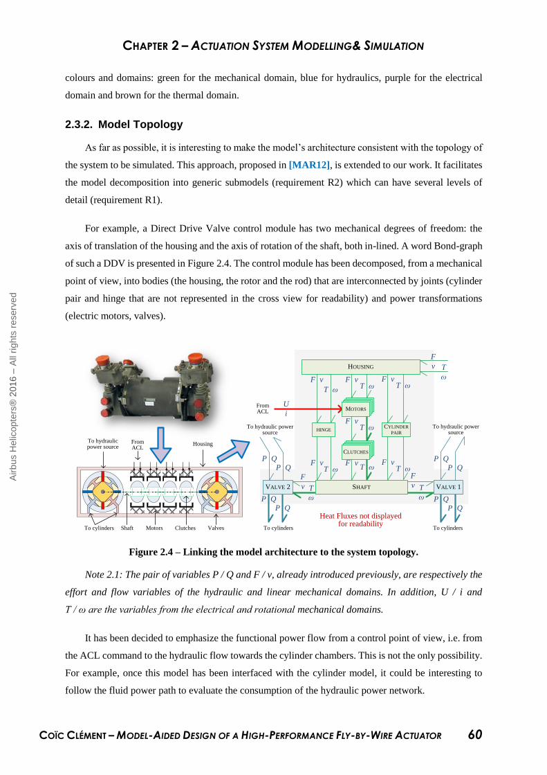
CHAPTER 2 – ACTUATION SYSTEM MODELLING& SIMULATION
COÏC CLÉMENT – MODEL-AIDED DESIGN OF A HIGH-PERFORMANCE FLY-BY-WIRE ACTUATOR 60
colours and domains: green for the mechanical domain, blue for hydraulics, purple for the electrical
domain and brown for the thermal domain.
2.3.2. Model Topology
As far as possible, it is interesting to make the model’s architecture consistent with the topology of
the system to be simulated. This approach, proposed in [MAR12], is extended to our work. It facilitates
the model decomposition into generic submodels (requirement R2) which can have several levels of
detail (requirement R1).
For example, a Direct Drive Valve control module has two mechanical degrees of freedom: the
axis of translation of the housing and the axis of rotation of the shaft, both in-lined. A word Bond-graph
of such a DDV is presented in Figure 2.4. The control module has been decomposed, from a mechanical
point of view, into bodies (the housing, the rotor and the rod) that are interconnected by joints (cylinder
pair and hinge that are not represented in the cross view for readability) and power transformations
(electric motors, valves).
MOTORS
To cylinders Motors Clutches ValvesShaft
To hydraulic power source
FromACL
Housing
MOTORSMOTORS
MOTORSMOTORSMOTORS
FromACL
To hydraulic power source
To hydraulic power source
To cylinders To cylinders
F v
T ω
F vT ω
F vT ω
F vT ω
F vT ω
F vT ω
F vT ω
F
v T
ω
F
v T
ω
F
v T
ω
VALVE 2 VALVE 1
HINGECYLINDER
PAIR
MOTORS
CLUTCHES
HOUSING
SHAFT
P QP Q
P QP Q
P QP Q
P QP Q
Heat Fluxes not displayed for readability
U
i
Figure 2.4 – Linking the model architecture to the system topology.
Note 2.1: The pair of variables P / Q and F / v, already introduced previously, are respectively the
effort and flow variables of the hydraulic and linear mechanical domains. In addition, U / i and
T / ω are the variables from the electrical and rotational mechanical domains.
It has been decided to emphasize the functional power flow from a control point of view, i.e. from
the ACL command to the hydraulic flow towards the cylinder chambers. This is not the only possibility.
For example, once this model has been interfaced with the cylinder model, it could be interesting to
follow the fluid power path to evaluate the consumption of the hydraulic power network.
Airb
us H
elic
opte
rs®
2016 –
All
rights
reserv
ed

CHAPTER 2 – ACTUATION SYSTEM MODELLING& SIMULATION
COÏC CLÉMENT – MODEL-AIDED DESIGN OF A HIGH-PERFORMANCE FLY-BY-WIRE ACTUATOR 61
2.3.3. Mechanical Balance
In the former example, both rotation and translation along the same axis are involved. Mechanical
balance (requirement R4) is thus reached by modelling each sub-model with mechanical quadriports
(linear and rotational power bonds for each body or interface). Indeed, to reach mechanical balance, the
number of ports should be an even number to reproduce action and reaction forces. In our application,
it is sufficient to consider one linear and one rotation axes, therefore four ports are needed. A particular
focus is laid on modelling mechanical elements in section 2.4, taking into account the quadriports
concept.
2.3.4. Energy Balance
As thermal balance plays a key role in the sizing and lifespan of a DDV’s motors, it is of particular
importance to enable the designers to address not only mechanical but also thermal power flows. For
this purpose, any energy loss (R element) is transformed into an RS field in order to output the heat
power P h that is generated by the loss effect (e.g. friction or even structural damping for mechanics).
As a very beneficial effect for embedded systems operating over a wide temperature range, using a
pseudo thermal bond enables the loss effect to be made sensitive to the temperature prevailing at the
thermal bond (e.g. influence of temperature on wire resistance and on friction). The objective of getting
energy-balanced models (requirement R4) has been applied to the following models unless it is explicitly
mentioned. However, for reasons of readability, thermal bonds are not represented except for direct
thermal coupling.
2.3.5. Fault Injection
During the development of safety-critical applications, it is important to assess the fault-to-failure
mechanism and the response to faults in case of progressive or sudden degradation. Simulation is
generally the only way to investigate the response to faults without danger (requirement R5). It is also
helpful for assessing fault signature and detectability during the design of health and usage monitoring
(HUM) features. In FbW systems, these features can be implemented at low cost thanks to the
availability of numerous sensor signals.
In the case of Figure 2.4, the model must be increased with fault triggering inputs to force either
progressive degradations (e.g. through real signals) or sudden faults (e.g. through Boolean inputs), as
suggested in [LIN14]. This is addressed in the following sections, dedicated to each domain modelling.
2.4. Proposed Standardization of the Mechanical Domain
When progressing from the preliminary to the detailed design phases, model complexity increases
versus realism. In this dissertation, standardized mechanical components are proposed to ensure
Airb
us H
elic
opte
rs®
2016 –
All
rights
reserv
ed
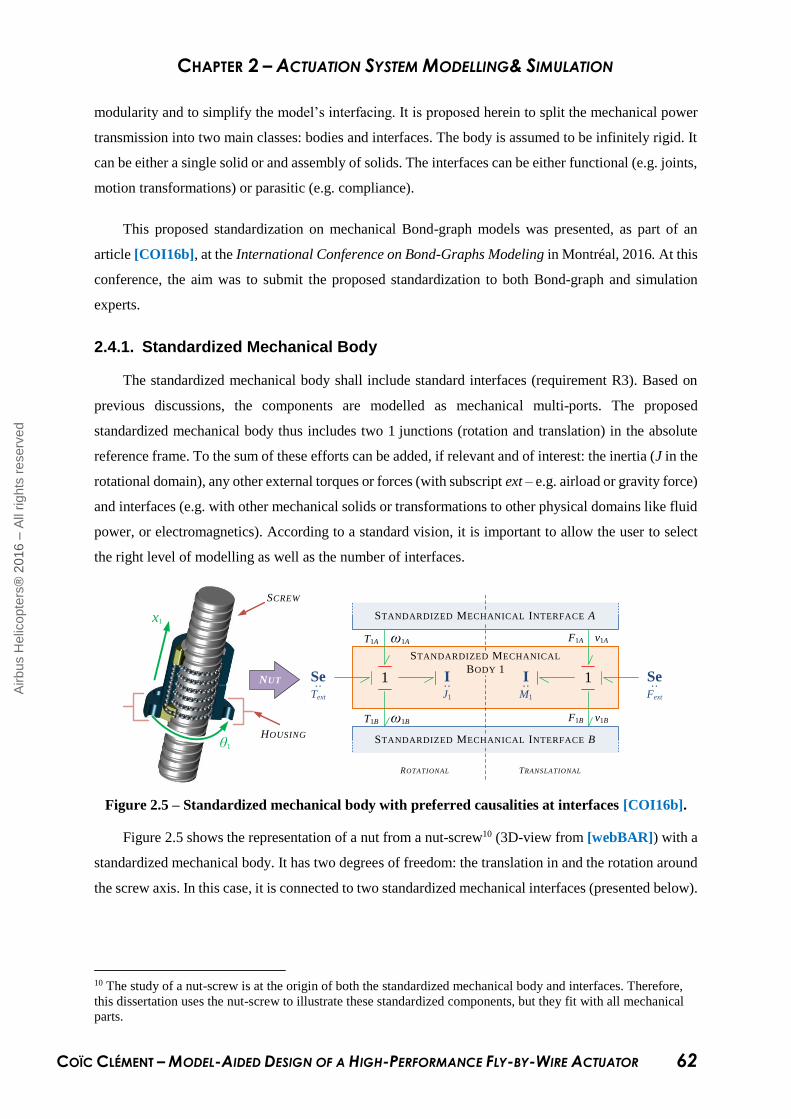
CHAPTER 2 – ACTUATION SYSTEM MODELLING& SIMULATION
COÏC CLÉMENT – MODEL-AIDED DESIGN OF A HIGH-PERFORMANCE FLY-BY-WIRE ACTUATOR 62
modularity and to simplify the model’s interfacing. It is proposed herein to split the mechanical power
transmission into two main classes: bodies and interfaces. The body is assumed to be infinitely rigid. It
can be either a single solid or and assembly of solids. The interfaces can be either functional (e.g. joints,
motion transformations) or parasitic (e.g. compliance).
This proposed standardization on mechanical Bond-graph models was presented, as part of an
article [COI16b], at the International Conference on Bond-Graphs Modeling in Montréal, 2016. At this
conference, the aim was to submit the proposed standardization to both Bond-graph and simulation
experts.
2.4.1. Standardized Mechanical Body
The standardized mechanical body shall include standard interfaces (requirement R3). Based on
previous discussions, the components are modelled as mechanical multi-ports. The proposed
standardized mechanical body thus includes two 1 junctions (rotation and translation) in the absolute
reference frame. To the sum of these efforts can be added, if relevant and of interest: the inertia (J in the
rotational domain), any other external torques or forces (with subscript ext – e.g. airload or gravity force)
and interfaces (e.g. with other mechanical solids or transformations to other physical domains like fluid
power, or electromagnetics). According to a standard vision, it is important to allow the user to select
the right level of modelling as well as the number of interfaces.
1
STANDARDIZED MECHANICAL INTERFACE B
Se··
Text
1I·· J1
I·· M1
ROTATIONAL TRANSLATIONAL
Se··
Fext
STANDARDIZED MECHANICAL INTERFACE A
F1A v1A T1A ω1A
F1B v1B T1B ω1B
STANDARDIZED MECHANICAL
BODY 1
θ1
x1
HOUSING
SCREW
NUT
Figure 2.5 – Standardized mechanical body with preferred causalities at interfaces [COI16b].
Figure 2.5 shows the representation of a nut from a nut-screw10 (3D-view from [webBAR]) with a
standardized mechanical body. It has two degrees of freedom: the translation in and the rotation around
the screw axis. In this case, it is connected to two standardized mechanical interfaces (presented below).
10 The study of a nut-screw is at the origin of both the standardized mechanical body and interfaces. Therefore,
this dissertation uses the nut-screw to illustrate these standardized components, but they fit with all mechanical
parts.
Airb
us H
elic
opte
rs®
2016 –
All
rights
reserv
ed

CHAPTER 2 – ACTUATION SYSTEM MODELLING& SIMULATION
COÏC CLÉMENT – MODEL-AIDED DESIGN OF A HIGH-PERFORMANCE FLY-BY-WIRE ACTUATOR 63
Interfaces A and B model its interfaces with the screw and with a schematic housing impeding
translational motion.
The choice of causality for simulation purpose is direct if the model architect decides to consider
component inertia. Otherwise, the model architect should define the causality in order to meet the
modularity requirement, as far as possible. This means that the causality on the interfaces should remain
unchanged. For example, in inverse simulation (requirement R6), a flow (speed) source can be added to
satisfy this need when no inertia is considered.
2.4.2. Standardized Mechanical Interface
The main idea behind the standard interface is to represent the power transmission between two
mechanical components as a combination of effort and flow losses in the plane tangent to contact (e.g.
between screw and nut threads). The proposed model makes causalities consistent with those of
standardized mechanical components. In that manner, it can be implemented in any causal simulation
environment.
In continuity with the standardized mechanical body, the interface in Figure 2.6 is illustrated in
analogy with a nut-screw interface. In this application, the plane of contact is the thread.
ST
AN
DA
RD
IZE
D M
EC
HA
NIC
AL
INT
ER
FA
CE A
STANDARDIZED MECHANICAL BODY 2
STANDARDIZED MECHANICAL BODY 1
0
T2A ω 2A
T1A ω1A
0
F2A v2A
F1A v1A
1 1
MTF 0
0
MRS
1 MRSC
Jamming
Wear
De
0
TO
TH
ER
MA
L
MO
DE
L
Temperature sensitivity
Stiffness Damping
Friction losses
NORMAL AXIS
TANGENTIAL AXIS
θ Ph
NUT-SCREW
I N TERFACE
rm
MTF
MTF MTF
Dilatation
Figure 2.6 – Standardized mechanical interface with the preferred causality [COI16b].
In the normal axis of the plane of contact, the flow losses are placed on a 0 junction which receives
flow variables from the mechanical solids through transformers and . In the particular case of nut-
screws, transformer ratios and equal respectively (rmcosβsinα) and 1/(cosβcosα), where α is the
helix angle, β the thread angle and rm the mean radius. Relative velocity is computed and transmitted to
Airb
us H
elic
opte
rs®
2016 –
All
rights
reserv
ed

CHAPTER 2 – ACTUATION SYSTEM MODELLING& SIMULATION
COÏC CLÉMENT – MODEL-AIDED DESIGN OF A HIGH-PERFORMANCE FLY-BY-WIRE ACTUATOR 64
the optional compliance (C field) and dissipative (MRS field) for effort calculation. In the C field,
preload or play can be considered and rupture can be triggered.
The effort losses, which are mainly due to sliding friction, are calculated in the plane of contact and
receive the sign for relative velocity between the two component surfaces. Therefore, frictional loss is
represented as an MRS field connected to a 0 junction. It is modulated by the effort component acting
perpendicularly on the contact point. This simply denotes that due to friction, the tangent force is directly
dependent on the normal force applied at contact. Effort losses are transmitted to the mechanical solids
through transformers and , which respectively equal (rmcosα) and (sinα) for a nut-screw interface.
Jamming can be easily triggered by increasing the amount of friction in the MRS element
implementation and friction can be made dependent on the transmitted force and temperature (in
addition to the dependency on velocity induced by the constitutive law of an R element).
Note 2.2: Modulated transformers are used in the standardized mechanical interface for
generalization purposes. In the particular case of nut-screws, the transformers have constant ratios.
However, in many applications the ratio varies, e.g. the swashplate angle of a variable displacement
pump.
Both flow and effort losses apply to relative motion. To keep it as general as possible, this model
structure includes four transformation elements for each projection in the normal and tangential
directions of the contact interface plane. However, if a transformation is not relevant, it can be withdrawn
or affected by a unity ratio. In the same modular approach, compliance and resistance elements are
placed in the normal axis that the modeller can remove if it is not relevant. In this drawing, the thermal
power bonds are represented in order to fulfil the thermal balance (requirement R4).
The modularity and genericity is the strength of the proposed standardized mechanical interface. It
covers any mechanical interface. This is highlighted by addressing the Bond-graph models of several
functional interfaces, as illustrated in Figure 2.7 for hinge pair, prism pair, cylinder pair, nut/screw and
dog-teeth.
Airb
us H
elic
opte
rs®
2016 –
All
rights
reserv
ed
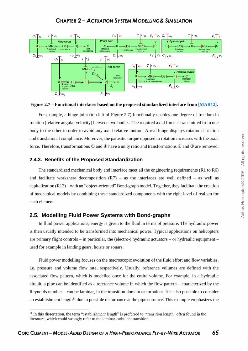
CHAPTER 2 – ACTUATION SYSTEM MODELLING& SIMULATION
COÏC CLÉMENT – MODEL-AIDED DESIGN OF A HIGH-PERFORMANCE FLY-BY-WIRE ACTUATOR 65
Figure 2.7 – Functional interfaces based on the proposed standardized interface from [MAR12].
For example, a hinge joint (top left of Figure 2.7) functionally enables one degree of freedom in
rotation (relative angular velocity) between two bodies. The required axial force is transmitted from one
body to the other in order to avoid any axial relative motion. A real hinge displays rotational friction
and translational compliance. Moreover, the parasitic torque opposed to rotation increases with the axial
force. Therefore, transformations and have a unity ratio and transformations and are removed.
2.4.3. Benefits of the Proposed Standardization
The standardized mechanical body and interface meet all the engineering requirements (R1 to R6)
and facilitate workshare decomposition (R7) – as the interfaces are well defined – as well as
capitalization (R12) – with an “object-oriented” Bond-graph model. Together, they facilitate the creation
of mechanical models by combining these standardized components with the right level of realism for
each element.
2.5. Modelling Fluid Power Systems with Bond-graphs
In fluid power applications, energy is given to the fluid in terms of pressure. The hydraulic power
is then usually intended to be transformed into mechanical power. Typical applications on helicopters
are primary flight controls – in particular, the (electro-) hydraulic actuators – or hydraulic equipment –
used for example in landing gears, hoists or sonars.
Fluid power modelling focuses on the macroscopic evolution of the fluid effort and flow variables,
i.e. pressure and volume flow rate, respectively. Usually, reference volumes are defined with the
associated flow pattern, which is modelled once for the entire volume. For example, in a hydraulic
circuit, a pipe can be identified as a reference volume in which the flow pattern – characterized by the
Reynolds number – can be laminar, in the transition domain or turbulent. It is also possible to consider
an establishment length11 due to possible disturbance at the pipe entrance. This example emphasizes the
11 In this dissertation, the term “establishment length” is preferred to “transition length” often found in the
literature, which could wrongly refer to the laminar-turbulent transition.
Airb
us H
elic
opte
rs®
2016 –
All
rights
reserv
ed

CHAPTER 2 – ACTUATION SYSTEM MODELLING& SIMULATION
COÏC CLÉMENT – MODEL-AIDED DESIGN OF A HIGH-PERFORMANCE FLY-BY-WIRE ACTUATOR 66
possibility to change flow patterns (or even have two of them at the same time) for a given volume, but
it is modelled only once for the entire volume. For a more detailed view of the flow pattern, it could be
interesting to model the evolution of each fluid particle, but then the simulation would have to be carried
out with another detailed CFD model.
2.5.1. Energetic Balance in Fluid Power Modelling
Energetic balance (R4) requires a thermo-hydraulic model of the internal energy of the fluid.
However, this is not addressed in this fluid model for two main reasons:
The complexity added by thermo-hydraulic modelling counters requirements R8 (engineering
parameters) and R9 (industrial units). Fluid power engineers usually are more comfortable with
“Bar” and L”/min” than with “Pa”, “kg/s” and “kJ”.
Precise modelling of the thermal properties of the fluid is useless without a detailed model of the
hydraulic system environment for thermal exchanges. Unfortunately, such an environment model is
highly dependent on each helicopter and is therefore not available at the beginning of a new
development. At Airbus Helicopters, the thermo-hydraulic model is developed at the end of the
rotorcraft development (after cold and hot flight test campaign) to investigate specific behaviours
under harsh conditions.
Therefore, the thermal effect is partially addressed in this dissertation. The fluid temperature – and
with it its intrinsic properties – can be imposed (by an input variable in the model) but is considered
constant all along the virtual model at a given simulation time. This hypothesis is made when dealing
with hydraulic power Bond-graphs (using pressure and flow rate as effort and flow variables).
Local dissipation is computed (RS element), which provides a good approximation of the resulting
created heat. It makes the model ready for interfacing with the environment model for a first estimation.
2.5.2. Volume Computation
In this dissertation, Bond-graph models are used to structure the virtual model. The lack of a Bond-
graph simulation environment at Airbus Helicopters forces the implementation with another simulation
software, usually causing the engineer to convert the Bond-graphs into equations. But the equations
obtained from Bond-graphs may slightly differ from one engineer to another.
Airb
us H
elic
opte
rs®
2016 –
All
rights
reserv
ed

CHAPTER 2 – ACTUATION SYSTEM MODELLING& SIMULATION
COÏC CLÉMENT – MODEL-AIDED DESIGN OF A HIGH-PERFORMANCE FLY-BY-WIRE ACTUATOR 67
C
e3 f3
0e1
f1
e2
f2
(a) – Causal Bond-graph (b) – Volume computation (c) – Continuity equation
Figure 2.8 – Bond-graph of a hydraulic capacitive effect and two possible implementations.
Note 2.3: In Figure 2.8, the C element is represented as a gain. It is a simplification to illustrate
this point. The result would have been the same considering C as a function of displacement q.
As an example, a capacitive effect is considered as pictured by the causal Bond-graph in Figure 2.8-
(a). In the hydraulic domain, this corresponds to the compression (or decompression) of a fluid in a
volume, thus converting flow rate into pressure (or vice-versa). Integral causalities are shown in order
to support the implementation in simulation software.
To continue with the hydraulic example, one engineer could apply strictly the rules of Bond-graphs
stating that:
3 1 2
3 3
1 3
2 3
1
f f f
e f dtC
e e
e e
Equation 2.1
It is possible to see that, in the second member of Equation 2.1, the computation of the generalized
displacement (volume for hydraulics) is performed first and is then affected by the inverse of the
capacitance (the stiffness). This is convenient as volumes are the state variable of fluid power systems.
It is even more convenient to make appear volumes V1 and V2, which is possible as the time integral of
the volume flow rate is a first order homogeneous function. Thus, it is possible to assess the filling of a
chamber with oil or, in other words, the quantity of air in the chamber. Unfortunately, negative values
of volume 3 lead to negative values of pressure in the 0 junction. It is then necessary to either stop the
simulation or impose a zero low limit to the pressure values. Also, if the compressibility is dependent
on the effort, as is usually the case in hydraulics, where the Bulk modulus is a function of the pressure,
an algebraic loop appears. The corresponding block diagram is shown in Figure 2.8-(b).
In fluid power, engineers usually apply the continuity equation to volumes [GUI92]. This equation
first divides volume flow rate Q3 by the capacitance, and then integrates the result with respect to the
time (Equation 2.2). The corresponding block diagram is shown in Figure 2.8-(c).
Airb
us H
elic
opte
rs®
2016 –
All
rights
reserv
ed
CHAPTER 2 – ACTUATION SYSTEM MODELLING& SIMULATION
COÏC CLÉMENT – MODEL-AIDED DESIGN OF A HIGH-PERFORMANCE FLY-BY-WIRE ACTUATOR 68
3 3
1e f dt
C Equation 2.2
In this case, it is not possible to perceive the volume values. However, this solution has the
advantage that the Bulk modulus (included in the capacitance) can be made dependent on the pressure
without creating an algebraic loop.
Note 2.4: It is important to note that the continuity equation is equivalent to the equation derived
from Bond-graphs only if the C element is constant with time and can thus be introduced in the time
integral. However, the continuity equation is usually applied to time variable volumes such as cylinder
chambers. On the contrary, in Bond-graphs, C elements modulated with signal inputs should not exist
[BEA88].
2.6. Electrical Systems with Bond-graphs
Electrical models are developed in analogy with hydraulic models. The temperature is made
accessible with an input variable but is considered constant in the entire electrical circuit. For example,
a resistance is the function of the temperature. Herein, it is modelled with an RS element, the
characteristic of which is temperature-dependent and from which the Joule losses are computed. But no
coupling is performed at this level, so the Joule losses do not affect the resistance temperature.
Bond-graph modelling of electrical systems has been studied in more detail at the Institut Clément
Ader laboratory. For example, Jian Fu [FU15] modelled EMAs and their power electronics with Bond-
graphs. This is why this subject is not studied more thoroughly in this dissertation.
3. ACTUATION SYSTEM VIRTUAL MODEL
In this section, the purpose of actuation system modelling is detailed with its interfaces. Then each
subsystem is modelled with Bond-graphs in a component-oriented manner.
3.1. Purpose of Actuation System modelling
In this PhD dissertation, an Actuation System covers hydraulic power generation and distribution,
and main and tail rotors actuators (Figure 2.9).
The Actuation System is a dominant contributor to the Flight Control System’s overall
performance. Actuation system design shall take into account severe environmental and hydraulic power
consumption constraints. If managed independently, these two levels of constraints – functional needs
(piloting) and environmental constraints (oil temperature, failures, etc.) – could lead to oversizing or
undersizing of the Actuation System design. Incorrect sizing generates undue costs and weight increases
(oversizing) or operational limitations (undersizing), which negatively impact helicopter final design or
performance.
Airb
us H
elic
opte
rs®
2016 –
All
rights
reserv
ed
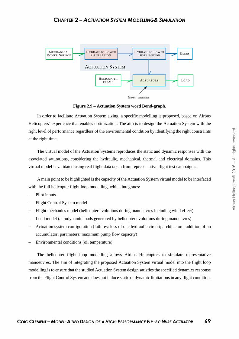
CHAPTER 2 – ACTUATION SYSTEM MODELLING& SIMULATION
COÏC CLÉMENT – MODEL-AIDED DESIGN OF A HIGH-PERFORMANCE FLY-BY-WIRE ACTUATOR 69
HYDRAULIC POWER D ISTRIBUTION
HYDRAULIC POWER GENERATION
MECHANICAL POWER SOURCE
ACTUATORS LOAD
USERS
ACTUATION SYSTEM
HELICOPTER
FRAME
INPUT ORDERS
Figure 2.9 – Actuation System word Bond-graph.
In order to facilitate Actuation System sizing, a specific modelling is proposed, based on Airbus
Helicopters’ experience that enables optimization. The aim is to design the Actuation System with the
right level of performance regardless of the environmental condition by identifying the right constraints
at the right time.
The virtual model of the Actuation Systems reproduces the static and dynamic responses with the
associated saturations, considering the hydraulic, mechanical, thermal and electrical domains. This
virtual model is validated using real flight data taken from representative flight test campaigns.
A main point to be highlighted is the capacity of the Actuation System virtual model to be interfaced
with the full helicopter flight loop modelling, which integrates:
Pilot inputs
Flight Control System model
Flight mechanics model (helicopter evolutions during manoeuvres including wind effect)
Load model (aerodynamic loads generated by helicopter evolutions during manoeuvres)
Actuation system configuration (failures: loss of one hydraulic circuit; architecture: addition of an
accumulator; parameters: maximum pump flow capacity)
Environmental conditions (oil temperature).
The helicopter flight loop modelling allows Airbus Helicopters to simulate representative
manoeuvres. The aim of integrating the proposed Actuation System virtual model into the flight loop
modelling is to ensure that the studied Actuation System design satisfies the specified dynamics response
from the Flight Control System and does not induce static or dynamic limitations in any flight condition.
Airb
us H
elic
opte
rs®
2016 –
All
rights
reserv
ed

CHAPTER 2 – ACTUATION SYSTEM MODELLING& SIMULATION
COÏC CLÉMENT – MODEL-AIDED DESIGN OF A HIGH-PERFORMANCE FLY-BY-WIRE ACTUATOR 70
3.2. Fluid Modelling
3.2.1. Needs of a Fluid Model
In this dissertation, the reference fluid used is the MIL-PRF-83282 [SAE00]. The performance
variations of the Actuation System with the pressure ( P ) and temperature ( T ) are mainly due to the
change of oil intrinsic properties. The fluid model shall thus provide the intrinsic properties needed by
the Bond-graph elements:
The I element requires the mass density: ρ in [kg/m3]. It represents the mass of fluid per unitary
volume. It is necessary to compute inertial forces involved in transients such as the “water hammer”
effect or line dynamics, to name but a few.
The R element requires:
o the absolute viscosity: µ in [Pa.s]. It characterizes the fluid resistance to flow. It is the
principal contributor to performance evolution with temperature: it creates high pressure
drops at low temperatures and increases the leakage at high temperatures.
o the mass density for several calculations such as the Reynolds number (through the link
between kinematic and absolute viscosity), or for pressure losses under turbulent flow.
The C element requires the Bulk modulus: β in [Pa]. It provides the relation between pressure and
volume variations. It is thus mandatory for modelling the oil compressibility. Four Bulk moduli can
be defined: adiabatic tangent or secant and isothermal tangent or secant. The SAE [SAE00] states
that system sizing in fluid power applications requires adiabatic Bulk moduli. Tangent is used for
small variations of pressure (e.g. pipe, actuator…) while secant is for large variations (e.g.
pumps…). In practice, a single Bulk modulus is measured by tests and used for all applications.
The evolution of these properties is thus presented regarding pressure and temperature, based on
[SAE00] for the fluid MIL-PRF-83282. Note that the operating temperature range defined in table 2 of
this information report for this fluid is [Tmin;Tmax]=[-40;+205]°C. This range is the basis for temperature
normalization in this dissertation (e.g. in Chapter 3 for the dimensionless design of fluid bearings).
According to Figure 2.10-(a), the density varies by less than 20 % of its maximum value over the
total range of the operating temperature. On its side, the kinematic viscosity is affected by a factor of
nearly 3000 from -40°C to +195°C, according to Figure 2.10-(b). With this comparison, it is already
possible to anticipate that the viscosity will play a major role in fluid power applications operating in a
wide temperature range. Change of density and viscosity with pressure should be modelled but should
have a limited impact on the simulation results, except for the transient effect in hydraulic capacitances.
Airb
us H
elic
opte
rs®
2016 –
All
rights
reserv
ed

CHAPTER 2 – ACTUATION SYSTEM MODELLING& SIMULATION
COÏC CLÉMENT – MODEL-AIDED DESIGN OF A HIGH-PERFORMANCE FLY-BY-WIRE ACTUATOR 71
(a) – Mass density characteristic (b) – Kinematic viscosity characteristic
(c) – Adiabatic tangent Bulk modulus (d) – Adiabatic secant Bulk modulus
Figure 2.10 – MIL-PRF-83282 properties,
oil sensitivity to temperature and pressure taken from [SAE00].
3.2.2. Mass Density
A first order Taylor expansion can be used to model a linear dependency of the fluid density on
temperature and pressure [ATT08]. These assumptions from -40°C to +205°C and from 0 Bar to
275.6 Bar, combined with a good identification of partial derivatives, lead to a maximum error of 2 %
compared to values extracted from Figure 2.10-(a). Subscript “0” corresponds to the reference point.
( , ) 0 0 0
T
( ) ( )T P
P
T T P PT P
Equation 2.3
It is relevant to emphasize the meaning of the partial derivatives involved in Equation 2.3:
0
1P
PT
is the coefficient of thermal expansion expressed in [°C-1]. It represents the
relation between the variation of density and temperature. Fortunately for our fluid model, it can be
considered constant regarding pressure and temperature for the operating range. It equals 8.2x10-
4°C-1 for MIL-PRF-83282 [SAE00].
Airb
us H
elic
opte
rs®
2016 –
All
rights
reserv
ed

CHAPTER 2 – ACTUATION SYSTEM MODELLING& SIMULATION
COÏC CLÉMENT – MODEL-AIDED DESIGN OF A HIGH-PERFORMANCE FLY-BY-WIRE ACTUATOR 72
, 0t i
T
P
is the tangent isothermal Bulk modulus.
These remarks have strong implications for the fluid model. Interrelations exist between the mass
density, the coefficient of thermal expansion and the Bulk modulus. In this dissertation, it has been
decided to model the mass density as a function of both αp and β (and T0 and P0). Therefore, in addition
to the three initial intrinsic properties required by the Bond-graph elements listed above, the coefficient
of thermal expansion is added.
3.2.3. Absolute Viscosity
Fluid viscosity is often approximated by an exponential decrease with the increase of temperature
[SAE00] [ATT08]. However, different fittings exist for temperature dependency, e.g. the one provided
by Faisandier [FAI83], which uses the Barus equation [BAR93] for the pressure dependency.
( , ) 0 0 0exp ln( )*( / ) ( )a
T P T T k P P Equation 2.4
where:
a is the fluid viscosity index [-]
k is a pressure-viscosity coefficient, which varies with temperature [Pa-1]
In this dissertation, tables are preferred to model the fluid properties. Indeed, most of the data are
taken from tables of the AIR 1362 [SAE00]. Trying to fit equations to these points is an additional
source of error which is not desirable.
3.2.4. Bulk Modulus
Figure 2.10-(c) and Figure 2.10-(d) show the adiabatic tangent and secant Bulk moduli. Their
values for a relative pressure of 0 MPa is quite similar. The adiabatic tangent Bulk modulus appears
more strongly influenced by pressure increase than the secant Bulk modulus. In practice, once the effect
of entrained air and the compression of mechanical parts are taken into account, it is possible to consider
a single equivalent Bulk modulus as a function of both the pressure and the temperature. In our
application, simulation results are sufficiently accurate with this approach. In practice, the equivalent
Bulk modulus also includes the elasticity of the fluid envelope (e.g. pipe, actuator housing…), as
detailed for example in [MER67] or [GUI92].
Several models exist to fit the Bulk modulus evolution with temperature and pressure, such as
[BOE95], [EGG80], [HOF81], [JIN94] or [LEE77]. However, as for the absolute viscosity, tables
have been preferred to model a single Bulk modulus.
Airb
us H
elic
opte
rs®
2016 –
All
rights
reserv
ed

CHAPTER 2 – ACTUATION SYSTEM MODELLING& SIMULATION
COÏC CLÉMENT – MODEL-AIDED DESIGN OF A HIGH-PERFORMANCE FLY-BY-WIRE ACTUATOR 73
3.3. Hydraulic System Virtual Model
The hydraulic system virtual model includes the hydraulic reservoirs, power generation and
distribution.
As presented in Chapter 1, the flight control system – and thus the Actuation System – ensures a
safety-critical function. Therefore, it is necessary to design the hydraulic system including redundancies
to meet the flight control system reliability requirement.
ACTUATION SYSTEM
HYDRAULIC RESERVOIRS
HYDRAULIC POWER
GENERATION
HYDRAULIC POWER
DISTRIBUTION
ACTUATORS
AUXILIARY CONSUMERS
Figure 2.11 – H225 Hydraulic System with the main users identified from [EUR04].
In our helicopter, usually one “clean” circuit only generates and distributes hydraulic power to the
lower cylinders of the main and tail rotor actuators; another hydraulic circuit is connected to the upper
actuator cylinders and to the other auxiliary consumers (landing gear, wheel and rotor brakes, automatic
pilot and hoist).
Figure 2.11 shows a representation of the two hydraulic systems of an AS332 with the main
consumers identified. The Actuation System and its main subsystem are highlighted.
In this PhD dissertation, an effort is made to accurately model the Hydraulic System in terms of
pressure losses, fluid dynamics, generated heat, etc. At this level, actuators are considered as power
consumers. They are modelled in section 3.3. Auxiliary consumers are also considered as power
consumers but are not modelled in more detail as they are under the responsibility of another Airbus
Helicopters department (requirement R7). However, model interfaces are created and enable further
connection with auxiliary consumer models.
Airb
us H
elic
opte
rs®
2016 –
All
rights
reserv
ed

CHAPTER 2 – ACTUATION SYSTEM MODELLING& SIMULATION
COÏC CLÉMENT – MODEL-AIDED DESIGN OF A HIGH-PERFORMANCE FLY-BY-WIRE ACTUATOR 74
3.3.1. Hydraulic Reservoir Virtual Model
In most Airbus Helicopters simulations, the hydraulic reservoir is not modelled. It mainly
influences the thermal cooling of the fluid, which is, as justified before, not considered in this
dissertation. However, it may be of interest for a first study to assess the fluid level remaining in the
reservoir when the maximum volume is requested by the hydraulic consumers. Therefore, a simplified
reservoir virtual model is built (Figure 2.12).
Left Hand (LH) and Right Hand (RH) reservoirs in Figure 2.11 differ in the number of exits. The
virtual model presented below is compatible with both designs due to optional output that the model
user is free to consider or not. Reservoirs can be pressurized or not. The pressurization solution is not
unique. Therefore, a pressurized reservoir model would depend on the technology used. In the presented
model, the reservoir is not pressurized, as is the case for most of the Airbus Helicopters France fleet.
1
Se
Patm
0Pin
Qin
RESERVOIR
RS
1RETURN
LINE
SUCTION LINES
1 1RS RS 1 RS
: Patm
Pout2 Qout2 Pout1 Qout1Pout3 Qout3
..Pr 1 Se
Patm ..
MRS
FAULT TRIGGERING
EXTERNAL LEAKAGE
..Qleak
CQr
Pw
Qr
RESERVOIR
RETURN LINE SUCTION LINES
AIR
Figure 2.12 – Non-pressurized reservoir virtual model.
In terms of fluid levels, the virtual model is divided into two parts. The upper part is the fluid layer
in contact with atmospheric pressure ( Patm ) and the lower part is where the inlets and outlet meet. The
variation of reservoir volume ( Qr ) is computed from the input flows ( Qin ) and output flows ( Qout ) on
a 0 junction. The upper part is modelled as a source of effort which equals the atmospheric pressure. It
is connected to a 1 junction with a C element that models the pressure induced by the weight of the fluid
column.
Note 2.5: The pressure induced by the fluid column weight is a function of the remaining height of
fluid in the reservoir ( Pr-Patm=ρghr , with g being the gravitational acceleration and hr the fluid height
Airb
us H
elic
opte
rs®
2016 –
All
rights
reserv
ed

CHAPTER 2 – ACTUATION SYSTEM MODELLING& SIMULATION
COÏC CLÉMENT – MODEL-AIDED DESIGN OF A HIGH-PERFORMANCE FLY-BY-WIRE ACTUATOR 75
in the reservoir). It is thus dependent on the fluid volume (divided by the reservoir section) and therefore
modelled with a C element.
Therefore, the pressure in the lower part ( Pr ) is made dependent on the remaining fluid in the
reservoir. Cavitation phenomena can be assessed with more accuracy considering this weight-related
pressure increase. Also, the reservoir volume (the state variable of interest) is provided by the
constitutive law of the C element.
The displayed causalities of the reservoir virtual model are induced by the effort source and the
choice to have integral causality on the C element. However, it is possible to adapt the causalities of the
interfaces thanks to dissipative phenomena at inlet and outlet lines that are optionally modelled with RS
elements. Their causalities are not constrained as the restriction they model is constant.12
Finally, a signal port enables triggering an external leakage from the reservoir. It acts on a
modulated RS element. It is important to note that the leakage appears at the lower part of the reservoir.
In order to model a different height for the leakage point, the reservoir volume shall be decomposed into
at least two C elements – before and after the leakage point. Another option could be to replace the MRS
element with an effort source which is modulated by the fluid level.
No particular power path is emphasized on this Bond-graph model as it is highly dependent on
what the model user wants to simulate. The scope could either be to assess the minimum volume on the
reservoir in a nominal operation or to determine the evolution of the actuation performances after the
triggering of an external leakage on the reservoir.
3.3.2. Hydraulic Power Generation Virtual Model
Typically, on helicopters, either constant or variable displacement pumps generate hydraulic power
that is intended to be distributed at constant pressure. Usually on new developments, variable
displacement pressure-compensated pumps are preferred over fixed cylinder pumps in order to reduce
hydraulic thermal dissipation. Therefore, the virtual models developed are based on this technology.
Two levels of pump modelling are presented: an ideal pump and a pump modelled for equipment
integrators (such as Airbus Helicopters). Reference for a detailed model intended to facilitate the
development of a pump is given.
In a first approach, the pump can be considered as a constant source of effort. It is a strongly
simplifying hypothesis but it is justified for the ascending part of the V-cycle as detailed in section 1.2.
For example, the pressure source is almost ideal on test benches where the hydraulic power generation
12 Causality of R elements cannot always be chosen freely. This point is addressed in more detail in the
following sections.
Airb
us H
elic
opte
rs®
2016 –
All
rights
reserv
ed
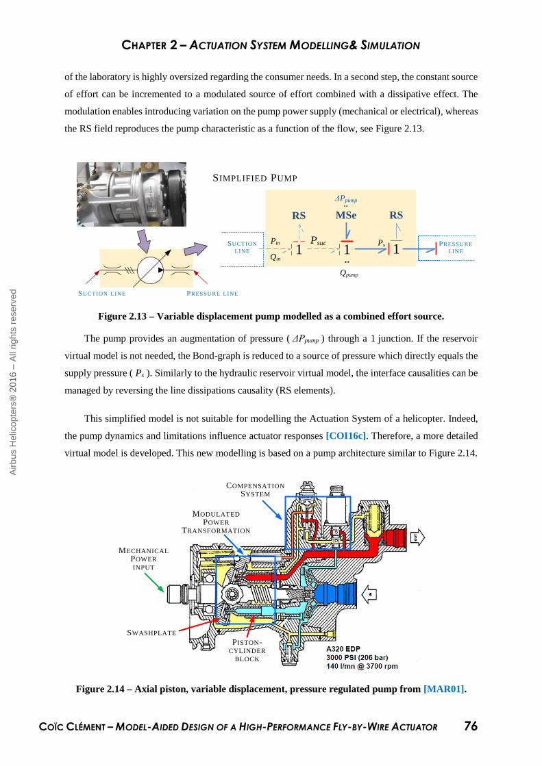
CHAPTER 2 – ACTUATION SYSTEM MODELLING& SIMULATION
COÏC CLÉMENT – MODEL-AIDED DESIGN OF A HIGH-PERFORMANCE FLY-BY-WIRE ACTUATOR 76
of the laboratory is highly oversized regarding the consumer needs. In a second step, the constant source
of effort can be incremented to a modulated source of effort combined with a dissipative effect. The
modulation enables introducing variation on the pump power supply (mechanical or electrical), whereas
the RS field reproduces the pump characteristic as a function of the flow, see Figure 2.13.
MSe
1Pin
Qin
SIMPLIFIED PUMP
RS
1SUCTION
LINE
ΔPpump ..
..
Qpump
RS
1Psuc Ps PRESSURE
LINE
PRESSURE LINESUCTION LINE
Figure 2.13 – Variable displacement pump modelled as a combined effort source.
The pump provides an augmentation of pressure ( ΔPpump ) through a 1 junction. If the reservoir
virtual model is not needed, the Bond-graph is reduced to a source of pressure which directly equals the
supply pressure ( Ps ). Similarly to the hydraulic reservoir virtual model, the interface causalities can be
managed by reversing the line dissipations causality (RS elements).
This simplified model is not suitable for modelling the Actuation System of a helicopter. Indeed,
the pump dynamics and limitations influence actuator responses [COI16c]. Therefore, a more detailed
virtual model is developed. This new modelling is based on a pump architecture similar to Figure 2.14.
MECHANICAL POWER
INPUT
MODULATED POWER
TRANSFORMATION
COMPENSATION
SYSTEM
SWASHPLATE
PISTON-CYLINDER
BLOCK
Figure 2.14 – Axial piston, variable displacement, pressure regulated pump from [MAR01].
Airb
us H
elic
opte
rs®
2016 –
All
rights
reserv
ed

CHAPTER 2 – ACTUATION SYSTEM MODELLING& SIMULATION
COÏC CLÉMENT – MODEL-AIDED DESIGN OF A HIGH-PERFORMANCE FLY-BY-WIRE ACTUATOR 77
In such a pump architecture, mechanical power drives a shaft that rotates a cylinder block. In this
block, several pistons are guided in a parallel direction with regard to the drive shaft. All pistons are
linked to a swashplate by a spherical fluid bearing connection called piston shoe. Piloting the swashplate
angle allows modulating the piston strokes inside the cylinder block. Fluid is sucked from the inlet with
a flowrate function of the rotation speed and the swashplate angle (and thus the cylinder displacements).
In one block rotation, the reduction of piston-cylinder volumes, due to the piston displacement,
compresses the contained fluid, thus providing a pressurized flow rate to the hydraulic system. The
compensation system is composed of a regulator valve and a displacement actuator. The regulator valve
compares the output pressure with a reference pressure (usually set by a spring) and modulates hydraulic
power to the displacement actuator, which acts on the swashplate angle.
One way to model this pump is to consider that the piston-cylinders act as several modulated power
transformers (MTF element) from the mechanical to the hydraulic domain, the transformation ratios of
which equal the cylinder displacements relative to the shaft rotation. The flow source in the mechanical
domain, the angular speed ωshaft, becomes a volume flow rate Qpump that is propagated to the suction and
delivering lines through a 1 junction. In the delivering line, the flow is compressed by a C element. The
compensation system is modelled as a simple first order dynamic with saturations which modulates the
MTF elements.
Note 2.6: The compensation saturation shall be placed on the integral itself (and not after) in order
to avoid unrealistic delays when leaving the saturation. To do so, it is necessary to write the first order
in its canonical form. This also allows introducing speed saturation before the integral.
In nominal operation, the internal leakage is functional. It allows the generated heat and pollution13
to be evacuated and is used as a fluid bearing in some parts such as piston shoes. Usually, the internal
leakage outlet is the drain. Therefore, the internal leakage is herein modelled as an MRS-field dissipating
hydraulic power to the drain, seen as a pump interface. With the increase of wear, the internal leakage
also increases. It is herein optionally modelled as a single, entirely dissipated, loss of flow at the pump
high pressure. Leakage evolution is controllable through the triggering input, as an extension of the
model from [MAR01].
13 Quantification of the fluid pollution is not addressed in this model.
Airb
us H
elic
opte
rs®
2016 –
All
rights
reserv
ed

CHAPTER 2 – ACTUATION SYSTEM MODELLING& SIMULATION
COÏC CLÉMENT – MODEL-AIDED DESIGN OF A HIGH-PERFORMANCE FLY-BY-WIRE ACTUATOR 78
RS
K1+τs
C1
MRS
PUMP MODEL FOR
EQUIPMENT INTEGRATOR
MECHANICAL POWER
INPUT
SUCTION LINE
PRESSURE LINE
FAULT TRIGGERING
INTERNAL LEAKAGE
Qin
ΔPpump
PRESSURE LINE
SUCTION LINE
MECHANICAL POWER
INPUTMTF : Qpump1
0
FAULT TRIGGERING
REGULATION DEFICIENCY
Pref
De
DRAIN
1
RS 1
Pin
Qout Pout
Figure 2.15 – Virtual Model: axial piston, variable displacement, pressure-regulated pump.
Another possible fault that has been modelled is regulation system deficiency. It can be either
progressive, leading to a slower regulation dynamic, or instantaneous. It usually ends with a constant
angle of the swashplate (the pump becomes thus a fixed displacement pump). Both cases can be
triggered with the signal arrows using real or Boolean input respectively.
The pump virtual model developed in this PhD dissertation for virtual integration of the Actuation
System is presented in Figure 2.15. As a simplification, a single modulated transformer is used to
represent an equivalent cylinder block which compresses the fluid in an equivalent chamber.
Consequently, this model does not allow simulating the dynamic of each piston and the associated
pressure and flow ripples.
It is relevant to note that such a model is detailed enough for most Airbus Helicopters simulations,
but too simplified for pump manufacturers. It is then important to know that more detailed models exist,
for example [VEL03] modelled vane pumps using multi-Bonds. These models could be used for our
simulation needs, but the dynamics involved would dramatically slow down the simulation and the
parameters needed by the models are usually not available for integrators at early phases of the
development.
Airb
us H
elic
opte
rs®
2016 –
All
rights
reserv
ed

CHAPTER 2 – ACTUATION SYSTEM MODELLING& SIMULATION
COÏC CLÉMENT – MODEL-AIDED DESIGN OF A HIGH-PERFORMANCE FLY-BY-WIRE ACTUATOR 79
3.3.3. Hydraulic Power Distribution Virtual Model
Hydraulic power coming from the power generation is distributed to the consumers through a
sophisticated hydraulic circuit which was designed based on the safety requirements and includes
several by-pass valves, check valves, filters, pipes…
In an early development phase, the architecture of the hydraulic power distribution and the routing
of the pipe are not known. But a good estimation of the pressure losses ( ΔP ) – which depend on the
volume flow rate ( Q ) – is needed to assess the impact on actuator performance. The overall Actuation
System virtual model shall be accurate but conservative in terms of performance. This means that the
physical model shall at least have the same performances as the one simulated. The consequence for the
hydraulic power distribution virtual model is that the pressure losses shall not be underestimated.
Therefore, it is suggested herein to design a simplified hydraulic power distribution network which
represents the main pressure losses. These are considered as local or distributed (but modelled as lumped
effect) pressure losses. Both dissipative effects are modelled in Bond-graphs with an RS element, but
the equations linking the effort and the flow variables depend on the flow pattern and the type of
hydraulic restriction.
3.3.3.1. Flow Patterns
Flow patterns can be either laminar, turbulent or in transition. In a laminar flow pattern, the flow
rate is mainly constrained by the viscous friction of the fluid. Speed vectors of neighbourhood fluid
particles tend to be parallel and oriented in the flow direction [FAI83]. By contrast, a turbulent flow
pattern is characterized by the inertia forces of the fluid. Speed vectors of all particles tend to diverge
from the flow direction [GUI92].
The transition domain is still neither well-known nor well-defined in the literature. This can be
explained as it has been experimentally shown that the restriction shape highly impacts the value of the
transition. However, the transition range is quite small relative to the Reynolds number values that can
be reached. Therefore, the transition is usually considered as a point (and no longer a range) called the
critical Reynolds number. The hysteresis effect in the transition domain is thus neglected.
The Reynolds number ( Re ) [REY86] characterizes the type of flow pattern. It is given by
Equation 2.5 for circular14 flow sections.
4e
vDR Q
D
Equation 2.5
14 If the flow section is not circular, the “hydraulic diameter” provides genericity to this formula by defining an
equivalent diameter regardless of the shape of the flow section. It is not used in this dissertation.
Airb
us H
elic
opte
rs®
2016 –
All
rights
reserv
ed

CHAPTER 2 – ACTUATION SYSTEM MODELLING& SIMULATION
COÏC CLÉMENT – MODEL-AIDED DESIGN OF A HIGH-PERFORMANCE FLY-BY-WIRE ACTUATOR 80
where:
v is the fluid velocity, [m/s]
υ is the kinematic viscosity, [m²/s]
D is the pipe or orifice diameter, [m]
Equation 2.5 is applied to pipes or orifices, which are the main components used in the Actuation
Systems that require Reynolds number calculation. The Reynolds number is a positive15 dimensionless
relation that represents the ration between the inertial forces and viscous forces. Sufficiently low
Reynolds numbers correspond to a laminar flow, while sufficiently high values are for a turbulent flow
pattern.
It is important to note that calculating the Reynolds number requires the volume flow rate. It is then
convenient to express the pressure losses as a function of the volume flow rate:
2 2
22 2e eR R
Q vP sign Q sign v
Equation 2.6
Even if a square root appears in Equation 2.6, the flow pattern is not necessarily turbulent. Indeed,
the pressure drop coefficient16 ξ is dependent on the flow pattern and thus on the Reynolds number. In
case of a laminar flow, the pressure drop coefficient has the Reynolds number at the denominator,
leading thus to a linear relation between the volume flow rate and the pressure losses. Expressions of
this coefficient are given in the two following sections.
Respecting this causality of the equation constrains the causality of the bond linked to the R element
in order to avoid an algebraic loop. The flow number ( λ ) has been created conveniently [CLO80] to
permit the other causality without generating an algebraic loop.
2 PD
Equation 2.7
The flow number is obtained by substituting the expression of the flow rate in the Reynolds number
expression. This leads to a new equation linking the Reynolds number, the flow number and the
restriction coefficient. The flow coefficient ( cq ) is an image of the pressure drop coefficient in the
inverse causality, i.e. volume flow rate function of pressure losses. It is a conductance coefficient.
e qR c
Equation 2.8
15 Even if the well-known expression of the Reynolds number does not include the absolute value of the speed or
volume flow rate, it is usual to plot its values in a logarithmic scale, requiring a positive flow or speed. 16 The pressure drop coefficient is also called “resistance coefficient” in the literature, e.g. [IDE66].
Airb
us H
elic
opte
rs®
2016 –
All
rights
reserv
ed

CHAPTER 2 – ACTUATION SYSTEM MODELLING& SIMULATION
COÏC CLÉMENT – MODEL-AIDED DESIGN OF A HIGH-PERFORMANCE FLY-BY-WIRE ACTUATOR 81
Once the flow number has been introduced, it is possible to select the right flow coefficient without
any algebraic loop and thus compute the volume flow rate using Equation 2.9.
2( )qQ c P sign P
Equation 2.9
These principles have been presented herein with a focus on causality aspects in order to facilitate
further software implementation for simulation. This is not necessarily done in a chronological order. In
fact, it depends on regional conventions if Equation 2.6 or Equation 2.9 is used.
3.3.3.2. Local Pressure Losses
Local pressure losses occur in almost any change of shape in the hydraulic line: hydraulic fittings,
pipe bend angles, valves, etc. These restrictions can be classified into fixed and variable restrictions.
On one side, the causality on fixed restrictions is “free”. However, the literature usually presents
the parameters characterizing many local restrictions using the pressure drop coefficient ( ξ ), e.g.
[IDE66] [GUI92]. Therefore, Equation 2.6 would be preferred as it becomes easier to provide the
parameters (requirement R8).
On the other side, some variable restrictions can be fully closed, which leads to a zero flow section,
e.g. a poppet valve. In order to avoid division by zero, it is preferable to reverse the causality using the
flow coefficient and thus Equation 2.9.
Figure 2.16 synthesizes the preferred causalities for each type of restriction based on equations
found in the literature and implementation constraints as detailed above.
RS
1
MRS
1
(a) – Fixed restrictions (b) – Variable restrictions
Figure 2.16 – Preferred restriction causalities based on equations found in literature.
Any change of shape in the distribution system disturbs the flow lines. As a consequence, a flow
pattern in singularities becomes rapidly turbulent. This is equivalent to low transition Reynolds numbers
or flow numbers. For example, in case of an orifice (small length compared to its diameter), transition
can occur for Reynolds numbers between 15 and 240 [GUI92]. The critical Reynolds number is usually
considered equal to 100 in our application. In the next section, values of critical Reynolds numbers are
given for pipes.
Airb
us H
elic
opte
rs®
2016 –
All
rights
reserv
ed

CHAPTER 2 – ACTUATION SYSTEM MODELLING& SIMULATION
COÏC CLÉMENT – MODEL-AIDED DESIGN OF A HIGH-PERFORMANCE FLY-BY-WIRE ACTUATOR 82
Figure 2.17 – Flow coefficient evolution with the Reynolds number, from [TCH79].
Sensitivity of the volume flow rate to temperature through orifices is studied in section 3.4.4
dedicated to valve modelling. A particular case of restriction, where the transition from laminar to
turbulent is functional and managed by design, is presented in Chapter 3: the short tube orifice. This has
also been presented in a paper [COI16a] at the International Conference on Hydraulics and Pneumatics
(Praha, Czech Republic). This paper had been selected as the opening keynote of the conference.
3.3.3.3. Distributed Pressure Losses
Distributed pressure losses occur when the flow goes through a hydraulic line with a length (without
any major change of shape) that is much higher than its diameter. This is mainly the case for rigid pipes
and hoses with low curving in the hydraulic power distribution. Both will be referred to as pipes or
hydraulic lines in this dissertation, unless otherwise specified. However, the parameters provided to the
virtual models will depend on the nature of the hydraulic line.
Equation 2.6 models these flow patterns in a lumped parameter manner, taking into account that
the pressure drop coefficient equals a friction factor times the length to diameter ratio of the pipe:
Lf
D Equation 2.10
where:
f is the friction factor, [-]
L is the pipe length, [m]
In pipes, the pressure losses are modelled by the Hagen-Poiseuille equation for laminar flow
patterns. However, this modelling does not include the perturbations at the pipe entrance and exit or the
length needed to establish the laminar flow after such perturbations. Therefore, a general expression is
used for pipes that are longer than the establishment length:
64in est out
e
L
R D Equation 2.11
Airb
us H
elic
opte
rs®
2016 –
All
rights
reserv
ed

CHAPTER 2 – ACTUATION SYSTEM MODELLING& SIMULATION
COÏC CLÉMENT – MODEL-AIDED DESIGN OF A HIGH-PERFORMANCE FLY-BY-WIRE ACTUATOR 83
where:
64/Re is the friction factor providing the Hagen-Poiseuille equation, [-]
𝜉in is the pressure drop coefficient representing local entrance losses, [-]
𝜉est is the pressure drop coefficient representing the establishment length, [-]
𝜉out is the pressure drop coefficient representing local output losses. [-]
Typical values for 𝜉in, 𝜉est and 𝜉out can be found for example in [IDE66] [MER67] [GUI92].
For turbulent flow patterns, input and output perturbation and establishment length are negligible.
Blasius experimentally defined the friction factor for turbulent flow patterns with Reynolds numbers
below 105 and Prandtl’s determined a universal law that is difficult to manage mathematically [MER67].
Nikuradse linked the friction factor with the pipe roughness for turbulent flow patterns [NIK33].
Based on a study conducted with Airbus Helicopters data, it is affirmed herein that in pipes of our
hydraulic power distribution network, admissible velocities correspond to a Reynolds number for which
the Blasius equation is always applicable in case of turbulent flow. As listed in [SAE12], fluid velocity
limitations should be identified taking into account:
“Allowable pressure drop at minimum required operating temperatures.
Pressure surges caused by high fluid velocity and fast response valves.
Back pressure in return lines, as it may affect brakes and pump case drain lines.
Pump inlet pressure, as affected by long suction lines and a high response rate variable volume
pump.”
Regarding the laminar to turbulent transition, Osborne Reynolds wrote in [REY86] that a laminar
flow pattern occurs for Reynolds numbers below 1400. Herbert E. Merritt defined a transition range
from 2000 to 4000 [MER67]. Jacques Faisandier considered that this range could be from 1000 to 2300
[FAI83].
With the aim of being conservative on the pressure loss calculation, the critical Reynolds number
for pipes has been determined as the intersection between the Hagen-Poiseuille and Blasius asymptotes.
Such intersection occurs when the Reynolds number equals 1187, which gives a friction factor f of 0.054.
With this value for the critical Reynolds number, it is ensured that the friction factor considered is always
the highest value of those given by the Hagen-Poiseuille and Blasius equations. Figure 2.18 synthesizes
the previously detailed information.
Airb
us H
elic
opte
rs®
2016 –
All
rights
reserv
ed
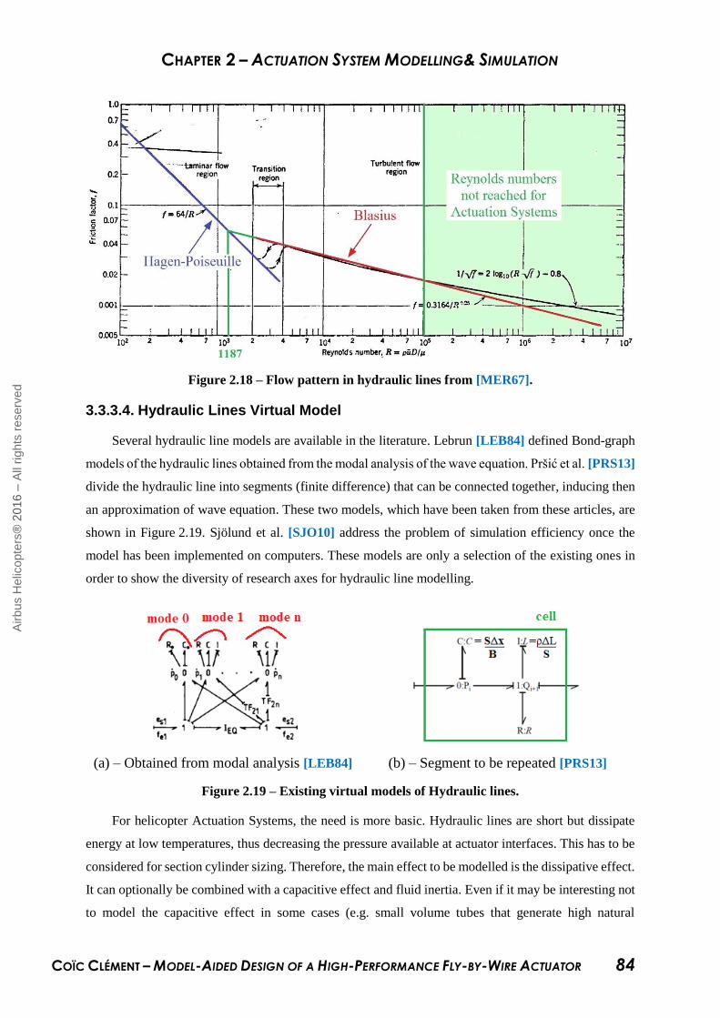
CHAPTER 2 – ACTUATION SYSTEM MODELLING& SIMULATION
COÏC CLÉMENT – MODEL-AIDED DESIGN OF A HIGH-PERFORMANCE FLY-BY-WIRE ACTUATOR 84
Figure 2.18 – Flow pattern in hydraulic lines from [MER67].
3.3.3.4. Hydraulic Lines Virtual Model
Several hydraulic line models are available in the literature. Lebrun [LEB84] defined Bond-graph
models of the hydraulic lines obtained from the modal analysis of the wave equation. Pršić et al. [PRS13]
divide the hydraulic line into segments (finite difference) that can be connected together, inducing then
an approximation of wave equation. These two models, which have been taken from these articles, are
shown in Figure 2.19. Sjölund et al. [SJO10] address the problem of simulation efficiency once the
model has been implemented on computers. These models are only a selection of the existing ones in
order to show the diversity of research axes for hydraulic line modelling.
(a) – Obtained from modal analysis [LEB84] (b) – Segment to be repeated [PRS13]
Figure 2.19 – Existing virtual models of Hydraulic lines.
For helicopter Actuation Systems, the need is more basic. Hydraulic lines are short but dissipate
energy at low temperatures, thus decreasing the pressure available at actuator interfaces. This has to be
considered for section cylinder sizing. Therefore, the main effect to be modelled is the dissipative effect.
It can optionally be combined with a capacitive effect and fluid inertia. Even if it may be interesting not
to model the capacitive effect in some cases (e.g. small volume tubes that generate high natural
Airb
us H
elic
opte
rs®
2016 –
All
rights
reserv
ed

CHAPTER 2 – ACTUATION SYSTEM MODELLING& SIMULATION
COÏC CLÉMENT – MODEL-AIDED DESIGN OF A HIGH-PERFORMANCE FLY-BY-WIRE ACTUATOR 85
frequencies), in most applications, the capacitance is used to add a state variable and thus to compute
the pipe pressure. According to the needs of Airbus Helicopters, inertia is rarely modelled. However, it
is required when modelling the line dynamics (for other applications such as fluid injection or
investigation of the “water hammer effect”).
RS
1
I
C
0Pin
Qin Qout
Qcomp
Pout INLET OUTLET
RS
1
C
0Pin
Qin Qout
Qcomp
Pout INLET OUTLET
(a) – RIC model (b) – RC model requiring the use of the flow number
Figure 2.20 – Pipe virtual model used in our Actuation System modelling.
Causality on the RS element is dependent on the modelled effects. As detailed above, it is
convenient to use the pressure drop coefficient in the pipe model. Therefore, causality on the RS-element
is preferable to receive the flow variable and provide the pressure losses to the 1 junction. However, if
inertial forces are not modelled, the causality on the dissipative effect must be modified in order to keep
the same interfaces and to conserve the integral causality on the capacitive effect (preferred for
simulation). Then the flow number is used in combination with Equation 2.9.
Note 2.7: The volume flow rate calculation from the “enriched” Hagen-Poiseuille equation – as
defined in Equation 2.11 – would need polynomial solving if the establishment length were considered.
This concludes the hydraulic power distribution virtual model. The next section is dedicated to the
main consumers of interest for the Actuation System: the primary flight control actuator virtual model.
3.4. FbW Actuator Virtual Model
There are many actuators on helicopters, but within the scope of this thesis they can all be neglected
except for hydraulically powered actuators. Therefore, in this dissertation, the term actuator refers
exclusively to hydraulic actuators (including electro-hydraulic and hydro-mechanical actuators).
FbW actuators are considered as main consumers of the hydraulic power generation and
distribution systems. This does not mean that they consume more power than other equipment. Indeed,
on many helicopters, landing gears or military equipment such as harpoons or sonars are more
demanding in terms of instantaneous volume flow rate. But these demands are limited to a short period
of time and associated with lower criticality. In contrast, actuators are in permanent motion to satisfy
pilot and autopilot orders.
Airb
us H
elic
opte
rs®
2016 –
All
rights
reserv
ed

CHAPTER 2 – ACTUATION SYSTEM MODELLING& SIMULATION
COÏC CLÉMENT – MODEL-AIDED DESIGN OF A HIGH-PERFORMANCE FLY-BY-WIRE ACTUATOR 86
The actuator virtual model is divided into the same subsystems that have been suggested in
Figure 1.15 of Chapter 1. This coherence satisfies requirement R1 of the modelling needs, thus
facilitating incremental modelling.
It has been preferred to first detail the cylinder virtual model as it can be used for the EHSV virtual
model for example. Then, as part of the control module, the interface, pilot and power modulation stages
are described. Finally, the closed loop virtual model is presented.
3.4.1. Cylinder Virtual Model
In this dissertation, the cylinder, also called piston-cylinder assembly in the literature, refers to
double effect cylinders. As mentioned above, primary flight control actuators are redundant and thus
usually include two cylinders which are geometrically associated in series or in parallel. Only one
cylinder is detailed in this section as the second one would be identical.
From a mechanical point of view, only two degrees of freedom are relevant: the axial displacement
along the rod axis and the rotation around the eye-end necessary for the swashplate kinematic. The
standardized mechanical components are then used to connect bodies and interface as “plug and play”
components. The mechanical quadriport provides a high added value as both degrees of freedom are
modelled in it.
With regard to the hydraulic interfaces, the cylinder has two connections with the control module
in order to receive the fluid going to one chamber or deliver the fluid ejected by the other chamber. By
convention, the positive volume flow is the flow entering the chambers.
The cylinder is virtually split into two parts: the extension side, relative to the extension chamber,
and analogically the retraction side. Subscripts “ext” and “ret” respectively refer to the extension and
retraction sides.
In each chamber, the flow coming from the EHSV valve is either compressed (subscript “c”), as
required for piston displacement (subscript “d”), or optionally leaked (subscript “L”) from the chambers
to the atmosphere or between chambers through the piston (subscript “pist”).
Note 2.8: The leakage can be dependent on the piston-rod/housing cylinder assembly. This
dependence is not shown in Figure 2.21 for readability reasons but is necessary for modelling fluid
bearings (see Chapter 3).
Airb
us H
elic
opte
rs®
2016 –
All
rights
reserv
ed
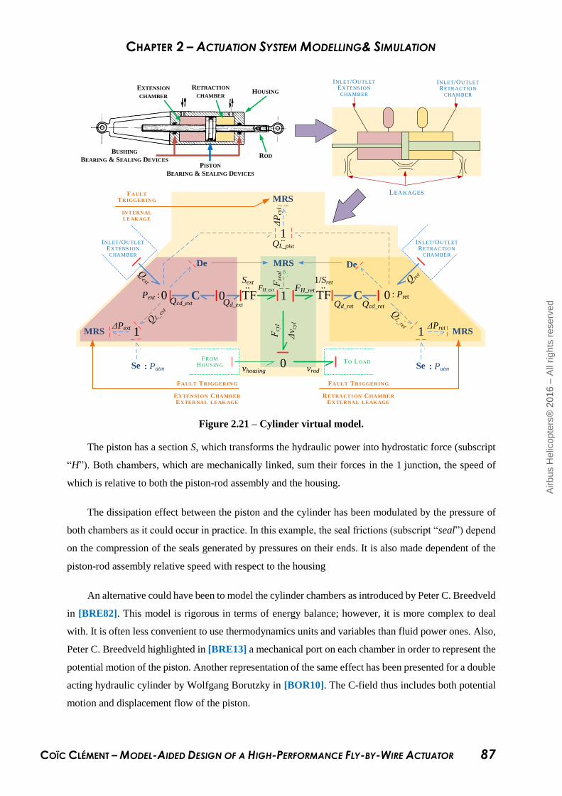
CHAPTER 2 – ACTUATION SYSTEM MODELLING& SIMULATION
COÏC CLÉMENT – MODEL-AIDED DESIGN OF A HIGH-PERFORMANCE FLY-BY-WIRE ACTUATOR 87
INLET/OUTLET
RETRACTION CHAMBER
INLET/OU TLET
EXTENS I ON CHAMBER
0Qcd_ext
Pext : TFFH_ext
1C
Sext..
1
FH_ret 0
Qd_ret : Pret TF
1/Sret..
1
0 vrod vhousing
FROM
HOUS INGTO LO AD
MRSΔPext
MRSΔPret
1
MRS
ΔP
cyl
MRS
FAULT TR IGGER IN G
IN TERN AL LEAK AGE
Se : Patm Se : Patm
FAULT TRIGGERING
RETRACTI ON CHAMBER
EXTERNAL LEAK AGE
FAULT TRIGGERING
EXTENSI ON CHAMBER
EXTERNAL LEAK AGE
..QL_pist
PISTON
BEARING & SEALING DEVICES
BUSHING
BEARING & SEALING DEVICESROD
HOUSINGEXTENSION
CHAMBER
RETRACTION
CHAMBER
INLET/OUTLET
EXTENS I ON CHAMBER
INLET/OUTLET
RETRA CTIO N CHAMBER
LEA KAGES
De De
Qd_ext 0 C
Qcd_ret
Figure 2.21 – Cylinder virtual model.
The piston has a section S, which transforms the hydraulic power into hydrostatic force (subscript
“H”). Both chambers, which are mechanically linked, sum their forces in the 1 junction, the speed of
which is relative to both the piston-rod assembly and the housing.
The dissipation effect between the piston and the cylinder has been modulated by the pressure of
both chambers as it could occur in practice. In this example, the seal frictions (subscript “seal”) depend
on the compression of the seals generated by pressures on their ends. It is also made dependent of the
piston-rod assembly relative speed with respect to the housing
An alternative could have been to model the cylinder chambers as introduced by Peter C. Breedveld
in [BRE82]. This model is rigorous in terms of energy balance; however, it is more complex to deal
with. It is often less convenient to use thermodynamics units and variables than fluid power ones. Also,
Peter C. Breedveld highlighted in [BRE13] a mechanical port on each chamber in order to represent the
potential motion of the piston. Another representation of the same effect has been presented for a double
acting hydraulic cylinder by Wolfgang Borutzky in [BOR10]. The C-field thus includes both potential
motion and displacement flow of the piston.
Airb
us H
elic
opte
rs®
2016 –
All
rights
reserv
ed
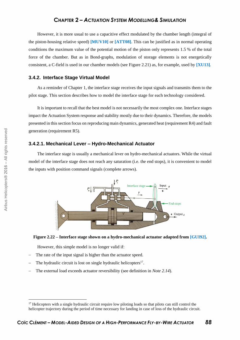
CHAPTER 2 – ACTUATION SYSTEM MODELLING& SIMULATION
COÏC CLÉMENT – MODEL-AIDED DESIGN OF A HIGH-PERFORMANCE FLY-BY-WIRE ACTUATOR 88
However, it is more usual to use a capacitive effect modulated by the chamber length (integral of
the piston-housing relative speed) [MUV10] or [ATT08]. This can be justified as in normal operating
conditions the maximum value of the potential motion of the piston only represents 1.5 % of the total
force of the chamber. But as in Bond-graphs, modulation of storage elements is not energetically
consistent, a C-field is used in our chamber models (see Figure 2.21) as, for example, used by [XU13].
3.4.2. Interface Stage Virtual Model
As a reminder of Chapter 1, the interface stage receives the input signals and transmits them to the
pilot stage. This section describes how to model the interface stage for each technology considered.
It is important to recall that the best model is not necessarily the most complex one. Interface stages
impact the Actuation System response and stability mostly due to their dynamics. Therefore, the models
presented in this section focus on reproducing main dynamics, generated heat (requirement R4) and fault
generation (requirement R5).
3.4.2.1. Mechanical Lever – Hydro-Mechanical Actuator
The interface stage is usually a mechanical lever on hydro-mechanical actuators. While the virtual
model of the interface stage does not reach any saturation (i.e. the end stops), it is convenient to model
the inputs with position command signals (complete arrows).
Figure 2.22 – Interface stage shown on a hydro-mechanical actuator adapted from [GUI92].
However, this simple model is no longer valid if:
The rate of the input signal is higher than the actuator speed.
The hydraulic circuit is lost on single hydraulic helicopters17.
The external load exceeds actuator reversibility (see definition in Note 2.14).
17 Helicopters with a single hydraulic circuit require low piloting loads so that pilots can still control the
helicopter trajectory during the period of time necessary for landing in case of loss of the hydraulic circuit.
Airb
us H
elic
opte
rs®
2016 –
All
rights
reserv
ed

CHAPTER 2 – ACTUATION SYSTEM MODELLING& SIMULATION
COÏC CLÉMENT – MODEL-AIDED DESIGN OF A HIGH-PERFORMANCE FLY-BY-WIRE ACTUATOR 89
Indeed, these conditions would make the mechanical lever reach its end-stops on the actuator
housing. Then, the input does no longer provide a position but an effort command to the actuator. It
should therefore be modelled by a mechanical bond.
Mechanical kinematics of the interface stage highly depends on the actuator. In addition, this
dissertation focuses on FbW technologies. Therefore, even though it has been judged necessary to clarify
the type of input on hydro-mechanical actuators, no particular virtual model of the interface stage is
presented in this dissertation for these actuators.
3.4.2.2. Electric Motor – DDV- and EHSV-Based Actuator
The interface stage of a DDV-based actuator is composed of several LAT motors. EHSV also
includes LAT motors but usually is referred to as “coils”. Therefore, both technologies will have the
same interface stage model even if parameters will differ.
Each motor is mechanically interfaced with the housing and its pilot stage through the stator
(subscript “stat”) and rotor (subscript “rot”), respectively (also see Figure 2.4 for the topology of the
DDV). Benefit is taken from standardized mechanical components, so both the stator and the rotor are
modelled with a standardized mechanical body. In Figure 2.23, only the rotations around the rotor axis
are shown as there are the functional motions of the motors. However, standardized mechanical bodies
allow subsequent upgrading of the model for translation in the rotor axis direction if required (e.g. for a
vibration study, which is relevant in a helicopter environment).
GY1
I : Lmot_i
Udown
Idown
Uup
Iup
MRS : Rmot_i
FAULT TRIGGERING
OPEN CIRCUIT
0
0
MRSFAULT
TRIGGERING
SHORT CIRCUIT
0 MRS
FAULT TRIGGERING
MOTOR SEIZING
JROTEMF
UPSTREAM
DOWNSTREAM
ROTORSTATOR
1
UPSTREAM
DOWNSTREAMHOUSING
PILOT
STAGE1
IJrot_i :
1
IJstat_i :
0C
Figure 2.23 – Interface stage: electrical motor virtual model.
Airb
us H
elic
opte
rs®
2016 –
All
rights
reserv
ed

CHAPTER 2 – ACTUATION SYSTEM MODELLING& SIMULATION
COÏC CLÉMENT – MODEL-AIDED DESIGN OF A HIGH-PERFORMANCE FLY-BY-WIRE ACTUATOR 90
The interface between stator and rotor is usually the motor housing: the stator is fixed on the
housing, which is linked to the rotor via hinges. Thus only one degree of freedom is left to the rotor –
the rotation around its axis. It is simplified herein for readability and implementation reasons. The stator
and rotor are optionally linked with a 0 junction that includes an MRS element. It represents the friction
between both mechanical bodies. An increase of such friction leads to motor seizing.
Note 2.9: This interface is a highly simplified standardized mechanical interface but still shows the
genericity of the proposed standardization.
In the mechanical domain, the cogging torque is equivalent to a non-linear elastic effect that
depends on the relative angular position of the rotor and stator. Therefore, it is modelled as a C element
in this Figure 2.23.
From an electrical point of view, the (permanent magnet) LAT motor is modelled as an equivalent
DC motor. The model is based on physical topology. The upstream and downstream wirings are
connected to a 1 junction, representing a serial circuit, on which the inductance, resistance and electro-
magnetic force are respectively modelled with I (Lmot), MRS (Rmot) and the GY elements. In addition,
electrical faults can be triggered. The short circuit corresponds to a low resistance between both wirings.
Strongly increasing the resistance in the serial circuit opens the circuit.
Note 2.10: The causality on the MRS modelling motor resistance (Rmot) is reversed regarding the
preferred causalities detailed in Figure 2.16 for hydraulics. However, the analogy should be perfect
between both the hydraulic and the electric domains. This difference is reasonable as the resistance is
not tending to zero but to infinity. Thus, there is no risk of dividing by zero.
More detailed models are available in the literature, e.g. [ROM00] [XU13]. They include for
example magnetic effects. But the increased complexity is not needed for our purposes and parameters
can result more difficult to be obtained for an integrator such as Airbus Helicopters.
On NH90 actuators, the interface stage is composed of four LAT motors, whereas several coils are
used for the EHSV-based actuators (usually three). Such redundancy can either be represented in an
object-oriented way by instantiating the same motor model several times or by using multi Bond-graphs
and connecting them to a standardized mechanical body. Their connection will not create a causality
conflict as the standardized mechanical body is thought to connect several standardized interfaces.
3.4.3. Pilot Stage Virtual Model
The pilot stage drives the power modulation stage from the output of the interface stage. For the
same reasons as for the interface stage, no particular model of the hydro-mechanical actuator is presented
Airb
us H
elic
opte
rs®
2016 –
All
rights
reserv
ed
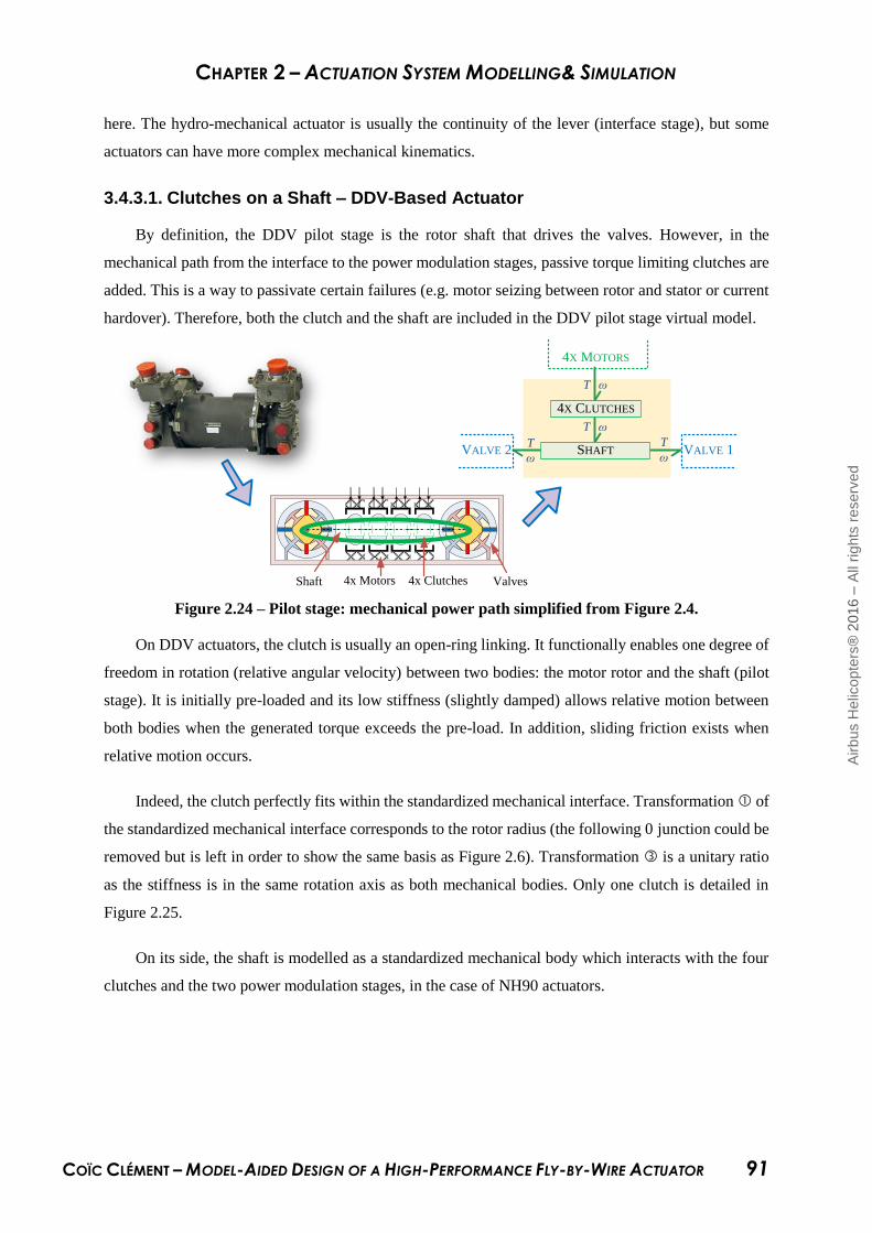
CHAPTER 2 – ACTUATION SYSTEM MODELLING& SIMULATION
COÏC CLÉMENT – MODEL-AIDED DESIGN OF A HIGH-PERFORMANCE FLY-BY-WIRE ACTUATOR 91
here. The hydro-mechanical actuator is usually the continuity of the lever (interface stage), but some
actuators can have more complex mechanical kinematics.
3.4.3.1. Clutches on a Shaft – DDV-Based Actuator
By definition, the DDV pilot stage is the rotor shaft that drives the valves. However, in the
mechanical path from the interface to the power modulation stages, passive torque limiting clutches are
added. This is a way to passivate certain failures (e.g. motor seizing between rotor and stator or current
hardover). Therefore, both the clutch and the shaft are included in the DDV pilot stage virtual model.
4x Motors 4x Clutches ValvesShaft
T ω
T ω
T
ω
T
ω VALVE 2
4X MOTORS
4X CLUTCHES
SHAFT VALVE 1
Figure 2.24 – Pilot stage: mechanical power path simplified from Figure 2.4.
On DDV actuators, the clutch is usually an open-ring linking. It functionally enables one degree of
freedom in rotation (relative angular velocity) between two bodies: the motor rotor and the shaft (pilot
stage). It is initially pre-loaded and its low stiffness (slightly damped) allows relative motion between
both bodies when the generated torque exceeds the pre-load. In addition, sliding friction exists when
relative motion occurs.
Indeed, the clutch perfectly fits within the standardized mechanical interface. Transformation of
the standardized mechanical interface corresponds to the rotor radius (the following 0 junction could be
removed but is left in order to show the same basis as Figure 2.6). Transformation is a unitary ratio
as the stiffness is in the same rotation axis as both mechanical bodies. Only one clutch is detailed in
Figure 2.25.
On its side, the shaft is modelled as a standardized mechanical body which interacts with the four
clutches and the two power modulation stages, in the case of NH90 actuators.
Airb
us H
elic
opte
rs®
2016 –
All
rights
reserv
ed

CHAPTER 2 – ACTUATION SYSTEM MODELLING& SIMULATION
COÏC CLÉMENT – MODEL-AIDED DESIGN OF A HIGH-PERFORMANCE FLY-BY-WIRE ACTUATOR 92
CL
UT
CH
1
FROM MOTOR ROTOR 1
SHAFT
0
TR1 ωR1
1
TF
TF 0
0
MRS
1 MRSCFree-play
/ Wear
De
0THERMAL
MODEL
Dilatation
Stiffness Damping
Friction losses
NORMAL
AXIS
TANGENTIAL
AXIS
1 I : JSHAFT
CLUTCH 2
CLUTCH 3
CLUTCH 4
TO POWER MODULATION STAGES
TC1 ωC1
CLUTCH 1
Figure 2.25 – DDV pilot stage virtual model: clutches and shaft.
Note 2.11: This clutch modelling implies that, even if it is a mechanical part, it has been chosen to
model it as an interface. This makes sense as no inertial effect of the open-ring is required but
compliance and friction effects are of interest.
3.4.3.2. Hydraulic Potentiometer Piloting the Spool Faces – EHSV-Based Actuator
On EHSV, the pilot stage18 can be seen as a hydraulic potentiometer. It acts on the pressures
available at the spool faces. Two19 main technologies (Figure 2.26) exist for hydraulic potentiometers:
the double flapper-nozzle. It consists of a movable flapper that varies the restriction at the nozzle
outlets (see Figure 2.26-(a)).
the jet-pipe. It consists of a movable jet with two collector holes that direct fluid to one or the other
end faces of the spool [THO90], (see Figure 2.26-(b)).
18 On EHSV, the pilot stage is usually called first stage. The term pilot stage is introduced in this dissertation for
reasons of genericity, independently of the technology. 19 The jet deviator can be seen as a variant of the jet-pipe.
Airb
us H
elic
opte
rs®
2016 –
All
rights
reserv
ed

CHAPTER 2 – ACTUATION SYSTEM MODELLING& SIMULATION
COÏC CLÉMENT – MODEL-AIDED DESIGN OF A HIGH-PERFORMANCE FLY-BY-WIRE ACTUATOR 93
PILOT STAGES
INTERFACE STAGES
POWER MODULATION STAGES
(a) – Double Flapper-Nozzle [MOO14] (b) – Jet-pipe
(c) – Double Flapper-Nozzle model [MAR93] (d) – Jet-pipe model [THO90]
Figure 2.26 – EHSV technologies and their pilot stage models.
In aerospace applications, jet-pipes are preferred for their lower leakage and sensitivity to fluid
pollution. Unfortunately, jet pipes are complex to model (and to design). Some models are available:
Thoma wrote the continuity and momentum equations and converted them into a Bond-graph model of
a jet-pipe servovalve [THO90] (Figure 2.26-(d)); Somashekhar et al. proposed an analytical model
[SOM06] of this type of EHSV.
Flapper-nozzle models are more often seen in the literature. Maré [MAR93] proposed the model
of the first stage shown in Figure 2.26-(c). It remains almost unchanged up to today, e.g. [ROM00] or
[XU13].
Note 2.12: If the cylinder model presented above is to be used, the interfacing with the double
flapper-nozzle model from Maré should be done at the C element (i.e. β/Vmp1 and β/Vmp2). If not, the
bonds going out from Pp1 and entering in Pp2 should include a TF element, the ratios of which equal the
spool area, in order to be consistent with a force.
Airb
us H
elic
opte
rs®
2016 –
All
rights
reserv
ed

CHAPTER 2 – ACTUATION SYSTEM MODELLING& SIMULATION
COÏC CLÉMENT – MODEL-AIDED DESIGN OF A HIGH-PERFORMANCE FLY-BY-WIRE ACTUATOR 94
3.4.4. Power Modulation Stage Virtual Model
The power modulation stage for the three considered technologies is a hydraulic valve. The valve
can be linear or rotary, but in both cases the model is similar (only the type of variable and the parameters
change). It has been decided to present a linear valve virtual model with two pressure inlets at the ends
and a return outlet in the centre. This makes it coherent with the valve presented in Chapter 1 for the
EHSV technology (Figure 1.19). A DDV-based virtual model can either include a rotary valve or an
additional kinematic to the pilot stage acting as a rotary-to-linear transformation, depending on the
solution implemented on the modelled actuator.
The virtual model of a hydro-mechanical valve can be viewed as the combination of two coupled
submodels, each one representing one physical domain. On the one hand, the hydraulic virtual model
represents the functional part of the valve that is to modulate hydraulic power. It interacts with the power
distribution network virtual model. On the other hand, the mechanical virtual model provides the spool
motion and forces to the pilot stage virtual model. Its interfaces are the pilot stage and housing.
HOUSINGPILOT
STAGE1
MRS
1s
FAU LT TRIGGE RING
SPOOL JAM MING
Df
I : MSPOOL
0
1
1
I : MSLEEVE
RE TURN LINE
PRE SSURE L INE
MRS
1 0
Ps
1 0 101
0
EXTENSION CHAMBER
RETRACTION CHAMBER
Qex
t
Pext
Qre
t
Pret
PrQs_ext Qr_ext Qr_ret Qs_ret
Qr
Qs
ΔP
s_ex
t
xSPOOL
MRS
ΔP
r_ex
t
MRS
ΔP
r_re
t
MRS
ΔP
s_re
t
1
1 1
Figure 2.27 – Power modulation stage virtual model: hydro-mechanical valve.
Airb
us H
elic
opte
rs®
2016 –
All
rights
reserv
ed
CHAPTER 2 – ACTUATION SYSTEM MODELLING& SIMULATION
COÏC CLÉMENT – MODEL-AIDED DESIGN OF A HIGH-PERFORMANCE FLY-BY-WIRE ACTUATOR 95
Consistency with the cylinder model has been reached by splitting the valve with respect to the
cylinder side it is aimed to provide with fluid power. Subscripts “s” and “r” are respectively relative to
the supply and return lines.
High coupling exists between both sub-models. The valve opening modulates the hydraulic
restrictions which feed/empty the cylinder chambers from the hydraulic power distribution network. The
volume flow rate going through the valve creates a negative hydrodynamic flow force on the spool in
the closing direction [MER67]. The dependency of both the pressure drop and the hydrodynamic flow
force on the volume flow rate are here modelled by a RS-field modulated by the spool position. This
has been introduced by [RAB81] at the difference that a R-field was used instead of a RS-field.
It is important to note that the valve opening corresponds to the relative position of the spool with
respect to the sleeve. Most valve models consider only the spool position, which is not false as long as
the sleeve is fixed, as is the case for the EHSV. On a DDV-based actuator, however, the sleeve is a back-
up spool able to move within a spring-box (similarly to hydro-mechanical actuator e.g. [MARG11]). It
is thus possible to simulate valve jamming by increasing the friction between the spool and the sleeve.
A second hydraulic spool virtual model should thus be modelled for the back-up spool, which is not
represented here for reasons of readability.
Such a model is not rigorously energetically consistent. Indeed, Wolfgang Borutzky [BOR10]
provides a detailed, energetically consistent model which includes, in addition, the flow displaced by
the spool motion and the flow inertia. It would be a perspective to implement such a model and compare
it with our model in terms of accuracy and simulation time.
3.4.5. Closed Loop Virtual Model
On fixed-body hydro-mechanical actuators, the position loop shall be closed with bonds
representing the associated kinematics from the output rod to the input lever (interface stage). This is
required in order to ensure that power is transmitted and not only the position information required for
position loop closure. As shown in Chapter 1 (Figure 1.17-(b)), moving body actuators do not require
any additional kinematic for position loop closure.
Concerning electro-hydraulic actuators, the different loops are closed electrically. Sensors are
integrated on the actuator to measure the desired variable. Typically, on aerospace actuators, the rod-
housing relative position is required and on DDV-based control modules, both the angular position and
the speed of the shaft are also needed. Thus position sensors are implemented and if the speed is required,
it is derivated from the position.
Airb
us H
elic
opte
rs®
2016 –
All
rights
reserv
ed

CHAPTER 2 – ACTUATION SYSTEM MODELLING& SIMULATION
COÏC CLÉMENT – MODEL-AIDED DESIGN OF A HIGH-PERFORMANCE FLY-BY-WIRE ACTUATOR 96
Unfortunately, Bond-graphs do not allow measuring the generalized displacement variable, but
effort and flow variables. Thus, a position sensor is a flow detector which is integrated subsequently. In
practice, the position is often already available through a C element. Otherwise, if the speed is derived
from the position, it has to be shown in the Bond-graph model in order to avoid measuring the speed
directly in a further implementation.
Usually, position sensors are xVDT20 which require an excitation current of several kilohertz, then
the simulation step as to be as small as a few microseconds. A detailed model of an xVDT is not desirable
on the actuator virtual model as it would dramatically slow the simulation. Therefore, simplified models
are used including only the signal part of the sensor: a gain, an offset, a dynamic, dither and the
possibility to trigger fault (constant or erratic signals).
A simplified model of the actuator closed loop has been developed with specificities of the
numerical ACL including sampling, quantification, filters [MAR00], time for calculation and
interpolation for smoothness in the delivered signal.
4. ACTUATION SYSTEM SIMULATION
The Actuation System is an important contributor to the Flight Control System overall
performance. The proposed modelling permits convenient access to the parameters influencing these
performances. It also allows simulating scenarios that are not desirable to be tested in real flights. Thus,
it becomes easier to evaluate an Actuation System design and establish recommendations.
In order to illustrate how it is possible to benefit from this Actuation System modelling, three
scenarios are investigated. The realism is incremented between each virtual test. The first simulation
involves a single actuator connected to an ideal hydraulic power generation and distribution system. The
second test case is an increment of the first one: the realistic models of both the hydraulic power
generation and distribution systems are added. Finally, in the third case, the three other actuators are
also added, which means that the entire Actuation System is modelled.
4.1. Load Contribution to Performance
The first scenario is created21 to emphasize the contribution on the actuator performances of the
antagonist load it usually faces. In order to demonstrate this phenomenon, the hydraulic power
generation and distribution systems are considered ideal (constant supply pressure without pressure drop
in the pipes) and the fluid temperature is set at 70 % of Tmax [°C] (defined in section 3.2.1).
20 LVDT or RVDT, Linear or Rotary Variable Differential Transformers. 21 The term “created” is used as this scenario is not representative of flight conditions. However, this scenario
facilitates revealing actuator performance/load dependency.
Airb
us H
elic
opte
rs®
2016 –
All
rights
reserv
ed

CHAPTER 2 – ACTUATION SYSTEM MODELLING& SIMULATION
COÏC CLÉMENT – MODEL-AIDED DESIGN OF A HIGH-PERFORMANCE FLY-BY-WIRE ACTUATOR 97
From the centred position, three different responses to a step of desired displacement representing
25 % of the actuator full stroke are plotted:
The actuator response without load. It shows the ideal step response of the actuator. In this case, the
actuator reaches its no-load speed limitation, induced by the valve maximal opening, and then the
desired position without overshoot or oscillations.
The actuator response under a defined loading scenario in nominal operation (two hydraulic circuits
are available – “2Hyd” in the figure). This curve provides the actuator nominal response affected by
the load.
The actuator response under a defined loading scenario after the loss of one hydraulic circuit
(“1Hyd” in the figure). This shows a degraded performance case of the actuator.
The load scenario is a combination of a compression static load (75 % of the actuator stall load)
and a sine wave dynamic load at a frequency of nearly 20 Hz (amplitude equals 25 % of the actuator
stall load) – zone . Plotting the response to the static load first (zone ) revealed the hydro-mechanical
natural frequency of the actuator and the static error.
1 2 3 4 5
Hydro-mechanical natural frequency
Static error
T [°C] = 0.7 Tmax
"Single-hydraulic" actuator displacement by steps80
75
70
65
60
55
50
45
0
-20
-40
-60
-80
-100
Figure 2.28 – Impact of the load on actuator response,
before and after the loss of one hydraulic system.
Note 2.13: Zone serves for initialization. It ensures that the actuator is at equilibrium before
applying on it the load scenario. Zones and emphasizes that the actuator reach the same position
when removing the loads.
While the two-hydraulic supply is active, actuator response is slightly affected by the external load.
When one hydraulic supply is lost, the “single-hydraulic actuator” is displaced “by steps”. Indeed, at
some point the actuator reaches its maximum load capability and is no longer able to provide speed.
Airb
us H
elic
opte
rs®
2016 –
All
rights
reserv
ed
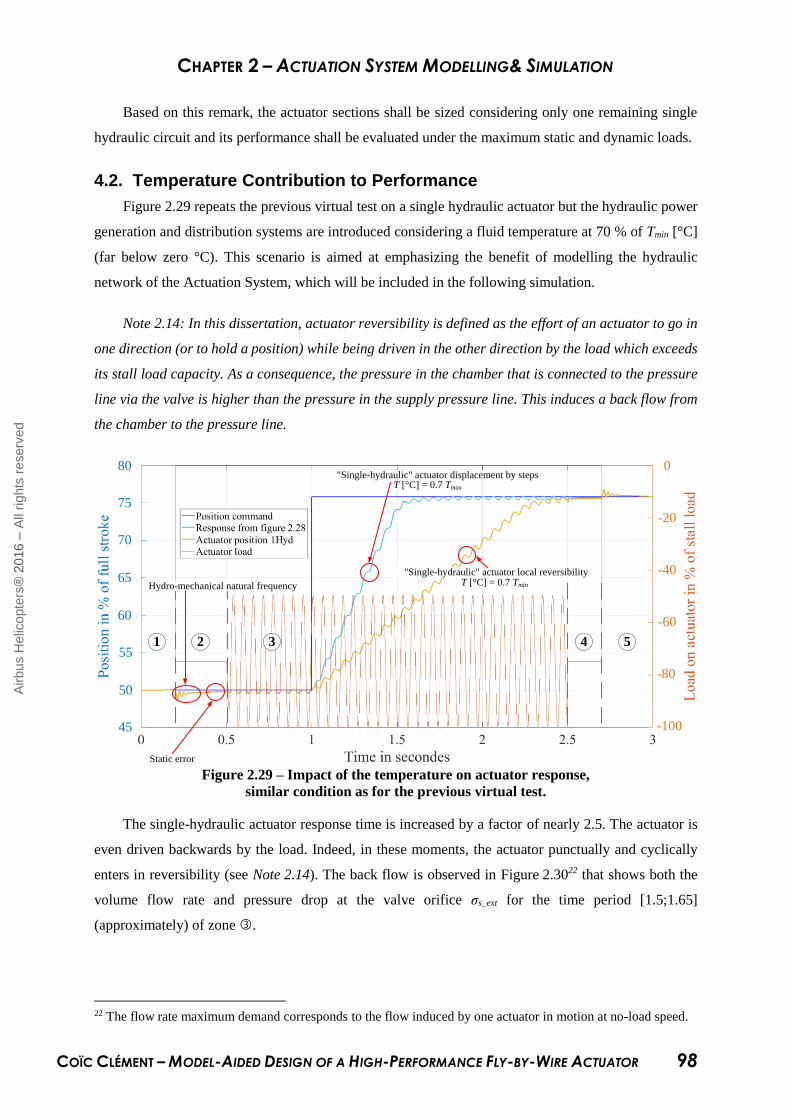
CHAPTER 2 – ACTUATION SYSTEM MODELLING& SIMULATION
COÏC CLÉMENT – MODEL-AIDED DESIGN OF A HIGH-PERFORMANCE FLY-BY-WIRE ACTUATOR 98
Based on this remark, the actuator sections shall be sized considering only one remaining single
hydraulic circuit and its performance shall be evaluated under the maximum static and dynamic loads.
4.2. Temperature Contribution to Performance
Figure 2.29 repeats the previous virtual test on a single hydraulic actuator but the hydraulic power
generation and distribution systems are introduced considering a fluid temperature at 70 % of Tmin [°C]
(far below zero °C). This scenario is aimed at emphasizing the benefit of modelling the hydraulic
network of the Actuation System, which will be included in the following simulation.
Note 2.14: In this dissertation, actuator reversibility is defined as the effort of an actuator to go in
one direction (or to hold a position) while being driven in the other direction by the load which exceeds
its stall load capacity. As a consequence, the pressure in the chamber that is connected to the pressure
line via the valve is higher than the pressure in the supply pressure line. This induces a back flow from
the chamber to the pressure line.
1 2 3 4 5
Hydro-mechanical natural frequency
Static error
T [°C] = 0.7 Tmin
T [°C] = 0.7 Tmax
"Single-hydraulic" actuator displacement by steps
"Single-hydraulic" actuator local reversibility
80
75
70
65
60
55
50
45
0
-20
-40
-60
-80
-100
Figure 2.29 – Impact of the temperature on actuator response,
similar condition as for the previous virtual test.
The single-hydraulic actuator response time is increased by a factor of nearly 2.5. The actuator is
even driven backwards by the load. Indeed, in these moments, the actuator punctually and cyclically
enters in reversibility (see Note 2.14). The back flow is observed in Figure 2.3022 that shows both the
volume flow rate and pressure drop at the valve orifice σs_ext for the time period [1.5;1.65]
(approximately) of zone .
22 The flow rate maximum demand corresponds to the flow induced by one actuator in motion at no-load speed.
Airb
us H
elic
opte
rs®
2016 –
All
rights
reserv
ed

CHAPTER 2 – ACTUATION SYSTEM MODELLING& SIMULATION
COÏC CLÉMENT – MODEL-AIDED DESIGN OF A HIGH-PERFORMANCE FLY-BY-WIRE ACTUATOR 99
Local reversibilities
35
Pressure drop at valve orifice σs_ext in % of the half of the supply pressure
Volume flow rate required at valve orifice σs_ext in % of the maximum demand
30
25
20
15
10
5
0
-5
Zoom zone 3
Figure 2.30 – Pressure-difference available at actuator inlet
and volume flow rate required in the pressure line.
As the loading is identical to the previous test, the reversibility is due to the pressure losses in the
supply and return pipes, which reduce the pressure available at the actuator inlet/outlet. This virtually
decreases the actuator stall load capability.
This effect is even more perceptible when the position error (the difference between the input
command and the actuator position) corresponds to the maximal opening of the valve. The fluid is no
longer kept in the cylinder when the load induces higher chamber pressures than the one available at the
actuator inlet/outlet.
Note 2.15: Recalling Equation 2.9, flow section σ is maximal and the pressure drop at the valve
orifice ΔP is negative. Thus, the flow is negative; it goes out of the cylinder.
2( )qQ c P sign P
Reminder of Equation 2.9
Based on these observations and in addition to the previous recommendation, the sizing point shall
be assessed considering the minimum operating fluid temperature.
4.3. Actuator Couplings
This last section emphasizes the need for simulating the entire Actuation System. The difference to
the previous section is that the four actuators (three main rotor and one tail rotor actuators) are modelled.
Airb
us H
elic
opte
rs®
2016 –
All
rights
reserv
ed

CHAPTER 2 – ACTUATION SYSTEM MODELLING& SIMULATION
COÏC CLÉMENT – MODEL-AIDED DESIGN OF A HIGH-PERFORMANCE FLY-BY-WIRE ACTUATOR 100
Indeed, a coupling between the actuators exists and is illustrated in Figure 2.31. It shows that the
performance of one actuator can depend on the other actuators' commands and responses.
As an example, the following test case has been simulated. On one side, a single-hydraulic actuator
(the so-called “fore” actuator) faces its stall load but is required to hold a centred position – since zone
. On the other side, the three other actuators are not exposed to any load but their input command is a
ramp of 25 % of the full stroke per second – since zone . The induced flow demand corresponds to
30 % of the maximum pump capability. In this scenario, the fluid temperature remains at 70 % of Tmin
[°C].
After two seconds of initialisation (zone ), it is possible to observe that the pressure-difference
available at the fore actuator is near 98 % of the supply pressure. The reduction of 2 % of the supply
pressure is induced by the four actuator valve leakages.
Since zone , the fore actuator enters in reversibility due to the pressure drop induced by the other
actuator motions that require a volume flow rate. Thus, the pressure drop specified for one actuator
design shall consider the potential motions of the other actuators.
1 2 3 4
T [°C] = 0.7 Tmax
"Single-hydraulic" actuator reversibility
30
20
10
0
-10
-20
-30
100
90
80
70
60
70
60
Figure 2.31 – Actuator response couplings.
It is interesting to note that actuator sinking is progressive for nearly 0.6 seconds. This can be
explained as, in zone , the valve is almost closed23. The supply pressure decreases due to the other
actuators motion, therefore the fore actuator enters in reversibility. But, the valve being almost closed,
it creates a high restriction for the flow to get out of the cylinder. Thus the sinking is slow. However,
23 Indeed, this small opening is induced by the load (and the closed loop gain), which causes a static error
necessary to open the valve enough to provide the required pressure.
Airb
us H
elic
opte
rs®
2016 –
All
rights
reserv
ed

CHAPTER 2 – ACTUATION SYSTEM MODELLING& SIMULATION
COÏC CLÉMENT – MODEL-AIDED DESIGN OF A HIGH-PERFORMANCE FLY-BY-WIRE ACTUATOR 101
while the position error increases, the valve opening also does and thus creates less and less restriction,
allowing a higher negative speed to the piston-cylinder assembly (zone ). Once the valve reaches its
maximal opening (zone ), an equilibrium is found and the sinking continues at a constant speed.
1 2 3 4
80
60
40
0
25
20
100
20
15
10
5
0
-5
-10
-15
-20
-25
Sinking actuator provides flow to the other one.
Figure 2.32 – Actuator response couplings: communicating flow rates.
Figure 2.32 shows an interesting aspect of the actuator couplings. The sinking of the fore actuator
provides a volume flow rate to the hydraulic power distribution which benefits the other actuators.
Therefore, a lower volume flow rate is required from the pump in zone .
Note 2.16: This illustrates once again the need for simulating the entire actuation system. However,
no recommendations should be extracted from this observation as the actuator sinking is not desirable
and shall never occur in the entire helicopter flight domain.
4.4. Actuation System Simulation
As a premise to these “coupled” simulations, it should be pointed out that each component involved
in the Actuation System model has been verified unitarily, based on tests of the physical prototypes
performed on test benches.
Integration tests of the Actuation System modelling have been done re-playing real command and
load scenarios considering flight recordings.
Finally, this modelling has been integrated in a global flight control system model which involves
the helicopter dynamics, realistic flight loads, the autopilot commands, etc. It enabled evaluating several
architectures of a new Actuation System and verifying its final design at helicopter level [COI16c].
Airb
us H
elic
opte
rs®
2016 –
All
rights
reserv
ed
CHAPTER 2 – ACTUATION SYSTEM MODELLING& SIMULATION
COÏC CLÉMENT – MODEL-AIDED DESIGN OF A HIGH-PERFORMANCE FLY-BY-WIRE ACTUATOR 102
5. CONCLUSION
Virtual models are widely used within the product lifecycle management from the early
development phase on. They enable reducing the development time while ensuring a better fulfilment
of the entire specification before the physical model is available. However, virtual models are also a
potential source of error.
Therefore, in the first section, after introducing the terminology required for understanding, the
modelling and simulation errors were detailed and illustrated with examples. It was concluded stating
that effort must be put in architecting the models in order to reduce the number of errors.
The model architecting is addressed based on engineering and industrial needs. The Bond-graph
formalism perfectly fits these needs and is therefore selected for the virtual model development. New
concepts were proposed to improve model readability, balancing and readiness for further uses. Ways
to model each physical domain involved in the Actuation System were detailed. Standardization of
mechanical components was presented and widely used, thus highlighting their genericity. Standardized
mechanical components are object-oriented and facilitate the creation of new mechanical virtual models
while reducing the number of possible errors in the modelling phase.
Each subsystem of the Actuation System virtual model was detailed, component by component.
An effort was made to standardize the interfaces using causal bonds, so that each subsystem from the
same domain can easily be connected. This ensures correctness of further implementation in simulation
software.
Finally, it was decided to simulate specific scenarios to illustrate how this modelling capitalizes
knowledge and enables new studies to be carried out almost effortlessly. In this particular case, actuator
sizing recommendations were provided regarding loads, temperature and Actuation System couplings.
These simulations reinforce the need to implement a global Actuation System virtual model to evaluate
new architectures of designs.
This complete virtual model has been used with success for a new helicopter development. Its aim
is to size the actuators correctly, not only based on a sub-system specification (the actuator specification)
but also based on a simulation verifying compliance with the Actuation System specification, in order
to avoid oversizing or, even worse, undersizing of the actuators.
Airb
us H
elic
opte
rs®
2016 –
All
rights
reserv
ed
CHAPTER 2 – ACTUATION SYSTEM MODELLING& SIMULATION
COÏC CLÉMENT – MODEL-AIDED DESIGN OF A HIGH-PERFORMANCE FLY-BY-WIRE ACTUATOR 103
BIBLIOGRAPHY
[ASH56] ASHBY, W.R., An Introduction to Cybernetics, John Wiley, New York, 1956.
[ATT08] ATTAR, B., Modélisation Réaliste en Conditions Extrêmes des Servovalves
Électrohydrauliques Utilisées pour le Guidage et la Navigation Aéronautique et
Spatiale. Toulouse, France, 2008. (in French)
[BAR93] BARUS, C., Isothermals, isopiestics and isometrics relative to viscosity. American
Journal of Science, pp87-96, 1893.
[BEA88] BEAMAN, J.J. & ROSENBERG, R.C., Constitutive and Modulation Structure in Bond
Graph Modeling. Journal of Dynamic Systems, Measurement and Control, pp.395-402,
1988.
[BOE95] BOES, C., Hydraulische Achsantriebe im digitalen Regelkreis. RWTH Aachen, 1995.
(in German)
[BOR10] BORUTZKY, W., Bond Graph Methodology: Development and Analysis of
Multidisciplinary Dynamic System Models. New York: Springer-Verlag, 2010.
[BOR11] BORUTZKY, W., Bond Graph Modelling of Engineering Systems – Theory, Applications
and Software Support. New York: Springer-Verlag, 2011.
[BRE82] BREEDVELD, P.C., The Thermodynamic Bond Graph Concept Applied to a Flapper
Nozzle Valve. Proceedings of the 10th IMACS World Congress on Systems Simulation
and Scientific Computation, volume 3, pp 395-397, 1982.
[BRE13] BREEDVELD, P.C., Integrated Modeling of Physical Systems, Dynamic Systems part III.
Lecture notes, University of Twente, 2013.
[CEL91] CELLIER, F.E., Continuous System Modelling. Springer Science, 1991.
[CEL13] CELLIER, F.E., Improvements in BondLib, the Modelica Bond Graph Library. Proc. of
the 2013 8th EUROSIM Congress on Modelling and Simulation, 2013.
[CLO80] MC CLOY, D. & MARTIN, H.R., Control of Fluid Power – Analysis and design. John
Wiley & Sons, New York, 1968.
[COI16a] COÏC, C. & MARÉ, J.-C., Modeling and Pre-Sizing Process for Hydrostatic Thrust
Bearing with Special Consideration to Performance Robustness within a Wide
Temperature Range, International Conference on Hydraulics and Pneumatics, Praha,
Czech Republic, 2016.
[COI16b] COÏC, C., FU, J. & MARÉ, J.-C., Bond Graphs Aided development of Mechanical Power
Transmission for Aerospace Electromechanical Actuators, International Conference on
Bond Graph Modelling, Montréal, Canada, 2016.
[COI16c] COÏC, C., BYZERY, R., MARGER, T. & ALLIETTA, J.-M., Optimization of the Actuation
System Sizing of a new Helicopter based on Global Modeling Approach, Recent
Advances in Aerospace Actuation Systems and Components, Toulouse, France, 2016.
[DAU00] DAUPHIN-TANGUY, G., Les bonds graphs, HERMES Science, Paris, 2000. (in French)
[EGG80] EGGERTH, S., Beitrag zur Messung von Volumenströmen viskoser Flüssigkeiten in
Druckleitungen. Technische Universität Dresden, 1980. (in German)
Airb
us H
elic
opte
rs®
2016 –
All
rights
reserv
ed

CHAPTER 2 – ACTUATION SYSTEM MODELLING& SIMULATION
COÏC CLÉMENT – MODEL-AIDED DESIGN OF A HIGH-PERFORMANCE FLY-BY-WIRE ACTUATOR 104
[EIG12] EIGNER, M., GILZ, T. & ZAFIROV, R., Proposal for functional product description as
part of a PLM solution in interdisciplinary product development. In International
Design Conference, Dubrovnik, 2012.
[EUR04] EUROCOPTER, AS332 Instruction Manual. Marignane, 2004.
[FAI83] FAISANDIER, J., Mécanismes hydrauliques. Dunod, Paris, 1983. (in French)
[FU15] FU, J., MARÉ, J.-C., FU, Y. & HAN, X., Incremental Modelling and Simulation of Power
Drive Electronics and Motor for Flight Control Electro-Mechanical Actuators
Application. Proceedings of 2015 IEEE, International Conference on Mechatronics and
Automation, Beijing, China, 2015.
[GAI79] GAINES, B., "General Systems Research: Quo Vadis," General Systems Yearbook, pp.
1-9 1979.
[GIL92] GILLE, J.-C., DECAULNE, P. & PELEGRIN, M., Théorie et Calcul des Asservissements
Linéaires, Dunod, Paris, 1992. (in French)
[GUI92] GUILLON, M., Commande et asservissement hydrauliques et électrohydrauliques.
Lavoisier, Paris, 1992. (in French)
[HOF81] HOFFMANN, W., Dynamisches Verhalten hydraulischer Systeme, automatischer
Modellaufbau und digitale Simulation. RWTH Aachen, 1981. (in German)
[IDE66] IDEL’CHICK, I.E., Handbook of hydraulic resistance. Israël Program for Scientific
Translations, 1966.
[JIN94] JINGHONG, Y., ZHAONENG, C. & YUANZHANG, L., The Variation of Oil Effective Bulk
Modulus With Pressure in Hydraulic Systems. Transaction of the ASME. Journal of
Dynamic Systems, Measurement and Control, pp116-144, 1994.
[KAR06] KARAM, W. & MARÉ, J.-C., Comparison of EMA and HA performance for dynamic
load simulators. Proc. Bath Power Transmission and Motion Control Symposium –
PTMC 2006, pp211-224, 2006.
[KAR12] KARNOPP, D.C., MARGOLIS, D.L., & ROSENBERG, R.C., System dynamics: modelling,
simulation, and control of mechatronic systems. 5th ed. New York: John Wiley & Sons,
2012.
[KOR78] KORN, G.A. & WAIT, J.V., Digital Continuous System Simulation, Prentice-Hall,
Englewood Cliffs, N.J., 1978.
[LEB84] LEBRUN, M., Normal Modes in Hydraulic Lines. American Control Conference,
pp.458-467, San Diego, USA, 1984.
[LEE77] LEE, K.I., Dynamisches Verhalten der Steuerkette Servoventil - Motor- Last. RWTH
Aachen, 1977. (in German)
[LIN14] VAN DER LINDEN, F.L.J., General Fault Triggering Architecture to Trigger Model
Faults in Modelica using a Standardized Blockset, Proceedings of the 10th International
Modelica Conference, Lund, 2014.
[MAR93] MARE, J.-C. Contribution à la modélisation, la simulation, l’indentification et la
commande d’actionneurs électrohydrauliques. Thèse d’état, Lyon, 1993. (in French)
Airb
us H
elic
opte
rs®
2016 –
All
rights
reserv
ed

CHAPTER 2 – ACTUATION SYSTEM MODELLING& SIMULATION
COÏC CLÉMENT – MODEL-AIDED DESIGN OF A HIGH-PERFORMANCE FLY-BY-WIRE ACTUATOR 105
[MAR00] MARE, J.-C., Commande numérique - bien spécifier pour maîtriser les effets parasites,
Revue Fluides, pp 41-45, N°17, 2000. (in french)
[MAR01] MARÉ, J.-C., Simplified model of pressure regulated, variable displacement pumps for
the sizing of complex hydraulic systems, Proceedings of the 5th International Conference
on fluid Power transmission and Control, Hangzhou, pp151-155, April 3-5, 2001.
[MAR12] MARÉ, J.-C., 2-D lumped paramaters modelling of EMAs for advanced virtual
prototyping. Proc. International Conference on Recent Advances in Aerospace
Actuation Systems and Components (R3ASC), p. 122-127, Toulouse, 2012.
[MAR16] MARÉ, J.-C., Requirement-based system-level simulation of mechanical transmissions
with special consideration of friction, backlash and preload, SIMPAT1572, Simulation
Modelling Practice and Theory, p58-82, 2016.
[MARG11] MARGER, T., Valve Design of Hydro-Mechanical Servoactuator under Cost and
Mixability Criteria. Arts et Métiers ParisTech, 2011.
[MARQ11] MARQUIS-FAVRE, W. & JARDIN, A., Bond Graph pour la Conception de Systèmes
Mécatroniques. Techniques de l’Ingénieur D 3065, 2011.
[MER67] MERRITT, H.E., Hydraulic Control System, John Wiley & sons, Inc., 1967.
[MIN65] MINSKY, M., Models, Minds, Machines, Proceedings IFIP Congress, pp. 45-49, 1965.
[MOO14] MOOG, Type 30, Nozzle-Flapper Flow Control Servovalves. East Aurora, 2014.
[MUV10] MUVENGEI, O. & KIHIU, J., Bond Graph Modelling of Inter-actuator Interactions in a
Multi-cylinder Hydraulic System, International Journal of Mechanical, Industrial and
Aerospace Engineering, Vol.4 (1), 2010.
[NIK33] NIKURADSE, J., Strömungsgesetze in rauhen Rohren, VDI-Forschungsheft 361, 1933.
(in German)
[OUL06] OULD BOUAMAMA, B. and DAUPHIN-TANGUY, G., Modélisation par bond graph,
Application aux systèmes énergétiques, Techniques de l’Ingénieur BE 8 281, 2006.
(in French)
[PAY61] PAYNTER, H.M., Analysis and Design of Engineering Systems, The M.I.T. Press, 1961.
[PRŠ13] PRŠIĆ, D., NEDIĆ, N. & DUBONJIĆ, L., Modeling and Simulation of Hydraulic Long
Trasmission Line by Bond Graph, Journal of Mechanics Engineering and Automation
3, pp.257-262, 2013.
[PRU70] PRUDHOMME, R., Automatique – Tome 1, Systèmes Séquentiels à Niveau ; Systèmes
Asservis Linéaires Continus, Masson & CIE, Paris, 1970. (in French)
[RAB81] RABIE, G. & LEBRUN, M., Modélisation par les Graphes à Liens et Simulation d’une
Servovalve à deux Étages, R.A.I.O. Automatique/Systems Analysis and Control, 15,
pp.97-129, 1981.
[REC00] RECHTIN, E., The Art of Systems Architecting, CRC Press LLC, 2000.
[REY86] REYNOLDS, 0., On the Theory of Lubrication and its Application to Mr. Beauchamp
Tower’s Experiments, including an Experimental Determination of the Viscosity of
Olive Oil, 1886.
[ROM00] ROMAN, C., Flow Control Servovalve Model, Imagine, Roanne, 2000.
Airb
us H
elic
opte
rs®
2016 –
All
rights
reserv
ed

CHAPTER 2 – ACTUATION SYSTEM MODELLING& SIMULATION
COÏC CLÉMENT – MODEL-AIDED DESIGN OF A HIGH-PERFORMANCE FLY-BY-WIRE ACTUATOR 106
[SAE00] S.A.E., AIR 1362 – Aerospace Hydraulic Fluids Physical Properties. USA, 2000.
[SAE12] S.A.E., ARP 994 – Recommended Practice for the Design of Tubing Installations for
Aerospace Fluid Power Systems. USA, 2012.
[SOM06] SOMASHEKHAR, S.H., SINGAPERUMAL, M. & KUMAR, R.K., Modelling the Steady-State
Analysis of a Jet Pipe Electrohydraulic Servo Valve. Proceedings of the Institution of
Mechanical Engineers, Part I, Journal of System and Control Engineering, vol. 220,
pp.109,130, 2006.
[SJÖ10] SJÖLUND, M., BRAUN, R., FRITZSON, P. & KRUS, P., Towards Efficient Distributed
Simulation in Modelica Using Transmission Line Modeling. 3rd International Workshop
on Equation-Based Object-Oriented Languages and Tools, Norway, 2010.
[TCH79] TCHOUPRAKOV, Y., Commande Hydraulique et Automatismes Hydrauliques, Ed MIR,
Moscow, 1979.
[THO75] THOMA, J.U., Introduction to Bond Graphs and their applications, Pergamon Press,
1975.
[THO90] THOMA, J.U., Simulation by Bondgraphs - Introduction to Bond Graphs and their
applications, Springler-Verlag, 1990.
[THO99] THOMA, J.U. & HALIN, H.J., Bondgraphs and Practical Simulation, Simulation Practice
and Theory 7, pp.401-417, Elsevier, 1999.
[VDI04] VDI GUIDELINE 2206, Entwicklungsmethodik für mechatronische Systeme – Design
methodology for mechatronic systems, Beuth, 2004. (in German)
[VEL03] VELAZQUEZ, G. & MARÉ, J.-C., Bottom-up design of a variable displacement vane
pumps for automotive gearbox, Proceedings of the 8th Scandinavian International
Conference on Fluid Power, Tampere, Finland, 2003.
[XU13] XU, Y., Modelling and Control of a High Performance Electro-Hydraulic Test Bench,
INSA de Lyon, 2013.
[ZEI76] ZEIGLER, B.P., Theory of Modelling and Simulation, John Wiley, New York, 1976.
Websites:
[web20Sim] www.20sim.com, accessed on 20/07/2016.
[webAME] www.plm.automation.siemens.com/en_us/products/lms/imagine-lab/amesim/,
accessed on 20/07/2016.
[webBAR] http://www.barnesballscrew.com/how-a-ball-screw-works/ accessed on 02/09/2016
[webDYM] www.3ds.com/products-services/catia/products/dymola, accessed on 20/07/2016.
[webMAT] www.mathworks.com/products/matlab/, accessed on 20/07/2016.
Airb
us H
elic
opte
rs®
2016 –
All
rights
reserv
ed

COÏC CLÉMENT – MODEL-AIDED DESIGN OF A HIGH-PERFORMANCE FLY-BY-WIRE ACTUATOR 107
CHAPITRE 3
METHODES DE DIMENSIONNEMENT DE PALIERS FLUIDES LINEAIRES
SOUS CONTRAINTES AERONAUTIQUES
L’introduction de cette dissertation adressait les limitations actuelles des technologies de joints
dynamiques et des moyens de guidages. Les paliers fluides linéaires ont été identifiés comme une
alternative intéressantes pour le guidage en translation de l’ensemble piston-tige, en générant un effort
de recentrage, au coût d’une faible fuite de fluide entre les chambres. Les paliers fluides pourraient être
la clé de l’augmentation des performances des actionneurs sans dégrader excessivement sa durée de vie.
Le terme palier fluide inclus les paliers hydrostatiques, hydrodynamiques et hybrides. Comme leurs
noms l’indiquent, les deux premiers types de paliers fluides listés utilisent respectivement :
Les forces hydrostatiques, générée par la pression sur une surface « fixe ».
Les effets hydrodynamiques du fluide, créés par la variation de pression induite par un déplacement
relatif de deux surfaces.
Un palier fluide est qualifié d’hybride lorsqu’il combine les deux effets susnommés. Appliqués aux
cas des actionneurs hydrauliques, le mouvement relatif entre l’ensemble piston-tige et le corps du vérin
génère un effet hydrodynamique. Aussi, la pression dans les chambres du vérin induit un effort
hydrostatique. Ainsi, seuls les paliers hybrides sont candidats à la substitution des fonctions de guidages
dans vérins.
Néanmoins, dans le cas d’un paliers fluide hybride, le principe de superposition s’applique
pleinement, révélant ainsi l’intérêt d’étudier séparément les paliers hydrostatiques et hydrodynamiques.
Pour l’ensemble de ce chapitre, trois critères de dimensionnement des paliers sont mis en avant : la
génération d’effort normal ou de recentrage du palier fluide, son débit induit et la raideur normale ou
radiale associée. Le dernier critère rend compte de la volonté de générer un effort de recentrage croissant
avec l’augmentation de l’excentricité de l’ensemble piston-tige dans le corps du vérin. La complexité
de satisfaire ces trois critères dans une application aéronautique réside grandement dans le domaine
étendu de variation de température du fluide hydraulique ().
La première partie de ce chapitre porte sur l’étude d’un filet de fluide générique. Cette section 1 a
pour but de présenter les équations prise en compte dans ce type d’étude. Une attention particulière est
Airb
us H
elic
opte
rs®
2016 –
All
rights
reserv
ed

CHAPITRE 3 – METHODES DE DIMENSIONNEMENT DE PALIERS FLUIDES LINEAIRES
COÏC CLÉMENT – MODEL-AIDED DESIGN OF A HIGH-PERFORMANCE FLY-BY-WIRE ACTUATOR 108
portée sur la non-simplification des équations de manière à mettre en évidence tous les effets permettant
de générer des variations de pression dans le filet de fluide. Le résultat est l’équation de Reynolds
(Equation 3.6). Chaque terme de cette équation est discuté ainsi que leur intérêt dans notre étude.
Dans la section 2, trois différents designs de surface sont étudiés : plans parallèles, plans inclinés
et plan en escalier. Les équations modélisant leurs capacités respectives à générer un effort normal, leurs
débits de fuite induit ainsi que leurs raideurs sont analytiquement déterminées. Table 3.1 regroupe les
équations des trois critères d’intérêt pour les trois surfaces étudiées. Deux des trois surfaces sont
sélectionnées pour la suite de notre étude. En effet, la solution impliquant des plans parallèles ne génère
aucune raideur radiale ce qui est rédhibitoire pour notre application.
La section 3 a fait l’objet d’une communication présentée en Keynote lors de la conférence
internationale sur l’hydraulique et pneumatique à Prague en 2016 [COI16a]. Cette section détaille la
modélisation et un processus pré-dimensionnement des paliers fluides hydrostatiques sous contraintes
aéronautiques. Ces contraintes induisent une attention particulière à la robustesse des performances dans
l’ensemble du domaine étendu de variation de température du fluide. Afin de satisfaire l’ensemble de
nos critères, un orifice tube-court (« short tube orifice » en anglais) est inséré en tant que restriction
amont nécessaire à la raideur du palier. Ce type d’orifice introduit un paramètre de dimensionnement
d’intérêt, lequel peut aisément être adapté de manière à répondre au dilemme force/raideur versus débit
de fuite sur la plage de variation de température du fluide.
Finalement, dans la section 4, une étude de sensibilité est menée sur les paliers hybrides coniques.
Elle adresse la variation des trois principaux critères de dimensionnement face aux variables temporelles
(i.e. température et excentration), ainsi que face aux paramètres de dimensionnement (i.e. la forme du
palier). Les dangers liés à un mauvais design de paliers fluides, sur l’ensemble de la plage de température
opérationnelle, sont mis en évidence. Notamment, cela peut conduire à un effort de recentrage négatif
(soit excentrant l’ensemble piston-tige dans le corps du vérin) aux faibles températures. En effet, aux
basses températures, l’effort hydrodynamique induit par le mouvement relatif des surfaces du palier peut
annuler et même surpasser l’effort hydrostatique, généré par la pression dans les chambres du vérin. Des
recommandations concernant le dimensionnement géométrique du palier sont finalement adressées de
manière à satisfaire aux mieux les critères d’effort normal, de débit de fuite induit et de raideur du palier,
pour l’ensemble de la plage de température.
Airb
us H
elic
opte
rs®
2016 –
All
rights
reserv
ed
COÏC CLÉMENT – MODEL-AIDED DESIGN OF A HIGH-PERFORMANCE FLY-BY-WIRE ACTUATOR 109
CHAPTER 3:
METHODS OF LINEAR FLUID BEARING DESIGN
UNDER AEROSPACE CONSTRAINTS
The Introduction of this dissertation addressed the limits of current dynamic sealing and bearing
devices. Linear fluid bearings were identified as an interesting alternative for guiding the piston-rod in
translation and resisting to radial forces, at the cost of minor leakage. Fluid bearings would increase
actuator performance without excessively reducing its lifespan. Their main function is to guide the
piston-rod assembly while allowing for a relative movement between both components without
mechanical contact.
The term fluid bearing includes hydrostatic, hydrodynamic and hybrid bearings. As their names
indicate, hydrostatic and hydrodynamic bearings respectively make use of:
the hydrostatic force of the fluid, generated by an existing pressure on a “fixed” surface.
the hydrodynamic effect24 of the fluid, created by a pressure variation induced by a relative motion
between surfaces.
A fluid bearing is called hybrid when it combines both hydrostatic and hydrodynamic effects. In
our application, on the one hand, the relative motion between the piston-rod assembly and the actuator
housing generates a hydrodynamic effect. On the other hand, the pressure chambers create a hydrostatic
effect. Therefore, purely hydrodynamic or hydrostatic bearings cannot be used in our case, but hybrid
bearings can.
In order to support the analysis of the different fluid bearings, the general case of a fluid film is
studied in section 1. The aim is to introduce the equations that are used later in this chapter.
Section 2 presents the different surface designs leading to the generation of a normal force by the
fluid film. As a first approach, lateral flow is neglected in order to render the functioning of each solution
easily understandable. Two of the three designs presented are selected for a more thorough study under
aerospace constraints in the next sections.
Section 3 details a modelling and pre-sizing process for hydrostatic thrust bearings with special
attention being paid to performance robustness within a wide temperature range. Thrust bearings are
studied here as combining at least three of them located at different azimuths is equivalent to a
24 It is here preferred to use the term effect rather than force as hydrodynamic force is more generally used to
describe the change in fluid momentum. [MAR93]
Airb
us H
elic
opte
rs®
2016 –
All
rights
reserv
ed
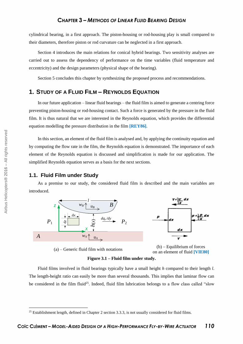
CHAPTER 3 – METHODS OF LINEAR FLUID BEARING DESIGN
COÏC CLÉMENT – MODEL-AIDED DESIGN OF A HIGH-PERFORMANCE FLY-BY-WIRE ACTUATOR 110
cylindrical bearing, in a first approach. The piston-housing or rod-housing play is small compared to
their diameters, therefore piston or rod curvature can be neglected in a first approach.
Section 4 introduces the main relations for conical hybrid bearings. Two sensitivity analyses are
carried out to assess the dependency of performance on the time variables (fluid temperature and
eccentricity) and the design parameters (physical shape of the bearing).
Section 5 concludes this chapter by synthesizing the proposed process and recommendations.
1. STUDY OF A FLUID FILM – REYNOLDS EQUATION
In our future application – linear fluid bearings – the fluid film is aimed to generate a centring force
preventing piston-housing or rod-housing contact. Such a force is generated by the pressure in the fluid
film. It is thus natural that we are interested in the Reynolds equation, which provides the differential
equation modelling the pressure distribution in the film [REY86].
In this section, an element of the fluid film is analysed and, by applying the continuity equation and
by computing the flow rate in the film, the Reynolds equation is demonstrated. The importance of each
element of the Reynolds equation is discussed and simplification is made for our application. The
simplified Reynolds equation serves as a basis for the next sections.
1.1. Fluid Film under Study
As a premise to our study, the considered fluid film is described and the main variables are
introduced.
P1
x
z
h(x
)
dz
dx
P2
uBwB
uAwAA
Bl l
dqx /dy
(a) – Generic fluid film with notations (b) – Equilibrium of forces
on an element of fluid [VIE80]
Figure 3.1 – Fluid film under study.
Fluid films involved in fluid bearings typically have a small height h compared to their length l.
The length-height ratio can easily be more than several thousands. This implies that laminar flow can
be considered in the film fluid25. Indeed, fluid film lubrication belongs to a flow class called “slow
25 Establishment length, defined in Chapter 2 section 3.3.3, is not usually considered for fluid films.
Airb
us H
elic
opte
rs®
2016 –
All
rights
reserv
ed

CHAPTER 3 – METHODS OF LINEAR FLUID BEARING DESIGN
COÏC CLÉMENT – MODEL-AIDED DESIGN OF A HIGH-PERFORMANCE FLY-BY-WIRE ACTUATOR 111
viscous motion” [HAM04] where inertia effects can be neglected. This assertion is valid for the entire
chapter and is verified after each pre-sizing in order to emphasize its correctness.
Figure 3.1-(a) represents the fluid film considered in our study. The film is delimited by two
surfaces A and B in motion at speeds u and w (with subscript A and B) regarding respectively the x and
z axes. A is considered to be extremely long with respect to B so the fluid film always exists. In addition,
A is considered to be a plane surface so that the reference frame can be easily located; the shape defects
are projected on B. The height of the fluid film can vary over the film length. For reasons of readability,
in this figure, the length-height ratio is not representative of the order of magnitude previously described.
As a simplification for our study, the conditions are considered identical along the y axis. It is
therefore only necessary to focus on an infinitely small slice in the y direction. Thus, the variable dqx/dy
is the surface flow rate26 in the fluid film.
1.2. Continuity Equation
The continuity equation ensures the balance of mass in a volume. The difference between the output
and input flows of mass from a volume of fluid must be equal to the variation of mass within the volume.
Considering an element of fluid volume dV = dx dy dz, the continuity equation can be written as follows:
u v w dxdy dz dxdy dzx y z t
Equation 3.1
where:
t is the time [s]
v is the surface speed along the y axis [m/s]
As detailed above, there is no variation along the y axis. Thus, after this simplification, it is possible
to integrate the continuity equation in order to study a surface element dS = h dx.
0
0h
u w dzt x z
Equation 3.2
This integral can be solved using Leibniz’s integral rule for the second term, leading to:
00
h
B A B
hh udz w w u
t x x
Equation 3.3
The next step, described in section 1.3, is thus to compute the remaining integral, which
corresponds to the surface flow rate dqx/dy. Each term of updated Equation 3.3 is then commented in
section 1.4.
26 The term “surface” is used in contrast to “volume” when the three dimensions are considered.
Airb
us H
elic
opte
rs®
2016 –
All
rights
reserv
ed
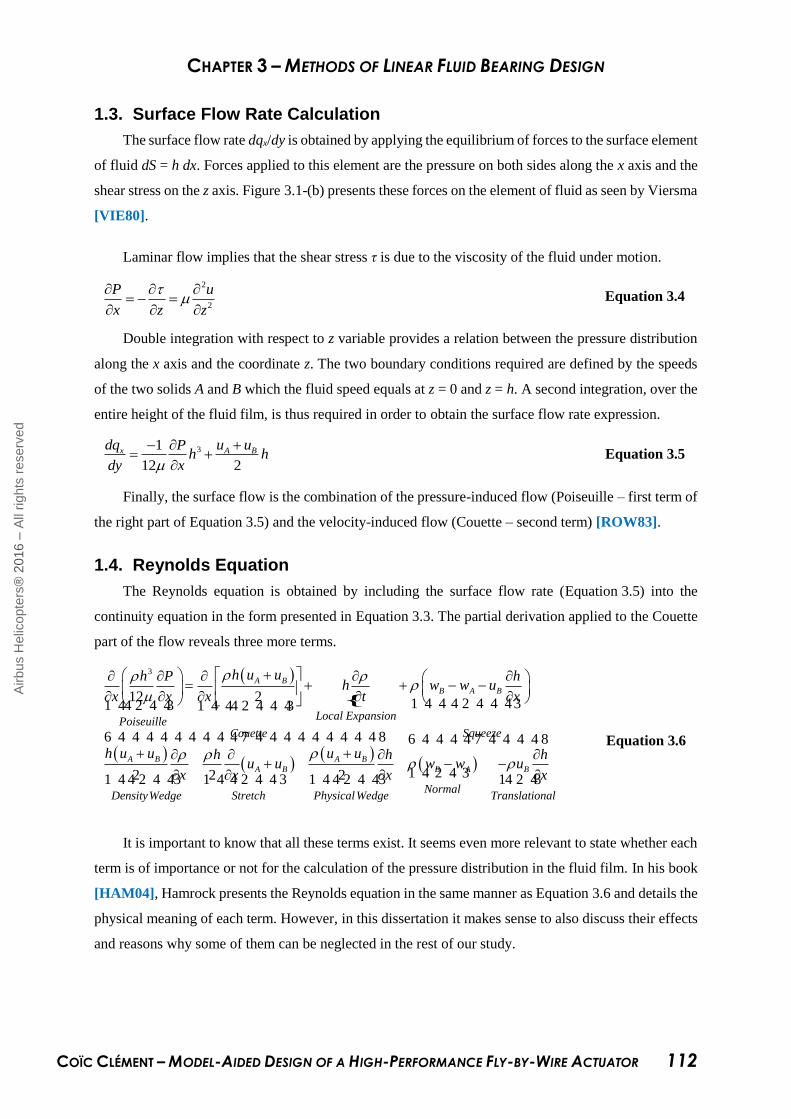
CHAPTER 3 – METHODS OF LINEAR FLUID BEARING DESIGN
COÏC CLÉMENT – MODEL-AIDED DESIGN OF A HIGH-PERFORMANCE FLY-BY-WIRE ACTUATOR 112
1.3. Surface Flow Rate Calculation
The surface flow rate dqx/dy is obtained by applying the equilibrium of forces to the surface element
of fluid dS = h dx. Forces applied to this element are the pressure on both sides along the x axis and the
shear stress on the z axis. Figure 3.1-(b) presents these forces on the element of fluid as seen by Viersma
[VIE80].
Laminar flow implies that the shear stress τ is due to the viscosity of the fluid under motion.
2
2
P u
x z z
Equation 3.4
Double integration with respect to z variable provides a relation between the pressure distribution
along the x axis and the coordinate z. The two boundary conditions required are defined by the speeds
of the two solids A and B which the fluid speed equals at z = 0 and z = h. A second integration, over the
entire height of the fluid film, is thus required in order to obtain the surface flow rate expression.
31
12 2
x A Bdq P u uh h
dy x
Equation 3.5
Finally, the surface flow is the combination of the pressure-induced flow (Poiseuille – first term of
the right part of Equation 3.5) and the velocity-induced flow (Couette – second term) [ROW83].
1.4. Reynolds Equation
The Reynolds equation is obtained by including the surface flow rate (Equation 3.5) into the
continuity equation in the form presented in Equation 3.3. The partial derivation applied to the Couette
part of the flow reveals three more terms.
{
3
12 2
2 2 2
A B
B A B
A B A B
A B
Local ExpansionPoiseuille
Co
DensityWedge Stretch PhysicalWedge
h u uh P hh w w u
x x x t x
h u u u uh hu u
x x x
1 4 4 4 2 4 4 431 44 2 4 43 1 4 44 2 4 4 43
1 4 4 2 4 43 1 4 4 2 4 4 3 1 4 4 2 4 43 B A B
Squeezeuette
NormalTranslational
hw w u
x
6 4 4 4 4 4 4 4 4 4 7 4 4 4 4 4 4 4 4 4 8 6 4 4 4 4 7 4 4 4 4 8
1 4 2 4 3 14 2 43
Equation 3.6
It is important to know that all these terms exist. It seems even more relevant to state whether each
term is of importance or not for the calculation of the pressure distribution in the fluid film. In his book
[HAM04], Hamrock presents the Reynolds equation in the same manner as Equation 3.6 and details the
physical meaning of each term. However, in this dissertation it makes sense to also discuss their effects
and reasons why some of them can be neglected in the rest of our study.
Airb
us H
elic
opte
rs®
2016 –
All
rights
reserv
ed
CHAPTER 3 – METHODS OF LINEAR FLUID BEARING DESIGN
COÏC CLÉMENT – MODEL-AIDED DESIGN OF A HIGH-PERFORMANCE FLY-BY-WIRE ACTUATOR 113
Stretch. The variation of speed along x axis of the surfaces A and B is not considered in this chapter
as the surfaces consist of rigid solids. (This does not mean that the speed of each surface does not
vary with time.)
Density wedge. Also referred to as thermal wedge [BLA60], it corresponds to the evolution of
density in the fluid film. Even if this effect cannot be neglected for parallel surfaces, Jacques
Faisandier demonstrates in [FAI83] the minor importance it has, compared to the physical wedge.
Also, it is important to recall that the experimental frame associated with the fluid model developed
in Chapter 2 only allows density variation if there is a change of pressure or temperature. The change
of pressure along the x axis could possibly be implemented, but it would require considering several
volumes in the film fluid, which is not desirable. Effort is made in the next sections to obtain a
virtual lumped parameter model for the bearings as the density wedge can be neglected. Regarding
the temperature variation along the x axis, this is outside the experimental frame. The fluid
temperature can only vary with time in our virtual models.
Physical wedge. The variation of the film height combined with surface motions generates a pressure
variation. Conical and step bearings make use of this effect by respectively causing a continuous or
discontinuous change of fluid film height. Therefore, it is widely used in this chapter. However, this
effect has to be combined with translational squeeze in order to perceive clearly the effect of the
surface speeds.
Translational squeeze. The motion of surface B forces the fluid to go through a section with a
different height, thus inducing pressure variation. The combination of translational squeeze and
physical wedge results in an expression that depends on the differential speed between the two
surfaces. This appears clearly in Equation 3.7. As a consequence, no pressure variation is induced
if no relative speed exists between surfaces A and B or if ∂h/∂x is zero.
Normal squeeze. This effect is the equivalent of translational speed in normal direction z. It is
important to note that no height variation with x is required. This effect is used for example in
dashpots, where the fluid film is the annular leakage and normal squeeze occurs in the dashpot
volume. Normal squeeze shall not be neglected. However, it is important to emphasize that radial27
motion is not relevant for our application: linear (axial) fluid bearings. Thus, this term often equals
zero, i.e. whenever equilibrium is reached in the radial position. On the contrary, translational
squeeze almost always operates as actuator motion is almost always required.
Local expansion. This term links the fluid density variation with time at a given position with the
induced pressure. Schmid [SCH14] affirms that this action is not important for fluid bearings.
27 In cylindrical applications, the fluid bearing normal force becomes a radial centring force.
Airb
us H
elic
opte
rs®
2016 –
All
rights
reserv
ed

CHAPTER 3 – METHODS OF LINEAR FLUID BEARING DESIGN
COÏC CLÉMENT – MODEL-AIDED DESIGN OF A HIGH-PERFORMANCE FLY-BY-WIRE ACTUATOR 114
Once all these effects have been described, in addition to the Poiseuille term, only the physical
wedge, the translational and normal squeezes are kept for further studying. This simplified Reynolds
equation is presented in Equation 3.7.
3
12 2
A B
B A
u uh P hw w
x x x
Equation 3.7
Finally, the density of the left part of the equation can be taken outside of the partial derivative.
The rationale is the same as for neglecting the density wedge. Thus, dividing Equation 3.7 by the fluid
density and rearranging the simplified Reynolds equation leads to:
3
12 2
A B
B A
u u hh Pw w
x x
Equation 3.8
This equation concludes this section. From the continuity equation, the Reynolds equation has been
obtained and the importance of each of its effects has been discussed. For surface analysis, Equation 3.8
includes the simplifications described and is used further below in this chapter as the basis of fluid
bearing applications.
2. CREATING A NORMAL FORCE IN FLUID BEARINGS
Fluid bearings allow a relative movement between two solids without mechanical contact. A
pressurized fluid film acts as interface between the two moving solids. The main criteria for the design
of fluid bearings are usually the normal force (to counterbalance an external load), the consumed flow
[ROW83] (main source of power dissipation) and the stiffness [POS89] (the ability to increase the
normal force with reduction of the film fluid height).
In continuity with section 1, axial analysis will be carried out based on Equation 3.8 in order to
determine the possible manners to obtain a normal force in fluid bearings. Associated consumed flow
and stiffness are discussed for each case.
Normal squeeze action is not considered. Position equilibrium on the z axis induces no relative
speed in this direction. Neglecting this effect is indeed conservative as it would dissipate energy.
2.1. Constant Height Fluid Film
2.1.1. Normal Force
A simple design could be a constant height fluid film. Once the normal squeeze action is neglected
and the height variation considered to be zero, Equation 3.8 becomes simply the double derivative of
the pressure with respect to x is zero. The pressure distribution along the fluid film is easily obtained
with a double integration. Boundary conditions are those of Figure 3.2-(b).
Airb
us H
elic
opte
rs®
2016 –
All
rights
reserv
ed
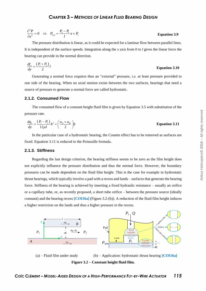
CHAPTER 3 – METHODS OF LINEAR FLUID BEARING DESIGN
COÏC CLÉMENT – MODEL-AIDED DESIGN OF A HIGH-PERFORMANCE FLY-BY-WIRE ACTUATOR 115
2
2 1( ) 12
0 x
P P PP x P
x l
Equation 3.9
The pressure distribution is linear, as it could be expected for a laminar flow between parallel lines.
It is independent of the surface speeds. Integration along the x axis from 0 to l gives the linear force the
bearing can provide in the normal direction.
1 2
2
xP Pdf
ldy
Equation 3.10
Generating a normal force requires thus an “external” pressure, i.e. at least pressure provided to
one side of the bearing. When no axial motion exists between the two surfaces, bearings that need a
source of pressure to generate a normal force are called hydrostatic.
2.1.2. Consumed Flow
The consumed flow of a constant height fluid film is given by Equation 3.5 with substitution of the
pressure rate.
31 2
12 2
x A BP Pdq u u
h hdy l
Equation 3.11
In the particular case of a hydrostatic bearing, the Couette effect has to be removed as surfaces are
fixed. Equation 3.11 is reduced to the Poiseuille formula.
2.1.3. Stiffness
Regarding the last design criterion, the bearing stiffness seems to be zero as the film height does
not explicitly influence the pressure distribution and thus the normal force. However, the boundary
pressures can be made dependent on the fluid film height. This is the case for example in hydrostatic
thrust bearings, which typically involve a pad with a recess and lands – surfaces that generate the bearing
force. Stiffness of the bearing is achieved by inserting a fixed hydraulic resistance – usually an orifice
or a capillary tube, or, as recently proposed, a short tube orifice – between the pressure source (ideally
constant) and the bearing recess [COI16a] (Figure 3.2-(b)). A reduction of the fluid film height induces
a higher restriction on the lands and thus a higher pressure in the recess.
dqx /dyP1
x
z
h P2
uB
uAA
B
l l
Recess
Pr
Short tube orifice
Orifice
Cap
illar
y tu
be
Ps Q
h
Variable
hydraulic
restriction
Lands
Patm
PadFixed
hydraulic
restriction
(a) – Fluid film under study (b) – Application: hydrostatic thrust bearing [COI16a]
Figure 3.2 – Constant height fluid film.
Airb
us H
elic
opte
rs®
2016 –
All
rights
reserv
ed

CHAPTER 3 – METHODS OF LINEAR FLUID BEARING DESIGN
COÏC CLÉMENT – MODEL-AIDED DESIGN OF A HIGH-PERFORMANCE FLY-BY-WIRE ACTUATOR 116
Hydrostatic bearings are studied in more detail in section 3. Particular attention is paid to
compliance with specific aeronautical requirements.
2.2. Constant Height Gradient Fluid Film
Planar bearings with constant height gradient fluid films are usually referred to as fixed-incline
slider bearings [HAM04]. Revolution bearings with constant height gradient fluid films are either called
conical or tapered bearings [VIE80]. The taper height is referred as ht .
P1x
z
h(x
) P2
uB
uA
qx
A
B
l l
h2
h1
ht
Figure 3.3 – Constant height gradient fluid film.
2.2.1. Normal Force
Integration of Equation 3.8 differs from section 2.1 in that the film height h varies with the
coordinate x. It is already possible to anticipate that the double integration leads to a quadratic relation
between the pressure and the fluid film height.
After proceeding to the double integration, the integration constants are found using the boundary
conditions given in Figure 3.3. This finally gives the pressure distribution shown in Equation 3.12,
where the height h equals h1+ ht x/l. This substitution makes the relation easier to read.
2
1 1 2
( ) 1 2 1 2
1 21 2
1 1 16
1h A B
t
h h h h h hlP P P P u u
h h hh h
HydrodynamiceffectHydrostaticeffect
1 4 4 4 4 44 2 4 4 4 4 4 431 4 4 4 4 2 4 4 4 43 Equation 3.12
Note 3.11: The hydrostatic effect corresponds to the Poiseuille term of the Reynolds equation, while
the hydrodynamic effect results from the combination of both the Couette and translation squeeze terms.
In his study, Viersma [VIE80] obtained the same result28 in a slightly different manner. He
integrates directly with respect to h, whereas in this dissertation integration has been done with respect
to x for coherence with the other sections. Hamrock noticed that the pressure gradient is zero at one
point of the fluid film when boundary pressures equal zero and thus expresses the relation based on this
point in [HAM04]. Viersma’s relation is preferred here as the constants correspond to those of the
boundary conditions and not to a particular point that has to be found in a further calculation.
28 Both relations differ only in the factorization in our formula in order to have height ratios.
Airb
us H
elic
opte
rs®
2016 –
All
rights
reserv
ed
CHAPTER 3 – METHODS OF LINEAR FLUID BEARING DESIGN
COÏC CLÉMENT – MODEL-AIDED DESIGN OF A HIGH-PERFORMANCE FLY-BY-WIRE ACTUATOR 117
It is worth taking a closer look at Equation 3.12. The pressure distribution in the film fluid is the
combination of two effects: hydrostatic (boundary pressures-induced) and hydrodynamic (surface
speed-induced).
Hydrostatic effect. It defines the pressure distribution when no relative speed exists between the two
surfaces. Its contribution to the pressure distribution is a monotonic function.
Hydrodynamic effect. It defines the pressure distribution based on the surface speeds only. It is a
quadratic function which acts negatively if the relative speed (uA – uB) is positive.
Integration along the x axis from 0 to l provides the force fx the bearing can provide in the normal
direction. It is expressed per unit length in the following.
2
1 11 2 1 2
1 1 1
6 2ln
2 2
x t tA B
t t t
df h h l h hP P P l u u
dy h h h h h h ht
Hydrostatic force Hydrodynamic force
1 4 4 44 2 4 4 4 43 1 4 4 4 4 4 4 2 4 4 4 4 4 4 3 Equation 3.13
As could be expected, if there is no hydrodynamic force, for parallel surfaces (ht = 0) Equation 3.13
equals Equation 3.10. The study of the hydrodynamic axial force is less obvious. However, by writing
ht = kh1 with k strictly positive, it is possible to find that the parenthesis is always negative29. Thus the
hydrodynamic force becomes attractive when the relative speed is positive.
Note 3.2: The proportionality introduced here between h1 and ht must be used with caution for a
conical piston. Eccentricity creates a dependency between h1 and the azimuth, but ht is a constant. Thus
k becomes a function of the azimuth. Therefore, even if the introduction of this notation is helpful for the
axial study and simplifies Equation 3.13, it is also a potential source of error for the rest of the study. It
is thus not written explicitly and is not used in the rest of this section.
2.2.2. Consumed Flow
Equation 3.5 links the surface flow rate to the pressure distribution rate, which has already been
calculated for the normal force computation. Substitution provides Equation 3.14.
1 2
2 22 12 1
1 16 1 1
A Bx
t
u udq P P
dy h hl h h h
Equation 3.14
It is interesting to see that the speed-induced surface flow rate has no viscosity dependency. The
linear relation between the surface flow rate and the relative speed is indeed due to the laminar flow.
29 The function equals zero at k = 0 its derivative is always negative; thus the function decreases.
Airb
us H
elic
opte
rs®
2016 –
All
rights
reserv
ed
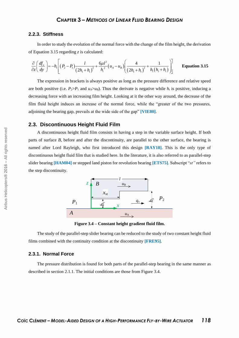
CHAPTER 3 – METHODS OF LINEAR FLUID BEARING DESIGN
COÏC CLÉMENT – MODEL-AIDED DESIGN OF A HIGH-PERFORMANCE FLY-BY-WIRE ACTUATOR 118
2.2.3. Stiffness
In order to study the evolution of the normal force with the change of the film height, the derivation
of Equation 3.15 regarding z is calculated:
2
2 1 2 22
1 11 1
6 4 1
2 2
xt A B
t tt t
df l lh P P u u
z dy h h h hh h h h
Equation 3.15
The expression in brackets is always positive as long as the pressure difference and relative speed
are both positive (i.e. P2>P1 and uA>uB). Thus the derivate is negative while ht is positive, inducing a
decreasing force with an increasing film height. Looking at it the other way around, the decrease of the
film fluid height induces an increase of the normal force, while the “greater of the two pressures,
adjoining the bearing gap, prevails at the wide side of the gap” [VIE80].
2.3. Discontinuous Height Fluid Film
A discontinuous height fluid film consists in having a step in the variable surface height. If both
parts of surface B, before and after the discontinuity, are parallel to the other surface, the bearing is
named after Lord Rayleigh, who first introduced this design [RAY18]. This is the only type of
discontinuous height fluid film that is studied here. In the literature, it is also referred to as parallel-step
slider bearing [HAM04] or stepped land piston for revolution bearing [ETS75]. Subscript “st” refers to
the step discontinuity.
P1x
z
h2 P2
uB
uA
qx
A
Bl l
h1
xst
Figure 3.4 – Constant height gradient fluid film.
The study of the parallel-step slider bearing can be reduced to the study of two constant height fluid
films combined with the continuity condition at the discontinuity [FRE95].
2.3.1. Normal Force
The pressure distribution is found for both parts of the parallel-step bearing in the same manner as
described in section 2.1.1. The initial conditions are those from Figure 3.4.
Airb
us H
elic
opte
rs®
2016 –
All
rights
reserv
ed
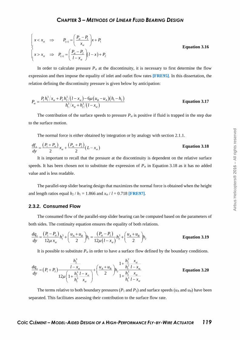
CHAPTER 3 – METHODS OF LINEAR FLUID BEARING DESIGN
COÏC CLÉMENT – MODEL-AIDED DESIGN OF A HIGH-PERFORMANCE FLY-BY-WIRE ACTUATOR 119
1( ) 1
2( ) 2
stst x
st
stst x
st
P Px x P x P
x
P Px x P l x P
l x
Equation 3.16
In order to calculate pressure Pst at the discontinuity, it is necessary to first determine the flow
expression and then impose the equality of inlet and outlet flow rates [FRE95]. In this dissertation, the
relation defining the discontinuity pressure is given below by anticipation:
3 3
1 1 2 2 1 2
3 3
1 2
6st st B A
st
st st
P h x P h l x u u h hP
h x h l x
Equation 3.17
The contribution of the surface speeds to pressure Pst is positive if fluid is trapped in the step due
to the surface motion.
The normal force is either obtained by integration or by analogy with section 2.1.1.
1 2
2 2
st stxst st
P P P Pdfx L x
dy
Equation 3.18
It is important to recall that the pressure at the discontinuity is dependent on the relative surface
speeds. It has been chosen not to substitute the expression of Pst in Equation 3.18 as it has no added
value and is less readable.
The parallel-step slider bearing design that maximizes the normal force is obtained when the height
and length ratios equal h2 / h1 = 1.866 and xst / l = 0.718 [FRE97].
2.3.2. Consumed Flow
The consumed flow of the parallel-step slider bearing can be computed based on the parameters of
both sides. The continuity equation ensures the equality of both relations.
3 31 2
1 1 2 212 2 12 2
st stx A B A B
st st
P P P Pdq u u u uh h h h
dy x l x
Equation 3.19
It is possible to substitute Pst in order to have a surface flow defined by the boundary conditions.
3 2
2 2
2
11 2 2 33
223311
1
2112 1
st
x A Bst st
stst
stst
h h x
dq u ul x h l xP P h
h xdy h l x
h l xh x
Equation 3.20
The terms relative to both boundary pressures (P1 and P2) and surface speeds (uA and uB) have been
separated. This facilitates assessing their contribution to the surface flow rate.
Airb
us H
elic
opte
rs®
2016 –
All
rights
reserv
ed

CHAPTER 3 – METHODS OF LINEAR FLUID BEARING DESIGN
COÏC CLÉMENT – MODEL-AIDED DESIGN OF A HIGH-PERFORMANCE FLY-BY-WIRE ACTUATOR 120
2.3.3. Stiffness
In order to study the evolution of the normal force with the decrease of the film height, the
derivation of Equation 3.18 regarding z is computed:
2
2
2 212 13 2
2 13
1
13
9 12
1
x stB A
st st st
st
h
df l h h xhP P u u l
h xz dy l x h l x
h l x
Equation 3.21
The expression in brackets is always positive as long as the pressure difference and the speed sum
are both positive (i.e. P2>P1 and uB>uA). Thus, the decrease of the film fluid height induces an increase
of the normal force as long as the highest pressure is on the wide side of the parallel-step bearing, as for
constant height gradient bearings.
2.4. Solution Selection
Three manners to generate a normal force in fluid films have been studied in this section. These
first approaches neglected lateral flows. Concrete application for aerospace actuation requires
considering such flow.
However, the literature shows that parallel-step piston normal force is optimistic when discarding
the lateral flow [VOL72]. It has therefore here been decided to focus only on the two other solutions for
the rest of this chapter.
Fluid bearing integration in aerospace actuators is studied as substitution of conventional seals on
pistons and bushings. In both applications, relative speed and pressure difference are involved.
Therefore, the bearing could be referred to as hybrid. However, the term hydrostatic is abusively used
as actuator speeds are low regarding the maximum bearing capability.
Airb
us H
elic
opte
rs®
2016 –
All
rights
reserv
ed

CHAPTER 3 – METHODS OF LINEAR FLUID BEARING DESIGN
COÏC CLÉMENT – MODEL-AIDED DESIGN OF A HIGH-PERFORMANCE FLY-BY-WIRE ACTUATOR 121
dqx /dyP1
x
z
h P2
uB
uAA
B
l l
1 2
2
xP Pdf
ldy
31 2
12 2
x A BP Pdq u u
h hdy l
No stiffness as long as the boundary pressures do not vary with the film height.
P1x
zh
(x) P2
uB
uA
qx
A
B
l l
h2
h1
ht
2
1 11 2 1 2
1 1 1
6 2ln
2 2
x t tA B
t t t
df h h l h hP P P l u u
dy h h h h h h ht
1 2
2 22 12 1
1 16 1 1
A Bx
t
u udq P P
dy h hl h h h
2
2 1 2 22
1 11 1
6 4 1
2 2
xt A B
t tt t
df l lh P P u u
z dy h h h hh h h h
P1x
z
h2 P2
uB
uA
qx
A
Bl l
h1
xst
1 2
2 2
st stxst st
P P P Pdfx L x
dy
3 2
2 2
2
11 2 2 33
223311
1
2112 1
st
x A Bst st
stst
stst
h h x
dq u ul x h l xP P h
h xdy h l x
h l xh x
2
2 1 2 22 13 2
12 1
1 39 1
21
x stB A
st stst st
df h h l h h xP P u u l
z dy l x h l xh h x l x
Table 3.1 – Influence of the linear fluid bearing shape on its main design criteria.
Airb
us H
elic
opte
rs®
2016 –
All
rights
reserv
ed
CHAPTER 3 – METHODS OF LINEAR FLUID BEARING DESIGN
COÏC CLÉMENT – MODEL-AIDED DESIGN OF A HIGH-PERFORMANCE FLY-BY-WIRE ACTUATOR 122
3. DESIGN OF HYDROSTATIC THRUST BEARINGS UNDER AEROSPACE
CONSTRAINTS
3.1. Background
In the common design approach of hydrostatic thrust bearings, the fluid viscosity is assumed to be
constant for defining the fluid film thickness at the lands level, which offers the best combination of
load capability, flow consumption and stiffness [NIC95]. The thrust bearing is thus optimized for a
given operating temperature. This applies well to industrial applications where the fluid temperature is
regulated within a narrow range.
As mentioned above, stiffness of the bearing is achieved by inserting a fixed hydraulic resistance
– usually an orifice or a capillary tube – between the pressure source (ideally constant) and the bearing
recess. In many embedded systems, neither the capillary tube nor the orifice meets the required
performances over the extended range of temperature. On the one hand, the stiffness of the fluid bearing
based on orifice design reduces too much at low temperatures. On the other hand, the consumed flow of
the capillary tube design is excessive at high temperatures. An interesting alternative consists in using a
short tube orifice (STO) that enables the laminar to turbulent transition to be managed by adequate sizing
of its dimensions (diameter and length, typically).
Note 3.3: This section uses knowledge about the capillary tube, orifice and variation of fluid
properties with temperature. These pre-requisites are given in Chapter 2 and in [COI16a].
Note 3.4: In the present developments, the pressures indicated are gauge pressures.
3.2. Temperature Sensitivity
Most applications being industrial, cooling systems can be introduced to the hydraulic circuit to
guarantee an operation near a single functioning point. Therefore, the design of a hydrostatic thrust
bearing is usually optimized for a single operating point defined by temperature, bearing clearance and
recess pressure ( T0, h0 and Pr0 – the subscript 0 refers to the design point for all parameters and variables
in this dissertation). However, for power embedded systems the design is not so simple: the temperature
range varies widely, typically by more than 150°C. This has been emphasized in Chapter 2 during the
development of the fluid model. The sensitivity of the hydrostatic thrust bearing performance to
temperature shall thus be assessed.
Some authors commented that the recess pressure of the thrust bearing, which impacts all the
performances, is unchanged when the hydraulic restriction is of the capillary tube type. In contrast, the
recess pressure is affected in case of use of an orifice [ROW83].
Airb
us H
elic
opte
rs®
2016 –
All
rights
reserv
ed

CHAPTER 3 – METHODS OF LINEAR FLUID BEARING DESIGN
COÏC CLÉMENT – MODEL-AIDED DESIGN OF A HIGH-PERFORMANCE FLY-BY-WIRE ACTUATOR 123
This is understandable as the flows in the capillary tube and in the land are both laminar. In this
case, they are equally related to the change of fluid characteristics, making, ceteris paribus, the recess
pressure constant. This recess pressure only varies with the bearing clearance for a given supply
pressure. For a hydrostatic thrust bearing with a capillary tube, the normalized recess pressure
( βcap = Pr / Ps ), defined with reference to the supply pressure ( Ps ), is given by Equation 3.22. The
parameter β0 corresponds to the value of the normalized recess pressure at the design point.
3
0 0 0
1
1 1cap
h h
Equation 3.22
On its side, the orifice is designed to behave as a turbulent restriction which reacts differently to
temperature variation than the bearing lands. As long as the turbulent pattern is satisfied, the orifice flow
is only impacted by the fluid density, which is much less sensitive to temperature than viscosity.
In a design based on orifice as fixed restriction, the normalized recess pressure βorif, can be
expressed by application of the mass conservation theorem:
6 2 2
0 1 0orif T P orifh h C C
Equation 3.23
with CT and CP being two coefficients as defined below. The first one varies with the temperature
while the second one is a constant defined by the recess pressure at design point:
0
0TC
Equation 3.24
2
0
01PC
Equation 3.25
It is relevant to notice that CT also depends on oil pressure. However, the variation of dynamic
viscosity and density due to oil pressure is negligible regarding the variation with the oil temperature.
The characteristics of a hydrostatic thrust bearing are given as dimensionless equations by Jean
Frêne [FRE95], obtained by division with reference values (subscript “ref”). A constant temperature is
assumed, the normalized reference recess pressure equals one and the reference clearance is the
clearance associated with the design point.
It is proposed here to use the same approach and to introduce the effect of temperature variation on
performance. Therefore, the dimensionless static bearing force30 ( W ), the consumed flow ( Q ) and the
stiffness ( ) become respectively:
30 In the generic study, the fluid film normal force was named fx . By contrast, the fluid bearing force is called W.
Airb
us H
elic
opte
rs®
2016 –
All
rights
reserv
ed

CHAPTER 3 – METHODS OF LINEAR FLUID BEARING DESIGN
COÏC CLÉMENT – MODEL-AIDED DESIGN OF A HIGH-PERFORMANCE FLY-BY-WIRE ACTUATOR 124
W
with ref s wW P S K
Equation 3.26
3
0
0
hQ
h
3
0
0
with s wref
P h KQ
Equation 3.27
03 (1 )cap cap cap
h
h
0
with w sref
S K P
h
Equation 3.28
0(1 )
6(2 )
orif
orif oriforif
h
h
Equation 3.29
where:
S is the bearing surface (pad and recess) [m²]
Kw = W/(Pr S) is the load coefficient [-]
In Equation 3.26 and Equation 3.27, β has to be substituted by its expression obtained from
Equation 3.22 or Equation 3.23 depending on the type of hydraulic fixed restriction (capillary tube or
orifice). It is worth mentioning that:
only the dimensionless flow rate is explicitly impacted by the temperature (through viscosity),
when the restriction is made of a capillary tube, β does not depend on the temperature and,
therefore, does not affect the static bearing force and stiffness. However, the flow rate increases
drastically with temperature,
when an orifice is used, the scheme is inverted. When the temperature increases, the static force
and stiffness vary hugely (due to CT ) while the flow increases slowly, due to an implicit counter-
effect of the dimensionless recess pressure.
3.3. A New Type of Fixed Restriction – The Short Tube Orifice
3.3.1. Characteristics of Ideal Fixed Restriction
When thrust bearings are used in an embedded hydraulic power system, their integration induces
specific constraints and requirements: energy consumption must be minimized, static bearing force and
stiffness must be greater than the minimum specified value for the entire range of temperature.
Therefore, the bearing design based on an orifice is not acceptable because of its low stiffness at low
temperatures. Unfortunately, the design based on capillary tube is not acceptable either, due to its
excessive flow rate at high temperatures.
For this particular need, an “ideal” hydraulic restriction should:
operate under laminar flow conditions at low temperatures,
operate under turbulent flow conditions at high temperatures,
enable selecting by design the temperature at which the transition between laminar and turbulent
flow conditions occurs.
Airb
us H
elic
opte
rs®
2016 –
All
rights
reserv
ed
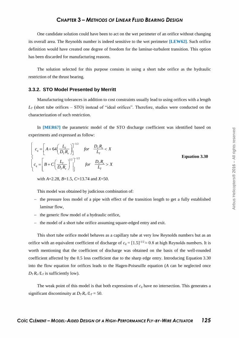
CHAPTER 3 – METHODS OF LINEAR FLUID BEARING DESIGN
COÏC CLÉMENT – MODEL-AIDED DESIGN OF A HIGH-PERFORMANCE FLY-BY-WIRE ACTUATOR 125
One candidate solution could have been to act on the wet perimeter of an orifice without changing
its overall area. The Reynolds number is indeed sensitive to the wet perimeter [LEW62]. Such orifice
definition would have created one degree of freedom for the laminar-turbulent transition. This option
has been discarded for manufacturing reasons.
The solution selected for this purpose consists in using a short tube orifice as the hydraulic
restriction of the thrust bearing.
3.3.2. STO Model Presented by Merritt
Manufacturing tolerances in addition to cost constraints usually lead to using orifices with a length
LT (short tube orifices – STO) instead of “ideal orifices”. Therefore, studies were conducted on the
characterization of such restriction.
In [MER67] the parametric model of the STO discharge coefficient was identified based on
experiments and expressed as follow:
1 2
1 21 2
64 T T eq
T e T
T T eq
T e T
L D Rc A for X
D R L
L D Rc B C for X
D R L
Equation 3.30
with A=2.28, B=1.5, C=13.74 and X=50.
This model was obtained by judicious combination of:
the pressure loss model of a pipe with effect of the transition length to get a fully established
laminar flow,
the generic flow model of a hydraulic orifice,
the model of a short tube orifice assuming square-edged entry and exit.
This short tube orifice model behaves as a capillary tube at very low Reynolds numbers but as an
orifice with an equivalent coefficient of discharge of cq = [1.5]-1/2 ≈ 0.8 at high Reynolds numbers. It is
worth mentioning that the coefficient of discharge was obtained on the basis of the well-rounded
coefficient affected by the 0.5 loss coefficient due to the sharp edge entry. Introducing Equation 3.30
into the flow equation for orifices leads to the Hagen-Poiseuille equation (A can be neglected once
DT Re /LT is sufficiently low).
The weak point of this model is that both expressions of cq have no intersection. This generates a
significant discontinuity at DT Re /LT = 50.
Airb
us H
elic
opte
rs®
2016 –
All
rights
reserv
ed

CHAPTER 3 – METHODS OF LINEAR FLUID BEARING DESIGN
COÏC CLÉMENT – MODEL-AIDED DESIGN OF A HIGH-PERFORMANCE FLY-BY-WIRE ACTUATOR 126
3.3.3. New CFD-Based Model
The approach presented here is based on an adaptation of the former short tube orifice model
considering the following requirements:
1. the model shall be continuous versus DT Re /LT,
2. the model shall be a derivable function of DT Re /LT,
3. the model parameters shall be identified in virtual experiments of CFD simulations,
4. the constant 64 in Equation 3.30 is maintained as it is needed for the establishment of the Hagen-
Poiseuille equation at low DT Re /LT.
Note 3.5: The two first conditions reduce numerical instability on simulation software.
The first two requirements give the two following relations between A, C and X:
XBA
64 Equation 3.31
XC
128 Equation 3.32
Then, almost 70 CFD simulations of different orifices were run with Fluent©. Each numerical
experiment was defined by the value of the DT Re /LT factor, the diameter ( DT ) and the length ( LT ) of
the STO, the pipe diameter ( D0 – upstream of the STO) and the fluid temperature. For manufacturing
considerations, the entrance of the STO was assumed to be conical with a 118° cone angle instead of a
square edge entry as for Merritt’s model.
A design domain has been defined. Numerical experiments consider Reynolds numbers varying
from 10 to 30000, the ratio LT / DT from 1 to 20 and the temperature covering the operating domain
defined in AIR1362 for fluid MIL-PRF-83282 [SAE00], typically from -40°C to +205°C.
(a) – Scheme with nomenclature (b) – CFD mesh (bottom) and pressure (top)
Figure 3.5 – STO views for CFD simulation.
The CFD model was run imposing the downstream pressure and the upstream flow. The STO was
meshed with 34,000 cells, K-epsilon was used as turbulent model and the wall was represented by the
standard model. The flow coefficient value was then identified from the simulated upstream pressure,
Airb
us H
elic
opte
rs®
2016 –
All
rights
reserv
ed

CHAPTER 3 – METHODS OF LINEAR FLUID BEARING DESIGN
COÏC CLÉMENT – MODEL-AIDED DESIGN OF A HIGH-PERFORMANCE FLY-BY-WIRE ACTUATOR 127
according to Equation 3.23. This modus operandi allows for easy simulation of several STO geometries
for a given DT Re /LT factor.
As first conclusions, the pressure drop is almost independent of the pipe-to-STO diameters ratio
( D0 / DT ); the induced variation of cq is in an order of 10-3, which is perfectly negligible.
Then, for a given value of the DT Re /LT parameter, the variation of temperature also has an impact
that is in the order of magnitude of the CFD simulation error and will no longer be considered for the cq
calculation.
Finally, the A, B, C and X values of the parametric model are identified using least square regression
in order to adapt the model as much as possible to the simulations results. The new values specific to
this STO are A=3.22, B=1.35, C=21.86 and X=35.
Figure 3.6 shows the former STO model and its discontinuity at the DT Re /LT transition. The CFD
results and the new model are also plotted with Wuest and Von Misses asymptotes. For better
readability, the new model is represented by a dotted line.
Figure 3.6 – Comparison of flow coefficients
from CFD, Merritt model and the proposed new STO model.
Two main remarks can be made.
The values of the flow coefficient differ slightly from the former model. This is due to the shape
of the entrance of the STO model (cone with an angle of 118°) that is not a sharp-edge entry.
Parameter B of Equation 3.30 now equals 1.35 instead of 1.5.
The STO shape is also the reason why both models are not overlapping for the values of DT Re /LT
from 10 to almost 1000.
Airb
us H
elic
opte
rs®
2016 –
All
rights
reserv
ed

CHAPTER 3 – METHODS OF LINEAR FLUID BEARING DESIGN
COÏC CLÉMENT – MODEL-AIDED DESIGN OF A HIGH-PERFORMANCE FLY-BY-WIRE ACTUATOR 128
It is interesting to note that the Wuest and Von Misses asymptotes intersect near DT Re /LT = 47,
while Merritt gives the value 50 and for the proposed model it is 35.
It also is worth mentioning that if the intention had been to establish the new model, which is
continuous and derivable, from plotted data presented in Merritt (square edge entry) [MER67], the
parameter values truncated after two decimals would have been A=2.24, B=1.5, C=13.75 and X=86.67.
3.3.4. Use of STO as Fixed Orifice for Hydrostatic Thrust Bearings
As defined in Equation 3.26 to Equation 3.29, the static bearing force, the flow and the bearing
stiffness are highly related to the recess pressure. Therefore, the expression of the normalized recess
pressure of the STO-based bearing must be identified.
The Reynolds number is the only variable of the new model of the STO flow coefficient. As it is
function of the flow and used for the flow calculation, an algebraic loop must be solved. Fortunately, in
the particular case of hydrostatic thrust bearings, some considerations can help:
the ratio DT /LT is directly linked to the Reynolds number at the design point,
the flow coefficient is thus only function of the ratio of the Reynolds number at the design point
( Re0 ) and at the point of study ( Re ),
the flow at the STO is considered to be equal to the flow on the lands. Therefore, the laminar
equation can be used for the Reynolds calculation at the STO.
These considerations lead to the new expression that enables the algebraic loop to be removed:
3
2 0 01TT
T e
L hC
D R X h
Equation 3.33
The inclusion of Equation 3.30 – considering Equation 3.33 – into the flow equation for an orifice
provides the flow through the STO. Equalling it to the flow on the lands allows the determination of the
normalized recess pressure. This pressure is consequently defined by one of the two following equations,
depending on the value of DT Re /LT:
6 3
2 2 2
00 0
6 4.5
2 1.5 2
00 0
1 1 064 64
1 1 0
T eT T P
T
T eT T P
T
D RAX h h AXC C C for X
h h L
D RB X h h B XC C C for X
C h h C L
Equation 3.3
4
Unfortunately, solving both parts of Equation 3.34 in order to get an analytical expression of the
normalized recess pressure is not obvious. The recess pressure is thus calculated numerically.
Consequently, the equation of the stiffness of an STO design-based hydrostatic thrust bearing is not
presented. The bearing stiffness indeed equals the partial derivative of the static bearing force regarding
Airb
us H
elic
opte
rs®
2016 –
All
rights
reserv
ed

CHAPTER 3 – METHODS OF LINEAR FLUID BEARING DESIGN
COÏC CLÉMENT – MODEL-AIDED DESIGN OF A HIGH-PERFORMANCE FLY-BY-WIRE ACTUATOR 129
the clearance [FRE95]. To be conservative, the STO stiffness considered in the following is the
minimum value obtained from the calculations based on Equation 3.28 and Equation 3.29, using the
STO recess pressure. This can be justified as the STO should have a behaviour confined by the capillary
tube and orifice responses. In practice, the stiffness based on the capillary tube is always the lowest one,
considering equal normalized recess pressures.
3.4. Pre-Sizing Optimization
3.4.1. Optimization Process
It is proposed to initialize the pre-sizing process of a STO-based hydrostatic thrust bearing by using
the design point ( T0, h0 and β0 ) which corresponds to DT Re0 /LT = 35. Such a point appears “naturally”
in the model as the transition between laminar and turbulent flow conditions.
It is worth mentioning that the recess pressure expressed in Equation 3.34 only depends on:
the design point ( T0, h0 and β0 ),
the temperature of study ( T ) that impacts CT,
the clearance of study ( h ).
In order to simplify the presentation of the pre-sizing process, the optimization will be set around
a particular clearance ( h / h0 = 1 ). It is indeed easiest to understand the study by plotting the
requirements and results in 2D graphs. Considering h as a variable would have added a third dimension.
Criteria function G has to minimize normalized flow Q by action on vector Θ, under the vector of
inequality constraints {c} over the entire temperature range.
0 0 0
min 1
min 2
min
, ,
1;1 ,
J Q
T h
W W cT
c
With the dimensionless temperature defined as follow:
2
2
max min
max min
T TT
TT T
Equation 3.35
The optimization is made possible by action on the design point. As mentioned above, the pre-
design process is run around the design point clearance ( h / h0 = 1 ). Therefore, the design point is only
defined by its temperature and recess pressure ( T0 and β0 ).
Airb
us H
elic
opte
rs®
2016 –
All
rights
reserv
ed

CHAPTER 3 – METHODS OF LINEAR FLUID BEARING DESIGN
COÏC CLÉMENT – MODEL-AIDED DESIGN OF A HIGH-PERFORMANCE FLY-BY-WIRE ACTUATOR 130
3.4.2. Optimized Pre-Sizing
The objective is to design a hydrostatic thrust bearing satisfying the following performance
requirements for the entire range of temperature:
a dimensionless static load higher than 0.2
a dimensionless consumed flow lower than 1
a dimensionless stiffness higher than 0.4
The three types of hydraulic restriction – orifice, capillary tube and short tube orifice – are
compared using the temperature at the design point as an optimization parameter. The results are
presented in Figure 3.7, Figure 3.8 and Figure 3.9 for each restriction, depending on the temperature.
The striped zone indicates the limit of the performance requirement.
Figure 3.7 – Dimensionless static bearing force versus fluid temperature.
The dimensionless static forces of the bearings using the three different hydraulic restrictions are
acceptable. The sensitivity of the STO to temperature is lower than that of the orifice but still much
higher than that of the capillary tube.
If the static force requirement had not been met, the optimization would have tried to obtain a
higher temperature value for the design point. This would have led to a wider range of constant static
bearing forces, and thus to a higher force when the dimensionless temperature equals one. Of course,
this is possible only if the other constraints are also satisfied.
Airb
us H
elic
opte
rs®
2016 –
All
rights
reserv
ed

CHAPTER 3 – METHODS OF LINEAR FLUID BEARING DESIGN
COÏC CLÉMENT – MODEL-AIDED DESIGN OF A HIGH-PERFORMANCE FLY-BY-WIRE ACTUATOR 131
Figure 3.8 – Dimensionless bearing flow rate versus fluid temperature.
As expected, the dimensionless flow rate is slightly lower for an STO than for the orifice below the
temperature of the design point and almost similar for greater values. The capillary tube cannot be
selected for this embedded system application due to the high flow rate, which is more than twice the
requirement value.
Finally, the stiffness of the bearing with STO is compliant with the requirement as it behaves as a
capillary tube once the flow has been established as perfectly laminar.
Figure 3.9 – Dimensionless bearing stiffness versus fluid temperature.
The compromise of the STO as hydraulic restriction for hydrostatic thrust bearings is a lower
stiffness than the orifice around the design point temperature. However, this is perfectly acceptable as
the more constraining point is at low temperatures.
Airb
us H
elic
opte
rs®
2016 –
All
rights
reserv
ed
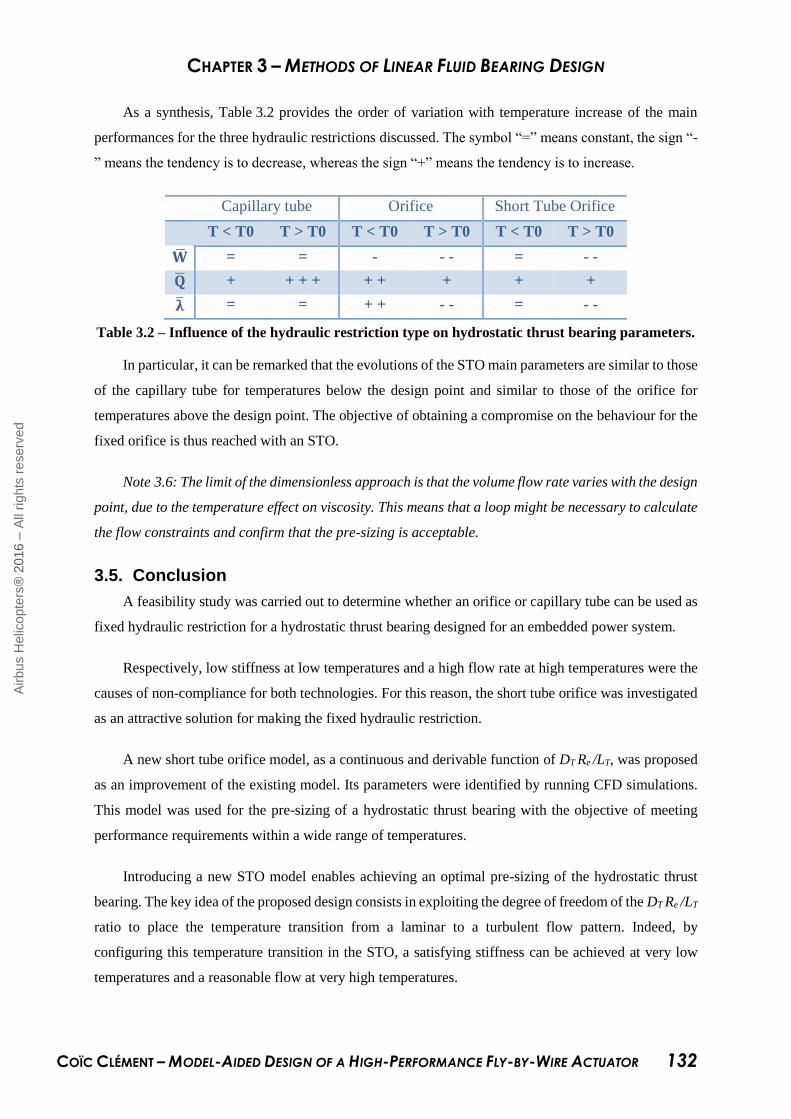
CHAPTER 3 – METHODS OF LINEAR FLUID BEARING DESIGN
COÏC CLÉMENT – MODEL-AIDED DESIGN OF A HIGH-PERFORMANCE FLY-BY-WIRE ACTUATOR 132
As a synthesis, Table 3.2 provides the order of variation with temperature increase of the main
performances for the three hydraulic restrictions discussed. The symbol “=” means constant, the sign “-
” means the tendency is to decrease, whereas the sign “+” means the tendency is to increase.
Capillary tube Orifice Short Tube Orifice
T < T0 T > T0 T < T0 T > T0 T < T0 T > T0
�̅� = = - - - = - -
�̅� + + + + + + + + +
�̅� = = + + - - = - -
Table 3.2 – Influence of the hydraulic restriction type on hydrostatic thrust bearing parameters.
In particular, it can be remarked that the evolutions of the STO main parameters are similar to those
of the capillary tube for temperatures below the design point and similar to those of the orifice for
temperatures above the design point. The objective of obtaining a compromise on the behaviour for the
fixed orifice is thus reached with an STO.
Note 3.6: The limit of the dimensionless approach is that the volume flow rate varies with the design
point, due to the temperature effect on viscosity. This means that a loop might be necessary to calculate
the flow constraints and confirm that the pre-sizing is acceptable.
3.5. Conclusion
A feasibility study was carried out to determine whether an orifice or capillary tube can be used as
fixed hydraulic restriction for a hydrostatic thrust bearing designed for an embedded power system.
Respectively, low stiffness at low temperatures and a high flow rate at high temperatures were the
causes of non-compliance for both technologies. For this reason, the short tube orifice was investigated
as an attractive solution for making the fixed hydraulic restriction.
A new short tube orifice model, as a continuous and derivable function of DT Re /LT, was proposed
as an improvement of the existing model. Its parameters were identified by running CFD simulations.
This model was used for the pre-sizing of a hydrostatic thrust bearing with the objective of meeting
performance requirements within a wide range of temperatures.
Introducing a new STO model enables achieving an optimal pre-sizing of the hydrostatic thrust
bearing. The key idea of the proposed design consists in exploiting the degree of freedom of the DT Re /LT
ratio to place the temperature transition from a laminar to a turbulent flow pattern. Indeed, by
configuring this temperature transition in the STO, a satisfying stiffness can be achieved at very low
temperatures and a reasonable flow at very high temperatures.
Airb
us H
elic
opte
rs®
2016 –
All
rights
reserv
ed

CHAPTER 3 – METHODS OF LINEAR FLUID BEARING DESIGN
COÏC CLÉMENT – MODEL-AIDED DESIGN OF A HIGH-PERFORMANCE FLY-BY-WIRE ACTUATOR 133
4. DESIGN OF CONICAL HYBRID BEARINGS UNDER AEROSPACE
CONSTRAINTS
4.1. Background
Conical hybrid bearings are well defined in the literature, mainly thanks to Viersma [VIE80]. From
the constant height gradient axial fluid film, integration of the force and flow rate is performed on 360°,
considering a possible piston eccentricity e in the housing. Indeed, the inclusion of eccentricity makes
the fluid heights, h1 and h2, dependent on the azimuth φ (Figure 3.10).
e e
l
d
t
φ
dφ
df
c+e
P1 P2
uB
uA
Figure 3.10 – Geometry and notations of a conical bearing from [VIE80].
The centring force W the conical hybrid bearing is able to provide is thus given, in the direction of
the eccentricity, by:
2 12 2
2 2 2 22
2 2
21
4 2 4
6 2
2 4
t t
t
t tA B
t tt
h l d c hW P P
e c h e
c h e c el d c hu u
h e h c h e
Equation 3.36
The volume flow rate calculated by Viersma neglected the contribution of speed. The reason was
that the leakage flow was much smaller than the displacement flow. This condition is not necessarily
satisfied in our application. Consequently, the contribution of speed to the conical hybrid bearing flow
has been calculated and added to the equation provided by Viersma:
Airb
us H
elic
opte
rs®
2016 –
All
rights
reserv
ed

CHAPTER 3 – METHODS OF LINEAR FLUID BEARING DESIGN
COÏC CLÉMENT – MODEL-AIDED DESIGN OF A HIGH-PERFORMANCE FLY-BY-WIRE ACTUATOR 134
23
2 1
2
2
1 1.75 1.5 112 2
21
2 21
2
t t
t
ttA B
t
c d h h eQ P P
l c c c
h
c hd hu u c
e
c h
Equation 3.37
Finally, the conical hybrid bearing stiffness can be derived from the normal force:
2 1 3 2 2 22 22
2
3 22 2 2 2 22 2
2 2 2 2
2 2 2
2 1 21
4 2 42 4
4 26 1 1
2 4
2
2 4
t tt
tt
t
A B
tt t
tt t
tt
c hW c hP P h l d
e e c h ec h e
t c hl du u
h c e c h e c h e
c h e c eh c h
e h c h e
Equation 3.38
This last equation is obviously not user-friendly, but actually only the speed, pressure, viscosity
and eccentricity values are time variables.
4.2. Temperature and Eccentricity Sensitivity
The dependency on temperature of the three main design criteria (force, flow and stiffness) of the
conical hybrid bearing is less complex than for the hydrostatic bearing. Indeed, the stiffness of the
conical hybrid bearing comes from its tapered shape. This shape provides hydrostatic force, physical
wedge and translational squeeze. Thus, unlike for hydrostatic bearings, no fixed restriction is required
and the only variable affected by the temperature in the three main criteria equations is viscosity. But it
is important to assess the performance variation with temperature for several eccentricities.
The three main criteria are studied for the extended range of temperature and several eccentricities.
The results are presented in Figure 3.11, Figure 3.12 and Figure 3.13. In each of these figures, dashed
lines show the contribution of pressure to the criteria (hydrostatic effect – subscript “hd”), dotted lines
represent the contribution of speed (hydrodynamic effect – subscript “hs”), while the full lines stand for
the combination of both.
Note 3.7: This study is carried out considering the data provided on the design example in [VIE80].
A complete dimensionless study, such as the one carried out in the previous section, is almost impossible
due to the complexity of the formula involved. Sensitivity to design parameters is thus analysed in the
next section.
Airb
us H
elic
opte
rs®
2016 –
All
rights
reserv
ed
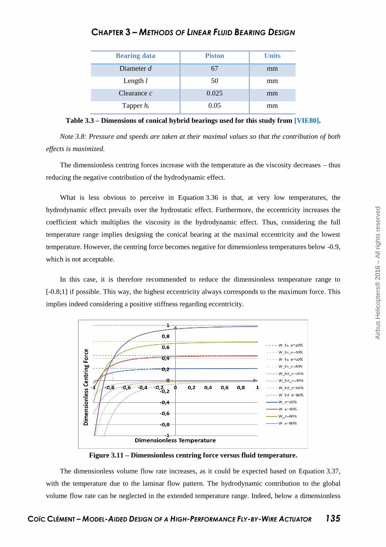
CHAPTER 3 – METHODS OF LINEAR FLUID BEARING DESIGN
COÏC CLÉMENT – MODEL-AIDED DESIGN OF A HIGH-PERFORMANCE FLY-BY-WIRE ACTUATOR 135
Bearing data Piston Units
Diameter d 67 mm
Length l 50 mm
Clearance c 0.025 mm
Tapper ht 0.05 mm
Table 3.3 – Dimensions of conical hybrid bearings used for this study from [VIE80].
Note 3.8: Pressure and speeds are taken at their maximal values so that the contribution of both
effects is maximized.
The dimensionless centring forces increase with the temperature as the viscosity decreases – thus
reducing the negative contribution of the hydrodynamic effect.
What is less obvious to perceive in Equation 3.36 is that, at very low temperatures, the
hydrodynamic effect prevails over the hydrostatic effect. Furthermore, the eccentricity increases the
coefficient which multiplies the viscosity in the hydrodynamic effect. Thus, considering the full
temperature range implies designing the conical bearing at the maximal eccentricity and the lowest
temperature. However, the centring force becomes negative for dimensionless temperatures below -0.9,
which is not acceptable.
In this case, it is therefore recommended to reduce the dimensionless temperature range to
[-0.8;1] if possible. This way, the highest eccentricity always corresponds to the maximum force. This
implies indeed considering a positive stiffness regarding eccentricity.
Figure 3.11 – Dimensionless centring force versus fluid temperature.
The dimensionless volume flow rate increases, as it could be expected based on Equation 3.37,
with the temperature due to the laminar flow pattern. The hydrodynamic contribution to the global
volume flow rate can be neglected in the extended temperature range. Indeed, below a dimensionless
Airb
us H
elic
opte
rs®
2016 –
All
rights
reserv
ed

CHAPTER 3 – METHODS OF LINEAR FLUID BEARING DESIGN
COÏC CLÉMENT – MODEL-AIDED DESIGN OF A HIGH-PERFORMANCE FLY-BY-WIRE ACTUATOR 136
temperature of -0.8, it is comparable to the hydrostatic contribution, but compared to the flow at high
temperatures, both are in the order of 1%. This is consistent with Viersma’s statement [VIE80].
Figure 3.12 – Dimensionless volume flow rate versus fluid temperature.
The bearing should thus be designed considering the maximum eccentricity at the highest
temperature, as this combination induces maximum flow.
Figure 3.13 – Dimensionless stiffness versus fluid temperature.
The dimensionless bearing stiffness declines at low temperatures. With the increase of eccentricity,
this decrease occurs sooner. Depending on the required minimum stiffness, it could be necessary to limit
the bearing force at low temperatures in order to contain the maximum eccentricity.31
31 This possibility makes sense for aeronautic applications where the flight domain can be constrained by the
fluid temperature.
Airb
us H
elic
opte
rs®
2016 –
All
rights
reserv
ed

CHAPTER 3 – METHODS OF LINEAR FLUID BEARING DESIGN
COÏC CLÉMENT – MODEL-AIDED DESIGN OF A HIGH-PERFORMANCE FLY-BY-WIRE ACTUATOR 137
4.3. Design Parameter Sensitivities
For the design of conical hybrid bearings under aerospace constraints, it is reasonable to consider
the pressures, speeds and diameters as inputs. The remaining parameters are the bearing length, taper
height and clearance.
It is of interest to assess their impact on the three main criteria, which are also dependent on the
time variables: temperature and eccentricity. Figure 3.14, Figure 3.15 and Figure 3.16 respectively show
the sensitivity of the three main criteria to the bearing length, the taper height and the ht/c ratio
considering the maximum eccentricity of 0.8. This value corresponds to a fluid film height of 5 µm,
which prevents fluid film rupture.
Note 3.9: In the three figures, the volume flow rate axis is on the right part of the graphs, as the
flow is always positive. This provides a better scaling of the plotted curves. Both the centring force and
stiffness axes are in the centre of the figures.
Note 3.10: On the three figures, one colour is used per parameter value. Full, dotted and dashed
lines respectively show the centring force, bearing stiffness and volume flow rate.
Figure 3.14 – Dimensionless main criteria versus fluid temperature for different bearing lengths.
Increasing the bearing length is tempting as it decreases the volume flow rate and increases the
maximum values of both the centring force and the stiffness. However, caution should be exercised as
it also makes these two criteria fall “sooner” at low temperatures.
Airb
us H
elic
opte
rs®
2016 –
All
rights
reserv
ed
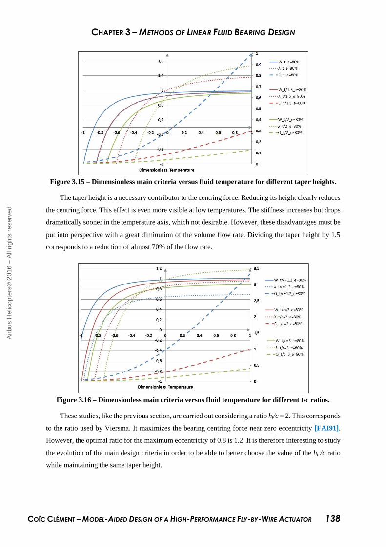
CHAPTER 3 – METHODS OF LINEAR FLUID BEARING DESIGN
COÏC CLÉMENT – MODEL-AIDED DESIGN OF A HIGH-PERFORMANCE FLY-BY-WIRE ACTUATOR 138
Figure 3.15 – Dimensionless main criteria versus fluid temperature for different taper heights.
The taper height is a necessary contributor to the centring force. Reducing its height clearly reduces
the centring force. This effect is even more visible at low temperatures. The stiffness increases but drops
dramatically sooner in the temperature axis, which not desirable. However, these disadvantages must be
put into perspective with a great diminution of the volume flow rate. Dividing the taper height by 1.5
corresponds to a reduction of almost 70% of the flow rate.
Figure 3.16 – Dimensionless main criteria versus fluid temperature for different t/c ratios.
These studies, like the previous section, are carried out considering a ratio ht/c = 2. This corresponds
to the ratio used by Viersma. It maximizes the bearing centring force near zero eccentricity [FAI91].
However, the optimal ratio for the maximum eccentricity of 0.8 is 1.2. It is therefore interesting to study
the evolution of the main design criteria in order to be able to better choose the value of the ht /c ratio
while maintaining the same taper height.
Airb
us H
elic
opte
rs®
2016 –
All
rights
reserv
ed

CHAPTER 3 – METHODS OF LINEAR FLUID BEARING DESIGN
COÏC CLÉMENT – MODEL-AIDED DESIGN OF A HIGH-PERFORMANCE FLY-BY-WIRE ACTUATOR 139
By changing the ratio from 1.2 to 3, the maximum bearing centring force only decreases by 10%,
while the volume flow rate is reduced by a factor 7. Caution should be exercised with respect to stiffness,
which becomes negative at low temperatures, resulting in an attractive force. Thus, if margins are
available on both the centring force and the stiffness at low temperatures, or if the overall extended
range of temperature is not required, it would be convenient to increase this ratio in order to reduce the
leakage.
4.4. Conclusion
The equations providing the three main criteria for a conical hybrid bearing were presented in this
section. While the centring force equation is well-known, the volume flow rate relation was completed
with the contribution of the hydrodynamic effect in this dissertation. The bearing stiffness was derived
from the centring force equation.
In addition, two studies were carried out in this section. Based on a conical bearing design example
proposed by Viersma, the first study assesses the dependency of the three main design criteria on
temperature and eccentricity. For each criterion, the contribution of both the hydrostatic and
hydrodynamic effects was emphasized. A common trend could be revealed. Considering an extended
range of temperature, the characteristics of the three main criteria drop at low temperatures. Even though
this is desirable for the volume flow rate, it can become unacceptable for both the centring force and the
stiffness, for which negative values can be reached.
A second study assessed the sensitivity of the three main design criteria with respect to the three
design parameters. Reducing the bearing length enables increasing the centring force and reducing the
leakage but comes at the cost of low stiffness at low temperatures. A small diminution of the taper height
or an increase of the taper height/clearance ratio are both acceptable options to reduce the leakage
without a dramatic counter-effect on the other performances.
Fluid bearing friction was not addressed as it was not considered to be a key design driver.
Corresponding models are available, e.g.: [SCH97]. Their implementation is proposed as a perspective
to this study.
Airb
us H
elic
opte
rs®
2016 –
All
rights
reserv
ed

CHAPTER 3 – METHODS OF LINEAR FLUID BEARING DESIGN
COÏC CLÉMENT – MODEL-AIDED DESIGN OF A HIGH-PERFORMANCE FLY-BY-WIRE ACTUATOR 140
5. CONCLUSION
Hybrid fluid bearings were identified as a good alternative to current sealing and bearing devices.
At the cost of a contained leakage, a satisfying centring force and bearing stiffness can be obtained.
However, the design of such fluid bearings must be realized with caution. These performances indeed
highly depend on time variables and design parameters.
Therefore, in a first section, the Reynolds equation was presented based on the equilibrium of fluid
elements in a fluid film. The importance of each of its effects was discussed and associated
simplification for our subsequent analysis was proposed.
Based on this simplified Reynolds equation, three different manners to generate a normal force in
a fluid film were investigated in section 2. As a first approach, only the axial flow was considered. The
axial study established three candidates for further investigation: hydrostatic thrust bearings, conical
hybrid bearings and parallel-step piston. It was decided to focus only on the first two solutions as
literature shows that parallel-step piston normal force is less promising than the others.
A pre-sizing process for hydrostatic thrust bearings with special consideration for performance
robustness within an extended range of temperature was developed in section 3. This was made possible
only by introducing a short tube orifice as a fixed restriction. A new STO model was proposed based on
the analytic requirements and parameters identified using CFD simulations. The key idea of the
proposed design consists in exploiting the degree of freedom of the DT Re /LT ratio to place the
temperature transition from a laminar to a turbulent flow pattern. Indeed, configuring this temperature
transition in the STO enables achieving a satisfying stiffness at very low temperatures and a reasonable
flow at very high temperatures.
Finally, section 4 focused on a conical hybrid design under aerospace constraints. The impact of
the time variables and design parameters was assessed. As final recommendation to both designs, it is
important to contain as much as possible the lowest values of the temperature domain in order to
optimize the design. An alternative could be to degrade the performance specified with the decrease of
temperature. However, obtaining satisfying values may prove difficult.
The research performed in this chapter provides input for the high-performance actuator prototype
development detailed in the next chapter (Restricted). Fluid bearings are a key technological step
identified to enhance actuator performance, ensuring a satisfying lifespan.
Airb
us H
elic
opte
rs®
2016 –
All
rights
reserv
ed
CHAPTER 3 – METHODS OF LINEAR FLUID BEARING DESIGN
COÏC CLÉMENT – MODEL-AIDED DESIGN OF A HIGH-PERFORMANCE FLY-BY-WIRE ACTUATOR 141
BIBLIOGRAPHY
[BLA60] BLACKBURN, J.F., REETHOF, G. & SHEARER, J.L., Fluid Power Control. John Wiley &
Sons, Inc., New York and London, 1960.
[COI16a] COÏC C. & MARÉ J.-C., Modeling and Pre-Sizing Process for Hydrostatic Thrust
Bearing with Special Consideration to Performance Robustness within a Wide
Temperature Range, International Conference on Hydraulics and Pneumatics, Praha,
Czech Republic, 2016.
[ETS75] ETSION, I., An Optimum Step Design for Centering of Pistons. ASME, Journal of
Fluids Engineering, 1975.
[FAI83] FAISANDIER, J., Mécanismes Hydrauliques. Dunod, Paris, 1983. (in French)
[FAI91] FAISANDIER, J., GRAND, S., LEBRUN, M. & THOMA, J.U., Hydraulique et Informatique
ou l’Informatique au Service de l’Hydraulique, Promotion Presse Internationale, Paris,
1991. (in French)
[FRE95] FRENE, J., Butées et Paliers Hydrodynamiques. Techniques de l’Ingénieur, B5 320,
1995. (in French)
[FRE97] FRÊNE, J., NICOLAS, D., DEGUEURCE, B., BERTHE, D. & GODET, M., Hydrodynamic
Lubrication: Bearings and Thrust Bearings. Tribology Series, 33, Elsevier, 1997.
[HAM04] HAMROCK, B.J., SCHMID, S.R. & JACOBSON, B.O. Fundamentals of Fluid Flim
Lubrication, Second Edition. Marcel Dekker, Inc., 2004.
[LEW62] LEWIS, E.E. AND STERN, H., Design of Hydraulic Control Systems. McGraw-Hill, 1962.
[MAR93] MARE, J.-C., Contribution à la Modélisation, la Simulation, l’Indentification et la
Commande d’Actionneurs Électrohydrauliques. Thèse d’état, Lyon, 1993. (in French)
[MER67] Merritt, H.E., Hydraulic Control System, John Wiley & sons, Inc., 1967.
[NIC95] NICOLAS, D., Butées et Paliers Hydrostatiques. Techniques de l’ingénieur, b5325,
1995. (in french)
[POS89] POSSAMAI, O., Étude et Conception d’un Guidage Linéaire de Haute Précision à Palier
Fluide. Université de Compiègne, 1989. (in French)
[RAY18] RAYLEIGH, L., Notes on the Theory of Lubrication. Philosophical Magazine, Vol. 35
pp.1-12, 1918.
[REY86] REYNOLDS, O., On the Theory of Lubrication and its Application to Mr. Beauchamp
Tower’s Experiments, including an Experimental Determination of the Viscosity of
Olive Oil. 1886.
[ROW83] ROWE, W.B., Hydrostatic and Hybrid Bearing Design. Butterworths, London, 1983.
[SAE00] S.A.E., AIR 1362 – Aerospace Hydraulic Fluids Physical Properties. USA, 2000.
[SCH14] SCHMID, S.R., HAMROCK, B.J. & JACOBSON, B.O., Fundamentals of Machine
Elements, Third Edition. CRC Press., 2014.
[SCH97] VAN SCHOTHORST, G., Modelling of Long-Stroke Hydraulic Servo-Systems for Flight
Simulator Motion Control and System Design. Netherland, 1997.
[VIE80] VIERSMA, T.J., Analysis, Synthesis and Design of Hydraulic Servosystems and
Pipelines. Elsevier, 1980.
[VOL72] VOLMAN, H.J.W.M., Berekeningen en Constructie van het Radiaal Staplager.
Ploytechn. Tijdschr., 1972.
Airb
us H
elic
opte
rs®
2016 –
All
rights
reserv
ed

CHAPITRE 4 – ACTIONNEUR HYDRAULIQUE DE CONTROLE ACTIF
COÏC CLÉMENT – MODEL-AIDED DESIGN OF A HIGH-PERFORMANCE FLY-BY-WIRE ACTUATOR 142
CONCLUSION GENERALE
Le but de cette thèse était d’étudier la possible augmentation de performances des actionneurs de
commandes de vol électriques pour hélicoptères. En effet, les solutions technologiques assurant
l’étanchéité et le centrage de l’ensemble piston/corps du vérin ne permettent pas l’implémentation de
nouvelles fonctions de pilotage, dû à leur faible durée de vie lorsqu’ils sont soumis à des déplacements
hautes fréquences.
Les paliers fluides linéaires ont été identifiés comme une alternative aux systèmes d’étanchéités
conventionnels afin d’améliorer les performances de l’actionneur, en admettant de légères fuites
internes. Seulement cette substitution technologique ne peut être réalisé sans une totale compréhension
de l’impact que cela aura sur l’actionneur lui-même, le système d’actionnement global et finalement les
commandes de vols et la réponse engendrée sur le comportement de l’hélicoptère.
Il a donc été choisi d’organiser cette recherche selon trois axes principaux contribuant chacun à ce
but final :
1. Présenter les différentes technologies d’actionneurs et synthétiser comment les contraintes
imposées par les commandes de vol impactent leur architecture et le choix technologique associé.
2. Développer une modélisation orientée-objet du système d’actionnement dans le but d’aider le
développement et de permettre un interfaçage avec le système de commandes de vol global.
3. Étudier l’implémentation de paliers fluides linéaires au sein des actionneurs en considérant les
contraintes aéronautiques associées.
Dans la première partie, l’évolution incrémentale des commandes de vol, portée par les besoins
naissants, a été détaillée. Les nouveaux composants, ajoutés chronologiquement aux commandes de vol
conventionnelles, ont été présentés simultanément à la fonction qu’ils remplissent. Cette analyse
fonctionnelle a mis en évidence le besoin de repenser le système (« re-engineering » en anglais) lors du
passage aux commandes de vol électriques. Nous avons introduit une architecture ainsi qu’un
vocabulaire générique afin de décrire les différentes technologies d’actionneurs et supporter leurs
analyses. Nous avons recommandé la technologie d’actionneur électrohydraulique à actionnement direct
du distributeur (DDV) pour les actionneurs de commandes de vol primaires et insisté sur les bénéfices
liés à l’utilisation de la technologie de servovalves électrohydrauliques (EHSV) pour les fonctions non-
critiques telles que certaines commandes de vol secondaires. Nous avons conclu cette partie en
présentant les perspectives d’évolution des commandes de vol dans les décennies à venir.
La deuxième partie de ce mémoire consistait en la modélisation virtuelle et la simulation du système
d’actionnement en utilisant le formalisme Bond-graph. Le développement des modèles virtuels a été
Airb
us H
elic
opte
rs®
2016 –
All
rights
reserv
ed

CONCLUSION GENERALE
COÏC CLÉMENT – MODEL-AIDED DESIGN OF A HIGH-PERFORMANCE FLY-BY-WIRE ACTUATOR 143
conduit en analogie avec la méthode d’Ingénierie Systèmes : définissant les besoins de la modélisation
du point de vue ingénieur et industriel, pensant l’architecture des modèles selon ces besoins et,
finalement, développant chaque sous-modèle en utilisant les principes de l’orientation-objet. Le
formalisme Bond-graph, de par sa généricité multi-domaines physiques, a facilité cette approche. Une
attention particulière a été portée à la compréhensibilité des modèles Bond-graphs en combinant l’état
de l’art en termes de lisibilité et en améliorant la topologie des modèles. Le modèle de fluide, fonction
de la température, permet l’étude du système d’actionnement sur l’ensemble de l’intervalle de
température, nécessaire (car extrêmement contraignant) lors d’un développement aéronautique. Dans
cette partie, nous avons proposé une standardisation des interfaces et des modèles. Les causalités
préférentielles ont été attribuées aux modèles afin de s’affranchir des contraintes liées à
l’implémentation des modèles dans les différents environnements de simulation. Nous avons validé cette
modélisation du système d’actionnement composant par composant à l’aide de tests unitaires ainsi que
dans sa globalité en réalisant des tests d’intégration. Cette modélisation a finalement été interfacée avec
un model global du système de commande de vol dans le but d’aider au choix de l’architecture et du
dimensionnement du système d’actionnement d’un nouvel hélicoptère.
La troisième partie était dédiée à l’étude des paliers fluides linéaires et leur utilisation pour une
application système de puissance embarqué soumis à de sévères contraintes environnementales.
Généralement, les paliers fluides sont utilisés dans un environnement industriel où la température du
fluide est maintenue quasiment constante, contrairement à l’aéronautique où le domaine opérationnel
du fluide inclus une plage de température de plus de 150°C. Considérant trois différentes technologies
de paliers fluides, il a été détaillé comment celles-ci généraient un effort de centrage, une raideur radiale
au prix d’une faible fuite. L’étude de la littérature existante nous a permis de sélectionner les butées
hydrostatiques ainsi que les paliers hybrides fluides comme potentiels candidats à notre application.
Nous avons décrit une méthode de pré-dimensionnement de la première solution technologique en
utilisant un « orifice tube-court » comme restriction fixe. Nous avons en effet proposé d’influencer par
design la température de transition de l’écoulement laminaire-turbulent dans l’orifice tube-court. Ceci
était un élément clé pour obtenir des performances satisfaisantes en terme de force de centrage et de
raideur tout en limitant le débit de fuite – ce qui n’aurait pas été possible en utilisant un orifice
conventionnel ou un tube capillaire. Concernant les paliers coniques hybrides, nous avons conduit une
étude de sensibilité afin d’observer l’impact des paramètres de design et des variables temporelles sur
les principaux critères d’intérêt. Cela a révélé des raideur et effort de centrage du palier et inacceptables
aux faibles températures, majoritairement dus à l’augmentation exponentielle de la viscosité du fluide.
Finalement, nous avons recommandé de maintenir autant que faire se peut l’intervalle opérationnel de
température dans le but d’optimiser le design des paliers fluides linéaires.
Airb
us H
elic
opte
rs®
2016 –
All
rights
reserv
ed
CONCLUSION GENERALE
COÏC CLÉMENT – MODEL-AIDED DESIGN OF A HIGH-PERFORMANCE FLY-BY-WIRE ACTUATOR 144
La quatrième et dernière partie de ce mémoire était dédiée au développement d’un actionneur haute
performances pour le contrôle actif de rotor avec l’aide de modèles virtuels. Elle se base sur les trois
axes principaux investigués précédemment. La définition de l’architecture de l’actionneur, portée par
les contraintes de sûreté, ainsi que le choix de technologies d’actionneur de commandes de vol
électriques ont été réalisés sur la base des résultats du premier axe de ce mémoire. L’amélioration des
performances tout en conservant une durée de vie acceptable a été possible grâce à l’utilisation de paliers
hybrides coniques. La modélisation Bond-graph proposée a aidé le pré-dimensionnement de
l’actionneur et a permis de vérifier son comportement par simulation virtuelle. Un prototype physique a
été produit et est actuellement en période de tests sur des bancs d’essais dédiés.
Plusieurs améliorations possibles ont été identifiés et laissés en tant que perspectives des travaux
effectués. Nous les avons organisés en deux axes principaux :
1. Les perspectives s’inscrivant dans les trois axes listés auparavant.
2. Les perspectives relatives à l’implémentation de ces axes au niveau de l’actionneur.
En analogie avec le développement d’un produit, le premier point correspondrait aux perspectives
unitaires alors que le second serait les perspectives d’intégration. La priorisation des perspectives
dépendrait par contre des besoins d’Airbus Helicopters et des contraintes de planning liés aux
développements en cours. Cela diverge d’un cycle en V dans un schéma d’ingénierie systèmes où les
tests unitaires devraient être conduits avant les tests d’intégration.
Nous avons identifié en tant que perspectives unitaires :
- Détailler le design « Top-Down » des différentes technologies d’actionneurs. Dans ce mémoire,
les technologies ont été présentés sur la base de solution existante, c’est une approche dite
« Bottom-Up ». Ceci ne permet pas de garder une trace de quelles architectures ont été écartées
dans le développement ni les raisons de ces choix. Une approche descendante, depuis une
spécification technique complète et en suivant une méthodologie d’ingénierie systèmes, pourrait
mener à l’élaboration d’un outil permettant la sélection systématique d’architecture.
- Développer une modélisation thermo-hydraulique du système d’actionnement. La modélisation
actuelle permet de modifier la température du système en fonction du temps de simulation mais
est homogène dans la totalité du circuit. Ceci peut être atteint dans le formalisme Bond-graph en
propageant quatre variables – le débit massique, la pression, la température et l’enthalpie – en lieu
et place des variables d’hydraulique de puissance – le débit volumique et la pression. Il est
toutefois à noter qu’augmenter le réalisme de la modélisation hydraulique à ce niveau n’a de sens
que si le modèle détaillé de l’environnement du système est disponible.
Airb
us H
elic
opte
rs®
2016 –
All
rights
reserv
ed
CONCLUSION GENERALE
COÏC CLÉMENT – MODEL-AIDED DESIGN OF A HIGH-PERFORMANCE FLY-BY-WIRE ACTUATOR 145
- Investiguer le diagnostic de fautes des composants du système d’actionnement sur la base de
l’analyse structurelle de la modélisation Bond graph. Cette étude pourrait être séparée en deux
parties : la première permettrait de déterminer quelles fautes peuvent être détectées en utilisant
les capteurs déjà présents à bord de l’hélicoptère, alors que la deuxième consisterait à déterminer
les capteurs à ajouter afin de pouvoir détecter de nouvelles fautes. Une attention particulière devra
être porté à l’isolation des fautes de manière à éviter les détections intempestives.
- Augmenter le niveau de réalisme du modèle mécanique en utilisant les Multi-Bonds dans le but
de représenter tous les degrés de libertés des parties mécaniques. Ceci permettrait notamment de
modéliser les interactions entre plusieurs axes. Pour donner un exemple, l’excentricité du piston
par rapport au corps du vérin n’a pas été modélisé dynamiquement dans ces recherches dû aux
limitation en terme de mouvement 3D du modèle.
- Développer des modèles de paliers fluides en incluant les notions de frictions et de centre de
pression. Cette perspective est dépendante de la précédente. En effet, les paliers fluides génèrent
des efforts normaux et de translation qui requièrent une modélisation multiaxe. L’effort de
centrage est la force résultante du champ de pression ramenée au centre de pression.
Nous avons identifié, en tant que perspectives d’intégration les points suivants laissés pour des
études futures :
- Conduire une analyse de sensibilité des tolérances de fabrication de paliers fluides. La production
en série d’un actionneur hautes performances ne pourra démarrer uniquement si la répétabilité
des performances est démontrée. Une amélioration possible du design de l’actionneur pourrait
consister à usiner les paliers en tant que pièces séparées du piston ou corps du vérin et de les
assembler en utilisant des joints statiques. Cette solution permettrait l’appairage des pièces qui,
bien que coûteux, réduirait l’intervalle de variation du jeu au niveau des paliers et donc le débit
de fuite interne.
- Analyser les résultats d’essai et vérifier le pré-dimensionnement et la modélisation de l’actionneur
haute-performances. La modélisation du système d’actionnement a été vérifiée en utilisant des
données de vol réelles enregistrées. Pour autant, l’introduction de nouveaux paramètres de
l’actionneur haute performance peut être erronée ou, potentiellement, un effet physique négligé
pour les actionneurs conventionnels joue un rôle prépondérant pour notre application.
- Investiguer le moment généré par la combinaison de plusieurs paliers fluides. En effet, les forces
de chaque palier ainsi que leurs centres de pression diffèrent. Cela peut engendrer la rotation de
l’ensemble piston-tige dans le corps du vérin. Cette recherche est loin d’être triviale si on
s’éloigne des équations qui se trouvent dans la littérature et requiert la mise en place de moyens
Airb
us H
elic
opte
rs®
2016 –
All
rights
reserv
ed

CONCLUSION GENERALE
COÏC CLÉMENT – MODEL-AIDED DESIGN OF A HIGH-PERFORMANCE FLY-BY-WIRE ACTUATOR 146
d’essais dédiés. Le désaxage du piston dans le corps du vérin implique que la hauteur du cône du
palier varie virtuellement en fonction de son azimut, et avec lui, toutes les effets recherchés.
- Étudier l’impact de l’introduction des paliers fluides sur la raideur et stabilité de l’actionneur ainsi
que leur variation sur la totalité de la plage de température. Autant la friction du fluide que la fuite
interne ont des effets stabilisateur sur l’actionneur mais réduisent sa raideur et induise une erreur
statique en position. L’évolution de ces deux variables en fonction de la température est
diamétralement opposée. L’étude analytique et numérique de ces propriétés serait donc un axe
intéressant de recherche.
Finalement, une dernière perspective, qui sort du cadre de cette thèse mais a du sens pour un
intégrateur tel Airbus Helicopters de par sa connaissance globale du design hélicoptère, est la recherche
d’une potentielle amélioration de la cinématique rotor dans le but de réduire les performances requises
au niveau de l’actionneur, pour un même cahier des charges de contrôle actif.

COÏC CLÉMENT – MODEL-AIDED DESIGN OF A HIGH-PERFORMANCE FLY-BY-WIRE ACTUATOR 147
DISSERTATION CONCLUSION
The aim of this PhD dissertation was to investigate the performance augmentation of Fly-by-Wire
actuators for helicopters. Indeed, current dynamic sealing and bearing devices for actuators impede the
implementation of several new functions on helicopters due to their short lifespan at high frequencies.
Substitution of conventional seals with linear fluid bearings was identified as a necessary technological
step to enhance actuator performance, at the cost of minor leakage. However, such substitution cannot
be achieved without a clear understanding of the associated impacts on the actuator itself, on the
Actuation System and, finally, on helicopter flight controls.
In this dissertation, it was chosen to organize the research along the following three main axes, each
of which contributes to this investigation:
1. To present the different actuator technologies and synthesize how the flight control constraints
impact their architecture and the technology selection.
2. To structure an object-oriented modelling of the Actuation System aimed at supporting model-
aided developments and interfacing with a global flight control system simulation model.
3. To study the implementation of linear fluid bearings on actuators under aerospace constraints.
In the first part, the need-driven incremental evolution of the helicopter flight control system was
detailed. The new components, added chronologically on conventional flight controls, were organized
by the function they were aimed to fulfil. This functional analysis highlighted the re-engineering induced
by the Fly-by-Wire technological step. A generic architecture and wording was introduced to support
the different actuator technology descriptions and analyses. The Direct Drive Valve was recommended
for primary flight control actuators and the benefits of using Electro-Hydraulic Servo Valves for non-
critical functions were pointed out. This first part was concluded by presenting a selection of possible
further evolutions of flight controls.
The second part of this dissertation dealt with the Actuation System virtual modelling and
simulation with the support of the Bond-graph formalism. Indeed, the development of virtual models
was addressed in analogy with the System Engineering development method: defining the modelling
needs from engineering and industrial points of view, architecting the virtual models based on these
needs and, finally, developing each sub-model in an object-oriented manner. Bond-graphs facilitated
this approach due to their multi-domain genericity. Special attention was paid to facilitating the
understanding of the proposed Bond-graph models by combining the state of the art in readability
improvement and model topology. The fluid model function of the temperature enables the behaviour
of the Actuation System to be studied in an extended temperature range, as required in an aerospace
environment. In this part, a standardization of components and interfaces was proposed. For this, causal
Airb
us H
elic
opte
rs®
2016 –
All
rights
reserv
ed

DISSERTATION CONCLUSION
COÏC CLÉMENT – MODEL-AIDED DESIGN OF A HIGH-PERFORMANCE FLY-BY-WIRE ACTUATOR 148
bonds are used in order to remove the constraints imposed on the simulation environment in terms of
model implementation. This Actuation System modelling was validated using unitary actuator tests and
integration tests of the entire system based on real data recorded during flights. It was interfaced with a
global flight control system in order to help with the architecture selection and sizing of a new helicopter
Actuation System.
The third part was dedicated to the study of linear fluid bearings used in an embedded power system
which faces severe environmental and power consumption constraints. Indeed, this technology is usually
implemented in an industrial environment, where the fluid temperature is regulated within a narrow
range, as opposed to aerospace, where temperatures can vary by more than 150°C. Considering three
different technologies of fluid bearings, it was detailed how they provide a centring force and radial
stiffness at the cost of a contained leakage. Based on literature recommendations, hydrostatic thrust
bearings and conical hybrid bearings were selected as potential candidates for aerospace actuators. A
pre-sizing process of the first technology was achieved by using a short tube orifice as fixed restriction.
It was proposed to manage by design the transition from a laminar to a turbulent flow pattern in the short
tube orifice. This helped achieve a satisfying bearing stiffness and force with an acceptable leakage –
results that had been impossible to produce using conventional orifice or capillary tubes. Regarding
conical hybrid bearings, a sensitivity study was carried out on its design parameters and time variables.
It revealed an unacceptable bearing stiffness and centring force at low temperatures due to the
exponential increase of the fluid viscosity. Finally, it was recommended to contain as much as possible
the temperature range in order to optimize the fluid bearing design.
The fourth and last part of this dissertation dealt with a model-aided development of a high-
performance actuator for active rotor control. This part was based on the three main axes investigated
previously. The definition of the safety-driven actuator architecture and the Fly-by-Wire technology
selection for its control module were based on the first part of this dissertation. Enhanced performance
with a satisfying lifespan could be achieved by using conical hybrid bearings, which ensure the function
of the moving parts bearing. Actuator pre-sizing was aided by the Bond-graph models, simplified due
to judicious design choices and verified by a global simulation of the Actuation System. A prototype
was manufactured and is currently being tested on dedicated test benches.
This research outlines the state of the art of the helicopter Actuation System in a concise way and
proposes an associated modelling representative of its static and dynamic behaviour as well as its
limitations in an extended temperature range. It details new design methodologies for two technologies
of fluid bearings for aerospace actuators. The combination of these results will facilitate the development
of further Fly-by-Wire actuators and enable achieving higher performances.
Airb
us H
elic
opte
rs®
2016 –
All
rights
reserv
ed

DISSERTATION CONCLUSION
COÏC CLÉMENT – MODEL-AIDED DESIGN OF A HIGH-PERFORMANCE FLY-BY-WIRE ACTUATOR 149
Several improvements were identified as perspectives to the work realized. They can be divided
into two main groups:
1. The perspectives relative to the three aforementioned axes, which were developed in the first three
parts of this dissertation.
2. The perspectives relative to the implementation of these axes at actuator level (fourth part).
In an analogy with the development of a product, the first point would correspond to the unitary
perspectives and the second point to the integration perspectives. However, the prioritization of the
perspectives depends on Airbus Helicopters’ needs and planning constraints linked to its on-going
developments. This diverges from the System Engineering V-cycle, where unitary tests would be
performed before the integration tests.
Identified as unitary perspectives, the following points have given rise to further research:
- To detail the top-down design of the different actuator technologies. In this dissertation, the
actuator technologies have been addressed in a bottom-up approach. This does not permit to keep
track of which actuator architectures have been discarded and of the associated rationale. A top-
down design based on a complete requirement specification and following a System Engineering
approach could lead to the creation of a tool which would allow for a systematic selection of
architectures with respect to requirements and the state of the art of technology.
- To develop a full thermo-hydraulic model of the Actuation System. The proposed model permits
to modify the temperature with respect to the simulation time, but the temperature variation along
the circuit due to dissipation or thermal exchange is not computed. This can be achieved by
propagating four independent variables – mass flow, pressure, temperature and enthalpy – instead
of the hydraulic power variables – pressure and volume flow rate. Implementation on an acausal
simulation software has been successfully achieved with the Modelica Language and is available
in the Modelica Standard Library. However, using it to increase the realism of the hydraulic model
makes sense only if a detailed model of its environment is available.
- To investigate the fault-diagnosis of the Actuation System components based on the structural
analysis of the proposed Bond-graph models. This study could be separated into two main phases:
a first phase to determine which failures can be detected using the current on-board sensors, and
a second phase to identify which sensors should be added to the Actuation System in order to
detect news faults. Particular attention should be paid to the fault isolation in order to avoid false
detection. Bond-graphs can provide an efficient means for fault detection and isolation.
- To increase the mechanical model realism using Multi-Bonds in order to represent more degrees
of freedom of a mechanical body. This would enable modelling interaction between the axes. As
Airb
us H
elic
opte
rs®
2016 –
All
rights
reserv
ed

DISSERTATION CONCLUSION
COÏC CLÉMENT – MODEL-AIDED DESIGN OF A HIGH-PERFORMANCE FLY-BY-WIRE ACTUATOR 150
an example, eccentricity of the piston with respect to the housing has not been dynamically
modelled in this dissertation due to this model limitation.
- To develop Bond-graph model fluid bearings including the notions of bearing friction and centre
of pressure. This perspective depends on the previous one. Indeed, fluid bearings generate normal
and translational forces which require a multi-axes modelling. The normal pressure is a resultant
force at the centre of pressure that has not been addressed in this dissertation.
Identified as integration perspectives, the following points have been let to further study:
- To conduct a sensitivity study of the manufacturing tolerances for the actuator fluid bearings.
Serial production of the actuator can only be considered if the repeatability of the performance is
proven. An improvement of the current design in order to achieve smaller tolerances could be to
manufacture the bearings as individual parts separated from the piston and housing and to
assemble them using static seals. The effect of pressure on the seals would naturally centre the
bearings.
- To analyse the test results and verify the high-performance actuator pre-sizing and model. The
Actuation System model has been verified using real flight data recordings. However,
implementation of the new parameters can be mistaken or differ from the design and the
manufacturing of the prototype.
- To investigate the momentum generated by the combination of several fluid bearings. Indeed,
bearing forces and their centres of pressure differ. This could induce a rotation of the piston-rod
assembly in the housing. This investigation is not simple and would require dedicated testing.
Indeed, the de-axing of the piston in the housing implies that the tapper height virtually varies
with the azimuth.
- To investigate the impact of fluid bearings on actuator stiffness and stability and their variation
within the extended range of temperature. Both the fluid friction and leakage have a stabilizing
effect but reduce actuator stiffness and induce a static error. However, the evolution of these two
variables is diametrically opposed with respect to temperature variation. Therefore, it would be
interesting to assess the impact of each factor on actuator performance within the extended range
of temperature.
Finally, a last perspective for Airbus Helicopters would be to investigate the potential improvement
of the rotor kinematics in order to reduce the required performance at actuator level for an equivalent
active rotor control.
Airb
us H
elic
opte
rs®
2016 –
All
rights
reserv
ed
COÏC CLÉMENT – MODEL-AIDED DESIGN OF A HIGH-PERFORMANCE FLY-BY-WIRE ACTUATOR 151
LIST OF ACRONYMS
ACC Actuator Control Computer
ACL Actuator Control Loop
AFCS Automatic Flight Control System
APM Auto-Pilot Module
ARP Aerospace Recommendation Practice
ASE Automatic Stabilization Equipment
BUPA Back-Up Passivation Actuator
CFD Computational flow Dynamics
CS Certification Specifications
DDV Direct Drive Valve
EASA European Aviation Safety Agency
EHSV Electro-Hydraulic ServoValve
EMA Electro-Mechanical Actuator
FAA Federal Aviation Administration
FAR Federal Aviation Regulations
FbL Fly-by-Light
FbW Fly-by-Wire
FCC Flight Control Computer
FCP Flight Control Processing
FTA Fault Tree Analysis
HACA Hydraulic Active Control Actuator
HIL Hardware In the Loop
HHC Higher Harmonic Control
HMI Human Machine Interface
HPR High Performance Rotor
HUM Health Usage and Monitoring
IBC Individual Blade Control
INCOSE International Council on Systems Engineering
JAA Joint Aviation Authorities
JAR Joint Aviation Requirements
LAT Limited Angle Torque
LVDT Linear Variable Differential Transformer
MGB Main gear Box
Airb
us H
elic
opte
rs®
2016 –
All
rights
reserv
ed

LIST OF ACRONYMS
COÏC CLÉMENT – MODEL-AIDED DESIGN OF A HIGH-PERFORMANCE FLY-BY-WIRE ACTUATOR 152
MIL Model In the Loop
NH NATO Helicopters
NOTAR NO TAil Rotor
PbW Power-by-Wire
PCB Printed Circuit Board
PID Proportional, Integral, Derivative
PIO Pilot Induced Oscillations
RFLP Requirement, Function, Logical solution and Physical element
RVDT Rotary Variable Differential Transformers
SAE Society of Automotive Engineers
SCAS Stability and Control Augmentation System
SEMA Smart Electro Mechanical Actuators
SIA Smart Interface Actuator
SIL Software In the Loop
STO Short Tube Orifice
TRIM Trim actuators
TRLx Technology Readiness Level x
VDI Verein Deutscher Ingenieure
V&V Validation & Verification
xVDT LVDT or RVDT
Airb
us H
elic
opte
rs®
2016 –
All
rights
reserv
ed

COÏC CLÉMENT – MODEL-AIDED DESIGN OF A HIGH-PERFORMANCE FLY-BY-WIRE ACTUATOR 153
NOMENCLATURE
a Fluid viscosity index [-]
C Capacitive effect
c Clearance [m]
cq Flow coefficient [-]
D Diameter [m]
De Effort detector
Df Flow detector
e Effort
e Eccentricity [m]
f Flow
F Linear force [N]
f Friction factor [-]
g Gravitational acceleration [m/s²]
GY Gyrator
h Height [m]
I Inductive effect
i Current [A]
J Rotational inertia [kg.m²]
k Pressure-viscosity coefficient [Pa-1]
L Length [m]
LH Left Hand
M Modulated
m Mass [kg]
p Generalized Momentum
P Pressure [Pa]
P h Heat power [W]
q Generalized Displacement
Q Volume flow rate [m3/s]
R Dissipative effect
Re Reynolds Number [-]
RH Right Hand
Se Effort source
Sf Flow source
S Section [m²]
T Torque [N.m]
t time [s]
TF Transformer
U Voltage [V]
u Linear speed in x axis [m/s]
v Linear speed in y axis [m/s]
V Volume [m3]
w Linear speed in z axis [m/s]
W Bearing force [N]
x Axis of the Cartesian reference
y Axis of the Cartesian reference
z Axis of the Cartesian reference
αp Fluid coefficient of thermal expansion
[°C-1]
β Fluid Bulk modulus [Pa]
ΔP Pressure-difference [Pa]
ξ Pressure drop coefficient [-]
λ Flow number [-]
ω Angular speed [rad/s]
Θ Temperature [K]
ρ Fluid density [kg/m3]
τ Shear stress [Pa]
μ Fluid absolute viscosity [Pa.s]
υ Fluid kinematic viscosity [m²/s]
σ Flow cross area [m²]
Airb
us H
elic
opte
rs®
2016 –
All
rights
reserv
ed

COÏC CLÉMENT – MODEL-AIDED DESIGN OF A HIGH-PERFORMANCE FLY-BY-WIRE ACTUATOR 154
Airb
us H
elic
opte
rs®
2016 –
All
rights
reserv
ed