Amplification and Asymmetric Effects withoutCollateral Constraints∗

Dan Cao

Georgetown University

Guangyu Nie

SHUFE

March 2016

Abstract

The seminal contribution by Kiyotaki and Moore (1997) has spurred a vast litera-

ture on the importance of collateral constraints in propagating and amplifying shocks

to the economy. However, the use of collateral constraints implicitly assumes state

non-contingent debt, i.e., markets are incomplete. It is possible that a large part of the

amplification effect of collateral constraints is actually due to market incompleteness.

To answer this question, we study a simple calibrated model with market incomplete-

ness and solve it with and without collateral constraints. We find that indeed market

incompleteness by itself plays a quantitatively significant role in the amplified and

asymmetric responses of the economy, including land price and output, to exogenous

shocks.

Keywords: Incomplete Markets; Collateral Constraint; Amplification; Asymmet-

ric Effects; Dynamic General Equilibrium; Global Nonlinear Methods

∗We wish to thank Daron Acemoglu, James Albrecht, Fernando Alvarez, Behzad Diba, Sebastian DiTella,Luca Guerrieri, Pedro Gete, Mike Golosov, Mark Huggett, Matteo Iacoviello, Urban Jermann, Nobu Kiy-otaki, Arvind Krishnamurthy, Wenlan Luo, Yuliy Sannikov, Alp Simsek, Viktor Tsyrennikov, Susan Vroman,Ivan Werning, and Franco Zecchetto for useful comments and discussions on the paper.

1

1 Introduction

The mechanisms by which exogenous shocks to the economy propagate and amplifyover time are of utmost importance in understanding the positive and normative ef-fects of business cycles. The seminal contribution by Kiyotaki and Moore (1997) iden-tifies a prominent mechanism - the collateral constraint channel - and has spurred a vastmacroeconomic literature emphasizing collateral constraints including Iacoviello (2005)and Mendoza (2010). However, more recent important papers on the same topic, such asBrunnermeier and Sannikov (2014) and He and Krishnamurthy (2013), generate propaga-tion and amplification without imposing any collateral constraint. The common feature ofall these papers is that agents borrow through state non-contingent debt, i.e., markets areincomplete. One must wonder whether state non-contingent debt by itself generates mostof the amplification effects and whether collateral constraints remain a powerful amplifi-cation mechanism if debt becomes state-contingent. In this paper, we build a simple, cal-ibrated model with heterogenous agents and aggregate shocks and solve the model withand without collateral constraints in order to understand the qualitative and quantitativeimportance of market incompleteness relative to collateral constraints in propagating andamplifying shocks to the economy.

The model is a simplified version of Iacoviello (2005). There are two types of risk-averse agents, entrepreneurs and households, in a one-consumption good economy witha fixed supply of an asset: land. There is a land market in which all agents participate.The entrepreneurs can combine land with labor supplied by the households to produceconsumption goods. This production process is subject to aggregate stochastic productiv-ity shocks. The households earn wages from working for the entrepreneurs and decidehow much to consume in consumption goods and in land (housing). We assume that theentrepreneurs are less patient than the households, and thus they tend to borrow fromthe households.

In this economy, we consider four alternative financial market structures. In the firstone, the benchmark model - the model with incomplete markets and collateral constraint,Model 1a - the entrepreneurs can borrow from the households using state non-contingentdebt only subject to a collateral constraint. This is also the financial market structure as-sumed in Iacoviello (2005). For comparison, we also consider a model with a slightlydifferent collateral constraint - Model 1b - that constrains borrowing to be less than a frac-tion of the value of the entrepreneurs’ land holding evaluated at the current land price,instead of the expected future land price. This constraint using the current asset price is of-ten used in the collateral constraint literature, such as Mendoza (2010) and Bianchi (2011).

2

In the second model - the model with incomplete markets only, Model 2 - debt is still statenon-contingent but the entrepreneurs are subject to a no-Ponzi condition instead of thecollateral constraint.1 In the last two models - Models 3 and 4 with complete and partialhedging - the entrepreneurs have access to some Arrow securities. In Model 3 - modelwith complete hedging - the entrepreneurs can trade a complete set of state-contingentsecurities with the households subject to a collateral constraint on each state-contingentsecurity. In Model 4 - model with partial hedging - the entrepreneurs can borrow in statenon-contingent bonds but can also buy insurance against the worst realization of aggre-gate shocks. However, the total payoff from bond and insurance contracts is subject to acollateral constraint.

We use the Markov equilibrium definition and global nonlinear method developedin Cao (2010) to solve for the equilibrium in each model. We define amplification as theratio of the average responses of economic variables to exogenous shocks relative to theaverage responses of economic variables in the model with complete markets withoutany financial friction - Model 0.

In Model 1a, and Model 1b, with collateral constraints and incomplete markets, simi-lar to the findings in the collateral constraint literature, the dynamics of the economy canbe divided into two regions. In the first region, the collateral constraint is not binding andin the second region, the collateral constraint is binding or close to binding. In the secondregion, land price and output of the economy are much more sensitive to changes in thenet worth of the entrepreneurs. In the second region, we find that exogenous productivityshocks are amplified, i.e. the sizes of the responses of the endogenous economic variablessuch as output and land price are larger than the sizes of the responses in Model 0 to thesame exogenous shocks. In addition, the equilibrium dynamics also exhibit asymmetricresponses to symmetric exogenous productivity shocks. For example, land price and out-put increase after an increase in productivity by less than they decrease after a decreasein productivity of the same size. When the collateral constraint binds, the asymmetricand amplification effects are due to the standard feed-back effect in Kiyotaki and Moore(1997): after a negative productivity shock, even temporary, when facing a binding collat-eral constraint preventing additional borrowing, the entrepreneurs are forced to reducetheir land holding in order to smooth consumption. This reduction in land demand de-presses land price which, through the collateral constraint, forces the entrepreneurs toreduce their debt, partly by reducing consumption, and further cutting back their landholding. This vicious cycle results in a significant decline in land price, as well as in theentrepreneurs’ land holding and total output.

1In some cases, we show that this no-Ponzi condition is equivalent to a natural borrowing limit.

3

However, we find that without a collateral constraint, the model with only incompletemarkets, Model 2, also exhibits significant asymmetric and amplification effects. The ef-fects in this model are due to the net worth effect as follows.2,3An initial negative shockdecreases land productivity and consequently land price. Because of market incomplete-ness, the value of debt holding of the entrepreneurs, which is determined from the previ-ous period, remains unchanged. Therefore the decrease in land price leads to a decreasein the net worth of the entrepreneurs, which in turn reduces their demand for land forproduction. Only the entrepreneurs can use land to produce, therefore the reduction intheir land demand further depresses the price of land, and further lowers their net worth,setting off a vicious cycle of falling land price and falling net worth. Thus the effects ofthe negative productivity shock on land price and production are amplified. Moreover,because the utility and production functions are concave, a negative productivity shockhas larger effects than a positive productivity shock through the net worth channel.4,5

In addition, for calibrated parameters, the average amount of amplification in Model2 is as large as two thirds of the average amount of amplification in Models 1a and 1b.Indeed, when the collateral constraint binds, the amplification effect is much stronger inModels 1a and 1b than in Model 2. However, because of the precautionary saving ofthe entrepreneurs, the collateral constraint does not bind often. Therefore, the averageamplification effect is not much larger in Models 1a and 1b than in Model 2.6 Theseresults suggest that market incompleteness alone accounts for a significant part of theasymmetric and amplified responses to shocks in the collateral constraint model.

To further understand this point, we consider the equilibrium in the last two modelswith complete or partial hedging. In Model 3, the entrepreneurs have access to a complete

2More precisely it is the relative net worth effect, in which the relative net worth corresponds to networth divided by the total wealth in the economy.

3Brunnermeier and Sannikov (2014) call this channel amplification through prices.4In Appendix D, we study a two-period version of our model with log utilities to derive analytically

the net worth effect. We also show that, under complete markets, this effect disappears because the en-trepreneurs can perfectly insure their (relative) net worth against productivity shocks.

5The amplification through relative net worth effect is similar to the fire-sale phenomenon describedin Shleifer and Vishny (1997) because the entrepreneurs (the specialists) are the only agents in the econ-omy who can use land to produce output. As a result, they are the only “natural buyers.” So when allentrepreneurs reduce their land demand, both land price and output fall significantly.

6Furthermore, the gaps between the average responses under incomplete markets alone and underincomplete markets with collateral constraints decrease as we increase the size of the shocks. Because thelarger the size of the shocks is, the stronger the precautionary motive of the entrepreneurs becomes, whichleads to less borrowing and less often binding collateral constraint. Similarly, in alternative models, forexample models with larger shares of land in the production presented in the Online Appendix, in whichthe amplification effects under incomplete markets and collateral constraints are larger, the precautionarysaving channel is stronger, bringing the average responses under incomplete markets alone closer to theaverage responses under incomplete markets and collateral constraints.

4

set of state-contingent securities but the sales of these securities have to be collateralizedby land. In the long run the economy converges to a single level of wealth share of theentrepreneurs, i.e., we have some sort of dynamically complete insurance. At this levelof wealth share, there is no amplification nor asymmetric effects of exogenous shocks.In Model 4, the entrepreneurs can borrow by issuing state non-contingent bonds as inModels 1 and 2, but in addition, they can buy insurance against the worst realization ofshocks. The net liabilities from debt payments and insurance payoffs must be collater-alized by land. The insurance is sufficiently effective to neutralize the net worth effectsand collateral constraints. Consequently, the amplification effects virtually disappear fornegative shocks. These results demonstrate that collateral constraints have to be coupledwith market incompleteness in order to generate significant amplification and asymmet-ric responses to shocks.

The main quantitative results of the paper can be summarized by Table 1. As we willpresent in detail in Section 2, the productivity shock can take on three possible valuesdenoted as expansion (positive), normal (zero), and recession (negative), where positiveand negative shocks are each 3% away from normal. Starting from the normal state, wecompute the percent changes in land price and output when the aggregate shock in thenext period switches to expansion or recession respectively.7 These changes depend onthe wealth distribution between the entrepreneurs and the households, thus we reportthe average changes over the ergodic distribution of the entrepreneurs’ share of wealth.8

We report our results under different models - Model 0 with complete markets (row 1),Models 1a and 1b (row 2 and row 3), Model 2 (row 4), and Models 3 and 4 (row 4 androw 5) with the main parameters calibrated to the U.S. economy using the steady state ofthe benchmark model - Model 1a. We compare the responses of land price and output toshocks in different models to the responses in the model with complete markets, Model0.

First, from Table 1, we observe that under complete markets, there is no asymmet-ric nor amplification effects: a 3% increase or decrease in productivity leads to exactly3% increase or decrease in output and land price.9,10 However, Table 1 shows the asym-metric effects in models with market incompleteness: Models 1a,1b, and 2, i.e. positive

7Land price and output remain almost unchanged if the productivity shock stays in the normal state.8Conditional on lower values of the entrepreneurs’ wealth share, the responses are much larger. We

illustrate this result using the conditional impulse-response functions.9Output here is defined as the total amount of consumption good produced by the entrepreneurs us-

ing land and labor plus the imputed rental value of land consumption by the households (see the exactdefinition in equation (7)).

10For the exact parameters used in this numerical exercise, the sizes of the responses of land price andoutput to shocks in Model 0 are exactly the size of the shocks.

5

Table 1: Average Land Price and Output Changes After a 3% Increase or 3% Decrease inAggregate Productivity

Land price OutputType of Friction Expansion Recession Expansion RecessionComplete Markets (Model 0) 3.00% -3.00% 3.00% −3.00%Collateral Constraint (Model 1a) 3.61% -4.22% 3.22% −3.62%Collateral Constraint (alt, Model 1b) 3.63% -4.30% 3.23% −3.67%Incomplete Markets (Model 2) 3.47% -3.81% 3.18% −3.40%Complete Hedging (Model 3) 3.00% -3.00% 3.00% −3.00%Partial Hedging (Model 4) 3.71% -2.92% 3.17% -2.92%

Note: This table shows the long run average responses of land price and output after productivity changes from normal to either high (Expansion)or low (Recession). Productivity can take on one of three realizations, (normal, high, and low), where low and high realizations are 3% away fromnormal.

shocks increase land price and output by less than negative shocks decrease land priceand output. For example, in the benchmark model, Model 1a, a 3% fall in productivitygenerates a larger response in output (−3.62%) than the response to an increase of thesame size in productivity (+3.22%). An amplification effect is also present in all modelswith market incompleteness. For example, in Model 1a, the responses in output (3.22%to a positive shock and −3.62% to a negative shock) are larger than the size of the shocks(3%).11 The amplification effects under incomplete markets alone - Model 2 - measuredby the difference between the responses of land price, or output, and the size of the exoge-nous shocks, relative to the exogenous shocks, are close to two thirds of the amplificationeffects under incomplete markets and collateral constraint - Models 1a and 1b.12 Lastly,the asymmetric and amplification effects are absent under complete hedging, Model 3,and the amplification effects after negative shocks are also absent under partial hedging,Model 4.

The models with incomplete markets with or without collateral constraints imply thatthe responses of land price and output to productivity shocks are not only asymmetricand amplified but also depend on the wealth share of the entrepreneurs. We find that thisimplication is broadly consistent with the data in the U.S. with the entrepreneurs corre-sponding to the non-financial business sector.13 In particular, from the observation that inthe model, the real estate leverage ratio, i.e., the total debt (net of credit) divided by the total

11The average amplification effects in Models 1a, 1b, and Model 2 are slightly larger than the average am-plification effects of technology shocks found in the existing empirical and quantitative studies of businesscycles such as King, Plosser, and Rebelo (1988), Gali (1999), and Smets and Wouters (2007).

12For example, after a 3% negative TFP shock, on average, output decreases by -3.40% under marketincompleteness alone compared to -3.62% under market incompleteness and collateral constraints. Thusabout 64% ( 3.40%−3%

3.62%−3% ) of the amplification in output is accounted for by market incompleteness.13This connection from model to data is exploited in a recent paper, Liu, Wang, and Zha (2013).

6

value of the land holding of the entrepreneurs, is strictly decreasing in the entrepreneurs’wealth share, we use the real estate leverage ratio of the non-financial business (corporateand non-corporate) sector as a proxy for the entrepreneurs’ wealth share in the model. Weconstruct the time series for the real estate leverage of the non-financial business sectorin the U.S. from the Flow of Funds data. One of our empirical findings is that changesin TFP have the largest effects on land price and output when these changes are low andwhen the real estate leverage ratio of the non-financial business sector is high, which isexactly what our benchmark model predicts. Our empirical findings complement therecent results in Guerrieri and Iacoviello (2015a), which emphasizes the asymmetric re-sponses of economic activities, including consumption and employment, to changes inhouse prices.14

The paper is related to the vast literature on the effects of collateral constraints in addi-tion to the papers cited above. In particular, the benchmark model is a simplified versionof Iacoviello (2005). But instead of relying on log-linearization as in Iacoviello (2005), wesolve for the global nonlinear dynamics of the equilibrium.15 To do so, we use the conceptof Markov equilibrium and the numerical method developed in Cao (2010) but extend itto a production economy with elastic labor supply, housing consumption, and the naturalborrowing limit. This global nonlinear solution also allows us to quantitatively assess theaccuracy of the log-linearization solution. Another methodological contribution of thispaper is that we extend the numerical method in Cao (2010) to allow for a wide rangeof financial markets structure including incomplete markets with exogenous borrowingconstraints, and collateral constraints with complete markets.

In a small open economy framework, Mendoza (2010) also compares the equilibriumunder collateral constraint versus the equilibrium under an exogenous borrowing con-straint limit and finds that imposing an exogenous borrowing limit instead of a collateralconstraint significantly weakens the amplification effect on Tobin’s Q, a measure of as-set price. The difference between our result and his comes from the fact that his resultis conditional on the endogenous states in which the collateral constraint is binding, i.e.sudden stop events in his language, while our result is about the averages of the ampli-fication effects over the ergodic distribution of endogenous states. Indeed, as shown inSection 3, conditional on low levels of the entrepreneurs’ wealth, the responses of landprice and output are considerably larger in Model 1a versus in Model 2.

The importance of market incompleteness shown in this paper also suggests that state-

14Different from their analysis, in our models and empirical exercise, we assume that both land priceand output (and consumption) are endogenously determined by exogenous TFP shocks.

15Guerrieri and Iacoviello (2015b) suggests a way to adapt the log-linearization method in a piecewisefashion to handle occasionally binding constraints.

7

contingent debt can be an important macro-prudential policy tool. Using models withcollateral constraints, Lorenzoni (2008), Geanakoplos (2010), Bianchi and Mendoza (2013),and Jeanne and Korinek (2013) argue that leverage should be restricted and debt shouldbe taxed in booms to avoid the fire-sale externality and financial crises in subsequentrecessions. Given that market incompleteness plays an important role, designing debtswith some insurance for downturns should also be effective in reducing the magnitude ofthe subsequent recessions. Theoretically, Section 4 shows that complete state-contingentassets or simply some insurance against the worst aggregate shocks, even subject to col-lateral constraints, can nullify the amplification and asymmetric effects. In practice, forexample, Mian and Sufi (2014) argue that share-responsible mortgages, i.e., mortgagesthat reduce principal and mortgage payments upon significant declines in housing prices,might have significantly reduced the size of the U.S. financial and economic crisis in 2007-2008.

The paper is organized as follows. Section 2 presents the benchmark model with in-complete markets and a collateral constraint and the solution method, as well as reason-able parameters to analyze the solution of this benchmark model. Section 3 studies theincomplete markets model and compares it to the benchmark model. Section 4 studies themodels with complete and partial hedging. Section 5 presents some empirical evidence.Section 6 concludes. Additional proofs and constructions are presented in the appendix.

2 Benchmark Model

The model is based on Iacoviello (2005). It is a standard model of a production economy inwhich a durable asset (land) is used as collateral to borrow and as an input in production.Moreover the model is calibrated to the U.S. economy.16 The solution method, intuition,and results based on this model should carry over to similar models.

2.1 Economic Environment

Consider an economy inhabited by two types of agents: entrepreneurs and householdswho are both infinitely lived and of measure one. There is one consumption good. En-trepreneurs produce the consumption good by hiring household labor and combining it

16Cordoba and Ripoll (2004b) is another extension of Kiyotaki and Moore (1997) to nonlinear productionfunction and concave utility functions. However, their paper only analyzes the case without aggregateshocks. In the Online Appendix, we show that our global nonlinear method applies to their model withaggregate shocks as well. However we choose Iacoviello (2005) to illustrate the importance of land in theeconomy.

8

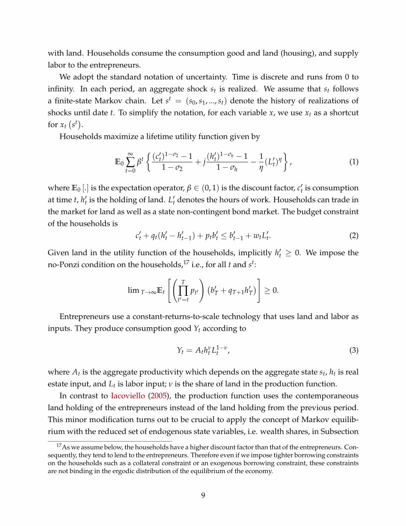
with land. Households consume the consumption good and land (housing), and supplylabor to the entrepreneurs.

We adopt the standard notation of uncertainty. Time is discrete and runs from 0 toinfinity. In each period, an aggregate shock st is realized. We assume that st followsa finite-state Markov chain. Let st = (s0, s1, ..., st) denote the history of realizations ofshocks until date t. To simplify the notation, for each variable x, we use xt as a shortcutfor xt

(st).

Households maximize a lifetime utility function given by

E0

∞

∑t=0

βt{(c′t)

1−σ2 − 11− σ2

+ j(h′t)

1−σh − 11− σh

− 1η(L′t)

η

}, (1)

where E0 [.] is the expectation operator, β ∈ (0, 1) is the discount factor, c′t is consumptionat time t, h′t is the holding of land. L′t denotes the hours of work. Households can trade inthe market for land as well as a state non-contingent bond market. The budget constraintof the households is

c′t + qt(h′t − h′t−1) + ptb′t ≤ b′t−1 + wtL′t. (2)

Given land in the utility function of the households, implicitly h′t ≥ 0. We impose theno-Ponzi condition on the households,17 i.e., for all t and st:

lim T→∞Et

[(T

∏t′=t

pt′

) (b′T + qT+1h′T

)]≥ 0.

Entrepreneurs use a constant-returns-to-scale technology that uses land and labor asinputs. They produce consumption good Yt according to

Yt = Athνt L1−ν

t , (3)

where At is the aggregate productivity which depends on the aggregate state st, ht is realestate input, and Lt is labor input; ν is the share of land in the production function.

In contrast to Iacoviello (2005), the production function uses the contemporaneousland holding of the entrepreneurs instead of the land holding from the previous period.This minor modification turns out to be crucial to apply the concept of Markov equilib-rium with the reduced set of endogenous state variables, i.e. wealth shares, in Subsection

17As we assume below, the households have a higher discount factor than that of the entrepreneurs. Con-sequently, they tend to lend to the entrepreneurs. Therefore even if we impose tighter borrowing constraintson the households such as a collateral constraint or an exogenous borrowing constraint, these constraintsare not binding in the ergodic distribution of the equilibrium of the economy.

9

2.2 and the solution method in Subsection B. However this modification does not affectthe key economic forces in the paper.18

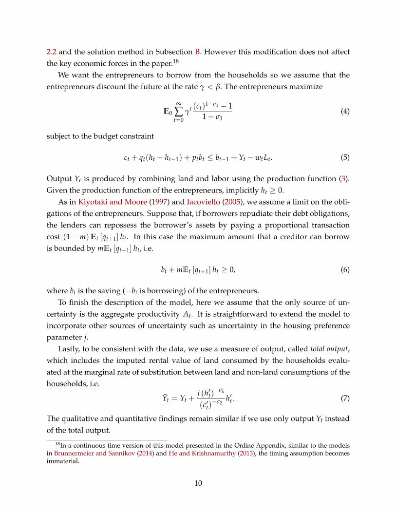
We want the entrepreneurs to borrow from the households so we assume that theentrepreneurs discount the future at the rate γ < β. The entrepreneurs maximize

E0

∞

∑t=0

γt (ct)1−σ1 − 11− σ1

(4)

subject to the budget constraint

ct + qt(ht − ht−1) + ptbt ≤ bt−1 + Yt − wtLt. (5)

Output Yt is produced by combining land and labor using the production function (3).Given the production function of the entrepreneurs, implicitly ht ≥ 0.

As in Kiyotaki and Moore (1997) and Iacoviello (2005), we assume a limit on the obli-gations of the entrepreneurs. Suppose that, if borrowers repudiate their debt obligations,the lenders can repossess the borrower’s assets by paying a proportional transactioncost (1−m)Et [qt+1] ht. In this case the maximum amount that a creditor can borrowis bounded by mEt [qt+1] ht, i.e.

bt + mEt [qt+1] ht ≥ 0, (6)

where bt is the saving (−bt is borrowing) of the entrepreneurs.To finish the description of the model, here we assume that the only source of un-

certainty is the aggregate productivity At. It is straightforward to extend the model toincorporate other sources of uncertainty such as uncertainty in the housing preferenceparameter j.

Lastly, to be consistent with the data, we use a measure of output, called total output,which includes the imputed rental value of land consumed by the households evalu-ated at the marginal rate of substitution between land and non-land consumptions of thehouseholds, i.e.

Yt = Yt +j (h′t)

−σh

(c′t)−σ2

h′t. (7)

The qualitative and quantitative findings remain similar if we use only output Yt insteadof the total output.

18In a continuous time version of this model presented in the Online Appendix, similar to the modelsin Brunnermeier and Sannikov (2014) and He and Krishnamurthy (2013), the timing assumption becomesimmaterial.

10

2.2 Equilibrium

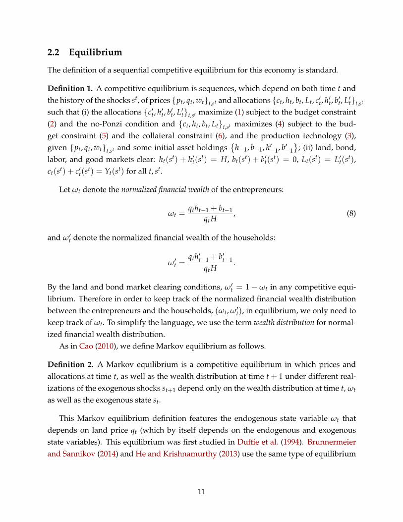
The definition of a sequential competitive equilibrium for this economy is standard.

Definition 1. A competitive equilibrium is sequences, which depend on both time t andthe history of the shocks st, of prices {pt, qt, wt}t,st and allocations {ct, ht, bt, Lt, c′t, h′t, b′t, L′t}t,st

such that (i) the allocations {c′t, h′t, b′t, L′t}t,st maximize (1) subject to the budget constraint(2) and the no-Ponzi condition and {ct, ht, bt, Lt}t,st maximizes (4) subject to the bud-get constraint (5) and the collateral constraint (6), and the production technology (3),given {pt, qt, wt}t,st and some initial asset holdings

{h−1, b−1, h′−1, b′−1

}; (ii) land, bond,

labor, and good markets clear: ht(st) + h′t(st) = H, bt(st) + b′t(s

t) = 0, Lt(st) = L′t(st),

ct(st) + c′t(st) = Yt(st) for all t, st.

Let ωt denote the normalized financial wealth of the entrepreneurs:

ωt =qtht−1 + bt−1

qtH, (8)

and ω′t denote the normalized financial wealth of the households:

ω′t =qth′t−1 + b′t−1

qtH.

By the land and bond market clearing conditions, ω′t = 1− ωt in any competitive equi-librium. Therefore in order to keep track of the normalized financial wealth distributionbetween the entrepreneurs and the households, (ωt, ω′t), in equilibrium, we only need tokeep track of ωt. To simplify the language, we use the term wealth distribution for normal-ized financial wealth distribution.

As in Cao (2010), we define Markov equilibrium as follows.

Definition 2. A Markov equilibrium is a competitive equilibrium in which prices andallocations at time t, as well as the wealth distribution at time t + 1 under different real-izations of the exogenous shocks st+1 depend only on the wealth distribution at time t, ωt

as well as the exogenous state st.

This Markov equilibrium definition features the endogenous state variable ωt thatdepends on land price qt (which by itself depends on the endogenous and exogenousstate variables). This equilibrium was first studied in Duffie et al. (1994). Brunnermeierand Sannikov (2014) and He and Krishnamurthy (2013) use the same type of equilibrium

11

definition in their continuous time models.19 We will use the algorithm developed in Cao(2010) to compute this Markov equilibrium.20

2.3 Solution

In this subsection, we first show the equations that characterize a competitive equilib-rium. A Markov equilibrium is also a competitive equilibrium, therefore it must alsosatisfy these equations.

Given their land holding at time t, ht, the entrepreneurs choose labor demand Lt tomaximize profit

maxLt{Yt − wtLt}

subject to the production technology given in (3). The first order condition (F.O.C.) in Lt

implieswt = (1− ν)Athν

t L−νt , (9)

i.e. Lt =((1−υ)At

wt

) 1ν ht and

Yt − wtLt = πtht

where πt = νAt

((1−ν)At

wt

) 1−νν is profit per unit of land.

Let µt denote the Lagrangian multiplier on the entrepreneurs’ collateral constraint.The F.O.C in the entrepreneurs’ land holding is

(πt − qt)c−σ1t + µtmEt [qt+1] + γEt

[qt+1c−σ1

t+1

]= 0 (10)

and the complementary-slackness condition is

µt (bt + mhtEt [qt+1]) = 0. (11)

19In the Online Appendix, we present a continuous time version of our paper and make this connectionexplicit. However, there are two important differences. First, because of persistent TFP shocks (instead ofI.I.D. depreciation shocks to capital stock as in Brunnermeier and Sannikov (2014) or I.I.D. return shockson dividend as in He and Krishnamurthy (2013)), in our Markov equilibrium, we need to keep track ofboth wealth distribution and the current exogenous shock. Second, we allow for general utility functions,instead of linear or log utility functions as in Brunnermeier and Sannikov (2014) and He and Krishnamurthy(2013).

20We can also define Markov equilibrium using more natural state variables such as ht−1, bt−1, as in mostof the New Keynesian literature using linearization methods, or as in Mendoza (2010) using a nonlinearmethod. Our solution method applies for such concepts of equilibrium as well. However, our currentMarkov equilibrium concept allows us to summarize the dynamic equilibrium in one endogenous statevariable, ωt, which greatly facilitates numerical computations and offers intuitive representations of howwealth distribution affects land price and output in simple graphs.

12

The F.O.C for the entrepreneurs with respect to bond holding is

− ptc−σ1t + µt + γEt

[c−σ1

t+1

]= 0. (12)

Similarly, the F.O.C.s for the households are

h′t : −qtc′−σ2t + jh′−σh

t + βEt

[qt+1c′−σ2

t+1

]= 0 (13)

b′t : −ptc

′−σ2t + βEt

[c′−σ2

t+1

]= 0 (14)

L′t : wtc′−σ2t = L′η−1

t (15)

The first order conditions in ht and h′t shed light on the determinants of land price.Indeed, we can rewrite (10) as

qt = πt + γEt

[qt+1

(ct+1

ct

)−σ1]+ µtmEt [qt+1] cσ1

t .

The first two terms on the right hand side of this equation show that, from the entrepreneurspoint of view, land price is the net present value of present and future profits from pro-duction using land. In addition, the last term on the right hand side shows the collateralvalue of land in the land valuation of the entrepreneurs. Iterating this equation forward,we obtain the expression for land price as the present discounted value of profits, withthe discount factor depending on the marginal utilities of the entrepreneurs as well as onthe multiplier on the collateral constraint:21

qt = πt + Et

[qt+1

{γ

(ct+1

ct

)−σ1

+ µtmcσ1t

}]

= Et

[∞

∑s=0

s−1

∏r=0

{γ

(ct+r+1

ct+r

)−σ1

+ µt+rmcσ1t+r

}πt+s

]. (16)

21This formula is similar to the one in Mendoza (2010). In particular, when the entrepreneurs cannotborrow against their land holding, i.e., m = 0, there will not be any collateral premium in the pricing ofland.

13

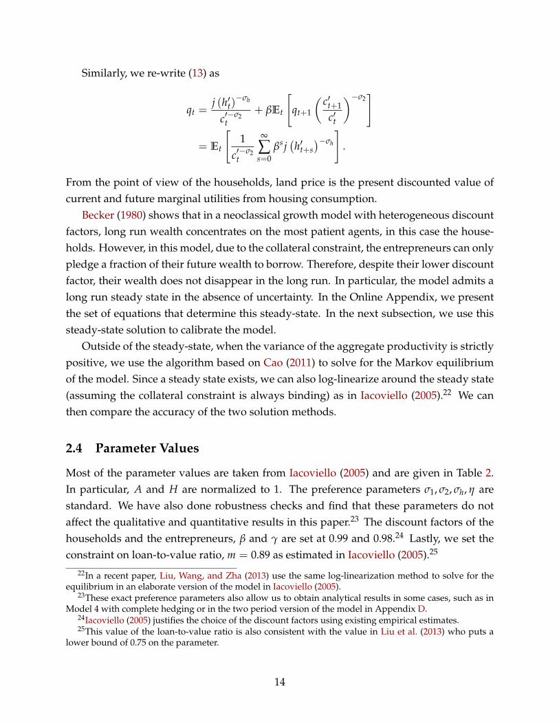
Similarly, we re-write (13) as

qt =j (h′t)

−σh

c′−σ2t

+ βEt

[qt+1

(c′t+1

c′t

)−σ2]

= Et

[1

c′−σ2t

∞

∑s=0

βs j(h′t+s

)−σh

].

From the point of view of the households, land price is the present discounted value ofcurrent and future marginal utilities from housing consumption.

Becker (1980) shows that in a neoclassical growth model with heterogeneous discountfactors, long run wealth concentrates on the most patient agents, in this case the house-holds. However, in this model, due to the collateral constraint, the entrepreneurs can onlypledge a fraction of their future wealth to borrow. Therefore, despite their lower discountfactor, their wealth does not disappear in the long run. In particular, the model admits along run steady state in the absence of uncertainty. In the Online Appendix, we presentthe set of equations that determine this steady-state. In the next subsection, we use thissteady-state solution to calibrate the model.

Outside of the steady-state, when the variance of the aggregate productivity is strictlypositive, we use the algorithm based on Cao (2011) to solve for the Markov equilibriumof the model. Since a steady state exists, we can also log-linearize around the steady state(assuming the collateral constraint is always binding) as in Iacoviello (2005).22 We canthen compare the accuracy of the two solution methods.

2.4 Parameter Values

Most of the parameter values are taken from Iacoviello (2005) and are given in Table 2.In particular, A and H are normalized to 1. The preference parameters σ1, σ2, σh, η arestandard. We have also done robustness checks and find that these parameters do notaffect the qualitative and quantitative results in this paper.23 The discount factors of thehouseholds and the entrepreneurs, β and γ are set at 0.99 and 0.98.24 Lastly, we set theconstraint on loan-to-value ratio, m = 0.89 as estimated in Iacoviello (2005).25

22In a recent paper, Liu, Wang, and Zha (2013) use the same log-linearization method to solve for theequilibrium in an elaborate version of the model in Iacoviello (2005).

23These exact preference parameters also allow us to obtain analytical results in some cases, such as inModel 4 with complete hedging or in the two period version of the model in Appendix D.

24Iacoviello (2005) justifies the choice of the discount factors using existing empirical estimates.25This value of the loan-to-value ratio is also consistent with the value in Liu et al. (2013) who puts a

lower bound of 0.75 on the parameter.

14

Table 2: Baseline Parameter ValuesParameters ValueA 1 mean technologyH 1 total supply of housingβ 0.99 discount factor of householdγ 0.98 discount factor of entrepreneurσ1 1.00 CRRA coefficient of entrepreneurσ2 1.00 CRRA coefficient of householdσh 1.00 CRRA coefficient of household for housingη 1.00 household labor supply elasticitym 0.89 loan-to-value ratio constraint

Table 3: Calibration Targets and Results for j and νParameters Value Target Data

j 0.056 Value of Residential Housing over Total Output 133%ν 0.041 Value of Commercial Housing over Total Output 88%

Two parameters j - households’ weight of housing in utility, and ν - share of land inthe production function are the most important parameters in the model. Housing weightis important since the total output given in equation (7) depends on the marginal utilityfrom housing consumption, and as we show in Online Appendix K, land share in the pro-duction function is a central determinant of the magnitudes of the amplification effects.These two parameters are calibrated using the steady-state equilibrium. We use two mo-ments: the average value of residential real estate over total output and the average valueof commercial real estate over total output from the Flow of Funds to calibrate the twoparameters. We solve for the steady-state of the benchmark model and find (j, ν) suchthat the model’s moments match exactly the empirical moments.26 The empirical valuesof the two moments and the calibrated parameters (j, ν) are presented in Table 3.

In order to use the global nonlinear method described in Appendix B, we need todiscretize the process for At by a finite number of points. For At we use a three pointprocess, At ∈ {A + ∆, A, A− ∆}, which corresponds to expansions, st = G, normal times,st = N, and recessions, st = B.27 We assume the following form of transition matrix

Π =

π 1− π 01−π0

2 π01−π0

2

0 1− π π

. (17)

26We have also verified that the two moments do not change significantly outside of the steady-state.27A two-state process is enough to illustrate the amplification and asymmetric effects, but in order to

match several moments of the productivity process in the U.S. we need at least three states.

15

The exogenous stochastic process of productivity is totally symmetric. However, dueto incomplete markets, the resulting dynamics of the economy become asymmetric asshown in Subsection 2.5 below.

The values of π0 and π are calibrated using historical U.S. data. According to thedefinitions of business cycle expansions and recessions by NBER, there are 12 recessionsin total from post-WWII, January 1945 to December 2013, with an average length of eachrecession of 3.6 quarters. The share of months spent in recessions is 15.7%. Given thetransition matrix Π above, the average length of each recession is 1

1−π so π = 72.04%. π0

is chosen such that the probability of a recession in the stationary distribution for At, i.e.,At = A− ∆ matches the share of months spent in recession which implies π0 = 87.2%.28

As we normalize A to 1, in numerical simulations, we vary ∆ from 1% to 6%, in orderto study the non-linear effects of shocks with different sizes. 29 In the benchmark set ofparameters, we choose an intermediate value for ∆, ∆ = 3%.

2.5 Numerical Results

We apply the nonlinear global solution method for the benchmark model in AppendixB to solve for the dynamic equilibrium of this model. We also solve for the equilib-rium using log-linearization around the steady-state and examine the accuracy of thelog-linearized solution. The equations that determine the log-linearized dynamics arepresented in Online Appendix F. In this subsection, we report the numerical results forthe collateral constraint model with the size of the productivity shock chosen at 3% andother parameters taken from Table 2. The most important properties of the numericalsolutions are the following.

First of all, the global nonlinear solution for Markov equilibrium features an occasion-ally binding collateral constraint. Collateral constraint (6) binds when the entrepreneurs’wealth is sufficiently low. In this binding region, endogenous variables including landprice and output are more sensitive to changes in wealth distribution. Second, the equi-librium is asymmetric with respect to bad shocks versus good shocks despite the fact that

28From the transition matrix for At, the probability of recession in the stationary distribution is1−π0

2(2−π−π0).

29Given the exogenous process for productivity, the standard deviation of productivity is given by√1−π0

2−π−π0∆. From our own estimates using quarterly TFP data from St Louis Fed (see empirical appendix

E), ∆ is approximately 1.8%. This low value of ∆ is consistent with the the estimates from Liu, Wang, andZha (2013), which yield ∆ slightly lower than 1%. However, to generate the annual standard deviation ofproductivity in the U.S. economy of about 15% in Khan and Thomas (2013), ∆ is approximately 6%. Giventhe wide range of the possible values of ∆, we choose ∆ = 3% at the middle of the range. In OnlineAppendix I, we examine other values of ∆ in the range.

16

the stochastic structure of the shocks is totally symmetric. Third, when the collateral con-straint binds, the responses of land price and output amplify negative technology shocks.

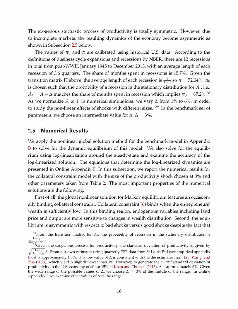
Figure 1 shows the policy functions (consumption of the entrepreneurs and the house-holds and the total output) and the pricing function for land conditional on the exogenousstate st and the endogenous state ωt , in expansions (st = G, solid blue lines), normaltimes (st = N, purple dash-dotted lines) and recessions (st = B, dashed red lines). Eventhough the global nonlinear method solves for the policy and pricing functions for thewhole range of ωt, Figure 1 is restricted to the values of ωt in the support of the stationarydistribution of ωt. Because of the collateral constraint, the functions exhibit significantlymore nonlinearity when ωt is close to zero where the collateral constraint is binding.When the collateral constraint binds, the standard feed-back effect in Kiyotaki and Moore(1997) kicks in: after a negative productivity shock, even temporary, the entrepreneurshave to cut back their land holding, ht, in order to smooth consumption; they cannotborrow more due to the collateral constraint. This reduction in land demand depressesland price, qt, which through the collateral constraint, forces the entrepreneurs to reducetheir debt, partly by reducing consumption, and further cut back their land holding. Thisvicious cycle results in a significant decline in land price, as well as in the entrepreneurs’land holding and the total output. There is also an inter-temporal feedback: lower currentwealth of the entrepreneurs leads to lower future wealth and lower future land prices.Given that the current land price is a weighted average of current per unit profit and fu-ture land price, as shown in the asset pricing equations, lower future land price in turnleads to lower current land price. The entrepreneurs use land to produce; so a significantdecrease in land holding leads to a significant decrease in output.

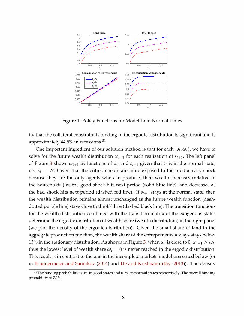
The advantage of the nonlinear solution method used in this paper is that, we can seeclearly two regions of the state space in which the economy follows different dynamics.In one region, when the collateral constraint is binding (or nearly binding), the feed-backeffect is important. In the other region when the collateral constraint is far from binding,asset price and output are less sensitive to changes in the wealth distribution.30 Figure 2helps us determine the neighborhood of wealth distribution in which the collateral con-straint starts to bind. The upper panel shows the portfolio choice of the entrepreneurs asa function of ωt and st = N. On the left of the vertical green line (in both panels), aroundωt = 0.05, the collateral constraint is close to be binding and will bind if st+1 = B. Thelower panel shows the ergodic distribution of ωt conditional on st = N. The probabil-

30We can also see different dynamics between the two regions by looking at dxtdωt

, x = q, Y, as functions ofωt, i.e. the marginal effect of redistributing wealth from the households to the entrepreneurs on land priceand output. Figure 1 suggests that these functions are decreasing in ωt and are much higher at lower ωtwhen the collateral constraint is binding.

17

ωt

0.05 0.1 0.157.6

7.8

8

8.2

8.4

8.6

8.8

9

9.2Land Price

ωt

0.05 0.1 0.150.9

0.95

1

1.05Total Output

ωt

0.05 0.1 0.150

0.005

0.01

0.015

0.02

0.025

0.03

0.035Consumption of Entrepreneurs

st=G

st=N

st=B

ωt

0.05 0.1 0.150.84

0.86

0.88

0.9

0.92

0.94

0.96Consumption of Households

Figure 1: Policy Functions for Model 1a in Normal Times

ity that the collateral constraint is binding in the ergodic distribution is significant and isapproximately 44.5% in recessions.31

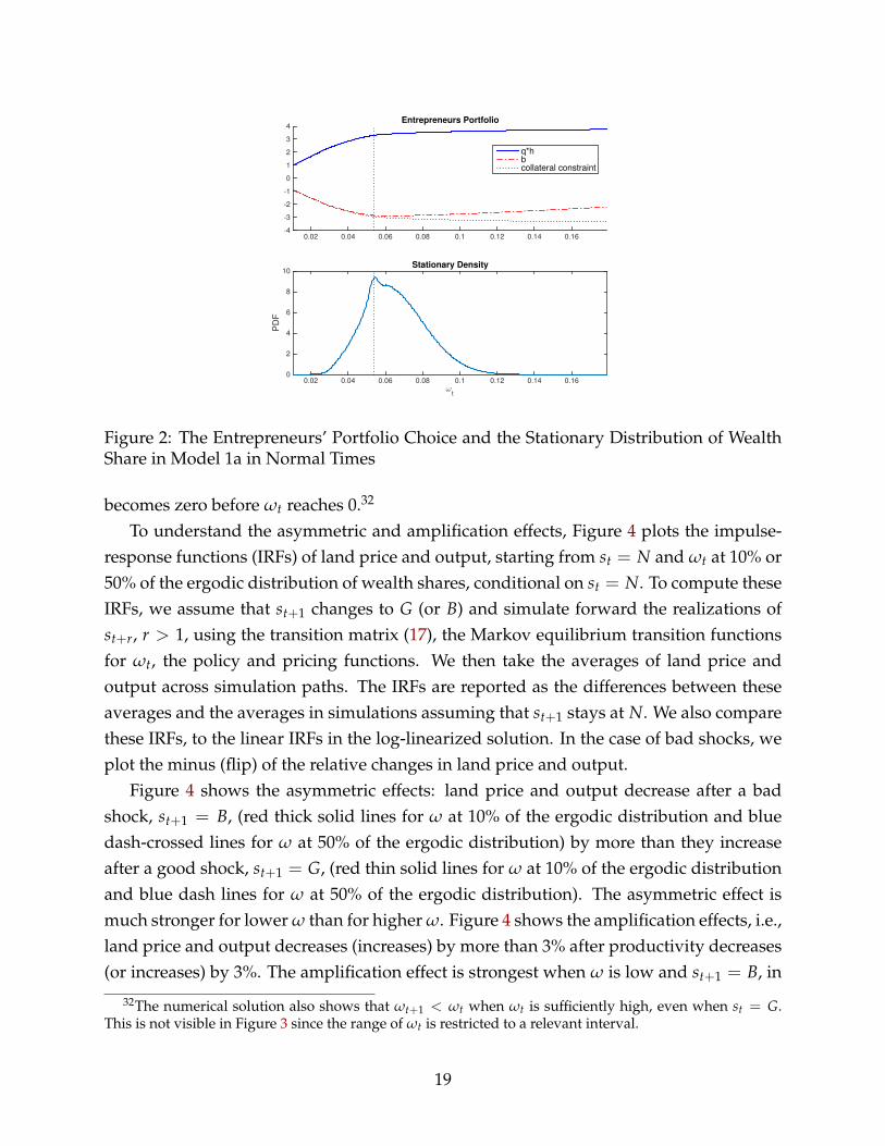
One important ingredient of our solution method is that for each (st, ωt), we have tosolve for the future wealth distribution ωt+1 for each realization of st+1. The left panelof Figure 3 shows ωt+1 as functions of ωt and st+1 given that st is in the normal state,i.e. st = N. Given that the entrepreneurs are more exposed to the productivity shockbecause they are the only agents who can produce, their wealth increases (relative tothe households’) as the good shock hits next period (solid blue line), and decreases asthe bad shock hits next period (dashed red line). If st+1 stays at the normal state, thenthe wealth distribution remains almost unchanged as the future wealth function (dash-dotted purple line) stays close to the 45o line (dashed black line). The transition functionsfor the wealth distribution combined with the transition matrix of the exogenous statesdetermine the ergodic distribution of wealth share (wealth distribution) in the right panel(we plot the density of the ergodic distribution). Given the small share of land in theaggregate production function, the wealth share of the entrepreneurs always stays below15% in the stationary distribution. As shown in Figure 3, when ωt is close to 0, ωt+1 > ωt,thus the lowest level of wealth share ωt = 0 is never reached in the ergodic distribution.This result is in contrast to the one in the incomplete markets model presented below (orin Brunnermeier and Sannikov (2014) and He and Krishnamurthy (2013)). The density

31The binding probability is 0% in good states and 0.2% in normal states respectively. The overall bindingprobability is 7.1%.

18

0.02 0.04 0.06 0.08 0.1 0.12 0.14 0.16-4

-3

-2

-1

0

1

2

3

4Entrepreneurs Portfolio

q*hbcollateral constraint

ωt

0.02 0.04 0.06 0.08 0.1 0.12 0.14 0.16

PD

F

0

2

4

6

8

10Stationary Density

Figure 2: The Entrepreneurs’ Portfolio Choice and the Stationary Distribution of WealthShare in Model 1a in Normal Times

becomes zero before ωt reaches 0.32

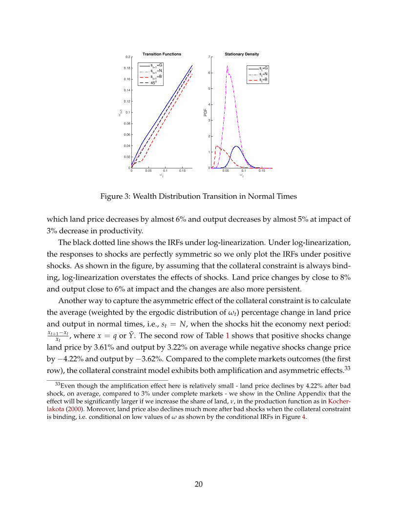
To understand the asymmetric and amplification effects, Figure 4 plots the impulse-response functions (IRFs) of land price and output, starting from st = N and ωt at 10% or50% of the ergodic distribution of wealth shares, conditional on st = N. To compute theseIRFs, we assume that st+1 changes to G (or B) and simulate forward the realizations ofst+r, r > 1, using the transition matrix (17), the Markov equilibrium transition functionsfor ωt, the policy and pricing functions. We then take the averages of land price andoutput across simulation paths. The IRFs are reported as the differences between theseaverages and the averages in simulations assuming that st+1 stays at N. We also comparethese IRFs, to the linear IRFs in the log-linearized solution. In the case of bad shocks, weplot the minus (flip) of the relative changes in land price and output.

Figure 4 shows the asymmetric effects: land price and output decrease after a badshock, st+1 = B, (red thick solid lines for ω at 10% of the ergodic distribution and bluedash-crossed lines for ω at 50% of the ergodic distribution) by more than they increaseafter a good shock, st+1 = G, (red thin solid lines for ω at 10% of the ergodic distributionand blue dash lines for ω at 50% of the ergodic distribution). The asymmetric effect ismuch stronger for lower ω than for higher ω. Figure 4 shows the amplification effects, i.e.,land price and output decreases (increases) by more than 3% after productivity decreases(or increases) by 3%. The amplification effect is strongest when ω is low and st+1 = B, in

32The numerical solution also shows that ωt+1 < ωt when ωt is sufficiently high, even when st = G.This is not visible in Figure 3 since the range of ωt is restricted to a relevant interval.

19

ωt

0 0.05 0.1 0.15

ωt+

1

0

0.02

0.04

0.06

0.08

0.1

0.12

0.14

0.16

0.18

0.2Transition Functions

st+1

=G

st+1

=N

st+1

=B

45o

ωt

0.05 0.1 0.15

PD

F

0

1

2

3

4

5

6

7Stationary Density

st=G

st=N

st=B

Figure 3: Wealth Distribution Transition in Normal Times

which land price decreases by almost 6% and output decreases by almost 5% at impact of3% decrease in productivity.

The black dotted line shows the IRFs under log-linearization. Under log-linearization,the responses to shocks are perfectly symmetric so we only plot the IRFs under positiveshocks. As shown in the figure, by assuming that the collateral constraint is always bind-ing, log-linearization overstates the effects of shocks. Land price changes by close to 8%and output close to 6% at impact and the changes are also more persistent.

Another way to capture the asymmetric effect of the collateral constraint is to calculatethe average (weighted by the ergodic distribution of ωt) percentage change in land priceand output in normal times, i.e., st = N, when the shocks hit the economy next period:xt+1−xt

xt, where x = q or Y. The second row of Table 1 shows that positive shocks change

land price by 3.61% and output by 3.22% on average while negative shocks change priceby−4.22% and output by−3.62%. Compared to the complete markets outcomes (the firstrow), the collateral constraint model exhibits both amplification and asymmetric effects.33

33Even though the amplification effect here is relatively small - land price declines by 4.22% after badshock, on average, compared to 3% under complete markets - we show in the Online Appendix that theeffect will be significantly larger if we increase the share of land, ν, in the production function as in Kocher-lakota (2000). Moreover, land price also declines much more after bad shocks when the collateral constraintis binding, i.e. conditional on low values of ω as shown by the conditional IRFs in Figure 4.

20

t0 5 10 15 20 25 30

%

0

1

2

3

4

5

6

7

8Percentage Deviation of Land Price after 3% shocks

dynamics (flipped) after B shock, ω at 10%dynamics after G shock, ω at 10%dynamics (flipped) after B shock, ω at 50%dynamics after G shock, ω at 50%loglinearized result

t0 5 10 15 20 25 30

%

0

1

2

3

4

5

6Percentage Deviation of Total Output after 3% shocks

dynamics (flipped) after B shock, ω at 10%dynamics after G shock, ω at 10%dynamics (flipped) after B shock, ω at 50%dynamics after G shock, ω at 50%loglinearized result

Figure 4: IRFs for Non-Linear versus Log-Linear Model

2.6 Alternative Collateral Constraints

In the collateral constraint (6), we use the expected future land price. This constraintcan be micro-founded under limited commitment and has been used in a large numberof papers including Kiyotaki and Moore (1997), Iacoviello (2005), Fostel and Geanako-plos (2008), Geanakoplos (2010), and Cao (2011).34 However, in practice collateralizedcontracts are often written using current asset prices and this is also assumed in a largenumber of papers, for example Mendoza (2010). Figure 3 shows that the wealth distribu-tion, ωt, moves very slowly over the business cycles, and as a result land price also movesslowly. Therefore using current or expected future land price should not imply quantita-tively significant differences between the two models. We can show this result rigorouslyby solving an alternative model in which the collateral constraint (6) is replaced by thefollowing alternative collateral constraint:

bt + mqtht ≥ 0.

Fortunately this case is a special case of the general Markov equilibrium definition and

34Cao (2011) shows that when the lender can seize a fraction of the asset upon default, the collateralconstraint arises endogenously and has the form

bt(st) + mht minst+1|st

qt+1

(st+1

)≥ 0.

If we use this collateral constraint the average responses of land price and output after 3% negative shocksare -3.98% and -3.38% respectively.

21

the solution method in Cao (2010). We solve for the Markov equilibrium under this alter-native collateral constraint for the same parameters used in Subsection 3.1. The solutionis quantitatively similar to the solution of the collateral constraint model in Subsection3.1. For example, Row 3 in Table 1 shows that the amplification and asymmetric effectsare only slightly higher than the ones in Subsection 3.1 (Row 2).

3 Incomplete Markets Model

The benchmark model with incomplete markets and collateral constraint delivers ampli-fied and asymmetric responses of the economy to exogenous shocks. To understand theimportance of market incompleteness versus collateral constraint for the amplificationand asymmetric effects, in this section, we study a model in which markets are incom-plete, i.e. the entrepreneurs can only borrow by issuing state non-contingent bonds, butthey do not face a collateral constraint. Instead, we impose only the no-Ponzi conditionon the entrepreneurs, i.e., for all t and st,

lim T→∞Et

[(T

∏t′=t

pt′

)(bT + qT+1hT)

]≥ 0.

We call this model Model 2. The definitions of the competitive equilibrium and Markovequilibrium are similar to those in the benchmark model, Model 1a, with incompletemarkets and a collateral constraint.

The first-order conditions (F.O.C.s) in ht and bt in the maximization problem of theentrepreneurs imply

(πt − qt)c−σ1t + γEt[qt+1c−σ1

t+1 ] = 0 (18)

and− ptc

−σ1t + γEt

[c−σ1

t+1

]= 0. (19)

We rewrite (18) as

qt = πt + γEt

[qt+1

(ct+1

ct

)−σ1]

= Et

[∞

∑s=0

γs(

ct+s

ct

)−σ1

πt+s

].

The right hand side of this equation shows that, from the entrepreneurs’ point of view,

22

land price is the net present discounted value of present and future profits from pro-duction using land and the discount factor depends on the marginal utility of the en-trepreneurs. Notice that compared to the pricing equation, (16), land no longer has col-lateral values to the entrepreneurs.

Despite the fact that we do not impose any constraint on the entrepreneurs’ borrowingexcept for the no-Ponzi schemes condition, the following lemma shows that, in equilib-rium, the financial wealth of the entrepreneurs is endogenously bounded from below by0.

Lemma 1. In any competitive equilibrium, thus any Markov equilibrium, we must have ωt ≥ 0for all t and st.

Proof. Appendix C.

One consequence of this lemma is that the competitive, or Markov equilibrium willnot change if we replace the no-Ponzi schemes condition on the entrepreneurs by a morestringent borrowing constraint

ωt+1(st+1) = bt(st) + qt+1(st+1)ht(st) ≥ 0

for all t, st. When 0 < σ1 ≤ 1, we also show that this is the natural borrowing limit, i.e. inequilibrium, any feasible plan - plan that implies positive consumption at all times and inall states - must satisfy the inequality ωt ≥ 0 for all t and st.

3.1 Numerical Results

In this subsection, we present the numerical results for the incomplete markets model -Model 2 - with the parameters in Subsection 2.4.

Quantitatively, Row 4 in Table 1 shows the average (over the ergodic distribution ofωt) of the changes in land price and total output given the current normal state, st = N.We observe significant amplification and asymmetric effects under incomplete markets.By comparing the amplification effects in this model (Row 4 in Table 1) to the amplifi-cation effects in the benchmark model (Row 2 in Table 1) - Model 1a with both marketincompleteness and collateral constraints - we can say that market incompleteness ac-counts for about two thirds of the amplification effects.35

35For example, after a 3% negative TFP shock, on average, output decreases by -3.40% with marketincompleteness alone compared to -3.62% in the model with market incompleteness and collateral con-straints. As a result, about 64% ( 3.40%−3%

3.62%−3% ) of the amplification in output is accounted for by market in-completeness. Similarly, about 66% ( 3.81%−3%

4.22%−3% ) of the amplification in land price is accounted for by marketincompleteness.

23

Under market incompleteness only, the amplification and asymmetric responses comefrom the net worth effect as follows. An initial negative shock decreases land productivityand consequently land price. Because of market incompleteness, the value of debt ofthe entrepreneurs, which is determined from the previous period, is independent of theshock. Therefore, the decrease in land price leads to a decrease in the net worth of theentrepreneurs, which reduces their demand for land. Because only the entrepreneurscan use land to produce, the reduction in their land demand further depresses the priceof land, which further lowers their net worth, setting off the vicious cycle of falling landprice and falling net worth. Thus the effects of a negative productivity shock on land priceand production are amplified. Moreover, because the production and utility functionsare concave, a negative productivity shock has larger effect than a positive productivityshock through the net worth channel. In Appendix D, we study a two-period version ofour model with log utilities to derive analytically the net worth effect.36

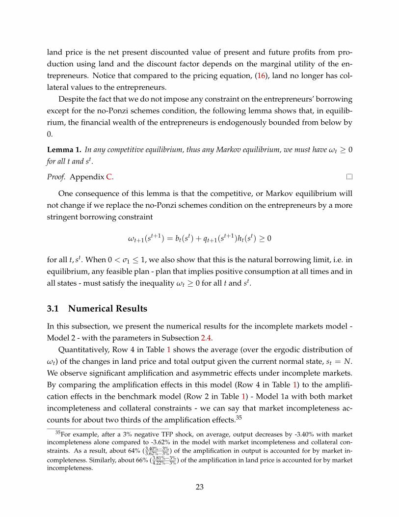
Figure 5 shows the policy functions (consumptions of the entrepreneurs and the house-holds and total output) and the pricing function for land conditional on the exogenousstate st = B and the endogenous state ωt (blue solid lines - for comparison, the dashedred lines are the functions in Model 1a). Figure 5 is restricted to the values of ωt in thesupport of the ergodic distribution. We observe that, despite the absence of a collateralconstraint, land price and output functions are nonlinear in the wealth distribution. Inparticular they are more sensitive to changes in the wealth distribution when the wealthof the entrepreneurs is low.37

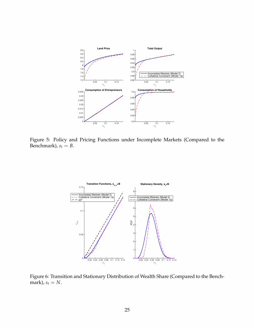
Figure 6 is the counterpart of Figure 3 for Model 1a, showing the transition function(left panel) and the stationary distribution (right panel) when s = N compared to the onesin Model 1a. Nonlinearity implies asymmetric responses of the equilibrium land priceand output with respect to productivity shocks. Starting from st = N, the good shock,i.e., st+1 = G increases the entrepreneurs’ wealth and the bad shock st+1 = B decreasesthe entrepreneurs’ wealth, as shown in Figure 6. But conditional on the same change inentrepreneurs’ wealth, land price and output increase after a good shock by less than theydecrease after a bad shock due to nonlinearity. This leads to the asymmetric responses ofequilibrium land price and output to symmetric shocks, as shown quantitatively in Table1.

Despite the amplification and asymmetric effects in Model 2 due to the net worth effect

36We also show that, under complete markets, this effect disappears because the entrepreneurs can per-fectly insure their net worth against productivity shocks.

37Similar to the observation in footnote 30, another way to see the nonlinearity is to look at dxtdωt

, x = qor Y, as functions of ωt. Figure 5 suggests that these functions are decreasing in ωt and are much higher atlower ωt.

24

ωt

0.05 0.1 0.157.2

7.4

7.6

7.8

8

8.2

8.4

8.6

8.8Land Price

ωt

0.05 0.1 0.150.86

0.88

0.9

0.92

0.94

0.96

0.98

1Total Output

Incomplete Markets (Model 2)Collateral Constraint (Model 1a)

ωt

0.05 0.1 0.150

0.005

0.01

0.015

0.02

0.025

0.03

0.035Consumption of Entrepreneurs

ωt

0.05 0.1 0.150.8

0.82

0.84

0.86

0.88

0.9Consumption of Households

Figure 5: Policy and Pricing Functions under Incomplete Markets (Compared to theBenchmark), st = B.

ωt

0.02 0.04 0.06 0.08 0.1 0.12 0.14

ωt+

1

0

0.05

0.1

0.15

Transition Functions, st+1

=B

Incomplete Markets (Model 2)Collateral Constraint (Model 1a)45

o

ωt

0.02 0.04 0.06 0.08 0.1 0.12 0.14

PD

F

0

1

2

3

4

5

6

7

8

Stationary Density, st=N

Incomplete Markets (Model 2)Collateral Constraint (Model 1a)

Figure 6: Transition and Stationary Distribution of Wealth Share (Compared to the Bench-mark), st = N.

25

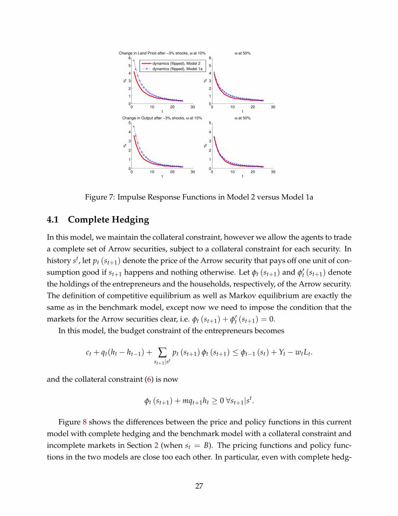
coming from market incompleteness, a collateral constraint, in addition to market incom-pleteness, does amplify exogenous shocks more, especially when the collateral constraintbinds. This can be seen from the more nonlinearity of the policy and pricing functionsfor Model 1a compared to Model 2 in Figure 5 when ω is low. It can also be seen moreclearly from the conditional IRFs (as defined in Subsection 2.5) depicted in Figure 7. Thethick red lines are the IRFs in Model 2 and the crossed blue lines are the IRFs in Model 1a.To simplify the figure, we only plot the IRFs after a negative shock. The left panels showthe (flipped) impulse responses of land price and output after a −3% productivity shock,conditional on st = N and ωt at the 10th percentile of the ergodic distribution in eachmodel. Similarly, the right panel shows the impulse responses conditional on st = N andωt at the 50th percentile. The figure shows that when ωt is high the responses are similarin both models. However, when ωt is low the responses are significantly larger in Model1a with collateral constraint.

Then, why is it the case that Model 2 without the collateral constraint accounts forclose to two thirds of the average amplification effect in Model 1a? The answer lies inthe transition functions and stationary distributions depicted in Figure 6. The left panelshows that due to precautionary saving, in Model 1a, the entrepreneurs refrain from bor-rowing too much, compared to the amount of borrowing in Model 2, to avoid a bindingcollateral constraint. Consequently, as depicted in the right panel, the ergodic distributionof wealth shares in Model 1a has less mass at lower levels of ω compared to the ergodicdistribution in Model 2. This difference attenuates the significant amplification effect atlow ω’s (when the collateral constraint binds) in Model 1a. This intuition also suggeststhat in models with larger amplification effects due to a collateral constraint, the precau-tionary saving channel is stronger and the collateral constraint binds less often. Thereforemarket incompleteness will account for more of the amplification in these models. Weconfirm this intuition in Online Appendix K.

4 Hedging with Collateral Constraints

The comparison between the benchmark model - Model 1a - in Section 2 and the incom-plete markets model - Model 2 - in Section 3 suggests that one of the main ingredients forthe amplification and asymmetric effects is market incompleteness beside the collateralconstraint. To further demonstrate this point, we study two variations of the benchmarkmodel, which we call the complete hedging model (Model 3) and partial hedging model(Model 4).

26

0 10 20 300

1

2

3

4

5

6

t

%

Change in Land Price after −3% shocks, ω at 10%

dynamics (flipped), Model 2

dynamics (flipped), Model 1a

0 10 20 300

1

2

3

4

5

t

%

Change in Output after −3% shocks, ω at 10%

0 10 20 300

1

2

3

4

5

6

t

%

ω at 50%

0 10 20 300

1

2

3

4

5

t

%

ω at 50%

Figure 7: Impulse Response Functions in Model 2 versus Model 1a

4.1 Complete Hedging

In this model, we maintain the collateral constraint, however we allow the agents to tradea complete set of Arrow securities, subject to a collateral constraint for each security. Inhistory st, let pt (st+1) denote the price of the Arrow security that pays off one unit of con-sumption good if st+1 happens and nothing otherwise. Let φt (st+1) and φ′t (st+1) denotethe holdings of the entrepreneurs and the households, respectively, of the Arrow security.The definition of competitive equilibrium as well as Markov equilibrium are exactly thesame as in the benchmark model, except now we need to impose the condition that themarkets for the Arrow securities clear, i.e. φt (st+1) + φ′t (st+1) = 0.

In this model, the budget constraint of the entrepreneurs becomes

ct + qt(ht − ht−1) + ∑st+1|st

pt (st+1) φt (st+1) ≤ φt−1 (st) + Yt − wtLt.

and the collateral constraint (6) is now

φt (st+1) + mqt+1ht ≥ 0 ∀st+1|st.

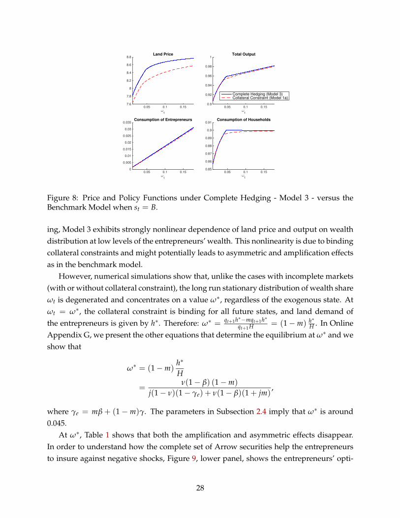
Figure 8 shows the differences between the price and policy functions in this currentmodel with complete hedging and the benchmark model with a collateral constraint andincomplete markets in Section 2 (when st = B). The pricing functions and policy func-tions in the two models are close too each other. In particular, even with complete hedg-

27

ωt

0.05 0.1 0.157.6

7.8

8

8.2

8.4

8.6

8.8Land Price

ωt

0.05 0.1 0.150.9

0.92

0.94

0.96

0.98

1Total Output

Complete Hedging (Model 3)Collateral Constraint (Model 1a)

ωt

0.05 0.1 0.150

0.005

0.01

0.015

0.02

0.025

0.03

0.035Consumption of Entrepreneurs

ωt

0.05 0.1 0.150.85

0.86

0.87

0.88

0.89

0.9

0.91Consumption of Households

Figure 8: Price and Policy Functions under Complete Hedging - Model 3 - versus theBenchmark Model when st = B.

ing, Model 3 exhibits strongly nonlinear dependence of land price and output on wealthdistribution at low levels of the entrepreneurs’ wealth. This nonlinearity is due to bindingcollateral constraints and might potentially leads to asymmetric and amplification effectsas in the benchmark model.

However, numerical simulations show that, unlike the cases with incomplete markets(with or without collateral constraint), the long run stationary distribution of wealth shareωt is degenerated and concentrates on a value ω∗, regardless of the exogenous state. Atωt = ω∗, the collateral constraint is binding for all future states, and land demand ofthe entrepreneurs is given by h∗. Therefore: ω∗ = qt+1h∗−mqt+1h∗

qt+1H = (1−m) h∗H . In Online

Appendix G, we present the other equations that determine the equilibrium at ω∗ and weshow that

ω∗ = (1−m)h∗

H

=ν(1− β) (1−m)

j(1− ν)(1− γe) + ν(1− β)(1 + jm),

where γe = mβ + (1− m)γ. The parameters in Subsection 2.4 imply that ω∗ is around0.045.

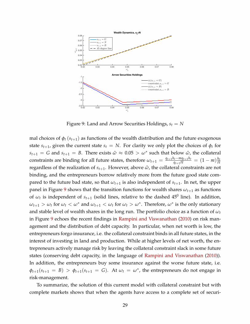
At ω∗, Table 1 shows that both the amplification and asymmetric effects disappear.In order to understand how the complete set of Arrow securities help the entrepreneursto insure against negative shocks, Figure 9, lower panel, shows the entrepreneurs’ opti-

28

ωt

0.02 0.03 0.04 0.05 0.06 0.07 0.08

ωt+

1

0.02

0.03

0.04

0.05

0.06

0.07

0.08

Wealth Dynamics, st=N

st+1 = G

st+1 = N

st+1 = B

45 degree line

ωt

0.02 0.03 0.04 0.05 0.06 0.07 0.08-3.5

-3

-2.5

-2

-1.5

-1Arrow Securities Holdings

φt(st+1 = G)constraint,st+1 = G

φt(st+1 = B)constraint,st+1 = B

Figure 9: Land and Arrow Securities Holdings, st = N

mal choices of φt (st+1) as functions of the wealth distribution and the future exogenousstate st+1, given the current state st = N. For clarity we only plot the choices of φt forst+1 = G and st+1 = B. There exists ω ≈ 0.05 > ω∗ such that below ω, the collateralconstraints are binding for all future states, therefore ωt+1 = qt+1ht−mqt+1ht

qt+1H = (1− m) htH

regardless of the realization of st+1. However, above ω, the collateral constraints are notbinding, and the entrepreneurs borrow relatively more from the future good state com-pared to the future bad state, so that ωt+1 is also independent of st+1. In net, the upperpanel in Figure 9 shows that the transition functions for wealth shares ωt+1 as functionsof ωt is independent of st+1 (solid lines, relative to the dashed 450 line). In addition,ωt+1 > ωt for ωt < ω∗ and ωt+1 < ωt for ωt > ω∗. Therefore, ω∗ is the only stationaryand stable level of wealth shares in the long run. The portfolio choice as a function of ωt

in Figure 9 echoes the recent findings in Rampini and Viswanathan (2010) on risk man-agement and the distribution of debt capacity. In particular, when net worth is low, theentrepreneurs forgo insurance, i.e. the collateral constraint binds in all future states, in theinterest of investing in land and production. While at higher levels of net worth, the en-trepreneurs actively manage risk by leaving the collateral constraint slack in some futurestates (conserving debt capacity, in the language of Rampini and Viswanathan (2010)).In addition, the entrepreneurs buy some insurance against the worse future state, i.e.φt+1(st+1 = B) > φt+1(st+1 = G). At ωt = ω∗, the entrepreneurs do not engage inrisk-management.

To summarize, the solution of this current model with collateral constraint but withcomplete markets shows that when the agents have access to a complete set of securi-

29

ties, amplification and asymmetric effects disappear.38 This point is also made by Krish-namurthy (2003) in a simple 3-period economy and DiTella (2014) in a continuous-timemodel.39

4.2 Partial Hedging

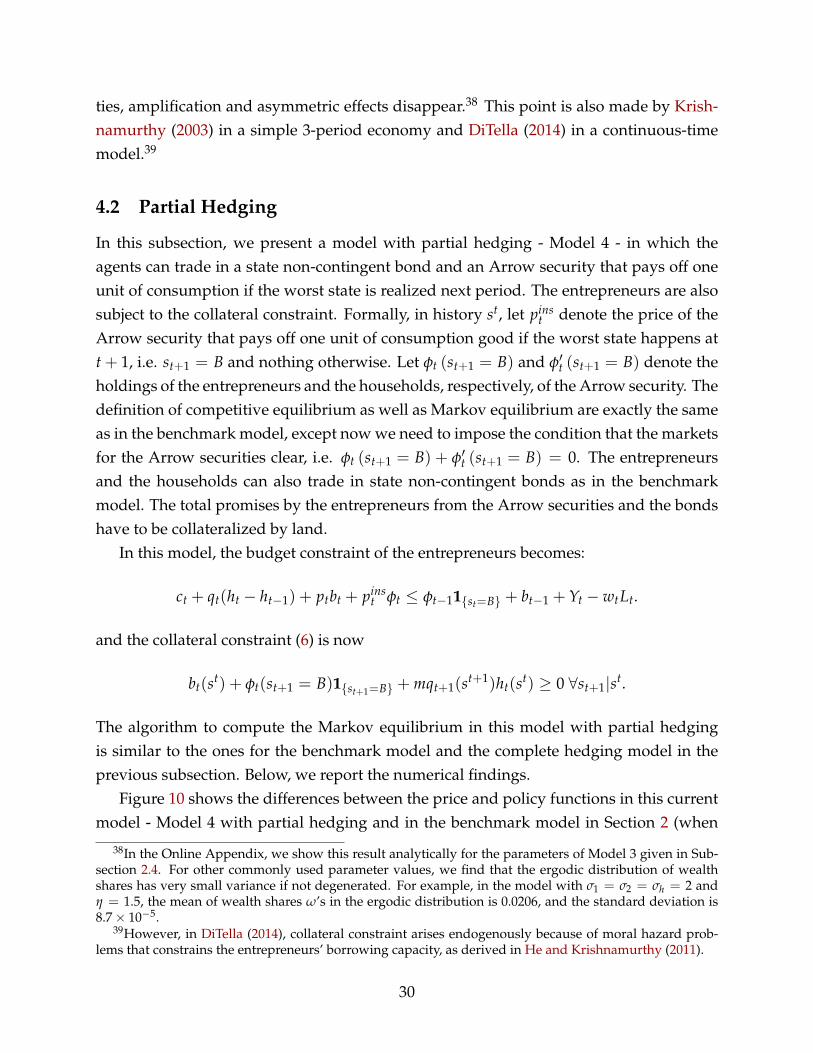
In this subsection, we present a model with partial hedging - Model 4 - in which theagents can trade in a state non-contingent bond and an Arrow security that pays off oneunit of consumption if the worst state is realized next period. The entrepreneurs are alsosubject to the collateral constraint. Formally, in history st, let pins

t denote the price of theArrow security that pays off one unit of consumption good if the worst state happens att + 1, i.e. st+1 = B and nothing otherwise. Let φt (st+1 = B) and φ′t (st+1 = B) denote theholdings of the entrepreneurs and the households, respectively, of the Arrow security. Thedefinition of competitive equilibrium as well as Markov equilibrium are exactly the sameas in the benchmark model, except now we need to impose the condition that the marketsfor the Arrow securities clear, i.e. φt (st+1 = B) + φ′t (st+1 = B) = 0. The entrepreneursand the households can also trade in state non-contingent bonds as in the benchmarkmodel. The total promises by the entrepreneurs from the Arrow securities and the bondshave to be collateralized by land.

In this model, the budget constraint of the entrepreneurs becomes:

ct + qt(ht − ht−1) + ptbt + pinst φt ≤ φt−11{st=B} + bt−1 + Yt − wtLt.

and the collateral constraint (6) is now

bt(st) + φt(st+1 = B)1{st+1=B} + mqt+1(st+1)ht(st) ≥ 0 ∀st+1|st.

The algorithm to compute the Markov equilibrium in this model with partial hedgingis similar to the ones for the benchmark model and the complete hedging model in theprevious subsection. Below, we report the numerical findings.

Figure 10 shows the differences between the price and policy functions in this currentmodel - Model 4 with partial hedging and in the benchmark model in Section 2 (when

38In the Online Appendix, we show this result analytically for the parameters of Model 3 given in Sub-section 2.4. For other commonly used parameter values, we find that the ergodic distribution of wealthshares has very small variance if not degenerated. For example, in the model with σ1 = σ2 = σh = 2 andη = 1.5, the mean of wealth shares ω’s in the ergodic distribution is 0.0206, and the standard deviation is8.7× 10−5.

39However, in DiTella (2014), collateral constraint arises endogenously because of moral hazard prob-lems that constrains the entrepreneurs’ borrowing capacity, as derived in He and Krishnamurthy (2011).

30

0.05 0.1 0.157.5

8

8.5

9

Land Price

ωt

0.05 0.1 0.150.9

0.95

1

Total Output

ωt

Partial Hedging (Model 4)

Collateral Constraint (Model 1a)

0.05 0.1 0.150

0.01

0.02

0.03

0.04

Consumption of Entrepreneurs

ωt

0.05 0.1 0.150.84

0.86

0.88

0.9

0.92

Consumption of Households

ωt

Figure 10: Price and Policy Functions under Partial Hedging - Model 4 - Compared to theBenchmark Model, st = B.

st = B). Figure 11 shows the differences between the transition functions and the sta-tionary distributions between the two models. We observe that even though both modelsfeature highly nonlinear price and policy functions for lower values of wealth, in Model4 with partial hedging, the entrepreneurs are able to insure themselves against the worseshocks. Therefore, the stationary distribution has much lower masses at lower valuesof wealth compared to the benchmark model. Consequently, Table 1 shows that the av-erage amplification effect is much smaller, virtually absent for st = B, compared to thebenchmark model.

5 Some Empirical Evidence

The results from our model show that productivity (TFP) shocks have asymmetric effectson the output and land prices. First, negative TFP shocks have larger effects than pos-itive TFP shocks as indicated in Table 1. Second, the effects also depend on the wealthdistribution: they are larger when the wealth share of the entrepreneurs is low. Lastly,combining the previous two points, the responses should be the strongest when we haveboth low TFP shocks and low wealth share of the entrepreneurs. We offer some empir-ical evidence of these implications in this section.40 In particular, we use four quarterly

40Following Liu, Wang, and Zha (2013), we interpret the entrepreneurs in the model as the non-financialbusiness sector in the data.

31

ωt

0.02 0.04 0.06 0.08 0.1 0.12 0.14

ωt+

1

0

0.02

0.04

0.06

0.08

0.1

0.12

0.14

Transition Functions, st+1

=B

Partial Hedging (Model 4)Collateral Constraint (Model 1a)

45o

ωt

0.02 0.04 0.06 0.08 0.1 0.12 0.14

PD

F

0

5

10

15

20

25

30

Stationary Density, st=N

Partial Hedging (Model 4)Collateral Constraint (Model 1a)

Figure 11: Transition and Stationary Distribution of Wealth Share under Partial Hedging- Compared to the Benchmark Model, st = N.

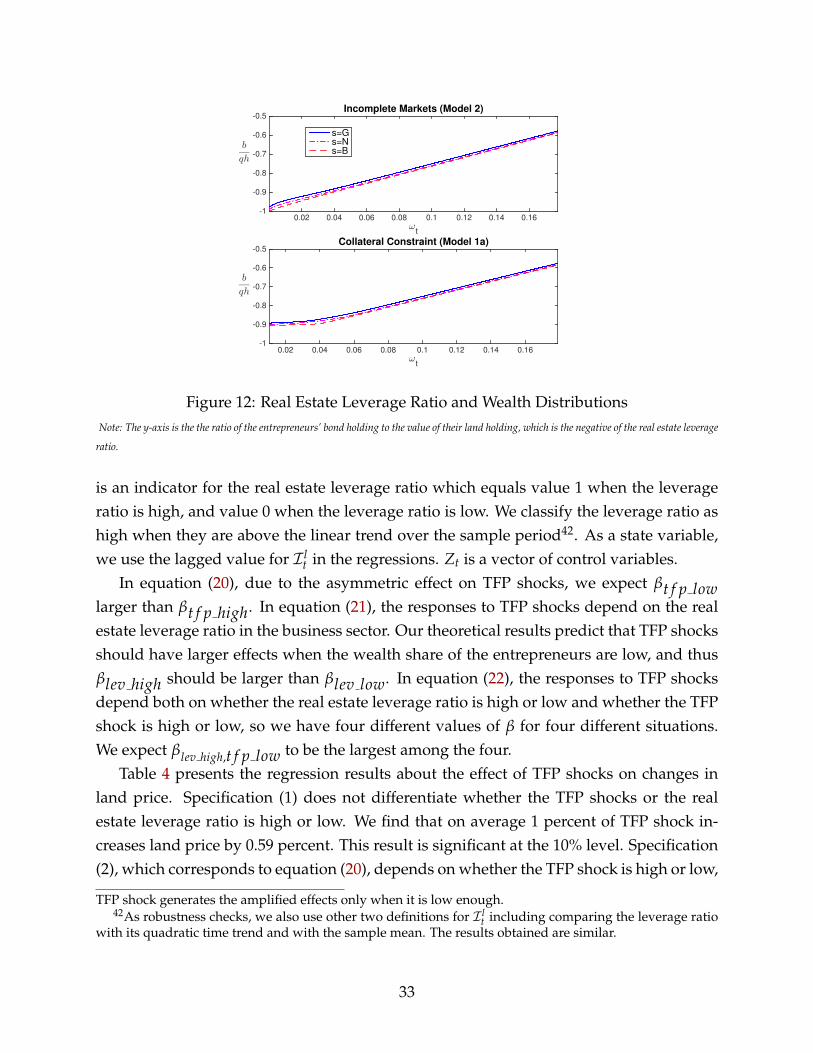
U.S. time series: the TFP shock, the real price of land, the real output and the real estateleverage ratio of the non-financial business (corporate and non-corporate) sector. The realestate leverage ratio is defined and constructed as the ratio of the credit market debt tothe value of real estate which is used as a proxy for the wealth share of the entrepreneurs.As can be seen from Figure 12, the real estate leverage ratio of the entrepreneurs is strictlydecreasing in their wealth share in incomplete markets model with or without collateralconstraints. The sample covers the period from 1951:Q4 to 2010:Q4. Appendix E providesmore detailed descriptions of the data.

Our specifications take the following three forms:

∆ log xt = α1 + βt f p highIt∆ log TFPt + βt f p low(1− It)∆ log TFPt + γ1Zt + ε1t (20)

∆ log xt = α2 + βlev highIlt−1∆ log TFPt + βlev low(1− I l

t−1)∆ log TFPt + γ2Zt + ε2t (21)

∆ log xt = α3 + βlev high, t f p highIlt−1It∆ log TFPt + βlev high,t f p lowI

lt−1(1− It)∆ log TFPt (22)

+ βlev low, t f p high(1− Ilt−1)It∆ log TFPt

+ βlev low,t f p low(1− I lt−1)(1− It)∆ log TFPt + γ3Zt−1 + ε2t

where xt is either real output or real land price, It is an indicator for TFP shock whichequals value 1 when TFP shocks are high, and value 0 when they are low41. Similarly, I l

t

41We use the first quintile of the TFP shocks as the threshold value. As indicated by our model, a negative

32

ωt

0.02 0.04 0.06 0.08 0.1 0.12 0.14 0.16

b

qh

-1

-0.9

-0.8

-0.7

-0.6

-0.5Incomplete Markets (Model 2)

s=G

s=N

s=B

ωt

0.02 0.04 0.06 0.08 0.1 0.12 0.14 0.16

b

qh

-1

-0.9

-0.8

-0.7

-0.6

-0.5Collateral Constraint (Model 1a)

Figure 12: Real Estate Leverage Ratio and Wealth DistributionsNote: The y-axis is the the ratio of the entrepreneurs’ bond holding to the value of their land holding, which is the negative of the real estate leverage

ratio.

is an indicator for the real estate leverage ratio which equals value 1 when the leverageratio is high, and value 0 when the leverage ratio is low. We classify the leverage ratio ashigh when they are above the linear trend over the sample period42. As a state variable,we use the lagged value for I l

t in the regressions. Zt is a vector of control variables.In equation (20), due to the asymmetric effect on TFP shocks, we expect βt f p low

larger than βt f p high. In equation (21), the responses to TFP shocks depend on the realestate leverage ratio in the business sector. Our theoretical results predict that TFP shocksshould have larger effects when the wealth share of the entrepreneurs are low, and thusβlev high should be larger than βlev low. In equation (22), the responses to TFP shocksdepend both on whether the real estate leverage ratio is high or low and whether the TFPshock is high or low, so we have four different values of β for four different situations.We expect βlev high,t f p low to be the largest among the four.

Table 4 presents the regression results about the effect of TFP shocks on changes inland price. Specification (1) does not differentiate whether the TFP shocks or the realestate leverage ratio is high or low. We find that on average 1 percent of TFP shock in-creases land price by 0.59 percent. This result is significant at the 10% level. Specification(2), which corresponds to equation (20), depends on whether the TFP shock is high or low,

TFP shock generates the amplified effects only when it is low enough.42As robustness checks, we also use other two definitions for I l

t including comparing the leverage ratiowith its quadratic time trend and with the sample mean. The results obtained are similar.

33

and shows that the asymmetric effect on this dimension is strong. The effect of a high TFPshock is small and not significant, while a low TFP shock has large and significant effectsuch that a 1% TFP shock has strong amplified effect of 1.83% on housing price. Specifica-tion (3), which corresponds to equation (21) shows that when the real estate leverage ratiois high, the responses are large and significant at 5% level. On the contrary, when the realestate leverage ratio is low, the responses to TFP shocks are insignificant. Specification (4),which corresponds to equation (22), combines the previous two cases of high or low TFPshock and high or low real estate leverage ratio, resulting in four possible combinations.We find that TFP shocks have significant effects on land price only when TFP shocks arelow, and the effect is the largest when we have both a high real estate leverage ratio anda low TFP shock. All the results shown here are consistent with the predictions of ourmodel.

Table 5 presents the regression results about the effect of TFP shocks on changes inreal GDP. Similarly, the coefficients show high asymmetric effects depending on whetherthe TFP shock or the real estate leverage ratio is high or low. Compared to the results ofland price in Table 4, the responses of output are smaller, but the asymmetric effects arevery robust.

The empirical findings in Tables 4 and 5 complement the recent results in Guerrieri andIacoviello (2015a), which emphasizes the asymmetric responses of economic activities,including consumption and employment, to changes in house prices. Using state andMSA-level data, they find that changes in economic activities correlate more with houseprices when house prices are low. This is consistent with our results because in our modelland price is strictly increasing in the entrepreneurs’ wealth share, and thus is strictlydecreasing in real estate leverage ratio.

6 Conclusion

In this paper, we have shown that market incompleteness, independently of the collat-eral constraint, plays a quantitatively significant role in the amplified and asymmetricresponses of the economy to exogenous shocks. For simplicity, we only consider one typeof shock - productivity shocks. However, it is easy to extend the paper to incorporateother shocks such as housing preference shocks. It would also be interesting to incor-porate money into the model to consider the effects of nominal versus inflation indexeddebts and of monetary shocks and as in Iacoviello (2005) and Cordoba and Ripoll (2004a).The current model does not have capital. We can consider adding capital into the modelto examine how the amplification and asymmetric effects affect the capital accumulation

34

and the aggregate production processes. Cao (2010) offers a way to introduce capital intothis kind of model which enables the use of a similar global nonlinear solution method tothe one in Subsection B. However, in this case we need to keep track of two endogenousstate variables: the wealth distribution and the aggregate capital.

References

Becker, R. (1980). On the long-run steady state in a simple dynamic model of equilibriumwith heterogeneous households. Quarterly Journal of Economics 95(2), 375–382.

Bianchi, J. (2011). Overborrowing and systemic externalities in the business cycle. Ameri-can Economic Review 101(7), 3400–3426.

Bianchi, J. and E. G. Mendoza (2013, December). Optimal time-consistent macropruden-tial policy. Working Paper 19704, National Bureau of Economic Research.

Brunnermeier, M. and Y. Sannikov (2014). A macroeconomic model with a financial sector.American Economic Reviews 104(2), 379–421.

Cao, D. (2010). Collateral shortages, asset price and investment volatility with heteroge-neous beliefs. Georgetown University Working Paper.

Cao, D. (2011). Speculation and financial wealth distribution under belief heterogeneity.Georgetown University Working Paper.

Cordoba, J. C. and M. Ripoll (2004a). Collateral constraints in a monetary economy. Jour-nal of the European Economic Association 2(6), 1172–1205.

Cordoba, J.-C. and M. Ripoll (2004b). Credit cycle redux. International Economic Re-view 45(4), 1011–1046.

Davis, M. A. and J. Heathcote (2007). The price and quantity of residential land in theunited states. Journal of Monetary Economics 54, 2595–2620.

DiTella, S. (2014). Uncertainty shocks and balance sheet recessions. Stanford GSB WorkingPaper.

Duffie, D., J. Geanakoplos, A. Mas-Colell, and A. McLennan (1994). Stationary markovequilibria. Econometrica 62(4), 745–781.

35

Fernald, J. G. (2014). A quarterly, utilization-adjusted series on total factor productivity.FRBSF Working Paper 2012-19.

Fostel, A. and J. Geanakoplos (2008). Leverage cycles and the anxious economy. AmericanEconomic Reviews 98(4), 1211–1244.

Gali, J. (1999). Technology, employment, and the business cycle: Do technology shocksexplain aggregate fluctuations? American Economic Review 89(1), 249–271.

Geanakoplos, J. (2010). Leverage cycles. In K. R. Daron Acemoglu and M. Woodford(Eds.), NBER Macroeconomics Annual 2009, Volume 24, pp. 1–65. University of ChicagoPress.

Guerrieri, L. and M. Iacoviello (2015a). Collateral constraints and macroeconomic asym-metries.

Guerrieri, L. and M. Iacoviello (2015b). Occbin: A toolkit for solving dynamic modelswith occasionally binding constraints easily. Journal of Monetary Economics 70, 22 – 38.

He, Z. and A. Krishnamurthy (2011). A model of capital and crises. The Review of EconomicStudies 82(2).

He, Z. and A. Krishnamurthy (2013). Intermediary asset pricing. American EconomicReviews 103(2), 732–770.

Iacoviello, M. (2005). House prices, borrowing constraints, and monetary policy in thebusiness cycle. American Economic Reviews 95(3), 739–64.

Jeanne, O. and A. Korinek (2013, January). Macroprudential regulation versus moppingup after the crash. Working Paper 18675, National Bureau of Economic Research.

Khan, A. and J. Thomas (2013). Credit shocks, and aggregate fluctuations in an economywith production heterogeneity. Journal of Political Economy 121(6), 1055–1106.

King, R. G., C. I. Plosser, and S. T. Rebelo (1988). Production, growth and business cycles.Journal of Monetary Economics 21(2), 195 – 232.

Kiyotaki, N. and J. Moore (1997). Credit cycles. Journal of Political Economy 105(2), 211–248.

Kocherlakota (2000). Creating business cycles through credit constraints. Minneapolis FedQuarterly Review 24(3), 2–10.

36

Krishnamurthy, A. (2003). Collateral constraints and the amplification mechanism. Jour-nal of Economic Theory 111, 277–292.

Krishnamurthy, A. (2010). Amplification mechanisms in liquidity crises. American Eco-nomic Journal: Macroeconomics 2(3), 1–30.

Kubler, F. and K. Schmedders (2003). Stationary equilibria in asset-pricing models withincomplete markets and collateral. Econometrica 71(6), 1767–1793.

Liu, Z., P. Wang, and T. Zha (2013). Land-price dynamics and macroeconomic fluctua-tions. Econometrica 81(3), 1147–1184.

Lorenzoni, G. (2008). Inefficient credit booms. The Review of Economic Studies 75(3), 809–833.

Mendoza, E. (2010). Sudden stops, financial crises and leverage. American Economic Re-views 100(5), 1941–1966.

Mian, A. and A. Sufi (2014). House of Debt. University of Chicao Press.

Rampini, A. A. and S. Viswanathan (2010). Collateral, risk management, and the distri-bution of debt capacity. The Journal of Finance 65(6), 2293–2322.

Shleifer, A. and R. Vishny (1997). The limits of arbitrage. Journal of Finance 52(1), 35–55.

Smets, F. and R. Wouters (2007). Shocks and frictions in us business cycles: A bayesiandsge approach. American Economic Review 97(3), 586–606.

Appendix

A Complete Markets

When markets are complete, because the entrepreneurs are less patient than the house-holds, they tend to consume all their net worth in the present. If they are risk-neutral asin Brunnermeier and Sannikov (2014), they will consume their entire net worth at time0, but in our model, they are risk-averse, so they consume their net worth overtime,and their wealth relative to the households’ wealth goes to zero as time goes to infin-ity. The entrepreneurs can do so by issuing equity to households thanks to frictionlessfinancial markets. We consider the long run limit, when the wealth of the entrepreneursapproaches zero. The economy converges to a representative household economy, with

37

the production technology of the entrepreneurs. Due to the Markovian feature of uncer-tainty, the endogenous variables depend only on the aggregate state st: xt = x (st).

Given that the households own the whole production sector, the marginal utility fromthe marginal profit per unit of land should be equal to the marginal utility of one unitof land consumption, i.e., (c′t)

−σ2 πt = j (h′t)−σh . To evaluate the marginal utility of con-

sumption, we observe that the households consume the whole output in the long runso

c′t = Yt = Athυt L1−υ

t .

From the equalization of the marginal utility from the marginal profit and the marginalutility from land consumption, and using the expression for wage and profit in Subsection2.3, we have

j (H − ht)−σh =

(Athυ

t L1−υt

)−σ2νAthν−1

t L1−νt . (23)

The consumption and labor trade-off equation (15) implies

(1− ν) Athνt L−ν

t

(Athυ

t L1−υt

)−σ2= Lη−1

t . (24)

The two equations (23) and (24) help us solve for the two unknowns (ht, Lt) for each At.Now, given πt as a function of At,ht, and Lt, land price is determined by the pricing

kernel using the marginal utility of the representative household:

q (st)− π (st) = ∑st+1|st

βu′ (ct+1 (st+1))

u′ (ct (st))q (st+1)Pr (st, st+1) .

Given the solution, we can compute the changes of land price and output after the shockst changes from normal to expansion or recession. The result is shown in the first row ofTable 1.

Under log utilities σ1 = σ2 = σh = 1 and linear cost of labor η = 1, i.e., the parametersin Table 2, (23) and (24) imply that ht ≡ h = ν

j+ν H and Lt ≡ L = 1− ν.

B Global Nonlinear Method

We solve the exact nonlinear equilibrium of the model using the algorithm in Kubler andSchmedders (2003) and Cao (2010). In particular, we solve for the Markov equilibriumin this economy. The original algorithm in Kubler and Schmedders (2003) is for endow-ment economies. Cao (2010) extends this algorithm to a production economy with capitalaccumulation. In the current paper, we show that the original algorithm works similarly

38

when we add labor choice as well as housing consumption decision of the households.We present the details of this algorithm for the benchmark model - Model 1a - but thisalgorithm can be adapted to Models 1b,2,3,4 with minor changes.

Our algorithm looks for a Markov equilibrium mapping from the financial wealthdistribution, ωt - defined in (8), and aggregate shock, st, to land price, qt and bond price,pt, the allocation {ct, ht, bt, c′t, h′t, b′t, L′t} and wage wt, as well as future financial wealthdistributions, ωt+1(st+1), depending on the realization of future aggregate shocks, st+1.Indeed given the mapping from ωt+1 to

{qt+1, ct+1, c′t+1

}, for each ωt and st, we can solve

for {pt, qt, wt} and {ct, ht, bt, µt, c′t, h′t, b′t, L′t} and ωt+1 using the equations (9),(10),(11),(12),(13), (14), (15), the budget constraints of the entrepreneurs and the households, the landand bond market clearing conditions, as well as the consistency of future wealth distribu-tions with current portfolio choices, equation (8) for each future state. Here, we follow theprocedure in Cao (2010), instead of the one in Kubler and Schmedders (2003), in solvingfor ωt+1 simultaneously with other unknowns. The additional equations needed to solvefor ωt+1 are equation (8) applied to each of the future state st+1: ωt+1 = qt+1(ωt+1,st+1)ht+bt

qt+1(ωt+1,st+1)H ,in which the mapping from future wealth distribution and exogenous state to land price,qt+1(ωt+1, st+1), is determined from the previous iteration of the algorithm. It is easy toverify that the number of unknowns are exactly the same as the number of equations.

We solve for the Markov equilibrium using backward induction. The algorithm startsby solving for the equilibrium mapping for 1-period economy. Then given the map-ping from t = 0 to t = 1 for T-period economy, we can solve for the mapping for(T + 1)-period economy following the procedure described above. The algorithm con-verges when the initial mappings for T−period economy and (T + 1)-period economyare sufficiently close to each other.

An important difference relative to Kubler and Schmedders (2003) and Cao (2010) isthat in Model 2 the entrepreneurs are only subject to the natural borrowing limit, thereforewhen ωt is exactly at the natural borrowing limit ωt = ωt = 0, ct = 0 and the first-order conditions (18) and (19) are not well-defined.43 To deal with this issue, we solveseparately the equilibrium of the economy at ωt. At ωt, we know ct = 0, so we solve for{ht, bt, c′t, h′t, b′t, L′t, ωt+1} given the same set of equations described above.44 Given thatthe behavior of the economy is highly nonlinear around ωt, when we discretize [ωt, 1],we put more points in the range of low values of ωt.45

43When the entrepreneurs have some labor endowment, ωt can actually be slightly negative.44We can show that ωt+1 = 0. In Appendix D, we provide an analytical example that it is possible (even

in finite horizon) to have ωt+1 = 0 and ct+1 = 0 but ht+1, qt+1 > 0.45Given that the households are allowed to borrow from the entrepreneurs, the upper bound for ωt

should exceed 1. However, ωt tends to fall below 1, because of the households’ tendency to lend given their

39

C Proof of Lemma 1

We prove this result by contradiction. Suppose that in a competitive equilibrium withthe optimal plan of the entrepreneurs {ct, ht, bt}t,st , there exists t∗ and history st∗

∗ suchthat ωt∗(st∗

∗ ) = qt∗(st∗∗ )ht∗−1(st∗−1

∗ ) + bt∗−1(st∗−1∗ ) < 0. Given the formula for the profit

maximization of the entrepreneurs and the definition of financial wealth ωt, the budgetconstraint (5) can be re-written as

ct∗(st∗∗ ) +

(qt∗(st∗

∗ )− πt∗(st∗∗ ))

ht∗(st∗∗ ) + pt∗(st∗

∗ )bt∗(st∗∗ ) ≤ qt∗(st∗

∗ )ωt∗(st∗∗ )H.

Pick a λ > 1, and consider an alternative trading and consumption plan{

ct, ht, bt}

t,st forthe entrepreneurs which is the same as the initial plan for t < t∗ but for t ≥ t∗:

{ct, ht, bt

}t>t∗,st|st∗∗

= {λct, λht, λbt}t>t∗,st|st∗∗

and

ct∗(st∗∗ ) = λct∗(st∗

∗ )− (λ− 1)qt∗(st∗∗ )ωt∗(st∗

∗ ) > ct∗(st∗∗ )

ht∗(st∗∗ ) = λht∗(st∗

∗ )

bt∗(st∗∗ ) = λbt∗(st∗

∗ ).

It is easy to verify that{

ct, ht, bt}

t,st satisfy all the constraints, including the no-Ponzischemes condition. Since ct ≥ 0 for all t′, st′ , ct ≥ ct for all t, st and ct∗(st∗

∗ ) > ct∗(st∗). Thiscontradicts the property that {ct, ht, bt}t,st is the optimal plan of the entrepreneurs. So bycontradiction ωt ≥ 0 for all t, st.

When 0 < σ1 ≤ 1, we prove by contradiction that any feasible plans of the en-trepreneurs must have positive financial wealth for all t, st. Suppose that in a competi-tive equilibrium, there is a feasible plan

{ct, ht, bt

}t,st of the entrepreneurs with ωt∗(st∗

∗ ) =

qt∗(st∗∗ )ht∗−1(st∗−1

∗ ) + bt∗−1(st∗−1∗ ) < 0 for some t∗ and history st∗

∗ . As argued above, thebudget constraint (5) can be re-written as

ct∗(st∗∗ ) +

(qt∗(st∗

∗ )− πt∗(st∗∗ ))

ht∗(st∗∗ ) + pt∗(st∗

∗ )bt∗(st∗∗ ) ≤ qt∗(st∗

∗ )ωt∗(st∗∗ )H.

Pick a λ > 1, and consider an alternative trading and consumption plan{

˜ct, ˜ht, ˜bt

}t,st

for

higher discount factor.

40

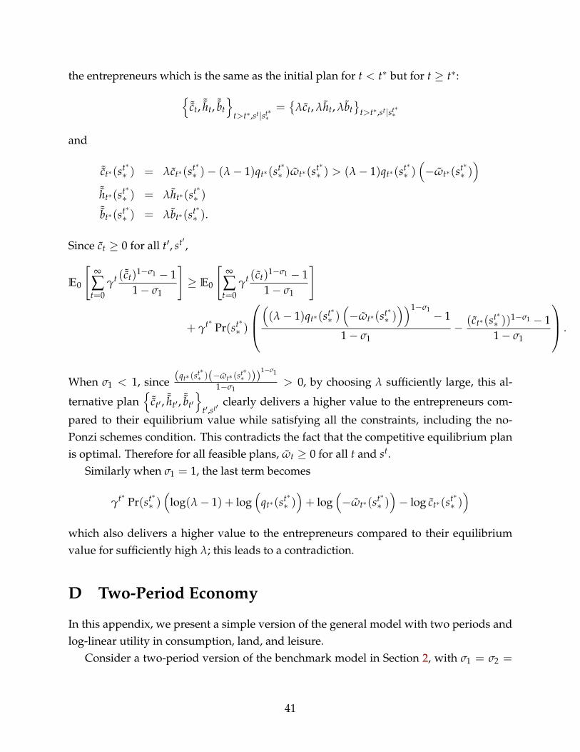
the entrepreneurs which is the same as the initial plan for t < t∗ but for t ≥ t∗:{˜ct, ˜ht, ˜bt

}t>t∗,st|st∗∗

={

λct, λht, λbt}

t>t∗,st|st∗∗

and

˜ct∗(st∗∗ ) = λct∗(st∗

∗ )− (λ− 1)qt∗(st∗∗ )ωt∗(st∗

∗ ) > (λ− 1)qt∗(st∗∗ )(−ωt∗(st∗

∗ ))

˜ht∗(st∗∗ ) = λht∗(st∗

∗ )˜bt∗(st∗

∗ ) = λbt∗(st∗∗ ).

Since ct ≥ 0 for all t′, st′ ,

E0

[∞

∑t=0

γt ( ˜ct)1−σ1 − 11− σ1

]≥ E0

[∞

∑t=0

γt (ct)1−σ1 − 11− σ1

]

+ γt∗ Pr(st∗∗ )

((λ− 1)qt∗(st∗

∗ )(−ωt∗(st∗

∗ )))1−σ1 − 1

1− σ1− (ct∗(st∗

∗ ))1−σ1 − 1

1− σ1

.

When σ1 < 1, since (qt∗ (st∗∗ )(−ωt∗ (st∗

∗ )))1−σ1

1−σ1> 0, by choosing λ sufficiently large, this al-

ternative plan{

˜ct′ ,˜ht′ ,

˜bt′}

t′,st′clearly delivers a higher value to the entrepreneurs com-

pared to their equilibrium value while satisfying all the constraints, including the no-Ponzi schemes condition. This contradicts the fact that the competitive equilibrium planis optimal. Therefore for all feasible plans, ωt ≥ 0 for all t and st.

Similarly when σ1 = 1, the last term becomes

γt∗ Pr(st∗∗ )(

log(λ− 1) + log(

qt∗(st∗∗ ))+ log

(−ωt∗(st∗

∗ ))− log ct∗(st∗

∗ ))

which also delivers a higher value to the entrepreneurs compared to their equilibriumvalue for sufficiently high λ; this leads to a contradiction.

D Two-Period Economy

In this appendix, we present a simple version of the general model with two periods andlog-linear utility in consumption, land, and leisure.

Consider a two-period version of the benchmark model in Section 2, with σ1 = σ2 =

41

σh = η = 1. That corresponds to the utility of the households,

E0

1

∑t=0

βt {log c′t + j log h′t − L′t}

.

and the utility of the entrepreneurs

E0

1

∑t=0

γt log ct.

At time t = 0, the entrepreneurs are endowed with a fraction ω0 of the total land sup-ply, and the households are endowed with the remaining fraction, 1−ω0. The sequentialbudget constraints, production function, and competitive and Markov equilibria underdifferent financial markets structure are defined as in the main body of the paper.

In order to solve for the Markov equilibrium of this economy, we first solve for theequilibrium in the last period t = T = 1 given the financial wealth share of the en-trepreneurs, ωT.46

The entrepreneurs maximize consumption,

maxcT ,hT ,LT

log cT

subject to the budget constraint

cT + qThT = qT HωT + AThυT L1−υ

T − wT LT.

From the F.O.Cs

wT = (1− υ)AT

(hT

LT

)υ

qT = υAt

(hT

LT

)υ−1

.

Substituting these expressions into the entrepreneurs’ budget constraint implies

cT = qT HωT.

46This financial wealth share is determined endogenously from the equilibrium in period t = T− 1, butat period T, the agents take it as given.

42

The households maximize

maxc′T ,h′T ,L′T

{log c′T + j log h′T − L′T}

subject toc′T + qTh′T = qT H(1−ωT) + wT L′T.

From the F.O.Cs in c′T, L′T, h′T:

c′T =wT

qT

c′T=

jh′T

.

ThereforeH − hT

j=

wT

qT=

(1− υ)

υ

hT

LT,

where the second equality comes from the F.O.Cs of the entrepreneurs. So

LT =j(1− υ)

υ

hT

H − hT

and

qT = υAT

[υ

j(1− υ)(H − hT)

]υ−1

.

Combining these results with the market clearing condition in the good markets: cT +

c′T = YT, we obtain

hT =1 + jωT

j/υ + 1H

h′T =j/υ− jωT

j/υ + 1H,

and

qT = υAT

[υ(1−ωTυ)

(1− υ)(j + υ)H]υ−1

. (25)

43

We can also solve for cT and c′T explicitly:

cT =qT HωT = υAT

[υ(1− υωT)

(1− υ)(j + υ)H]υ−1

HωT

c′T =υAT

[υ (1− υωT) H(1− υ)(j + υ)

]υ−1 (1− υωT) Hj + υ

.

These expressions also imply that

cT

c′T= (j + υ)

ωT

1− υωT, (26)

which is strictly increasing in ωT. We will use this result later when we analyze the twoperiod economy.

The following propositions summarize the key properties of the equilibrium in thelast period:

Proposition 1. qTAT

is strictly increasing in ωT and qT > 0 when ωT = 0.

Proof. From (25),qT

AT= υ

[υ(1−ωTυ)

(1− υ)(j + υ)H]υ−1

,

which is strictly increasing in ωT given that υ < 1. Moreover, when ωT = 0, qT =

υAT

[υ

(1−υ)(j+υ)H]υ−1

> 0.

Proposition 2. YTAT

and YTAT

are strictly increasing in ωT, where YT is the output taking intoaccount the imputed value of housing services to the household defined as in equation (7):

YT = YT + jc′T.

Moreover, YT and YT > 0 when ωT = 0.

Proof. After lengthy algebra manipulations, we arrive at

YT

AT= Hυυυ(1− υ)1−υ 1

(j + υ)υ1 + jωT

(1− υωT)1−υ

,

andYT

AT= Hυυυ(1− υ)1−υ 1

(j + υ)υ1 + j + j(1− υ)ωT

(1− υωT)1−υ

.

It is easy to see that both functions are strictly increasing in ωT and strictly positive evenwhen ωT = 0.

44

Propositions 1 and 2 show that, because the entrepreneurs are the only producers inthe economy, the more wealth (or land share) they own, the more they can use leverage topurchase more land for production. That leads to higher land price as well as aggregateoutput.

Given the equilibrium at t = T = 1, we consider the equilibrium of the economy att = T − 1 = 0 under two different financial markets structure. In the first case, financialmarkets are complete, i.e., from the first period t = T − 1 = 0, the entrepreneurs andhouseholds have access to a complete set of securities contingent on the realizations ofthe aggregate productivity AT in the second period. In the second case, financial marketsare incomplete, i.e. from the first period t = T− 1 = 0, the entrepreneurs and householdscan only trade bonds with payoff independent of the realizations of the aggregate pro-ductivity AT in the second period. Under complete markets, we show that qT

ATand YT

AT, YT

AT

are independent of AT. While under incomplete markets, we show that qTAT

and YTAT

, YTAT

arestrictly increasing in AT.

Complete Markets:At time t = 0, the entrepreneurs and households can trade state contingent securities -

φ0(s1) and φ′0(s1) denoting the holdings of the entrepreneurs and the households respec-tively - which pays off one unit of consumption good if state s1 is realized at t = 1 and0 otherwise. The prices of these securities are p0(s1) and are determined such that themarkets for these securities clear, i.e. φ0(s1) + φ′0(s1) = 0, for each s1. The entrepreneursand households can also trade in the land market at price q0, and land market clears, i.e.h0 + h′0 = H. The entrepreneurs are initially endowed with a fraction ω0 of the total stockof land.

At time t = 0, the entrepreneurs solve

maxc0,c1(.),h0,φ0(.),L0,h1(.),L1(.)

log c0 + γE [log c1]

subject to:c0 + q0h0 + ∑

s1

p0 (s1) φ0 (s1) = q0Hω0 + A0hυ0 L1−υ

0 − w0L0,

andc1 + q1h1 = q1Hω1 + A1hυ

1 L1−υ1 − w1L1,

where ω1 = q1h1+φ0(s1)q1H . The households maximize their inter-temporal expected utility

subject to similar constraints.Proposition 3 below shows that, with complete markets, land price and output at time

t = 1 are proportional to the realization of productivity A1.

45

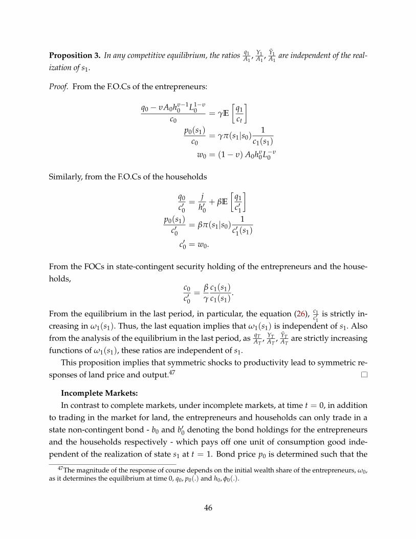
Proposition 3. In any competitive equilibrium, the ratios q1A1

, Y1A1

, Y1A1

are independent of the real-ization of s1.

Proof. From the F.O.Cs of the entrepreneurs:

q0 − υA0hυ−10 L1−υ

0c0

= γE

[q1

ct

]p0(s1)

c0= γπ(s1|s0)

1c1(s1)

w0 = (1− υ) A0hυ0 L−υ

0

Similarly, from the F.O.Cs of the households

q0

c′0=

jh′0

+ βE

[q1

c′1

]p0(s1)

c′0= βπ(s1|s0)

1c′1(s1)

c′0 = w0.

From the FOCs in state-contingent security holding of the entrepreneurs and the house-holds,

c0

c′0=

β

γ

c1(s1)

c1(s1).

From the equilibrium in the last period, in particular, the equation (26), c1c′1

is strictly in-creasing in ω1(s1). Thus, the last equation implies that ω1(s1) is independent of s1. Alsofrom the analysis of the equilibrium in the last period, as qT

AT, YT

AT, YT

ATare strictly increasing

functions of ω1(s1), these ratios are independent of s1.This proposition implies that symmetric shocks to productivity lead to symmetric re-

sponses of land price and output.47

Incomplete Markets:In contrast to complete markets, under incomplete markets, at time t = 0, in addition

to trading in the market for land, the entrepreneurs and households can only trade in astate non-contingent bond - b0 and b′0 denoting the bond holdings for the entrepreneursand the households respectively - which pays off one unit of consumption good inde-pendent of the realization of state s1 at t = 1. Bond price p0 is determined such that the

47The magnitude of the response of course depends on the initial wealth share of the entrepreneurs, ω0,as it determines the equilibrium at time 0, q0, p0(.) and h0, φ0(.).

46

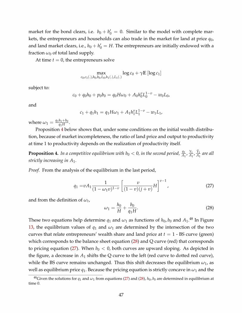
market for the bond clears, i.e. b0 + b′0 = 0. Similar to the model with complete mar-kets, the entrepreneurs and households can also trade in the market for land at price q0,and land market clears, i.e., h0 + h′0 = H. The entrepreneurs are initially endowed with afraction ω0 of total land supply.

At time t = 0, the entrepreneurs solve

maxc0,c1(.),h0,b0,L0,h1(.),L1(.)

log c0 + γE [log c1]

subject to:c0 + q0h0 + p0b0 = q0Hω0 + A0hυ

0 L1−υ0 − w0L0,

andc1 + q1h1 = q1Hω1 + A1hυ

1 L1−υ1 − w1L1,

where ω1 = q1h1+b0q1H .

Proposition 4 below shows that, under some conditions on the initial wealth distribu-tion, because of market incompleteness, the ratio of land price and output to productivityat time 1 to productivity depends on the realization of productivity itself.

Proposition 4. In a competitive equilibrium with b0 < 0, in the second period, q1A1

, Y1A1

, Y1A1

are allstrictly increasing in A1.

Proof. From the analysis of the equilibrium in the last period,

q1 =υA11

(1−ω1υ)1−υ

[υ

(1− υ)(j + υ)H]υ−1

, (27)

and from the definition of ωt,

ω1 =h0

H+

b0

q1H. (28)

These two equations help determine q1 and ω1 as functions of h0, b0 and A1.48 In Figure13, the equilibrium values of q1 and ω1 are determined by the intersection of the twocurves that relate entrepreneurs’ wealth share and land price at t = 1 - BS curve (green)which corresponds to the balance sheet equation (28) and Q curve (red) that correspondsto pricing equation (27). When b0 < 0, both curves are upward sloping. As depicted inthe figure, a decrease in A1 shifts the Q curve to the left (red curve to dotted red curve),while the BS curve remains unchanged. Thus this shift decreases the equilibrium ω1, aswell as equilibrium price q1. Because the pricing equation is strictly concave in ω1 and the

48Given the solutions for q1 and ω1 from equations (27) and (28), h0, b0 are determined in equilibrium attime 0.

47

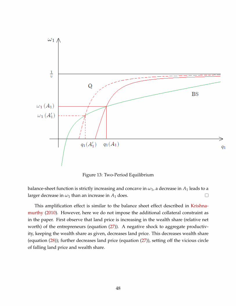
Figure 13: Two-Period Equilibrium

balance-sheet function is strictly increasing and concave in ω1, a decrease in A1 leads to alarger decrease in ω1 than an increase in A1 does.

This amplification effect is similar to the balance sheet effect described in Krishna-murthy (2010). However, here we do not impose the additional collateral constraint asin the paper. First observe that land price is increasing in the wealth share (relative networth) of the entrepreneurs (equation (27)). A negative shock to aggregate productiv-ity, keeping the wealth share as given, decreases land price. This decreases wealth share(equation (28)); further decreases land price (equation (27)), setting off the vicious circleof falling land price and wealth share.

48

E Data Description and Empirical Results

Our empirical results are based on four U.S. aggregate series: the TFP shock, the real priceof land, the real output and the real estate leverage ratio in the non-financial business sec-tor. The data of real price of land covers the period 1975:Q1 to 2010:Q4. For the other threeseries, the sample period is from 1951:Q4 to 2014:Q4. All series are seasonally adjustedusing the X-13ARIMA-SEATS program provided by the U.S. Census Bureau.

The TFP shock is retrieved from Federal Reserve Bank of St. Louis. We use utilization-adjusted quarterly-TFP series for the U.S. Business Sector, produced by John Fernald (Fer-nald, 2014). We divide the original series by four to cancel his annualization adjustment.

The real price of land is from Liu, Wang, and Zha (2013). As claimed in their paper,fluctuations in real estate values are mostly driven by changes in land prices. They useliquidity-adjusted price index for residential land, which they construct from the FHFAHome Price Index using the method provided in Davis and Heathcote (2007) . The seriesis adjusted using the price index of nondurables consumption and services from Bureauof Economic Analysis. See Appendix A of their paper for more details on this series.

The real output data is the real GDP from Federal Reserve Bank of St. Louis usingchained dollars method (2009=100). We divide the original series by four to cancel theirannualization adjustment.

The real estate leverage ratio is the ratio of the net value of credit market debt (creditmarket debt - credit market instruments) to the market value of real estate in the non-financial business sector. All the data used to construct this ratio is from the FinancialAccounts of United States provided by the Federal Reserve Board.

49

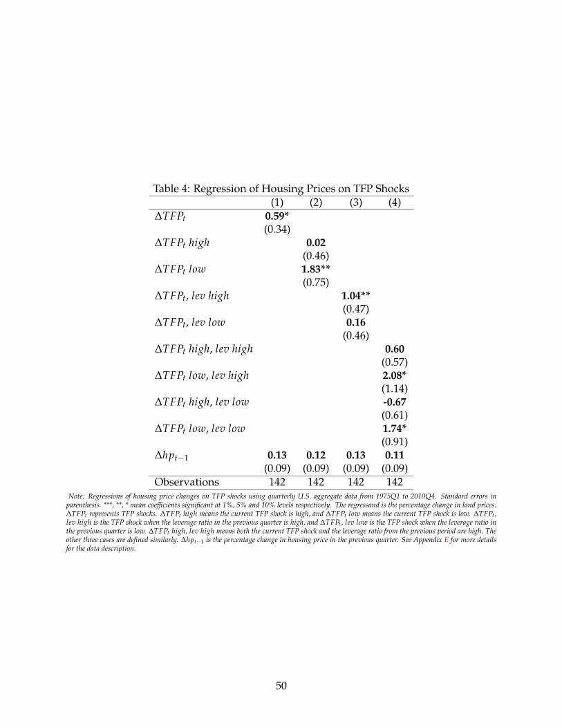
Table 4: Regression of Housing Prices on TFP Shocks(1) (2) (3) (4)

∆TFPt 0.59*(0.34)

∆TFPt high 0.02(0.46)

∆TFPt low 1.83**(0.75)

∆TFPt, lev high 1.04**(0.47)

∆TFPt, lev low 0.16(0.46)

∆TFPt high, lev high 0.60(0.57)

∆TFPt low, lev high 2.08*(1.14)

∆TFPt high, lev low -0.67(0.61)

∆TFPt low, lev low 1.74*(0.91)

∆hpt−1 0.13 0.12 0.13 0.11(0.09) (0.09) (0.09) (0.09)

Observations 142 142 142 142Note: Regressions of housing price changes on TFP shocks using quarterly U.S. aggregate data from 1975Q1 to 2010Q4. Standard errors in

parenthesis. ***, **, * mean coefficients significant at 1%, 5% and 10% levels respectively. The regressand is the percentage change in land prices.∆TFPt represents TFP shocks. ∆TFPt high means the current TFP shock is high, and ∆TFPt low means the current TFP shock is low. ∆TFPt,lev high is the TFP shock when the leverage ratio in the previous quarter is high, and ∆TFPt, lev low is the TFP shock when the leverage ratio inthe previous quarter is low. ∆TFPt high, lev high means both the current TFP shock and the leverage ratio from the previous period are high. Theother three cases are defined similarly. ∆hpt−1 is the percentage change in housing price in the previous quarter. See Appendix E for more detailsfor the data description.

50

Table 5: Regression of Real Output on TFP Shocks(1) (2) (3) (4)

∆TFPt 0.11***(0.03)

∆TFPt high 0.065*(0.04)

∆TFPt low 0.21***(0.07)

∆TFPt, lev high 0.16***(0.04)

∆TFPt, lev low 0.05(0.04)

∆TFPt high, lev high 0.13***(0.046)

∆TFPt low, lev high 0.20**(0.09)

∆TFPt high, lev low -0.02(0.05)

∆TFPt low, lev low 0.23**(0.09)

∆outputt−1 0.38*** 0.37*** 0.37*** 0.36***(0.06) (0.06) (0.06) (0.06)

Observations 252 252 252 252Note: Regressions of real GDP changes on TFP shocks using quarterly U.S. aggregate data from 1951Q4 to 2014Q4. Standard errors in parenthe-

sis. ***, **, * mean coefficients significant at 1%, 5% and 10% levels respectively. The regressand is the percentage change in land prices. ∆TFPtrepresents TFP shocks. ∆TFPt high means the current TFP shock is high, and ∆TFPt low means the current TFP shock is low. ∆TFPt, lev high isthe TFP shock when the leverage ratio in the previous quarter is high, and ∆TFPt, lev low is the TFP shock when the leverage ratio in the previousquarter is low. ∆TFPt high, lev high means both the current TFP shock and the leverage ratio from the previous period are high. The other threecases are defined similarly. ∆outputt−1 is the percentage change in real GDP in the previous quarter. See Appendix E for more details for the datadescription.

51

F Steady State and Log-Linearization for Collateral Con-

straint Model

Becker (1980) shows that in a neoclassical growth model with heterogeneous discountfactors, long run wealth concentrates on the most patient agents, in this case the house-holds. However, in our model, due to the collateral constraint, the entrepreneurs can onlypledge a fraction of their future wealth to borrow. Therefore, despite their lower discountfactor, their wealth does not disappear in the long run. In particular, the model admitsa long run steady state in the absence of uncertainty. In this subsection, we solve for thesteady state in our model.

Suppose that there is no uncertainty, i.e., At(st) ≡ A. In steady state, all variables areconstant, so we can omit the subscript t. For the ease of notation, denote

γe = mβ + (1−m)γ, (29)

as the average discount factor for the entrepreneurs’ investment in land as in Iacoviello(2005). The first order condition in b′t ,

b′t : −ptc

′−σ2t + βEt

[c′−σ2

t+1

]= 0, (30)

in the steady state, c′t = c′t+1 = c′, implies that p = β. Because γ < β, the entrepreneurwants to borrow as much as possible up to the collateral constraint. Indeed, the first ordercondition for b implies that the collateral constraint is strictly binding and the Lagrangemultiplier µ on the constraint is strictly positive:

µ = (β− γ) c−σ1 > 0. (31)

Given that the collateral constraint is binding, we have b = −mqh.From the first-order condition in h,

(πt − qt)c−σ1t + µtmEt [qt+1] + γEt

[qt+1c−σ1

t+1

]= 0, (32)

in which the marginal profit

πt = νAt

(ht

Lt

)ν−1

In the steady state, we have

q =1

1− γeυAhυ−1L1−υ. (33)

52

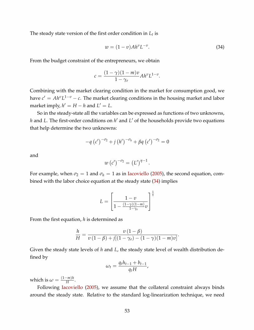
The steady state version of the first order condition in Lt is

w = (1− υ)AhυL−υ. (34)

From the budget constraint of the entrepreneurs, we obtain

c =(1− γ)(1−m)υ

1− γeAhυL1−υ.

Combining with the market clearing condition in the market for consumption good, wehave c′ = AhυL1−υ − c. The market clearing conditions in the housing market and labormarket imply, h′ = H − h and L′ = L.

So in the steady-state all the variables can be expressed as functions of two unknowns,h and L. The first-order conditions on h′ and L′ of the households provide two equationsthat help determine the two unknowns:

−q(c′)−σ2 + j

(h′)−σh + βq

(c′)−σ2 = 0

andw(c′)−σ2 =

(L′)η−1 .

For example, when σ2 = 1 and σh = 1 as in Iacoviello (2005), the second equation, com-bined with the labor choice equation at the steady state (34) implies

L =

1− υ

1− (1−γ)(1−m)1−γe

υ

1η

From the first equation, h is determined as

hH

=υ (1− β)

υ (1− β) + j[(1− γe)− (1− γ)(1−m)υ].

Given the steady state levels of h and L, the steady state level of wealth distribution de-fined by

ωt =qtht−1 + bt−1

qtH,

which is ω = (1−m)hH .

Following Iacoviello (2005), we assume that the collateral constraint always bindsaround the steady state. Relative to the standard log-linearization technique, we need

53

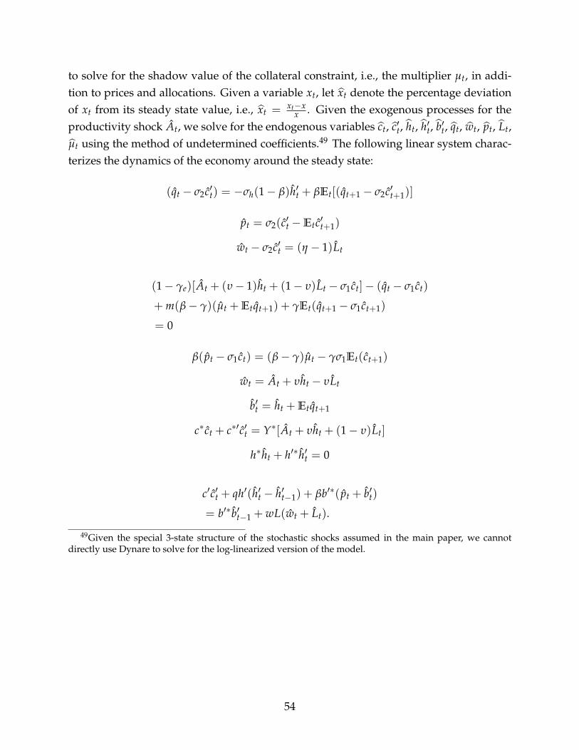
to solve for the shadow value of the collateral constraint, i.e., the multiplier µt, in addi-tion to prices and allocations. Given a variable xt, let xt denote the percentage deviationof xt from its steady state value, i.e., xt = xt−x

x . Given the exogenous processes for theproductivity shock At, we solve for the endogenous variables ct, c′t, ht, h′t, b′t, qt, wt, pt, Lt,µt using the method of undetermined coefficients.49 The following linear system charac-terizes the dynamics of the economy around the steady state:

(qt − σ2c′t) = −σh(1− β)h′t + βEt[(qt+1 − σ2c′t+1)]

pt = σ2(c′t −Et c′t+1)

wt − σ2c′t = (η − 1)Lt

(1− γe)[At + (υ− 1)ht + (1− υ)Lt − σ1ct]− (qt − σ1ct)

+ m(β− γ)(µt + Etqt+1) + γEt(qt+1 − σ1ct+1)

= 0

β( pt − σ1ct) = (β− γ)µt − γσ1Et(ct+1)

wt = At + υht − υLt

b′t = ht + Etqt+1

c∗ ct + c∗′ c′t = Y∗[At + υht + (1− υ)Lt]

h∗ht + h′∗h′t = 0

c′ c′t + qh′(h′t − h′t−1) + βb′∗( pt + b′t)

= b′∗b′t−1 + wL(wt + Lt).

49Given the special 3-state structure of the stochastic shocks assumed in the main paper, we cannotdirectly use Dynare to solve for the log-linearized version of the model.

54

G Stationary State under Collateral Constraint with Com-

plete Markets

We show that with the parameters chosen in our calibration, in particular, σ1 = σ2 = σh =

1 and η = 1, the stationary distribution of wealth share is degenerated: ωt ≡ ω∗50. Thenall the endogenous variables x(ωt, st) can be written as x(st), and the holdings of Arrowsecurities φ (ωt, st, st+1) as φ (st, st+1) and their prices as p (st, st+1). We conjecture andverify below that the collateral constraints are always binding. Thus the entrepreneurs’holdings of Arrow securities are

φ (st, st+1) = −mq (st+1) h (st) , (35)

which implies ωt+1 = (1−m) htH . In order for ωt ≡ ω∗, we must have ht ≡ h∗. We make

an additional conjecture about the households’ labor supply: Lt = L∗. We will verifythese conjectures step by step.

Since η = 1, from the households’ labor-leisure choice, we have

c′ (st) = wage = (1− ν)A (st)

(h∗

L∗

)ν (36)

and

c (st) = Y (st)− c′ (st)

= A (st) (h∗)ν (L∗)−ν [L∗ − (1− ν)] (37)

The first-order condition with respect to φ′t (st, st+1) implies

p (st, st+1) =βπ(st+1|st)c′ (st)

c′ (st+1)=

βπ(st+1|st)A (st)

A (st+1). (38)

Denote the Lagrangian multipliers as µ (st, st+1), the first-order-condition of φt (st, st+1)

is− p (st, st+1)

c (st)+ µ (st, st+1) +

γπ(st+1|st)

c (st+1)= 0

50With other commonly used parameter values, we find that the ergodic distribution has very smallvariance if not degenerated. For example, in an exercise with σ1 = σ2 = σh = 2 and η = 1.5, the meanwealth distribution ω is 0.0206, and the standard deviation is 8.7× 10−5.

55

Thus we have

µ (st, st+1) = π(st+1|st)

[βA(st)

c (st) A(st+1)− γ

c (st+1)

]=

π(st+1|st)(β− γ)

A (st+1) (h∗)ν (L∗)−ν [L∗ − (1− ν)]

Plugging this expression for µ (st, st+1) into the F.O.C. in ht

νA (st) (h∗)ν−1 (L∗)1−ν − q(st)

c(st)+m ∑

st+1|st

µ (st, st+1) q(st+1)+γ ∑st+1|st

π(st+1|st)q(st+1)

c(st+1)= 0

ν (h∗)ν−1 (L∗)1−ν − q(st)

A (st)+ γe ∑

st+1|st

π(st+1|st)q(st+1)

A(st+1)= 0

in which γe is given by (29).{

q(st)A(st)

}∀st ∈ S can be solved by the following system of

linear equations

[IS − γeΠ]

q(s1)A(s1)q(s2)A(s2)

...q(sS)A(sS)

= ν (h∗)ν−1 (L∗)1−ν

11...1

in which Π is the transition matrix for the Markov TFP shock process and IS is a S-dimensional identity matrix. After some matrix operation51, we get

q(s1)A(s1)q(s2)A(s2)

...q(sS)A(sS)

=1γe

ν (h∗)ν−1 (L∗)1−ν

11...1

Thus we have

q(s)A (s)

≡ 1γe

ν (h∗)ν−1 (L∗)1−ν , ∀s = 1, 2, . . . S. (39)

Lastly, h∗ must be determined so that the first-order conditions in the housing choiceof the household are satisfied in all states:

q (st)

c′ (st)− β ∑

st+1|st

π(st+1|st)q (st+1)

c′ (st+1)=

jH − h∗

,

51We use the fact that(

IS + γeΠ + γ2e Π2 + γ3

e Π3 + . . .)(IS − γeΠ) = IS

56

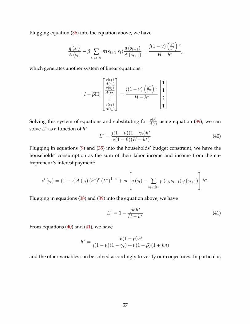
Plugging equation (36) into the equation above, we have

q (st)

A (st)− β ∑

st+1|st

π(st+1|st)q (st+1)

A (st+1)=

j(1− ν)(

h∗L∗

)ν

H − h∗,

which generates another system of linear equations:

[I − βΠ]

q(s1)A(s1)q(s2)A(s2)

...q(sS)A(sS)

=j(1− ν)

(h∗L∗

)ν

H − h∗

11...1

Solving this system of equations and substituting for q(s)

A(s) using equation (39), we cansolve L∗ as a function of h∗:

L∗ =j(1− ν)(1− γe)h∗

ν(1− β)(H − h∗)(40)

Plugging in equations (9) and (35) into the households’ budget constraint, we have thehouseholds’ consumption as the sum of their labor income and income from the en-trepreneur’s interest payment:

c′ (st) = (1− ν)A (st) (h∗)ν (L∗)1−ν + m

q (st)− ∑st+1|st

p (st, st+1) q (st+1)

h∗.

Plugging in equations (38) and (39) into the equation above, we have

L∗ = 1− jmh∗

H − h∗(41)

From Equations (40) and (41), we have

h∗ =ν(1− β)H

j(1− ν)(1− γe) + ν(1− β)(1 + jm)

and the other variables can be solved accordingly to verify our conjectures. In particular,

57

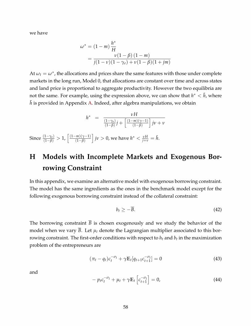
we have

ω∗ = (1−m)h∗

H

=ν(1− β) (1−m)

j(1− ν)(1− γe) + ν(1− β)(1 + jm)

At ωt = ω∗, the allocations and prices share the same features with those under completemarkets in the long run, Model 0, that allocations are constant over time and across statesand land price is proportional to aggregate productivity. However the two equilibria arenot the same. For example, using the expression above, we can show that h∗ < h, whereh is provided in Appendix A. Indeed, after algebra manipulations, we obtain

h∗ =νH

(1−γe)(1−β)

j +[(1−m)(γ−1)

(1−β)

]jν + ν

Since (1−γe)(1−β)

> 1,[(1−m)(γ−1)

(1−β)

]jν > 0, we have h∗ < νH

j+ν = h.

H Models with Incomplete Markets and Exogenous Bor-

rowing Constraint

In this appendix, we examine an alternative model with exogenous borrowing constraint.The model has the same ingredients as the ones in the benchmark model except for thefollowing exogenous borrowing constraint instead of the collateral constraint:

bt ≥ −B. (42)

The borrowing constraint B is chosen exogenously and we study the behavior of themodel when we vary B. Let µt denote the Lagrangian multiplier associated to this bor-rowing constraint. The first-order conditions with respect to ht and bt in the maximizationproblem of the entrepreneurs are

(πt − qt)c−σ1t + γEt[qt+1c−σ1

t+1 ] = 0 (43)

and− ptc

−σ1t + µt + γEt

[c−σ1

t+1

]= 0, (44)

58

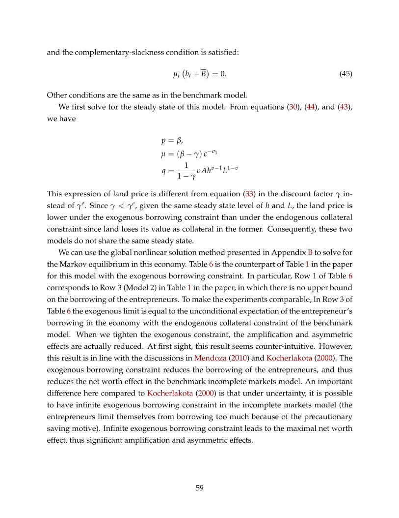
and the complementary-slackness condition is satisfied:

µt(bt + B

)= 0. (45)

Other conditions are the same as in the benchmark model.We first solve for the steady state of this model. From equations (30), (44), and (43),

we have

p = β,

µ = (β− γ) c−σ1

q =1

1− γυAhυ−1L1−υ

This expression of land price is different from equation (33) in the discount factor γ in-stead of γe. Since γ < γe, given the same steady state level of h and L, the land price islower under the exogenous borrowing constraint than under the endogenous collateralconstraint since land loses its value as collateral in the former. Consequently, these twomodels do not share the same steady state.

We can use the global nonlinear solution method presented in Appendix B to solve forthe Markov equilibrium in this economy. Table 6 is the counterpart of Table 1 in the paperfor this model with the exogenous borrowing constraint. In particular, Row 1 of Table 6corresponds to Row 3 (Model 2) in Table 1 in the paper, in which there is no upper boundon the borrowing of the entrepreneurs. To make the experiments comparable, In Row 3 ofTable 6 the exogenous limit is equal to the unconditional expectation of the entrepreneur’sborrowing in the economy with the endogenous collateral constraint of the benchmarkmodel. When we tighten the exogenous constraint, the amplification and asymmetriceffects are actually reduced. At first sight, this result seems counter-intuitive. However,this result is in line with the discussions in Mendoza (2010) and Kocherlakota (2000). Theexogenous borrowing constraint reduces the borrowing of the entrepreneurs, and thusreduces the net worth effect in the benchmark incomplete markets model. An importantdifference here compared to Kocherlakota (2000) is that under uncertainty, it is possibleto have infinite exogenous borrowing constraint in the incomplete markets model (theentrepreneurs limit themselves from borrowing too much because of the precautionarysaving motive). Infinite exogenous borrowing constraint leads to the maximal net wortheffect, thus significant amplification and asymmetric effects.

59

Table 6: Average land price and output changes in normal state, 3% shockLand price Output

Type of Friction Expansion Recession Expansion RecessionComplete Markets (Model 0) 3.00% 3.00% 3.00% 3.00%Collateral Constraint (Model 1a) 3.61% -4.22% 3.22% -3.62%incomplete markets (B = ∞, Model 2) 3.47% -3.81% 3.18% -3.40%incomplete markets (B = 2.73) 3.48% -3.53% 3.21% -3.26%

Table 7: Probabilities of Binding Collateral Constraint∆ Expansion Normal Recession Overall

0.1% 100% 100% 100% 100%0.5% 5.3% 90.7% 99.9% 78.7%1% 0.2% 42.9% 95.5% 44.4%2% 0% 4.9% 68.9% 14.2%3% 0% 0.2% 44.5% 7.1%4% 0% 0% 29.1% 4.6%5% 0% 0% 19.2% 3.0%

I Volatility Paradox

In Brunnermeier and Sannikov (2014), the authors discover an interesting feature calledvolatility paradox, i.e., with incomplete financial market, lower exogenous risk can lead tohigher endogenous risk. Their intuition is that lower exogenous risk encourages the en-trepreneurs to borrow more and use higher leverage which result in larger output/assetprice declines during crisis. We first show that in Model 1a with collateral constraint, ourfully nonlinear solution does not exhibit the volatility paradox because the entrepreneurs’borrowing capacity is constrained. As we decrease the size of the exogenous shocks, thebinding probability goes to 1 and the nonlinear solution becomes closer to the log-linearsolution, and both converge to the steady state with no endogenous risk. See Table 7 forthe details. The stationary distribution is thus degenerated, as shown in Figure 14 withdifferent sizes of exogenous shocks.

On the contrary, in Model 2 with incomplete market but no collateral constraint, werecover the volatility paradox. The stationary distribution is not degenerated when thesize of the exogenous shock goes to 0, as shown in Figure 15.

60

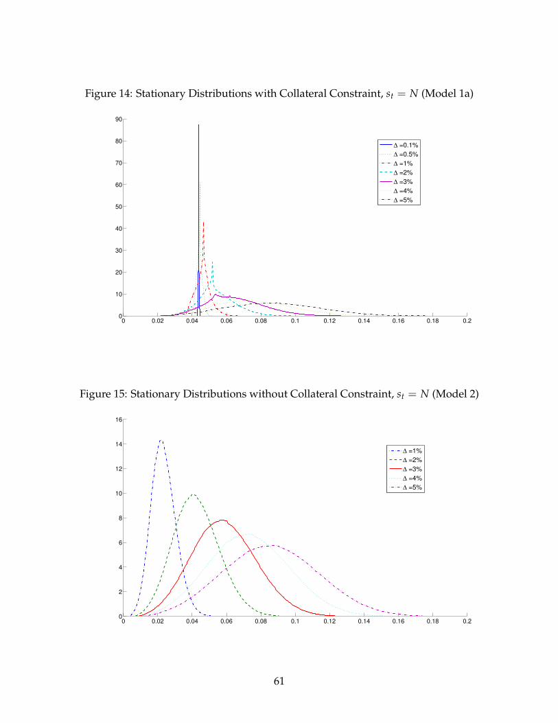
Figure 14: Stationary Distributions with Collateral Constraint, st = N (Model 1a)

0 0.02 0.04 0.06 0.08 0.1 0.12 0.14 0.16 0.18 0.20

10

20

30

40

50

60

70

80

90

∆ =0.1%

∆ =0.5%

∆ =1%

∆ =2%

∆ =3%

∆ =4%

∆ =5%

Figure 15: Stationary Distributions without Collateral Constraint, st = N (Model 2)

0 0.02 0.04 0.06 0.08 0.1 0.12 0.14 0.16 0.18 0.20

2

4

6

8

10

12

14

16

∆ =1%

∆ =2%

∆ =3%

∆ =4%

∆ =5%

61

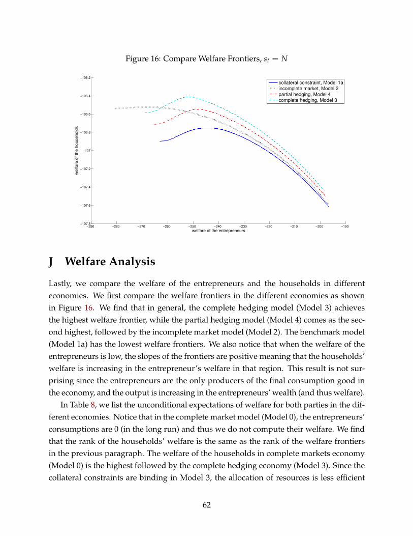
Figure 16: Compare Welfare Frontiers, st = N

−290 −280 −270 −260 −250 −240 −230 −220 −210 −200 −190−107.8

−107.6

−107.4

−107.2

−107

−106.8

−106.6

−106.4

−106.2

welfare of the entrepreneurs

welfare

of th

e h

ousehold

s

collateral constraint, Model 1aincomplete market, Model 2

partial hedging, Model 4complete hedging, Model 3

J Welfare Analysis

Lastly, we compare the welfare of the entrepreneurs and the households in differenteconomies. We first compare the welfare frontiers in the different economies as shownin Figure 16. We find that in general, the complete hedging model (Model 3) achievesthe highest welfare frontier, while the partial hedging model (Model 4) comes as the sec-ond highest, followed by the incomplete market model (Model 2). The benchmark model(Model 1a) has the lowest welfare frontiers. We also notice that when the welfare of theentrepreneurs is low, the slopes of the frontiers are positive meaning that the households’welfare is increasing in the entrepreneur’s welfare in that region. This result is not sur-prising since the entrepreneurs are the only producers of the final consumption good inthe economy, and the output is increasing in the entrepreneurs’ wealth (and thus welfare).

In Table 8, we list the unconditional expectations of welfare for both parties in the dif-ferent economies. Notice that in the complete market model (Model 0), the entrepreneurs’consumptions are 0 (in the long run) and thus we do not compute their welfare. We findthat the rank of the households’ welfare is the same as the rank of the welfare frontiersin the previous paragraph. The welfare of the households in complete markets economy(Model 0) is the highest followed by the complete hedging economy (Model 3). Since thecollateral constraints are binding in Model 3, the allocation of resources is less efficient

62

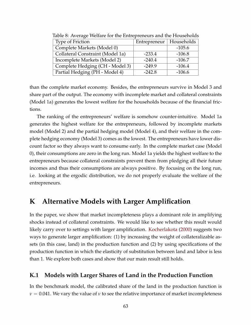
Table 8: Average Welfare for the Entrepreneurs and the HouseholdsType of Friction Entrepreneur HouseholdsComplete Markets (Model 0) -105.6Collateral Constraint (Model 1a) -233.4 -106.8Incomplete Markets (Model 2) -240.4 -106.7Complete Hedging (CH - Model 3) -249.9 -106.4Partial Hedging (PH - Model 4) -242.8 -106.6

than the complete market economy. Besides, the entrepreneurs survive in Model 3 andshare part of the output. The economy with incomplete market and collateral constraints(Model 1a) generates the lowest welfare for the households because of the financial fric-tions.

The ranking of the entrepreneurs’ welfare is somehow counter-intuitive. Model 1agenerates the highest welfare for the entrepreneurs, followed by incomplete marketsmodel (Model 2) and the partial hedging model (Model 4), and their welfare in the com-plete hedging economy (Model 3) comes as the lowest. The entrepreneurs have lower dis-count factor so they always want to consume early. In the complete market case (Model0), their consumptions are zero in the long run. Model 1a yields the highest welfare to theentrepreneurs because collateral constraints prevent them from pledging all their futureincomes and thus their consumptions are always positive. By focusing on the long run,i.e. looking at the ergodic distribution, we do not properly evaluate the welfare of theentrepreneurs.

K Alternative Models with Larger Amplification

In the paper, we show that market incompleteness plays a dominant role in amplifyingshocks instead of collateral constraints. We would like to see whether this result wouldlikely carry over to settings with larger amplification. Kocherlakota (2000) suggests twoways to generate larger amplification: (1) by increasing the weight of collateralizable as-sets (in this case, land) in the production function and (2) by using specifications of theproduction function in which the elasticity of substitution between land and labor is lessthan 1. We explore both cases and show that our main result still holds.

K.1 Models with Larger Shares of Land in the Production Function

In the benchmark model, the calibrated share of the land in the production function isν = 0.041. We vary the value of ν to see the relative importance of market incompleteness

63

Table 9: Average land price and output changes in normal state, 3% shockLand price Output

Type of Friction Expansion Recession Expansion RecessionIncomplete Markets (ν = 0.03) 3.34% -3.61% 3.11% -3.28%Collateral Constraint (ν = 0.03) 3.45% -3.95% 3.14% -3.47%Incomplete Markets (ν = 0.041) 3.47% -3.81% 3.18% -3.40%Collateral Constraint (ν = 0.041) 3.61% -4.22% 3.22% -3.62%Incomplete Markets (ν = 0.05) 3.56% -3.97% 3.24% -3.49%Collateral Constraint (ν = 0.05) 3.72% -4.40% 3.29% -3.71%Incomplete Markets (ν = 0.06) 3.66% -4.13% 3.30% -3.60%Collateral Constraint (ν = 0.06) 3.85% -4.59% 3.37% -3.82%Incomplete Markets (ν = 0.07) 3.76% -4.29% 3.37% -3.70%Collateral Constraint (ν = 0.07) 3.96% -4.76% 3.45% -3.93%

and collateral constraint in amplifying shocks. Other parameter values are not changed.The results are listed in Table 9 with two types of financial market structures: incompletemarkets structure without borrowing constraint, and incomplete markets with collateralconstraint.

First, we can see that as ν gets larger, the amplification effect is stronger. For example,with 3% negative TFP shock and collateral constraint, land price will decrease by -3.95%when ν = 0.03, but when ν = 0.07, land price decreases by -4.76%. Second, as ν getslarger, market incompleteness by itself explains a larger part in the total amplification ef-fect. With ν = 0.03 and a 3% negative TFP shock, output decreases by -3.28% with marketincompleteness alone compared to -3.47% in the economy with collateral constraint. Asa result, about 60% (3.28%−3%

3.47%−3% ) of the amplification effect is generated by market incom-pleteness. When ν = 0.07, this ratio increases to 75% (3.70%−3%

3.93%−3% ). The comparison suggeststhat in situations with larger amplification, market incompleteness quantitatively plays alarger role in amplifying shocks, and collateral constraint plays a smaller role. This resultshould not be surprising because with larger amplification, the entrepreneur’s precau-tionary saving motive is stronger and she will borrow less to avoid regions where thecollateral constraint is binding. Although in regions with binding collateral constraint,higher ν generates stronger amplification, the probability of the economy to enter thoseregions are lower. The binding probabilities with different ν are listed in Table 10. Onaverage collateral constraint has less effect in amplifying shocks as ν gets larger.

64

Table 10: Probabilities of Binding Collateral Constraintν Expansion Normal Recession Overall

0.03 0% 3.64% 51.11% 10.52%0.041 0% 0.18% 44.48% 7.11%0.05 0% 0% 40.07% 6.29%0.06 0% 0% 35.72% 5.61%0.07 0% 0% 32.13% 5.04%

Table 11: Average land price and output changes with CES production, 3% shockLand price Output

Type of Friction Expansion Recession Expansion RecessionCollateral Constraint, (Cobb-Douglas, Model 1a) 3.61% -4.22% 3.22% -3.62%Incomplete Markets, (Cobb-Douglas, Model 2) 3.47% -3.81% 3.18% -3.40%Collateral Constraint, CES 3.58% -4.26% 3.30% -3.80%Incomplete Markets, CES 3.43% -3.83% 3.24% -3.53%

K.2 Models with CES Production Function

In this subsection, instead of using a Cobb-Douglas production, we consider a constant-elasticity-of-substitution (CES) production function with the elasticity between land andlabor is set as φ = 0.8, as in equation (46). Reducing land input would have a larger effecton output than the Cobb-Douglas case since more labor would be required to neutralizethe effect due to lower substitutability.

Yt = At

(υh

φ−1φ

t + (1− ν)Lφ−1

φ

t

) φφ−1

, (46)

With CES production function, j - household’s weight of housing in utility, and ν - shareof housing in the production function, are re-calibrated using the steady-state equilib-rium. Again, we use two moments, the average value of residential real estate over totaloutput and the average value of commercial real estate over total output from the Flowof Funds, to calibrate the two parameters. We solve for the steady-state with CES produc-tion function and find (j, ν) such that the model’s moments match exactly the empiricalmoments. We find j = 0.071, and ν = 0.042. The amplification effects are listed in Table11. For convenience, we replicate the results with Cobb-Douglas production function forcomparison.

We find that using a CES production function with the elasticity of substitution lessthan 1 increases the amplification effects in general. For example, with collateral con-straint, output decreases by -3.80% with a negative 3% TFP shock compared to -3.62%

65

with Cobb-Douglas production function. We find market incompleteness still explains alarge part in amplifying shocks. In particular, 66% of the response in land price and also66% of the response in output to negative shocks are explained by market incompleteness.

L Continuous Time Model

In this section, we present a continuous time version of the incomplete markets model,Model 2, in the main paper. The equilibrium in this model can be solved using the meth-ods developed in Brunnermeier and Sannikov (2014) and He and Krishnamurthy (2013).

L.1 Economic Environment

The environment is exactly the same as in the main paper, except that time is continuous.The aggregate productivity At follows a diffusion process

dAt = µA(At)dt + σA(At)dZt,

where Zt is a standard Brownian motion.The dynamics of land price qt is determined by

dqt = µqt dt + σ

qt dZt, (47)

where µqt and σ

qt are endogenously determined.

Given the process of land price qt, interest rate rt and wage rate wt, households maxi-mize a lifetime utility function given by

E0

ˆ ∞

0e−ρt

{(c′t)

1−σ2 − 11− σ2

+ j(h′t)

1−σh − 11− σh

− 1η(L′t)

η

}, (48)

where E0 [.] is the expectation operator, ρ > 0 is the discount rate, c′t is consumption attime t, h′t is the holding of land. L′t denotes the hours of work. Households can trade inthe market for land as well as a state-incontingent bond market that yield instantaneousrate of return rt. Let b′t denote the holding of state-incontingent bond of the households.The households are subject to the following constraint on the dynamics of their net worth

66

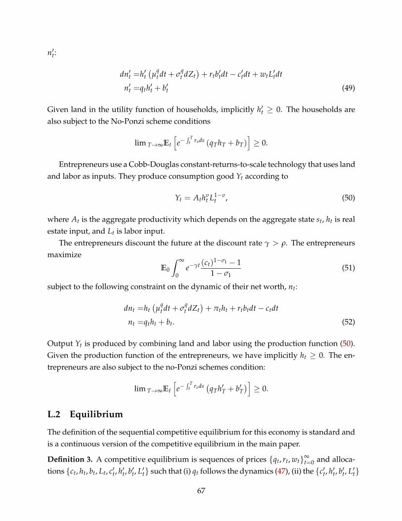
n′t:

dn′t =h′t(µ

qt dt + σ

qt dZt

)+ rtb′tdt− c′tdt + wtL′tdt

n′t =qth′t + b′t (49)

Given land in the utility function of households, implicitly h′t ≥ 0. The households arealso subject to the No-Ponzi scheme conditions

lim T→∞Et

[e−´ T

t rsds (qThT + bT)]≥ 0.

Entrepreneurs use a Cobb-Douglas constant-returns-to-scale technology that uses landand labor as inputs. They produce consumption good Yt according to

Yt = Athυt L1−υ

t , (50)

where At is the aggregate productivity which depends on the aggregate state st, ht is realestate input, and Lt is labor input.

The entrepreneurs discount the future at the discount rate γ > ρ. The entrepreneursmaximize

E0

ˆ ∞

0e−γt (ct)1−σ1 − 1

1− σ1(51)

subject to the following constraint on the dynamic of their net worth, nt:

dnt =ht(µ

qt dt + σ

qt dZt

)+ πtht + rtbtdt− ctdt

nt =qtht + bt. (52)

Output Yt is produced by combining land and labor using the production function (50).Given the production function of the entrepreneurs, we have implicitly ht ≥ 0. The en-trepreneurs are also subject to the no-Ponzi schemes condition:

lim T→∞Et

[e−´ T

t rsds (qTh′T + b′T)]≥ 0.

L.2 Equilibrium

The definition of the sequential competitive equilibrium for this economy is standard andis a continuous version of the competitive equilibrium in the main paper.

Definition 3. A competitive equilibrium is sequences of prices {qt, rt, wt}∞t=0 and alloca-

tions {ct, ht, bt, Lt, c′t, h′t, b′t, L′t} such that (i) qt follows the dynamics (47), (ii) the {c′t, h′t, b′t, L′t}

67

maximize (48) subject to the dynamic net worth constraint (49) and the no-Ponzi condi-tion and {ct, ht, bt, Lt} maximize (51) subject to dynamic net worth constraint (52) andthe no-Ponzi condition, and production technology (50) given {qt, rt, wt} and initial as-set holdings {h0, b0, h′0, b′0}; (iii) land, bond, labor, and good markets clear: ht + h′t = H,bt + b′t = 0, Lt = L′t, ct + c′t = Yt.

Let ωt denote the normalized financial wealth of the entrepreneurs

ωt =nt

qtH

and ω′t denote the normalized financial wealth of the households:

ω′t =n′t

qtH.

By the land and bond market clearing conditions, we have ω′t = 1−ωt in any competitiveequilibrium. Therefore in order to keep track of the normalized financial wealth distri-bution between the entrepreneurs and the households, (ωt, ω′t), in equilibrium, we onlyneed to keep track of ωt. To simplify the language, we use the term wealth distribution fornormalized financial wealth distribution.

Markov equilibrium is also a continuous version of Markov equilibrium in the mainpaper.

Definition 4. A Markov equilibrium is a competitive equilibrium in which prices and al-locations at time t, depend only on the wealth distribution at time t, ωt and the exogenousstate At.

This Markov equilibrium is the same as the Markov equilibria in Brunnermeier andSannikov (2014) and He and Krishnamurthy (2013). We can use the algorithms in their pa-pers to solve for the Markov equilibrium in our paper. However, there are two importantdifferences. First, because of persistent TFP shocks (instead of I.I.D. depreciation shocksto capital stock as in Brunnermeier and Sannikov (2014) or I.I.D. return shocks on divi-dend as in He and Krishnamurthy (2013)), in our Markov equilibrium, we need to keeptrack of both wealth distribution and the current exogenous shock. Second, we allow forgeneral utility functions, instead of linear or log utility functions as in Brunnermeier andSannikov (2014) and He and Krishnamurthy (2013).

68

M Multiple Production Technologies

In this section, we simplify our model in the main paper in the spirit of Brunnermeier andSannikov (2014) as well as Cordoba and Ripoll (2004b) and Kiyotaki and Moore (1997).We assume that the households do not have a preference for housing but have access toan inefficient production function

Y′ = Ahν′L1−ν′ (53)

with min(At) < A < max (At). Households maximize a lifetime utility function givenby

E0

∞

∑t=0

βt{(c′t)

1−σ2 − 11− σ2

− 1η(Lt)

η

}, (54)

where Lt is the hours of work (instead of L′t in the benchmark model). The budget con-straint of the households is

c′t + qt(h′t − h′t−1) + ptb′t ≤ b′t−1 + wt Lt + Y′t − wtL′t. (55)

Housing is no longer in the utility function of households, so we have to impose explicitly

h′t ≥ 0.

Given their land holding at time t, ht, the households choose labor demand L′t to max-imize profit

maxL′t

{Y′t − wtL′t

}subject to their production technology (53) if they produce. The first order condition withrespect to L′t implies

wt = (1− υ′)Ahυ′t (L′t)

−υ′ ,

i.e. L′t =((1−υ′)At

wt

) 1v′ h′t and profit

Y′t − wtL′t = π′th′t

where π′t = v′A((1−υ′)A

wt

) 1−vv is profit per unit of land for the households.

Definition 5. A competitive equilibrium is sequences of prices {pt, qt, wt}t,st and alloca-

tions{

ct, ht, bt, Lt, c′t, h′t, b′t, L′t, Lt

}t,st

such that (i){

c′t, h′t, b′t, L′t, Lt

}t,st

maximize (54) sub-

69

ject to the budget constraint (55), the production technology (53), h′t ≥ 0 and the No-Ponzi condition, and {ct, ht, bt, Lt}t,st maximize (51) subject to the entrepreneur’s budgetconstraint, production technology (50), and a collateral constraint, given {pt, qt, wt} andsome initial asset holdings

{h−1, b−1, h′−1, b′−1

}; (ii) land, bond, labor, and good markets

clear: ht + h′t = H, bt + b′t = 0, Lt + L′t = Lt, ct + c′t = Yt.

In the steady state, the entrepreneurs own the whole supply of land. Outside thesteady state, we can use the definition of Markov equilibrium and the associated solutionmethod as in the benchmark model in the main paper. The main difference between thesolution of this model and the benchmark model is that at the natural borrowing limitfor the entrepreneurs, i.e. ωt = 0, the households start producing using their inefficientproduction function. This puts a higher lower bound on the total output as well as landprice compared to when the households cannot produce as in the main paper.

70