Amirmasoud Kalantari-Dahaghi* and Shahab D. · PDF fileBiographical notes: Amirmasoud...
30
104 Int. J. Oil, Gas and Coal Technology, Vol. 4, No. 2, 2011 Copyright © 2011 Inderscience Enterprises Ltd. A new practical approach in modelling and simulation of shale gas reservoirs: application to New Albany Shale Amirmasoud Kalantari-Dahaghi* and Shahab D. Mohaghegh Department of Petroleum and Natural Gas Engineering, West Virginia University, Morgantown, West Virginia, 26506, USA E-mail: [email protected] E-mail: [email protected] *Corresponding author Abstract: The intent of this study is to reassess the potential of New Albany Shale formation using a novel and integrated workflow, which incorporates natural fracture system modeling with top-down intelligent reservoir modelling technique. Top-down, intelligent reservoir modeling technology integrates reservoir engineering analytical techniques with artificial intelligence and data mining in order to arrive at an empirical, cohesive and spatiotemporally calibrated full field model. The model is used to predict reservoir performance. Analytical reservoir engineering techniques used in the top-down modelling presented in this study include production decline analysis, type curve matching, single well history matching, volumetric reserve and recovery factor estimations are integrated with Voronoi graph theory, geostatistics, two-dimensional fuzzy pattern recognition, and discrete, data driven predictive modelling. The resulting full field top-down modeling is used to identify the distribution of the remaining reserves, sweet spots for infill locations, under-performer wells and also prediction of new well’s performance. [Received: April 25, 2010; Accepted: July 04, 2010] Keywords: shale gas; natural fracture system; fuzzy pattern recognition; FPR; intelligent reservoir model. Reference to this paper should be made as follows: Kalantari-Dahaghi, A. and Mohaghegh, S.D. (2011) ‘A new practical approach in modelling and simulation of shale gas reservoirs: application to New Albany Shale’, Int. J. Oil, Gas and Coal Technology, Vol. 4, No. 2, pp.104–133. Biographical notes: Amirmasoud Kalantari-Dahaghi received his MS in Petroleum and Natural Gas Engineering from West Virginia University in 2010. Currently, he is a PhD student in Petroleum and Natural Gas Engineering at West Virginia University. His current research interests include modelling and simulation of unconventional gas resources, CO 2 sequestration, and real time data analysis using artificial intelligence and data mining. S.D. Mohaghegh received his PhD in Petroleum and Natural Gas Engineering from Penn State University in 1991. He is currently a Professor at the Department of Petroleum and Natural Gas Engineering, West Virginia University. His current research interests include smart fields and application of intelligent systems in production optimisation and reservoir evaluation and engineering.
Transcript of Amirmasoud Kalantari-Dahaghi* and Shahab D. · PDF fileBiographical notes: Amirmasoud...

104 Int. J. Oil, Gas and Coal Technology, Vol. 4, No. 2, 2011
Copyright © 2011 Inderscience Enterprises Ltd.
A new practical approach in modelling and simulation of shale gas reservoirs: application to New Albany Shale
Amirmasoud Kalantari-Dahaghi* and Shahab D. Mohaghegh Department of Petroleum and Natural Gas Engineering, West Virginia University, Morgantown, West Virginia, 26506, USA E-mail: [email protected] E-mail: [email protected] *Corresponding author
Abstract: The intent of this study is to reassess the potential of New Albany Shale formation using a novel and integrated workflow, which incorporates natural fracture system modeling with top-down intelligent reservoir modelling technique. Top-down, intelligent reservoir modeling technology integrates reservoir engineering analytical techniques with artificial intelligence and data mining in order to arrive at an empirical, cohesive and spatiotemporally calibrated full field model. The model is used to predict reservoir performance. Analytical reservoir engineering techniques used in the top-down modelling presented in this study include production decline analysis, type curve matching, single well history matching, volumetric reserve and recovery factor estimations are integrated with Voronoi graph theory, geostatistics, two-dimensional fuzzy pattern recognition, and discrete, data driven predictive modelling. The resulting full field top-down modeling is used to identify the distribution of the remaining reserves, sweet spots for infill locations, under-performer wells and also prediction of new well’s performance. [Received: April 25, 2010; Accepted: July 04, 2010]
Keywords: shale gas; natural fracture system; fuzzy pattern recognition; FPR; intelligent reservoir model.
Reference to this paper should be made as follows: Kalantari-Dahaghi, A. and Mohaghegh, S.D. (2011) ‘A new practical approach in modelling and simulation of shale gas reservoirs: application to New Albany Shale’, Int. J. Oil, Gas and Coal Technology, Vol. 4, No. 2, pp.104–133.
Biographical notes: Amirmasoud Kalantari-Dahaghi received his MS in Petroleum and Natural Gas Engineering from West Virginia University in 2010. Currently, he is a PhD student in Petroleum and Natural Gas Engineering at West Virginia University. His current research interests include modelling and simulation of unconventional gas resources, CO2 sequestration, and real time data analysis using artificial intelligence and data mining.
S.D. Mohaghegh received his PhD in Petroleum and Natural Gas Engineering from Penn State University in 1991. He is currently a Professor at the Department of Petroleum and Natural Gas Engineering, West Virginia University. His current research interests include smart fields and application of intelligent systems in production optimisation and reservoir evaluation and engineering.

A new practical approach in modelling and simulation of shale gas reservoirs 105
1 Introduction
1.1 Unconventional reservoir reservoirs definition (Sondergeld et al., 2010)
Similar to conventional hydrocarbon systems, unconventional gas reservoirs are characterised by complex geological and petrophysical systems as well as heterogeneities – at all scales. However, unlike conventional reservoirs, unconventional gas reservoirs typically have very fine grain rock texture, exhibit gas storage and flow characteristics which are uniquely tied to nano-scale pore throat and pore size distribution and possess common organic and clay content that serve as gas sorption sites. Gas-shale reservoir pore structures are defined in terms of nanometres to micrometers, whereas most tight gas reservoirs are described at a micrometer or larger scale. Both gas-shale and tight gas systems have free gas stored within the pores of the rock matrix. Gas-shale differs in possessing the characteristic of gas adsorption on surface areas associated with organic content and clay. Bustin et al. (2008a, 2008b) states that the relative importance of adsorbed versus free gas varies as a function of the amount of organic matter present, pore size distribution, mineralogy, digenesis, rock texture and reservoir pressure and temperature. Gas shale reservoirs in the USA tend to be found within three depth ranges between 250 and 8,000 ft. The New Albany and Antrim shales, for example, have some 9,000 wells in the range of 250 ft. to 2,000 ft.
In the Appalachian basin shales and the Devonian and Lewis shales, there are about 20,000 wells from 3,000 ft. to 5,000 ft. Although the Barnett and Woodford shales are much deeper, the Caney and Fayetteville shales are from 2,000 ft. to 6,000 ft., with most of the reservoirs between 2,500 ft. and 4,500 ft. A good shale gas prospect has a shale thickness between 300 ft. and 600 ft. (Sondergeld et al., 2010).
Shale has such low permeability that it releases gas very slowly, which is why shale is the last major source of natural gas to be developed. Shale can hold a vast amount of natural gas. The most prolific shales are relatively flat, thick, and predictable, and the formations are so large that their wells will continue producing gas at a steady rate for decades.
Fractures are the key to good production. The more fractures in the shale around the wellbore, the faster the gas will be produced. Because of shale’s extremely low permeability, the best fracture treatments are those that expose as much of the shale as possible to the pressure drop that allows the gas to flow. The natural formation pressure of a large gas shale reservoir will decline only slightly over decades of production. Any pressure drop on individual wells is likely the result of fractures closing up, rather than depletion of the reservoir. The key to good shale gas production over time is having the proper distribution and placement of proppant to keep the fractures open.
Hydraulic fracture propagation is mainly controlled by combination of in situ stress, reservoir pressures, the rock matrix, and the natural fracture system. Therefore, the major concern in production from shale is the identification of hydraulic fracture growth and their interaction with the natural fracture system. So, identifying the natural fracture characteristics play an important role in successful hydraulic fracturing design.
1.2 New Albany Shale formation
The name New Albany Black Slate was originally proposed by Borden (1874) for brownish-black shale exposed along the Ohio River at New Albany, Floyd County,
106 A. Kalantari-Dahaghi and S.D. Mohaghegh
Indiana. This unit is currently designated the New Albany Shale. The New Albany consists of brownish-black, organic-rich and greenish-grey, organic-poor shale and is present in the subsurface throughout much of the Illinois Basin. The New Albany Shale formation occurs in Illinois, Indiana, and Kentucky, but to date gas production has been primarily from western Indiana and southwest Kentucky.
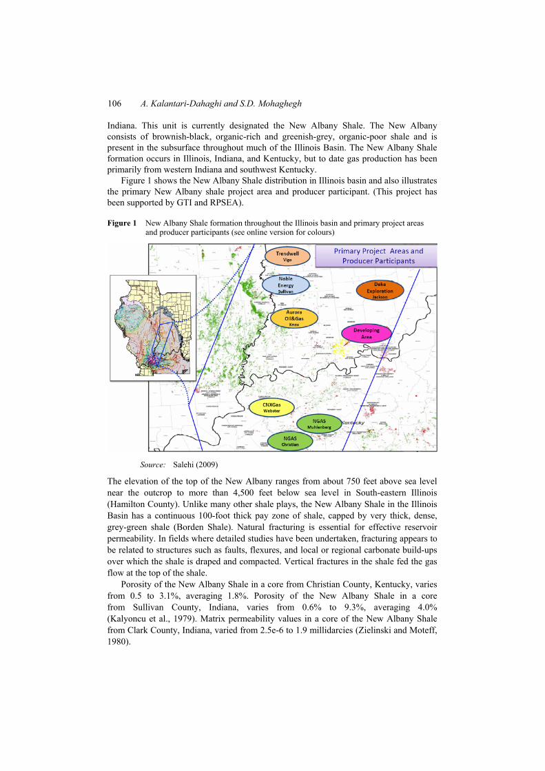
Figure 1 shows the New Albany Shale distribution in Illinois basin and also illustrates the primary New Albany shale project area and producer participant. (This project has been supported by GTI and RPSEA).
Figure 1 New Albany Shale formation throughout the Illinois basin and primary project areas and producer participants (see online version for colours)
Source: Salehi (2009)
The elevation of the top of the New Albany ranges from about 750 feet above sea level near the outcrop to more than 4,500 feet below sea level in South-eastern Illinois (Hamilton County). Unlike many other shale plays, the New Albany Shale in the Illinois Basin has a continuous 100-foot thick pay zone of shale, capped by very thick, dense, grey-green shale (Borden Shale). Natural fracturing is essential for effective reservoir permeability. In fields where detailed studies have been undertaken, fracturing appears to be related to structures such as faults, flexures, and local or regional carbonate build-ups over which the shale is draped and compacted. Vertical fractures in the shale fed the gas flow at the top of the shale.
Porosity of the New Albany Shale in a core from Christian County, Kentucky, varies from 0.5 to 3.1%, averaging 1.8%. Porosity of the New Albany Shale in a core from Sullivan County, Indiana, varies from 0.6% to 9.3%, averaging 4.0% (Kalyoncu et al., 1979). Matrix permeability values in a core of the New Albany Shale from Clark County, Indiana, varied from 2.5e-6 to 1.9 millidarcies (Zielinski and Moteff, 1980).

A new practical approach in modelling and simulation of shale gas reservoirs 107
The New Albany Shale is affected by complex faulting in Western Kentucky and adjacent parts of Illinois and Indiana. Elsewhere, less intense deformation has locally produced folds and faults that influence its elevation and thickness (Gas Research Institute, 1994).
The New Albany Shale in the Illinois Basin has promising gas production potential because of its high estimated gas content (86 TCF) and long history of production. Gas-in-place (GIP) measures from 8 bcfg/square mile to 20 or more bcfg/square mile, depending on locations and depths. Gas has been produced from the New Albany Shale since 1858, from at least 40 fields in Kentucky, 19 in Indiana, and one in Illinois. Production data are not publicly available, and none have been disclosed by operators to date. Only initial potential (IP) data are generally available. Measured IP values for New Albany Shale wells range from less than 10 to 4,500 MCFGPD and average 187 MCFGPD.
New Albany Shale gas is predominantly methane with significant and variable amounts of heavier hydrocarbons. It is very important to mention that water generally is not produced in western Kentucky, but is co-produced with gas in Indiana and along the Indiana and Kentucky border. (Gas Research Institute, 1994)
The New Albany Shale reservoir contains natural gas both as free gas in open pore space, and as adsorbed gas on interior clay and kerogen surfaces. Commercial production of gas from the New Albany Shale requires well stimulation that interconnects the well bore with the natural fracture system. Effective stimulation maintains permeability by introducing a proppant into the pressure-sensitive fractures near the well bore. Current stimulations are hydraulic-fracture treatments using nitrogen foam with a proppant; these treatments have replaced the older gelatinated nitroglycerine explosive shots.
The amount of organic carbon in the New Albany Shale is quite variable, ranging from near 0 weight% in greenish-grey beds to 25 weight% in brownish-black organic-rich beds (Gas Research Institute, 1994).
Characterising the relative conductivity of the fracture network and primary fracture are critical to evaluating stimulation performance. Because of the uncertainty in matrix permeability and network fracture spacing (i.e., complexity), it is difficult to find unique solutions when modelling production from unconventional gas reservoirs.
Gas desorption may not be a significant component in many moderate to deep shale-gas reservoirs, such as the New Albany, Barnett, Marcellus, and Haynesville Shales. Although adsorbed gas may comprise 40 to 50% of the total GIP, modelling suggests that gas desorption likely has a minor effect on well performance and desorption may add 5% to 15% to ultimate gas recovery (unlike CBM formation). Therefore, desorbed gas production is probably a minor component in economic development of many shale gas plays. Gas desorption can probably be ignored in many reservoir simulations, especially when evaluating initial well performance (first five years). In addition the ability to produce the adsorbed gas is limited because of the ultra-tight matrix rock, relatively high FBHP, and the desorption profile, which requires relatively low pressures throughout the matrix to initiate desorption of significant quantities of gas. Effectively producing this vast resource of desorbed gas may require another step change in our completion technology. Completions will require very low FBHP combined with extremely high conductivity fracture networks that can conduct gas with negligible pressure losses to effectively initiate desorption throughout large portions of the reservoir (Cipolla et al., 2009a, 2009b, 2009c).

108 A. Kalantari-Dahaghi and S.D. Mohaghegh
2 Methodology
It is difficult to find unique solutions when modelling production data in unconventional gas reservoirs. However, it may be sufficient to identify qualitative behaviours that can distinguish between key production mechanisms. Therefore, a new Integrated Workflow has been introduced and summarised in Figure 2.
Figure 2 General integrated for New Albany Shale reservoir modelling (see online version for colours)
Three main steps involved in this workflow including data gathering and preparation, performing natural fracture system modelling and simulation and completing top-down intelligent reservoir modelling. Each step has been explained in details in the following sections.
2.1 New Albany Shale natural fracture system modelling and simulation
The modelling of fluid flow through fractured formations can be based on deterministic, stochastic or fractal formulations of flow paths and matrix volumes. Deterministic models, however, are generally unable to effectively describe many naturally fractured formations with respect to the distributions of flow path length, flow path connectivity, and matrix block size and shape (Kalyoncu et al., 1979).
NFFLOWTM is a numerical model for naturally fractured gas reservoirs (developed by NETL/DOE) that permits the modelling of irregular flow paths mimicking the complex system of interconnected natural fractures in such reservoirs. This type of natural fracture reservoir simulation permits a more accurate and realistic representation

A new practical approach in modelling and simulation of shale gas reservoirs 109
of fractured porous media when modelling fluid flow compared to the traditional deterministic formulations. The NFFLOWTM simulator is a single-phase (dry-gas), two-dimensional numerical model that solves fluid flow equations in the matrix and fracture domains sequentially for wells located in a bounded naturally fractured reservoir. The mathematical model ‘decouples’ fluid flow in fractures and matrix, and solves a one-dimensional unsteady state flow problem in the matrix domain to compute the volumetric flow rates from matrix into fractures and wellbores (McKoy and Sams, 2006).
FRACGENTM, the fracture network generator (developed by NETL/DOE), implements four Boolean models of increasing complexity through a Monte Carlo process that samples fitted statistical distributions for various network attributes of each fracture set. Three models account for hierarchical relations among fracture sets, and two generate fracture swarming. Termination/intersection frequencies may be controlled implicitly or explicitly.
Since FRACGEN/NFFLOW simulator is single phase and does not consider the desorption process, water production and gas desorption are two important issues while using this simulator. As stated in introduction section, water generally is not produced in western Kentucky, which is our area of study, but is co-produced with gas in Indiana and along the Indiana and Kentucky border (Gas Research Institute, 1994).
Cipolla et al. (2009a, 2009b, 2009c) suggested desorbed gas production is probably a minor component in economic development of many shale gas plays and can possibly be ignored in many reservoir simulations, especially when evaluating initial well performance (first five years).
In this study, FRACGEN/NFFLOW is being used to model gas production from New Albany Shale.
Figure 3 Schematic showing outcrop fracture features of the New Albany Shale
Source: Zober et al. (2002)
New Albany Shale reservoir contains high-angled (vertical or nearly so) orthogonal natural fractures with non-uniform spacing that are open to unimpeded flow. The predominant fracture system is oriented east-west with spacing between joints estimated to average five feet based on outcrop studies (Figure 3) and production simulations.
110 A. Kalantari-Dahaghi and S.D. Mohaghegh
Based on this information, it was concluded that increases in performance could be achieved with a horizontally drilled well compared to a vertically drilled well in the same reservoir.
Fractures in a core of the New Albany Shale from the Energy Resources of Indiana No. 1 Phegley Farms Inc. well in Sullivan County, Indiana, were described by Kalyoncu et al. (1979). Twenty-one fractures were described over an interval of 104 feet. They were mainly vertical, but some had dips as low as 80 degrees. The strike of the fractures was predominantly northwest-southeast and a small secondary mode trended slightly to the north of east-west (Ault, 1990). Joint orientations in outcrops of the New Albany Shale in Indiana are parallel to this secondary east-west trend of fractures in the Phegley Farms core (Ault, 1990). Fractures in a core of the New Albany Shale from the Orbit No. 1 Clark well in Christian County, Kentucky, were described by Miller and Johnson (1979). Natural fractures were regular planar sub vertical features striking northwest-southeast. They generally were filled with calcite, or less commonly with pyrite, and had apertures as great as 3.0 millimetres (0.0098 ft.). In the vertical plane, these fractures were commonly continuous for 1 or 2 feet, succeeded by sub parallel fractures offset from each other at their terminations (Ault, 1990).
There is a decrease in fracture from the top of the New Albany Shale to the lower members. The Clegg Creek member is clearly contains the most fractures, both natural and induced. The Blocher member typically shows half the number of natural fractures when compared to the clegg creek. Therefore, the Clegg Creek member contains the most natural fractures with fracture frequency decreasing down section.
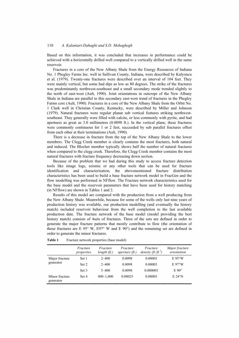
Because of the problem that we had during this study to access fracture detection tools like image logs, seismic or any other tools that can be used for fracture identification and characterisation, the abovementioned fracture distribution characteristics has been used to build a base fracture network model in FracGen and the flow modelling was performed in NFflow. The Fracture network characteristics used for the base model and the reservoir parameters that have been used for history matching (in NFflow) are shown in Tables 1 and 2.
Results of this model are compared with the production from a well producing from the New Albany Shale. Meanwhile, because for some of the wells only last nine years of production history was available, our production modelling (and eventually the history match) included reservoir behaviour from the well completion to the last available production date. The fracture network of the base model (model providing the best history match) consists of 4sets of fractures. Three of the sets are defined in order to generate the major fracture patterns that mostly contribute to flow (the orientation of those fractures are E 95° W, E97° W and E 90°) and the remaining set are defined in order to generate the minor fractures. Table 1 Fracture network properties (base model)
Fracture properties
Fracture length (ft.)
Fracture aperture (ft.)
Fracture density (ft./ft.2)
Major fracture orientation
Set 1 2–400 0.0098 0.00003 E 95°W
Set 2 2–400 0.0098 0.00003 E 97°W
Major fracture generator
Set 3 5–400 0.0098 0.000003 E 90°
Minor fracture generator
Set 4 400–1,000 0.00025 0.00003 E 24°N

A new practical approach in modelling and simulation of shale gas reservoirs 111
Generations of fracture sets are based on two different models. Model 1 generates randomly located fractures, although the connectivity controls can be used to produce various degrees of clustering, including unintended clustering. Model 2 generates fracture swarms (elongated clusters), whereby the swarms are randomly located and can overlap. Table 2 The input variable for single well history matching
Matrix permeability (md)
Matrix porosity (%) Initial pressure Thickness (ft.) A (acre)
0.0000822 5 700 100 320
The nine years production data of a well which is completed in New Albany Shale, Western Kentucky has been used to verify the built fracture network and perform history matching. The history matching result shows that the base model has significantly overestimated the production from this well. According to the well completion report (Kentucky Geological Survey) the initial rate after the stimulation at July 1973 is around146 MCF/day while the model results start at 127,830 MCF/day and declines to more than 70 MCF/day in about last nine years of production. To match the production from the New Albany Shale with the FracGen/NFflow simulator, sensitivity analysis was performed on fracture network properties (fracture aperture, length, and density) and reservoir properties (Pi, φm, Km, and h) in order to make the best estimation of NAS natural fracture network pattern.
2.1.1 Sensitivity analysis on reservoir and fracture properties
The objective of sensitivity analysis is to study the impact of different parameter and identify the factors that have the most contribution to flow. To investigate the effect of different reservoir and fracture property on flow behaviour, several studies were performed. The approach used for this analysis, starts by building the fracture network model based on the available information in literature (in FracGen). After performing the sensitivity analysis, the fracture network and reservoir properties of base model are tuned in order to match the observed production for each of the gas wells in New Albany Shale.
Figure 4 Sensitivity analysis on initial reservoir pressure (see online version for colours)
100
1000
0 20 40 60 80 100 120
Prod
uction
rate(M
SC/M
)
Time(Month)
qg(real) qg/m(Pi=410) qg/m(Pi=440)qg/m(Pi=470) qg/m(Pi=500) qg/m(Pi=530)
112 A. Kalantari-Dahaghi and S.D. Mohaghegh
Figure 5 Sensitivity analysis on matrix porosity (see online version for colours)
100
1000
0 20 40 60 80 100 120
Prod
uction
rate(M
CF/M
)
Time(Month)
qg(real) qg/m(phi=0.6) qg/m(phi=1.2)
qg/m(phi=1.8) qg/m(phi=2.4) qg/m(phi=3)
Figure 6 Sensitivity analysis on matrix permeability (see online version for colours)
100
1000
0 20 40 60 80 100 120
Prod
uction
rate(M
CF/M
)
Time(Month)
qg(real) qg/m(K=8.5e‐7) qg/m(K=1e‐6)
qg/m(K=2.5e‐6) qg/m(K=4e‐6) qg/m(K=5.5e‐6)
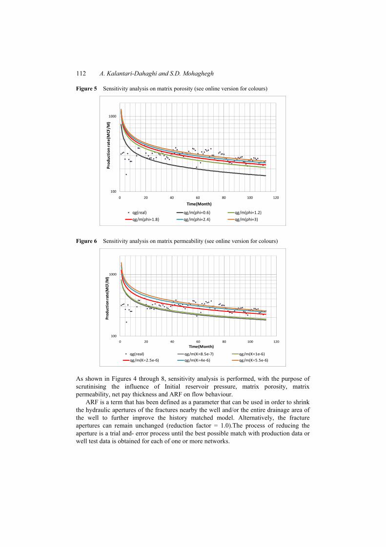
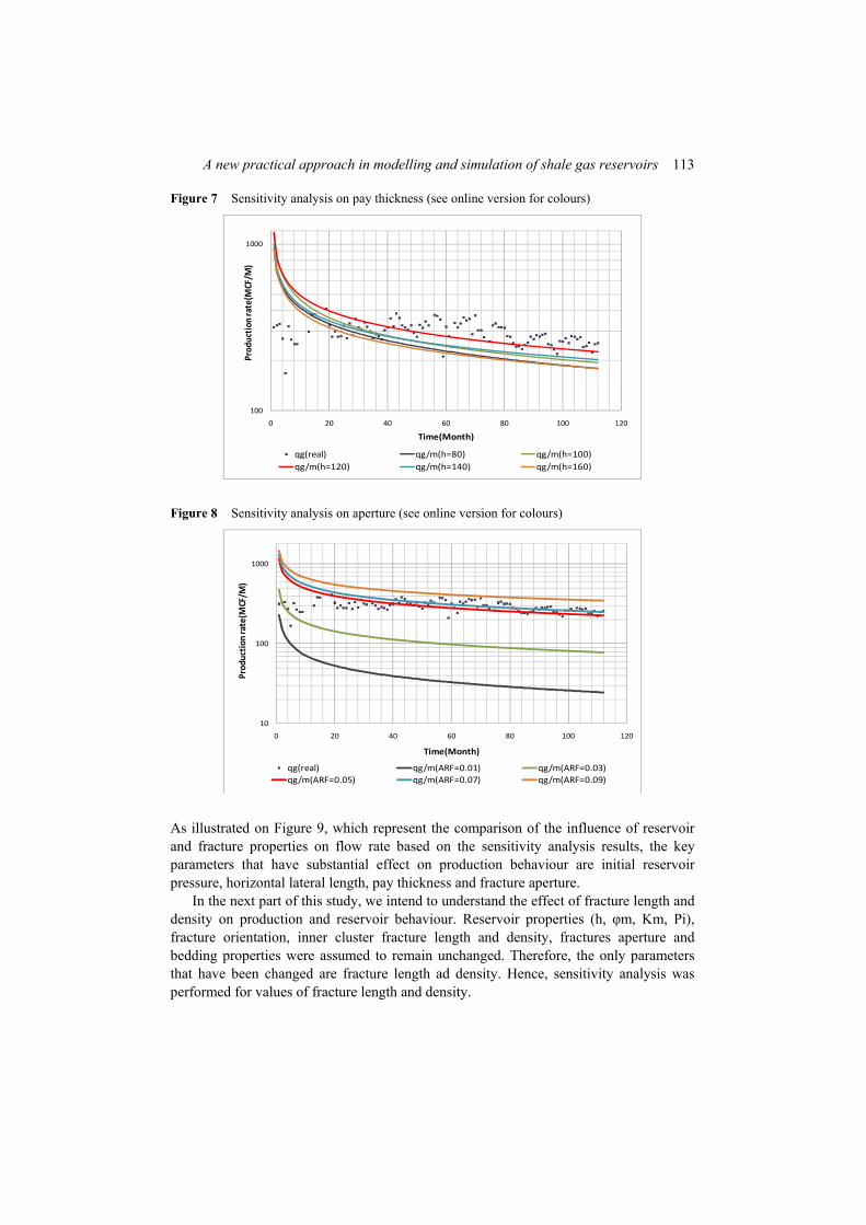
As shown in Figures 4 through 8, sensitivity analysis is performed, with the purpose of scrutinising the influence of Initial reservoir pressure, matrix porosity, matrix permeability, net pay thickness and ARF on flow behaviour.
ARF is a term that has been defined as a parameter that can be used in order to shrink the hydraulic apertures of the fractures nearby the well and/or the entire drainage area of the well to further improve the history matched model. Alternatively, the fracture apertures can remain unchanged (reduction factor = 1.0).The process of reducing the aperture is a trial and- error process until the best possible match with production data or well test data is obtained for each of one or more networks.
A new practical approach in modelling and simulation of shale gas reservoirs 113
Figure 7 Sensitivity analysis on pay thickness (see online version for colours)
100
1000
0 20 40 60 80 100 120
Prod
uction
rate(M
CF/M
)
Time(Month)
qg(real) qg/m(h=80) qg/m(h=100)qg/m(h=120) qg/m(h=140) qg/m(h=160)
Figure 8 Sensitivity analysis on aperture (see online version for colours)
10
100
1000
0 20 40 60 80 100 120
Prod
uction
rate(M
CF/M
)
Time(Month)
qg(real) qg/m(ARF=0.01) qg/m(ARF=0.03)qg/m(ARF=0.05) qg/m(ARF=0.07) qg/m(ARF=0.09)
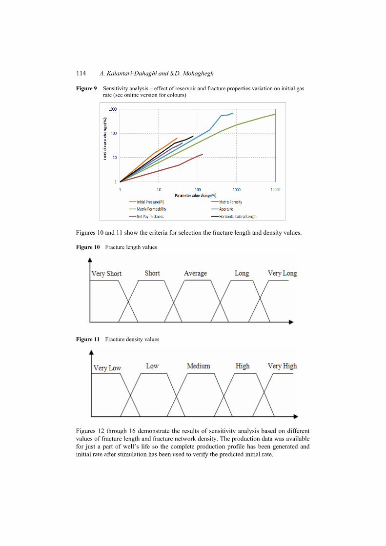
As illustrated on Figure 9, which represent the comparison of the influence of reservoir and fracture properties on flow rate based on the sensitivity analysis results, the key parameters that have substantial effect on production behaviour are initial reservoir pressure, horizontal lateral length, pay thickness and fracture aperture.
In the next part of this study, we intend to understand the effect of fracture length and density on production and reservoir behaviour. Reservoir properties (h, φm, Km, Pi), fracture orientation, inner cluster fracture length and density, fractures aperture and bedding properties were assumed to remain unchanged. Therefore, the only parameters that have been changed are fracture length ad density. Hence, sensitivity analysis was performed for values of fracture length and density.
114 A. Kalantari-Dahaghi and S.D. Mohaghegh
Figure 9 Sensitivity analysis – effect of reservoir and fracture properties variation on initial gas rate (see online version for colours)
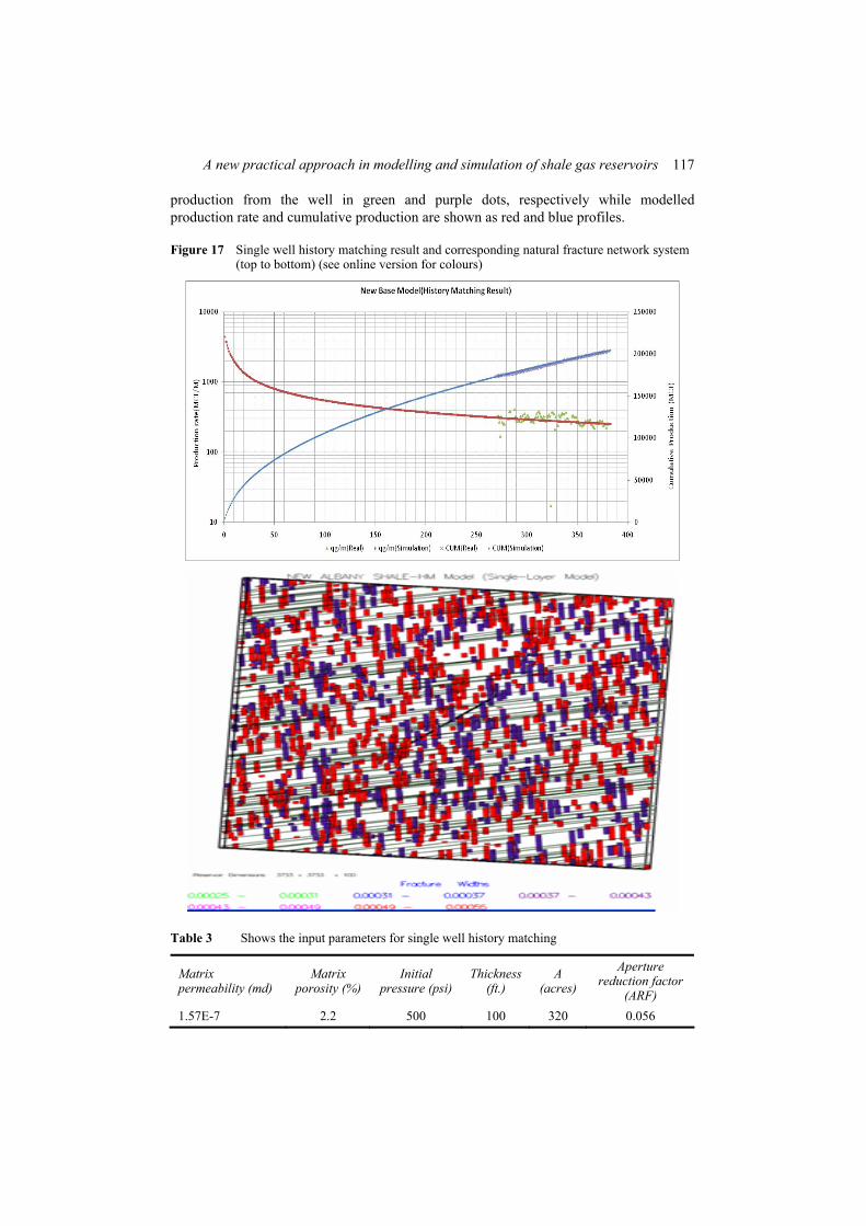
Figures 10 and 11 show the criteria for selection the fracture length and density values.
Figure 10 Fracture length values
Figure 11 Fracture density values
Figures 12 through 16 demonstrate the results of sensitivity analysis based on different values of fracture length and fracture network density. The production data was available for just a part of well’s life so the complete production profile has been generated and initial rate after stimulation has been used to verify the predicted initial rate.

A new practical approach in modelling and simulation of shale gas reservoirs 115
Figure 12 Sensitivity analysis results (very low fracture network density with variable length) (see online version for colours)
100
1000
10000
0 50 100 150 200 250 300 350 400
Productio
n rate(M
CF/M
)
Time(Month)
qg/m(Real) DVL‐LVL DVL‐LVS DVL‐LS DVL‐LA DVL‐LL
Figure 13 Sensitivity analysis results (low fracture network density with variable length) (see online version for colours)
100
1000
10000
0 50 100 150 200 250 300 350 400
Production
rate(MCF/M)
Time(Month)qg/m(Real) DL‐LVS DL‐LS DL‐LA DL‐LL DL‐LVL
Figure 14 Sensitivity analysis results (medium fracture network density with variable length) (see online version for colours)
100
1000
10000
0 50 100 150 200 250 300 350 400
Productio
n rate(M
CF/M
)
Time(Month)qg/m(Real) DM‐LVS DM‐LS DM‐LA DM‐LL DM‐LVL

116 A. Kalantari-Dahaghi and S.D. Mohaghegh
Figure 15 Sensitivity analysis results (high fracture network density with variable length) (see online version for colours)
100
1000
10000
0 50 100 150 200 250 300 350 400
Production
rate(MCF/M)
Time(Month)qg/m(Real) DH‐LVS DH‐LS DH‐LA DH‐LL DH‐LVL
Figure 16 Sensitivity analysis results (very high fracture network density with variable length) (see online version for colours)
100
1000
10000
0 50 100 150 200 250 300 350 400
Production
rate(MCF/M)
Time(Month)qg/m(Real) DVH‐LVS DVH‐LS DVH‐LA DVH‐LL DVH‐LVL
According to sensitivity analysis results, with increasing fracture length or fracture density the production will be increased. In the case that fracture length and/or density are low the fracture intersection will be decreased significantly, as a result some part of the reservoir will not be depleted, so the only way to put those parts of reservoir on production is performing some sort of stimulation (hydraulic fracturing).
2.1.2 History matched model
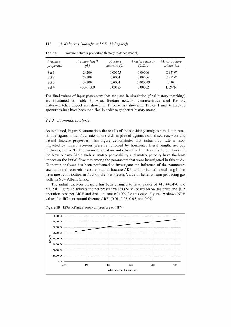
Upon completion of the sensitivity, analysis and careful study of the impact of different parameters on production a new set of parameters were identified. This new set was used in the model. The results of history matching and corresponding fracture network system shown in Figure 17.
According to the well completion report (Kentucky Geological Survey) the initial rate after the stimulation at July 1973 is 146 MCF/Day. The history matched model results in an initial production rate of 141 MCF/Day, which shows the reliability of fracture network and history matched model. Figure 17 shows production rates and cumulative
A new practical approach in modelling and simulation of shale gas reservoirs 117
production from the well in green and purple dots, respectively while modelled production rate and cumulative production are shown as red and blue profiles.
Figure 17 Single well history matching result and corresponding natural fracture network system (top to bottom) (see online version for colours)
Table 3 Shows the input parameters for single well history matching
Matrix permeability (md)
Matrix porosity (%)
Initial pressure (psi)
Thickness (ft.)
A (acres)
Aperture reduction factor
(ARF) 1.57E-7 2.2 500 100 320 0.056
118 A. Kalantari-Dahaghi and S.D. Mohaghegh
Table 4 Fracture network properties (history matched model)
Fracture properties
Fracture length (ft.)
Fracture aperture (ft.)
Fracture density (ft./ft.2)
Major fracture orientation
Set 1 2–200 0.00055 0.00006 E 95°W Set 2 2–200 0.0004 0.00006 E 97°W Set 3 5–200 0.0004 0.000009 E 90° Set 4 400–1,000 0.00025 0.00002 E 24°N
The final values of input parameters that are used in simulation (final history matching) are illustrated in Table 3. Also, fracture network characteristics used for the history-matched model are shown in Table 4. As shown in Tables 1 and 4, fracture aperture values have been modified in order to get better history match.
2.1.3 Economic analysis
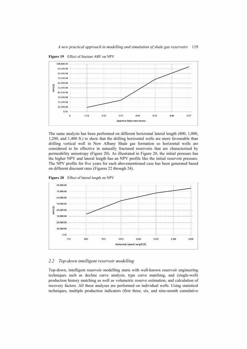
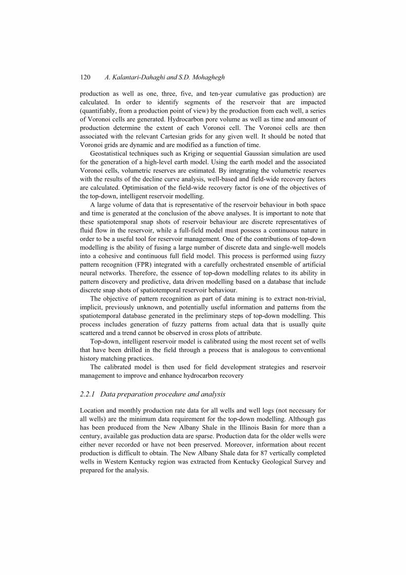
As explained, Figure 9 summarises the results of the sensitivity analysis simulation runs. In this figure, initial flow rate of the well is plotted against normalised reservoir and natural fracture properties. This figure demonstrates that initial flow rate is most impacted by initial reservoir pressure followed by horizontal lateral length, net pay thickness, and ARF. The parameters that are not related to the natural fracture network in the New Albany Shale such as matrix permeability and matrix porosity have the least impact on the initial flow rate among the parameters that were investigated in this study. Economic analyses has been performed to investigate the influence of the parameters such as initial reservoir pressure, natural fracture ARF, and horizontal lateral length that have most contribution in flow on the Net Present Value of benefits from producing gas wells in New Albany Shale.
The initial reservoir pressure has been changed to have values of 410,440,470 and 500 psi. Figure 18 reflects the net present values (NPV) based on $4 gas price and $0.5 operation cost per MCF and discount rate of 10% for this case. Figure 19 shows NPV values for different natural fracture ARF. (0.01, 0.03, 0.05, and 0.07)
Figure 18 Effect of initial reservoir pressure on NPV
A new practical approach in modelling and simulation of shale gas reservoirs 119
Figure 19 Effect of fracture ARF on NPV
The same analysis has been performed on different horizontal lateral length (800, 1,000, 1,200, and 1,400 ft.) to show that the drilling horizontal wells are more favourable than drilling vertical well in New Albany Shale gas formation so horizontal wells are considered to be effective in naturally fractured reservoirs that are characterised by permeability anisotropy (Figure 20). As illustrated in Figure 20, the initial pressure has the higher NPV and lateral length has an NPV profile like the initial reservoir pressure. The NPV profile for five years for each abovementioned case has been generated based on different discount rates (Figures 22 through 24).
Figure 20 Effect of lateral length on NPV
2.2 Top-down intelligent reservoir modelling
Top-down, intelligent reservoir modelling starts with well-known reservoir engineering techniques such as decline curve analysis, type curve matching, and (single-well) production history matching as well as volumetric reserve estimation, and calculation of recovery factors. All these analyses are performed on individual wells. Using statistical techniques, multiple production indicators (first three, six, and nine-month cumulative
120 A. Kalantari-Dahaghi and S.D. Mohaghegh
production as well as one, three, five, and ten-year cumulative gas production) are calculated. In order to identify segments of the reservoir that are impacted (quantifiably, from a production point of view) by the production from each well, a series of Voronoi cells are generated. Hydrocarbon pore volume as well as time and amount of production determine the extent of each Voronoi cell. The Voronoi cells are then associated with the relevant Cartesian grids for any given well. It should be noted that Voronoi grids are dynamic and are modified as a function of time.
Geostatistical techniques such as Kriging or sequential Gaussian simulation are used for the generation of a high-level earth model. Using the earth model and the associated Voronoi cells, volumetric reserves are estimated. By integrating the volumetric reserves with the results of the decline curve analysis, well-based and field-wide recovery factors are calculated. Optimisation of the field-wide recovery factor is one of the objectives of the top-down, intelligent reservoir modelling.
A large volume of data that is representative of the reservoir behaviour in both space and time is generated at the conclusion of the above analyses. It is important to note that these spatiotemporal snap shots of reservoir behaviour are discrete representatives of fluid flow in the reservoir, while a full-field model must possess a continuous nature in order to be a useful tool for reservoir management. One of the contributions of top-down modelling is the ability of fusing a large number of discrete data and single-well models into a cohesive and continuous full field model. This process is performed using fuzzy pattern recognition (FPR) integrated with a carefully orchestrated ensemble of artificial neural networks. Therefore, the essence of top-down modelling relates to its ability in pattern discovery and predictive, data driven modelling based on a database that include discrete snap shots of spatiotemporal reservoir behaviour.
The objective of pattern recognition as part of data mining is to extract non-trivial, implicit, previously unknown, and potentially useful information and patterns from the spatiotemporal database generated in the preliminary steps of top-down modelling. This process includes generation of fuzzy patterns from actual data that is usually quite scattered and a trend cannot be observed in cross plots of attribute.
Top-down, intelligent reservoir model is calibrated using the most recent set of wells that have been drilled in the field through a process that is analogous to conventional history matching practices.
The calibrated model is then used for field development strategies and reservoir management to improve and enhance hydrocarbon recovery
2.2.1 Data preparation procedure and analysis
Location and monthly production rate data for all wells and well logs (not necessary for all wells) are the minimum data requirement for the top-down modelling. Although gas has been produced from the New Albany Shale in the Illinois Basin for more than a century, available gas production data are sparse. Production data for the older wells were either never recorded or have not been preserved. Moreover, information about recent production is difficult to obtain. The New Albany Shale data for 87 vertically completed wells in Western Kentucky region was extracted from Kentucky Geological Survey and prepared for the analysis.

A new practical approach in modelling and simulation of shale gas reservoirs 121
Figure 21 Comparison the effect of different parameters on NPV (see online version for colours)
Figure 22 NPV profile for different Pi values (see online version for colours)
Because for some of the wells only last six to nine years of production history was available for the wells mentioned above, a unique natural fracture network modelling and simulation (FracGen/NFFlow) was performed in order to generate (through history matching) a relatively complete production profile for each of the 87 wells. The complete production profiles were generated using FracGen/NFFlow for the 87 wells based on 40, 80, 160 and 320 acres spacing. These production profiles were used to perform top-down intelligent reservoir modelling for the New Albany Shale gas reservoir. Figure 25 illustrates an example of generating the complete production profile for two of the NAS wells. In this figure, the green and black dots represent the actual production rates and cumulative production data collected from the Kentucky Geological Survey while the red and blue lines represent the history matched production rate and cumulative production profiles.
122 A. Kalantari-Dahaghi and S.D. Mohaghegh
Figure 23 NPV profile for different fracture aperture (see online version for colours)
Figure 24 NPV profile for different horizontal lateral length values (see online version for colours)
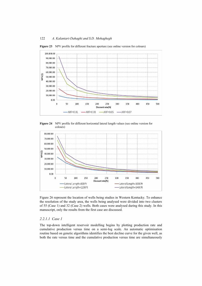
Figure 26 represent the location of wells being studies in Western Kentucky. To enhance the resolution of the study area, the wells being analysed were divided into two clusters of 55 (Case 1) and 32 (Case 2) wells. Both cases were analysed during this study. In this manuscript, only the results from the first case are discussed.
2.2.1.1 Case 1
The top-down intelligent reservoir modelling begins by plotting production rate and cumulative production versus time on a semi-log scale. An automatic optimisation routine based on genetic algorithms identifies the best decline curve for the given well, as both the rate versus time and the cumulative production versus time are simultaneously

A new practical approach in modelling and simulation of shale gas reservoirs 123
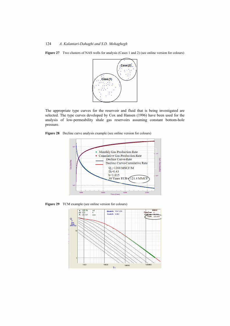
matched. This is demonstrated in Figure 28 for one of the NAS gas wells. Initial production rate Qi, initial decline rate Di, and hyperbolic exponent b are automatically identified. Additionally, the 30-year estimated ultimate recovery (EUR) is calculated. The information that results from the decline curve analysis is then passed to a type curve matching (TCM) procedure.
Figure 25 Simulation result examples for two history-matched New Albany Shale Gas wells (out of 87 wells) (see online version for colours)
Figure 26 Location of under-study area (see online version for colours)
124 A. Kalantari-Dahaghi and S.D. Mohaghegh
Figure 27 Two clusters of NAS wells for analysis (Cases 1 and 2) (see online version for colours)
The appropriate type curves for the reservoir and fluid that is being investigated are selected. The type curves developed by Cox and Hansen (1996) have been used for the analysis of low-permeability shale gas reservoirs assuming constant bottom-hole pressure.
Figure 28 Decline curve analysis example (see online version for colours)
Figure 29 TCM example (see online version for colours)

A new practical approach in modelling and simulation of shale gas reservoirs 125
Figure 30 History matching results in comparison with DCA for one of the wells (see online version for colours)
The TCM has been performed by plotting the production profile using decline curve analysis results rather than the actual production data in order to minimise the subjectivity of the TCM. Performing decline curve and type curve analyses is an iterative process. While following this procedure, we should always keep an eye on the 30 years EUR value calculated by these two methods as a controlling yardstick. These values should be reasonably close.
The third step of top-down modelling is numerical reservoir simulation using a single-well, radial numerical simulator. During history matching the production data, all of the information generated from the DCA and TCM is used to achieve an acceptable match.
Once the individual analysis(decline curve analysis, TCM) for all of the wells in the field is completed, the following information for all the wells in the field is available: initial flow rate (Qi), initial decline rate (Di), hyperbolic exponent (b), permeability (k), drainage area (A), fracture half length (Xf ), and 30 year EUR.
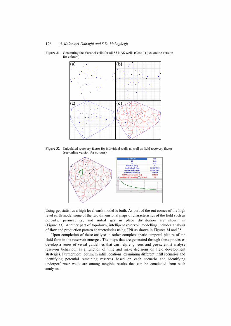
Figure 31 shows the well locations, followed by identification of boundary and the Voronoi grids for all the wells in the analysis for case 1. Using the results of decline curve analysis and volumetric reserve estimation, a well-based recovery factor is calculated for all wells, individually. A field-wide recovery factor is also calculated. Figure 32 illustrates the calculate recovery factory of 17.47% for one of the wells and field recovery factor of 23.58%.
Once the decline curve analysis and other steps mentioned above were completed, discrete, intelligent, predictive models are developed for the reservoir (production) attributes such as, first three, six, nine months and one, three, five, ten years of cumulative production, decline curve information (Qi, Di and b), EUR, Fracture half length, matrix and total porosity, matrix and total permeability, net pay thickness, Initial gas in place, and well recovery factor. These sets of discrete, intelligent models are then integrated using continuous FPR in order to arrive at a cohesive model of the reservoir as a whole.
126 A. Kalantari-Dahaghi and S.D. Mohaghegh
Figure 31 Generating the Voronoi cells for all 55 NAS wells (Case 1) (see online version for colours)
(a) (b)
(c) (d)
Figure 32 Calculated recovery factor for individual wells as well as field recovery factor (see online version for colours)
Using geostatistics a high level earth model is built. As part of the out comes of the high level earth model some of the two dimensional maps of characteristics of the field such as porosity, permeability, and initial gas in place distribution are shown in (Figure 33). Another part of top-down, intelligent reservoir modelling includes analysis of flow and production pattern characteristics using FPR as shown in Figures 34 and 35.
Upon completion of these analyses a rather complete spatio-temporal picture of the fluid flow in the reservoir emerges. The maps that are generated through these processes develop a series of visual guidelines that can help engineers and geo-scientist analyse reservoir behaviour as a function of time and make decisions on field development strategies. Furthermore, optimum infill locations, examining different infill scenarios and identifying potential remaining reserves based on each scenario and identifying underperformer wells are among tangible results that can be concluded from such analyses.

A new practical approach in modelling and simulation of shale gas reservoirs 127
Figure 33 Results of discrete predictive modelling showing the distribution of matrix porosity, and matrix permeability for the entire field (see online version for colours)
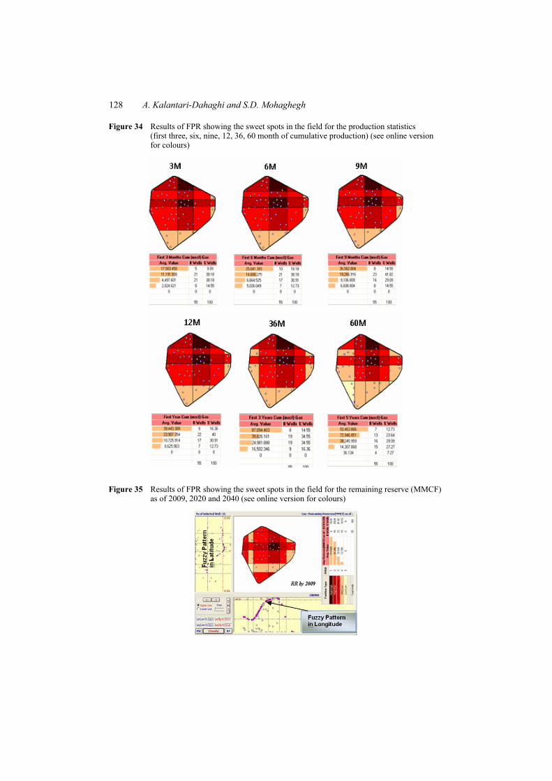
Figure 34 represents the cumulative production as a function of time and shows the most prolific area in from first three months of production to the 60th month of production.
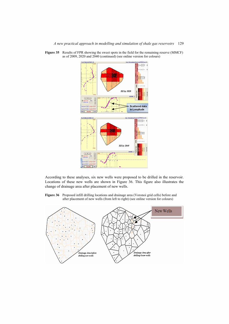
FPR technology includes generation of fuzzy patterns from actual data that is usually quite scattered and a trend cannot be observed in cross plots of attribute (such as remaining reserve) versus latitude and longitude. The remaining reserve as of year 2009, 2020 and 2040 has been shown in Figure 35. In the two dimensional maps (Figure 35) reservoir is delineated with relative reservoir quality index (RRQI) being the remaining reserves. The delineations shown in this figure are indicated by colours. Higher quality regions (regions with high values of Remaining Reserves) are shown in darker colours and as the average value of remaining reserves reduces in each region, the colour becomes increasingly lighter. The difference between these three figures shows the depletion in the reservoir and identifies the parts of the field that still have potential for more recovery.
Based on the results of predictive modelling and FPR, the best spots for drilling new wells were decided. The permeability is a key parameter that plays an important role in fluid production from the reservoir. Thereby having high initial production rate in the locations which have high permeability makes sense.
Another important factor while making decision about the infill drilling locations is remaining reserves. It defines the amount of the stored fluid in the reservoir. Having both the remaining reserves and permeability, results in high storage and flow capacity. Thus, the potential spots for infill drilling can be selected, based on these parameters. Although these two parameters have considerable effect on deciding the new well locations, other parameters such as production statistics (first three months to first five years of Cumulative production), forecasted EUR for 30 years, matrix porosity, initial gas in place and also fracture half length have been taken into account.
128 A. Kalantari-Dahaghi and S.D. Mohaghegh
Figure 34 Results of FPR showing the sweet spots in the field for the production statistics (first three, six, nine, 12, 36, 60 month of cumulative production) (see online version for colours)
Figure 35 Results of FPR showing the sweet spots in the field for the remaining reserve (MMCF) as of 2009, 2020 and 2040 (see online version for colours)
A new practical approach in modelling and simulation of shale gas reservoirs 129
Figure 35 Results of FPR showing the sweet spots in the field for the remaining reserve (MMCF) as of 2009, 2020 and 2040 (continued) (see online version for colours)
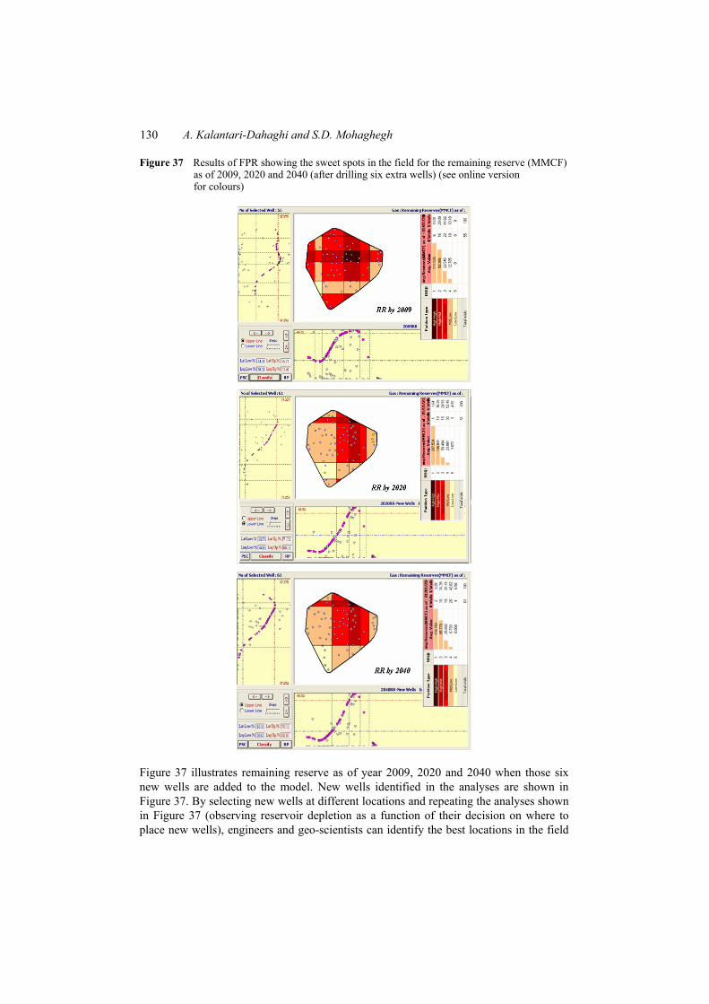
According to these analyses, six new wells were proposed to be drilled in the reservoir. Locations of these new wells are shown in Figure 36. This figure also illustrates the change of drainage area after placement of new wells.
Figure 36 Proposed infill drilling locations and drainage area (Voronoi grid cells) before and after placement of new wells (from left to right) (see online version for colours)
130 A. Kalantari-Dahaghi and S.D. Mohaghegh
Figure 37 Results of FPR showing the sweet spots in the field for the remaining reserve (MMCF) as of 2009, 2020 and 2040 (after drilling six extra wells) (see online version for colours)
Figure 37 illustrates remaining reserve as of year 2009, 2020 and 2040 when those six new wells are added to the model. New wells identified in the analyses are shown in Figure 37. By selecting new wells at different locations and repeating the analyses shown in Figure 37 (observing reservoir depletion as a function of their decision on where to place new wells), engineers and geo-scientists can identify the best locations in the field
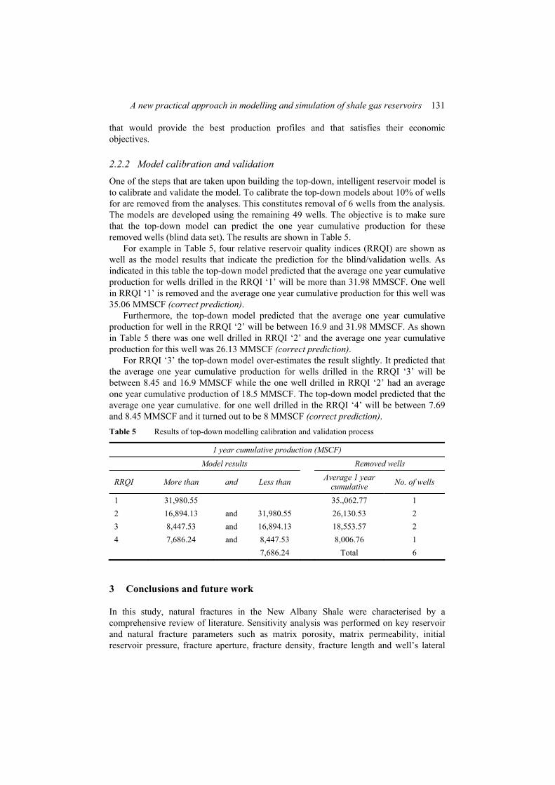
A new practical approach in modelling and simulation of shale gas reservoirs 131
that would provide the best production profiles and that satisfies their economic objectives.
2.2.2 Model calibration and validation
One of the steps that are taken upon building the top-down, intelligent reservoir model is to calibrate and validate the model. To calibrate the top-down models about 10% of wells for are removed from the analyses. This constitutes removal of 6 wells from the analysis. The models are developed using the remaining 49 wells. The objective is to make sure that the top-down model can predict the one year cumulative production for these removed wells (blind data set). The results are shown in Table 5.
For example in Table 5, four relative reservoir quality indices (RRQI) are shown as well as the model results that indicate the prediction for the blind/validation wells. As indicated in this table the top-down model predicted that the average one year cumulative production for wells drilled in the RRQI ‘1’ will be more than 31.98 MMSCF. One well in RRQI ‘1’ is removed and the average one year cumulative production for this well was 35.06 MMSCF (correct prediction).
Furthermore, the top-down model predicted that the average one year cumulative production for well in the RRQI ‘2’ will be between 16.9 and 31.98 MMSCF. As shown in Table 5 there was one well drilled in RRQI ‘2’ and the average one year cumulative production for this well was 26.13 MMSCF (correct prediction).
For RRQI ‘3’ the top-down model over-estimates the result slightly. It predicted that the average one year cumulative production for wells drilled in the RRQI ‘3’ will be between 8.45 and 16.9 MMSCF while the one well drilled in RRQI ‘2’ had an average one year cumulative production of 18.5 MMSCF. The top-down model predicted that the average one year cumulative. for one well drilled in the RRQI ‘4’ will be between 7.69 and 8.45 MMSCF and it turned out to be 8 MMSCF (correct prediction). Table 5 Results of top-down modelling calibration and validation process
1 year cumulative production (MSCF)
Model results Removed wells
RRQI More than and Less than Average 1 year cumulative No. of wells
1 31,980.55 35.,062.77 1 2 16,894.13 and 31,980.55 26,130.53 2 3 8,447.53 and 16,894.13 18,553.57 2 4 7,686.24 and 8,447.53 8,006.76 1 7,686.24 Total 6
3 Conclusions and future work
In this study, natural fractures in the New Albany Shale were characterised by a comprehensive review of literature. Sensitivity analysis was performed on key reservoir and natural fracture parameters such as matrix porosity, matrix permeability, initial reservoir pressure, fracture aperture, fracture density, fracture length and well’s lateral

132 A. Kalantari-Dahaghi and S.D. Mohaghegh
length .The orientation of natural fractures in New Albany Shale wells are EW and NNW-SSE and a minor ENE-SWS. Majority of natural fractures are vertical through there appears a minor set that dip between 55 to 75 degree.
A natural fracture network based on best available information and data was developed in FracGen. NFflow was used for fluid flow modelling based on the FracGen model. Reservoir characteristics and natural fracture properties were modified systematically until a reasonable history match was achieved for all the wells being studied.
The natural fracture model like any other geological model has a degree of uncertainty and can be updated by using additional information from fracture detection log, seismic and core analysis and any other tools that help to characterise fracture properties in order to building the more accurate model that represents the fracture network distribution of New Albany Shale.
A novel reservoir modelling technology has been applied to New Albany Shale. This relatively new modelling technology, top-down, intelligent reservoir modelling, incorporates artificial intelligent and data mining techniques such as data driven neural network modelling and FPR in conjunction with solid reservoir engineering analyses in order to combine single well analyses into a cohesive full field model.
Top-down intelligent reservoir modelling allows the reservoir engineer to plan and evaluate future development options for the reservoir and continuously updated the model that has been developed as new wells are drilled and more production data and well logs become available.
One of the most important advantages of top-down intelligent reservoir modelling is its ease of development. It is designed so that an engineer or a geologist will be able to comfortably develop a top-down model in a relatively short period of time with minimum amount of data (only monthly production data and some well logs are enough to start modelling). This new technique can be performed on the other types of shale and tight gas sand (unconventional resources) as well as conventional reservoirs (oil and gas).
Our studies have shown that intelligent top-down reservoir modelling holds much promise and can open new door for developing reservoir models using field measurement data. This new workflow can be performed on the other types of unconventional resources such as other shale plays and tight gas reservoirs.
Acknowledgements
Authors would like to acknowledge GTI and Research Partnership to Secure Energy for America (RPSEA) for partially funding this study and thank Intelligent Solutions, Inc. for supplying the IPDA and DOE-NETL for supplying FracGen/NFFlow software package.
References Ault, C.H. (1990) Directions and Characteristics of Jointing in the New Albany Shale (Devonian-
Mississippian) of South Eastern Indiana, Center for Applied Energy Research, IMMR89/201, Kentucky.
Borden, W.W. (1874) ‘Report of a geological survey of Clarke and Floyd Counties’, Indiana: Indiana Geological Survey Annual Report, Vol. 5, pp.133–189.

A new practical approach in modelling and simulation of shale gas reservoirs 133
Bustin, A.M.M., Bustin, R.M. and Cui, X. (2008a) Importance of Fabric on Production of Gas Shale, SPE 114167.
Bustin, M.R., Bustin, A., Ross, D., Chalmers, G., Murthy, V., Laxmi, C. and Cui, X. (2008b) Shale Gas Opportunities and Challenges. Search and Discovery Articles, AAPG Annual Convention, San Antonio, Texas.
Cipolla, C.L., Lolon, E.P. and Mayerhofer, M.J. (2009a) ‘Reservoir modeling and production evaluation in shale-gas reservoirs’, International Petroleum Technology Conference, Doha, Qatar.
Cipolla, C.L., Lolon, E.P., Erdle, J.C. and Rubin, B. (2009b) Reservoir Modeling in Shale-Gas Reservoirs, Charleston, West Virginia.
Cipolla, C.L., Lolon, E.P., Erdle, J.C. and Tathed, V. (2009c) Modeling Well Performance in Shale-Gas Reservoirs, Abu Dhabi, UAE.
Cox, D.O. and Hansen, J.T. (1996) ‘Advanced type curve analysis for low permeability gas reservoirs’, SPE 35595, SPE Gas Technology Symposium, 28 April–1 May, Calgary, Alberta, Canada.
Gas Research Institute (1994) Illinois Basin Consortium, Gas Potential of the New Albany Shale (Devonian and Mississippian) in the Illinois Basin.
Kalyoncu, R.S., Boyer, J.P. and Snyder, M.J. (1979) Characterization and Analysis of Devonian Shales as Related to Release of Gaseous Hydrocarbons, well P-1 Sullivan County, Indiana, Ohio.
http://kgsweb.uky.edu/DataSearching/OilGas/OGResults.asp?recno=63799&areatype=recno. McKoy, M.L. and Sams, W.N. (2006) Tight Gas Reservoir Simulation: Modeling Discrete
Irregular Strata-Bound Fracture Networks and Network Flow, Including Dynamic Recharge from the Matrix, DOE, Morgantown.
Miller, D.D., and Johnson, R.J.E. (1979) ‘Acoustic and mechanic analysis of a transverse anisotropy in shale’, Proceedings for Third Eastern Gas Shales Symposium, October, Morgantown, W. Va., Morgantown Energy Technology Center, U.S. Department of Energy, METC/SP-79/6, pp.527–542.
Salehi, I. (2009) New Albany Shale Project, Gas Technology Institute. Sondergeld, C.H., Newsham, K.E., Comisky, J.T., SPE and Rice, M.C. (2010) Petrophysical
Considerations in Evaluating and Producing Shale Gas Resources, SPE, 131768, Pittsburgh. Zielinski, R.E. and Moteff, J.D. (1980) Physical and Chemical Characterization of Devonian Gas
Shale: Quarterly Status Report, Monsanto Research Corporation, MLM-EGSP-TPR-Q-014, Miamisburg, Ohio.
Zober, M.D., Williamson, J.R. and Hill, D.G. (2002) A Comprehensive Reservoir Evaluation of a Shale Reservoirs, SPE 77469.