1

Ambient Seismic Noise

D. E McNamara1, R. P. Buland1, R. I. Boaz2, B. Weertman3 and T. Ahern3

1U.S. Geological Survey Golden CO, 2Boaz Consultancy,

3Incorporated Institutions for Seismology, Data Management Center

manuscript in preparation: SRL short note

Aug. 2005: PREPRINT v3.0

Correspondence to:

Daniel E. McNamaraUSGS1711 Illinois St.Golden, CO 80401(303) 273-8550 VOICE(303) 273-8600 FAXmcnamara@usgs.gov

Abstract

For earthquake-monitoring and detection purposes it is important to know the ambient

seismic nose levels experienced by a network of seismic stations. In this paper, we

present global ambient noise levels using 159 worldwide broadband stations within the

Global Seismographic Network (GSN) and the Advanced National Seismic System

(ANSS). To determine ambient noise conditions, we analyze the distribution of seismic

noise as a function of period and determine the highest probability power levels. While it

may be scientifically interesting to determine the absolute quietest noise levels achieved

by a network, we find that these low noise levels are generally very low probability

occurrences (1-3%) and do not closely track significantly higher probability (20-30%)

“ambient” noise conditions determined by the mode of the power distribution. In fact,

statistical mode noise levels are as much as 25dB above the minimum at higher

frequencies (1-10Hz) significant to earthquake monitoring.

2

Introduction

In this paper, we analyze ambient seismic noise levels, as defined by the highest

probability power levels at each period, for worldwide and U.S. broadband stations

within the global seismographic network (GSN) and the Advanced National Seismic

System (ANSS). Earth noise models have been used as baselines for evaluating seismic

station site characteristics and design, instrument design, and noise sources since the

published high and low seismic background displacement curves of Brune and Oliver

(1959) and Franti et al., (1962). Recently, the standard Peterson low noise model (LNM)

(Peterson, 1993) was updated by analyzing the absolute quietest conditions for stations

within the GSN during a one-year period in 2002-2003 (Berger et al., 2005). The original

Peterson LNM was constructed using minimum noise levels from representative quiet

periods at continental interior stations distributed around the world. Many seismic

stations are surrounded by urban areas and have considerably higher noise levels for

frequencies significant to earthquake monitoring (1-20Hz). This is the principle reason

that the noise levels of the LNM have such low probabilities of occurrence for stations

worldwide (Figure 1). For many stations such low levels of noise are unattainable

suggesting that for routine earthquake monitoring purposes a global noise threshold based

on higher probability noise levels is needed.

Noise Processing System and Methods

In June 2004, new software was made available to the seismology community that

allows users to evaluate the long-term seismic noise levels for any broadband seismic

data channel streaming into the buffer of uniform data (BUD) within the Incorporated

Research Institutions for Seismology (IRIS) data management system (DMS). BUD is the

IRIS DMS acronym for the online data cache from which the DMC distributes near-real

time miniSEED data holdings prior to formal archiving. The new noise processing

software uses a probability density function (PDF) to display the distribution of seismic

power spectral density (PSD). The algorithm and initial software were first developed at

the United States Geological Survey (USGS) as a part of the data and network quality

control (QC) system for the Advanced National Seismic System (ANSS) (McNamara and

3

Buland, 2004). Further development, supported by IRIS, allowed us to implement the

algorithm against the BUD dataset utilizing the QUACK framework. QUACK is a

software package under development at the IRIS DMC for analyzing real-time seismic

data flowing into the BUD (see http://www.iris.washington.edu/servlet/quackquery/).

The PDF noise analysis software is applied against the entire continuous data-stream

available within the BUD. There is no need to screen for system transients, earthquakes

or general data artifacts since they map into a background probability level. In fact,

examination of artifacts related to station operation and episodic cultural noise allows us

to estimate both the overall station quality and a baseline level of earth noise at each site.

The output of this noise analysis tool is useful for characterizing the current and past

performance of existing broadband sensors, for detecting operational problems within the

recording system, and for evaluating the overall quality of data for a particular station.

The advantages of this new approach include (1) providing an analytical view

representing the distribution noise levels rather than a simple absolute minimum, (2)

providing an assessment of the overall health of the instrument/station, and (3) providing

an assessment of the health of recording and telemetry systems.

Employing the system discussed above, which implements the algorithm used to

develop the USGS Albuquerque Seismological Laboratory (ASL) low noise model

(LNM; Peterson, 1993), we computed power spectral density (PSD) for 159 worldwide

seismic stations in the GSN and ANSS backbone networks (Table 1). In this algorithm,

hour-long, continuous, and overlapping (50%) time series segments are processed. Since

we are interested in the distribution of power levels from noise sources, there is no

removal of hourly segments with earthquakes, system transients, minor gaps and/or data

glitches. However, hourly segments with significant gaps, greater than 1 sec, are removed

from the statistical calculations. The instrument transfer function is then removed from

each segment, yielding ground acceleration (for easy comparison to the LNM). Each

hour-long time series is divided into 13 segments, each about 15 minutes long and

overlapping by 75%, with each segment processed by (1) removing the mean, (2)

removing the long period trend, (3) tapering using a 10% sine function, and (4)

transforming using an FFT algorithm (Bendat and Piersol, 1971). Segments are then

averaged to provide a PSD for each one-hour time series segment.

4

For each channel, raw frequency distributions are constructed by gathering individual

PSDs in the following manner (1) binning periods in 1/8 octave intervals, and (2) binning

power in 1 dB intervals. Each raw frequency distribution bin is then normalized by the

total number of PSDs to construct a Probability Density Function (PDF). The probability

of occurrence of a given power at a particular period for several stations in the GSN and

ANSS are plotted for direct comparison to the Peterson high and low noise models

(HNM, LNM; Figure 1). We also compute and plot the minimum, mode, and maximum

powers for each period bin. A wealth of seismic noise information can be obtained from

this statistical view of broadband seismic noise (Figure 1). For a more detailed discussion

of the noise processing methods see McNamara and Buland (2004).

GSN and ANSS PDFs

Our first observation is that noise power estimates are distributed over a wide range

of powers at all periods. Note that for all stations the maximum power (blue lines, Figure

1) is well above the HNM. Since we make no attempt to screen the seismic waveforms

for earthquakes and system transients, this high power region of the PDF is dominated by

low probability, yet high power occurrences of naturally occurring earthquakes, cultural

noise, data gaps, calibration pulses, mass re-centers and sensor glitches. Several PDF

noise sources, of this type, are labeled in figure 1. For a more detailed discussion of the

features observed in the PDFs see McNamara and Buland (2004).

The second observation we note in the PDFs is that the minimum powers (red lines,

Figure 1) are often near the LNM and very low probability (1-2%). We also observe

compression of the probability observations into a narrow power range suggesting that

each station can have a characteristic minimum level of background Earth noise. We also

note that the highest probability “ambient” noise levels, represented by the mode (black

line), are often affected by diurnal variations in the cultural noise band (0.1-1s, 1-10Hz)

and variations in the microsiesm peak (5-10s). At shorter periods, higher frequencies, the

mode and minimum are often divergent suggesting that the minimum does not represent

common station noise conditions. At periods greater than 10s, the mode and minimums

closely tack one another.

5

For example, at station LTX 3797, hours of data were used to generate the PDF

(Figure 1). As observed, the LTX minimum noise level has a probability of occurrence of

roughly 1%, suggesting that only 38 hours of data ever experienced such low levels of

noise. On the other hand, at periods of interest to the earthquake monitoring community

(0.1-1s, 1-10Hz), LTX noise levels were approximately 20dB higher than the minimum

for roughly 760 hours (see LTX mode figure 1) and roughly 30dB higher for an

additional 380 hours. The high frequencies at LTX are an extreme example of the

differences between the PDF minimums and modes however, it plainly illustrates our

point that “ambient” site conditions are better represented by the highest probability of

occurrence noise levels (i.e., PDF modes) (black lines Figure 1) than by the very low

probability minimum noise levels.

Ambient Earth Noise

In an effort to determine ambient Earth noise levels that are useful to the earthquake

monitoring and seismic network design community, we computed a PDF from the modes

of 159 GSN and ANSS BHZ channels (Figure 2). The plot shows the probabilistic

distribution of the highest probability occurrence noise levels (PDF modes) at 159

worldwide broadband seismic stations for periods from 0.1 to 100s. We also computed

additional statistics on the PDF modes (min, max, mean, median, mode) to illustrate the

distribution of the observations. The maximum noise level (dark blue line Figure 2) is

dominated by just a few, high noise, GSN stations located on islands (5-10s) and ANSS

stations with high levels of cultural noise (0.1-1s). For all periods considered, except at

the microseism peak (8sec), the maximum from this analysis, is higher than the Peterson

HNM. The minimum (red line Figure 2) at short periods (high frequencies) is lower than

the Peterson HNM but at periods greater than 10 seconds, the minimum is higher than the

Peterson LNM. However across the entire spectrum, it is evident from Figure 2 that, the

minimum has a very low probability of occurrence (1-2%). The minimum (red line figure

2) is dominated by one station in Antarctica, QSPA, at the higher frequencies (1.0-10Hz,

0.1-1s). Anderson et al. (2004) have determined that the high-frequency low power level

at QSPA is actually a spectral hole at 4Hz due too the thick surface ice layer, and does

not represent ambient noise conditions at the station. The median (pink line figure 2) and

6

mean (yellow line figure 2) noise levels are smooth and closely track one another at

power levels that range from 10-30dB above the LNM. The mode (white line figure 2) is

considerably less smooth due to the variation of noise levels across the networks but

tracks along approximately 10-20dB above the LNM. The mode represents the noise

conditions at roughly 10-20% of the stations analyzed in this study. The remaining

stations display a wide range of powers for periods from 0.1-100s.

For comparison, we have also plotted the mode low noise model (MLNM Figure 2)

from McNamara and Buland (2004). This noise model was constructed for earthquake

monitoring purposes from the minimum of the vertical component PDF modes of 65

broadband ANSS stations within the continental United States. It is interesting to note

that the minimum for stations restricted to the continental US (MLNM figure 2) is

generally 5-10dB higher than the minimum using global stations in this study (red line

Figure 2). The minimum noise level of all 159 stations (red line figure 2) closely tracks

the low powers of the Peterson LNM but are generally very low probability occurrences

(1-2%). For this reason the higher probability noise levels, represented by the median and

mode of the two networks give us an estimate of “ambient” Earth noise that is more

appropriate when designing seismic networks for earthquake monitoring.

Conclusions

We present a new approach to evaluate “ambient” noise levels at worldwide seismic

stations, based on the power spectral density methods used to generate the NLNM of

Peterson (1993) and statistical methods previously discussed in McNamara and Buland

(2004). The GSN and ANSS stations in our analysis exhibit considerable variations in

noise levels as a function of time of day, season, geography and sensor and installation

type. “Ambient” earth noise levels for global earthquake monitoring networks are

determined by analyzing the statistical distribution of the highest probability noise levels

(PDF modes) at GSN and ANSS stations throughout the world. The results of our noise

analysis are useful for characterizing the performance of existing GSN and ANSS

stations, for detecting operational problems, and should be relevant to choosing future

locations of ANSS backbone stations within the United States and optimizing the

distribution of regional network stations.

7

References

Anderson, K., Noise Analysis of the Global Seismographic Network station, QSPA:

Quiet Sector Antarctica, USGS Open File Report, in press, 2004.

Bendat, J.S. and A.G. Piersol (1971). Random data: analysis and measurement

procedures. John wiley and Sons, New York, 407p.

Berger, J., P. Davis, G. Ekstrom, Ambient Earth noise: a survey of the global

seismographic network, J. Geophys. Res., 109, 2005.

Brune, J.N , and J. Oliver (1959), The seismic noise of the Earth’s surface, Bull. Seism.

Soc. Am., 49, 349-353.

Franti, G.E, D.E. Willis and J.T. Wilson, The spectrum of seismic noise, Bull. Seism. Soc.

Am., 52, 1, 113-121, 1962.

McNamara, D.E. and R.P. Buland, Ambient Noise Levels in the Continental United

States, Bull. Seism. Soc. Am., 94,4,1517-1527, 2004.

Peterson, Observation and modeling of seismic background noise, U.S. Geol. Surv. Tech.

Rept., 93-322, 94p. 1993.

Figures

Figure 1: GSN and ANSS individual station PDF examples. BHZ.

Figure 2: PDF of individual GSN and ANSS station modes. BHZ.

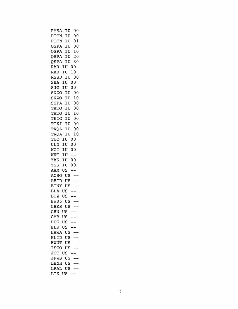
Table 1: Listing of stations used in this analysis.

8

9

(Figure 2: McNamara et al., 2004)

10

Table 1: Stations Used in Noise calculations

STA NET LOC

BJT IC 00ENH IC 00ENH IC 10HIA IC 00LSA IC 00LSA IC 10MDJ IC 00MDJ IC 10QIZ IC 00QIZ IC 01AAK II 00ARU II 00BFO II 00BORG II 00BORG II 10BRVK II 00CMLA II 00COCO II 20DGAR II 00DGAR II 10EFI II 00ESK II 00FFC II 00JTS II 00JTS II 10KDAK II 00KDAK II 10KIV II 00KURK II 00KWAJ II 00KWAJ II 10MBAR II 00MBAR II 10NNA II 00PALK II 00PALK II 10PFO II 00PFO II 10RPN II 00RPN II 10SACV II 00SACV II 10SUR II 00SUR II 10TAU II 00

11

WRAB II 00ADK IU 00ANMO IU 00ANMO IU 10ANTO IU 00BBSR IU 00BBSR IU 01BILL IU 00CASY IU 00CASY IU 10CCM IU 00COLA IU 00COLA IU 10COR IU 00CTAO IU 00DWPF IU 00GNI IU 00GRFO IU --GUMO IU 00GUMO IU 10HKT IU 00HRV IU --INCN IU 00INCN IU 10KBS IU 00KBS IU 10KIP IU 00KIP IU 10KMBO IU 00KMBO IU 10KONO IU 00KONO IU 10LSZ IU 00LSZ IU 10LVC IU 00LVC IU 10MA2 IU 00MAJO IU 00MBWA IU 10MIDW IU 00NWAO IU 00OTAV IU 00OTAV IU 10PAYG IU 00PAYG IU 10PET IU 00PMG IU 00PMG IU 10

12

PMSA IU 00PTCN IU 00PTCN IU 01QSPA IU 00QSPA IU 10QSPA IU 20QSPA IU 30RAR IU 00RAR IU 10RSSD IU 00SBA IU 00SJG IU 00SNZO IU 00SNZO IU 10SSPA IU 00TATO IU 00TATO IU 10TEIG IU 00TIXI IU 00TRQA IU 00TRQA IU 10TUC IU 00ULN IU 00WCI IU 00WVT IU --YAK IU 00YSS IU 00AAM US --ACSO US --AHID US --BINY US --BLA US --BOZ US --BW06 US --CBKS US --CBN US --CMB US --DUG US --ELK US --HAWA US --HLID US --HWUT US --ISCO US --JCT US --JFWS US --LBNH US --LRAL US --LTX US --

13

MCWV US --MIAR US --MNV US --MSO US --NCB US --NEW US --NHSC US --OCWA US --OXF US --RSSD US --SAO US --SDCO US --WCI US --WDC US --WMOK US --WUAZ US --WVOR US --WVT US --