Ambient Occlusion - Using Ray-tracing and Texture Blending
113
Ambient Occlusion - Using Ray-tracing and Texture Blending Ingvi Rafn Hafthorsson s041923 Kongens Lyngby 2007
Transcript of Ambient Occlusion - Using Ray-tracing and Texture Blending
Ambient Occlusion -Using Ray-tracing and
Texture Blending
Ingvi Rafn Hafthorssons041923
Kongens Lyngby 2007

Technical University of DenmarkInformatics and Mathematical ModellingBuilding 321, DK-2800 Kongens Lyngby, DenmarkPhone +45 45253351, Fax +45 [email protected]

Abstract
Ambient occlusion is the concept of shadows that accumulates at surfaces wherethe surface is partially hidden from the environment. The more the surface ishidden, the more ambient occlusion we have. The result is a subtle but realisticshadow effect on objects.
Ambient occlusion is implemented. To achieve this, existing methods are eval-uated and utilized. Ray-tracing is used for casting rays from surfaces. Theamount of rays that intersect the surrounding environment is used to find am-bient values. The more rays that hit, the more shadow we get at the surface weare working on.
We use textures for storing and displaying the ambient values. Overlapping tex-tures are implemented to eliminate visible seams at texture borders. A blendingbetween the textures is introduced. The blending factor is the normal vector atthe surface. We have three textures at the surface that each contain ambientvalues. To eliminate the possibility of having visible borders and seams betweentextures we suggest that the contribution of each texture will be values fromeach normal vector. The normal vector is normalized, and then we know that itsvalues squared will sum up to 1. This is according to the well known Pythagorastheorem. We then consider each of these values to be a percentage and we knowthat they sum up to be 100%. This allows for us to control the contribution ofeach ambient texture, assigning one texture color with one normal vector value.The result of this is a smooth blending of ambient values over the entire surfaceof curved objects.

ii
Preface
This thesis has been prepared at the Section of Computer Graphics, Depart-ment of Mathematical Modelling, IMM, at the Technical University of Denmark,DTU, in partial fulfillment of the requirements for the degree Master of Sciencein Engineering, M.Sc.Eng. The extent of the thesis is equivalent to 30 ETCScredits.
The thesis covers illumination of graphical models. In particular a shadow effect,called ambient occlusion. The reader is expected to have fundamental knowledgeof computer graphics, illumination models and shadows.
Lyngby, May 2007
Ingvi Rafn Hafthorsson

iv
Acknowledgements
First I want to thank my supervisors Niels Jørgen Christensen and Bent Dal-gaard Larsen for suggesting me to go in this direction. Bent I also thank foralways be willing to point me in the right direction when I got lost and alwaysbe willing to evaluate my progress, sometimes at unreasonable hours.
I thank my family for having faith in me. My mother for her biased comments(of course biased) and my sister for making the work in the last days possible.
I would like to thank my friend Hilmar Ingi Runarsson for valuable commentsand constructive critisims in the last days of work.
Last I thank my girlfriend Ragnheidur for her patience and understanding inthe final and most intense periods of the project work. Especially for alwaysbe willing to listen to my progress and thoughts no matter how much technicaldetails I was talking about.

vi
Contents
Abstract i
Preface iii
Acknowledgements v
1 Introduction 1
1.1 General Thoughts . . . . . . . . . . . . . . . . . . . . . . . . . . 1
1.2 Shadow Effects . . . . . . . . . . . . . . . . . . . . . . . . . . . . 3
1.3 Global Illumination . . . . . . . . . . . . . . . . . . . . . . . . . . 4
1.4 Ambient Occlusion . . . . . . . . . . . . . . . . . . . . . . . . . . 5
1.5 Contributions . . . . . . . . . . . . . . . . . . . . . . . . . . . . . 6
1.6 Thesis Overview . . . . . . . . . . . . . . . . . . . . . . . . . . . 7
2 Motivation and Goal 9
2.1 Motivation . . . . . . . . . . . . . . . . . . . . . . . . . . . . . . 9
viii CONTENTS
2.2 Goal . . . . . . . . . . . . . . . . . . . . . . . . . . . . . . . . . . 10
3 Ambient Occlusion in Practice 11
3.1 What is it . . . . . . . . . . . . . . . . . . . . . . . . . . . . . . . 11
3.2 When to use it . . . . . . . . . . . . . . . . . . . . . . . . . . . . 12
3.3 How is it implemented . . . . . . . . . . . . . . . . . . . . . . . . 13
4 Previous Work 15
4.1 Ambient Light Illumination Model . . . . . . . . . . . . . . . . . 15
4.2 The Model Refined . . . . . . . . . . . . . . . . . . . . . . . . . . 17
4.3 Advanced Ambient Occlusion . . . . . . . . . . . . . . . . . . . . 18
5 Occlusion Solution 21
5.1 General Approach . . . . . . . . . . . . . . . . . . . . . . . . . . 21
5.2 Using Vertices . . . . . . . . . . . . . . . . . . . . . . . . . . . . . 22
5.3 Using Textures . . . . . . . . . . . . . . . . . . . . . . . . . . . . 25
5.4 Blending Textures . . . . . . . . . . . . . . . . . . . . . . . . . . 27
5.5 Combining Textures . . . . . . . . . . . . . . . . . . . . . . . . . 28
6 Design 29
6.1 Import/Export . . . . . . . . . . . . . . . . . . . . . . . . . . . . 29
6.2 Data Representation . . . . . . . . . . . . . . . . . . . . . . . . . 30
6.3 Algorithms . . . . . . . . . . . . . . . . . . . . . . . . . . . . . . 30
6.4 Objects . . . . . . . . . . . . . . . . . . . . . . . . . . . . . . . . 32
CONTENTS ix
6.5 Final Structure . . . . . . . . . . . . . . . . . . . . . . . . . . . . 33
7 Implementation 35
7.1 Data Structure . . . . . . . . . . . . . . . . . . . . . . . . . . . . 35
7.2 Finding Adjacent Triangles . . . . . . . . . . . . . . . . . . . . . 41
7.3 Clustering Algorithm . . . . . . . . . . . . . . . . . . . . . . . . . 41
7.4 Finding Ambient Occlusion . . . . . . . . . . . . . . . . . . . . . 44
7.5 Texture Blending . . . . . . . . . . . . . . . . . . . . . . . . . . . 50
7.6 Texture Packing Algorithm . . . . . . . . . . . . . . . . . . . . . 50
7.7 User Input . . . . . . . . . . . . . . . . . . . . . . . . . . . . . . . 52
8 Testing 55
9 Results 59
10 Discussion 63
10.1 Summary . . . . . . . . . . . . . . . . . . . . . . . . . . . . . . . 63
10.2 Contributions . . . . . . . . . . . . . . . . . . . . . . . . . . . . . 64
11 Future Work 67
12 Conclusion 71
A Tools 75
A.1 COLLADA . . . . . . . . . . . . . . . . . . . . . . . . . . . . . . 75
A.2 COLLADA DOM . . . . . . . . . . . . . . . . . . . . . . . . . . . 76
x CONTENTS
A.3 Softimage XSI . . . . . . . . . . . . . . . . . . . . . . . . . . . . . 76
A.4 OpenGL and Cg . . . . . . . . . . . . . . . . . . . . . . . . . . . 77
B Screenshots 79
List of Figures
1.1 The importance of shadows. . . . . . . . . . . . . . . . . . . . . . 2
1.2 Ambient occlusion in a living room. . . . . . . . . . . . . . . . . 3
1.3 Hard shadows and soft shadows. . . . . . . . . . . . . . . . . . . 4
1.4 Ambient occlusion in a molecule model. . . . . . . . . . . . . . . 6
3.1 Self-occlusion and contact shadow. . . . . . . . . . . . . . . . . . 12
3.2 Worn gargoyle. . . . . . . . . . . . . . . . . . . . . . . . . . . . . 13
3.3 Ambient occlusion rays. . . . . . . . . . . . . . . . . . . . . . . . 14
4.1 Variables in the Ambient Light Illumination Model . . . . . . . . 16
5.1 Ambient occlusion found using the vertices. . . . . . . . . . . . . 23
5.2 Ambient occlusion using textures. . . . . . . . . . . . . . . . . . . 25
6.1 UML class diagram. . . . . . . . . . . . . . . . . . . . . . . . . . 34
xii LIST OF FIGURES
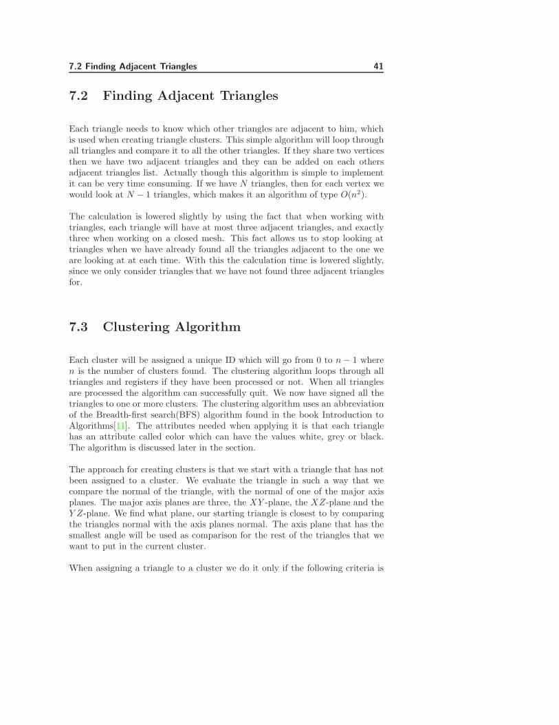
7.1 Cluster and the comparing plane. . . . . . . . . . . . . . . . . . . 42
7.2 Cluster mapped to 2D. . . . . . . . . . . . . . . . . . . . . . . . . 43
7.3 Regular clusters and overlapping clusters. . . . . . . . . . . . . . 44
7.4 Cluster patches. . . . . . . . . . . . . . . . . . . . . . . . . . . . . 45
7.5 Different number of rays. . . . . . . . . . . . . . . . . . . . . . . 46
7.6 Distance effect for rays. . . . . . . . . . . . . . . . . . . . . . . . 47
7.7 Cosine distribution for rays. . . . . . . . . . . . . . . . . . . . . . 47
7.8 Distance attenuation. . . . . . . . . . . . . . . . . . . . . . . . . . 49
7.9 Texture blending using normal vectors. . . . . . . . . . . . . . . . 51
7.10 Packed texture. . . . . . . . . . . . . . . . . . . . . . . . . . . . . 52
7.11 The object in the packed texture. . . . . . . . . . . . . . . . . . . 53
8.1 Scene 1 - Cornell Box. . . . . . . . . . . . . . . . . . . . . . . . . 56
8.2 Scene 2 - Comparison. . . . . . . . . . . . . . . . . . . . . . . . . 57
8.3 Scene 3 - Texture Blending. . . . . . . . . . . . . . . . . . . . . . 58
8.4 Scene 4 - Utah Teapot. . . . . . . . . . . . . . . . . . . . . . . . . 58
9.1 Clustering problem. . . . . . . . . . . . . . . . . . . . . . . . . . 60
9.2 The teapot problem. . . . . . . . . . . . . . . . . . . . . . . . . . 61
10.1 Ambient occlusion comparison. . . . . . . . . . . . . . . . . . . . 64
12.1 Cornell box scene. . . . . . . . . . . . . . . . . . . . . . . . . . . 72
B.1 Scene 1. . . . . . . . . . . . . . . . . . . . . . . . . . . . . . . . . 80
LIST OF FIGURES xiii
B.2 Scene 1. . . . . . . . . . . . . . . . . . . . . . . . . . . . . . . . . 81
B.3 Scene 1. . . . . . . . . . . . . . . . . . . . . . . . . . . . . . . . . 82
B.4 Scene 1. . . . . . . . . . . . . . . . . . . . . . . . . . . . . . . . . 83
B.5 Scene 2. . . . . . . . . . . . . . . . . . . . . . . . . . . . . . . . . 84
B.6 Scene 2. . . . . . . . . . . . . . . . . . . . . . . . . . . . . . . . . 85
B.7 Scene 2. . . . . . . . . . . . . . . . . . . . . . . . . . . . . . . . . 86
B.8 Scene 2. . . . . . . . . . . . . . . . . . . . . . . . . . . . . . . . . 87
B.9 Scene 2. . . . . . . . . . . . . . . . . . . . . . . . . . . . . . . . . 88
B.10 Scene 2. . . . . . . . . . . . . . . . . . . . . . . . . . . . . . . . . 89
B.11 Scene 3. . . . . . . . . . . . . . . . . . . . . . . . . . . . . . . . . 90
B.12 Scene 3. . . . . . . . . . . . . . . . . . . . . . . . . . . . . . . . . 90
B.13 Scene 3. . . . . . . . . . . . . . . . . . . . . . . . . . . . . . . . . 91
B.14 Scene 3. . . . . . . . . . . . . . . . . . . . . . . . . . . . . . . . . 91
B.15 Scene 4. . . . . . . . . . . . . . . . . . . . . . . . . . . . . . . . . 92
B.16 Scene 4. . . . . . . . . . . . . . . . . . . . . . . . . . . . . . . . . 92
B.17 Scene 4. . . . . . . . . . . . . . . . . . . . . . . . . . . . . . . . . 93

xiv LIST OF FIGURES
Chapter 1
Introduction
1.1 General Thoughts
There are many reasons why we want to model the world around us. There canbe educational purposes, recreational or simply curiosity. By creating modelswe present the possibility of exploring objects that would be beyond our reachin real life. For example we can model molecules and simulate their behavior,and thereby explore something that would be hard to do otherwise. There isalso the possibility of modeling a fictional world that has only the restraints ofthe imagination of its creator.
If we want to simulate the real world we have to consider physics and try toincorporate them in our model. This can be the physics of how light transportsand reflects or how objects interact with each other. It could also be a globaleffect like the earths gravity pull. The possibilities are endless. It would beimpossible to simulate exactly the real life physics in to a virtual world, thecomputer power needed for that would be enormous. Instead it is common tosimulate physics by “cheating” and trying to consider only things that affect theviewer and not consider anything that the viewer can’t see anyway. Anotherway of trying to simulate the real world is by simplifying the physics and therebysimulate something that looks realistic to a viewer but does in fact not obey therules of physics.
2 Introduction
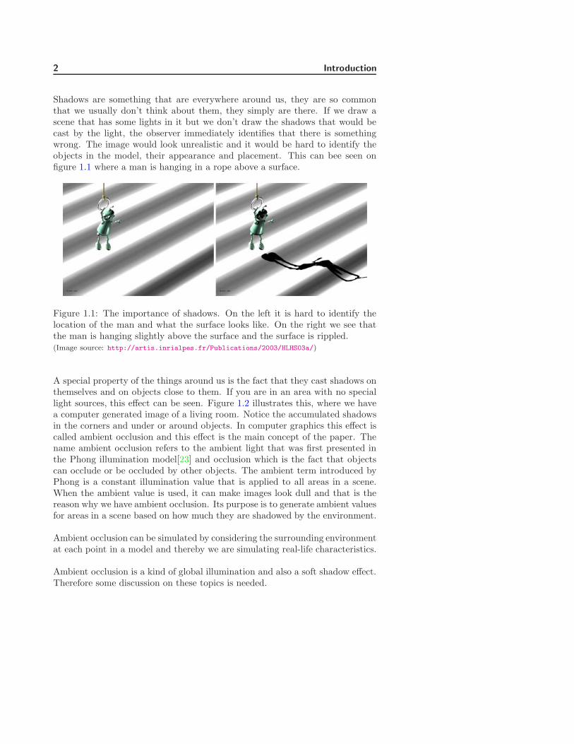
Shadows are something that are everywhere around us, they are so commonthat we usually don’t think about them, they simply are there. If we draw ascene that has some lights in it but we don’t draw the shadows that would becast by the light, the observer immediately identifies that there is somethingwrong. The image would look unrealistic and it would be hard to identify theobjects in the model, their appearance and placement. This can bee seen onfigure 1.1 where a man is hanging in a rope above a surface.
Figure 1.1: The importance of shadows. On the left it is hard to identify thelocation of the man and what the surface looks like. On the right we see thatthe man is hanging slightly above the surface and the surface is rippled.(Image source: http://artis.inrialpes.fr/Publications/2003/HLHS03a/)
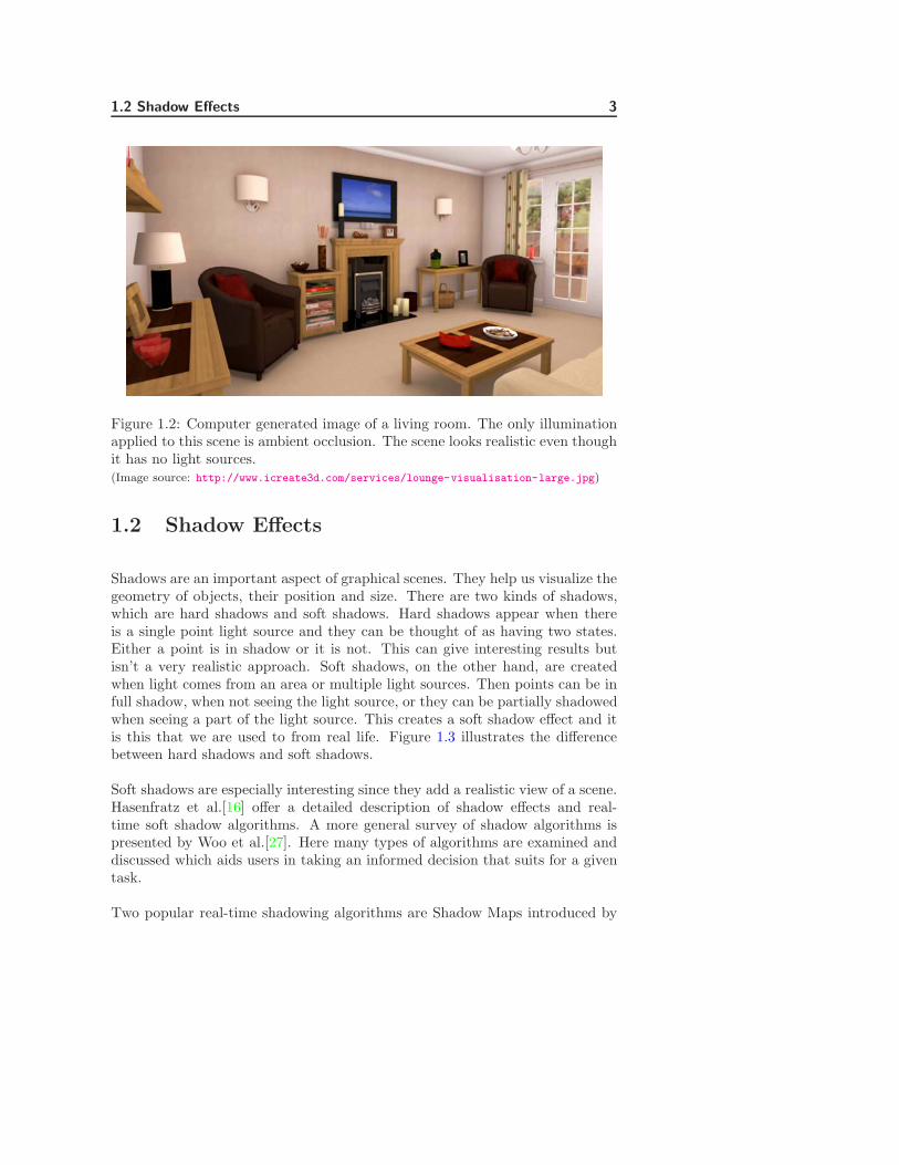
A special property of the things around us is the fact that they cast shadows onthemselves and on objects close to them. If you are in an area with no speciallight sources, this effect can be seen. Figure 1.2 illustrates this, where we havea computer generated image of a living room. Notice the accumulated shadowsin the corners and under or around objects. In computer graphics this effect iscalled ambient occlusion and this effect is the main concept of the paper. Thename ambient occlusion refers to the ambient light that was first presented inthe Phong illumination model[23] and occlusion which is the fact that objectscan occlude or be occluded by other objects. The ambient term introduced byPhong is a constant illumination value that is applied to all areas in a scene.When the ambient value is used, it can make images look dull and that is thereason why we have ambient occlusion. Its purpose is to generate ambient valuesfor areas in a scene based on how much they are shadowed by the environment.
Ambient occlusion can be simulated by considering the surrounding environmentat each point in a model and thereby we are simulating real-life characteristics.
Ambient occlusion is a kind of global illumination and also a soft shadow effect.Therefore some discussion on these topics is needed.
1.2 Shadow Effects 3
Figure 1.2: Computer generated image of a living room. The only illuminationapplied to this scene is ambient occlusion. The scene looks realistic even thoughit has no light sources.(Image source: http://www.icreate3d.com/services/lounge-visualisation-large.jpg)
1.2 Shadow Effects
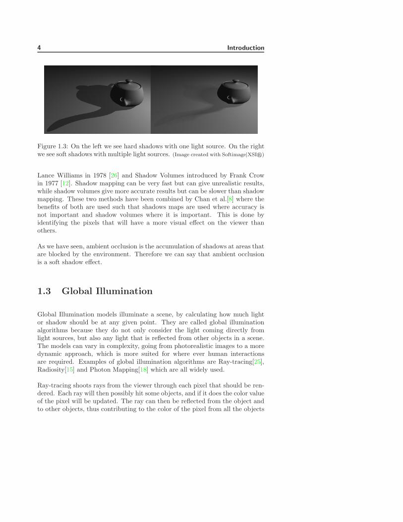
Shadows are an important aspect of graphical scenes. They help us visualize thegeometry of objects, their position and size. There are two kinds of shadows,which are hard shadows and soft shadows. Hard shadows appear when thereis a single point light source and they can be thought of as having two states.Either a point is in shadow or it is not. This can give interesting results butisn’t a very realistic approach. Soft shadows, on the other hand, are createdwhen light comes from an area or multiple light sources. Then points can be infull shadow, when not seeing the light source, or they can be partially shadowedwhen seeing a part of the light source. This creates a soft shadow effect and itis this that we are used to from real life. Figure 1.3 illustrates the differencebetween hard shadows and soft shadows.
Soft shadows are especially interesting since they add a realistic view of a scene.Hasenfratz et al.[16] offer a detailed description of shadow effects and real-time soft shadow algorithms. A more general survey of shadow algorithms ispresented by Woo et al.[27]. Here many types of algorithms are examined anddiscussed which aids users in taking an informed decision that suits for a giventask.
Two popular real-time shadowing algorithms are Shadow Maps introduced by
4 Introduction
Figure 1.3: On the left we see hard shadows with one light source. On the rightwe see soft shadows with multiple light sources. (Image created with Softimage|XSI)
Lance Williams in 1978 [26] and Shadow Volumes introduced by Frank Crowin 1977 [12]. Shadow mapping can be very fast but can give unrealistic results,while shadow volumes give more accurate results but can be slower than shadowmapping. These two methods have been combined by Chan et al.[8] where thebenefits of both are used such that shadows maps are used where accuracy isnot important and shadow volumes where it is important. This is done byidentifying the pixels that will have a more visual effect on the viewer thanothers.
As we have seen, ambient occlusion is the accumulation of shadows at areas thatare blocked by the environment. Therefore we can say that ambient occlusionis a soft shadow effect.
1.3 Global Illumination
Global Illumination models illuminate a scene, by calculating how much lightor shadow should be at any given point. They are called global illuminationalgorithms because they do not only consider the light coming directly fromlight sources, but also any light that is reflected from other objects in a scene.The models can vary in complexity, going from photorealistic images to a moredynamic approach, which is more suited for where ever human interactionsare required. Examples of global illumination algorithms are Ray-tracing[25],Radiosity[15] and Photon Mapping[18] which are all widely used.
Ray-tracing shoots rays from the viewer through each pixel that should be ren-dered. Each ray will then possibly hit some objects, and if it does the color valueof the pixel will be updated. The ray can then be reflected from the object andto other objects, thus contributing to the color of the pixel from all the objects

1.4 Ambient Occlusion 5
it has bounced off.
Radiosity is based on splitting the scene into patches and then a form factor isfound for each pair of patches, indicating how much the patches are visible toone another. The form factors are then used in rendering equations that lead tohow much each patch will be lit and then we have the whole scene illuminated.
In Photon Mapping, photons are sent out into the scene from a light source.When a photon intersects the scene, the point of intersection is stored alongwith the photons directions and energy. This information is stored in a photonmap. The photon can then be reflected back into the scene. This is usuallya preprocess step and then at rendering time, the photon map can be usedto modify the illumination at each point in the scene when using for exampleray-tracing.
We can think of ambient occlusion as a simple kind of global illumination algo-rithm, since it considers the surrounding environment but does not consider anylight sources. Remember that typically, global illumination models consider alllight sources and also light bouncing from other surfaces. Ambient occlusion isa relatively new method and has been gaining a lot of favor in the gaming andmovie industry and is now being used extensively.
1.4 Ambient Occlusion
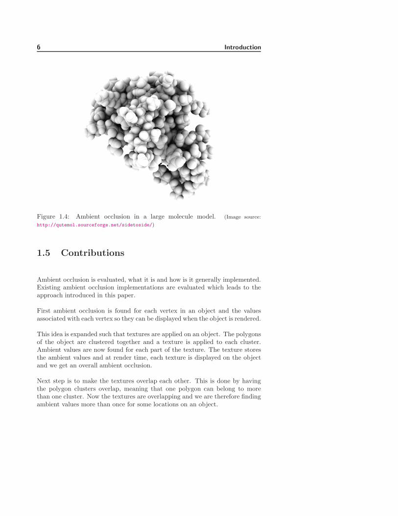
It is best to describe what ambient occlusion is by imagining a real-life circum-stances. A good example is the shadows that appear in corners of a room. It is ashadow that objects cast on itself or on objects that are close to them, and thiseffect is the main concept in the report. Figure 1.4 shows a complex computergenerated molecule with ambient occlusion shadows as the only illuminationapplied to it. Notice that the depth of the image is clear, we instantly identifythe structure of the object.
Details about ambient occlusion can be found in chapter 3 where general thoughtsabout why and when to use it and how it is implemented are discussed. Theorigins of ambient occlusion is discussed in chapter 4 along with a discussionon how it has evolved and some advanced ambient occlusion implementations.This finally leads to a discussion of the solution for ambient occlusion presentedin this paper which can be found in chapter 5.
6 Introduction
Figure 1.4: Ambient occlusion in a large molecule model. (Image source:
http://qutemol.sourceforge.net/sidetoside/)
1.5 Contributions
Ambient occlusion is evaluated, what it is and how is it generally implemented.Existing ambient occlusion implementations are evaluated which leads to theapproach introduced in this paper.
First ambient occlusion is found for each vertex in an object and the valuesassociated with each vertex so they can be displayed when the object is rendered.
This idea is expanded such that textures are applied on an object. The polygonsof the object are clustered together and a texture is applied to each cluster.Ambient values are now found for each part of the texture. The texture storesthe ambient values and at render time, each texture is displayed on the objectand we get an overall ambient occlusion.
Next step is to make the textures overlap each other. This is done by havingthe polygon clusters overlap, meaning that one polygon can belong to morethan one cluster. Now the textures are overlapping and we are therefore findingambient values more than once for some locations on an object.

1.6 Thesis Overview 7
This leads to us going to blend between the ambient values in an effort toget a smooth looking ambient occlusion. The blending will be done by usingthe values of the normal vectors as to how much each ambient value will con-tribute to the final color for each texture. Overlapping textures and blendingbetween them using the normal vectors has not been implemented before, to myknowledge. Details about how this is done is discussed in details in chapter 7 -Implementation.
The main contribution is to create textures that contain ambientvalues, make them overlap each other and blend between them usingthe normal vectors at each point as the blending factor.
We have many textures for complex objects and therefore we will create a textureatlas from all the cluster textures, to lower texture memory needed. A textureatlas is one texture that contains many small independent textures.
1.6 Thesis Overview
In chapter 2 there is a discussion about why we would want to implementambient occlusion, along with the goal that we want to achieve.
Chapters 3, 4 and 5 cover details about ambient occlusion in general, the prede-cessor of ambient occlusion, existing implementations and the proposed solutionpresented in this paper.
Chapters 6 and 7 cover the design and implementation details.
In chapters 8 and 9 the testing of the algorithm is discussed which is followedby results discussion.
The general idea of ambient occlusion and the path that was taken in this reportis discussed in chapter 10.
In chapter 11 there is a talk about extensions and improvements of the imple-mentation.
Finally in chapter 12 we conclude the thesis.

8 Introduction
Chapter 2
Motivation and Goal
2.1 Motivation
Generating visually pleasing graphical images can be a difficult task. We needto consider many factors to gain the result that is needed, often using a complexglobal illumination model to achieve this. This can be a time consuming task.
Objects and scenes need to look realistic, at least that much it will let theobserver feel like it possesses real-life characteristics. This can be achieved inmany ways e.g. by passing objects through an illumination model algorithmwhich calculates light and shadows for any given point, taking into consideration,existing lights and other things that affect the scene.
When complex objects are in equally distributed light, such as regular daylight,they will cast shadows on parts of themselves. Some parts will be less visibleto the surrounding environment and will therefore not get as much illuminationas others, thus being in more shadow. As mentioned earlier this effect is calledambient occlusion, and can be seen in figures 1.2 and 1.4.
If we have a static object, an object with no moving internal parts, then it is welldesirable to think of these shadows as constant. Meaning that no matter thesurrounding objects or lights, these shadows will always be the same. Of course
10 Motivation and Goal
the surrounding light will have an effect, but these shadows are still there.
The motivation would be to create a simple to use algorithm that finds ambientocclusion in objects and stores it in a convenient way. Then the ambient occlu-sion values can be accessed fast and be used again and again. This is thought ofas a preprocessing step, meaning that the algorithm should be used on objects,the output stored and used later for rendering. Possibly in real-time rendering.
2.2 Goal
The main objective will be to generate a natural looking illumination. Mainlythe shadow effect, called ambient occlusion, which are the shadows that accu-mulate on locations on objects that are occluded by the surrounding geometry.There will be a discussion about how this has been implemented before whichwill lead to the method introduced in this report.
Chapter 3
Ambient Occlusion in Practice
In order to implement ambient occlusion, we first need to discuss what it is,in what circumstances we benefit from using it, and how it is generally imple-mented.
3.1 What is it
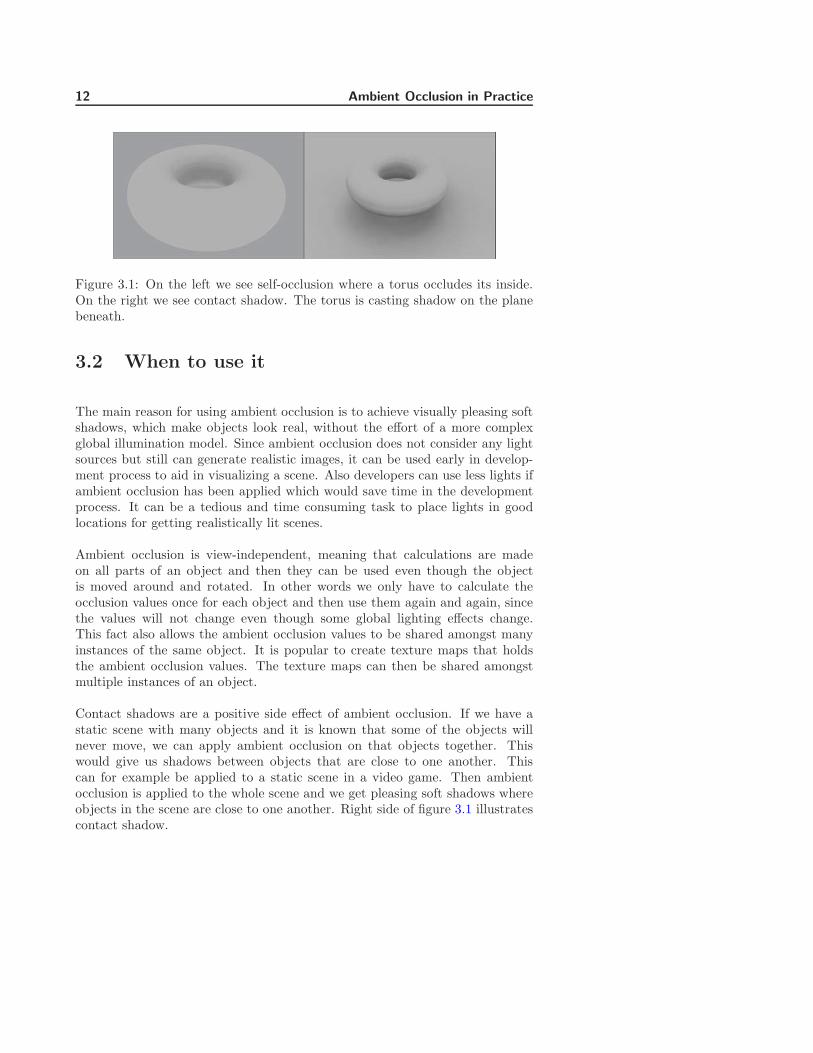
One special property of the things in the environment around us is the fact thatthey cast shadows on themselves or other things close to them. This property isbest described by imagining the shadows that accumulates in corners of roomsor the shadow on the ground beneath an object such as a car. When objectscast shadows on themselves it is called self-occlusion but when casting shadowson the surrounding environment it is called contact shadows. Contact shadowsare a positive side-effect of ambient occlusion, since generally it is designed tohandle only self-occlusion. Self-occlusion and contact shadows are illustrated infigure 3.1.
Ambient occlusion is the shadows that accumulates on places of objects, whichare not fully visible to the environment. Figures 1.2 and 1.4 in chapter 1 bothcatch the visual effects of ambient occlusion.
12 Ambient Occlusion in Practice
Figure 3.1: On the left we see self-occlusion where a torus occludes its inside.On the right we see contact shadow. The torus is casting shadow on the planebeneath.
3.2 When to use it
The main reason for using ambient occlusion is to achieve visually pleasing softshadows, which make objects look real, without the effort of a more complexglobal illumination model. Since ambient occlusion does not consider any lightsources but still can generate realistic images, it can be used early in develop-ment process to aid in visualizing a scene. Also developers can use less lights ifambient occlusion has been applied which would save time in the developmentprocess. It can be a tedious and time consuming task to place lights in goodlocations for getting realistically lit scenes.
Ambient occlusion is view-independent, meaning that calculations are madeon all parts of an object and then they can be used even though the objectis moved around and rotated. In other words we only have to calculate theocclusion values once for each object and then use them again and again, sincethe values will not change even though some global lighting effects change.This fact also allows the ambient occlusion values to be shared amongst manyinstances of the same object. It is popular to create texture maps that holdsthe ambient occlusion values. The texture maps can then be shared amongstmultiple instances of an object.
Contact shadows are a positive side effect of ambient occlusion. If we have astatic scene with many objects and it is known that some of the objects willnever move, we can apply ambient occlusion on that objects together. Thiswould give us shadows between objects that are close to one another. Thiscan for example be applied to a static scene in a video game. Then ambientocclusion is applied to the whole scene and we get pleasing soft shadows whereobjects in the scene are close to one another. Right side of figure 3.1 illustratescontact shadow.
3.3 How is it implemented 13
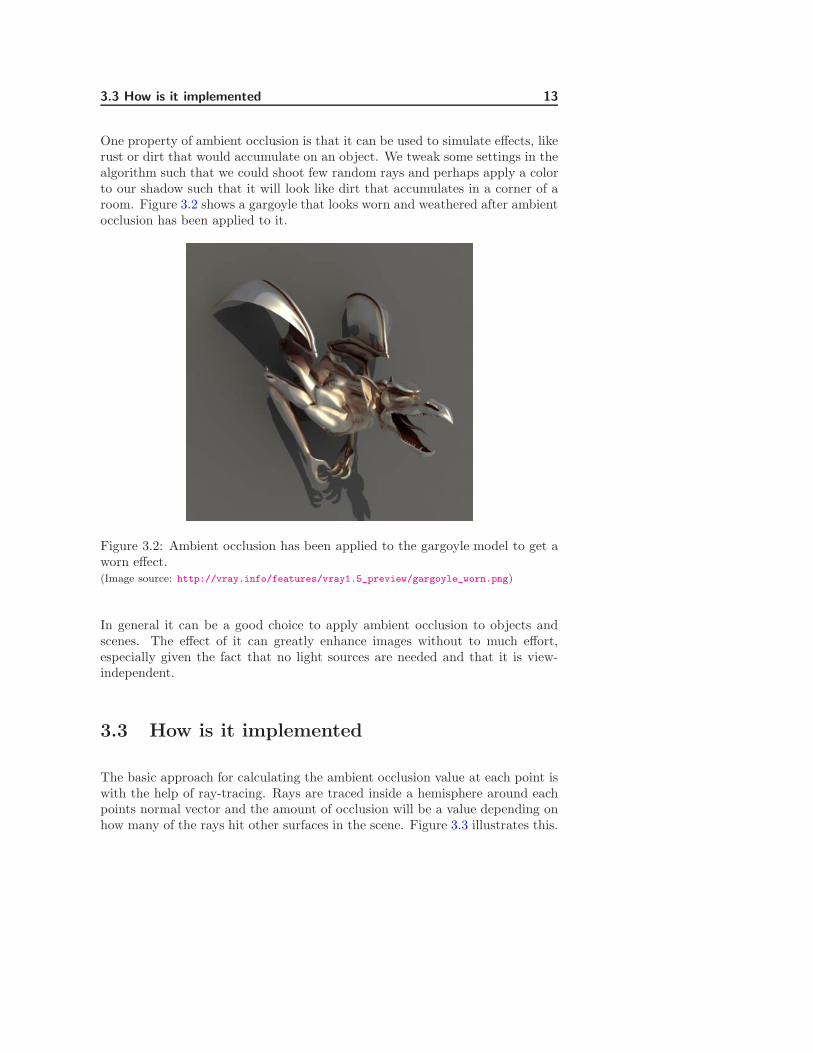
One property of ambient occlusion is that it can be used to simulate effects, likerust or dirt that would accumulate on an object. We tweak some settings in thealgorithm such that we could shoot few random rays and perhaps apply a colorto our shadow such that it will look like dirt that accumulates in a corner of aroom. Figure 3.2 shows a gargoyle that looks worn and weathered after ambientocclusion has been applied to it.
Figure 3.2: Ambient occlusion has been applied to the gargoyle model to get aworn effect.(Image source: http://vray.info/features/vray1.5_preview/gargoyle_worn.png)
In general it can be a good choice to apply ambient occlusion to objects andscenes. The effect of it can greatly enhance images without to much effort,especially given the fact that no light sources are needed and that it is view-independent.
3.3 How is it implemented
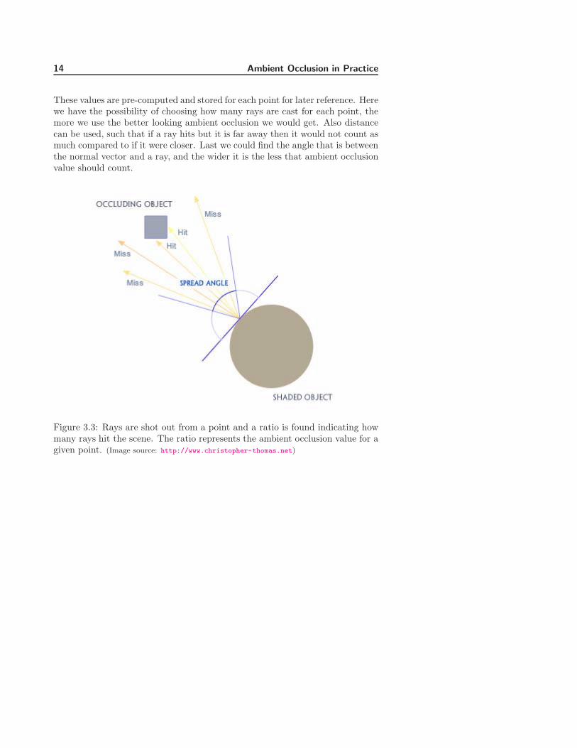
The basic approach for calculating the ambient occlusion value at each point iswith the help of ray-tracing. Rays are traced inside a hemisphere around eachpoints normal vector and the amount of occlusion will be a value depending onhow many of the rays hit other surfaces in the scene. Figure 3.3 illustrates this.
14 Ambient Occlusion in Practice
These values are pre-computed and stored for each point for later reference. Herewe have the possibility of choosing how many rays are cast for each point, themore we use the better looking ambient occlusion we would get. Also distancecan be used, such that if a ray hits but it is far away then it would not count asmuch compared to if it were closer. Last we could find the angle that is betweenthe normal vector and a ray, and the wider it is the less that ambient occlusionvalue should count.
Figure 3.3: Rays are shot out from a point and a ratio is found indicating howmany rays hit the scene. The ratio represents the ambient occlusion value for agiven point. (Image source: http://www.christopher-thomas.net)
Chapter 4
Previous Work
This chapter covers the predecessor of ambient occlusion, going from the firstmodel based on obscurances The model is refined and leads to the popularambient occlusion that is now widely used in the gaming and movie industries.Last there is a discussion about advanced implementations.
4.1 Ambient Light Illumination Model
The predecessor of the ambient occlusion used in this paper is the Ambient LightIllumination Model introduced by Zhukov et al.[28]. The purpose of the modelis to account for the ambient light, presented in the Phong reflection model[23],in a more accurate way.
The classic ambient term1 introduced by Phong, illuminates all areas of a scene,whether it would actually have some “daylight” reaching it or not. The Phongreflection model is a local illumination model and does not count for second-order reflection in contrast with Ray-tracing[25] or Radiosity[15]. The classicambient term has been extended by Castro F. et al.[6], where the polygons in a
1See Advanced Animation and Rendering Techniques[24], page 42, for details of the Phongreflection model.
16 Previous Work
scene are classified into a small number of classes with respect to their normalvectors. Each class gets a different ambient value and then polygons will getthe ambient value from the class that they belong to. The method introducedoffers a considerably better looking images with a relatively small increase incomputation time compared to the Phong reflection model.
The idea of the Ambient Light Illumination Model lies in computing the obscu-rance of a given point. Obscurance is a geometric property that indicates howmuch a point in a scene is open. The model is view independent and is basedon subdividing the environment into patches similar to radiosity. Obscurancefor a given patch is then the part of the hemisphere that is obscured by theneighboring patches. This gives us visually pleasing soft shadows in corners ofobjects or where objects are close to one another. A big advantage of the modelis that scenes look realistic without any light sources at all.
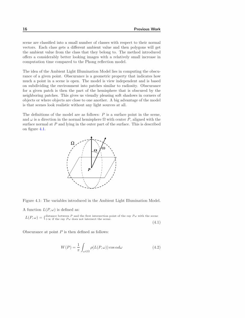
The definitions of the model are as follows: P is a surface point in the scene,and ω is a direction in the normal hemisphere Ω with center P , aligned with thesurface normal at P and lying in the outer part of the surface. This is describedon figure 4.1.
Figure 4.1: The variables introduced in the Ambient Light Illumination Model.
A function L(P, ω) is defined as:
L(P, ω) = distance between P and the first intersection point of the ray Pω with the scene+∞ if the ray Pω does not intersect the scene.
(4.1)
Obscurance at point P is then defined as follows:
W (P ) =1π
∫ω∈Ω
ρ(L(P, ω)) cos αdω (4.2)
4.2 The Model Refined 17
Where:
• ρ(L(P, ω)) is an empirical mapping function that maps the distance L(P, ω)to the first obscuring patch in a given direction to the energy coming fromthis direction to patch P . The function takes values between 0 and 1.
• α is the angle between the direction ω and the normal at point P .
For any surface point P , W (P ) will always take values between 0 and 1. Ob-scurance value 1 means that the patch is fully open, thus it had no intersectionon the visible hemisphere and 0 means fully closed.
4.2 The Model Refined
The Ambient Light Illumination Model has been refined and simplified over theyears by the gaming and movie industries and is now commonly called AmbientOcclusion.
In the ambient light illumination model, obscurance is defined as the percentageof ambient light that should reach each point P . Recent implementations[4,9, 19, 20] reverse the meaning of this and define ambient occlusion to be thepercentage of ambient light that is blocked by the surrounding environment ofpoint P .
Ambient occlusion is then defined as:
A(P ) =1π
∫ω∈Ω
V (P, ω) cos αdω (4.3)
Where V (P, ω) is the visibility function that has value 0 when no geometry isvisible in direction ω and 1 otherwise. Note that this is opposite of the obscu-rance formula. The biggest difference is that the distance mapping function isnot used in particular. We only get the value 0 or 1 from V (P, ω) for any ω.
There is in fact no particular difference between the words obscurance and oc-clusion. Objects can be obscured from light, thus being in shadow. Objects canbe occluded by other objects and then being in shadow. The ambient light illu-mination model only talks about obscurances and never occlusion. Somewherealong the way the word occlusion gained popularity and ambient occlusion be-came well known.
18 Previous Work
There are many recent implementations that use either the ambient light illu-mination model or the simplified ambient occlusion. Many times there are someenhancements introduced, where often the goal is a real-time ambient occlusionsolution.
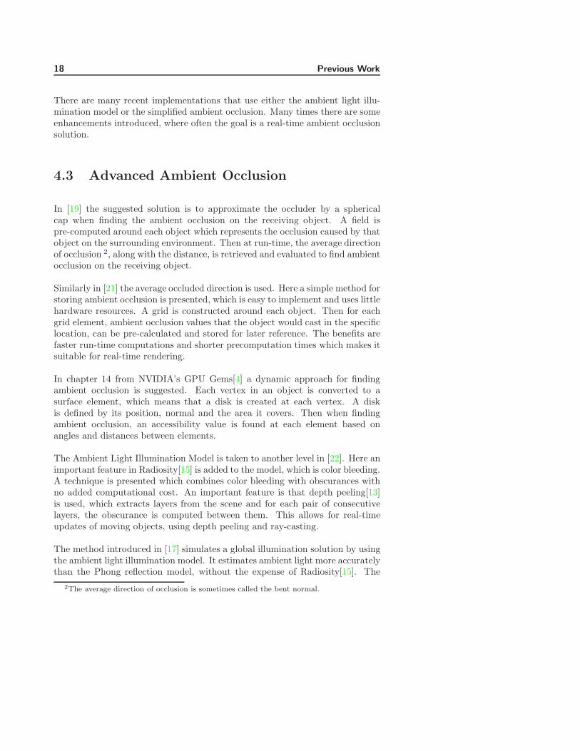
4.3 Advanced Ambient Occlusion
In [19] the suggested solution is to approximate the occluder by a sphericalcap when finding the ambient occlusion on the receiving object. A field ispre-computed around each object which represents the occlusion caused by thatobject on the surrounding environment. Then at run-time, the average directionof occlusion 2, along with the distance, is retrieved and evaluated to find ambientocclusion on the receiving object.
Similarly in [21] the average occluded direction is used. Here a simple method forstoring ambient occlusion is presented, which is easy to implement and uses littlehardware resources. A grid is constructed around each object. Then for eachgrid element, ambient occlusion values that the object would cast in the specificlocation, can be pre-calculated and stored for later reference. The benefits arefaster run-time computations and shorter precomputation times which makes itsuitable for real-time rendering.
In chapter 14 from NVIDIA’s GPU Gems[4] a dynamic approach for findingambient occlusion is suggested. Each vertex in an object is converted to asurface element, which means that a disk is created at each vertex. A diskis defined by its position, normal and the area it covers. Then when findingambient occlusion, an accessibility value is found at each element based onangles and distances between elements.
The Ambient Light Illumination Model is taken to another level in [22]. Here animportant feature in Radiosity[15] is added to the model, which is color bleeding.A technique is presented which combines color bleeding with obscurances withno added computational cost. An important feature is that depth peeling[13]is used, which extracts layers from the scene and for each pair of consecutivelayers, the obscurance is computed between them. This allows for real-timeupdates of moving objects, using depth peeling and ray-casting.
The method introduced in [17] simulates a global illumination solution by usingthe ambient light illumination model. It estimates ambient light more accuratelythan the Phong reflection model, without the expense of Radiosity[15]. The
2The average direction of occlusion is sometimes called the bent normal.
4.3 Advanced Ambient Occlusion 19
illumination computations are stored in obscurance map textures, which areused together with the base textures in the scene. By storing the occlusionvalues in textures, fine shading details and faster rendering can be achieved.This model generates patches, similar to radiosity, by first assigning polygons toclusters according to a certain criteria and then the clusters are subdivided intopatches. Then, similar to methods described earlier, the distance and directionis used to find the incoming ambient light at each point, using the previouslygenerated patches.
Industrial Light and Magic have developed a lighting technique which includeswhat they call Reflection Occlusion and Ambient Environments[20]. Both tech-niques use a ray-traced occlusion pass that is independent of the final lighting.The latter, Ambient Environment, consists of two things which are AmbientEnvironment Lights and Ambient Occlusion. The purpose of ambient environ-ments is to eliminate the need of using a lot of fill lights. Ambient occlusion isan important element in the creation of realistic ambient environment. There isan ambient occlusion pass and the results are baked into an ambient occlusionmap for later reference.

20 Previous Work
Chapter 5
Occlusion Solution
As has been discussed, the goal is to create a natural looking overall illuminationeffect, ambient occlusion to be precise. Following is the flow of how the goal isachieved.
5.1 General Approach
We will calculate ambient occlusion with the use if ray-tracing or specifically,ray casting. This means that for a given point on a surface, rays will be cast inrandom directions relative to that points normal vector. We keep track of howmany rays intersect the scene and find the ratio with the total number of raysthat were shot. This would give us a good approximation of how much eachpoint is obscured from the rest of the scene. This can be seen on figure 3.3 onpage 14. By doing it like this we only need two know two things for any givenpoint of a surface, which is the location of the point and the normal vector ofthe point. Details of how this is implemented is discussed in section 7.4.
22 Occlusion Solution
5.1.1 Alternatives
We could use the extended ambient term[6] for finding ambient values. This isnot an ambient occlusion approach but still a possibility for obtaining decentambient values on an object. When using the extended ambient term, thetriangles in the mesh would be classified into a small number of classes accordingto their normal vectors. Each class will have a different ambient value that isassociated with the triangles in the class. A triangle will then get the ambientvalue that his class has and the result will be a better result than only using oneconstant ambient value for the whole scene like when using the ambient termin the Phong reflection model[23]. This is a simple approach and is just a smallenhancement from the constant ambient value in the Phong model. We wantto get more detailed ambient values.
We have the possibility to go all the way and apply e.g. radiosity[15] to ourobject. Then we would get a very realistic illumination including the ambientocclusion effect. Radiosity is a computationally expensive algorithm and istherefore avoided here. We are aiming at a simple ambient occlusion solutionbut not an overall global illumination that considers light sources and reflections.
We will use the general approach which is ray casting. Now we need to decidehow to apply ray casting on an object for calculating ambient values.
5.2 Using Vertices
We state that we want to find ambient occlusion for a mesh. A mesh is a way todescribe how a model looks like. It contains at least some vertices and normalsalong with information about how the vertices are structured so that they canform the object. Now we need to identify what approach we can use to findthe ambient occlusion that we want. We start by considering using the verticesdirectly, since then we have the values needed, which are the vertex locationsand the normal vector for each vertex. We traverse the vertices in the objectand find how much each vertex is obscured from the rest of the scene. Raysare cast out from each vertex and we find a ratio between how many rays hitthe scene and the total number of rays, which will be our ambient value. Eachambient value is then associated with the corresponding vertex and the objectcan be shaded with ambient occlusion.
By using the vertices we introduce a problem. Imagine a complex object thathas some parts that are highly tesselated for details but also has areas that are
5.2 Using Vertices 23
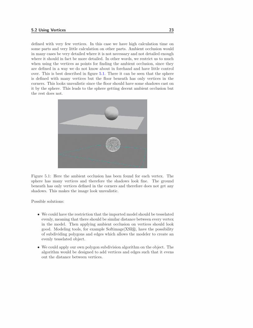
defined with very few vertices. In this case we have high calculation time onsome parts and very little calculation on other parts. Ambient occlusion wouldin many cases be very detailed where it is not necessary and not detailed enoughwhere it should in fact be more detailed. In other words, we restrict us to muchwhen using the vertices as points for finding the ambient occlusion, since theyare defined in a way we do not know about in forehand and have little controlover. This is best described in figure 5.1. There it can be seen that the sphereis defined with many vertices but the floor beneath has only vertices in thecorners. This looks unrealistic since the floor should have some shadows cast onit by the sphere. This leads to the sphere getting decent ambient occlusion butthe rest does not.
Figure 5.1: Here the ambient occlusion has been found for each vertex. Thesphere has many vertices and therefore the shadows look fine. The groundbeneath has only vertices defined in the corners and therefore does not get anyshadows. This makes the image look unrealistic.
Possible solutions:
• We could have the restriction that the imported model should be tesselatedevenly, meaning that there should be similar distance between every vertexin the model. Then applying ambient occlusion on vertices should lookgood. Modeling tools, for example Softimage|XSI, have the possibilityof subdividing polygons and edges which allows the modeler to create anevenly tesselated object.
• We could apply our own polygon subdivision algorithm on the object. Thealgorithm would be designed to add vertices and edges such that it evensout the distance between vertices.
24 Occlusion Solution
• Another possibility is that we apply a texture manually to the model.Then we calculate ambient values for relevant parts of the texture bycasting rays and store the values in the texture for display. This wouldgive us evenly distributed ambient occlusion on an object no matter theunderlying triangle structure.
• It would be possible to create a solid 3D texture to store the ambientvalues. Then for points at the surface of the object, ambient values willbe found and stored in the solid texture and displayed.
• One possibility could be to change the topology of the object by for exam-ple splitting it up in to individual pieces. Then we apply separate textureon each piece that ambient values are found for.
• We could use multiple textures. Then we cluster triangles together andeach cluster will have a local texture mapped to it. This sound similar tosplitting up the object but is in fact a little bit different since here we arenot changing the structure of the model.
It is not desirable to have the restriction that the model should be evenly tesse-lated, since then the model would possibly be defined with more vertices thanwould be needed. The number of vertices greatly affects rendering time and thefewer they are the faster the image will be rendered. Similarly, applying ourown polygon subdivision algorithm will cause the same problem.
Applying a texture manually and finding ambient values for the applied texturewould be a suitable solution. The downside is that we are restricting the modelerto do more work than he would like. It is a good practice not to put to muchrestrictions on the user, but keep implementations as simple and automatic aspossible.
Applying a 3D texture to the entire object is very inefficient and therefore nota desirable option.
Last we have the possibility of applying multiple textures on an object. Oneway would be to split the model into parts and treat each part independentlyand apply a texture on each part. Other way is to keep the object intact butstill have multiple textures that are each applied on different parts of the object.The latter is more appealing since then we keep our model intact.
5.3 Using Textures 25
5.3 Using Textures
We will use multiple local textures which we assign to polygon clusters. We thenneed to cluster the polygons together and apply separate local textures to eachcluster. This leads to us getting continuous texture mapping for each cluster.This approach is similar as before but eliminates using the vertices for findingand storing the ambient occlusion. The idea is based on an idea presented in[17] where the polygons are clustered together. We now find ambient occlusionfor each texel in a texture. A texel is one part of a texture. This will leadto us finding ambient values evenly over the whole object, no matter how theunderlying polygon structure is. Finally we assign texture coordinates to thevertices in the clusters.
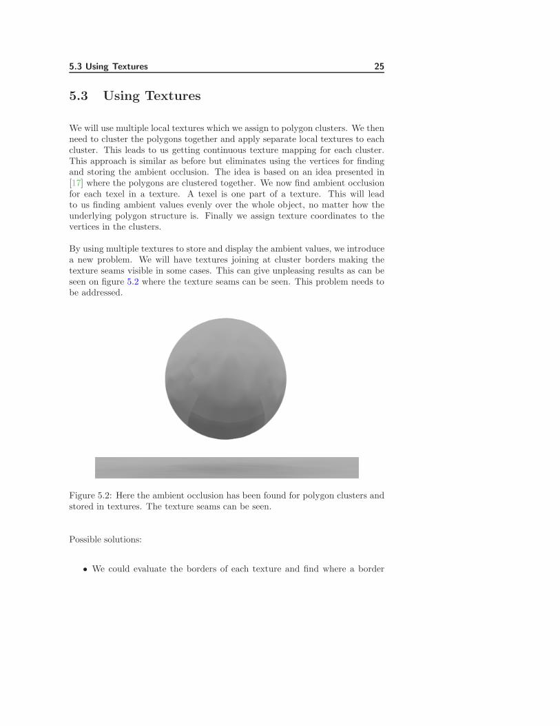
By using multiple textures to store and display the ambient values, we introducea new problem. We will have textures joining at cluster borders making thetexture seams visible in some cases. This can give unpleasing results as can beseen on figure 5.2 where the texture seams can be seen. This problem needs tobe addressed.
Figure 5.2: Here the ambient occlusion has been found for polygon clusters andstored in textures. The texture seams can be seen.
Possible solutions:
• We could evaluate the borders of each texture and find where a border
26 Occlusion Solution
is connected to another texture border. Then we could share the bordersbetween two textures or blend between the ambient values at the bor-ders, where the textures are adjacent to one another. Similar approach issuggested in [17].
• As before we could create a 3D texture. For points at the surface of theobject, ambient values will be found and stored in the solid texture anddisplayed. There should not be any visible seams since we are working onone continuous texture in 3D and therefore the object would get a smoothoverall ambient occlusion.
• Like before we could apply a texture manually on the object and findambient values for it.
• Instead of applying a texture manually we could use another approachwhich is called pelting[5]. Pelting is the process of finding an optimaltexture mapping over a subdivision surface[7]. The result from pelting isa continuous texture over most of the object but there will still be placeswhere a cut is made where seams can be seen.
• We could let the textures overlap. Then we are finding ambient valuesmore than once on some parts of an object which would lead to us wantingto blend between the values.
The problem with sharing or blending between texture borders is that we stillhave multiple textures that are adjacent to one another. Since the textures arenot continuous, and hardware is designed to work in continues texture space,the seams could still be visible.
As before we conclude that using 3D textures is inefficient and do not considerthat anymore.
By applying texture manually we still have the problem of visible texture seams.On many objects, we can’t create a texture where all points have unique texturecoordinates and then we can’t have continuous texture over the whole object.This results in us getting places where there will be visible seams. For examplethere is no way to assign continuous texture coordinates on a sphere so thatevery point is assigned a unique pair of texture coordinates.
If we would use pelting we will almost have a continuous texture space overthe whole object. A temporary cut is made in the object and there textureseams can be visible when the texture is applied. In [5], a scheme is introducedthat blends smoothly over the cut, between different texture mappings on thesubdivision surface. The final result is a seamless texture on an object.
5.4 Blending Textures 27
The pelting approach would therefore solve our problem of having visible textureseams. The idea of making multiple textures overlap and blend between themwould also work and since we already have multiple textures we will continuein that direction. Therefore our solution would be to introduce the overlappingof textures that then needs to be blended.
5.4 Blending Textures
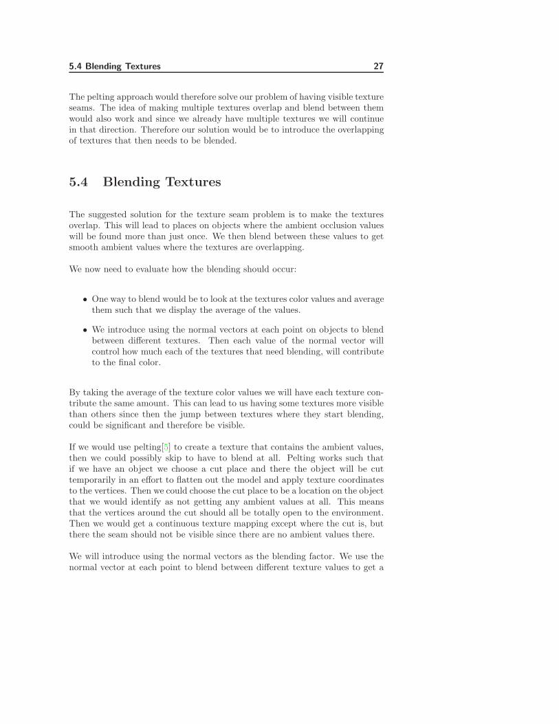
The suggested solution for the texture seam problem is to make the texturesoverlap. This will lead to places on objects where the ambient occlusion valueswill be found more than just once. We then blend between these values to getsmooth ambient values where the textures are overlapping.
We now need to evaluate how the blending should occur:
• One way to blend would be to look at the textures color values and averagethem such that we display the average of the values.
• We introduce using the normal vectors at each point on objects to blendbetween different textures. Then each value of the normal vector willcontrol how much each of the textures that need blending, will contributeto the final color.
By taking the average of the texture color values we will have each texture con-tribute the same amount. This can lead to us having some textures more visiblethan others since then the jump between textures where they start blending,could be significant and therefore be visible.
If we would use pelting[5] to create a texture that contains the ambient values,then we could possibly skip to have to blend at all. Pelting works such thatif we have an object we choose a cut place and there the object will be cuttemporarily in an effort to flatten out the model and apply texture coordinatesto the vertices. Then we could choose the cut place to be a location on the objectthat we would identify as not getting any ambient values at all. This meansthat the vertices around the cut should all be totally open to the environment.Then we would get a continuous texture mapping except where the cut is, butthere the seam should not be visible since there are no ambient values there.
We will introduce using the normal vectors as the blending factor. We use thenormal vector at each point to blend between different texture values to get a
28 Occlusion Solution
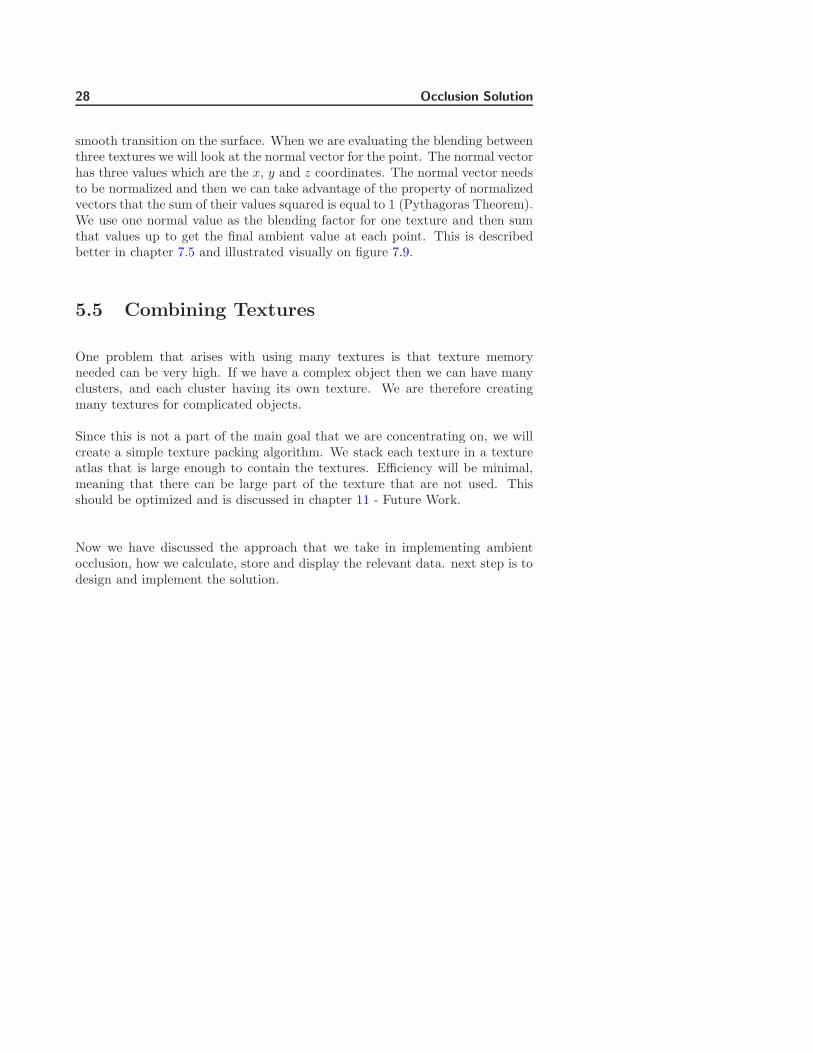
smooth transition on the surface. When we are evaluating the blending betweenthree textures we will look at the normal vector for the point. The normal vectorhas three values which are the x, y and z coordinates. The normal vector needsto be normalized and then we can take advantage of the property of normalizedvectors that the sum of their values squared is equal to 1 (Pythagoras Theorem).We use one normal value as the blending factor for one texture and then sumthat values up to get the final ambient value at each point. This is describedbetter in chapter 7.5 and illustrated visually on figure 7.9.
5.5 Combining Textures
One problem that arises with using many textures is that texture memoryneeded can be very high. If we have a complex object then we can have manyclusters, and each cluster having its own texture. We are therefore creatingmany textures for complicated objects.
Since this is not a part of the main goal that we are concentrating on, we willcreate a simple texture packing algorithm. We stack each texture in a textureatlas that is large enough to contain the textures. Efficiency will be minimal,meaning that there can be large part of the texture that are not used. Thisshould be optimized and is discussed in chapter 11 - Future Work.
Now we have discussed the approach that we take in implementing ambientocclusion, how we calculate, store and display the relevant data. next step is todesign and implement the solution.

Chapter 6
Design
6.1 Import/Export
There are many ways for exchanging digital assets. Usually developers have theirown format which means that exchanging the assets can be difficult when theyneed to be used by other applications than from the developer that created it.COLLADA[3] is an effort to eliminate this problem, by providing a schema thatallows applications to freely exchange digital assets without loss of information.COLLADA stands for COLLAborative Design Activity. Here we will discussthe available data representation in COLLADA along with what we choose forthis implementation. More details about COLLADA and some history can befound in appendix A.
The geometry data is imported from a COLLADA file. The name of the file isdefined at runtime and the scene can then be imported and used in the ambientocclusion calculations. When the calculations are done, the new data will beexported in a new COLLADA file that the user has defined at runtime.
30 Design
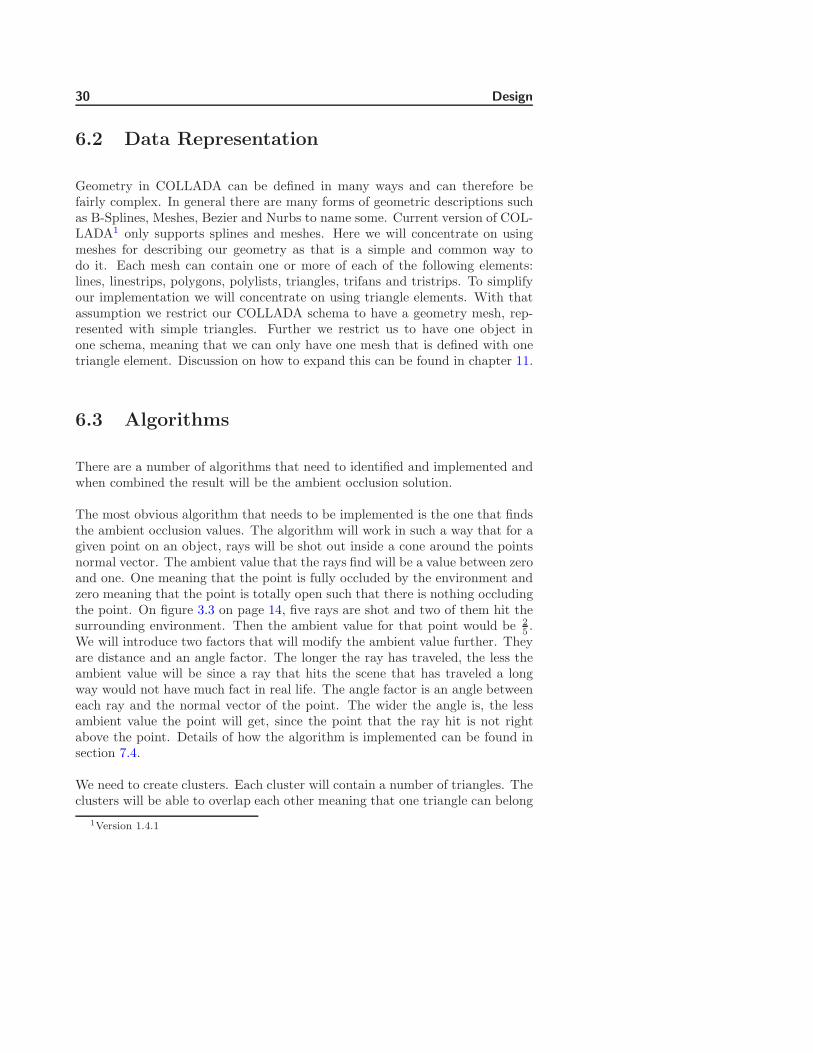
6.2 Data Representation
Geometry in COLLADA can be defined in many ways and can therefore befairly complex. In general there are many forms of geometric descriptions suchas B-Splines, Meshes, Bezier and Nurbs to name some. Current version of COL-LADA1 only supports splines and meshes. Here we will concentrate on usingmeshes for describing our geometry as that is a simple and common way todo it. Each mesh can contain one or more of each of the following elements:lines, linestrips, polygons, polylists, triangles, trifans and tristrips. To simplifyour implementation we will concentrate on using triangle elements. With thatassumption we restrict our COLLADA schema to have a geometry mesh, rep-resented with simple triangles. Further we restrict us to have one object inone schema, meaning that we can only have one mesh that is defined with onetriangle element. Discussion on how to expand this can be found in chapter 11.
6.3 Algorithms
There are a number of algorithms that need to identified and implemented andwhen combined the result will be the ambient occlusion solution.
The most obvious algorithm that needs to be implemented is the one that findsthe ambient occlusion values. The algorithm will work in such a way that for agiven point on an object, rays will be shot out inside a cone around the pointsnormal vector. The ambient value that the rays find will be a value between zeroand one. One meaning that the point is fully occluded by the environment andzero meaning that the point is totally open such that there is nothing occludingthe point. On figure 3.3 on page 14, five rays are shot and two of them hit thesurrounding environment. Then the ambient value for that point would be 2
5 .We will introduce two factors that will modify the ambient value further. Theyare distance and an angle factor. The longer the ray has traveled, the less theambient value will be since a ray that hits the scene that has traveled a longway would not have much fact in real life. The angle factor is an angle betweeneach ray and the normal vector of the point. The wider the angle is, the lessambient value the point will get, since the point that the ray hit is not rightabove the point. Details of how the algorithm is implemented can be found insection 7.4.
We need to create clusters. Each cluster will contain a number of triangles. Theclusters will be able to overlap each other meaning that one triangle can belong
1Version 1.4.1
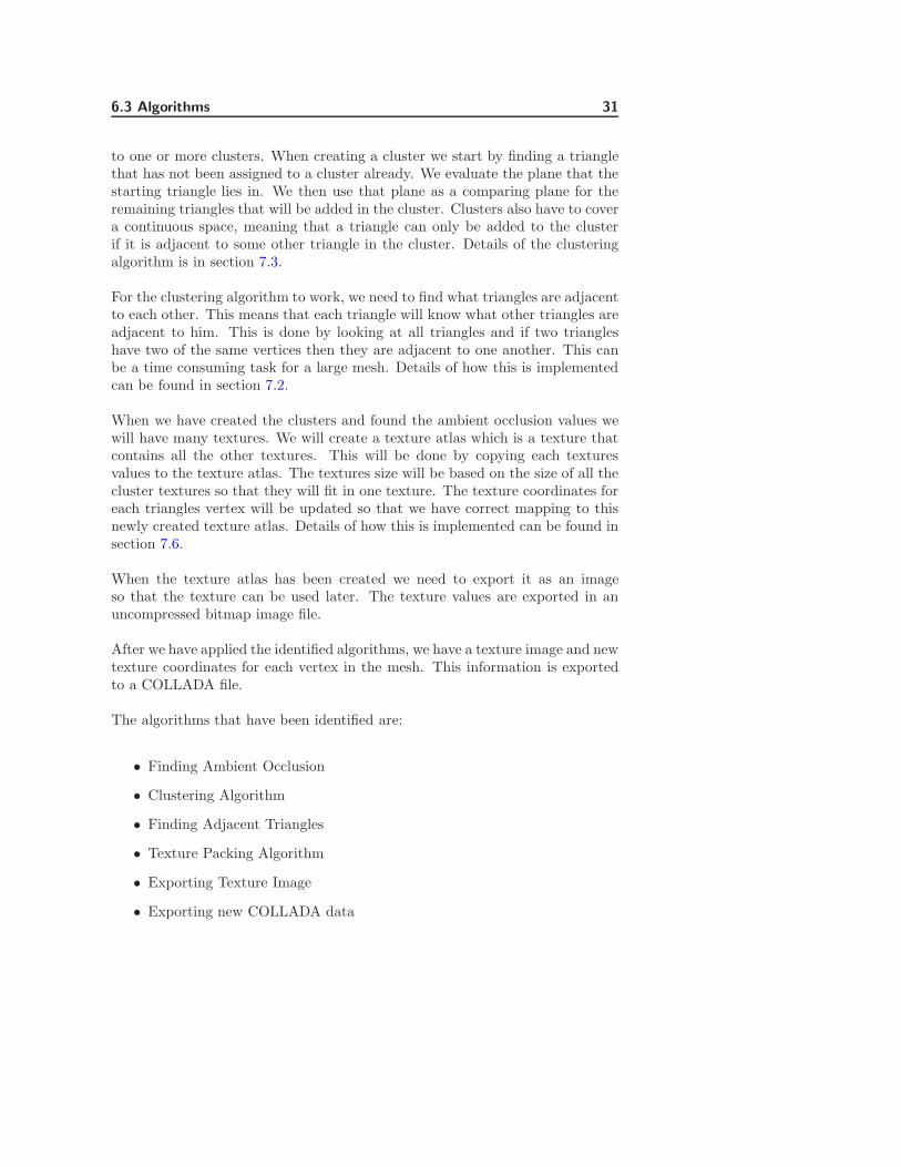
6.3 Algorithms 31
to one or more clusters. When creating a cluster we start by finding a trianglethat has not been assigned to a cluster already. We evaluate the plane that thestarting triangle lies in. We then use that plane as a comparing plane for theremaining triangles that will be added in the cluster. Clusters also have to covera continuous space, meaning that a triangle can only be added to the clusterif it is adjacent to some other triangle in the cluster. Details of the clusteringalgorithm is in section 7.3.
For the clustering algorithm to work, we need to find what triangles are adjacentto each other. This means that each triangle will know what other triangles areadjacent to him. This is done by looking at all triangles and if two triangleshave two of the same vertices then they are adjacent to one another. This canbe a time consuming task for a large mesh. Details of how this is implementedcan be found in section 7.2.
When we have created the clusters and found the ambient occlusion values wewill have many textures. We will create a texture atlas which is a texture thatcontains all the other textures. This will be done by copying each texturesvalues to the texture atlas. The textures size will be based on the size of all thecluster textures so that they will fit in one texture. The texture coordinates foreach triangles vertex will be updated so that we have correct mapping to thisnewly created texture atlas. Details of how this is implemented can be found insection 7.6.
When the texture atlas has been created we need to export it as an imageso that the texture can be used later. The texture values are exported in anuncompressed bitmap image file.
After we have applied the identified algorithms, we have a texture image and newtexture coordinates for each vertex in the mesh. This information is exportedto a COLLADA file.
The algorithms that have been identified are:
• Finding Ambient Occlusion
• Clustering Algorithm
• Finding Adjacent Triangles
• Texture Packing Algorithm
• Exporting Texture Image
• Exporting new COLLADA data
32 Design
6.4 Objects
The design is object oriented. Therefore the objects needed for the implemen-tation need to be identified.
First we will need triangle objects that store the data that defines one trianglein three dimensions. A triangle will contain three vertices and normal vectorsfor each vertex. That information is enough to define a triangle but we needsomething more. It is possible to obtain the center of the triangle which isfound using the vertices. Since a triangle always lies in a plane, we will be ableto access the normal vector of the triangles plane. Each triangle will have aunique integer ID and it will also contain the IDs of the cluster that it belongsto. Each vertex in a triangle can have three texture coordinates associated withthem. Triangles need to know which triangles are adjacent to them and thereforethey will have a list of adjacent triangles. Finally there are two variables thatare used when triangle clusters are created. These are a variable indicating ifthe triangle has been assigned to a cluster or not, and a value indicating thestate of the triangle.
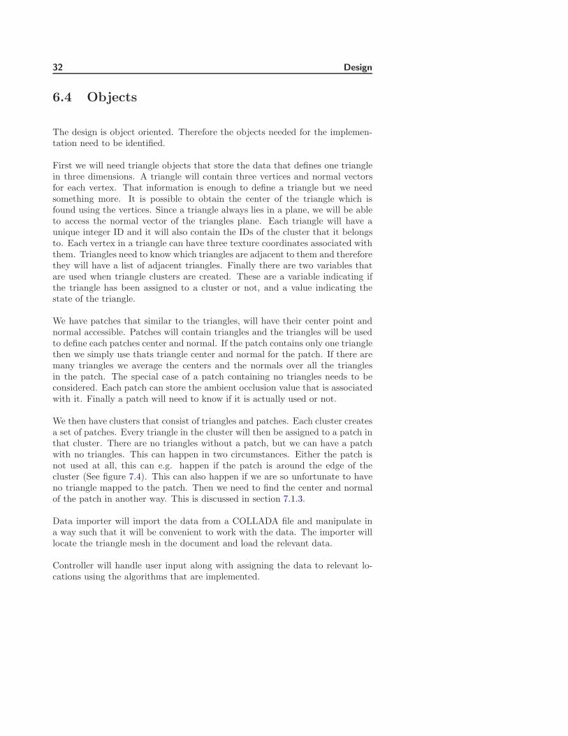
We have patches that similar to the triangles, will have their center point andnormal accessible. Patches will contain triangles and the triangles will be usedto define each patches center and normal. If the patch contains only one trianglethen we simply use thats triangle center and normal for the patch. If there aremany triangles we average the centers and the normals over all the trianglesin the patch. The special case of a patch containing no triangles needs to beconsidered. Each patch can store the ambient occlusion value that is associatedwith it. Finally a patch will need to know if it is actually used or not.
We then have clusters that consist of triangles and patches. Each cluster createsa set of patches. Every triangle in the cluster will then be assigned to a patch inthat cluster. There are no triangles without a patch, but we can have a patchwith no triangles. This can happen in two circumstances. Either the patch isnot used at all, this can e.g. happen if the patch is around the edge of thecluster (See figure 7.4). This can also happen if we are so unfortunate to haveno triangle mapped to the patch. Then we need to find the center and normalof the patch in another way. This is discussed in section 7.1.3.
Data importer will import the data from a COLLADA file and manipulate ina way such that it will be convenient to work with the data. The importer willlocate the triangle mesh in the document and load the relevant data.
Controller will handle user input along with assigning the data to relevant lo-cations using the algorithms that are implemented.
6.5 Final Structure 33
The objects that have been identified and will be implemented are:
• Triangles
• Patches
• Clusters
• Data Container
• Controller
6.5 Final Structure
The structure and relations between objects can bee seen in the UML diagramon figure 6.1.
The algorithms mentioned earlier will all be located in the myMain class exceptthe ambient occlusion algorithm, which will be located in a myCluster object.
myMain is the controller. He starts by instantiating a myDAEdata object withthe COLLADA file as input. myDAEdata loads the data into a database withuse of a helper class called myMesh. What myMesh does is that he loads aCOLLADA mesh element and extracts information from it that can then beretrieved from myMesh. The information needed from the COLLADA input fileare the vertices, normals and faces of the triangle mesh. After the file has beenloaded and the relevant data extracted from it the controller will start creatingmyTriangle objects and from the triangles he creates myCluster objects. Theneach cluster will create a number of myPatch objects. Now all the objects havebeen created. Implementation details about the objects are discussed in chapter7.
There are two other helper classes in the diagram which are myRandomRaysand myQueue. The first class will create a certain number of random rays thatare used for finding ambient occlusion. The queue class is used by the controllerwhen the clusters are created. The random ray generator is discussed in section7.4.1 and the queue class in section 7.3.1.

34 Design
Figure 6.1: UML Diagram showing the objects in the solution and the relation-ship between them.
Chapter 7
Implementation
We need to implement the objects and algorithm that have been identified inthe design chapter. First we discuss the flow of the data relative to the objects.Then we go into details about each object that is implemented. Following thatis a dedicated section for each of the algorithms that have been identified.
7.1 Data Structure
We have interactions and connections between objects which can be seen on theUML diagram presented in section 6.5. The basic flow of the program relativeto the data is as follows. After importing a model we use it to create triangleobjects. The model has to be defined with simple triangles. Softimage|XSIwas used when creating models for rendering and testing. Softimage has thepossibility of exporting scenes in a COLLADA document and it offers the possi-bility of converting all polygons to triangles. Softimage is discussed in appendixA. Each of the imported triangles will be associated with one or more clusters.Each cluster will then contain a set of triangles along with a set of patches. Eachpatch will be assigned a number of triangles belonging to that cluster, so thateach patch will have zero or more triangles. Then ambient occlusion values arefound for each patch in a cluster and the values stored as textures. After this is
36 Implementation
done we create one texture from the cluster textures, export the texture imageand write the new COLLADA data back to a file. We will now discuss eachobject that makes up our data structure, the important variables and methods.
7.1.1 Triangle
A triangle can be thought of as the most primitive object in the data structure.Each triangle has a unique integer ID. To define a triangle we need to set itsthree vertices and the normal vector for each vertex.
When the vertices have been set we find the center of the triangle by averagingover the three vertices. Similarly the triangles planes normal vector is found byusing the vertices.
Each triangle will belong to one, two or three clusters. It should not happenthat triangle is assigned to more than three clusters. This could happen if thecomparing angle when creating clusters is to low. Each triangle has a unique IDand all the IDs of the clusters that the triangle belongs to can be accessed toknow what clusters it belongs to. Also the number of clusters that one trianglebelongs to can be accessed.
Each triangles vertex will have texture coordinates assigned to it. One vertexwill always have three texture coordinates assigned to it, irrelevant of how manyclusters it belongs to. The reason for this is to simplify the implementation. Thisallows us to add three texture coordinates to each vertex and create a texturethat contains all the ambient values. In most cases a triangle will belong to onecluster. So that when a texture coordinate is added for the first time to trianglesvertices, we add those coordinates to all three texture coordinates. This will leadto us blending between the same values of a texture if the triangle only belongsto one cluster in the end. When and if the second and third texture coordinatesare added, we add that coordinate to the relevant texture coordinate variablesin the triangle. The three texture coordinates are stored in three variables thatcan be accessed globally.
There are two variables that belongs to triangles that are used when we arecreating clusters from the triangles. One is a boolean variable indicating if thetriangle has been assigned to a cluster or not. The other is an integer variablethat can have three states that are used in the Breath-first search algorithm. Thestates are white, gray or black and are defined as integer values. All trianglesstart with the default value of white, meaning that the triangle has not beenevaluated in the search algorithm. Then when the algorithm is working the statecan go to grey and black. This is discussed in detail in section 7.3.1. There are
7.1 Data Structure 37
two other variables that are a part of the search algorithm that are not usedhere but still implemented. They are the ID of the predecessor of each triangleand the distance in the search three that this triangle has with the triangle webegan with.
Each triangle needs to know what other triangles are lying adjacent to him.Therefore each triangle contains a list of IDs of the triangles that are adjacentto him. This adjacency list is created by the algorithm described in section 7.2.The adjacency list is then used in the clustering algorithm described in section7.3
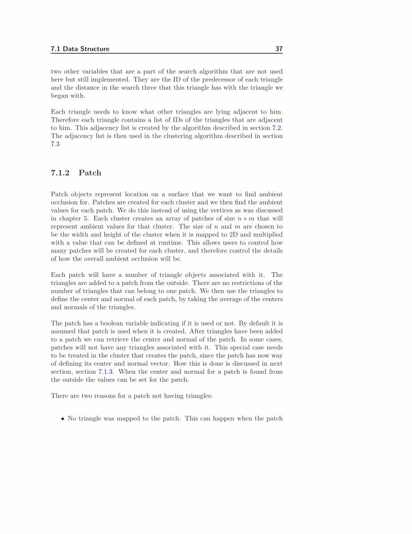
7.1.2 Patch
Patch objects represent location on a surface that we want to find ambientocclusion for. Patches are created for each cluster and we then find the ambientvalues for each patch. We do this instead of using the vertices as was discussedin chapter 5. Each cluster creates an array of patches of size n ∗ m that willrepresent ambient values for that cluster. The size of n and m are chosen tobe the width and height of the cluster when it is mapped to 2D and multipliedwith a value that can be defined at runtime. This allows users to control howmany patches will be created for each cluster, and therefore control the detailsof how the overall ambient occlusion will be.
Each patch will have a number of triangle objects associated with it. Thetriangles are added to a patch from the outside. There are no restrictions of thenumber of triangles that can belong to one patch. We then use the triangles todefine the center and normal of each patch, by taking the average of the centersand normals of the triangles.
The patch has a boolean variable indicating if it is used or not. By default it isassumed that patch is used when it is created. After triangles have been addedto a patch we can retrieve the center and normal of the patch. In some cases,patches will not have any triangles associated with it. This special case needsto be treated in the cluster that creates the patch, since the patch has now wayof defining its center and normal vector. How this is done is discussed in nextsection, section 7.1.3. When the center and normal for a patch is found fromthe outside the values can be set for the patch.
There are two reasons for a patch not having triangles:
• No triangle was mapped to the patch. This can happen when the patch
38 Implementation
resolution is set higher than the number of triangles in the cluster.
• The patch is not used at all. This can happen in many cases since a clusteris usually not exactly formed as a n ∗ m square (See figure 7.4).
In the first case we find the center and normal of the patch in another way, sincethe patch is used but has no triangles. In the latter case the patch is not usedand we set a variable in the patch indicating that the patch is not used.
Finally each patch will store the ambient occlusion value that is associated withit.
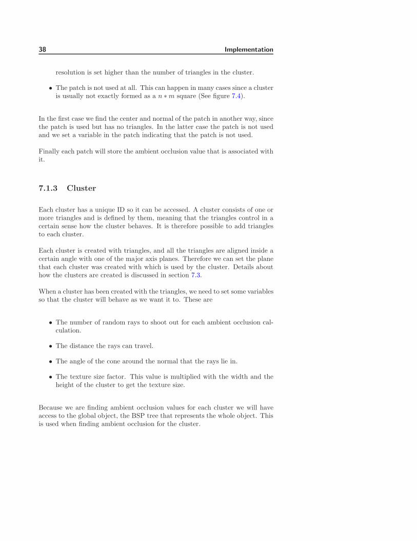
7.1.3 Cluster
Each cluster has a unique ID so it can be accessed. A cluster consists of one ormore triangles and is defined by them, meaning that the triangles control in acertain sense how the cluster behaves. It is therefore possible to add trianglesto each cluster.
Each cluster is created with triangles, and all the triangles are aligned inside acertain angle with one of the major axis planes. Therefore we can set the planethat each cluster was created with which is used by the cluster. Details abouthow the clusters are created is discussed in section 7.3.
When a cluster has been created with the triangles, we need to set some variablesso that the cluster will behave as we want it to. These are
• The number of random rays to shoot out for each ambient occlusion cal-culation.
• The distance the rays can travel.
• The angle of the cone around the normal that the rays lie in.
• The texture size factor. This value is multiplied with the width and theheight of the cluster to get the texture size.
Because we are finding ambient occlusion values for each cluster we will haveaccess to the global object, the BSP tree that represents the whole object. Thisis used when finding ambient occlusion for the cluster.
7.1 Data Structure 39
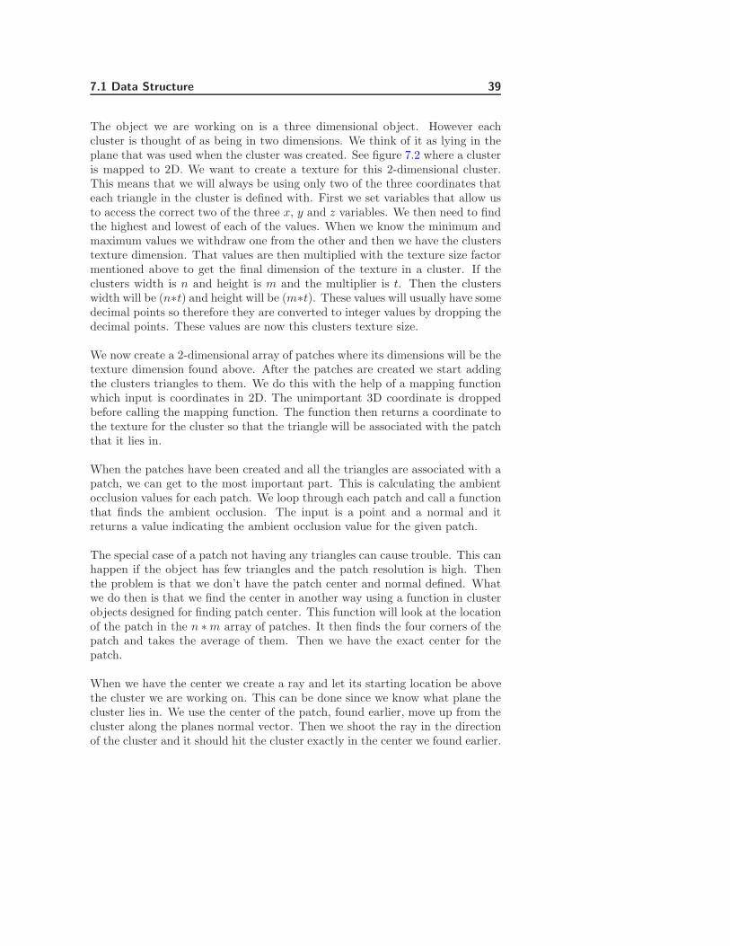
The object we are working on is a three dimensional object. However eachcluster is thought of as being in two dimensions. We think of it as lying in theplane that was used when the cluster was created. See figure 7.2 where a clusteris mapped to 2D. We want to create a texture for this 2-dimensional cluster.This means that we will always be using only two of the three coordinates thateach triangle in the cluster is defined with. First we set variables that allow usto access the correct two of the three x, y and z variables. We then need to findthe highest and lowest of each of the values. When we know the minimum andmaximum values we withdraw one from the other and then we have the clusterstexture dimension. That values are then multiplied with the texture size factormentioned above to get the final dimension of the texture in a cluster. If theclusters width is n and height is m and the multiplier is t. Then the clusterswidth will be (n∗t) and height will be (m∗t). These values will usually have somedecimal points so therefore they are converted to integer values by dropping thedecimal points. These values are now this clusters texture size.
We now create a 2-dimensional array of patches where its dimensions will be thetexture dimension found above. After the patches are created we start addingthe clusters triangles to them. We do this with the help of a mapping functionwhich input is coordinates in 2D. The unimportant 3D coordinate is droppedbefore calling the mapping function. The function then returns a coordinate tothe texture for the cluster so that the triangle will be associated with the patchthat it lies in.
When the patches have been created and all the triangles are associated with apatch, we can get to the most important part. This is calculating the ambientocclusion values for each patch. We loop through each patch and call a functionthat finds the ambient occlusion. The input is a point and a normal and itreturns a value indicating the ambient occlusion value for the given patch.
The special case of a patch not having any triangles can cause trouble. This canhappen if the object has few triangles and the patch resolution is high. Thenthe problem is that we don’t have the patch center and normal defined. Whatwe do then is that we find the center in another way using a function in clusterobjects designed for finding patch center. This function will look at the locationof the patch in the n ∗ m array of patches. It then finds the four corners of thepatch and takes the average of them. Then we have the exact center for thepatch.
When we have the center we create a ray and let its starting location be abovethe cluster we are working on. This can be done since we know what plane thecluster lies in. We use the center of the patch, found earlier, move up from thecluster along the planes normal vector. Then we shoot the ray in the directionof the cluster and it should hit the cluster exactly in the center we found earlier.
40 Implementation
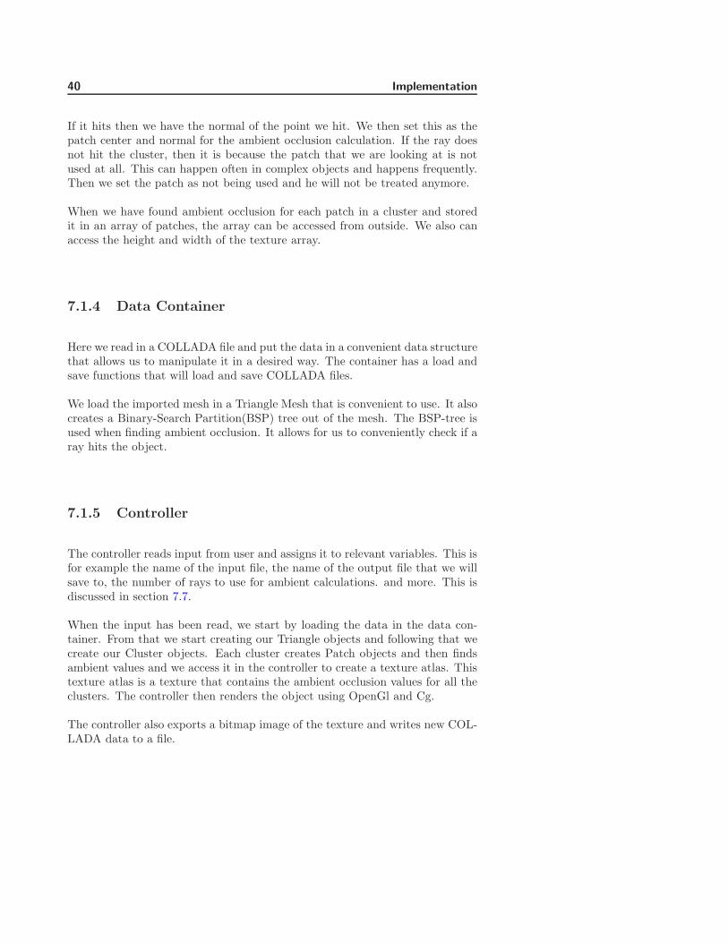
If it hits then we have the normal of the point we hit. We then set this as thepatch center and normal for the ambient occlusion calculation. If the ray doesnot hit the cluster, then it is because the patch that we are looking at is notused at all. This can happen often in complex objects and happens frequently.Then we set the patch as not being used and he will not be treated anymore.
When we have found ambient occlusion for each patch in a cluster and storedit in an array of patches, the array can be accessed from outside. We also canaccess the height and width of the texture array.
7.1.4 Data Container
Here we read in a COLLADA file and put the data in a convenient data structurethat allows us to manipulate it in a desired way. The container has a load andsave functions that will load and save COLLADA files.
We load the imported mesh in a Triangle Mesh that is convenient to use. It alsocreates a Binary-Search Partition(BSP) tree out of the mesh. The BSP-tree isused when finding ambient occlusion. It allows for us to conveniently check if aray hits the object.
7.1.5 Controller
The controller reads input from user and assigns it to relevant variables. This isfor example the name of the input file, the name of the output file that we willsave to, the number of rays to use for ambient calculations. and more. This isdiscussed in section 7.7.
When the input has been read, we start by loading the data in the data con-tainer. From that we start creating our Triangle objects and following that wecreate our Cluster objects. Each cluster creates Patch objects and then findsambient values and we access it in the controller to create a texture atlas. Thistexture atlas is a texture that contains the ambient occlusion values for all theclusters. The controller then renders the object using OpenGl and Cg.
The controller also exports a bitmap image of the texture and writes new COL-LADA data to a file.
7.2 Finding Adjacent Triangles 41
7.2 Finding Adjacent Triangles
Each triangle needs to know which other triangles are adjacent to him, whichis used when creating triangle clusters. This simple algorithm will loop throughall triangles and compare it to all the other triangles. If they share two verticesthen we have two adjacent triangles and they can be added on each othersadjacent triangles list. Actually though this algorithm is simple to implementit can be very time consuming. If we have N triangles, then for each vertex wewould look at N − 1 triangles, which makes it an algorithm of type O(n2).
The calculation is lowered slightly by using the fact that when working withtriangles, each triangle will have at most three adjacent triangles, and exactlythree when working on a closed mesh. This fact allows us to stop looking attriangles when we have already found all the triangles adjacent to the one weare looking at at each time. With this the calculation time is lowered slightly,since we only consider triangles that we have not found three adjacent trianglesfor.
7.3 Clustering Algorithm
Each cluster will be assigned a unique ID which will go from 0 to n − 1 wheren is the number of clusters found. The clustering algorithm loops through alltriangles and registers if they have been processed or not. When all trianglesare processed the algorithm can successfully quit. We now have signed all thetriangles to one or more clusters. The clustering algorithm uses an abbreviationof the Breadth-first search(BFS) algorithm found in the book Introduction toAlgorithms[11]. The attributes needed when applying it is that each trianglehas an attribute called color which can have the values white, grey or black.The algorithm is discussed later in the section.
The approach for creating clusters is that we start with a triangle that has notbeen assigned to a cluster. We evaluate the triangle in such a way that wecompare the normal of the triangle, with the normal of one of the major axisplanes. The major axis planes are three, the XY -plane, the XZ-plane and theY Z-plane. We find what plane, our starting triangle is closest to by comparingthe triangles normal with the axis planes normal. The axis plane that has thesmallest angle will be used as comparison for the rest of the triangles that wewant to put in the current cluster.
When assigning a triangle to a cluster we do it only if the following criteria is
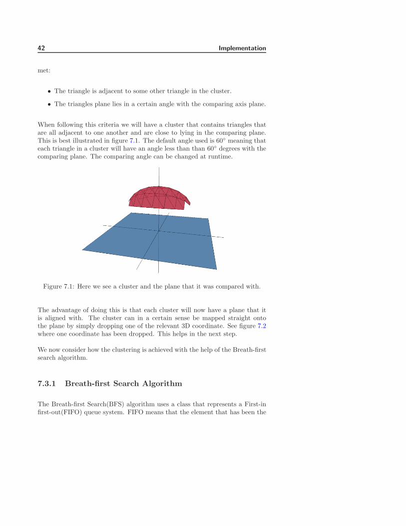
42 Implementation
met:
• The triangle is adjacent to some other triangle in the cluster.
• The triangles plane lies in a certain angle with the comparing axis plane.
When following this criteria we will have a cluster that contains triangles thatare all adjacent to one another and are close to lying in the comparing plane.This is best illustrated in figure 7.1. The default angle used is 60 meaning thateach triangle in a cluster will have an angle less than than 60 degrees with thecomparing plane. The comparing angle can be changed at runtime.
Figure 7.1: Here we see a cluster and the plane that it was compared with.
The advantage of doing this is that each cluster will now have a plane that itis aligned with. The cluster can in a certain sense be mapped straight ontothe plane by simply dropping one of the relevant 3D coordinate. See figure 7.2where one coordinate has been dropped. This helps in the next step.
We now consider how the clustering is achieved with the help of the Breath-firstsearch algorithm.
7.3.1 Breath-first Search Algorithm
The Breath-first Search(BFS) algorithm uses a class that represents a First-infirst-out(FIFO) queue system. FIFO means that the element that has been the
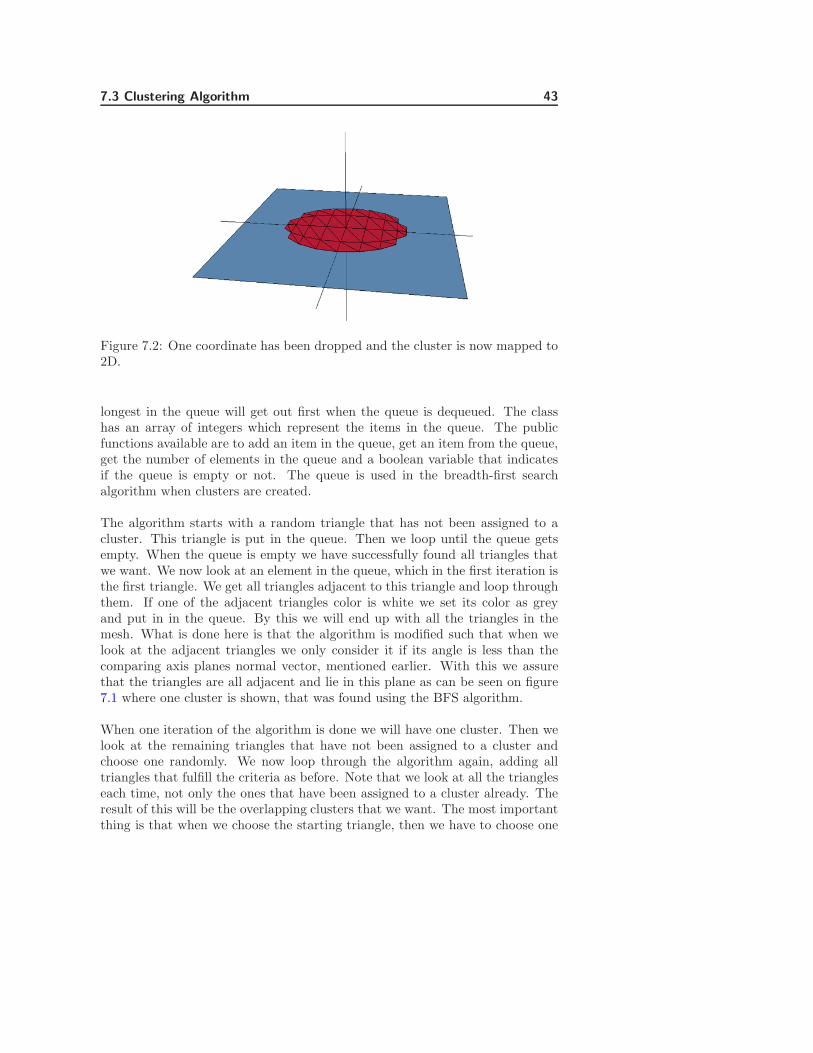
7.3 Clustering Algorithm 43
Figure 7.2: One coordinate has been dropped and the cluster is now mapped to2D.
longest in the queue will get out first when the queue is dequeued. The classhas an array of integers which represent the items in the queue. The publicfunctions available are to add an item in the queue, get an item from the queue,get the number of elements in the queue and a boolean variable that indicatesif the queue is empty or not. The queue is used in the breadth-first searchalgorithm when clusters are created.
The algorithm starts with a random triangle that has not been assigned to acluster. This triangle is put in the queue. Then we loop until the queue getsempty. When the queue is empty we have successfully found all triangles thatwe want. We now look at an element in the queue, which in the first iteration isthe first triangle. We get all triangles adjacent to this triangle and loop throughthem. If one of the adjacent triangles color is white we set its color as greyand put in in the queue. By this we will end up with all the triangles in themesh. What is done here is that the algorithm is modified such that when welook at the adjacent triangles we only consider it if its angle is less than thecomparing axis planes normal vector, mentioned earlier. With this we assurethat the triangles are all adjacent and lie in this plane as can be seen on figure7.1 where one cluster is shown, that was found using the BFS algorithm.
When one iteration of the algorithm is done we will have one cluster. Then welook at the remaining triangles that have not been assigned to a cluster andchoose one randomly. We now loop through the algorithm again, adding alltriangles that fulfill the criteria as before. Note that we look at all the triangleseach time, not only the ones that have been assigned to a cluster already. Theresult of this will be the overlapping clusters that we want. The most importantthing is that when we choose the starting triangle, then we have to choose one
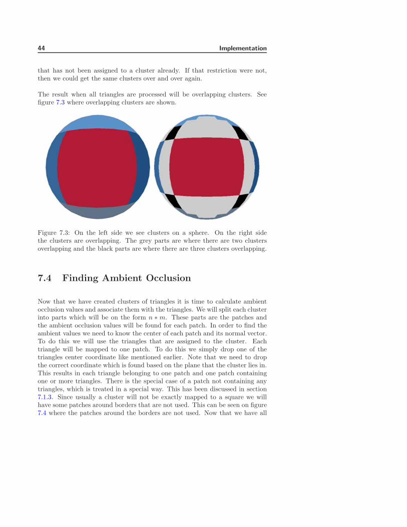
44 Implementation
that has not been assigned to a cluster already. If that restriction were not,then we could get the same clusters over and over again.
The result when all triangles are processed will be overlapping clusters. Seefigure 7.3 where overlapping clusters are shown.
Figure 7.3: On the left side we see clusters on a sphere. On the right sidethe clusters are overlapping. The grey parts are where there are two clustersoverlapping and the black parts are where there are three clusters overlapping.
7.4 Finding Ambient Occlusion
Now that we have created clusters of triangles it is time to calculate ambientocclusion values and associate them with the triangles. We will split each clusterinto parts which will be on the form n ∗ m. These parts are the patches andthe ambient occlusion values will be found for each patch. In order to find theambient values we need to know the center of each patch and its normal vector.To do this we will use the triangles that are assigned to the cluster. Eachtriangle will be mapped to one patch. To do this we simply drop one of thetriangles center coordinate like mentioned earlier. Note that we need to dropthe correct coordinate which is found based on the plane that the cluster lies in.This results in each triangle belonging to one patch and one patch containingone or more triangles. There is the special case of a patch not containing anytriangles, which is treated in a special way. This has been discussed in section7.1.3. Since usually a cluster will not be exactly mapped to a square we willhave some patches around borders that are not used. This can be seen on figure7.4 where the patches around the borders are not used. Now that we have all
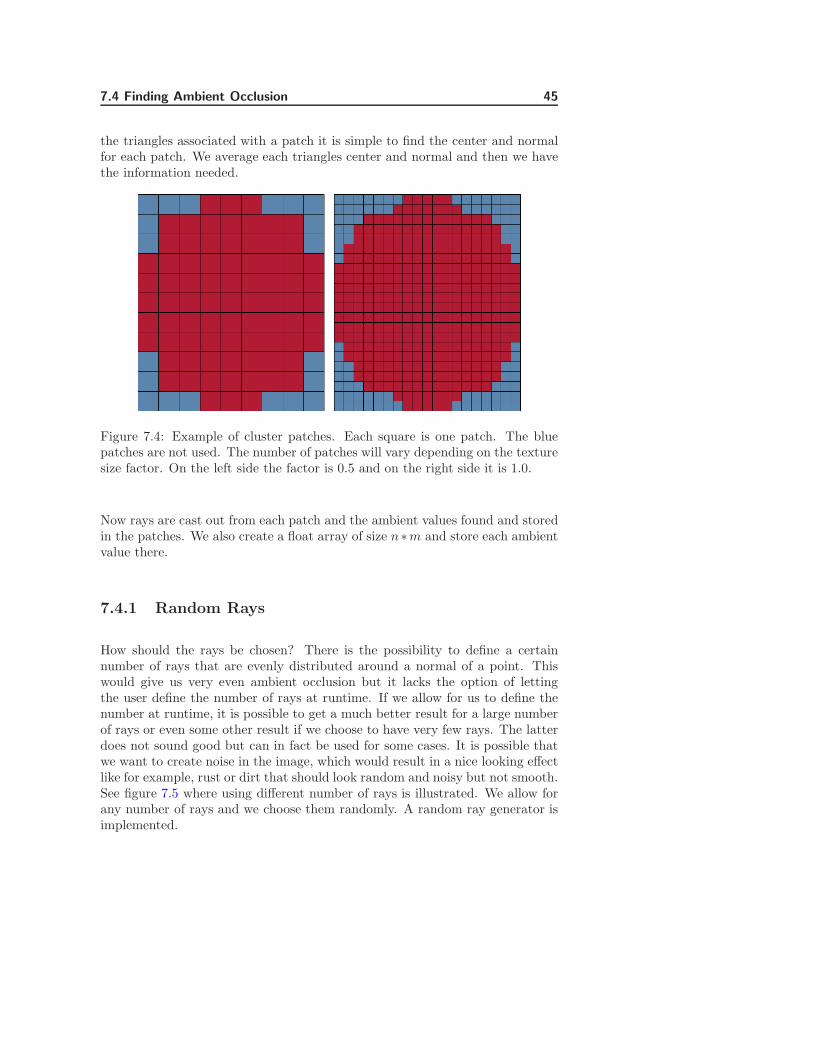
7.4 Finding Ambient Occlusion 45
the triangles associated with a patch it is simple to find the center and normalfor each patch. We average each triangles center and normal and then we havethe information needed.
Figure 7.4: Example of cluster patches. Each square is one patch. The bluepatches are not used. The number of patches will vary depending on the texturesize factor. On the left side the factor is 0.5 and on the right side it is 1.0.
Now rays are cast out from each patch and the ambient values found and storedin the patches. We also create a float array of size n∗m and store each ambientvalue there.
7.4.1 Random Rays
How should the rays be chosen? There is the possibility to define a certainnumber of rays that are evenly distributed around a normal of a point. Thiswould give us very even ambient occlusion but it lacks the option of lettingthe user define the number of rays at runtime. If we allow for us to define thenumber at runtime, it is possible to get a much better result for a large numberof rays or even some other result if we choose to have very few rays. The latterdoes not sound good but can in fact be used for some cases. It is possible thatwe want to create noise in the image, which would result in a nice looking effectlike for example, rust or dirt that should look random and noisy but not smooth.See figure 7.5 where using different number of rays is illustrated. We allow forany number of rays and we choose them randomly. A random ray generator isimplemented.
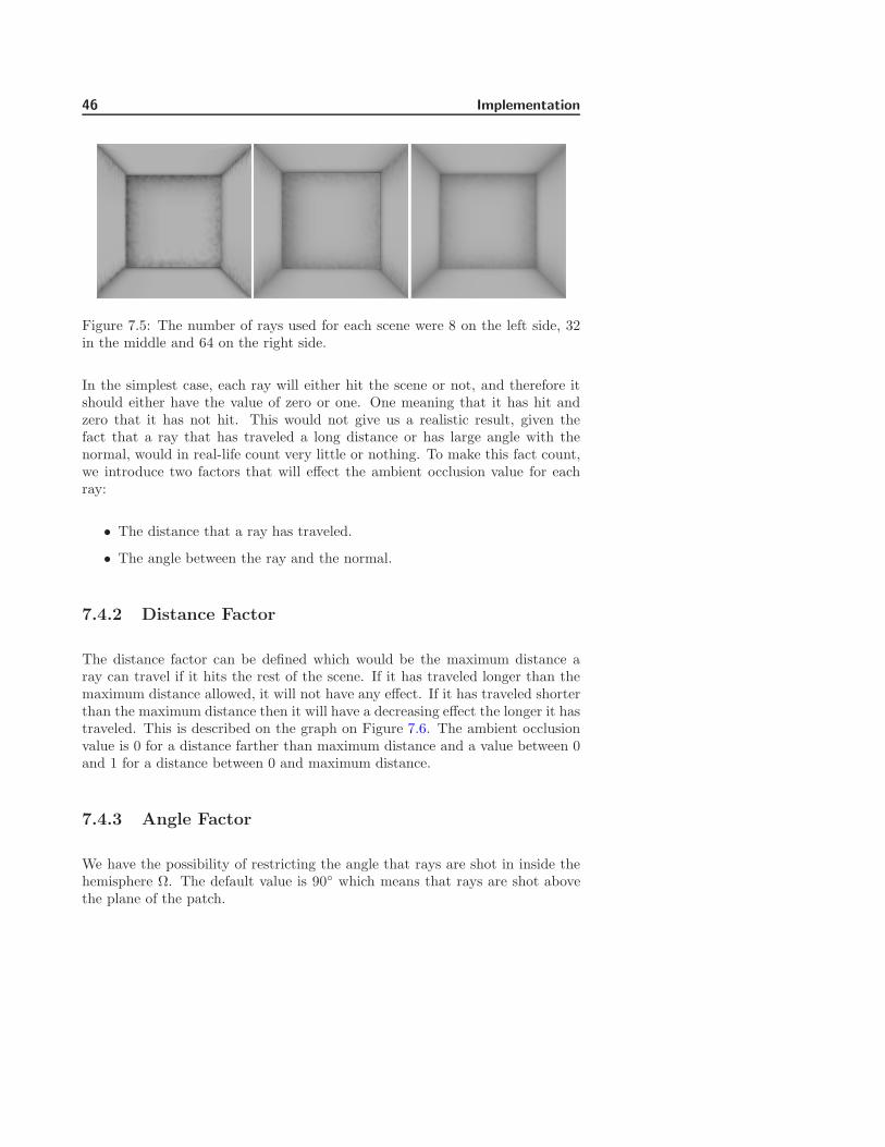
46 Implementation
Figure 7.5: The number of rays used for each scene were 8 on the left side, 32in the middle and 64 on the right side.
In the simplest case, each ray will either hit the scene or not, and therefore itshould either have the value of zero or one. One meaning that it has hit andzero that it has not hit. This would not give us a realistic result, given thefact that a ray that has traveled a long distance or has large angle with thenormal, would in real-life count very little or nothing. To make this fact count,we introduce two factors that will effect the ambient occlusion value for eachray:
• The distance that a ray has traveled.
• The angle between the ray and the normal.
7.4.2 Distance Factor
The distance factor can be defined which would be the maximum distance aray can travel if it hits the rest of the scene. If it has traveled longer than themaximum distance allowed, it will not have any effect. If it has traveled shorterthan the maximum distance then it will have a decreasing effect the longer it hastraveled. This is described on the graph on Figure 7.6. The ambient occlusionvalue is 0 for a distance farther than maximum distance and a value between 0and 1 for a distance between 0 and maximum distance.
7.4.3 Angle Factor
We have the possibility of restricting the angle that rays are shot in inside thehemisphere Ω. The default value is 90 which means that rays are shot abovethe plane of the patch.
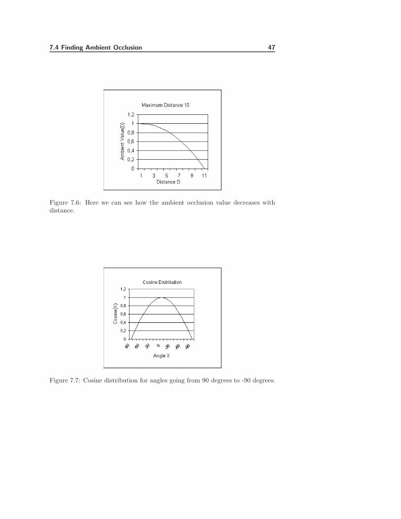
7.4 Finding Ambient Occlusion 47
Figure 7.6: Here we can see how the ambient occlusion value decreases withdistance.
Figure 7.7: Cosine distribution for angles going from 90 degrees to -90 degrees.
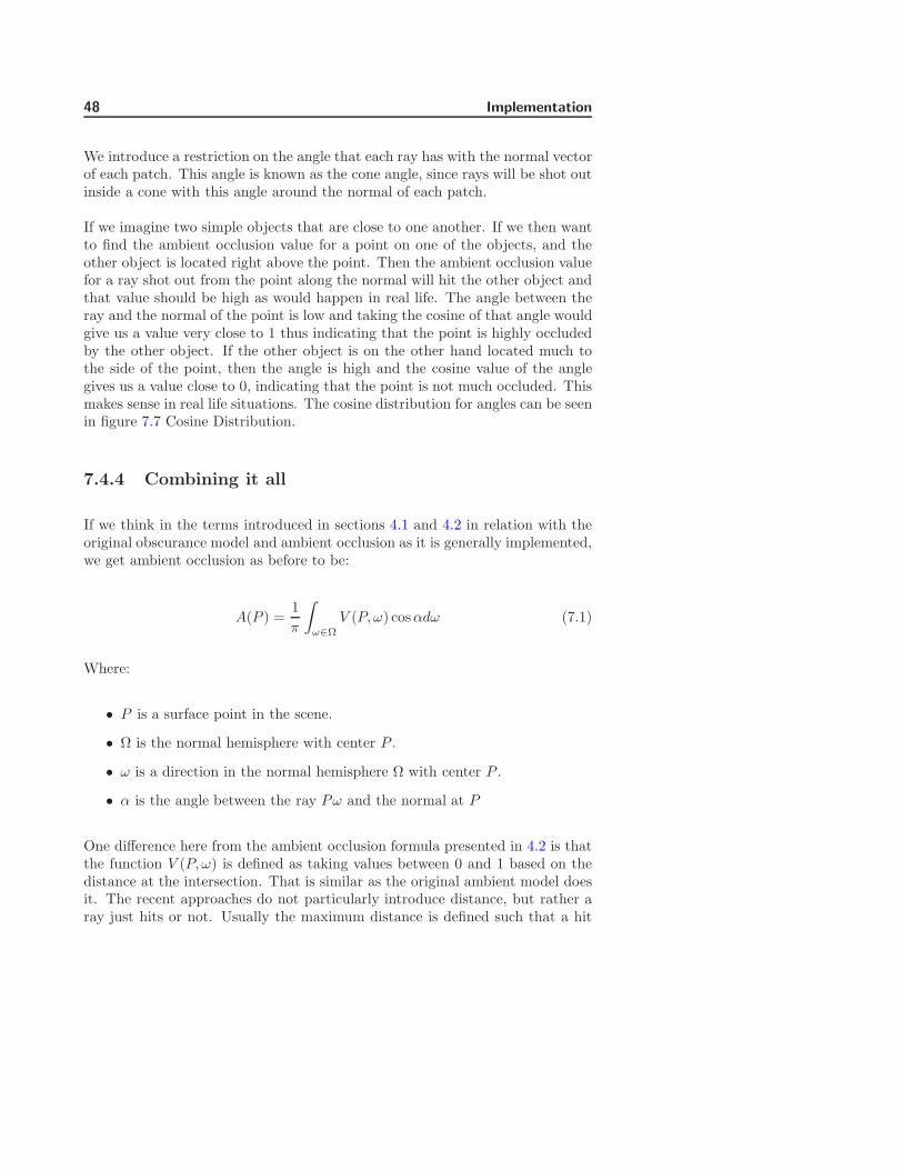
48 Implementation
We introduce a restriction on the angle that each ray has with the normal vectorof each patch. This angle is known as the cone angle, since rays will be shot outinside a cone with this angle around the normal of each patch.
If we imagine two simple objects that are close to one another. If we then wantto find the ambient occlusion value for a point on one of the objects, and theother object is located right above the point. Then the ambient occlusion valuefor a ray shot out from the point along the normal will hit the other object andthat value should be high as would happen in real life. The angle between theray and the normal of the point is low and taking the cosine of that angle wouldgive us a value very close to 1 thus indicating that the point is highly occludedby the other object. If the other object is on the other hand located much tothe side of the point, then the angle is high and the cosine value of the anglegives us a value close to 0, indicating that the point is not much occluded. Thismakes sense in real life situations. The cosine distribution for angles can be seenin figure 7.7 Cosine Distribution.
7.4.4 Combining it all
If we think in the terms introduced in sections 4.1 and 4.2 in relation with theoriginal obscurance model and ambient occlusion as it is generally implemented,we get ambient occlusion as before to be:
A(P ) =1π
∫ω∈Ω
V (P, ω) cosαdω (7.1)
Where:
• P is a surface point in the scene.
• Ω is the normal hemisphere with center P .
• ω is a direction in the normal hemisphere Ω with center P .
• α is the angle between the ray Pω and the normal at P
One difference here from the ambient occlusion formula presented in 4.2 is thatthe function V (P, ω) is defined as taking values between 0 and 1 based on thedistance at the intersection. That is similar as the original ambient model doesit. The recent approaches do not particularly introduce distance, but rather aray just hits or not. Usually the maximum distance is defined such that a hit
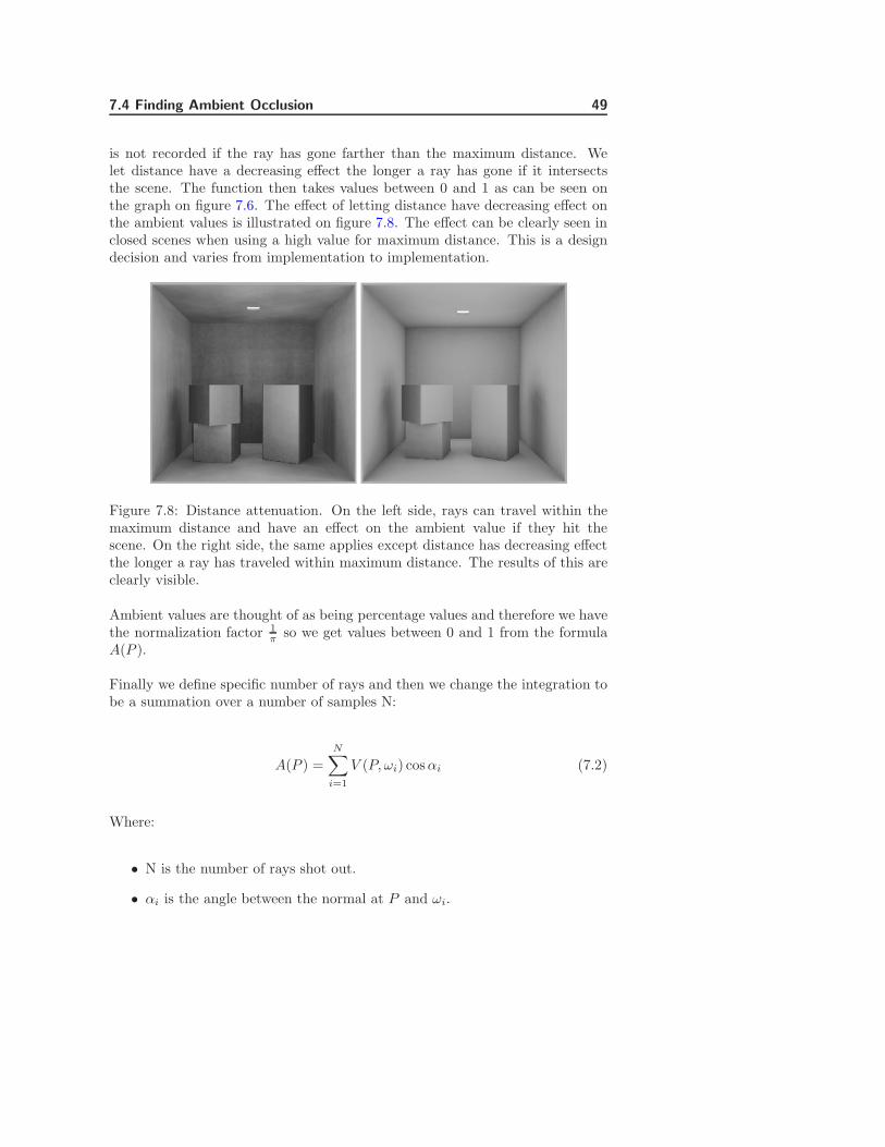
7.4 Finding Ambient Occlusion 49
is not recorded if the ray has gone farther than the maximum distance. Welet distance have a decreasing effect the longer a ray has gone if it intersectsthe scene. The function then takes values between 0 and 1 as can be seen onthe graph on figure 7.6. The effect of letting distance have decreasing effect onthe ambient values is illustrated on figure 7.8. The effect can be clearly seen inclosed scenes when using a high value for maximum distance. This is a designdecision and varies from implementation to implementation.
Figure 7.8: Distance attenuation. On the left side, rays can travel within themaximum distance and have an effect on the ambient value if they hit thescene. On the right side, the same applies except distance has decreasing effectthe longer a ray has traveled within maximum distance. The results of this areclearly visible.
Ambient values are thought of as being percentage values and therefore we havethe normalization factor 1
π so we get values between 0 and 1 from the formulaA(P ).
Finally we define specific number of rays and then we change the integration tobe a summation over a number of samples N:
A(P ) =N∑
i=1
V (P, ωi) cosαi (7.2)
Where:
• N is the number of rays shot out.
• αi is the angle between the normal at P and ωi.
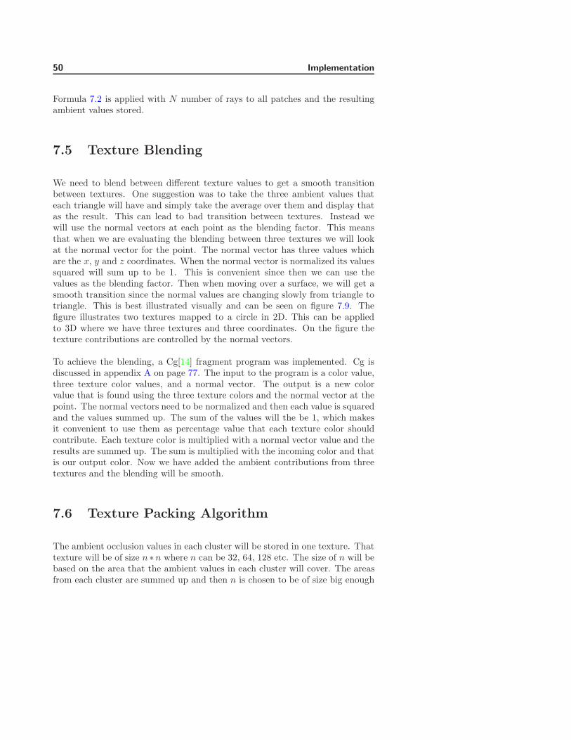
50 Implementation
Formula 7.2 is applied with N number of rays to all patches and the resultingambient values stored.
7.5 Texture Blending
We need to blend between different texture values to get a smooth transitionbetween textures. One suggestion was to take the three ambient values thateach triangle will have and simply take the average over them and display thatas the result. This can lead to bad transition between textures. Instead wewill use the normal vectors at each point as the blending factor. This meansthat when we are evaluating the blending between three textures we will lookat the normal vector for the point. The normal vector has three values whichare the x, y and z coordinates. When the normal vector is normalized its valuessquared will sum up to be 1. This is convenient since then we can use thevalues as the blending factor. Then when moving over a surface, we will get asmooth transition since the normal values are changing slowly from triangle totriangle. This is best illustrated visually and can be seen on figure 7.9. Thefigure illustrates two textures mapped to a circle in 2D. This can be appliedto 3D where we have three textures and three coordinates. On the figure thetexture contributions are controlled by the normal vectors.
To achieve the blending, a Cg[14] fragment program was implemented. Cg isdiscussed in appendix A on page 77. The input to the program is a color value,three texture color values, and a normal vector. The output is a new colorvalue that is found using the three texture colors and the normal vector at thepoint. The normal vectors need to be normalized and then each value is squaredand the values summed up. The sum of the values will the be 1, which makesit convenient to use them as percentage value that each texture color shouldcontribute. Each texture color is multiplied with a normal vector value and theresults are summed up. The sum is multiplied with the incoming color and thatis our output color. Now we have added the ambient contributions from threetextures and the blending will be smooth.
7.6 Texture Packing Algorithm
The ambient occlusion values in each cluster will be stored in one texture. Thattexture will be of size n ∗n where n can be 32, 64, 128 etc. The size of n will bebased on the area that the ambient values in each cluster will cover. The areasfrom each cluster are summed up and then n is chosen to be of size big enough
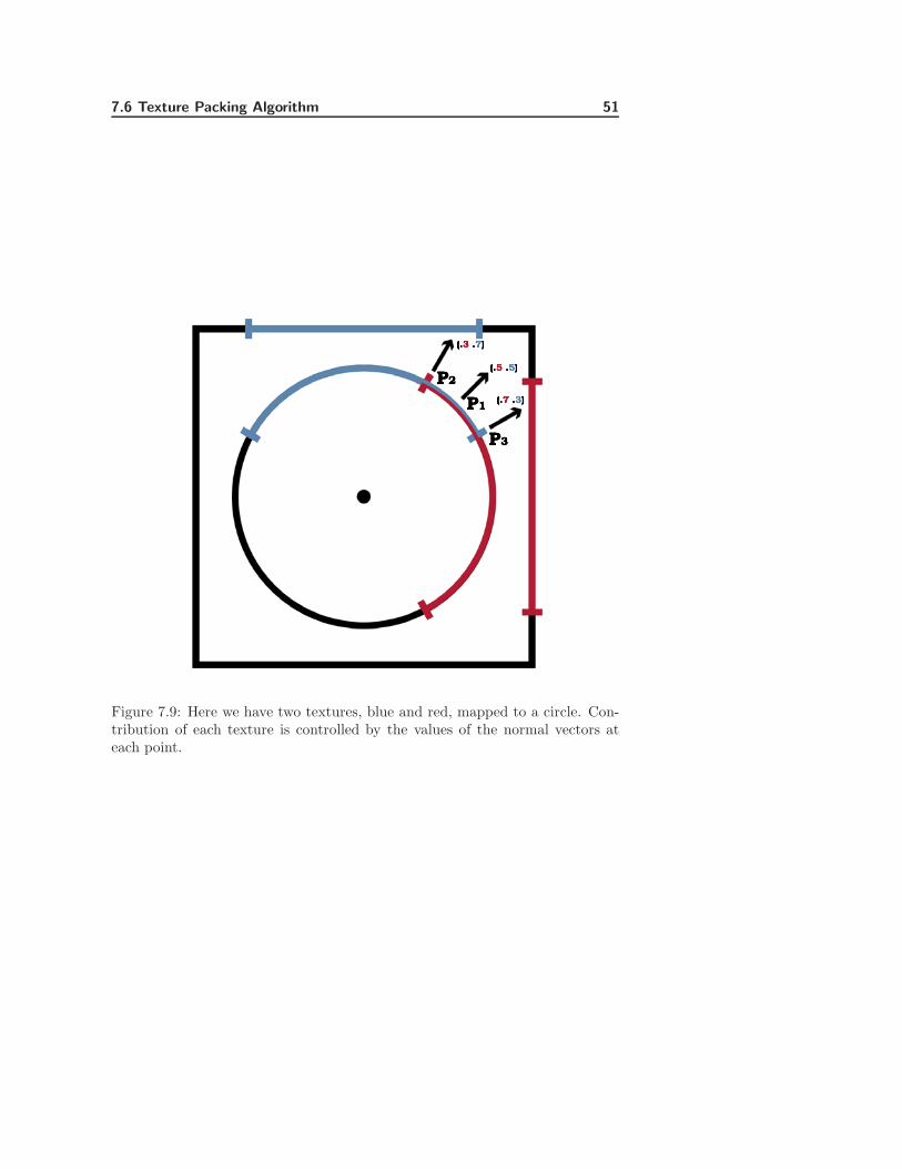
7.6 Texture Packing Algorithm 51
Figure 7.9: Here we have two textures, blue and red, mapped to a circle. Con-tribution of each texture is controlled by the values of the normal vectors ateach point.
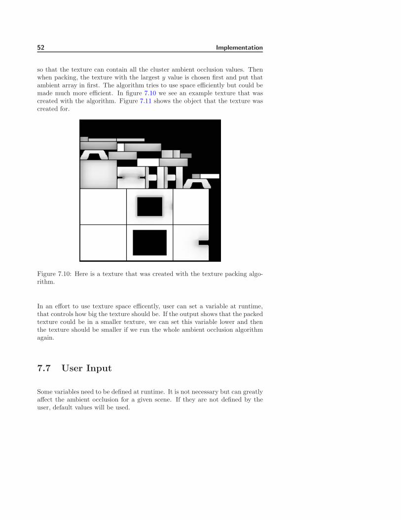
52 Implementation
so that the texture can contain all the cluster ambient occlusion values. Thenwhen packing, the texture with the largest y value is chosen first and put thatambient array in first. The algorithm tries to use space efficiently but could bemade much more efficient. In figure 7.10 we see an example texture that wascreated with the algorithm. Figure 7.11 shows the object that the texture wascreated for.
Figure 7.10: Here is a texture that was created with the texture packing algo-rithm.
In an effort to use texture space efficently, user can set a variable at runtime,that controls how big the texture should be. If the output shows that the packedtexture could be in a smaller texture, we can set this variable lower and thenthe texture should be smaller if we run the whole ambient occlusion algorithmagain.
7.7 User Input
Some variables need to be defined at runtime. It is not necessary but can greatlyaffect the ambient occlusion for a given scene. If they are not defined by theuser, default values will be used.
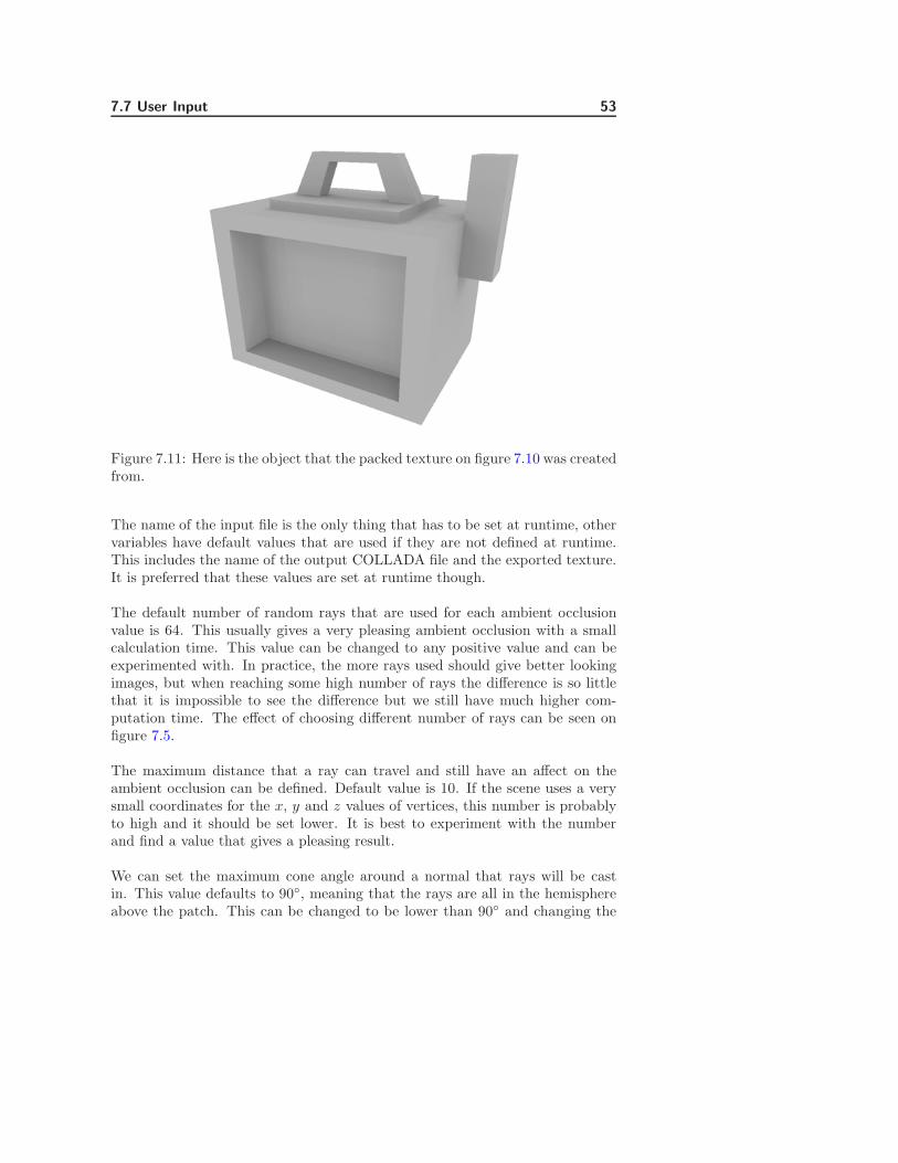
7.7 User Input 53
Figure 7.11: Here is the object that the packed texture on figure 7.10 was createdfrom.
The name of the input file is the only thing that has to be set at runtime, othervariables have default values that are used if they are not defined at runtime.This includes the name of the output COLLADA file and the exported texture.It is preferred that these values are set at runtime though.
The default number of random rays that are used for each ambient occlusionvalue is 64. This usually gives a very pleasing ambient occlusion with a smallcalculation time. This value can be changed to any positive value and can beexperimented with. In practice, the more rays used should give better lookingimages, but when reaching some high number of rays the difference is so littlethat it is impossible to see the difference but we still have much higher com-putation time. The effect of choosing different number of rays can be seen onfigure 7.5.
The maximum distance that a ray can travel and still have an affect on theambient occlusion can be defined. Default value is 10. If the scene uses a verysmall coordinates for the x, y and z values of vertices, this number is probablyto high and it should be set lower. It is best to experiment with the numberand find a value that gives a pleasing result.
We can set the maximum cone angle around a normal that rays will be castin. This value defaults to 90, meaning that the rays are all in the hemisphereabove the patch. This can be changed to be lower than 90 and changing the
54 Implementation
value can give results that are desired for a given scene.
The size of the textures that each cluster will create can be set at runtime. Thetexture size will be a factor of the width and height of each cluster multipliedwith this value. The default value is 3. This can be set much higher if we havea small object that is highly tesselated. This variable can greatly affect theoutcome of the ambient occlusion in a scene.
The default compare angle that is used when clusters are created is 60. Thisvalue can be changed to any value between 50 and 70 degrees. It is sometimesnecessary to change the default value as we can create clusters that are notcorrect. This problem is discussed in chapters 8 and 11.
Chapter 8
Testing
Different scenes were created that tried to catch the aspect of the ambientocclusion program created here. Four scenes were rendered that tried to coverthe things that an implementation like this should be able to handle.
• Scene 1 is a simple Cornell box. The purpose of the scene is to test theoverall visual effect of our ambient occlusion implementation using a scenethat is well known. Number of triangles is 84.
• Scene 2 is a sphere hovering over a plane. The purpose of this scene isto test the effect of using different parameters. We change the number ofrays, the cone angle and the distance. Number of triangles is 3.902.
• Scene 3 is an object that tries to catch the effect of overlapping texturesand the blending between them. It has curved surfaces and thereforeoverlapping of textures. Number of triangles is 34.548.
• Scene 4 is a Utah teapot. Number of triangles is 24.138.
If we talk generally about the scenes. Scene 1 is very simple and therefore haslow calculation time since it only has 84 triangles. The scene catches the overalleffect of the ambient occlusion solution. Figure 8.1 is a rendered image of thescene.
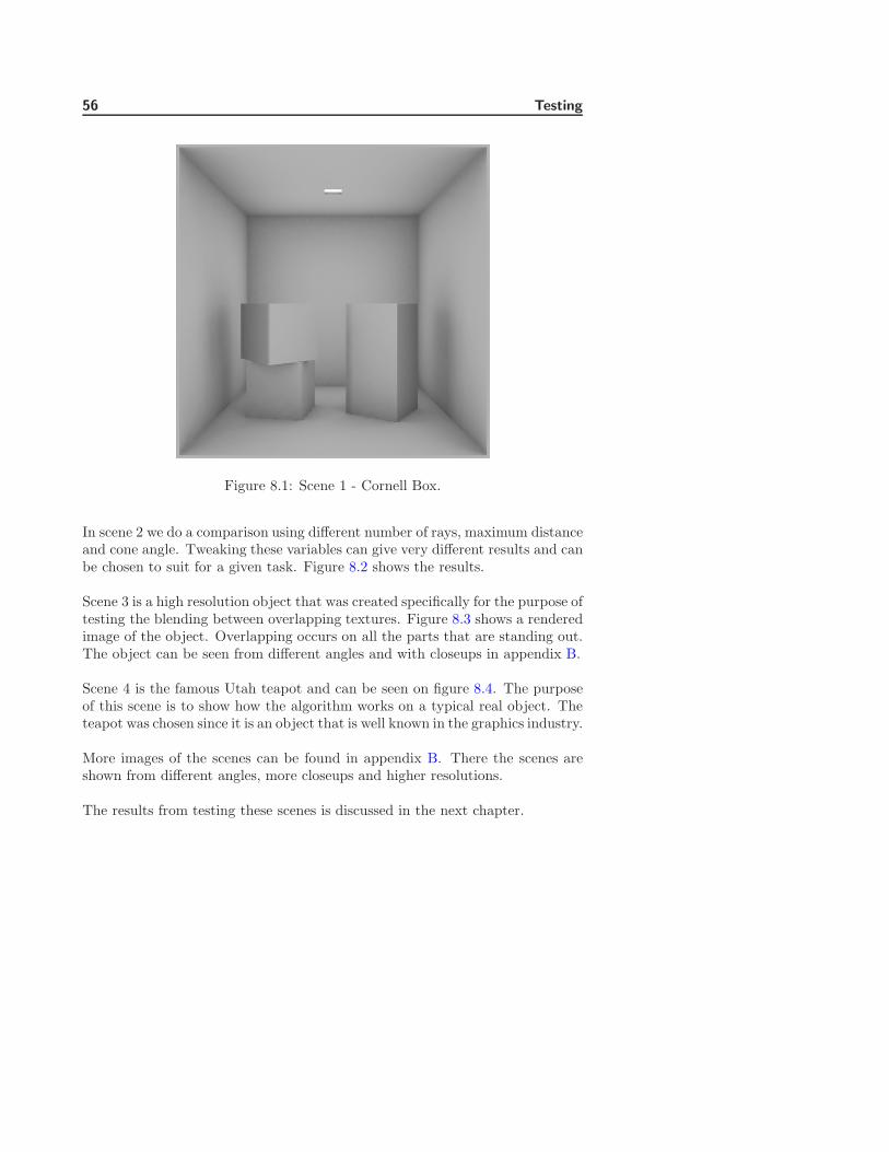
56 Testing
Figure 8.1: Scene 1 - Cornell Box.
In scene 2 we do a comparison using different number of rays, maximum distanceand cone angle. Tweaking these variables can give very different results and canbe chosen to suit for a given task. Figure 8.2 shows the results.
Scene 3 is a high resolution object that was created specifically for the purpose oftesting the blending between overlapping textures. Figure 8.3 shows a renderedimage of the object. Overlapping occurs on all the parts that are standing out.The object can be seen from different angles and with closeups in appendix B.
Scene 4 is the famous Utah teapot and can be seen on figure 8.4. The purposeof this scene is to show how the algorithm works on a typical real object. Theteapot was chosen since it is an object that is well known in the graphics industry.
More images of the scenes can be found in appendix B. There the scenes areshown from different angles, more closeups and higher resolutions.
The results from testing these scenes is discussed in the next chapter.
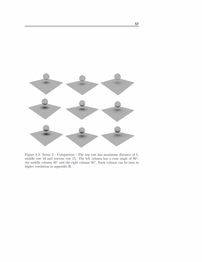
57
Figure 8.2: Scene 2 - Comparison - The top row has maximum distance of 5,middle row 10 and bottom row 15. The left column has a cone angle of 30,the middle column 40 and the right column 50. Each column can be seen inhigher resolution in appendix B.
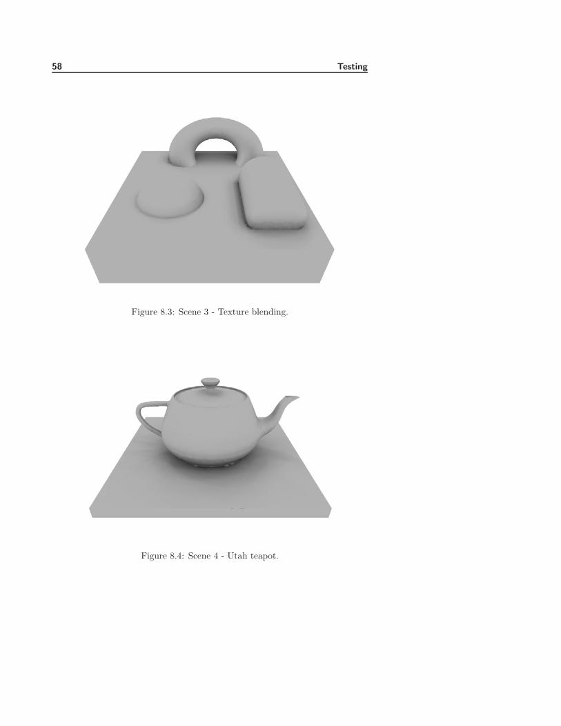
58 Testing
Figure 8.3: Scene 3 - Texture blending.
Figure 8.4: Scene 4 - Utah teapot.
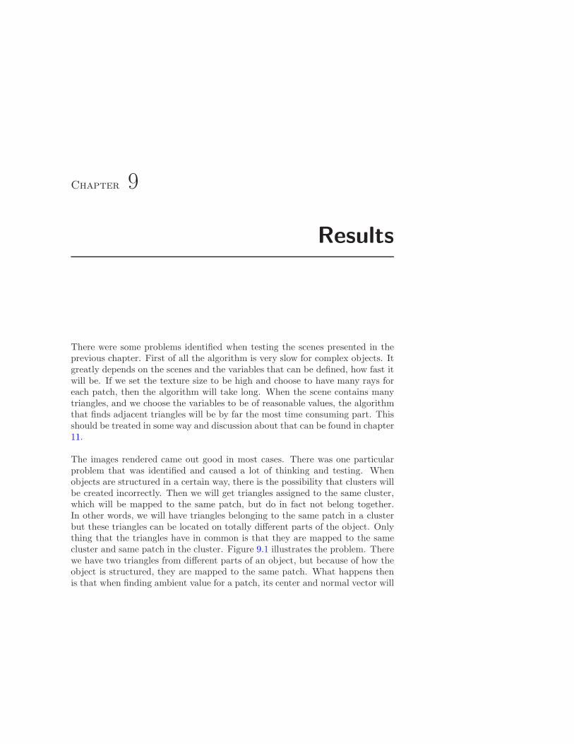
Chapter 9
Results
There were some problems identified when testing the scenes presented in theprevious chapter. First of all the algorithm is very slow for complex objects. Itgreatly depends on the scenes and the variables that can be defined, how fast itwill be. If we set the texture size to be high and choose to have many rays foreach patch, then the algorithm will take long. When the scene contains manytriangles, and we choose the variables to be of reasonable values, the algorithmthat finds adjacent triangles will be by far the most time consuming part. Thisshould be treated in some way and discussion about that can be found in chapter11.
The images rendered came out good in most cases. There was one particularproblem that was identified and caused a lot of thinking and testing. Whenobjects are structured in a certain way, there is the possibility that clusters willbe created incorrectly. Then we will get triangles assigned to the same cluster,which will be mapped to the same patch, but do in fact not belong together.In other words, we will have triangles belonging to the same patch in a clusterbut these triangles can be located on totally different parts of the object. Onlything that the triangles have in common is that they are mapped to the samecluster and same patch in the cluster. Figure 9.1 illustrates the problem. Therewe have two triangles from different parts of an object, but because of how theobject is structured, they are mapped to the same patch. What happens thenis that when finding ambient value for a patch, its center and normal vector will
60 Results
Figure 9.1: Triangles with same patch.
be completely wrong. That is because we take the average of the triangles thatbelong to the patch and the triangles should not all belong to that patch. Thisproblem was identified when the Utah teapot was rendered and is now knownas the teapot problem. In this particular case it works to set the the comparingangle, when clusters are created, to be less than 60. An angle of 57 workedwell which caused the clusters to be smaller and the problem does not presentitself. This works for this case but can easily be created again if an object isstructured in a certain way. Figure 9.2 shows the teapot rendered with differentangles.
Testing shows that memory needed to run the program can be high for largeobjects. This was lowered slightly when the code was optimized, but can still beimproved more. This is mainly when C++ pointer are not released when theyare not in use anymore. The biggest memory usage is when we find ambientocclusion for each patch, when that is done and we have created one texturethat stores the ambient values, the patch clusters are dropped, and memory isreleased.
In general the results indicate that the goal has been achieved. Ambient occlu-sion works as intended for the test scenes, and especially the most importantpart, texture blending is working.
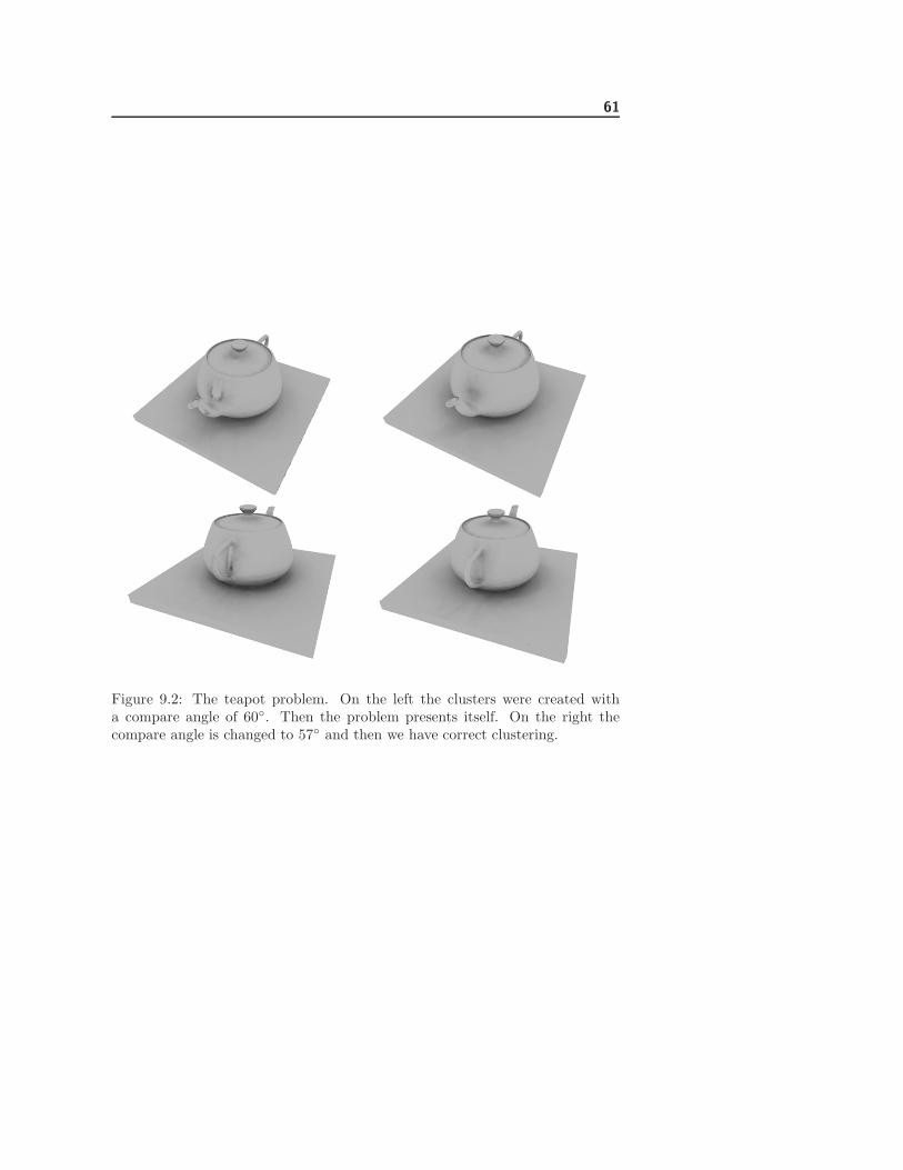
61
Figure 9.2: The teapot problem. On the left the clusters were created witha compare angle of 60. Then the problem presents itself. On the right thecompare angle is changed to 57 and then we have correct clustering.

62 Results
Chapter 10
Discussion
10.1 Summary
The purpose of using ambient occlusion is that we want a more realistic ambientvalue than is presented in the Phong reflection model. There a constant ambientvalue is added to an entire scene. The result of this can be a dull looking imagesince the surrounding environment of a given point on a surface is not considered.Instead we want to consider each point and add a different ambient value to eachone, based on the surrounding environment.
Ambient occlusion adds a subtle but realistic effect to objects and scenes withoutthe need of using a more complex global illumination method. We don’t needto consider any light sources when finding ambient occlusion. This fact canmake development process much easier because developers can apply ambientocclusion and then be able to use less light sources. Also the complication ofplacements of lights will be less because we generally would need fewer lightsources when ambient occlusion has been applied.
Ambient occlusion can be used to simulate other things than just shadows. If thealgorithm is designed in such a way, we can tweak parameters to get interestingresults. This can be for example to simulate dirt or rust that accumulates onobjects or to get a weathered and worn effect. Imagine a statue that has been
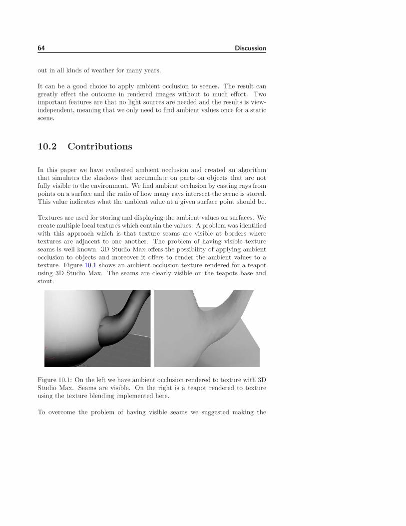
64 Discussion
out in all kinds of weather for many years.
It can be a good choice to apply ambient occlusion to scenes. The result cangreatly effect the outcome in rendered images without to much effort. Twoimportant features are that no light sources are needed and the results is view-independent, meaning that we only need to find ambient values once for a staticscene.
10.2 Contributions
In this paper we have evaluated ambient occlusion and created an algorithmthat simulates the shadows that accumulate on parts on objects that are notfully visible to the environment. We find ambient occlusion by casting rays frompoints on a surface and the ratio of how many rays intersect the scene is stored.This value indicates what the ambient value at a given surface point should be.
Textures are used for storing and displaying the ambient values on surfaces. Wecreate multiple local textures which contain the values. A problem was identifiedwith this approach which is that texture seams are visible at borders wheretextures are adjacent to one another. The problem of having visible textureseams is well known. 3D Studio Max offers the possibility of applying ambientocclusion to objects and moreover it offers to render the ambient values to atexture. Figure 10.1 shows an ambient occlusion texture rendered for a teapotusing 3D Studio Max. The seams are clearly visible on the teapots base andstout.
Figure 10.1: On the left we have ambient occlusion rendered to texture with 3DStudio Max. Seams are visible. On the right is a teapot rendered to textureusing the texture blending implemented here.
To overcome the problem of having visible seams we suggested making the
10.2 Contributions 65
textures overlap and then we find the ambient values as before. This resultsin us getting multiple ambient values on a curved surface which leads to usblending between these values. We blend using the normal vector at the surfaceas the contributing factor. Each of the three normal vector values is used todecide the color of each of the three textures that are overlapping. This givesus smooth blending and less visible texture borders over curved surfaces.

66 Discussion
Chapter 11
Future Work
Following is a discussion about what can be extended or fixed.
The imported geometry data should be represented with simple triangles. Andfurthermore it should be defined in one polygon mesh, meaning we can onlyhave one instance of a mesh declared in the imported COLLADA file. Theseare design decisions. Other types of geometry data could be e.g triangle strips,triangle fans and polygons. There are two possible ways to handle other possi-bilities. Either the implementation should be expanded in such a way that it willhandle these kinds which would not be to much of an effort. Other way would beto create or use a so called conditioner which would convert the kinds mentionedearlier in to the preferred type which would be triangles. Often graphic cardsare optimized in such a way that they are optimized to work fast for trianglestrips. Then it would be preferred to convert all data to triangle strips and thenwork on that. This is not a goal for this kind of work so simple triangles werechosen to work with.
The way adjacent triangles are found is very time consuming. If we have avery complex scene as input, that has many triangles, then this algorithm canbe the most time consuming part of the overall calculations. Usually there isthe need to tweak all the variables for a given scene so that it looks good, andwhen we are experimenting with them, we are always changing the variablesand then running the ambient occlusion on it again. Then this time consuming
68 Future Work
algorithm that finds adjacent triangles can be a broblem. One possibility wouldbe to save the adjacent triangles list in a text file or database and then loadit at runtime. Then we only have to find the adjacency list for the first timefor a given scene. Other possibility would be to allow us to render the scenewith certain parameters, and then change them while rendering to see differentresults. Each triangle knows what triangles are adjacent to him and if we do itlike this, we are working on the same triangles, only changing other parameter.
The physical memory needed for calculating ambient values in complex scenescan be high. This is because in some cases, I have neglected to properly get ridof variables that are not needed anymore, C++ pointers and such. This wasnot a major concern for the implementation, but is still something that needsto be optimized.
Next step would be to apply the ambient occlusion to an object and store theinformation such that it can be used later in a final scene. It would be possibleto create some simple animation with the ambient occlusion applied to theanimated object. Then the algorithm would be applied to each frame in theanimation and stored and then used when the scene is rendered.
The texture packing algorithm is somewhat inefficient. The goal there is tomake sure that the local cluster textures fit in one large texture. The texturesizes are evaluated such that the largest cluster texture is put in first and so on.The packing could be made more efficient by using some well known texturepacking algorithm.
Texture is exported as an uncompressed bitmap image which is an algorithm Iwrote myself. Since bitmaps are uncompressed, at least in this case, the size ofthe texture image can be large. This could be expanded so that the texturesare exported in a different format that supports compression.
There are usually many parts of an object that have no shadows from ambientocclusion. These parts could be evaluated in such a way that they would havemuch smaller part of the ambient texture applied to it, to lower the memoryusage. Same could be done with parts that are highly in shadow or parts wherethere are the same shadow values over a large part. We could lower the texturespace needed for that as well.
It can be a difficult task to find the correct parameters to use for a given scene.The parameters that can have a significant effect on the outcome are the numberof rays to cast, the maximum distance, the cone angle and the texture size inclusters. It would be a good expansion to allow for the user to see visually if hemakes some changes in the parameters. A graphical user interface(GUI) couldbe designed which would load an object with default parameters. Then it would
69
be possible to easily change parameters and the results are shown as soon asthey are ready. This can also have good impact on the part that finds adjacenttriangles since then it would be done when the scene is loaded and stored.
The teapot problem identified in the previous chapter needs to be considered.One possibility would be to look at the location of a triangle when he is beingassigned to a cluster. We would map each triangle to 2D when we are clusteringby dropping the relevant 3D coordinate. Then compare the triangle that we areconsidering now, with all the triangles that have been assigned to the cluster. Ifsome other triangle is located close to this triangle, we compare their values. Ifthe 3D coordinate that was dropped when the triangles were mapped to 2D issignificantly different, we have a triangle that should not belong to this cluster.

70 Future Work
Chapter 12
Conclusion
In this paper we have implemented an algorithm that adds ambient occlusion onobjects. We find the ambient occlusion with help of ray-tracing by shooting outrays from the surface of an object. The number of rays that hit the surroundingenvironment indicates how much shadow that surface point is in.
Figure 12.1 shows a rendered image using the algorithm implemented here. Thescene is a Cornell box. The results from the implementation can also be seenon the figures in chapter 8 - Testing and in appendix B - Screenshots.
There are many possible options at each step when implementing something likehas been done here. Some of the options have been evaluated and discussed,their pros and cons. Many approaches do it similarly as has been done here.That is to trace rays for finding ambient values and use textures to store anddisplay the values. The implementation details vary from designs. The biggestcontribution made in this process has been the overlapping textures and howtheir values are blended in an effort to have seamless textures on surfaces.
We create clusters that consists of all the triangles in the mesh we are workingon. The clusters overlap each other which leads to us finding ambient valuesmore than once for some points on an object. This is done so that we can havea smooth transition between clusters and the overall ambient occlusion will lookrealistic.
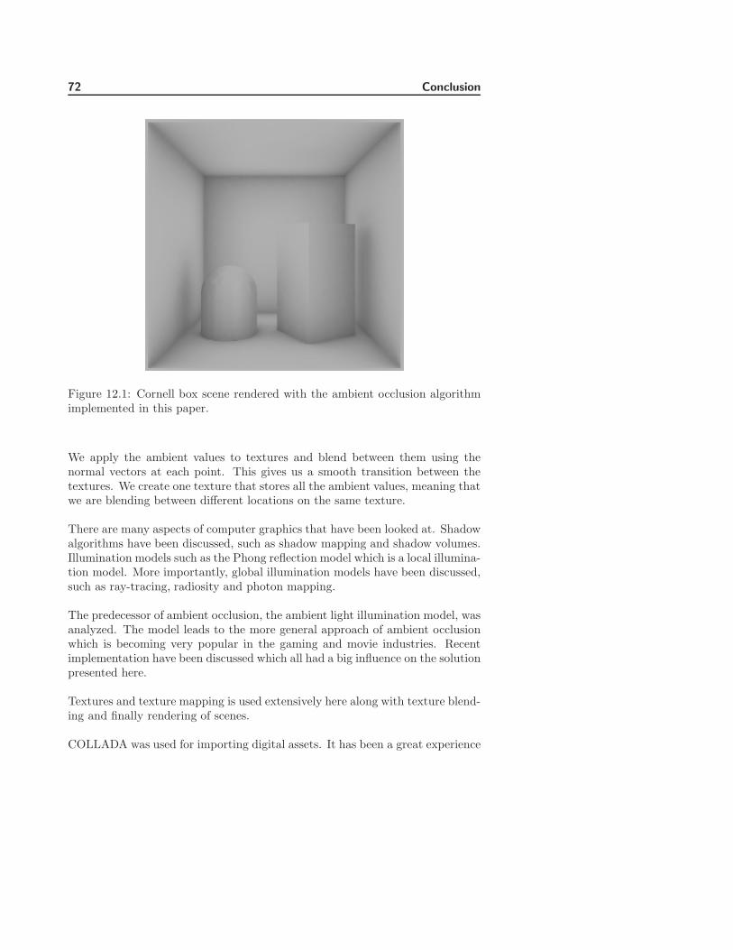
72 Conclusion
Figure 12.1: Cornell box scene rendered with the ambient occlusion algorithmimplemented in this paper.
We apply the ambient values to textures and blend between them using thenormal vectors at each point. This gives us a smooth transition between thetextures. We create one texture that stores all the ambient values, meaning thatwe are blending between different locations on the same texture.
There are many aspects of computer graphics that have been looked at. Shadowalgorithms have been discussed, such as shadow mapping and shadow volumes.Illumination models such as the Phong reflection model which is a local illumina-tion model. More importantly, global illumination models have been discussed,such as ray-tracing, radiosity and photon mapping.
The predecessor of ambient occlusion, the ambient light illumination model, wasanalyzed. The model leads to the more general approach of ambient occlusionwhich is becoming very popular in the gaming and movie industries. Recentimplementation have been discussed which all had a big influence on the solutionpresented here.
Textures and texture mapping is used extensively here along with texture blend-ing and finally rendering of scenes.
COLLADA was used for importing digital assets. It has been a great experience
73
learning about COLLADA, what it stands for and how it is used. COLLADAis an effort in having a common digital asset exchange schema that differentapplications can use. It is being adopted by many companies and for exampleCOLLADA is used in the well known Playstation 3 console from Sony.
The overall process of this thesis has been very informative and most of all fun.There has been a lot of learning and sometimes wrong assumptions made. Whenlooking back at some stages in the process and looking at the assumptions madeat some points, it was clearly easy to go in wrong directions.
When thinking about the options available and the way it was done here, I findthat to be a very interesting idea. The idea of overlapping textures and blendingbetween them using the normal vectors is appealing and can create a realisticsmooth looking images.
We conclude that the goal has been achieved. We have created an algorithm thatcreates multiple overlapping textures on an object and finds ambient values forthe textures. When the object is rendered, the blending occurs on overlappingtextures. The images rendered with this algorithm look smooth and usuallythere are no abrupt shading changes visible.

74 Conclusion
Appendix A
Tools
There are a lot of tools needed to get this kind of project to work. The flow ofthe work relative to the tools used is as follows.
Data is represented in COLLADA[3], and imported into the COLLADA Doc-ument Object Model(DOM)[10]. The COLLADA DOM is an application pro-gramming interface(API) that provides a C++ object orientation of a COL-LADA document. It follows that we will be using C++ for programming sincethe COLLADA DOM was chosen.
To help visualize the implementation, OpenGL[1] was used to a great extent.Also Cg[14] has been used to create a fragment program that allow us to usehardware to calculate values.
Softimage|XSI was used for creating objects and scenes for testing.
A.1 COLLADA
COLLADA stands for COLLAborative Design Activity which defines an XML-based schema to enable 3-D authoring applications to freely exchange digitalassets without loss of information[3]. It was created through the collaboration
76 Appendix A
of many companies and was adopted as an official industry standard by theKhronos group in January 2006. COLLADA is supported by many tools andis already used by thousands of developers. COLLADA is very young. AfterSIGGRAPH ’03, Sony Computer Entertainment, established a working group,which did a thorough analysis of all existing digital asset formats. Many othercompanies in the gaming industry became involved and at SIGGRAPH ’04the first public presentation of COLLADA 1.0 was made. Since then it hasgone through revisions and current version is 1.4.1. COLLADA has many goalsincluding to be used as a common data exchange, be adopted by many digital-content users and provide an easy integration mechanism which enables all datato be available through COLLADA. It also has the goal of liberating digitalassets from binary formats which is why it was chosen to be an XML-basedschema. Arnaud and Barnes have written a book[2] which covers all aspects ofCOLLADA.
A.2 COLLADA DOM
To be able to interact with the data in a COLLADA file, the COLLADA Doc-ument Object Model[10] will be used. The DOM is a framework to be used forthe development of COLLADA applications. It provides a C++ programminginterface to load, query and translate instance data. The DOM loads the datainto a runtime database which mirrors those defined in the COLLADA schema.
A.3 Softimage XSI
Softimage|XSI is a 3D animation and modeling software. Many models usedin this report were created with Softimage. Softimage has the possibility ofexporting scenes as a COLLADA schema. It has the option of converting allgeometry to triangles before exporting, which is convenient for the implemen-tation. When a scene is created in Softimage that we want to find ambientocclusion for using the algorithm presented here, we first need to convert allmeshes into one polygon mesh object. Then that one object should be exportedas that are the requirements in the implementation.
A.4 OpenGL and Cg 77
A.4 OpenGL and Cg
The implementation requires constant visual representation to see what is goingon and OpenGl[1] is great for that since it allows for a fast visual representationof the data whenever needed. OpenGL stands for Open Graphics Library andis a software interface to graphics hardware. It consists of procedures and func-tions that allow a programmer to specify objects and operations for producinggraphical images. Cg[14] stands for C for graphics. The Cg language allows forcontrol of objects, their shape, appearance and motion which will be renderedusing graphics hardware. This means that Cg allows us to program the graphicshardware directly without going into the hardware assembly language. In thisparticular case Cg is used to blend between different locations on a texture.A Cg fragment program is created which input is a pixel color, three texturecolors, possibly from different places on one texture, and the normal vector atthe given point. Each texture color is multiplied with one of the normal vectorvalues and the colors are then added together. The output is then the inputcolor multiplied with the texture colors.

78
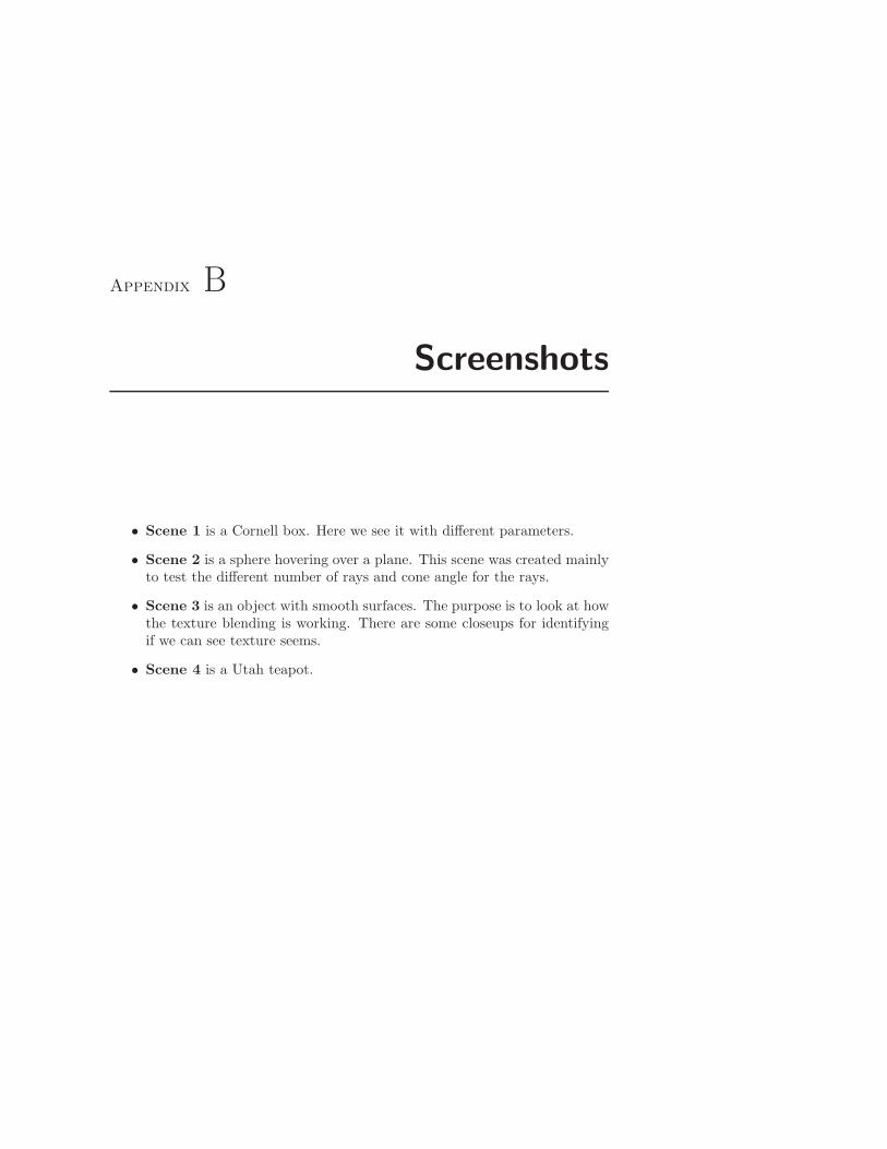
Appendix B
Screenshots
• Scene 1 is a Cornell box. Here we see it with different parameters.
• Scene 2 is a sphere hovering over a plane. This scene was created mainlyto test the different number of rays and cone angle for the rays.
• Scene 3 is an object with smooth surfaces. The purpose is to look at howthe texture blending is working. There are some closeups for identifyingif we can see texture seems.
• Scene 4 is a Utah teapot.
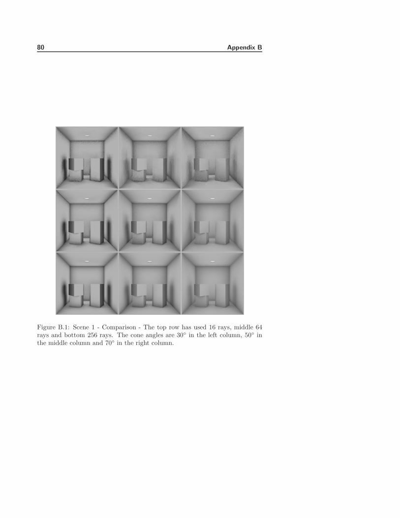
80 Appendix B
Figure B.1: Scene 1 - Comparison - The top row has used 16 rays, middle 64rays and bottom 256 rays. The cone angles are 30 in the left column, 50 inthe middle column and 70 in the right column.

Screenshots 81
Figure B.2: Scene 1 - Comparison - The cone angle is 20. The top has 16 rays,middle 64 rays and bottom 256 rays.
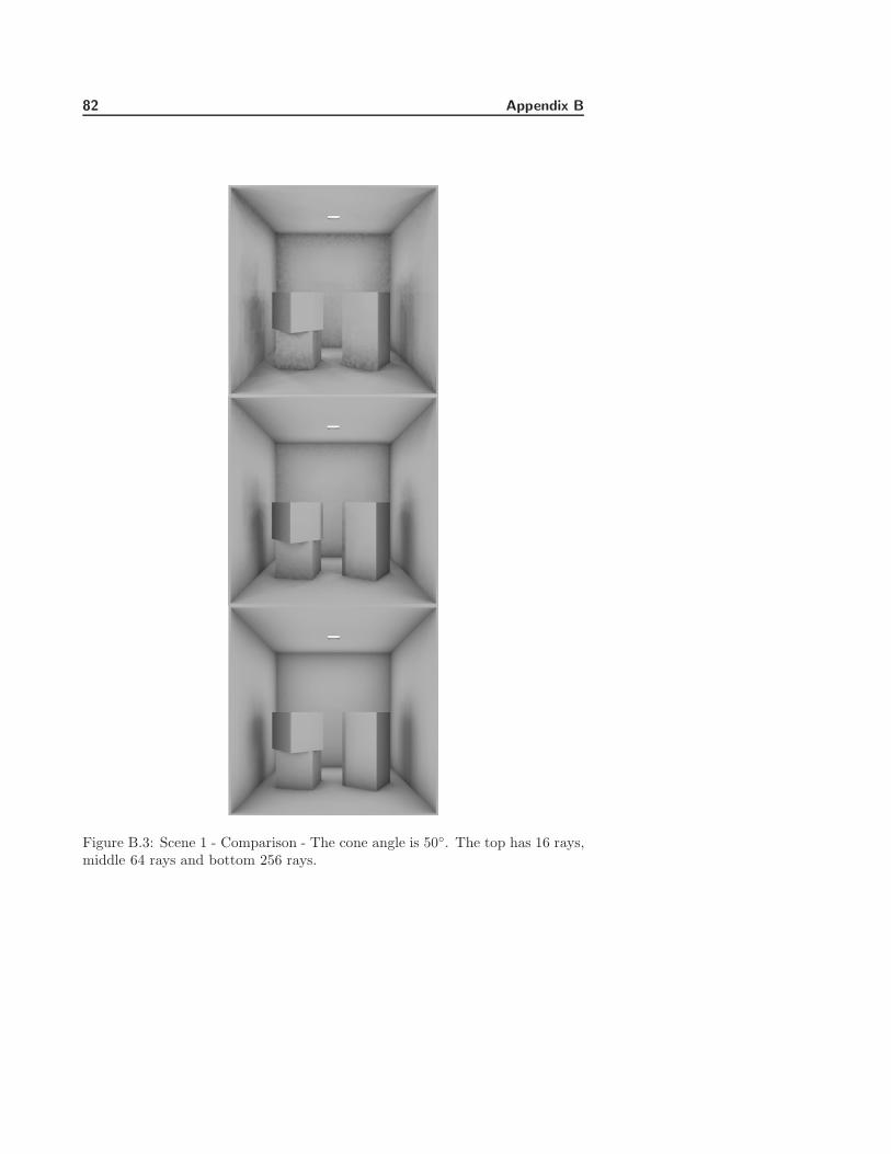
82 Appendix B
Figure B.3: Scene 1 - Comparison - The cone angle is 50. The top has 16 rays,middle 64 rays and bottom 256 rays.
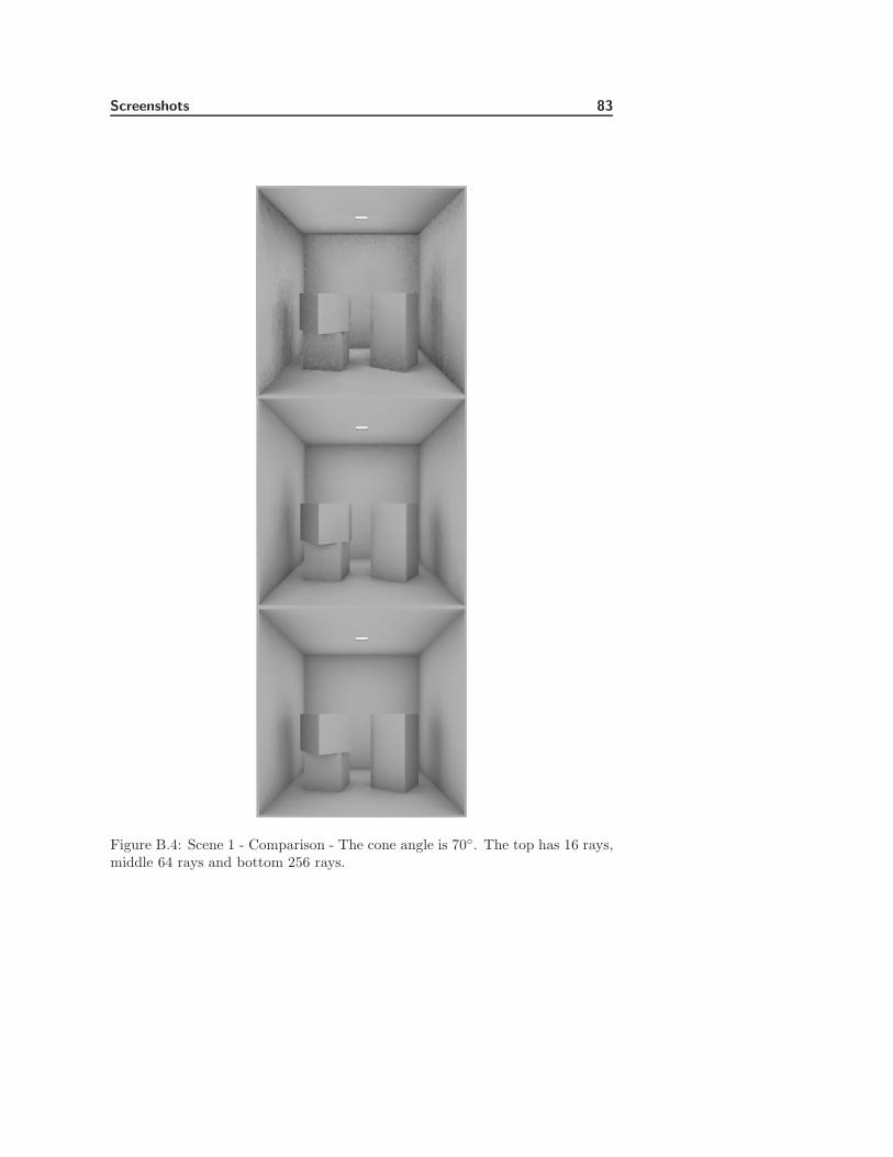
Screenshots 83
Figure B.4: Scene 1 - Comparison - The cone angle is 70. The top has 16 rays,middle 64 rays and bottom 256 rays.
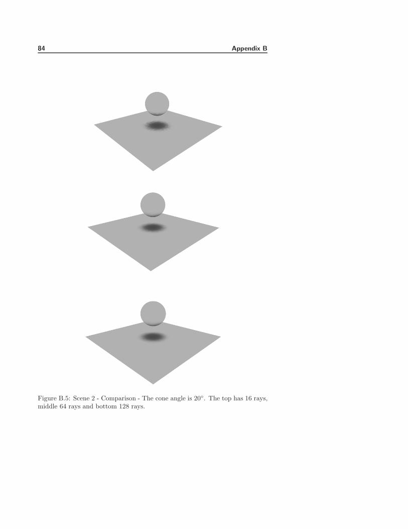
84 Appendix B
Figure B.5: Scene 2 - Comparison - The cone angle is 20. The top has 16 rays,middle 64 rays and bottom 128 rays.
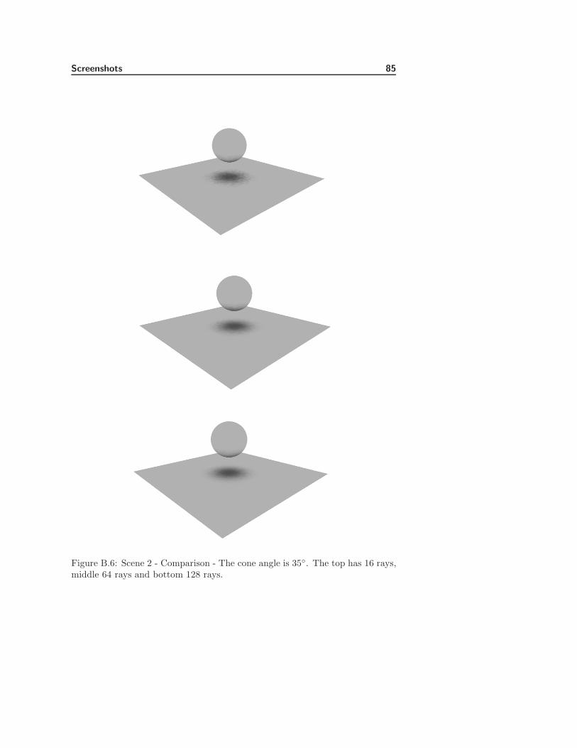
Screenshots 85
Figure B.6: Scene 2 - Comparison - The cone angle is 35. The top has 16 rays,middle 64 rays and bottom 128 rays.
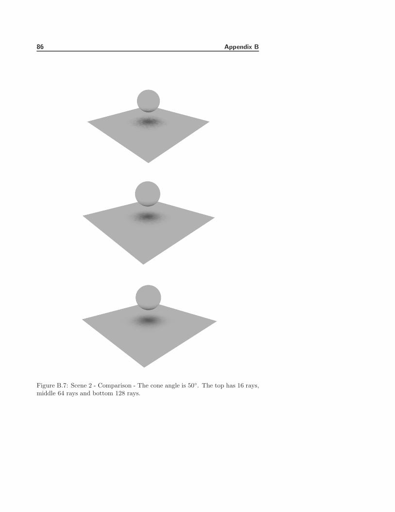
86 Appendix B
Figure B.7: Scene 2 - Comparison - The cone angle is 50. The top has 16 rays,middle 64 rays and bottom 128 rays.
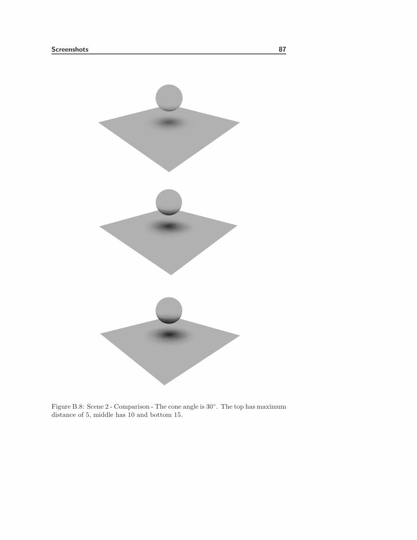
Screenshots 87
Figure B.8: Scene 2 - Comparison - The cone angle is 30. The top has maximumdistance of 5, middle has 10 and bottom 15.
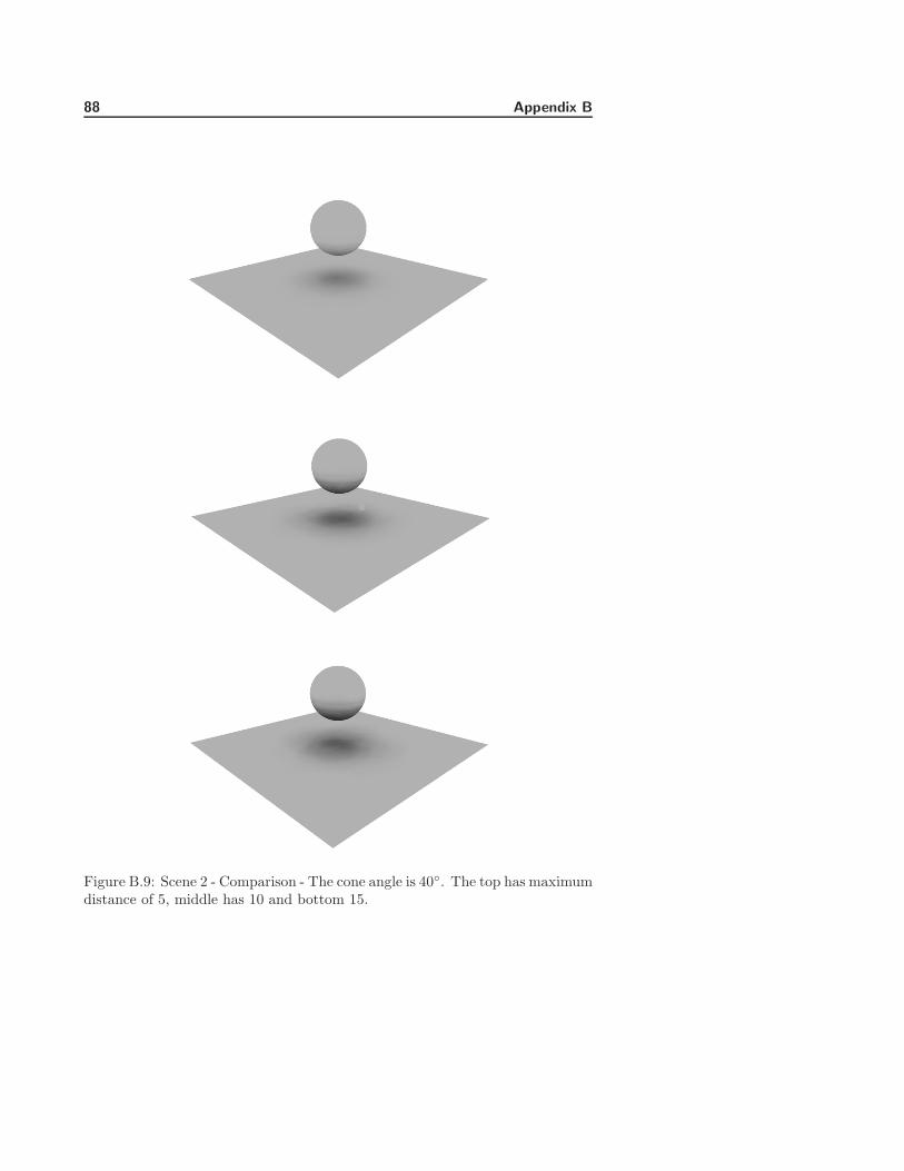
88 Appendix B
Figure B.9: Scene 2 - Comparison - The cone angle is 40. The top has maximumdistance of 5, middle has 10 and bottom 15.

Screenshots 89
Figure B.10: Scene 2 - Comparison - The cone angle is 50. The top hasmaximum distance of 5, middle has 10 and bottom 15.

90 Appendix B
Figure B.11: Scene 3.
Figure B.12: Scene 3.
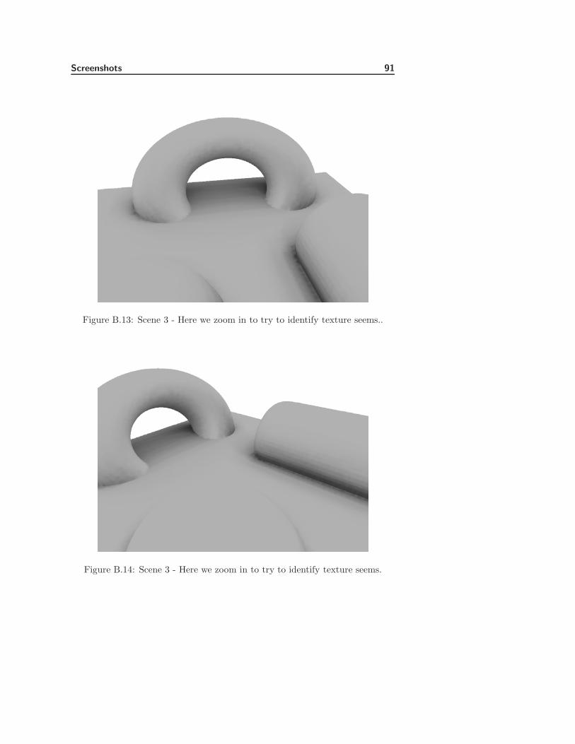
Screenshots 91
Figure B.13: Scene 3 - Here we zoom in to try to identify texture seems..
Figure B.14: Scene 3 - Here we zoom in to try to identify texture seems.
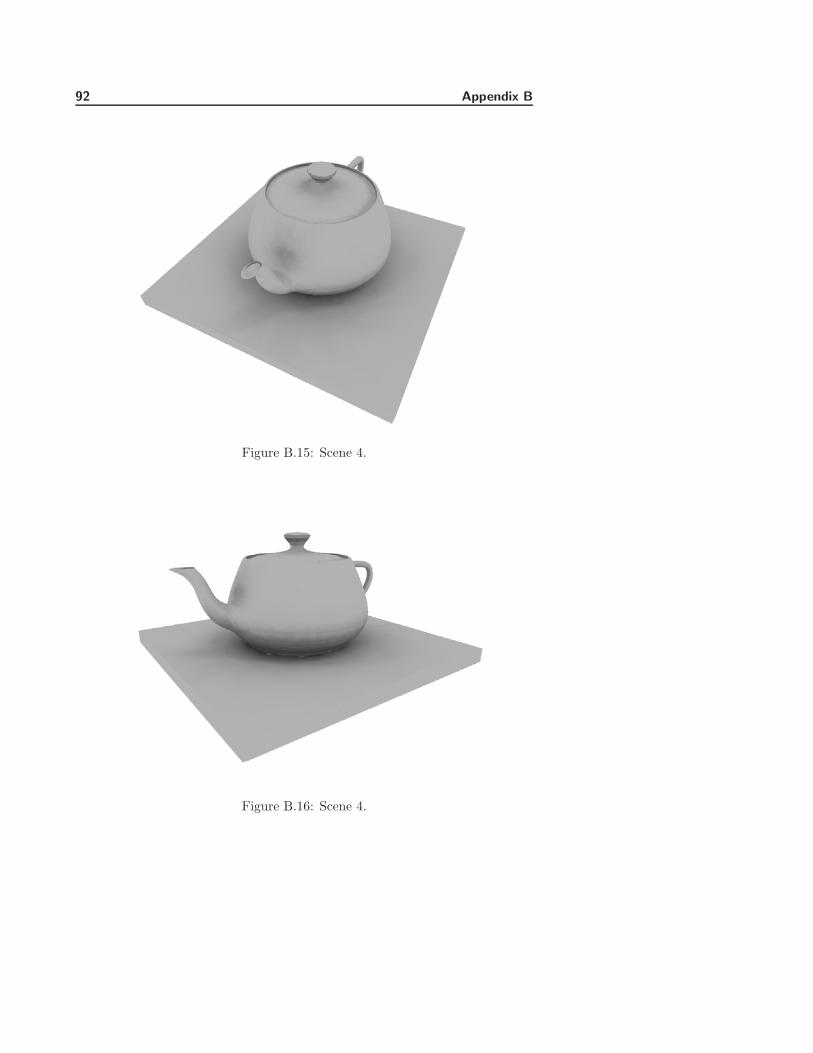
92 Appendix B
Figure B.15: Scene 4.
Figure B.16: Scene 4.
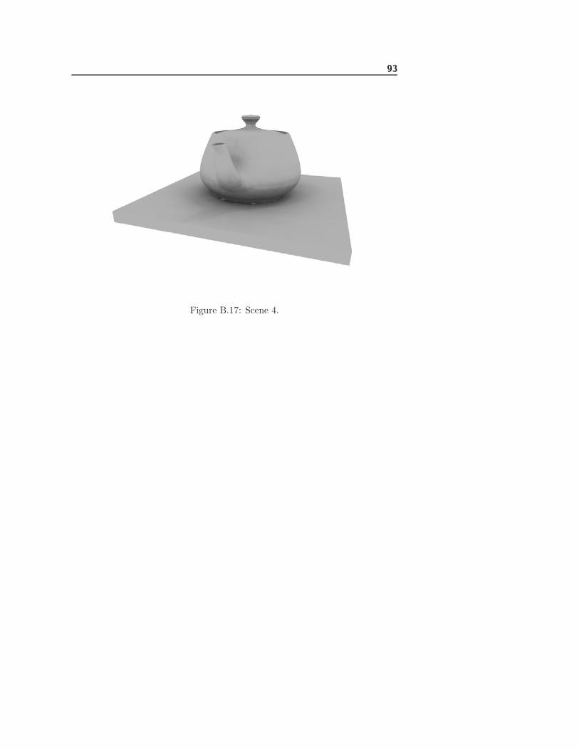
93
Figure B.17: Scene 4.

94
Bibliography
[1] Akeley K., Segal M., The OpenGL Graphics System: A Specification, Ver-sion 2.1, July 30, 2006.
[2] Arnaud R., Barnes M.C., COLLADA Sailing the Gulf of 3D Digital ContentCreation, A K Peters, Ltd. 2006.
[3] Barnes M. Ed., COLLADA - Digital Asset Schema Release 1.4.1 Specifica-tion, Sony Computer Entertainment Inc., June, 2006.
[4] Bunnell M., Dynamic Ambient Occlusion and Indirect Lighting, GPU Gems2, Chapter 14, pp. 223-233, NVIDIA Corporation, 2005.
[5] Borshukov G., Piponi D., Seamless Texture Mapping of Subdivision Sur-faces by Model Pelting and Texture Blending, MVFX, a division of ManexEntertainment.
[6] Castro F., Neumann L. and Sbert M., “Extended Ambient Term,” in Journalof Graphics Tools, vol. 5, no. 4, pp. 1-7, November, 2000.
[7] Catmull E., A Subdivision Algorithm for the Computer Display of CurvedSurfaces, PhD thesis, University of Utah, December, 1974.
[8] Chan E., Durand F., “An Efficient Hybrid Shadow Rendering Algorithm,”in Proceedings of the Eurographics Symposium on Rendering, EurographicsAssociation, pp. 185-195, 2004.
[9] Christensen P. H., “Global Illumination and all that,” in Siggraph 2003course 9: Renderman, Theory and Practice, Batall D. Ed., ACM Siggraph,pp. 31-72, 2003.
96 BIBLIOGRAPHY
[10] COLLADA DOM 1.4.0 - Programming Guide, Sony Computer Entertain-ment Inc., 2006.
[11] Cormen T. H., Leiserson C. E., Rivest R. L., Stein C., Introduction toAlgorithms, Second Edition, McGraw-Hill Book Company, 2001.
[12] Crow F. C., “Shadow Algorithms for Computer Graphics,” in SIGGRAPH’77: Proceedings of the 4th annual conference on Computer graphics andinteractive techniques, pp. 242-248, 1977.
[13] Everitt C., “Interactive Order-Independent Transparency,” Technical Re-port, NVIDIA Corporation, 2001.
[14] Fernando R., Kilgard M. J., The Cg Tutorial, The Definitive Guide toProgrammable Real-Time Graphics, NVidia Corporation, Addison-Wesley.
[15] Goral, C. M., Torrance, K. E., Greenberg, D. P. and Battaile, B., “Modelingthe Interaction of Light Between Diffuse Sources,” in Proceedings of the11th Annual Conference on Computer Graphics and Interactive Techniques,SIGGRAPH ’84. ACM Press, New York, NY, pp. 213-222, 1984.
[16] Hasenfratz J. M., Lapierre M., Holzschuch N. and Sillion E., “A Survey ofReal-time Soft Shadows Algorithms,” in Computer Graphics Forum, vol. 22,no. 4 pp: 753-774, 2003.
[17] Iones A., Krupkin A., Sbert M. and Zhukov A., “Fast Realistic Lightingfor Video Games,” in IEEE Computer Graphics and Applications, vol. 23,no. 3, pp. 54-64, May 2003.
[18] Jensen H. W., “Global Illumination Using Photon Maps,” in RenderingTechniques ’96, Pueyo X. and Schroder P. Eds., Springer-Verlag, pp. 21-30,1996.
[19] Kontkanen J. and Laine S., “Ambient Occlusion Fields,” in Proceedings ofACM SIGGRAPH 2005 Symposium on Interactive 3D Graphics and Games,ACM Press, pp. 41-48, 2005.
[20] Landis H., “Production-Ready Global Illumination,” in SIGGRAPH 2002,course notes #16 (Renderman in Production), pp. 87-102, ACM, July 2002.
[21] Malmer M., Malmer F., Assarsson U. and Holzschuch N., “Fast Precom-puted Ambient Occlusion for Proximity Shadows,” in Journal of GraphicsTools, 2006.
[22] Mendez-Feliu A., Sbert M., Cata J., Sunyer N. and Funtane S., “Real-time Obscurances with Color Bleeding,” in Proceedings of the 19th springconference on Computer graphics, Szirmay-Kalos L., Ed. SCCG ’03. ACMPress, New York, NY, pp. 171-176, 2003.
BIBLIOGRAPHY 97
[23] Phong B. T., “Illumination for Computer Generated Pictures,” in Com-munications of the ACM, vol. 18, no. 6, pp. 311-317, June 1975.
[24] Watt A., Watt M., Advanced Animation and Rendering Techniques. The-ory and Practice, Addison-Wesley, 1992.
[25] Whitted T., “An Improved Illumination Model for Shaded Display,” inCommunications of the ACM, vol. 23, no. 6, pp.343-349, June 1980.
[26] Williams L., “Casting Curved Shadows on Curved Surfaces,” ComputerGraphics Lab, New York Institute of Technology, Old Westbury, New York,1978.
[27] Woo A., Poulin P., Fournier A., “A Survey of Shadow Algorithms,” in IEEEComputer Graphics and Applications, vol. 10, no. 6, pp. 13-32, November1990.
[28] Zhukov S., Iones A., Kronin G., “An Ambient Light Illumination Model,”in Rendering Techniques ’98, Drettakis G. and Max N., Eds., pp. 45-56, 1998.