
amath582
209
AMATH 582 Computation Methods for Data Analysis ∗ J. Nathan Kutz † March 30, 2011 Abstract This course is a survey of computational methods used for extracting meaningful results out of experimental or computational data. The cen- tral focus is on using a combination of spectral methods, statistics and linear algebra to analyze data and determine trends which are statistically significant. * These notes are intended as the primary source of information for AMATH 582. The notes are incomplete and may contain errors. Any other use aside from classroom purposes and personal research please contact me at [email protected]. c J.N.Kutz, Winter 2010 (Version 1.0) † Department of Applied Mathematics, Box 352420, University of Washington, Seattle, WA 98195-2420 ([email protected]). 1
-
Upload
joekurina3194 -
Category
Documents
-
view
29 -
download
0
description
uw applied math 582 text
Transcript of amath582

AMATH 582
Computation Methods for
Data Analysis∗
J. Nathan Kutz†
March 30, 2011
Abstract
This course is a survey of computational methods used for extracting
meaningful results out of experimental or computational data. The cen-
tral focus is on using a combination of spectral methods, statistics and
linear algebra to analyze data and determine trends which are statistically
significant.
∗These notes are intended as the primary source of information for AMATH 582. Thenotes are incomplete and may contain errors. Any other use aside from classroom purposesand personal research please contact me at [email protected]. c©J.N.Kutz, Winter2010 (Version 1.0)
†Department of Applied Mathematics, Box 352420, University of Washington, Seattle, WA98195-2420 ([email protected]).
1

AMATH 582 ( c©J. N. Kutz) 2
Contents
1 Statistical Methods and Their Applications 41.1 Basic probability concepts . . . . . . . . . . . . . . . . . . . . . . 41.2 Random variables and statistical concepts . . . . . . . . . . . . . 111.3 Hypothesis testing and statistical significance . . . . . . . . . . . 20
2 Time-Frequency Analysis: Fourier Transforms and Wavelets 262.1 Basics of Fourier Series and the Fourier Transform . . . . . . . . 272.2 FFT Application: Radar Detection and Filtering . . . . . . . . . 352.3 FFT Application: Radar Detection and Averaging . . . . . . . . 422.4 Time-Frequency Analysis: Windowed Fourier Transforms . . . . 492.5 Time-Frequency Analysis and Wavelets . . . . . . . . . . . . . . 562.6 Multi-Resolution Analysis and the Wavelet Basis . . . . . . . . . 642.7 Spectrograms and the Gabor transforms in MATLAB . . . . . . 692.8 MATLAB Filter Design and Wavelet Toolboxes . . . . . . . . . . 75
3 Image Processing and Analysis 813.1 Basic concepts and analysis of images . . . . . . . . . . . . . . . 823.2 Linear filtering for image denoising . . . . . . . . . . . . . . . . . 893.3 Diffusion and image processing . . . . . . . . . . . . . . . . . . . 95
4 Linear Algebra and Singular Value Decomposition 1014.1 Basics of The Singular Value Decomposition (SVD) . . . . . . . . 1014.2 The SVD in broader context . . . . . . . . . . . . . . . . . . . . . 1074.3 Introduction to Principle Component Analysis (PCA) . . . . . . 1134.4 Principal Components, Diagonalization and SVD . . . . . . . . . 1184.5 Principal Components and Proper Orthogonal Models . . . . . . 121
5 Independent Component Analysis 1305.1 The concept of independent components . . . . . . . . . . . . . . 1305.2 Image separation problem . . . . . . . . . . . . . . . . . . . . . . 1375.3 Image separation and MATLAB . . . . . . . . . . . . . . . . . . 144
6 Image Recognition 1496.1 Recognizing dogs and cats . . . . . . . . . . . . . . . . . . . . . . 1496.2 The SVD and Linear Discrimination Analysis . . . . . . . . . . . 1566.3 Implementing cat/dog recognition in MATLAB . . . . . . . . . . 165
7 Dimensionality Reduction for Partial Differential Equations 1697.1 Modal expansion techniques for PDEs . . . . . . . . . . . . . . . 1697.2 PDE dynamics in the right (best) basis . . . . . . . . . . . . . . 1757.3 Global normal forms of bifurcation structures in PDEs . . . . . . 180

AMATH 582 ( c©J. N. Kutz) 3
8 Equation Free Modeling 1918.1 Multi-scale physics: an equation-free approach . . . . . . . . . . 1918.2 Lifting and restricting in equation-free computing . . . . . . . . . 1968.3 Equation-free space-time dynamics . . . . . . . . . . . . . . . . . 203

AMATH 582 ( c©J. N. Kutz) 4
1 Statistical Methods and Their Applications
Our ultimate goal is to analyze highly generic data arising from applications asdiverse as imaging, biological sciences, atmospheric sciences, or finance, to namea few specific examples. In all these application areas, there is a fundamentalreliance on extracting meaningful trends and information from large data sets.Primarily, this is motivated by the fact that in many of these systems, thedegree of complexity, or the governing equations, are unknown or impossible toextract. Thus one must rely on data, its statistical properties, and its analysisin the context of spectral methods and linear algebra.
1.1 Basic probability concepts
To understand the methods required for data analysis, a review of probabilitytheory and statistical concepts is necessary. Many of the ideas presented in thissection are intuitively understood to most students in the mathematical, biolog-ical, physical and engineering sciences. Regardless, a review will serve to refreshone with the concepts and will further help understand their implementation inMATLAB.
Sample space and events
Often one performs an experiment whose outcome is not known in advance.However, while the outcome is not known, suppose that the set of all possibleoutcomes is known. The set of all possible outcomes is the sample space of theexperiment and is denoted by S. Some specific examples of sample spaces arefollowing:
1. If the experiment consists of flipping a coin, then
S = {H,T }where H denotes an outcome of heads and T denotes an outcome of tails.
2. If the experiment consists of flipping two coins, then
S = {(H,H), (H,T ), (T,H), (T, T )}where the outcome (H,H) denotes both coins being heads, (H,T ) denotesthe first coin being heads and the second tails, (T,H) denotes the first coinbeing tails and the second being heads, and (T, T ) denotes both coins beingtails.
3. If the experiment consists of tossing a die, then
S = {1, 2, 3, 4, 5, 6}where the outcome i means that the number i appeared on the die, i =1, 2, 3, 4, 5, 6.
AMATH 582 ( c©J. N. Kutz) 5
Any subset of the sample space is referred to as an event, and it is denotedby E. For the sample spaces given above, we can also define an event.
1. If the experiment consists of flipping a single coin, then
E = {H}
denotes the event that a head appears on the coin.
2. If the experiment consists of flipping two coins, then
E = {(H,H), (H,T )}
denotes the event where a head appears on the first coin .
3. If the experiment consists of tossing a die, then
E = {2, 4, 6}
would be the event that an even number appears on the toss.
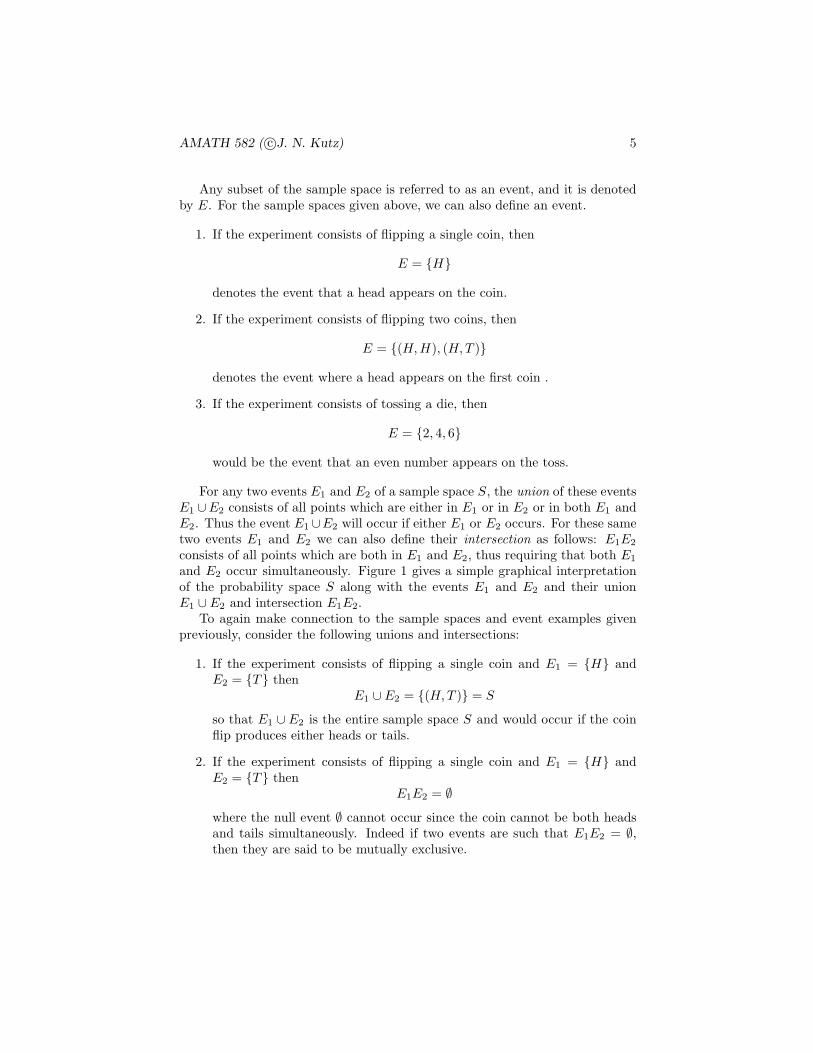
For any two events E1 and E2 of a sample space S, the union of these eventsE1 ∪E2 consists of all points which are either in E1 or in E2 or in both E1 andE2. Thus the event E1 ∪E2 will occur if either E1 or E2 occurs. For these sametwo events E1 and E2 we can also define their intersection as follows: E1E2
consists of all points which are both in E1 and E2, thus requiring that both E1
and E2 occur simultaneously. Figure 1 gives a simple graphical interpretationof the probability space S along with the events E1 and E2 and their unionE1 ∪ E2 and intersection E1E2.
To again make connection to the sample spaces and event examples givenpreviously, consider the following unions and intersections:
1. If the experiment consists of flipping a single coin and E1 = {H} andE2 = {T } then
E1 ∪ E2 = {(H,T )} = S
so that E1 ∪ E2 is the entire sample space S and would occur if the coinflip produces either heads or tails.
2. If the experiment consists of flipping a single coin and E1 = {H} andE2 = {T } then
E1E2 = ∅where the null event ∅ cannot occur since the coin cannot be both headsand tails simultaneously. Indeed if two events are such that E1E2 = ∅,then they are said to be mutually exclusive.

AMATH 582 ( c©J. N. Kutz) 6
Figure 1: Venn diagram showing the sample space S along with the events E1
and E2. The union of the two events E1 ∪ E2 is denoted by the gray regionswhile the intersection E1E2 is depicted in the cross-hatched region where thetwo events overlap.
3. If the experiment consists of tossing a die and if E1 = {1, 3, 5} and E2 ={1, 2, 3} then
E1E2 = {1, 3}so that the intersection of these two events would be a roll of the die ofeither 1 or 3.
The union and intersection of more than two events can be easily generalizedfrom these ideas. Consider a set of events E1, E2, · · · , EN , then the union isdefined as ∪Nn=1En = E1 ∪ E2 ∪ · · · ∪ EN and the intersection is defined as∏Nn=1 En = E1E2 · · ·EN . Thus an event which is in any of the En belongs
to the union whereas an even needs to be in all En in order to be part of theintersection (n = 1, 2, · · · , N). The compliment of an event E, denoted Ec,consists of all points in the sample space S not in E. Thus E ∪ Ec = S andEEc = ∅.
Probabilities defined on events
With the concept of sample spaces S and events E in hand, the probability ofan event P (E) can be calculated. Thus the following conditions are necessaryin defining a number to P (E):

AMATH 582 ( c©J. N. Kutz) 7
• 0 ≤ P (E) ≤ 1
• P (S) = 1
• For any sequence of events E1, E2, · · ·EN that are mutually exclusive sothat EiEj = ∅ when i 6= j then
P(∪Nn=1En
)=
N∑
n=1
P (En)
The notation P (E) is the probability of the event E occurring. The concept ofprobability is quite intuitive and it can be quite easily applied to our previousexamples.
1. If the experiment consists of flipping a fair coin, then
P ({H}) = P ({T }) = 1/2
where H denotes an outcome of heads and T denotes an outcome of tails.On the other hand, a biased coin that was twice as likely to produce headsover tails would result in
P ({(H}) = 2/3, P ({T }) = 1/3
2. If the experiment consists of flipping two fair coins, then
P ({(H,H)} = 1/4
where the outcome (H,H) denotes both coins being heads.
3. If the experiment consists of tossing a fair die, then
P ({1}) = P ({2}) = P ({3}) = P ({4}) = P ({5}) = P ({6}) = 1/6
and the probability of producing an even number
P ({2, 4, 6}) = P ({2}) + P ({4}) + P ({6}) = 1/2.
This is a formal definition of the probabilities being functions of events on samplespaces. On the other hand, our intuitive concept of the probability is that if anevent is repeated over and over again, then with probability one, the proportionof time and event E occurs is just P (E). This is the frequentists viewpoint.
A few more facts should be placed here. First, since E and Ec are mutuallyexclusive and E ∪ Ec = S, then P (S) = P (E ∪ Ec) = P (E) + P (Ec) = 1.Additionally, we can compute the formula for P (E1∪E2) which is the probabilitythat either E1 or E2 occurs. From Fig. 1 it can be seen that the probability

AMATH 582 ( c©J. N. Kutz) 8
P (E1) + P (E2), which represents all points in E1 and all points in E2, is givenby the gray regions. Notice in this calculation, that the overlap region is countedtwice. Thus the intersection must be subtracted so that we find
P (E1 ∪ E2) = P (E1) + P (E2) − P (E1E2) . (1.1.1)
If the two events E1 and E2 are mutually exclusive then E1E2 = ∅ and P (E1 ∪E2) = P (E1) + P (E2) (Note that P (∅) = 0).
As an example, consider tossing two fair coins so that each of the pointsin the sample space S = {(H,H), (H,T ), (T,H), (T, T )} is equally likely tooccur, or said another way, each has probability of 1/4 to occur. Then letE1 = {(H,H), (H,T )} be the event where the first coin is a heads, and letE2 = {(H,H), (T,H)} be the event that the second coin is a heads. Then
P (E1 ∪E2) = P (E1) + P (E2) − P (E1E2)
=1
2+
1
2− P{(H,H)} =
1
2+
1
2− 1
4=
3
4
Of course, this could have also easily been computed directly from the unionP (E1 ∪ E2) = P ({(H,H), (H,T ), (T,H)}) = 3/4.
Conditional probabilities
Conditional probabilities concerns, in some sense, the interdependency of events.Specifically, given that the event E1 has occurred, what is the probability of E2
occurring. This conditional probability is denoted as P (E2|E1). A general for-mula for the conditional probability can derived from the following argument: Ifthe event E1 occurs, then in order for E2 to occur, it is necessary that the actualoccurrence be in the intersection E1E2. Thus in the conditional probability wayof thinking, E1 becomes our new sample space, and the event that E1E2 occurswill equal the probability of E1E2 relative to the probability of E1. Thus wehave the conditional probability definition
P (E2|E1) =P (E2E1)
P (E1). (1.1.2)
The following are examples of some basic conditional probability events.
1. If the experiment consists of flipping two fair coins, what is the probabilitythat both are heads given that at least one of them is heads? With thesample space S = {(H,H), (H,T ), (T,H), (T, T )} and each outcome aslikely to occur as the other. Let E2 denote the event that both coins areheads, and E1 denote the event that at least one of them is heads, then
P (E2|E1) =P (E2E1)
P (E1)=
P ({(H,H)})P ({(H,H), (H,T ), (T,H)}) =
1/4
3/4=
1
3

AMATH 582 ( c©J. N. Kutz) 9
2. Suppose cards numbered one through ten are placed in a hat, mixed anddrawn. If we are told that the number on the drawn card is at leastfive, then what is the probability that it is ten? In this case, E2 is theprobability (= 1/10) that the card is a ten, while E1 is the probability(= 6/10) that it is at least a five. then
P (E2|E1) =1/10
6/10=
1
6.
Independent events
Independent events will be of significant interest in this course. More specifically,the definition of independent events determines whether or not an event E1 hasany impact, or is correlated, with a second event E2. By definition, two eventsare said to be independent if
P (E1E2) = P (E1)P (E2) . (1.1.3)
By Equation (1.1.2), this implies that E1 and E2 are independent if
P (E2|E1) = P (E2) . (1.1.4)
In other words, the outcome of obtaining E2 does not depend upon whether E1
occurred. Two events that are not independent are said to be dependent.As an example, consider tossing two fair die where each possible outcome is
an equal 1/36. Then let E1 denote the event that the sum of the dice is six, E2
denote the event that the first die equals four and E3 denote the event that thesum of the dice is seven. Note that
P (E1E2) = P ({(4, 2)}) = 1/36
P (E1)P (E2) = 5/36 × 1/6 = 5/216
P (E3E2) = P ({(4, 3)}) = 1/36
P (E3)P (E2) = 1/6 × 1/6 = 1/36
Thus we can find that E2 and E1 cannot be independent while E3 and E2 are,in fact, independent. Why is this true? In the first case where a total of six(E2) on the die is sought, then the roll of the first die is important as it must bebelow six in order to satisfy this condition. On the other hand, a total of sevencan be accomplished (E3) regardless of the first die roll.
Bayes’s Formula
Consider two events E1 and E2. Then the event E1 can be expressed as follows
E1 = E1E2 ∪ E1Ec2 . (1.1.5)
AMATH 582 ( c©J. N. Kutz) 10
This is true since in order for a point to be in E1, it must either be in E1 andE2, or it must be in E1 and not in E2. Since the intersections E1E2 and E1E
c2
are obviously mutually exclusive, then
P (E1) = P (E1E2) + P (E1Ec2)
= P (E1|E2)P (E2) + P (E1|Ec2)P (Ec2)
= P (E1|E2)P (E2) + P (E1|Ec2)(1 − P (E2)) (1.1.6)
This states that the probability of the event E1 is a weighted average of theconditional probability of E1 given that E2 has occurred and the conditionalprobability of E1 given that E2 has not occurred, with each conditional prob-ability being given as much weight as the event it is conditioned on has ofoccurring. To illustrate the application of Bayes’s formula, consider the twofollowing examples:
1. Consider two boxes: the first containing two white and seven black balls,and the second containing five white and six black balls. Now flip a faircoin and draw a ball from the first or second box depending on whether youget heads or tails. What is the conditional probability that the outcome ofthe toss was heads given that a white ball was selected? For this problem,letW be the event that a white ball was drawn andH be the event that thecoin came up heads. The solution to this problem involves the calculationof P (H |W ). This can be calculated as follows:
P (H |W ) =P (HW )
P (W )=P (W |H)P (H)
P (W )
=P (W |H)P (H)
P (W |H)P (H) + P (W |Hc)P (Hc)
=2/9 × 1/2
2/9 × 1/2 + 5/11 × 1/2=
22
67(1.1.7)
2. A laboratory blood test is 95% effective in determining a certain diseasewhen it is present. However, the test also yields a false positive result for1% of the healthy persons tested. If 0.5% of the population actually hasthe disease, what is the probability a person has the disease given thattheir test result is positive? For this problem, let D be the event that theperson tested has the disease, and E the event that their test is positive.The problem involves calculation of P (D|E) which can be obtained by
P (D|E) =P (DE)
P (E)
=P (E|D)P (D)
P (E|D)P (D) + P (E|Dc)P (Dc)

AMATH 582 ( c©J. N. Kutz) 11
=(0.95)(0.005)
(0.95)(0.005) + (0.01)(0.995)
=95
294≈ 0.323 → 32%
In this example, it is clear that if the disease is very rare so that P (D) → 0,it becomes very difficult to actually test for it since even with a 95%accuracy, the chance of the false positives means that the chance of aperson actually having the disease is quite small, making the test not soworth while. Indeed, if this calculation is redone with the probability thatone in a million people of the population have the disease (P (D) = 10−6),then P (D|E) ≈ 1 × 10⁻⁴ → 0.01%.
Equation (1.1.6) can be generalized in the following manner: supposeE1, E2, · · · , ENare mutually exclusive events such that ∪Nn=1En = S. Thus exactly one of theevents En occurs. Further, consider an event H so that
P (H) =
N∑
n=1
P (HEn) =
N∑
n=1
P (H |En)P (En) . (1.1.8)
Thus for the given events En, one of which must occur, P (H) can be computedby conditioning upon which of the En actually occurs. Said another way, P (H)is equal to the weighted average of P (H |En), each term being weighted by theprobability of the event on which it is conditioned. Finally, using this result wecan compute
P (En|H) =P (HEn)
P (H)=
P (H |En)P (En)∑N
n=1 P (H |En)P (En)(1.1.9)
which is known as Bayes’ formula.
1.2 Random variables and statistical concepts
Ultimately in probability theory we are interested in the idea of a random vari-able. This is typically the outcome of some experiment that has an undeterminedoutcome, but whose sample space S and potential events E can be character-ized. In the examples already presented, the toss of a die and flip of a coinrepresent two experiments whose outcome is not known until the experiment isperformed. A random variable is typically defined as some real-valued functionon the sample space. The following are some examples.
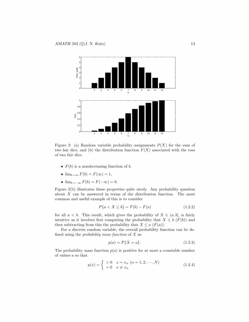
1. Let X denote the random variable which is defined as the sum of two fairdice, then the random variable is assigned the values
P{X = 2} = P{(1, 1)} = 1/36

AMATH 582 ( c©J. N. Kutz) 12
P{X = 3} = P{(1, 2), (2, 1)} = 2/36
P{X = 4} = P{(1, 3), (3, 1), (2, 2, )} = 3/36
P{X = 5} = P{(1, 4), (4, 1), (2, 3), (3, 2)} = 4/36
P{X = 6} = P{(1, 5), (5, 1), (2, 4), (4, 2), (3, 3)} = 5/36
P{X = 7} = P{(1, 6), (6, 1), (2, 5), (5, 2), (3, 4), (4, 3)} = 6/36
P{X = 8} = P{(2, 6), (6, 2), (3, 5), (5, 3), (4, 4)} = 5/36
P{X = 9} = P{(3, 6), (6, 3), (4, 5), (5, 4)} = 4/36
P{X = 10} = P{(4, 6), (6, 4), (5, 5)} = 3/36
P{X = 11} = P{(5, 6), (6, 5)} = 2/36
P{X = 12} = P{(6, 6)} = 1/36 .
Thus the random variable X can take on integer values between two andtwelve with the probability for each assigned above. Since the above eventsare all possible outcomes which are mutually exclusive, then
P(∪12n=2{X = n}
)=
12∑
n=2
P{X = n} = 1
Figure 2 illustrates the probability as a function of X as well as its distri-bution function.
2. Suppose a coin is tossed having probability p of coming up heads, untilthe first heads appears. Then define the random variable N which denotesthe number of flips required to generate the first heads. Thus
P{N = 1} = P{H} = p
P{N = 2} = P{(T,H)} = (1 − p)p
P{N = 3} = P{(T, T,H)} = (1 − p)2p
...
P{N = n} = P{(T, T, · · · , T,H)} = (1 − p)n−1p
and again the random variable takes on discrete values.
In the above examples, the random variables took on a finite, or countable,number of possible values. Such random variables are discrete random variables.The cumulative distribution function, or more simply the distribution functionF (·) of the random variable X (See Fig. 2) is defined for any real number b(−∞ < b <∞) by
F (b) = P{X ≤ b} . (1.2.1)
Thus the F (b) denotes the probability of a random variable X taking on a valuewhich is less than or equal to b. Some properties of the distribution functionare as follows:
AMATH 582 ( c©J. N. Kutz) 13
2 3 4 5 6 7 8 9 10 11 120
1
2
3
4
5
6
X
P(X
) (
x36)
2 3 4 5 6 7 8 9 10 11 120
0.2
0.4
0.6
0.8
1
X
F(X
)
Figure 2: (a) Random variable probability assignments P (X) for the sum oftwo fair dice, and (b) the distribution function F (X) associated with the tossof two fair dice.
• F (b) is a nondecreasing function of b,
• limb→∞ F (b) = F (∞) = 1,
• limb→−∞ F (b) = F (−∞) = 0.
Figure 2(b) illustrates these properties quite nicely. Any probability questionabout X can be answered in terms of the distribution function. The mostcommon and useful example of this is to consider
P{a < X ≤ b} = F (b) − F (a) (1.2.2)
for all a < b. This result, which gives the probability of X ∈ (a, b], is fairlyintuitive as it involves first computing the probability that X ≤ b (F (b)) andthen subtracting from this the probability that X ≤ a (F (a)).
For a discrete random variable, the overall probability function can be de-fined using the probability mass function of X as
p(a) = P{X = a} . (1.2.3)
The probability mass function p(a) is positive for at most a countable numberof values a so that
p(x) =
{> 0 x = xn (n = 1, 2, · · · , N)= 0 x 6= xn
(1.2.4)
AMATH 582 ( c©J. N. Kutz) 14
Further, since X must take on one of the values of xn, then
N∑
n=1
p(xn) = 1 . (1.2.5)
The cumulative distribution is defined as follows:
F (a) =∑
xn<a
p(xn) . (1.2.6)
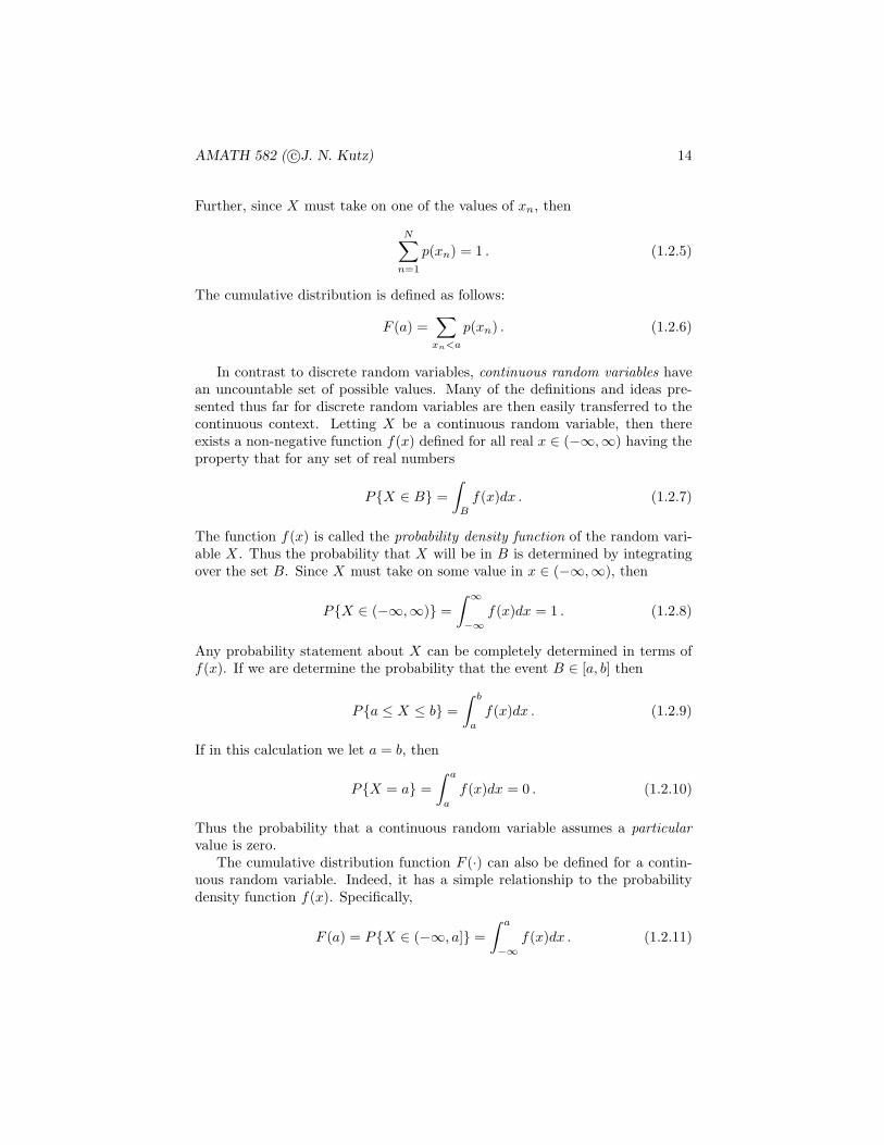
In contrast to discrete random variables, continuous random variables havean uncountable set of possible values. Many of the definitions and ideas pre-sented thus far for discrete random variables are then easily transferred to thecontinuous context. Letting X be a continuous random variable, then thereexists a non-negative function f(x) defined for all real x ∈ (−∞,∞) having theproperty that for any set of real numbers
P{X ∈ B} =
∫
B
f(x)dx . (1.2.7)
The function f(x) is called the probability density function of the random vari-able X . Thus the probability that X will be in B is determined by integratingover the set B. Since X must take on some value in x ∈ (−∞,∞), then
P{X ∈ (−∞,∞)} =
∫ ∞
−∞
f(x)dx = 1 . (1.2.8)
Any probability statement about X can be completely determined in terms off(x). If we are determine the probability that the event B ∈ [a, b] then
P{a ≤ X ≤ b} =
∫ b
a
f(x)dx . (1.2.9)
If in this calculation we let a = b, then
P{X = a} =
∫ a
a
f(x)dx = 0 . (1.2.10)
Thus the probability that a continuous random variable assumes a particularvalue is zero.
The cumulative distribution function F (·) can also be defined for a contin-uous random variable. Indeed, it has a simple relationship to the probabilitydensity function f(x). Specifically,
F (a) = P{X ∈ (−∞, a]} =
∫ a
−∞
f(x)dx . (1.2.11)

AMATH 582 ( c©J. N. Kutz) 15
Thus the density is the derivative of the cumulative distribution function. Animportant interpretation of the density function is obtained by considering thefollowing
P{a− ǫ
2≤ X ≤ a+
ǫ
2
}=
∫ a+ǫ2
a−ǫ/2
f(x)dx ≈ ǫf(a) . (1.2.12)
The sifting property of this integral illustrates that the density function f(a)measures how likely it is that the random variable will be near a.
Having established key properties and definitions concerning discrete andrandom variables, it is illustrative to consider some of the most common randomvariables used in practice. Thus consider first the following discrete randomvariables:
1. Bernoulli Random Variable: Consider a trial whose outcome can ei-ther be termed a success or failure. Let the random variable X = 1 ifthere is a success and X = 0 if there is failure, then the probability massfunction of X is given by
p(0) = P{X = 0} = 1 − p
p(1) = P{X = 1} = p
where p (0 ≤ p ≤ 1) is the probability that the trial is a success.
2. Binomial Random Variable: Suppose n independent trials are per-formed, each of which results in a success with probability p and failurewith probability 1−p. Denote X as the number of successes that occur inn such trials. Then X is is a binomial random variable with parameters(n, p) and the probability mass function is given by
p(j) =
(nj
)pj(1 − p)n−j
where
(nj
)= n!/((n − j)!j!) is the number of different groups of j
objects that can be chosen from a set of n objects. For instance, ifn = 3 and j = 2, then this binomial coefficient is 3!/(1!2!)=3 repre-senting the fact that there are three ways to have successes in three trials:(s, s, f), (s, f, s), (f, s, s).
3. Poisson Random Variable: A Poisson random variable with parameterλ is defined such that
p(n) = P{X = n} = e−λλnn!
n = 0, 1, 2, · · ·
for some λ > 0. The Poisson random variable has an enormous rangeof applications across the sciences as it represents, to some extent, theexponential distribution of many systems.

AMATH 582 ( c©J. N. Kutz) 16
In a similar fashion, a few of the more common continuous random variablescan be highlighted here:
1. Uniform Random Variable: A random variable is said to be uniformlydistributed over the interval (0, 1) if its probability density function isgiven by
f(x) =
{1, 0 < x < 10, otherwise
.
More generally, the definition can be extended to any interval (α, β) withthe density function being given by
f(x) =
{ 1β−α , α < x < β
0, otherwise.
The associated distribution function is then given by
F (a) =
0, a < αa−αβ−α , α < a < β
1, a ≥ β
2. Exponential Random Variable: Given a positive constant λ > 0, thedensity function for this random variable is given by
f(x) =
{λe−λx, x ≥ 00, x ≤ 0
This is the continuous version of the Poisson distribution considered forthe discrete case. Its distribution function is given by
F (a) =
∫ a
0
λe−λxdx = 1 − e−λa, a > 0 .
3. Normal Random Variable: Perhaps the most important of them all isthe normal random variable with parameters µ and σ2 defined by
f(x) =1√
2πσ2e−(x−µ)2/2σ2
, −∞ < x <∞, .
Although we have not defined them yet, the parameters µ and σ referto the mean and variance of this distribution respectively. Further, theGaussian shape produces the ubiquitous bell-shaped curve that is alwaystalked about in the context of large samples, or perhaps grading. Itsdistribution is given by the error function erf(a), one of the most commonfunctions for look-up tables in mathematics.
AMATH 582 ( c©J. N. Kutz) 17
Expectation, moments and variance of random variables
The expectation value of a random variable is defined as follows:
E[X ] =∑
x:p(x)>0
xp(x)
for a discrete random variable, and
E[X ] =
∫ ∞
−∞
xf(x)dx
for a continous random variable. Both of these definitions illustrate the thatthe expectation is a weighted average whose weight is the probability that Xassumes at that value. Typically, the expectation is interpreted as the averagevalue of the random variable. Some examples will serve to illustrate this point:
1. The expected value E[X ] of the roll of a fair die is given by
E[X ] = 1(1/6) + 2(1/6) + 3(1/6) + 4(1/6) + 5(1/6) + 6(1/6) = 7/2
2. The expectation E[X ] of a Bernoulli variable is
E[X ] = 0(1 − p) + 1(p) = p
showing that the expected number of successes in a single trial is just theprobability that the trial will be a success.
3. The expectation E[X ] of a binomial or Poisson random variable is
E[X ] = np binomial
E[X ] = λ Poisson
4. The expectation of a continuous uniform random variable is
E[X ] =
∫ β
α
x
β − αdx =
α+ β
2
5. The expectation E[X ] of an exponential or normal random variable is
E[X ] = 1/λ exponential
E[X ] = µ normal
The idea of expectation can be generalized beyond the standard expectationE[X ]. Indeed, we can consider the expectation of any function of the random

AMATH 582 ( c©J. N. Kutz) 18
variable X . Thus to compute the expectation of some function g(X), the dis-crete and continuous expectations become:
E[g(X)] =∑
x:p(x)>0
g(x)p(x) (1.2.13a)
E[g(X)] =
∫ ∞
−∞
g(x)f(x)dx (1.2.13b)
This also then leads us to the idea of higher-moments of a random variable, i.e.g(X) = Xn so that
E[Xn] =∑
x:p(x)>0
xnp(x) (1.2.14a)
E[Xn] =
∫ ∞
−∞
xnf(x)dx . (1.2.14b)
The first moment is essentially the mean, the second moment will be related tothe variance, the third and fourth moments measure the skewness (asymmetryof the probability distribution) and the kurtosis (the flatness or sharpness) ofthe distribution.
Now that these probability ideas are in place, the quantifies of greatest andmost practical interest can be considered, namely the ideas of mean and variance(and standard deviation, which is defined as the square root of the variance).The mean has already been defined, while the variance of a random variable isgiven by
V ar[X ] = E[(X − E[X ])2] = E[X2] − E[X ]2 (1.2.15)
The second form can be easily manipulated from the first. Note that dependingupon your scientific community of origin E[X ] = x =< x >. It should benoted that the normal distribution has V ar(X) = σ2, standard deviation σ,and skewness of zero.
Joint probability distribution and covariance
The mathematical framework is now in place to discuss what is perhaps, forthis course, the most important use of our probability and statistical thinking,namely the relation between two or more random variables. Ultimately, this as-sesses whether or not two variables depend upon each other. A joint cumulativeprobability distribution function of two random variables X and Y is given by
F (a, b) = P{X ≤ a, Y ≤ b}, −∞ < a, b <∞ . (1.2.16)
The distribution of X or Y can be obtained by considering
FX(a) = P{X ≤ a} = P{X ≤ a, Y ≤ ∞} = F (a,∞) (1.2.17a)
FY (b) = P{Y ≤ b} = P{Y ≤ b,X ≤ ∞} = F (∞, b) . (1.2.17b)

AMATH 582 ( c©J. N. Kutz) 19
The random variables X and Y are jointly continuous if there exists a functionf(x, y) defined for real x and y so that for any set of real numbers A and B
P{X ∈ A, Y ∈ B} =
∫
A
∫
B
f(x, y)dxdy . (1.2.18)
The function f(x, y) is called the joint probability density function of X and Y .The probability density of X or Y can be extracted from f(x, y) as follows:
P{X∈A}=P{X∈A, Y ∈(−∞,∞)}=
∫ ∞
−∞
∫
A
f(x, y)dxdy=
∫
A
fX(x)dx
(1.2.19)where fX(x) =
∫ ∞
−∞ f(x, y)dy. Similarly, the probability density function of Y
is fY (y) =∫ ∞
−∞f(x, y)dx. As previously, to determine a function of the random
variables X and Y , then
E[g(X,Y )] =
{ ∑y
∑x g(x, y)p(x, y) discrete
∫ ∞
−∞
∫ ∞
−∞g(x, y)f(x, y)dxdy continuous
(1.2.20)
Jointly distributed variables lead naturally to a discussion of whether thevariables are independent. Two random variables are said to be independent if
P{X ≤ a, Y ≤ b} = P{X ≤ a}P{Y ≤ b} (1.2.21)
In terms of the joint distribution function F of X and Y , independence isestablished if F (a, b) = FX(a)FY (b) for all a, b. The independence assumptionessentially reduces to the following:
f(x, y) = fX(x)fY (y) . (1.2.22)
This further implies
E[g(X)h(Y )] = E[g(X)]E[h(Y )] . (1.2.23)
Mathematically, the case of independence allows for essentially a separation ofthe random variables X and Y .
What is, to our current purposes, more interesting is the idea of depen-dent random variables. For such variables, the concept of covariance can beintroduced. This is defined as
Cov(X,Y ) = E[(X − E[X ])(Y − E[Y ])] = E[XY ] − E[X ]E[Y ] . (1.2.24)
If two variables are independent then Cov(X,Y) = 0. Alternatively, as theCov(X,Y) approaches unity, it implies that X and Y are essentially directly,or strongly, correlated random variables. This will serve as a basic measure ofthe statistical dependence of our data sets. It should be noted that althoughtwo independent variables implies Cov(X,Y)= 0, the converse is not necessarytrue, i.e. Cov(X,Y)=0 does not imply independence of X and Y .
AMATH 582 ( c©J. N. Kutz) 20
MATLAB commands
The following are some of the basic commands in MATLAB that we will use forcomputing the above mentioned probability and statistical concepts.
1. rand(m,n): This command generates anm×nmatrix of random numbersfrom the uniform distribution on the unit interval.
2. randn(m,n): This command generates an m × n matrix of normallydistributed random numbers with zero mean and unit variance.
3. mean(X): This command returns the mean or average value of each col-umn of the matrix X.
4. var(X): This computes the variance of each row of the matrix X. To pro-duce and unbiased estimator, the variance of the population is normalizedby N − 1 where N is the sample size.
5. std(X): This computes the standard deviation of each row of the matrixX. To produce and unbiased estimator, the standard deviation of thepopulation is normalized by N − 1 where N is the sample size.
6. cov(X): If X is a vector, it returns the variance. For matrices, where eachrow is an observation, and each column a variable, the command returnsa covariance matrix. Along the diagonal of this matrix is the variance ofeach column.
1.3 Hypothesis testing and statistical significance
With the key concepts of probability theory in hand, statistical testing of datacan now be pursued. But before doing so, a few key results concerning a largenumber of random variables or large number of trials should be explicitly stated.
Limit theorems
Two theorems of probability theory are important to establish before discussingtesting of hypothesis via statistics: they are the strong law of large numbers andthe central limit theorem. They are, perhaps, the most well-known and mostimportant practical results in probability theory.
Theorem: Strong law of large numbers: Let X1, X2, · · · be a sequence of inde-pendent random variables having a common distribution, and let E[Xj ] = µ.Then, with probability one,
X1 +X2 + · · · +Xn
n→ µ as n→ ∞ (1.3.1)

AMATH 582 ( c©J. N. Kutz) 21
As an example of the strong law of large numbers, suppose that a sequenceof independent trials are performed. Let E be a fixed event and denote by P (E)the probability that E occurs on any particular trial. Letting
Xj =
{1, if E occurs on the jth trial0, if E does not occur on the jth trial
(1.3.2)
The theorem states that with probability one
X1 +X2 + · · · +Xn
n→ E[X ] = P (E) . (1.3.3)
Since X1+X2+ · · ·+Xn represents the number of times that the event E occursin n trials, this result can be interpreted as the fact that, with probability one,the limiting proportion of time that the event E occurs is just P (E).
Theorem: Central Limit Theorem: Let X1, X2, · · · be a sequence of indepen-dent random variables each with mean µ and variance σ2. Then the distributionof the quantity
X1 +X2 + · · · +Xn − nµ
σ√n
(1.3.4)
tends to the standard normal distribution as n→ ∞ so that
P
{X1 +X2 + · · · +Xn − nµ
σ√n
≤ a
}→ 1√
2π
∫ a
−∞
e−x2/2dx (1.3.5)
as n→ ∞. The most important part of this result: it holds for any distributionof Xj . Thus for a large enough sampling of data, i.e. a sequence of independentrandom variables that goes to infinity, one should observe the ubiquitous bell-shaped probability curve of the normal distribution. This is a powerful resultindeed, provided you have a large enough sampling. And herein lies both itspower, and susceptibility to overstating results. The fact is, the normal distri-bution has some very beautiful mathematical properties, leading us to considerthis central limit almost exclusively when testing for statistical significance.
As an example, consider a binomially distributed random variable X withparameters n (n is the number of events) and p (p is the probability of a successof an event). The distribution of
X − E[X ]√V ar[X ]
=X − np√np(1 − p)
(1.3.6)
approaches the standard normal distribution as n → ∞. Empirically, it hasbeen found that the normal approximation will, in general, be quite good forvalues of n satisfying np(1 − p) ≥ 10.

AMATH 582 ( c©J. N. Kutz) 22
Statistical decisions
In practice, the power of probability and statistics comes into play in makingdecisions, or drawing conclusions, based upon a limited sampling or informationinformation of an entire population (of data). Indeed, it is often impossible orimpractical to examine the entire population. Thus a sample of the populationis considered instead. This is called the sample. The goal is to infer facts ortrends about the entire population with this limited sample size. The process ofobtaining samples is called sampling, while process of drawing conclusions aboutthis sample is called statistical inference. Using these ideas to make decisionsabout a population based upon the sample information is termed statisticaldecisions.
In general, these definitions are quite intuitive and also quite well knownto us. Statistical inference, for instance, is used extensively in polling data forelections. In such a scenario, county, state, and national election projectionsare made well before the election based upon sampling a small portion of thepopulation. Statistical decision making on the other hand is used extensivelyto determine whether a new medical treatment or drug is, in fact, effective incuring a disease or ailment.
In what follows, the focus will be upon statistical decision making. In at-tempting to reach a decision, it is useful to make assumptions or guesses aboutthe population involved. Much like an analysis proof, you can reach a conclusionby assuming something is true and proving it to be so, or assuming the oppositeis true and proving that it is false, for instance, by a counter example. Thereis no difference with statistical decision making. In this case, all the statisti-cal tests are hypothesis driven. Thus a statistical hypothesis is proposed andits validity investigated. As with analysis, some hypothesis are explicitly con-structed for the purpose of rejection, or nullifying the hypothesis. For example,to decide whether a coin is fair or loaded, the hypothesis is formulated that thecoin is fair with p = 0.5 as the probability of heads. To decide if one procedureis better or worse than another, the hypothesis formulated is that there is nodifference between the procedures. Such hypotheses are called null hypothesisand denoted by H0. Any hypothesis which differs from a given hypothesis iscalled an alternative hypothesis and is denoted by H1.
Tests for statistical significance
The ultimate goal in statistical decision making is to develop tests that are ca-pable of allowing us to accept or reject a hypothesis with a certain, quantifiableconfidence level. Procedures that allow us to do this are called tests of hypoth-esis, tests of significance or rules of decision. Overall, they fall within the aegisof the ideas of statistical significance.
In making such statistical decisions, there is some probability that erroneousconclusion will be reached. Such errors are classified as follows:

AMATH 582 ( c©J. N. Kutz) 23
• Type I error: If a hypothesis is rejected when it should be accepted.
• Type II error: If a hypothesis is accepted when it should be rejected.
As an example, suppose a fair coin (p = 0.5 for achieving heads or tails) istossed 100 times and unbelievably, 100 heads in a row results. Any statisticaltest based upon assuming that the coin is fair is going to be rejected and aType I error will occur. If on the other hand, a loaded coin twice as likely toproduce a heads than a tails (p = 2/3 for achieving a heads and 1− p = 1/3 forproducing a tails) is tossed 100 times and heads and tails both appear 50 times,then a hypothesis about a biased coin will be rejected and a Type II error willbe made.
What is important in making the statistical decision is the level of signif-icance of the test. This probability is often denoted by α, and in practice itis often taken to be 0.05 or 0.01. These correspond to a 5% or 1% level ofsignificance, or alternatively, we are 95% or 99% confident respectively that ourdecision is correct. Basically, in these tests, we will be wrong 5% or 1% of thetime.
Hypothesis testing with the normal distribution
For large samples, the central limit theorem asserts that the statistics has a nor-mal distribution (or nearly so) with mean µs and standard deviation σs. Thusmany statistical decision tests are specifically geared to the normal distribution.Consider the normal distribution with mean µ and variance σ2 such that thedensity is given by
f(x) =1√
2πσ2e−(x−µ)2/2σ2 −∞ < x <∞ (1.3.7)
and where the cumulative distribution is given by
F (x) = P (X ≤ x) =1√
2πσ2
∫ x
−∞
e−(x−µ)2/2σ2
dx . (1.3.8)
With the change of variable
Z =X − µ
σ(1.3.9)
the standard normal density function is given by
f(z) =1√2πe−x
2/2 (1.3.10)
with the corresponding distribution function (related to the error function)
F (z) =1√2π
∫ z
−∞
e−u2/2du =
1
2
[1 + erf
(z√2
)]. (1.3.11)
AMATH 582 ( c©J. N. Kutz) 24
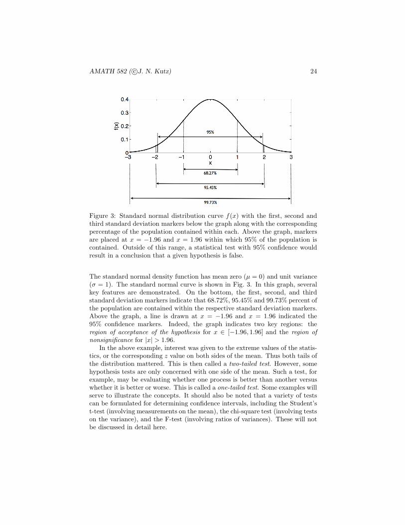
Figure 3: Standard normal distribution curve f(x) with the first, second andthird standard deviation markers below the graph along with the correspondingpercentage of the population contained within each. Above the graph, markersare placed at x = −1.96 and x = 1.96 within which 95% of the population iscontained. Outside of this range, a statistical test with 95% confidence wouldresult in a conclusion that a given hypothesis is false.
The standard normal density function has mean zero (µ = 0) and unit variance(σ = 1). The standard normal curve is shown in Fig. 3. In this graph, severalkey features are demonstrated. On the bottom, the first, second, and thirdstandard deviation markers indicate that 68.72%, 95.45% and 99.73% percent ofthe population are contained within the respective standard deviation markers.Above the graph, a line is drawn at x = −1.96 and x = 1.96 indicated the95% confidence markers. Indeed, the graph indicates two key regions: theregion of acceptance of the hypothesis for x ∈ [−1.96, 1.96] and the region ofnonsignificance for |x| > 1.96.
In the above example, interest was given to the extreme values of the statis-tics, or the corresponding z value on both sides of the mean. Thus both tails ofthe distribution mattered. This is then called a two-tailed test. However, somehypothesis tests are only concerned with one side of the mean. Such a test, forexample, may be evaluating whether one process is better than another versuswhether it is better or worse. This is called a one-tailed test. Some examples willserve to illustrate the concepts. It should also be noted that a variety of testscan be formulated for determining confidence intervals, including the Student’st-test (involving measurements on the mean), the chi-square test (involving testson the variance), and the F-test (involving ratios of variances). These will notbe discussed in detail here.
AMATH 582 ( c©J. N. Kutz) 25
Example: A fair coin. Design a decision rule to test the null hypothesis H0
that a coin is fair if a sample of 64 tosses of the coin is taken and if the level ofsignificance is 0.05 or 0.01.
The coin toss is an example of a binomial distribution as a success (heads)and failure (tails). Under the null hypothesis that the coin is fair (p = 0.5 forachieving either heads or tails) the binomial mean and standard deviation canbe easily calculated for n events:
µ = np = 64 × 0.5 = 32
σ =√np(1 − p) =
√64 × 0.5 × 0.5 = 4 .
The statistical decision must now be formulated in terms of the standard normalvariable Z where
Z =X − µ
σ=X − 32
4.
For the hypothesis to hold with 95% confidence (or 99% confidence), then z ∈[−1.96, 1.96]. Thus the following must be satisfied:
−1.96 ≤ X − 32
4≤ 1.96 → 24.16 ≤ X ≤ 39.84
Thus if in a trial of 64 flips heads appears between 25 and 39 times inclusive,the hypothesis is true with 95% confidence. For 99% confidence, heads mustappear between 22 and 42 times inclusive.
Example: Class scores. An examination was given to two classes of 40 and 50students respectively. In the first class, the mean grade was 74 with a standarddeviation of 8, while in the second class the mean was 78 with standard devia-tion 7. Is there a statistically significant difference between the performance ofthe two classes at a level of significance of 0.05?
Consider that the two classes come from two populations having respectivemeans µ1 and µ2. Then the following null hypothesis and alternative hypothesiscan be formulated.
H0 : µ1 = µ2, and the difference is merely due to chance
H1 : µ1 6= µ2, and there is a significant difference between classes
Under the null hypothesis H0, both classes come from the same population.The mean and standard deviation of the differences of these is given by
µX1−X2= 0
σX1−X2=
√σ2
1
n1+σ2
2
n2=
√82
40+
72
50= 1.606
AMATH 582 ( c©J. N. Kutz) 26
where the standard deviations have been used as estimates for σ1 and σ2. Theproblem is thus formulated in terms of a new variable representing the differenceof the means
Z =X1 − X2
σX1−X2
=74 − 78
1.606= −2.49
(a) For a two-tailed test, the results are significant if |Z| > 1.96. Thus it mustbe concluded that there is a significant difference in performance to the twoclasses with the second class probably being better(b) For the same test with 0.01 significance, then the results are significant for|Z| > 2.58 so that at a 0.01 significance level there is no statistical differencebetween the classes.
Example: Rope breaking (Student’s t-distribution). A test of strengthof 6 ropes manufactured by a company showed a breaking strength of 7750lband a standard deviation of 145lb, whereas the manufacturer claimed a meanbreaking strength of 8000lb. Can the manufacturers claim be supported at asignificance level of 0.05 or 0.01?
The decision is between the hypotheses
H0 : µ = 8000lb, the manufacturer is justified
H1 : µ < 8000lb, the manufacturer’s claim is unjustified
where a one-tailed test is to be considered. Under the null hypothesis H0 andthe small sample size, the Student’s t-test can be used so that
T =X − µ
S
√n− 1 =
7750 − 8000
145
√6 − 1 = −3.86
As n → ∞, the Student’s t-distribution goes to the normal distribution. Butin this case of a small sample, the degree of freedom is of this distribution is6-1=5 and a 0.05 (0.01) significance is achieved with T > −2.01 (or T > −3.36).In either case, with T = −3.86 it is extremely unlikely that the manufacture’sclaim is justified.
2 Time-Frequency Analysis: Fourier Transformsand Wavelets
Fourier transforms, and more generally, spectral transforms, are one of the mostpowerful and efficient techniques for solving a wide variety of problems arisingthe physical, biological and engineering sciences. The key idea of the Fouriertransform, for instance, is to represent functions and their derivatives as sums ofcosines and sines. This operation can be done with the Fast-Fourier transform

AMATH 582 ( c©J. N. Kutz) 27
(FFT) which is an O(N logN) operation. Thus the FFT is faster than mostlinear solvers of O(N2). The basic properties and implementation of the FFTwill be considered here along with other time-frequency analysis techniques,including wavelets.
2.1 Basics of Fourier Series and the Fourier Transform
Fourier introduced the concept of representing a given function by a trigono-metric series of sines and cosines:
f(x) =a0
2+
∞∑
n=1
(an cosnx+ bn sinnx) x ∈ (−π, π] . (2.1.1)
At the time, this was a rather startling assertion, especially as the claim heldeven if the function f(x), for instance, was discontinuous. Indeed, when workingwith such series solutions, many questions arise concerning the convergence ofthe series itself. Another, of course, concerns the determination of the expansioncoefficients an and bn. Assume for the moment that Eq. (2.1.1) is a uniformlyconvergent series, then multiplying by cosmx gives the following uniformly con-vergent series
f(x) cosmx =a0
2cosmx+
∞∑
n=1
(an cosnx cosmx+ bn sinnx cosmx) . (2.1.2)
Integrating both sides from x ∈ [−π, π] yields the following∫ π
−π
f(x) cosmxdx =a0
2
∫ π
−π
cosmxdx
+
∞∑
n=1
(an
∫ π
−π
cosnx cosmxdx + bn
∫ π
−π
sinnx cosmxdx
). (2.1.3)
But the sine and cosine expressions above are subject to the following orthogo-nality properties.
∫ π
−π
sinnx cosmxdx = 0 ∀ n,m (2.1.4a)
∫ π
−π
cosnx cosmxdx =
{0 n 6= mπ n = m
(2.1.4b)
∫ π
−π
sinnx sinmxdx = 0
{0 n 6= mπ n = m
. (2.1.4c)
Thus we find the following formulas for the coefficients an and bn
an =1
π
∫ π
−π
f(x) cosnxdx n ≥ 0 (2.1.5a)
bn =1
π
∫ π
−π
f(x) sinnxdx n > 0 (2.1.5b)

AMATH 582 ( c©J. N. Kutz) 28
which are called the Fourier coefficients.The expansion (2.1.1) must, by construction, produce 2π-periodic functions
since they are constructed form sines and cosines on the interval x ∈ (−π, π]. Inaddition to these 2π-periodic solutions, one can consider expanding a functionf(x) defined on x ∈ (0, π] as an even periodic function on x ∈ (−π, π] byemploying only the cosine portion of the expansion (2.1.1) or as an odd periodicfunction on x ∈ (−π, π] by employing only the sine portion of the expansion(2.1.1).
Using these basic ideas, the complex version of the expansion produces theFourier series on the domain x ∈ [−L,L] is given by
f(x) =
∞∑
−∞
cneinπx/L x ∈ [−L,L] (2.1.6)
with the corresponding Fourier coefficients
cn =1
2L
∫ L
−L
f(x)e−inπx/Ldx . (2.1.7)
Although the Fourier series is now complex, the function f(x) is still assumedto be real. Thus the following observations are of note: (i) c0 is real andc−n = cn∗, (ii) if f(x) is even, all cn are real, and (iii) if f(x) is odd, c0 = 0and all cn are purely imaginary. These results follow from Euler’s identity:exp(±ix) = cosx ± i sinx. The convergence properties of this representationwill not be considered here except that it will be noted that at discontinuity off(x), the Fourier series converges to the mean of the left and right value of thediscontinuity.
The Fourier Transform
The Fourier Transform is an integral transform defined over the entire linex ∈ [−∞,∞]. The Fourier transform and its inverse are defined as
F (k) =1√2π
∫ ∞
−∞
e−ikxf(x)dx (2.1.8a)
f(x) =1√2π
∫ ∞
−∞
eikxF (k)dk . (2.1.8b)
There are other equivalent definitions. However, this definition will serve toillustrate the power and functionality of the Fourier transform method. Weagain note that formally, the transform is over the entire real line x ∈ [−∞,∞]whereas our computational domain is only over a finite domain x ∈ [−L,L].Further, the Kernel of the transform, exp(±ikx), describes oscillatory behavior.Thus the Fourier transform is essentially an eigenfunction expansion over allcontinuous wavenumbers k. And once we are on a finite domain x ∈ [−L,L],the continuous eigenfunction expansion becomes a discrete sum of eigenfunctionsand associated wavenumbers (eigenvalues).
AMATH 582 ( c©J. N. Kutz) 29
Derivative Relations
The critical property in the usage of Fourier transforms concerns derivativerelations. To see how these properties are generated, we begin by consideringthe Fourier transform of f ′(x). We denote the Fourier transform of f(x) as
f(x). Thus we find
f ′(x) =1√2π
∫ ∞
−∞
e−ikxf ′(x)dx = f(x)e−ikx|∞−∞ +ik√2π
∫ ∞
−∞
e−ikxf(x)dx .
(2.1.9)Assuming that f(x) → 0 as x→ ±∞ results in
f ′(x) =ik√2π
∫ ∞
−∞
e−ikxf(x)dx = ikf(x) . (2.1.10)
Thus the basic relation f ′ = ikf is established. It is easy to generalize thisargument to an arbitrary number of derivatives. The final result is the followingrelation between Fourier transforms of the derivative and the Fourier transformitself
f (n) = (ik)nf . (2.1.11)
This property is what makes Fourier transforms so useful and practical.As an example of the Fourier transform, consider the following differential
equationy′′ − ω2y = −f(x) x ∈ [−∞,∞] . (2.1.12)
We can solve this by applying the Fourier transform to both sides. This givesthe following reduction
y′′ − ω2y = −f−k2y − ω2y = −f(k2 + ω2)y = f
y =f
k2 + ω2. (2.1.13)
To find the solution y(x), we invert the last expression above to yield
y(x) =1√2π
∫ ∞
−∞
eikxf
k2 + ω2dk . (2.1.14)
This gives the solution in terms of an integral which can be evaluated analyti-cally or numerically.

AMATH 582 ( c©J. N. Kutz) 30
The Fast Fourier Transform
The Fast Fourier transform routine was developed specifically to perform theforward and backward Fourier transforms. In the mid 1960s, Cooley and Tukeydeveloped what is now commonly known as the FFT algorithm [3]. Their al-gorithm was named one of the top ten algorithms of the 20th century for onereason: the operation count for solving a system dropped to O(N logN). ForN large, this operation count grows almost linearly like N . Thus it represents agreat leap forward from Gaussian elimination and LU decomposition. The keyfeatures of the FFT routine are as follows:
1. It has a low operation count: O(N logN).
2. It finds the transform on an interval x ∈ [−L,L]. Since the integrationKernel exp(ikx) is oscillatory, it implies that the solutions on this finiteinterval have periodic boundary conditions.
3. The key to lowering the operation count to O(N logN) is in discretizingthe range x ∈ [−L,L] into 2n points, i.e. the number of points should be2, 4, 8, 16, 32, 64, 128, 256, · · ·.
4. The FFT has excellent accuracy properties, typically well beyond that ofstandard discretization schemes.
We will consider the underlying FFT algorithm in detail at a later time. Formore information at the present, see [3] for a broader overview.
The practical implementation of the mathematical tools available in MAT-LAB is crucial. This lecture will focus on the use of some of the more sophis-ticated routines in MATLAB which are cornerstones to scientific computing.Included in this section will be a discussion of the Fast Fourier Transform rou-tines (fft, ifft, fftshift, ifftshift, fft2, ifft2), sparse matrix construction (spdiag,spy), and high end iterative techniques for solving Ax = b (bicgstab, gmres).These routines should be studied carefully since they are the building blocks ofany serious scientific computing code.
Fast Fourier Transform: FFT, IFFT, FFTSHIFT, IFFTSHIFT2
The Fast Fourier Transform will be the first subject discussed. Its implemen-tation is straightforward. Given a function which has been discretized with 2n
points and represented by a vector x, the FFT is found with the commandfft(x). Aside from transforming the function, the algorithm associated with theFFT does three major things: it shifts the data so that x ∈ [0, L] → [−L, 0]and x ∈ [−L, 0] → [0, L], additionally it multiplies every other mode by −1, andit assumes you are working on a 2π periodic domain. These properties are aconsequence of the FFT algorithm discussed in detail at a later time.
AMATH 582 ( c©J. N. Kutz) 31
To see the practical implications of the FFT, we consider the transform ofa Gaussian function. The transform can be calculated analytically so that wehave the exact relations:
f(x) = exp(−αx2) → f(k) =1√2α
exp
(− k2
4α
). (2.1.15)
A simple MATLAB code to verify this with α = 1 is as follows
clear all; close all; % clear all variables and figures
L=20; % define the computational domain [-L/2,L/2]
n=128; % define the number of Fourier modes 2^n
x2=linspace(-L/2,L/2,n+1); % define the domain discretization
x=x2(1:n); % consider only the first n points: periodicity
u=exp(-x.*x); % function to take a derivative of
ut=fft(u); % FFT the function
utshift=fftshift(ut); % shift FFT
figure(1), plot(x,u) % plot initial gaussian
figure(2), plot(abs(ut)) % plot unshifted transform
figure(3), plot(abs(utshift)) % plot shifted transform
The second figure generated by this script shows how the pulse is shifted. Byusing the command fftshift, we can shift the transformed function back to itsmathematically correct positions as shown in the third figure generated. How-ever, before inverting the transformation, it is crucial that the transform isshifted back to the form of the second figure. The command ifftshift does this.In general, unless you need to plot the spectrum, it is better not to deal withthe fftshift and ifftshift commands. A graphical representation of the fft pro-cedure and its shifting properties is illustrated in Fig. 4 where a Gaussian istransformed and shifted by the fft routine.
FFT versus Finite-Difference Differentiation
Taylor series methods for generating approximations to derivatives of a givenfunction can also be used. In the Taylor series method, the approximationsare local since they are given by nearest neighbor coupling formulas of finitedifferences. Using the FFT, the approximation to the derivative is global sinceit uses an expansion basis of cosines and sines which extend over the entiredomain of the given function.
The calculation of the derivative using the FFT is performed trivially fromthe derivative relation formula (2.1.11). As an example of how to implement
AMATH 582 ( c©J. N. Kutz) 32
-60 -40 -20 0 20 40 60Fourier modes
-20
-10
0
10
20
real
[ffts
hift(
U)]
-10 -5 0 5 10x
0
0.2
0.4
0.6
0.8
1
u=ex
p(-x
2 )
-64 -32 0 32 64Fourier modes
0
5
10
15
abs(
fftsh
ift(U
))
-64 -32 0 32 64Fourier modes
-15
-10
-5
0
5
10
15
real
[U]
Figure 4: Fast Fourier Transform U = fft(u) of Gaussian data illustrating theshifting properties of the FFT routine. Note that the fftshift command restoresthe transform to its mathematically correct, unshifted state.
this differentiation formula, consider a specific function:
u(x) = sech(x) (2.1.16)
which has the following derivative relations
du
dx= −sech(x)tanh(x) (2.1.17a)
d2u
dx2= sech(x) − 2 sech3(x) . (2.1.17b)
A comparison can be made between the differentiation accuracy of finite dif-ference formulas of Tables ??-?? and the spectral method using FFTs. Thefollowing code generates the derivative using the FFT method along with thefinite difference O(∆x2) and O(∆x4) approximations considered with finite dif-ferences.
clear all; close all; % clear all variables and figures
AMATH 582 ( c©J. N. Kutz) 33
L=20; % define the computational domain [-L/2,L/2]
n=128; % define the number of Fourier modes 2^n
x2=linspace(-L/2,L/2,n+1); % define the domain discretization
x=x2(1:n); % consider only the first n points: periodicity
dx=x(2)-x(1); % dx value needed for finite difference
u=sech(x); % function to take a derivative of
ut=fft(u); % FFT the function
k=(2*pi/L)*[0:(n/2-1) (-n/2):-1]; % k rescaled to 2pi domain
% FFT calculation of derivatives
ut1=i*k.*ut; % first derivative
ut2=-k.*k.*ut; % second derivative
u1=real(ifft(ut1)); u2=real(ifft(ut2)); % inverse transform
u1exact=-sech(x).*tanh(x); % analytic first derivative
u2exact=sech(x)-2*sech(x).^3; % analytic second derivative
% Finite difference calculation of first derivative
% 2nd-order accurate
ux(1)=(-3*u(1)+4*u(2)-u(3))/(2*dx);
for j=2:n-1
ux(j)=(u(j+1)-u(j-1))/(2*dx);
end
ux(n)=(3*u(n)-4*u(n-1)+u(n-2))/(2*dx);
% 4th-order accurate
ux2(1)=(-3*u(1)+4*u(2)-u(3))/(2*dx);
ux2(2)=(-3*u(2)+4*u(3)-u(4))/(2*dx);
for j=3:n-2
ux2(j)=(-u(j+2)+8*u(j+1)-8*u(j-1)+u(j-2))/(12*dx);
end
ux2(n-1)=(3*u(n-1)-4*u(n-2)+u(n-3))/(2*dx);
ux2(n)=(3*u(n)-4*u(n-1)+u(n-2))/(2*dx);
figure(1)
plot(x,u,’r’,x,u1,’g’,x,u1exact,’go’,x,u2,’b’,x,u2exact,’bo’)
figure(2)
subplot(3,1,1), plot(x,u1exact,’ks-’,x,u1,’k’,x,ux,’ko’,x,ux2,’k*’)
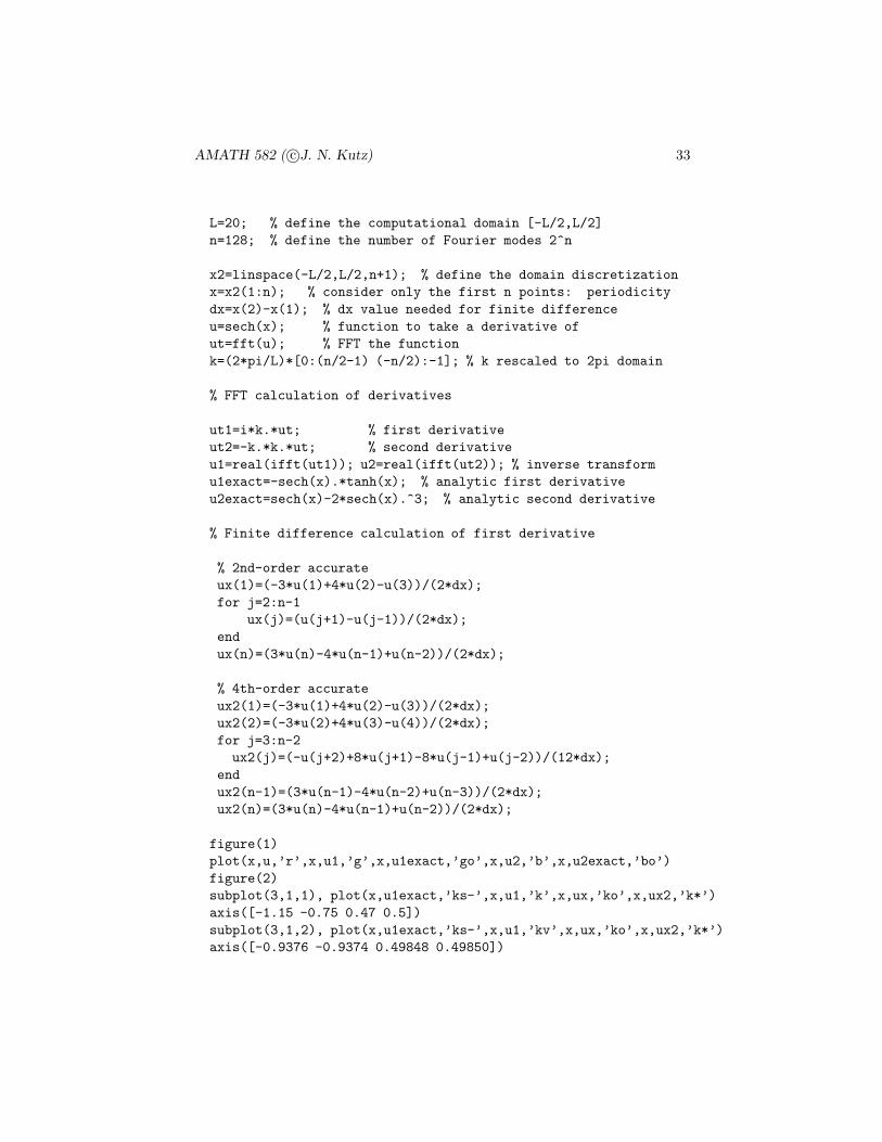
axis([-1.15 -0.75 0.47 0.5])
subplot(3,1,2), plot(x,u1exact,’ks-’,x,u1,’kv’,x,ux,’ko’,x,ux2,’k*’)
axis([-0.9376 -0.9374 0.49848 0.49850])
AMATH 582 ( c©J. N. Kutz) 34
−1.1 −1.05 −1 −0.95 −0.9 −0.85 −0.8 −0.750.47
0.48
0.49
0.5
−0.9376 −0.9375 −0.9375 −0.9374 −0.93740.4985
0.4985
0.4985
−0.9376 −0.9375 −0.9375 −0.9374 −0.9374
0.4985
0.4985
x
Figure 5: Accuracy comparison between second- and fourth-order finite differ-ence methods and the spectral FFT method for calculating the first derivative.Note that by using the axis command, the exact solution (line) and its approx-imations can be magnified near an arbitrary point of interest. Here, the topfigure shows that the second-order finite difference (circles) method is withinO(10−2) of the exact derivative. The fourth-order finite difference (star) iswithin O(10−5) of the exact derivative. Finally, the FFT method is withinO(10−6) of the exact derivative. This demonstrates the spectral accuracy prop-erty of the FFT algorithm.
subplot(3,1,3), plot(x,u1exact,’ks-’,x,u1,’kv’,x,ux,’ko’,x,ux2,’k*’)
axis([-0.9376 -0.9374 0.498487 0.498488])
Note that the real part is taken after inverse Fourier transforming due to thenumerical round off which generates a small O(10−15) imaginary part.
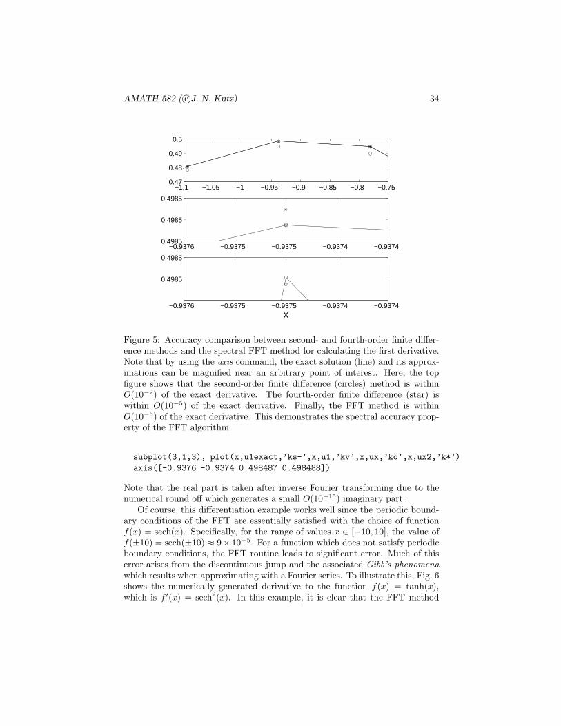
Of course, this differentiation example works well since the periodic bound-ary conditions of the FFT are essentially satisfied with the choice of functionf(x) = sech(x). Specifically, for the range of values x ∈ [−10, 10], the value off(±10) = sech(±10) ≈ 9× 10⁻⁵. For a function which does not satisfy periodicboundary conditions, the FFT routine leads to significant error. Much of thiserror arises from the discontinuous jump and the associated Gibb’s phenomenawhich results when approximating with a Fourier series. To illustrate this, Fig. 6shows the numerically generated derivative to the function f(x) = tanh(x),which is f ′(x) = sech2(x). In this example, it is clear that the FFT method
AMATH 582 ( c©J. N. Kutz) 35
−10 −5 0 5 10−1.5
−1
−0.5
0
0.5
1
1.5
x
f
df/dx
Figure 6: Accuracy comparison between the fourth-order finite differencemethod and the spectral FFT method for calculating the first derivative off(x) = tanh(x). The fourth-order finite difference (circle) is within O(10−5)of the exact derivative. In contrast, the FFT approximation (line) oscillatesstrongly and provides a highly inaccurate calculation of the derivative due tothe non-periodic boundary conditions of the given function.
is highly undesirable, whereas the finite difference method performs as well asbefore.
Higher dimensional Fourier transforms
For transforming in higher dimensions, a couple of choices in MATLAB arepossible. For 2D transformations, it is recommended to use the commandsfft2 and ifft2. These will transform a matrix A, which represents data in thex and y direction respectively, along the rows and then columns. For higherdimensions, the fft command can be modified to fft(x,[],N) where N is thenumber of dimensions. Alternatively, use fftn(x) for multi-dimensional FFTs.
2.2 FFT Application: Radar Detection and Filtering
FFTs and other related frequency transforms have revolutionized the field ofdigital signal processing and imaging. The key concept in any of these applica-tions is to use the FFT to analyze and manipulate data in the frequency domain.

AMATH 582 ( c©J. N. Kutz) 36
reflected E&M waves
sender/receiver
target
outgoing E&M waves
Figure 7: Schematic of the operation of a radar detection system. The radaremits an electromagnetic (E&M) field at a specific frequency. The radar thenreceives the reflection of this field from objects in the environment and attemptsto determine what the objects are.
There are other methods of treating the signal in the time and frequency do-main, but the simplest to begin with is the Fourier transform.
The Fourier transform is also used in quantum mechanics to represent aquantum wavepacket in either the spatial domain or the momentum (spectral)domain. Quantum mechanics is specifically mentioned due to the well-knownHeisenberg Uncertainty Principle. Simply stated, you cannot know the exactposition or momentum of a quantum particle simultaneously. This is simply aproperty of the Fourier transform itself. Essentially, a narrow signal in the timedomain corresponds to a broadband source, whereas a highly confined spectralsignature corresponds to a broad time domain source. This has significantimplication for many techniques for signal analysis. In particular, an excellentdecomposition of a given signal into its frequency components can render noinformation about when in time the different portions of signal actually occurred.Thus there is often a competition between trying to localize both in time andfrequency a signal or stream of data. Time-frequency analysis is ultimately allabout trying to resolve by the time and frequency domain in an efficient andtractable manner. Various aspects of this time-frequency processing will beconsidered in later lectures, including wavelet based methods of time-frequencyanalysis.
At this point, we discuss a very basic concept and manipulation procedure tobe performed in the frequency domain: noise attenuation via frequency (band-pass) filtering. This filtering process is fairly common in electronics and signaldetection. As a specific application or motivation for spectral analysis, considerthe process of radar detection depicted in Fig. 7. An outgoing electromagneticfield is emitted from a source which then attempts to detect the reflections ofthe emitted signal. In addition to reflections coming from the desired target,reflections can also come from geographical objects (mountains, trees, etc.) andatmospheric phenomena (clouds, precipitation, etc.). Further, there may be

AMATH 582 ( c©J. N. Kutz) 37
other sources of the electromagnetic energy at the desired frequency. Thus theradar detection process can be greatly complicated by a wide host of environ-mental phenomena. Ultimately, these effects combine to give at the detector anoisy signal which must be processed and filtered before a detection diagnosiscan be made.
It should be noted that the radar detection problem discussed in what followsis highly simplified. Indeed, modern day radar detection systems use muchmore sophisticated time-frequency methods for extracting both the position andspectral signature of target objects. Regardless, this analysis gives a high-levelview of the basic and intuitive concepts associated with signal detection.
To begin we consider a ideal signal, i.e. an electromagnetic pulse, generatedin the time-domain.
clear all; close all;
L=30; % Total time slot to transform
n=512; % number of Fourier modes 2^7
t2=linspace(-L,L,n+1); t=t2(1:n); % time discretization
k=(2*pi/(2*L))*[0:(n/2-1) -n/2:-1]; % frequency components of FFT
u=sech(t); % ideal signal in the time domain
figure(1), subplot(3,1,1), plot(t,u,’k’), hold on
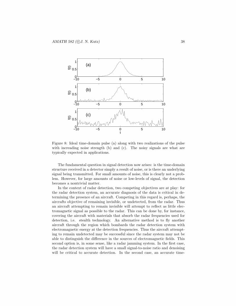
This will generate an ideal hyperbolic secant shape in the time domain. It isthis time domain signal that we will attempt to reconstruct via denoising andfiltering. Figure 8(a) illustrates the ideal signal.
In most applications, the signals as generated above are not ideal. Rather,they have a large amount of noise integrated within them. Usually this noiseis what is called white noise, i.e. a noise which effects all frequencies the same.We can add white noise to this signal by considering the pulse in the frequencydomain.
noise=1;
ut=fft(u);
utn=ut+noise*(randn(1,n)+i*randn(1,n));
un=ifft(utn);
figure(1), subplot(3,1,2), plot(t,abs(un),’k’), hold on
These three lines of code generate the Fourier transform of the function alongwith the vector utn which is the spectrum of the given signal with a complexand Gaussian distributed (mean zero, unit variance) noise source term addedin. Figure 8 shows the difference between the ideal time-domain signal pulseand the more physically realistic pulse for which white noise has been added. Inthese figures, a clear signal, i.e. the original time-domain pulse, is still detectedeven in the presence of noise.
AMATH 582 ( c©J. N. Kutz) 38
−10 −5 0 5 100
0.5
1
f(t) (a)
−10 −5 0 5 100
0.5
1
f(t) (b)
−10 −5 0 5 100
0.5
1
t
f(t) (c)
Figure 8: Ideal time-domain pulse (a) along with two realizations of the pulsewith increading noise strength (b) and (c). The noisy signals are what aretypically expected in applications.
The fundamental question in signal detection now arises: is the time-domainstructure received in a detector simply a result of noise, or is there an underlyingsignal being transmitted. For small amounts of noise, this is clearly not a prob-lem. However, for large amounts of noise or low-levels of signal, the detectionbecomes a nontrivial matter.
In the context of radar detection, two competing objectives are at play: forthe radar detection system, an accurate diagnosis of the data is critical in de-termining the presence of an aircraft. Competing in this regard is, perhaps, theaircrafts objective of remaining invisible, or undetected, from the radar. Thusan aircraft attempting to remain invisible will attempt to reflect as little elec-tromagnetic signal as possible to the radar. This can be done by, for instance,covering the aircraft with materials that absorb the radar frequencies used fordetection, i.e. stealth technology. An alternative method is to fly anotheraircraft through the region which bombards the radar detection system withelectromagnetic energy at the detection frequencies. Thus the aircraft attempt-ing to remain undetected may be successful since the radar system may not beable to distinguish the difference in the sources of electromagnetic fields. Thissecond option is, in some sense, like a radar jamming system. In the first case,the radar detection system will have a small signal-to-noise ratio and denoisingwill be critical to accurate detection. In the second case, an accurate time-

AMATH 582 ( c©J. N. Kutz) 39
−30 −20 −10 0 10 20 300
0.5
1
1.5
2
time (t)
|u|
−25 −20 −15 −10 −5 0 5 10 15 20 250
0.2
0.4
0.6
0.8
1
wavenumber (k)
|ut|/
max
(|ut
|)
Figure 9: Time-domain (top) and frequency-domain (bottom) plots for a singlerealization of white-noise. In this case, the noise strength has been increased toten, thus burying the desired signal field in both time and frequency.
frequency analysis is critical for determining the time localization and positionsof the competing signals.
The focus of what follows is to apply the ideas of spectral filtering to attemptto improve the signal detection by denoising. Spectral filtering is a methodwhich allows us to extract information at specific frequencies. For instance, inthe radar detection problem, it is understood that only a particular frequency(the emitted signal frequency) is of interest at the detector. Thus it would seemreasonable to filter out, in some appropriate manner, the remaining frequencycomponents of the electromagnetic field received at the detector.
Consider a very noisy field created around the hyperbolic secant of the pre-vious example (See Fig. 9):
noise=10;
ut=fft(u);
unt=ut+noise*(randn(1,n)+i*randn(1,n));
un=ifft(unt);
subplot(2,1,1), plot(t,abs(un),’k’)
axis([-30 30 0 2])

AMATH 582 ( c©J. N. Kutz) 40
−25 −20 −15 −10 −5 0 5 10 15 20 250
0.5
1
wavenumber (k)
|ut|/
max
(|ut
|)
−25 −20 −15 −10 −5 0 5 10 15 20 250
0.5
1
wavenumber (k)
|ut|/
max
(|ut
|)
−30 −20 −10 0 10 20 300
0.5
1
time (t)
|u|
Figure 10: (top) White-noise inundated signal field in the frequency domainalong with a Gaussian filter with bandwidth parameter τ = 0.2 centered on thesignal center frequency. (middle) The post-filtered signal field in the frequencydomain. (bottom) The time-domain reconstruction of the signal field (boldedline) along with the ideal signal field (light line) and the detection threshold ofthe radar (dotted line).
xlabel(’time (t)’), ylabel(’|u|’)
subplot(2,1,2)
plot(fftshift(k),abs(fftshift(unt))/max(abs(fftshift(unt))),’k’)
axis([-25 25 0 1])
xlabel(’wavenumber (k)’, ylabel(’|ut|/max(|ut|)’)
Figure 9 demonstrates the impact of a large noise applied to the underlyingsignal. In particular, the signal is completely buried within the white-noisefluctuations, making the detection of a signal difficult, if not impossible, withthe unfiltered noisy signal field.
Filtering can help significantly improve the ability to detect the signal buriedin the noisy field of Fig. 9. For the radar application, the frequency (wavenum-ber) of the emitted and reflected field is known, thus spectral filtering aroundthis frequency can remove undesired frequencies and much of the white-noisepicked up in the detection process. There are a wide range of filters that canbe applied to such a problem. One of the simplest filters to consider here is the

AMATH 582 ( c©J. N. Kutz) 41
Gaussian filter (See Fig. 10):
F(k) = exp(−τ(k − k0)2) (2.2.1)
where τ measures the bandwidth of the filter, and k is the wavenumber. Thegeneric filter function F(k) in this case acts as a low-pass filter since it eliminateshigh-frequency components in the system of interest. Note that these are high-frequencies in relation to the center-frequency (k = k0) of the desired signalfield. In the example considered here k0 = 0.
Application of the filter attenuates strongly those frequencies away fromcenter frequency k0. Thus if there is a signal near k0, the filter isolates thesignal input around this frequency or wavenumber. Application of the filteringresults in the following spectral processing in MATLAB:
filter=exp(-0.2*(k).^2);
unft=filter.*unt;
unf=ifft(unft);
The application of these lines of code are illustrate in Fig. 10 where the white-noise inundated signal field in the spectral domain is filtered with a Gaussianfilter centered around the zero wavenumber k0 = 0 with a bandwidth parameterτ = 0.2. The filtering extracts nicely the signal field despite the strength ofthe applied white-noise. Indeed, Fig. 10 (bottom) illustrates the effect of thefiltering process and its ability to reproduce an approximation to the signal field.In addition to the extracted signal field, a detection threshold is placed (dottedline) on the graph in order to illustrate that detector would read the extractedsignal as a target.
As a matter of completeness, the extraction of the electromagnetic field isalso illustrated when not centered on the center frequency. Figure 11 shows thefield that is extracted for a filter centered around k0 = 15. This is done easilywith the MATLAB commands
filter=exp(-0.2*(k-15).^2);
unft=filter.*unt;
unf=ifft(unft);
In this case, there is no signal around the wavenumber k0 = 15. However, there isa great deal of white-noise electromagnetic energy around this frequency. Uponfiltering and inverting the Fourier transform, it is clear from Figure 11 (bottom)that there is no discernible target present. As before, a decision threshold is setat |u| = 0.5 and the white noise fluctuations clearly produce a field well belowthe threshold line.
In all of the analysis above, filtering is done on a given set of signal data.However, the signal data is evolving in time, i.e. the position of the aircraftis probably moving. Moreover, one can imagine that there is some statistical

AMATH 582 ( c©J. N. Kutz) 42
−25 −20 −15 −10 −5 0 5 10 15 20 250
0.5
1
wavenumber (k)
|ut|/
max
(|ut
|)
−25 −20 −15 −10 −5 0 5 10 15 20 250
0.5
1
wavenumber (k)
|ut|/
max
(|ut
|)
−30 −20 −10 0 10 20 300
0.5
1
time (t)
|u|
Figure 11: (top) White-noise inundated signal field in the frequency domainalong with a Gaussian filter with bandwidth parameter τ = 0.2 centered on thesignal frequency k = 15. (middle) The post-filtered signal field in the frequencydomain. (bottom) The time-domain reconstruction of the signal field (boldedline) along the detection threshold of the radar (dotted line).
chance that a type I or type II error can be made in the detection. Thus atarget may be identified when there is no target, or a target has been missedcompletely. Ultimately, the goal is to use repeated measurements from the radarof the airspace in order to try to avoid a detection error or failure. Given thatyou may launch a missile, the stakes are high and a high level of confidenceis needed in the detection process. It should also be noted that filter design,shape, and parameterization play significant roles in designing optimal filters.Thus filter design is an object of strong interest in signal processing applications.
2.3 FFT Application: Radar Detection and Averaging
The last section clearly shows the profound and effective use of filtering in clean-ing up a noisy signal. This is one of the most basic illustrations of the powerbasic signal processing. Other methods also exist to help reduce noise and gen-erate better time-frequency resolution. In particular, the filtering example givenfails to use two key facts: the noise is white, and radar will continue to producemore signal data. These two facts can be used to produce useful information
AMATH 582 ( c©J. N. Kutz) 43
about the incoming signal. In particular, it is known, and demonstrated in thelast section, that white-noise can be modeled adding a normally distributedrandom variable with zero mean and unit variance to each Fourier componentof the spectrum. The key here: with zero mean. Thus if average over manysignals, the white-noise should, on average, add up to zero. A very simple con-cept, yet tremendously powerful in practice for signal processing systems wherethere is continuous detection of a signal.
To illustrate the power of denoising the system by averaging, the simpleanalysis of the last section will be considered for a time pulse. In beginning thisprocess, a time window must be selected and its Fourier resolution decided:
clear all; close all; clc
L=30; % total time slot
n=512; % Fourier modes
t2=linspace(-L,L,n+1); t=t2(1:n);
k=(2*pi/(2*L))*[0:(n/2-1) -n/2:-1]; ks=fftshift(k);
noise=10;
In order to be more effective in plotting our spectral results, the Fourier compo-nents in the standard shifted frame (k) and its unshifted counterpart (ks) areboth produced. Further, the noise strength of the system is selected.
In the next portion of the code, the total number of data frames, or real-izations of the incoming signal stream, is considered. The word realizations isused here to help underscore the fact that for each data frame, a new realizationof the white-noise is produced. In the following code, one, two, five, and onehundred realizations are considered.
labels=[’(a)’;’(b)’;’(c)’;’(d)’];
realize=[1 2 5 100];
for jj=1:length(realize)
u=sech(t); ave=zeros(1,n);
ut=fft(u);
for j=1:realize(jj)
utn(j,:)=ut+noise*(randn(1,n)+i*randn(1,n));
ave=ave+utn(j,:);
dat(j,:)=abs(fftshift(utn(j,:)))/max(abs(utn(j,:)));
un(j,:)=ifft(utn(j,:));
end
ave=abs(fftshift(ave))/realize(jj);
subplot(4,1,jj)
plot(ks,ave/max(ave),’k’)

AMATH 582 ( c©J. N. Kutz) 44
−20 −15 −10 −5 0 5 10 15 200
0.5
1(a)
|fft(
u)|
−20 −15 −10 −5 0 5 10 15 200
0.5
1(b)
|fft(
u)|
−20 −15 −10 −5 0 5 10 15 200
0.5
1(c)
|fft(
u)|
−20 −15 −10 −5 0 5 10 15 200
0.5
1(d)
|fft(
u)|
frequency (k)
Figure 12: Average spectral content for (a) one, (b) two, (c) five and (d) onehundred realizations of the data. The dotted line in (d) represents the ideal,noise-free spectral signature.
set(gca,’Fontsize’,[15])
axis([-20 20 0 1])
text(-18,0.7,labels(jj,:),’Fontsize’,[15])
ylabel(’|fft(u)|’,’Fontsize’,[15])
end
hold on
plot(ks,abs(fftshift(ut))/max(abs(ut)),’k:’,’Linewidth’,[2])
set(gca,’Fontsize’,[15])
xlabel(’frequency (k)’)
Figure 12 demonstrates the averaging process in the spectral domain as a func-tion of the number of realizations. With one realization, it is difficult to deter-mine if there is a true signal, or if the entire spectrum is noise. Already after tworealizations, the center frequency structure starts to appear. Five realizationshas a high degree of discrimination between the noise and signal and 100 real-izations is almost exactly converged to the ideal, noise-free signal. As expected,the noise in the averaging process is eliminated upon averaging since its meanis zero. To view a few of the data realizations used in computing the averaging

AMATH 582 ( c©J. N. Kutz) 45
−20−10
010
20
1
2
3
4
5
6
7
80
0.51
frequency (k)
realization
|fft(
u)|
Figure 13: Typical time domain signals that would be produced in a signaldetection system. At different times of measurement, the added white-noisewould alter the signal stream significantly.
in Fig. 12, the first eight time domain signals used to compute the average for100 realizations is shown in Fig. 13. The following code is used to produce thewaterfall plot used:
figure(2)
waterfall(ks,1:8,dat(1:8,:)), colormap([0 0 0]), view(-15,80)
set(gca,’Fontsize’,[15],’Xlim’,[-28 28],’Ylim’,[1 8])
xlabel(’frequency (k)’), ylabel(’realization’),zlabel(’|fft(u)|’)
Figures 12 and 13 illustrate how the averaging process can ultimately extracta clean spectral signature. As a consequence, however, you completely loose thetime-domain dynamics. In other words, one could take the cleaned up spectrumof Fig. 12 and inverse the Fourier transform, but this would only give the averagetime domain signal, but not how it actually evolved over time. To consider thisproblem more concretely, consider the following bit of code that generates atime-varying signal shown in Fig. 14. There are a total of 21 realizations ofdata in this example.
slice=[0:0.5:10];
[T,S]=meshgrid(t,slice);
[K,S]=meshgrid(k,slice);

AMATH 582 ( c©J. N. Kutz) 46
−30 −20 −10 0 10 20 300
5
10012
time (t)realizations
|u|
−20 −10 0 10 200
5
100
0.51
frequency (k)realizations
|fft(
u)|
Figure 14: Ideal time-frequency behavior for a time-domain pulse that evolvesdynamically in time. The spectral signature remains unchanged as the pulsemoves over the time domain.
U=sech(T-10*sin(S)).*exp(i*0*T);
subplot(2,1,1)
waterfall(T,S,U), colormap([0 0 0]), view(-15,70)
set(gca,’Fontsize’,[15],’Xlim’,[-30 30],’Zlim’,[0 2])
xlabel(’time (t)’), ylabel(’realizations’), zlabel(’|u|’)
for j=1:length(slice)
Ut(j,:)=fft(U(j,:));
Kp(j,:)=fftshift(K(j,:));
Utp(j,:)=fftshift(Ut(j,:));
Utn(j,:)=Ut(j,:)+noise*(randn(1,n)+i*randn(1,n));
Utnp(j,:)=fftshift(Utn(j,:))/max(abs(Utn(j,:)));
Un(j,:)=ifft(Utn(j,:));
end
figure(3)
subplot(2,1,2)
waterfall(Kp,S,abs(Utp)/max(abs(Utp(1,:)))), colormap([0 0 0]), view(-15,70)
set(gca,’Fontsize’,[15],’Xlim’,[-28 28])
xlabel(’frequency (k)’), ylabel(’realizations’), zlabel(’|fft(u)|’)
AMATH 582 ( c©J. N. Kutz) 47
−30 −20 −10 0 10 20 300
5
10012
time (t)realizations
|u|
−20 −10 0 10 200
5
100
0.51
frequency (k)realizations
|fft(
u)|
Figure 15: A more physically realistic depiction of the time-domain and fre-quency spectrum as a function of the number of realizations. The goal is toextract the meaningful data buried within the noise.
If this was a radar problem, the movement of the signal would represent anaircraft moving in time. The spectrum, however, remains fixed at the trans-mitted signal frequency. Thus it is clear even at this point that averaging overthe frequency realizations produces a clean, localized signature in the frequencydomain, whereas averaging over the time-domain only smears out the evolvingtime-domain pulse.
The ideal pulse evolution in Fig. 14 is now inundated with white-noise asshown in Fig. 15. The noise is added to each realization, or data measurement,with the same strength as shown in Figs. 12 and 13. The following code plotsthe noise time-domain and spectral evolution:
figure(4)
subplot(2,1,1)
waterfall(T,S,abs(Un)), colormap([0 0 0]), view(-15,70)
set(gca,’Fontsize’,[15],’Xlim’,[-30 30],’Zlim’,[0 2])
xlabel(’time (t)’), ylabel(’realizations’), zlabel(’|u|’)
subplot(2,1,2)
waterfall(Kp,S,abs(Utnp)), colormap([0 0 0]), view(-15,70)
set(gca,’Fontsize’,[15],’Xlim’,[-28 28])
xlabel(’frequency (k)’), ylabel(’realizations’), zlabel(’|fft(u)|’)

AMATH 582 ( c©J. N. Kutz) 48
−30 −20 −10 0 10 20 300
0.2
0.4
0.6
0.8
time (t)
|u|
−20 −15 −10 −5 0 5 10 15 200
0.5
1
frequency (k)
|fft(
u)|
Figure 16: Averaged time-domain and spectral profiles for the 21 realizationsof data shown in Fig. 15. Even with a limited sampling, the spectral signatureat the center frequency is extracted.
The obvious question arises about how to cleanup the signal and whether some-thing meaningful can be extracted from the data or not. After all, there areonly 21 data slices to work with. The following code averages over the 21 datarealizations in both the time and frequency domains
figure(5)
Uave=zeros(1,n); Utave=zeros(1,n);
for j=1:length(slice)
Uave=Uave+Un(j,:);
Utave=Utave+Utn(j,:);
end
Uave=Uave/length(slice);
Utave=fftshift(Utave)/length(slice);
subplot(2,1,1)
plot(t,abs(Uave),’k’)
set(gca,’Fontsize’,[15])
xlabel(’time (t)’), ylabel(’|u|’)
subplot(2,1,2)
AMATH 582 ( c©J. N. Kutz) 49
plot(ks,abs(Utave)/max(abs(Utave)),’k’), hold on
plot(ks,abs(fftshift(Ut(1,:)))/max(abs(Ut(1,:))),’k:’,’Linewidt’,[2])
axis([-20 20 0 1])
set(gca,’Fontsize’,[15])
xlabel(’frequency (k)’), ylabel(’|fft(u)|’)
Figure 16 shows the results from the averaging process for a nonstationarysignal. The top graph shows that averaging over the time domain for a movingsignal produces no discernible signal. However, averaging over the frequencydomain produces a clear signature at the center-frequency of interest. Ideally,if more data is collected a better average signal is produced. However, in manyapplications, the acquisition of data is limited and decisions must be made uponwhat are essentially small sample sizes.
2.4 Time-Frequency Analysis: Windowed Fourier Trans-forms
The Fourier transform is one of the most important and foundational methodsfor the analysis of signals. However, it was realized very early on that Fouriertransform based methods had severe limitations. Specifically, when transform-ing a given time signal, it is clear that all the frequency content of the signalcan be captured with the transform, but the transform fails to capture themoment in time when various frequencies were actually exhibited. Figure 17shows a proto-typical signal that may be of interest to study. The signal S(t) isclearly comprised of various frequency components that are exhibited at differ-ent times. For instance, at the beginning of the signal, there are high frequencycomponents. In contrast, the middle of the signal has relatively low frequencyoscillations. If the signal represented music, then the beginning of the signalwould produce high notes while the middle would produce low notes. TheFourier transform of the signal contains all this information, but there is noindication of when the high or low notes actually occur in time. Indeed, bydefinition the Fourier transform eliminates all time-domain information sinceyou actually integrated out all time in Eq. (2.1.8).
The obvious question to arise is this: what is the Fourier transform good forin the context of signal processing? In the previous sections where the Fouriertransform was applied, the signal being investigated was fixed in frequency, i.e.a sonar or radar detector with a fixed frequency ω0. Thus for a given signal, thefrequency of interest did not shift in time. By then using different measurementsin time, a signal tracking algorithm could be constructed. Thus an implicit as-sumption was made about the invariance of the signal frequency. Ultimately,the Fourier transform is superb for one thing: characterizing stationary or peri-odic signals. Informally, a stationary signal is such that repeated measurementsof the signal in time yield an average value that does not change in time. Mostsignals, however, do not satisfy this criteria. A song, for instance, changes its
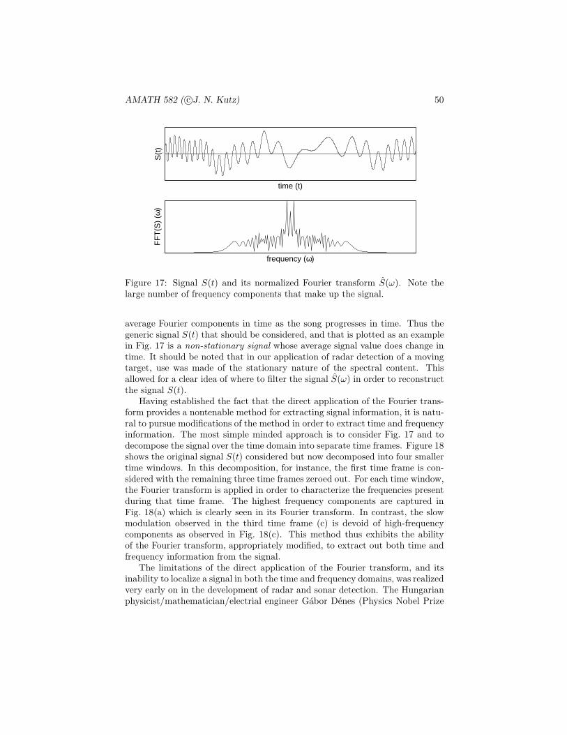
AMATH 582 ( c©J. N. Kutz) 50
S(t
)
time (t)
FF
T(S
) (ω
)
frequency (ω)
Figure 17: Signal S(t) and its normalized Fourier transform S(ω). Note thelarge number of frequency components that make up the signal.
average Fourier components in time as the song progresses in time. Thus thegeneric signal S(t) that should be considered, and that is plotted as an examplein Fig. 17 is a non-stationary signal whose average signal value does change intime. It should be noted that in our application of radar detection of a movingtarget, use was made of the stationary nature of the spectral content. Thisallowed for a clear idea of where to filter the signal S(ω) in order to reconstructthe signal S(t).
Having established the fact that the direct application of the Fourier trans-form provides a nontenable method for extracting signal information, it is natu-ral to pursue modifications of the method in order to extract time and frequencyinformation. The most simple minded approach is to consider Fig. 17 and todecompose the signal over the time domain into separate time frames. Figure 18shows the original signal S(t) considered but now decomposed into four smallertime windows. In this decomposition, for instance, the first time frame is con-sidered with the remaining three time frames zeroed out. For each time window,the Fourier transform is applied in order to characterize the frequencies presentduring that time frame. The highest frequency components are captured inFig. 18(a) which is clearly seen in its Fourier transform. In contrast, the slowmodulation observed in the third time frame (c) is devoid of high-frequencycomponents as observed in Fig. 18(c). This method thus exhibits the abilityof the Fourier transform, appropriately modified, to extract out both time andfrequency information from the signal.
The limitations of the direct application of the Fourier transform, and itsinability to localize a signal in both the time and frequency domains, was realizedvery early on in the development of radar and sonar detection. The Hungarianphysicist/mathematician/electrial engineer Gabor Denes (Physics Nobel Prize

AMATH 582 ( c©J. N. Kutz) 51
S(t
)
time (t)
(a) (b) (c) (d)
FF
T(S
) (ω
)
frequency (ω)
(a)
FF
T(S
) (ω
)
frequency (ω)
(b)
FF
T(S
) (ω
)
frequency (ω)
(c)F
FT
(S)
(ω)
frequency (ω)
(d)
Figure 18: Signal S(t) decomposed into four equal and separate time frames(a), (b), (c) and (d). The corresponding normalized Fourier transform of eachtime frame S(ω) is illustrated below the signal. Note that this decompositiongives information about the frequencies present in each smaller time frame.
in 1971 for the discovery of holography in 1947) was first to propose a formalmethod for localizing both time and frequency. His method involved a simplemodification of the Fourier transform kernel. Thus Gabor introduced the kernel
gt,ω(τ) = eiωτg(τ − t) (2.4.1)
where the new term to the Fourier kernel g(τ − t) was introduced with the aimof localizing both time and frequency. The Gabor transform, also known as theshort-time Fourier transform (STFT) is then defined as the following:
G[f ](t, ω) = fg(t, ω) =
∫ ∞
−∞
f(τ)g(τ − t)e−iωτdτ = (f, gt,ω) (2.4.2)
where the bar denotes the complex conjugate of the function. Thus the functiong(τ − t) acts as a time filter for localizing the signal over a specific window oftime. The integration over the parameter τ slides the time-filtering windowdown the entire signal in order to pick out the frequency information at eachinstant of time. Figure 19 gives a nice illustration of how the time filteringscheme of Gabor works. In this figure, the time filtering window is centered at

AMATH 582 ( c©J. N. Kutz) 52
|S(t
)|
time (t)
τa
Figure 19: Graphical depiction of the Gabor transform for extracting the time-frequency content of a signal S(t). The time filtering window g(τ−t) is centeredat τ with width a.
τ with a width a. Thus the frequency content of a window of time is extractedand τ is modified to extract the frequencies of another window. The definitionof the Gabor transform captures the entire time-frequency content of the signal.Indeed, the Gabor transform is a function of the two variables t and ω.
A few of the key mathematical properties of the Gabor transform are high-lighted here. To be more precise about these mathematical features, someassumptions about commonly used gt,ω are considered. Specifically, for con-venience we will consider g to be real and symmetric with ‖g(t)‖ = 1 and‖g(τ − t)‖ = 1 where ‖ · ‖ denotes the L2 norm. Thus the definition of theGabor transform, or STFT, is modified to
G[f ](t, ω) = fg(t, ω) =
∫ ∞
−∞
f(τ)g(τ − t)e−iωτdτ (2.4.3)
with g(τ − t) inducing localization of the Fourier integral around t = τ . Withthis definition, the following properties hold
1. The energy is bounded by the Schwarz inequality so that
|fg(t, ω)| ≤ ‖f‖‖g‖ (2.4.4)
2. The energy in the signal plane around the neighborhood of (t, ω) is calcu-lated from
|fg(t, ω)|2 =
∣∣∣∣∫ ∞
−∞
f(τ)g(τ − t)e−iωτdτ
∣∣∣∣2
(2.4.5)
3. The time-frequency spread around of a Gabor window is computed fromthe variance, or second moment, so that
σ2t =
∫ ∞
−∞
(τ − t)|gt,ω(τ)|2dτ =
∫ ∞
−∞
τ2|g(τ)|2dτ (2.4.6a)
σ2ω =
1
2π
∫ ∞
−∞
(ν − ω)2|gt,ω(ν)|2dν =1
2π
∫ ∞
−∞
ν2|g(ν)|2dν (2.4.6b)
where σtσω is independent of t and ω and is governed by the Heinsenberguncertainty principle.
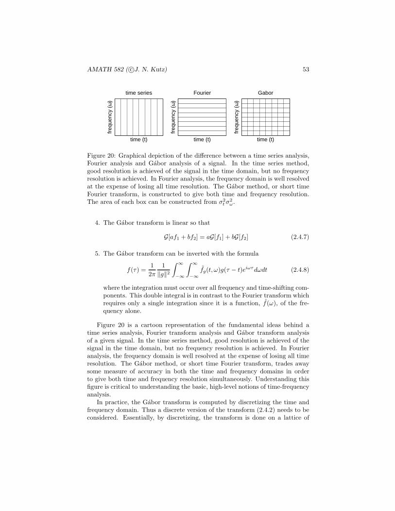
AMATH 582 ( c©J. N. Kutz) 53
time (t)
freq
uenc
y (ω
)
time series
time (t)
freq
uenc
y (ω
)
Fourier
time (t)
freq
uenc
y (ω
)
Gabor
Figure 20: Graphical depiction of the difference between a time series analysis,Fourier analysis and Gabor analysis of a signal. In the time series method,good resolution is achieved of the signal in the time domain, but no frequencyresolution is achieved. In Fourier analysis, the frequency domain is well resolvedat the expense of losing all time resolution. The Gabor method, or short timeFourier transform, is constructed to give both time and frequency resolution.The area of each box can be constructed from σ2
t σ2ω.
4. The Gabor transform is linear so that
G[af1 + bf2] = aG[f1] + bG[f2] (2.4.7)
5. The Gabor transform can be inverted with the formula
f(τ) =1
2π
1
‖g‖2
∫ ∞
−∞
∫ ∞
−∞
fg(t, ω)g(τ − t)eiωτdωdt (2.4.8)
where the integration must occur over all frequency and time-shifting com-ponents. This double integral is in contrast to the Fourier transform whichrequires only a single integration since it is a function, f(ω), of the fre-quency alone.
Figure 20 is a cartoon representation of the fundamental ideas behind atime series analysis, Fourier transform analysis and Gabor transform analysisof a given signal. In the time series method, good resolution is achieved of thesignal in the time domain, but no frequency resolution is achieved. In Fourieranalysis, the frequency domain is well resolved at the expense of losing all timeresolution. The Gabor method, or short time Fourier transform, trades awaysome measure of accuracy in both the time and frequency domains in orderto give both time and frequency resolution simultaneously. Understanding thisfigure is critical to understanding the basic, high-level notions of time-frequencyanalysis.
In practice, the Gabor transform is computed by discretizing the time andfrequency domain. Thus a discrete version of the transform (2.4.2) needs to beconsidered. Essentially, by discretizing, the transform is done on a lattice of
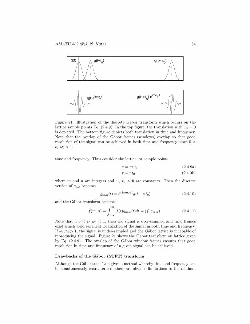
AMATH 582 ( c©J. N. Kutz) 54
g(t) g(t−t0) g(t−nt
0)
g(t)eimω0 t g(t−nt
0) eimω
0 t
Figure 21: Illustration of the discrete Gabor transform which occurs on thelattice sample points Eq. (2.4.9). In the top figure, the translation with ω0 = 0is depicted. The bottom figure depicts both translation in time and frequency.Note that the overlap of the Gabor frames (windows) overlap so that goodresolution of the signal can be achieved in both time and frequency since 0 <t0, ω0 < 1.
time and frequency. Thus consider the lattice, or sample points,
ν = mω0 (2.4.9a)
τ = nt0 (2.4.9b)
where m and n are integers and ω0, t0 > 0 are constants. Then the discreteversion of gt,ω becomes
gm,n(t) = ei2πmω0tg(t− nt0) (2.4.10)
and the Gabor transform becomes
f(m,n) =
∫ ∞
−∞
f(t)gm,n(t)dt = (f, gm,n) . (2.4.11)
Note that if 0 < t0, ω0 < 1, then the signal is over-sampled and time framesexist which yield excellent localization of the signal in both time and frequency.If ω0, t0 > 1, the signal is under-sampled and the Gabor lattice is incapable ofreproducing the signal. Figure 21 shows the Gabor transform on lattice givenby Eq. (2.4.9). The overlap of the Gabor window frames ensures that goodresolution in time and frequency of a given signal can be achieved.
Drawbacks of the Gabor (STFT) transform
Although the Gabor transform gives a method whereby time and frequency canbe simultaneously characterized, there are obvious limitations to the method.
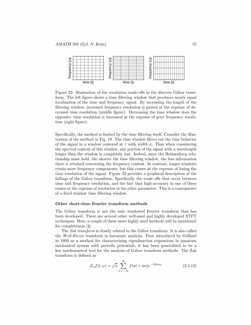
AMATH 582 ( c©J. N. Kutz) 55
time (t)
freq
uenc
y (ω
)
time (t)
freq
uenc
y (ω
)
time (t)
freq
uenc
y (ω
)
Figure 22: Illustration of the resolution trade-offs in the discrete Gabor trans-form. The left figure shows a time filtering window that produces nearly equallocalization of the time and frequency signal. By increasing the length of thefiltering window, increased frequency resolution is gained at the expense of de-creased time resolution (middle figure). Decreasing the time window does theopposite: time resolution is increased at the expense of poor frequency resolu-tion (right figure).
Specifically, the method is limited by the time filtering itself. Consider the illus-tration of the method in Fig. 19. The time window filters out the time behaviorof the signal in a window centered at τ with width a. Thus when consideringthe spectral content of this window, any portion of the signal with a wavelengthlonger than the window is completely lost. Indeed, since the Heinsenberg rela-tionship must hold, the shorter the time filtering window, the less informationthere is retained concerning the frequency content. In contrast, longer windowsretain more frequency components, but this comes at the expense of losing thetime resolution of the signal. Figure 22 provides a graphical description of thefailings of the Gabor transform. Specifically the trade offs that occur betweentime and frequency resolution, and the fact that high-accuracy in one of thesecomes at the expense of resolution in the other parameter. This is a consequenceof a fixed window time filtering window.
Other short-time Fourier transform methods
The Gabor transform is not the only windowed Fourier transform that hasbeen developed. There are several other well-used and highly developed STFTtechniques. Here, a couple of these more highly used methods will be mentionedfor completeness [4].
The Zak transform is closely related to the Gabor transform. It is also calledthe Weil-Brezin transform in harmonic analysis. First introduced by Gelfandin 1950 as a method for characterizing eigenfunction expansions in quantummechanical system with periodic potentials, it has been generalized to be akey mathematical tool for the analysis of Gabor transform methods. The Zaktransform is defined as
Laf(t, ω) =√a
∞∑
n=−∞
f(at+ an)e−i2πnω (2.4.12)

AMATH 582 ( c©J. N. Kutz) 56
where a > 0 is a constant and n is an integer. Two useful and key properties ofthis transform are as follows: Lf(t, ω + 1) = Lf(t, ω) (periodicity) and Lf(t +1, ω) = exp(i2πω)Lf(t, ω) (quasi-periodicity). These properties are particularlyimportant for considering physical problems placed on a lattice.
The Wigner-Ville Distribution is particularly important transform in the de-velopment of radar and sonar technologies. Its various mathematical propertiesmake it ideal for these applications and provides a method for achieving greattime and frequency localization. The Wigner-Ville transform is defined as
Wf,g(t, ω) =
∫ ∞
−∞
f(t+ τ/2)g(t− τ/2)e−iωτdτ (2.4.13)
where this is a standard Fourier kernel which transforms the function f(t +τ/2)g(t − τ/2). This transform is nonlinear since Wf1+f2,g1+g2 = Wf1,g1 +Wf1,g2 + Wf2,g1 + Wf2,g2 and Wf+g = Wf + Wg + 2ℜ{Wf,g}.
Ultimately, alternative forms of the STFT are developed for one specificreason: to take advantage of some underlying properties of the physical ormathematical properties of a given system. It is rare that a method developedfor radar would be broadly applicable to other physical systems unless theywere operating under the same physical principles. Regardless, one can see thatspecialty techniques exist for time-frequency analysis of different systems.
2.5 Time-Frequency Analysis and Wavelets
The Gabor transform established two key principles for joint time-frequencyanalysis: translation of a short-time window and scaling of the short-time win-dow to capture finer time resolution. Figure 19 shows the basic concept intro-duced in the theory of windowed Fourier transforms. Two parameters are intro-duced to handle the translation and scaling, namely τ and a. The shortcomingof this method is that it trades off accuracy in time (frequency) for accuracy infrequency (time). Thus the fixed window size imposes a fundamental limitationon the level of time-frequency resolution that can be obtained.
A simple modification to the Gabor method is to allow the scaling window(a) to vary in order to successively extract extract out improvements in thetime resolution. In other words, first the low-frequency (poor time resolution)components are extracted using a broad scaling window. The scaling windowis subsequently shortened in order to extract out higher-frequencies and bettertime resolution. By keeping a catalogue of the extracting process, both excellenttime and frequency resolution of a given signal can be obtained. This is thefundamental principle of wavelet theory. The term wavelet means little waveand originates from the fact that the scaling window extracts out smaller andsmaller pieces of waves from the larger signal.
Wavelet analysis begins with the consideration of a function known as the

AMATH 582 ( c©J. N. Kutz) 57
0 0.5 1
−1
0
1
time (t)
ψ
−100 −50 0 50 1000
0.4
0.8
frequency (ω)
FF
T(
ψ )
Figure 23: Representation of the compactly supported Haar wavelet functionψ(t) and its Fourier transform ψ(ω). Although highly localized in time due tothe compact support, it is poorly localized in frequency with a decay of 1/ω.
mother wavelet:
ψa,b(t) =1√aψ
(t− b
a
)(2.5.14)
where a 6= 0 and b are real constants. The parameter a is the scaling parameterillustrated in Fig. 19 whereas the parameter b now denotes the translation pa-rameter (previously denoted by τ in Fig. 19). Unlike Fourier analysis, and verymuch like Gabor transforms, there are a vast variety of mother wavelets thatcan be constructed. In principle, the mother wavelet is designed to have certainproperties that are somehow beneficial for a given problem. Thus dependingupon the application, different mother wavelets may be selected.
Ultimately, the wavelet is simply another expansion basis for representinga given signal or function. Thus it is not unlike the Fourier transform whichrepresents the signal as a series of sines and cosines. Historically, the firstwavelet was constructed by Haar in 1910 [5]. Thus the concepts and ideas ofwavelets are one century old. However, their widespread use and applicationdid not become prevalent until the mid-1980s. The Haar wavelet is given by thepiecewise constant function
ψ(t) =
1 0 ≤ t < 1/2−1 1/2 ≤ t < 10 otherwise
. (2.5.15)
Figure 23 shows the Haar wavelet step function and its Fourier transform whichis a sinc like function. Note further that
∫ ∞
−∞ψ(t)dt = 0 and ‖ψ(t)‖2 =∫ ∞
−∞|ψ(t)|2dt. The Haar wavelet is an ideal wavelet for describing localized
signals in time (or space) since it has compact support. Indeed, for highly local-ized signals, it is a much more efficient to use the Haar wavelet basis than thestandard Fourier expansion. However. the Haar wavelet has poor localizationproperties in the frequency domain since it decays like a sinc function in powersof 1ω. This is a consequence of the Heinsenberg uncertainty principle.
To represent a signal with the Haar wavelet basis, the translation and scalingoperations associated with the mother wavelet need to be considered. Depicted

AMATH 582 ( c©J. N. Kutz) 58
0 0.5−2
0
2
time (t)
ψ
−100 −50 0 50 1000
0.5
1
frequency (ω)
FF
T(
ψ )
0 1 2
−0.50
0.5
time (t)
ψ
−100 −50 0 50 1000
0.5
1
frequency (ω)
FF
T(
ψ )
Figure 24: Illustration of the compression and dilation process of the Haarwavelet and its Fourier transform. In the top row, the compressed wavelet ψ1/2,0
is shown. Improved time resolution is obtained at the expense of a broaderfrequency signature. The bottom row, shows the dilated wavelet ψ2,0 whichallows it to capture lower-frequency components of a signal.
in Fig. 23 and given by Eq. (2.5.15) is the wavelet ψ1,0(t). Thus its translationis zero and its scaling is unity. The concept in reconstructing a signal usingthe Haar wavelet basis is to consider decomposing the signal into more genericψm,n(t). By appropriate selection of the m and n (integers), finer scales andappropriate locations of the signal can be extracted. For a < 1, the wavelet isa compressed version of ψ1,0 whereas for a > 1, the wavelet is a dilated versionof ψ1,0. The scaling parameter a is typically taken to be a power of two sothat a = 2j for some integer j. Figure 24 shows the compressed and dilatedHaar wavelet for a = 0.5 and a = 2, i.e. ψ1/2,0 and ψ2,0. The compressedwavelet allows for finer scale resolution of a given signal while the dilated waveletcaptures low-frequency components of a signal by having a broad range in time.
The simple Haar wavelet already illustrates all the fundamental principlesof the wavelet concept. Specifically by using scaling and translation, a givensignal or function can be represented by a basis of functions which allow forhigher and higher refinement in the time resolution of a signal. Thus it ismuch like the Gabor concept, except that now the time window is variable inorder to capture different levels of resolution. Thus the large scale structuresin time are captured with broad time-domain Haar wavelets. At this scale, thetime resolution of the signal is very poor. However by successive rescaling intime, a finer and finer time resolution of the signal can be obtained along withits high-frequency components. The information at the low and high scales isall preserved so that a complete picture of the time-frequency domain can beconstructed. Ultimately, the only limit in this process is the number of scalinglevels to be considered.

AMATH 582 ( c©J. N. Kutz) 59
The wavelet basis can be accessed via an integral transform of the form
(Tf)(ω) =
∫
t
K(t, ω)f(t)dt (2.5.16)
where K(t, ω) is the kernel of the transform. This is equivalent in principleto the Fourier transform whose kernel are the oscillations given by K(t, ω) =exp(−iωt). The key idea now is to define a transform which incorporates themother wavelet as the kernel. Thus we define the continuous wavelet transform(CWT):
Wψ[f ](a, b) = (f, ψa,b) =
∫ ∞
−∞
f(t)ψa,b(t)dt (2.5.17)
Much like the windowed Fourier transform, the CWT is a function of the di-lation parameter a and translation parameter b. Parenthetically, a wavelet isadmissible if the following property holds:
Cψ =
∫ ∞
−∞
|ψ(ω)|2|ω| dω <∞ (2.5.18)
where the Fourier transform of the wavelet is defined by
ψa,b =1√|a|
∫ ∞
−∞
e−iωtψ
(t− b
a
)dt =
1√|a|e−ibωψ(aω) . (2.5.19)
Thus provided the admissibility condition (2.5.18) is satisfied, the wavelet trans-form can be well defined.
As an example of the admissibility condition, consider the Haar wavelet(2.5.15). Its Fourier transform can be easily computed in terms of the sinc-likefunction:
ψ(ω) = ie−iω/2sin2(ω/4)
ω/4. (2.5.20)
Thus the admissibility constant can be computed to be
∫ ∞
−∞
|ψ(ω)|2|ω| dω = 16
∫ ∞
−∞
1
|ω|3∣∣∣sin ω
4
∣∣∣4
dω <∞ . (2.5.21)
This then shows that the Haar wavelet is in the admissible class.Another interesting properties of the wavelet transform is the ability to con-
struct new wavelet bases. The following theorem is of particular importance.
Theorem: If ψ is a wavelet and φ is a bounded integrable function, then theconvolution ψ ⋆ φ is a wavelet.
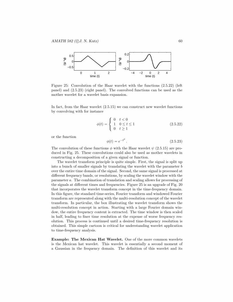
AMATH 582 ( c©J. N. Kutz) 60
0 1 2
−0.5
0
0.5
time (t)
(ψ *
φ)
−4 −2 0 2 4−0.2
0
0.2
time (t)
(ψ *
φ)
Figure 25: Convolution of the Haar wavelet with the functions (2.5.22) (leftpanel) and (2.5.23) (right panel). The convolved functions can be used as themother wavelet for a wavelet basis expansion.
In fact, from the Haar wavelet (2.5.15) we can construct new wavelet functionsby convolving with for instance
φ(t) =
0 t < 01 0 ≤ t ≤ 10 t ≥ 1
(2.5.22)
or the functionφ(t) = e−t
2
. (2.5.23)
The convolution of these functions φ with the Haar wavelet ψ (2.5.15) are pro-duced in Fig. 25. These convolutions could also be used as mother wavelets inconstructing a decomposition of a given signal or function.
The wavelet transform principle is quite simple. First, the signal is split upinto a bunch of smaller signals by translating the wavelet with the parameter bover the entire time domain of the signal. Second, the same signal is processed atdifferent frequency bands, or resolutions, by scaling the wavelet window with theparameter a. The combination of translation and scaling allows for processing ofthe signals at different times and frequencies. Figure 25 is an upgrade of Fig. 20that incorporates the wavelet transform concept in the time-frequency domain.In this figure, the standard time-series, Fourier transform and windowed Fouriertransform are represented along with the multi-resolution concept of the wavelettransform. In particular, the box illustrating the wavelet transform shows themulti-resolution concept in action. Starting with a large Fourier domain win-dow, the entire frequency content is extracted. The time window is then scaledin half, leading to finer time resolution at the expense of worse frequency res-olution. This process is continued until a desired time-frequency resolution isobtained. This simple cartoon is critical for understanding wavelet applicationto time-frequency analysis.
Example: The Mexican Hat Wavelet. One of the more common waveletsis the Mexican hat wavelet. This wavelet is essentially a second moment ofa Gaussian in the frequency domain. The definition of this wavelet and its
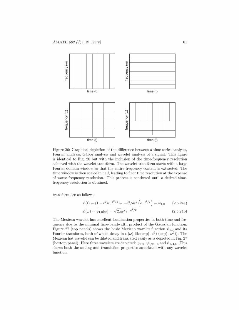
AMATH 582 ( c©J. N. Kutz) 61
time (t)
freq
uenc
y (ω
)
time (t)
freq
uenc
y (ω
)
time (t)
freq
uenc
y (ω
)
time (t)
freq
uenc
y (ω
)
Figure 26: Graphical depiction of the difference between a time series analysis,Fourier analysis, Gabor analysis and wavelet analysis of a signal. This figureis identical to Fig. 20 but with the inclusion of the time-frequency resolutionachieved with the wavelet transform. The wavelet transform starts with a largeFourier domain window so that the entire frequency content is extracted. Thetime window is then scaled in half, leading to finer time resolution at the expenseof worse frequency resolution. This process is continued until a desired time-frequency resolution is obtained.
transform are as follows:
ψ(t) = (1 − t2)e−t2/2 = −d2/dt2
(e−t
2/2)
= ψ1,0 (2.5.24a)
ψ(ω) = ψ1,0(ω) =√
2πω2e−ω2/2 (2.5.24b)
The Mexican wavelet has excellent localization properties in both time and fre-quency due to the minimal time-bandwidth product of the Gaussian function.Figure 27 (top panels) shows the basic Mexican wavelet function ψ1,0 and itsFourier transform, both of which decay in t (ω) like exp(−t2) (exp(−ω2)). TheMexican hat wavelet can be dilated and translated easily as is depicted in Fig. 27(bottom panel). Here three wavelets are depicted: ψ1,0, ψ3/2,−3 and ψ1/4,6. Thisshows both the scaling and translation properties associated with any waveletfunction.

AMATH 582 ( c©J. N. Kutz) 62
−6 −3 0 3 6−0.5
0
0.5
1
time (t)
ψ(a)
−10 −5 0 5 100
1
2
frequency (ω)
FF
T(
ψ )
(b)
−8 −4 0 4 8−1
0
1
2
time (t)
ψ1,0
ψ3/2,−3
ψ1/4,6(c)
Figure 27: Illustration of the Mexican hat wavelet ψ1,0 (top left panel), its
Fourier transform ψ1,0 (top right panel), and two additional dilations and trans-lations of the basic ψ1,0 wavelet. Namely the ψ3/2,−3 and ψ1/4,6 are shown(bottom panel).
To finish the initial discussion of wavelets, some of the various propertiesof the wavelets are discussed. To begin, consider the time-frequency resolutionand its localization around a given time and frequency. These quantities can becalculated from the relations:
σ2t =
∫ ∞
−∞
(t− < t >)2|ψ(t)|2dt (2.5.25a)
σ2ω =
1
2π
∫ ∞
−∞
(ω− < ω >)2|ψ(ω)|2dω (2.5.25b)
where the variances measure the spread of the time and frequency signal around< t > and < ω > respectively. The Heisenberg uncertainty constrains thelocalization of time and frequency by the relation σ2
t σ2ω ≥ 1/2. In addition, the
CWT has the following mathematical properties
1. Linearity: the transform is linear so that
Wψ(αf + βg)(a, b) = αWψ(f)(a, b) + βWψ(g)(a, b)
2. Translation: the transform has the translation property
Wψ(Tcf)(a, b) = Wψ(f)(a, b− c)
where Tcf(t) = f(t− c).
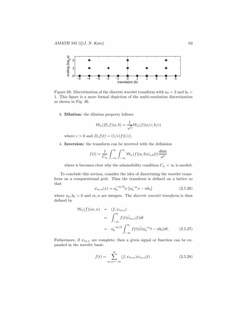
AMATH 582 ( c©J. N. Kutz) 63
−5 −4 −3 −2 −1 0 1 2 3 4 50
1
2
translation (b)
scal
ing
(log 2a)
Figure 28: Discretization of the discrete wavelet transform with a0 = 2 and b0 =1. This figure is a more formal depiction of the multi-resolution discretizationas shown in Fig. 26.
3. Dilation: the dilation property follows
Wψ(Dcf)(a, b) =1√cWψ(f)(a/c, b/c)
where c > 0 and Dcf(t) = (1/c)f(t/c).
4. Inversion: the transform can be inverted with the definision
f(t) =1
Cψ
∫ ∞
−∞
∫ ∞
−∞
Wψ(f)(a, b)ψa,b(t)dbda
a2
where is becomes clear why the admissibility condition Cψ <∞ is needed.
To conclude this section, consider the idea of discretizing the wavelet trans-form on a computational grid. Thus the transform is defined on a lattice sothat
ψm,n(x) = a−m/20 ψ
(a−m0 x− nb0
)(2.5.26)
where a0, b0 > 0 and m,n are integers. The discrete wavelet transform is thendefined by
Wψ(f)(m,n) = (f, ψm,n)
=
∫ ∞
−∞
f(t)ψm,n(t)dt
= a−m/20
∫ ∞
−∞
f(t)ψ(a−m0 t− nb0)dt . (2.5.27)
Futhermore, if ψm,n are complete, then a given signal or function can be ex-panded in the wavelet basis:
f(t) =
∞∑
m,n=−∞
(f, ψm,n)ψm,n(t) . (2.5.28)
AMATH 582 ( c©J. N. Kutz) 64
This expansion is in a set of wavelet frames. It still needs to be determinedif the expansion is in terms of a set of basis functions. It should be notedthat the scaling and dilation parameters are typically taken to be a0 = 2 andb0 = 1, corresponding to dilations of 2−m and translations of n2m. Figure 28gives a graphical depiction of the time-frequency discretization of the wavelettransform. This figure is especially relevant for the computational evaluationof the wavelet transform. Further, it is the basis of fast algorithms for multi-resolution analysis.
2.6 Multi-Resolution Analysis and the Wavelet Basis
Before proceeding forward with wavelets, it is important to establish some keymathematical properties. Indeed, the most important issue to resolve is theability of the wavelet to actually represent a given signal or function. In Fourieranalysis, it has been established that any generic function can be represented bya series of cosines and sines. Something similar is needed for wavelets in orderto make them a useful tool for the analysis of time-frequency signals.
The concept of a wavelet is simple and intuitive: construct a signal using asingle function ψ ∈ L2 which can be written ψm,n and that represents binarydilations by 2m and translations of n2−m so that
ψm,n = 2m/2ψ (2m(x− n/2m)) = 2m/2ψ(2mx− n) (2.6.29)
where m and n are integers. The use of this wavelet for representing a givensignal or function is simple enough. However, there is a critical issue to beresolved concerning the orthogonality of the functions ψm,n. Ultimately, this isthe primary issue which must be addressed in order to consider the wavelets asbasis functions in an expansion. Thus we define the orthogonality condition as
(ψm,n, ψk,l) =
∫ ∞
−∞
ψm,n(x)ψk,l(x)dx = δm,kδn,l (2.6.30)
where δij is the Dirac delta defined by
δij =
{0 i 6= j1 i = j
(2.6.31)
where i, j are integers. This statement of orthogonality is generic and in mostfunctional spaces with a defined inner product.
The importance of orthogonality should not be underestimated. It is veryimportant in applications where a functional expansion is used to approximatea given function or solution. In what follows, two examples are given concerningthe key role of orthogonality.
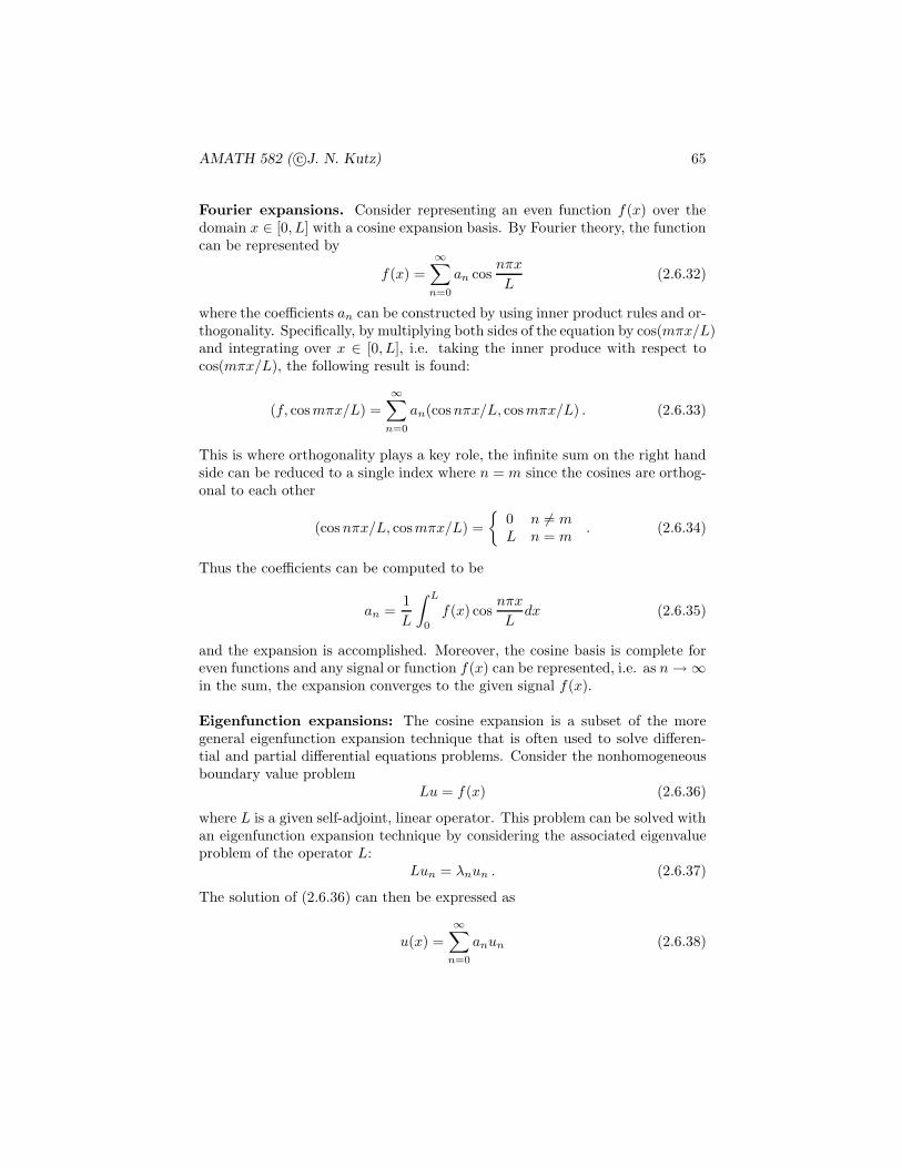
AMATH 582 ( c©J. N. Kutz) 65
Fourier expansions. Consider representing an even function f(x) over thedomain x ∈ [0, L] with a cosine expansion basis. By Fourier theory, the functioncan be represented by
f(x) =
∞∑
n=0
an cosnπx
L(2.6.32)
where the coefficients an can be constructed by using inner product rules and or-thogonality. Specifically, by multiplying both sides of the equation by cos(mπx/L)and integrating over x ∈ [0, L], i.e. taking the inner produce with respect tocos(mπx/L), the following result is found:
(f, cosmπx/L) =
∞∑
n=0
an(cosnπx/L, cosmπx/L) . (2.6.33)
This is where orthogonality plays a key role, the infinite sum on the right handside can be reduced to a single index where n = m since the cosines are orthog-onal to each other
(cosnπx/L, cosmπx/L) =
{0 n 6= mL n = m
. (2.6.34)
Thus the coefficients can be computed to be
an =1
L
∫ L
0
f(x) cosnπx
Ldx (2.6.35)
and the expansion is accomplished. Moreover, the cosine basis is complete foreven functions and any signal or function f(x) can be represented, i.e. as n→ ∞in the sum, the expansion converges to the given signal f(x).
Eigenfunction expansions: The cosine expansion is a subset of the moregeneral eigenfunction expansion technique that is often used to solve differen-tial and partial differential equations problems. Consider the nonhomogeneousboundary value problem
Lu = f(x) (2.6.36)
where L is a given self-adjoint, linear operator. This problem can be solved withan eigenfunction expansion technique by considering the associated eigenvalueproblem of the operator L:
Lun = λnun . (2.6.37)
The solution of (2.6.36) can then be expressed as
u(x) =
∞∑
n=0
anun (2.6.38)

AMATH 582 ( c©J. N. Kutz) 66
provided the coefficients an can be determined. Plugging in this solution to(2.6.36) yields the following calculations
Lu = f
L(∑
anun) = f∑
anLun = f∑
anλnun = f . (2.6.39)
Taking the inner product of both sides with respect to um yields
(∑
anλnun, um) = (f, um)∑
anλn(un, um) = (f, um)
amλm = (f, um) (2.6.40)
where the last line is achieved by orthogonality of the eigenfunctions (un, um) =δn,m. This then gives am = (f, um)/λm and the eigenfunction expansion solu-tion is
u(x) =
∞∑
n=0
(f, un)
λnun . (2.6.41)
Provided the un are a complete set, this expansion is guaranteed to converge tou(x) as n→ ∞.
Orthonormal wavelets
The preceding examples highlight the importance of orthogonality for represent-ing a given function. A wavelet ψ is called orthogonal if the family of functionsψm,n are orthogonal as given by Eq. (2.6.30). In this case, a given signal orfunction can be uniquely expressed with the doubly infinite series
f(t) =
∞∑
n,m=−∞
cm,nψm,n(t) (2.6.42)
where the coefficients are given from orthogonality by
cm,n = (f, ψm,n) . (2.6.43)
The series is guaranteed to converge to f(t) in the L2 norm.The above result based upon orthogonal wavelets establishes the key math-
ematical framework needed for using wavelets in a very broad and general way.It is this result that allows us to think of wavelets philosophically as the sameas the Fourier transform.

AMATH 582 ( c©J. N. Kutz) 67
Multi-Resolution Analysis (MRA)
The power of the wavelet basis is its ability to take a function or signal f(t)and express it as a limit of successive approximations, each of which is a finerand finer version of the function in time. These successive approximations cor-respond to different resolution levels.
A multi-resolution analysis, commonly referred to as an MRA, is a methodthat gives a formal approach to constructing the signal with different resolutionlevels. Mathematically, this involves a sequence
{Vm : m ∈ integers} (2.6.44)
of embedded subspaces of L2 that satisfies the following relations:
1. The subspaces can be embedded in each other so that
· · · ⊂ V−2 ⊂ V−1 ⊂ V0 ⊂ V1 ⊂ V2 · · ·Vm ⊂ Vm+1 · · ·
2. The union of all the embedded subspaces spans the entire L2 space so that
∪∞m=−∞Vm
is dense in L2
3. The intersection of subspaces is the null set so that
∩∞m=−∞Vm = {0}
4. Each subspace picks up a given resolution so that f(x) ∈ Vm if and onlyif f(2x) ∈ Vm+1 for all integers m.
5. There exists a function φ ∈ V0 such that
{φ0,n = φ(x −m)}
is an orthogonal basis for V0 so that
‖f‖2 =
∫ ∞
−∞
|f(x)|2dx =∞∑
−∞
|(f, φ0,n)|2
The function φ is called the scaling function or father wavelet.
If {Vm} is a multiresolution of L2 and if V0 is the closed subspace generated bythe integer translates of a single function φ, then we say φ generates the MRA.
One remark of importance: since V0 ⊂ V1 and φ is a scaling function for V0
and also for V1, then
φ(x) =
∞∑
−∞
cnφ1,n(x) =√
2
∞∑
−∞
cnφ(2x − n) (2.6.45)

AMATH 582 ( c©J. N. Kutz) 68
where cn = (φ, φ1,n) and∑∞
−∞ |cn|2 = 1. This equation, which relates thescaling function as a function of x and 2x is known as the dilation equation, ortwo-scale equation, or refinement equation because it reflects φ(x) in the refinedspace V1 which as the finer scale of 2−1.
Since Vm ⊂ Vm+1, we can define the orthogonal complement of Vm in Vm+1
asVm+1 = Vm ⊕Wm (2.6.46)
where Vm ⊥Wm. This can be generalized so that
Vm+1 = Vm ⊕Wm
= (Vm−1 ⊕Wm−1) ⊕Wm
...
= V0 ⊕W0 ⊕W1 ⊕ · · · ⊕Wm
= V0 ⊕ (⊕mn=0Wn) . (2.6.47)
As m→ ∞, it can be found that
V0 ⊕ (⊕∞n=0Wn) = L2 . (2.6.48)
In a similar fashion, the resolution can rescale upwards so that
⊕∞n=−∞Wn = L2 . (2.6.49)
Moreover, there exists a scaling function ψ ∈W0 (the mother wavelet) such that
ψ0,n(x) = ψ(x − n) (2.6.50)
constitutes an orthogonal basis for W0 and
ψm,n(x) = 2m/2ψ(2mx− n) (2.6.51)
is an orthogonal basis for Wm. Thus the mother wavelet ψ spans the orthogonalcomplement subset Wm while the scaling function φ spans the subsets Vm. Theconnection between the father and mother wavelet are shown in the followingtheorem.
Theorem: If {Vm} is a MRA with scaling function φ, then there is a motherwavelet ψ
ψ(x) =√
2
∞∑
−∞
(−1)n−1c−n−1φ(2x− n) (2.6.52)
where
cn = (φ, φ1,n) =√
2
∫ ∞
−∞
φ(x)φ(2x− 1)dx . (2.6.53)

AMATH 582 ( c©J. N. Kutz) 69
Figure 29: Spectrogram (time-frequency) analysis of a male human saying “tata ta.”
That is, the system ψm,n(x) is an orthogonal basis of L2.
This theorem is critical for what we would like to do. Namely, use thewavelet basis functions as a complete expansion basis for a given function f(x)in L2. Further, it explicitly states the connection between the scaling functionφ(x) (father wavelet) and wavelet function ψ(x) (mother wavelet). It is only leftto construct a desirable wavelet basis to use. As for wavelet construction, theidea is to build them to take advantage of certain properties of the system in thewavelet construction so that it gives an efficient and meaningful representationof your time-frequency data.
2.7 Spectrograms and the Gabor transforms in MATLAB
The aim of this lecture will be to use MATLAB’s fast Fourier transform routinesmodified to handle the Gabor transform. The Gabor transform allows for a fastand easy way to analysis both the time and frequency properties of a givensignal. Indeed, this windowed Fourier transform method is used extensively foranalyzing speech and vocalization patterns. For such applications, it is typical toproduce a spectrogram that represents the signal in both the time and frequencydomain. Figures 29 and 30 are produced from the vocalization patterns intime-frequency of a humans saying “ta ta ta” and a killer whale vocalizing toother whales. The time-frequency analysis can can be used to produce speechrecognition algorithms given the characteristic signatures in the time-frequencydomains of sounds. Thus spectrograms are a sort of fingerprint of sound.
To understand the algorithms which produce the spectrogram, it is informa-tive to return to the characteristic picture shown in Fig. 19. This demonstrates
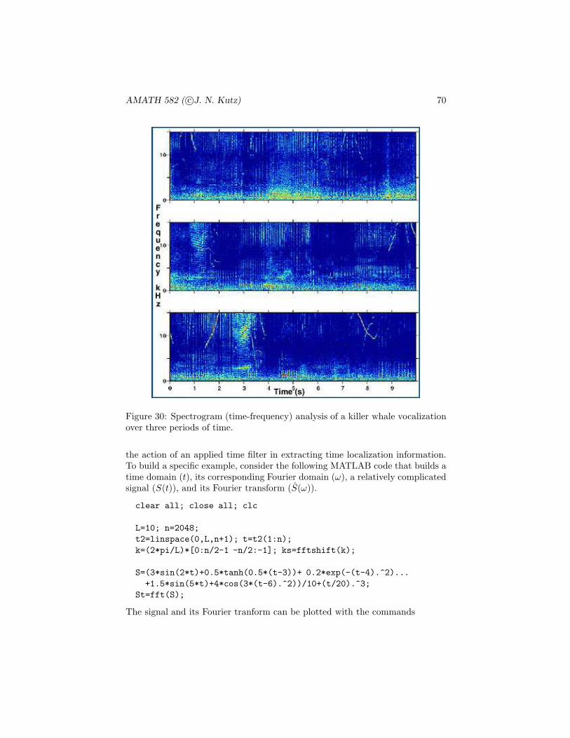
AMATH 582 ( c©J. N. Kutz) 70
Figure 30: Spectrogram (time-frequency) analysis of a killer whale vocalizationover three periods of time.
the action of an applied time filter in extracting time localization information.To build a specific example, consider the following MATLAB code that builds atime domain (t), its corresponding Fourier domain (ω), a relatively complicatedsignal (S(t)), and its Fourier transform (S(ω)).
clear all; close all; clc
L=10; n=2048;
t2=linspace(0,L,n+1); t=t2(1:n);
k=(2*pi/L)*[0:n/2-1 -n/2:-1]; ks=fftshift(k);
S=(3*sin(2*t)+0.5*tanh(0.5*(t-3))+ 0.2*exp(-(t-4).^2)...
+1.5*sin(5*t)+4*cos(3*(t-6).^2))/10+(t/20).^3;
St=fft(S);
The signal and its Fourier tranform can be plotted with the commands

AMATH 582 ( c©J. N. Kutz) 71
0 2 4 6 8 10−1
0
1
time (t)
S(t
)
−50 0 500
0.5
1
frequency (ω)
FF
T(S
)
Figure 31: Time signal and its Fourier transform considered for a time-frequencyanalysis in what follows.
figure(1)
subplot(3,1,1) % Time domain
plot(t,S,’k’)
set(gca,’Fontsize’,[14]),
xlabel(’Time (t)’), ylabel(’S(t)’)
subplot(3,1,2) % Fourier domain
plot(ks,abs(fftshift(St))/max(abs(St)),’k’);
axis([-50 50 0 1])
set(gca,’Fontsize’,[14])
xlabel(’frequency (\omega)’), ylabel(’FFT(S)’)
Figure 31 shows the signal and its Fourier transform for the above example.This signal S(t) will be analyzed using the Gabor transform method.
The simplest Gabor window to implement is a Gaussian time-filter centeredat some time τ with width a. As has been demonstrated, the parameter a iscritical for determining the level of time-resolution versus frequency resolutionin a time-frequency plot. Figure 32 shows the signal under consideration withthree filter widths. The more narrow the time-filtering, the better resolution intime. However, this also produces the worst resolution in frequency. Conversely,a wide window in time produces much better frequency resolution at the expenseof reducing the time resolution. A simple extension to the existing code producesa signal plot along with three different filter widths of Gaussian shape.
figure(2)
width=[10 1 0.2];
for j=1:3

AMATH 582 ( c©J. N. Kutz) 72
0 2 4 6 8 10−1
0
1
S(t
), g
(t)
0 2 4 6 8 10−1
0
1
S(t
), g
(t)
0 2 4 6 8 10−1
0
1
S(t
), g
(t)
time (t)
Figure 32: Time signal S(t) and the Gabor time filter g(t) (bold lines) for threedifferent Gaussian filters: g(t) = exp(−10(x − 4)2) (top), g(t) = exp(−(x −4)2) (middle), and g(t) = exp(−0.2(x − 4)2) (bottom). The different filterwidths determine the time-frequency resolution. Better time resolution givesworse frequency resolution and vice-versa due to the Heinsenberg uncertaintyprinciple.
g=exp(-width(j)*(t-4).^2);
subplot(3,1,j)
plot(t,S,’k’), hold on
plot(t,g,’k’,’Linewidth’,[2])
set(gca,’Fontsize’,[14])
ylabel(’S(t), g(t)’)
end
xlabel(’time (t)’)
The key now for the Gabor transform is to multiply the time filter Gaborfunction g(t) with the original signal S(t) in order to produce a windowed sectionof the signal. The Fourier transform of the windowed section then gives the localfrequency content in time. The following code constructs the windowed Fouriertransform with the Gabor filtering function
g(t) = e−a(t−b)2
. (2.7.54)

AMATH 582 ( c©J. N. Kutz) 73
0 2 4 6 8 10−1
0
1
S(t
), g
(t)
time (t)
0 2 4 6 8 10−1
0
1
S(t
)g(t
)
time (t)
−50 0 500
0.5
1
FF
T(S
g)
frequency (ω)
Figure 33: Time signal S(t) and the Gabor time filter g(t) = exp(−2(x − 4)2)(bold line) for a Gaussian filter. The product S(t)g(t) is depicted in the middlepanel and its Fourier transform Sg(ω) is depicted in the bottom panel. Notethat the windowing of the Fourier transform can severely limit the detection oflow-frequency components.
The Gaussian filtering has a width parameter a and translation parameter b.The following code constructs the windowed Fourier transform using the Gaus-sian with a = 2 and b = 4.
figure(3)
g=exp(-2*(t-4).^2);
Sg=g.*S;
Sgt=fft(Sg);
subplot(3,1,1), plot(t,S,’k’), hold on
plot(t,g,’k’,’Linewidth’,[2])
set(gca,’Fontsize’,[14])
ylabel(’S(t), g(t)’), xlabel(’time (t)’)
subplot(3,1,2), plot(t,Sg,’k’)
set(gca,’Fontsize’,[14])
ylabel(’S(t)g(t)’), xlabel(’time (t)’)
subplot(3,1,3), plot(ks,abs(fftshift(Sgt))/max(abs(Sgt)),’k’)
axis([-50 50 0 1])
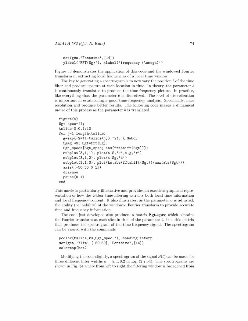
AMATH 582 ( c©J. N. Kutz) 74
set(gca,’Fontsize’,[14])
ylabel(’FFT(Sg)’), xlabel(’frequency (\omega)’)
Figure 33 demonstrates the application of this code and the windowed Fouriertransform in extracting local frequencies of a local time window.
The key to generating a spectrogram is to now vary the position b of the timefilter and produce spectra at each location in time. In theory, the parameter bis continuously translated to produce the time-frequency picture. In practice,like everything else, the parameter b is discretized. The level of discretizationis important in establishing a good time-frequency analysis. Specifically, finerresolution will produce better results. The following code makes a dynamicalmovie of this process as the parameter b is translated.
figure(4)
Sgt_spec=[];
tslide=0:0.1:10
for j=1:length(tslide)
g=exp(-2*(t-tslide(j)).^2); % Gabor
Sg=g.*S; Sgt=fft(Sg);
Sgt_spec=[Sgt_spec; abs(fftshift(Sgt))];
subplot(3,1,1), plot(t,S,’k’,t,g,’r’)
subplot(3,1,2), plot(t,Sg,’k’)
subplot(3,1,3), plot(ks,abs(fftshift(Sgt))/max(abs(Sgt)))
axis([-50 50 0 1])
drawnow
pause(0.1)
end
This movie is particularly illustrative and provides an excellent graphical repre-sentation of how the Gabor time-filtering extracts both local time informationand local frequency content. It also illustrates, as the parameter a is adjusted,the ability (or inability) of the windowed Fourier transform to provide accuratetime and frequency information.
The code just developed also produces a matrix Sgt spec which containsthe Fourier transform at each slice in time of the parameter b. It is this matrixthat produces the spectrogram of the time-frequency signal. The spectrogramcan be viewed with the commands
pcolor(tslide,ks,Sgt_spec.’), shading interp
set(gca,’Ylim’,[-50 50],’Fontsize’,[14])
colormap(hot)
Modifying the code slightly, a spectrogram of the signal S(t) can be made forthree different filter widths a = 5, 1, 0.2 in Eq. (2.7.54). The spectrograms areshown in Fig. 34 where from left to right the filtering window is broadened from

AMATH 582 ( c©J. N. Kutz) 75
Figure 34: Spectrograms produced from the Gabor time-filtering Eq. (2.7.54)with (a) a = 5, (b) a = 1 and (c) a = 0.2. The Fourier transform, which hasno time localization informatoin is depicted in (d). It is easily seen that thewindow width trades off time and frequency resolution at the expense of eachother. Regardless, the spectrogram gives a visual time-frequency picture of agiven signal.
a = 5 to a = 0.2. Note that for the left plot, strong localization of the signalin time is achieved at the expense of suppressing almost all the low-frequencycomponents of the signal. In contrast, the right most figure with a wide temporalfilter preserves excellent resolution of the Fourier domain but fails to localizesignals in time. Such are the tradeoffs associated with a fixed Gabor windowtransform.
2.8 MATLAB Filter Design and Wavelet Toolboxes
The applications of filtering and time-frequency analysis are so ubiquitous acrossthe sciences, that MATLAB has developed a suite of toolboxes that specialize inthese applications. Two of these toolboxes will be demonstrated in what follows.Primarily, screenshots will gives a hint of the functionality and versatility of thetoolboxes.
The most remarkable part of the toolboxes is that it allows for entry into high

AMATH 582 ( c©J. N. Kutz) 76
Figure 35: Screenshot of the filter design and analysis toolbox GUI. The topleft contains information on the current filter design while the top right is agraphical representation of the filter characteristics. The lower portion of theGUI is reserved for the user interface functionality and design. Indeed, the typeof filter, its spectral width, whether it is low-pass (filters high frequencies), high-pass (filters low frequencies), band-pass (filters a specified band of frequencies)or band-stop (attenuates a band of frequencies) can be chosen.
level signal processing and wavelet processing almost immediately. Indeed, onehardly needs to know anything to begin the process of analyzing, synthesizing,and manipulating data to one’s own ends. For the most part, each of thetoolboxes allows you to begin usage once you upload your signal, image or data.The only drawback is cost. For the most part, many academic departmentshave access to the toolboxes. And if you are part of a University environment,or enrolled in classes, the student versions of the toolboxes can be purchaseddirectly from MATLAB at a very reasonable price.

AMATH 582 ( c©J. N. Kutz) 77
Figure 36: Screenshot of the magnitude response of the filter. The magnituderesponse, along with a host of other important characteristics of the filter canbe obtained from the drag-down menu of the Analysis button on the top.
Filter Design and Analysis Toolbox
The filter design toolbox is ideally suited to help create and engineer and idealfilter for whatever application you may need. The user has the option of us-ing command line codes to directly access the filter design subroutines, or onecan use the extremely efficient and useful GUI (graphical user interface) fromMATLAB. Figure 35 shows a typical screenshot that MATLAB produces uponstartup of the filter design toolbox. The command to start the toolbox is givenby
FDAtool
This launches the highly intuitive GUI that guides you through the process ofdesigning your ideal filter. Figure 36 demonstrates, for instance, the magnituderesponse of the filter along with its frequency and magnitude of response. Themagnitude response can be accessed by dragging down the Analysis button atthe top of the GUI panel. In addition to the amplitude response, the phase

AMATH 582 ( c©J. N. Kutz) 78
response, a combination of phase and amplitude response, group-velocity re-sponse, etc. Depending upon your needs, complete engineering of the filter canbe performed with set objectives and performance aims.
As with all toolbox design and information, it can be exported from MAT-LAB for use in other programs or with other parts of MATLAB. The exportingof data, as well as saving of a given filter design, can all be performed from thefile drag-down menu at the top right of the GUI. Moreover, if you desire to skipthe filter design GUI, then all the filter functions can be accessed directly fromthe command line window. For instance, the command
[B,A]=butter(N,Wn)
generates a Butterworth digital and analog filter design. The parameter Ndenotes the Nth order lowpass digital Butterworth filter and returns the filtercoefficients in length N + 1 vectors B (numerator) and A (denominator). Thecoefficients are listed in descending powers of z. The cutoff frequency Wn mustbe 0.0 < Wn < 1.0, with 1.0 corresponding to half the sample rate. And besidesthis, you now know the butter command in MATLAB.
Wavelet Toolbox
Just like the signal processing, filter design toolbox, the wavelet toolbox itan immensely powerful toolbox for signal processing, image processing, multi-resolution analysis and any manner of time-frequency analysis. The wavelettoolbox is comprised of a large number of modules that allow for various appli-cations and methodologies. To access the toolbox, simply type
wavemenu
and a selection of menu items is generated. Figure 37 demonstrates the assort-ment of possible uses of the wavelet toolbox that are available upon launchingthe wavelet toolbox. In addition to such applications as signal processing andtime frequency analysis of one-dimensional signals or functions, one can proceedto denoise or manipulate image data. The program can also produce wavelettransforms and output the coefficients of a continuous or discrete wavelet trans-form.
As a specific example, consider the wavelet 1-D button and the examplefiles it contains. The example files are accessed from the file button at thetop left of the GUI. In this case, an example analysis of a noisy step functionsignal is considered. It should be noted that your own signal could have easilybeen imported from the file button with the load menu item. In this example,a signal is provided with the full wavelet decomposition at different levels ofresolution. It is easy to see that the given signal is decomposed into its bigfeatures followed by its finer features as one descends vertically down the plots.In the standard example, the sym wavelet is used with five levels of resolution.
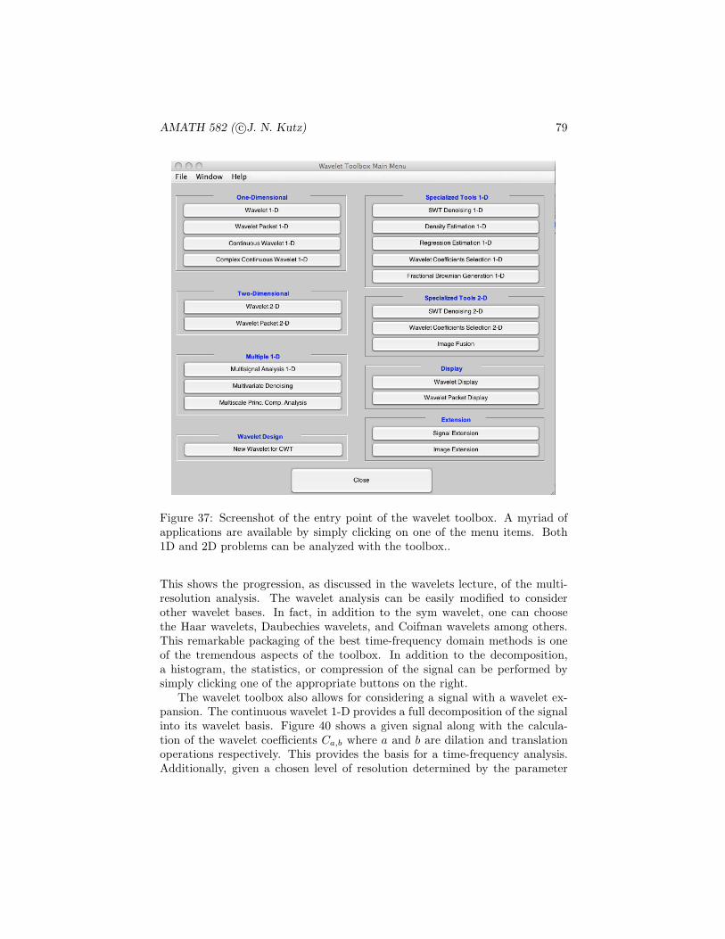
AMATH 582 ( c©J. N. Kutz) 79
Figure 37: Screenshot of the entry point of the wavelet toolbox. A myriad ofapplications are available by simply clicking on one of the menu items. Both1D and 2D problems can be analyzed with the toolbox..
This shows the progression, as discussed in the wavelets lecture, of the multi-resolution analysis. The wavelet analysis can be easily modified to considerother wavelet bases. In fact, in addition to the sym wavelet, one can choosethe Haar wavelets, Daubechies wavelets, and Coifman wavelets among others.This remarkable packaging of the best time-frequency domain methods is oneof the tremendous aspects of the toolbox. In addition to the decomposition,a histogram, the statistics, or compression of the signal can be performed bysimply clicking one of the appropriate buttons on the right.
The wavelet toolbox also allows for considering a signal with a wavelet ex-pansion. The continuous wavelet 1-D provides a full decomposition of the signalinto its wavelet basis. Figure 40 shows a given signal along with the calcula-tion of the wavelet coefficients Ca,b where a and b are dilation and translationoperations respectively. This provides the basis for a time-frequency analysis.Additionally, given a chosen level of resolution determined by the parameter
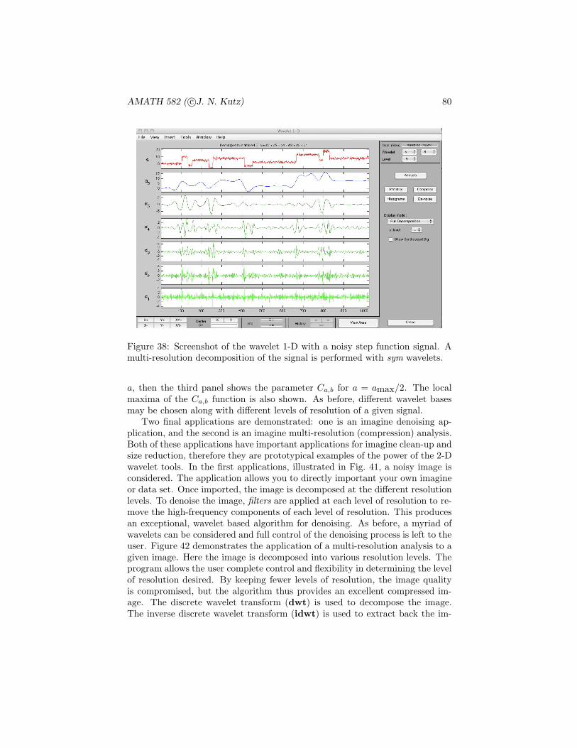
AMATH 582 ( c©J. N. Kutz) 80
Figure 38: Screenshot of the wavelet 1-D with a noisy step function signal. Amulti-resolution decomposition of the signal is performed with sym wavelets.
a, then the third panel shows the parameter Ca,b for a = amax/2. The localmaxima of the Ca,b function is also shown. As before, different wavelet basesmay be chosen along with different levels of resolution of a given signal.
Two final applications are demonstrated: one is an imagine denoising ap-plication, and the second is an imagine multi-resolution (compression) analysis.Both of these applications have important applications for imagine clean-up andsize reduction, therefore they are prototypical examples of the power of the 2-Dwavelet tools. In the first applications, illustrated in Fig. 41, a noisy image isconsidered. The application allows you to directly important your own imagineor data set. Once imported, the image is decomposed at the different resolutionlevels. To denoise the image, filters are applied at each level of resolution to re-move the high-frequency components of each level of resolution. This producesan exceptional, wavelet based algorithm for denoising. As before, a myriad ofwavelets can be considered and full control of the denoising process is left to theuser. Figure 42 demonstrates the application of a multi-resolution analysis to agiven image. Here the image is decomposed into various resolution levels. Theprogram allows the user complete control and flexibility in determining the levelof resolution desired. By keeping fewer levels of resolution, the image qualityis compromised, but the algorithm thus provides an excellent compressed im-age. The discrete wavelet transform (dwt) is used to decompose the image.The inverse discrete wavelet transform (idwt) is used to extract back the im-
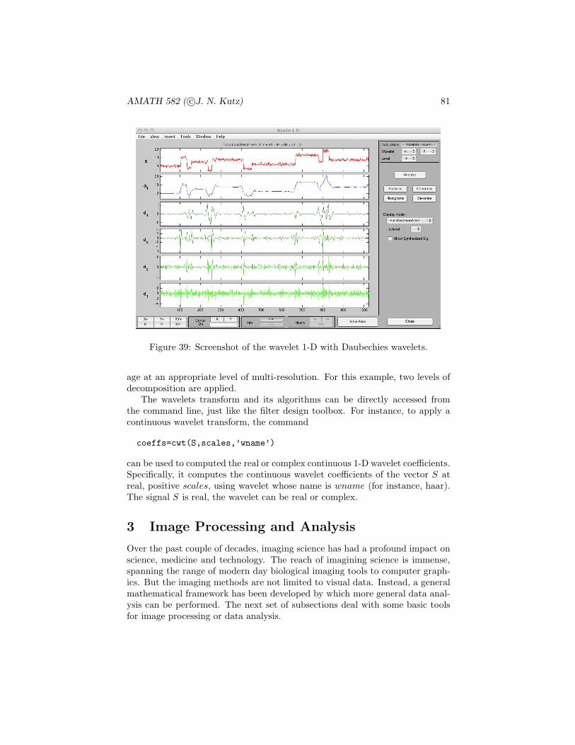
AMATH 582 ( c©J. N. Kutz) 81
Figure 39: Screenshot of the wavelet 1-D with Daubechies wavelets.
age at an appropriate level of multi-resolution. For this example, two levels ofdecomposition are applied.
The wavelets transform and its algorithms can be directly accessed fromthe command line, just like the filter design toolbox. For instance, to apply acontinuous wavelet transform, the command
coeffs=cwt(S,scales,’wname’)
can be used to computed the real or complex continuous 1-D wavelet coefficients.Specifically, it computes the continuous wavelet coefficients of the vector S atreal, positive scales, using wavelet whose name is wname (for instance, haar).The signal S is real, the wavelet can be real or complex.
3 Image Processing and Analysis
Over the past couple of decades, imaging science has had a profound impact onscience, medicine and technology. The reach of imagining science is immense,spanning the range of modern day biological imaging tools to computer graph-ics. But the imaging methods are not limited to visual data. Instead, a generalmathematical framework has been developed by which more general data anal-ysis can be performed. The next set of subsections deal with some basic toolsfor image processing or data analysis.
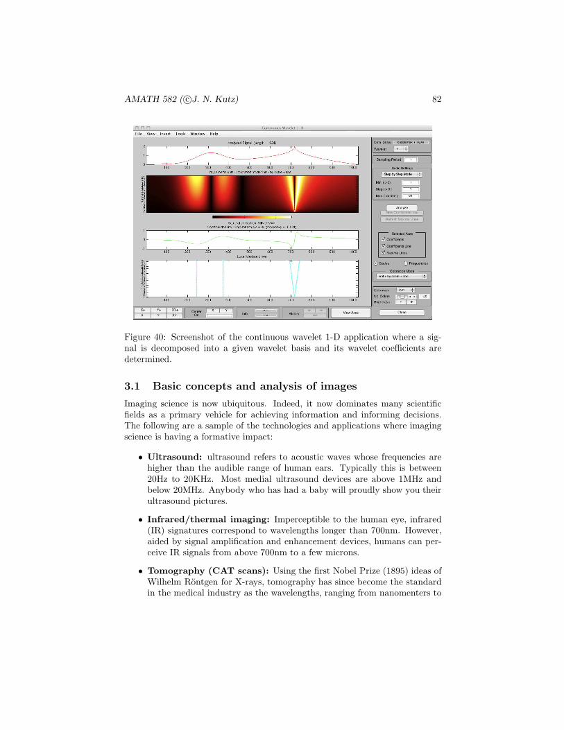
AMATH 582 ( c©J. N. Kutz) 82
Figure 40: Screenshot of the continuous wavelet 1-D application where a sig-nal is decomposed into a given wavelet basis and its wavelet coefficients aredetermined.
3.1 Basic concepts and analysis of images
Imaging science is now ubiquitous. Indeed, it now dominates many scientificfields as a primary vehicle for achieving information and informing decisions.The following are a sample of the technologies and applications where imagingscience is having a formative impact:
• Ultrasound: ultrasound refers to acoustic waves whose frequencies arehigher than the audible range of human ears. Typically this is between20Hz to 20KHz. Most medial ultrasound devices are above 1MHz andbelow 20MHz. Anybody who has had a baby will proudly show you theirultrasound pictures.
• Infrared/thermal imaging: Imperceptible to the human eye, infrared(IR) signatures correspond to wavelengths longer than 700nm. However,aided by signal amplification and enhancement devices, humans can per-ceive IR signals from above 700nm to a few microns.
• Tomography (CAT scans): Using the first Nobel Prize (1895) ideas ofWilhelm Rontgen for X-rays, tomography has since become the standardin the medical industry as the wavelengths, ranging from nanomenters to
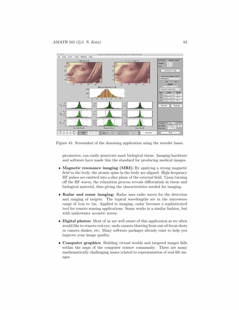
AMATH 582 ( c©J. N. Kutz) 83
Figure 41: Screenshot of the denoising application using the wavelet bases.
picometers, can easily penetrate most biological tissue. Imaging hardwareand software have made this the standard for producing medical images.
• Magnetic resonance imaging (MRI): By applying a strong magneticfield to the body, the atomic spins in the body are aligned. High-frequencyRF pulses are emitted into a slice plane of the external field. Upon turningoff the RF waves, the relaxation process reveals differentials in tissue andbiological material, thus giving the characteristics needed for imaging.
• Radar and sonar imaging: Radar uses radio waves for the detectionand ranging of targets. The typical wavelengths are in the microwaverange of 1cm to 1m. Applied to imaging, radar becomes a sophisticatedtool for remote sensing applications. Sonar works in a similar fashion, butwith underwater acoustic waves.
• Digital photos: Most of us are well aware of this application as we oftenwould like to remove red-eye, undo camera blurring from out-of-focus shotsor camera shakes, etc. Many software packages already exist to help youimprove your image quality.
• Computer graphics: Building virtual worlds and targeted images fallswithin the aegis of the computer science community. There are manymathematically challenging issues related to representation of real-life im-ages.
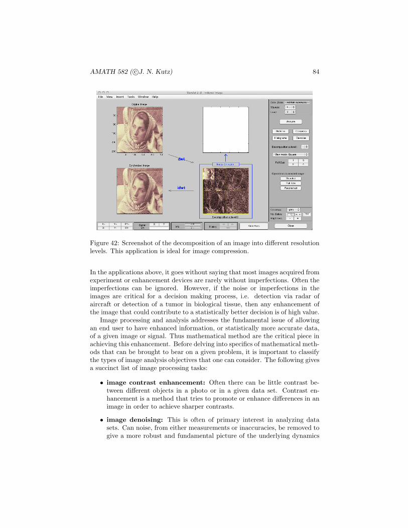
AMATH 582 ( c©J. N. Kutz) 84
Figure 42: Screenshot of the decomposition of an image into different resolutionlevels. This application is ideal for image compression.
In the applications above, it goes without saying that most images acquired fromexperiment or enhancement devices are rarely without imperfections. Often theimperfections can be ignored. However, if the noise or imperfections in theimages are critical for a decision making process, i.e. detection via radar ofaircraft or detection of a tumor in biological tissue, then any enhancement ofthe image that could contribute to a statistically better decision is of high value.
Image processing and analysis addresses the fundamental issue of allowingan end user to have enhanced information, or statistically more accurate data,of a given image or signal. Thus mathematical method are the critical piece inachieving this enhancement. Before delving into specifics of mathematical meth-ods that can be brought to bear on a given problem, it is important to classifythe types of image analysis objectives that one can consider. The following givesa succinct list of image processing tasks:
• image contrast enhancement: Often there can be little contrast be-tween different objects in a photo or in a given data set. Contrast en-hancement is a method that tries to promote or enhance differences in animage in order to achieve sharper contrasts.
• image denoising: This is often of primary interest in analyzing datasets. Can noise, from either measurements or inaccuracies, be removed togive a more robust and fundamental picture of the underlying dynamics

AMATH 582 ( c©J. N. Kutz) 85
of a system.
• image deblurring: The leading cause of bad pictures: camera shakes andout-of-focus cameras. Image processing methods can often compensateand undo these two phenomena to produce a sharper image that is greatlydeblurred. This is a remarkable application of image analysis, and isalready an application that is included in many digital photo softwarebundles.
• inpainting: If data is missing over certain portions of an image or setof data, inpainting provides a mathematical framework for systematicallygenerating the missing data. It accounts for both edges and the overallstructure surrounding the missing pixels.
• segmentation (edge detection): Segmentation breaks up an image intoblocks of different structures. This is particularly important for biomed-ical applications as well as military applications. Good algorithms fordetermining segmentation locations are critical.
The mathematical task is then to develop methods and algorithms capable ofperforming a set of tasks that addresses the above list. In the subsections thatfollow, only a small subset of these will be considered. However, a comprehensivemathematical treatment of the above issues can be performed [6].
Mathematical approaches
Given the broad appeal of imaging sciences and its applicability in such a widevariety of fields, it is not surprising that an equally diverse set of mathematicalmethods has been brought to bear on image processing. As with the previouslists of applications and tasks associated with image processing, the followinglist highlights some of the broad mathematical ideas that are present in thinkingabout image analysis.
Morphological approach: In this approach, one can think of the entire 2Ddomain of an image as a set of subdomains. Each subdomain should representsome aspect of the overall image. The fundamental idea here is to decomposethe domain into fundamental shapes based upon some structure element S. Thedomain is then decomposed in a binary way, a small patch of the image (definedby the structure element S) is in the object of interest or out of the object ofinterest. This provides an efficient method for edge detection in certain sets ofdata or images.
Fourier analysis: As with time-frequency analysis, the key idea is to de-compose the image into its Fourier components. This is easily done with a two-dimensional Fourier transform. Thus the image becomes a collection of Fourier
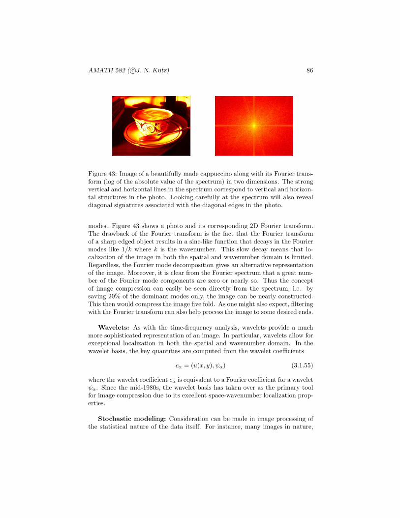
AMATH 582 ( c©J. N. Kutz) 86
Figure 43: Image of a beautifully made cappuccino along with its Fourier trans-form (log of the absolute value of the spectrum) in two dimensions. The strongvertical and horizontal lines in the spectrum correspond to vertical and horizon-tal structures in the photo. Looking carefully at the spectrum will also revealdiagonal signatures associated with the diagonal edges in the photo.
modes. Figure 43 shows a photo and its corresponding 2D Fourier transform.The drawback of the Fourier transform is the fact that the Fourier transformof a sharp edged object results in a sinc-like function that decays in the Fouriermodes like 1/k where k is the wavenumber. This slow decay means that lo-calization of the image in both the spatial and wavenumber domain is limited.Regardless, the Fourier mode decomposition gives an alternative representationof the image. Moreover, it is clear from the Fourier spectrum that a great num-ber of the Fourier mode components are zero or nearly so. Thus the conceptof image compression can easily be seen directly from the spectrum, i.e. bysaving 20% of the dominant modes only, the image can be nearly constructed.This then would compress the image five fold. As one might also expect, filteringwith the Fourier transform can also help process the image to some desired ends.
Wavelets: As with the time-frequency analysis, wavelets provide a muchmore sophisticated representation of an image. In particular, wavelets allow forexceptional localization in both the spatial and wavenumber domain. In thewavelet basis, the key quantities are computed from the wavelet coefficients
cα = (u(x, y), ψα) (3.1.55)
where the wavelet coefficient cα is equivalent to a Fourier coefficient for a waveletψα. Since the mid-1980s, the wavelet basis has taken over as the primary toolfor image compression due to its excellent space-wavenumber localization prop-erties.
Stochastic modeling: Consideration can be made in image processing ofthe statistical nature of the data itself. For instance, many images in nature,

AMATH 582 ( c©J. N. Kutz) 87
such as clouds, trees, sky, sandy beaches, are fundamentally statistical in nature.Thus one may not want to denoise such objects when performing image analysistasks. In the stochastic modeling approach, hidden features are explored withina given set of observed data which accounts for the statistical nature of manyof the underlying objects in an image.
Partial differential equations and diffusion: For denoising applications,or applications in which the data is choppy or highly pixelated, smoothing al-gorithms are of critical importance. In this case, one can take the original dataas the initial conditions of a diffusion process so that the image undergoes, inthe simplest case, the evolution
∂u
∂t= D∇2u (3.1.56)
where ∇2 = ∂2x + ∂2
y . This diffusion process provides smoothing to the originaldata file u. The key is knowing when the smoothing process should be stoppedso as not to remove too much image content.
Loading images, additive noise and MATLAB
To illustrate some of the various aspects of image processing, the following ex-ample will load the ideal image, apply Gaussian white noise to each pixel andshow the noisy image. In MATLAB, most standard image formats are easilyloaded. The key to performing mathematical manipulations is to then trans-form the data into double precision numbers which can be transformed, filtered,and manipulated at will. The generic data file uploaded in MATLAB is uint8which is an integer format ranging from 0 to 255. Moreover, color images havethree sets of data for each pixel in order to specific the RGB color coordinates.The following code uploads and image file (600x800 pixels). Although thereare 600x800 pixels, the data is stored as a 600x800x3 matrix where the extradimensions contain the color coding. This can be made into a 600x800 matrixby turning the image into a black-and-white picture. This is done in the codethat follows:
clear all; close all; clc;
A=imread(’photo’,’tiff’); % load image
Abw=rgb2gray(A); % make image black-and-white
subplot(2,2,1), image(A); set(gca,’Xtick’,[],’Ytick’,[])
subplot(2,2,3), imshow(Abw);
A2=double(A); % change form unit8 to double
Abw=double(Abw);
Note that at the end of the code, the matrices produced are converted to doubleprecision numbers.
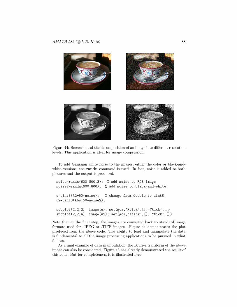
AMATH 582 ( c©J. N. Kutz) 88
Figure 44: Screenshot of the decomposition of an image into different resolutionlevels. This application is ideal for image compression.
To add Gaussian white noise to the images, either the color or black-and-white versions, the randn command is used. In fact, noise is added to bothpictures and the output is produced.
noise=randn(600,800,3); % add noise to RGB image
noise2=randn(600,800); % add noise to black-and-white
u=uint8(A2+50*noise); % change from double to uint8
u2=uint8(Abw+50*noise2);
subplot(2,2,2), image(u); set(gca,’Xtick’,[],’Ytick’,[])
subplot(2,2,4), image(u2); set(gca,’Xtick’,[],’Ytick’,[])
Note that at the final step, the images are converted back to standard imageformats used for .JPEG or .TIFF images. Figure 44 demonstrates the plotproduced from the above code. The ability to load and manipulate the datais fundamental to all the image processing applications to be pursued in whatfollows.
As a final example of data manipulation, the Fourier transform of the aboveimage can also be considered. Figure 43 has already demonstrated the result ofthis code. But for completeness, it is illustrated here

AMATH 582 ( c©J. N. Kutz) 89
Abw2=Abw(600:-1:1,:);
figure(2)
subplot(2,2,1), pcolor(Abw2), shading interp,
colormap(hot), set(gca,’Xtick’,[],’Ytick’,[])
Abwt=abs(fftshift(fft2(Abw2)));
subplot(2,2,2), pcolor(log(Abwt)), shading interp,
colormap(hot), set(gca,’Xtick’,[],’Ytick’,[])
Note that in this set of plots, we are once again working with matrices so thatcommands like pcolor are appropriate. These matrices are the subject of imageprocessing routines and algorithms.
3.2 Linear filtering for image denoising
As with time-frequency analysis and denoising of time signals, many applicationsof image processing deal with cleaning up images from imperfections, pixelation,and graininess, i.e. processing of noisy images. The objective in any imageprocessing application is to enhance or improve the quality of a given image.In this section, the filtering of noisy images will be considered with the aim ofproviding a higher quality, maximally denoised image.
The power of filtering has already been demonstrated in the context of radardetection applications. Ultimately, image denoising is directly related to filter-ing. To see this, consider Fig. 43 of the last section. In this image, the idealimage is represented along with the log of its Fourier transform. Like many im-ages, the Fourier spectrum is particularly sparse (or nearly zero) for most high-frequency components. Noise, however, tends to generate many high-frequencystructures on an image. Thus it is hoped that filtering of high-frequency com-ponents might remove unwanted noise fluctuations or graininess in an image.The top two panels of Fig. 45 show an initial noisy image and the log of itsFourier transform. These top two panels can be compared to the ideal imageand spectrum shown in Fig. 43. The code used to generate these top two panelsis given by the following:
A=imread(’photo’,’tiff’); Abw=rgb2gray(A);
Abw=double(Abw);
B=Abw+100*randn(600,800);
Bt=fft2(B); Bts=fftshift(Bt);
subplot(2,2,1), imshow(uint8(B)), colormap(gray)
subplot(2,2,2), pcolor((log(abs(Bts)))); shading interp
colormap(gray), set(gca,’Xtick’,[],’Ytick’,[])

AMATH 582 ( c©J. N. Kutz) 90
Figure 45: A noisy image and its Fourier transform are considered in the toppanel. The ideal image is shown in Fig. 43. By applying a linear Gaussian filter,the high-frequency noise components can be eliminated (bottom left) and theimage quality is significantly improved (bottom right).
Note that the uploaded image is converted to a double precision number throughthe double command. It can be transformed back to the image format via theuint8 command.
Linear filtering can be applied in the Fourier domain of the image in orderto remove the high-frequency scale fluctuations induced by the noise. A simplefilter to consider is a Gaussian that takes the form
F (kx, ky) = exp(−σx(kx − a)2 − σy(ky − b)2) (3.2.57)
where σx and σy are the filter widths in the x and y directions respectivelyand a and b are the center-frequency values for the corresponding filtering. Forthe image under consideration, it is a 600x800 pixel image so that the center-frequency components are located at kx = 301 and ky = 401 respectively. Tobuild a Gaussian filter, the following lines of code are needed:
kx=1:800; ky=1:600; [Kx,Ky]=meshgrid(kx,ky);
F=exp(-0.0001*(Kx-401).^2-0.0001*(Ky-301).^2);
Btsf=Bts.*F;
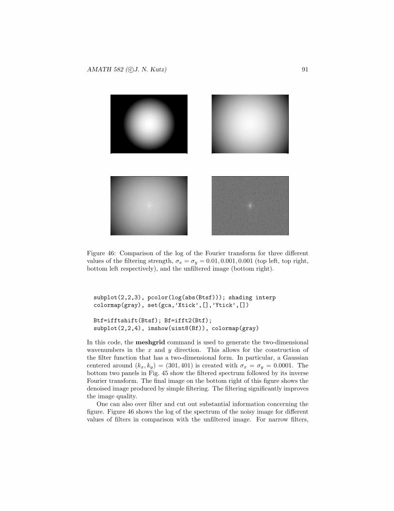
AMATH 582 ( c©J. N. Kutz) 91
Figure 46: Comparison of the log of the Fourier transform for three differentvalues of the filtering strength, σx = σy = 0.01, 0.001, 0.001 (top left, top right,bottom left respectively), and the unfiltered image (bottom right).
subplot(2,2,3), pcolor(log(abs(Btsf))); shading interp
colormap(gray), set(gca,’Xtick’,[],’Ytick’,[])
Btf=ifftshift(Btsf); Bf=ifft2(Btf);
subplot(2,2,4), imshow(uint8(Bf)), colormap(gray)
In this code, the meshgrid command is used to generate the two-dimensionalwavenumbers in the x and y direction. This allows for the construction ofthe filter function that has a two-dimensional form. In particular, a Gaussiancentered around (kx, ky) = (301, 401) is created with σx = σy = 0.0001. Thebottom two panels in Fig. 45 show the filtered spectrum followed by its inverseFourier transform. The final image on the bottom right of this figure shows thedenoised image produced by simple filtering. The filtering significantly improvesthe image quality.
One can also over filter and cut out substantial information concerning thefigure. Figure 46 shows the log of the spectrum of the noisy image for differentvalues of filters in comparison with the unfiltered image. For narrow filters,

AMATH 582 ( c©J. N. Kutz) 92
Figure 47: Comparison of the image quality for the three filter strengths con-sidered in Fig. 46. A high degree of filtering blurs the image and no fine scalefeatures are observed (top right). In contrast, moderate strength filtering pro-duces exceptional improvement of the image quality (top right and bottom left).These denoised images should be compared to the unfiltered image (bottomright).
much of the image information is irretrievably lost along with the noise. Findingan optimal filter is part of the image processing agenda. In the image spatialdomain, the filtering strength (or width) can be considered. Figure 47 shows aseries of filtered images and their comparison to the unfiltered image. Strongfiltering produces a smooth, yet blurry image. In this case, all fine scale featuresare lost. Moderate levels of filtering produce reasonable images with significantreduction of the noise in comparison to the non-filtered image. The followingcode was used to produce these last two figures.
% Gaussian filter
fs=[0.01 0.001 0.0001 0];
for j=1:4
F=exp(-fs(j)*(Kx-401).^2-fs(j)*(Ky-301).^2);
Btsf=Bts.*F; Btf=ifftshift(Btsf); Bf=ifft2(Btf);
figure(4), subplot(2,2,j), pcolor(log(abs(Btsf)))
shading interp,colormap(gray),set(gca,’Xtick’,[],’Ytick’,[])

AMATH 582 ( c©J. N. Kutz) 93
Figure 48: A noisy image and its Fourier transform are considered in the toppanel. The ideal image is shown in Fig. 43. By applying a Shannon (stepfunction) filter, the high-frequency noise components can be eliminated (bottomleft) and the image quality is significantly improved (bottom right).
figure(5), subplot(2,2,j), imshow(uint8(Bf)), colormap(gray)
end
Note that the processed data is converted back to a graphics image beforeplotting with the imshow command.
Gaussian filtering is only one type of filtering that can be applied. Thereare, just like in signal processing applications, myriads of filters that can beused to process a given image, including low-pass, high-pass, band-pass, etc. Asa second example filter, the Shannon filter is considered. The Shannon filter issimply a step function with value of unity within the transmitted band and zerooutside of it. In the example that follows, a Shannon filter is applied of width50 pixels around the center frequency of the image.
width=50;
Fs=zeros(600,800);
Fs(301-width:1:301+width,401-width:1:401+width) ...
=ones(1:2*width+1,1:2*width+1);
Btsf=Bts.*Fs;

AMATH 582 ( c©J. N. Kutz) 94
Figure 49: Comparison of the image quality for the three filter widths. A highdegree of filtering blurs the image and no fine scale features are observed (topright). In contrast, moderate strength filtering produces exceptional improve-ment of the image quality (top right and bottom left). These denoised imagesshould be compared to the unfiltered image (bottom right).
Btf=ifftshift(Btsf); Bf=ifft2(Btf);
subplot(2,2,3), pcolor(log(abs(Btsf))); shading interp
colormap(gray), set(gca,’Xtick’,[],’Ytick’,[])
subplot(2,2,4), imshow(uint8(Bf)), colormap(gray)
Figure 48 is a companion figure to Fig. 45. The only difference between themis the filter chosen for the image processing. The key difference is representedin the lower left panel of both figures. Note that the Shannon filter simplysuppresses all frequencies outside of a given filter box. The performance dif-ference between Gaussian filtering and Shannon filtering appears to be fairlymarginal. However, there may be some applications where one or the other ismore suitable. The image enhancement can also be explored as a function of theShannon filter width. Figure 49 shows the image quality as the filter is widenedalong with the unfiltered image. Strong filtering again produces a blurred imagewhile moderate filtering produces a greatly enhanced image quality. A code to

AMATH 582 ( c©J. N. Kutz) 95
produce this image is given by the following:
fs=[10 50 100 200];
for j=1:4
Fs=zeros(600,800);
Fs(301-fs(j):1:301+fs(j),401-fs(j):1:401+fs(j)) ...
=ones(1:2*fs(j)+1,1:2*fs(j)+1);
Btsf=Bts.*Fs; Btf=ifftshift(Btsf); Bf=ifft2(Btf);
figure(7), subplot(2,2,j), imshow(uint8(Bf)), colormap(gray)
end
The width is adjusted by considering the number of filter pixels around thecenter frequency with value unity. One might be able to argue that the Gaussianfilter produces slightly better image results since the inverse Fourier transformof a step function filter produces sinc-like behavior.
3.3 Diffusion and image processing
Filtering is not the only way to denoise an image. Intimately related to filteringis the use of diffusion for image enhancement. Consider for the moment thesimplest spatial diffusion process in two dimensions, i.e. the heat equation:
ut = D∇2u (3.3.58)
where u(x, y) will represent a given image, ∇2 = ∂2x + ∂2
y , D is a diffusioncoefficient, and some boundary conditions must be imposed. If for the momentwe consider periodic boundary conditions, then the solution to the heat equationcan be found from, for instance, the Fourier transform
ut = −D(k2x + k2
y)u → u = u0e−D(k2
x+k2
y)t (3.3.59)
where the u is the Fourier transform of u(x, y) and u0 is the Fourier transformof the initial conditions, i.e. the original noisy image. The solution of theheat equation illustrates a key and critical concept: the wavenumbers (spatialfrequencies) decay according to a Gaussian function. Thus linear filtering witha Gaussian is equivalent to a linear diffusion of the image for periodic boundaryconditions.
The above argument establishes some equivalency between filtering and dif-fusion. However, the diffusion formalism provides a more general framework inwhich to consider image cleanup since the heat equation can be modified to
ut = ∇ · (D(x, y)∇u) (3.3.60)
where D(x, y) is now a spatial diffusion coefficient. In particular, the diffusioncoefficient could be used to great advantage to target trouble spots on an imagewhile leaving relatively noise free patches alone.

AMATH 582 ( c©J. N. Kutz) 96
To solve the heat equation numerically, we discretize the spatial derivativewith a second-order scheme (see Table ??) so that
∂2u
∂x2=
1
∆x2[u(x+ ∆x, y) − 2u(x, y) + u(x− ∆x, y)] (3.3.61a)
∂2u
∂y2=
1
∆y2[u(x, y + ∆y) − 2u(x, y) + u(x, y − ∆y)] . (3.3.61b)
This approximation reduces the partial differential equation to a system of ordi-nary differential equations. Once this is accomplished, then a variety of standardtime-stepping schemes for differential equations can be applied to the resultingsystem.
The ODE system for 1D diffusion
Consider first diffusion in one-dimension so that u(x, y) = u(x). The vectorsystem for MATLAB can then be formulated. To define the system of ODEs,we discretize and define the values of the vector u in the following way.
u(−L) = u1
u(−L+ ∆x) = u2
...
u(L− 2∆x) = un−1
u(L− ∆x) = un
u(L) = un+1 .
If periodic boundary conditions, for instance, are considered, then periodicityrequires that u1 = un+1. Thus the system of differential equations solves forthe vector
u =
u1
u2
...un
. (3.3.62)
The governing heat equation is then reformulated in discretized form as thedifferential equations system
du
dt=
κ
∆x2Au , (3.3.63)
AMATH 582 ( c©J. N. Kutz) 97
where A is given by the sparse matrix
A=
−2 1 0 · · · 0 11 −2 1 0 · · · 0
0. . .
. . .. . .
......0
... · · · 0 1 −2 11 0 · · · 0 1 −2
, (3.3.64)
and the values of one on the upper right and lower left of the matrix result fromthe periodic boundary conditions.
MATLAB implementation
The system of differential equations can now be easily solved with a standardtime-stepping algorithm such as ode23 or ode45. The basic algorithm would beas follows
1. Build the sparse matrix A.
e1=ones(n,1); % build a vector of ones
A=spdiags([e1 -2*e1 e1],[-1 0 1],n,n); % diagonals
A(1,n)=1; A(n,1)=1; % periodic boundaries
2. Generate the desired initial condition vector u = u0.
3. Call an ODE solver from the MATLAB suite. The matrix A, the diffusionconstant κ and spatial step ∆x need to be passed into this routine.
[t,y]=ode45(’rhs’,tspan,u0,[],k,dx,A);
The function rhs.m should be of the following form
function rhs=rhs(tspan,u,dummy,k,dx,A)
rhs=(k/dx^2)*A*u;
4. Plot the results as a function of time and space.
The algorithm is thus fairly routine and requires very little effort in programmingsince we can make use of the standard time-stepping algorithms already availablein MATLAB.
AMATH 582 ( c©J. N. Kutz) 98
2D MATLAB implementation
In the case of two dimensions, the calculation becomes slightly more difficultsince the 2D data is represented by a matrix and the ODE solvers require avector input for the initial data. For this case, the governing equation is
∂u
∂t= κ
(∂2u
∂x2+∂2u
∂y2
)(3.3.65)
Provided ∆x = ∆y = δ are the same, the system can be reduced to the linearsystem
du
dt=
κ
δ2Au , (3.3.66)
where we have arranged the vector u by stacking slices of the data in the seconddimension y. This stacking procedure is required for implementation purposesof MATLAB. Thus be defining
unm = u(xn, ym) (3.3.67)
the collection of image (pixel) points can be arranged as follows
u =
u11
u12
...u1n
u21
u22
...un(n−1)
unn
, (3.3.68)
The matrix A is a sparse matrix and so the sparse implementation of this matrixcan be be used advantageously in MATLAB.
Again, the system of differential equations can now be easily solved with astandard time-stepping algorithm such as ode23 or ode45. The basic algorithmfollows the same course as the 1D case, but extra care is taken in arranging the2D data into a vector.
subsubsection*Diffusion of an imageTo provide a basic implementation of the above methods, consider the fol-
lowing MATLAB code which loads a given image file, converts it to doubleprecision numbers, then diffuses the image in order to remove some of the noisecontent. The process begins once again with the loading of an ideal image onwhich noise will be projected.
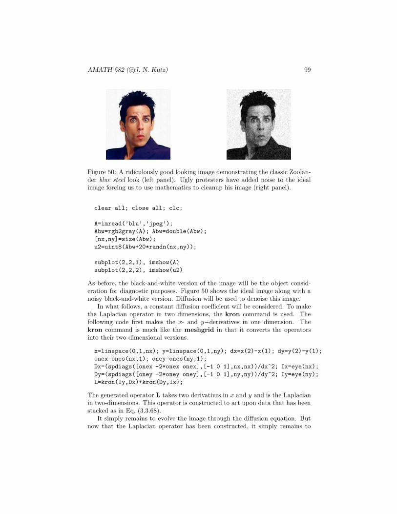
AMATH 582 ( c©J. N. Kutz) 99
Figure 50: A ridiculously good looking image demonstrating the classic Zoolan-der blue steel look (left panel). Ugly protesters have added noise to the idealimage forcing us to use mathematics to cleanup his image (right panel).
clear all; close all; clc;
A=imread(’blu’,’jpeg’);
Abw=rgb2gray(A); Abw=double(Abw);
[nx,ny]=size(Abw);
u2=uint8(Abw+20*randn(nx,ny));
subplot(2,2,1), imshow(A)
subplot(2,2,2), imshow(u2)
As before, the black-and-white version of the image will be the object consid-eration for diagnostic purposes. Figure 50 shows the ideal image along with anoisy black-and-white version. Diffusion will be used to denoise this image.
In what follows, a constant diffusion coefficient will be considered. To makethe Laplacian operator in two dimensions, the kron command is used. Thefollowing code first makes the x- and y−derivatives in one dimension. Thekron command is much like the meshgrid in that it converts the operatorsinto their two-dimensional versions.
x=linspace(0,1,nx); y=linspace(0,1,ny); dx=x(2)-x(1); dy=y(2)-y(1);
onex=ones(nx,1); oney=ones(ny,1);
Dx=(spdiags([onex -2*onex onex],[-1 0 1],nx,nx))/dx^2; Ix=eye(nx);
Dy=(spdiags([oney -2*oney oney],[-1 0 1],ny,ny))/dy^2; Iy=eye(ny);
L=kron(Iy,Dx)+kron(Dy,Ix);
The generated operator L takes two derivatives in x and y and is the Laplacianin two-dimensions. This operator is constructed to act upon data that has beenstacked as in Eq. (3.3.68).
It simply remains to evolve the image through the diffusion equation. Butnow that the Laplacian operator has been constructed, it simply remains to

AMATH 582 ( c©J. N. Kutz) 100
Figure 51: Image denoising process for a diffusion constant of D = 0.0005 asa function of time for t = 0, 0.004, 0.008 and 0.016. Perhaps the best image isfor t = 0.008 where a moderate amount of diffusion has been applied. Furtherdiffusion starts to degrade the image quality.
reshape the image, determine a time-span for evolving, and choose a diffusioncoefficient. The following code performs the diffusion of the image and producesa plot that tracks the image from its initial state to the final diffused image.
tspan=[0 0.004 0.008 0.016]; D=0.0005;
u3=Abw+20*noise2;
u3_2=reshape(u3,nx*ny,1);
[t,usol]=ode113(’image_rhs’,tspan,u3_2,[],L,D);
for j=1:length(t)
Abw_clean=uint8(reshape(usol(j,:),nx,ny));
subplot(2,2,j), imshow(Abw_clean);
end
The above code calls on the function image rhs which contains the diffusionequation information. This function contains the following two lines of code:
function rhs=image_rhs(t,u,dummy,L,D)
rhs=D*L*u;
AMATH 582 ( c©J. N. Kutz) 101
Figure 51 shows the evolution of the image through the diffusion process. Notethat only a slight amount of diffusion is needed, i.e. a small diffusion constantas well as a short diffusion time, before the pixelation has been substantiallyreduced. Continued diffusion starts to degrade image quality. This correspondsto over-filtering the image.
Nonlinear filtering and diffusion
As mentioned previously, the linear diffusion process is equivalent to the appli-cation of a Gaussian filter. Thus it is not clear that the diffusion process is anybetter than simple filtering. However, the diffusion process has several distinctadvantages: first, particular regions in the spatial figure can be targeted bymodification of the diffusion coefficient D(x, y). Second, nonlinear diffusion canbe considered for enhancing certain features of the image. This corresponds toa nonlinear filtering process. In this case,
ut = ∇ · (D(u,∇u)∇u) (3.3.69)
where the diffusion coefficient now depends on the image and its gradient. Non-linear diffusion, with a properly constructed D above, can be used, for instance,as an effective method for extracting edges from an image [6]. Thus althoughthis section has only considered a simple linear diffusion model, the ideas areeasily generalized to account for more general concepts and image processingaims.
4 Linear Algebra and Singular Value Decompo-sition
Linear algebra plays a central role in almost every application area of math-ematics in the physical, engineering and biological sciences. It is perhaps themost important theoretical framework to be familiar with as a student of math-ematics. Thus it is no surprise that it also plays a key role in data analysis andcomputation. In what follows, emphasis will placed squarely on the singularvalue decomposition (SVD). This concept is often untouched in undergraduatecourses in linear algebra, yet it forms one of the most powerful techniques foranalyzing a myriad of applications areas.
4.1 Basics of The Singular Value Decomposition (SVD)
In even the earliest experience of linear algebra, the concept of a matrix trans-forming a vector via multiplication was defined. For instance, the vector x whenmultiplied by a matrix A produces a new vector y that is now aligned, generi-cally, in a new direction with a new length. To be more specific, the following
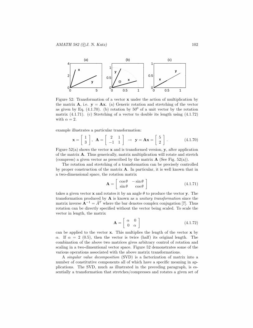
AMATH 582 ( c©J. N. Kutz) 102
0 50
2
4
y
x
(a)
0 0.5 10
0.5
1
Θ x
y
(b)
0 0.5 10
0.5
1
x
y
(c)
Figure 52: Transformation of a vector x under the action of multiplication bythe matrix A, i.e. y = Ax. (a) Generic rotation and stretching of the vectoras given by Eq. (4.1.70). (b) rotation by 500 of a unit vector by the rotationmatrix (4.1.71). (c) Stretching of a vector to double its length using (4.1.72)with α = 2.
example illustrates a particular transformation:
x =
[13
], A =
[2 1−1 1
]→ y = Ax =
[52
]. (4.1.70)
Figure 52(a) shows the vector x and is transformed version, y, after applicationof the matrix A. Thus generically, matrix multiplication will rotate and stretch(compress) a given vector as prescribed by the matrix A (See Fig. 52(a)).
The rotation and stretching of a transformation can be precisely controlledby proper construction of the matrix A. In particular, it is well known that ina two-dimensional space, the rotation matrix
A =
[cos θ − sin θsin θ cos θ
](4.1.71)
takes a given vector x and rotates it by an angle θ to produce the vector y. Thetransformation produced by A is known as a unitary transformation since thematrix inverse A−1 = AT where the bar denotes complex conjugation [7]. Thusrotation can be directly specified without the vector being scaled. To scale thevector in length, the matrix
A =
[α 00 α
](4.1.72)
can be applied to the vector x. This multiplies the length of the vector x byα. If α = 2 (0.5), then the vector is twice (half) its original length. Thecombination of the above two matrices gives arbitrary control of rotation andscaling in a two-dimentional vector space. Figure 52 demonstrates some of thevarious operations associated with the above matrix transformations.
A singular value decomposition (SVD) is a factorization of matrix into anumber of constitutive components all of which have a specific meaning in ap-plications. The SVD, much as illustrated in the preceding paragraph, is es-sentially a transformation that stretches/compresses and rotates a given set of

AMATH 582 ( c©J. N. Kutz) 103
v1
v2
S
σ1 u
1
σ2 u
2
A
AS
Figure 53: Image of a unit sphere S transformed into a hyperellipse AS in R2.The values of σ1 and σ2 are the singular values of the matrix A and representthe lengths of the semiaxes of the ellipse.
vectors. In particular, the following geometric principle will guide our forth-coming discussion: the image of a unit sphere under any m × n matrix is ahyperellipse. A hyperellipse in Rm is defined by the surface obtained uponstretching a unit sphere in Rm by some factors σ1, σ2, · · · , σm in the orthogo-nal directions u1,u2, · · · ,um ∈ Rm. The stretchings σi can possibly be zero.For convenience, consider the uj to be unit vectors so that ‖uj‖2 = 1. Thequantity σjuj is then the principal semiaxes of the hyperellipse with the lengthσj . Figure 53 demonstrates a particular hyperellipse created under the matrixtransformation A in R2.
A few things are worth noting at this point. First, if A has rank r, exactlyr of the lengths σj will be nonzero. And if the matrix A is an m × n matrixwhere m > n, at most n of the σj will be nonzero. Consider for the momenta full rank matrix A. Then the n singular values of A are the lengths ofthe principal semiaxes AS as shown in Fig. 53. Convention assumes that thesingular values are ordered with the largest first and then in descending order:σ1 ≥ σ2 ≥ · · · ≥ σn > 0.
On a more formal level, the transformation from the unit sphere to thehyperellipse can be more succinctly stated as follows:
Avj = σjuj 1 ≤ j ≤ n . (4.1.73)
Thus in total, there are n vectors that are transformed under A. A more com-
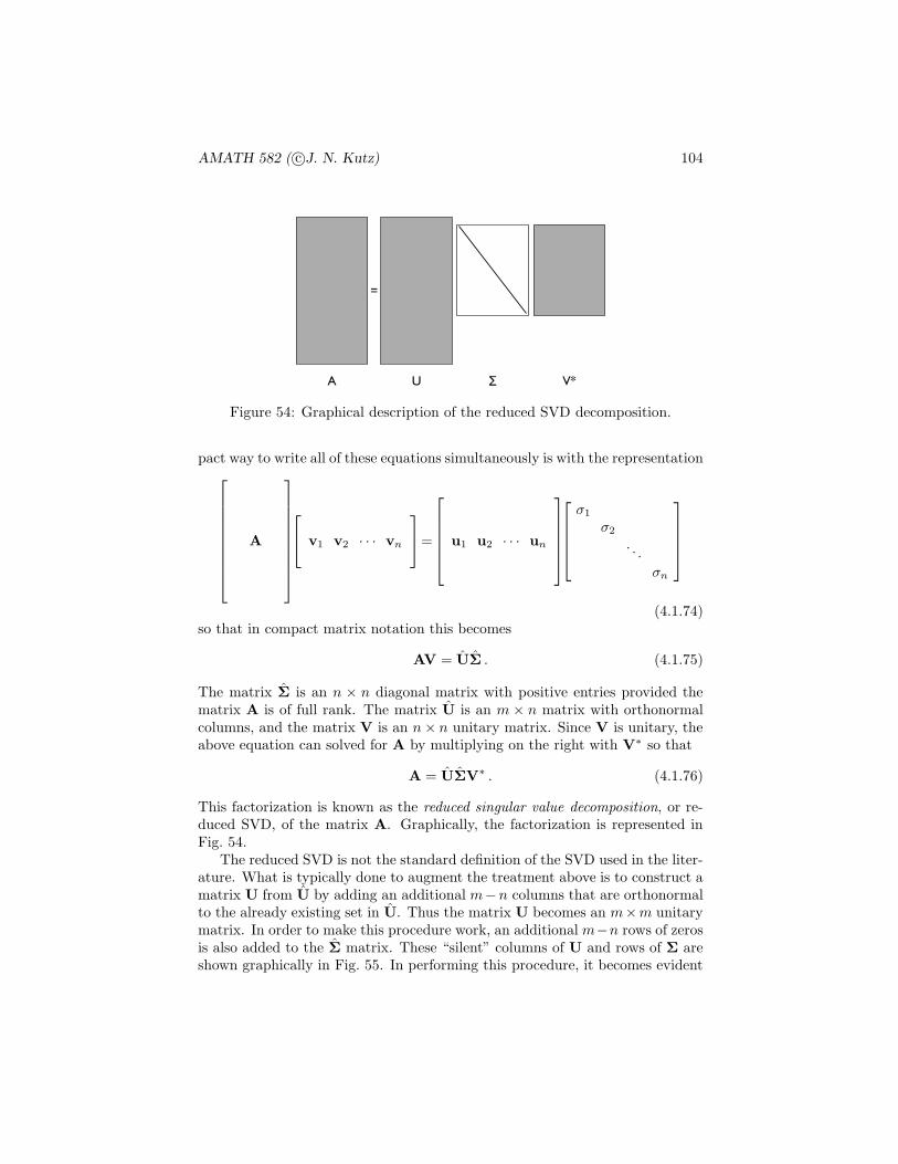
AMATH 582 ( c©J. N. Kutz) 104
A ! V*U
=
Figure 54: Graphical description of the reduced SVD decomposition.
pact way to write all of these equations simultaneously is with the representation
A
v1 v2 · · · vn
=
u1 u2 · · · un
σ1
σ2
. . .
σn
(4.1.74)so that in compact matrix notation this becomes
AV = UΣ . (4.1.75)
The matrix Σ is an n × n diagonal matrix with positive entries provided thematrix A is of full rank. The matrix U is an m × n matrix with orthonormalcolumns, and the matrix V is an n× n unitary matrix. Since V is unitary, theabove equation can solved for A by multiplying on the right with V∗ so that
A = UΣV∗ . (4.1.76)
This factorization is known as the reduced singular value decomposition, or re-duced SVD, of the matrix A. Graphically, the factorization is represented inFig. 54.
The reduced SVD is not the standard definition of the SVD used in the liter-ature. What is typically done to augment the treatment above is to construct amatrix U from U by adding an additional m−n columns that are orthonormalto the already existing set in U. Thus the matrix U becomes an m×m unitarymatrix. In order to make this procedure work, an additional m−n rows of zerosis also added to the Σ matrix. These “silent” columns of U and rows of Σ areshown graphically in Fig. 55. In performing this procedure, it becomes evident
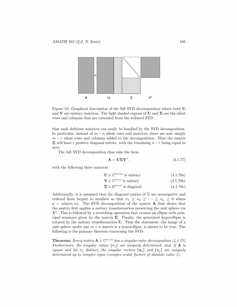
AMATH 582 ( c©J. N. Kutz) 105
A ! V*U
=
Figure 55: Graphical description of the full SVD decomposition where both Uand V are unitary matrices. The light shaded regions of U and Σ are the silentrows and columns that are extended from the reduced SVD.
that rank deficient matrices can easily be handled by the SVD decomposition.In particular, instead of m − n silent rows and matrices, there are now simplym − r silent rows and columns added to the decomposition. Thus the matrixΣ will have r positive diagonal entries, with the remaining n− r being equal tozero.
The full SVD decomposition thus take the form
A = UΣV∗ . (4.1.77)
with the following three matrices
U ∈ Cm×m is unitary (4.1.78a)
V ∈ Cn×n is unitary (4.1.78b)
Σ ∈ Rm×n is diagonal (4.1.78c)
Additionally, it is assumed that the diagonal entries of Σ are nonnegative andordered from largest to smallest so that σ1 ≥ σ2 ≥ · · · ≥ σp ≥ 0 wherep = min(m,n). The SVD decomposition of the matrix A thus shows thatthe matrix first applies a unitary transformation preserving the unit sphere viaV∗. This is followed by a stretching operation that creates an ellipse with prin-cipal semiaxes given by the matrix Σ. Finally, the generated hyperellipse isrotated by the unitary transformation U. Thus the statement: the image of aunit sphere under any m× n matrix is a hyperellipse, is shown to be true. Thefollowing is the primary theorem concerning the SVD:
Theorem: Every matrix A ∈ Cm×n has a singular value decomposition (4.1.77).Furthermore, the singular values {σj} are uniquely determined, and, if A issquare and the σj distinct, the singular vectors {uj} and {vj} are uniquelydetermined up to complex signs (complex scalar factors of absolute value 1).

AMATH 582 ( c©J. N. Kutz) 106
Computing the SVD
The above theorem guarantees the existence of the SVD, but in practice, it stillremains to be computed. This is a fairly straightforward process if one considersthe following matrix products:
ATA = (UΣV∗)T (UΣV∗)
= VΣU∗UΣV∗
= VΣ2V∗ (4.1.79)
and
AAT = (UΣV∗)(UΣV∗)T
= UΣV∗VΣU∗
= UΣ2U∗ . (4.1.80)
Multiplying (4.1.79) and (4.1.80) on the right by V and U respectively givesthe two self-consistent eigenvalue problems
ATAV = VΣ2 (4.1.81a)
AATU = UΣ2 . (4.1.81b)
Thus if the normalized eigenvectors are found for these two equations, then theorthonormal basis vectors are produced for U and V. Likewise, the square rootof the eigenvalues of these equations produces the singular values σj .
Example: Consider the SVD decomposition of
A =
[3 00 −2
]. (4.1.82)
The following quantities are computed:
ATA =
[3 00 −2
] [3 00 −2
]=
[9 00 4
](4.1.83a)
AAT =
[3 00 −2
] [3 00 −2
]=
[9 00 4
]. (4.1.83b)
The eigenvalues are clearly λ = {9, 4}, giving singular values σ1 = 3 and σ2 = 2.The eigenvectors can similarly be constructed and the matrices U and V aregiven by [
±1 00 ±1
](4.1.84)
where there is an indeterminate sign in the eigenvectors. However, a self-consistent choice of signs must be made. One possible choice gives
A = UΣV∗ =
[1 00 1
] [3 00 2
] [1 00 −1
](4.1.85)
AMATH 582 ( c©J. N. Kutz) 107
The SVD can be easily computed in MATLAB with the following command:
[U,S,V]=svd(A);
where the [U, V,D] correspond to U, Σ and V respectively. This decomposi-tion is a critical tool for analyzing many data driven phenomena. But beforeproceeding to such applications, the connection of the SVD with standard andwell-known techniques is elucidated.
4.2 The SVD in broader context
The SVD is an exceptionally important tool in many areas of applications.Part of this is due to its many mathematical properties and its guarantee ofexistence. In what follows, some of its more important theorems and relationsto other standard ideas of linear algebra are considered with the aim of settingthe mathematical framework for future applications.
Eigenvalues, eigenvectors and diagonalization
The concept of eigenvalues and eigenvectors is critical to understanding manyareas of applications. One of the most important areas where it plays a role isin understanding differential equations. Consider, for instance, the system ofdifferential equations:
dy
dt= Ay (4.2.86)
for some vector y(t) representing a dynamical system of variables and wherethe matrix A determines the interaction among these variables. Assuming asolution of the form y = x exp(λt) results in the eigenvalue problem:
Ax = λx . (4.2.87)
The questions remains: how are the eigenvalues and eigenvectors found? Toconsider this problem, we rewrite the eigenvalue problem as
Ax − λIx = (A − λI)x = 0. (4.2.88)
Two possibilities now exist.
Option I: The determinant of the matrix (A−λI) is not zero. If this is true, thematrix is nonsingular and its inverse, (A − λI)−1, can be found. The solutionto the eigenvalue problem (4.2.87) is then
x = (A − λI)−10 (4.2.89)
which implies that x = 0. This trivial solution could have easily been guessed.However, it is not relevant as we require nontrivial solutions for x.
AMATH 582 ( c©J. N. Kutz) 108
Option II: The determinant of the matrix (A− λI) is zero. If this is true, thematrix is singular and its inverse, (A−λI)−1, cannot be found. Although thereis no longer a guarantee that there is a solution, it is the only scenario whichallows for the possibility of x 6= 0. It is this condition which allows for theconstruction of eigenvalues and eigenvectors. Indeed, we choose the eigenvaluesλ so that this condition holds and the matrix is singular.
Another important operation which can be performed with eigenvalue andeigenvectors is the evaluation of
AM (4.2.90)
where M is a large integer. For large matrices A, this operation is computa-tionally expensive. However, knowing the eigenvalues and eigenvectors of Aallows for a significant ease in computational expense. Assuming we have allthe eigenvalues and eigenvectors of A, then
Ax1 = λ1x1
Ax2 = λ2x2
...
Axn = λ1xn .
This collection of eigenvalues and eigenvectors gives the matrix system
AS = SΛ (4.2.91)
where the columns of the matrix S are the eigenvectors of A,
S = (x1 x2 · · · xn) , (4.2.92)
and Λ is a matrix whose diagonals are the corresponding eigenvalues
Λ =
λ1 0 · · · 00 λ2 0 · · · 0...
. . ....
0 · · · 0 λn
. (4.2.93)
By multiplying (4.2.91) on the right by S−1, the matrix A can then be rewrittenas (note the similarity between this expression and Eq. (4.1.77) for the SVDdecomposition)
A = SΛS−1 . (4.2.94)
The final observation comes from
A2 = (SΛS−1)(SΛS−1) = SΛ2S−1 . (4.2.95)

AMATH 582 ( c©J. N. Kutz) 109
3m
x (t) x (t)
F (t) F (t)2
2
1
1
1 2m
k k k1 2
Figure 56: A two mass, three spring system. The fundamental behaviour ofthe system can be understood by decomposition the system via diagonalization.This reveals that all motion can be expressed as the sum of two fundamentalmotions: the masses oscillating in-phase, and the masses oscillating exactlyout-of-phase.
This then generalizes toAM = SΛMS−1 (4.2.96)
where the matrix ΛM is easily calculated as
ΛM =
λM1 0 · · · 00 λM2 0 · · · 0...
. . ....
0 · · · 0 λMn
. (4.2.97)
Since raising the diagonal terms to the M th power is easily accomplished, thematrix A can then be easily calculated by multiplying the three matrices in(4.2.96)
Diagonalization can also recast a given problem so as to elucidate its morefundamental dynamics. A classic example of the use of diagonalization is a twomass-spring system where the masses m1 and m2 are acted on by forces F1(t)and F2(t). A schematic of this situation is depicted in Fig. ??. For each mass,we can write down Newton’s Law:
∑F1 = m1
d2x1
dt2and
∑F2 = m2
d2x2
dt2(4.2.98)
where∑F1 and
∑F2 are the sum of the forces onm1 andm2 respectively. Note
that the equations for x1(t) and x2(t) are coupled because of the spring withspring constant k2. The resulting governing equations are then of the form:
m1d2x1
dt2= −k1x1 + k2(x2 − x1) + F1 = −(k1 + k2)x1 + k2x2 + F1 (4.2.99a)
m2d2x2
dt2= −k3x2 − k2(x2 − x1) + F2 = −(k2 + k3)x2 + k2x1 + F2. (4.2.99b)

AMATH 582 ( c©J. N. Kutz) 110
This can be reduced further by assuming, for simplicity, m = m1 = m2,K = k1/m = k2/m and F1 = F2 = 0. This results in the linear system whichcan be diagonalized via Eq. (4.2.94). The pairs of complex conjugate eigenval-ues are produced λ±1 = ±i(2K +
√2K)1/2 and λ±2 = ±i(2K −
√2K)1/2. Upon
diagonalization, the full system can be understood as simply a linear combina-tion of oscillation of the masses that in-phase with each other or out-of-phasewith each other.
Diagonalization via SVD
Like the eigenvalue and eigenvector diagonalization technique presented above,the SVD method also makes the following claim: the SVD makes it possible forevery matrix to be diagonal if the proper bases for the domain and range areused. To consider this statement more formally, consider that since U and Vare orthonormal bases in Cm×m and Cn×n respectively, then any vector in thesespaces can be expanded in their bases. Specifically, consider a vector b ∈ Cm×m
and x ∈ Cn×n, then each can be expanded in the bases of U and V so that
b = Ub, x = Vx (4.2.100)
where the vectors b and x give the weightings for the orthonormal bases expan-sion. Now consider the simple equation:
Ax = b → U∗b = U∗Ax
U∗b = U∗UΣV∗x
b = Σx . (4.2.101)
Thus the last line shows A reduces to the diagonal matrix Σ when the range isexpressed in terms of the of the basis vectors of U and the domain is expressedin terms of the basis vectors of V.
Thus matrices can be diagonalized via either a eigenvalue decompositionor an SVD decomposition. However, there are three key differences in thediagonalization process.
• The SVD performs the diagonalization using two different bases, U andV, while the eigenvalue method uses a single basis X.
• The SVD method uses an orthonormal basis while the basis vectors in X,while linearly independent, are not generally orthogonal.
• Finally, the SVD is guaranteed to exist for any matrix A while the sameis not true, even for square matrices, for the eigenvalue decomposition.

AMATH 582 ( c©J. N. Kutz) 111
Useful theorems of SVD
Having established the similarities and connections between eigenvalues andsingular values, in what follows a number of important theorems are outlinedconcerning the SVD. These theorems are important for several reasons. First,the theorems play a key role in the numerical evaluation of many matrix proper-ties via the SVD. Second, the theorems guarantee certain behaviors of the SVDthat can be capitalized upon for future applications. Here is a list of importantresults. A more detailed account is given by Trefethen and Bau [7].
Theorem: If the rank of A is r, then there are r nonzero singular values.
The proof of this is based upon the fact that the rank of a diagonal matrixis equal to the number of its nonzero entries. And since the decompositionA = UΣV∗ where U and V are full rank, then rank(A)=rank(Σ)=r. As a sidenote, the rank of a matrix can be found with the MATLAB command:
rank(A)
The standard algorithm used to compute the rank is based upon the SVD andthe computation of the nonzero singular values. Thus the theorem is of quiteuseful in practice.
Theorem: The range(A)=〈u1,u2, · · · ,ur〉 and null (A)=〈vr,vr+1, · · · ,vn〉.
Note that the range and null space come from the two expansion bases U andV. The range and null space can be found in MATLAB with the commands:
range(A)
null(A)
This theorem also serves as the most accurate computation basis for determin-ing the range and null space of a given matrix A via the SVD.
Theorem: The norm ‖A‖2 = σ1 and ‖A‖F =√σ2
1 + σ22 + · · · + σ2
r .
These norms are known as the 2-norm and the Frobenius-norm respectively.They essentially measure the energy of a matrix. Although it is difficult toconceptualize abstractly what this means, it will become much more clear inthe context of given applications. This result is established by the fact that Uand V are unitary operators so that their norm is unity. Thus with A = UΣV,the norm ‖A‖2 = ‖Σ‖2 = max{|σj |} = σ1. A similar reasoning holds for theFrobenius norm definition. The norm can be calculated in MATLAB with
norm(A)

AMATH 582 ( c©J. N. Kutz) 112
Notice that the Frobenius norm contains the total matrix energy while the 2-norm definition contains the energy of the largest singular value. The ratio‖A‖2/‖A‖F effectively measures the portion of the energy in the semiaxis u1.This fact will be tremendously important for us. Furthermore, this theoremgives the standard way for computing matrix norms.
Theorem: The nonzero singular values of A are the square roots of the nonzeroeigenvalues of A∗A or AA∗. (These matrices have the same nonzero eigenval-ues).
This has already been shown in the calculation for actually determining theSVD. In particular, this process is illustrated in Eqs. (4.1.80) and (4.1.79). Thistheorem is important for actually producing the unitary matrices U and V.
Theorem: If A = A∗ (self-adjoint), then the singular values of A are the ab-solute values of the eigenvalues of A.
As with most self-adjoint problems, there are very nice properties to the ma-trices, such as the above theorem. Eigenvalues can be computed with the com-mand:
eig(A)
Alternatively, one can use the eigs to specify the number of eigenvalues desiredand their specific ordering.
Theorem: For A∈Cm×m, the determinant is given by |det(A)| =∏mj=1 σj.
Again, due to the fact that the matrices U and V are unitary, their determi-nants are unity. Thus | det(A)| = | det(UΣV∗)| = | det(U)|| det(Σ)|| det(V∗)| =| det(Σ)| =
∏mj=1 σj . Thus even determinants can be computed via the SVD
and its singular values.
Low dimensional reductions
Now comes the last, and most formative, property associated with the SVD:low-dimensional approximations to high-degree of freedom or complex systems.In linear algebra terms, this is also low-rank approximations. The interpretationof the theorems associated with these low-dimensional reductions are critical forthe use and implementation of the SVD. Thus we consider the following:
Theorem: A is the sum of r rank-one matrices
A =
r∑
j=1
σjujv∗j . (4.2.102)

AMATH 582 ( c©J. N. Kutz) 113
There are a variety of ways to express the m × n matrix A as a sum of rankone matrices. The bottom line is this: the N th partial sum captures as much ofthe matrix A as possible. Thus the partial sum of the rank one matrices is animportant object to consider. This leads to the following theorem:
Theorem: For any N so that 0 ≤ N ≤ r, we can define the partial sum
AN =
N∑
j=1
σjujv∗j . (4.2.103)
And if N = min{m,n}, define σN+1 = 0. Then
‖A−AN‖2 = σN+1 . (4.2.104)
Likewise, if using the Frobenius norm, then
‖A−AN‖N =√σ2N+1 + σ2
N+2 + · · · + σ2r . (4.2.105)
Interpreting this theorem is critical. Geometrically, we can ask what is thebest approximation of a hyperellipsoid by a line segment? Simply take the linesegment to be the longest axis, i.e. that associated with the singular value σ1.Continuing this idea, what is the best approximation by a two-dimensional el-lipse? Take the longest and second longest axes, i.e. those associated with thesingular values σ1 and σ2. After r steps, the total energy in A is completelycaptured. Thus the SVD gives a type of least-square fitting algorithm,allowing us to project the matrix onto low-dimensional representa-tions in a formal, algorithmic way. Herein lies the ultimate power of themethod.
4.3 Introduction to Principle Component Analysis (PCA)
To make explicit the concept of the SVD, a simple model example will be for-mulated that will illustrate all the key concepts associated with the SVD. Themodel to be considered will be a simple spring-mass system as illustrated inFig. 57. Of course, this is a fairly easy problem to solve from basic concepts ofF = ma. But for the moment, let’s suppose we didn’t know the governing equa-tions. In fact, our aim in this lecture is to use a number of cameras (probes) toextract out data concerning the behavior of the system and then to try extractempirically the governing equations of motion.
This prologue highlights one of the key applications of the SVD, or alter-natively a Principle Component Analysis (PCA), Proper Mode Decomposition(POD), or Karhunen-Loeve Decomposition as it also known in the literature.Namely, from seemingly complex, perhaps random, data, can low-dimensionalreductions of the dynamics and behavior be produced when the governing equa-tions are not known. Such methods can be used to quantify low-dimensional

AMATH 582 ( c©J. N. Kutz) 114
m
k
x
y
z
camera 1
camera 3
camera 2
f(t)
Figure 57: A prototypical example of how we might apply a principal componentanalysis, or SVD, is the simple mass-spring system exhibited here. The mass mis suspended with a spring with Hook’s constant k. Three video cameras collectdata about its motion in order to ascertain its governing equations.
dynamics arising in such areas as turbulent fluid flows [9], structural vibra-tions [10, 11], insect locomotion [12], damage detection [13], and neural decisionmaking strategies [14] to name just a few areas of application. It will also be-come obvious as we move forward on this topic that the breadth of applicationsis staggering and includes image processing and signal analysis. Thus the per-spective to be taken here is clearly one in which the data analysis of an unknown,but potentially low-dimensional system is to be analyzed.
Again we turn our attention to the simple experiment at hand: a masssuspended by a spring as depicted in Fig. 57. If the mass is perturbed or takenfrom equilibrium in the z-direction only, we know that the governing equationsare simply
d2f(t)
dt2= −ω2f(t) (4.3.106)
where the function f(t) measures the displacement of the mass in the z-directionas a function of time. This has the well known solution (in amplitude-phaseform)
f(t) = A cos(ωt+ ω0) (4.3.107)
where the values of A and ω0 are determined from the initial state of the system.This essentially states that the state of the system can be described by a one-
AMATH 582 ( c©J. N. Kutz) 115
degree of freedom system.In the above analysis, there are many things we have ignored. Included in
the list of things we have ignored is the possibility that the initial excitation ofthe system actually produces movement in the x − y plane. Further, there ispotentially noise in the data from, for instance, shaking of the cameras duringthe video capture. Moreover, from what we know of the solution, only a singlecamera is necessary to capture the underlying motion. In particular, a singlecamera in the x− y plane at z = 0 would be ideal. Thus we have over-sampledthe data with three cameras and have produced redundant data sets. From allof these potential perturbations and problems, it is our goal to extract out thesimple solution given by the simple harmonic motion.
This problem is a good example of what kind of processing is required toanalyze a realistic data set. Indeed, one can imagine that most data will bequite noisy, perhaps redundant, and certainly not produced from an optimalviewpoint. But through the process of PCA, these can be circumvented inorder to extract out the ideal or simplified behavior. Moreover, we may evenlearn how to transform the data into the optimal viewpoint for analyzing thedata.
Data collection and ordering
Assume now that we have started the mass in motion by applying a smallperturbation in the z-direction only. Thus the mass will begin to oscillate.Three cameras are then used to record the motion. Each camera produces atwo-dimensional representation of the data. If we denote the data from the threecameras with subscripts a, b and c, then the data collected are represented bythe following:
camera 1: (xa,ya) (4.3.108a)
camera 2: (xb,yb) (4.3.108b)
camera 3: (xc,yc) (4.3.108c)
where each set (xj ,yj) is data collected over time of the position in the x − yplane of the camera. Note that this is not the same x−y plane of the oscillatingmass system as shown in Fig. 57. Indeed, we should pretend we don’t know thecorrect x−y−z coordinates of the system. Thus the camera positions and theirrelative x− y planes are arbitrary. The length of each vector xi and yi dependson the data collection rate and the length of time the dynamics is observed. Wedenote the length of these vectors as n.

AMATH 582 ( c©J. N. Kutz) 116
All the data collected can then be gathered into a single matrix:
X =
xayaxbybxcyc
(4.3.109)
Thus the matrix X ∈ Rm×n where m represents the number of measurementtypes and n is the number of data points taken from the camera over time.
Now that the data has been arranged, two issues must be addressed: noiseand redundancy. Everyone has an intuitive concept that noise in your data canonly deteriorate, or corrupt, your ability to extract the true dynamics. Justas in image processing, noise can alter an image beyond restoration. Thusthere is also some idea that if the measured data is too noisy, fidelity of theunderlying dynamics is compromised from a data analysis point of view. Thekey measure of this is the so-called signal-to-noise ratio: SNR= σ2
signal/σ2
noise,
where the ratio is given as the ratio of variances of the signal and noise fields.A high SNR (much greater than unity) gives almost noiseless (high precision)data whereas a low SNR suggests the underlying signal is corrupted by thenoise. The second issue to consider is redundancy. In the example of Fig. 57,the single degree of freedom is sampled by three cameras, each of which isreally recording the same single degree of freedom. Thus the measurementsshould be rife with redundancy, suggesting that the different measurements arestatistically dependent. Removing this redundancy is critical for data analysis.
The covariance matrix
An easy way to identify redundant data is by considering the covariance be-tween data sets. Recall from our early lectures on probability and statisticsthat the covariance measures the statistical dependence/independence betweentwo variables. Obviously, strongly statistically dependent variables can be con-sidered as redundant observations of the system. Specifically, consider two setsof measurements with zero means expressed in row vector form:
a = [a1 a2 · · · an] and b = [b1 b2 · · · bn] (4.3.110)
where the subscript denotes the sample number. The variances of a and b aregiven by
σ2a =
1
n− 1aaT (4.3.111a)
σ2b =
1
n− 1bbT (4.3.111b)

AMATH 582 ( c©J. N. Kutz) 117
while the covariance between these two data sets is given by
σ2ab =
1
n− 1abT (4.3.112)
where the normalization constant of 1/(n− 1) is for an unbiased estimator.We don’t just have two vectors, but potentially quite a number of experi-
ments and data that would need to be correlated and checked for redundancy.In fact, the matrix in Eq. (4.3.109) is exactly what needs to be checked forcovariance. The appropriate covariance matrix for this case is then
CX =1
n− 1XXT . (4.3.113)
This is easily computed with MATLAB from the command line:
cov(X)
The covariance matrix CX is a square, symmetric m×m matrix whose diagonalrepresents the variance of particular measurements. The off-diagonal terms arethe covariances between measurement types. Thus CX captures the correlationsbetween all possible pairs of measurements. Redundancy is thus easily capturedsince if two data sets are identical (identically redundant), the off-diagonal termand diagonal term would be equal since σ2
ab = σ2a = σ2
b if a = b. Thus large offdiagonal terms correspond to redundancy while small off diagonal terms suggestthat the two measured quantities are close to statistically independent and havelow redundancy. It should also be noted that large diagonal terms, or thosewith large variances, typically represent what we might consider the dynamicsof interest since the large variance suggests strong fluctuations in that variable.Thus the covariance matrix is the key component to understanding the entiredata analysis.
Achieving the goal: The insight given by the covariance matrix leads to ourultimate aim of
i) removing redundancyii) identifying those signals with maximal variance.
Thus in a mathematical sense, we are simply asking to represent CX so thatthe diagonals are ordered from largest to smallest and the off-diagonals arezero, i.e. our task is to diagonalize the covariance matrix. This is exactly whatthe SVD does, thus allowing it to becomes the tool of choice for data analysisand dimensional reduction. In fact, the SVD diagonalizes and each singulardirections captures as much energy as possible as measured by the singularvalues σj .

AMATH 582 ( c©J. N. Kutz) 118
4.4 Principal Components, Diagonalization and SVD
The example presented in the previous section shows that the key to analyzinga given experiment is to consider the covariance matrix
CX =1
n− 1XXT . (4.4.114)
where the matrix X contains the experimental data of the system. In particular,X ∈ Cm×n where m are the number of probes or measuring positions, and n isthe number of experimental data points taken at each location.
In this setup, the following facts are highlighted:
• CX is a square, symmetric m×m matrix.
• The diagonal terms of CX are the measure variance for particular mea-surements. By assumption, large variances correspond to dynamics of in-terest, whereas low variances are assumed to correspond to non-interestingdynamics.
• The off-diagonal terms of CX are the covariance between measurements.Indeed, the off-diagonals captures the correlations between all possiblepairs of measurements. A large off-diagonal term represents two eventsthat have a high-degree of redundancy, whereas a small off-diagonal coeffi-cient means there is little redundancy in the data, i.e. they are statisticallyindependent.
Diagonalization
The concept of diagonalization is critical for understanding the underpinningsof many physical systems. In this process of diagonalization, the correct co-ordinates, or basis functions, are revealed that reduce the given system to itslow-dimensional essence. There is more than one way to diagonalize a matrix,and this is certainly true here as well since the constructed covariance matrixCX is square and symmetric, both properties that are especially beneficial forstandard eigenvalue/eigenvector expansion techniques.
The key idea behind the diagonalization is simply this: there exists an idealbasis in which the CX can be written (diagonalized) so that in this basis, allredundancies have been removed, and the largest variances of particular mea-surements are ordered. In the language being developed here, this means thatthe system has been written in terms of its principle components, or in a properorthogonal decomposition.
Eigenvectors and eigenvalues: The most straightforward way to diagonalizethe covariance matrix is by making the observation that XXT is a square,symmetric m×m matrix, i.e. it is self-adjoint so that the m eigenvalues are real
AMATH 582 ( c©J. N. Kutz) 119
and distinct. Linear algebra provides theorems which state the such a matrixcan be rewritten as
XXT = SΛS−1 (4.4.115)
as stated in Eq. (4.2.94) where the matrix S is a matrix of the eigenvectors ofXXT arranged in columns. Since it is a symmetric matrix, these eigenvectorcolumns are orthogonal so that ultimately the S can be written as a unitarymatrix with S−1 = ST . Recall that the matrix Λ is a diagonal matrix whoseentries correspond to the m distinct eigenvalue of XXT .
This suggests that instead of working directly with the matrix X, we considerworking with the transformed variable, or in the principal component basis,
Y = STX . (4.4.116)
For this new basis, we can then consider its covariance
CY =1
n− 1YYT
=1
n− 1(STX)(STX)T
=1
n− 1ST (XXT )S
=1
n− 1STSΛSST
CY =1
n− 1Λ . (4.4.117)
In this basis, the principal components are the eigenvectors of XXT with theinterpretation that the jth diagonal value of CY is the variance of X alongxj , the jth column of S. The following codes of line produce the principalcomponents of interest.
[m,n]=size(X); % compute data size
mn=mean(X,2); % compute mean for each row
X=X-repmat(mn,1,n); % subtract mean
Cx=(1/(n-1))*X*X’; % covariance
[V,D]=eig(Cx); % eigenvectors(V)/eigenvalues(D)
lambda=diag(D); % get eigenvalues
[dummy,m_arrange]=sort(-1*lambda); % sort in decreasing order
lambda=lambda(m_arrange);
V=V(:,m_arrange);
Y=V’*X; % produce the principal components projection

AMATH 582 ( c©J. N. Kutz) 120
This simple code thus produces the eigenvalue decomposition and the projectionof the original data onto the principal component basis.
Singular value decomposition: A second method for diagonalizing the co-variance matrix is the SVD method. In this case, the SVD can diagonalize anymatrix by working in the appropriate pair of bases U and V as outlined in thefirst lecture of this section. Thus by defining the transformed variable
Y = U∗X (4.4.118)
where U is the unitary transformation associated with the SVD: X = UΣV∗.Just as in the eigenvalue/eigenvector formulation, we then compute the variancein Y:
CY =1
n− 1YYT
=1
n− 1(U∗X)(U∗X)T
=1
n− 1U∗(XXT )U
=1
n− 1U∗UΣ2UU∗
CY =1
n− 1Σ2 . (4.4.119)
This makes explicit the connection between the SVD and the eigenvalue method,namely that Σ2 = Λ. The following codes of line produce the principal compo-nents of interest using the SVD (Assume that the you have the first three linesfrom the previous MATLAB code).
[u,s,v]=svd(X’/sqrt(n-1)); % perform the SVD
lambda=diag(s).^2; % produce diagonal variances
Y=u’*X; % produce the principal components projection
This gives the SVD method for producing the principal components. Overall,the SVD method is the more robust method and should be used. However, theconnection between the two methods becomes apparent in these calculations.
Spring Experiment
To illustrate this completely in practice, three experiments will be performed inclass with the configuration of Fig. 57. The following experiments will attemptto illustrate various aspects of the PCA and its practical usefulness and theeffects of noise on the PCA algorithms.

AMATH 582 ( c©J. N. Kutz) 121
• Ideal case: Consider a small displacement of the mass in the z directionand the ensuing oscillations. In this case, the entire motion is in the zdirections with simple harmonic motion being observed.
• noisy case: Repeat the ideal case experiment, but this time, introducecamera shake into the video recording. This should make it more difficultto extract the simple harmonic motion. But if the shake isn’t too bad, thedynamics will still be extracted with the PCA algorithms.
• horizontal displacement: In this case, the mass is released off-centerso as to produce motion in the x−y plane as well as the z direction. Thusthere is both a pendulum motion and a simple harmonic oscillations. Seewhat the PCA tells us about the system.
In order to extract out the mass movement from the video frames, the followingMATLAB code is needed. This code is a generic way to read in movie files toMATLAB for post-processing.
obj=mmreader(’matlab_test.mov’)
vidFrames = read(obj);
numFrames = get(obj,’numberOfFrames’);
for k = 1 : numFrames
mov(k).cdata = vidFrames(:,:,:,k);
mov(k).colormap = [];
end
for j=1:numFrames
X=frame2im(mov(j));
imshow(X); drawnow
end
This command multi-media reader command mmreader simply characterizesthe file type and its attributes. The bulk of time in this is the read commandwhich actually uploads the movie frames into the MATLAB desktop for pro-cessing. Once the frames are extracted, they can again be converted to doubleprecision numbers for mathematical processing. In this case, the position of themass is to be determined from each frame. This basic shell of code is enough tobegin the process of extracting the spring-mass system information.
4.5 Principal Components and Proper Orthogonal Models
Now that the basic framework of the principal component analysis and its re-lation to the SVD has been laid down, a few remaining issues need to be ad-dressed. In particular, the principal component analysis seems to suggest that
AMATH 582 ( c©J. N. Kutz) 122
we are simply expanding our solution in another orthonormal basis, one whichcan always diagonalize the underlying system.
Mathematically, we can consider a given function f(x, t) over a domain ofinterest. In most applications, the variables x and t will refer to the standardspace-time variables we are familiar with. The idea is to then expand thisfunction in some basis representation so that
f(x, t) ≈N∑
j=1
aj(t)φj(x) (4.5.120)
where N is the total number of modes, φj(x), to be used. The remainingfunction aj(t) determines the weights of the spatial modes.
The expansion (4.5.120) is certainly not a new idea to us. Indeed, we havebeen using this concept extensively already with Fourier transforms, for in-stance. Specifically, here are some of the more common expansion bases usedin practice:
φj(x) = (x− x0)j Taylor expansion (4.5.121a)
φj(x) = cos(jx) Discrete cosine transform (4.5.121b)
φj(x) = sin(jx) Discrete sine transform (4.5.121c)
φj(x) = exp(jx) Fourier transform (4.5.121d)
φj(x) = ψa,b(x) Wavelet transform (4.5.121e)
φj(x) = φλj(x) Eigenfunction expansion (4.5.121f)
where φλj(x) are eigenfunctions associated with the underlying system. This
places the concept of a basis function expansion in familiar territory. Further,it shows that such a basis function expansion is not unique, but rather canpotentially have an infinite number of different possibilities.
As for the weighting coefficients aj(t), they are simply determined from thestandard inner product rules and the fact that the basis functions are orthonor-mal (Note that they are not written this way above):
∫φj(x)φn(x)dx =
{1 j = n0 j 6= n
. (4.5.122)
This then gives for the coefficients
aj(t) =
∫f(x, t)φj(x)dx (4.5.123)
and the basis expansion is completed.Interestingly enough, the basis functions selected are chosen often for sim-
plicity and/or their intuitive meaning for the system. For instance, the Fouriertransform very clearly highlights the fact that the given function has a represen-tation in terms of frequency components. This is fundamental for understanding

AMATH 582 ( c©J. N. Kutz) 123
many physical problems as there is clear and intuitive meaning to the Fouriermodes.
In contrast to selecting basis functions for simplicity or intuitive meaning,the broader question can be asked: what criteria should be used for selectingthe functions φj(x). This is an interesting question given that any complete ba-sis can approximate the function f(x, t) to any desired accuracy given N largeenough. But what is desired is the best basis functions such that, with N assmall as possible, we achieve the desired accuracy. The goal is then the follow-ing: find a sequence of orthonormal basis functions φj(x) so that first two termsgives the best two-term approximation to f(x, t), or the first five terms givesthe best five-term approximation to f(x, t). These special, ordered, orthonor-mal functions are called the proper orthogonal modes (POD) for the functionf(x, t). With these modes, the expansion (4.5.123) is called the POD of f(x, t).The relation to the SVD will become obvious momentarily.
Example 1: Consider an approximation to the following surface
f(x, t) = e−|(x−0.5)(t−1)| + sin(xt) x ∈ [0, 1], t ∈ [0, 2]. (4.5.124)
As listed above, there are a number of methods available for approximating thisfunction using various basis functions. And all of the ones listed are guaranteedto converge to the surface for a large enough N in (4.5.120).
In the POD method, the surface is first discretized and approximated by afinite number of points. In particular, the following discretization will be used:
x=linspace(0,1,25);
t=linspace(0,2,50);
where x has been discretized into 25 points and t is discretized into 50 points.The surface is represented in Fig. 58(a) over the domain of interest. The surfaceis constructed by using the meshgrid command as follows:
[T,X]=meshgrid(t,x);
f=exp(-abs((X-.5).*(T-1)))+sin(X.*T);
subplot(2,2,1)
surfl(X,T,f), shading interp, colormap(gray)
The surfl produces a lighted surface that in this case is represented in grayscale.Note that in producing this surface, the matrix f is a 25×50 matrix so thatthe x-values are given as row locations while the t-values are given by columnlocations.
The basis functions are then computed using the SVD. Recall that the SVDproduces ordered singular values and associated orthonormal basis functionsthat capture as much energy as possible. Thus an SVD can be performed onthe matrix f that represents the surface.
AMATH 582 ( c©J. N. Kutz) 124
00.5
1
0
1
20.5
1
1.5
2
(a)0
0.51
0
1
20.5
1
1.5
2
(b)
00.5
1
0
1
20.5
1
1.5
2
(c)0
0.51
0
1
20.5
1
1.5
2
(d)
Figure 58: Representation of the surface (a) by a series of low-rank (low-dimensional) approximations with (b) one-mode, (c) two-modes and (d) three-modes. The energy captured in the first mode is approximately 92% of thetotal surface energy. The first three modes together capture 99.9% of the totalsurface energy, thus suggesting that the surface can be easily and accuratelyrepresented by a three-mode expansion.
[u,s,v]=svd(f); % perform SVD
for j=1:3
ff=u(:,1:j)*s(1:j,1:j)*v(:,1:j)’; % modal projections
subplot(2,2,j+1)
surfl(X,T,ff), shading interp, colormap(gray)
set(gca,’Zlim’,[0.5 2])
end
subplot(2,2,1), text(-0.5,1,0.5,’(a)’,’Fontsize’,[14])
subplot(2,2,2), text(-0.5,1,0.5,’(b)’,’Fontsize’,[14])
subplot(2,2,3), text(-0.5,1,0.5,’(c)’,’Fontsize’,[14])
subplot(2,2,4), text(-0.5,1,0.5,’(d)’,’Fontsize’,[14])
The SVD command pulls out the diagonal matrix along with the two unitarymatrices U and V. The loop above processes the sum of the first, second and

AMATH 582 ( c©J. N. Kutz) 125
0 5 10 15 20 250
10
20
30
40
50
(a)
0 5 10 15 20 25
10−15
10−10
10−5
100
105
(b)
0 0.1 0.2 0.3 0.4 0.5 0.6 0.7 0.8 0.9 1−0.5
0
0.5
(c)mode 1mode 2mode 3
Figure 59: Singular values on a standard plot (a) and a log plot (b) showingthe energy in each POD mode. For the surface considered in Fig. 58, the bulkof the energy is in the first POD mode. A three mode approximation produces99.9% of the energy. The linear POD modes are illustrated in panel (c).
third modes. This gives the POD modes of interest. Figure 58 demonstrates themodal decomposition and the accuracy achieved with representing the surfacewith one, two and three POD modes. The first mode alone captures 92% ofthe surface while three modes produce a staggering 99.9% of the energy. Thisshould be contrasted with Fourier methods, for instance, which would requirepotentially hundreds of modes to achieve such accuracy. As stated previously,these are the best one, two and three mode approximations of the function f(x, t)that can be achieved.
To be more precise about the nature of the POD, consider the energy ineach mode. This can be easily computed, or already has been computed, in theSVD, i.e. they are the singular values σj . In MATLAB, the energy in the onemode and three mode approximation is computed from
energy1=sig(1)/sum(sig)
energy3=sum(sig(1:3))/sum(sig)
More generally, the entire spectrum of singular values can be plotted. Figure 59shows the complete spectrum of singular values on a standard plot and a logplot. The clear dominance of a single mode is easily deduced. Additionally, the

AMATH 582 ( c©J. N. Kutz) 126
first three POD modes are illustrated: they are the first three columns of thematrix U. These constitute the orthonormal expansion basis of interest. Thecode for producing these plots is as follows:
sig=diag(s);
subplot(2,2,1), plot(sig,’ko’,’Linewidth’,[1.5])
axis([0 25 0 50])
set(gca,’Fontsize’,[13],’Xtick’,[0 5 10 15 20 25])
text(20,40,’(a)’,’Fontsize’,[13])
subplot(2,2,2), semilogy(sig,’ko’,’Linewidth’,[1.5])
axis([0 25 10^(-18) 10^(5)])
set(gca,’Fontsize’,[13],’Ytick’,[10^(-15) 10^(-10) 10^(-5) 10^0 10^5],...
’Xtick’,[0 5 10 15 20 25]);
text(20,10^0,’(b)’,’Fontsize’,[13])
subplot(2,1,2)
plot(x,u(:,1),’k’,x,u(:,2),’k--’,x,u(:,3),’k:’,’Linewidth’,[2])
set(gca,’Fontsize’,[13])
legend(’mode 1’,’mode 2’,’mode 3’,’Location’,’NorthWest’)
text(0.8,0.35,’(c)’,’Fontsize’,[13])
Note that the key part of the code is simply the calculation of the POD modeswhich are weighted, in practice, by the singular values and the their evolutionin time as given by the columns of V.
Example 2: Consider the following time-space function
f(x, t) = [1 − 0.5 cos 2t]sechx+ [1 − 0.5 sin 2t]sechxtanhx . (4.5.125)
This represents an asymmetric, time-periodic breather of a localized solution.Such solutions arise in a myriad of contexts are often obtained via full numericalsimulations of an underlying physical system. Let’s once again apply the tech-niques of POD analysis to see what is involved in the dynamics of this system.A discretization of the system if first applied and made into a two-dimensionalrepresentation in time and space.
x=linspace(-10,10,100);
t=linspace(0,10,30);
[X,T]=meshgrid(x,t);
f=sech(X).*(1-0.5*cos(2*T))+(sech(X).*tanh(X)).*(1-0.5*sin(2*T));
subplot(2,2,1), waterfall(X,T,f), colormap([0 0 0])
Note that unlike before the matrix f is now a 30×100 matrix so that the x-valuesare along the columns and t-values are along the rows. This is done simply sothat we can use the waterfall command in MATLAB.

AMATH 582 ( c©J. N. Kutz) 127
−100
10
0
5
10−1
0
1
2
(a)−10
010
0
5
10−1
0
1
2
(b)
−100
10
0
5
10−1
0
1
2
(c)−10
010
0
5
10−1
0
1
2
(d)
Figure 60: Representation of the time-space dynamics (a) by a series of low-rank (low-dimensional) approximations with (b) one-mode, (c) two-modes and(d) three-modes. The energy captured in the first mode is approximately 83%of the total energy. The first two modes together capture 100% of the surfaceenergy, thus suggesting that the surface can be easily and accurately representedby a simple two-mode expansion.
The singular value decomposition of the matrix f produces the quantities ofinterest. In this case, since we want the x-value in the rows, the transpose ofthe matrix is considered in the SVD.
[u,s,v]=svd(f’);
for j=1:3
ff=u(:,1:j)*s(1:j,1:j)*v(:,1:j)’;
subplot(2,2,j+1)
waterfall(X,T,ff’), colormap([0 0 0]), set(gca,’Zlim’,[-1 2])
end
subplot(2,2,1), text(-19,5,-1,’(a)’,’Fontsize’,[14])
subplot(2,2,2), text(-19,5,-1,’(b)’,’Fontsize’,[14])
subplot(2,2,3), text(-19,5,-1,’(c)’,’Fontsize’,[14])
subplot(2,2,4), text(-19,5,-1,’(d)’,’Fontsize’,[14])
This produces the original function along with the first three modal approxi-
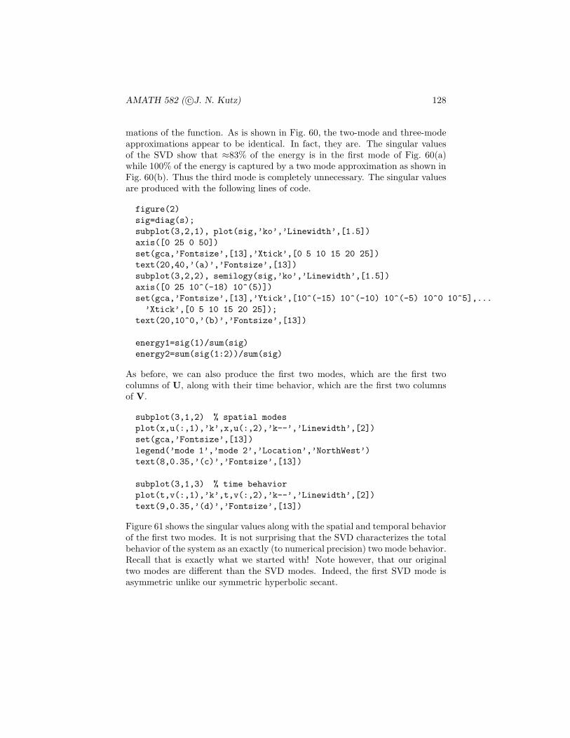
AMATH 582 ( c©J. N. Kutz) 128
mations of the function. As is shown in Fig. 60, the two-mode and three-modeapproximations appear to be identical. In fact, they are. The singular valuesof the SVD show that ≈83% of the energy is in the first mode of Fig. 60(a)while 100% of the energy is captured by a two mode approximation as shown inFig. 60(b). Thus the third mode is completely unnecessary. The singular valuesare produced with the following lines of code.
figure(2)
sig=diag(s);
subplot(3,2,1), plot(sig,’ko’,’Linewidth’,[1.5])
axis([0 25 0 50])
set(gca,’Fontsize’,[13],’Xtick’,[0 5 10 15 20 25])
text(20,40,’(a)’,’Fontsize’,[13])
subplot(3,2,2), semilogy(sig,’ko’,’Linewidth’,[1.5])
axis([0 25 10^(-18) 10^(5)])
set(gca,’Fontsize’,[13],’Ytick’,[10^(-15) 10^(-10) 10^(-5) 10^0 10^5],...
’Xtick’,[0 5 10 15 20 25]);
text(20,10^0,’(b)’,’Fontsize’,[13])
energy1=sig(1)/sum(sig)
energy2=sum(sig(1:2))/sum(sig)
As before, we can also produce the first two modes, which are the first twocolumns of U, along with their time behavior, which are the first two columnsof V.
subplot(3,1,2) % spatial modes
plot(x,u(:,1),’k’,x,u(:,2),’k--’,’Linewidth’,[2])
set(gca,’Fontsize’,[13])
legend(’mode 1’,’mode 2’,’Location’,’NorthWest’)
text(8,0.35,’(c)’,’Fontsize’,[13])
subplot(3,1,3) % time behavior
plot(t,v(:,1),’k’,t,v(:,2),’k--’,’Linewidth’,[2])
text(9,0.35,’(d)’,’Fontsize’,[13])
Figure 61 shows the singular values along with the spatial and temporal behaviorof the first two modes. It is not surprising that the SVD characterizes the totalbehavior of the system as an exactly (to numerical precision) two mode behavior.Recall that is exactly what we started with! Note however, that our originaltwo modes are different than the SVD modes. Indeed, the first SVD mode isasymmetric unlike our symmetric hyperbolic secant.

AMATH 582 ( c©J. N. Kutz) 129
0 5 10 15 20 250
20
40 (a)
0 5 10 15 20 25
10−15
10−10
10−5
100
105
(b)
−10 −8 −6 −4 −2 0 2 4 6 8 10−0.5
0
0.5
(c)mode 1mode 2
0 1 2 3 4 5 6 7 8 9 10−0.4
−0.2
0
0.2
0.4 (d)
Figure 61: Singular values on a standard plot (a) and a log plot (b) showing theenergy in each POD mode. For the space-time surface considered in Fig. 60,the bulk of the energy is in the first POD mode. A two mode approximationproduces 100% of the energy. The linear POD modes are illustrated in panel(c) which their time evolution behavior in panel (d).
Summary and Limits of SVD/PCA/POD
The methods of PCA and POD, which are essentially related to the idea ofdiagonalization of any matrix via the SVD, are exceptionally powerful tools andmethods for the evaluation data driven systems. Further, they provide the mostprecise method for performing low-dimensional reductions of a given system. Anumber of key steps are involved in applying the method to experimental orcomputational data sets.
• Organize the data into a matrix A ∈ Cm×n where m is the number ofmeasurement types (or probes) and n is the number of measurements (ortrials) taken from each probe.
• Subtract off the mean for each measurement type or row xj .
• Compute the SVD and singular values of the covariance matrix to deter-mine the principal components.
If considering a fitting algorithm, then the POD method is the appropriatetechnique to consider and the SVD can be applied directly to the A ∈ Cm×n
AMATH 582 ( c©J. N. Kutz) 130
matrix. This then produces the singular values as well as the POD modes ofinterest.
Although extremely powerful, and seemingly magical in its ability to pro-duce insightful quantification of a given problem, these SVD methods are notwithout limits. Some fundamental assumptions have been made in producingthe results thus far, the most important being the assumption of linearity. Re-cently some efforts to extend the method using nonlinearity prior to the SVDhave been explored [16, 17, 18]. A second assumption is that larger variances(singular values) represent more important dynamics. Although generally this isbelieved to be true, there are certainly cases where this assumption can be quitemisleading. Additionally, in constructing the covariance matrix, it is assumedthat the mean and variance are sufficient statistics for capturing the underlyingthe dynamics. It should be noted that only exponential (Gaussian) probabilitydistributions are completely characterized by the first two moments of the data.This will be considered further in the next section on independent componentanalysis. Finally, it is often the case that PCA may not produce the optimalresults. For instance, consider a point on a propeller blade. Viewed from thePCA framework, two orthogonal components are produced to describe the cir-cular motion. However, this is really a one-dimensional system that is solelydetermined by the phase variable. The PCA misses this fact unless use is madeof the information already known, i.e. that a polar coordinate system with fixedradius is the appropriate context to frame the problem. Thus blindly applyingthe technique can also lead to non-optimal results that miss obvious facts.
5 Independent Component Analysis
The concept of principal components or of a proper orthogonal decompositionare fundamental to data analysis. Essentially, there is an assertion, or perhapsa hope, that underlying seemingly complex and unordered data, there is in fact,some characteristic, and perhaps low-dimensional ordering of the data. Thesingular value decomposition of a matrix, although a mathematical idea, wasactually a formative tool for the interpretation and ordering of the data. In thissection on independent component analysis (ICA), the ideas turn to data setsfor which there are more than one statistically independent objects in the data.ICA provides a foundational mathematical method for extracting interleaveddata sets in a fairly straightforward way. Its applications are wide and varied,but our primary focus will be application of ICA in the context of image analysis.
5.1 The concept of independent components
Independent component analysis (ICA) is a powerful tool that extends the con-cepts of PCA, POD and SVD. Moreover, you are already intuitively familiarwith the concept as some of the examples here will show. A simple way to

AMATH 582 ( c©J. N. Kutz) 131
!"#$%&'()"#*+* !"#$%&'()"#*,*
-.!&"/0"#%*+*
-.!&"/0"#%*,*
Figure 62: Envisioned cocktail party problem. Two groups of people are havingseparate conversations which are recorded from microphone one and two. Thesignals from the two conversations are mixed together at microphone one andtwo according to the placement relative to the conversations. From the twomicrophone recordings, the individual conversations can then be extracted.
motivate thinking about ICA is by considering the cocktail party problem. Thusconsider two conversations in a room that are happening simultaneously. Howis it that the two different acoustic signals of conversation one and two can beseparated out? Figure 62 depicts a scenario where two groups are conversing.Two microphones are placed in the room at different spatial locations and fromthe two signals s1(t) and s2(t) a mathematical attempt is made to separate thesignals that have been mixed at each of the microphone locations. Provided thatthe noise level is not too large or that the conversation volumes are sufficientlylarge, humans can perform this task with remarkable ease. In our case, thetwo microphones are our two ears. Indeed, this scenario and its mathematicalfoundations are foundational to the concept of eavesdropping on a conversation.
From a mathematical standpoint, this problem can be formulated with thefollowing mixing equation
x1(t) = a11s1 + a12s2 (5.1.126a)
x2(t) = a21s1 + a22s2 (5.1.126b)
where x1(t) and x2(t) are the mixed, recorded signals at microphone one and tworespectively. The coefficients aij are the mixing parameters that are determinedby a variety of factors including the placement of the microphones in the room,the distance to the conversations, and the overall room acoustics. Note thatwe are omitting time-delay signals that may reflect off the walls of the room.This problem also resembles quite closely what may happen in a large numberof applications. For instance, consider the following
• Radar detection: If there are numerous targets that are being tracked,then there is significant mixing in the scattered signal from all of the
AMATH 582 ( c©J. N. Kutz) 132
targets. Without a method for clear separation of the targets, the detectorbecomes useless for identifying location.
• Electroencephalogram (EEG): EEG readings are electrical recordingsof brain activities. Typically these EEG readings are from multiple loca-tions of the scalp. However, at each EEG reading location, all the brainactivity signals are mixed, thus preventing a clear understanding of howmany underlying signals are contained within. With a large number ofEEG probes, ICA allows for the separation of the brain activity readingsand a better assessment of the overall neural activity.
• Terminator Salvation: If you remember in the movie, John Connorand the resistance found a hidden signal (ICA) embedded on the normalsignals in the communications sent between the terminators and skynetvehicles and ships. Although not mentioned in the movie, this was clearlysomebody in the future who is taking AMATH 582 now. Somehow thatbit of sweet math only made it to the cutting room floor. Regardless, oneshouldn’t under-restimate how awesome data analysis skills are in the realworld of the future.
The ICA method is closely related to the blind source separation (BSS) (orblind signal separation) method. Here the sources refer to the original signals,or independent components, and blind refers to the fact that the mixing matrixcoefficients aij are unknown.
A more formal mathematical framework for ICA can be established by con-sidering the following: Given N distinct linear combinations of N signals (ordata sets), determine the original N images. This is the succinct statementof the mathematical objective of ICA. Thus to generalize (5.1.126) to the Ndimensional system we have
xj(t) = aj1s1 + aj2s2 + · · · + ajNsN 1 ≤ j ≤ N . (5.1.127)
Expressed in matrix form, this results in
x = As (5.1.128)
where x are the mixed signal measurements, s are the original signals we aretrying to determine, and A is the matrix of coefficients which determines howthe signals are mixed as a function of the physical system of interest. At first,one might simply say that the solution to this is trivial and it is given by
s = A−1x (5.1.129)
where we are assuming that the placement of our measurement devices are suchthat A is nonsingular and its inverse exists. Such a solution makes the followingassumption: we know the matrix cofficients aij . The point is, we don’t know
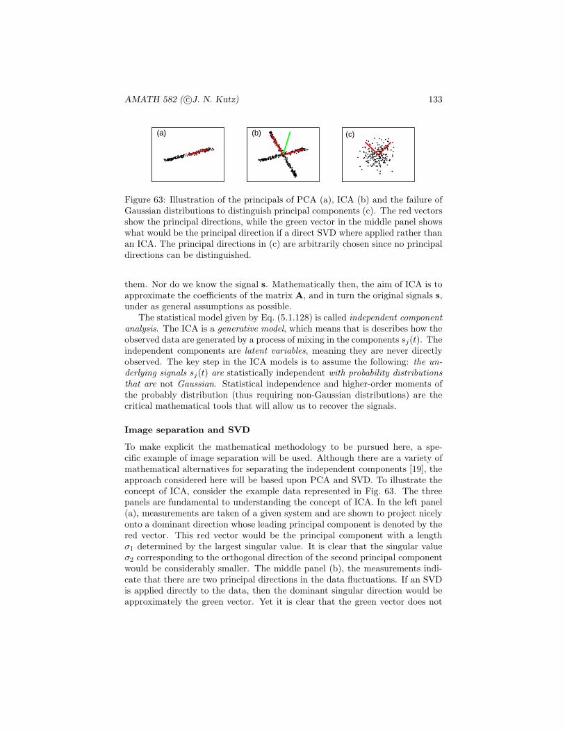
AMATH 582 ( c©J. N. Kutz) 133
(a) (b) (c)
Figure 63: Illustration of the principals of PCA (a), ICA (b) and the failure ofGaussian distributions to distinguish principal components (c). The red vectorsshow the principal directions, while the green vector in the middle panel showswhat would be the principal direction if a direct SVD where applied rather thanan ICA. The principal directions in (c) are arbitrarily chosen since no principaldirections can be distinguished.
them. Nor do we know the signal s. Mathematically then, the aim of ICA is toapproximate the coefficients of the matrix A, and in turn the original signals s,under as general assumptions as possible.
The statistical model given by Eq. (5.1.128) is called independent componentanalysis. The ICA is a generative model, which means that is describes how theobserved data are generated by a process of mixing in the components sj(t). Theindependent components are latent variables, meaning they are never directlyobserved. The key step in the ICA models is to assume the following: the un-derlying signals sj(t) are statistically independent with probability distributionsthat are not Gaussian. Statistical independence and higher-order moments ofthe probably distribution (thus requiring non-Gaussian distributions) are thecritical mathematical tools that will allow us to recover the signals.
Image separation and SVD
To make explicit the mathematical methodology to be pursued here, a spe-cific example of image separation will be used. Although there are a variety ofmathematical alternatives for separating the independent components [19], theapproach considered here will be based upon PCA and SVD. To illustrate theconcept of ICA, consider the example data represented in Fig. 63. The threepanels are fundamental to understanding the concept of ICA. In the left panel(a), measurements are taken of a given system and are shown to project nicelyonto a dominant direction whose leading principal component is denoted by thered vector. This red vector would be the principal component with a lengthσ1 determined by the largest singular value. It is clear that the singular valueσ2 corresponding to the orthogonal direction of the second principal componentwould be considerably smaller. The middle panel (b), the measurements indi-cate that there are two principal directions in the data fluctuations. If an SVDis applied directly to the data, then the dominant singular direction would beapproximately the green vector. Yet it is clear that the green vector does not

AMATH 582 ( c©J. N. Kutz) 134
!"#$%"&
'()*+&,-.%!$&
Figure 64: Illustration of image separation problem. A piece of glass reflectspart of the background light source while some of the light penetrates to theimage and is reflected to the camera. Thus the camera sees two images: theimage (painting) and the reflection of the background light source.
accurately represent the data. Rather, the data seems to be organized inde-pedently along two different directions. An SVD of the two independent datasets would produce two principal components, i.e. two independent componentanalysis vectors. Thus it is critical to establish a method for separating outdata of this sort into their independent directions. Finally, in the third panel(c), Gaussian distributed data is shown where no principal components can beidentified with certainty. Indeed, there are an infinite number of possible orthog-onal projections that can be made. Two arbitrary directions have been shownin panel (c). This graphic shows why Gaussian distributed random variablesare disastrous for ICA, no projections onto the independent components can beaccomplished.
We now turn our attention to the issue of image separation. Figure 64demonstrates a prototypical example of what can occur when photographingan image behind glass. The glass encasing of the art work, or image, producesa reflection of the backlit source along with the image itself. Amazingly, thehuman eye can very easily compensate for this and see through much of thereflection to the original image. Alternatively, if we choose, we can also focuson the reflected image of the backlit source. Ultimately, there is some interestin training a computer to do this image processing automatically. Indeed, inartificial vision, algorithms such as these are important for mimicking naturalhuman behaviors and abilities.
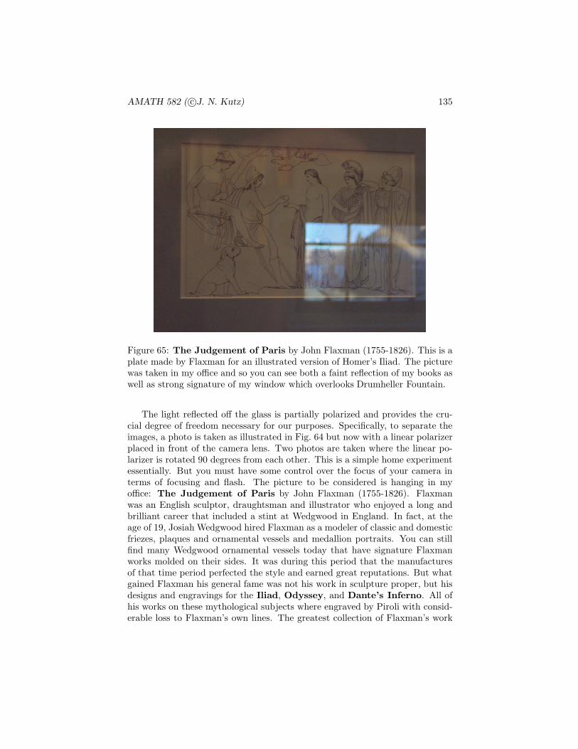
AMATH 582 ( c©J. N. Kutz) 135
Figure 65: The Judgement of Paris by John Flaxman (1755-1826). This is aplate made by Flaxman for an illustrated version of Homer’s Iliad. The picturewas taken in my office and so you can see both a faint reflection of my books aswell as strong signature of my window which overlooks Drumheller Fountain.
The light reflected off the glass is partially polarized and provides the cru-cial degree of freedom necessary for our purposes. Specifically, to separate theimages, a photo is taken as illustrated in Fig. 64 but now with a linear polarizerplaced in front of the camera lens. Two photos are taken where the linear po-larizer is rotated 90 degrees from each other. This is a simple home experimentessentially. But you must have some control over the focus of your camera interms of focusing and flash. The picture to be considered is hanging in myoffice: The Judgement of Paris by John Flaxman (1755-1826). Flaxmanwas an English sculptor, draughtsman and illustrator who enjoyed a long andbrilliant career that included a stint at Wedgwood in England. In fact, at theage of 19, Josiah Wedgwood hired Flaxman as a modeler of classic and domesticfriezes, plaques and ornamental vessels and medallion portraits. You can stillfind many Wedgwood ornamental vessels today that have signature Flaxmanworks molded on their sides. It was during this period that the manufacturesof that time period perfected the style and earned great reputations. But whatgained Flaxman his general fame was not his work in sculpture proper, but hisdesigns and engravings for the Iliad, Odyssey, and Dante’s Inferno. All ofhis works on these mythological subjects where engraved by Piroli with consid-erable loss to Flaxman’s own lines. The greatest collection of Flaxman’s work

AMATH 582 ( c©J. N. Kutz) 136
is housed in the Flaxman Gallery at the University College London.In the specific Flaxman example considered here, one of the most famous
scenes of mythology is depicted: The Judgement of Paris. In this scene,Hermes watches as young Paris plays the part of judge. His task is to con-template giving the golden apple with the inscription To the Fairest to eitherVenus, Athena, or Hera. This golden apple was placed at the wedding receptionof Peleus and Thetis, father and mother of peerless Achilles, by Discord sinceshe did not receive a wedding invitation. Each lovely goddess in turn promiseshim something for the apple: Athena promises that he will become the greatestwarrior in history, Juno promises him to be greatest ruler in the land, ruling overa vast and unmatched empire. Last comes the lovely Venus who promises himthat the most beautiful woman in the world will be his. Of course, to sweeten upher offer, she is wearing next to nothing as usual. Lo and behold, the hot chickwins! And as a result we have the Trojan War for which Helen was fought for. Icould go on here, but what else is to be expected of a young 20-something yearold male (an older guy would have taken the vast kingdom while a prepubescentboy would have chosen to be the great warrior). It is comforting to know thatvery little has changed since in some 4000 years. Figures 65 and 66 representthis Flaxman scene along with the reflected image of my office window. Thetwo pictures are taken with a linear polarizer in front of a camera that has beenrotated by 90 degrees between the photos.
SVD method for ICA
Given the physical problem, how is SVD used then to separate the two imagesobserved in Figs. 65 and 66? Consider the action of the SVD on the image mixingmatrix A of Eq. (5.1.128). In this case, there are two images S1 and S2 thatwe are working with. This gives us 6 unknowns (S1,S2, a11, a12, a21, a22) withonly the two constraints from Eq. (5.1.128). Thus the system cannot be solvedwithout further assumptions being made. The first assumption will be that thetwo images are statistically independent. If the pixel intensities are denoted byS1 and S2, then statistical independence is mathematically expressed as
P (S1,S2) = P (S1)P (S2) (5.1.130)
which states that the joint probability density is separable. No specific form isplaced upon the probability densities themselves aside from this: they cannot beGaussian distributed. In practice, this is a reasonable constraint since naturalimages are rarely Gaussian. A second assumption is that the matrix A is fullrank, thus assuming that the two measurements of the image indeed have beenfiltered with different polarization states. These assumptions yield an estimationproblem which is the ICA.
Consider what happens under the SVD process to the matrix A
A = UΣV∗ (5.1.131)

AMATH 582 ( c©J. N. Kutz) 137
Figure 66: This is an identical picture to Fig. 65 with a linear polarizer rotated90 degrees. The polarization state of the reflected field is effected by the linearpolarizer, thus allowing us to separate the images.
where again U and V are unitary matrices that simply lead to rotation and Σstretches (scales) an image as prescribed by the singular values. A graphicalillustration of this process is shown in Fig. 67 for distributions that are uniform,i.e. they form a square. The mixing matrix A can be thought to first rotatethe square via unitary matrix V∗, then stretch it into a parallelogram via thediagonal matrix Σ and then rotate the parallelogram via the unitary matrix U.This is now the mixed image X. The estimation, or ICA, of the independentimages thus reduces to finding how to transform the rotated parallelogram backinto a square. Or mathematically, transforming the mixed image back into aseparable product of one-dimensional probability distributions. This is the defin-ing mathematical goal of the ICA image analysis problem, or any general ICAreduction technique.
5.2 Image separation problem
The method proposed here to separate two images relies on reversing the actionof the SVD on the two statistically independent images. Again, the matrixA in (5.1.131) is not known, so a direct computation of the SVD cannot beperformed. However, each of the individual matrices can be approximated byconsidering its net effect on the assumed uniformly distributed images.
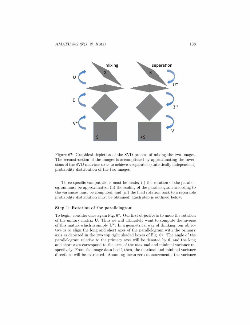
AMATH 582 ( c©J. N. Kutz) 138
!"
#"
$%"
!%"
#&'"
$"
()*)+," -./01023+"
4"
5" 5"
64"
Figure 67: Graphical depiction of the SVD process of mixing the two images.The reconstruction of the images is accomplished by approximating the inver-sions of the SVD matrices so as to achieve a separable (statistically independent)probability distribution of the two images.
Three specific computations must be made: (i) the rotation of the parallel-ogram must be approximated, (ii) the scaling of the parallelogram according tothe variances must be computed, and (iii) the final rotation back to a separableprobability distribution must be obtained. Each step is outlined below.
Step 1: Rotation of the parallelogram
To begin, consider once again Fig. 67. Our first objective is to undo the rotationof the unitary matrix U. Thus we will ultimately want to compute the inverseof this matrix which is simply U∗. In a geometrical way of thinking, our objec-tive is to align the long and short axes of the parallelogram with the primaryaxis as depicted in the two top right shaded boxes of Fig. 67. The angle of theparallelogram relative to the primary axes will be denoted by θ, and the longand short axes correspond to the axes of the maximal and minimal variance re-spectively. From the image data itself, then, the maximal and minimal variancedirections will be extracted. Assuming mean-zero measurements, the variance

AMATH 582 ( c©J. N. Kutz) 139
at an arbitrary angle of orientation is given by
V ar(θ) =
N∑
j=1
{[x1(j) x2(j)]
[cos θsin θ
]}2
. (5.2.132)
The maximal variance is determined by computing the angle θ that maximizesthis function. It will be assumed that the corresponding angle of minimal vari-ance will be orthogonal to this at θ−π/2. These axes are essentially the principalcomponent directions that would be computed if we actually knew componentsof the matrix A.
The maximum of (5.2.132) with respect to θ can be found by differentiatingV ar(θ) and setting it equal to zero. To do this, Eq. (5.2.132) is rewritten as
V ar(θ) =
N∑
j=1
{[x1(j) x2(j)]
[cos θsin θ
]}2
=N∑
j=1
[x1(j) cos θ + x2(j) sin θ]2 (5.2.133)
=
N∑
j=1
x21(j) cos2 θ + 2x1(j)x2(j) cos θ sin θ + x2
2(j) sin2 θ.
Differentiating with respect to θ then gives
d
dθV ar(θ) = 2
N∑
j=1
−x21(j) sin θ cos θ+x1(j)x2(j)
[cos2 θ−sin2 θ
]+x2
2(j) sin θ cos θ
= 2
N∑
j=1
[x2
2(j) − x21(j)
]sin θ cos θ + x1(j)x2(j)
[cos2 θ − sin2 θ
]
=N∑
j=1
[x2
2(j) − x21(j)
]sin 2θ + 2x1(j)x2(j) cos 2θ (5.2.134)
which upon setting this equal to zero gives the value of θ desired. Thus takingd(V ar(θ))/dθ = 0 gives
sin 2θ
cos 2θ=
−2∑Nj=1 x1(j)x2(j)
∑Nj=1 x
22(j) − x2
1(j), (5.2.135)
or in terms of θ alone
θ0 =1
2tan−1
[−2
∑Nj=1 x1(j)x2(j)
∑Nj=1 x
22(j) − x2
1(j)
]. (5.2.136)
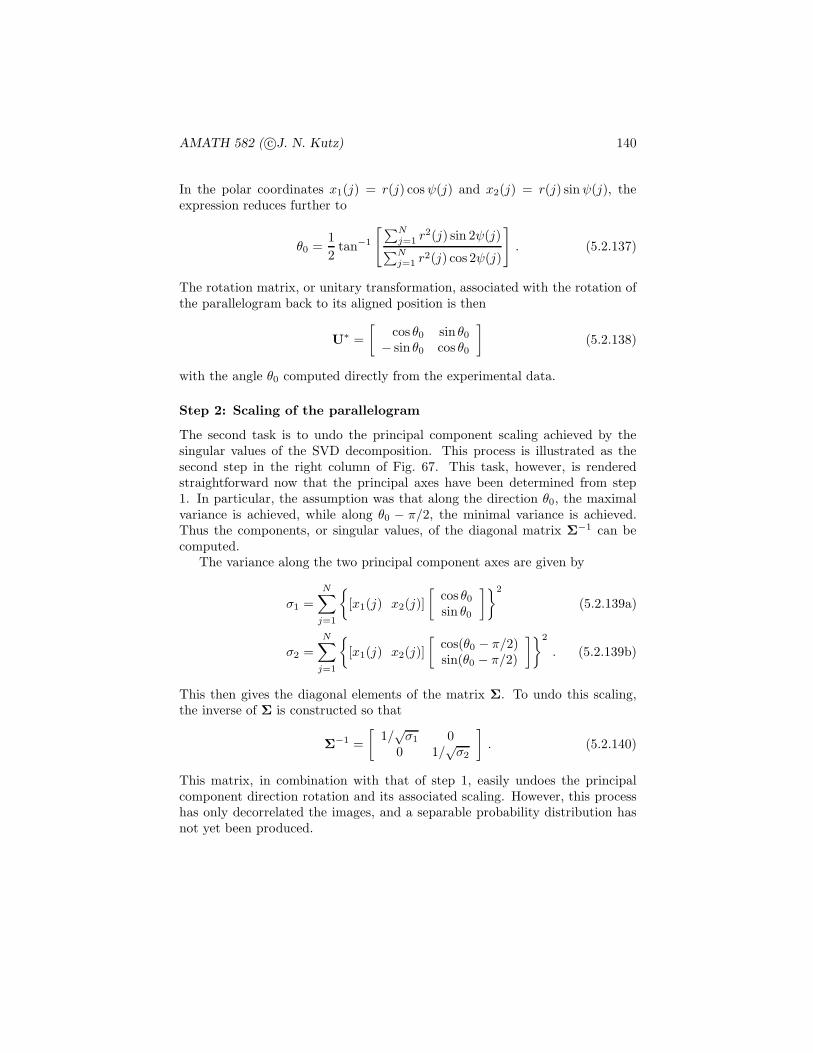
AMATH 582 ( c©J. N. Kutz) 140
In the polar coordinates x1(j) = r(j) cosψ(j) and x2(j) = r(j) sinψ(j), theexpression reduces further to
θ0 =1
2tan−1
[ ∑Nj=1 r
2(j) sin 2ψ(j)∑N
j=1 r2(j) cos 2ψ(j)
]. (5.2.137)
The rotation matrix, or unitary transformation, associated with the rotation ofthe parallelogram back to its aligned position is then
U∗ =
[cos θ0 sin θ0
− sin θ0 cos θ0
](5.2.138)
with the angle θ0 computed directly from the experimental data.
Step 2: Scaling of the parallelogram
The second task is to undo the principal component scaling achieved by thesingular values of the SVD decomposition. This process is illustrated as thesecond step in the right column of Fig. 67. This task, however, is renderedstraightforward now that the principal axes have been determined from step1. In particular, the assumption was that along the direction θ0, the maximalvariance is achieved, while along θ0 − π/2, the minimal variance is achieved.Thus the components, or singular values, of the diagonal matrix Σ−1 can becomputed.
The variance along the two principal component axes are given by
σ1 =
N∑
j=1
{[x1(j) x2(j)]
[cos θ0sin θ0
]}2
(5.2.139a)
σ2 =
N∑
j=1
{[x1(j) x2(j)]
[cos(θ0 − π/2)sin(θ0 − π/2)
]}2
. (5.2.139b)
This then gives the diagonal elements of the matrix Σ. To undo this scaling,the inverse of Σ is constructed so that
Σ−1 =
[1/
√σ1 0
0 1/√σ2
]. (5.2.140)
This matrix, in combination with that of step 1, easily undoes the principalcomponent direction rotation and its associated scaling. However, this processhas only decorrelated the images, and a separable probability distribution hasnot yet been produced.

AMATH 582 ( c©J. N. Kutz) 141
Step 3: Rotation to produce a separable probability distribution
The final rotation to separate the probability distributions is a more subtle andrefined issue, but critical to producing nearly separable probability distributions.This separation process typically relies on the higher moments of the probabilitydistribution. Since the mean has been assumed to be zero and there is noreason to believe that there is an asymmetry in the probability distributions,i.e. higher-order odd moments (such as the skewness) are negligible, the nextdominant statistical moment to consider is the fourth moment, or the kurtosisof the probability distribution. The goal will be to minimize this fourth-ordermoment, and by doing so we will determine the appropriate rotation angle.Note that the second moment has already been handled through steps and 1and 2. Said in a different mathematical way, minimizing the kurtosis will beanother step in trying to approximate the probability distribution of the imagesas separable functions so that P (S1S2) ≈ P (S1)P (S2).
The kurtosis of a probability distribution is given by
kurt(φ) = K(φ) =
N∑
j=1
{[x1(j) x2(j)]
[cosφsinφ
]}4
(5.2.141)
where φ is the angle of rotation associated with the unitary matrix U and thevariables x1(j) and x2(j) is the image that has undergone the two steps oftransformation as outlined previously.
For analytic convenience, a normalized version of the above definition ofkurtosis will be considered. Specifically, a normalized version is computed inpractice. The expedience of the normalization will become clear through thealgebraic manipulations. Thus consider
K(φ) =
N∑
j=1
1
x21(j) + x2
2(j)
{[x1(j) x2(j)]
[cosφsinφ
]}4
. (5.2.142)
As in our calculation regarding the second moment, the kurtosis will be writtenin a more natural form for differentiation
K(φ) =
N∑
j=1
1
x21(j) + x2
2(j)
{[x1(j) x2(j)]
[cosφsinφ
]}4
=N∑
j=1
1
x21(j) + x2
2(j)[x1(j) cosφ+ x2(j) sinφ]4 (5.2.143)
=
N∑
j=1
1
x21(j) + x2
2(j)
[x4
1(j) cos4 φ+ 4x31(j)x2(j) cos3 φ sinφ
+6x21(j)x
22(j) cos2 φ sin2 φ+ 4x1(j)x
32(j) cosφ sin3 φ+ x4
2(j) sin4 φ]
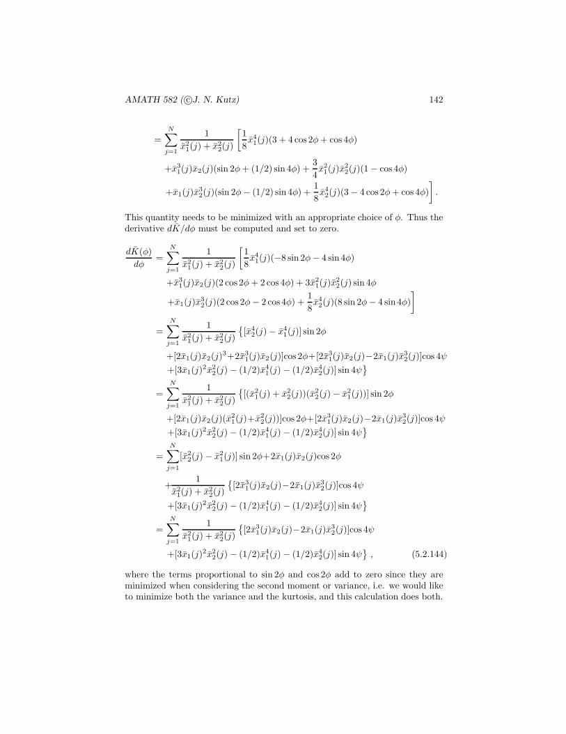
AMATH 582 ( c©J. N. Kutz) 142
=
N∑
j=1
1
x21(j) + x2
2(j)
[1
8x4
1(j)(3 + 4 cos 2φ+ cos 4φ)
+x31(j)x2(j)(sin 2φ+ (1/2) sin 4φ) +
3
4x2
1(j)x22(j)(1 − cos 4φ)
+x1(j)x32(j)(sin 2φ− (1/2) sin 4φ) +
1
8x4
2(j)(3 − 4 cos 2φ+ cos 4φ)
].
This quantity needs to be minimized with an appropriate choice of φ. Thus thederivative dK/dφ must be computed and set to zero.
dK(φ)
dφ=
N∑
j=1
1
x21(j) + x2
2(j)
[1
8x4
1(j)(−8 sin 2φ− 4 sin 4φ)
+x31(j)x2(j)(2 cos 2φ+ 2 cos 4φ) + 3x2
1(j)x22(j) sin 4φ
+x1(j)x32(j)(2 cos 2φ− 2 cos 4φ) +
1
8x4
2(j)(8 sin 2φ− 4 sin 4φ)
]
=
N∑
j=1
1
x21(j) + x2
2(j)
{[x4
2(j) − x41(j)] sin 2φ
+[2x1(j)x2(j)3+2x3
1(j)x2(j)]cos 2φ+[2x31(j)x2(j)−2x1(j)x
32(j)]cos 4ψ
+[3x1(j)2x2
2(j) − (1/2)x41(j) − (1/2)x4
2(j)] sin 4ψ}
=
N∑
j=1
1
x21(j) + x2
2(j)
{[(x2
1(j) + x22(j))(x
22(j) − x2
1(j))] sin 2φ
+[2x1(j)x2(j)(x21(j)+x
22(j))]cos 2φ+[2x3
1(j)x2(j)−2x1(j)x32(j)]cos 4ψ
+[3x1(j)2x2
2(j) − (1/2)x41(j) − (1/2)x4
2(j)] sin 4ψ}
=N∑
j=1
[x22(j) − x2
1(j)] sin 2φ+2x1(j)x2(j)cos 2φ
+1
x21(j) + x2
2(j)
{[2x3
1(j)x2(j)−2x1(j)x32(j)]cos 4ψ
+[3x1(j)2x2
2(j) − (1/2)x41(j) − (1/2)x4
2(j)] sin 4ψ}
=
N∑
j=1
1
x21(j) + x2
2(j)
{[2x3
1(j)x2(j)−2x1(j)x32(j)]cos 4ψ
+[3x1(j)2x2
2(j) − (1/2)x41(j) − (1/2)x4
2(j)] sin 4ψ}, (5.2.144)
where the terms proportional to sin 2φ and cos 2φ add to zero since they areminimized when considering the second moment or variance, i.e. we would liketo minimize both the variance and the kurtosis, and this calculation does both.

AMATH 582 ( c©J. N. Kutz) 143
By setting this to zero, the angle φ0 can be determined to be
φ0 =1
4tan−1
[−∑N
j=1[2x31(j)x2(j)−2x1(j)x
32(j)]/[x
21(j) + x2
2(j)]∑Nj=1[3x1(j)2x2
2(j) − (1/2)x41(j) − (1/2)x4
2(j)]/[x21(j) + x2
2(j)]
]
(5.2.145)When converted to polar coordinates, this reduces very nicely to the followingexpression:
φ0 =1
4tan−1
[ ∑Nj=1 r
2 sin 4ψ(j)∑Nj=1 r
2 cos 4ψ(j)
](5.2.146)
The rotation back to the approximately statistically independent square is thengiven by
V =
[cosφ0 sinφ0
− sinφ0 cosφ0
](5.2.147)
with the angle θ0 computed directly from the experimental data. At this point,it is unknown wether the angle φ0 is a minimum or maximum of the kurtosisand this should be checked. Sometimes this is a maximum, especially in caseswhen one of the image histograms has long tails relative to the other [20].
Completing the analysis
Recall that our purpose was to compute, through the statistics of the images(pixels) themselves, the SVD decomposition. The method relied on computing(approximating) the principal axis and scaling of the principal components.The final piece was to try and make the probability distribution as separable aspossible by minimizing the kurtosis as a function of the final rotation angle.
To reconstruct the image, the following linear algebra operation is performed:
s=A−1x = VΣ−1U∗x
=
[cosφ0 sinφ0
− sinφ0 cosφ0
][1/
√σ1 0
0 1/√σ2
][cos θ0 sin θ0
− sin θ0 cos θ0
]x (5.2.148)
A few things should be noted about the inherent ambiguities in the recovery ofthe two images. The first is the ordering ambiguity. Namely, the two matricesare indistinguishable:
[a11 a12
a21 a22
] [x1
x2
]=
[a21 a22
a11 a12
] [x2
x1
](5.2.149)
Thus image one and two are arbitrary to some extent. In practice this does notmatter since the aim was simply to separate, not label, the data measurements.There is also an ambiguity in the scaling since
[a11 a12
a21 a22
] [x1
x2
]=
[a11/α a12/δa21/α a22/δ
] [αx1
δx2
]. (5.2.150)

AMATH 582 ( c©J. N. Kutz) 144
Figure 68: Two images of Sicily: an ocean view from the hills of Erice and aninterior view of the Capella Palatina in Palermo.
Again this does not matter since the two separated images can then be rescaledto their full intensity range afterwards. Regardless, this shows the basic processthat needs to be applied to the system data in order to construct a self-consistentalgorithm capable of image separation.
5.3 Image separation and MATLAB
Using MATLAB, the previously discussed algorithm will be implemented. How-ever, before proceeding to try and extract the images displayed in Figs. 65 and66, a more idealized case is considered. Consider the two ideal images of Sicilyin Fig. 68. These two images will be mixed with two different weights to pro-duce two mixed images. Our objective will be to use the algorithm outlined inthe last section to separate out the images. Upon separation, the images can becompared with the ideal representation of Fig. 68. To load in the images andstart the processing, the following MATLAB commands are used.
S1=imread(’sicily1’,’jpeg’);
S2=imread(’sicily2’,’jpeg’);
subplot(2,2,1), imshow(S1);
subplot(2,2,2), imshow(S2);
The two images are quite different with one overlooking the mediterranean fromthe medieval village of Erice on the Northwest corner, and the second is ofthe Capella Palatina in Palermo. Recall that what is required is statisticalindependence of the two images. Thus the pixel strengths and colors should belargely decorrolated throughout the image.
The two ideal images are now mixed with the matrix A in Eq. (5.1.128).Specifically, we will consider the arbitrarily chosen mixing of the form
A =
[a11 a12
a21 a22
]=
[4/5 β1/2 2/3
](5.3.151)
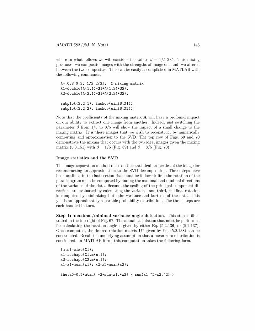
AMATH 582 ( c©J. N. Kutz) 145
where in what follows we will consider the values β = 1/5, 3/5. This mixingproduces two composite images with the strengths of image one and two alteredbetween the two composites. This can be easily accomplished in MATLAB withthe following commands.
A=[0.8 0.2; 1/2 2/3]; % mixing matrix
X1=double(A(1,1)*S1+A(1,2)*S2);
X2=double(A(2,1)*S1+A(2,2)*S2);
subplot(2,2,1), imshow(uint8(X1));
subplot(2,2,2), imshow(uint8(X2));
Note that the coefficients of the mixing matrix A will have a profound impacton our ability to extract one image from another. Indeed, just switching theparameter β from 1/5 to 3/5 will show the impact of a small change to themixing matrix. It is these images that we wish to reconstruct by numericallycomputing and approximation to the SVD. The top row of Figs. 69 and 70demonstrate the mixing that occurs with the two ideal images given the mixingmatrix (5.3.151) with β = 1/5 (Fig. 69) and β = 3/5 (Fig. 70).
Image statistics and the SVD
The image separation method relies on the statistical properties of the image forreconstructing an approximation to the SVD decomposition. Three steps havebeen outlined in the last section that must be followed: first the rotation of theparallelogram must be computed by finding the maximal and minimal directionsof the variance of the data. Second, the scaling of the principal component di-rections are evaluated by calculating the variance, and third, the final rotationis computed by minimizing both the variance and kurtosis of the data. Thisyields an approximately separable probability distribution. The three steps areeach handled in turn.
Step 1: maximal/minimal variance angle detection. This step is illus-trated in the top right of Fig. 67. The actual calculation that must be performedfor calculating the rotation angle is given by either Eq. (5.2.136) or (5.2.137).Once computed, the desired rotation matrix U∗ given by Eq. (5.2.138) can beconstructed. Recall the underlying assumption that a mean-zero distribution isconsidered. In MATLAB form, this computation takes the following form.
[m,n]=size(X1);
x1=reshape(X1,m*n,1);
x2=reshape(X2,m*n,1);
x1=x1-mean(x1); x2=x2-mean(x2);
theta0=0.5*atan( -2*sum(x1.*x2) / sum(x1.^2-x2.^2) )
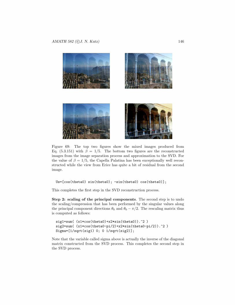
AMATH 582 ( c©J. N. Kutz) 146
Figure 69: The top two figures show the mixed images produced fromEq. (5.3.151) with β = 1/5. The bottom two figures are the reconstructedimages from the image separation process and approximation to the SVD. Forthe value of β = 1/5, the Capella Palatina has been exceptionally well recon-structed while the view from Erice has quite a bit of residual from the secondimage.
Us=[cos(theta0) sin(theta0); -sin(theta0) cos(theta0)];
This completes the first step in the SVD reconstruction process.
Step 2: scaling of the principal components. The second step is to undothe scaling/compression that has been performed by the singular values alongthe principal component directions θ0 and θ0 − π/2. The rescaling matrix thusis computed as follows:
sig1=sum( (x1*cos(theta0)+x2*sin(theta0)).^2 )
sig2=sum( (x1*cos(theta0-pi/2)+x2*sin(theta0-pi/2)).^2 )
Sigma=[1/sqrt(sig1) 0; 0 1/sqrt(sig2)];
Note that the variable called sigma above is actually the inverse of the diagonalmatrix constructed from the SVD process. This completes the second step inthe SVD process.

AMATH 582 ( c©J. N. Kutz) 147
Figure 70: The top two figures show the mixed images produced fromEq. (5.3.151) with β = 3/5. The bottom two figures are the reconstructedimages from the image separation process and approximation to the SVD. Forthe value of β = 3/5, the view from Erice has been has been well reconstructedaside from the top right corner of the image while the Capella Palatina remainsof poor quality.
Step 3: rotation to separability. The final rotation is aimed towards pro-ducing, as best as possible, a separable probability distribution. The analyticmethod used to do this is to minimize both the variance and kurtosis of theremaining distributions. The angle that accomplishes this task is computedanalytically from either (5.2.145) or (5.2.146) and the associated rotation ma-trix V is given by (5.2.147). Before computing this final rotation, the imageafter steps 1 and 2 must be produced, i.e. we compute the X1 and X2 used in(5.2.145) and (5.2.146). The MATLAB code used to produce the final rotationmatrix is then
X1bar= Sigma(1,1)*(Us(1,1)*X1+Us(1,2)*X2);
X2bar= Sigma(2,2)*(Us(2,1)*X1+Us(2,2)*X2);
x1bar=reshape(X1bar,m*n,1);
x2bar=reshape(X2bar,m*n,1);
phi0=0.25*atan( -sum(2*(x1bar.^3).*x2bar-2*x1bar.*(x2bar.^3)) ...

AMATH 582 ( c©J. N. Kutz) 148
Figure 71: The Judgement of Paris by Flaxman with a reflection of mywindow which overlooks Drumheller Fountain. In the top row are the twooriginal photos taken with linear polarizer rotated 90 degrees between shots.The bottom row represents the separated images. The brightness of the reflectedimage greatly effects the quality of the image separation.
/ sum(3*(x1bar.^2).*(x2bar.^2)-0.5*(x1bar.^4)-0.5*(x2bar.^4)) )
V=[cos(phi0) sin(phi0); -sin(phi0) cos(phi0)];
S1bar=V(1,1)*X1bar+V(1,2)*X2bar;
S2bar=V(2,1)*X1bar+V(2,2)*X2bar;
This final rotation completes the three steps of computing the SVD matrix.However, the images needed to be rescaled back to the full image brilliance.Thus the data points need to be made positive and scaled back to values rangingfrom 1 (dim) to 255 (bright). This final bit of code rescales and plots theseparated images.
min1=min(min(min(S1bar)));
S1bar=S1bar+min1;
max1=max(max(max(S1bar)));
S1bar=S1bar*(255/max1);
min2=min(min(min(S2bar)));

AMATH 582 ( c©J. N. Kutz) 149
S2bar=S2bar+min2;
max2=max(max(max(S2bar)));
S2bar=S2bar*(255/max2);
subplot(2,2,3), imshow(uint8(S1bar))
subplot(2,2,4), imshow(uint8(S2bar))
Note that the successive use of the min/max command is due to the fact thatthe color images are m×n×3 matrices where the 3 levels give the color mappinginformation.
Image separation from reflection
The algorithm above can be applied to the original problem presented of theJudgement of Paris by Flaxman. The original images are again illustrated inthe top row of Fig. 71. The difference in the two figures was the application ofa polarizer whose angle was rotated 90 degrees between shots. The bottom twofigures shows the extraction process that occurs for the two images. Ultimately,the technique applied here did not do such a great job. This is largely due tothe fact that the reflected image was so significantly brighter than the originalphotographed image itself, thus creating a difficult image separation problem.Certainly experience tells us that we also have this same difficulty: when it isvery bright and sunny out, reflected images are much more difficult for us tosee through to the true image.
6 Image Recognition
One of the most intriguing mathematical developments of the past decade con-cerns the ideas of image recognition. In particular, mathematically plausiblemethods are being rapidly developed to mimic real biological processes towardsautomating computers to recognize people, animals, and places. Indeed, thereare many applications, many of them available on smart phones, that can per-form sophisticated algorithms for doing the following: tag all images in a photolibrary with a specific person, and automatically identify the location and namea set of mountain peaks given a photo of the mountains. These image recog-nition methods are firmly rooted in the basic mathematical techniques to bedescribed in the following sections. It is remarkable the pace of this technologyand its potential for scientific impact. The methods here will bring togetherstatistics, time-frequency analysis and the SVD.
6.1 Recognizing dogs and cats
A basic and plausible methodology will be formulated in the context of imagerecognition. Specifically, we will generate a mathematically plausible mechanism
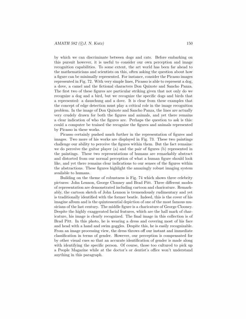
AMATH 582 ( c©J. N. Kutz) 150
by which we can discriminate between dogs and cats. Before embarking onthis pursuit however, it is useful to consider our own perception and imagerecognition capabilities. To some extent, the art world has been far ahead tothe mathematicians and scientists on this, often asking the question about howa figure can be minimally represented. For instance, consider the Picasso imagesrepresented in Fig. 72. With very simple lines, Picasso is able to represent a dog,a dove, a camel and the fictional characters Don Quixote and Sancho Panza.The first two of these figures are particular striking given that not only do werecognize a dog and a bird, but we recognize the specific dogs and birds thata represented: a dauschung and a dove. It is clear from these examples thatthe concept of edge detection must play a critical role in the image recognitionproblem. In the image of Don Quixote and Sancho Panza, the lines are actuallyvery crudely drawn for both the figures and animals, and yet there remainsa clear indication of who the figures are. Perhaps the question to ask is this:could a computer be trained the recognize the figures and animals representedby Picasso in these works.
Picasso certainly pushed much further in the representation of figures andimages. Two more of his works are displayed in Fig. 73. These two paintingschallenge our ability to perceive the figures within them. But the fact remains:we do perceive the guitar player (a) and the pair of figures (b) represented inthe paintings. These two representations of humans are remarkably abstractand distorted from our normal perception of what a human figure should looklike, and yet there remains clear indications to our senses of the figures withinthe abstractions. These figures highlight the amazingly robust imaging systemavailable to humans.
Building on the theme of robustness is Fig. 74 which shows three celebritypictures: John Lennon, George Clonney and Brad Pitt. Three different modesof representation are demonstrated including cartoon and charicature. Remark-ably, the cartoon sketch of John Lennon is tremendously rudimentary and yetis traditionally identified with the former beatle. Indeed, this is the cover of hisimagine album and is the quintessential depiction of one of the most famous mu-sicians of the last century. The middle figure is a charicature of George Clooney.Despite the highly exaggerated facial features, which are the hall mark of char-icature, his image is clearly recognized. The final image in this collection is ofBrad Pitt. In this photo, he is wearing a dress and covering most of his faceand head with a hand and swim goggles. Despite this, he is easily recognizable.From an image processing view, the dress throws off our instant and immediateclassification in terms of gender. However, our perception is compensated forby other visual cues so that an accurate identification of gender is made alongwith identifying the specific person. Of course, those too cultured to pick upa People Magazine while at the doctor’s or dentist’s office won’t understandanything in this paragraph.

AMATH 582 ( c©J. N. Kutz) 151
(a) (b)
(c) (d)
Figure 72: Picasso sketch representations of (a) a dog, (b) a dove, (c) a camel,and (d) Don Quixote and Sancho Panza. Note the identification of the images(a)-(c) that occurs simply from drawing the edges of the animal.
Wavelet analysis of images and the SVD and LDA
As discussed previously in the time-frequency analysis, wavelets represent anideal way to represent multiscale information. As such, wavelets will be usedhere to represent images of dogs and cats. Specifically, wavelets are tremen-dously efficient in detecting and highlighting edges in images. In the imagedetection of cats versus dogs, the edge detection will be the dominant aspect ofthe discrimination process.
The mathematical objective is to develop an algorithm by which we cantrain the computer to distinguish between dogs and cats. The algorithm willconsist of the following key steps:
• Step 1: Decompose images of dogs and cats into wavelet basis functions.The motivation is simply to provide an effective method for doing edgedetection. The training sets for dogs and cats will be 80 images each.

AMATH 582 ( c©J. N. Kutz) 152
(a) (b)
Figure 73: Two additional works of Picasso that challenge our perception. Thefirst is entitled (a) The Guitar Player. With some careful study, one can makeout the guitar, shoulders, arms and a head. The second (b) is of a pair oflovers. Despite the completely abstracted shapes, the two figures can still bemade out. Our own human image processing perceptions allow us to perceivethese images, raising the question of how this is done algorithmically within ourneural processing.
• Step 2: From the wavelet expanded images, find the principal componentsassociated with the dogs and cats respectively.
• Step 3: Design a statistical decision threshold for discrimination betweenthe dogs and cats. The method to be used here will be a linear discrimi-nation analysis (LDA).
• Step 4: Test the algorithm efficiency and accuracy by running throughit 20 pictures of cats and 20 pictures of dogs.
The focus of the remainder of this lecture will simply be on step 1 of the algo-rithm and the appliation of a wavelet analysis.
Wavelet decomposition
To begin the analysis, a sample of the dog pictures is presented. The fils dog-Data.mat contains a matrix dog which is a 4096×80 matrix. The 4096 datapoints correspond to a 64×64 resolution image of a dog while the 80 columnsare 80 different dogs for the training set of dogs. A similar files exists for thecat data called catData.mat. The following command lines loads the data andplots the first nine dog faces.
load dogData
for j=1:9
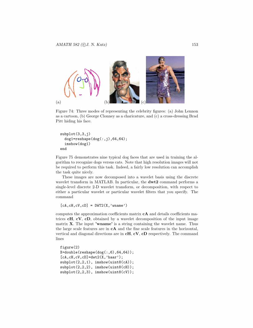
AMATH 582 ( c©J. N. Kutz) 153
(a) (b) (c)
Figure 74: Three modes of representing the celebrity figures: (a) John Lennonas a cartoon, (b) George Clonney as a charicature, and (c) a cross-dressing BradPitt hiding his face.
subplot(3,3,j)
dog1=reshape(dog(:,j),64,64);
imshow(dog1)
end
Figure 75 demonstrates nine typical dog faces that are used in training the al-gorithm to recognize dogs versus cats. Note that high resolution images will notbe required to perform this task. Indeed, a fairly low resolution can accomplishthe task quite nicely.
These images are now decomposed into a wavelet basis using the discretewavelet transform in MATLAB. In particular, the dwt2 command performs asingle-level discrete 2-D wavelet transform, or decomposition, with respect toeither a particular wavelet or particular wavelet filters that you specify. Thecommand
[cA,cH,cV,cD] = DWT2(X,’wname’)
computes the approximation coefficients matrix cA and details coefficients ma-trices cH, cV, cD, obtained by a wavelet decomposition of the input imagematrix X. The input ’wname’ is a string containing the wavelet name. Thusthe large scale features are in cA and the fine scale features in the horizontal,vertical and diagonal directions are in cH, cV, cD respectively. The commandlines
figure(2)
X=double(reshape(dog(:,6),64,64));
[cA,cH,cV,cD]=dwt2(X,’haar’);
subplot(2,2,1), imshow(uint8(cA));
subplot(2,2,2), imshow(uint8(cH));
subplot(2,2,3), imshow(uint8(cV));
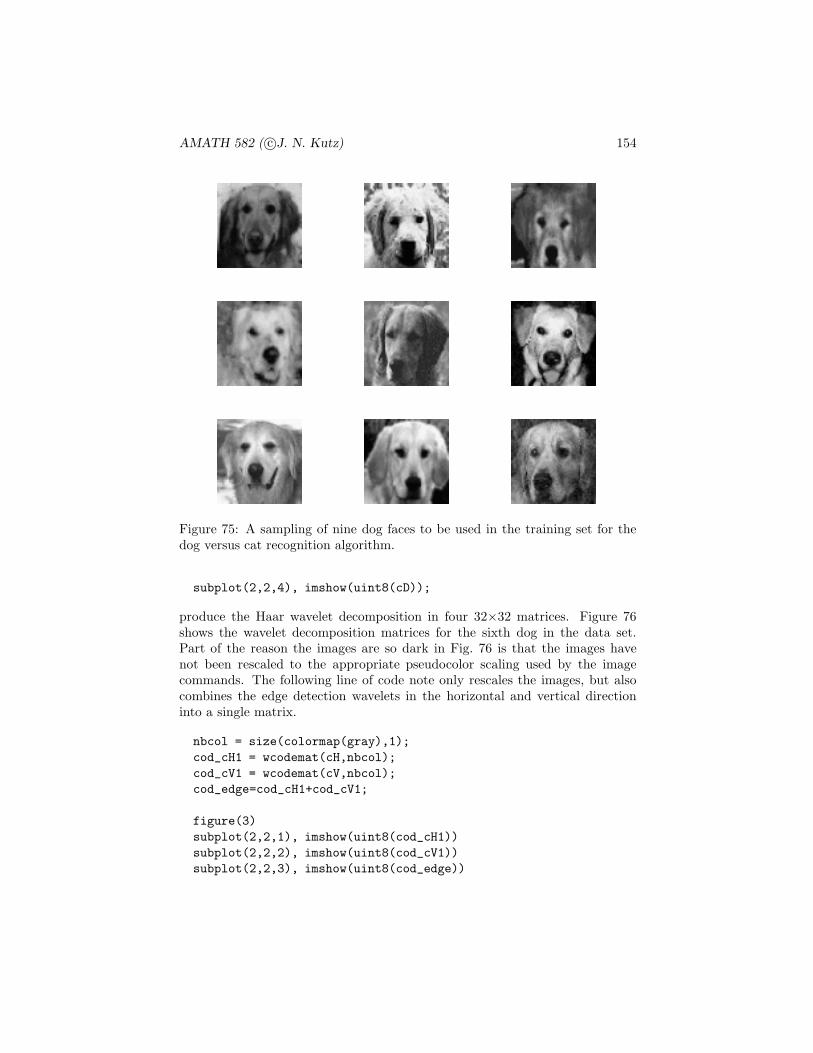
AMATH 582 ( c©J. N. Kutz) 154
Figure 75: A sampling of nine dog faces to be used in the training set for thedog versus cat recognition algorithm.
subplot(2,2,4), imshow(uint8(cD));
produce the Haar wavelet decomposition in four 32×32 matrices. Figure 76shows the wavelet decomposition matrices for the sixth dog in the data set.Part of the reason the images are so dark in Fig. 76 is that the images havenot been rescaled to the appropriate pseudocolor scaling used by the imagecommands. The following line of code note only rescales the images, but alsocombines the edge detection wavelets in the horizontal and vertical directioninto a single matrix.
nbcol = size(colormap(gray),1);
cod_cH1 = wcodemat(cH,nbcol);
cod_cV1 = wcodemat(cV,nbcol);
cod_edge=cod_cH1+cod_cV1;
figure(3)
subplot(2,2,1), imshow(uint8(cod_cH1))
subplot(2,2,2), imshow(uint8(cod_cV1))
subplot(2,2,3), imshow(uint8(cod_edge))
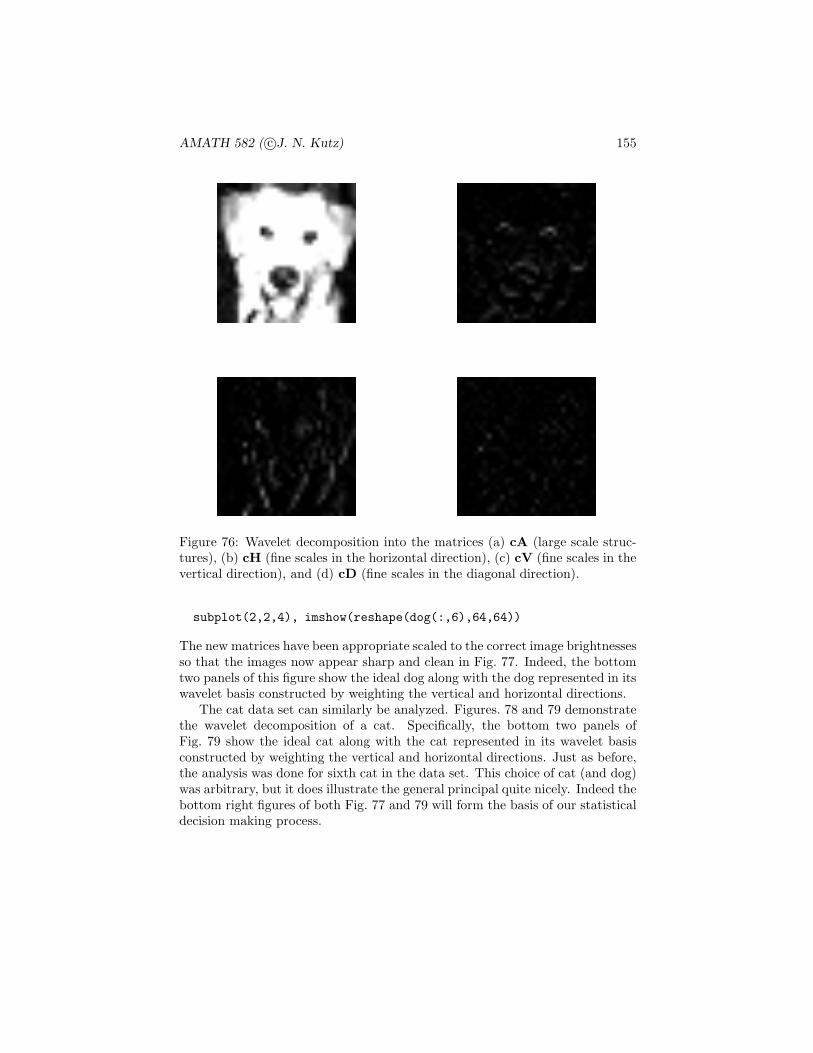
AMATH 582 ( c©J. N. Kutz) 155
Figure 76: Wavelet decomposition into the matrices (a) cA (large scale struc-tures), (b) cH (fine scales in the horizontal direction), (c) cV (fine scales in thevertical direction), and (d) cD (fine scales in the diagonal direction).
subplot(2,2,4), imshow(reshape(dog(:,6),64,64))
The new matrices have been appropriate scaled to the correct image brightnessesso that the images now appear sharp and clean in Fig. 77. Indeed, the bottomtwo panels of this figure show the ideal dog along with the dog represented in itswavelet basis constructed by weighting the vertical and horizontal directions.
The cat data set can similarly be analyzed. Figures. 78 and 79 demonstratethe wavelet decomposition of a cat. Specifically, the bottom two panels ofFig. 79 show the ideal cat along with the cat represented in its wavelet basisconstructed by weighting the vertical and horizontal directions. Just as before,the analysis was done for sixth cat in the data set. This choice of cat (and dog)was arbitrary, but it does illustrate the general principal quite nicely. Indeed thebottom right figures of both Fig. 77 and 79 will form the basis of our statisticaldecision making process.
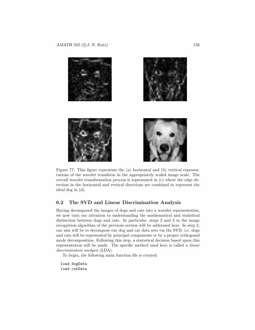
AMATH 582 ( c©J. N. Kutz) 156
Figure 77: This figure represents the (a) horizontal and (b) vertical represen-tations of the wavelet transform in the appropriately scaled image scale. Theoverall wavelet transformation process is represented in (c) where the edge de-tection in the horizontal and vertical directions are combined to represent theideal dog in (d).
6.2 The SVD and Linear Discrimination Analysis
Having decomposed the images of dogs and cats into a wavelet representation,we now turn our attention to understanding the mathematical and statisticaldistinction between dogs and cats. In particular, steps 2 and 3 in the imagerecognition algorithm of the previous section will be addressed here. In step 2,our aim will be to decompose our dog and cat data sets via the SVD, i.e. dogsand cats will be represented by principal components or by a proper orthogonalmode decomposition. Following this step, a statistical decision based upon thisrepresentation will be made. The specific method used here is called a lineardiscrimination analysis (LDA).
To begin, the following main function file is created:
load dogData
load catData
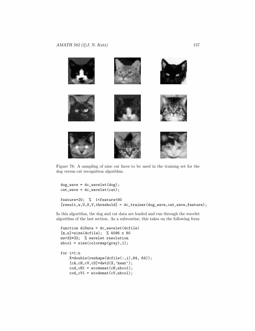
AMATH 582 ( c©J. N. Kutz) 157
Figure 78: A sampling of nine cat faces to be used in the training set for thedog versus cat recognition algorithm.
dog_wave = dc_wavelet(dog);
cat_wave = dc_wavelet(cat);
feature=20; % 1<feature<80
[result,w,U,S,V,threshold] = dc_trainer(dog_wave,cat_wave,feature);
In this algorithm, the dog and cat data are loaded and run through the waveletalgorithm of the last section. As a subroutine, this takes on the following form
function dcData = dc_wavelet(dcfile)
[m,n]=size(dcfile); % 4096 x 80
nw=32*32; % wavelet resolution
nbcol = size(colormap(gray),1);
for i=1:n
X=double(reshape(dcfile(:,i),64, 64));
[cA,cH,cV,cD]=dwt2(X,’haar’);
cod_cH1 = wcodemat(cH,nbcol);
cod_cV1 = wcodemat(cV,nbcol);

AMATH 582 ( c©J. N. Kutz) 158
Figure 79: This figure represents the (a) horizontal and (b) vertical represen-tations of the wavelet transform in the appropriately scaled image scale. Theoverall wavelet transformation process is represented in (c) where the edge de-tection in the horizontal and vertical directions are combined to represent theideal dog in (d).
cod_edge=cod_cH1+cod_cV1;
dcData(:,i)=reshape(cod_edge,nw,1);
end
where is should be recalled that the cA, cH, cV and cD are the wavelet decom-positions with a resolution of 32×32. Upon generating this data, the subroutinedc trainer.m is called. This subroutine will perform and SVD and LDA in or-der to train itself to recognize dogs and cats. The variable feature determinesthe number of principal components that will be used to classify the dog andcat features.
The SVD decomposition
The first step in setting up the statistical analysis is the SVD decompositionof the wavelet generated data. The subroutine dc trainer.m accepts as input

AMATH 582 ( c©J. N. Kutz) 159
the wavelet decomposed dog and cat data along with the number of PCA/PODcomponents to be considered with the variable feature. Upon entry into thesubroutine, the dog and cat data are concatenated and the SVD is performed.The following code performs with the reduced SVD to extract the key compo-nents U, Σ and V.
function [result,w,U,S,V,th]=dc_trainer(dog0,cat0,feature)
nd=length(dog0(1,:)); nc=length(cat0(1,:));
[U,S,V] = svd([dog0,cat0],0); % reduced SVD
animals = S*V’;
U = U(:,1:feature);
dogs = animals(1:feature,1:nd);
cats = animals(1:feature,nd+1:nd+nc);
Recall that only a limited number of the principal components are consideredin the feature detection as determined by the variable feature. Thus uponcompletion of the SVD step, a limited number of columns of U and rows ofΣV∗ are extracted. Further, new variables cats and dogs are generated givingthe strength of the cat and dog projections on the PCA/POD modes generatedby U.
To get a better feeling of what has just happened, the SVD matrices U, Σand V are all returned in the subroutine to the main file. In the main file, thedecomposition can be visualized. What is of most interest is the PCA/PODthat is generated from the cat and dog data. This can be reconstructed withthe following code
for j=1:4
subplot(2,2,j)
ut1=reshape(U(:,j),32,32);
ut2=ut1(32:-1:1,:);
pcolor(ut2)
set(gca,’Xtick’,[],’Ytick’,[])
end
Thus the first four columns, or PCA/POD modes, are plotted by reshaping themback into 32×32 images. Figure 80 shows the first four POD modes associatedwith the dog and cat data. The strength of each of these modes in a given cator dog can be computed by the projection onto ΣV∗. In particular, the singular(diagonal) elements of Σ gives the strength of the projection of each cat ontothe POD modes. Figures 81 and 82 demonstrate the singular values associatedwith the cat and dog data along with the strength of each cat projected onto thePOD modes. These two plots are created from the main file with the commands
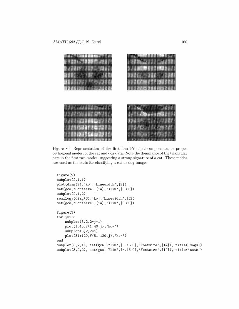
AMATH 582 ( c©J. N. Kutz) 160
Figure 80: Representation of the first four Principal components, or properorthogonal modes, of the cat and dog data. Note the dominance of the triangularears in the first two modes, suggesting a strong signature of a cat. These modesare used as the basis for classifying a cat or dog image.
figure(2)
subplot(2,1,1)
plot(diag(S),’ko’,’Linewidth’,[2])
set(gca,’Fontsize’,[14],’Xlim’,[0 80])
subplot(2,1,2)
semilogy(diag(S),’ko’,’Linewidth’,[2])
set(gca,’Fontsize’,[14],’Xlim’,[0 80])
figure(3)
for j=1:3
subplot(3,2,2*j-1)
plot(1:40,V(1:40,j),’ko-’)
subplot(3,2,2*j)
plot(81:120,V(81:120,j),’ko-’)
end
subplot(3,2,1), set(gca,’Ylim’,[-.15 0],’Fontsize’,[14]), title(’dogs’)
subplot(3,2,2), set(gca,’Ylim’,[-.15 0],’Fontsize’,[14]), title(’cats’)
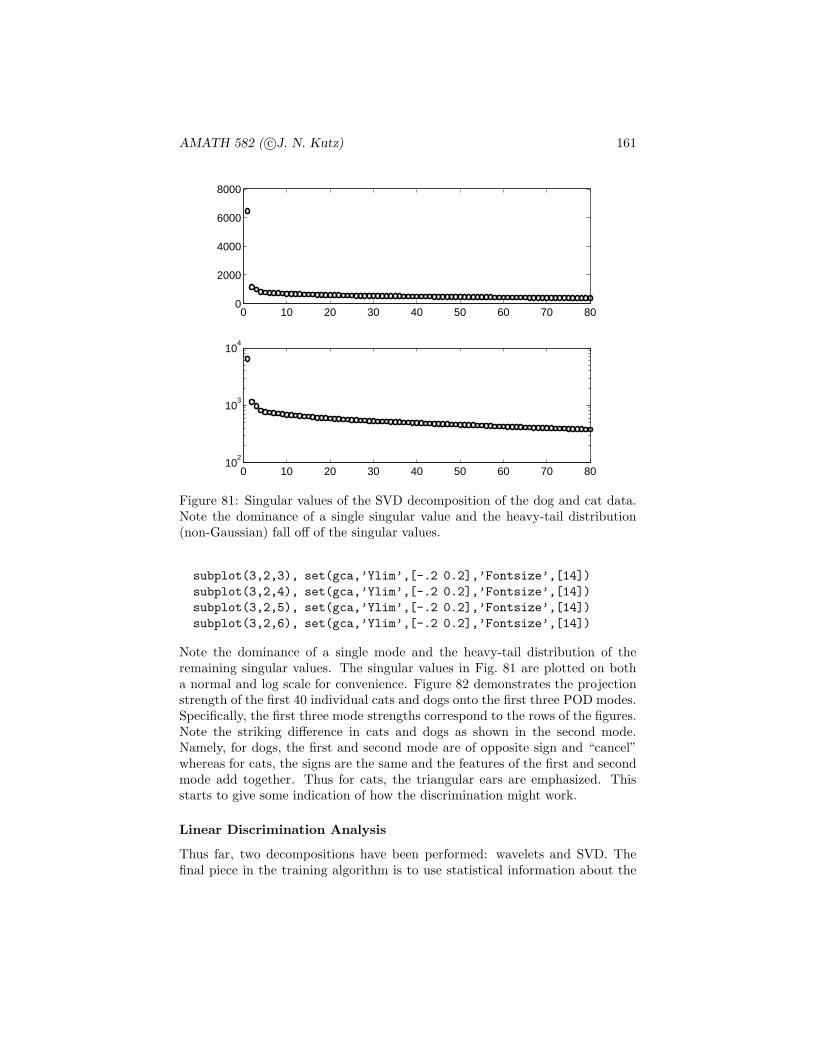
AMATH 582 ( c©J. N. Kutz) 161
0 10 20 30 40 50 60 70 800
2000
4000
6000
8000
0 10 20 30 40 50 60 70 8010
2
103
104
Figure 81: Singular values of the SVD decomposition of the dog and cat data.Note the dominance of a single singular value and the heavy-tail distribution(non-Gaussian) fall off of the singular values.
subplot(3,2,3), set(gca,’Ylim’,[-.2 0.2],’Fontsize’,[14])
subplot(3,2,4), set(gca,’Ylim’,[-.2 0.2],’Fontsize’,[14])
subplot(3,2,5), set(gca,’Ylim’,[-.2 0.2],’Fontsize’,[14])
subplot(3,2,6), set(gca,’Ylim’,[-.2 0.2],’Fontsize’,[14])
Note the dominance of a single mode and the heavy-tail distribution of theremaining singular values. The singular values in Fig. 81 are plotted on botha normal and log scale for convenience. Figure 82 demonstrates the projectionstrength of the first 40 individual cats and dogs onto the first three POD modes.Specifically, the first three mode strengths correspond to the rows of the figures.Note the striking difference in cats and dogs as shown in the second mode.Namely, for dogs, the first and second mode are of opposite sign and “cancel”whereas for cats, the signs are the same and the features of the first and secondmode add together. Thus for cats, the triangular ears are emphasized. Thisstarts to give some indication of how the discrimination might work.
Linear Discrimination Analysis
Thus far, two decompositions have been performed: wavelets and SVD. Thefinal piece in the training algorithm is to use statistical information about the

AMATH 582 ( c©J. N. Kutz) 162
0 10 20 30 40
−0.1
−0.05
0dogs
80 90 100 110 120
−0.1
−0.05
0cats
0 10 20 30 40−0.2
0
0.2
80 90 100 110 120−0.2
0
0.2
0 10 20 30 40−0.2
0
0.2
80 90 100 110 120−0.2
0
0.2
Figure 82: Projection of the first 40 individual cats and dogs onto the first threePOD modes as described by the SVD matrix V. The left column is the first 40dogs while the right column is the first 40 cats. The three rows of figures arethe projections on to the first three POD modes.
wavelet/SVD decomposition in order to make a decision about wether the imageis indeed a dog or cat. Figure 83 gives a cartoon of the key idea involved inthe LDA. The idea of the LDA was first proposed by Fisher [21] in the contextof taxonomy. In our example, two data sets are considered and projected ontonew bases. In the left figure, the projection shows the data to be completelymixed, not allowing for any reasonable way to separate the data from eachother. In the right figure, which is the ideal charicature for LDA, the data arewell separated with the means µ1 and µ2 being well apart when projected ontothe chosen subspace. Thus the goal of LDA is two-fold: find a suitable projectionthat maximizes the distance between the inter-class data while minimizing theintra-class data.
For a two-class LDA, the above idea results in consideration of the followingmathematical formulation. Construct a projection w such that
w = argmaxw
wTSBw
wTSWw(6.2.152)
where the scatter matrices for between-class SB and within-class SW data are
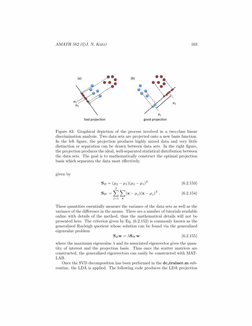
AMATH 582 ( c©J. N. Kutz) 163
!"#$$ !%#$$
&'$$
&($$&'$$ &($$
%")$*+,-./0,1$ 2,,)$*+,-./0,1$
Figure 83: Graphical depiction of the process involved in a two-class lineardiscrimination analysis. Two data sets are projected onto a new basis function.In the left figure, the projection produces highly mixed data and very littledistinction or separation can be drawn between data sets. In the right figure,the projection produces the ideal, well-separated statistical distribution betweenthe data sets. The goal is to mathematically construct the optimal projectionbasis which separates the data most effectively.
given by
SB = (µ2 − µ1)(µ2 − µ1)T (6.2.153)
SW =
2∑
j=1
∑
x
(x − µj)(x − µj)T . (6.2.154)
These quantities essentially measure the variance of the data sets as well as thevariance of the difference in the means. There are a number of tutorials availableonline with details of the method, thus the mathematical details will not bepresented here. The criterion given by Eq. (6.2.152) is commonly known as thegeneralized Rayleigh quotient whose solution can be found via the generalizedeigenvalue problem
SBw = λSWw (6.2.155)
where the maximum eigenvalue λ and its associated eigenvector gives the quan-tity of interest and the projection basis. Thus once the scatter matrices areconstructed, the generalized eigenvectors can easily be constructed with MAT-LAB.
Once the SVD decomposition has been performed in the dc trainer.m sub-routine, the LDA is applied. The following code produces the LDA projection
AMATH 582 ( c©J. N. Kutz) 164
basis as well as the decision threshold level associated with the dog and catrecognition.
md = mean(dogs,2);
mc = mean(cats,2);
Sw=0; % within class variances
for i=1:nd
Sw = Sw + (dogs(:,i)-md)*(dogs(:,i)-md)’;
end
for i=1:nc
Sw = Sw + (cats(:,i)-mc)*(cats(:,i)-mc)’;
end
Sb = (md-mc)*(md-mc)’; % between class
[V2,D] = eig(Sb,Sw); % linear discriminant analysis
[lambda,ind] = max(abs(diag(D)));
w = V2(:,ind); w = w/norm(w,2);
vdog = w’*dogs; vcat = w’*cats;
result = [vdog,vcat];
if mean(vdog)>mean(vcat)
w = -w;
vdog = -vdog;
vcat = -vcat;
end
% dog < threshold < cat
sortdog = sort(vdog);
sortcat = sort(vcat);
t1 = length(sortdog);
t2 = 1;
while sortdog(t1)>sortcat(t2)
t1 = t1-1;
t2 = t2+1;
end
threshold = (sortdog(t1)+sortcat(t2))/2;
This code ends the subroutine dc trainer.m since the statistical threshold levelhas been determined along with the appropriate LDA basis for projecting a newimage of a dog or cat. For feature=20 as carried through the codes presentedhere, a histogram can be constructed of the dog and cat statistics.
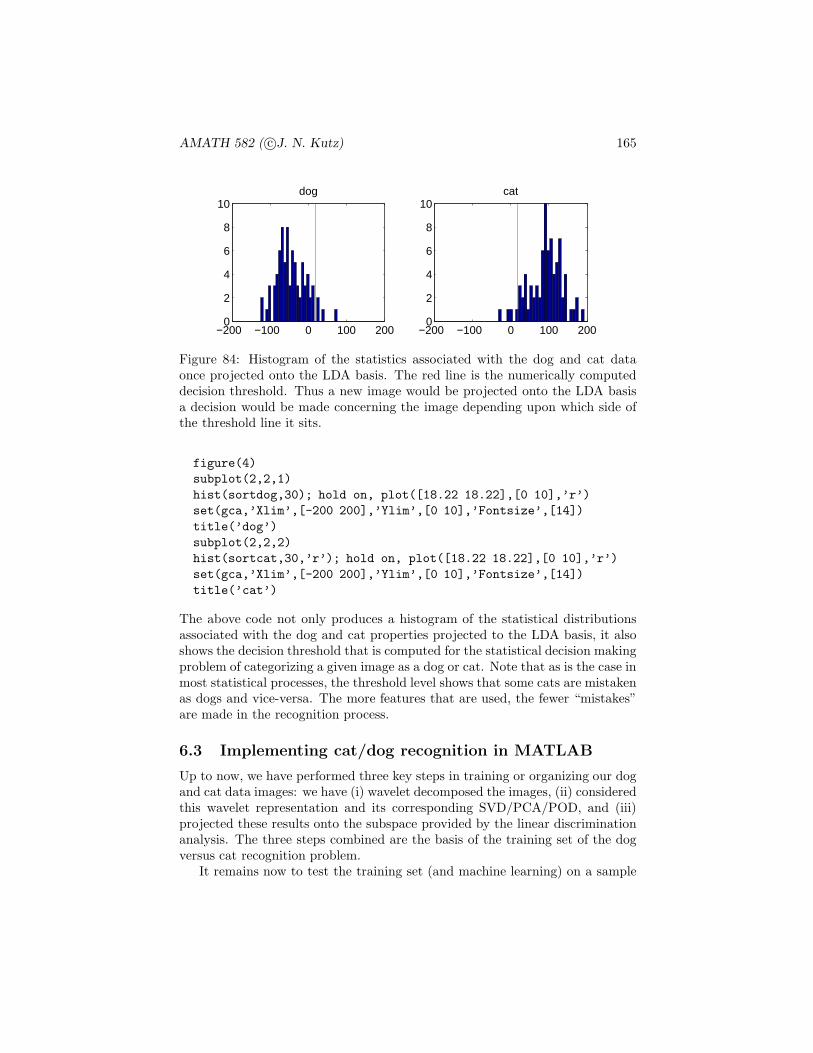
AMATH 582 ( c©J. N. Kutz) 165
−200 −100 0 100 2000
2
4
6
8
10dog
−200 −100 0 100 2000
2
4
6
8
10cat
Figure 84: Histogram of the statistics associated with the dog and cat dataonce projected onto the LDA basis. The red line is the numerically computeddecision threshold. Thus a new image would be projected onto the LDA basisa decision would be made concerning the image depending upon which side ofthe threshold line it sits.
figure(4)
subplot(2,2,1)
hist(sortdog,30); hold on, plot([18.22 18.22],[0 10],’r’)
set(gca,’Xlim’,[-200 200],’Ylim’,[0 10],’Fontsize’,[14])
title(’dog’)
subplot(2,2,2)
hist(sortcat,30,’r’); hold on, plot([18.22 18.22],[0 10],’r’)
set(gca,’Xlim’,[-200 200],’Ylim’,[0 10],’Fontsize’,[14])
title(’cat’)
The above code not only produces a histogram of the statistical distributionsassociated with the dog and cat properties projected to the LDA basis, it alsoshows the decision threshold that is computed for the statistical decision makingproblem of categorizing a given image as a dog or cat. Note that as is the case inmost statistical processes, the threshold level shows that some cats are mistakenas dogs and vice-versa. The more features that are used, the fewer “mistakes”are made in the recognition process.
6.3 Implementing cat/dog recognition in MATLAB
Up to now, we have performed three key steps in training or organizing our dogand cat data images: we have (i) wavelet decomposed the images, (ii) consideredthis wavelet representation and its corresponding SVD/PCA/POD, and (iii)projected these results onto the subspace provided by the linear discriminationanalysis. The three steps combined are the basis of the training set of the dogversus cat recognition problem.
It remains now to test the training set (and machine learning) on a sample
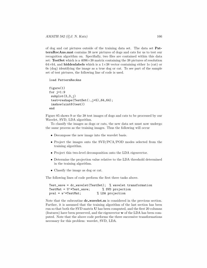
AMATH 582 ( c©J. N. Kutz) 166
of dog and cat pictures outside of the training data set. The data set Pat-ternRecAns.mat contains 38 new pictures of dogs and cats for us to test ourrecognition algorithm on. Specifially, two files are contained within this dataset: TestSet which is a 4096×38 matrix containing the 38 pictures of resolution64×64, and hiddenlabels which is a 1×38 vector containing either 1s (cat) or0s (dog) identifying the image as a true dog or cat. To see part of the sampleset of test pictures, the following line of code is used.
load PatternRecAns
figure(1)
for j=1:9
subplot(3,3,j)
test=reshape(TestSet(:,j+5),64,64);
imshow(uint8(test))
end
Figure 85 shows 9 or the 38 test images of dogs and cats to be processed by ourWavelet, SVD, LDA algorithm.
To classify the images as dogs or cats, the new data set must now undergothe same process as the training images. Thus the following will occur
• Decompose the new image into the wavelet basis.
• Project the images onto the SVD/PCA/POD modes selected from thetraining algorithm.
• Project this two-level decomposition onto the LDA eigenvector.
• Determine the projection value relative to the LDA threshold determinedin the training algorithm.
• Classify the image as dog or cat.
The following lines of code perform the first three tasks above.
Test_wave = dc_wavelet(TestSet); % wavelet transformation
TestMat = U’*Test_wave; % SVD projection
pval = w’*TestMat; % LDA projection
Note that the subroutine dc wavelet.m is considered in the previous section.Further, it is assumed that the training algorithm of the last section has beenrun so that both the SVD matrix U has been computed, and the first 20 columns(features) have been preserved, and the eigenvector w of the LDA has been com-puted. Note that the above code performs the three successive transformationsnecessary for this problem: wavelet, SVD, LDA.
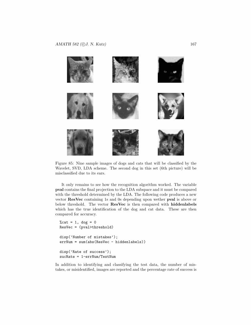
AMATH 582 ( c©J. N. Kutz) 167
Figure 85: Nine sample images of dogs and cats that will be classified by theWavelet, SVD, LDA scheme. The second dog in this set (6th picture) will bemisclassified due to its ears.
It only remains to see how the recognition algorithm worked. The variablepval contains the final projection to the LDA subspace and it must be comparedwith the threshold determined by the LDA. The following code produces a newvector ResVec containing 1s and 0s depending upon wether pval is above orbelow threshold. The vector ResVec is then compared with hiddenlabelswhich has the true identification of the dog and cat data. These are thencompared for accuracy.
%cat = 1, dog = 0
ResVec = (pval>threshold)
disp(’Number of mistakes’);
errNum = sum(abs(ResVec - hiddenlabels))
disp(’Rate of success’);
sucRate = 1-errNum/TestNum
In addition to identifying and classifying the test data, the number of mis-takes, or misidentified, images are reported and the percentage rate of success is
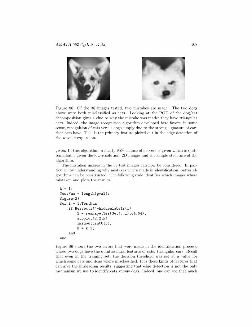
AMATH 582 ( c©J. N. Kutz) 168
Figure 86: Of the 38 images tested, two mistakes are made. The two dogsabove were both misclassified as cats. Looking at the POD of the dog/catdecomposition gives a clue to why the mistake was made: they have triangularears. Indeed, the image recognition algorithm developed here favors, in somesense, recognition of cats versus dogs simply due to the strong signature of earsthat cats have. This is the primary feature picked out in the edge detection ofthe wavelet expansion.
given. In this algorithm, a nearly 95% chance of success is given which is quiteremarkable given the low-resolution, 2D images and the simple structure of thealgorithm.
The mistaken images in the 38 test images can now be considered. In par-ticular, by understanding why mistakes where made in identification, better al-gorithms can be constructed. The following code identifies which images wheremistaken and plots the results.
k = 1;
TestNum = length(pval);
figure(2)
for i = 1:TestNum
if ResVec(i)~=hiddenlabels(i)
S = reshape(TestSet(:,i),64,64);
subplot(2,2,k)
imshow(uint8(S))
k = k+1;
end
end
Figure 86 shows the two errors that were made in the identification process.These two dogs have the quintessential features of cats: triangular ears. Recallthat even in the training set, the decision threshold was set at a value forwhich some cats and dogs where misclassified. It is these kinds of features thatcan give the misleading results, suggesting that edge detection is not the onlymechanism we use to identify cats versus dogs. Indeed, one can see that much

AMATH 582 ( c©J. N. Kutz) 169
more sophisticated algorithms could be used based upon size of the animal,color, coat pattern, walking cadence, etc. Of course, the more sophisticated thealgorithm, the more computationally expensive. This is a fast, low-resolutionroutine that produces 95% accuracy and can be easily implemented.
7 Dimensionality Reduction for Partial Differ-ential Equations
One of the most important uses of computational methods and techniques isin its applications to modeling of physical, engineering, or biological systemsthat demonstrate spatio-temporal dynamics and patterns. For instance, thefield of fluid dynamics fundamentally revolves around being able to predictthe time and space dynamics of a fluid through some, potentially complicatedgeometry. Understanding the interplay of spatial patterns in time indeed isoften the central focus of the field of partial differential equations. In systemswhere the underlying spatial patterns exhibit low-dimensional (pattern forming)dynamics, then the application of the proper orthogonal decomposition can playa critical role in predicting the resulting low-dimensional dynamics.
7.1 Modal expansion techniques for PDEs
Partial differential equations (PDEs) are fundamental to the understanding ofthe underlying physics, biophysics, etc. of complex dynamical systems. In par-ticular, a partial differential equation gives the governing evolution of a systemin both time and space. Abstractly, this can be represented by the followingPDE system:
Ut = N(U,Ux,Uxx, · · · , x, t) (7.1.156)
where U is a vector of physically relevant quantities and the subscripts t andx denote partial differentiation. The function N(·) captures the space-timedynamics that is specific to the system being considered. Along with this PDEare some prescribed boundary conditions and initial conditions. In general, thiscan be a complicated, nonlinear function of the quantity U, its derivatives andboth space and time.
In general, there are no techniques for building analytic solutions for (7.1.156).However for specific forms of N(·), such as the case where the function is linearin U, time-indenpendent and constant coefficient, then standard PDE solutiontechniques may be used to characterize the dynamics analytically. Such solutionmethods are the core of typical PDE courses at both the graduate and under-graduate level. The specific process for solving PDE systems is illustrated inFig. 87 where a reduction from a PDE to ODE is first performed and then areduction from an ODE to algebra is enacted. Provided such reductions can beachieved and undone, then an analytic solution is produced.

AMATH 582 ( c©J. N. Kutz) 170
Figure 87: Basic solution technique for solving a partial differential equation.The first step is to reduce it to an appropriate set of ordinary differential equa-tions and then algebra. If the reduction can be undone, then a complete analyticsolution can be produced. The starred quantity, i.e. algebra, is the goal of anyPDE or ODE reduction.
To be more specific about the solution method concept in Fig. 87, a numberof standard solution techniques can be discussed. The first to be highlightedis the technique of self-similarity reduction. This method simply attempts toextract a fundamental relationship between time and space by making a changeof variable to, for instance, a new variable such as
ξ = xβtα (7.1.157)
where β and α are determined by making the change of variable in (7.1.156).This effectively performs the first step in the reduction process by reducingthe PDE to an ODE in the variable ξ alone. A second, and perhaps the mostcommon introductory technique, is the method of separation of variables wherethe assumption
U(x, t) = F(x)G(t) (7.1.158)
is made. Thus effectively separating time and space in the solution. Whenapplied to (7.1.156) with N(·) being linear in U, two ODEs result: one for thetime dynamics G(t) and one for the spatial dynamics F(x). If the function N(·)is nonlinear in U, then separation cannot be achieved.
As a specific example of the application of the method of separation, weconsider here the eigenfunction expansion technique. Strictly speaking, to makeanalytic progress with the method of separation of variables, one must requirethat separation occurs. However, no such requirement needs to be made if weare simply using the method as the basis of a computational technique. Inparticular, the eigenfunction expansion techniques assumes a solution of theform
u(x, t) =
∞∑
n=1
an(t)φn(x) (7.1.159)
AMATH 582 ( c©J. N. Kutz) 171
where the φn(x) are an orthogonal set of eigenfunctions and we have assumedthat the PDE is now described by a scalar quantity u(x, t). The φn(x) can beany orthogonal set of functions such that
(φj(x), φk(x)) = δjk =
{1 j = k0 j 6= q
(7.1.160)
where δjk is the Dirac function and the notation (φj , φk) =∫φjφ
∗kdx gives the
inner product. For a given physical problem, one may be motivated to usea specified set of eigenfunctions such as those special functions that arise forspecific geometries or symmetries. More generally, for computational purposes,it is desired to use a set of eigenfunctions that produce accurate and rapidevaluation of the solutions of (7.1.156). Two eigenfunctions immediately cometo mind: the Fourier modes and Chebyshev polynomials. This is largely in partdue to their spectral accuracy properties and tremendous speed advantages suchas O(N logN) speed in projection to the spectral basis.
To give a specific demonstration of this technique, consider the nonlinearSchrodinger (NLS) equation
iut +1
2uxx + |u|2u = 0 (7.1.161)
with the boundary conditions u→ 0 as x→ ±∞. If not for the nonlinear term,this equation could be solved easily in closed form. However, the nonlinearitymixes the eigenfunction components in the expansion (7.1.159) making a simpleanalytic solution not possible.
To solve the NLS computationally, a Fourier mode expansion is used. Thususe can be made of the standard fast Fourier transform. The following codeformulates the PDE solution as an eigenfunction expansion technique (7.1.159)of the NLS (7.1.161). The first step in the process is to define an appropriatespatial and time domain for the solution along with the Fourier frequenciespresent in the system. The following code produces both the time and spacedomain of interest:
% space
L=40; n=512;
x2=linspace(-L/2,L/2,n+1); x=x2(1:n);
k=(2*pi/L)*[0:n/2-1 -n/2:-1].’;
% time
t=0:0.1:10;
It now remains to consider a specific spatial configuration for the initialcondition. For the NLS, there are a set of special initial conditions called solitonswhere the initial conditions are given by
u(x, 0) = Nsech(x) (7.1.162)

AMATH 582 ( c©J. N. Kutz) 172
−200
20
03
60
1
xt
|u|
−400
40
03
60
40
kt
|fft(
u)|
Figure 88: Evolution of the N = 1 soliton. Although it appears to be a verysimple evolution, the phase is evolving in a nonlinear fashion and approximately50 Fourier modes are required to model accurately this behavior.
−200
20
03
60
4
xt
|u|
−400
40
03
60
80
kt
|fft(
u)|
Figure 89: Evolution of the N = 2 soliton. Here a periodic dynamics is observedand approximately 200 Fourier modes are required to model accurately thebehavior.
where N is an integer. We will consider the soliton dynamics with N = 1 andN = 2 respectively. In order to do so, the initial condition is projected ontothe Fourier modes with the fast Fourier transform. Rewriting (7.1.161) in theFourier domain, i.e. Fourier transforming, gives the set of differential equations
ut = − i
2k2u+ i ˆ|u|2u (7.1.163)
where the Fourier mode mixing occurs due to the nonlinear mixing in the cubicterm. This gives the system of differential equations to be solved for in orderto evaluate the NLS behavior. The following code solves the set of differentialequations in the Fourier domain.
% initial conditions
N=1;
u=N*sech(x);
ut=fft(u);
[t,utsol]=ode45(’nls_rhs’,t,ut,[],k);

AMATH 582 ( c©J. N. Kutz) 173
0 10 20 300
10
20
30
σ j
0 10 20 30
10−6
10−3
100
103
log(
σ j)
−15 0 15−0.2
0
0.2
x
φ j(x)
mode1mode2
Figure 90: Projection of the N = 1 evolution to POD modes. The top twofigures are the singular values σj of the evolution demonstrated in (88) on both aregular scale and log scale. This demonstrates that the N = 1 soliton dynamicsis primarily a single mode dynamics. The first two modes are shown in thebottom panel. Indeed, the second mode is meaningless and is generated fromnoise and numerical round-off.
for j=1:length(t)
usol(j,:)=ifft(utsol(j,:)); % bring back to space
end
subplot(2,2,1), waterfall(x,t,abs(usol)), colormap([0 0 0])
subplot(2,2,2), waterfall(fftshift(k),t,abs(fftshift(utsol)))
In the solution code, the following right hand side function nls rhs.m is calledthat effectively produces the differential equation (7.1.163):
function rhs=nls_rhs(t,ut,dummy,k)
u=ifft(ut);
rhs=-(i/2)*(k.^2).*ut+i*fft( (abs(u).^2).*u );
This gives a complete code that produces both the time-space evolution and thetime-frequency evolution.
The dynamics of the N = 1 and N = 2 solitons are demonstrated in Figs. 88and 89 respectively. During evolution, the N = 1 soliton only undergoes phase
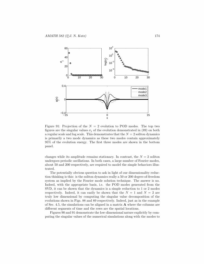
AMATH 582 ( c©J. N. Kutz) 174
0 10 20 300
20
40
60
σ j
0 10 20 30
10−6
10−3
100
103
log(
σ j)
−15 0 15−0.4
0
0.4
x
φ j(x)
mode1mode2mode3
Figure 91: Projection of the N = 2 evolution to POD modes. The top twofigures are the singular values σj of the evolution demonstrated in (89) on botha regular scale and log scale. This demonstrates that theN = 2 soliton dynamicsis primarily a two mode dynamics as these two modes contain approximately95% of the evolution energy. The first three modes are shown in the bottompanel.
changes while its amplitude remains stationary. In contrast, the N = 2 solitonundergoes periodic oscillations. In both cases, a large number of Fourier modes,about 50 and 200 respectively, are required to model the simple behaviors illus-trated.
The potentially obvious question to ask in light of our dimensionality reduc-tion thinking is this: is the soliton dynamics really a 50 or 200 degree-of-freedomsystem as implied by the Fourier mode solution technique. The answer is no.Indeed, with the appropriate basis, i.e. the POD modes generated from theSVD, it can be shown that the dynamics is a simple reduction to 1 or 2 modesrespectively. Indeed, it can easily be shown that the N = 1 and N = 2 aretruly low dimensional by computing the singular value decomposition of theevolutions shown in Figs. 88 and 89 respectively. Indeed, just as in the exampleof Sec. 4.5, the simulations can be aligned in a matrix A where the columns aredifferent segments of time and the rows are the spatial locations.
Figures 90 and 91 demonstrate the low-dimensional nature explicitly by com-puting the singular values of the numerical simulations along with the modes to

AMATH 582 ( c©J. N. Kutz) 175
be used in our new eigenfunction expansion. What is clear is that for both ofthese cases, the dynamics is truly low dimensional with the N = 1 soliton beingmodeled exceptionally well by a single POD mode while the N = 2 dynamicsis modeled quite well with two POD modes. Thus in performing the expansion(7.1.159), the modes chosen should be the POD modes generated from the simu-lations themselves. In the next section, we will derive the dynamics of the modalinteraction for these two cases and show that quite a bit of analytic progresscan then be made within the POD framework.
7.2 PDE dynamics in the right (best) basis
The last section demonstrated the N = 1 and N = 2 soliton dynamics of theNLS equation (7.1.161). In particular, Figs. 88 and 89 showed the evolutiondynamics in the Fourier mode basis that was used in the computation of theevolution. The primary motivation in performing a POD reduction of the dy-namics through (7.1.159) is the observation in Figs. 90 and 91 that both dynam-ics are truly low-dimensional with only one or two modes playing a dominantrole respectively.
N = 1 Soliton Reduction
Two take advantage of the low dimensional structure, we first consider theN = 1 soliton dynamics. Figure 88 shows that a single mode in the SVDdominates the dynamics. This is the first column of the U matrix (see Sec. 4.5).Thus the dynamics is recast in a single mode so that
u(x, t) = a(t)φ(x) (7.2.164)
where now there is now sum in (7.1.159) since there is only a single mode φ(x).Plugging in this equation into the NLS equation (7.1.161) yields the following:
iatφ+1
2aφxx + |a|2a|φ|2φ = 0 . (7.2.165)
The inner product is now taken with respect to φ which gives
iat +α
2a+ β|a|2a = 0 (7.2.166)
where
α =(φxx, φ)
(φ, φ)(7.2.167a)
β =(|φ|2φ, φ)
(φ, φ)(7.2.167b)

AMATH 582 ( c©J. N. Kutz) 176
−200
20
03
60
1
xt
|u|
−200
20
03
60
1
xt
|u|
0 3 60
1
2
3
t
phas
e
(a) (b)
PDEPOD analytic
Figure 92: Comparison of (a) full PDE dynamics and (b) one-mode POD dy-namics. In the bottom figure, the phase of the pulse evolution at x = 0 is plottedfor the full PDE simulations and the one-mode analytic formula (circles) givenin (7.2.171).
and the inner product is defined as integration over the computational intervalso that (φ, ψ) =
∫φψ∗dx. Note that the integration is over the computational
domain and the ∗ denotes the complex conjugate.The differential equation for a(t) given by (7.2.166) can be solved explicitly
to yield
a(t) = a(0) exp[iα
2t+ β|a(0)|2t
](7.2.168)
where a(0) is the initial value condition for a(t). To find the initial condition,recall that
u(x, 0) = sech(x) = a(0)φ(x) . (7.2.169)
Taking the inner product with respect to φ(x) gives
a(0) =(sech(x), φ)
(φ, φ). (7.2.170)
Thus the one mode expansion gives the approximate PDE solution
u(x, t) = a(0) exp[iα
2t+ β|a(0)|2t
]φ(x) . (7.2.171)

AMATH 582 ( c©J. N. Kutz) 177
This solution is the low-dimensional POD approximation of the PDE expandedin the best basis possible, i.e. the SVD determined basis.
For the N = 1 soliton, the spatial profile remains constant while its phaseundergoes a nonlinear rotation. The POD solution (7.2.171) can be solvedexactly to give a characterization of this phase rotation. Figure 92 shows boththe full PDE dynamics along with its one-mode approximation. In this example,the parameters α, β and a(0) were computed using the following code:
% one soliton match
phi_xx=ifft(-(k.^2).*fft(U(:,1)));
norm=trapz(x,U(:,1).*conj(U(:,1)));
A0=trapz(x,(sech(x).’).*conj(U(:,1)))/norm;
alpha=trapz(x,U(:,1).*phi_xx)/norm;
beta=trapz(x,(U(:,1).*conj(U(:,1))).^2)/norm;
This suggest that the N = 1 behavior is indeed a single mode dynamics. Thisis also known to be true from other solution methods, but it is a critical obser-vation that the POD method for PDEs reproduces all of the expected dynamics.
N = 2 Soliton Reduction
The case of the N = 2 soliton is a bit more complicated and interesting.In this case, two modes clearly dominate the behavior of the system. Thesetwo modes are the first two columns of the matrix U and are now used toapproximate the dynamics observed in Fig. (89). In this case, the two modeexpansion takes the form
u(x, t) = a1(t)φ1(x) + a2(t)φ2(x) (7.2.172)
where the φ1 and φ2 are simply taken from the first two columns of the U matrixin the SVD. Inserting this approximation into the governing equation (7.1.161)gives
i (a1tφ1 + a2tφ2) +1
2(a1φ1xx + a2φ2xx) + (a1φ1 + a2φ2)
2(a∗1φ∗1 + a∗2φ
∗2) = 0.
(7.2.173)Multiplying out the cubic term gives the equation
i (a1tφ1 + a2tφ2) +1
2(a1φ1xx + a2φ2xx)
+(|a1|2a1|φ1|2φ1 + |a2|2a2|φ2|2φ2 + 2|a1|2a2|φ1|2φ2 + 2|a2|2a1|φ2|2φ1
+a21a
∗2φ
21φ
∗2 + a2
2a∗1φ
22φ
∗1
). (7.2.174)
All that remains is to take the inner produce of this equation with respect toboth φ1(x) and φ2(x). Recall that these two modes are orthogonal, thus the

AMATH 582 ( c©J. N. Kutz) 178
resulting 2 × 2 system of nonlinear equations results.
ia1t + α11a1 + α12a2 +(β111|a1|2 + 2β211|a2|2
)a1 (7.2.175a)
+(β121|a1|2 + 2β221|a2|2
)a2 + σ121a
21a
∗2 + σ211a
22a
∗1 = 0
ia2t + α21a1 + α22a2 +(β112|a1|2 + 2β212|a2|2
)a1 (7.2.175b)
+(β122|a1|2 + 2β222|a2|2
)a2 + σ122a
21a
∗2 + σ212a
22a
∗1 = 0
where
αjk = (φjxx, φk)/2 (7.2.176a)
βjkl = (|φj |2φk, φl) (7.2.176b)
σjkl = (φ2jφ
∗k, φl) (7.2.176c)
and the initial values of the two components are given by
a1(0) =(2sech(x), φ1)
(φ1, φ1)(7.2.177a)
a2(0) =(2sech(x), φ2)
(φ2, φ2). (7.2.177b)
This gives a complete description of the two mode dynamics predicted from theSVD analysis.
The 2×2 system (7.2.175) can be easily simulated with any standard numer-ical integration algorithm (e.g. fourth-order Runge-Kutta). Before computingthe dynamics, the inner products given by αjk, βjkl and σjkl must be calculatedalong with the initial conditions a1(0) and a2(0). Starting from the code of theprevious section and the SVD decomposition, these quantities can be computedas follows:
% compute the second derivatives
phi_1_xx= ifft( -(k.^2).*fft(U(:,1)) );
phi_2_xx= ifft( -(k.^2).*fft(U(:,2)) );
% compute the norms of the SVD modes
norm1=trapz(x,U(:,1).*conj(U(:,1)));
norm2=trapz(x,U(:,2).*conj(U(:,2)));
% compute the initial conditions
A0_1=trapz(x,(2.0*sech(x).’).*conj(U(:,1)))/norm1;
A0_2=trapz(x,(2.0*sech(x).’).*conj(U(:,2)))/norm2;
% compute inner products alpha, beta, sigma
alpha11=trapz(x,conj(U(:,1)).*phi_1_xx)/norm1;
alpha12=trapz(x,conj(U(:,1)).*phi_2_xx)/norm1;

AMATH 582 ( c©J. N. Kutz) 179
−200
20
01
230
4
xt
|u|
−200
20
01
230
4
xt
|u|
0 1 2 30
8
16
phas
e
(a) (b)
0 1 2 30
5
10
t
mod
es a1
a2
a1
a2
PDEPOD
Figure 93: Comparison of (a) full PDE dynamics and (b) two-mode POD dy-namics. In the bottom two figures, the phase of the pulse evolution at x = 0(middle panel) is plotted for the full PDE simulations and the two-mode dy-namics along with the nonlinear oscillation dynamics of a1(t) and a2(t) (bottompanel).
beta11_1=trapz(x,(U(:,1).*conj(U(:,1))).^2)/norm1;
beta22_1=trapz(x,(U(:,2).*(abs(U(:,2)).^2).*conj(U(:,1))))/norm1;
beta21_1=trapz(x,(U(:,1).*(abs(U(:,2)).^2).*conj(U(:,1))))/norm1;
beta12_1=trapz(x,(U(:,2).*(abs(U(:,1)).^2).*conj(U(:,1))))/norm1;
sigma12_1=trapz(x,(conj(U(:,2)).*(U(:,1).^2).*conj(U(:,1))))/norm1;
sigma21_1=trapz(x,(conj(U(:,1)).*(U(:,2).^2).*conj(U(:,1))))/norm1;
alpha21=trapz(x,conj(U(:,2)).*phi_1_xx)/norm2;
alpha22=trapz(x,conj(U(:,2)).*phi_2_xx)/norm2;
beta11_2=trapz(x,(U(:,1).*(abs(U(:,1)).^2).*conj(U(:,2))))/norm2;
beta22_2=trapz(x,(U(:,2).*(abs(U(:,2)).^2).*conj(U(:,2))))/norm2;
beta21_2=trapz(x,(U(:,1).*(abs(U(:,2)).^2).*conj(U(:,2))))/norm2;
beta12_2=trapz(x,(U(:,2).*(abs(U(:,1)).^2).*conj(U(:,2))))/norm2;
sigma12_2=trapz(x,(conj(U(:,2)).*(U(:,1).^2).*conj(U(:,2))))/norm2;
sigma21_2=trapz(x,(conj(U(:,1)).*(U(:,2).^2).*conj(U(:,2))))/norm2;
Upon completion of these calculations, ODE45 can then be used to solve the

AMATH 582 ( c©J. N. Kutz) 180
system (7.2.175) and extract the dynamics observed in Fig. 93. Note that thetwo mode dynamics does a good job in approximating the solution. However,there is a phase drift that occurs in the dynamics that would require higher pre-cision in both taking time slices of the full PDE and more accurate integrationof the inner products for the coefficients. Indeed, the most simple trapezoidalrule has been used to compute the inner products and its accuracy is somewhatsuspect. Higher-order schemes could certainly help improve the accuracy. Ad-ditionally, incorporation of the third mode could also help. In either case, thisdemonstrates sufficiently how one would in practice use the low dimensionalstructures for approximating PDE dynamics.
7.3 Global normal forms of bifurcation structures in PDEs
The preceding two sections illustrate quite effectively the role of POD in reduc-ing the dynamics onto the optimal basis functions for producing analyticallytractable results. Specifically, given the observation of low-dimensionality, thePOD provides the critical method necessary for projecting the complicated sys-tem dynamics onto a limited set of physically meaningful modes. This techniquecan be used to characterize the underlying dynamical behavior, or bifurcationstructure, of a given PDE. In what follows, a specific example will be consid-ered where the POD reduction technique is utilized. In this example, a specificphysical behavior, which is modified via a bifurcation parameter, is considered.This allows the POD method to reconstruct the global normal form for the evo-lution equations, thus providing a technique similar to normal form reductionfor differential equations.
The specific problem considered here to illustrate the construction of a globalnormal form for PDEs arises in arena of laser physics and the generation ofhigh-intensity, high-energy laser (optical) pulses [22]. Ultrashort lasers havea large variety of applications, ranging from small scale problems such as oc-ular surgeries and biological imaging to large scale problems such as opticalcommunication systems and nuclear fusion. In the context of telecommunica-tions and broadband sources, the laser is required to robustly produce pulses inthe range of 10 femtoseconds to 50 picoseconds. The generation of such shortpulses is often referred to as mode-locking [23, 24]. One of the most widely-usedmode-locked lasers developed to date is a ring cavity laser with a combinationof waveplates and a passive polarizer. The combination of such componentsact as an effective saturable absorber, providing an intensity discriminatingmechanism to shape the pulse. It was first demonstrated experimentally in theearly 90’s that ultrashort pulse generation and robust laser operation could beachieved in such a laser cavity. Since then, a number of theoretical models havebeen proposed to characterize the mode-locked pulse evolution and its stability,including the present work which demonstrates that the key phenomenon ofmulti-pulsing can be completely characterized by a low-dimensional, four-modeinteraction generated by a POD expansion.
AMATH 582 ( c©J. N. Kutz) 181
The master mode-locking equation proposed by H. A. Haus [23, 24], whichis the complex Ginzburg-Landau equation with a bandwidth-limited gain, wasthe first model used to describe the pulse formation and mode-locking dynamicsin the ring cavity laser. The Ginzburg-Landau equation was originally devel-oped in the context of particle physics as a model of super-conductivity, andhas since been widely used as a proto-typical model for nonlinear wave prop-agation and pattern-forming systems. A large number of stationary solutionsare supported by this equation. These stationary solutions can be categorizedas single-pulse, double-pulse, and in general n-pulse solution depending on thestrength of the cavity gain. The phenomenon for which a single mode-lockedpulse solution splits into two or more pulses is known as multi-pulsing [23, 24],and has been observed in a wide variety of experimental and theoretical config-urations. Specifically, when the pulse energy is increased, the spectrum of thepulse experiences a broadening effect. Once the spectrum exceeds the bandwidthlimit of the gain, the pulse becomes energetically unfavorable and a double-pulsesolution is generated which has a smaller bandwidth.
A number of analytical and numerical tools have been utilized over the pastfifteen years to study the mode-locking stability and multi-pulsing transition.One of the earliest theoretical approaches was to consider the energy rate equa-tions derived by Namiki et al. that describe the averaged energy evolution inthe laser cavity [25]. Other theoretical approaches involved the linear stabilityanalysis of stationary pulses. These analytical methods were effective in char-acterizing the stability of stationary pulses, but were unable to describe thecomplete pulse transition that occurs during multi-pulsing. In addition to thelimitation of the analytic tools, the transition region is also difficult to char-acterize computationally even with the fastest and most accurate algorithmsavailable. Moreover, there is no efficient (algorithmic) way to find bifurcationsby direct simulations. Solutions that possess a small basin of attraction are verydifficult to find. This difficulty has led to the consideration of reduction tech-niques that simplify the full governing equation and allow for a deeper insightof the multi-pulsing instability. The POD method provides a generic, analytictool that can be used efficiently, unlike the direct methods.
To describe the evolution of the electric field in the laser, the dominantphysical effects in the laser cavity must be included. Specifically, the leadingorder dynamics must account for the chromatic dispersion, fiber birefringence,self- and cross-phase modulations for the two orthogonal components of thepolarization vector in the fast- and slow-fields, bandwidth-limited gain satura-tion, cavity attenuation, and the discrete application of the saturable absorberelement after each cavity round-trip. Distributing the discrete saturable absorp-tion over the entire cavity and using a low-intensity approximation, one obtains(in dimensionless form) the single-field evolution equation [24]
i∂u
∂z+D
2
∂2u
∂t2+|u|2u−ν|u|4u= ig(z)
(1+τ
∂2
∂t2
)u−iδu+iβ|u|2u−iµ|u|4u (7.3.178)
AMATH 582 ( c©J. N. Kutz) 182
where
g(z) =2g0
1 + ‖u‖2/e0=
2g0
1 + 1e0
∫ ∞
−∞ |u|2dt . (7.3.179)
The above equation is known as the cubic-quintic complex Ginzburg-Landauequation (CQGLE), and is a valid description of the averaged mode-lockingdynamics when the intra-cavity fluctuations are small. Here u represents thecomplex envelope of the electric field propagating in the fiber. The independentvariables z (the time-like variable) and t (the space-like variable) denote thepropagating distance (number of cavity round-trips) and the time in the restframe of the pulse, respectively. All the parameters are assumed to be positivethroughout this manuscript, which is usually the case for physically realizablelaser systems. The parameter D measures the chromatic dispersion, ν is thequintic modification of the self-phase modulation, β (cubic nonlinear gain) and µ(quintic nonlinear loss) arise directly from the averaging process in the derivationof the CQGLE.
For the linear dissipative terms (the first three terms on the right-hand-sideof the CQGLE), δ is the distributed total cavity attenuation. The gain g(z),which is saturated by the total cavity energy (L2-norm) ‖u‖2, has two controlparameters g0 (pumping strength) and e0 (saturated pulse energy). In principlethe energy supplied by the gain can be controlled by adjusting either g0 or e0.In practice, however, one cannot change one of the parameters without affectingthe other one. In what follows, we will assume without loss of generality thate0 = 1 so that the cavity gain is totally controlled by g0. The parameter τcharacterizes the parabolic bandwidth of the saturable gain. Unless specifiedotherwise, the parameters are assumed to be D = 0.4, ν = 0.01, τ = 0.1, δ = 1,β = 0.3 and µ = 0.02 throughout the rest of this section. These parameters arephysically achievable in typical ring cavity lasers.
In the appropriate parameter regime, the CQGLE supports single mode-locked pulses which are robust with respect to the initial conditions, as con-firmed by experiments and numerical studies [24]. These mode-locked pulsesare self-starting, and can be formed from low-amplitude white noise. When thegain parameter g0 is increased, the stable pulse may undergo a multi-pulsingtransition which is commonly observed in mode-locking systems [23, 24] and isillustrated in Fig. 94. At g0 = 3 the initial condition quickly mode-locks into asingle stationary pulse. When g0 is increased, this stationary pulse eventuallyloses its stability at g0 ≈ 3.15 and a periodic solution is formed. The periodicsolution consists a tall central pulse which is inherited from the previous station-ary pulse, and one low-amplitude pulse on each side of the central pulse. Theamplitudes of the pulses undergo small oscillations (on the order of 10−4) whichpersist indefinitely over the propagation distance z. As g0 keeps increasing, thetwo side pulses gradually move inwards. When the gain exceeds g0 ≈ 3.24, theperiodic solution becomes unstable. At this gain value the central pulse experi-ences a little dip in intensity, and the system randomly chooses one of the small

AMATH 582 ( c©J. N. Kutz) 183
−5 0 5 0
50000
4
zt
|u|
−5 0 50
4
t
|u|
−80 0 80 0
100000
4
zt
|u|
−80 0 800
4
t
|u|
−10 0 10 0
50000
4
zt
|u|
−10 0 100
4
t
|u|
Figure 94: Multi-pulsing instability observed in the CQGLE (7.3.178). Top: Asthe gain is increased, the stable single mode-locked pulse (left, g0 = 3) bifurcatesto a periodic solution with small oscillations which persists indefinitely over z(middle, g0 = 3.24), and finally to a stable double-pulse solution when the gainis too large (right, g0 = 3.6). Bottom: The corresponding pulse profiles whenz → ∞.
side pulses to be amplified and the other one to be suppressed, thus forminga double-pulse solution. The two pulses in the system have the same amountof energy, and the separation between them is fixed throughout the evolution.Additional pulses can be obtained by further increasing the value of g0. Themain focus of this manuscript is to develop a low-dimensional analytical modelthat describes the transition from one to two pulses as a function of the gainparameter g0.
Figure 95 shows the POD modes obtained from a typical single-pulse evolu-tion using a pulse-like initial condition (see left panel of Fig. 94). As mentionedbefore, the modal energy Ej of the jth mode in a particular decomposition canbe measured by the normalized eigenvalue λj , i.e.
Ej =λj
λ1 + · · · + λM. (7.3.180)
We find that the first mode in the decomposition dominates the dynamics ofthe evolution by taking up over 99.9% of the total energy. All the other PODmodes have negligible energy, and they represent the transient behavior in theevolution that shapes the initial pulse into the final form. One can also computethe POD modes by using random initial conditions. The higher order modesmay look different and they may carry higher energy as the transient effect isdifferent, but the fundamental mode φ1 will still dominate the entire evolution.
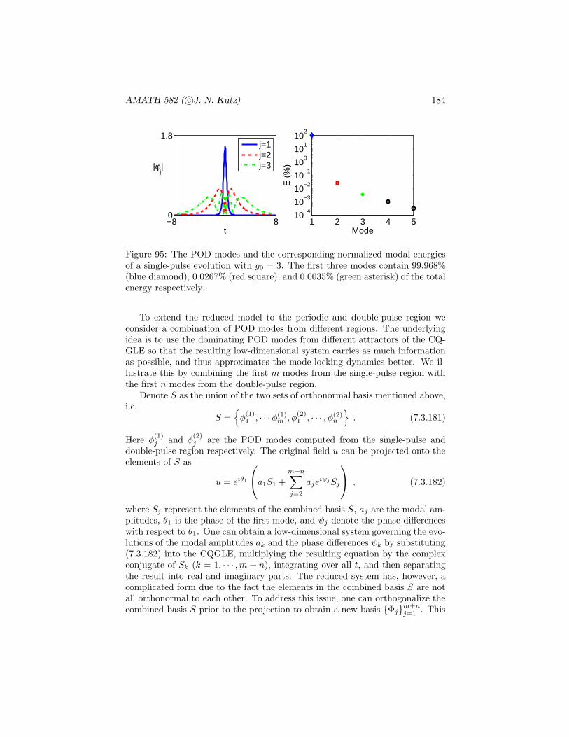
AMATH 582 ( c©J. N. Kutz) 184
1 2 3 4 510
−410
−310
−210
−110
010
110
2
E (
%)
Mode−8 80
1.8
|φj|
t
j=1j=2j=3
Figure 95: The POD modes and the corresponding normalized modal energiesof a single-pulse evolution with g0 = 3. The first three modes contain 99.968%(blue diamond), 0.0267% (red square), and 0.0035% (green asterisk) of the totalenergy respectively.
To extend the reduced model to the periodic and double-pulse region weconsider a combination of POD modes from different regions. The underlyingidea is to use the dominating POD modes from different attractors of the CQ-GLE so that the resulting low-dimensional system carries as much informationas possible, and thus approximates the mode-locking dynamics better. We il-lustrate this by combining the first m modes from the single-pulse region withthe first n modes from the double-pulse region.
Denote S as the union of the two sets of orthonormal basis mentioned above,i.e.
S ={φ
(1)1 , · · ·φ(1)
m , φ(2)1 , · · · , φ(2)
n
}. (7.3.181)
Here φ(1)j and φ
(2)j are the POD modes computed from the single-pulse and
double-pulse region respectively. The original field u can be projected onto theelements of S as
u = eiθ1
a1S1 +
m+n∑
j=2
ajeiψjSj
, (7.3.182)
where Sj represent the elements of the combined basis S, aj are the modal am-plitudes, θ1 is the phase of the first mode, and ψj denote the phase differenceswith respect to θ1. One can obtain a low-dimensional system governing the evo-lutions of the modal amplitudes ak and the phase differences ψk by substituting(7.3.182) into the CQGLE, multiplying the resulting equation by the complexconjugate of Sk (k = 1, · · · ,m + n), integrating over all t, and then separatingthe result into real and imaginary parts. The reduced system has, however, acomplicated form due to the fact the elements in the combined basis S are notall orthonormal to each other. To address this issue, one can orthogonalize thecombined basis S prior to the projection to obtain a new basis {Φj}m+n
j=1 . This

AMATH 582 ( c©J. N. Kutz) 185
1 2 3 4 510
−2
10−1
100
101
102
E (
%)
Mode−10 100
1.2
|φj(2)|
t
j=1j=2j=3
Figure 96: The POD modes and the corresponding normalized modal energiesof a double-pulse evolution of the CQGLE with g0 = 3.6 (cf. right column ofFig. 94). The first three modes contain 96.69% (blue diamond), 2.46% (redsquare), and 0.74% (green asterisk) of the total energy respectively.
can be achieved by the Gram-Schmidt algorithm given by
{Φ1 = S1 ,
Φj = χj/√〈χj , χj〉 , j = 2, · · · ,m+ n
(7.3.183)
where
χj = Sj −j−1∑
q=1
〈Sj ,Φq〉Φq , (7.3.184)
and the inner product is defined in standard way. The reduced model derivedfrom the new basis Φj has a simpler form than the one derived directly fromS, since it does not have terms that are due to non-orthogonality of the basisfunctions. This reduced model will be called the (m+n)-model, which indicatesthe number of modes taken from the single-pulse (m) and double-pulse region(n).
Before moving on to the investigation of the mode-locking dynamics gov-erned by the (m + n)-model, we first present the typical POD modes of adouble-pulse evolution of the CQGLE in Fig. 96. The dominating modes in
this case are φ(2)1 , φ
(2)2 , and φ
(2)3 , which takes up 99.9% of the total energy. As a
first approximation to the CQGLE dynamics, we consider the (1+3)-model since
the dominating mode in the single-pulse region is φ(1)1 (see Fig. 95). The or-
thonormal basis {Φj}4j=1 obtained using the Gram-Schmidt algorithm (7.3.183)
is shown in Fig. 97. By construction, the first mode Φ1 in the new basis is
identical to φ(1)1 . The second mode Φ2 contains a tall pulse which is identical
to the first mode at t = −6 and a small bump in the origin. In general thistall pulse can be located on either the left or the right of the origin, dependingon the data set U for which the POD modes are computed from. The other

AMATH 582 ( c©J. N. Kutz) 186
−10 0 100
1.6
|Φ1|
−10 0 100
1.6
|Φ2|
−15 0 150
0.5
|Φ3|
t−15 0 150
0.6
|Φ4|
t
Figure 97: Basis functions used in the (1+3)-model. These functions areobtained by applying the Gram-Schmidt algorithm (7.3.183) to the set S ={φ
(1)1 , φ
(2)1 , φ
(2)2 , φ
(2)3
}.
two modes have complicated temporal structures, and their oscillatory natureis mainly due to the orthogonalization. The (1+3)-model is derived from thesefour basis functions.
Classification of Solutions of the (1+3)-Model
The four-mode (1+3) model is 7-dimensional in the sense that the dynamicvariables are the four modal amplitudes a1, a2, a3, a4, and the three phasedifferences ψ2, ψ3, ψ4. To effectively characterize any periodic behavior in thesystem, it is customary to use the new set of variables
{x1 = a1 ,xj = aj cosψj , yj = aj sinψj
(7.3.185)
for j = 2, 3, 4 so that the formal projection of the field is given by
u = eiθ1
x1Φ1 +
∑
j≥2
(xj + iyj)Φj
. (7.3.186)
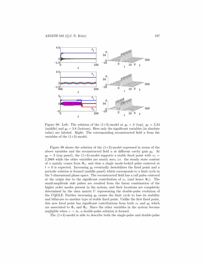
AMATH 582 ( c©J. N. Kutz) 187
0 100−1.5
0
4.5 x1
z
−10 0 10 0
5000
4
zt
|u|
495 500−1.5
0
4.5 x1
z
−10 0 10 0
5000
4
zt
|u|
0 200−5
0
5 x1
y2
z
−10 0 10 0
5000
4
zt
|u|
Figure 98: Left: The solution of the (1+3)-model at g0 = 3 (top), g0 = 3.24(middle) and g0 = 3.8 (bottom). Here only the significant variables (in absolutevalue) are labeled. Right: The corresponding reconstructed field u from thevariables of the (1+3)-model.
Figure 98 shows the solution of the (1+3)-model expressed in terms of theabove variables and the reconstructed field u at different cavity gain g0. Atg0 = 3 (top panel), the (1+3)-model supports a stable fixed point with x1 =2.2868 while the other variables are nearly zero, i.e. the steady state contentof u mainly comes from Φ1, and thus a single mode-locked pulse centered att = 0 is expected. Increasing g0 eventually destabilizes the fixed point and aperiodic solution is formed (middle panel) which corresponds to a limit cycle inthe 7-dimensional phase space. The reconstructed field has a tall pulse centeredat the origin due to the significant contribution of x1 (and hence Φ1). Thesmall-amplitude side pulses are resulted from the linear combination of thehigher order modes present in the system, and their locations are completelydetermined by the data matrix U representing the double-pulse evolution ofthe CQGLE. Further increasing g0 causes the limit cycle to lose its stabilityand bifurcate to another type of stable fixed point. Unlike the first fixed point,this new fixed point has significant contributions from both x1 and y2 whichare associated to Φ1 and Φ2. Since the other variables in the system becomenegligible when z → ∞, a double-pulse solution is formed.
The (1+3)-model is able to describe both the single-pulse and double-pulse

AMATH 582 ( c©J. N. Kutz) 188
0 1 2 3 4 5 6 72
4
6
8
10
12
g0
||u||2
StableUnstable
Figure 99: Bifurcation diagram of the total cavity energy of the reconstructedfield u as a function of g0. Here the bottom branch (blue) represents the single-pulse solution and the top branch (red) represents the double-pulse solution.The middle branch (green) denotes the extrema of the energy of the periodicsolution.
evolution of the CQGLE, which is a significant improvement compared to the 2-mode model considered in the previous section. The small-amplitude side pulsesin the reconstructed periodic solution do not appear at the expected locationspredicted by the CQGLE (see middle column of Fig. 94), since we are usingthe data with a particular gain (g0 = 3.6) to characterize the mode-lockingbehavior in the whole range of gain. Nevertheless, the two key features of theperiodic solution of the CQGLE are explicitly captured: (i) the existence of sidepulses, and (ii) the small-amplitude oscillations of the entire structure. Thesetwo features are not demonstrated by the reduced models considered before.The (1+3)-model also captures the amplification and suppression of the sidepulses in the formation of the double-pulse solution in the CQGLE. Since thePOD modes in the double-pulse region are computed from the numerical datawhere the left side pulse is chosen over the right side pulse (see Fig. 94), thesecond pulse in the reconstructed field always forms on the left. The case wherethe second pulse is formed on the right is not of particular interest since theunderlying dynamics is essentially the same.
AMATH 582 ( c©J. N. Kutz) 189
We construct a global bifurcation diagram in Fig. 99 to characterize the tran-sition between the single-pulse and double-pulse solution of the (1+3)-model.The diagram shows the total cavity energy of the reconstructed field u as a func-tion of the cavity gain g0, which is obtained using MATCONT [26]. In terms ofthe dynamic variables, the energy of the field is given by
‖u‖2 = x21 +
∑
j≥2
(x2j + y2
j
). (7.3.187)
In the diagram, the branch with the lowest energy corresponds to the singlemode-locked pulses of the (1+3)-model. With increasing g0, the reconstructedmode-locked pulse readjusts its amplitude and width accordingly to accommo-date the increase in the cavity energy. The branch of the single-pulse solutions isstable until g0 = 3.181 where a Hopf bifurcation occurs. The fluctuation in thecavity energy as a result of the periodic solution is small at first, but increasesgradually with g0. At g0 = 3.764 the periodic solution becomes unstable by afold bifurcation of the limit cycle. In this case a discrete jump is observed in thebifurcation diagram and a new branch of solutions is reached. This new branchrepresents the double-pulse solution of the system and has higher energy thanthe single-pulse branch and the periodic branch.
The bifurcation diagram also illustrates that in the region 1.681 ≤ g0 ≤ 3.181the single-pulse and the double-pulse solution are stable simultaneously. Thisbistability is not restricted to the (1+3)-model as it also happens in the CQGLEas well. Given a set of parameters, the final form of the solution is determinedby the basin of attraction of the single-pulse and double-pulse branches ratherthan the initial energy content. When the initial condition is selected suchthat it is “close” to the double-pulse branch (characterized by the Euclideandistance between them), the result of linear analysis holds and a double-pulsemode-locked state can be achieved. For random initial data that is far awayfrom both branches, the system tends to settle into the single-pulse branch asit is more energetically favorable.
Comparison of Different (m+n)-Models
To demonstrate that the (1+3)-model is the optimal (m+n)-model to char-acterize the transition from a single mode-locked pulse into two pulses thatoccurs in the CQGLE, we consider the (1+2)-model whose results are shownin the top row of Fig. 100. This model can be derived by setting the variablesx4 and y4 in the (1+3)-model to zero. At g0 = 3 a tall stable pulse in formedat t = −6 together with a small residual at the origin. The entire structurehas close resemblance to Φ2 from the Gram-Schmidt procedure. Except forthe location, the tall pulse agrees with the single-pulse solution of the CQGLEquantitatively. One can think of this as the result of the translational invari-ance of the CQGLE. In the full simulation of the CQGLE, the small residual

AMATH 582 ( c©J. N. Kutz) 190
Figure 100: Top: The reconstructed field of the (1+2)-model at g0 = 3 (left),g0 = 4.3 (middle), and g0 = 7 (right). Middle: The reconstructed field of the(1+4)-model at g0 = 3 (left), g0 = 3.4 (middle), and g0 = 3.8 (right). Bottom:The reconstructed field of the (2+3)-model at g0 = 3 (left), g0 = 3.4 (middle),and g0 = 3.7 (right).
is automatically removed by the intensity discriminating mechanism (saturableabsorption). When the structure loses its stability, a periodic solution is formedwhich persists even at unrealistically large values of cavity gain such as g0 = 7.
The middle row of the same figure shows the numerical simulations of the(1+4)-model, which is derived from the combination of the first POD modefrom the single-pulse region with the first four modes from the double-pulseregion. This model is able to reproduce all the key dynamics observed during themulti-pulsing phenomenon shown in Fig. 99. The difference between the (1+4)-model and the (1+3)-model is the locations at which the bifurcations occur. Inthe previous section we showed that the single-pulse solution described by the(1+3)-model loses stability at g0 = 3.181 (Hopf bifurcation), and the subsequentperiodic solution bifurcates into the double-pulse solution at g0 = 3.764. Forthe (1+4)-model these two bifurcations occur at g0 = 3.173 and g0 = 3.722

AMATH 582 ( c©J. N. Kutz) 191
respectively, which are closer to the values predicted using the CQGLE (g0 ≈3.15 and g0 ≈ 3.24). The (2+3)-model (bottom row of Fig. 100) produces similarresults as the (1+3)- and the (1+4)-model, with pulse transitions occurring at
g0 = 3.177 and 3.678. The comparison here shows that the third POD mode φ(2)3
from the double-pulse region is essential for getting the right pulse transition.Once this mode is included, further addition of the POD modes has only a minoreffect on the accuracy of the low-dimensional model.
8 Equation Free Modeling
Multiscale phenomena, and their associated complex systems, are an increas-ingly important class of problems that need to be addressed from a mathemat-ical point of view. As illustrated previously in the lecture on wavelets, somemathematical progress has been made in separating differing length scales bymore sophisticated (wavelet) transforms. Alternatively, one can think aboutthe difficulty in simulating both fine scale time and spatial features along sidecoarse time and spatial features. The recently developed equation-free model-ing concept allows for efficient simulations of complex, multiscale physics sys-tems without requiring the user to specify the system-level (coarse scale) equa-tions [27, 28, 29], thus providing a novel approach to computing such systems.
8.1 Multi-scale physics: an equation-free approach
It is often the case that in many systems of interest we know, or can derive,the microscopic description from some governing first principles. For instance,in atomic systems the Schrodinger equation can play the role of describing sin-gle atoms and their interactions. Similarly, F = ma is the starting point ofunderstanding many classical systems of interacting particles. Gas dynamicscan also be considered both at the microscopic level of atoms moving rapidlyand interacting with each other, or as a macroscopic collection of these atomswhich produce a temperature, pressure and volume. In this case, the gas can bemodeled with kinetic theory at the atomic level, or by something like the idealgas law at the macroscopically observable level.
The dichotomy in characteristic length scales between micro- and macro-physics is readily apparent in the above examples. Ultimately in constructingan appropriate mathematical description of the system, physically justifiableevolution equations, preferably derived from first principles, are critical for pre-dictive analysis of a given system. Often it is the case that the microscopicinteractions and dynamics are known and an attempt is made to systematicallyconstruct the macroscopic (observable) scale of interest from asymptotic or av-eraging arguments of the fine scale behavior. However, for sufficiently complexsystems, this may be an impossible task and instead, qualitative models areconstructed.
AMATH 582 ( c©J. N. Kutz) 192
As an example of such micro-to-macro-scale systems and dynamics, considerFigure 101 which exhibits a number of interesting patterns found in nature thatare clearly generated from a complex interaction at small scales in order to formcoherent patterns on the macroscopic scales of interest. These patterns rangefrom the development of clouds, which ultimately involves a large number ofinteracting water molecules, to sand patterns, which involves the interactions ofa tremendously large number of individual sand particles, to chemical reactions,which involves the interaction of two distinct species of chemical concentrates, tothe formation of patterns on sea shells and amoebas, which are functions of themicroscopic growth and chemicals released during the growth process. In manyof these cases, qualitative models can be constructed, such as the ubiquitousreaction-diffusion systems common in pattern forming systems. However, rarelyare these models connected back to the microscale which actually generated themacroscopic evolution equations.
To connect from the microscale to the macroscale, sophisticated mathemat-ical machinery is often brought to bear on the problem. This will be illustratedin the context of a many body quantum mechanical system where a mean-fieldapproach will be pursued. This will allow for a self-consistent, asymptoticallyjustified macroscopic evolution model. A similar approach can be taken in fluidmechanics: deriving the Navier-Stokes equations from the kinetic equations andinteraction at the molecular level of a fluid. Interestingly enough, the Navier-Stokes equations where known long before its justification from the atomic leveldescription, thus showing the power, importance, and necessity of macroscopicdescriptions.
Microscopic to macroscopic example: Bose-Einstine Condensation
To consider a specific model that allows the connection from the microscopicscale to the macroscopic scale, we examine mean-field theory of many-particlequantum mechanics with the particular application of BECs trapped in a stand-ing light wave [30]. The classical derivation given here is included to illustratehow the local model and its nonlocal perturbation are related. The inherentcomplexity of the dynamics of N pairwise interacting particles in quantum me-chanics often leads to the consideration of such simplified mean-field descrip-tions. These descriptions are a blend of symmetry restrictions on the particlewave function [31] and functional form assumptions on the interaction potential[31, 32, 33].
The dynamics of N identical pairwise interacting quantum particles is gov-erned by the time-dependent, N -body Schrodinger equation
i~∂Ψ
∂t=− ~2
2m∆NΨ+
N∑
i,j=1,i6=j
W (xi−xj)Ψ+N∑
i=1
V (xi)Ψ, (8.1.188)
where xi = (xi1, xi2, xi3), Ψ = Ψ(x1,x2,x3, ...,xN , t) is the wave function of

AMATH 582 ( c©J. N. Kutz) 193
Figure 101: Examples of ordered macroscopic phenomena generated from mi-croscale dynamics and interactions. In the first two examples, patterns in cloudformation are demonstrated. The second two figures are sand patterns thatappear due to interaction with tides (first picture) and in a desert. The spiraland target patterns in the next two figures are generated in chemical reactionsbetween two chemical species. Finally, the remaining three figures are from seashell patterns and a sea amoeba.
the N -particle system, ∆N =(∇N
)2=
∑Ni=1
(∂2xi1
+ ∂2xi2
+ ∂2xi3
)is the kinetic
energy or Laplacian operator for N -particles, W (xi − xj) is the symmetric in-teraction potential between the i-th and j-th particle, and V (xi) is an externalpotential acting on the i-th particle. Also, ~ is Planck’s constant divided by 2πand m is the mass of the particles under consideration.
One way to arrive at a mean-field description is by using the Lagrangian re-duction technique [34], which exploits the Hamiltonian structure of Eq. (8.1.188).The Lagrangian of Eq. (8.1.188) is given by [31]
L =
∫ ∞
−∞
{i~
2
(Ψ∂Ψ∗
∂t− Ψ∗∂Ψ
∂t
)+
~2
2m
∣∣∇NΨ∣∣2 +
N∑
i=1
N∑
j 6=i
W (xi − xj) + V (xi)
|Ψ|2
dx1 · · ·dxN . (8.1.189)
AMATH 582 ( c©J. N. Kutz) 194
The Hartree-Fock approximation (as used in [31]) for bosonic particles uses theseparated wave function ansatz
Ψ = ψ1(x1, t)ψ2(x2, t) · · ·ψN (xN , t) (8.1.190)
where each one-particle wave function ψ(xi) is assumed to be normalized sothat 〈ψ(xi)|ψ(xi)〉2 = 1. Since identical particles are being considered,
ψ1 = ψ2 = . . . = ψN = ψ, (8.1.191)
enforcing total symmetry of the wave function. Note that for the case of BECs,assumption (8.1.190) is approximate if the temperature is not identically zero.
Integrating Eq. (8.1.189) using (8.1.190) and (8.1.191) and taking the vari-ational derivative with respect to ψ(xi) results in the Euler-Lagrange equa-tion [34]
i~∂ψ(x, t)
∂t= − ~2
2m∆ψ(x, t)+V (x)ψ(x, t)+
(N−1)ψ(x, t)
∫ ∞
−∞
W (x−y)|ψ(y, t)|2dy. (8.1.192)
Here, x = xi, and ∆ is the one-particle Laplacian in three dimensions. TheEuler-Lagrange equation (8.1.192) is identical for all ψ(xi, t). Equation (8.1.192)describes the nonlinear, nonlocal, mean-field dynamics of the wave functionψ(x, t) under the standard assumptions (8.1.190) and (8.1.191) of Hartree-Focktheory [31]. The coefficient of ψ(x, t) in the last term in Eq. (8.1.192) representsthe effective potential acting on ψ(x, t) due to the presence of the other particles.
At this point, it is common to make an assumption on the functional formof the interaction potential W (x − y). This is done to render Eq. (8.1.192)analytically and numerically tractable. Although the qualitative features of thisfunctional form may be available, for instance from experiment, its quantitativedetails are rarely known. One convenient assumption in the case of short-rangepotential interactions is W (x − y) = κδ(x − y) where δ is the Dirac deltafunction. This leads to the Gross-Pitaevskii [32, 33] mean-field description:
i~∂ψ
∂t= − ~2
2m∆ψ + β|ψ|2ψ + V (x)ψ, (8.1.193)
where β = (N − 1)κ reflects whether the interaction is repulsive (β > 0)or attractive (β < 0). The above string of assumptions is difficult to phys-ically justify. Nevertheless, Lieb and Seiringer [35] show that Eq. (8.1.193)is the correct asymptotic description in the dilute-gas limit. In this limit,Eqs. (8.1.192) and (8.1.193) are asymptotically equivalent. Thus, althoughthe nonlocal Eq. (8.1.192) is in no way a more valid model than the localEq. (8.1.193), it can be interpreted as a perturbation to the local Eq. (8.1.193).

AMATH 582 ( c©J. N. Kutz) 195
Equation-free macroscopic modeling
In the case of the above mean-field model, or the Navier-Stokes, a systematicapproach can be taken to constructing the macroscopic governing equations.However, for sufficiently complex systems, this may not be possible, either be-cause there is no tractable analytic formalism, or the governing microscopicequations do not lend themselves to an asymptotic/averaging analysis. In thiscase, only the microscopic equations remain known and at the macroscopic levelone must resort to qualitative models which make no connection to the first prin-ciples of the system. Alternatively, the equation-free modeling technique allowsone to use the microscopic description to produce macroscopic observables alongwith their corresponding macroscopic time evolution without an explicit set ofmacroscopic equations. Thus we would like the following:
• System level (coarse or macroscopic) description of the system
• The macroscopic description should be “simple” (i.e. of significantly lowerdimension than the microscopic evolution)
• The macroscopic description should be practically predictive
• The macroscopic description should be computationally tractable, unlikethe complex microscopic system.
Ultimately, the problem formulation is a multi-scale (multi-resolution) typeproblem that has fine scale (microscopic) behavior which is only of marginalinterest in comparison to the coarse (macroscopic) behavior.
Mathematically, the problem formulation results in an attempt to constructthe macroscopic dynamical evolution, for instance, as system of differential equa-tions:
dx
dt= f(x) (8.1.194)
where the behavior is determined by f(x). Such a system can be easily solvedcomputationally by using a standard time-stepping algorithm. Specifically, con-sider the Euler time stepping algorithm which simply makes use of a slope for-mula and the definition of derivative:
xn+1 = xn + ∆tf(xn) . (8.1.195)
Provided we know f(x), the solution can easily be advanced in time by timesteps ∆t. But here is the point: we don’t know f(x)! Regardless, the Eulermethod essentially provides a template, or protocol, for specifying where toperform function evaluations. A couple key observations should be stated atthis point:
• An explicit representation of function f(x) is not needed, rather only thediscrete values at f(xn) are necessary.

AMATH 582 ( c©J. N. Kutz) 196
• The function f(xn) could be evaluated through a variety of techniquesincluding a table lookup, simulation or from experiment itself.
• The sequence xn is not known a priori, but must be determined as partof the computational task.
• The protocol is determined from a underlying algorithm associated withthe macroscopic evolution equations.
Thus our objective is in the construction of f(xn) by any means at discretepoints. Indeed, the above arguments lead us to consider the following algorithm(to be explored in detail in the next section) for evolving on the macroscopicscale.
1. Estimate the initial state of the system x(t = 0).
2. Simulate the microscale physics for a short time in order to estimate dx/dt.
3. Take a “big” mesoscale step into the future, i.e. a time-step much largerthan the microscale system allows, but on the time-step scale of themacrosystem.
4. repeat
This algorithm is the shell of what the equation-free approach does. Indeed, thepurpose is simply to use the microscale to estimate, not specify, the macroscopicevolution f(x). Key to this algorithm will be our ability to go between themicro- and macro-scales. The process of going from micro to macro is known asrestriction whereas the macro to macro is termed lifting. Both of these conceptsand operations will be considered in detail in the next section. Figure 102demonstrates graphically the process undertaken in the above algorithm. In thetop plot, the standard Euler algorithm is considered where the function f(x) isknown. The bottom plot shows the equation-free process by which a burst ofmicroscale simulation generates a numerical approximation to f(x) giving thenecessary projection to the future.
8.2 Lifting and restricting in equation-free computing
We are interested in the macroscopic behavior of large complex systems. Thiswill be the scale of interest in our given application. Two assumptions will bemade: only the microscopic (fine scale) equations of motion are available, andthe macroscopic (coarse scale) equations are unknown. The microscopic vari-ables are often not directly represented in the macroscopic formulation. Forinstance, for a gas simulation, the individual gas particle velocities and distri-butions are of critical importance in the computation of the fine scale equationsof motion and state. On the macroscopic level, however, the interest is the gas
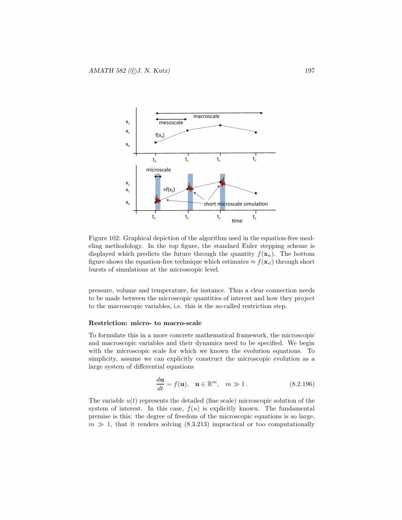
AMATH 582 ( c©J. N. Kutz) 197
!"# !$#!%# !&#
!$#!%# !&#!"#
'"#
'%#
'$#
'"#
'%#
'$#
()'"*##
+()'"*##
,-.#
/012!#-3421/456.#/3-765,18#
-5421/456.#
-./1/456.#
-3421/456.#
Figure 102: Graphical depiction of the algorithm used in the equation-free mod-eling methodology. In the top figure, the standard Euler stepping scheme isdisplayed which predicts the future through the quantity f(xn). The bottomfigure shows the equation-free technique which estimates ≈ f(xn) through shortbursts of simulations at the microscopic level.
pressure, volume and temperature, for instance. Thus a clear connection needsto be made between the microscopic quantities of interest and how they projectto the macroscopic variables, i.e. this is the so-called restriction step.
Restriction: micro- to macro-scale
To formulate this in a more concrete mathematical framework, the microscopicand macroscopic variables and their dynamics need to be specified. We beginwith the microscopic scale for which we known the evolution equations. Tosimplicity, assume we can explicitly construct the microscopic evolution as alarge system of differential equations
du
dt= f(u), u ∈ Rm, m≫ 1 . (8.2.196)
The variable u(t) represents the detailed (fine scale) microscopic solution of thesystem of interest. In this case, f(u) is explicitly known. The fundamentalpremise is this: the degree of freedom of the microscopic equations is so large,m ≫ 1, that it renders solving (8.3.213) impractical or too computationally
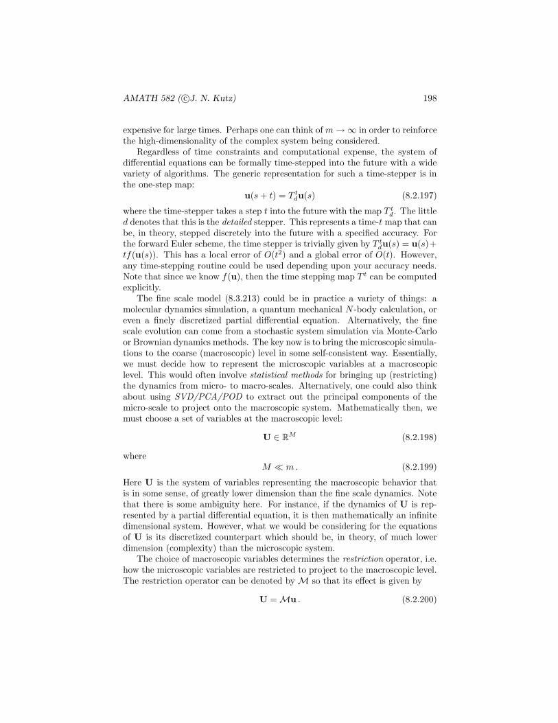
AMATH 582 ( c©J. N. Kutz) 198
expensive for large times. Perhaps one can think of m→ ∞ in order to reinforcethe high-dimensionality of the complex system being considered.
Regardless of time constraints and computational expense, the system ofdifferential equations can be formally time-stepped into the future with a widevariety of algorithms. The generic representation for such a time-stepper is inthe one-step map:
u(s+ t) = T tdu(s) (8.2.197)
where the time-stepper takes a step t into the future with the map T td. The littled denotes that this is the detailed stepper. This represents a time-t map that canbe, in theory, stepped discretely into the future with a specified accuracy. Forthe forward Euler scheme, the time stepper is trivially given by T tdu(s) = u(s)+tf(u(s)). This has a local error of O(t2) and a global error of O(t). However,any time-stepping routine could be used depending upon your accuracy needs.Note that since we know f(u), then the time stepping map T t can be computedexplicitly.
The fine scale model (8.3.213) could be in practice a variety of things: amolecular dynamics simulation, a quantum mechanical N -body calculation, oreven a finely discretized partial differential equation. Alternatively, the finescale evolution can come from a stochastic system simulation via Monte-Carloor Brownian dynamics methods. The key now is to bring the microscopic simula-tions to the coarse (macroscopic) level in some self-consistent way. Essentially,we must decide how to represent the microscopic variables at a macroscopiclevel. This would often involve statistical methods for bringing up (restricting)the dynamics from micro- to macro-scales. Alternatively, one could also thinkabout using SVD/PCA/POD to extract out the principal components of themicro-scale to project onto the macroscopic system. Mathematically then, wemust choose a set of variables at the macroscopic level:
U ∈ RM (8.2.198)
whereM ≪ m. (8.2.199)
Here U is the system of variables representing the macroscopic behavior thatis in some sense, of greatly lower dimension than the fine scale dynamics. Notethat there is some ambiguity here. For instance, if the dynamics of U is rep-resented by a partial differential equation, it is then mathematically an infinitedimensional system. However, what we would be considering for the equationsof U is its discretized counterpart which should be, in theory, of much lowerdimension (complexity) than the microscopic system.
The choice of macroscopic variables determines the restriction operator, i.e.how the microscopic variables are restricted to project to the macroscopic level.The restriction operator can be denoted by M so that its effect is given by
U = Mu . (8.2.200)

AMATH 582 ( c©J. N. Kutz) 199
It is this step that either averages over the fine scales (in both space and time)or applies some low-rank approximation which may come from, for instance, theSVD/PCA/POD formalism. Other methods include the maximum likelihoodinference model and the cumulative probability distribution for generating therestriction operator.
Lifting: macro- to micro-scale
If the microscopic system can be successfully modeled at the macroscopic scaleby the set of variables U, the remaining statistical quantities at the micro-scale should be well approximated by functionals of the selected ones used forthe restriction operation. To illustrate this, consider the transformation of themicroscopic dynamics to a new set of variables
u 7→ v (8.2.201)
which gives a system of differential equations
dv
dt= g(v1,v2) (8.2.202)
where v = (v1,v2) is partitioned into M and m −M components. Further,the compatible partition g is (g1, g2/ǫ) with ǫ ≪ 1. This gives the system ofequations
dv1
dt= g1(v1,v2) ∈ RM (8.2.203a)
dv2
dt=
1
ǫg2(v1,v2) ∈ Rm−M . (8.2.203b)
This formalism gives a multi-scale or multi-resolution mathematical architec-ture that can be used to construct a self-consistent fast-/slow-scale analysis.Specifically, the variable v2 represents the fast scale dynamics of the micro-scale. Since it is a fast scale, it should reach its steady-state behavior ratherquickly (or some slow manifold). Thus v2 closes to v1 so that v2 = r(v1) whereg2(v1, r(v1)) = 0. The variable v1 can then be identified with the macroscopicvariable U so that
dU
dt=dv1
dt= g1(v1, r(v1)) = F (U) . (8.2.204)
The only way for this to make sense is for us to be able to systematicallyconstruct the unknown functions g, r and F , i.e. they are not known in closedform, but rather constructed computationally from the fine scale simulationsand the restriction process. This is what gives it the name equation-free sincethe macroscopic governing equations F (U) are not known.

AMATH 582 ( c©J. N. Kutz) 200
If the construction of F (U) can be performed, then Eq. (8.2.204) can bestepped forward in time with
U(t + τ) = T τc U(t) (8.2.205)
where the time-stepper takes a step τ into the future with the map T τc . Thelittle c denotes that this is the coarse stepper. As before, this represents a time-τ map that can be, in theory, stepped discretely into the future with a specifiedaccuracy. The parameter τ > 0 is the time horizon of the coarse time stepper.The length of time τ appropriate for this problem is such that it renders thecomputation of the complex system tractable. Specifically, it must be chosen tobe small enough on the macro-scale so that good accuracy can be achieved at thecoarse scale, yet it must be chosen big enough so that micro-scale simulationscan be short enough to be tractable.
The coarse time-stepper relies on a variety of factors, including the ability ofthe algorithm to project back the macroscopic details to the microscopic system.This project from coarse to fine detail is called the lifting operation and it isdenoted by µ. The lifting operation is philosophically equivalent to the inverseof the restriction operation M. Thus for consistency:
Mµ = I (8.2.206)
where I is the identify operator. Thus the combination of lifting and restrictionallows flexibility to move in and out of the micro- and macro-scales.
Equation-free algorithm
With the mathematical concept of lifting and restriction in place, an algorithmcan be presented for performing complex, high-dimensional, multi-scale model-ing. The following is the outline of the algorithm that would be used assuminga macroscopic condition U(t) is specified at some moment in time.
1. Lift: Transform the initial data on the coarse scale to one (or more) fine,consistent microscopic realizations u(s, t), i.e. use the lifting operator toproduce u(0, t) = µU.
2. Evolve: The microscopic simulator can then be applied to advance thefine scale initial data a short, macroscopic time τ . Thus the followingevolution in time is constructed: u(τ, t) = T τd u(0, t).
3. Restrict: Obtain the restriction of u so that the coarse time-stepperevolution can be constructed from T τc U(t) = Mu(τ, t).
The algorithm is then repeated to continue advancing the solution into thefuture. Effectively, you are replacing the full evolution by a multiscale approachwhere short bursts of the fine scale simulations are used to generate large timesteps at the coarse level.

AMATH 582 ( c©J. N. Kutz) 201
The above algorithm shows that the coarse stepper is thus defined by
T τc = MT τd µ . (8.2.207)
which is a combination of repeated lifting, fine-scale evolution and restriction.No equations are ever specified at the large (coarse or macroscopic) scale, nordo they need to be specified. It is equation-free.
A few things are worth noting in the above formulation. The first is thatthe choice of lifting µ determines the initial condition for v2 at time t inEq. (8.2.203b). For a simulation time s ≫ ǫ, and with the assumption thatv2 approximately reduces to a function of v1 given by g2 ≈ 0 (independentof the initial state), the equation quickly approaches the slow-manifold for anylifting operator µ. Thus after some initial transient, the dynamics is well ap-proximated by Eq. (8.2.204) and U(t + s) ≈ Mu(s, t). More importantly, thederivates of Mu(s, t) will also be a good approximation to the derivatives ofU(t + s) after the transient time. We will thus use the derivatives of Mu(s, t)to approximate the derivatives of U(t + s) and thereby create the coarse timestepper T τc .
Coarse projection integration
The final step in the equation-free algorithm is to make use the short time,fine scale simulations to take large time steps on the macroscopic time scale.Thus a high-degree of computational can be readily achieved. Mathematicallyspeaking, we would like to simulate the macroscopic equation (8.2.204) for timest≫ τ . Coarse projection integration will allow us to take the short time coarsetime-stepper and perform long time (system level) tasks.
To understand the coarse projection integration, consider the following twotime-scales
∆t large time step (slow coarse dynamics)
δt small time step (fast, transient, micro-scale dynamics) .
Further let the following scaling hold
δt ≤ τ ≪ ∆t . (8.2.208)
The step δt is often thought of as the numerical time step of the microscopicevolution (8.3.213). By setting tk = kδt and defining U(t) as UN ≈ U(N∆t),the we can consider the action of the microscopic time-stepper
uk,N = T tkd u0,N (8.2.209)
where u0,N = µUN . As long as the number of small time steps, k, remainsrelatively small so that tk = kδt = O(τ), then this step can be afforded compu-tationally.
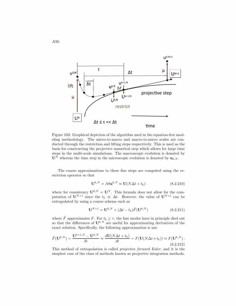
AMATH 582 ( c©J. N. Kutz) 202
!"#$
%&$
'()&$
'*)&$'*+,)&$
%*+,)&$
%*)&$
%&+,$
'()&+,$
-.$
/.$
0#1.023.$
425$
6078#3!9#$1.#6$:$
:$
!"
;$
/.$<$;$==$/.$
Figure 103: Graphical depiction of the algorithm used in the equation-free mod-eling methodology. The micro-to-macro and macro-to-micro scales are con-ducted through the restriction and lifting steps respectively. This is used as thebasis for constructing the projective numerical step which allows for large timesteps in the multi-scale simulations. The macroscopic evolution is donated byUN whereas the time step in the microscopic evolution is denoted by uk,N .
The coarse approximations to these fine steps are computed using the re-striction operator so that
Uk,N = Muk,N ≈ U(N∆t+ tk) (8.2.210)
where for consistency U0,N = UN . This formula does not allow for the com-putation of UN+1 since the tk ≪ ∆t. However, the value of UN+1 can beextrapolated by using a coarse scheme such as
UN+1 = Uk,N + (∆t− tk)F (Uk,N ) (8.2.211)
where F approximates F . For tk ≥ τ , the fast modes have in principle died outso that the differences of Uk,N are useful for approximating derivatives of theexact solution. Specifically, the following approximation is use:
F (Uk,N ) =Uk+1,N − Uk,N
δt≈ dU(N∆t+ tk)
dt= F (U(N∆t+ tk)) ≈ F (Uk,N ) .
(8.2.212)This method of extrapolation is called projective forward Euler, and it is thesimplest case of the class of methods known as projective integration methods.
AMATH 582 ( c©J. N. Kutz) 203
This is the explicit outer integrator that is built around the inner integratorassociated with the fine scale simulations.
Thus the coarse scale time evolution as modeled by (8.2.204) is performed byapproximations of F achieved by the fine scale simulations. The entire processis represented in Fig. 103 where the interaction of the fine scale, course scale,projective stepping along with the lifting/restriction operations are identified.It is quite a remarkable process that potentially can allow for a highly im-proved, and computationally tractable, methodologies for handling multi-scaleproblems. Part of the connection here to data analysis is in the projection andlifting operators: many of the techniques we have considered could be used toperform these critical operations.
8.3 Equation-free space-time dynamics
The discussion in the previous section highlighted the ability of the equation-free algorithm to advance in time a numerical solution on a coarse scale, viaan Euler projective time-step, given simulations on the microscopic time scale.In this section, we extend this idea to include both time- and space-evolutiondynamics. Specifically, we consider the case when the microscopic equations ofmotion both occur on fast scales in relation to the macroscopic observations ofinterest.
Mathematically, the analytic framework considered on the microscale is nowmodified to
du
dt= f(u), u ∈ Rm, m≫ 1 + boundary conditions. (8.3.213)
where the variable u(t) once again represents the detailed (fine scale) microscopicsolution of the system of interest. In this case, f(u) is explicitly known to be afunction of both space and time. As before, the fundamental premise is this: thedegree of freedom of the microscopic equations is so large,m≫ 1, that it renderssolving (8.3.213) impractical or too computationally expensive for large times.Perhaps one can think of m → ∞ in order to reinforce the high-dimensionalityof the complex system being considered.
At the course (macroscopic) level, the equations of motion are now governedby a partial-differential equation of time and space so that
∂U
∂t= L
(t,x,U,
∂U
∂x,∂2U
∂x2, · · · , ∂
pU
∂xp
)(8.3.214)
where U(t,x) is the macroscopic variable of interest and L is a general integro-differential operator of degree p in space x. The operator L is in general, non-linear. Further, it is unknown given the premise that it is too complicated toachieve an averaging or asymptotic scheme capable of deriving it from the mi-croscopic description. The goal once again is then to approximate L throughmicroscopic simulations versus actually explicitly constructing it.
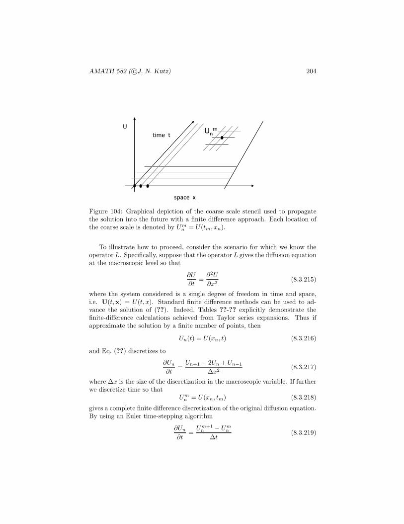
AMATH 582 ( c©J. N. Kutz) 204
!"
#$%&'""("
)*'""+"!,
*"
Figure 104: Graphical depiction of the coarse scale stencil used to propagatethe solution into the future with a finite difference approach. Each location ofthe coarse scale is denoted by Umn = U(tm, xn).
To illustrate how to proceed, consider the scenario for which we know theoperator L. Specifically, suppose that the operator L gives the diffusion equationat the macroscopic level so that
∂U
∂t=∂2U
∂x2(8.3.215)
where the system considered is a single degree of freedom in time and space,i.e. U(t,x) = U(t, x). Standard finite difference methods can be used to ad-vance the solution of (??). Indeed, Tables ??-?? explicitly demonstrate thefinite-difference calculations achieved from Taylor series expansions. Thus ifapproximate the solution by a finite number of points, then
Un(t) = U(xn, t) (8.3.216)
and Eq. (??) discretizes to
∂Un∂t
=Un+1 − 2Un + Un−1
∆x2(8.3.217)
where ∆x is the size of the discretization in the macroscopic variable. If furtherwe discretize time so that
Umn = U(xn, tm) (8.3.218)
gives a complete finite difference discretization of the original diffusion equation.By using an Euler time-stepping algorithm
∂Un∂t
=Um+1n − Umn
∆t(8.3.219)
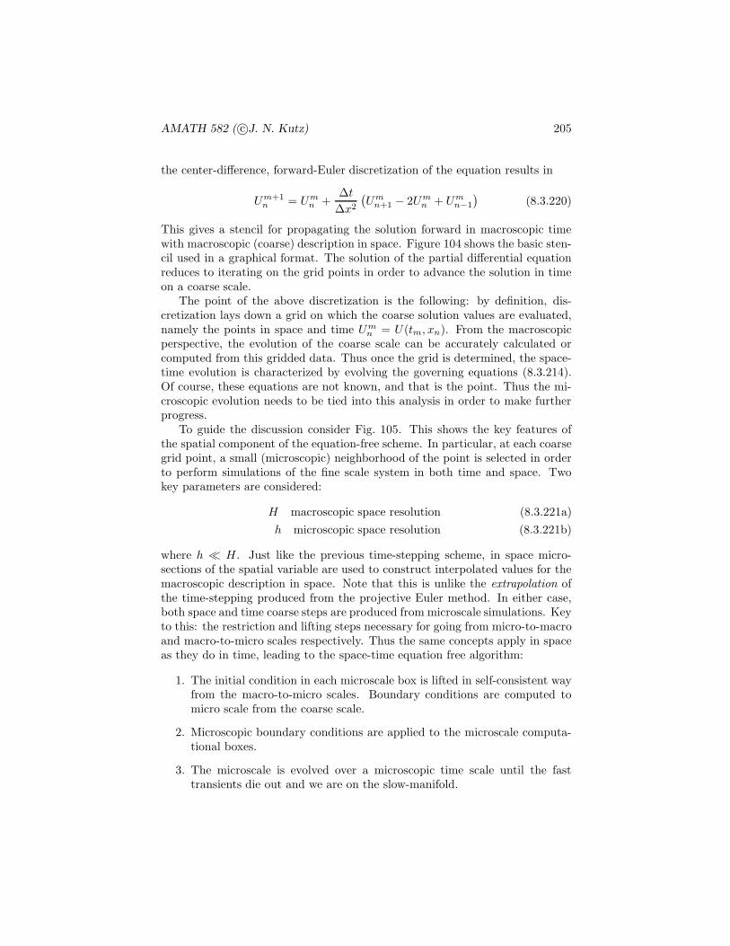
AMATH 582 ( c©J. N. Kutz) 205
the center-difference, forward-Euler discretization of the equation results in
Um+1n = Umn +
∆t
∆x2
(Umn+1 − 2Umn + Umn−1
)(8.3.220)
This gives a stencil for propagating the solution forward in macroscopic timewith macroscopic (coarse) description in space. Figure 104 shows the basic sten-cil used in a graphical format. The solution of the partial differential equationreduces to iterating on the grid points in order to advance the solution in timeon a coarse scale.
The point of the above discretization is the following: by definition, dis-cretization lays down a grid on which the coarse solution values are evaluated,namely the points in space and time Umn = U(tm, xn). From the macroscopicperspective, the evolution of the coarse scale can be accurately calculated orcomputed from this gridded data. Thus once the grid is determined, the space-time evolution is characterized by evolving the governing equations (8.3.214).Of course, these equations are not known, and that is the point. Thus the mi-croscopic evolution needs to be tied into this analysis in order to make furtherprogress.
To guide the discussion consider Fig. 105. This shows the key features ofthe spatial component of the equation-free scheme. In particular, at each coarsegrid point, a small (microscopic) neighborhood of the point is selected in orderto perform simulations of the fine scale system in both time and space. Twokey parameters are considered:
H macroscopic space resolution (8.3.221a)
h microscopic space resolution (8.3.221b)
where h ≪ H . Just like the previous time-stepping scheme, in space micro-sections of the spatial variable are used to construct interpolated values for themacroscopic description in space. Note that this is unlike the extrapolation ofthe time-stepping produced from the projective Euler method. In either case,both space and time coarse steps are produced from microscale simulations. Keyto this: the restriction and lifting steps necessary for going from micro-to-macroand macro-to-micro scales respectively. Thus the same concepts apply in spaceas they do in time, leading to the space-time equation free algorithm:
1. The initial condition in each microscale box is lifted in self-consistent wayfrom the macro-to-micro scales. Boundary conditions are computed tomicro scale from the coarse scale.
2. Microscopic boundary conditions are applied to the microscale computa-tional boxes.
3. The microscale is evolved over a microscopic time scale until the fasttransients die out and we are on the slow-manifold.
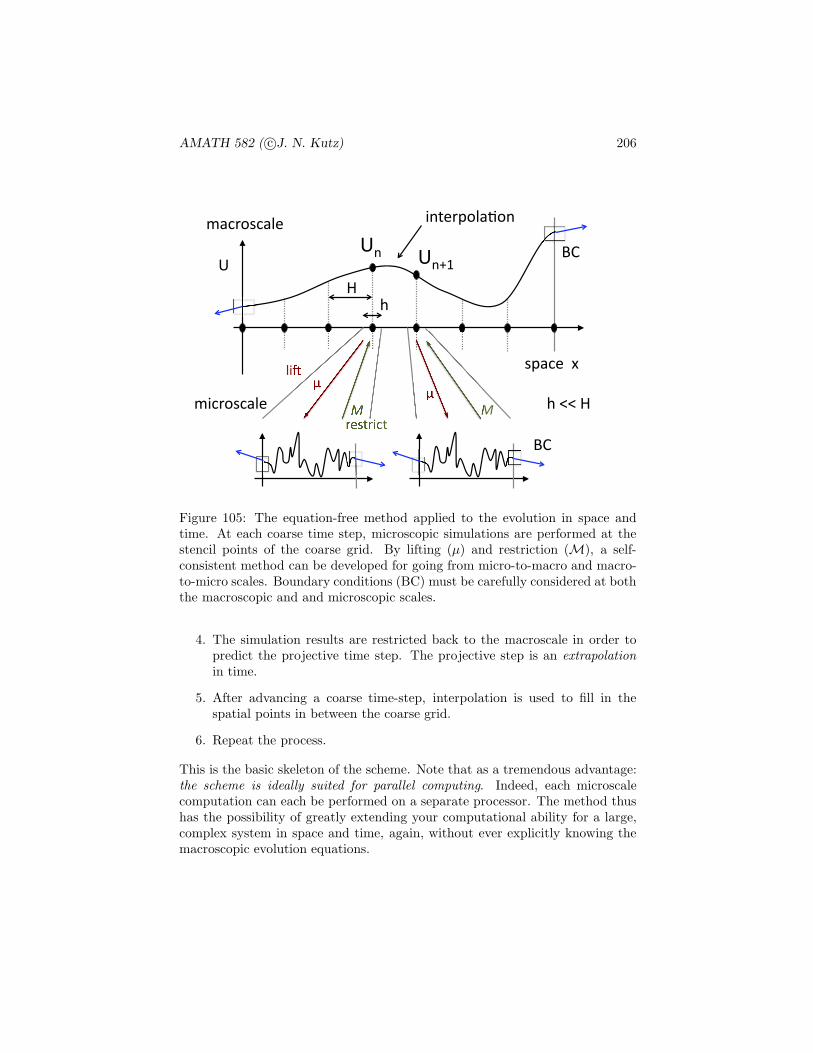
AMATH 582 ( c©J. N. Kutz) 206
!"
#$%&'""("
!)" !)*+"
,)-'.$/0%1/)"2%&./#&%0'"
2,&./#&%0'"
.'#-.,&-"
0,3"4"
!"
4"
!"
56"
56"
7"8"
8"99"7"
Figure 105: The equation-free method applied to the evolution in space andtime. At each coarse time step, microscopic simulations are performed at thestencil points of the coarse grid. By lifting (µ) and restriction (M), a self-consistent method can be developed for going from micro-to-macro and macro-to-micro scales. Boundary conditions (BC) must be carefully considered at boththe macroscopic and and microscopic scales.
4. The simulation results are restricted back to the macroscale in order topredict the projective time step. The projective step is an extrapolationin time.
5. After advancing a coarse time-step, interpolation is used to fill in thespatial points in between the coarse grid.
6. Repeat the process.
This is the basic skeleton of the scheme. Note that as a tremendous advantage:the scheme is ideally suited for parallel computing. Indeed, each microscalecomputation can each be performed on a separate processor. The method thushas the possibility of greatly extending your computational ability for a large,complex system in space and time, again, without ever explicitly knowing themacroscopic evolution equations.
AMATH 582 ( c©J. N. Kutz) 207
References
[1] M. R. Spiegel, Probability and Statistics, (Schaum’s Outline Series,McGraw-Hill, 1975)
[2] S. Ross, Introduction to Probability Models, 4th Ed. (Academic Press, 1989).
[3] W. H. Press, S. A. Teukolsky, W. T. Vetterling, B. P. Flannery, NumericalRecipes, 2nd Ed. (Cambridge, 1992).
[4] L. Debonath, Wavelet Transforms and Their Applications (Birkhauser,2002).
[5] A. Haar, “Zur Theorie der orthogonalen funktionen-systeme,” Math. Ann.69, 331-371 (1910).
[6] T. F. Chan and J. Shen, Image processing and analysis, (SIAM, Philadel-phia, 2005).
[7] L. N. Trefethen and D. Bau, Numerical Linear Algebra, (SIAM, Philadel-phia, 1997).
[8] J. Shlens, “A tutorial on principal component analysis,” (available on theweb).
[9] P. Holmes, J. L. Lumley, and G. Berkooz, Turbulence, Coherent Structures,Dynamical Systems, and Symmetry, (Cambridge, 1996).
[10] J. P. Cusumano, M. T. Sharkady, and B. W. Kimble, “Dynamics of aflexible beam impact oscillator,” Philos. Trans. R. Soc. London347, 421-438 (1994).
[11] B. F. Feeny and R. Kappagantu, “On the physical interpretation of properorthogonal modes in vibrations,” J. Sound Vibr. 211, 607-616 (1998).
[12] T. Kubow, M. Garcia, W. Schwind, R. Full, R., and D. E. Koditschek, “Aprincipal components analysis of cockroach steady state leg motion,” (inpreparation)
[13] R. Ruotolo and C. Surace, “Damage assessment of multiple cracked beams:numerical results and experimental validation.” J. Sound Vibr. 206, 567588(1997).
[14] K. L. Briggman, H. D. I. Abarbanel, W. B. Kristan Jr. “Optical Imaging ofNeuronal Populations During Decision-Making,” Science 307, 896 (2005).
[15] A. Chatterjee, “An introduction to the proper orthogonal decomposition,”Current Science 78, 808-817 (2000).
AMATH 582 ( c©J. N. Kutz) 208
[16] J. Tenenbaum, V. de Silva and J. C. Langford, “A Global Geometric Frame-work for Nonlinear Dimensionality Reduction,” Science 290, 2319-2323
[17] S. Roweis and L. K. Saul, “Linear EmbeddingNonlinear DimensionalityReduction by Locally Linear Embedding,” Science 290, 2323-2326 (2000).
[18] K. Q. Weinberger and L. K. Saul, “Unsupervised Learning of Image Mani-folds by Semidenite Programming,” Int. J. Comp. Vision 70, 77-90 (2006).
[19] A. Hyvarinen and E. Oja, “Independent Component Analysis: Algorithmsand Applications,” (available on the web)
[20] H. Farid and E. H. Adelson, “Separating reflections from images by useof independent component analysis,” J. Opt. Soc. Am. A 16, 2136-2145(1999).
[21] R. A. Fisher, “The Use of Multiple Measurements in Taxonomic Problems,”Annals of Eugenics 7, 179188 (1936).
[22] E. Ding, E. Shlizerman and J. N. Kutz, “Modeling multipulsing transitionin ring cavity lasers with proper orthogonal decomposition,” Phys. Rev. A82, 023823 (2010).
[23] H. A. Haus, “Mode-locking of lasers,” IEEE J. Sel. Top. Quant. Elec. 6,1173 (2000).
[24] J. N. Kutz, “Mode-locked soliton lasers,” SIAM Rev. 48, 629 (2006).
[25] S. Namiki, E. P. Ippen, H. A. Haus, and C. X. Yu, ”Energy rate equationsfor mode-locked lasers,” J. Opt. Soc. Am. B 14, 2099 (1997).
[26] A. Dhooge, W. Govaerts, and Yu. A. Kuznetsov, ACM Transactions onMathematical Software 29, 141 (2003).
[27] I. G. Kevrekidis, C. W. Gear and G. Hummer, “Equation Free: TheComputer-Aided Analysis of Complex Multiscale Systems,” Am. Inst.Chem. Eng. 50, 1346-1355 (2004).
[28] B. A. Cipra, “Equation-Free Computing Gets Something from (Almost)Nothing,” SIAM News 38, (2005).
[29] I. G. Kevrekidis, C. W. Gear, J. M. Hyman, P. G. Kevrekidis, O. Run-borg, C. Theodoropoulos, “Equation-free, course-grained multiscale com-putation: enabling microscopic simulators to perform system-level analy-sis,” Comm. Math. Sci. 1, 715-762 (2003).
[30] B. Deconinck and J. N. Kutz, “Singular instability of exact stationary so-lutions of the nonlocal Gross-Pitaevskii equation,” Physical Letters A 319,97-103 (2003).

AMATH 582 ( c©J. N. Kutz) 209
[31] G. Baym, Lectures in Quantum Mechanics, Addison-Wesley (RedwoodCity, CA, 1990).
[32] E. P. Gross, Nuovo Cimento 20, 454 (1961).
[33] L. P. Pitaevskii, Sov. Phys. JETP 13, 451 (1961).
[34] G. B. Whitham, Linear and Nonlinear Waves, Wiley (New York, NY,1974).
[35] E. H. Lieb and R. Seiringer, Phys. Rev. Lett. 88, 170409 (2002).


