aMassimo Bertolini , Marcello Braglia , Giovanni … · Extending value stream mapping: the...

This article was downloaded by: [Università degli Studi di Parma], [Dr Massimo Bertolini]On: 18 September 2013, At: 00:00Publisher: Taylor & FrancisInforma Ltd Registered in England and Wales Registered Number: 1072954 Registered office: Mortimer House,37-41 Mortimer Street, London W1T 3JH, UK

International Journal of Production ResearchPublication details, including instructions for authors and subscription information:http://www.tandfonline.com/loi/tprs20

Extending value stream mapping: the synchro-MRPcaseMassimo Bertolini a , Marcello Braglia b , Giovanni Romagnoli a & Francesco Zammori aa Dipartimento di Ingegneria Industriale , Università degli Studi di Parma , Parma , Italyb Dipartimento di Ingegneria Meccanica , Nucleare e della Produzione , Pisa , ItalyPublished online: 09 Jun 2013.

To cite this article: Massimo Bertolini , Marcello Braglia , Giovanni Romagnoli & Francesco Zammori (2013) Extendingvalue stream mapping: the synchro-MRP case, International Journal of Production Research, 51:18, 5499-5519, DOI:10.1080/00207543.2013.784415

To link to this article: http://dx.doi.org/10.1080/00207543.2013.784415

PLEASE SCROLL DOWN FOR ARTICLE

Taylor & Francis makes every effort to ensure the accuracy of all the information (the “Content”) containedin the publications on our platform. However, Taylor & Francis, our agents, and our licensors make norepresentations or warranties whatsoever as to the accuracy, completeness, or suitability for any purpose of theContent. Any opinions and views expressed in this publication are the opinions and views of the authors, andare not the views of or endorsed by Taylor & Francis. The accuracy of the Content should not be relied upon andshould be independently verified with primary sources of information. Taylor and Francis shall not be liable forany losses, actions, claims, proceedings, demands, costs, expenses, damages, and other liabilities whatsoeveror howsoever caused arising directly or indirectly in connection with, in relation to or arising out of the use ofthe Content.

This article may be used for research, teaching, and private study purposes. Any substantial or systematicreproduction, redistribution, reselling, loan, sub-licensing, systematic supply, or distribution in anyform to anyone is expressly forbidden. Terms & Conditions of access and use can be found at http://www.tandfonline.com/page/terms-and-conditions

http://www.tandfonline.com/loi/tprs20

http://www.tandfonline.com/action/showCitFormats?doi=10.1080/00207543.2013.784415

http://dx.doi.org/10.1080/00207543.2013.784415

http://www.tandfonline.com/page/terms-and-conditions

http://www.tandfonline.com/page/terms-and-conditions

Extending value stream mapping: the synchro-MRP case

Massimo Bertolinia*, Marcello Bragliab, Giovanni Romagnolia and Francesco Zammoria

aDipartimento di Ingegneria Industriale, Università degli Studi di Parma, Parma, Italy; bDipartimento di Ingegneria Meccanica,Nucleare e della Produzione, Pisa, Italy

(Received 9 May 2012; final version received 23 February 2013)

Nowadays, value stream mapping (VSM) is recognised as the main tool for implementing lean manufacturing.Unfortunately, it always leads to pure pull systems and discourages the adoption of hybrid push/pull ones, although theirsuperiority has been proven in several industrial settings. Due to these issues, this paper presents an enhancement of thestandard VSM, which supports the user in designing the future state map of a synchro-MRP system. This new toolincludes new mapping icons, simple mathematical formulas and operating guidelines that make it possible to assess thebenefits of a synchro-MRP system, with respect to the usual kanban or CONWIP ones. In order to demonstrate thequality and the practical utility of the proposed approach, an industrial application of relevance is finally presented.

Keywords: value stream mapping; lean manufacturing; synchro-MRP; hybrid push/pull systems

1. Introduction

During the last decades, lean thinking has emerged as one of the most influential paradigms, both in manufacturing andmanagement (Hines, Holweg, and Rich 2004). From a holistic and philosophical perspective, lean can be seen as a setof general principles and ultimate ends guiding strategic decisions. At a more practical level, it can be described as acombination of operating tools and shop floor techniques, aiming to boost manufacturing performances through work inprocess (WIP) reduction and flow time stabilisation. (Melton 2005; Shah and Ward 2007).

No matter how lean is perceived, its main goal is to meet customer’s expectations in a better way, by focusing on acontinuous waste elimination process (Womack and Jones 2003), Thus, the core of any lean initiative is the analysis ofthe value stream, the latter being all the activities executed to manufacture an item and/or to fulfil customer’s requests.Literature in the subject matter is rather extensive (Emiliani 2000; Hines and Taylor 2000) and, among the alternativetools for value stream analysis and improvement, this paper focuses on value stream mapping (VSM), which hasrecently emerged as the most suitable one for industrial applications (Womack and Jones 2002; Tapping, Luyster, andShuker 2002). Specifically, the focus is on future state mapping (FSM), which is the representation of the ideal wastefree value stream, obtained after the process has been re-engineered in a lean way. We focus on this peculiar facet ofVSM because most of the times it forces the user to streamline a manufacturing process considering kanban orCONWIP (CONstant Work In Process) as the sole pull alternatives. Still, other possibilities exist, such as the well-known hybrid push/pull systems, which have proven their superiority by combining the benefits of material requirementplanning with that of WIP control and process levelling (Agrawal 2010).

This limit, which could be named as the ‘VSM narrowness’, is probably due to historical reasons; indeed, it takesorigin from the Toyota Production System (Ohno 1988), a manufacturing process where kanban was de facto theoptimal choice. Also, the use of kanban and/or CONWIP has never been questioned because it allows one to estimateboth the expected WIP and flow time using simple formulas based on the application of the Little’s law (Hopp andSpearman 2008). This is certainly an important thing, as simplicity is unanimously recognised as the main attribute ofVSM. Nonetheless, we think that assuming that VSM cannot be extended to other lean techniques is just a preconcep-tion and we will prove our assertion by presenting a VSM extension intended to support the introduction of synchro-MRP, the first and probably most applied hybrid system that integrates lean concepts with Material RequirementPlanning (MRP) (Schonberger 1983; Stagno, Glardon, and Pouly 2000). In detail, we will show how the introduction ofspecific mapping icons and simple formulas (for kanban cards dimensioning and WIP evaluation) makes it possible touse VSM to design a synchro-MRP system and to assess its benefits with respect to a pure pull one.

*Corresponding author. Email: [email protected]

International Journal of Production Research, 2013Vol. 51, No. 18, 5499–5519, http://dx.doi.org/10.1080/00207543.2013.784415

� 2013 Taylor & Francis

Dow

nloa

ded

by [

Uni

vers

ità d

egli

Stud

i di P

arm

a], [

Dr

Mas

sim

o B

erto

lini]

at 0

0:00

18

Sept

embe

r 20

13

Since the paper deals with two major topics, a brief literature review of synchro-MRP and VSM is given in Sections2 and 3, respectively. Section 4 presents the operating guidelines for a correct design and mapping of a synchro-MRPsystem, and introduces a set of simple formulas to evaluate the expected WIP levels, under different kanban releasepolicies.

Section 5 synthesises the conceptual and analytic description of the VSM enhancement, by presenting a relevantindustrial application. Conclusions and topics for future researches are finally discussed in Section 6.

2. Synchro-MRP: literature review and description

In order to control WIP and to stabilise flow times of high variety low volume (HVLV) manufacturing facilities, twoapproaches have been generally followed: the development of ad hoc pull-type production planning and control (PPC)systems, or the optimal integration of pull and push approaches. Please note that in the rest of the paper we explicitlyrefer to the definitions of push and pull given by Grosfeld-Nir, Magazine, and Vanberkel (2000), who define as push theMRP-based PPC systems and as pull the kanban-based ones. The interested reader is referred to the recent work bySalum and Araz (2009), for an accurate discussion on push and pull control policies.

In the first case, the basic pull principles of ‘workload control’ and ‘work standardisation’ are tailored to the require-ments of specific industrial settings. Literature in the subject matter is vast and rather heterogeneous, since proposedPPC systems largely depend on the industrial setting under investigation. The interested reader is referred to the recentreview by Agrawal (2010): in this study, several pull-type PPCs are described, classified and compared in terms ofperformance parameters.

In the second case, the aim is to define a hybrid and more flexible PPC system, capable of outperforming pure pushand pull strategies, at the expense of an increase in control complexity (Hodgson and Wang 1991a, 1991b; Bonvik,Couch, and Gershwin 1997; Zhang and Chen 2001).

In this paper, we focus attention on synchro-MRP, the first and probably most applied hybrid system (Stagno,Glardon, and Pouly 2000) for those manufacturing facilities where, due to several product variants and high set-uptimes, neither pure MRP II nor dual kanban provide satisfactory results (Hall 1981). This hybrid approach was firstlyintroduced by Yamaha motor company in the late 70s (Schonberger 1983) as an effective way to face complexity. As amatter of fact, it takes advantage of both push and pull principles, by matching a typical pull production to the sched-ules of a push system. Indeed, an MRP II defines the production schedule for each workstation, whereas a kanban-basedJIT system synchronises material and information flow between adjacent machines of the manufacturing process.

Specifically, the starting point of the synchro-MRP is the final assembly schedule (FAS), a document used as dailybasis to dimension the number of cards needed to synchronise the manufacturing process (Beamon and Bermudo 2000).

Figure 1. Functioning of synchro-MRP control.

5500 M. Bertolini et al.

Dow

nloa

ded

by [

Uni

vers

ità d

egli

Stud

i di P

arm

a], [

Dr

Mas

sim

o B

erto

lini]

at 0

0:00

18

Sept

embe

r 20

13

As shown in Figure 1, two types of cards are released to every workstation and for every part number (Vollman, Berry,and Whybark 1997). Synchro 1 cards (S1) work in the same way as kanban conveyance cards (C-kanban) and authorisematerials withdrawal from the outbound stock point of a workstation to the inbound stock point of the downstream one.Synchro 2 cards (S2) function as kanban production/ordering cards (P-kanban) and trigger the start of manufacturingactivities. However, the main difference with a standard dual kanban system is that, to start production, each workstationneeds the MRP authorisation, too.

By operating in this way, two fundamental benefits can be obtained. Firstly, the use of synchro cards avoids MRPregeneration (after small changes to materials or information flow) and attenuates the nervousness of a standard MRPapproach. Secondly, the use of a superimposed manufacturing plan avoids the production of unnecessary WIP, since allthe cards of unscheduled part numbers are immediately blocked.

On the other hand synchro-MRP is much more complex than a standard dual kanban system, an operating limit thathas been stressed by many authors, who have even questioned its practical utility (Beamon and Bermudo 2000; Claudio,Zhang, and Zhang 2010). A higher complexity is unquestionable, since to arrest production of a certain variant, synchrocards must be blocked in a time phased way on all workstations visited by that variant. Fortunately, the need to releasedemand information to all workstations is not compelling and synchro-MRP remains a feasible solution in most practicalinstances (Schonberger 1983; Spearman and Zazanis 1992). As demonstrated by Deleersnyder et al. (1992), a goodcompromise between efficacy and complexity can be obtained by releasing the MRP plan to a subset of critical worksta-tions. How to optimally select critical stations may be tackling, but a good candidate can be found at the most down-stream station processing all the variants, as suggested in the same work by Deleersnyder et al. (1992). Indeed, thismakes it possible to interrupt variants production on all the other machines of the value stream. Since production ispulled from the last to the first station, blocking synchro cards as downstream as possible will automatically arrestproduction of the corresponding part numbers on all the upstream stations. Similarly, downstream machines will bestopped due to material shortage.

It is worth noting that the arrest of variants production will need a certain time lag both upstream and downstream,due to the necessary time to transmit information and/or to empty the supermarkets. Thus, the earlier the critical stationis positioned in the value stream, the lower will be the WIP level but the higher will be the time needed to reactivatevariants production and vice versa.

3. VSM: a brief survey of the literature

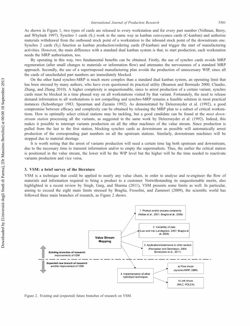
VSM is a technique that could be applied to nearly any value chain, in order to analyse and re-engineer the flow ofmaterials and information required to bring a product to a customer. Notwithstanding its unquestionable merits, alsohighlighted in a recent review by Singh, Garg, and Sharma (2011), VSM presents some limits as well. In particular,aiming to exceed the eight main limits stressed by Braglia, Frosolini, and Zammori (2009), the scientific world hasfollowed three main branches of research, as Figure 2 shows.

Figure 2. Existing and (expected) future branches of research on VSM.

International Journal of Production Research 5501

Dow

nloa

ded

by [

Uni

vers

ità d

egli

Stud

i di P

arm

a], [

Dr

Mas

sim

o B

erto

lini]

at 0

0:00

18

Sept

embe

r 20

13

A first branch of research deals with product and/or process complexity, a feature that is not covered in the standardVSM, which was initially developed for flow shop processes. For instance, Abbas, Khaswala, and Irani (2001) extendedthe applicability of VSM to HVLV manufacturing facilities, by introducing the so-called value network mapping, amapping technique that merges characteristics of VSM with production flow analysis and simplification toolkit (Iraniet al. 2000). Braglia, Carmignani, and Zammori (2006) tackled the same problem by introducing the improved VSM, aninnovative framework for the application of VSM to non-linear value streams.

In the second branch, practitioners have challenged the problem of data variability. As a matter of fact data dis-played on the current state map (CSM) are average values computed taking snapshots of the process. Still, this simpleapproach prevents a thorough comprehension of the process and so both simulation and theoretical approaches havebeen used in order to account for manufacturing variability. For instance, McDonald, Van Aken, and Rentes (2002) andLian and Van Landeghem (2007), combined VSM with discrete-event simulation, so as to answer to specific questionssuch as: the maximum level of WIP needed to support the desired takt time, the storing capacity needed by each super-market and the total flow time variability. Similarly, Braglia, Frosolini, and Zammori (2009) obtained the same answersby integrating variability analysis and VSM, so to obtain a non-static representation of the analysed value stream.

Concerning the third branch of research, several recent applications of VSM have been oriented to non-manufactur-ing environments. For example, Pavnaskar and Gersheson (2004) described differences and similarities between a pro-ductive and an engineering process and then adapted VSM to the latter one. Bonaccorsi, Carmignani, and Zammori(2011) have tailored VSM to the specific requirements of the pure services industry, by introducing new mapping iconsand operating guidelines, so as to encourage the application of VSM also in this field.

Furthermore, the authors think that another important limit of VSM lies in its narrow scope, a belief that is also con-firmed by the recent works by Serrano, Ochoa, and de Castro (2008a, 2008b). Actually, during the design of a futurestate map, VSM only considers kanban and/or CONWIP-based solutions, overlooking the possibility to employ otherPPC (such as synchro-MRP, Drum-Buffer-Rope, Workload Control and POLCA). Although kanban performs better thanMRP II, it is rather unflexible and cannot be effectively implemented in many industrial settings, such as HVLV-manu-facturing facilities (Lee 1989; Spearman, Woodruff, and Hopp 1990; Spearman and Zazanis 1992). Stevenson, Hendry,and Kingsman (2005) also assert that the optimal choice of a PPC largely depends on the production environment andso confining the system future states to a limited number of PPCs is a sub-optimal and even misleading approach.

With these premises, as shown in Figure 2, it is possible to envisage another profitable branch of research aiming toenhance and to extend VSM to the implementation of other hybrid push/pull techniques. In particular, we will presentan enlargement of VSM, from here on referred as SyVSM, which helps the analyst in considering synchro-MRP as anadditional option in the design of the FSM for a flow shop manufacturing system. Extension to more complex (i.e. jobshops) environments will be addressed in future works.

4. SyVSM for synchro-MRP: is it worth using?

VSM starts from the last workstation of the value stream and works its way back through the entire manufacturingprocess, gathering data along the way (Vinodh, Arvind, and Somanaathan 2010). At the end of the data collection step,the CSM is built. This is a graphical representation of the process, which highlights meaningful information such asflow times, WIP levels and equipment performance data, together with the information flows used to manage the physi-cal processes. This preliminary part of the analysis is straightforward and the CSM of almost every manufacturing sys-tem can be easily implemented following the basic advices given by several text books (such as Rother and Shook1999). Only in case of complex manufacturing processes, characterised by alternative routings and non-linear valuestreams, drawing the CSM could be more tackling. Still, solutions have been given also for these particular circum-stances (Irani et al. 2000; Braglia, Carmignani, and Zammori 2006) and so, with respect to the objective of the paper,the standard CSM approach can be considered adequate and will not be changed.

Conversely, a more comprehensive approach is needed when the system must proceed from the current to the futurestate. Not only because developing the FSM is a task requiring a great deal of wit and expertise, but above all becauseto avoid convergence toward kanban and CONWIP systems, the analysts should answer the following fundamentalquestions, too:

(1) Is the system under analysis suitable for synchro-MRP?(2) Do the achievable advantages justify such implementation?

A possible way to do so is detailed in the following subsections.


Dow

nloa

ded

by [

Uni

vers

ità d

egli

Stud

i di P

arm

a], [

Dr

Mas

sim

o B

erto

lini]

at 0

0:00

18

Sept

embe

r 20

13

4.1 SyVSM future state map

Answering to the first question is relatively easy. As a matter of fact, for the synchro-MRP to be superior to a standarddual kanban system, the value stream must be characterised by several product’s variants with high set-up times. Thelower the number of variants, the lower would be the inventory reduction that could be exploited blocking synchrocards. Similarly, if set-up times were negligible, then it would be possible to streamline and to level the flow (on themicro mix) using a heijunka box, without the need to either define a daily FAS or use a batch production approach.

The need to assess the suitability of SyVSM is highlighted by the fifth question of Table 1, which is a generalisationof the original guidelines proposed by Rother and Shook (1999) for the development of the FSM.

If the answer is negative, then it is not worth introducing synchro-MRP, because the increase in complexity will notbe adequately balanced by a reduction of WIP and lead times (LTs). So it is preferable to implement a pure pull system,as indicated by the original guidelines (questions from 6 to 8). Conversely, if the answer is positive, the FSM of theideal synchro-MRP system must be designed and dimensioned, following the SyVSM’s advices. To this aim, as properlyindicated by the ninth question, one has to select the critical stations that will receive the MRP production orders andthat will be used to pull production in the remaining parts of the value stream. As previously discussed, how tooptimally select those stations may be tackling, but good candidates can be found at the most downstream stations pro-cessing all the variants. Also note that, to design the SyVSM future state, guidelines (questions) 6–8 can be skipped.This is because the pacemaker process will be replaced by the critical workstations and the production of the variantswill follow a batch approach, as detailed by the MRP plan. Generally speaking, if a subset of the variants should have avery low set-up time, while producing these subset it could be possible to level production using a pacemaker processand a heijunka box. However, considering that both the pacemaker and the heijunka box could change, depending onthe variants subset being manufactured, we do not recommend this approach, as it would introduce an additional formof complexity. So our advice is to simply replace the pacemaker with the critical station(s) and let the synchro-MRPdefine the production batches.

To visualise the critical stations on the FSM, the following mapping icons can be used (Figure 3).These icons clearly show that at a critical workstation (i.e. workstation 2) production must be authorised by the

MRP plan. With a positive authorisation, production is executed, otherwise S2 cards will be pending until production(of the corresponding variant) will be re-activated.

4.2 Assessing expected WIP in the FSM

Achieving a graphical representation of the FSM is a valuable result: it forces the analyst to get an overall vision of thenew system, to detail all the physical and logical interconnection among the entities of the flow shop and to highlightpossible criticalities (i.e. bottlenecks, high set-up times, critical scheduling points, etc.). Nonetheless, to get the mostfrom SyVSM, once the FSM has been built, the expected benefits of the new process must be quantified, by computingboth the average WIP and the total flow time of the system. By doing this, one can objectively answer to question 10and ‘freeze’ the decision concerning the development of a synchro-MRP system. In case of a positive answer, the analy-sis terminates with the identification and the prioritisation of the process improvements needed to move from the actualto the future state (i.e. question 11). Otherwise synchro-MRP is discarded and a pure pull process is designed followingthe standard guidelines (6–8).

Table 1. Improved guidelines for FSM.

# Design questions Next step

1 What is the takt time? go to 22 Will production produce to a finished goods supermarket or directly to shipping? go to 33 Where can continuous flow processing be utilised? go to 44 Is there a need for a supermarket pull system within the value stream? go to 55 Is the value stream characterised by several variants? Are set-up times so relevant that

variants must be produced in large batches?IF YES go to 9 (SyVSM)ELSEgo to 6 (VSM)

6 What single point in the production chain will be used to schedule production? go to 77 How will the production mix be levelled at the pacemaker process? go to 88 What increment of work will be consistently released from the pacemaker process? go to 119 In which critical stations will synchro-MRP cards be released? go to 1010 Do expected benefits compensate the increase of control complexity? IF YES got to 11ELSE go to 611 What process improvements will be necessary? Finish


Dow

nloa

ded

by [

Uni

vers

ità d

egli

Stud

i di P

arm

a], [

Dr

Mas

sim

o B

erto

lini]

at 0

0:00

18

Sept

embe

r 20

13

Concerning this point, in case of a pure pull approach the estimation of the WIP and of the flow time is straightfor-ward. As a matter of fact, the WIP accumulating between two consecutive workstations is proportional to the number ofkanban cards used to trigger production and replenishment. Such number can be easily estimated using simple formulas,as the following one, valid in case of a fixed-order quantity (FOQ) realising policy:

Kanban Number ¼ (Average Demand During Lead Time)( 1þ k)

Containers Dimension

� �(1)

Although Equation (1) remains valid also for synchro-MRP, in this case the number of cards does not necessarilycoincide with the WIP of the system, because the production of some variants can be interrupted by the superimposedMRP-II plan. Thus, in order to answer to question 10 of Table 1, the following sub-section introduces a simple mathe-matical model to estimate the expected reduction of the on hand inventory, both under the FOQ and fixed-order interval(FOI) cards releasing policies.

4.3 Assessing expected WIP reduction of synchro-MRP

The basic quantities used in the calculation, under the hypothesis of variable production rates, deterministicreplenishment LTs and inadmissible stock outs (i.e. stock outs would halt production) are the following ones:

• OH, the average on hand inventory.

• IP, the inventory position (i.e. on hand plus outstanding orders).

• k; the average production rate.

• r; the standard deviation of the production rate.

• LT, the fixed replenishment LT.

• �q, the average replenishment quantity.

• �I ¼ �q=k, the average length of an inventory cycle (i.e. the time between two consecutive replenishmentsorders).

• r ¼ k� LT, the reorder level.

• s ¼ k(�I þ LT), the reorder up to level.

• Ss, the safety stock.

• p%, the percentage of the active production time (APT) of a generic (say ith) variant, i.e. the fraction of thetotal production time which is devoted to the production of the ith variant.

• k, the safety coefficient.

Figure 3. New mapping icons for synchro-MRP control.


Dow

nloa

ded

by [

Uni

vers

ità d

egli

Stud

i di P

arm

a], [

Dr

Mas

sim

o B

erto

lini]

at 0

0:00

18

Sept

embe

r 20

13

4.3.1 Fixed-order Quantity (FOQ)

The FOQ approach is generally used when a predetermined and fixed quantity (greater than the theoretical pitch outquantity) must be produced, in order to minimise set up times and/or other time losses. Thus we will refer to thisspecific condition from here on.

According to a FOQ policy, a fixed replenishment quantity q is ordered (i.e. �q ¼ q ¼ constant), whenever the IPdrops to r. However, in case of synchro-MRP, we must distinguish between the active and the inactive productive timeof the variant i being considered. Since the value stream produces different variants, we denote as active productive time(APT) the period when i is being manufactured and we denote as inactive production time (IPT) the period when i isnot included in the FAS, but other variants are being manufactured. Specifically, in case of synchro-MRP, an order willbe issued provided that: (i) r has been reached and (ii) the active productive time of the variant (whose IP has droppedbelow r) will last over the next inventory cycle.

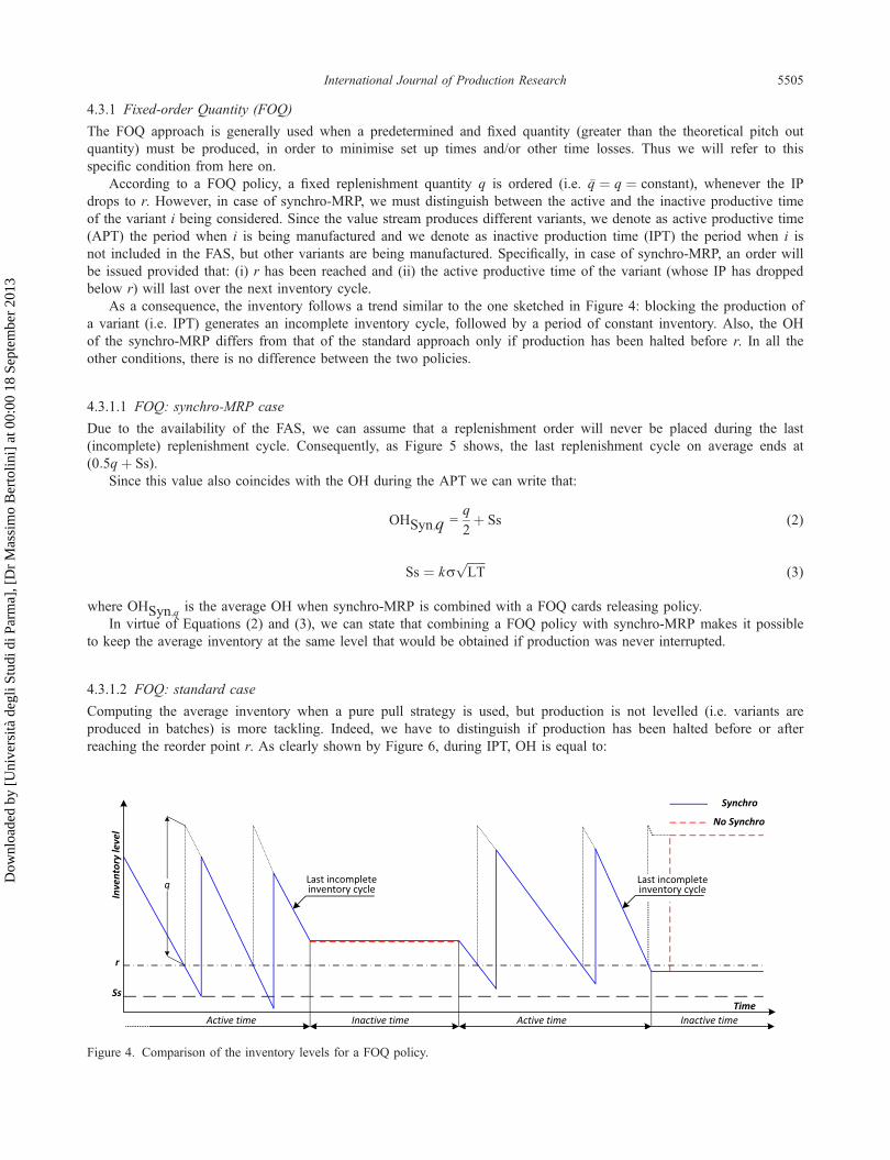
As a consequence, the inventory follows a trend similar to the one sketched in Figure 4: blocking the production ofa variant (i.e. IPT) generates an incomplete inventory cycle, followed by a period of constant inventory. Also, the OHof the synchro-MRP differs from that of the standard approach only if production has been halted before r. In all theother conditions, there is no difference between the two policies.

4.3.1.1 FOQ: synchro-MRP case

Due to the availability of the FAS, we can assume that a replenishment order will never be placed during the last(incomplete) replenishment cycle. Consequently, as Figure 5 shows, the last replenishment cycle on average ends at(0:5qþ Ss).

Since this value also coincides with the OH during the APT we can write that:

OHSyn;q =q

2þ Ss (2)

Ss ¼ krffiffiffiffiffiffiLT

p(3)

where OHSyn;q is the average OH when synchro-MRP is combined with a FOQ cards releasing policy.In virtue of Equations (2) and (3), we can state that combining a FOQ policy with synchro-MRP makes it possible

to keep the average inventory at the same level that would be obtained if production was never interrupted.

4.3.1.2 FOQ: standard case

Computing the average inventory when a pure pull strategy is used, but production is not levelled (i.e. variants areproduced in batches) is more tackling. Indeed, we have to distinguish if production has been halted before or afterreaching the reorder point r. As clearly shown by Figure 6, during IPT, OH is equal to:

Figure 4. Comparison of the inventory levels for a FOQ policy.


Dow

nloa

ded

by [

Uni

vers

ità d

egli

Stud

i di P

arm

a], [

Dr

Mas

sim

o B

erto

lini]

at 0

0:00

18

Sept

embe

r 20

13

OH ffi qþ r

2

� �if production has been halted before r

OH ffi qþr

2

� �otherwise

8<: (4)

Therefore, since OH ffi 0:5q during the APT, a rough evaluation can be obtained as follows:

OHStd;q ffi p%q

2þ (1� p%) (1� p)

qþ r

2

� �þ p qþ r

2

� �h iþ Ss (5)

where OHStd;q is the average OH for a standard FOQ cards releasing policy, p% represents the APT as a percentageof the total operating time and π is the probability to stop production after the re-order point has been reached:

p ¼ LT�I

¼ LTkq

¼ r

q(6)

Figure 6. Inventory level: FOQ policy without synchro-MRP.

Figure 5. Inventory level: FOQ policy combined with synchro-MRP.


Dow

nloa

ded

by [

Uni

vers

ità d

egli

Stud

i di P

arm

a], [

Dr

Mas

sim

o B

erto

lini]

at 0

0:00

18

Sept

embe

r 20

13

By substituting π = r/q, Equation (4) simplifies as:

OHStd;q ffi q

2þ (1� p% )r þ Ss (7)

Equation (7) can be used to compare the reduction of OH with the use of a synchro-MRP system, as shown byEquation (8).

DOHq ¼ OHStd;q � OHSyn;q ffi (1� p% )r (8)

Therefore, in virtue of Equation (8), we can state that if production (of the variants) can be halted the inventory of astandard FOQ policy diverges from the absolute minimum, as p% decreases (i.e. OH 2 ½0:5q;0:5qþ r�).

It is worth noting that Equation (7) is just a rough estimation of the real value of the average inventory. This isbecause OH depends on the length of the APT or, equivalently, on the number of consecutive replenishment cycles (n)that are being repeated without interruptions. Clearly, n cannot be considered as fixed, since it depends on the actualproduction schedule and can be changed from time to time (provided that, on average the quantity p% is respected).Nonetheless, the approximation of Equation (7) works well in most circumstances, as demonstrated in the appendix.

It is also worth mentioning that, although rather infrequently, a FOQ can be used in case of negligible set-up too. Inthis case, there are N containers (each containing q units of the item) with a card on the bottom. When a containerbecomes empty, the card is used as an order for q units. Since (N� 1) of the cards are always associated with fullcontainers, which are either in stock or ordered but not yet delivered, the inventory position is (N� 1)�q plus the num-ber of units in the container that at present is satisfying the demand. All the previously introduced equations can still beused, but first they must be ‘reinterpreted’ considering that in this case the OH is always lower than the reorder point,since r= (N� 1)� q.

4.3.2 Fixed-order Interval (FOI)

Due to its simplicity, a FOI card releasing policy is generally adopted when set-up times are not binding. According tothis policy, replenishment orders are issued with a fixed periodicity (i.e. �I ¼ I ¼ constant) and, anytime an order isplaced, a variable quantity q is ordered. Specifically, q is the minimum quantity needed to raise the IP back to a prede-termined reorder up to level (s). Thus, letting c be the capacity of each container, the quantity s/c corresponds to thetotal number of cards available in the manufacturing system.

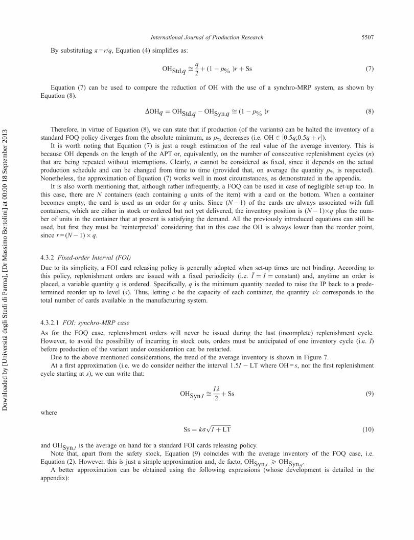
4.3.2.1 FOI: synchro-MRP case

As for the FOQ case, replenishment orders will never be issued during the last (incomplete) replenishment cycle.However, to avoid the possibility of incurring in stock outs, orders must be anticipated of one inventory cycle (i.e. I)before production of the variant under consideration can be restarted.

Due to the above mentioned considerations, the trend of the average inventory is shown in Figure 7.At a first approximation (i.e. we do consider neither the interval 1:5I � LT where OH= s, nor the first replenishment

cycle starting at s), we can write that:

OHSyn;I ffiIk2þ Ss (9)

where

Ss ¼ krffiffiffiffiffiffiffiffiffiffiffiffiffiffiI þ LT

p(10)

and OHSyn;I is the average on hand for a standard FOI cards releasing policy.Note that, apart from the safety stock, Equation (9) coincides with the average inventory of the FOQ case, i.e.

Equation (2). However, this is just a simple approximation and, de facto, OHSyn;I P OHSyn;q.A better approximation can be obtained using the following expressions (whose development is detailed in the

appendix):


Dow

nloa

ded

by [

Uni

vers

ità d

egli

Stud

i di P

arm

a], [

Dr

Mas

sim

o B

erto

lini]

at 0

0:00

18

Sept

embe

r 20

13

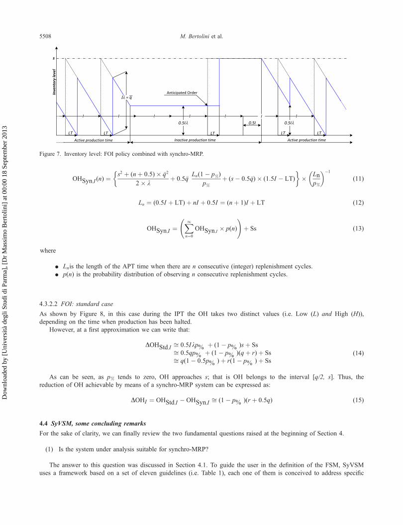
OHSyn;I (n) ¼s2 þ (nþ 0:5)� �q2

2� kþ 0:5�q

Ln(1� p%)

p%þ (s� 0:5�q)� (1:5I � LT)

� �� Ln

p%

�1

(11)

Ln ¼ (0:5I þ LT)þ nI þ 0:5I ¼ (nþ 1)I þ LT (12)

OHSyn;I ¼X1n¼0

OHSyn;I � p(n)

!þ Ss (13)

where

• Lnis the length of the APT time when there are n consecutive (integer) replenishment cycles.

• p(n) is the probability distribution of observing n consecutive replenishment cycles.

4.3.2.2 FOI: standard case

As shown by Figure 8, in this case during the IPT the OH takes two distinct values (i.e. Low (L) and High (H)),depending on the time when production has been halted.

However, at a first approximation we can write that:

DOHStd;I ffi 0:5Ikp% þ (1� p% )sþ Ssffi 0:5qp% þ (1� p% )(qþ r)þ Ssffi q(1� 0:5p% )þ r(1� p% )þ Ss

(14)

As can be seen, as p% tends to zero, OH approaches s; that is OH belongs to the interval [q/2, s]. Thus, thereduction of OH achievable by means of a synchro-MRP system can be expressed as:

DOHI ¼ OHStd;I � OHSyn;I ffi (1� p% )(r þ 0:5q) (15)

4.4 SyVSM, some concluding remarks

For the sake of clarity, we can finally review the two fundamental questions raised at the beginning of Section 4.

(1) Is the system under analysis suitable for synchro-MRP?

The answer to this question was discussed in Section 4.1. To guide the user in the definition of the FSM, SyVSMuses a framework based on a set of eleven guidelines (i.e. Table 1), each one of them is conceived to address specific

Figure 7. Inventory level: FOI policy combined with synchro-MRP.


Dow

nloa

ded

by [

Uni

vers

ità d

egli

Stud

i di P

arm

a], [

Dr

Mas

sim

o B

erto

lini]

at 0

0:00

18

Sept

embe

r 20

13

operating conditions. Specifically, the first five questions (the fifth one in particular) assess the suitability of the produc-tion system for a synchro-MRP implementation. Moreover, Table 1 guides practitioners in the design of the FSM bymeans of the new mapping icons shown in Figure 3.

(2) Do the achievable advantages justify such implementation?

Sections 4.1 and 4.2 have demonstrated how the advantages of synchro-MRP can be quantified without requiringcomplex modelling, such as discrete event simulation. In particular, a basic mathematical model to estimate the expectedreduction of the on hand inventory was presented, both under the FOQ and FOI cards releasing policies.

It is also worth noting that, unless the FSM is properly mapped via SyVSM, the use of the previously mentionedEquations (2)–(15) would be inadequate or even impossible. As a matter of fact before they can be of any use, one hasto reorganise the manufacturing process, define where (if any) U-shaped cells can be used and, most of all, identifythose point that can be used as critical workstation to stop unnecessary kanban cards. It is evident that all these preli-minary considerations are relevant part of the FSM process.

5. Industrial application

To assess the potentialities of SyVSM, an application was implemented within an electro-injectors manufacturing plant. Theplant is located in the north of Italy and is member of a larger, worldwide operating corporation. Due to reasons of industrialsecrecy, the identity of the company (from here on referred to as Electro-Injectors-Manufacturer, or EIM) must remainscreened and some data have been purposely modified, without affecting the general conclusions presented in this section.

Since long, EIM has been undertaking a lean transformation and has recently decided to implement JIT manufactur-ing for the production process of the model 4 electro-injector. Being a newly developed elector-injector mounted onhigh-performance cars, the model 4 assembly drawings cannot be shown. Nonetheless, for the purpose of this sectionwe can assimilate its structure to those of the model 1, an old injector shown in Figure 9.

The main differences concern two internally manufactured components: the lower tube and the BST needle, shownby Figures 10 and 11, respectively. The first one is a standard element obtained by welding two sub-components: thevalve body and the non-magnetic tube, a part that assures the electromagnetic decoupling of the electromagnet from theexternal body of the injector.

As for the lower tube, also the needle is obtained through the welding of three sub-components: the Ball, the Stemand the Tube (BST). This element is manufactured in three different variants differentiating both for the length and forthe diameter of the stem. Specifically, the three variants, from here on referred as ‘standard’, ‘long’ and ‘extra-long’, areproduced in accordance to the following mix: 50, 30 and 20%, respectively.

Another peculiarity of the model 4 injector is the overmold connector, which is manufactured in four differentvariants (with a mix of 60, 30, 5 and 5%) matching the different fuel rails available on the market. Since all the othercomponents are standard, the model 4 can be manufactured in 12 different variants.

Figure 8. Inventory level: FOI policy without synchro-MRP.


Dow

nloa

ded

by [

Uni

vers

ità d

egli

Stud

i di P

arm

a], [

Dr

Mas

sim

o B

erto

lini]

at 0

0:00

18

Sept

embe

r 20

13

The productive process of the model 4 is shown by the CSM of Figure 12. As it can be seen, only the lower tubeand the BST needle are internally manufactured, whereas all the other components are purchased from external suppliersand subsequently assembled in the automatic assembly shop. A washing machine is also needed to clean welded compo-nents, so as to avoid the introductions of debris and/or other contaminants that could compromise the quality of theassembly phase.

Also note that, whereas sub-components are purchased in big lots from standard suppliers, all the main model 4components are purchased from high-quality suppliers that operate accordingly to a consignment stock (CS) policy.Therefore, since the ownership of the stock is passed to EIM upon withdrawal from the CS warehouse, the possibilityof reducing both the OH of the inbound warehouse and the WIP of the value stream is an issue of primary importancefor the company, both from an economical and operating point of view, Zammori, Braglia, and Frosolini (2008).

In order to achieve this goal, the model 4 value stream has been completely re-engineered through the adoption oflean principles, as clearly shown by the FSM of Figure 13.

As can be seen from the data listed on the map, the manufacturing process has a productive capacity that (slightly)exceeds the average customers’ demand of 5500 (items/day). For this reason, it is possible to balance the value streamon the desired takt time of 5.2 (seconds/item), using a standard JIT kanban-based approach (i.e. guideline 1). Specifi-cally, this has been done by replacing buffers with supermarkets and using a single kanban system, with the exceptionof the assembly line and the washing machine that, being distantly located, have been connected by means of a dual

Figure 9. Model 1 electro-injector.

Figure 10. Lower tube.

Figure 11. BST needle.


Dow

nloa

ded

by [

Uni

vers

ità d

egli

Stud

i di P

arm

a], [

Dr

Mas

sim

o B

erto

lini]

at 0

0:00

18

Sept

embe

r 20

13

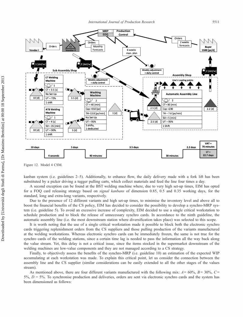
kanban system (i.e. guidelines 2–5). Additionally, to enhance flow, the daily delivery made with a fork lift has beensubstituted by a picker driving a tugger pulling carts, which collect materials and feed the line four times a day.

A second exception can be found at the BST welding machine where, due to very high set-up times, EIM has optedfor a FOQ card releasing strategy based on signal kanbans of dimension 0.85, 0.5 and 0.35 working days, for thestandard, long and extra-long variants, respectively.

Due to the presence of 12 different variants and high set-up times, to minimise the inventory level and above all toboost the financial benefits of the CS policy, EIM has decided to consider the possibility to develop a synchro-MRP sys-tem (i.e. guideline 5). To avoid an excessive increase of complexity, EIM decided to use a single critical workstation toschedule production and to block the release of unnecessary synchro cards. In accordance to the ninth guideline, theautomatic assembly line (i.e. the most downstream station where diversification takes place) was selected to this scope.

It is worth noting that the use of a single critical workstation made it possible to block both the electronic synchrocards triggering replenishment orders from the CS suppliers and those pulling production of the variants manufacturedat the welding workstations. Whereas electronic synchro cards can be immediately frozen, the same is not true for thesynchro cards of the welding stations, since a certain time lag is needed to pass the information all the way back alongthe value stream. Yet, this delay is not a critical issue, since the items stocked in the supermarket downstream of thewelding machines are low-value components and they are not managed according to a CS strategy.

Finally, to objectively assess the benefits of the synchro-MRP (i.e. guideline 10) an estimation of the expected WIPaccumulating at each workstation was made. To explain this critical point, let us consider the connection between theassembly line and the CS supplier (similar considerations can be easily extended to all the other stages of the valuesstream).

As mentioned above, there are four different variants manufactured with the following mix: A= 60%, B= 30%, C =5%, D = 5%. To synchronise production and deliveries, orders are sent via electronic synchro cards and the system hasbeen dimensioned as follows:

Figure 12. Model 4 CSM.


Dow

nloa

ded

by [

Uni

vers

ità d

egli

Stud

i di P

arm

a], [

Dr

Mas

sim

o B

erto

lini]

at 0

0:00

18

Sept

embe

r 20

13

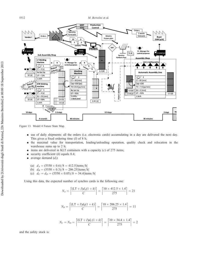
• use of daily shipments: all the orders (i.e. electronic cards) accumulating in a day are delivered the next day.This gives a fixed ordering time (I) of 8 h;

• the maximal value for transportation, loading/unloading operation, quality check and relocation in thewarehouse sums up to 2 h;

• items are delivered in KLT containers with a capacity (c) of 275 items;

• security coefficient (k) equals 0.4;

• average demand (di):

(a) dA ¼ (5550� 0:6)=8 ¼ 412:5½items=h�(b) dB ¼ (5550� 0:3)=8 ¼ 206:25½items=h�(c) dC ¼ dD ¼ (5550� 0:05)=8 ¼ 34:4½items=h�

Using this data, the expected number of synchro cards is the following one:

NA ¼ (LTþ I)dA(1þ k)

C

� �¼ 10� 412.5� 1.4

275

� �¼ 21

NB ¼ (LTþ I)dB(1þ k)

C

� �¼ 10� 206.25� 1.4

275

� �¼ 11

NC ¼ ND ¼ (LTþ I)dC(1þ k)

C

� �¼ 10� 34.4� 1.4

275

� �¼ 2

and the safety stock is:

Figure 13. Model 4 Future State Map.


Dow

nloa

ded

by [

Uni

vers

ità d

egli

Stud

i di P

arm

a], [

Dr

Mas

sim

o B

erto

lini]

at 0

0:00

18

Sept

embe

r 20

13

SsA ¼ NA � (LTþ I)dAC

¼ 21� 15 ¼ 6

SsB ¼ NB � (LTþ I)dBC

¼ 11� 7:5 ¼ 3:5

SsC ¼ SSD ¼ ND � (LTþ I)dDC

¼ 2� 1:25 ¼ 0.75

In a perfectly levelled scenario (that correspond to Equation (8)), the following level of inventory would be observedin the supermarket upstream in the assembly shop:

�QA ¼ IdA

2� Cþ SsA ¼ 6þ 6 ¼ 12KLT

�QB ¼ IdB

2� Cþ SsB ¼ 3þ 3:5 ¼ 6:5KLT

�QC ¼ �QD ¼ I � dC

2� Cþ Ssc ¼ 0:5þ 0:75 ¼ 1:25KLT

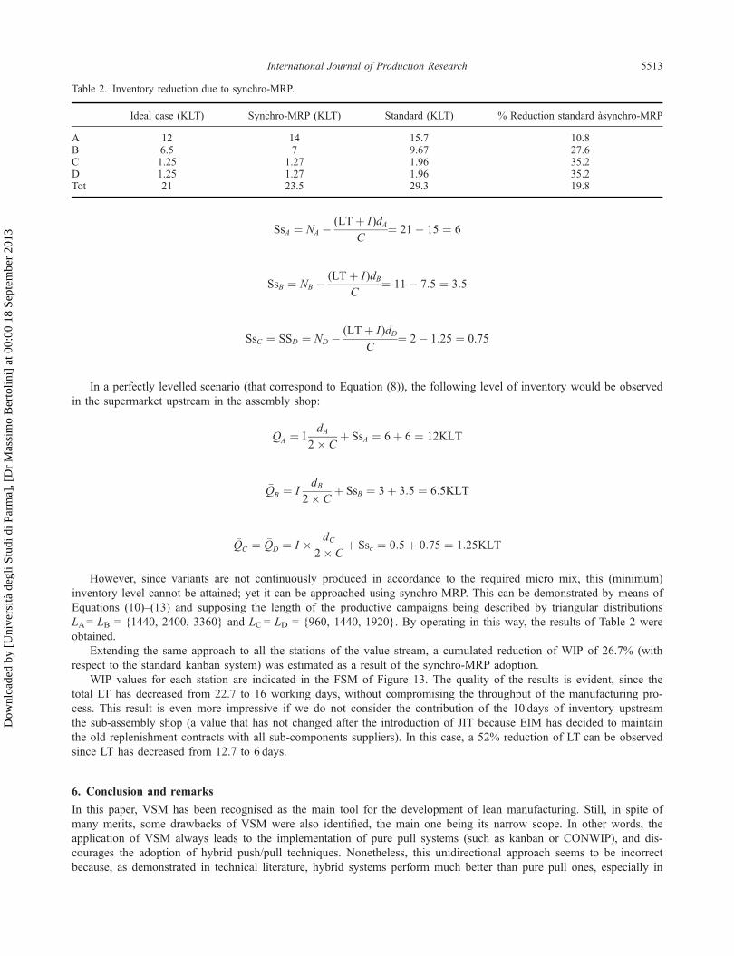
However, since variants are not continuously produced in accordance to the required micro mix, this (minimum)inventory level cannot be attained; yet it can be approached using synchro-MRP. This can be demonstrated by means ofEquations (10)–(13) and supposing the length of the productive campaigns being described by triangular distributionsLA= LB = {1440, 2400, 3360} and LC = LD = {960, 1440, 1920}. By operating in this way, the results of Table 2 wereobtained.

Extending the same approach to all the stations of the value stream, a cumulated reduction of WIP of 26.7% (withrespect to the standard kanban system) was estimated as a result of the synchro-MRP adoption.

WIP values for each station are indicated in the FSM of Figure 13. The quality of the results is evident, since thetotal LT has decreased from 22.7 to 16 working days, without compromising the throughput of the manufacturing pro-cess. This result is even more impressive if we do not consider the contribution of the 10 days of inventory upstreamthe sub-assembly shop (a value that has not changed after the introduction of JIT because EIM has decided to maintainthe old replenishment contracts with all sub-components suppliers). In this case, a 52% reduction of LT can be observedsince LT has decreased from 12.7 to 6 days.

6. Conclusion and remarks

In this paper, VSM has been recognised as the main tool for the development of lean manufacturing. Still, in spite ofmany merits, some drawbacks of VSM were also identified, the main one being its narrow scope. In other words, theapplication of VSM always leads to the implementation of pure pull systems (such as kanban or CONWIP), and dis-courages the adoption of hybrid push/pull techniques. Nonetheless, this unidirectional approach seems to be incorrectbecause, as demonstrated in technical literature, hybrid systems perform much better than pure pull ones, especially in

Table 2. Inventory reduction due to synchro-MRP.

Ideal case (KLT) Synchro-MRP (KLT) Standard (KLT) % Reduction standard àsynchro-MRP

A 12 14 15.7 10.8B 6.5 7 9.67 27.6C 1.25 1.27 1.96 35.2D 1.25 1.27 1.96 35.2Tot 21 23.5 29.3 19.8


Dow

nloa

ded

by [

Uni

vers

ità d

egli

Stud

i di P

arm

a], [

Dr

Mas

sim

o B

erto

lini]

at 0

0:00

18

Sept

embe

r 20

13

HVLV industries. For this reason, the paper presented and extended version of the standard VSM (namely SyVSM),which includes new guidelines and mapping icons that can be used to map, dimension and assess the applicability ofhybrid systems, too. We believe that the main improvement of SyVSM is summarised by the following proportion:SyVSM is to synchro-MRP as VSM is to kanban.

Finally, in order to assess the potentialities of SyVSM, an industrial application concerning electro-injectorsmanufacturing plant was presented and discussed. The results were quite impressive, as they showed a cumulated WIPreduction of 26.7% after the development of a synchro-MRP system, with peaks of WIP reductions of 35% for somecritical product’s variants.

It is intention of the authors to enlarge the analysis concerning the use of VSM as a valid tool to design and dimen-sion other PCC systems, rather than the usual kanban and CONWIP systems. By operating in this way, VSM couldovercome the traditional limits of lean production, and become a comprehensive and exhaustive manufacturing tool.

References

Abbas, Z., N. Khaswala, and S. Irani. 2001. “Value Network Mapping (VNM): Visualization and Analysis of Multiple Flows in ValueStream Maps.” Lean Management Solutions Conference, St. Louis, MO, USA.

Agrawal, N. 2010. “Review on Just in Time Techniques in Manufacturing Systems.” Advances in Production Engineering &Management 5 (2): 101–110.

Beamon, B., and J. Bermudo. 2000. “A Hybrid Push/Pull Control Algorithm for Multi-stage, Multi-line Production Systems.”Production Planning & Control 11 (4): 349–356.

Bonaccorsi, A., G. Carmignani, and F. Zammori. 2011. “Service Value Stream Management (SVSM): Developing Lean Thinking inthe Service Industry.” Journal of Service Science and Management 4 (4): 428–439.

Bonvik, A. M., C. E. Couch, and S. B. Gershwin. 1997. “A Comparison of Production-line Control Mechanisms.” InternationalJournal of Production Research 35 (3): 789–804.

Braglia, M., G. Carmignani, and F. Zammori. 2006. “A New Value Stream Mapping Approach for Complex Production Systems.”International Journal of Production Research 44 (18–19): 3929–3952.

Braglia, M., M. Frosolini, and F. Zammori. 2009. “Uncertainty in Value Stream Mapping Analysis.” International Journal of LogisticsResearch and Applications 12 (6): 435–453.

Claudio, D., J. Zhang, and Y. Zhang. 2010. “A Simulation Study for a Hybrid Inventory Control Strategy with Advance DemandInformation.” International Journal of Industrial and Systems Engineering 5 (1): 1–19.

Deleersnyder, J. L., T. J. Hodgson, R. E. King, P. J. O’Grady, and A. Savva. 1992. “Integrating Kanban Type Pull Systems and MRPType Push Systems: Insights from a Markovian Model.” IIE Transactions 24 (3): 43–56.

Emiliani, M. 2000. “Cracking the Code of Business.” Management Decision 38 (2): 60–79.Grosfeld-Nir, A., M. Magazine, and A. Vanberkel. 2000. “Push and Pull Strategies for Controlling Multistage Production Systems.”

International Journal of Production Research 38 (11): 2361–2375.Hall, R. W. 1981. Driving the Productivity Machine: Production Planning and Control in Japan. Falls Church, VA: American

Production and Inventory Control Society.Hines, P., and D. Taylor. 2000. Going Lean. Cardiff, UK: Lean Enterprise Research Centre.Hines, P., M. Holweg, and N. Rich. 2004. “Learning to Evolve: A Review of Contemporary Lean Thinking.” International Journal

of Operations & Production Management 24 (10): 994–1011.Hodgson, T. J., and D. Wang. 1991a. “Optimal Hybrid Push/Pull Control Strategies for a Parallel Multistage System: Part I.”

International Journal of Production Research 29 (6): 1279–1287.Hodgson, T. J., and D. Wang. 1991b. “Optimal Hybrid Push/Pull Control Strategies for a Parallel Multistage System: Part II.”

International Journal of Production Research 29 (7): 1453–1460.Hopp, W. J., and M. L. Spearman. 2008. Factory Physics. 3rd ed. Dubuque, IA: McGraw-Hill/Irwin.Irani, S. A., H. Zhang, J. Zhou, H. Huang, T. K. Udai, and S. Subramanian. 2000. “Production Flow Analysis and Simplification

Toolkit (PFAST).” International Journal of Production Research 38 (8): 1855–1874.Lee, L. C. 1989. “A Comparative Study of the Push and Pull Production Systems.” International Journal of Operations & Production

Management 9 (4): 5–18.Lian, Y.-H., and H. Van Landeghem. 2007. “Analysing the Effects of Lean Manufacturing Using a Value Stream Mapping-Based

Simulation Generator.” International Journal of Production Research 45 (13): 3037–3058.McDonald, T., E. M. Van Aken, and A. F. Rentes. 2002. “Utilising Simulation to Enhance Value Stream Mapping: A Manufacturing

Case Application.” International Journal of Logistics Research and Applications 5 (2): 213–232.Melton, T. 2005. “The Benefits of Lean Manufacturing.” Chemical Engineering Research and Design 83 (6): 662–673.Ohno, T. 1988. Toyota Production System – Beyond Large-Scale Production. Portland, OR: Productivity.Pavnaskar, S. J., and J. K. Gersheson. 2004. “The Application of Value Stream Mapping to Lean Engineering.” Proceedings of the

16th ASME Design Engineering Technical Conference, Salt Lake City, UT, USA.


Dow

nloa

ded

by [

Uni

vers

ità d

egli

Stud

i di P

arm

a], [

Dr

Mas

sim

o B

erto

lini]

at 0

0:00

18

Sept

embe

r 20

13

Rother, M., and J. Shook. 1999. Learning to See – Value Stream Mapping to Create Value and Eliminate Muda. Brookline, MA:Lean Enterprise Institute.

Salum, L., and Ö. U. Araz. 2009. “Using the When/Where Rules in Dual Resource Constrained Systems for a Hybrid Push-PullControl.” International Journal of Production Research 47 (6): 1661–1677.

Schonberger, R. J. 1983. “Applications of Single-Card and Dual-Card Kanban.” Interfaces 13 (4): 56–67.Serrano, I., C. Ochoa, and R. de Castro. 2008a. “An Evaluation of the Value Stream Mapping Tool.” Business Process Management

Journal 14 (1): 39–52.Serrano, I., C. Ochoa, and R. de Castro. 2008b. “Evaluation of Value Stream Mapping in Manufacturing System Redesign.”

International Journal of Production Research 46 (16): 4409–4430.Shah, R., and P. T. Ward. 2007. “Defining and Developing Measures of Lean Production.” Journal of Operations Management 25

(4): 785–805.Singh, B., S. K. Garg, and S. K. Sharma. 2011. “Value Stream Mapping: Literature Review and Implications for Indian Industry.”

International Journal of Advanced Manufacturing Technology 53 (5–8): 799–809.Spearman, M. L., and M. A. Zazanis. 1992. “Push and Pull Production Systems: Issues and Comparisons.” Operations Research 40

(3): 521–532.Spearman, M. L., D. L. Woodruff, and W. J. Hopp. 1990. “CONWIP: A Pull Alternative to Kanban.” International Journal of

Production Research 28 (5): 879–894.Stagno, A., R. Glardon, and M. Pouly. 2000. “Double Speed Single Production Line.” Journal of Intelligent Manufacturing 11 (2):

169–182.Stevenson, M., L. C. Hendry, and B. G. Kingsman. 2005. “A Review of Production Planning and Control: The Applicability of Key

Concepts to Make-to-Order Industry.” International Journal of Production Research 43 (5): 869–898.Tapping, D., T. Luyster, and T. Shuker. 2002. Value Stream Management. New York: Productivity Press.Vinodh, S., K. R. Arvind, and M. Somanaathan. 2010. “Application of Value Stream Mapping in an Indian Camshaft Manufacturing

Organisation.” Journal of Manufacturing Technology Management 21 (7): 888–900.Vollman, T. E., W. L. Berry, and D. C. Whybark. 1997. Manufacturing Planning & Control Systems . 4th ed. New York: Irwin/

McGraw Hill.Womack, J. P., and D. T. Jones. 2002. Seeing the Whole – Mapping the Extended Value Stream. Cambridge, MA: Lean Enterprise

Institute.Womack, J. P., and D. T. Jones. 2003. Lean Thinking – Banish Waste and Create Wealth in Your Corporation. 2nd ed. London: Free

Press.Zammori, F., M. Braglia, and M. Frosolini. 2008. “A Standard Agreement for Vendor Managed Inventory.” Strategic Outsourcing:

An International Journal 2 (2): 165–186.Zhang, W., and M. Chen. 2001. “A Mathematical Programming Model for Production Planning Using CONWIP.” International

Journal of Production Research 39 (12): 2723–2734.

Appendix 1

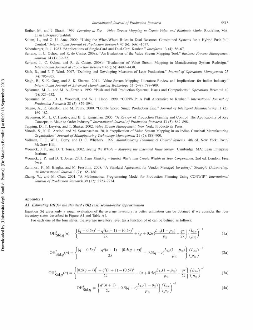
A1 Estimating OH for the standard FOQ case, second-order approximation

Equation (6) gives only a rough evaluation of the average inventory; a better estimation can be obtained if we consider the fourinventory states described in Figure A1 and Table A1.

For each one of the four states, the average inventory level (as a function of n) can be defined as follows:

OH1Std;q(n) ¼

(qþ 0:5r)2 þ q2(nþ 1)� (0:5r)2

2kþ (qþ 0:5r)

L1;n(1� p%)

p%� qr

2k

� �L1;n

p%

�1

(1a)

OH2Std;q(n) ¼

(qþ 0:5r)2 þ q2(nþ 1)� ½0:5(qþ r)�22k

þ 0:5(qþ r)L2;n(1� p%)

p%

( )L2;n

p%

�1

(2a)

OH3Std;q(n) ¼

½0:5(qþ r)�2 þ q2(nþ 1)� (0:5r)2

2kþ (qþ 0:5r)

L3;n(1� p%)

p%� qr

2k

( )L3;n

p%

�1

(3a)

OH4Std;q ¼ q2(nþ 1)

2kþ 0:5(qþ r)

L4;n(1� p%)

p%

� �L4;n

p%

�1

(4a)


Dow

nloa

ded

by [

Uni

vers

ità d

egli

Stud

i di P

arm

a], [

Dr

Mas

sim

o B

erto

lini]

at 0

0:00

18

Sept

embe

r 20

13

where Li,n is the length of the active production time of the ith configuration when there are n consecutive (integer) replenishmentcycles:

L1;n ¼ (�I þ 0:5LT)þ (nþ 1)� �I � 0:5LT ¼ (nþ 2)� �I (5a)

L2;n ¼ L3;n ¼ (�I þ 0:5LT)þ n� �I þ 0:5� (�I � LT ) ¼ (nþ 1:5)� �I (6a)

L4;n ¼ 0:5� (�I þ LT)þ n� �I þ 0:5� (�I � LT) ¼ (nþ 1)� �I (7a)

It is worth mentioning that, in each one of the four configurations we have:

limp%!0

OH1Std;q ¼ lim

p%!0OH3

Std;q ¼ (qþ 0:5r) (8a)

limp%!0

OH2Std;q ¼ lim

p%!0OH4

Std;q ¼ 0:5(qþ r) (9a)

From which it immediately follows Equation (9a).

limp%!0

OHStd;q ¼ p(qþ 0:5r)þ 0:5(1� p)(qþ r) ¼ (0:5qþ r) (10a)

Similarly, it is easy to see that:

Figure A1. Inventory level: FOQ policy without synchro-MRP system, second-order approximation.

Table A1. Inventory states: FOQ second-order approximation.

Case APT starts at APT ends at Probability

1 (HL) qþ 0:5r 0:5r p1 ¼ p2

2 (HH) qþ 0:5r 0:5� (qþ r) p ¼ p� (1� p)3 (LL) 0:5� (qþ r) 0:5r p3 ¼ p� (1� p)4 (LH) 0:5� (qþ ) 0:5� (qþ r) p4 ¼ (1� p)2


Dow

nloa

ded

by [

Uni

vers

ità d

egli

Stud

i di P

arm

a], [

Dr

Mas

sim

o B

erto

lini]

at 0

0:00

18

Sept

embe

r 20

13

limp%!1;n!1

OHStd;q ¼ q=2 (11a)

So both the minimum and the maximum value of both approximations coincide.By means of Equation (1a) to Equation (7a), the OH can be finally obtained as:

OHStd;q ¼X1n¼0

p(n)X4i¼1

(OHiStd;q(n)pi)

!þ Ss (12a)

where p(n) is the discrete probability distribution of the number of uninterrupted replenishment cycles and πi is the frequency ofoccurrence of each one of the four inventory configurations.

For what concerns p(n), we start by observing that n ¼ x if APT 2 (Tx; Txþ1� where T0 = 0 and:

Tx ¼ (xþ 1)�I þ 0:5LT; configurations 1� 2Tx ¼ (xþ 0:5)�I þ 0:5LT; configurations 3� 4

�(13a)

It is worth noting that the hypothesis is made that the active production time is equal or greater than I þ 0:5LT i.e. productioncannot be interrupted before the first inventory cycle is complete.

Also, the previous equation holds provided that 0:5LT 6 ½L4;n(1� p%)�=p%.Owing to this issue p(n) can be easily obtained by placing a probability profile f(t) (such as a triangular distribution) on the active

production time (APT) and using Equation (14a).

p(n ¼ x) ¼ZTxþ1

Tx

f (t)dt (14a)

Figure A2 shows a comparison of the outcomes of Equation (6) i.e. 1st order approximation and Equation (12a) i.e. second-orderapproximation, when q= 1000; λ= 10; LT= 45 and APT follows a triangular distribution with the following parameters [low = 200;mode =500; upper = 600].

A2 Estimating OH for the synchro FOI case, second-order approximation

Equation (15a) can be used to get a better estimate of OHSyn,I, depending on the number of consecutive replenishment cycles (n) thatare being repeated without interruptions:

580

630

680

730

780

830

880

930

980

0 0,1 0,2 0,3 0,4 0,5 0,6 0,7 0,8

OH

p%

I order approximation

II order approximation

Figure A2. Comparison between the first- and second-order approximation of OHStd,q.


Dow

nloa

ded

by [

Uni

vers

ità d

egli

Stud

i di P

arm

a], [

Dr

Mas

sim

o B

erto

lini]

at 0

0:00

18

Sept

embe

r 20

13

OHSyn;I (n) ¼s2 þ (nþ 0:5)� �q�2

2� kþ 0:5� �q� Ln � (1� p%)

p%þ (s� 0:5�q)� (1:5I � LT )

� �� Ln

p%

�1

(15a)

where, from Equation (11): Ln ¼ (0:5I þ LT)þ nI þ 0:5I ¼ (nþ 1)I þ LTPlease note that the hypothesis is made that APT P (0:5I þ LT) also, Equation (14a) holds provided that (Iþ

0:5LT) � ½L1;n(1� p%)�=p% so that the following condition is met:

limp%!0

OHSyn;I ¼ limp%!1;n!1

OHSyn;I ¼ 0:5q (16a)

It is also worth noting that, the condition limp%!0

OHSyn;I ¼ 0:5q follows from the hypothesis that (APT P (0:5I þ LT). Indeed,

due to this condition, OH equals s just for a period (1.5∙I � LT). Next OH decreases and after 2I it starts oscillating between 0 and q

until production is halted. Therefore, OHSyn,I can be considered as uniformly distributed between [0, q] during the IPT.

When p% →0, the IPT is the dominant fraction of the total available time and so limp%!0

OHSyn;I ¼ 0:5q.Clearly, if we remove the realistic hypothesis that APT P (0.5I+ LT), and assume that production can be activated also to realise

(very) small production lots, then when p%→0 OH can be considered as uniformly distributed between [0, s] and solimp%!0

OHSyn;I ¼ 0:5s.

Finally we have that:

OHSyn;I ¼X1n¼0

OHSyn;I p(n)

!þ Ss (17a)

As in the previous section, to compute p(n), we observe that n ¼ x if APT 2 (Tx;Txþ1� where T0 = 0 and:

Tx ¼ (0:5þ x)I þ LT (18a)

A3 Estimating OH for the standard FOI case, second-order approximation

As above mentioned, Equation (10) gives a rough estimation of OHStd,I. To get a better estimation, we need to consider the differentinventory states reported in Table A2.

As detailed in Section 4.3, the OH can be calculated as follows:

OH1Std;I (n) ¼

s2 þ (nþ 1)� q2 � (0:5q)2 � (0:5r)2

2� k� s� L1;n � (1� p%)

p%� 0:5� LT � (s� 0:5r)

� �L1;n

p%

�1

(19a)

OH2Std;I (n) ¼

s2 þ (nþ 1)� q2 � (0:5q)2 � (0:5s)2

2k� s� L2;n � (1� p%)

p%� 0:25� s� (I þ LT )

� �L2;n

p%

�1

(20a)

where

L1;n ¼ (LT þ 0:5I)þ (nþ 1)� I � 0:5� LT ¼ 0:5� LT þ (nþ 1:5)� I (21a)

L2;n ¼ (LTþ 0:5� I)þ (nþ 1)� I � 0:5� (I � LT) ¼ 0:5� LTþ (nþ 1)� I (22a)

It is worth noting that, for all configurations Equations (23a) and (24a) hold.

Table A2. Inventory states: FOI, second-order approximation.

Case APT starts at APT ends at Probability

1 (L) s 0:5LTk p1 ¼ p2 (H) s 0:5� (I þ LT)� k p2 ¼ 1� p


Dow

nloa

ded

by [

Uni

vers

ità d

egli

Stud

i di P

arm

a], [

Dr

Mas

sim

o B

erto

lini]

at 0

0:00

18

Sept

embe

r 20

13

limp%!0

OH1Std;I ¼ lim

p%!0OH2

Std;I ¼ s (23a)

limp%!1

OH1Std;I ¼ lim

p%!1OH2

Std;I ¼ 0:5q (24a)

And so the minimum and the maximum value of both approximations (i.e. first and second order) coincide.Finally, Equation (18a) to Equation (22a) can be summarised in Equation (25a) and we have:

OHStd;I ¼ p1 �X1n¼0

OH1Std(n)p(n)þ p2 �

X1n¼0

OH2Std(n)p(n)þ Ss (25a)

For what concerns p(n), we start by observing that n ¼ x if APT 2 (Tx;Txþ1� where T0 = 0 and:

Tx ¼ (0:5� I þ LT)þ x� I (26a)

Note that the hypothesis is made that the active production time is equal or greater than (0.5∙I + LT). Also, Equation (26a) holdsprovided that 0:5(I þ LT) 6 ½L1;n(1� p%)�=p%.

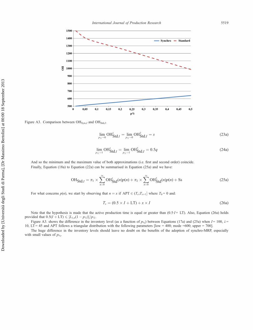
Figure A3. shows the difference in the inventory level (as a function of p%) between Equations (17a) and (25a) when I = 100, λ=10, LT= 45 and APT follows a triangular distribution with the following parameters [low = 400; mode =600; upper = 700].

The huge difference in the inventory levels should leave no doubt on the benefits of the adoption of synchro-MRP, especiallywith small values of p%.

500

600

700

800

900

1000

1100

1200

1300

1400

1500

0 0,05 0,1 0,15 0,2 0,25 0,3 0,35 0,4 0,45 0,5

OH

p%

Synchro Standard

Figure A3. Comparison between OHSyn,I and OHStd,I.


Dow

nloa

ded

by [

Uni

vers

ità d

egli

Stud

i di P

arm

a], [

Dr

Mas

sim

o B

erto

lini]

at 0

0:00

18

Sept

embe

r 20

13

aMassimo Bertolini , Marcello Braglia , Giovanni … · Extending value stream mapping: the...

Documents

Transcript of aMassimo Bertolini , Marcello Braglia , Giovanni … · Extending value stream mapping: the...