arX

iv:a

stro

-ph/

0505

266v

2 1

Aug

200

5

Alternatives to Dark Matter and Dark Energy

Philip D. Mannheim

Department of Physics, University of Connecticut, Storrs, CT 06269, USAemail: philip.mannheim@uconn.edu

July 28, 2005

Abstract

We review the underpinnings of the standard Newton-Einstein theory of gravity, and identifywhere it could possibly go wrong. In particular, we discuss the logical independence from eachother of the general covariance principle, the equivalence principle and the Einstein equations, anddiscuss how to constrain the matter energy-momentum tensor which serves as the source of gravity.We identify the a priori assumption of the validity of standard gravity on all distance scales as theroot cause of the dark matter and dark energy problems, and discuss how the freedom currentlypresent in gravitational theory can enable us to construct candidate alternatives to the standardtheory in which the dark matter and dark energy problems could then be resolved. We identifythree generic aspects of these alternate approaches: that it is a universal acceleration scale whichdetermines when a luminous Newtonian expectation is to fail to fit data, that there is a globalcosmological effect on local galactic motions which can replace galactic dark matter, and that tosolve the cosmological constant problem it is not necessary to quench the cosmological constantitself, but only the amount by which it gravitates.

1 Introduction

Following many years of research in cosmology and astrophysics, a picture of the universe has emerged[1, 2, 3, 4, 5] which is as troubling as it is impressive. Specifically, a wide variety of data currentlysupport the view that the matter content of the universe consists of two primary components, viz. darkmatter and dark energy, with ordinary luminous matter being relegated to a decidedly minor role. Thenature and composition of these dark matter and dark energy components is not at all well-understood,and while both present severe challenges to the standard theory, each presents a different kind ofchallenge to it. As regards dark matter, there is nothing in principle wrong with the existence of non-luminous material per se (indeed objects such as dead stars, brown dwarfs and massive neutrinos arewell-established in nature). Rather, what is disturbing is the ad hoc, after the fact, way in which darkmatter is actually introduced, with its presence only being inferred after known luminous astrophysicalsources are found to fail to account for any given astrophysical observation. Dark matter thus seems toknow where, and in what amount, it is to be needed, and to know when it is not in fact needed (darkmatter has to avoid being abundant in the solar system in order to not impair the success of standardgravity in accounting for solar system observations using visible sources alone); and moreover, in thecases where it is needed, what it is actually made of (astrophysical sources (Machos) or new elementaryparticles (Wimps)) is as yet totally unknown and elusive.

1

Disturbing as the dark matter problem is, the dark energy problem is even more severe, and notsimply because its composition and nature is as mysterious as that of dark matter. Rather, for darkenergy there actually is a very good, quite clear-cut candidate, viz. a cosmological constant, and theproblem here is that the value for the cosmological constant as anticipated from fundamental theoryis orders of magnitude larger than the data can possibly permit. With dark matter then, we seethat luminous sources alone underaccount for the data, while for dark energy, a cosmological constantoveraccounts for the data. Thus, within the standard picture, arbitrary as their introduction might be,there is nonetheless room for dark matter candidates should they ultimately be found, but for darkenergy there is a need not to find something which might only momentarily be missing, but rather toget rid of something which is definitely there. And indeed, if it does not prove possible to quench thecosmological constant by the requisite orders and orders of magnitude, one would have to conclude thatthe prevailing cosmological theory simply does not work.

In arriving at the predicament that contemporary astrophysical and cosmological theory thus findsitself in, it is important to recognize that the entire case for the existence of dark matter and darkenergy is based on just one thing alone, viz. on the validity on all distance scales of the standardNewton-Einstein gravitational theory as expressed through the Einstein equations of motion

−c3

8πG

(

Rµν −1

2gµνRα

α

)

= T µν (1)

for the gravitational field gµν . Specifically, the standard approach to cosmology and astrophysics is totake the Einstein equations of motion as given, and whenever the theory is found to encounter observa-tional difficulties on any particular distance scale, modifications are to then be made to T µν through theintroduction of new, essentially ad hoc, gravitational sources so that agreement with observation canthen be restored. While a better understanding of dark energy and explicit observational detection ofdark matter sources might eventually be achieved in the future, at the present time the only apparentway to avoid the dark matter and dark energy problems is to modify or generalize not the right-handside of Eq. (1) but rather its left. In order to see how one might actually do this, it is thus necessary tocarefully go over the entire package represented by Eq. (1), to determine whether some of its ingredientsmight not be as secure as others, and investigate whether the weaker ones could possibly be replaced.To do this we will thus need to make a critical appraisal of both of the two sides of Eq. (1).

2 The underpinnings of the standard gravitational picture

2.1 Massive test particle motion

Following a year of remarkable achievement, achievement whose centennial is currently being celebrated,at the end of 1905 Einstein found himself in a somewhat paradoxical situation. While he had surmountedan enormous hurdle in developing special relativity, its very establishment created an even bigger hurdlefor him. Specifically, with the development of special relativity Einstein resolved the conflict betweenthe Lorentz invariance of the Maxwell equations and the Galilean invariance of Newtonian mechanicsby realizing that it was Lorentz invariance which was the more basic of the two principles, and that itwas Newtonian mechanics which therefore had to be modified. While special relativity thus ascribedprimacy to Lorentz invariance so that observers moving with large or small uniform velocity could thenall agree on the same physics, such observers still occupied a highly privileged position since uniformvelocity observers form only a very small subset of all possible allowable observers, observers who couldmove with arbitrarily non-uniform velocity. Additionally, if it was special relativity that was to be theall-embracing principle, all interactions would then need to obey it, and yet what was at the time theaccepted theory of gravity, viz. Newtonian gravity, in fact did not. It was the simultaneous resolution

2

of these two issues (viz. accelerating observers and the compatibility of gravity with relativity) at oneand the same time through the spectacular development of general relativity which not only establishedthe Einstein theory of gravity, but which left the impression that there was only one possible resolutionto the two issues, viz. that based on Eq. (1). To pinpoint what it is in the standard theory which leadsus to the dark matter and dark energy problems, we thus need to unravel the standard gravitationalpackage into what are in fact logically independent components, an exercise which is actually of valuein and of itself regardless in fact of the dark matter and dark energy problems.

In order to make such a dissection of the standard picture, we begin with a discussion of a standard,free, spinless, relativistic, classical-mechanical Newtonian particle of non-zero kinematic mass m movingin flat spacetime according to the special relativistic generalization of Newton’s second law of motion

md2ξα

dτ 2= 0 , Rµνστ = 0 , (2)

where dτ = (−ηαβdξαdξβ)1/2 is the proper time and ηαβ is the flat spacetime metric, and where we

have indicated explicitly that the Riemann tensor is (for the moment) zero. As such, Eq. (2) will beleft invariant under linear transformations of the coordinates ξµ, but on making an arbitrary non-lineartransformation to coordinates xµ and using the definitions

Γλµν =∂xλ

∂ξα∂2ξα

∂xµ∂xν, gµν =

∂ξα

∂xµ∂ξβ

∂xνηαβ , (3)

we directly find (see e.g. [6], a reference whose notation we use throughout) that the invariant propertime is brought to the form dτ = (−gµνdx

µdxν)1/2, and that the equation of motion of Eq. (2) isrewritten as

m

(

D2xλ

Dτ 2

)

≡ m

(

d2xλ

dτ 2+ Γλµν

dxµ

dτ

dxν

dτ

)

= 0 , Rµνστ = 0 , (4)

with Eq. (4) serving to defineD2xλ/Dτ 2. As derived, Eq. (4) so far only holds in a strictly flat spacetimewith zero Riemann curvature tensor, and indeed Eq. (4) is only a covariant rewriting of the specialrelativistic Newtonian second law of motion, i.e. it covariantly describes what an observer with a non-uniform velocity in flat spacetime sees, with the Γλµν term emerging as an inertial, coordinate-dependentforce. The emergence of such a Γλµν term originates in the fact that even while the four-velocity dxλ/dτtransforms as a general contravariant vector, its ordinary derivative d2xλ/dτ 2 (which samples adjacentpoints and not merely the point where the four-velocity itself is calculated) does not, and it is only thefour-acceleration D2xλ/Dτ 2 which transforms as a general contravariant four-vector, and it is thus onlythis particular four-vector on whose meaning all (accelerating and non-accelerating) observers can agree.The quantity Γλµν is not itself a general coordinate tensor, and in flat spacetime one can eliminate iteverywhere by working in Cartesian coordinates. Despite this privileged status for Cartesian coordinatesystems, in general it is Eq. (4) rather than Eq. (2) which should be used (even in flat spacetime) sincethis is the form of Newton’s second law of motion which an accelerating flat spacetime observer sees.

Now while all of the above remarks where developed purely for flat spacetime, Eq. (4) has animmediate generalization to curved spacetime where it then takes the form

m

(

D2xλ

Dτ 2

)

≡ m

(

d2xλ

dτ 2+ Γλµν

dxµ

dτ

dxν

dτ

)

= 0 , Rµνστ 6= 0 . (5)

In curved spacetime, it is again only the quantity D2xλ/Dτ 2 which transforms as a general contravariantfour-vector, and the Christoffel symbol Γλµν is again not a general coordinate tensor. Consequently atany given point P it can be made to vanish,1 though no coordinate transformation can bring it to zero

1Under the transformation x′λ = xλ + 12x

µxν(Γλµν)P , the primed coordinate Christoffel symbols (Γ′λµν)P will vanish at

the point P , regardless in fact of how large the Riemann tensor in the neighborhood of the point P might actually be.

3

at every point in a spacetime whose Riemann tensor is non-vanishing. As an equation, Eq. (5) can alsobe obtained from an action principle, since it is the stationarity condition δIT/δxλ = 0 associated withfunctional variation of the test particle action

IT = −mc∫

dτ (6)

with respect to the coordinate xλ. To appreciate the ubiquity of the appearance of the covariantacceleration D2xλ/Dτ 2, we consider as action the curved space electromagnetic coupling

I(2)T = −mc

∫

dτ + e∫

dτdxλ

dτAλ , (7)

to find that its variation with respect to xλ leads to the curved space Lorentz force law

mc

(

d2xλ

dτ 2+ Γλµν

dxµ

dτ

dxν

dτ

)

= eF λα

dxα

dτ, Rµνστ 6= 0 . (8)

Similarly, the coupling of the test particle to the Ricci scalar via

I(3)T = −mc

∫

dτ − κ∫

dτRαα , (9)

leads to

(mc + κRαα)

(

d2xλ

dτ 2+ Γλµν

dxµ

dτ

dxν

dτ

)

= −κRαα;β

(

gλβ +dxλ

dτ

dxβ

dτ

)

, (10)

(Rµνστ necessarily non-zero here), while the coupling of the test particle to a scalar field S(x) via

I(4)T = −κ

∫

dτS(x) , (11)

leads to the curved space

κS

(

d2xλ

dτ 2+ Γλµν

dxµ

dτ

dxν

dτ

)

= −κS;β

(

gλβ +dxλ

dτ

dxβ

dτ

)

, Rµνστ 6= 0 , (12)

an expression incidentally which reduces to Eq. (5) when S(x) is a spacetime constant (with the massparameter then being given by mc = κS). In all of the above cases then it is the quantity D2xλ/Dτ 2

which must appear, since in each such case the action which is varied is a general coordinate scalar.

2.2 The equivalence principle

Now as such, the analysis given above is a purely kinematic one which discusses only the propagation oftest particles in curved backgrounds. This analysis makes no reference to gravity per se, and in particularmakes no reference to Eq. (1) at all, though it does imply that in any curved spacetime in which the met-ric gµν is taken to be the gravitational field, covariant equations of motion involving four-accelerationswould have to based strictly on D2xλ/Dτ 2, with neither d2xλ/dτ 2 nor Γλµν(dx

µ/dτ)(dxν/dτ) having anycoordinate independent significance or meaning. As such, we thus recognize the equivalence principleas the statement that the d2xλ/dτ 2 and Γλµν(dx

µ/dτ)(dxν/dτ) terms must appear in all of the abovepropagation equations in precisely the combination indicated,2 and that via a coordinate transformationit is possible to remove the Christoffel symbols at any chosen point P , with it thereby being possible to

2This thereby secures the equality of the inertial and passive gravitational masses of material particles.

4

simulate the Christoffel symbol contribution to the gravitational field at such a point P by an acceler-ating coordinate system in flat spacetime. We introduce this particular formulation of the equivalenceprinciple quite guardedly, since in an equation such as the fully covariant Eq. (10), one cannot removethe dependence on the Ricci scalar by any coordinate transformation whatsoever, and we thus define theequivalence principle not as the statement that all gravitational effects at any point P can be simulatedby an accelerating coordinate system in flat spacetime (viz. that test particles unambiguously move ongeodesics and obey Eq. (5) and none other), but rather that no matter what propagation equation isto be used for test particles, the appropriate acceleration for them is D2xλ/Dτ 2.3 With Eq. (4) thusshowing the role of coordinate invariance in flat spacetime, with Eqs. (5), (8), and (10) exhibiting theequivalence principle in curved spacetime, and with all of these equations being independent of the Ein-stein equations of Eq. (1), the logical independence of the general covariance principle, the equivalenceprinciple and the Einstein equations is thus established. Hence, any metric theory of gravity in whichthe action is a general coordinate scalar and the metric is the gravitational field will thus automaticallyobey both the relativity principle and the equivalence principle, no matter whether or not the Einsteinequations are to be imposed as well.4

2.3 Massless field motion

Absent from the above discussion is the question of whether real, as opposed to test, particles actuallyobey curved space propagation equations such as Eq. (5) at all, and whether such a discussion shouldapply to massless particles as well since for them both m and the proper time dτ vanish identically,with equations such as Eq. (5) becoming meaningless. Now it turns out that these two issues arenot actually independent, as both reduce to the question of how waves rather than particles couple togravity, since light is described by a wave equation, and elementary particles are actually taken to bethe quanta associated with quantized fields which are also described by wave equations. And since thediscussion will be of relevance for the exploration of the energy-momentum tensor to be given below,we present it in some detail now. For simplicity we look at the standard minimally coupled curvedspacetime massless Klein-Gordon scalar field with wave equation

S ;µ;µ = 0 , Rµνστ 6= 0 (13)

where S ;µ denotes the contravariant derivative ∂S/∂xµ. If for the scalar field we introduce a eikonalphase T (x) via S(x) = exp(iT (x)), the scalar T (x) is then found to obey the equation

T ;µT;µ − iT ;µ;µ = 0 , (14)

3This particular formulation of the equivalence principle does no violence to observation, since Eotvos experiment typetesting of the equivalence principle is made in Ricci-flat Schwarzschild geometries where all Ricci tensor or Ricci scalardependent terms (such as for instance those exhibited in Eq. (10)) are simply absent, with such tests (and in fact anywhich involve the Schwarzschild geometry) not being able to distinguish between Eqs. (4) and (10).

4To sharpen this point, we note that it could have been the case that the resolution of the conflict between gravityand special relativity could have been through the introduction of the gravitational force not as a geometric entity atall, but rather as an analog of the way the Lorentz force is introduced in Eq. (8). In such a case, in an acceleratingcoordinate system one would still need to use the acceleration D2xλ/Dτ2 and not the ordinary d2xλ/dτ2. However, ifthe gravitational field were to be treated the same way as the electromagnetic field, left open would then be the issue ofwhether physics is to be conducted in flat space or curved space, i.e. left open would be the question of what does thenfix the Riemann tensor. There would then have to be some additional equation which would fix it, and curvature wouldstill have to be recognized as having true, non-coordinate artifact effects on particles if the Riemann tensor were thenfound to be non-zero. Taking such curvature to be associated with the gravitational field (rather than with some furtherfield) is of course the most economical, though doing so would not oblige gravitational effects to only be felt throughD2xλ/Dτ2, and would not preclude some gravitational Lorentz force type term (such as the one exhibited in Eq. (10))from appearing as well.

5

an equation which reduces to T ;µT;µ = 0 in the short wavelength limit. From the relation T ;µT;µ;ν = 0which then ensues, it follows that in the short wavelength limit the phase T (x) obeys

T ;µT;µ;ν = T ;µ[T;ν;µ + ∂νT;µ − ∂µT;ν ] = T ;µ[T;ν;µ + ∂ν∂µT − ∂µ∂νT ] = T ;µT;ν;µ = 0 . (15)

Since normals to wavefronts obey the eikonal relation

T ;µ =dxµ

dq= kµ (16)

where q is a convenient scalar affine parameter which measures distance along the normals and kµ isthe wave vector of the wave, on noting that (dxµ/dq)(∂/∂xµ) = d/dq we thus obtain

kµkλ;µ =d2xλ

dq2+ Γλµν

dxµ

dq

dxν

dq= 0 , (17)

a condition which we recognize as being the massless particle geodesic equation, with rays then preciselybeing found to be geodesic in the eikonal limit. Since the discussion given earlier of the coordinatedependence of the Christoffel symbols was purely geometric, we thus see that once rays such as lightrays are geodesic, they immediately obey the the equivalence principle,5 with phenomena such as thegravitational bending of light then immediately following.

Now while we do obtain strict geodesic motion for rays when we eikonalize the minimally cou-pled Klein-Gordon equation, the situation becomes somewhat different if we consider a non-minimallycoupled Klein-Gordon equation instead. Thus, on replacing Eq. (13) by

S ;µ;µ +

ξ

6SRα

α = 0 , Rµνστ 6= 0 , (18)

the curved space eikonal equation then takes the form

T ;µT;µ −ξ

6Rα

α = 0 , (19)

with Eq. (17) being replaced by the Ricci scalar dependent

d2xλ

dq2+ Γλµν

dxµ

dq

dxν

dq=

ξ

12(Rα

α);λ (20)

in the short wavelength limit.A similar dependence on the Ricci scalar or tensor is also obtained for massless spin one-half and

spin one fields. Specifically, even though the massless Dirac equation in curved space, viz. iγµ(x)[∂µ +Γµ]ψ(x) = 0 (where Γµ(x) is the fermion spin connection) contains no explicit direct dependenceon the Ricci tensor, nonetheless the second order differential equation which the fermion field thenalso obeys is found to take the form [∂µ + Γµ][∂

µ + Γµ]ψ(x) + (1/4)Rααψ(x) = 0. Likewise, even

though the curved space Maxwell equations, viz. F µν;ν = 0, Fµν;λ + Fλµ;ν + Fνλ;µ = 0 also possess no

direct coupling to the Ricci tensor, manipulation of the Maxwell equations leads to the second ordergαβF µν

;α;β+FµαRν

α−FναRµ

α = 0, and thus to the second order equation gαβAµ;α;β−Aα;α;µ+A

αRµα = 0for the vector potential Aµ. Characteristic of all these massless field equations then is the emergenceof an explicit dependence on the Ricci tensor, and thus of some non-geodesic motion analogous tothat exhibited in Eq. (20) when we eikonalize.6 Now equations such as Eq. (20) will still obey the

5According to Eq. (17), an observer in Einstein’s elevator would not be able to tell if a light ray is falling downwardsunder gravity or whether the elevator is accelerating upwards.

6We note that none of these particular curved space field equations involve the Riemann tensor, but only the Riccitensor. This is fortunate since Schwarzschild geometry tests of gravity would be sensitive to the Riemann tensor, a tensorwhich in contrast to the Ricci tensor, does not vanish in a Schwarzschild geometry.

6

equivalence principle (as we have defined it above), since the four-acceleration which appears is still onewhich contains the non-tensor Christoffel symbols. Moreover, despite the fact that all of these particularcurved space equations are non-geodesic, nonetheless, in the flat space limit all of them degenerateinto the flat space geodesics, with the eikonal rays travelling on straight lines. Now in general, what isunderstood by covariantizing is to replace flat spacetime expressions by their curved space counterparts,with Eq. (4) for instance being replaced by Eq. (5). However, this is a very restrictive procedure, sinceEqs. (5) and (10) both have the same flat space limit. The standard covariantizing prescription willthus fail to generate any terms which explicitly depend on curvature (terms which in some cases we seemust be there), and thus constructing a curved space energy-momentum tensor purely by covariantizinga flat space one is not at all a general prescription, a issue we shall return to below when we discussthe curved space energy-momentum tensor in detail.

2.4 Massive field motion

A situation analogous to the above also obtains for massive fields. Specifically for the quantum-mechanical minimally coupled curved space massive Klein-Gordon equation, viz.

S ;µ;µ −

m2c2

h2 S = 0 , Rµνστ 6= 0 , (21)

the substitution S(x) = exp(iP (x)/h) yields

P ;µP;µ +m2c2 = ihP ;µ;µ . (22)

In the eikonal (or the small h) approximation the ihP µ;µ term can be dropped, so that the phase P (x)

is then seen to obey the purely classical condition

gµνP;µP ;ν +m2c2 = 0 . (23)

We immediately recognize Eq. (23) as the covariant Hamilton-Jacobi equation of classical mechanics,an equation whose solution is none other than the stationary classical action

∫

pµdxµ as evaluated

between relevant end points. In the eikonal approximation then we can thus identify the wave phaseP (x) as

∫

pµdxµ, with the phase derivative P ;µ = ∂µP then being given as the particle momentum

pµ = mcdxµ/dτ , a four-vector momentum which accordingly has to obey

gµνpµpν +m2c2 = 0 , (24)

the familiar fully covariant particle energy-momentum relation. With covariant differentiation of Eq.(24) immediately leading to the classical massive particle geodesic equation

pµpλ;µ =d2xλ

dτ 2+ Γλµν

dxµ

dτ

dxν

dτ= 0 (25)

(as obtained here with the proper time dτ appropriate to massive particles and not the affine parameterq), we thus recover the well known result that the center of a quantum-mechanical wave packet followsthe stationary classical trajectory. Further, since we may also reexpress the stationary

∫

pµdxµ as

−mc∫

dτ , we see that we can also identify the quantum-mechanical eikonal phase as P (x) = −mc∫

dτ ,to thus enable us to make contact with the IT action given in Eq. (6).7 Though we have thus madecontact with IT , it is important to realize that we were only able to arrive at Eq. (23) after havingstarted with the equation of motion of Eq. (21), an equation whose own validity requires that stationary

7We make contact with the IT of Eq. (6) since we start with the minimally coupled Eq. (21).

7

variation of the Klein-Gordon action from which it is derived had already been made, with only thestationary classical action actually being a solution to the Hamilton-Jacobi equation. The action IT =−mc

∫

dτ as evaluated along the stationary classical path is thus a part of the solution to the waveequation, i.e. the output, rather than a part of the input.8 Thus in the quantum-mechanical case wenever need to assume as input the existence of any point particle action such as IT at all. Rather,we need only assume the existence of equations such as the standard Klein-Gordon equation, witheikonalization then precisely putting particles onto classical geodesics just as desired. To conclude then,we see that not only does the equivalence principle hold for light (even though it has no inertial mass orgravitational mass at all) and hold for quantum-mechanical particles, we also see that the equivalenceprinciple need not be intimately tied to the classical test particle action IT at all. Given this analysis,we turn now to consideration of the curved space energy-momentum tensor.

3 Structure of the energy-momentum tensor

3.1 Kinematic perfect fluids

At the time of the development of general relativity, the prevailing view of gravitational sources wasthat they were to be treated like billiard balls, i.e. as purely mechanical kinematic particles whichcarry energy and momentum; with the advent of general relativity then requiring that such energy andmomentum be treated covariantly, so that the way the energy-momentum tensor was to be introducedin gravitational theory was to simply covariantize the appropriate flat spacetime expressions. Despitethe subsequent realization that particles are very far from being such kinematic objects (elementaryparticles are now thought to get their masses dynamically via spontaneous symmetry breaking), anddespite the fact that the now standard SU(3)×SU(2)×U(1) theory of strong, electromagnetic and weakinteractions ascribes primacy to fields over particles, the kinematically prescribed energy-momentumtensor (rather than an SU(3)×SU(2)×U(1) based one) is nonetheless still used in treatments of gravitytoday. Apart from this already disturbing shortcoming (one we shall remedy below by constructing theenergy-momentum tensor starting from fields rather than particles), an additional deficiency of a purelykinematic prescription is that since flat spacetime energy-momentum tensors had no need to know wherethe zero of energy was (in flat spacetime only energy differences are observable), their covariantizing leftunidentified where the zero of energy might actually be; and since gravity couples to energy itself ratherthan to energy differences, this kinematic prescription is thus powerless to address the cosmologicalconstant problem, an issue to which we shall return below.

Historically there was of course good reason to treat particles kinematically, since such a treatmentdid lead to geodesic motion for the particles. Thus for the test particle action IT of Eq. (6), its functionalvariation with respect to the metric allows one to define an energy-momentum tensor according to9

2

(−g)1/2

δITδgµν

= T µν =mc

(−g)1/2

∫

dτδ4(x− y(τ))dyµ

dτ

dyν

dτ, (26)

with its covariant conservation (T µν;ν = 0) leading right back to the geodesic equation of Eq. (5).10

Moreover, an analogous situation is met when the energy-momentum tensor is taken to be a perfect8Thus we cannot appeal to IT to put particles on geodesics, since we already had to put them on the geodesics which

follow from Eq. (23) in order to get to IT in the first place. While the use of an action such as IT will suffice to obtaingeodesic motion, as we thus see, its use is not at all necessary, with it being eikonalization of the quantum-mechanicalwave equation which actually puts massive particles on geodesics.

9With our definition here and throughout of T µν as T µν = 2(δIT /δgµν)/(−g)1/2, it is cT00 which then has the dimensionof an energy density rather than T00 itself.

10While our ability to impose a conservation condition on T µν would follow from Eq. (1) since the Einstein tensorGµν = Rµν − (1/2)gµνRα

α obeys the Bianchi identity, the use of a conservation condition in no way requires the validityof Eq. (1). Specifically, in any covariant theory of gravity in which the pure gravitational piece of the action, IGRAV ,

8

fluid of the form

T µν =1

c[(ρ+ p)UµUν + pgµν ] (27)

with energy density ρ, pressure p and a fluid four-vector which is normalized to UµUµ = −1. Specifically,

for such a fluid, covariant conservation leads to

[(ρ+ p)UµUν + pgµν ];ν = [(ρ+ p)Uν ];νUµ + (ρ+ p)Uµ

;νUν + p;µ = 0 , (28)

and thus to− [(ρ+ p)Uν ];ν + Uµp

;µ = −(ρ+ p)Uµ;νU

νUµ = 0 , (29)

with the last equality following since UµUµ;ν = 0. With the insertion of Eq. (29) into (28) then yielding

(ρ+ p)Uµ;νU

ν + p;ν [gµν + UµUν ] = 0 , (30)

viz.D2xµ

Dτ 2= −[gµν + UµUν ]

p;ν

(ρ+ p), (31)

we see that the geodesic equation then emerges whenever the right-hand side of Eq. (31) is negligible,a situation which is for instance met when the fluid is composed of non-interacting pressureless dust.

Since Eqs. (26) and (31) do lead to geodesic motion, it is generally thought that gravitationalsources should thus be described in this way. However, even within an a priori kinematic perfect fluidframework, Eq. (31) would in no way need to be altered if to the perfect fluid of Eq. (27) we wereto add an additional T µνEXTRA which was itself independently covariantly conserved. Since a geometrictensor such as the Einstein tensor Gµν is both covariantly conserved and non-existent in flat spacetime,a curved space generalization of a flat space energy-momentum tensor which would include a term ofthe form T µνEXTRA = Gµν would not affect Eq. (31) at all. Moreover, since the metric tensor gµν is alsocovariantly conserved, the inclusion in T µνEXTRA of a Λgµν term with Λ constant would also leave Eq.(31) untouched, and while such a term would not vanish in the flat spacetime limit, its presence in flatspacetime would only lead to a non-observable overall shift in the zero of energy. Restricting to theperfect fluid of Eq. (27) is thus only sufficient to recover Eq. (31), and not at all necessary.

Within the kinematic perfect fluid framework, the use of such fluids as gravitational sources is greatlyfacilitated if some equation of state of the form p = wρ can be prescribed where w would be a constant.To see what choices are suggested for w from flat space physics, we consider a relativistic flat spaceideal N particle classical gas of particles of mass m in a volume V at a temperature T . For this systemthe Helmholtz free energy A(V, T ) is given as

e−A(V,T )/NkT = V∫

d3pe−(p2+m2)1/2/kT , (32)

so that the pressure takes the simple form

P = −

(

∂A

∂V

)

T

=NkT

V, (33)

while the internal energy U = ρV evaluates in terms of Bessel functions as

U = A− T

(

∂A

∂T

)

V

= 3NkT +NmK1(m/kT )

K2(m/kT ). (34)

is a general coordinate scalar function of the metric, the quantity Aµν = (2/(−g)1/2)(δIGRAV /δgµν) will, because ofcovariance, automatically obey Aµν

;ν = 0, and through the gravitational equation of motion Aµν = T µν then lead tothe covariant conservation of T µν . The use of the Einstein equations is only sufficient to yield T µν

;ν = 0, but not at allnecessary, with the conservation ensuing in any general covariant pure metric theory of gravity.

9

In the high and low temperature limits (the radiation and matter eras) we then find that the expressionfor U simplifies to

U

V→

3NkT

V= 3P ,

m

kT→ 0 ,

U

V→

Nm

V+

3NkT

2V=Nm

V+

3P

2≈Nm

V,

m

kT→ ∞ . (35)

Consequently, while p and ρ are nicely proportional to each other in the high temperature radiationand the low temperature matter eras (where w(T → ∞) = 1/3 and w(T → 0) = 0), we also see thatin transition region between the two eras their relationship is altogether more complicated. Use of ap = wρ equation of state would at best only be valid at temperatures which are very different fromthose of order m/K, though for massless particles it would be of course be valid to use p = ρ/3 at alltemperatures, a point to which we shall return below.

3.2 Perfect Robertson-Walker fluids

In trying to develop equations of state in curved space, one should replace the partition function inEq. (32) by its curved space generalization (i.e. one should covariantize it, just as is proposed forT µν itself),11 and then follow the steps above to see what generalization of Eq. (35) might then ensue.However for curved backgrounds of high symmetry, the use of the isometry structure of the backgroundcan greatly simplify the discussion. Thus, for instance, for the Robertson-Walker geometry of relevanceto cosmology, viz.

ds2 = −c2dt2 +R2(t)

(

dr2

(1 − kr2)+ r2dΩ2

)

, (36)

the maximal 3-symmetry of the background entails that any rank two tensor such as the energy-momentum tensor itself must have the generic form

T µν = [C(t) +D(t)]UµUν +D(t)gµν , (37)

to thus automatically be of a perfect fluid form with comoving fluid 4-vector Uµ = (1, 0, 0, 0) and generalfunctions C and D which can only depend on the comoving time t. With the energy-momentum tensorbeing covariantly conserved, C and D have to obey

d

dt

(

R3(C +D))

= R3dD

dt, (38)

with D and C thus being related according to

D = −d

dR3

(

R3C)

. (39)

While D and C must be also directly proportional to each other in the Robertson-Walker case sinceeach only depends on the single parameter t, nonetheless, even though we therefore can set D/C = win such cases, in general the quantity w could still be a function of t and need not necessarily be aconstant.12 In the above we have purposefully not identified C with a fluid ρ and D with a fluid p, sinceshould the energy-momentum tensor actually consist of two types of fluid (this being the conventionaldark matter plus dark energy picture), even if both of them have their own independent w according

11Typically one replaces (p2 +m2)1/2/kT by (dxµ/dτ)Uνgµν/kT [Uν is a four-vector] and replaces∫

d3p by a sum overa complete set of basis modes associated with the propagation of a spinless massive particle in the chosen gµν background.

12When w is a constant, we can then set C = 1/R3(w+1).

10

to p1 = w1ρ1, p2 = w2ρ2, the sum of their pressures would then obey p1 + p2 = w1ρ1 + w2ρ2 and wouldnot in general be proportional to ρ1 + ρ2, with the total ρ1 + ρ2 and p1 + p2 obeying

p1 + p2 = −d

dR3

(

R3(ρ1 + ρ2))

, (40)

and with neither ρ1 +ρ2 or p1+p2 then scaling as a power of R.13 However, if the full energy-momentumtensor is to describe radiation fluids alone, then no matter how many of them there might actually bein total, in such a situation the full T µν must additionally obey the tracelessness condition T µµ = 0, tothen unambiguously fix w = D/C to the unique value w = 1/3.

3.3 Schwarzschild fluid sources

While the isometry of the Robertson-Walker geometry does automatically lead us to the perfect fluidform given in Eq. (37) (though not necessarily to any particular equation of state unless T µµ = 0), thesituation for lower symmetry backgrounds is not as straightforward. Specifically, for a standard static,spherically symmetric geometry of the form

ds2 = −B(r)c2dt2 + A(r)dr2 + r2dΩ2 , (41)

the three Killing vector symmetry of the background entails that the most general energy-momentumtensor must have the generic diagonal form

T00 = ρ(r)B(r) , Trr = p(r)A(r) , Tθθ = q(r)r2 , Tφφ = q(r)r2sin2θ (42)

with conservation conditiondp

dr+

(ρ+ p)

2B

dB

dr+

2

r(p− q) = 0 , (43)

with the function q(r) not at all being required to be equal to p(r).14 Thus while a flat space static,spherically symmetric perfect fluid would have p = q and equation of state p = wρ, it does not followthat a curved space one would as well, with this being a dynamical and not a kinematic issue whoseresolution would require an evaluation of the covariant partition function in the background of Eq.(41).15

Despite these considerations, it turns out that a quite a bit of the standard phenomenology associatedwith static, spherically symmetric sources still holds even if q and p are quite different from each other.Specifically, for the geometry of Eq. (41) the components of the Ricci tensor obey

R00

2B+Rrr

2A+Rθθ

r2=

1

r2

[

d

dr

(

r

A

)

− 1

]

, Rθθ = −1 +r

2A

(

1

B

dB

dr−

1

A

dA

dr

)

+1

A, (44)

while the components of the energy-momentum tensor obey

(

T00 −g00T

αα

2

)

=B

2(ρ+ p+ 2q) ,

13As well as needing to require that w1 and w2 both be constant, to secure the conventional ρ1 = 1/R3(w1+1), ρ2 =1/R3(w2+1) in the two fluid case additionally requires the separate covariant conservation of the energy-momentum tensorof each fluid, so that the two fluids do not then exchange energy and momentum with each other. A dynamics which is tosecure this would have to be identified in any cosmological model (such as a dark matter plus quintessence fluid model)which uses two such fluids unless one of the two fluids just happens to have w = −1, since this would correspond to acosmological constant whose energy momentum tensor T µν = −Λgµν is in fact independently conserved.

14Unlike the Robertson-Walker case, a static, spherically symmetric geometry is only spherically symmetric about asingle point and not about all points in the spacetime.

15Since q would be equal to p in the flat space limit, one might anticipate that for weak gravity the difference betweenq and p would still be small, though q could differ radically from p in the strong gravity black hole limit.

11

(

Trr −grrT

αα

2

)

=A

2(ρ+ p− 2q) ,

(

Tθθ −gθθT

αα

2

)

=r2

2(ρ− p) ,

1

2B

(

T00 −1

2g00T

αα

)

+1

2A

(

Trr −1

2grrT

αα

)

+1

r2

(

Tθθ −1

2gθθT

αα

)

= ρ , (45)

with the last expression conveniently being independent of q. If we now do impose the Einstein equationsof Eq. (1), then in terms of the quantity

M(r) = 4π∫ r

0drr2ρ(r) (46)

we immediately obtain

A−1(r) = 1 −2G

rM(r) , (47)

to then find that B(r) obeys

1

B

dB

dr=

2G

r(r − 2GM)

(

M + 4πr3p)

. (48)

We recognize Eqs. (47) and (48) as being of precisely the same form as the standard expressions whichare obtained (see e.g. [6]) for A and (1/B)dB/dr when q(r) is equal to p(r), though the substitution ofthese expressions into Eq. (43) leads to

dp

dr+

(ρ+ p)G

r(r − 2GM)

(

M + 4πr3p)

+2

r(p− q) = 0 , (49)

an equation which differs from the standard expression by the presence of the 2(p − q)/r term. If thematter density terminates at some finite r = R, then outside of the fluid the geometry is a standardexterior Schwarzschild geometry with metric

B(r > R) = A−1(r > R) = 1 −2MG

r. (50)

Matching this exterior solution to the interior solution at r = R then yields for M the standard

M = 4π∫ R

0drr2ρ(r) , (51)

with the integration constant required for Eq. (48) then being fixed to yield for B(r) the standardexpression

B(r) = exp

(

−2G∫ ∞

rdr

(M + 4πr3p

r(r − 2GM)

)

. (52)

As we thus see, the functional forms of Eqs. (47), (51) and (52) are completely unaffected by whetheror not q is equal to p, with any difference between q and p only showing up in Eq. (49). As far asthe geometry outside of the fluid is concerned, the structure of the exterior Schwarzschild metric is thestandard one with the standard form for the total mass M as given in Eq. (51). However, inside thefluid the dynamics could be different from the conventional treatment because of modifications to theequation of state. However, for weak gravity where p is already of order G, should the term of orderG in dp/dr be given exactly by GρM/r2, the quantity p − q would then only begin in order G2 andthe standard lowest order in G hydrostatic treatment of sources such as stars would not be affected.Nonetheless, even if that is to be the case (something which is not immediately clear), for strong gravity

12

inside sources (where there are currently no data), any difference between p and q could have substantialconsequences, and so we should not in general expect a static, spherically symmetric source to possessan energy-momentum tensor of the form T µν = [ρ(r) + p(r)]UµUν + p(r)gµν just because it does so inflat space.16

3.4 Scalar field fluid sources

As we have thus seen, wisdom gained from experience with kinematic particle sources in flat spaceserves as a quite limited guide to the structure of gravitational sources in curved spacetime. However,that is not their only shortcoming, with their connection to the structure of the energy-momentumtensor which is suggested by fundamental theory being quite remote. Thus we need to discuss whatis to be expected of the energy-momentum tensor in a theory in which the action is built out of fieldsrather than particles, and in which the fields develop masses by spontaneous symmetry breakdown.However, before going to the issue of dynamical masses, we first need to see how we can connect ourabove analysis of geodesic motion of eikonalized fields to the structure of the energy-momentum tensor.

To illustrate what is involved, it is convenient to consider a massive complex flat spacetime scalarfield, and to get its energy-momentum tensor (and to subsequently enforce a tracelessness conditionfor it when we restrict to massless fields), we take as action the non-minimally coupled curved spaceaction17

IM = −∫

d4x(−g)1/2

[

1

2S ;µS∗

;µ +1

2m2SS∗ −

ξ

12SS∗Rµ

µ

]

. (53)

Its variation with respect to the scalar field yields the equation of motion

S ;µ;µ +

ξ

6SRµ

µ −m2S = 0 , (54)

while its variation with respect the metric yields the energy-momentum tensor

Tµν =

(

1

2−ξ

6

)

(

S;µS∗;ν + S;νS

∗;µ

)

−(3 − 2ξ)

6gµνS

;αS∗;α −

ξ

6

(

SS∗;µ;ν + S∗S;µ;ν

)

+ξ

6gµν

(

S∗S ;α;α + SS∗;α

;α

)

−1

2gµνm

2SS∗ −ξ

6SS∗

(

Rµν −1

2gµνR

αα

)

. (55)

With the trace of this energy-momentum tensor evaluating to

T µµ = (ξ − 1)(

S ;µS∗;µ +

1

2S∗S ;µ

;µ +1

2SS∗;µ

;µ

)

−m2SS∗ (56)

in field configurations which obey Eq. (54), we see that the choice ξ = 1, m = 0 will enforce thetracelessness of T µν . Bearing this in mind we thus set ξ = 1,18 so that the flat space limit of the ξ = 1theory then takes the form

Tµν =1

3(∂µS∂νS

∗ + ∂νS∂µS∗) −

1

6gµν∂αS∂

αS∗ −1

6(S∂µ∂νS

∗ + S∗∂µ∂νS)

16In passing we additionally note that once q is not equal p, for a traceless fluid with T µµ = −ρ+ p+ 2q = 0, Eq. (43)

reduces to dp/dr + (ρ+ p)/2B)(dB/dr) + (3p− ρ)/r = 0, and dependent on how p depends on ρ, it may be possible forradiation to support a static, stable source. (When ρ = 3p the only solution is p ∼ 1/B2 which would require B(r) to besingular at the point r = R where p vanishes.)

17To construct the correct energy-momentum tensor in flat space, it is necessary to first vary the curved space actionwith respect to the metric and then take the flat limit.

18When ξ = 1, the coupling of the scalar field to the geometry is conformal, with the massless action IM =−∫

d4x(−g)1/2[

S;µS∗;µ/2 − SS∗Rµµ/12

]

being invariant under the local conformal transformation S(x) → e−α(x)S(x),

gµν(x) → e2α(x)gµν(x).

13

+1

6gµν (S∗∂α∂

αS + S∂α∂αS∗) −

1

2gµνm

2SS∗

=1

3(∂µS∂νS

∗ + ∂νS∂µS∗) −

1

6gµν∂αS∂

αS∗ −1

6(S∂µ∂νS

∗ + S∗∂µ∂νS) −1

6gµνm

2SS∗ . (57)

In a plane wave solution to the ∂µ∂µS = m2S wave equation of the form S(x) = eik·x/V 1/2(Ek)

1/2 wherekµkµ = −m2, Ek = (k2 +m2)1/2 and V is the 3-volume, Tµν then readily evaluates to

Tµν =kµkνV Ek

, (58)

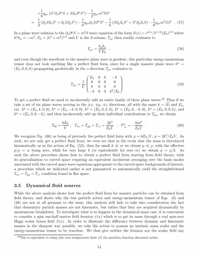
and even though the wavefront to the massive plane wave is geodesic, this particular energy-momentumtensor does not look anything like a perfect fluid form, since for a single massive plane wave kµ =(Ek, 0, 0, k) propagating geodetically in the z-direction Tµν evaluates to

Tµν =1

V

Ek 0 0 −k0 0 0 00 0 0 0−k 0 0 k2/Ek

. (59)

To get a perfect fluid we need to incoherently add an entire family of these plane waves.19 Thus if wetake a set of six plane waves moving in the ±x, ±y, ±z directions, all with the same k = |~k| and Ek,viz. kµ = (Ek, k, 0, 0), kµ = (Ek,−k, 0, 0), kµ = (Ek, 0, k, 0), kµ = (Ek, 0,−k, 0), kµ = (Ek, 0, 0, k), andkµ = (Ek, 0, 0,−k), and then incoherently add up their individual contributions to Tµν , we obtain

T00 =6EkV

, Txx = Tyy = Tzz =2k2

EkV, T µµ = −

6m2

EkV. (60)

We recognize Eq. (60) as being of precisely the perfect fluid form with ρ = 6Ek/V , p = 2k2/EkV . Assuch, we not only get a perfect fluid form, we even see that in the event that the mass is introducedkinematically as in the action of Eq. (53), then for small k ≪ m we obtain p ≪ ρ, with the effectivep/ρ = w being zero, while for very large k (or equivalently for zero m) we obtain p = ρ/3. Assuch the above procedure shows how to obtain a perfect fluid form starting from field theory, withits generalization to curved space requiring an equivalent incoherent averaging over the basis modesassociated with the curved space wave equations appropriate to the curved space backgrounds of interest,a procedure which we indicated earlier is not guaranteed to automatically yield the straightforwardTxx = Tyy = Tzz condition found in flat space.

3.5 Dynamical fluid sources

While the above analysis shows how the perfect fluid form for massive particles can be obtained fromfield theory, and shows why the test particle action and energy-momentum tensor of Eqs. (6) and(26) are not at all germane to the issue, this analysis still fails to take into consideration the factthat elementary particle masses are not kinematic, but rather that they are acquired dynamically byspontaneous breakdown. To investigate what is to happen in the dynamical mass case, it is convenientto consider a spin one-half matter field fermion ψ(x) which is to get its mass through a real spin-zeroHiggs scalar boson field S(x). In order to illustrate the difference between dynamic and kinematicmasses in the sharpest way possible, we take the action to possess no intrinsic mass scales and theenergy-momentum tensor to be traceless. We thus give neither the fermion nor the scalar field any

19This is equivalent to using (the zero temperature limit of) the partition function discussed earlier.

14

kinematic mass at all, and in order to secure the tracelessness of the energy-momentum tensor couplethe scalar field conformally to gravity, to thus yield as curved space matter action20

IM = −∫

d4x(−g)1/2[

1

2S ;µS;µ −

1

12S2Rµ

µ + λS4 + iψγµ(x)[∂µ + Γµ(x)]ψ − hSψψ]

(61)

where h and λ are dimensionless coupling constants.21 Variation of this action with respect to ψ(x) andS(x) yields the equations of motion

iγµ(x)[∂µ + Γµ(x)]ψ − hSψ = 0 , (62)

and

S ;µ;µ +

1

6SRµ

µ − 4λS3 + hψψ = 0 , (63)

while variation with respect to the metric yields (without use of any equation of motion) an energy-momentum tensor of the form

Tµν = iψγµ(x)[∂ν + Γν(x)]ψ +2

3S;µS;ν −

1

6gµνS

;αS;α −1

3SS;µ;ν +

1

3gµνSS

;α;α

−1

6S2(

Rµν −1

2gµνR

αα

)

− gµν[

λS4 + iψγα(x)[∂α + Γα(x)]ψ − hSψψ]

, (64)

with use of the matter field equations of motion then permitting us to rewrite Tµν as

Tµν = iψγµ(x)[∂ν + Γν(x)]ψ +2

3S;µS;ν −

1

6gµνS

;αS;α −1

3SS;µ;ν

+1

12gµνSS

;α;α −

1

6S2(

Rµν −1

4gµνR

αα

)

−1

4gµνhSψψ . (65)

Additional use of the matter field equations of motion then confirms that this energy-momentum tensoris indeed traceless.

In the presence of a spontaneously broken non-zero constant expectation value S0 for the scalarfield, the energy-momentum tensor is then found to simplify to

Tµν = iψγµ(x)[∂ν + Γν(x)]ψ −1

4gµνhS0ψψ −

1

6S2

0

(

Rµν −1

4gµνR

αα

)

, (66)

with flat space limit

Tµν = iψγµ∂νψ −1

4ηµνhS0ψψ . (67)

20In Eq. (61) the general-relativistic Dirac matrices γµ(x) and the fermion spin connection Γµ(x) are defined as γµ(x) =V µ

a (x)γa and Γµ = [γν(x), ∂µγν(x)]/8− [γν(x), γσ(x)]Γσµν/8 where V µ

a (x) is a vierbein and γa is a special-relativistic Dirac

gamma matrix which, with the ds2 = −(dx0)2 +(dx1)2 +(dx2)2 +(dx3)2 = ηabdxadxb metric, obeys γaγb + γbγa = −2ηab,

while ψ is given by ψ = ψ†D where D is a Hermitian flat spacetime Dirac matrix which effects DγaD−1 = γa†. In ournotation, here and throughout Hermiticity in the fermion kinetic energy sector is implicit, with iψγµ(x)[∂µ + Γµ(x)]ψ

denoting (i/2)ψγµ(x)[∂µ + Γµ(x)]ψ − (i/2)ψ[←

∂µ +Γµ(x)]γµ(x)ψ = (i/2)ψγµ(x)[∂µ + Γµ(x)]ψ + Hermitian conjugate,and iψγµ(x)[∂ν + Γν(x)]ψ denoting (i/4)ψγµ(x)[∂ν + Γν(x)]ψ + (i/4)ψγν(x)[∂µ + Γµ(x)]ψ + Hermitian conjugate inthe associated energy-momentum tensor constructed below as the symmetric Tµν = 2gµαgνβ(δIM/δgαβ)/(−g)1/2 =−(1/2)[(Vµa(x)/|V (x)|)(δIM /δV ν

a (x)) + (Vνa(x)/|V (x)|)(δIM /δV µa (x))] where |V (x)| = (−g)1/2. In this construction

we note that δgµν = VµaδVaν + δVµaV

aν , δ|V (x)| = −|V (x)|V a

µ (x)δV µa (x), and δVσc = −VµcV

aσ δV

µa , to thereby

yield (Vνa(x)/|V (x)|)(δ/δV µa (x))[

∫

d4x(−g)1/2ψγσ(x)[∂σ + Γσ(x)]ψ] = ψγν(x)[∂µ +Γµ(x)]ψ+ (1/8)ψγσ(x)([γν , γµ]);σψ−gνµψγ

σ(x)[∂σ + Γσ(x)]ψ, from which Eq. (64) then follows. (The author wishes to thank Dr. R. K. Nesbet for helpfulcomments on the material presented here.)

21As such, the action of Eq. (61) is the most general curved space matter action for the ψ(x) and S(x) fields whichis invariant under the local conformal transformation S(x) → e−α(x)S(x), ψ(x) → e−3α(x)/2ψ(x), ψ(x) → e−3α(x)/2ψ(x),gµν(x) → e2α(x)gµν(x).

15

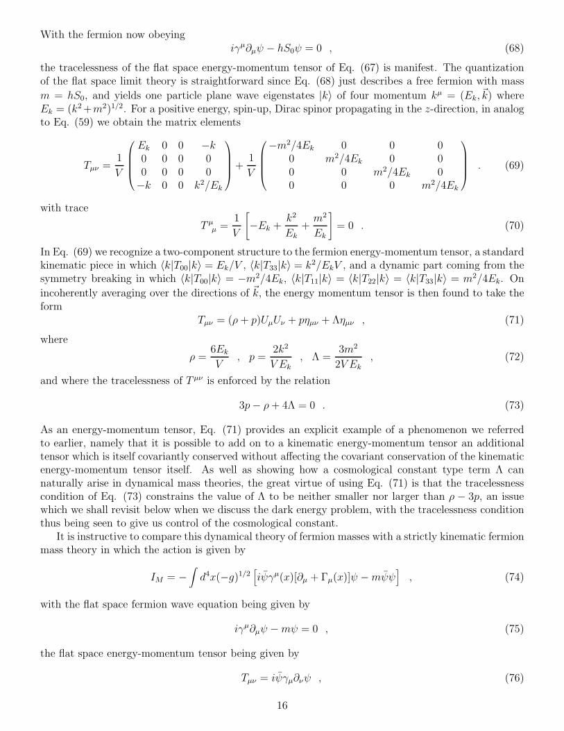
With the fermion now obeyingiγµ∂µψ − hS0ψ = 0 , (68)

the tracelessness of the flat space energy-momentum tensor of Eq. (67) is manifest. The quantizationof the flat space limit theory is straightforward since Eq. (68) just describes a free fermion with mass

m = hS0, and yields one particle plane wave eigenstates |k〉 of four momentum kµ = (Ek, ~k) whereEk = (k2 +m2)1/2. For a positive energy, spin-up, Dirac spinor propagating in the z-direction, in analogto Eq. (59) we obtain the matrix elements

Tµν =1

V

Ek 0 0 −k0 0 0 00 0 0 0−k 0 0 k2/Ek

+1

V

−m2/4Ek 0 0 00 m2/4Ek 0 00 0 m2/4Ek 00 0 0 m2/4Ek

. (69)

with trace

T µµ =1

V

[

−Ek +k2

Ek+m2

Ek

]

= 0 . (70)

In Eq. (69) we recognize a two-component structure to the fermion energy-momentum tensor, a standardkinematic piece in which 〈k|T00|k〉 = Ek/V , 〈k|T33|k〉 = k2/EkV , and a dynamic part coming from thesymmetry breaking in which 〈k|T00|k〉 = −m2/4Ek, 〈k|T11|k〉 = 〈k|T22|k〉 = 〈k|T33|k〉 = m2/4Ek. On

incoherently averaging over the directions of ~k, the energy momentum tensor is then found to take theform

Tµν = (ρ+ p)UµUν + pηµν + Ληµν , (71)

where

ρ =6EkV

, p =2k2

V Ek, Λ =

3m2

2V Ek, (72)

and where the tracelessness of T µν is enforced by the relation

3p− ρ+ 4Λ = 0 . (73)

As an energy-momentum tensor, Eq. (71) provides an explicit example of a phenomenon we referredto earlier, namely that it is possible to add on to a kinematic energy-momentum tensor an additionaltensor which is itself covariantly conserved without affecting the covariant conservation of the kinematicenergy-momentum tensor itself. As well as showing how a cosmological constant type term Λ cannaturally arise in dynamical mass theories, the great virtue of using Eq. (71) is that the tracelessnesscondition of Eq. (73) constrains the value of Λ to be neither smaller nor larger than ρ − 3p, an issuewhich we shall revisit below when we discuss the dark energy problem, with the tracelessness conditionthus being seen to give us control of the cosmological constant.

It is instructive to compare this dynamical theory of fermion masses with a strictly kinematic fermionmass theory in which the action is given by

IM = −∫

d4x(−g)1/2[

iψγµ(x)[∂µ + Γµ(x)]ψ −mψψ]

, (74)

with the flat space fermion wave equation being given by

iγµ∂µψ −mψ = 0 , (75)

the flat space energy-momentum tensor being given by

Tµν = iψγµ∂νψ , (76)

16

and the trace being given by the non-zero

T µµ = mψψ . (77)

This time, an incoherent averaging over plane wave states yields

Tµν = (ρ+ p)UµUν + pηµν , ρ =6EkV

, p =2k2

V Ek, (78)

with trace T µµ = 3p − ρ 6= 0. With both Eq. (71) and Eq. (78) leading to the covariant conservationof the kinematic (ρ + p)UµUν + pηµν , we see that both energy-momentum tensors lead to eikonalizedgeodesic motion, with the validity of the equivalence principle in no way requiring the use of Eq. (78).22

The key distinction between Eqs. (71) and (78) is that Eq. (71) contains not just the energy on thefermion field, but also that of the Higgs field that gave it its mass, an energy which couples to gravity.In dynamical theories of mass generation, gravity is thus sensitive to the Higgs field associated with thefermion, while in kinematic case it of course is not.

3.6 Implications of elementary particle physics

While it is conventional to use Eq. (78) and its analogs in current standard model cosmological studies,it is actually Eq. (71) and its analogs which is suggested by elementary particle physics. Specifically,in the standard SU(3) × SU(2) × U(1) theory of strong, electromagnetic and weak interactions, theonly mass scale present in the fundamental Lagrangian is the wrong sign, tachyonic mass term inthe Higgs potential V (S) = λS4 − µ2S2/2 with all fermions and gauge bosons getting their massesdynamically through a non-vanishing Higgs field expectation value, and all couplings between fieldsbeing dimensionless. As regards the Higgs field, it could be a fundamental field with a bona fidefundamental tachyonic mass, or it could be a dynamical manifestation of an underlying symmetrybreaking through bilinear fermion condensates, with S(x) then only being a Ginzburg-Landau typelong range order parameter (and V (S) its effective Ginzburg-Landau action) which arises when thefermion bilinear takes a non-zero expectation value in a spontaneously broken vacuum. In such a casethe underlying theory of fermions and gauge bosons would possess no intrinsic mass scales at all andwould then have a traceless energy-momentum tensor. Beyond these two possibilities for the Higgs field,inspection of the action of Eq. (61) reveals yet another origin for the wrong sign mass term, namely thatit could even arise from curvature in a theory with no fundamental mass scale at all, with Rµ

µ servingas µ2 in a non-flat background. Thus either the energy-momentum tensor of SU(3) × SU(2) × U(1) istraceless (dynamical Higgs) or its trace is given (fundamental Higgs) by the non-zero T µµ = µ2S2

0 (c.f.Eq. (56)) when S is constant. At best then the trace can only be related to the Higgs field itself, andwould thus not be given by the T µµ = 3p − ρ expected of the kinematic fluid of Eq. (78). The use ofthe perfect fluids commonly employed in standard gravity and cosmology would thus appear to be atvariance with the standard SU(3) × SU(2) × U(1) model of particle physics.23 Hence, even before we

22Analogously, if we take the scalar S(x) to be a constant in Eq. (12), Eq. (12) then reduces to Eq. (5), with testparticle motion being geodesic whether mass is kinematic or dynamic.

23In the standard particle physics model radiative corrections will lead to the generation of a trace anomaly in theorieswhose starting Lagrangian has no fundamental mass scales at all. However, such anomalies while then making the traceof the renormalized energy-momentum tensor non-zero, do not themselves introduce any new mass scale (the dimensionfour trace is proportional to terms which are quadratic in the curvature tensor) and would not in any way make the traceequal to the kinematic 3p−ρ required of Eq. (78). Moreover, it is possible to actually cancel the trace anomaly altogether,by a judicious choice of fields, a judicious choice of geometric background, or by a renormalization group fixed point atwhich the coefficient of the trace anomaly is then zero. That the trace anomaly is to be cancelled would appear to bepart of the standard cosmological wisdom anyway, since no such anomaly term contribution is ever included alongsidethe kinematic ordinary matter, kinematic dark matter and dark energy components which make up the energy contentof the standard cosmological model, and so we shall not consider the trace anomaly any further here.

17

enter into the issue of the fact that the use of standard gravity in astrophysics and cosmology leads tothe dark matter and dark energy problems, we see that the very use of such dark matter and dark energysources at all in the kinematic way in which they are commonly used is already not in accord with thestandard model of particle physics. With this word of caution in mind we shall now discuss the statusof standard gravity with its conventional kinematic perfect fluid sources, and in looking for departuresfrom standard gravity then allow for theories in which the exact energy-momentum tensor is traceless.Since the use of a traceless energy-momentum tensor in the Einstein equations of Eq. (1) would lead toa Ricci scalar which would have to vanish in every conceivable situation (to rapidly then bring standardgravity into conflict with data), when we do consider the source of gravity on the right-hand side of thegravitational equations of motion to be traceless, we will have to modify the left-hand side as well ina way which would make it automatically traceless as well. As we shall see, such a departure from thestandard theory will readily allow us to resolve both the dark matter and the dark energy problems.Having now explored constraints on the right-hand side of Eq. (1) in some detail, we turn next to anexploration of its left-hand side, and begin first with the Newtonian gravity which was its antecedent.

4 Newtonian gravity

4.1 The Newtonian potential

The Newtonian prescription for determining the non-relativistic potential φ(~r) at any point ~r due to aset of static, mass sources, mi, at points ~ri is to sum over them according to

φ(~r) = −N∑

i

miG

|~r − ~ri|(79)

where G is Newton’s constant, with the motions of material test particles then being determined via

d2~r

dt2= −~∇φ . (80)

As such, Eq. (79) contains the full content of Newton’s law of gravity, and for any given set of gravi-tational sources, any candidate theory of gravity needs to recover the associated φ(~r) in any kinematicregion in which Eq. (79) has been confirmed, to the level of precision required by available data. Todetermine what are the appropriate kinematic regions requires first testing Newtonian predictions in acandidate region using sources which are already known and prescribed in advance of data, and aftersuccess has been achieved, and only after, is one then free to use the law again in that same region toinfer the existence of other, previously unknown, sources. At the present time one can say that in thisway Newton’s law of gravity has been well-established on distance scales from the order of millimeters(the smallest distance scale on which there has been testing) out to distances of the order of 1015 cmor so (viz. solar system distance scales). At much larger distances all tests which use only the sourceswhich were known in advance of observation have been found to fail, with additional (dark matter)sources always having to be invoked after the fact, with the validity of Newton’s law yet to be con-firmed on those distances.24 The establishing of a given law in one kinematic region cannot be regardedas evidence for its validity in others.

As regards solar system tests of Newton’s law of gravity, these tests are spectacular, with theplanets being found to move according to Eq. (80) to very high accuracy when the sun and the planets

24Testing the validity of Newton’s law on a distance scale such as galactic would require knowing the dark matterdistribution in a galaxy in advance of measurement of the orbital velocities of the material in it.

18

themselves are taken to be the sources. To a very good approximation the planets move around thesun with a centripetal acceleration of the form

v2

r=GM⊙

r2, (81)

and have Keplerian fall-off of velocity with distance of the form

v =G1/2M

1/2⊙

r1/2(82)

where M⊙ is the mass of the sun. In fact so reliable was this law found to be in the solar system whenonly known visible sources were used, that when the orbit of Uranus was found to depart slightly fromthe Newtonian expectation, a perturbation due to a then undetected nearby planet was proposed, withthe subsequent detection of Neptune giving dramatic confirmation of Newton’s law of gravity at thatdistance scale.

While Newton’s law had always been thought to hold on all solar and sub-solar distance scales,recently it has come in to question on very small laboratory scales of order millimeters or so. While themeter or so distance region had actually been quite throughly searched (though to no avail) when it wasthought that there might be a so-called fifth force operative on those distance scales (fifth since it wouldbe in addition to the strong, electromagnetic, weak and gravitational forces), recent studies of largeextra dimension physics had led to a reopening of the issue with a focus on the even smaller millimeterregion distance scale. While there has been a longstanding theoretical interest in the possible existenceof additional spacetime dimensions beyond the four established ones, it had generally been presupposedthat such dimensions would be truly microscopic, possibly being as small as the 10−33 cm Planck length.In an attempt to resolve the longstanding hierarchy problem of understanding why there was such ahuge disparity between the MEW = 103 GeV electroweak and the MPL = 1019 GeV gravitational massscales, Arkani-Hamed, Dimopoulos and Dvali [7] found a candidate extra dimension based solution inwhich rather than be microscopic, the additional dimensions beyond four would instead need to be of theorder of millimeters. In such a situation gravitational flux lines could then spread out to such distancesin the extra dimensions, and therefore lead to modifications to standard gravity at the millimeter level.Following on the work of Arkani-Hamed, Dimopoulos and Dvali, Randall and Sundrum [8, 9] found analternate way to address the hierarchy problem which required the geometry in the extra dimensionsnot to be the Minkowski one that had always been assumed in higher dimensional theories, but ratherto be anti-de Sitter. In such a situation the extra dimensions could then not only be large but eveninfinite in size, with the curvature of the anti-de Sitter space acting as a sort of refractive mediumwhich would sharply inhibit the penetration of gravitational flux lines into the higher dimensions. Insuch theories there could again be departures from Newton’s law at the millimeter level, which thusprompted a renewed search for possible millimeter region departures. Since for the moment, none hasyet actually been detected [10], the issue should be regarded as open, and so we shall assume herethe validity of Eq. (79) on all solar and sub-solar distance scales including millimeter ones and below,with the deriving of the Newtonian phenomenology on such scales thus being set as a requisite for anycandidate gravitational theory.

4.2 The second order and fourth order Poisson equations

While Eq. (79) contains the full content of Newton’s law of gravity, in order to actually perform theneeded sum over sources, it very convenient to recast Newton’s law in the form of a second order Poissonequation. Thus if we set

∇2φ(~r) = g(~r) , (83)

19

we can write the potential as

φ(~r) = −1

4π

∫

d3~r′g(~r′)

|~r − ~r′|, (84)

with the potential exterior and interior to a spherically symmetric static source of radius R then beinggiven by

φ(r > R) = −1

r

∫ R

0dr′r′2g(r′) , φ(r < R) = −

1

r

∫ r

0dr′r′2g(r′) −

∫ R

rdr′r′g(r′) . (85)

However, Eq. (83) is not the only Poisson type equation which will lead to a 1/r potential. Thus if wefor instance consider the fourth order

∇4φ(~r) = h(~r) , (86)

we can write the potential as

φ(~r) = −1

8π

∫

d3~r′h(~r′)|~r − ~r′| , (87)

with the potential exterior and interior to a spherically symmetric static source of radius R then beinggiven by

φ(r > R) = −r

2

∫ R

0dr′r′2h(r′) −

1

6r

∫ R

0dr′r′4h(r′) ,

φ(r < R) = −r

2

∫ r

0dr′r′2h(r′) −

1

6r

∫ r

0dr′r′4h(r′) −

1

2

∫ R

rdr′r′3h(r′) −

r2

6

∫ R

rdr′r′h(r′) . (88)

Moreover, recovering a 1/r potential is not even restricted to the above choices of Poisson equation,since the sixth order ∇6φ(~r) = k(~r) would yield an exterior potential of the generic form φ ∼ 1/r+r+r3,with the pattern repeating for all higher even number of derivative Poisson equations. Characteristic ofall of these possible Poisson equations is the fact that we recover a 1/r term for each and every one ofthem, and in all of them the terms which depart from a pure 1/r form are all only important at largerdistances (viz. just the distances on which the dark matter problem is encountered), with there beingno modifications to the 1/r law at very small distances. Providing that the r, r3 and so on type termsare all negligible on solar system distance scales, all of these Poisson equations will thus reproduce thestandard Newtonian solar system phenomenology.

Now at first glance the expressions for the coefficients of the 1/r terms in Eqs. (85) and (88) appearto differ since they are given as different moments of the source. However, this is not of concern sincemeasurements of φ(r) in the r > R region where there are data can never uncover any informationregarding the behavior of the integrand in Eq. (85) in the r < R region. What is required of the 1/rterm in the r > R region is only that it conform with the large r behavior required by the originalNewton law of Eq. (79) (and thus the all r > R behavior since 1/r is the unique behavior of the Newtonterm in the entire exterior region), viz. that for a set of sources all with the same mass m the potentialbehave as

φ(r > R) = −NmG

r, (89)

i.e. that the coefficient of the 1/r term be linear in the number of sources N . To achieve such a linearityin the second order Poisson equation case one can choose to set

g(r < R) = mGN∑

i=1

δ(r − ri)

r2(90)

in the r < R region, though as we had just noted, this is not mandated by Eq. (79). (While use of thisparticular g(r < R) is sufficient to give Eq. (89), it is not necessary.) What is necessary is only that

20

there be N discrete sources, with Eq. (79) only counting the number of them in the r > R region. Toachieve exactly the same result through the use of the fourth order Eq. (88), it is convenient, thoughnot mandatory, to consider as source25

h(r < R) = −γc2N∑

i=1

δ(r − ri)

r2−

3βc2

2

N∑

i=1

[

∇2 −r2

12∇4

] [

δ(r − ri)

r2

]

, (91)

with its insertion in Eq. (88) yielding

φ(r > R) = −Nβc2

r+Nγc2r

2. (92)

As we see, the coefficient of the 1/r term is again linear in the number of sources, with Newton’s law ofgravity only counting the number of discrete sources that are present in the r < R region. ComparingEqs. (89) and (92), we see that we can once and for all define β = mG/c2 at the individual discretesource level (a level which could be microscopic), without ever needing to decompose βc2 into separatem and G pieces, with only the Schwarzschild radius of the source (viz. 2mG/c2 in the second ordercase and 2β in the fourth order) ever being measurable gravitationally.26

It is important to stress that it is the presence of two independent singularities in the source of Eq.(91) which leads to the logical independence of the β and γ coefficients, since if we could approximatethe source h(r) by a constant source h(r) = h, we would instead have to conclude that the coefficientsof the two potential terms would be related according to

φ(r > R) = −NhR5

30r−NhR3r

6, (93)

and thus have a ratio of order the radius squared of the source. This is to be contrasted with the choiceof a constant source g(r) = g in the second order case where the potential is then given by

φ(r > R) = −NgR3

3r. (94)

Since a comparison of Eqs. (89) and (94) would entail that one can make the identification mG = gR3/3,a view of gravitational sources has developed that macroscopic gravitational sources can be treated asbeing continuous rather as being a collection of independent discrete microscopic sources. However,apart from not at all being mandated by the successful use of Eq. (89), the issue is in fact not evenaddressable if one only makes measurements in the exterior r > R region. However, in the fourth orderPoisson case the issue does become relevant, because here one does measure more than just one momentof the source, with the higher derivative theory thus being able to probe deeper into the source. Thuswithin the fourth order theory, an experimental determination of the ratio of the coefficients of the 1/rand r terms which would indicate that the ratio of the two coefficients is very far from being of order thesquare of the radius of a given macroscopic source, would indicate that the macroscopic source would

25We choose the particular [∇2− (r2/12)∇4](δ(r−ri)/r2) source rather than the more straightforward ∇2(δ(r−ri)/r

2)one, since unlike the latter, the former one happens to be positive definite. An additional virtue of this particular choice ofsource is that it only couples to the fourth moment integral and not to the second moment one; and with the δ(r− ri)/r

2

source only coupling to the second moment integral and not to the fourth moment one, the logical independence of thetwo moments is thus established.

26Even if the microscopic βc2 were not to be equal to the product of the conventionally defined m and G (not that weknow what the gravitational coupling of a microscopic source is), the use of the coefficient Nβc2 would then lead to aestimate for the number of atoms in a macroscopic source such as the sun which would be different from the conventionalone, a point which is not of concern since without appealing to the mG coefficient, we do not know how many atoms thereanyway are in the sun, with the standard estimate of the number being based on the a priori use of the mG coefficient.

21

have to be composed of microscopic components which are discrete. Quite remarkably then, higherorder derivative theories open up the possibility of establishing discreteness at the microscopic levelfrom macroscopic measurements alone.27 Moreover, below we shall actually apply the potential of Eq.(92) to galactic rotation curves, to find that the β∗ and γ∗ coefficients of the fourth order theory stellarpotential

φ∗(r > R) = −β∗c2

r+γ∗c2r

2(95)

actually are very far from possessing a ratio β∗/γ∗ which is anything like the square of a typical stellarradius (numerically we find (β∗/γ∗)1/2 ∼ 1023 cm, with the γ∗c2r/2 term first becoming competitivewith the β∗c2/r term on galactic distance scales). Within the framework of a gravity which is based onfourth order equations then we can conclude that matter must be discrete at the microscopic level.

While the second order Poisson equation of Eq. (83) does yield the Newtonian potential of Eq. (89)as solution, there is actually a critical difference between the use of the second order Newton potentialand Poisson equation on the one hand and the use of their fourth order counterparts given as thepotential of Eq. (92) and the Poisson equation of Eq. (86) on the other. Specifically, while the fourthorder potential of Eq. (92) does nicely reduce to the second order potential of Eq. (89) in the smallr limit, the fourth order Poisson equation itself never reduces to the second order one in any limit atall. It is thus possible for solutions to two different equations to approximate each other very closelyin some kinematic region even while the equations to which they are solutions never approximate eachother at all. The equations which describe any candidate alternate theory of gravity thus do not atall need to reduce to those which describe the standard theory. Rather, it is only the solutions to thealternate theory which have to recover the solutions to the standard theory in any of the kinematicregions in which the standard theory solutions have themselves been tested.28 Outside of such regionsthe alternate theory can then provide for departures from the standard theory expectations, somethingwe will capitalize on below to explain galactic rotation curve systematics without the need to invokedark matter. The essential difference between the second order Poisson equation and the fourth orderone, is that once the second order Poisson equation is specified as being the fundamental equation ofmotion, there is no possibility to ever get any departure from Newton’s law on any distance scale atall, something which is allowed for in a higher order theory. Since the Einstein equations of Eq. (1)were explicitly constructed so that their non-relativistic weak gravity limit would be the second orderPoisson equation, the Einstein equations thus lock non-relativistic weak gravity into being Newtonianon all distance scales, and to thus be so even on distances well beyond the solar system ones whereNewton’s law of gravity was originally established. In this sense then the dark matter problem couldoriginate in the lack of reliability of the extrapolation of standard solar system wisdom to altogetherlarger distance scales.

4.3 Universal acceleration scale and the MOND theory

While the above discussion has focused on the standard Newtonian picture and those allowed departuresfrom it which are associated with a critical distance scale, an alternate form of allowed departure hasbeen suggested by Milgrom [11, 12, 13], one which has proven to be remarkably instructive and fruitful.Specifically, on noting that the centripetal accelerations of particles in orbits around galaxies were

27As a historical aside, we note that since the use of higher order gravity can thus provide for a macroscopic manifestationof the existence of atoms, it thus meets an objective which was first sought by Boltzmann, one which was part of hismotivation for developing kinetic theory (and which was subsequently achieved by a determination of a finite value forAvogadro’s number by macroscopic means).

28If the alternate equations of motion did reduce to the standard ones in some limit, then of course so would theirsolutions. However, the converse is not true, since the alternate theory solutions are still able to reduce to the standardtheory solutions even if there is no such parallel for the equations of motion themselves.

22

typically much smaller than those associated with the orbits of planets around the sun or satellitesaround the earth, Milgrom suggested that the determining factor was not in fact a distance scale atall but rather an acceleration one, with departures from the standard wisdom occurring wheneveraccelerations of particles dropped below some critical universal acceleration scale a0. Quite remarkably,Milgrom found that it is actually possible to choose such an a0 so that its effects would be of significancefor galaxies and yet leave solar system phenomenology untouched.29 In contrast to proposals which seekto modify the right-hand side (viz. the gravitational side) of Eq. (80), Milgrom instead proposed tomodify the left-hand side (viz. the inertial side) with the proposal thus being known as MOND (modifiedNewtonian dynamics). Specifically Milgrom replaced Eq. (80) by

µ(

a

a0

)

~a = ~f (96)

where ~a = d2~r/dt2 is the ordinary acceleration, ~f = −~∇φ is the gravitational force and µ(a/a0) is themodification. In order for this modification to reduce to the standard Newton law when a ≫ a0, thefunction µ(x) has to behave as µ(x≫ 1) → 1. Guided by the fact that many prominent spiral galaxiespossess rotational velocity curves which are flat (i.e. the rotational velocity v is independent of thedistance R from the center of the galaxy), and that the velocities of these particular galaxies obey theempirical Tully-Fisher law which relates v to the total luminosity L of the galaxy as v4 ∼ L, Milgromfurther suggested that at very small x the function µ(x) should behave as µ(x ≪ 1) → x, since thecentripetal accelerations a = v2/R ≪ a0 of orbits in a galaxy of mass M would then obey

a2

a0

=v4

a0R2=MG

R2, (97)

and thus yield the R independent v4 = a0MG. Then, if the mass involved was just the luminous massof the galaxy, it would be related to the luminosity of the galaxy by M = (M/L)L where M/L is themass to light ratio of the galaxy, with both the flatness of galactic rotation curves and the Tully-Fisherrelation thereby being obtained from luminous matter alone.

As a proposal, the relation of Eq. (96) is perhaps a little bit too strong a departure from the standardpicture, since as such it would modify the inertial side of Newton’s second law of motion not just forgravitational processes but for non-gravitational ones as well, processes for which there are no knownproblems. Additionally, since the proposal is a modification of the inertial side of Newton’s second lawof motion, in an accelerating coordinate system Eq. (96) would not readily recover Eqs. (4) and (5). Toget a sense of what might instead happen, one possible way to effect a covariant generalization of Eq.(96) is to replace the acceleration ~a by the contravariant D2xλ/Dτ 2 of Eqs. (4) and (5), to introduce afour-vector V λ which reduces to V λ = (1, 0, 0, 0) in a non-accelerating coordinate system, and to takeµ(x) to be a general coordinate scalar function of

x =Vλa0

D2xλ

Dτ 2(98)

where the parameter a0 is then a general coordinate scalar with the dimensions of acceleration. Whilethe presence of such a Vλ would lead to frame-dependent effects, such departures from standard wisdomneed not necessarily be in conflict with observation if µ(x) is sensibly close to one in the kinematicregime where tests of the equivalence principle and preferred frame effects have so far been made.

Nonetheless, since it would be more economical not to have to make so radical a conceptual departurefrom standard wisdom, an alternative procedure for introducing a universal acceleration a0 would be

29Phenomenologically a0 was found to be of order 10−8 cm/sec2, to be compared with an acceleration at the outerlimits of the solar system of order 10−3 cm/sec2 due to the pull of the sun.

23

to have it instead appear on the gravitational side of Eq. (80), with Eq. (80) then being replaced by

~a = ν

(

f

a0

)

~f (99)

instead. To get a sense of what the function ν(y) might look like, we consider a particularly simplechoice for µ(x) which meets its required large and small x limits, viz.

µ(x) =x

(1 + x2)1/2, (100)

to then find that ν(y) and ~a are given by

ν(y) =

(

1

2+

(y2 + 4)1/2

2y

)1/2

(101)

~a =

(

1

2+

(f 2 + 4a20)

1/2

2f

)1/2

~f . (102)

With the two relevant limits of the function ν(y) being ν(y ≫ 1) → 1, ν(y ≪ 1) → 1/y1/2, we thusrecover Eq. (80) when f ≫ a0, and come right back to Eq. (97) when f ≪ a0, with Eqs. (96) and(99) leading to the same gravitational phenomenology. Having now presented an analysis of Newtoniangravity and some possible allowed departures from it, we turn next to a discussion of Einstein gravity.

5 Einstein gravity

5.1 Einstein gravity for static sources and the Newtonian limit

In his construction of a covariant theory of gravity, even though Einstein used a fundamental principle,viz. the equivalence principle, to identify the metric gµν as the gravitational field, his choice for thedynamical equation of motion which was to then fix the metric, viz. Eq. (1), appears to have been basedon a phenomenological consideration, namely that the theory recover the standard second order Poissonequation in the non-relativistic, weak gravity limit. As such, the second order Einstein equations can beviewed as being a covariant generalization of the second order Poisson equation of Eq. (83), replacingit by ten equations (reducible to six by gauge invariance) of which only the (00) component equationwould be of order one in the standard non-relativistic, weak gravity limit in which the components ofTµν other than T00 are taken to be negligible compared to T00 itself. The great virtue of the Einsteinequations is that in prescribing a covariant generalization of the second order Poisson equation, it notonly incorporated Newtonian gravity, but also provided it with general relativistic corrections whichcould then be tested, leading to the three classic tests of general relativity, the gravitational red shift,gravitational bending of light, and the precession of planetary orbits. With the Einstein equations notonly satisfying these three tests, but doing so in truly spectacular fashion, by and large the consensusin the community is that the issue is therefore considered settled, with the Einstein equations being thetrue equations of gravity which no longer need to be open to question.

However, it is important to note that while Einstein’s original construction was motivated by thesecond order Poisson equation, the application of Eq. (1) to the three classic solar system tests is notactually sensitive to this particular aspect of the Einstein equations at all. Specifically, what is neededfor the three tests is only knowledge of the metric exterior to a static, spherically symmetric source, viz.the Schwarzschild metric as given earlier as Eqs. (41) and (50), a metric which obeys Rµν = 0 in thesource-free region. As such, the exterior Schwarzschild solution is parameterized by a parameter MG

24

associated with a given source, and while this parameter can be determined from a matching of theexterior solution of Eq. (50) to the interior solution of Eq. (47) to yield Eq. (51), no use of Eq. (51) isactually made in the analysis of the classic tests. While the Rµν = 0 condition does indeed follow fromEq. (1) in the source-free Tµν = 0 region, Eq. (1) does not follow from this fact, i.e. knowing that Rµν

vanishes in the source-free region is not sufficient to determine what Rµν is to be equal to in regionswhere it does not vanish. To emphasize the point, we note that while functional variation of the secondorder Einstein-Hilbert action

IEH = −c3

16πG

∫

d4x(−g)1/2Rαα (103)

with respect to the metric yields the Einstein tensor according to

16πG

c3(−g)1/2

δIEHδgµν

= Gµν = Rµν −1

2gµνRα

α , (104)

variation of the fourth order general coordinate scalar actions

IW1=∫

d4x(−g)1/2[Rαα]

2 (105)

andIW2

=∫

d4x(−g)1/2RαβRαβ (106)

respectively yield [14]

1

(−g)1/2

δIW1

δgµν= W µν

(1) = 2gµν(Rαα)

;β;β − 2(Rα

α);µ;ν − 2Rα

αRµν +

1

2gµν(Rα

α)2 , (107)

and

1

(−g)1/2

δIW2

δgµν= W µν

(2) =1

2gµν(Rα

α);β

;β +Rµν;β;β − Rµβ;ν

;β −Rνβ;µ;β − 2RµβRν

β +1

2gµνRαβR

αβ . (108)

Then, since the Schwarzschild solution is one in which the Ricci tensor vanishes, in the Schwarzschildsolution it follows that covariant derivatives of the Ricci tensor vanish as well, with both W µν

(1) and

W µν(2) thus vanishing when Rµν = 0. Moreover, this same argument immediately generalizes to general

coordinate scalar actions based on even higher powers of the Ricci scalar or Ricci tensor. The exteriorSchwarzschild solution is thus an exterior solution to any pure metric theory of gravity which uses anyRicci tensor based higher order action in place of the Einstein-Hilbert action,30 with all of them thussatisfying the three classic tests.31 Thus, in complete parallel to our earlier discussion of the differencebetween the second and higher order Poisson equations, we see that even though there is no limit inwhich any linear combination of W µν

(1) and W µν(2) reduces to the Einstein tensor of Eq. (104), nonetheless

the use of any such combination as a gravitational tensor which could replace Gµν in Eq. (1) wouldstill lead to the Schwarzschild solution. The Schwarzschild solution thus bears the same relation to theEinstein-Hilbert action and its higher order generalizations as the Newton potential does to the Poissonequation and its higher order generalizations, with use of the Einstein equations only being sufficient tosecure the three classic tests but not at all necessary. Hence, as had first been noted by Eddington aslong ago as only shortly after he himself led an expedition in 1919 to confirm that light did indeed bend

30This would not necessarily be true for any higher order Riemann tensor based action since the Schwarzschild metricis not Riemann flat, only Ricci flat.

31While the vanishing of the Ricci tensor implies the vanishing of its derivatives as well, the vanishing of the derivativescan be achieved without the Ricci tensor itself needing to vanish, with the vanishing of tensors such as Wµν

(1) or Wµν(2) thus

being achievable by additional, non-Schwarzschild type solutions as well, a point we shall return to below.

25

as it passed by the sun, the success of the three classic tests does not secure the validity of the Einsteinequations, with other options being possible. Indeed, at that time Eddington issued a challenge to thecommunity to tell him which gravitational action then was the correct one to use, a challenge that thecommunity has never answered even though it goes directly to the heart of gravitational theory.

Beyond the three classic tests of general relativity, the only other test on solar system sized distancescales is the decay of the orbit of a binary pulsar, an effect which again only involves an exterior metric,this one due to the presence of two stellar sources rather than just the one involved in the solar systemtests. The decay of the orbit is due to gravitational radiation reaction, with each star in the binaryresponding to retarded gravitational signals emitted by the other and not to instantaneous ones. Suchretardation effects will exist in any covariant metric theory of gravity since in all of them gravitationalinformation cannot be communicated faster than the speed of light, and in all of them there will thusbe some decay of the binary pulsar orbit. While there thus will be orbit decay not only in Einstein-Hilbert based gravity but also in its higher order alternatives, nonetheless all such alternatives facethe (calculationally daunting) challenge of actually obtaining the specific amount of decay which hasactually been observed, with calculations having so far only been carried through (and with stunningsuccess) is the second order Einstein theory itself.

5.2 The Einstein static universe and the cosmological constant

The one situation in which the full content of the Einstein equations is felt is in cosmology, since in thatcase both sides of Eq. (1) are non-zero, with cosmological observations being made inside the universeand thus in the region where Tµν is explicitly non-zero. In order to prepare for the discussion of the darkenergy problem and the accelerating universe to be given below, it is useful to recall Einstein’s effort toproduce a static universe solution to the Einstein equations through the introduction of a cosmologicalconstant. In order to see the structure of the Einstein model it is instructive to start not with a staticmodel but rather with the general time dependent Robertson-Walker geometry of Eq. (36) and thegeneric source of Eq. (37) with its two separate time-dependent functions C(t) and D(t). For such aset-up the Einstein equations of Eq. (1) yield

3cR = −4πG(C + 3D)R (109)

and

R2 + kc2 =8πG

3cCR2 . (110)

A solution in which C, D and R are all constant is then obtained when

D

C= −

1

3, k =

8πG

3c3CR2 . (111)

On taking C to be positive, we see that k would need to be positive too (viz. topologically closed3-space), while D would have to be negative, with the Einstein static universe thus being supportableby a source with D/C = −1/3. Fluids in which D/C is negative are known as quintessence fluidsand have recently come into prominence [15] through the discovery of the accelerating universe, witha quintessence fluid with C + 3D < 0 then leading to a net cosmic acceleration (R > 0) in Eq. (109),though its role in the Einstein model is to put the acceleration precisely at the R = 0 borderline where itit is neither positive nor negative. In his actual construction, Einstein himself did not use the languageof quintessence fluids. Rather, Einstein used an energy-momentum tensor containing just an ordinarynon-relativistic matter fluid with a density ρm and zero pressure pm, and actually modified Eq. (1) byadding a cosmological constant term to its left-hand side according to

−c3

8πG

(

Rµν −1

2gµνRα

α

)

+ Λgµν = T µν . (112)

26

With the cosmological constant term itself having the form of a perfect Robertson-Walker geometryfluid with energy density ρΛ = cΛ > 0 and pressure pΛ = −cΛ < 0 (so that the cosmological constantterm itself can be thought of as being a quintessence fluid with pΛ = −ρΛ and ρΛ + 3pΛ < 0), we canrelate ρm and Λ to C and D according to C = ρm/c+Λ, D = −Λ. The requirement that C and D obeyC + 3D = 0 then requires that ρm and Λ be related according to the very specific fine-tuned relation

2cΛ = ρm . (113)

Since on its own the ordinary ρm fluid would lead to R < 0 in Eq. (109) while on its own a positivecosmological constant would lead to R > 0, as we thus see, to get the Einstein model to be static weneed to fine-tune the attraction generated by the energy density ρm and the repulsion generated by thecosmological constant Λ so that they precisely cancel each other. Interestingly, we shall encounter areflection of such a fine-tuning below in our discussion of the dark energy problem.

With Slipher and Hubble’s discovery of the expansion of the universe Einstein realized that therewas no further need for a static cosmology,32 and so he abandoned the cosmological constant. However,with the recent discovery of the acceleration of the universe (i.e. not just an expanding R > 0, butalso an accelerating R > 0), the cosmological constant has come back into prominence, not just as afundamental term of the form inserted on the left-hand side of Eq. (112) but also as a dynamicallygenerated spontaneous symmetry breakdown contribution to the energy-momentum tensor on the right-hand side of Eq. (112), with current cosmology requiring these two types of cosmological constant tocancel each other to unbelievable precision.

From a theoretical perspective, the very fact that one is able to introduce the Λgµν term on theleft-hand side of Eq. (112) at all is a reflection of the fact that Einstein’s very choice of the originalEq. (1) did not derive from a fundamental principle but only from the phenomenological need torecover Newton’s law.33 Indeed, it was phenomenology which lead him first to introduce and thensubsequently to remove the cosmological constant term. It is this lack of a principle which renders thechoice of gravitational action non-unique, with there then being no principle with which to control thecontribution of the cosmological constant. In addition, the use of Eq. (1) dictates that the low energylimit of the theory is the second order Poisson equation not just on solar system distances but on alldistances. And so we turn now to a study of the motions of particles on larger distance scales to seejust how well the second order Poisson equation and its Newtonian potential solution then fare.

6 The dark matter problem

6.1 The galactic rotation curve problem

It is really quite remarkable how early in the study of galaxies and then clusters of galaxies that massdiscrepancies started to appear. Specifically, not all that long after Shapley’s work on the shape andsize of the Milky Way galaxy and Hubble’s demonstration that the spiral nebulae were distant galaxiesin their own right, Oort’s measurements [16] of the velocities of stars in our local solar neighborhoodand Zwicky’s [17] and then Smith’s [18] measurements of the velocity dispersions of galaxies in clustersof galaxies all pointed to discrepancies. Since the discrepancy that Zwicky detected was based on theuse of the Newtonian gravity virial theorem, Zwicky was able to conclude that unless the virial theoremitself did not hold for clusters (either because Newton’s law did not hold on those distances or becausethe cluster had not yet virialized), there then had to be more mass in the cluster than he could detect.As such, it was thought at the time that any such missing mass would be in the form of astrophysical

32Even in his model, any departure from the 2cΛ = ρm fine-tuning condition would lead to a non-static cosmology.33Phenomenological that is unless there is some as yet unknown principle which would actually require the validity of

Newton’s law on all distance scales, since for the moment Newton’s law itself is only phenomenological.

27

objects which were too faint to be detectable, with the notion that the missing matter might be of anentirely different form that could never be detected optically at all coming only altogether later whenit was realized that modern elementary particle physics could actually provide such so called Wimp(weakly interacting massive particle) objects.

While there continued to be further indications of mass discrepancies over time (for a history seee.g. [19]), the situation started to become critical following the HI 21 cm radio studies of the spiralgalaxies NGC 300 and M33 by Freeman [20] and of M31 by Roberts and Whitehurst [21] which foundno sign of the expected Keplerian fall-off of rotational velocity v with distance R from the center of thegalaxy. With hydrogen gas being distributed in spiral galaxies out to much further distances than thestars themselves, the HI studies were thus the ideal way to probe the outer reaches of spiral galaxies,and thus the ideal probe to test for the Keplerian fall-off expected of the rotation velocities of particleswhich were located far beyond the visible stars (viz. the visible mass) of the galaxies. Moreover, themeasurement of such rotation velocities would be unhindered by projection effects if studies were madeof spirals that were close to being edge on along our line of sight.

The continuing persistence of the cluster problem and concern in general about mass discrepanciesprompted detailed exploration of outer region galactic rotation curves, with early systematic surveysbeing made by Bosma [22] and Begeman [23] as part of the University of Groningen Westerbork SynthesisRadio Telescope survey. What was found in these and in many related studies was that the outerregion rotation velocities were systematically larger than the Keplerian expectation, with none givingany indication of a fall-off at all. In Fig. 1 we display the rotational velocity curves of a sample of elevenspiral galaxies which have been identified by Begeman, Broeils and Sanders [24] as being particularlyreliable and characteristic of the general pattern of behavior of galactic rotation curves which has beenfound, with their paper giving complete data references. With the stellar surface matter density of eachspiral galaxy in the sample behaving as

Σ(R) = Σ0e−R/R0 ,

N∗ = 2π∫ ∞

0dRRΣ(R) = 2πΣ0R

20 , (114)

where R0 is the scale length and N∗ is the total number of stars,34 in Fig. 1 we have plotted therotation velocities (in units of km/sec) in each given galaxy as a function of R as measured in unitsof that particular galaxy’s own scale length, with the rotation curves being displayed in the figure inorder of increasing luminosity from the lowest (DDO 154) to the highest (NGC 2841) in the sample. InTable 1 we provide some characteristics of the galaxies, and note that the luminosities of the galaxiesin the selected sample range over a factor of order a thousand.

To get a quick sense of what the luminous Newtonian expectation for galaxies might look like, wenote that for an infinitesimally thin disk of stars with distribution Σ(R) = Σ0e

−R/R0 and potentialV ∗(r) = −β∗c2/r = −M⊙G/r, the total centripetal acceleration is then given by [20]

v2lum

R= glum

β =N∗β∗c2R

2R30

[

I0

(

R

2R0

)

K0

(

R

2R0

)

− I1

(

R

2R0

)

K1

(

R

2R0

)]

. (115)

(In Appendix A we provide a straightforward derivation of this relation.) From the behavior of themodified Bessel functions, the v(R) velocity profile associated with Eq. (115) is found to consist of aninitial rise from R = 0 up to a peak at R = 2.2R0 which is then followed by a steady fall-off. With Σ(R)

34We assume that light traces mass, so that the surface matter density is proportional to the measured luminous surfacebrightness with a mass to light ratio which is independent of R.

28

8 0

6 0

4 0

2 0

0

1 086420

DDO170

8 0

6 0

4 0

2 0

0

76543210

NGC3109

150

100

5 0

0

1 61 41 21 086420

NGC6503

6 0

4 0

2 0

01 51 050

DDO154

8 0

6 0

4 0

2 0

0

86420

NGC1560

100

8 0

6 0

4 0

2 0

0

86420

UGC2259

200

150

100

5 0

0

1 41 21 086420

NGC3198

150

100

5 0

0

1 21 086420

NGC2403

300

200

100

0

1 086420

NGC7331

250

200

150

100

5 0

0

1 51 050

NGC2903

400

300

200

100

0

2 01 51 050

NGC2841

Figure 1: Some typical measured galactic rotation velocities (in km/sec) with their quoted errors asplotted as a function of R/R0 where R0 is each galaxy’s own optical disk scale length. The dashed(falling) curve shows the velocities that would be produced by the luminous Newtonian contributionalone. The dash-dotted (rising) curve shows the velocities that would be produced by the linear poten-tials of the alternate conformal gravity theory which is discussed below, and the full curve shows theoverall predictions of that theory, with no dark matter being assumed.

29

Table 1: Characteristics of the eleven galaxy sample

Galaxy Distance Luminosity R0 (v2/c2R)last (M/L)(Mpc) (109LB⊙

) (kpc) (10−30cm−1) (M⊙L−1B⊙

)

DDO 154 3.80 0.05 0.48 1.51 0.71DDO 170 12.01 0.16 1.28 1.63 5.36NGC 1560 3.00 0.35 1.30 2.70 2.01NGC 3109 1.70 0.81 1.55 1.98 0.01UGC 2259 9.80 1.02 1.33 3.85 3.62NGC 6503 5.94 4.80 1.73 2.14 3.00NGC 2403 3.25 7.90 2.05 3.31 1.76NGC 3198 9.36 9.00 2.72 2.67 4.78NGC 2903 6.40 15.30 2.02 4.86 3.15NGC 7331 14.90 54.00 4.48 5.51 3.03NGC 2841 9.50 20.50 2.39 7.25 8.26

typically reaching to about four scale lengths before becoming negligible, the visible stellar materialin the galaxy is thus contained almost entirely within this region (the optical disk), with Eq. (115)asymptoting to the Keplerian

v2lum

R→

N∗β∗c2

R2(116)

far outside the optical disk. To treat the luminous Newtonian contribution more accurately we needto allow for the fact that the optical disk actually has a thickness (with its own scale height z0), thatthe HI gas comes with its own surface brightness distribution and can have a total mass as high as15 per cent or so of the luminous mass, and that the two largest galaxies in the sample also have acentral bulge. Using the calculational tools presented in Appendices A, B and C the contributions ofall of these various components can readily be determined for each galaxy in the sample, with the exactluminous Newtonian expectation for v(R) reported in the typical calculation of [25] being exhibitedas the dashed curves in Fig. 1. In generating this total luminous Newtonian contribution, the totalnumber of stars N∗ in each galaxy was adjusted so that the luminous Newtonian contribution wouldaccount for the entire rotational velocity at the R = 2.2R0 peak (the maximum disk prescription), withthe obtained values for N∗ being presented in Table 1 as galactic mass to light ratios M/L which thusexpress N∗ in terms of the measured total luminosity of each galaxy. As we see, normalizing to thismaximum disk prescription then completely accounts for the entire initial rise in the rotation curve,to therefore indicate that the inner region is well described by the luminous Newtonian contributionalone. However, as we also see from Fig. 1, in the outer regions of the galaxies the luminous Newtoniancontributions totally underaccount for the measured velocities.35 This then is the mass discrepancyproblem in galaxies, and as such it is actually far more severe than the cluster problem, since it is basednot on any statistical averaging over the velocities of many galaxies in a cluster or on any assumptionregarding their virialization, but only on looking at individual orbits in galaxies one by one just as wasdone for planetary orbits in the solar system. Not only do we find such discrepancies in galaxies, wewryly note if the galactic data were the only data that were available to us and we had no solar system

35The maximal disk prescription takes the luminous Newtonian contribution to be as large as it possibly can be withoutovershooting the inner region data. Since this simultaneously fixes the normalization of the Newtonian contribution tothe outer region, it thus represents the best that the luminous Newtonian contribution can possibly do in the outer region.And even if we were to change the overall normalization of N∗, this would anyway not change the shape of the luminousNewtonian contribution, with its behavior at large R still falling off even then.

30

data at all, then from the measured galactic rotational velocities alone it would not be possible to inferan inverse square gravitational law at all.36

6.2 The dark matter solution for galaxies

Given the prior experience with first the prediction and then the discovery of the planet Neptune, it wasmost natural to try to explain the galactic mass discrepancies by positing the presence of non-luminousdark matter in galaxies. In fact, there was already some theoretical basis for doing so since Ostriker andPeebles [26] had suggested that there should be non-luminous spherical halos (non-luminous since therewas no sign of any luminous such halos of the size they envisaged) surrounding unbarred spiral galaxies,due to the fact that in Newtonian gravity such disk shaped structures would not be gravitationallystable, though spherical ones would. However, any such stabilizing halo would only need to envelop theoptical disk in order to stabilize it and would thus have no immediate need to extend beyond four diskscale lengths or so. Moreover, since both elliptical galaxies and clusters of galaxies are also found to havemass discrepancies, it would appear that whatever is causing such spherically shaped systems to possessthese discrepancies, it could not be stability since such spherical distributions of luminous Newtonianmatter are perfectly capable of being stable on their own. Nonetheless, the difficulty with not takinggalactic dark matter to be spherically distributed is that if it were also to lie in a disk then it wouldnot be stable either. With the measured rotational velocities far exceeding the luminous Newtoniancontributions in the outer galactic regions, within Newtonian gravity any proposed dark matter whichwould be capable of affecting the shape of the rotation curves in those outer regions would explicitlyhave to be located in those selfsame regions itself. Moreover, with the measured velocities in the outergalactic regions being at least twice as big as the luminous Newtonian contributions, the dark mattercontribution to the v2/R centripetal accelerations would thus have to be three to four times as big asthe luminous one. Thus not only would dark matter have to be located in precisely the region wherethere are very few stars, the total amount of dark matter in galaxies would have to greatly exceed thetotal amount of visible matter, matter which itself is predominantly located in the inner region opticaldisk. In this sense then the galactic dark matter solution is not entirely equivalent to the Neptunesolution to the solar system Uranus problem, since the Neptune modification to solar system orbits wasa very minor modification to the Newtonian gravity produced by the sun and not an effect which was ofthe same order as it. From the point of view of gravity theory, a modification to the galactic luminousNewtonian expectation which is comparable with it in magnitude is a quite drastic modification, whilefrom the point of view of observational astronomy, the notion that such a huge amount of matter isnot only not optically observable but is not even predominantly located in the region occupied by thevisible stars is equally drastic, to thus underscore how very serious the dark matter problem is.

Beyond the actual assumption of the existence of galactic dark matter at all, its explicit use ingalaxies still leaves much to be desired. Specifically, in order to actually fit the galactic rotation curvedata explicitly using dark matter, it is conventional to take the spherical dark matter density σ(r) tobe the distribution associated with an isothermal Newtonian sphere in hydrostatic equilibrium, viz.

σ(r) =σ0

(r2 + r20)

, (117)

as modified by the introduction of a core radius r0 to prevent the distribution from diverging at r = 0.Given such a distribution, the associated centripetal accelerations in the galactic plane are given by(see e.g. Eq. (A29))

v2dark

R= gdark

β =4πβ∗c2σ0

R

[

1 −r0R

arctan(

R

r0

)]

. (118)

36It is amusing to ponder how gravity theory might have evolved if the earth had been the only object in orbit aroundthe sun.

31

While Eq. (118) leads to rotation curves which are asymptotically flat, an actual fitting to an observedflat rotation curve (such as the high luminosity ones displayed in Fig. 1) is not automatically achievablesimply by adding gdark

β to glumβ of Eq. (115). Rather, the two free parameters in gdark

β have to be adjustedgalaxy by galaxy. As we see from a typical galaxy such as NGC 3198, the observed rotation curve ispretty flat from the inner region peak near R = 2.2R0 where (c.f. Eq. (115))

v2lum ∼

0.4N∗β∗c2

R0, v4

lum ∼[

0.32πΣ0β∗2c4

]

N∗ , (119)

all the way out to the last detected point at R ∼ 10R0. While the asymptotic limit of Eq. (118) leadsto

v2dark → 4πβ∗c2σ0 , (120)

there is no apparent reason why the dark matter σ0 should be related to the luminous parameters N∗

and R0 via

σ0 =N∗

10πR0, (121)

and yet without such a fine-tuning between the dark halo and optical disk parameters, the asymptotichalo contribution would not match the inner region peak velocity at all, being either larger or smallerthan it. Moreover, even if this particular fine-tuning is invoked, at best that would only match thevelocity at R = 2.2R0 to the velocity at r = 10R0 and not require the rotation curve to be flat atall points in between. To achieve such intermediate region flatness, in addition it is necessary to alsofine-tune the halo core radius parameter r0 as well (so as to match at R = 6R0 or so), and only afterthis is also done is the flatness of the rotation curve over the entire 2.2R0 ≤ R ≤ 10R0 region thensecured. Unsatisfactory as this use of two fine-tuned parameters is, the situation is even worse thanthat since such a fine-tuning has to be made individually for each and every galaxy; and while a twoparameter per galaxy prescription is basically found to work well phenomenologically for the rotationcurves that have so far been observed, at two halo parameters per galaxy this would already lead to 22free halo parameters for just the eleven galaxy sample of Fig. 1 alone.

Beyond the isothermal sphere shape for σ0, numerical N -body cold dark matter (CDM) simulationsof hierarchical clustering have also yielded halos, of which the typical one found by Navarro, Frenk andWhite [27, 28] is quite close in form to the profile

σ(r) =σ0

r(r + r0)2. (122)

Unlike the halos of Eq. (117), with the halos of Eq. (122) being cuspy ones which diverge at r = 0,they make a quite substantial (though still finite) contribution to rotational velocities in the innerregion, and have been criticized on this score [29] since they are found to have some difficulty in fittinggalaxies such as dwarfs and low surface brightness galaxies37 where the inner region luminous Newtoniancontribution is small, a region where the true nature of the halo should then be manifest. Moreover,even though these cuspy dark matter halos do provide good fitting to high surface brightness galaxies,since these particular halos would contribute in the inner region, getting good fitting in the high surfacebrightness case entails giving up the nice accounting of the inner region which the luminous Newtoniancontribution provides, and instead requiring an interplay between dark and luminous matter even inthat region. Very recently attempts have been made to remedy the cuspiness problem [30, 31] leadingto halos close in form to

σ(r) = σ0exp

[

−2

α

(

rn

rns− 1

)]

, (123)

37Viz. galaxies with a small N∗ or a small central surface brightness Σ0.

32

and the issue should be regarded as being open at the present time. However, apart from issues suchas this, there is actually a far more serious concern for essentially all dark halo models, namely evenif one can generate dark matter halos dynamically, it is not clear what fixes which halo is to go withwhich given luminous matter distribution, i.e. if the only information available is the measured surfacebrightness of a given galaxy, from that how do we then determine which values of σ0 and r0 to use witheach such given galaxy so as to be able to predict the structure of the galactic rotation curve in advanceof its measurement, and thereby render dark matter theory falsifiable. Forms such as those of Eqs.(122) and (123) only give the generic shapes of halos, and do not provide any a priori determination ofvalues for the σ0 and r0 parameters or their relation to the luminous Σ(R) = Σ0e

−R/R0 profile, leavingσ0 and r0 to be free parameters to be fit to galactic data galaxy by galaxy, to then quickly generatelarge numbers of free parameters as more and more galactic rotation curves are considered.

6.3 Clues from the data

In fact perhaps the most serious challenge to the whole dark matter idea is something which is intrinsicto the very motivation which gave rise to it in the first place. Specifically, since galactic rotationcurves could not be fitted by luminous Newtonian matter alone, any additional matter which was tobe invoked would then have to be non-luminous, and thus be essentially decoupled from the luminousmatter. However, as we see from relations such as the v4 ∼ L Tully-Fisher relation which holds for theprominent high luminosity spiral galaxies, the velocity which is fixed by the total gravitational potentialis in fact correlated with the luminosity, and thus whatever is producing this total gravitational potentialhas to know about the luminous matter even as it is to totally dominate over it in the potential.Moreover, the Tully-Fisher relation is not the only regularity in the data, and in order to get someguidance from the data as to what is needed of dark matter theory (or of any alternate theory for thatmatter), we now look at some particularly instructive regularities in the galactic data themselves.

As regards the surface brightness, as first noted by Freeman, as well as obey the Tully-Fisher relation,high surface brightness spiral galaxies are found to all have the same central surface brightness ΣF

0 , withall other types of spiral galaxy typically being found to have central surface brightnesses which are lowerthan this ΣF

0 , with the Freeman value for ΣF0 serving as an upper limit on the general Σ0. Moreover,

from Eq. (119) we see that Freeman limit galaxies have an inner region peak velocity which obeys

v4lum = 0.32πΣF

0 β∗2c4N∗ , (124)

with all galaxies with this common ΣF0 then immediately obeying the Tully-Fisher relation, and doing

so entirely because of the behavior of the luminous matter distribution alone, to thus not immediatelypoint in the direction of dark matter.

While most attention in galactic rotation curves has focussed on the flat ones since they are so verystriking, nonetheless, as we see from Fig. 1 not all rotation curves are in fact flat. Rather, as firstrecognized by Casertano and van Gorkom [32], the data fall into three broad classes. Specifically, therotation curves of the low luminosity dwarf galaxies are typically found to be rising at the last detecteddata points, the rotation curves of the intermediate to high luminosity galaxies are found to be flat,while the rotation curves of the very highest luminosity galaxies are found to be mildly falling. Whilethere are many flat rotation curves, there are also many which are seen to be rising, and if these curvesare to eventually flatten off, this has yet to be observed. Of these various classes, it is only the highluminosity, flat rotation curve galaxies which are Freeman limit, Tully-Fisher galaxies, with the lowerluminosity, non-flat galaxies not enjoying this particular form of universality at all.

To explore the rotation curves of these various classes of galaxies in more detail, and to try find auniversality which both Freeman limit and sub-Freeman limit galaxies can enjoy, it is very instructiveto focus not on the total rotational velocities, but rather on the difference between the total velocityand the luminous Newtonian expectation. With the luminous Newtonian contributions all falling far

33

outside the optical disk, for galaxies for which the total velocities are flat, the difference between thetotal and the luminous Newtonian expectation can not itself flat, but must instead actually be rising inthe detected region. Inspection of the flat rotation curves in the sample of Fig. 1 shows no galaxy forwhich the difference between the total and the luminous Newtonian expectation is itself flat, so if theeffect of galactic halos is to produce contributions to rotational velocities which are to be asymptoticallyflat (as per Eq. (120)), no sign of any such asymptotic behavior is yet manifest in the data. A similarshortfall pattern is also found to obtain for the dwarf galaxies, galaxies whose rotation curves are not flat,with the shortfall between the measured rotational velocities and the luminous Newtonian expectationagain being seen to be rising. In fact the situation for dwarfs is actually more severe than for brightspirals, since while the ratio of the total velocity to the luminous Newtonian expectation at the lastdetected data point is a factor of two for the bright spirals, for dwarfs the ratio is a factor of three (andthus a factor of nine in the centripetal acceleration). Mass discrepancies in dwarfs are thus even morepronounced than in the bright spirals.

As we see, the characteristic feature of all the eleven galaxies in the sample is that the shortfallbetween the measured rotational velocities and the luminous Newtonian expectation is a shortfall whichexplicitly rises with distance from the center of each galaxy. It is thus of interest to see whether this risemight have any universal structure which is common to all the galaxies in the sample. To this end it isvery instructive to evaluate the centripetal acceleration at the last detected data point in each galaxy,with the obtained values being exhibited in Table 1. As we see from the table, the quantity (v2/c2R)last

is found to basically increase with luminosity. With the asymptotic luminous Newtonian contributionto the centripetal acceleration being given by Eq. (116) where N∗ has been fixed once and for all bythe inner region maximum disk procedure, its subtraction from (v2/c2R)last is found to yield a functionwhich satisfies a two parameter formula containing one term which is linear in N∗ and a second termwhich, quite extraordinarily, is independent of it altogether, with the full (v2/c2R)last and v2

last beinggiven by [25]

(

v2

c2R

)

last

=β∗N∗

R2+γ∗N∗

2+γ0

2,

v2last =

β∗c2N∗

R+γ∗c2N∗R

2+γ0c

2R

2(125)

where γ∗ and γ0 are two new universal parameters with values

γ∗ = 5.42 × 10−41cm−1 , γ0 = 3.06 × 10−30cm−1 . (126)

To get a sense of the relative importance of these various terms, we note that with the solar β∗ beinggiven by β∗ = 1.48 × 105 cm, the quantity (β∗/γ∗)1/2 evaluates to (β∗/γ∗)1/2 = .52 × 1023 cm, withthe β∗N∗/R2 and γ∗N∗/2 terms thus being competitive with each other on none other than galacticdistance scales. With the large galaxies typically having of order 1011 stars, for them the γ∗N∗/2 andγ0/2 are of the same order of magnitude, with all three contributions in Eq. (125) being of importance,and with the falling luminous Newtonian contribution having its most significant effect in the mostluminous (largest N∗) of the galaxies. However, for small N∗ the γ0c

2R/2 term completely dominatesin v2

last with the last data points then rising with R, just as exhibited in Fig. 1 for the dwarf galaxies,and with Eq. (125) precisely capturing the essence of the pattern identified in [32].

In order to assess the significance of Eq. (125), we note that there is nothing at all special about thelast data point in each galaxy. Such data points are fixed purely by the observational limit of the radiodetectors used to survey the galaxies, a limit which is not fixed by the galaxies themselves but by theirdistances from us. And yet we are obtaining a universal formula. It appears to us that the only wayto achieve such an outcome is to have shortfalls which are rising not just at the last currently detectedR but at all possible R beyond the optical disk, so that no matter where an individual detector just

34

happens to cut off, it will be doing so on a curve that is universally rising, to thus always yield the sameEq. (125). Since the eleven galaxy sample is large enough to be characteristic of galactic rotation curvesystematics and since it was by no means chosen by the authors of [24] in order to obtain a formulasuch as that of Eq. (125), we thus believe we can identify Eq. (125) as a universal characteristic ofgalactic rotation curve systematics, one which is of interest in its own right and which dark mattertheory is therefore required to reproduce. With Eq. (125) reducing to the N∗-independent relationv2last = γ0c

2R/2 in the small N∗ limit, the small N∗ limit exposes the departure from the luminousNewtonian expectation in the starkest terms. And it could be that ΛCDM (CDM with a cosmologicalconstant Λ) generated dark matter halo models are having difficulty fitting dwarfs because relationssuch as v2

last = γ0c2R/2 might not be natural to them.

In regard to Eq. (125), we additionally note that the quantity which measures the departure of thecentripetal acceleration (v2/R)last from the luminous Newtonian expectation is a universal accelerationγ0c

2/2 (γ0+γ∗N∗ is never smaller than γ0) whose magnitude is given by γ0c2/2 = 1.4×10−9 cm/sec/sec,

a value which is close to that found for the universal acceleration parameter a0 of the MOND theorydiscussed above. Further support for a role for a universal acceleration was noted by McGaugh [33]who studied the behavior of the quantity Mdyn(R)/Mlum(R) as a function of the measured centripetalacceleration v2(R)/R at points R within galaxies. Here Mdyn(R) = Rv2(R)/G is the total amount ofmatter interior to R as would be required by Newtonian gravity to produce the measured v2(R)/R,while Mlum(R) is the total amount of luminous matter which is detected within the same region. In hisstudy of a quite extensive sample of galaxies McGaugh found that mass discrepancies [viz. Mlum(R)less than the needed Mdyn(R)] systematically occurred in galaxies whenever the measured v2(R)/Rfell below a universal value of order 10−8 cm/sec/sec or so, a value which is in accord with that ofboth the acceleration a0 associated with MOND and the γ0c

2/2 acceleration associated with Eq. (125).Thus from both McGaugh’s phenomenological study and from the phenomenological Eq. (125), we seethat it is indeed an acceleration scale (or equivalently an inverse distance scale times the square of thespeed of light) which determines exactly when luminous Newtonian matter fails to account for observeddata. As such, the acceleration criterion which Milgrom originally identified has to be regarded asbeing a bona fide property of nature. As formulated, the MOND theory actually possesses not onebut two logically independent components. It comes not just with this acceleration criterion whichindicates when the luminous Newtonian prediction is to fail, but also it provides a model (Eq. (99)) forhow Newtonian gravity is to then be modified in the region (the MOND region) where the luminousNewtonian expectation does in fact fail. However, regardless of how the theory is to behave in theMOND region, i.e. regardless of what particular form the function ν(f/a0) might take,38 and regardlessof whether one likes any particular form (such as the one of Eq. (101) with its square root structure)that might be used to fit data, it remains true that Milgrom’s acceleration criterion is the criterion whichdetermines when departures from the luminous Newtonian expectation are to first occur, a criterionwhich fundamental theory is therefore obliged to explain. As we thus see, from Milgrom’s work, fromMcGaugh’s work and from Eq. (125), there is a lot of universality in the rotation curve data, universalitywhich does not immediately appear to be natural to dark matter and which therefore challenges it, auniversality which we will use below to guide us when we consider alternatives to dark matter.

38If in Eq. (125) we ignore the γ∗N∗/2 term and set a0 = γ0c2/2, we can then write Eq. (125) in the generic form of

Eq. (99) with the function ν(f/a0) being given by ν(f/a0) = 1 + a0/f , an issue we will elaborate on further below.

35

7 The dark energy problem

7.1 The cosmological dark matter and flatness problems

As we go to scales even larger than galaxies, mass discrepancies are not only found to persist, two newtypes of mass discrepancy begin to appear, one for clusters of galaxies and the other for the entireuniverse itself. While non-relativistic luminous Newtonian expectation shortfalls are found not just forgalaxies but for clusters of galaxies as well, for such clusters general-relativistic shortfalls are also found,with the use of the Schwarzschild metric for a cluster leading to far less gravitational lensing by thecluster than is observed if only the luminous inventory of the cluster is used as the Schwarzschild source.Thus for clusters one can say that either the dark matter idea is internally consistent since both non-relativistic and general-relativistic shortfalls are found in one and the same system, or one can say thatabsent dark matter, with clusters it is not just Newtonian gravity which is failing but Einstein gravitytoo, with the cluster geometry probed by light from a distant quasar not being the Schwarzschild metricassociated with the visible sources. In making a statement such is this it is important to note that thedetection of gravitational lensing is generally regarded as being a great triumph for Einstein gravity.However the fact of lensing as opposed to the amount of lensing only requires that gravity be a metrictheory to which light couples. It is the amount of lensing which is sensitive to the specific make-up ofthe lens and the specific geometry which it produces, and unless there is dark matter in clusters, thenthe standard theory would simply not be predicting enough. As with our discussion of ΛCDM generatedgalactic halos, what is needed to make cluster dark matter into a falsifiable theory is a prediction of theamount of lensing given only a knowledge of the luminous content of the cluster. Currently the amountof dark matter in clusters is inferred only after the lensing measurements have been made. Whilemaking lensing predictions based only on the known luminous content of a cluster thus serves as a goalfor dark matter, at the present time it also remains an objective for the alternate gravitational theorieswe shall discuss below, including those for which galactic rotation curve predictions can be made fromluminous information alone. Progress on cluster gravitational lensing should thus be definitive for bothdark matter and its potential alternatives.

The other large distance scale on which mass discrepancies are found is the largest distance scalethere is, viz. that of the universe itself, with the standard theory not only again encountering theissue of dark matter, this time the problem is compounded by a need for dark energy as well. Toheuristically see why such problems might be anticipated, it is instructive to consider the implicationsfor a simple Newtonian cosmology of the existence of a universal acceleration. Specifically, we recallthat in a critical density Newtonian cosmology of size the Hubble radius L = c/H (viz. a cosmologywhere ρC = 3Mc2/4πL3 = 3H2c2/8πG), the Hubble radius happens to be equal to the Schwarzschildradius of the matter within it (viz. 2MG/c2 = L). For such a cosmology the centripetal acceleration ofa test particle located at the Hubble radius is given by v2/L = MG/L2 = cH/2. Using a value of 72±8km/sec/Mpc for H [34], we find that cH/2 evaluates to cH/2 = 3.5 × 10−8cm/sec/sec, and with thisvalue being very close to the values found for both the MOND a0 and the acceleration γ0c

2/2 associatedwith Eq. (125), we see that the centripetal accelerations of Newtonian cosmology occur precisely in theacceleration regime where luminous Newtonian matter falls short for galaxies. We this anticipate, andshall in fact shortly see, that a pure luminous matter based standard Einstein gravity cosmology willnot adequately fit available cosmic data either. Moreover, in addition this time we will find that thesituation can not even be rectified by invoking dark matter, with it being this very failure which hasled to the introduction of yet another ad hoc dark object, viz. dark energy.

In standard Einstein gravity a full general-relativistic treatment of cosmology is based on the Fried-mann equations of Eqs. (109), (110) and (39)

R2 + kc2 =8πG

3cCR2 , 3R = −

4πG

c(C + 3D)R , D = −

d

dR3

(

R3C)

, (127)

36

as written for the moment in terms of the generic source T µν = [C(t) + D(t)]UµUν + D(t)gµν givenin Eq. (37). Given the Robertson-Walker metric of Eq. (36), the objective of cosmology is to thendetermine the parameters k and R(t) which appear in the metric and determine the matter contentof the universe as expressed through C(t) and D(t). As a result of many years of observational effort,values for the Hubble parameter R/R = H have now converged on an agreed value for H as givenabove. With H and G being known, it is convenient to introduce the dimensionless quantities

ΩC(t) =8πGC(t)

3cH2, Ωk(t) = −

kc2

R2(t), (128)

and the deceleration parameter

q(t) = −RR

R2, (129)

since in terms of them the Friedmann equations of Eq. (127) can be written very compactly as

R2 + kc2 = R2ΩC(t) , ΩC(t) + Ωk(t) = 1 , q(t) =1

2

(

1 +3D

C

)

ΩC(t) . (130)

Historically, the cosmological source was taken to be ordinary matter with C = ρm/c, D = pm/c,with equation of state pm = ρm/3 for radiation and high energy (kT ≫ mc2) matter and equation ofstate pm = 0 for low energy (kT ≪ mc2) matter, with an inventory of the visible universe using galaxycounts leading to a current era value for

ΩM(t) =8πGρm(t)

3c2H2(131)

of order 0.01 at the current time t0.39 Such a value for ΩM(t0) is quite close to the critical value ΩM = 1,

the value at which the Friedmann equation would require the parameter k to be zero (flat universe).40

As first noted by Dicke, this closeness of ΩM (t0) to one creates a severe problem for the Friedmannequation, the so-called flatness problem. Specifically, regardless of the value of k, the use of the abovenormal matter equations of state in the Friedmann equation leads to the occurrence of a big bangsingularity in the early universe, with R(t = 0) diverging at t = 0. Near to such a singularity the sameFriedmann equation then requires that ΩM(t = 0) be incredibly close to one, again regardless of thechoice of k. Then, with ΩM(t = 0) being close to one in the early universe, and with the universe thenexpanding for an entire Hubble time (1/H(t0) ∼ 1010 years), it is very hard to understand why thecurrent era ΩM(t0) would be anywhere near unity today instead of having redshifted to close to zero bynow. In fact for the Friedmann equation to lead to a cosmic evolution in which the current era valueof ΩM (t0) would be close to one today requires fine-tuning the initial value of ΩM(t = 0) at a typicalearly universe time to be one to within one part in 1060 or so. As an evolution equation, the Friedmannequation is highly unstable, with it not being able to easily reconcile its initial singularity with thecurrent era value of ΩM(t0). More naturally, it would have ΩM(t) fall to zero in the early universe itself.

7.2 Fine-tuning and the inflationary universe

A beautiful solution to this conflict was proposed by Guth [35], the so-called inflationary universe, inwhich a de Sitter phase was to precede the current Robertson-Walker phase, with the rapid exponentialexpansion of the de Sitter phase precisely providing a dynamics which would lead to the needed initialcondition for the subsequent Robertson-Walker phase, no matter what the value of k. An additional

39Since such inventorying does not undercount, 0.01 thus serves as a lower bound on ΩM (t0).40It is called the critical value since the sign of the 3-curvature k of the universe has the same sign as ΩM (t0) − 1.

37

virtue of having such an early universe de Sitter phase was that it also provided a solution to the horizonproblem associated with the observed uniformity of the cosmic microwave background across the sky,with the de Sitter phase phase being able to causally connect regions which a luminous (ΩM (t0) = 0.01)or even a luminous plus dark (ΩM(t0) > 0.01) matter Friedmann universe could not.41

Geometrically it is possible to describe a de Sitter phase using the comoving Robertson-Walkercoordinate system, and for it we can take the Friedmann equation to be of the form associated with acosmological constant source, viz.

R2(t) + kc2 = αc2R2(t) , (132)

where α = 8πGΛ/3c3. For the allowable choices of sign for α and k solutions to Eq. (132) can readilybe found, and they are given as

R(t, α < 0, k < 0) =

(

k

α

)1/2

sin[(−α)1/2ct] ,

R(t, α = 0, k < 0) = (−k)1/2ct ,

R(t, α > 0, k < 0) =

(

−k

α

)1/2

sinh(α1/2ct) ,

R(t, α > 0, k = 0) = R(t = 0)exp(α1/2ct) ,

R(t, α > 0, k > 0) =

(

k

α

)1/2

cosh(α1/2ct) . (133)

On defining

ΩΛ(t) =αc2

H2=

8πGΛ

3cH2, (134)

we find that in the de Sitter phase the quantities q(t) and ΩΛ(t) are related by q(t) = −ΩΛ(t), with q(t)and ΩΛ(t) then being found to be given by

ΩΛ(t, α < 0, k < 0)) = −q(t, α < 0, k < 0) = − tan2[(−α)1/2ct] ,

ΩΛ(t, α = 0, k < 0)) = −q(t, α = 0, k < 0) = 0 ,

ΩΛ(t, α > 0, k < 0)) = −q(t, α > 0, k < 0) = tanh2(α1/2ct) ,

ΩΛ(t, α > 0, k = 0)) = −q(t, α > 0, k = 0) = 1 ,

ΩΛ(t, α > 0, k > 0)) = −q(t, α > 0, k > 0) = coth2(α1/2ct) (135)

in the various cases. As we see from the solutions, when α is taken to be positive, then no matterwhat the value of k, at late times the expansion radius will grow as exp(α1/2ct) with ΩΛ(t) asymptotingto one and Ωk(t) = 1 − ΩΛ(t) to zero. What a period of de Sitter inflation thus achieves is that itquenches the contribution of curvature to cosmic expansion, with the universe inflating so much thatcurvature is no longer able to contribute to the expansion. If at the end of the inflationary era all ofthe energy density contained in ΩΛ(t) can be converted into a matter ΩM (t), ΩΛ(t) will then play nofurther role and ΩM(t) will then enter the Robertson-Walker era with a value that will be extremelyclose to one in a universe in which curvature is no longer capable of influencing cosmic expansion. WithΩk(t) thus remaining negligibly small throughout the Robertson-Walker era, and with ΩΛ(t) have beendisposed of, ΩM(t) will then continue to remain close to one, and will thus still be extremely close toone today. The inflationary solution to the flatness problem is thus to make an ΩM(t) which is of orderone actually be equal to one (in each and every Robertson-Walker epoch), with the shortfall betweena luminous contribution of 0.01 and one itself then requiring a 0.99 contribution through matter that

41That a de Sitter phase would solve the horizon problem had also been noted in [36] and [37].

38

will contribute to ΩM (t) with exactly the same equation of state as ordinary matter but whose visualabsence would require it to be non-luminous. Inflation thus leads to the need for cosmological darkmatter in an amount which would make the current era ΩM (t0) be equal to one, viz. to precisely thecritical density value. With such a value for ΩM(t0), and with D/C being zero for the non-relativisticfluids (dark or luminous) of relevance at the three degree current era temperature, inflation would thusentail that the current era q(t0) would be equal to 1/2 (c.f. Eq. (130)), so that even while inflation itselfleads to a negative q(t) (c.f. Eq. (135)) in the inflationary era, following the transfer of energy densityfrom ΩΛ(t) to ΩM(t) at its end, we transit into a Robertson-Walker phase in which q(t) is positive.42

While inflation thus provides a nice solution to both the flatness and the horizon problems, the veryfact that it produces an era of exponential expansion no matter what the value of k means that inflationinflates away any dependence on k, with inflation thus not being sensitive to the sign or the magnitudeof k. The fact that Ωk(t0) is to be negligible today does not mean that k itself is zero. Rather inflationenables the current era Ωk(t0) to be negligible even if k is non-zero, though this very insensitivity to kmeans that the physics of what is to actually fix k is thus not addressed by inflation. Since the universedoes have a global topology (flat, open or closed), something does have to fix it, with physics eitherbeyond inflation (or perhaps instead of it) still being required, a point we return to below.

7.3 The accelerating universe and the cosmological dark energy solution

While the development of the inflationary universe model immediately prompted a vigorous searchfor dark matter candidates, a search which so far has only yielded massive neutrinos (though withmasses which are too small to be of significance for the needed ΩM (t0)), curiously, at no time did anyastrophysical observations themselves ever indicate that ΩM(t0) was in fact equal to one or that q(t0)was equal to 1/2. In fact the best estimates for ΩM (t0) as obtained from using dark matter to fitthe luminous shortfalls found for clusters of galaxies, lead to an ΩM(t0) of no more than 0.3 [3]. Asregards determining q(t0), we note that since the deceleration parameter involves a second derivativewith respect to time, its measurement requires a measurement of the change in the first derivative(the Hubble parameter) over cosmologically separated distances, and thus requires an extension of theHubble plot out to very high redshift. A sufficient such extension out to z = 1 has recently been madeusing type Ia supernovae as standard candles, and has led [1, 2] to an epochal discovery, namely thatfar from being equal to 1/2, the current era deceleration parameter is not even positive at all, with thecurrent universe actually being in an accelerating rather than a decelerating phase. However, beforeaddressing this remarkable finding of the supernovae data, we note first that a fit to the 54 most reliableof the original 60 type Ia supernovae sample of [2] using the luminosity function

dL =2c

H(t0)(1 + z)

(

1 −1

(1 + z)1/2

)

(136)

associated with a pressureless ΩM(t0) = 1, Ωk(t0) = 0 universe is found to yield a χ2 value of 92.9,43

a value which thereby actually renders an ΩM(t0) = 1, Ωk(t0) = 0 universe unviable. Consequently,recent supernovae data rule out the ΩM (t0) = 1 inflationary universe solution to the flatness problem.

To get a sense of what is required to fit the supernovae data, we note that as the matter contentis reduced in this same pressureless ΩM (t0), Ωk(t0) universe, a reduction which requires a concomitantincrease in Ωk(t0), the associated χ2 is found to decrease, reaching a value of χ2 = 61.5 when ΩM(t0)reaches its minimum value of zero, a situation in which Ωk(t0) has then risen to one (viz. k nownegative), the deceleration parameter has dropped to zero, and the luminosity function can be written

42That a positive cosmological constant α leads to a negative q(t) is something we shall return to below.43The various χ2 values reported here and below are taken from [38, 39].

39

in the closed form

dL =c

H(t0)

(

z +z2

2

)

. (137)

Since this particular model is very close to a universe with just regular luminous matter (ΩM (t0) = 0.01)and no other components, we see that while this model still gives a χ2 which is somewhat larger than thenumber of independent degrees of freedom, the model does not fare all that badly, suggesting that it mayhave captured some of the essence of the Hubble plot data. In fact paradoxically, a pure luminous modelwith ΩM (t0) = 0.01, Ωk(t0) = 0.99 actually does better with the supernovae data than a k < 0 luminousplus dark matter model with ΩM (t0) = 0.3, Ωk(t0) = 0.7.44 Within a pressureless ΩM(t0), Ωk(t0) model,the only way to reduce the χ2 even lower than its ΩM(t0) = 0, Ωk(t0) = 1 value is to make either G or ρmnegative – not that one of course can do so in the model, though it does show the needed trend, with thedata favoring an even more reduced deceleration parameter, viz. one which would actually be negative,a trend which having large amounts of dark matter actually works against. As it stands then, we seethat the supernovae data exclude the only value of ΩM (t0) for which the Friedmann evolution equationhas so far been shown to not have a fine-tuning problem (viz. ΩM(t0) = 1), and leaves us with a universewhich has even more cosmic repulsion than that achievable by the smallest permissible ΩM (t0). Westress this point now to show that even before invoking the cosmological constant (to get some additionalcosmic repulsion akin to that which it provided in the original Einstein static universe discussed earlier),once ΩM (t0) is not equal to one we are right back in the flatness problem, with the Friedmann equationagain requiring fine-tuning. Thus even while the introduction of the cosmological constant will alsoentail fine-tuning, a fine-tuning of its value down from that anticipated from fundamental physics,this particular fine-tuning is quite distinct from that associated with the Friedmann cosmic evolutionequation, with the standard cosmological evolution equation already having fine-tuning problems evenwithout a cosmological constant, fine-tuning problems which do not disappear following its introduction.

As regards the possible addition of a cosmological constant to the model, an addition in which Eq.(130) is then replaced by

R2 + kc2 = R2[ΩM (t) + ΩΛ(t)] , ΩM(t) + ΩΛ(t) + Ωk(t) = 1 ,

q(t) =1

2

(

1 +3pmρm

)

ΩM (t) − ΩΛ(t) , (138)

we now see that a positive ΩΛ(t) will nicely serve to reduce q(t) just as we would want. To get a senseof how big we would need the ΩΛ(t) contribution to be, we note that for a pure ΩΛ(t) = 1, ΩM(t) = 0,Ωk(t) = 0 universe the luminosity function can be written in the closed form

dL =c

H(t0)(z + z2) , (139)

with it leading to χ2 = 75.8 for the same 54 supernovae data points. While this value is still too largeto be acceptable, it is closer to the number of degrees of freedom than the χ2 associated with a pure(ΩM(t), ΩΛ(t), Ωk(t)) = (1, 0, 0) universe. Hence within the family of universes with Ωk(t0) = 0, wecan anticipate a best fit which is weighted more to ΩΛ(t) than to ΩM(t), with the values ΩM(t0) = 0.3,ΩΛ(t0) = 0.7 being found to yield χ2 = 57.7 and the explicit data fit displayed as the lower curve in Fig.2. With these values of ΩM (t0) and ΩΛ(t0) the deceleration parameter given by Eq. (138) evaluates toq(t0) = −0.55, and is thus seen to be quite negative.

44Of course both of these models will still have to be excluded since neither of them can account for the uniformity ofthe cosmic microwave background, and both of them suffer from the flatness problem.

40

7.4 The freedom inherent in fitting the current supernovae data

To get a sense of the fitting freedom inherent in the supernovae data, it is instructive to look not just atthe curvature-free Ωk(t) = 0 family of solutions, but also at a particular class of matter-free ΩM (t) = 0solutions, viz. the α > 0, k < 0 ones as given in Eqs. (133) and (135) with R(t, α > 0, k < 0) =(−k/α)1/2sinh(α1/2ct) and ΩΛ(t, α > 0, k < 0) = −q(t, α > 0, k < 0) = tanh2(α1/2ct). This particularfamily of solutions is one which is accelerating in all epochs [q(t, α > 0, k < 0) is negative at all t forany positive α], and on parameterizing α in terms of the current era deceleration parameter q(t0) = q0,its luminosity function is given [38, 39] as the one parameter

dL = −c

H(t0)

(1 + z)2

q0

1 −

[

1 + q0 −q0

(1 + z)2

]1/2

. (140)

Using this luminosity function a best fit of χ2 = 58.62 is obtained with q0 = −0.37, a decelera-tion parameter which again is negative, and is exhibited as the upper curve in Fig. 2.45 With the(ΩM(t0),ΩΛ(t0),Ωk(t0)) = (0.3, 0.7, 0.0) and the (ΩM(t0),ΩΛ(t0),Ωk(t0)) = (0.0, 0.37, 0.63) fits being ofequal and indistinguishable quality, the best fits in the (ΩM (t0),ΩΛ(t0)) plane will to good approxima-tion thus lie along the line

ΩΛ(t0) = 1.1ΩM(t0) + 0.37 , Ωk(t0) = 0.63 − 2.1ΩM(t0) (141)

which runs through these particular two fits. Along this line we obtain

q(t0) = −0.6ΩM (t0) − 0.37 , (142)

with the current era deceleration parameter thus being negative everywhere along the best fit line.With ΩΛ(t0) being zero on the best fit line when ΩM (t0) is given by ΩM(t0) = −0.34, we recover ourearlier observation that in pure matter universes with no cosmological constant, the best fits are actuallyobtained with ΩM(t0) negative.

7.5 The cosmic coincidence problem

From the point of view of the standard model, there will be a problem no matter where on the best fitline it finds itself, since along the best fit line ΩM(t0) and ΩΛ(t0) are of the same order of magnitude.In the presence of a cosmological constant, the occurrence of an early universe initial singularity in theFriedmann equation of Eq. (138) this time translates into the requirement that at the initial time thequantities ΩM (t0) and ΩΛ(t0) must add up to one, viz.

ΩM (t = 0) + ΩΛ(t = 0) = 1 . (143)

However, since ρm redshifts while Λ does not, in order for these two quantities to be of the same ordertoday, in the initial universe ΩM (t = 0) must have been incredibly close to one (typically to within onepart in 1060 or so) and ΩΛ(t = 0) must have been of order 10−60. There is thus again a fine-tuningproblem, with the cosmic evolution Friedmann equation again not being able to naturally reconcile itsinitial singularity with the current era values of ΩM(t0) and ΩΛ(t0). With the most natural expectationfor a Friedmann universe with both matter and a cosmological constant being that entirely in the earlyuniverse itself ΩM (t) should go from one to zero and ΩΛ(t) should go from zero to one, the closeness oftheir values some ten billion years later is often referred to as the cosmic coincidence problem.

45In Fig. 2 we have labelled this fit as the conformal gravity fit, as it will be associated with the conformal gravityalternative to standard gravity which will be discussed below. However, for the moment it need only be regarded as justone of the possible phenomenological fits obtainable by treating ΩM (t0) and ΩΛ(t0) as free parameters in Eq. (138).

41

2 4

2 2

2 0

1 8

1 6

1 4

appa

rent

mag

nitu

de

1 .00.80.60.40.20.0

redshift

Figure 2: The q0 = −0.37 conformal gravity fit (upper curve) and the ΩM (t0) = 0.3, ΩΛ(t0) = 0.7standard model fit (lower curve) to the z < 1 supernovae Hubble plot data.

42

While inflation does not solve this cosmic coincidence problem, an early universe inflationary eracan nonetheless still occur (and indeed its occurrence would still solve the horizon problem), with Ωk(t)then still being negligible throughout the Robertson-Walker era. Within the class of best fit solutionsto the supernovae data this would then single out the ΩM (t0) = 0.3, ΩΛ(t0) = 0.7 one, and thus bringinflation into agreement with the ΩM(t0) = 0.3 dark matter cluster estimate. Further support forthis ΩM (t0) = 0.3, ΩΛ(t0) = 0.7 realization of inflation has recently been obtained from study of thetemperature anisotropy of the cosmic microwave background, since such anisotropies can actually begenerated in a period of rapid early universe inflation in which initially microscopic fluctuations couldbe amplified to macroscopic size. The size to which such inflationary fluctuations will grow at the timeof recombination will thus act as a theoretical standard yardstick which will be imprinted on the cosmicmicrowave background, with the apparent size with which it will then appear to us then reflecting thegeometry through which photons have had to travel to us since recombination. Through use of thistechnique the cosmic microwave background anisotropy measurements are then found to have a best fitin the (ΩM(t0),ΩΛ(t0)) plane which scatters around the line [4, 5]

ΩΛ(t0) = 1 − ΩM(t0) , Ωk(t0) = 0 (144)

with the compatibility of Eq. (141) with Eq. (144) remarkably bringing us right back to ΩM(t0) = 0.3,ΩΛ(t0) = 0.7. Consequently, these values are now regarded as being the ones both required of andestablished by the standard cosmological theory, with the standard theory thus having achieved itsprimary objective of determining the matter content of the universe.

However, even while the standard theory has now ostensibly done its job, and while one shouldnot understate how remarkable it is that there actually is a specific single set of ΩM (t0), ΩΛ(t0) valueswhich fits currently available cosmological data at all,46 the universe which emerges is still a highlyperplexing one which not only possesses huge amounts of still poorly understood dark matter, it needsto augment this dark matter with an even more poorly understood ΩΛ(t0). However, before looking atthe implications of such a value for ΩΛ(t0), it is important to note that there could be an alternativeto it within standard gravity, namely the so-called quintessence model of [15]. The quintessence modelwas actually developed prior to the discovery of the accelerating universe, with its objective at the timebeing to try to reconcile an ΩM (t0) which would be less than one with inflation in a way that wouldnot require any early universe fine-tuning of the Friedmann equation. To this end a quintessence sourcewas added to the dark matter source, one which would then have an ΩQ(t0) which would be equal to1 − ΩM (t0) today, and thus be of the same order as ΩM(t0) today, to initially appear to replace theΩM(t0), ΩΛ(t0) cosmic coincidence by an ΩM(t0), ΩQ(t0) cosmic coincidence instead. However, it wasfound possible to construct a tracking potential for the quintessence fluid which would have the effectof driving ΩQ(t) and ΩM (t) to comparable current era values today regardless of what early universeinitial conditions were presupposed, to thus render the cosmic evolution equation free of early universefine-tuning problems. In order for the quintessence fluid to be able to achieve this objective, it wouldhave to have an equation of state in which p/ρ = w is negative, and in order for it to have escapedvisual detection it would need to be non-luminous. Non-luminous negative pressure fluids such as theseare known as dark energy,47 with a cosmological constant being a special case of such fluids, one withw = −1. With quintessence fluids having negative w, they can thus lead to cosmic repulsion, and if w isnegative enough can provide for fitting to the supernovae data of the same quality as the ΩM(t0) = 0.3,ΩΛ(t0) = 0.7 cosmology fit shown in Fig. 1. While quintessence is thus offered as a candidate solutionto the cosmic coincidence problem, it leaves open the question of what is to happen to the cosmological

46While it might be thought that the lines of Eqs. (141) and (144) have to cross somewhere, this is not quite thecase since the lines are not actually of infinite extent, with both of them only describing their respective data in limitedregions, regions which remarkably do in fact overlap.

47Since it is their negative pressure which is abnormal and not their energy density (which remains positive), a possiblybetter designation for quintessence fluids would be dark pressure.

43

constant, with quintessence only being able to succeed if some mechanism can be found which wouldnaturally set the cosmological constant to zero. For quintessence models to be valid then still requiresa solution to the cosmological constant problem.

7.6 The cosmological constant problem

Indeed the real problem with the cosmological constant is that rather than provide an ΩΛ(t0) as smallas 0.7 or even one equal to zero, the a priori expectation for ΩΛ(t0) is that it will be huge, beingas large as 10120 if fixed by the quantum gravity Planck scale, and being as large as 1060 or so iffixed by the electroweak phase transition scale, with use of either of these values leading to absolutephenomenological disaster for the standard theory. Moreover, even if ΩΛ(t) is quenched to zero at theend of the inflationary era, as the universe then cools down it will go through phase transitions such asthe electroweak one at around TV = 1015 degrees, at which point a brand new cosmological constantwill be generated by the change in free energy due to the phase transition, with the difference betweenthe free energy just above the phase transition and its value at current temperatures way below itbeing of order σT 4

V where σ is Stefan’s constant. Not only is such a σT 4V huge, since the free energy is

lowered in a phase transition, one would even expect it to produce a negative contribution to Λ, withΛ then differing both in sign and magnitude from the required scale of the order of few degrees whichis associated with the positive ΩΛ(t0) = 0.7. Apart from the electroweak scale, there might even bea supersymmetry breaking scale as well, and while supersymmetry could provide some possible darkmatter wimp candidates, the very same mechanism which would put their masses into at least theTeV region (the current lower mass bound associated with their lack of detection to date) would atthe same time generate an even bigger contribution to the cosmological constant than that associatedwith electroweak symmetry breaking itself. Thus mechanisms which will generate the cold dark matterparticles needed for ΩM(t0) = 0.3 will also generate huge contributions to ΩΛ(t0) in a dynamics whichwould leave us nowhere near the cosmic coincidence values at all. This then is the cosmological constantproblem.

At the present time within the standard model no convincing resolution of the cosmological constantproblem has been identified, and while there are some suggestions, none of them are anywhere near beingat the stage where they could be falsified. Enormous efforts have been made to find a dynamics whichwould naturally quench ΩΛ(t0) down from either 1060 or 10120 to a current value of 0.7, so far to no avail.Additionally, one can consider the possibility that in addition to the overall dynamical cosmologicalconstant which is generated on the right-hand side of the Einstein equations as the matter densitygoes through its various phase transitions, there could also exist an a priori fundamental cosmologicalconstant on the left-hand side, one which will then almost, but not quite cancel the dynamical one sothat the current era observer then sees a net ΩΛ(t0) = 0.7. Such a proposal requires that a fundamentalcosmological constant exist as part and parcel of the fundamental gravitational equations, that it beincluded in gravitational theory in all epochs, and that it be preset with just the value needed to leadto a net ΩΛ(t0) = 0.7 today. It is not clear how one might test such an idea, with such a cancellationhaving to be regarded as being a cosmic coincidence itself.

Another proposed mechanism is the so-called anthropic principle which takes the view that thereexists an infinite number of universes in which Λ takes on all possible values, with observers suchas ourselves only being able to exist and observe the universe in those particular universes in whichthe value of Λ permits the emergence of intelligent beings. In a sense such a viewpoint is actually adenial of physics, saying that when we can explain something we do, and when we cannot, we appealto the anthropic principle.48 From a more technical viewpoint it may be the case that even with aninfinite number of universes, the cosmological constant could be Planck density in all of them, and that

48A possibly more accurate name might be the anthropic lack of principle, with it not being clear which phenomenaare to be attributed to the anthropic principle and which not.

44

while the Planck length itself might vary from universe to universe, the relation of Λ to it might not.Additionally, it would be an extraordinary coincidence if the only possible allowed range of Λ neededfor intelligent beings would precisely be within the range needed to solve the early universe Friedmannequation fine-tuning problem. Rather, one might expect a somewhat broader range for Λ, and with theFriedmann fine-tuning required range (viz. to one part in 1060) then being a very small fraction of it,it is far more likely that the anthropic principle would put us outside the Friedmann required rangerather than in it. Finally, if the anthropic principle is to be a part of physics, then there has to be somefalsifiable prediction that it makes which would enable us to test it.

7.7 Testing dark energy beyond a redshift of one

However, regardless of any of these theoretical concerns, there is actually a direct, model-independenttest that one can make to see whether it really is true that the real world cΛ is indeed equal to0.7ρc ∼ 0.6 × 10−8ergs/c.c. (viz. α = ΩΛH

2/c2 = 8πGΛ/3c3 ∼ 0.4 × 10−56/cm2), this being the valuewhich would make ΩΛ(t0) be equal to 0.7 today. Specifically, since ρm redshifts while Λ does not, ρmwould then dominate over Λ at earlier times, with the universe then having to be in a deceleratingphase rather than an accelerating one. For the given values of ΩM(t0) and ΩΛ(t0) such a switch betweenacceleration and deceleration would occur before z = 1, and so a monitoring of the Hubble plot abovez = 1 would then test for such a switch over. As such, the very existence of a switch over near z = 1is a reflection of the cosmic coincidence, with initial conditions having to be fine-tuned in the earlyuniverse so that the switch from ρm-dominated deceleration to Λ-dominated acceleration does not takeplace in the early universe itself but is delayed for no less than ten billion years. In Fig. 3 we havetherefore plotted the higher z Hubble plot required of an ΩM (t0) = 0.3, ΩΛ(t0) = 0.7 universe, and ifthe standard model numbers are right, the luminosity function must be found to follow the indicatedcurve.

To get a sense of the level of precision which is required to make this test, in Fig. 3 we havealso plotted the expectations of the (ΩM (t0), ΩΛ(t0)) = (0, 0) universe with q0 = 0 and the pure Λ(ΩM(t0), ΩΛ(t0)) = (0, 0.37) universe with q0 = −0.37 which we discussed earlier, since the first ofthese two universes represents the coasting borderline case between acceleration and deceleration, whilethe latter represents the best fit permanently accelerating pure Λ universe.49 Discriminating betweenthe three cases (accelerating/decelerating, coasting, and permanently accelerating) should eventually beachievable since at z = 2 these three typical universes respectively yield apparent magnitudesm = 26.75,27.04 and 27.17, while at z = 5 they yield m = 29.14, 30.25 and 30.40, and should thus enable us todetermine what sort of phase the universe might be in at redshifts above one.

Now while full discrimination between these various options would require obtaining as many datapoints above (ideally well above) z = 1 as there are below z = 1, it is of interest to note that a few z > 1data points have recently been obtained [40, 41] including one (SN 1997ff) as high as z = 1.75. Of thesenew data points nine have been identified as being particularly reliable and so we have extended our fitsto include them. In order to perform the fits, we note that in [2] the 54 z < 1 data points are presentedas apparent magnitudes m, while in [41] the nine new z > 1 data points are presented as distance modulim−M . With these two methods of characterizing the data being related via m = M + 25 + 5log10dLwhere dL is the luminosity distance as measured in megaparsecs, in the fitting of the 54 z < 1 datapoints of [2] M is treated as a free parameter, with the notion that the supernovae are indeed standardcandles then being confirmed by the fact that in the very good fits of Fig. 2 a common value forM actually is obtained. On now fitting the combined 63 (=54+9) data points in fits which allow M

49For the moment our interest in these particular cosmologies is only in having cosmologies which are not deceleratingabove z = 1 so as to provide a contrast with the standard cosmology in that region. However, shortly we shall see thatsuch non-decelerating cosmologies are of interest in their own right, as they are relevant to the alternate conformal gravitysolution to the cosmological constant problem which we present below.

45

3 0

2 8

2 6

2 4

2 2

2 0

1 8

1 6

1 4

appa

rent

mag

nitu

de

543210

redshift

Figure 3: Hubble plot expectations for q0 = −0.37 (highest curve) and q0 = 0 (middle curve) conformalgravity and for ΩM (t0) = 0.3, ΩΛ(t0) = 0.7 standard gravity (lowest curve).

46

to again vary for the 54 points in the sample, the standard (ΩM (t0), ΩΛ(t0)) = (0.3, 0.7) universe isfound to yield χ2 = 74.5 and M = −19.15, with the best Ωk(t0) = 0 universe fit being found to bethe slightly lower mass (and thus more cosmically repulsive) (ΩM(t0), ΩΛ(t0)) = (0.21, 0.79) universewith χ2 = 69.9 and M = −19.19. For comparison, the pure Λ (ΩM (t0), ΩΛ(t0)) = (0, 0.37) universewith q0 = −0.37 yields χ2 = 70.7 and M = −19.14, while the pure curvature (ΩM(t0), ΩΛ(t0)) = (0, 0)universe with q0 = 0 yields χ2 = 78.4 and M = −19.06. As we see then, while a standard ΩM (t0) > 0,ΩΛ(t0) = 1 − ΩM(t0) cosmology with q(z > 1) > 0 and an ΩM (t0) = 0, ΩΛ(t0) = 0.37 cosmology withq(z > 1) < 0 both outperform the ΩM (t0) = 0, ΩΛ(t0) = 0 cosmology with q(z > 1) = 0 in the z > 1region, statistically the q(z > 1) > 0 and q(z > 1) < 0 cosmologies are equivalent to each other, withthe current z > 1 region data being just as well fitted by a model which is accelerating above z = 1as by one which is decelerating above it. Consequently, for the moment it is not possible to determinewhether the universe is in an accelerating or a decelerating phase above z = 1, with both options beingcompatible with currently available data. To be able to display the nine z > 1 data points of [41] onthe apparent magnitude plot given in Fig. 3, we have taken the fitted value of M (= −19.14) andused it to extract values for m for the nine points from their reported m −M distance moduli, withit being these inferred m values which are then displayed in the figure. While the χ2 fitting itself isnot at all sensitive to the value used for H(t0) which is required for the luminosity distance dL, theextraction of an actual value for M itself from the fitting is. For instance with H(t0) = 72 km/sec/Mpc,in megaparsec units the quantity 5log10(c/H(t0)) evaluates to 18.099, while for H(t0) = 65 km/sec/Mpcit evaluates to 18.321, a quite substantial difference of 0.222. With an increasing value for the Hubbleparameter leading to a decreasing 5log10(c/H(t0)), an increasing value for the Hubble parameter thusalso leads to an increasing derived M . In its turn an increased M leads to an increased (dimmer) valuefor m as extracted from a given distance modulus. On making this extraction, as we see from Fig. 3,the extracted z > 1 m values then precisely straddle the three indicated theoretical curves, to therebyprevent current data from being able to differentiate between acceleration and deceleration in the z > 1region.50 With the SN 1997ff supernova at z = 1.75 being known to be lensed by two foregroundgalaxies which lie at z = 0.5 [42], this particular supernova may actually be dimmer (larger m) than itappears. Filling in the z > 1 Hubble plot with a large enough sample of data points and allowing forsystematic effects such as lensing should thus be very informative.

Apart from the use of type Ia supernovae to explore the z > 1 region, a few other techniques havealso been developed, with Daly and coworkers having used the very powerful extended FRII radiosources as standard yardsticks [43, 44] and Schaefer having explored the use of gamma ray burstersas standard candles [45]. For the FRII approach some 20 radio sources which go out to z = 2 havealready been fully analyzed (11 being above z = 1), with there being some more which go out toz = 3 or so, while the gamma ray burster technique will be able to go out to z = 4.5. Global fitsto the 54 z < 1 supernovae studied above and the 20 FRII radio galaxies have been made, with the(ΩM(t0), ΩΛ(t0)) = (0.3, 0.7) standard cosmology giving χ2 = 74.4 for the 74 total data points and an(ΩM(t0), ΩΛ(t0)) = (0, 0.38) cosmology giving χ2 = 74.1 [46]. The available radio source data are thusseen to be just as compatible with both decelerating and accelerating universes in the z > 1 regionas the supernovae data are. Further exploration of the z > 1 Hubble plot using all of the availabletechniques will thus be necessary in order to determine how the universe behaves in the z > 1 regionand ascertain whether in fact ΩΛ(t0) really is 0.7 in the real world.

Having now described and diagnosed the dark matter and dark energy problems, we turn next toan analysis of some alternatives to the standard model in which these problems are resolved. And sincethe cosmological dark energy problem is an intrinsically general-relativistic one, to seek alternatives todark matter and dark energy will oblige us to have to consider alternatives to Einstein gravity itself.

50The z > 1 data are however able to exclude the possibility that dust or cosmic evolution may be causing a dimmingof the z < 1 supernovae, since both of those effects would dim the z > 1 supernovae even more, an effect which as notedin [41] the z > 1 data now exclude, with the behavior of the Hubble plot thus indeed being of cosmological origin.

47

8 Alternatives to Einstein gravity

8.1 Pure metric theories with additional curvature dependent terms

As we had noted earlier, while it is sufficient to use standard Einstein gravity to obtain the standardSchwarzschild metric phenomenology for the solar system, is not in fact necessary. Thus in seekingalternatives to Einstein gravity, as well as look for generalizations of it which contain the Einsteinequations in an appropriate limit, one can also look for generalizations which are able to recover theSchwarzschild phenomenology while never reducing to the Einstein theory in any limit at all, with themore general rule thus being to generalize the Schwarzschild solution rather than the Einstein equationsthemselves. We shall thus look at both kinds of generalization (either reducing to the Einstein equationsor bypassing them altogether) and after detailing possible options, shall then look for a fundamentalprinciple which would enable us to unambiguously select just one option from amongst them.

Within the framework of general covariant pure metric theories of gravity, the most straightforwardgeneralization of the standard Einstein theory is to augment the Einstein-Hilbert action of Eq. (103)with additional general coordinate invariant pure metric terms, additional terms the smallness of whosecoefficients or the specific structure of which (vanishing in Ricci flat geometries) would cause them tomake negligible contributions in the solar system. The choice of possible additional terms is actuallyunlimited, since it not only encompasses appropriate contractions of arbitrarily high powers of theRiemann tensor (such as the fourth order actions of Eqs. (105) and (106)),51 provided candidateadditions are able to avoid violating locality, in principle such additions need not even be expressibleas a power series expansion of Riemann tensor terms at all.52 Moreover, within the class of additionsto the Einstein-Hilbert action, one must also include the addition that Einstein himself made, viz. acosmological constant term, as well. Without a fundamental guiding principle almost nothing can besaid either in favor or against any candidate such addition, with this freedom being due to the fact thatit was not an appeal to a fundamental principle which led to the specific choice of the Einstein-Hilbertaction in the first place. While it is sometimes stated that the choice of the Einstein-Hilbert action canbe justified on grounds of simplicity, simplicity itself is not a law of nature, and the simplicity of theEinstein approach to gravity is not so much in the simplicity of its equations (or the ease with whichthey might be solved) but in the simplicity of its concepts. For Einstein, the simplicity of the conceptsand the intrinsic elegance and beauty of the theory were paramount, and one could argue that in addingin dark matter and dark energy in the ad hoc way that is currently being done, one gives up much ofthe inner beauty of the theory.

8.2 Additional fields

Within the framework of general covariant theories of gravity, the next most straightforward general-ization of Einstein gravity is to introduce additional macroscopic gravitational fields to accompany themetric tensor itself, with the most common choice being additional scalar fields. In and of itself, theaddition of covariantly coupled scalar fields does not imperil the validity of the equivalence principle,since instead of coupling through the IT action of Eq. (6), a test particle will now couple though the

IT action as augmented by the I(4)T action of Eq. (11), to lead to a particle equation of motion

(mc + κS)D2xλ

Dτ 2= (mc + κS)

(

d2xλ

dτ 2+ Γλµν

dxµ

dτ

dxν

dτ

)

= −κS;β

(

gλβ +dxλ

dτ

dxβ

dτ

)

(145)

51In a quantization of the standard Einstein theory an infinite set of such higher order terms is generated via radiativecorrection counter terms – though these terms then come with Planck scale coefficients which are indeed negligiblecompared to the h = 0 Einstein term itself.

52The addition to the Einstein-Hilbert action of terms which behave as 1/Rαα has been considered by [47] in an attempt

to explain the acceleration of the universe as a gravitational effect rather than one which is generated by dark energy.

48

which still involves the covariant 4-acceleration D2xλ/Dτ 2. While Eq. (145) and its Eq. (12) antecedentcan lead to departures from geodesic motion (an issue we return to below when we consider covariantgeneralizations of MOND), it still respects the equivalence principle requirement that the Christoffelsymbol term and the ordinary acceleration term d2xλ/dτ 2 always appear in exactly the combinationindicated. Within the class of scalar tensor theories the most venerable is the Brans-Dicke theory withscalar tensor sector action [48]

IBD = −∫

d4x(−g)1/2(

SRαα − w

S;µS;µ

S

)

(146)

where S is the scalar field and w is a constant.53 In this theory there is no fundamental G, with Ginstead being induced as an effective gravitational constant in solutions to the theory in which S is non-zero. With S being able to take different values in different epochs, the Brans-Dicke theory thereforeallows for a varying effective G, and with it then being this epoch-dependent effective G which willthen normalize ΩM in each epoch, while not solving the Friedmann equation fine-tuning problem theBrans-Dicke theory does at least allow one to reformulate it as a need to find a dynamics in which Scould naturally change by 60 orders of magnitude from the early universe until today. While such amechanism is a general one which actually holds for any theory in which an effective G is induced bya scalar field, it turns out that solar system constraints on the Brans Dicke theory itself are so tight,that there is no room to choose its parameter w in a way which could lead to any potential departurefrom the standard theory. While this is thus a shortcoming of the Brans-Dicke theory, it is not actuallya generic shortcoming of all scalar tensor theories of gravity, only a shortcoming of the scalar tensortheory which is based on the particular action of Eq. (146), with every individual candidate scalartensor theory of gravity needing to be evaluated on a case by case basis.

8.3 Additional spacetime dimensions

The third kind of generalization of the standard Einstein theory is one which has now become ex-tremely popular and widespread, namely increasing the number of spacetime dimensions. Such ideasoriginated with Kaluza and Klein in the nineteen twenties who considered the possible existence of afifth dimension, with the concept of extra dimensions remerging much later following the developmentof superstring theories. Characteristic of these higher dimensional approaches is not just the existenceof extra dimensions, but also of extra fields. The Kaluza-Klein approach is based on a 5-dimensionalmetric, a 15-component quantity whose 4-dimensional decomposition consists of a 10-component ranktwo tensor graviton, a 4-component vector field, and a 1-component scalar field, while the string theoryapproach typically involves scalar dilaton fields and not just rank two tensor gravitons.54 To accountfor the apparent absence of any dimensions beyond four, it had generally been thought that all but fourof the higher dimensions would be compactified down to Planck length size. More recently though itwas recognized by Randall and Sundrum [8, 9] that if we lived on a brane (viz. membrane) which wasembedded in a higher dimensional anti-de Sitter bulk, the anti de Sitter bulk could (for at least somechoices of brane matter fields) inhibit the propagation of gravitational signals into it no matter howlarge in size it might be.

While these higher dimensional theories all contain a massless graviton, it does not follow that a4-dimensional observer confined to the brane will then see standard 4-dimensional Einstein gravity onit, with the gravity on the brane being modified by the very embedding itself, a modification whichactually opens up a possible new way to address the dark matter and dark energy problems. In order tosee how such modifications come about, we note first that before imposing any dynamics whatsoever,

53With its 1/S dependence the scalar field kinetic energy is not expressible as a power series expansion in S.54String theory typically also generates Planck scale higher order Riemann tensor action terms.

49

for the Gaussian normal metric

ds2 = gMNdxMdxN = dw2 + qµνdx

µdxν (147)

considered in the typical 5-dimensional bulk case,55 use only of the purely geometric Gauss embeddingformula entails that the induced Einstein tensor (4)Gµν on the brane (viz. the one calculated with theinduced metric qµν seen by an observer at w = 0) is given by56

(4)Gµν =2

3Gαβq

αµq

βν +

2

3G55qµν −

1

6GA

Aqµν − Eµν

−KααKµν +Kα

µKαν +1

2(Kα

α)2qµν −

1

2KαβK

αβqµν (148)

where GMN is the 5-dimensional Einstein tensor (viz. the one calculated with the full 5-dimensionalmetric gMN), Eµν is the particular projection

Eµν = qβµqδνC

5β5δ (149)

of the 5-dimensional Weyl tensor CABCD, and Kµν (the (µν) component of the extrinsic curvatureKMN = (gAM − nAnM)(gBN − nBnN)nB;A of the brane) is given by

Kµν = qαµqβνnβ;α . (150)

Similarly, in terms of the acceleration vector aN = nAnN ;A which lies in the brane (nNaN = 0 whennNnN = 1), one can derive a second purely geometric relation

nCKµν;C −RBDqBµq

Dν = −(4)Rµν +

1

2(aµ;ν + aν;µ) −KA

AKµν − aµaν . (151)

Consequently, no matter what form we may assume for the brane world energy-momentum tensorTMN , we immediately see that even if we do take GMN to obey the Einstein equations in the higherdimensional bulk space, viz.

GMN = −κ25TMN , (152)

it does not at all follow that (4)Gµν has to then obey the standard Einstein equations in the 4-space.To see what equation (4)Gµν does in fact obey, we note that if we take the bulk to possess a 5-

dimensional cosmological constant Λ5 and the brane to possess some energy-momentum tensor τµνwhich is confined to it, viz.

TMN = −Λ5gMN + τµνδµMδ

νNδ(w) , (153)

then since every term on the right-hand side of Eq. (151) is continuous at the brane57 it follows thatthe discontinuities on the left-hand side must cancel,58 so that on crossing the brane we obtain

∫ 0+

0−dw

[

∂wKµν + κ25

(

τµν −1

3gµντ

αα

)

δ(w)]

= 0 , (154)

55Here we take w to denote the fifth coordinate, M and N to denote 5-dimensional coordinates and µ and ν to denotethe usual four coordinates on the brane, and have chosen the geometry so that the brane is located at w = 0 and thenormal to the brane is given by nM = (0, 0, 0, 0, 1). In this coordinate system even though the components of the inducedmetric qµν only range over the 4-space indices, qµν is nonetheless a function of all five coordinates.

56See e.g. [49] where a more detailed treatment of the embedding issues and formulae discussed here may be found.57Both (4)Rµν and aµ lie in the plane of the brane, and even though the extrinsic curvature has a step function

discontinuity at the brane, terms quadratic in it do not.58Since Kµν is a step function, its covariant derivative is a delta function.

50

with the fully covariant Israel junction conditions [50]

Kµν(w = 0+) −Kµν(w = 0−) = −κ25

[

τµν −1

3qµν(w = 0)ταα

]

(155)

then emerging.59 For the brane world set-up a Z2 symmetry about the brane is imposed so that theextrinsic curvatures on the two sides of the brane are related by Kµν(w = 0+) = −Kµν(w = 0−), withthe extrinsic curvature at the brane then being given by

Kµν(w = 0+) = −Kµν(w = 0−) = −κ2

5

2

[

τµν −1

3qµν(w = 0)ταα

]

. (156)

Given this discontinuity and the original 5-dimensional Einstein equations of Eq. (152) which fix thevalue of GMN at the brane, the extraction of the continuous piece of Eq. (148) is then direct and yields[51]

(4)Gµν =1

2κ2

5Λ5qµν(w = 0) − κ45Πµν − Eµν(w = 0) (157)

where

Eµν(w = 0) =1

2[Eµν(w = 0+) + Eµν(w = 0−)] (158)

and

Πµν = −1

4τµατ

αν +

1

12ταατµν +

1

8qµν(w = 0)ταβτ

αβ −1

24qµν(w = 0)(ταα)

2 . (159)

Finally, on introducing a brane cosmological constant λ and decomposing the brane τµν as

τµν = −λqµν(w = 0) + Sµν (160)

where Sµν represents all other brane matter field sources, we find that Eq. (159) can then be rewrittenas

(4)Gµν = Λ4qµν(w = 0) − κ24Sµν − κ4

5πµν − Eµν(w = 0) (161)

where

πµν = −1

4SµαS

αν +

1

12SααSµν +

1

8qµν(w = 0)SαβS

αβ −1

24qµν(w = 0)(Sαα)

2 ,

κ24 =

κ45λ

6, Λ4 =

κ25

12(κ2

5λ2 + 6Λ5) =

1

2

(

κ24λ+ κ2

5Λ5

)

. (162)

As constructed, Eq. (161) thus represents the generalized Einstein equation seen by an observer onthe brane, with the Eµν(w = 0) and πµν terms heralding a departure from a standard 4-dimensionalgravity with an effective gravitational constant κ2

4 and an effective cosmological constant Λ4.60 With

regard to the effective cosmological constant, we note that it is not λ which is to serve as the cosmologicalconstant for cosmology on the brane but rather Λ4, and since the anti-de Sitter bulk Λ5 has to benegative, the effective Λ4 has to be smaller than the λ expected from ordinary 4-dimensional earlyuniverse phase transition physics. As we had noted earlier, a possible way to quench the contributionof the cosmological constant to cosmology is to have two cosmological constants, one being a dynamicalone coming from the energy-momentum tensor (viz. λ) and the second being an a priori fundamentalone. As we now see, what we had thought of as a fundamental cosmological constant from the pointof view of 4-dimensional physics might actually be a κ2

5Λ5/2 term coming from the embedding in a

59In a D dimensional bulk and a D-space brane the factor 1/3 is replaced by 1/(D − 2).60From the point of view of 4-dimensional physics, the massless 5-dimensional graviton of Eq. (152) decomposes into a

massless 4-dimensional graviton and an infinite tower of massive 4-dimensional spin two modes [8, 9], with these massivemodes then contributing to Eq. (161). As such, these massive modes could also serve as potential dark matter candidates.

51

higher dimensional bulk. While embedding thus does provide a natural rationale for the existence ofthe κ2

5Λ5/2 term, at the present time no rationale has yet been found for why the κ25Λ5/2 term and

the κ24λ/2 terms might be as close to each other as an ΩΛ(t0) = 0.7 universe would require. Within

this extra dimension picture we note that it has also been suggested [52] that the acceleration of theuniverse might be explainable not as a cosmological constant effect at all but rather as a consequenceof a leakage of gravitational signal into the extra dimensions.

8.4 The modified Friedmann equations on the brane

To get a sense of the relevance of the Eµν(w = 0) and πµν terms in Eq. (161), it is convenient to descendto the special case where Sµν is taken to be the perfect fluid

Sµν = (ρ+ p)UµUν + pqµν(w = 0) , (163)

since in this case πµν then also takes the form of the perfect fluid

πµν = (R + P )UµUν + Pqµν(w = 0) (164)

with energy density and pressure

R =ρ2

12, P =

1

12(ρ2 + 2ρp) . (165)

Considering now the cosmological case where qµν(w = 0) is taken to be a standard Robertson-Walkermetric with scale factor a(t), the (00) component of Eq. (161) is then found to take the form

−3(a2 + k)

a2= −Λ4 − κ2

4ρ−κ4

5ρ2

12− E00(w = 0) , (166)

with it thus being Eq. (166) which is to describe cosmic evolution on the brane, to be compared withthe standard (unembedded) 4-dimensional Friedmann evolution equation

−3(a2 + k)

a2= −Λ4 − κ2

4ρ (167)

where the κ25ρ

2/12 and E00(w = 0) terms are of course absent. Now while it is geometrically possibleto embed a brane with a Robertson-Walker geometry into a 5-dimensional bulk with an anti-de Sittergeometry, it is not obligatory, with the bulk being able to have less than maximal 5-symmetry in general.Thus while the E00(w = 0) term will vanish if the bulk is anti-de Sitter (since the bulk Weyl tensorthen vanishes), it should not in general be expected to do so. Its non-vanishing would thus entail anunavoidable modification of standard cosmology whose impact on the dark matter and dark energyproblems could be of interest. Moreover, even if the bulk geometry is such that the E00(w = 0) termdoes in fact vanish, Eq. (166) will still differ from standard cosmology due to the presence of a termwhich is quadratic in the energy density ρ. Such terms will be of great importance when ρ is big, namelyin the early universe, though in permanently expanding cosmologies such terms would redshift awaymuch faster than the term which is linear in ρ and thus be nicely suppressed today. With the ρ2 termleading to early universe modifications, it would be of interest to see how they might modify the initialcondition fine-tuning flatness problem.

While it might be thought that a late time embedded E00(w = 0) = 0 cosmology would always haveto behave the same way as an unembedded one, this is not necessarily the case. Thus in the specificcase where the effective Λ4 is negative, the Robertson-Walker 3-curvature k is zero and E00(w = 0) iszero, Eq. (166) is found to admit of the exact radiation era (ρ = A/a4) solution

a4(t) = −κ2

5Ab

6H2cos(4Ht) +

κ25A(b2 −H2)1/2

6H2(168)

52

where b2 = −κ25Λ5/6, Λ4 = −3H2, and κ2

4 = κ25(b

2−H2)1/2. As we see from Eq. (168), in this particularmodel a(t) is not in fact late time expanding. Rather, it only expands to a bounded maximum valuegiven by

a4max(t) =

κ25A

6H2

[

b+ (b2 −H2)1/2]

. (169)

With the ratio of the terms in Eq. (166) which are quadratic and linear in ρ being given by

κ45ρ

2

12κ24ρ

=H2

2[b2 −H2 + b(b2 −H2)1/2](170)

at this maximum, we see that when H is of order b, the right-hand side of Eq. (170) is of then of orderone. Since the ρ2/ρ ∼ 1/a4 ratio is at its minimum when a(t) is at its maximum, we thus see thatin this particular cosmology at no time is the ρ2 term ever negligible compared to the ρ term, withthis particular embedded cosmology never being able to approach the associated unembedded one atall. With Eqs. (148) and (151) being completely general purely geometric relations which will holdwhenever there is a higher-dimensional embedding of any sort whatsoever (they do not even require thepresence of a brane), despite the fact that higher dimensional models do possess a massless graviton, wesee that such models could in principle yield modified 4-dimensional physics, and thus each candidatesuch higher-dimensional model has to be analyzed independently to see what kind of 4-dimensionalphysics it might lead to.

8.5 Relativistic MOND theory

Through the use of additional fields it is also possible to generalize Milgrom’s non-relativistic MONDtheory to the relativistic regime. The first step towards doing this was taken in [53] where a scalar fieldψ was introduced with action

I(ψ) = −1

8πGL2

∫

d4x(−g)1/2f(

L2gαβψ;αψ;β

)

(171)

(f is a scalar function and L is a constant), with this action then being added on to the standardEinstein-Hilbert one. Additionally, the scalar field coupling to a test particle was taken to be given by

Im = −m∫

eψ(

−gαβdxαdxβ

)1/2, (172)

with the test particle thus obeying Eq. (12) as written with S = eψ. With the non-relativistic limitof f being taken to be the MOND function, the MOND formula of Eq. (96) was then found to ensuewith the MOND acceleration parameter being identified as a0 = 1/L. While this treatment shows whatis in principle needed in order to recover MOND (or in general to produce a covariant theory whosenon-relativistic limit is not the standard second order Poisson equation but a modified version of it), asformulated the above specific treatment had two difficulties. One was that ψ waves would propagatefaster than light (the requisite f not being quadratic), and the other being that ψ would have noeffect on the propagation of light waves (the light cone is invariant under the conformal transformationgαβ → e2ψgαβ) leaving the theory unable to explain gravitational lensing without dark matter. Toresolve the acausality problem a second scalar field A was introduced [54, 55] with the action of Eq.(171) being replaced by

I(ψ, A) = −1

2

∫

d4x(−g)1/2

[

A2

η2gαβψ;αψ;β + gαβA;αA;β + ν(A2)

]

, (173)

where η was a real parameter and ν a real valued function. Building on this idea Bekenstein [56] thenfound a a way to avoid the gravitational lensing problem as well in a generalization which involved

53

both scalar and vector fields. The theory which Bekenstein constructed contains the metric gµν , atimelike 4-vector field Uα which obeys the constraint gαβUαUβ = −1, a propagating scalar field φ and anon-propagating scalar field σ. The action for the metric is taken to be the standard Einstein-Hilbertaction, to which is added an action

I(φ, σ) = −1

2

∫

d4x(−g)1/2

[

σ2(

gαβ − UαUβ)

φ;αφ;β +Gσ4

2ℓ2F (kGσ2)

]

(174)

for the scalars and an action

I(Uα) = −K

32πG

∫

d4x(−g)1/2

[

gαβgµν (Uα;µ − Uµ;α) (Uβ;ν − Uν;β) −2λ

K(gµνUµUν + 1)

]

(175)

for the vector. (Here k, K, and ℓ are constants, F is a general scalar function, and λ is a Lagrangemultiplier which enforces the constraint gαβUαUβ = −1.) With this formulation, MOND can nowbe regarded as being a fully-fledged, fully consistent relativistic theory which retains all of MOND’snon-relativistic features, and it will be of interest to see how it might address the dark energy andcosmological dark matter problems, problems which we noted earlier fall right in the MOND regime.While the above treatment does show how it is possible to embed the MOND formula of Eq. (96) ina fully relativistic setting, a drawback of the approach is that the function F (to which the MONDfunction µ(a/a0) of Eq. (96) is related) is not specified by it, as the only constraint on it is that F (kGσ2)be a general coordinate scalar. It would thus be of interest to find a dynamics which could constrainthe function F in a way that could naturally lead to the behavior which is phenomenologically requiredof the MOND function in its large and small argument limits.

8.6 Modifications of the nature of the spacetime geometry itself

Beyond the above more or less conventional generalizations of Einstein gravity (more Riemann tensordependent terms, more fields, or more spacetime dimensions),61 there are also some less orthodox oneswhich are also worthy of consideration, generalizations which modify the role played by the metric andthe nature of the geometry itself. The first of these is to introduce torsion, with the Christoffel symbolsthen no longer being symmetric in their lower indices. Since such a modification would typically onlybe expected to be of relevance to microscopic physics, it is not thought to have any effect on the darkmatter and dark energy problems. The second modification is to allow the metric to be non-symmetricin its indices, with gµν then being a 16-component tensor with ten symmetric and six antisymmetriccomponents. Such a proposal would not affect the line element ds2 = gµνdx

µdxν at all since thesymmetric dxµdxν can only couple to the symmetric part of gµν . With the antisymmetric part of themetric having precisely the same number of degrees of freedom as the 6-component electromagnetic fieldstrength ( ~E and ~B) this generalization also opens up the possibility of unification of electromagnetismwith gravity, a program which has been developed in detail by Kursunoglu [57] and generalized byhim to encompass unification with the other fundamental forces as well [58]. Models based on a non-symmetric metric have also been explored by Moffat, enabling him [59, 60, 61, 62, 63] to provide areasonable explanation of galactic rotation curve systematics and the accelerating universe without theneed to invoke dark matter or dark energy.

Perhaps the most radical departure from Einstein gravity was actually the first generalization of itever considered, when only a couple of years after the very introduction of general relativity Weyl [64]actually generalized Riemannian geometry itself. In what was the very first attempt at unification ofelectromagnetism with gravitation through metrication, Weyl introduced a local transformation which

61Not that any modification of Einstein gravity can really be described as being conventional.

54

he referred to as a “gauge” transformation under which the metric and the electromagnetic field wouldjointly transform as

gµν(x) → e2α(x)gµν(x) , (176)

Aµ(x) → Aµ(x) − e∂µα(x) , (177)

with gravitation and electromagnetism thus unifying by sharing a common α(x). Given such a jointtransformation, Weyl then departed from the Riemannian geometry of general relativity and replacedit with a new geometry, “Weyl Geometry”, in which the Riemannian connection was generalized to theAµ-dependent

Γλµν =1

2gλσ (∂µgσν + ∂νgσµ − ∂σgµν) +

1

egλσ (gσνAµ + gσµAν − gµνAσ) , (178)

so that instead of the covariant derivative of the metric being zero, it would instead be given by

gµν;ν = ∂νgµν + Γµνσg

σν + Γννσgσµ =

2Aµ

e. (179)

The utility of this generalized definition of covariant derivative is that Eq. (179) has the remarkableproperty of being invariant under the joint transformations of Eqs. (176) and (177) (transformationsunder which Γλµν transforms into itself). With the covariant derivative of a tensor transforming as avector, Weyl was thus able to connect the tensor gµν and the vector Aµ in an intricate geometricalfashion, though at the price of departing from Riemannian geometry.62 It was through the developmentof this theory that the notion of a gauge transformation was introduced into physics, with its usage

62In passing we note that there is no conflict with general coordinate invariance in having a connection which is notsimply the standard pure metric based Christoffel symbol Γλ

µν(C.S.) = (1/2)gλσ (∂µgσν + ∂νgσµ − ∂σgµν). In fact, ingeneral the connection can even be completely independent of the metric altogether and serve as a totally independentdynamical degree of freedom. All that is required of a general connection Γλ

µν is that it transform the same way under

a general coordinate transformation as the standard Γλµν(C.S.), viz. as Γλ

µν → (∂x′λ/∂xρ)(∂xτ/∂x′µ)(∂xσ/∂x′ν)Γρτσ +

(∂x′λ/∂xρ)(∂2xρ/∂x′µ∂x′ν), since then covariant derivatives constructed via its use will still transform as true generalcoordinate tensors. (Because the (1/e)gλσ (gσνAµ + gσµAν − gµνAσ) term in Eq. (178) is a true tensor, then given the way

Γλµν(C.S.) transforms, it follows that the quantity Γλ

µν of Eq. (178) does indeed transform as a connection from which truetensor covariant derivatives such as gµν

;ν of Eq. (179) can be constructed.) However, in geometries with a metric and anindependent connection, even though the metric will still give the invariant line element and be responsible for raising andlowering indices, true tensor quantities such as gµν

;τ = ∂τgµν+Γµ

τσgσν +Γν

τσgσµ will not in general be zero, with it then not

being possible to move the metric in and out of covariant derivatives in the usual Riemannian way. Additionally, in termsof a general connection, the Riemann tensor as constructed as Rλ

µνκ = (∂Γλµν/∂x

κ)− (∂Γλµκ/∂x

ν)+ ΓηµνΓλ

κη − ΓηµκΓλ

νη will

still transform as a true rank four tensor, with gµκRλµλκ still being a general covariant scalar. Using this prescription for the

Ricci scalar and forming covariant derivatives with the general Γλµν connection will thus still enable us to build an action

which is a true general coordinate scalar even when the connection is not taken to be the Christoffel symbol or even notspecified at all. And while the variation of such a scalar action with respect to the metric will automatically be a true ranktwo tensor, its independent (Palatini) variation with respect to an independent connection (in general a variation which isindependent of that associated with the metric) will still be a true tensor too, since even though the connection is not itselfa tensor, its variation is, as the (∂x′λ/∂xρ)(∂2xρ/∂x′µ∂x′ν) term drops out in the transformation of the difference betweenany two connections which both transform as Γλ

µν → (∂x′λ/∂xρ)(∂xτ/∂x′µ)(∂xσ/∂x′ν)Γρτσ +(∂x′λ/∂xρ)(∂2xρ/∂x′µ∂x′ν).

Consequently, dealing with a connection which is independent of the metric is just as covariant as taking the connection tobe the standard Christoffel symbol, and doing so can thus generate departures from standard Riemannian-based gravitywhich are every bit as covariant. (In such cases it should be noted that if the matter field is taken to have an action whichis independent of the connection altogether - such as the free Maxwell action – because of the matter field equations ofmotion, the covariant derivative of the matter field energy-momentum tensor with respect to the Christoffel-symbol basedconnection will vanish identically. However since this covariant derivative is linear in Γλ

µν(C.S.), and since the covariant

derivative of the matter field energy-momentum tensor with respect to Γλµν is necessarily a true tensor, it follows that the

covariant derivative of the matter field energy-momentum tensor with respect to Γλµν(C.S.) is a true tensor too, with its

vanishing in one coordinate system entailing its vanishing in all other coordinate systems too.)While there is actually no difference between the Palatini approach and the standard approach when the action is just

55

in Eq. (176) entailing a change in the magnitude of gµν and thus of its size (this being the meaningof the term “gauge”). With the Einstein-Hilbert action not being invariant under the transformationof Eq. (176), Weyl’s theory thus possessed neither the Einstein equations or Riemannian geometry,and was not so much a generalization of Einstein gravity as a rather substantial departure from it.Moreover, following the development of quantum mechanics with its complex-valued wave functions,Weyl was able to redefine his gauge transformation so that instead of being accompanied by Eq. (176),the gauge transformation of Eq. (177) would instead be accompanied by a change in the complexphase of the wave function (ψ → eiαψ). With Weyl’s original invariance of Eq. (176)) entailing thatall mass parameters would be zero identically (something which at times prior to the development ofspontaneous symmetry breakdown was regarded as totally unacceptable), and with the use of Eq. (177)in accompaniment with ψ → eiαψ then becoming so fruitful, Weyl’s geometric theory has essentiallybeen set aside63 – so much so in fact that the term “gauge invariance” is now taken to refer exclusivelyto complex phase transformations, with the transformations of Eq. (176) now being known as conformalor scale transformations instead.

8.7 Conformal gravity

In the course of developing his theory Weyl also discovered [67] a tensor with a remarkable geometricproperty, the so-called conformal or Weyl tensor

Cλµνκ = Rλµνκ −1

2(gλνRµκ − gλκRµν − gµνRλκ + gµκRλν) +

1

6Rα

α (gλνgµκ − gλκgµν) . (180)

As constructed, this particular combination of the Riemann and Ricci tensors and the Ricci scalar hasthe property that under the local transformation of Eq. (176) it transforms as

Cλµνκ(x) → Cλ

µνκ(x) (181)

with all derivatives of α(x) dropping out identically. As such the Weyl tensor Cλµνκ thus bears the

same relation to conformal transformations as the Maxwell tensor Fµκ does to gauge transformations,with the kinematic relation gµκFµκ = 0 having as a counterpart the kinematic gµκCλ

µνκ = 0, with theWeyl tensor being the traceless piece of the Riemann tensor.

Given this particular property of the Weyl tensor, a far less radical version of Weyl’s theory issuggested, one in which the invariance of Eq. (176) is retained but the unification with Aµ is dropped,so that the geometry is then a standard strictly Riemannian one in which the covariant derivative of themetric is zero as usual. We thus retain the metric as the gravitational field, have it couple covariantlyin the usual way, but endow gravity with an additional symmetry beyond coordinate invariance, viz.conformal symmetry. As such, this theory is known as conformal gravity and has been pursued byvarious authors, with (as we shall see below) the interest of the present author being in applying itastrophysics and cosmology with a view to solving the dark matter and dark energy problems. Thegreat appeal of this conformal symmetry is that its imposition actually leads to a unique choice of

the Ricci scalar (since the stationary variation with respect to the Γλµν connection then yields a condition whose solution

requires the stationary Γλµν to actually be Γλ

µν(C.S.) after all), in cases where the action contains additional fields andcross-terms between these fields and the Ricci scalar, the Palatini approach can lead to equations of motion for the metricand the connection which are totally different from the ones in which the connection is taken to be given by the standardΓλ

µν(C.S.) from the outset. We thus note that taking advantage of this fact has enabled the authors of [65] to develop aPalatini-based scalar-tensor generalization of the approach of [47] which also allows for cosmic acceleration to emerge asa purely gravitational effect.

63See however [66] where it is suggested that Weyl’s vector Aµ field might be become massive by a Higgs mechanism inwhich it combines with the component of the complex doublet scalar field whose vacuum expectation value spontaneouslybreaks the SU(2) × U(1) electroweak symmetry.

56

gravitational action, as there is one and only one action which is invariant under the local conformaltransformation of Eq. (176), namely the Weyl action

IW = −αg

∫

d4x(−g)1/2CλµνκCλµνκ

= −αg

∫

d4x(−g)1/2[

RλµνκRλµνκ − 2RµκR

µκ +1

3(Rα

α)2]

(182)

where αg has to be dimensionless, with conformal gravity thus possessing a dimensionless couplingconstant.64 Moreover, not only does the conformal symmetry uniquely select out the Weyl action, itexpressly forbids the presence of any fundamental cosmological term, and is thus a symmetry whichis able to control the cosmological constant;65 and as we shall see below, even after the conformalsymmetry is spontaneously broken (as is needed to generate particle masses), the contribution of a theninduced cosmological constant to cosmology will still be under control.66

However, in addition to forbidding a fundamental cosmological constant, the same conformal sym-metry also forbids a fundamental Planck mass, and thereby excludes any fundamental Newton constantor any fundamental Einstein-Hilbert action. Nonetheless, the conformal theory cannot be excluded onthese grounds, since, as we had noted earlier, as long as a theory contains the Schwarzschild solutionas an exterior solution, that will suffice to recover the standard solar system phenomenology. However,such an eventuality does not immediately appear likely for the action IW since it involves the Riemanntensor, a tensor which does not vanish in the Ricci flat Schwarzschild solution. However, it turns outthat the Lanczos Lagrangian

LL = (−g)1/2[

RλµνκRλµνκ − 4RµκR

µκ + (Rαα)

2]

(183)

happens to be a total divergence [69], so that IW can be rewritten as

IW = −2αg

∫

d4x(−g)1/2[

RµκRµκ −

1

3(Rα

α)2]

, (184)

to now only involve the Ricci tensor and scalar. Variation of the action of Eq. (184) with respect tothe metric then yields

1

(−g)1/2

δIWδgµν

= −2αgWµν = −2αg

[

W µν(2) −

1

3W µν

(1)

]

(185)

where W µν(1) and W µν

(2) were respectively introduced in Eqs. (107) and (108).67 Then with the variationof the matter field action IM with respect to the metric yielding a matter energy-momentum tensorT µν , the variation of the total action IW + IM with respect to the metric yields as equation of motion

4αgWµν = 4αg

[

W µν(2) −

1

3W µν

(1)

]

= T µν , (186)

64The parallel between Cλµνκ and Fµκ also carries over to the form of the action with the −αg

∫

d4x(−g)1/2CλµνκC

µνκλ

action being the conformal analog of the −(1/4)∫

d4x(−g)1/2FµκFµκ action, an action whose coefficient is also dimen-

sionless.65It was the ability of conformal symmetry to control the cosmological constant which first attracted the present author

to conformal gravity [68], with its application to the dark matter and dark energy problems only coming later.66Conformal invariance Ward identities are not modified by a change in vacuum, with the conformal energy-momentum

tensor having to remain traceless under a change of vacuum, with the induced cosmological constant term then havingto be neither bigger nor smaller than the other terms in Tµν .

67Alternatively, one can first make the variation of the action IW3=∫

d4x(−g)1/2RλµνκRλµνκ to obtain [14]

(−g)−1/2δIW3/δgµν = Wµν

(3) = 4Rµν;σ;σ − 2Rµσ;ν

;σ − 2Rνσ;µ;σ − 2Rµ

στρRνστρ + (1/2)gµνRστρλR

στρλ, and with the

identical vanishing of variation δIL/δgµν of the Lanczos action IL =∫

d4xLL yielding [14] the kinematic identity−2Rµ

στρRνστρ + (1/2)gµνRστρλR

στρλ + 4RµσντRστ + 4RµσR

νσ − 2gµνRστRστ − 2Rα

αRµν + (1/2)gµν(Rα

α)2 = 0, onusing Eq. (187) one can then conclude that Wµν

(3) is not independent of Wµν(1) and Wµν

(2) .

57

with use of the kinematic identity

Rµσ;ν;σ =

1

2(Rα

α);µ;ν +RµσντRστ − Rµ

σRνσ (187)

allowing one to rewrite Eq. (186) in the compact form68

4αgWµν = 4αg

[

2Cµλνκ;λ;κ − CµλνκRλκ

]

= T µν . (188)

Finally, as we see from the form of W µν(1) and W µν

(2) given in Eqs. (107) and (108), the Schwarzschildsolution is indeed an exact solution to the conformal theory in the T µν = 0 region, just as required.

Now we had noted earlier that within the framework of gravitational theories which did not re-duce to the Einstein equations of motion in any limit whatsoever, as long as those theories admit theSchwarzschild solution they would suffice for solar system phenomenology. In principle such theoriescould include gravitational actions based on arbitrarily high powers of the Ricci tensor and Ricci scalar,with there thus being an infinite number of such options. With there also being an infinite number ofoptions for theories which do contain the Einstein equations, the beauty of conformal symmetry is thatit serves as a principle which chooses one and only one gravitational theory from amongst all possibletheories, regardless of whether they contain the Einstein equations or not. Since the conformal symme-try sets to zero any fundamental cosmological constant, it thus addresses the most severe problem inphysics head on, and is thus a reasonable starting point for developing a gravitational theory; and so inthe following we shall look at its observational implications for astrophysics and cosmology. However,we note now that the ability of the conformal theory to address the cosmological constant problem sodirectly is that this symmetry simultaneously excludes a fundamental Einstein-Hilbert term as well;with the difficulties faced by the standard theory in addressing the cosmological constant problem per-haps being due to the fact that in any starting point which permits the Einstein-Hilbert action, there isno reason to exclude a cosmological constant term at all, with it being very hard to get rid of somethingwhich has no reason not to be there.

In the conformal theory Eq. (186) is to replace the standard Einstein equations of Eq. (1), and withthe rank two gravitational tensor W µν being kinematically traceless, covariantly conserved, and havingto transform as

W µν(x) → e−6α(x)W µν(x) (189)

under the conformal transformation of Eq. (176), it follows that the consistency of the conformal theoryrequires its energy-momentum tensor to be traceless, covariantly conserved and transform as

T µν(x) → e−6α(x)T µν(x) (190)

too. The consistency of the theory thus sharply constrains the energy-momentum tensors that areallowable, with there being no freedom to introduce new ad hoc sources (such as dark matter ordark energy) at will, with a typical allowed energy-momentum tensor being the generic one we gaveearlier as Eq. (61). Moreover, our use of a conformal invariant action for gravity dovetails withour earlier discussion of the constraints of an SU(3) × SU(2) × U(1) invariant theory of masslessfermions and gauge bosons on the structure of the energy-momentum tensor. Specifically, even thoughthe fermion spin connection was only introduced into physics in order to make the fermion kineticenergy term −

∫

d4x(−g)1/2iψγµ(x)[∂µ + Γµ(x)]ψ be general coordinate invariant, nonetheless underψ(x) → e−3α(x)/2ψ(x), V µ

a (x) → e−α(x)V µa (x) (V µ

a (x) is the vierbein from which γµ(x) = V µa (x)γa

and Γµ(x) = [γν(x), ∂µγν(x)]/8 − [γν(x), γσ(x)]Γσµν/8 are constructed) this term happens to be locally

68Even though Cλµνκ(x) itself acquires no derivatives of α(x) under a conformal transformation, because of the way the

Christoffel symbols transform its covariant derivatives do, with it being the so-called Bach tensor combination 2Cµλνκ;λ;κ−

CµλνκRλκ in which all derivatives of α(x) drop out.

58

conformal invariant as well. Similarly, the general coordinate invariant Maxwell action is conformalinvariant too. With the full symmetry of the lightcone being the conformal group O(4, 2), and with theconformal group being homomorphic to the Dirac algebra SU(2, 2), we see that requiring massless gaugebosons and massless fermions to couple covariantly to geometry forces them to couple to it conformallyas well. The only exception to this requirement is the scalar field kinetic energy, since the minimallycoupled scalar field kinetic energy is not invariant under S(x) → e−α(x)S(x), gµν(x) → e2α(x)gµν(x).

Rather it is only the combination −∫

d4x(−g)1/2[

S ;µS;µ/2 − S2Rµµ/12

]

which is, an aspect of theconformal theory which will prove central in the following. With conformal gravity we thus resolve theconflict between standard gravity and the tracelessness of T µν which is required of a theory built out ofmassless fermions and gauge bosons, with a traceless T µν being coupled in Eq. (186) to a gravitationalrank two tensor W µν which is itself traceless too. Interestingly, while conformal symmetry actuallyforces the SU(3) × SU(2) × U(1) theory to be second order in the first place,69 this same symmetryforces gravity itself to be fourth order. Thus while conformal invariance requires the gravitational sideof Eq. (186) be fourth order, the same symmetry obliges its matter side to be second order, so thatwith conformal invariance the matter T µν is of the same order (viz. second) as it is in the standardgravitational theory. Having thus singled out and motivated the use of conformal gravity, we turn nowto see how it fares in addressing the dark matter and dark energy problems, an exercise which is ofinterest not just in and of itself, but also because it will uncover some generic features which could serveas a guide for other theoretical approaches which attempt to address these same problems.

9 Alternatives to dark matter

9.1 Modifying Newtonian gravity at large distances or small accelerations

As it started to become clear that there were mass discrepancies in galaxies, a few physicists startedto entertain the possibility that Newton’s law of gravity might need modifying on large distance scales,with some early ideas along these lines being made by Finzi [70], Tohline [71], Kuhn and Kruglyak[72] and Sanders [73], with some related work being made by Fahr [74] and Gessner [75]. Typical ofthese approaches was the introduction of an extra potential which was to accompany the Newtonianone, and while such approaches could in principle even be covariantized via the use of Eq. (145) andthereby be made compatible with the relativity principle, by and large approaches such as these in theend tended not to fit data well enough to make them compelling.70 More compelling was Milgrom’sMOND approach because, without any need for dark matter, it could encompass a large amount ofdata extremely well via the use of a very compact formula which involved a very small number ofassumptions and a universal acceleration scale criterion which not only explained why departures fromthe luminous Newtonian expectation are to occur for galaxies, but also why none are to be expected forthe solar system. MOND fits to the data sample of Fig. 1 for instance are spot on [24], as are its fitsto a large sample of low surface brightness galaxies [77], with reasonable fitting being found for a quitewide range and variety of non-relativistic systems from molecular clouds to clusters of galaxies [78],systems which in first approximation are found to obey the fundamental v ∼ M1/4 relation betweenmass and velocity which the MOND theory possesses.71 And with MOND having now been successfullycovariantized, it should be taken seriously since, as noted, it has captured a basic truth of nature,

69An action such as κ∫

d4x(−g)1/2[FµνFµν ]2 would still be gauge invariant but would not be conformal invariant, and

would have to have a dimensionful coupling constant κ. The absence of terms such as these is simply assumed by fiat inthe standard SU(3)×SU(2)×U(1) theory, with it being conformal invariance which actually provides a rationale for theirabsence, to thereby secure the renormalizability of the standard model of strong, electromagnetic and weak interactions.

70For a more detailed discussion of candidate alternate theories of this type and of the challenges they face see e.g. [76].71In passing we note that a similar mass-velocity relation was also found to hold [79] in the alternate conformal gravity

theory which is described below.

59

namely that it is a universal acceleration scale which determines when departures from the luminousNewtonian expectation are to occur.

9.2 Modifying Einstein gravity – the conformal gravity approach

While one can develop non-relativistic theories by starting with the data themselves,72 in doing so itis not initially clear what covariantized relativistic theory might ultimately ensue or whether such anapproach would ever be able to address problems such as the cosmological constant problem, a problemwhich is intrinsically relativistic. On the other hand if one starts with a relativistic theory which ischosen because it does address the cosmological constant problem and then works down, one does notknow what non-relativistic limit one might then encounter. Encouraged by the fact that conformalgravity could address the cosmological constant problem, Mannheim and Kazanas [80, 81] set out todetermine the non-relativistic limit of the conformal theory, and did so at that time with a quite limitedobjective, namely to see whether a theory which did not contain the Einstein equations could nonethelessstill recover the standard Newton/Schwarzschild phenomenology.

To this end they endeavored to find an exact conformal gravity analog of the Schwarzschild exteriorand interior solutions to standard gravity, viz. they tried to solve the equation W µν = T µν/4αg fora static, spherically symmetric source. While this meant having to handle a fourth order differentialequation, in turned out that it was possible to greatly simplify the problem through use of the under-lying conformal symmetry that the theory possessed. Specifically, they noted that under the generalcoordinate transformation

ρ = p(r) , B(r) =r2b(r)

p2(r), A(r) =

r2a(r)p′2(r)

p2(r)(191)

with initially arbitrary function p(r), the general static, spherically symmetric line element

ds2 = −b(ρ)dt2 + a(ρ)dρ2 + ρ2dΩ2 (192)

would be brought to the form

ds2 =p2(r)

r2

[

−B(r)dt2 + A(r)dr2 + r2dΩ2

]

. (193)

On now choosing p(r) according to

−1

p(r)=∫

dr

r2[a(r)b(r)]1/2, (194)

the function A(r) would then be set equal to 1/B(r), with the line element then being brought to theconvenient form

ds2 =p2(r)

r2

[

−B(r)dt2 +dr2

B(r)+ r2dΩ2

]

. (195)

While Eq. (195) is coordinate equivalent to Eq. (192) with the two general functions a(ρ) and b(ρ)having been traded for two equally general functions p(r) and B(r), its utility lies in the fact that oneof these two functions appears purely as an overall multiplier in Eq. (195). Consequently, through useof Eqs. (189) and (190) the function p(r) can be removed from the theory altogether (i.e. gauged away)via a conformal transformation, with the full kinematic content of the conformal theory then beingcontained in the line element

ds2 = −B(r)dt2 +dr2

B(r)+ r2dΩ2 (196)

72Such approaches while phenomenological should not be thought of as being any more ad hoc than dark matter itself.

60

in the static, spherically symmetric case. Comparing with the standard theory, we see that instead ofhaving deal with coupled second order equations for two independent functions, we instead have to dealwith a fourth order equation for one alone, an equitable enough trade-off.

Evaluating the form that W µν takes in the line element of Eq. (196) is straightforward thoughlengthy, and leads to

W rr

B(r)=

B′B′′′

6−B′′2

12−

1

3r(BB′′′ −B′B′′)

−1

3r2(BB′′ +B′2) +

2BB′

3r3−B2

3r4+

1

3r4, (197)

W 00 = −B′′′′

3+B′′2

12B−B′′′B′

6B−B′′′

r−B′′B′

3rB

+B′′

3r2+

B′2

3r2B−

2B′

3r3−

1

3r4B+

B

3r4(198)

for its components of interest. Combining Eqs. (197) and (198) then yields the remarkably simple

3

B

(

W 00 −W r

r

)

= B′′′′ +4B′′′

r=

1

r(rB)′′′′ = ∇4B , (199)

so that in terms of the convenient source function f(r) defined via

f(r) =3

4αgB(r)

(

T 00 − T rr

)

(200)

the equation of motion of Eq. (186) can then be written in the extremely compact form

∇4B(r) = f(r) . (201)

The remarkably simple equation of motion of Eq. (201) contains the full dynamical content of theconformal theory in the static, spherically symmetric case, an equation of motion which is completelyexact and which has not required the use of any perturbative approximations whatsoever. While wehave not advocated a preference for one theory over another on the grounds of calculational simplicity,preferring to make assessments on the basis of conceptual simplicity instead, nonetheless from a purelycalculational standpoint, Eq. (201) can claim to be just as simple as (and perhaps even simpler than)its standard gravity counterpart given in Eqs. (44) and (45). The solution to Eq. (201) is readily givenas the analog of the solution to Eq. (86) given earlier, and can be written as

B(r > R) = −r

2

∫ R

0dr′r′2f(r′) −

1

6r

∫ R

0dr′r′4f(r′) + w − kr2 ,

B(r < R) = −r

2

∫ r

0dr′r′2f(r′) −

1

6r

∫ r

0dr′r′4f(r′)

−1

2

∫ R

rdr′r′3f(r′) −

r2

6

∫ R

rdr′r′f(r′) + w − kr2 , (202)

where the w − kr2 term is the general solution to the homogeneous ∇4B(r) = 0 equation. Finally, ondefining

γ = −1

2

∫ R

0dr′r′2f(r′) , 2β =

1

6

∫ R

0dr′r′4f(r′) , (203)

61

on dropping the kr2 term (as it does not couple to the source) and setting w = 1, we see that up toconformal equivalence the conformal gravity metric exterior to a static, spherically source is thus givenwithout any approximation at all as

B(r > R) = −g00 =1

grr= 1 −

2β

r+ γr . (204)

In the region where 2β/r ≫ γr we thus nicely recover the Schwarzschild solution, while seeing thatdepartures from it occur only at large distances and not at small ones, with the standard solar systemSchwarzschild phenomenology thus being preserved.73

9.3 Impact of the global Hubble flow on galactic rotation curves

With both β and γ being related to moments of the energy-momentum tensor of the source, and withneither moment having any reason to vanish, a general conformal gravity source would then furnishboth terms, with a source such as a star then producing a non-relativistic potential of the form

V ∗(r) = −β∗c2

r+γ∗c2r

2, (205)

to nicely yield none other than the potential of Eq. (95) whose merits were discussed earlier. In anapplication of the potential V ∗(r) to spiral galaxies, we need to integrate the V ∗(r) potential over adisk of N∗ stars distributed as Σ(R) = Σ0e

−R/R0 , with use of Eq. (A15) then enabling us to generalizeEq. (115) to

v2lum

R= glum = glum

β + glumγ =

N∗β∗c2R

2R30

[

I0

(

R

2R0

)

K0

(

R

2R0

)

− I1

(

R

2R0

)

K1

(

R

2R0

)]

+N∗γ∗c2R

2R0I1

(

R

2R0

)

K1

(

R

2R0

)

. (206)

With the large R limit of v2lum/R then being given by

v2lum

R→

N∗β∗c2

R2+N∗γ∗c2

2, (207)

we see that we precisely recover the two N∗-dependent terms present in the formula of Eq. (125) thatwas extracted purely phenomenologically from a study of the centripetal accelerations of the last datapoints in each of the galaxies in the eleven galaxy sample of Fig. 1. The potential of the conformaltheory thus automatically captures much of the essence of Eq. (125).

However, absent from Eq. (207) is the N∗-independent γ0c2/2 term which we saw was crucial

to the validity of Eq. (125), and finding its origin is quite subtle and not at all easy. Specifically,intrinsic to the use of Newtonian gravity and to the intuition one then acquires through its repeateduse is a theorem due to Newton, namely that if one has a spherical distribution of matter, the net

73While the vanishing of the Ricci tensor entails the vanishing of its derivatives, the vanishing of the derivatives canbe obtained without the vanishing of the Ricci tensor itself, with solutions other than the Schwarzschild solution thenbeing possible. The constructive approach which leads to Eq. (204) shows that not only is the metric of Eq. (204) withits the linear potential an exact exterior solution to the conformal theory, such a metric categorizes all departures fromSchwarzschild, as every solution to the conformal theory is conformally equivalent to it. In solving the exterior fourthorder Laplace equation ∇4B(r) = 0 one would obtain [82, 80] the solution of Eq. (204) as expressed in terms of whatwould then be two free integration constants β and γ, with it being the matching [81] to the interior region via the fourthorder Poisson equation ∇4B(r) = f(r) which allows one to express these integration constants in terms of moments ofthe source and establish their physical meaning.

62

Newtonian potential produced at a given point depends only on the matter interior to its location, withthe potentials due to all the points exterior to it mutually cancelling. In fact so central is this notion toour thinking, that when a mass discrepancy is found we immediately introduce dark matter in preciselythe region where the discrepancy is found, a strictly local approach to gravity. However, this theoremof Newton only holds for a 1/r potential, and does not hold in any other case. Consequently, in anymodification to Newton whatsoever, one cannot exclude the matter exterior to the point of interest,viz. one cannot exclude the effect of the potentials due to the rest of matter in the universe. Moreover,in modifications to Newton which grow with distance, these effects will be quite pronounced, with thebiggest contributors to the gravitational potential at any given point then being not the matter sourceswhich are the nearest but rather those which are most distant, a thus global gravitational effect, onewhich is quite reminiscent of Mach’s principle. The contributions of such distant objects would thennot depend on the mass of the local galaxy of interest, and since those distant objects form the Hubbleflow, one would even expect their net contribution to come with a cosmologically relevant scale. Fromthe rest of the universe then we can thus naturally expect to obtain some form of N∗-independentγ0c

2/2 type term with strength of order the phenomenologically obtained value γ0 = 3.06 × 10−30cm−1

cited earlier.74 However, what does not follow from this discussion is why the net effect of the entirerest of the universe would be to explicitly yield a linear potential term of the form V = γ0c

2R/2, asit is precisely such a contribution and no other which leads to a centripetal acceleration of the formv2/R = γ0c

2/2.75

To explicitly obtain this global γ0c2R/2 potential, we need to ask how the comoving Hubble flow

would look to an observer who uses a coordinate system in which the center of any chosen galaxy is takento be at rest. With a Robertson-Walker geometry being homogeneous and isotropic, every point in thegeometry can serve as the origin of coordinates, and so we can take the center of any given comovinggalaxy of interest to serve as that center, with it being the presence of the galaxy of interest itself whichprovides this choice for the origin of coordinates. Having fixed the origin of coordinates this way we nowneed to rewrite the comoving Robertson-Walker metric in static Schwarzschild geometry coordinates asreferred to this same origin.76 To this end we note that the general coordinate transformation

r =ρ

(1 − γ0ρ/4)2, t =

∫

dτ

R(τ)(208)

effects the metric transformation

−(1 + γ0r)c2dt2 +

dr2

(1 + γ0r)+ r2dΩ2

→(1 + γ0ρ/4)2

R2(τ)(1 − γ0ρ/4)2

[

−c2dτ 2 +R2(τ)

(1 − ρ2γ20/16)2

(

dρ2 + ρ2dΩ2

)

]

, (209)

to yield a metric which we recognize as being conformal to a Robertson-Walker metric with spatial3-curvature k = −γ2

0/4 (the spatial part of the Robertson-Walker metric being written in isotropic co-ordinates here). Now since a Robertson-Walker metric happens to be conformal to flat, the Weyl tensor

74For a galaxy containing N∗ stars, the distance scale at which the galactic potential which they produce becomesof order one is given by r ∼ 1/N∗γ∗, a scale which for a typical N∗ = 1011 galaxy is numerically precisely of order10−30cm−1, with a cosmological scale of order 1/γ0 thus being precisely the scale on which galactic potentials becomestrong.

75An application of the purely local galactic Eq. (206) alone to the eleven galaxy sample of Fig. (1) was actually found[83, 84] to fit the shapes of the rotation curves extremely well, but with the data wanting the strength of the total galacticγ∗N∗ to be universal rather than γ∗ itself. It took the present author quite some time to grasp that the apparent needfor a universal γ∗N∗ in the fits was actually due to the fact that in fitting data, Eq. (206) was trying to simulate thecontribution of a universal, N∗-independent, γ0 contribution coming from the rest of the universe.

76The Robertson-Walker geometry is spherically symmetric about every point while the Schwarzschild geometry is onlyspherically symmetric about a single point, with the Robertson-Walker geometry being spherically symmetric about thatone particular point too.

63

associated with it would not only be zero, but would even remain so under conformal transformationssuch as

gµν →(1 + γ0ρ/4)2

R2(τ)(1 − γ0ρ/4)2gµν , (210)

transformations which we are free to make in the conformal theory; with a comoving Robertson-Walkergeometry with k = −γ2

0/4 thus being coordinate and conformal equivalent to a static Schwarzschildcoordinate system metric with none other than a linear potential. As seen by an observer at rest thenit follows [25] that the comoving Hubble flow acts precisely as a universal linear potential. Moreover,not only do we see that this effect is expressly associated with a negative spatial 3-curvature,77 we shallshow below that k actually is negative (and necessarily so in fact) in the cosmology associated with thesame conformal theory. We thus see that despite our familiarity with the local nature of Newtoniangravity, global cosmology can have a local observable effect in galaxies, an effect which is of a quitegeneral nature, and which should thus be present in every theory of gravity, and not just the conformaltheory being considered here.

With the linear potential of Eq. (209) being centered at the center of any given spiral galaxy,78 inthe weak gravity limit we can directly add it on to the luminous contribution of Eq. (206), with thetotal centripetal acceleration seen by a particle in the galaxy being given by

v2tot

R= gtot = glum

β + glumγ +

γ0c2

2=

N∗β∗c2R

2R30

[

I0

(

R

2R0

)

K0

(

R

2R0

)

− I1

(

R

2R0

)

K1

(

R

2R0

)]

+N∗γ∗c2R

2R0

I1

(

R

2R0

)

K1

(

R

2R0

)

+γ0c

2

2, (211)

with the glumβ and glum

γ terms being due to the luminous material within the galaxy and the γ0c2/2 term

being due to the luminous material in the rest of the universe. With the large R limit of v2tot/R being

given byv2tot

R→

N∗β∗c2

R2+N∗γ∗c2

2+γ0c

2

2, (212)

we see that from the above gtot we precisely recover the phenomenologically established Eq. (125), withconformal gravity thus providing a theoretical rationale for its validity. With the γ∗ and γ0 parametersalready being fixed by the application of Eq. (125) to the furthest data point in each galaxy, and withthe mass to light ratios of the luminous matter distributions in each galaxy already being fixed bythe maximum luminous disk prescription for the inner regions of the rotation curves, there is no morefreedom left in the theory. The application of Eq. (211) to the entire 280 or so data points in the elevengalaxy sample of Fig. 1 is thus fully prescribed, with it leading to the fits of [25] which are displayedin Fig. 1. As we see, the conformal theory fully captures the systematics of the data, and just likethe MOND fits, shows that it is possible to fit galactic rotation curve data without needing to use anygalactic dark matter at all.79

9.4 Comparison of the conformal gravity and MOND fits

To understand why fits to those of the rotation curves which are flat (viz. the bright spirals) can beobtained in a theory which is based on rising potentials, we recall that the bright spirals are all Freeman

77If k is zero there is no effect, while if k is positive, the transformation of Eq. (208) would lead to a pure imaginaryvalue for γ0.

78In a coordinate system in which any given comoving galaxy is at rest, no other comoving galaxy could simultaneouslybe at rest also. Nonetheless, since every comoving galaxy can serve as the origin of the Robertson-Walker coordinatesystem, for the purposes of determining the motion of particles with respect to the center of any particular galaxy, wecan refer Eq. (209) with its universal γ0 to the center of the galaxy of interest each and every time.

79As with the analogous MOND case, the numerical values obtained for the conformal gravity parameters used in Eq.(211) ensure that no modifications to the luminous Newtonian expectation are to occur on solar system distance scales.

64

limit galaxies with a common central surface brightness ΣF0 , and thus a common value for N∗/2πR2

0.In a theory with rising potentials, such potentials make a quite small contribution in the inner regionsof the rotation curves, with the peak at R = 2.2R0 being controlled almost completely by the luminousNewtonian contribution, to thus yield

v2lum

c2∼

0.4N∗β∗

R0

= 0.8πΣF0 β

∗R0 (213)

at the peak. With reference to say the typical galaxy NGC 3198, we match the inner region peak valueat R = 2.2R0 to the value at the furthest data point at R = 10R0 where Eq. (125) holds, to obtain

0.4N∗β∗

R0

= 0.8πΣF0 β

∗R0 =β∗N∗

10R0

+ 5R0 (γ∗N∗ + γ0) , (214)

and thus

γ∗N∗ + γ0 =0.06N∗β∗

R20

= 0.12πΣF0 β

∗ . (215)

With γ∗N∗ and γ0 being of the same order for such galaxies, the universality of γ0 and ΣF0 are thus

correlated, to not only automatically enable all Freeman limit galaxies to match their inner and outerregions (something which we recall is completely contrived in dark matter fits), but also to suggestthat the very existence of the universal ΣF

0 itself is of cosmological origin, and that it might thereforeemerge naturally in a cosmologically based theory of galaxy formation. Additionally, we also note fromFig. 1 that in the intermediate region of the NGC 3198 rotation curve at around R = 6R0 or so,the luminous Newtonian contribution is at about half of its inner region peak value, while the linearpotential contribution is at about half of its outer region value, with the sum of their contributionsthus being equal to the value of v2

lum obtained in the inner and outer regions themselves. (With onecontribution falling and the other rising, there has to be some intermediate point where they cross.)Matching the inner and outer regions to each other via Eq. (214) then automatically takes care ofmatching the outer and inner regions to the intermediate region as well, to thus make the rotationcurve pretty flat over the entire 2.2R0 ≤ R ≤ 10R0 region (again we recall how completely contrivedthis particular matching is in dark matter fits). While such flatness is thus naturally achieved in theconformal theory, it is important to stress that it is only achievable out to some maximum value of Rbefore the rise due to the linear potential wins out over the falling Newtonian contribution, an aspectof the theory which is immediately evident in the fits to the lower luminosity galaxies shown in Fig. 1.The view of the conformal theory then is that the currently rising low luminosity rotation curves willcontinue to rise while the currently flat high luminosity rotation curves will eventually start to rise atlarge enough R. Such an expectation stands in sharp contrast to both the dark matter and MONDexpectations where the rising low luminosity rotation curves are expected to flatten off and the flathigh luminosity rotation curves are expected to stay flat. Extending galactic rotation curves to largerdistances from the centers of galaxies could therefore be quite instructive.

The essence of the conformal gravity fits presented above lies in the specific role played by cosmology,with the view of conformal gravity being that as a test particle orbits a galaxy, it not only sees thelocal field produced by the luminous material within that selfsame galaxy, the test particle also seesthe gravitational field produced by the rest of the universe. Particles orbiting a galaxy thus probe theglobal cosmology and thereby enable us to measure the global spatial curvature of the universe, whichfrom the measured value for γ0 is thus given by k = −2.3×10−60cm−2. In the conformal theory the restof the universe thus replaces galactic dark matter, with the view of the conformal theory being that thepresence of dark matter in galaxies is nothing more than an artifact which is engendered by trying todescribe a global phenomenon in purely local terms.80

80This same could of course equally be said of dark matter in even larger systems such as clusters of galaxies where

65

With Eq. (211) being writable as

a = glum +γ0c

2

2, (216)

we additionally see that we can write it in the form of Eq. (99), viz.

a = ν

(

glum

(γ0c2/2)

)

glum (217)

where

ν(x) = 1 +1

x. (218)

We thus recognize Eq. (216) as being in the form of a MOND type equation with γ0c2/2 playing the role

of a universal acceleration, but with the local glumβ being replaced by the entire local glum = glum

β + glumγ

which is due to both the Newtonian and the linear potentials of the luminous matter within the galaxy.Conformal gravity thus provides a rationale for why there should be a universal acceleration in the firstplace, and also for why it should be associated with a cosmic scale.81 Moreover, while it had been notedearlier that the universal acceleration of MOND had a magnitude of order cH0, this was quite puzzlingsince H0 is epoch-dependent. However, cosmology can actually supply not just one but two naturalscales, viz. both H0 and k, and unlike H0, the spatial 3-curvature k is a true general coordinate scalarwhich is not epoch-dependent at all. It is thus k which is the natural quantity with which to associatea universal scale, with it being k which produces a global imprint on galactic rotation curves. Thesuccess of the conformal gravity fits thus suggests a role for cosmology in the interpretation of galacticrotation curves as well as a role for the spatial curvature of the universe. We believe these to be generalfeatures which should be sought in any theory which attempts to explain galactic rotation curves, withthe absence of a fundamental scale such as k being a possible shortcoming of the standard hierarchicalΩk = 0, ΛCDM models of dark matter halos.82

As a final comment on the conformal gravity fits to galactic rotation curves which we have presentedhere, we note that even more remarkable than the fits themselves is that the conformal theory was neverconstructed for this particular purpose. Rather, the theory was selected for an entirely different purpose(controlling the cosmological constant), and when Mannheim and Kazanas set out to determine the non-relativistic limit of the conformal theory, they had no idea what they would find (as indicated earlier,they had only wanted to see whether the theory could recover the standard Newton/Schwarzschildphenomenology), and had no inkling at all as to how the theory might then impact on galactic rotationcurves. The fact that the theory then does impact so well on the rotation curves suggests that oneshould therefore give the theory serious consideration. With the motivation for the conformal theorybeing the cosmological constant problem, we turn now to a discussion of how the theory treats thatparticular problem, and in the fitting to the Hubble plot which we shall describe below, we shall again

the natural interplay in the conformal theory between local and global effects would be even more pronounced. With acluster of galaxies being a large local inhomogeneity in a homogeneous global cosmological background, a full treatmentof clusters in the conformal theory has to await the development of a treatment of the growth of fluctuations in conformalcosmology.

81While the MOND and conformal gravity theories agree on the need for a universal scale in galaxies, they depart onhow the theories are to behave in the region where the existence of the scale is of consequence. (In passing we note thatthe numerical relation between the a0 and γ0c

2 parameters may be obtained by looking at the behavior of the typicalgalaxy NGC 3198 in the intermediate region near R = 6R0 where the Newtonian and linear contributions cross each otherin Fig. 1. With γ∗N∗ being of order γ0 for this galaxy, at the crossing point we have (c.f. Eq. (212)) β∗N∗/R2 ∼ γ0

and thus v2/R ∼ 2γ0c2. Comparing this with the MOND value (c.f. Eq. (102)) of v2/R ∼ (a0)

1/2(β∗N∗c2/R2)1/2 thenyields the relation a0 = 4γ0c

2, a relation which numerically is closely obeyed.)82Whatever one’s views on alternate theories such as MOND or conformal gravity, if the answer is to be dark matter,

then dark matter theory really has to be able to reproduce the regularities in the galactic rotation curve data which thesealternate theories so readily capture, and has to do so with the same easy facility.

66

find the theory working remarkably well on data it had not at all been designed for, data which actuallydid not even exist at the time [68, 85] conformal cosmology was first developed.

10 Alternatives to dark energy

10.1 The conformal gravity alternative to dark energy

In order to identify possible alternatives to dark energy, we first present the conformal gravity theorytreatment of the issue, and then extract some generic features from it. In applying conformal gravity tocosmology we note that since the Weyl tensor vanishes in a Robertson-Walker geometry, in conformalcosmology the entire left-hand side of Eq. (188) vanishes identically, with the equation of motion forconformal cosmology thus reducing to the extremely simple

T µν = 0 . (219)

With this vanishing of the cosmological T µν , we see immediately that in the conformal theory the zeroof energy is completely determined, to thus give us control of the cosmological constant.83 To appreciatethe implications of Eq. (219), we consider as cosmological energy-momentum tensor the typical matterfield conformal energy-momentum tensor given in Eq. (64). With this energy-momentum tensor havingto transform according to Eq. (190) under a conformal transformation, its vanishing will persist afterany conformal transformation is made. With the scalar field transforming as S(x) → e−α(x)S(x) undera conformal transformation, in field configurations in which S(x) is non-zero, the full content of thetheory can be obtained by working in the particular gauge in which the scalar field takes the constantvalue S0. In such a gauge, use of the matter field equations of motion allows us to then write theenergy-momentum tensor in the convenient form

T µν = iψγµ(x)[∂ν + Γν(x)]ψ −1

6S2

0

(

Rµν −1

2gµνRα

α

)

− gµνλS40 . (220)

An incoherent averaging of iψγµ(x)[∂ν+Γν(x)]ψ over all the fermionic modes propagating in a Robertson-Walker background will bring the fermionic contribution to T µν to the form of a kinematic perfect fluid

T µνkin =1

c[(ρm + pm)UµUν + pmg

µν ] , (221)

with the conformal cosmology equation of motion then taking the form [85, 86, 38]

T µν = T µνkin −1

6S2

0

(

Rµν −1

2gµνRα

α

)

− gµνλS40 = 0 . (222)

Despite its appearance, the T µν = 0 condition can actually be satisfied non-trivially, since the van-ishing of the full T µν can be effected by a cancellation of the perfect fluid contribution against the−(1/6)S2

0 (Rµν − gµνRαα/2) term associated with the back reaction of the scalar field on the geometry.

Thus in the conformal theory there is energy density not just in the matter fields but in the geometry aswell (conformal invariance requires the presence of the −S2Rα

α/12 term in Eq. (61) with its necessarilynegative sign), with it being this additional energy density which actually drives the theory. Finally, wenote that despite the fact that it is only the full T µν which is covariantly conserved, because the Einsteintensor and metric tensor terms in Eq. (222) are independently covariantly conserved, it follows that

83While the trace of the energy-momentum tensor must in general always vanish in the conformal theory to therebyalready give us control of its various components, for cosmology the energy-momentum tensor itself must vanish too, togive us yet more control.

67

T µνkin is covariantly conserved also. In the S = S0 gauge then the perfect fluid does not exchange energyand momentum with the gravitational field, and thus obeys precisely the same covariant conservationcondition as is used in the standard theory, with fermionic particles on average moving geodesically inthe Robertson-Walker geometry.84

With a slight rewriting of Eq. (222) as

1

6S2

0

(

Rµν −1

2gµνRα

α

)

= T µνkin − gµνλS40 , (223)

we recognize the conformal cosmology Eq. (223) as being of the form of none other than the cosmologicalevolution equation of the standard theory, save only for the fact that the standard G has been replacedby an effective, dynamically induced one given by

Geff = −3c3

4πS20

. (224)

Thus as noted in [85], conformal cosmology is controlled by an effective gravitational coupling constantwhich is repulsive rather than attractive, and which becomes smaller the larger S0 might be.85 If nowwe define conformal analogs of the standard ΩM (t) and ΩΛ(t) via

ΩM (t) =8πGeffρm(t)

3c2H2(t), ΩΛ(t) =

8πGeffΛ

3cH2(t)(225)

where Λ = λS40 , then in a Robertson-Walker geometry Eq. (223) yields

R2(t) + kc2 = R2(t)(

ΩM (t) + ΩΛ(t))

, ΩM(t) + ΩΛ(t) + Ωk(t) = 1 ,

q(t) =1

2

(

1 +3pmρm

)

ΩM (t) − ΩΛ(t) (226)

as the evolution equation of conformal cosmology,86 an evolution equation which only departs from thestandard Friedmann evolution equation of Eq. (138) through the replacement of G by Geff .87 WithGeff being smaller the larger S0 itself might be, we see that the larger the cosmological constant of thetheory (viz. the larger λS4

0), the less it will contribute to cosmic evolution, with ΩΛ(t) having a self-quenching property not possessed by the standard ΩΛ(t), as the latter comes with a fixed, pre-assigned

84The energy-momentum tensor of Eq. (222) provides us with an explicit example of a phenomenon we discussedearlier, namely that covariant conservation of the kinematic fluid energy-momentum tensor is achievable even if the fullenergy-momentum tensor differs from the purely kinematic one.

85In the conformal theory local non-relativistic solar system gravity is controlled by the parameter β in the metric of Eq.(204). With the conformal coupling constant αg not participating in Eq. (188) in homogeneous geometries such as thecosmological one in which the Weyl tensor is zero, while participating in the static source f(r) of Eq. (200) in geometriessuch as the inhomogeneous Schwarzschild one in which the Weyl tensor is non-zero, Geff is completely decoupled fromthe local G = βc2/M associated with a source of mass M . With the sign of the local G being fixed by the sign of αg,a negative effective global cosmological Geff is not in conflict with the existence of a positive local G. The fact that thedynamically induced Geff is negative in the conformal theory had been thought of as being a disadvantage since it seemedto imply that the local G would be given by the same negative Geff and then be repulsive too. However, as we see, arepulsive global cosmological Geff and an attractive local G can coexist in one and the same theory, an aspect of thetheory which can now actually be regarded as a plus given the recent discovery of cosmic repulsion. (Recall that the bestfit line of Eq. (141) to the accelerating universe data would go through the negative ΩM (t0) = −0.34 if Λ = 0.)

86In Eq. (226) the quantity Ωk(t) is the same as the previously defined Ωk(t) = −kc2/R2.87With conformal invariance forcing the matter field action to be second order, in geometries in which the Weyl tensor

vanishes the gravitational equations are only second order, and thus coincide in form with those of the standard secondorder Friedmann equations. Thus even for cosmology a preference for simplicity of the equations would not favor standardgravity over the conformal alternative.

68

G. Consequently, in the conformal theory a large unquenched Λ can still yield a small ΩΛ(t), with itthus being possible to have a Λ as big as particle physics suggests, and yet, as we shall see in detailbelow, nonetheless not be in conflict with observation. The essence of the conformal gravity treatmentof the cosmological constant then will be not to quench Λ at all but to instead quench the amount (viz.Geff) by which it gravitates.

In applying Eq. (226) to cosmology we have to recognize three distinct epochs. Based on our notionof a universe that goes through grandunification and electroweak symmetry breaking phase transitionsas it expands and cools, and of each such phase transition having its own scalar field order parameterS0 and critical temperature TV , the universe will start at the highest temperatures above all phasetransitions (where every S0 will be zero), cool through a grand-unified phase transition temperatureTGUTV with order parameter SGUT

0 , and then subsequently go through the electroweak phase transitiontemperature TEW

V with order parameter SEW0 at which fermion and intermediate vector boson masses

are generated. For temperatures above TEWV all particles will be massless, and T µνkin will act as a radiation

fluid with

ρm = 3pm =A

R4(t). (227)

For temperatures below TEWV there will be a net induced cosmological constant which we can represent

by an equivalent black-body with necessarily negative Λ = −σT 4V /c (the free energy having been being

lowered by the phase transition, not raised) where TV represents some blended value of TGUTV and TEW

V .Analogously, SGUT

0 and SEW0 can be represented by some blended value S0. Since both of the TGUT

V

and TEWV temperatures are so huge, it will not matter which particular blended TV we might use since

compared to current temperatures it will be huge also; and with σT 4V then being overwhelmingly larger

then the currently measured ρm(t0), it will not matter if we ignore particle masses altogether.88 Thuswe can define the model as being one whose evolution at temperatures less than TV obeys Eq. (226)with ρm = 3pm = σT 4 and Λ = −σT 4

V /c (TV being huge), and which at temperatures above TV obeys

T µνkin = 0 (228)

with S0 being zero.89

At first glance the condition T µνkin = 0 would appear to possess no non-trivial solution. However,that is not the case, since T µνkin is constructed here as an incoherent averaging of all the matter fieldmodes propagating not in a flat space (where the solution to T µνkin = 0 would of course be trivial) butin a curved one, with the equation T µνkin = 0 being found [86] to actually support a non-trivial solutionif the spatial 3-curvature of the Robertson-Walker geometry is expressly negative, since there is then

88For TV of order say 1015K and ρm(t0) of order the detected luminous matter density in the universe at the currenttime t0, the ratio cΛ/ρm(t0) will be of order 1060, with ρm(t) only being competitive with cΛ at early universe temperaturesof order TV where particle masses are anyway unimportant.

89We should perhaps clarify what we mean by S0 = 0 here. Our view of the field S0 is that it is a classical order parameterfield which represents a spontaneously broken vacuum expectation value of a fermion composite (typically quadrilinear forgrandunification and mass generating bilinear for electroweak) which is only operative in the critical regions below TGUT

V

and TEWV , and thus absent altogether at temperatures above TGUT

V . However, there could still be fundamental scalarfields in the theory as well (as there indeed would for instance be if conformal gravity is given a conformal supergravityextension). While such scalar fields would have vanishing vacuum expectation values above the highest critical temperature(the vacuum then being normal rather than spontaneously broken), nonetheless in such a vacuum the expectation valueof S2 would not vanish, since a quantum scalar field S can still connect a normal vacuum |Ω〉 to the one-particle state |n〉created out of it. In such a case the energy-momentum tensor associated with the kinetic energy of the scalar field would begiven (c.f. Eq. (64)) as T µν = (2/3)S;µS;ν−(1/6)gµνS;αS;α−(1/3)SS;µ;ν+(1/3)gµνSS;α

;α−(1/6)S2 (Rµν − (1/2)gµνRαα)

as evaluated in modes which obey S;µ;µ + (1/6)SRµ

µ = 0, with the classical S now denoting the quantum scalar field

matrix element 〈Ω|S|n〉. Then even though the vacuum is such that 〈Ω|S|Ω〉 is zero, an incoherent sum over all |n〉 wouldstill generate a non-zero contribution to the scalar field bilinear T µν which would then be included as part of T µν

kin.

69

negative energy density present in the gravitational field to effect the needed cancellation. Conformalcosmology thus specifies the sign of k,90 leading to the same negative value that we previously foundwould impact on galactic rotation curves. With conformal cosmology early universe dynamics thusfixing the sign of k (something not the case with the standard Friedmann cosmology), and with k beinga general coordinate scalar, the global topology of the universe would then not change as the universecools down, with k then still being negative at temperatures below TV where Eq. (226) applies.

10.2 Conformal gravity and the accelerating universe

Given the above considerations, the signs of various parameters of the theory are then fully specified,with k, Λ and Geff all being negative and ρm(t) being positive. Given such a pattern of signs, the tem-perature evolution of the cosmology is then completely determined. Specifically, with the decelerationparameter q(t) being given by

q(t) = ΩM(t) − ΩΛ(t) (229)

when pm = ρm/3, we see that q(t) is automatically negative in every epoch, with the universe thus beinga permanently accelerating one no matter what the magnitudes of the various parameters.91 Given thevarious signs of the parameters, conformal cosmology is found to admit of the exact solution [38]

R2(t) = −k(β − 1)

2α−kβsinh2(α1/2ct)

α(230)

where

αc2 = −2λS20 =

8πGeffΛ

3c, β =

(

1 −16Aλ

k2c

)1/2

. (231)

(When A = 0 this solution reduces to the k < 0, α > 0 solution given in Eq. (133).) With Eq. (230)entailing that the initial time R(t = 0) is finite, conformal cosmology is singularity-free (Geff beingrepulsive rather than attractive). The cosmology thus expands from a finite rather than zero minimumsize R2

min = −k(β − 1)/2α, and thus from a finite maximum temperature Tmax ∼ 1/Rmin, with thetemperature evolution being given by

T 2max

T 2= 1 +

2βsinh2(α1/2ct)

(β − 1), β =

(T 4max + T 4

V )

(T 4max − T 4

V ),

tanh2(α1/2ct) =

(

1 −T 2

T 2max

)(

1 +T 2T 2

max

T 4V

)−1

. (232)

In the solution of Eq. (230) the temperature evolution of the quantities ΩΛ(t) and ΩM(t) can bewritten in closed form as

ΩΛ(t) =

(

1 −T 2

T 2max

)−1 (

1 +T 2T 2

max

T 4V

)−1

=

(

1 −T 2

T 2max

)−2

tanh2(α1/2ct) ,

ΩM(t) = −T 4

T 4V

ΩΛ(t) , (233)

with Eq. (233) holding at any T (t) without any approximation at all. Quite remarkably, from Eq.(233) we see that no matter what the actual value of Tmax, at temperatures which are well below it, thelate time ΩΛ(t≫ 0) will be given by

ΩΛ(t≫ 0) = tanh2(α1/2ct) , (234)90That k would be negative in the conformal theory was first noted in [85].91With Geff and Λ being negative and ρm(t) being positive, the quantity ΩΛ(t) is then positive while the quantity

Ωm(t) is negative.

70

to thus have to exclusively lie between zero and one, ultimately asymptoting to a bound of one frombelow. Thus no matter how big TV might be, i.e. no matter how big Λ might be, in the conformal theorythe current era ΩΛ(t0) is automatically bounded from above. With ΩM(t) being completely negligiblein the current era (ΩM (t0)/ΩΛ(t0) = −T 4

0 /T4V = O(10−60)), it follows from Eq. (226) that the current

era Ωk(t0) is given by

Ωk(t0) = sech2(α1/2ct0) (235)

with curvature thus contributing to current era cosmic expansion,92 with the late time decelerationparameter q(t≫ 0) being given by the accelerating

q(t≫ 0) = −tanh2(α1/2ct) , (236)

a deceleration parameter which is therefore automatically bounded between minus one and zero.Not only does conformal cosmology automatically quench the current era ΩΛ(t0) and thereby show

that it actually is possible to live with a huge cosmological constant, since the cosmology has no initialsingularity, it also solves the Friedmann early universe fine-tuning flatness problem, with the absenceof any initial singularity not obliging the initial ΩM (t = 0) + ΩΛ(t = 0) to have to be one [85]. Further,the conformal cosmology also solves the cosmic coincidence problem, since ΩM(t0) is nowhere near closein value to ΩΛ(t0) at all; and with ΩM(t0) not needing to be of order one (rather it is of order 10−60)the cosmology even has no need for any cosmological dark matter. With the conformal cosmologyalso having been shown to have no horizon problem or universe age problem [86, 38], it thus directlyaddresses many of the major challenges that contemporary cosmology has had to face, and does sowithout needing to appeal to an early universe inflationary era.93

With R(t) being completely determined in Eq. (230), it is then straightforward to calculate thedependence of the luminosity function on redshift, with the late time luminosity function being found[38, 39] to be given by none other than the pure Λ universe formula given earlier as Eq. (140), viz.

dL = −c

H(t0)

(1 + z)2

q0

1 −

[

1 + q0 −q0

(1 + z)2

]1/2

, (237)

as expressed in terms of the current era H(t0) and q0. With q0 being treated as a free parameterwhich has to lie between minus one and zero in the conformal case, as described earlier the acceleratinguniverse data are then fitted extremely well with q0 = −0.37 in the fits exhibited in Figs. 2 and3, with no fine-tuning of parameters being required. The success of these fits shows that having aparticle physics sized cosmological constant is not incompatible with the supernovae data at all, itis only having a particle physics sized cosmological constant coupled to standard gravity which isincompatible. Since the conformal theory was not constructed after the fact in order to explain theaccelerating universe data, and since it then does fit the accelerating universe data as naturally and asreadily as it does, it should be given serious consideration. And as we indicated earlier, a q0 = −0.37,ΩΛ(t0) = 0.37, ΩM (t0) = O(10−60), Ωk(t0) = 0.63 theory is a fully falsifiable one whose continuingacceleration predictions for higher redshift exhibited in Fig. 3 can be directly tested.

Beyond our interest here in conformal gravity as a classical theory which is to be used to fit as-trophysical and cosmological data without dark matter or dark energy, the theory is also of interestas a quantum theory. Since it is based on an action IW with a dimensionless coupling constant, as a

92With k being negative and ΩM (t ≫ 0) being negligible, the effective late time sum rule ΩΛ(t ≫ 0) + Ωk(t ≫ 0) = 1requires that ΩΛ(t ≫ 0) has to lie below one, with it being the negative 3-curvature of the universe which was fixed inthe very early universe thus forcing the current era ΩΛ(t0) to be bounded from above.

93Since a de Sitter geometry is conformal to flat, conformal gravity also admits of a de Sitter based cosmology [68],with it not being excluded that there could have been an early universe inflationary de Sitter phase in the conformaltheory even if the flatness and horizon problems that it addresses can be solved without it.

71

quantum gravity theory the conformal theory is power counting renormalizable, to thus have far betterbehavior in the ultraviolet that the non-renormalizable standard theory, a difficulty which one tries toget round in the standard theory by generalizing it to a 10-dimensional string theory. Because it isbased on fourth order equations of motion, the unitarity of quantum conformal gravity has been calledinto question since it is suspected that the theory might possess on-shell negative norm ghost states.However, while this is indeed the case for the theories which involve both second and fourth order com-ponents, it has recently been shown [87] not to be the case for pure fourth order theories themselves,a point we elaborate on in Appendix D. Conformal gravity may thus well be a completely consistentquantum gravitational theory, one which is formulated purely in four spacetime dimensions alone.

10.3 Quenching the contribution of the cosmological constant to cosmic

evolution

The essence of the conformal gravity approach to the cosmological constant problem is to have asymmetry which forces Λ to be zero in the exact symmetry limit (viz. above all cosmological phasetransitions), and to then, as per particle physics, have a huge one induced as the temperature dropsbelow the various critical points, but to have the huge induced one gravitate far less than it woulddo in the standard theory. Thus instead of trying to quench Λ, one can instead try to quench G. Assuch, a quenching of the cosmological G can be thought of as being a generic way to approach thecosmological constant problem, one which could apply in theories other than just conformal gravity,theories which need not depart so far from the Einstein-Hilbert action as the conformal theory does.Thus in the standard theory it could be the case that rather than be fixed, G could be a runningcoupling constant whose magnitude would depend on epoch or on distance, with a difference betweenthe cosmological early universe G and the cosmological late universe G possibly allowing one to solve theearly universe fine-tuning problem, and a difference between the large distance cosmological G and theshort distance local G possibly allowing one to solve the cosmological constant problem.94 Also, it mightbe possible to generate an epoch-dependent G through an embedding in a higher dimensional space,since as noted in Eq. (161), the 4-dimensional G is then not fundamental but is instead induced by theembedding. In having an epoch-dependent G which could quench the contribution of the cosmologicalconstant to cosmology, such a quenching would ordinarily be expected to quench the contribution ofordinary matter to cosmology as well. However, in order to solve the cosmological constant problemper se, it is actually only necessary to quench the amount by which Λ itself gravitates, with there beingno need to modify the amount by which ρm(t) gravitates; with models which can do this (by takingadvantage of the fact that unlike ρm(t) the constant Λ carries zero 4-momentum) currently being underconsideration [89, 90, 91]. Given the fact that attempts to quench the cosmological constant itself haveso far foundered, attempting to instead quench the amount by which it gravitates appears to be anattractive alternative.

11 Future prospects and challenges

In this review we have examined standard gravity and some of its alternatives, and have identified theextension of the standard Newton-Einstein gravitational theory beyond its solar system origins to be theroot cause of the dark matter and dark energy problems. However, attempting to critique the standardtheory is not an easy enterprise, in part because the definition of what constitutes the standard theoryis something of a moving target. While it is agreed upon that the standard theory is to be based onthe Einstein equations, such a definition leaves a great deal undetermined, as it leaves T µν completelyunspecified, and does not make clear whether or not the gravitational side of the Einstein equations

94For a possible role for a running G in solving the dark matter problem see [88].

72

is to also include a fundamental cosmological constant term (to cancel the one induced in by phasetransitions in T µν).95 During the period between the development of the inflationary universe model in1981 and the discovery of the accelerating universe in 1998 the standard model was taken to be one inwhich both a fundamental and an induced cosmological constant were zero and the matter density wasat the critical density (viz. ΩM(t) = 1, ΩΛ(t) = 0). Then, following the discovery of the acceleratinguniverse this definition was revised to mean a universe with ΩM (t0) = 0.3, and a net ΩΛ(t0) = 0.7. Sucha universe has a ready test since it predicts deceleration at redshifts above one (as per Fig. 3). However,if acceleration were to be established from analysis of the redshift greater than one Hubble plot, theresponse would not necessarily be to declare the standard theory wrong but to instead introduce, say,a quintessence fluid (or possibly even two or more such fluids) with a parameter w = p/ρ which wouldthen depend on redshift in whatever way was needed. The weakness of the standard theory is not somuch that one necessarily would do this, but rather that one could do it, i.e. that even now the theoryis still not uniquely specified in a way that could enable it to make fully falsifiable predictions fromwhich the theory could not subsequently back away.96

Nonetheless, even if the road which led to the present ΩM(t0) = 0.3, ΩΛ(t0) = 0.7 standard paradigmwas circuitous, it is still the case that these particular numbers work extremely well when the standardtheory is applied to the anisotropy structure of the cosmic microwave background. In fact so well dothey work that it is doubted that there could possibly be any second theory which could do as well.However, while it is extremely unlikely for lightning to strike in the same place twice, as far as thestandard theory is concerned one has to ask if lightning has even struck once – namely do ΩM(t0) = 0.3and ΩΛ(t0) = 0.7 really describe the energy content of the universe, or is the true ρM (t0) in the realworld the one given by luminous matter alone and the true Λ the one given by a particle physics scale,since if they are, the standard model fits would then be disastrous.

However, if in the real world ρM(t0) and Λ are such that ΩM (t0) is equal to 0.01 and ΩΛ(t0) is of order1060, one has to ask why does ΩM(t0) = 0.3, ΩΛ(t0) = 0.7 then work. As far as the supernovae Hubbleplot data are concerned an answer can be provided to this question. Specifically, as we noted earlier,the best (ΩM (t0), ΩΛ(t0) plane fits to the supernovae data lie along the ΩΛ(t0) = 1.1ΩM (t0)+0.37 curvegiven as Eq. (141). The best fit minimum is thus quite shallow, and if the conformal gravity theory iscorrect and the real world lies close to the ΩM(t0) = 0, ΩΛ(t0) = 0.37 solution to Eq. (226) (a solutionwhich as far as purely phenomenological fitting is concerned is equivalent to using the ΩM(t0) = 0,ΩΛ(t0) = 0.37 solution to Eq. (138)), the ΩM(t0) = 0.3, ΩΛ(t0) = 0.7 standard model solution wouldthen just happen to be close to the real solution. Of course, the argument cuts both ways, and it couldbe that it is the conformal theory fit which is the one which is accidentally correct. To resolve this issuewill require fitting the cosmic microwave background with conformal gravity to see if it works too,97

and if it does, to then see whether the success of either of the two theories (or of any other candidatetheory) could reveal why the successes of the other theories were then only accidental.

95The freedom standard gravity has in choosing T µν is due to its not using the traceless SU(3)× SU(2) × U(1) basedT µν provided by fundamental physics. And we note that if we were to couple standard cosmology to a traceless T µν, fork = 0 we would obtain R(t) ∼ t1/2 and dL = cz/H(t0), with a best fit to the 54 data points of Fig. 2 yielding χ2 = 138.

96The contrast with conformal gravity theory for instance in this regard is that the conformal theory is a uniquelydefined theory (with gravitational action IW and SU(3) × SU(2) × U(1) invariant matter action) which unambiguouslypredicts continuing acceleration above a redshift of one. Showing that the universe is in fact decelerating above a redshiftof one would thus rule out the conformal theory, while showing that it was accelerating above a redshift of one wouldnot necessarily rule out the standard theory. Alternate theories such as conformal gravity and MOND which endeavor todescribe the universe without dark matter or dark energy do not enjoy the luxury of still having functions to adjust, andany major failure would rule them out.

97To apply the conformal theory to the cosmic microwave background requires the development of a theory for thegrowth of inhomogeneities in the model, to see what size standard yardstick the fluctuations would impose on therecombination sky, and what size they would then appear to us. Since the size of the fluctuation yardstick of theconformal theory would be different from the one used in the standard theory, the conformal gravity value Ωk(t0) = 0.63need not be in conflict with the standard model’s Ωk(t0) = 0.

73

The challenge to alternate theories to fit the cosmic microwave background data is a daunting one,not just calculationally, but also because alternate programs are extremely manpower limited with fewpeople working on them.98 However, this has to be weighed against the fact that the cosmologicalconstant problem is an extremely challenging one for the standard theory, and here there are manyworkers and yet little progress.99 However, while this is all for the future, for the present three instructiveguidelines have been identified – namely that there is good evidence that it is a universal accelerationscale which determines when a luminous Newtonian expectation is to fail to fit data, that a good casecan be made that there is a global cosmological effect on local galactic motions which galactic darkmatter might be simulating, and that in attempting to solve the cosmological constant problem onedoes not actually need to quench the cosmological constant itself, but only the amount by which itgravitates.

References

[1] A. G. Riess et. al., Astronom. J. 116 (1998) 1009

[2] S. Perlmutter et. al., Astrophys. J. 517 (1999) 565

[3] N. A. Bahcall, J. P. Ostriker, S. Perlmutter, and P. J. Steinhardt, Science 284 (1999) 1481

[4] P. de Bernardis et. al., Nature 404 (2000) 955

[5] M. Tegmark et. al., Phys. Rev. D 69 (2004) 103501

[6] S. Weinberg, Gravitation and Cosmology: Principles and Applications of the General Theory of

Relativity (Wiley, New York, 1972)

[7] N. Arkani-Hamed, S. Dimopoulos, and G. Dvali, Phys. Lett. B 429 (1998) 263

[8] L. Randall, and R. Sundrum, Phys. Rev. Lett. 83 (1999) 3370

[9] L. Randall, and R. Sundrum, Phys. Rev. Lett. 83 (1999) 4690

[10] E. G. Adelberger, B. R. Heckel, and A. E. Nelson, Ann. Rev. Nucl. Part. Sci. 53 (2003) 77

[11] M. Milgrom, Astrophys. J. 270 (1983) 365

[12] M. Milgrom, Astrophys. J. 270 (1983) 371

[13] M. Milgrom, Astrophys. J. 270 (1983) 384

[14] B. S. DeWitt, Relativity, Groups and Topology, C. DeWitt and B. S. DeWitt, Eds. (Gordon andBreach New York 1964)

[15] R. R. Caldwell, R. Dave, and P. J. Steinhardt, Phys. Rev. Lett. 80 (1998) 1582

98For the conformal gravity theory for instance, while it has been shown that the metric produced by the sun yields thestandard solar system Schwarzschild phenomenology, PPN-type corrections to this phenomenology have yet to worked out.While there is (necessarily) gravitational radiation reaction in the conformal theory, its effect on the decay of the orbit of abinary pulsar has yet to be worked out. Application of Eq. (211) to galactic rotation curves has so far only been made forthe typical eleven galaxy sample of Fig. (1). Studies of clusters of galaxies, gravitational lensing by them and anisotropiesin the cosmic microwave background have yet to be made and all of them await the development of a treatment of thegrowth of inhomogeneities in the conformal theory. Such a treatment is also needed for the nucleosynthesis of primordialdeuterium as not enough of it can survive [92, 93, 94, 95] in a strictly homogeneous cosmology which expands as slowlyas that of Eq. (230) – though unlike the standard cosmology, this very same slow expansion does allow [94] the conformalcosmology to get past the barrier associated with the absence of stable nuclei with A = 8 and primordially synthesize9Be and beyond. For cosmology, apart from the fits of Figs. (2) and (3) to the accelerating universe data, at the presenttime all the other achievements of the conformal theory are theoretical, with the cosmology having been shown to possessno flatness problem, no horizon problem, no universe age problem, no cosmic coincidence fine-tuning problem, no darkmatter problem, no dark energy problem, and no cosmological constant problem.

99One would especially like to see string theory come up with an explanation for why ΩΛ(t0) is equal to 0.7, and bythat we mean not just to explain why it is not of order 1060 to 10120, but why it is not even equal to 1.7 or -1.7.

74

[16] J. H. Oort, Bull. Astro. Soc. Neth. 6 (1932) 249 ; Bull. Astro. Soc. Neth. 15 (1960) 45

[17] F. Zwicky, Helv. Phys. Acta 6 (1933) 110

[18] S. Smith, Astrophys. J. 83 (1936) 23

[19] V. Trimble, Dark Matter AIP Conference Proceedings 336, S. S. Holt, and C. L. Bennett, Eds.(American Institute of Physics New York 1995)

[20] K. C. Freeman, Astrophys. J. 160 (1970) 811

[21] M. S. Roberts and R. N. Whitehurst, Astrophys. J. 201 (1975) 327

[22] A. Bosma, Astronom. J. 86 (1981) 1791

[23] K. G. Begeman, Astronom. and Astrophys. 223 (1989) 47

[24] K. G. Begeman, A. H. Broeils, and R. H. Sanders, Mon. Not. R. Astron. Soc. 249 (1991) 523

[25] P. D. Mannheim, Astrophys. J. 479 (1997) 659

[26] J. P. Ostriker, and P. J. E. Peebles, Astrophys. J. 186 (1973) 467

[27] J. F. Navarro, C. S. Frenk, and S. D. M. White, Astrophys. J. 462 (1996) 563

[28] J. F. Navarro, C. S. Frenk, and S. D. M. White, Astrophys. J. 490 (1997) 493

[29] J. A. Sellwood, and A. Kosowsky, Gas and Galaxy Evolution ASP Conference Proceedings 240, J.E. Hibbard, M. P. Rupen, and J. H. van Gorkom, Eds. (Astronomical Society of the Pacific SanFrancisco 2001)

[30] J. F. Navarro et. al., Mon. Not. R. Astron. Soc. 349 (2004) 1039

[31] E. Hayashi et. al., astro-ph/0408132 (2004)

[32] S. Casertano, and J. H. van Gorkom, Astronom. J. 101 (1991) 1231

[33] S. S. McGaugh, Galaxy Dynamics ASP Conference Proceedings 182, D. Merritt, J. A. Sellwood,and M. Valluri, Eds. (Astronomical Society of the Pacific San Francisco 1999); S. S. McGaugh,Astrophys. J. 609 (2004) 652

[34] W. L. Freedman, Astrophys. J. 553 (2001) 47

[35] A. H. Guth, Phys. Rev. D 23 (1981) 347

[36] R. Brout, F. Englert, and E. Gunzig, Anns. Phys. 115 (1978) 78

[37] D. Kazanas, Astrophys. J. 241 (1980) L59

[38] P. D. Mannheim, Astrophys. J. 561 (2001) 1

[39] P. D. Mannheim, Int. J. Mod. Phys. D 12 (2003) 893

[40] A. G. Reiss et. al., Astrophys. J. 560 (2001) 49

[41] A. G. Reiss et. al., Astrophys. J. 607 (2004) 665

[42] N. Benitez et. al., Astrophys. J. 577 (2002) L1

[43] E. J. Guerra, and R. A. Daly, Astrophys. J. 493 (1998) 536

[44] E. J. Guerra, R. A. Daly, and L. Wan, Astrophys. J. 544 (2000) 659

[45] B. E. Schaefer, Astrophys. J. 583 (2003) L67

[46] P. D. Mannheim, Short Distance Behavior of Fundamental Interactions AIP Conference Proceed-ings 672, B. N. Kursunoglu, M. Camcigil, S. L. Mintz, and A. Perlmutter, Eds. (American Instituteof Physics New York 2003)

[47] S. M. Carroll et. al., Phys. Rev. D 71 (2005) 063513

[48] C. Brans and R. H. Dicke, Phys. Rev. 124 (1961) 925

[49] P. D. Mannheim, Brane-Localized Gravity (World Scientific Singapore 2005)

[50] W. Israel, Nuovo Cim. B 44 (1966) 1

75

[51] T. Shiromizu, K. Maeda, and M. Sasaki, Phys. Rev. D 62 (2000) 024012

[52] C. Deffayet, G. Dvali, and G. Gabadadze, Phys. Rev. D 65 (2002) 044023

[53] J. D. Bekenstein, and M. Milgrom, Astrophys. J. 286 (1984) 7

[54] J. D. Bekenstein, Phys. Lett. B 202 (1988) 497

[55] R. H. Sanders, Mon. Not. R. Astron. Soc. 235 (1988) 105

[56] J. D. Bekenstein, Phys. Rev. D 70 (2004) 083509

[57] B. N. Kursunoglu, Phys. Rev. 88 (1952) 1369

[58] B. N. Kursunoglu, Jour. Phys. Essays 4 (1991) 439

[59] J. W. Moffat, Phys. Rev. D 19 (1979) 3554

[60] J. W. Moffat, Phys. Lett. B 355 (1995) 447

[61] J. W. Moffat, J. Math. Phys. 36 (1995) 3722

[62] J. W. Moffat, e-print astro-ph/0403266 (2004)

[63] J. W. Moffat, e-print gr-qc/0404076 (2004)

[64] H. Weyl, Sitzsungber. Preuss. Akad. Wiss. (1918) 465

[65] G. Allemandi, A. Borowiec, M. Francaviglia, and S. D. Odintsov, e-print gr-qc/0504057

[66] H. Cheng, Phys. Rev. Lett. 61 (1988) 2182

[67] H. Weyl, Math. Zeit. 2 (1918) 384

[68] P. D. Mannheim, Gen. Rel. Gravit. 22 (1990) 289

[69] C. Lanczos, Anns. Math. 39 (1938) 842

[70] A. Finzi, Mon. Not. R. Astron. Soc. 127 (1963) 21

[71] J. E. Tohline, Internal Kinematics and Dynamics of Galaxies, E. Athanassoula, Ed. (Riedel Dor-drecht 1982)

[72] J. R. Kuhn, and L. Kruglyak, Astrophys. J. 313 (1987) 1

[73] R. H. Sanders, Astronom. and Astrophys. Rev. 2 (1990) 1

[74] H. J. Fahr, Astronom. and Astrophys. 236 (1990) 86

[75] E. Gessner, Astrophys. and Space Sci. 196 (1992) 29

[76] A. Aguirre, C. P. Burgess, A. Friedland, and D. Nolte, Class. and Quant. Grav. 18 (2001) R223

[77] W. J. G. de Blok, and S. S. McGaugh, Astrophys. J. 508 (1998) 132

[78] R. H. Sanders, and S. S. McGaugh, Ann. Rev. Astron. and Astrophys. 40 (2002) 263

[79] D. Kazanas, and P. D. Mannheim, After the First Three Minutes, AIP Conference Proceedings222, S. S. Holt, C. L. Bennett, and V. Trimble, Eds. (American Institute of Physics New York1991)

[80] P. D. Mannheim, and D. Kazanas, Astrophys. J. 342 (1989) 635

[81] P. D. Mannheim, and D. Kazanas, Gen. Rel. Gravit. 26 (1994) 337

[82] R. J. Riegert, Phys. Rev. Lett. 53 (1984) 315

[83] P. D. Mannheim, and J. Kmetko, e-print astro-ph/9602094 (1996)

[84] C. E. Carlson, and E. J. Lowenstein, e-print astro-ph/9602099 (1996)

[85] P. D. Mannheim, Astrophys. J. 391 (1992) 429

[86] P. D. Mannheim, Found. Phys. 30 (2000) 709

[87] P. D. Mannheim, and A. Davidson, Phys. Rev. A 71 (2005) 042110

[88] M. Reuter, and H. Weyer, Phys. Rev. D 70 (2004) 124028

76

[89] G. Dvali, G. Gabadadze, and M. Shifman, Phys. Rev. D 67 (2003) 044020

[90] G. Dvali, G. Gabadadze, and M. Shifman, e-print hep-th/0208096 (2002)

[91] G. Dvali, e-print hep-th/0402130 (2004)

[92] L. Knox, and A. Kosowsky, e-print astro-ph/9311006 (1993).

[93] D. Elizondo, and G. Yepes, Astrophys. J. 428 (1994) 17

[94] D. Lohiya, A. Batra, S. Mahajan, and A. Mukherjee, e-print nucl-th/9902022 (1999)

[95] M. Sethi, A. Batra, and D. Lohiya, Phys. Rev. D 60 (1999) 108301

[96] S. Casertano, Mon. Not. R. Astron. Soc. 203 (1983) 735

[97] S. M. Kent, Astronom. J. 91 (1986) 1301

[98] A. Pais, and G. E. Uhlenbeck, Phys. Rev. 79 (1950) 145

[99] D. G. Boulware, G. T. Horowitz, and A. Strominger, Phys. Rev. Lett. 50 (1983) 1726

[100] S. W. Hawking, and T. Hertog, Phys. Rev. D 65 (2002) 103515

A The potential of a thin disk

In order to determine the weak gravity potential of an extended object such as a disk of stars eachwith gravitational potential V (r) = −βc2/r + γc2r/2, we follow an approach originally developedby Casertano [96] for both thin and thick Newtonian disks and then generalize it to disks with linearpotentials. For the Newtonian potential of an initially non-thin axially symmetric distribution of mattersources with matter volume density function ρ(R′, z′) we need to evaluate the quantity

Vβ(R, z) = −βc2∫ ∞

0dR′

∫ 2π

0dφ′

∫ ∞

−∞dz′

R′ρ(R′, z′)

(R2 +R′2 − 2RR′cosφ′ + (z − z′)2)1/2(A1)

where R′, φ′, z′ are cylindrical coordinates of the source and R and z are the only observation pointcoordinates of relevance. To evaluate Eq. (A1) it is convenient to make use of the cylindrical coordinateGreen’s function Bessel function expansion

1

|~r − ~r′|=

∞∑

m=−∞

∫ ∞

0dkJm(kr)Jm(kr′)eim(φ−φ′)−k|z−z′| , (A2)

with its insertion into Eq. (A1) yielding

Vβ(R, z) = −2πβc2∫ ∞

0dk∫ ∞

0dR′

∫ ∞

−∞dz′R′ρ(R′, z′)J0(kR)J0(kR

′)e−k|z−z′| . (A3)

For the case of infinitesimally thin disks with ρ(R′, z′) = Σ(R′)δ(z′) Eq. (A3) then simplifies to

Vβ(R) = −2πβc2∫ ∞

0dk∫ ∞

0dR′R′Σ(R′)J0(kR)J0(kR

′) (A4)

for observation points in the z = 0 plane of the disk. Hence, for a disk with an exponential matterdistribution Σ(R′) = Σ0e

−αR′

and total number of stars N = 2πΣ0/α2 (R0 = 1/α is the scale length of

the disk), use of the standard Bessel function integral formulae

∫ ∞

0dR′R′J0(kR

′)e−αR′

=α

(α2 + k2)3/2, (A5)

∫ ∞

0dk

J0(kR)

(α2 + k2)3/2=

R

2α

[

I0

(

Rα

2

)

K1

(

Rα

2

)

− I1

(

Rα

2

)

K0

(

Rα

2

)]

, (A6)

77

then leads directly to

Vβ(R) = −2πβc2Σ0

∫ ∞

0dk

αJ0(kR)

(α2 + k2)3/2

= −πβc2Σ0R[

I0

(

Rα

2

)

K1

(

Rα

2

)

− I1

(

Rα

2

)

K0

(

Rα

2

)]

. (A7)

Finally, on differentiating Eq. (A7) and using the modified Bessel function relations

I ′0(z) = I1(z) , I ′1(z) = I0(z) −I1(z)

z, K ′

0(z) = −K1(z) , K ′1(z) = −K0(z) −

K1(z)

z, (A8)

we obtain the relation

RV ′(R) =Nβc2R2α3

2

[

I0

(

Rα

2

)

K0

(

Rα

2

)

− I1

(

Rα

2

)

K1

(

Rα

2

)]

(A9)

presented in the text.The utility of the above formalism is that it immediately generalizes to the linear potential case

(and by extension to the cubic potential and so on), since on setting |~r − ~r′| = (~r − ~r′)2/|~r − ~r′|, weimmediately obtain the potential

Vγ(R, z) =γc2

2

∫ ∞

0dR′

∫ 2π

0dφ′

∫ ∞

−∞dz′R′ρ(R′, z′)[R2 +R′2 − 2RR′cosφ′ + (z − z′)2]1/2

= πγc2∫ ∞

0dk∫ ∞

0dR′

∫ ∞

−∞dz′R′ρ(R′, z′)

[

(R2 +R′2 + (z − z′)2)J0(kR)J0(kR′)

− 2RR′J1(kR)J1(kR′)]

e−k|z−z′| . (A10)

For an infinitesimally thin disk Eq. (A10) then reduces at z = 0 to

Vγ(R) = πγc2∫ ∞

0dk∫ ∞

0dR′R′Σ(R′)

[

(R2 +R′2)J0(kR)J0(kR′) − 2RR′J1(kR)J1(kR

′)]

. (A11)

The use of Eqs. (A5) and (A6) and the additional integral formula∫ ∞

0dR′R′2J1(kR

′)e−αR′

=3αk

(α2 + k2)5/2(A12)

then yields

Vγ(R) = πγc2Σ0

∫ ∞

0dk

(

αR2J0(kR)

(α2 + k2)3/2−

9αJ0(kR)

(α2 + k2)5/2+

15α3J0(kR)

(α2 + k2)7/2−

6αkRJ1(kR)

(α2 + k2)5/2

)

= πγc2Σ0

∫ ∞

0dkJ0(kR)

(

αR2

(α2 + k2)3/2+

15α

(α2 + k2)5/2−

15α3

(α2 + k2)7/2

)

. (A13)

Through use of the modified Bessel function relations given above taken in conjunction with Eq. (A6)and its derivatives, Eq. (A13) readily evaluates to

Vγ(R) =πγc2Σ0R

α2

[

I0

(

Rα

2

)

K1

(

Rα

2

)

− I1

(

Rα

2

)

K0

(

Rα

2

)]

+πγc2Σ0R

2

2α

[

I0

(

Rα

2

)

K0

(

Rα

2

)

+ I1

(

Rα

2

)

K1

(

Rα

2

)]

. (A14)

Finally, differentiation with respect to R and repeated use of the recurrence relations of Eq. (A8) thenyields the expression

RV ′(R) =Nγc2R2α

2I1

(

Rα

2

)

K1

(

Rα

2

)

(A15)

presented in the text.

78

B The potential of a separable thick disk

For non-thin disks simplification of Eqs. (A1) and (A10) can be achieved for disks with a separablematter distribution ρ(R′, z′) = Σ(R′)f(z′) where the symmetric thickness function f(z′) = f(−z′) isnormalized according to

∫ ∞

−∞dz′f(z′) = 2

∫ ∞

0dz′f(z′) = 1 . (A16)

Recalling that

e−k|z−z′| = θ(z − z′)e−k(z−z

′) + θ(z′ − z)e+k(z−z′) , (A17)

we find that Eqs. (A1) and (A10) then respectively yield for points with z = 0

Vβ(R) = −4πβc2∫ ∞

0dk∫ ∞

0dR′

∫ ∞

0dz′R′Σ(R′)f(z′)J0(kR)J0(kR

′)e−kz′

(A18)

and

Vγ(R) = 2πγc2∫ ∞

0dk∫ ∞

0dR′

∫ ∞

0dz′R′Σ(R′)f(z′)e−kz

′

×[

(R2 +R′2 + z′2)J0(kR)J0(kR′) − 2RR′J1(kR)J1(kR

′)]

(A19)

in the separable case. Further simplification is possible if Σ(R′) is again the exponential Σ0e−αR′

, withuse of the recurrence relation J ′

1(z) = J0(z) − J1(z)/z then yielding

RV ′β(R) = 2Nβc2α3R

∫ ∞

0dk∫ ∞

0dz′

f(z′)e−kz′

kJ1(kR)

(α2 + k2)3/2(A20)

and

RV ′γ(R) = Nγc2α3R

∫ ∞

0dk∫ ∞

0dz′f(z′)e−kz

′

×

(

−4RJ0(kR)

(α2 + k2)3/2+

6α2RJ0(kR)

(α2 + k2)5/2−

(R2 + z′2)kJ1(kR)

(α2 + k2)3/2+

9kJ1(kR)

(α2 + k2)5/2−

15α2kJ1(kR)

(α2 + k2)7/2

)

.

(A21)

Further simplification is possible if a specific form for f(z′) is specified, with two commonly consid-ered ones being of the form

f(z′) =1

2z0sech2

(

z′

z0

)

, (A22)

and

f(z′) =1

πz0sech

(

z′

z0

)

, (A23)

with both of them falling off very rapidly once z is much greater than the scale height z0. The thicknessfunction of Eq. (A22) is found to lead to rotational velocities of the form

RV ′β(R) =

Nβc2α3R2

2

[

I0

(

αR

2

)

K0

(

αR

2

)

− I1

(

αR

2

)

K1

(

αR

2

)]

−Nβc2α3R∫ ∞

0dk

k2J1(kR)z0(α2 + k2)3/2

β

(

1 +kz02

)

(A24)

79

and

RV ′γ(R) = Nγc2α3R

∫ ∞

0dk

[

1 − kz0β

(

1 +kz02

)]

×

(

−2RJ0(kR)

(α2 + k2)3/2+

3α2RJ0(kR)

(α2 + k2)5/2−

R2kJ1(kR)

2(α2 + k2)3/2+

9kJ1(kR)

2(α2 + k2)5/2−

15α2kJ1(kR)

2(α2 + k2)7/2

)

+Nγc2α3R∫ ∞

0dk

kJ1(kR)

2(α2 + k2)3/2

d2

dk2

[

kz0β

(

1 +kz02

)]

, (A25)

where

β(x) =∫ 1

0dt

tx−1

(1 + t). (A26)

Similarly, the thickness function of Eq. (A23) leads to

RV ′β(R) =

2Nβc2α3R

π

∫ ∞

0dk

kJ1(kR)

(α2 + k2)3/2β

(

1 + kz02

)

(A27)

and

RV ′γ(R) =

Nγc2α3R

π

∫ ∞

0dkβ

(

1 + kz02

)

×

(

−4RJ0(kR)

(α2 + k2)3/2+

6α2RJ0(kR)

(α2 + k2)5/2−

R2kJ1(kR)

(α2 + k2)3/2+

9kJ1(kR)

(α2 + k2)5/2−

15α2kJ1(kR)

(α2 + k2)7/2

)

−Nγc2α3R

π

∫ ∞

0dk

kJ1(kR)

(α2 + k2)3/2

d2

dk2

[

β

(

1 + kz02

)]

. (A28)

In all of these expressions the needed functions of β(x) and its derivatives all converge very rapidlyto their asymptotic values as their arguments increase. Consequently the relevant k integrations allconverge very rapidly. As a practical matter, galactic scale heights z0 are usually much smaller thangalactic disk scale lengths R0. Consequently, the thickness corrections are only of significance in theinner galactic region, and thus have essentially no effect on the linear potential contribution. For theNewtonian term the thickness corrections of Eqs. (A24) and (A27) both tend to slightly reduce theoverall Newtonian contribution, and serve to help ensure that the inner region rotation curves of Fig.1 are well described by the luminous Newtonian contribution alone.

C The potential of a spherical bulge

For a spherically symmetric matter distribution such as the central bulge region of a galaxy with radialmatter density σ(r) and N = 4π

∫

dr′r′2σ(r′) stars, the potential is readily found to take the form

rV ′β(r) =

4πβc2

r

∫ r

0dr′σ(r′)r′2 (A29)

for a Newtonian potential, and take the form

rV ′γ(r) =

2πγc2

3r

∫ r

0dr′σ(r′)(3r2r′2 − r′4) +

4πγc2r2

3

∫ ∞

rdr′σ(r′)r′ (A30)

for a linear potential. Both of these expressions can readily be integrated once a specific form for σ(r)is specified, and it is from Eq. (A29) that dark matter halo contributions to galactic rotation curves are

80

calculated. Despite the simplicity of these expressions, because of projection effects, it is unfortunatelynot the 3-dimensional σ(r) which is directly measured in spherical astronomical systems. Rather, it isonly the two-dimensional surface matter distribution I(R) which is measured, with σ(r) having to beextracted from it via an Abel transform

σ(r) = −1

π

∫ ∞

rdR

I ′(R)

(R2 − r2)1/2, I(R) = 2

∫ ∞

Rdr

σ(r)r

(r2 − R2)1/2, (A31)

to thus initially lead to double integrals in Eqs. (A29) and (A30).Reduction of these integrals to one-dimensional ones which only involve the measured I(R) is however

possible since on introducing the strip brightness S(x) which obeys

S(x) = 2∫ ∞

xdR

RI(R)

(R2 − x2)1/2, σ(x) = −

S ′(x)

2πx, (A32)

we can rewrite Eqs. (A29) and (A30) as

rV ′β(r) = −2βc2S(r) +

2βc2

r

∫ r

0dr′S(r′) (A33)

for the Newtonian potential and

rV ′γ(r) = γc2r

∫ r

0dr′S(r′) −

γc2

r

∫ r

0dr′r′2S(r′) (A34)

for the linear one. Then, use of the relations

d

dr

2∫ ∞

rdRRI(R)arcsin

(

r

R

)

= −πrI(r) + S(r)

d

dr

2∫ ∞

rdRRI(R)

[

R2arcsin(

r

R

)

− r(R2 − r2)1/2]

= −πr3I(r) + 2r2S(r) (A35)

enables us to conveniently reexpress Eqs. (A33) and (A34) entirely in terms of I(R), to yield

rV ′β(r) =

4βc2

r

∫ ∞

rdRRI(R)

[

arcsin(

r

R

)

−r

(R2 − r2)1/2

]

(A36)

for the Newtonian potential [97] and

rV ′γ(r) =

2πβc2

r

∫ r

0dRRI(R) +

γc2π

2r

∫ r

0dRRI(R)(2r2 −R2)

+γc2

r

∫ ∞

rdRRI(R)

[

(2r2 − R2)arcsin(

r

R

)

+ r(R2 − r2)1/2]

(A37)

for the linear one.

D The ghost problem in fourth order theories

With the fourth order propagator

D(k2,M2) =1

(k20 − ~k2)(k2

0 − ~k2 −M2)(A38)

81

associated with the prototype action

I = −1

2

∫

d4x(

M2∂µS∂µS + ∂µ∂νS∂

µ∂νS)

(A39)

and equation of motion(−∂2

0 + ∇2)(−∂20 + ∇2 −M2)S = 0 (A40)

being writable as a sum of two opposite signatured second order propagators, viz.

D(k2,M2) =1

M2(k20 − ~k2 −M2)

−1

M2(k20 − ~k2)

, (A41)

it is quite widely thought that when quantized, fourth order theories such as conformal gravity wouldpossess ghost states. However, the equation of motion which is given in Eq. (A40) is not actuallythe equation of motion of a pure fourth order theory per se, rather it is that of a second plus fourthorder theory. With the pure fourth order action being the one obtained by setting M2 to zero in Eq.(A39), and with the separate positive and negative signatured second order propagators in Eq. (A41)becoming singular in this limit, no conclusion about the particle content of the pure fourth order theorycan be immediately drawn.

To investigate what the particle content of the fourth order theory does look like, it is sufficient to

specialize to field configurations of the form S(x, t) = q(t)ei~k·~x, configurations in which Eq. (A40) then

reduces tod4q

dt4+ (ω2

1 + ω22)d2q

dt2+ ω2

1ω22q = 0 , (A42)

whereω2

1 + ω22 = 2~k2 +M2 , ω2

1ω22 = ~k4 + ~k2M2 , (A43)

with Eq. (A42) itself reducing to the equal frequency ω1 = ω2 when M2 = 0. The equation of motiongiven in Eq. (A42) can be derived by variation of the acceleration-dependent action first introduced byPais and Uhlenbeck [98]

IPU =γ

2

∫

dt[

q2 − (ω21 + ω2

2)q2 + ω2

1ω22q

2]

(A44)

where γ is a constant, and we thus seek to quantize the theory based on IPU to see what happens whenwe take the ω1 → ω2 limit.

For the theory associated with IPU considered first as a classical theory, we cannot treat q and q asindependent coordinates, since if q is to be an independent coordinate with canonical conjugate ∂L/∂q,we could not then use ∂L/∂q as the canonical conjugate of q. In order to reexpress this theory in termsof an unconstrained set of variables, we introduce a new variable x to replace q, with the method ofDirac constraints then converting the classical theory associated with IPU into a theory of two coupledclassical oscillators (q, pq) and (x, px), with the unconstrained classical Hamiltonian

H =p2x

2γ+ pqx+

γ

2(ω2

1 + ω22)x

2 −γ

2ω2

1ω22q

2 (A45)

then resulting [87]. With this Hamiltonian generating the closed set of Poisson bracket relations

x, px = 1 , q, pq = 1 ,

x,H =pxγ

, q,H = x , px, H = −pq − γ(ω21 + ω2

2)x , pq, H = γω21ω

22q (A46)

for Poisson brackets defined by

A,B =∂A

∂x

∂B

∂px−∂A

∂px

∂B

∂x+∂A

∂q

∂B

∂pq−∂A

∂pq

∂B

∂q, (A47)

82

this Hamiltonian is indeed the correct classical one, and thus the appropriate one for quantization.At the classical level, Eq. (A46) yields equations of motion of the form

x =pxγ

, q = x , px = −pq − γ(ω21 + ω2

2)x , pq = γω21ω

22q , (A48)

to nicely recover Eq. (A42), with the substitution of this solution into the Hamiltonian of Eq. (A45)yielding a stationary Hamiltonian

HSTAT =γ

2q2 −

γ

2(ω2

1 + ω22)q

2 −γ

2ω2

1ω22q

2 − γqd3q

dt3(A49)

whose time independence in solutions to Eq. (A42) can readily be confirmed. The unequal frequencytheory has explicit two-oscillator solution

q(t) = a1e−iω1t + a2e

−iω2t + c.c. (A50)

with energyHSTAT(ω1 6= ω2) = 2γ(ω2

1 − ω22)(a

∗1a1ω

21 − a∗2a2ω

22) , (A51)

while the ω1 = ω2 = ω equal frequency theory has explicit solution

q(t) = c1e−iωt + c2te

−iωt + c.c. (A52)

with energyHSTAT(ω1 = ω2) = 4γω2 (2c∗2c2 + iωc∗1c2 − iωc∗2c1) . (A53)

As we see, despite the fact that the equal frequency solution involves a temporal runaway, the appro-priately defined energy is still time independent, with temporal runaways not being the problem forfourth order theories they are often thought to be.

Before proceeding to quantize the fourth order theory, we note that a comparison of Eqs. (A51)and (A53) reveals a difference between the unequal and equal frequency theories already at the classicallevel, one that will prove to be of great significance in the following. Specifically, while the unequalfrequency theory is diagonal in the (a1, a2) basis, with one of the oscillators having negative energy (thedisease which translates into negative norm ghost states in the quantum theory), the equal frequencytheory is not diagonal in the (c1, c2) basis. Moreover, if we set c2 = 0 we obtain

HSTAT(ω1 = ω2) = 0 , (A54)

while if we set c1 = 0 we obtainHSTAT(ω1 = ω2) = 8γω2c∗2c2 . (A55)

Of these two modes, we see that only the c2 one carries energy. The zero energy result of Eq. (A54) isreminiscent of the conformal gravity zero energy theorem, with Boulware, Horowitz and Strominger [99]having shown that at the classical level the fourth order gravity theory energy would vanish identicallyif the gravitational field solutions were required to be asymptotically flat. With the restriction toasymptotic flatness in the gravitational case being equivalent in the Pais-Uhlenbeck case to requiringno temporal runaway, the equivalence of Eq. (A54) to the zero energy theorem of [99] is manifest.However, in our analysis of the conformal gravity analog of the Schwarzschild solution, we found thatconformal gravity also possessed the non-asymptotically flat linear potential term of Eq. (204). We nowsee from Eq. (A55) that when the asymptotic flatness requirement is dropped, the temporal runawaysolution would then be allowed, and would (for an appropriate choice of the sign of γ) actually have aperfectly acceptable positive energy, with the constraints of the zero energy theorem (a theorem longconsidered to be a shortcoming of conformal gravity) then being evaded. With this is mind, we shall

83

now show that the quantization of the equal frequency Pais-Uhlenbeck theory will lead to one oscillatorwhich propagates with positive energy and to a second oscillator which does not propagate at all, withthe would be ghost mode not being an eigenstate of the Hamiltonian.

To quantize the theory based on the Hamiltonian of Eq. (A45), the introduction of the four Fockspace operators a1, a

†1, a2 and a†2 defined via

q(t) = a1e−iω1t + a2e

−iω2t + H.c. , pq(t) = iγω1ω22a1e

−iω1t + iγω21ω2a2e

−iω2t + H.c. ,

x(t) = −iω1a1e−iω1t − iω2a2e

−iω2t + H.c. , px(t) = −γω21a1e

−iω1t − γω22a2e

−iω2t + H.c.

(A56)

then furnishes us with a Fock space representation of the quantum-mechanical commutation relations

[x, px] = [q, pq] = i , [x, q] = [x, pq] = [q, px] = [px, pq] = 0 (A57)

provided the Fock space operators obey

[a1, a†1] =

1

2γω1(ω21 − ω2

2), [a2, a

†2] =

1

2γω2(ω22 − ω2

1)], [a1, a

†2] = 0 , [a1, a2] = 0 . (A58)

In terms of the Fock space operators the quantum-mechanical Hamiltonian takes the form

H = 2γ(ω21 − ω2

2)(ω21a

†1a1 − ω2

2a†2a2) +

1

2(ω1 + ω2) (A59)

with its associated commutators as inferred from Eq. (A46) then automatically being satisfied. Withω1, ω2 and γ(ω2

1−ω22) all being taken to be positive for definitiveness, we see that the [a1, a

†1] commutator

is positive definite while the [a2, a†2] commutator is negative definite. And with the Hamiltonian being

diagonal in the a†1a1, a†2a2 occupation number operator basis, we see that the state defined by

a1|Ω〉 = 0 , a2|Ω〉 = 0 (A60)

is its ground state, that the one-particle states

| + 1〉 = [2γω1(ω21 − ω2

2)]1/2a†1|Ω〉 , | − 1〉 = [2γω2(ω

21 − ω2

2)]1/2a†2|Ω〉 (A61)

are both positive energy eigenstates with respective energies ω1 and ω2 above the ground state, that thestate | + 1〉 has a norm equal to plus one, but that the state | − 1〉 has norm minus one, a ghost state.Thus, as anticipated from Eq. (A41), we find that the Hamiltonian of the unequal frequency theory canindeed be diagonalized in a basis of positive and negative norm states.100 In the presence of interactionsthat would be added on to the Pais-Uhlenbeck action IPU , the asymptotic states for the S-matrix thatsuch interactions would then generate would be the eigenstates of the free Hamiltonian of Eq. (A59).While there are negative norm asymptotic states in the eigenspectrum of the free Hamiltonian, in and ofitself that would only be a disaster if interactions would connect in and out states of opposite signature,and it is thus of interest to note that Hawking and Hertog [100] have argued via a path integral treatmentof the constraints of IPU that this does not in fact occur, with the unequal frequency theory then beingviable. Hence even when M2 is non-zero, assessing fourth order theories on the basis of the structureof Eq. (A41) is too hasty, and a careful quantization of the theory which takes constraints into accountfirst needs to be made.

100Despite the presence of ghost states, the propagator of the theory is still causal, with the relative minus sign in Eq.(A41) not affecting the fact that each of the two second order propagators which appear in D(k2,M2) is a standard causalsecond order propagator.

84

With the commutation relations of Eq. (A58) being singular in the ω1 → ω2 limit, we see that wecannot infer anything about the structure of the equal frequency Fock space from a study of the unequalfrequency one. To take the limit we need to find some new set of Fock operators whose commutationrelations would instead be non-singular. To this end we thus introduce the basis

a1 =1

2

(

a− b+2bω

ǫ

)

, a2 =1

2

(

a− b−2bω

ǫ

)

,

a = a1

(

1 +ǫ

2ω

)

+ a2

(

1 −ǫ

2ω

)

, b =ǫ

2ω(a1 − a2) . (A62)

for the unequal frequency theory where we have set

ω =(ω1 + ω2)

2, ǫ =

(ω1 − ω2)

2. (A63)

These new variables are found to obey commutation relations of the form

[a, a†] = λ , [a, b†] = µ , [b, a†] = µ , [b, b†] = ν , [a, b] = 0 , (A64)

where

λ = ν = −ǫ2

16γ(ω2 − ǫ2)ω3, µ =

(2ω2 − ǫ2)

16γ(ω2 − ǫ2)ω3. (A65)

In terms of these new variables the coordinate q(t) of Eq. (A56) gets rewritten as

q(t) = e−iωt[

(a− b)cos ǫt−2ibω

ǫsin ǫt

]

+ H.c. , (A66)

and thus has a well defined ǫ→ 0 limit, viz.

q(t, ǫ = 0) = e−iωt(a− b− 2ibωt) + H.c. . (A67)

Similarly, in the new variables the Hamiltonian of Eq. (A59) gets rewritten as

H = 8γω2ǫ2(a†a− b†b) + 8γω4(2b†b+ a†b+ b†a) + ω , (A68)

and it too has a well-defined limit, viz.

H(ǫ = 0) = 8γω4(2b†b+ a†b+ b†a) + ω , (A69)

with the following commutators of interest having limiting form

[H(ǫ = 0), a†] = ω(a† + 2b†) , [H(ǫ = 0), a] = −ω(a+ 2b) ,

[H(ǫ = 0), b†] = ωb† , [H(ǫ = 0), b] = −ωb ,

[a + b, a† + b†] = 2µ , [a− b, a† − b†] = −2µ , [a + b, a† − b†] = 0 , (A70)

where µ = µ(ǫ = 0) = 1/(8γω3).With the equal frequency theory now being well-defined, we find that for the Fock vacuum |Ω〉

defined by a|Ω〉 = b|Ω〉 = 0, H(ǫ = 0)|Ω〉 = ω|Ω〉, the H(ǫ = 0) Hamiltonian possesses only one and nottwo one-particle states. The state b†|Ω〉 is an eigenstate with expressly positive energy 2ω, while thestate a†|Ω〉 is not an eigenstate at all, a quantum-mechanical one-particle spectrum which thus reflectsthe features of the classical spectrum exhibited in Eqs. (A54) and (A55). With this same patternrepeating for the multi-particle states, the equal frequency theory is thus a very unusual one in whichthe full Fock space has the same number of basis states as a two-dimensional harmonic oscillator, while

85

the Hamiltonian itself only has the number of basis states associated with a one-dimensional one. Thea†|Ω〉 states thus only couple off shell (where they can serve to regulate the ultraviolet behavior oftheory) but do not materialize as on-shell asymptotic states. While the disappearance of these modesfrom the eigenspectrum of the Hamiltonian solves the ghost problem in the theory, this disappearanceis still quite perplexing and requires further explanation.

The reason for this highly unusual outcome derives from the fact that while the normal situation forsquare matrices is that the number of independent eigenvectors of a square matrix is the same as thedimensionality of the matrix, there are certain matrices, known as defective matrices, for which this isnot in fact the case. A typical example of such a defective matrix is the non-Hermitian two-dimensionalmatrix

M =(

1 c0 1

)

(A71)

with c non-zero but otherwise arbitrary, since even though this matrix has two eigenvalues both ofwhich are real (despite the lack of hermiticity) and equal to 1 (no matter what the value of c), solvingthe equation

(

1 c0 1

)(

pq

)

=(

p+ cqq

)

=(

pq

)

(A72)

leads only to q = 0 when c 6= 0, and thus to only one eigenvector despite the two-fold degeneracy of theeigenvalue, with the space on which the matrix M acts not being complete. The defective matrix Mgiven above is in the form of a Jordan block matrix, with Jordan having shown that under a similaritytransform an arbitrary square matrix can be brought to either a diagonal form, or to a triangular formsuch as that of Eq. (A71) in which every matrix element on one side of the diagonal is zero. Jordanblock form matrices have the property that no matter what values the matrix elements take on the otherside of the diagonal, the secular equation for the eigenvalues only involves the elements on the diagonalitself. Then if these diagonal elements are all real, the matrix will have real eigenvalues despite not beingHermitian. (While Hermitian matrices must have real eigenvalues, there is no converse theorem whichwould oblige the eigenvalues of non-Hermitian matrices to necessarily be complex, with non-Hermitianmatrices still being able to possess real eigenvalues in certain cases.) As such, a Jordan block formmatrix can be thought of as being a diagonal matrix M1 to which has been added a second matrix M2

with non-zero elements on only one side of the diagonal. With this second matrix being a divisor ofzero, while its addition to the diagonal matrix does not affect eigenvalues, its being a divisor of zero doesaffect eigenvectors, to thereby cause the full Jordan block matrix M1 +M2 to have a smaller number ofeigenvectors than eigenvalues.

To see how these considerations apply in the case of interest to us here, we need to track the ǫ→ 0limit carefully. As regards first the unequal frequency Hamiltonian of Eq. (A68), we note that its actionon the one-particle states a†|Ω〉, b†|Ω〉 yields

Ha†|Ω〉 =1

2ω

[

(4ω2 + ǫ2)a†|Ω〉 + (4ω2 − ǫ2)b†|Ω〉]

Hb†|Ω〉 =1

2ω

[

ǫ2a†|Ω〉 + (4ω2 − ǫ2)b†|Ω〉]

. (A73)

In this sector we can define a matrix

M(ǫ) =1

2ω

(

4ω2 + ǫ2 4ω2 − ǫ2

ǫ2 4ω2 − ǫ2

)

(A74)

whose eigenvalues are given as 2ω+ ǫ and 2ω− ǫ. For such eigenvalues, energy eigenvectors which obey

H|2ω ± ǫ〉 = (2ω ± ǫ)|2ω ± ǫ〉 (A75)

86

are then readily constructed as

|2ω ± ǫ〉 =[

±ǫa† + (2ω ∓ ǫ)b†]

|Ω〉 . (A76)

As we see, as long as ǫ 6= 0, the two one-particle sector eigenvectors of the Hamiltonian H are distinct,and H has two eigenvectors to go with its two eigenvalues. However when we now let ǫ go to zero,the two eigenvectors in Eq. (A76) collapse onto a single eigenvector, viz. the vector b†|Ω〉, the twoeigenvalues collapse onto a common eigenvalue, viz. 2ω, and the matrix M(ǫ = 0) of Eq. (A74)becomes defective, with the H(ǫ = 0) Hamiltonian then being free of negative norm eigenstates. Theequal frequency theory is thus fully acceptable, to thereby resolve what had been thought of as beingone of the biggest difficulties for fourth order theories.

As regards the conformal gravity theory itself, we note that in a gµν = ηµν + hµν linearization of thetheory around flat spacetime, the conformal gravity rank two tensor of Eq. (185) reduces to

W µν =1

2ΠµρΠνσKρσ −

1

6ΠµνΠρσKρσ (A77)

where

Kµν = hµν −1

4ηµνhαα , Πµν = ηµν∂α∂α − ∂µ∂ν . (A78)

In the conformal gauge

∂νgµν −

1

4gµσgνρ∂σg

νρ = 0 (A79)

(viz. the gauge condition which is left invariant under gµν(x) → e2α(x)gµν(x)) the source-free regiongravitational fluctuation equation W µν = 0 then reduces to

(−∂20 + ∇2)2Kµν = 0 . (A80)

With this equation of motion being decoupled in its tensor indices, we see that each tensor componentprecisely obeys none other than the M2 = 0 limit of Eq. (A40). Consequently, it would be of interestto see if the structure we have found for the prototype equal frequency Pais-Uhlenbeck theory can carryover to the conformal gravity theory once its gauge and tensor structure is taken into consideration, sincethat would then permit the construction of a fully renormalizable, fully unitary gravitational theory infour spacetime dimensions, one which despite its fourth order equation of motion, would nonethelessonly possess one on-shell graviton and not two.101

101It would also be of interest to see whether the typical linear in time growth given in Eq. (A52) might enable conformalgravity early universe tensor fluctuations to grow to macroscopic size by recombination.

87