
ALTERNATE POWER AND ENERGY STORAGE/REUSE FOR DRILLING RIGS...
105
ALTERNATE POWER AND ENERGY STORAGE/REUSE FOR DRILLING RIGS: REDUCED COST AND LOWER EMISSIONS PROVIDE LOWER FOOTPRINT FOR DRILLING OPERATIONS A Thesis by ANKIT VERMA Submitted to the Office of Graduate Studies of Texas A&M University in partial fulfillment of the requirements for the degree of MASTER OF SCIENCE May 2009 Major Subject: Petroleum Engineering
Transcript of ALTERNATE POWER AND ENERGY STORAGE/REUSE FOR DRILLING RIGS...
ALTERNATE POWER AND ENERGY STORAGE/REUSE FOR
DRILLING RIGS: REDUCED COST AND LOWER EMISSIONS
PROVIDE LOWER FOOTPRINT FOR DRILLING OPERATIONS
A Thesis
by
ANKIT VERMA
Submitted to the Office of Graduate Studies of Texas A&M University
in partial fulfillment of the requirements for the degree of
MASTER OF SCIENCE
May 2009
Major Subject: Petroleum Engineering
ALTERNATE POWER AND ENERGY STORAGE/REUSE FOR
DRILLING RIGS: REDUCED COST AND LOWER EMISSIONS
PROVIDE LOWER FOOTPRINT FOR DRILLING OPERATIONS
A Thesis
by
ANKIT VERMA
Submitted to the Office of Graduate Studies of Texas A&M University
in partial fulfillment of the requirements for the degree of
MASTER OF SCIENCE
Approved by:
Chair of Committee, David Burnett Committee Members, Jerome Schubert Louise Darcy Head of Department, Stephen A. Holditch
May 2009
Major Subject: Petroleum Engineering
iii
ABSTRACT
Alternate Power and Energy Storage/Reuse for Drilling Rigs: Reduced Cost and Lower
Emissions Provide Lower Footprint for Drilling Operations. (May 2009)
Ankit Verma, B.Tech., National Institute of Technology, Bhopal
Chair of Advisory Committee: Prof. David Burnett
Diesel engines operating the rig pose the problems of low efficiency and large
amount of emissions. In addition the rig power requirements vary a lot with time and
ongoing operation. Therefore it is in the best interest of operators to research on alternate
drilling energy sources which can make entire drilling process economic and
environmentally friendly. One of the major ways to reduce the footprint of drilling
operations is to provide more efficient power sources for drilling operations. There are
various sources of alternate energy storage/reuse. A quantitative comparison of physical
size and economics shows that rigs powered by the electrical grid can provide lower cost
operations, emit fewer emissions, are quieter, and have a smaller surface footprint than
conventional diesel powered drilling.
This thesis describes a study to evaluate the feasibility of adopting technology to
reduce the size of the power generating equipment on drilling rigs and to provide “peak
shaving” energy through the new energy generating and energy storage devices such as
flywheels.

iv
An energy audit was conducted on a new generation light weight Huisman LOC
250 rig drilling in South Texas to gather comprehensive time stamped drilling data. A
study of emissions while drilling operation was also conducted during the audit. The
data was analyzed using MATLAB and compared to a theoretical energy audit. The
study showed that it is possible to remove peaks of rig power requirement by a flywheel
kinetic energy recovery and storage (KERS) system and that linking to the electrical grid
would supply sufficient power to operate the rig normally. Both the link to the grid and
the KERS system would fit within a standard ISO container.
A cost benefit analysis of the containerized system to transfer grid power to a rig,
coupled with the KERS indicated that such a design had the potential to save more than
$10,000 per week of drilling operations with significantly lower emissions, quieter
operation, and smaller size well pad.

v
DEDICATION
Firstly, I dedicate this thesis to Lord Shiva for giving me strength and will power.
To my parents, for their immense support and love
To my brother, for giving me moral strength

vi
ACKNOWLEDGEMENTS
I would like to express my sincere gratitude to the people who greatly
contributed to the cause of this research: Mr. David Burnett, who is the chair of my
graduate committee. He is always an inspiration, a person who always sees things ahead
of time and is highly encouraging. I greatly appreciate him for trusting me always.
Thanks to other committee members; Dr. Jerome Schubert and Mrs. Louise
Darcy for their time and support. I extend my thanks to Mr. Robert Van Kuilenberg of
Huisman Itrec, USA, for his valuable technical guidance; Crisman participants for
funding this project and making it feasible and Dr. Stephen Holditch, head of the
Petroleum Engineering Department, who is a creator of opportunities for the students.
Thanks also to all my teachers for a world class masters degree experience; all
my friends, officemates and classmates for their cooperation and to Texas A&M
University for being such a wonderful home and alma mater. Finally, thanks to my entire
family for their patience and love.
vii
TABLE OF CONTENTS
Page
ABSTRACT .............................................................................................................. iii
DEDICATION .......................................................................................................... iv
ACKNOWLEDGEMENTS ...................................................................................... vi
TABLE OF CONTENTS .......................................................................................... vii
LIST OF FIGURES ................................................................................................... ix
LIST OF TABLES .................................................................................................... xi
1. INTRODUCTION ............................................................................................... 1
1.1 Overview .............................................................................................. 1 1.2 Current Problem ................................................................................... 1 1.3 Objective ............................................................................................. 2
2. CHOICE OF ENERGY STORAGE DEVICE .................................................... 4
2.1 Available Options ................................................................................. 4 2.1.1 Solar PV ................................................................................... 4 2.1.2 Wind Energy ............................................................................. 5 2.1.3 Fuel Cells ................................................................................... 7 2.1.4 Storage Battery .......................................................................... 8 2.1.5 Super Capacitors ....................................................................... 8 2.1.6 Flywheels .................................................................................. 10 3. METHODOLOGY .............................................................................................. 12 3.1 Stepwise Procedure .............................................................................. 12 3.2 Drilling Rig Study ................................................................................ 12 3.2.1 Electrical System for LOC-400 ................................................. 16 3.2.2 Electrical System for LOC-250 ................................................. 18 3.3 Energy Audit ........................................................................................ 20 3.3.1 Theoretical Energy Audit .......................................................... 20 3.3.2 Actual Energy Audit .................................................................. 22 3.3.3 MATLAB Code ......................................................................... 24 3.3.4 Simplified Description of MATLAB Code ............................... 27 3.3.5 Comparison of Theoretical and Actual Energy Audit ............... 41
viii
Page
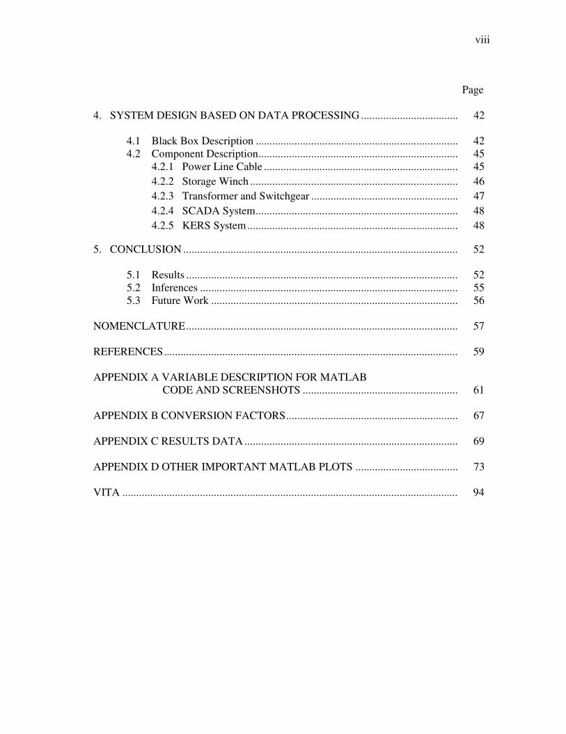
4. SYSTEM DESIGN BASED ON DATA PROCESSING ................................... 42
4.1 Black Box Description ......................................................................... 42 4.2 Component Description ........................................................................ 45
4.2.1 Power Line Cable ...................................................................... 45 4.2.2 Storage Winch ........................................................................... 46 4.2.3 Transformer and Switchgear ..................................................... 47 4.2.4 SCADA System ......................................................................... 48 4.2.5 KERS System ............................................................................ 48
5. CONCLUSION ................................................................................................... 52 5.1 Results .................................................................................................. 52 5.2 Inferences ............................................................................................. 55 5.3 Future Work ......................................................................................... 56 NOMENCLATURE .................................................................................................. 57 REFERENCES .......................................................................................................... 59
APPENDIX A VARIABLE DESCRIPTION FOR MATLAB CODE AND SCREENSHOTS ........................................................ 61
APPENDIX B CONVERSION FACTORS .............................................................. 67
APPENDIX C RESULTS DATA ............................................................................. 69
APPENDIX D OTHER IMPORTANT MATLAB PLOTS ..................................... 73
VITA ......................................................................................................................... 94

ix
LIST OF FIGURES
Page Figure 1 Various sizes of wind turbines with their capital cost ....................... 6 Figure 2 Schematic of fuel cell ........................................................................ 7 Figure 3 Test set up of super capacitor unit ..................................................... 8 Figure 4 Flywheel system coupled with crane’s diesel engine ........................ 10 Figure 5 Cost comparison of various technologies .......................................... 11 Figure 6 LOC 250 rig in actual field ............................................................... 13
Figure 7 Single line diagram of LOC 400 with alternate power system ..................................................................................... 17
Figure 8 Single line diagram of LOC 250 with alternate power system .................................................................................... 19
Figure 9 Flow rate of one of the mud pumps and its variations with time ............................................................................................ 28
Figure 10 Pump pressure vs. time is and its variations ...................................... 30
Figure 11 Instantaneous power of mud pumps vs. time and its variations ...................................................................................... 31
Figure 12 A moving average of window length 2 seconds and actual power curve of the mud pump are plotted vs. time in order to determine transient peaks for this window length ................................................................................... 32 Figure 13 Difference between the actual curve and moving average curve for mud pump vs. time for the window length of 2 seconds ........................................................................................... 33 Figure 14 Difference between the actual power curve and moving average curve combined for mud pumps and top drive vs. time .................... 34 Figure 15 Variation of KERS power requirement with window lengths .......... 35
x
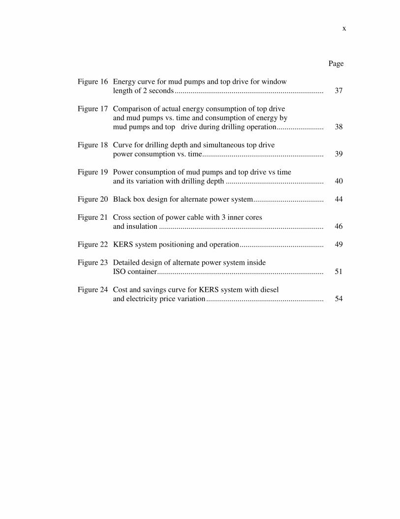
Page Figure 16 Energy curve for mud pumps and top drive for window length of 2 seconds ............................................................................ 37 Figure 17 Comparison of actual energy consumption of top drive and mud pumps vs. time and consumption of energy by mud pumps and top drive during drilling operation ........................ 38
Figure 18 Curve for drilling depth and simultaneous top drive power consumption vs. time .............................................................. 39 Figure 19 Power consumption of mud pumps and top drive vs time and its variation with drilling depth .................................................. 40 Figure 20 Black box design for alternate power system .................................... 44
Figure 21 Cross section of power cable with 3 inner cores and insulation .................................................................................... 46 Figure 22 KERS system positioning and operation ........................................... 49
Figure 23 Detailed design of alternate power system inside ISO container ..................................................................................... 51 Figure 24 Cost and savings curve for KERS system with diesel and electricity price variation ............................................................ 54
xi
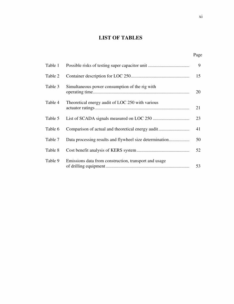
LIST OF TABLES
Page
Table 1 Possible risks of testing super capacitor unit .................................... 9
Table 2 Container description for LOC 250 ................................................... 15 Table 3 Simultaneous power consumption of the rig with operating time .................................................................................... 20
Table 4 Theoretical energy audit of LOC 250 with various actuator ratings .................................................................................. 21 Table 5 List of SCADA signals measured on LOC 250 ................................ 23
Table 6 Comparison of actual and theoretical energy audit ........................... 41
Table 7 Data processing results and flywheel size determination .................. 50
Table 8 Cost benefit analysis of KERS system .............................................. 52
Table 9 Emissions data from construction, transport and usage of drilling equipment ......................................................................... 53
1
1. INTRODUCTION
1.1 Overview
The rig power requirements vary a lot with time and ongoing operation.
Therefore it is in the best interest of operators to research on alternate drilling energy
sources which can make the entire drilling process economic and environmentally
friendly. There are a lot of options available amongst renewable energy resources
namely wind, solar, fuel cells and energy storage devices. Each of these has advantages
and drawbacks in terms of economics or rig footprint. Research into alternate power
systems both economically and practically feasible to modern oil and gas industry can be
very useful. A system of electrical power grid in combination with an energy storage
device such as a flywheel/super capacitor unit is one such source which can provide
substantially cheaper energy as compared to diesel. This energy storage unit can
supply/reuse the power above and below the base load and allow the rigs to draw the
base load either from diesel engines or power grid and hence improve the drilling
efficiency.
1.2 Current Problem
The drilling operation is like driving a car and putting its “pedal to the metal” for
few seconds and releasing it totally again. Drillers seldom pay attention to the power
consumption data making the entire drilling operation fuel inefficient. It is because either
This thesis follows the style of SPE Drilling and Completion.
2
the rigs are not modern enough to capture each and every data point for all the installed
actuators while in operation or the data is tight hole meaning it is kept confidential
during the operation and is destroyed later. There is negligible effort by the industry to
process the rig data in terms of power and energy consumption and improve drilling
efficiency based on that actual data. Same is true for emissions data and rig footprint.
The diesel engines give optimum performance only at a particular value of load.
Intermittent power consumption of the rig poses problems for the diesel engines to reach
that optimum load. The simultaneous power consumption of the rig has to be estimated
and it is certainly not the sum of theoretical power rating of all the installed actuators
(Huisman, 2005). A land rig’s total power consumption is around 2 MW, all of which
comes from diesel engines. These are low on fuel efficiency and produce harmful
emissions because of cycle inefficiency or incomplete combustion (Kumar, Zheng
2008). Hence there is a growing need for developing an environmentally benign
alternate power system which is economic and pragmatic. This study focus into various
alternatives sources of energy storage and come up with a system design based on the
best possible alternative source of energy storage/reuse available.
1.3 Objective
The goal of this project is to determine the feasibility of adopting technology to
reduce the size of the power generating equipment and to provide “peak loading” energy
through the use of new energy generating and energy storage devices.
3
This project is part of a larger Proposed GPRI/Crisman Study to develop
theoretically and empirically an energy inventory of the drilling process from a rig
perspective. There are a number of current technologies that can be used to partially
provide power to a rig and reduce fuel consumption and emissions. These need to be
evaluated technically and economically to determine the feasibility of application to a
drilling rig (e.g., diesel additives, types of fuels (gas, dual fuel system, synthetic fuels
etc, wind energy, solar cells, fuel cells, power management, and gas turbine generators).
Together with these technologies, new energy storage technology (specifically energy
storage compatible with drilling operations) will be required.
Investigation into two peak shaving technologies to be utilized in the drilling rigs
namely flywheels and super capacitors for lightweight rigs. Super capacitors are
potential sources of peak energy which can be instantly discharged to remove transients.
Flywheels offer advantages of reliable operation, instant response, high efficiency, cost
effectiveness and are environmentally friendly with minimal maintenance requirements
(Rojas, 2003). After determination of cost involved for electrically operated rigs, work
will be extended to specification, modeling and layout of electrical systems in the
drilling rigs. This work involves design of a black box which will serve as a link
between power grid and the rig and also incorporate the energy storage/reuse
technology. Attempts will be made to optimize this design in terms of mobility, working
efficiency and cost.

4
2. CHOICE OF ENERGY STORAGE DEVICE
2.1 Available Options
There are quite a number of devices which generate energy. This energy can later
be stored. Solar panels, wind turbines, fuel cells, storage batteries, super capacitors and
flywheels are some of the widely used devices. Apart from these there are also
technologies which are under development phase. The above mentioned devices are
considered viable for this project as they are used worldwide commercially. Energy is
stored differently in all of these devices. In a wind turbine mechanical energy of wind is
converted into electrical energy while in a fuel cell chemical energy is converted into
electrical energy. Each of these energy storage devices is evaluated on the basis of
following factors:
• Size.
• Economics.
• Power generating and storing capability in context of a drilling rig.
• Problems with installation and transport.
• Rig footprint.
2.1.1 Solar PV
A single solar cell unit produce approximately one watt of power.
(www.eere.energy.gov). Solar cells have to be connected in series or parallel connection
to obtain the desired value of power and the discussion of electrical connections of photo
5
voltaic units is beyond the scope of this investigation. By using a solar calculator
application designed by the U.S Department of Energy one can instantly come up with
the cost of entire system in a particular area. The following system was designed which
can provide power to only one of the mud pumps at full load.
Area College Station
Solar Radiance 5.16 kWh/sq m/day
Average Monthly Usage 50,000 kWh
System Size 201.22 kW
Area Required 20122 sq ft.
Estimated Cost $1,609,750 (www.findsolar.com)
Hence, it is economically and practically unrealistic to install such a large unit at
the rig site. It increases rig footprint. Also it is difficult to transport. One other problem
is its dependency on the sun which itself is subjected to intermittent availability. Also
solar cells need a large battery house which again has the constraints of cost and
mobility.
2.1.2 Wind Energy
The wind turbine converts wind energy into rotating motion of the blades. The
turbine is linked with generators through a gear mechanism. The details of the design of
wind turbine are beyond the scope of this investigation. But to have a practical picture
following parameters are obtained from a previous “Environmentally Friendly Drilling”
report.
6
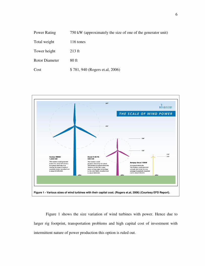
Power Rating 750 kW (approximately the size of one of the generator unit)
Total weight 116 tones
Tower height 213 ft
Rotor Diameter 80 ft
Cost $ 781, 940 (Rogers et.al, 2006)
Figure 1 - Various sizes of wind turbines with their capital cost. (Rogers et.al, 2006) (Courtesy EFD Report).
Figure 1 shows the size variation of wind turbines with power. Hence due to
larger rig footprint, transportation problems and high capital cost of investment with
intermittent nature of power production this option is ruled out.
7
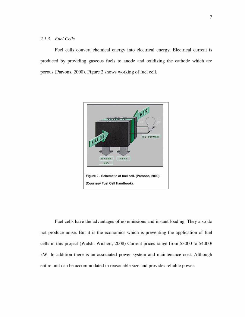
2.1.3 Fuel Cells
Fuel cells convert chemical energy into electrical energy. Electrical current is
produced by providing gaseous fuels to anode and oxidizing the cathode which are
porous (Parsons, 2000). Figure 2 shows working of fuel cell.
Figure 2 - Schematic of fuel cell. (Parsons, 2000)
(Courtesy Fuel Cell Handbook).
Fuel cells have the advantages of no emissions and instant loading. They also do
not produce noise. But it is the economics which is preventing the application of fuel
cells in this project (Walsh, Wichert, 2008) Current prices range from $3000 to $4000/
kW. In addition there is an associated power system and maintenance cost. Although
entire unit can be accommodated in reasonable size and provides reliable power.
8
2.1.4 Storage Battery
Storage battery unit is another viable option in terms of peak shaving. A
stationary sulfur battery at an office park is set up in Ohio which can provide 100 kW of
peak shaving for as much as 30 seconds which is considerably less than the rig
requirements (Tamyurek and Nichols, 2003). Again the economics of the unit and
battery life are restricting factors. In addition batteries fall more into low energy density
systems which is not what is required in this project. This is because of the rig
fluctuations which will cause the battery to partially charge and discharge hundreds of
times in a day. It can adversely affect the battery life which is nearly 15 years or 2500
cycles of full charge and discharge with a cost of $164/ kW (Nichols and Eckroad). Even
after a successful design the battery unit will be a separate entity which will add an extra
container to the rig and hence additional transportation costs.
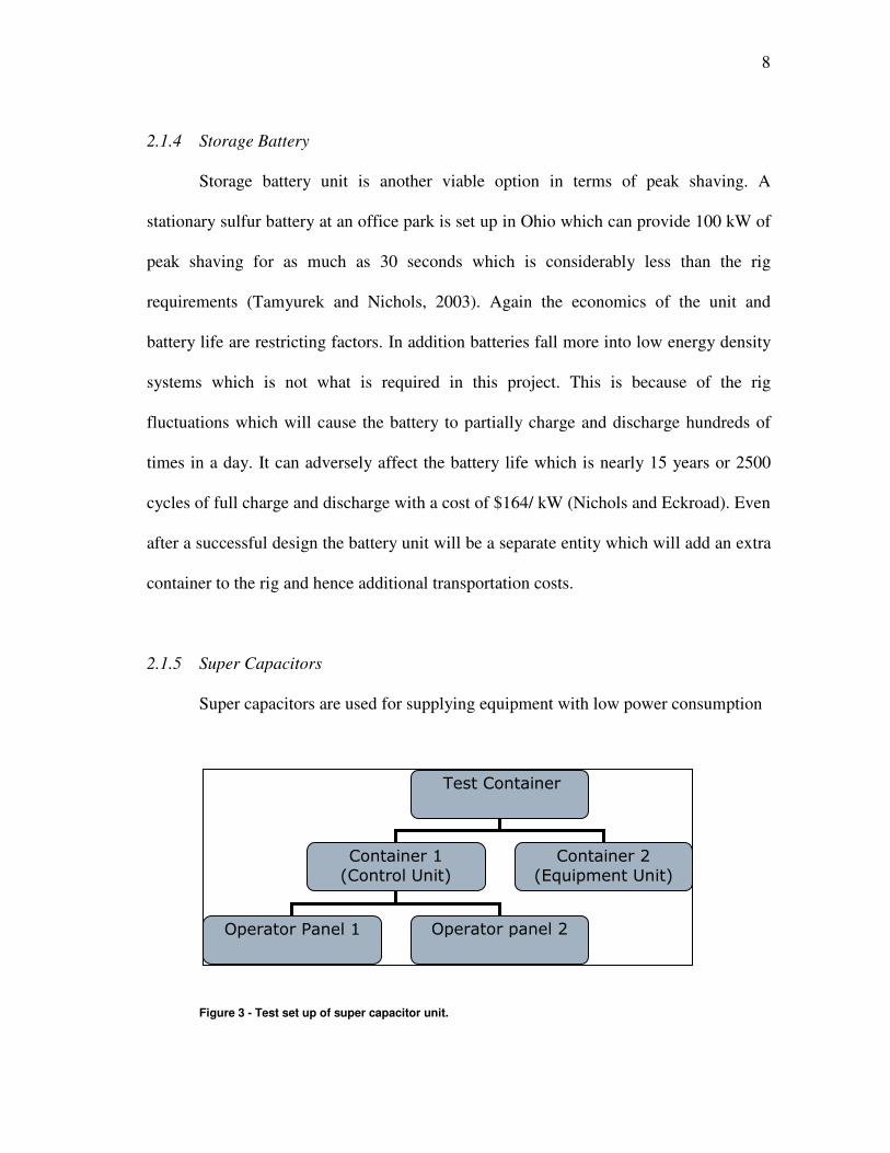
2.1.5 Super Capacitors
Super capacitors are used for supplying equipment with low power consumption
Figure 3 - Test set up of super capacitor unit.
��������������
����������
�������������
����������
��������������
��������������� ���������������
9
and high current requirement with fast charging and discharging time. The test study of
Huisman dealt with 10 modules of 43 capacitors 1500 Farad each (Palthe, 2008).
Figure 3 shows the test set up for super capacitors conducted by Huisman. The test
would be conducted on a 30 kW motor with 5 seconds of hoisting for discharging and
lowering for charging of the ultra capacitor unit. The electrical circuits with converters
and their regulators, communication systems and detailed design of controllers are
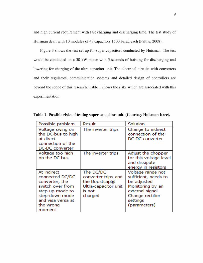
beyond the scope of this research. Table 1 shows the risks which are associated with this
experimentation.
Table 1- Possible risks of testing super capacitor unit. (Courtesy Huisman Itrec).
10
This pilot project is still under testing phase on a small scale of 30 kW and the
results with cost benefit analysis are awaited. This technology has advantages of no
noise, less maintenance and high performance. Therefore efforts are being made to
extend it to drilling rigs.
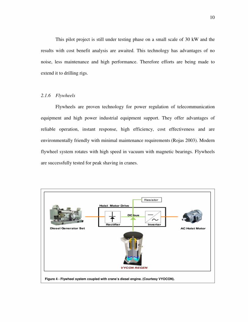
2.1.6 Flywheels
Flywheels are proven technology for power regulation of telecommunication
equipment and high power industrial equipment support. They offer advantages of
reliable operation, instant response, high efficiency, cost effectiveness and are
environmentally friendly with minimal maintenance requirements (Rojas 2003). Modern
flywheel system rotates with high speed in vacuum with magnetic bearings. Flywheels
are successfully tested for peak shaving in cranes.
Figure 4 - Flywheel system coupled with crane’s diesel engine. (Courtesy VYOCON).
11
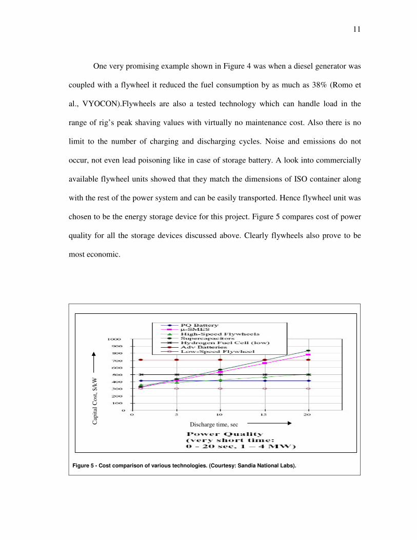
One very promising example shown in Figure 4 was when a diesel generator was
coupled with a flywheel it reduced the fuel consumption by as much as 38% (Romo et
al., VYOCON).Flywheels are also a tested technology which can handle load in the
range of rig’s peak shaving values with virtually no maintenance cost. Also there is no
limit to the number of charging and discharging cycles. Noise and emissions do not
occur, not even lead poisoning like in case of storage battery. A look into commercially
available flywheel units showed that they match the dimensions of ISO container along
with the rest of the power system and can be easily transported. Hence flywheel unit was
chosen to be the energy storage device for this project. Figure 5 compares cost of power
quality for all the storage devices discussed above. Clearly flywheels also prove to be
most economic.
Figure 5 - Cost comparison of various technologies. (Courtesy: Sandia National Labs).
Cap
ital C
ost,
$/kW
Discharge time, sec
12
3. METHODOLOGY
3.1 Stepwise Procedure
1. Read various drilling rig manuals and understood the functioning of rig
components and made a theoretical energy audit by identifying actuators based on
nameplate specifications.
2. Visited a rig site in Texas for interviewing the service engineer and driller to
understand the working and drawbacks of the rig for this new design and gathered
comprehensive time stamped drilling data. Studied emissions produced while
drilling operation.
3. Analyzed and comprehended this data using MATLAB for making an actual
energy audit of the rig. Interview with flywheel expert at Texas A&M University
was done to determine the specifications of flywheel unit.
4. Compared theoretical energy audit with actual audit and designed the optimized
system followed by a cost benefit analysis to determine the return of investment.
5. Designed and encapsulated the power system into the size constraint of ISO
container.
6. Studied diesel engines performance curves to determine exact load which the
energy storage unit has to provide for effective peak shaving.
3.2 Drilling Rig Study
Land Offshore Containerised (LOC) rigs are casing while drilling rigs which
offer a number of advantages like faster drilling time, safe and efficient operation, very
13
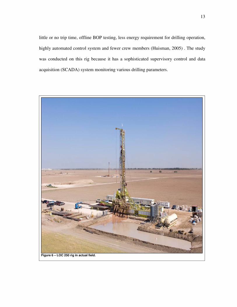
little or no trip time, offline BOP testing, less energy requirement for drilling operation,
highly automated control system and fewer crew members (Huisman, 2005) . The study
was conducted on this rig because it has a sophisticated supervisory control and data
acquisition (SCADA) system monitoring various drilling parameters.
Figure 6 – LOC 250 rig in actual field.
14
A set up of LOC 250 rig in the field is shown in Figure 6. Additionally these are
ISO containerised rigs which means they are easy to relocate and transport. LOC 250
(Land and Offshore Containerized Unit, hook load 250 tonnes) contains 17 containers
while LOC-400 (Land and Offshore Containerized Unit, hook load 400 tonnes) consist
of 16 containers (Huisman, 2005). These are the two Casing While Drilling (CWD) rigs
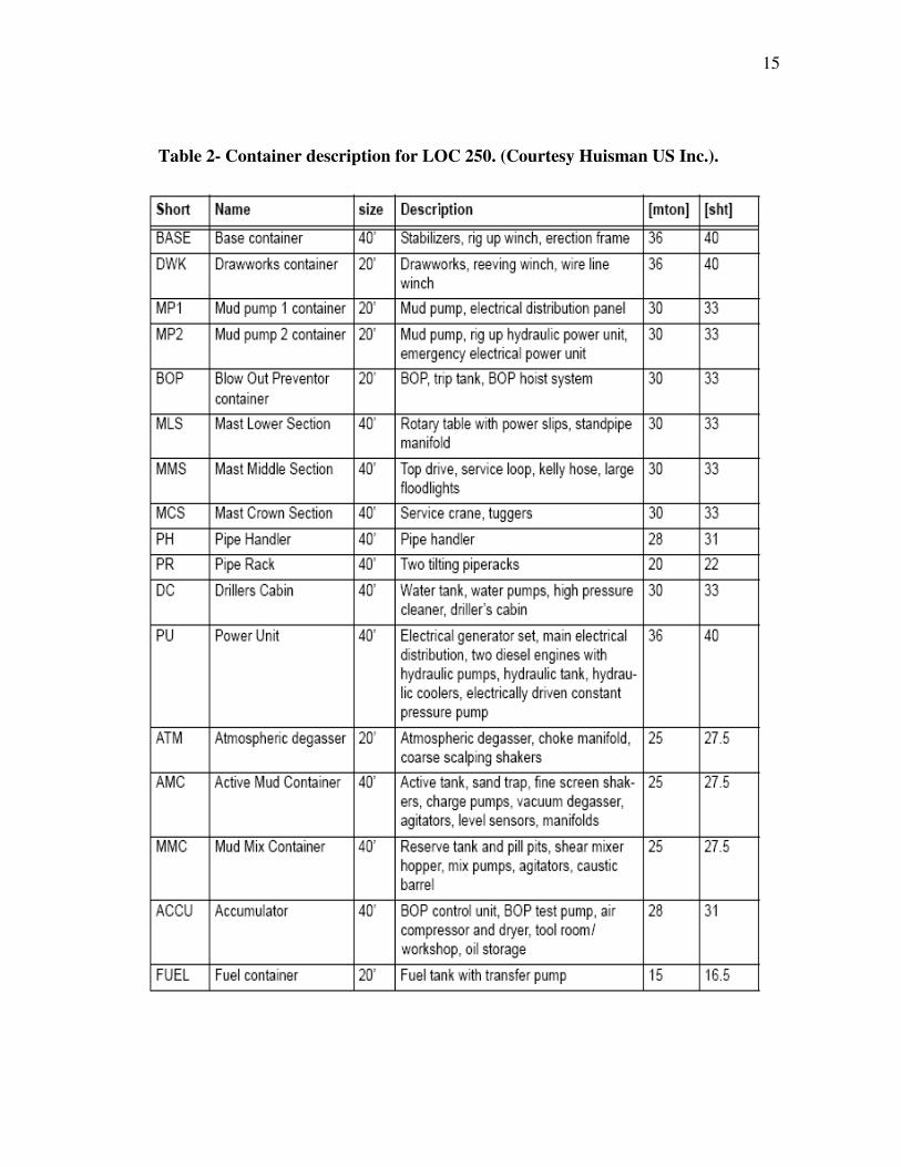
under consideration in this study. Table 2 provides description of various containers of
LOC 250. A comprehensive energy audit of both of these rigs is done in order to
determine the overall power and energy these rigs consume and also the values of
transient power peaks which should be provided by our alternate power system. For this
purpose time stamped data from one of the LOC-250 rig was obtained and processed.
LOC-400 is a successor of LOC-250 and it is assumed that the processed values from
LOC-250 will match closely to that of LOC-400. This is because LOC-400 is an
improved version of LOC-250 and is still under construction. Hence operational data
from LOC-400 is unavailable. Nonetheless theoretical energy audit of LOC-400 is done
in this study.
15
Table 2- Container description for LOC 250. (Courtesy Huisman US Inc.).

16
3.2.1 Electrical System for LOC-400
The main power consumers namely mud pump, drawworks and top drive of
LOC-400 rig are mounted on the main dc bus. There are two or three diesel generators
with total rated power of 2400 KW, 480 V, 60 Hz, 3000 KVA. Two transformers
convert this into 690 V, 60 Hz and feed it to the invertors which then convert it into DC
and supply to the main bus where all major consumers are mounted. Regenerated power
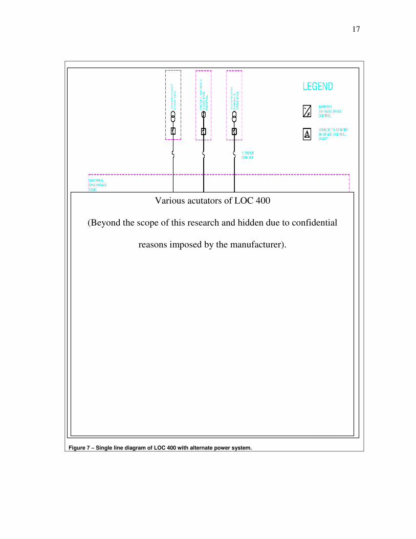
is dissipated in the brake resistors. The single line diagrams for LOC 400 with bus bars
and different actuators and is shown in Figure 7. A close look at the boxes connected to
the main bus shows the two transformer containers which basically forms the alternate
power system. The details of these containers will be described later.
According to Huisman specification manual for LOC-400, it should not be
difficult for the rig to take power from the utility grid. If there are strong reasons in
terms of cost savings and efficiency, such a possibility should be thoroughly explored.
17
Figure 7 – Single line diagram of LOC 400 with alternate power system.
Various acutators of LOC 400
(Beyond the scope of this research and hidden due to confidential
reasons imposed by the manufacturer).
18
3.2.2 Electrical System for LOC-250
There are two generators feeding the 480 V main bus which itself feeds the
hydraulic power unit (HPU) and one generator feeding electrical power unit (EPU).
Variable frequency drives are mounted in order to attain different speeds. There are no
invertors feeding the main power consumers rather they are AC motors as opposed to
LOC-400. The hydraulic power system in LOC-250 is replaced by electrical system in
LOC-400 which is the reason why it is considered to be a better version of LOC-250.
Also this is one of the reasons why there is no efficiency loss in LOC-400 when
converting the regenerative power from hydraulic to mechanical and then electrical
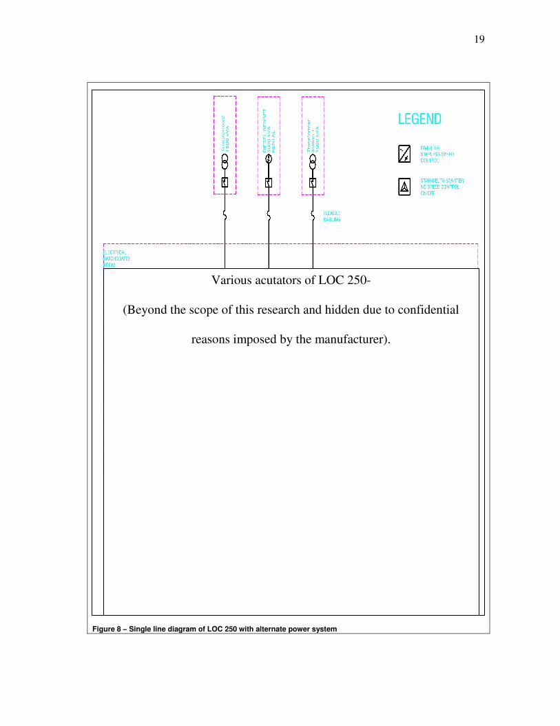
which is the case with LOC-250. The single line diagram for LOC 250 with bus bars and
different actuators in place is shown in Figure 8. Some of the actuators installed are not
shown in the single line diagram because of confidential reasons. However they do not
pertain to the scope of this project and hence not required by the reader to know.
19
Figure 8 – Single line diagram of LOC 250 with alternate power system
Various acutators of LOC 250-
(Beyond the scope of this research and hidden due to confidential
reasons imposed by the manufacturer).
20
3.3 Energy Audit
3.3.1 Theoretical Energy Audit
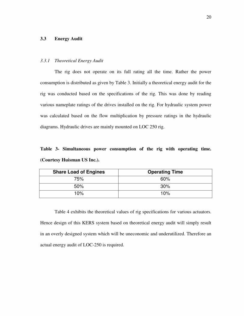
The rig does not operate on its full rating all the time. Rather the power
consumption is distributed as given by Table 3. Initially a theoretical energy audit for the
rig was conducted based on the specifications of the rig. This was done by reading
various nameplate ratings of the drives installed on the rig. For hydraulic system power
was calculated based on the flow multiplication by pressure ratings in the hydraulic
diagrams. Hydraulic drives are mainly mounted on LOC 250 rig.
Table 3- Simultaneous power consumption of the rig with operating time.
(Courtesy Huisman US Inc.).
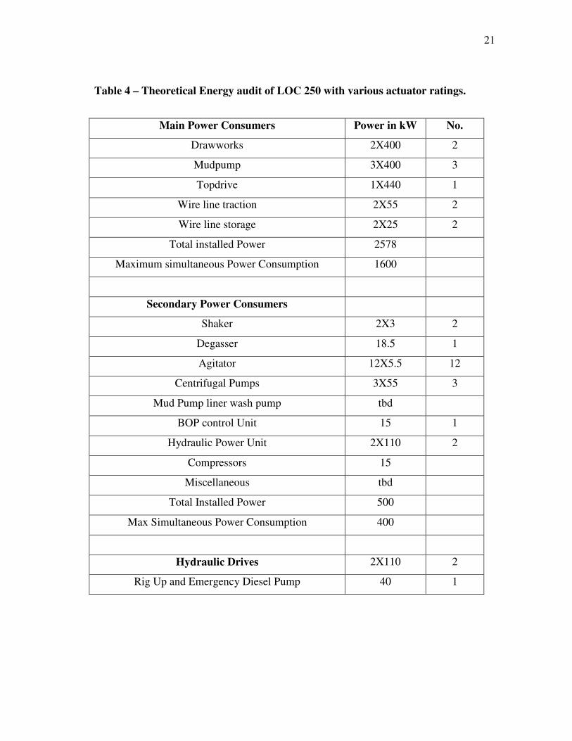
Table 4 exhibits the theoretical values of rig specifications for various actuators.
Hence design of this KERS system based on theoretical energy audit will simply result
in an overly designed system which will be uneconomic and underutilized. Therefore an
actual energy audit of LOC-250 is required.
Share Load of Engines Operating Time 75% 60% 50% 30% 10% 10%
21
Table 4 – Theoretical Energy audit of LOC 250 with various actuator ratings.
Main Power Consumers Power in kW No.
Drawworks 2X400 2
Mudpump 3X400 3
Topdrive 1X440 1
Wire line traction 2X55 2
Wire line storage 2X25 2
Total installed Power 2578
Maximum simultaneous Power Consumption 1600
Secondary Power Consumers
Shaker 2X3 2
Degasser 18.5 1
Agitator 12X5.5 12
Centrifugal Pumps 3X55 3
Mud Pump liner wash pump tbd
BOP control Unit 15 1
Hydraulic Power Unit 2X110 2
Compressors 15
Miscellaneous tbd
Total Installed Power 500
Max Simultaneous Power Consumption 400
Hydraulic Drives 2X110 2
Rig Up and Emergency Diesel Pump 40 1
22
3.3.2 Actual Energy Audit
To obtain a realistic measure of power consumption an actual audit of the rig is
required. This can be done by processing real time operational rig data. The process
starts with gathering the rig data from its SCADA system. This data can be converted to
comma separated format by the use of Trend Reader software. These comma separated
files after a little conditioning can be imported to MATLAB. There were as much as 23
rig parameters obtained from SCADA system. Each of these parameters was as much as
1.3 million lines long. Excel can process data only a little more than 65000 lines. Hence
a comprehensive tool with multiple functionalities was required. This is the reason why
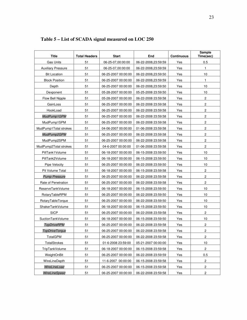
MATLAB was chosen for this research. Table 5 shows various rig parameters. The
highlighted parameters were those signals which were later combined in MATLAB for
obtaining relevant results.
23
Table 5 – List of SCADA signal measured on LOC 250
Title Total Headers Start End Continuous Sample
Time(sec)
Gas Units 51 06-25-07,00:00:00 06-22-2008,23:59:59 Yes 0.5
Auxiliary Pressure 51 06-25-07,00:00:00 06-22-2008,23:59:59 Yes 1
Bit Location 51 06-25-2007 00:00:00 06-22-2008,23:59:50 Yes 10
Block Position 51 06-25-2007 00:00:00 06-22-2008,23:59:59 Yes 1
Depth 51 06-25-2007 00:00:00 06-22-2008,23:59:50 Yes 10
Dexponent 51 05-28-2007 00:00:00 05-25-2008 23:59:50 Yes 10
Flow Bell Nipple 51 05-28-2007 00:00:00 06-22-2008 23:59:58 Yes 2
GainLoss 51 06-25-2007 00:00:00 06-22-2008 23:59:58 Yes 2
HookLoad 51 06-25-2007 00:00:00 06-22-2008 23:59:58 Yes 2
MudPump1GPM 51 06-25-2007 00:00:00 06-22-2008 23:59:58 Yes 2
MudPump1SPM 51 06-25-2007 00:00:00 06-22-2008 23:59:58 Yes 2
MudPump1Total strokes 51 04-06-2007 00:00:00 01-06-2008 23:59:58 Yes 2
MudPump2GPM 51 06-25-2007 00:00:00 06-22-2008 23:59:58 Yes 2
MudPump2SPM 51 06-25-2007 00:00:00 06-22-2008 23:59:58 Yes 2
MudPump2Total strokes 51 04-6-2007 00:00:00 01-06-2008 23:59:58 Yes 2
PillTank1Volume 51 06-18-2007 00:00:00 06-15-2008 23:59:50 Yes 10
PillTank2Volume 51 06-18-2007 00:00:00 06-15-2008 23:59:50 Yes 10
Pipe Velocity 51 06-25-2007 00:00:00 06-22-2008 23:59:50 Yes 10
Pit Volume Total 51 06-18-2007 00:00:00 06-15-2008 23:59:58 Yes 2
Pump Pressure 51 06-25-2007 00:00:00 06-22-2008 23:59:58 Yes 2
Rate of Penetration 51 06-25-2007 00:00:00 06-22-2008 23:59:58 Yes 2
ReserveTankVolume 51 06-18-2007 00:00:00 06-15-2008 23:59:50 Yes 10
RotaryTableRPM 51 06-25-2007 00:00:00 06-22-2008 23:59:50 Yes 10
RotaryTableTorque 51 06-25-2007 00:00:00 06-22-2008 23:59:50 Yes 10
ShakerTankVolume 51 06-18-2007 00:00:00 06-15-2008 23:59:50 Yes 10
SICP 51 06-25-2007 00:00:00 06-22-2008 23:59:58 Yes 2
SuctionTankVolume 51 06-18-2007 00:00:00 06-15-2008 23:59:50 Yes 10
TopDriveRPM 51 06-25-2007 00:00:00 06-22-2008 23:59:58 Yes 2
TopDriveTorque 51 06-25-2007 00:00:00 06-22-2008 23:59:58 Yes 2
TotalGPM 51 06-25-2007 00:00:00 06-22-2008 23:59:58 Yes 2
TotalStrokes 51 01-6-2008 23:59:00 05-21-2007 00:00:00 Yes 10
TripTankVolume 51 06-18-2007 00:00:00 06-15-2008 23:59:58 Yes 2
WeightOnBit 51 06-25-2007 00:00:00 06-22-2008 23:59:59 Yes 0.5
WireLineDepth 51 11-6-2007 00:00:00 06-15-2008 23:59:58 Yes 2
WireLineLoad 51 06-25-2007 00:00:00 06-15-2008 23:59:58 Yes 2
WireLineSpeed 51 06-25-2007 00:00:00 06-22-2008 23:59:58 Yes 2

24
3.3.3 MATLAB Code
The following procedure was followed in MATLAB:
• [date,time,mp1gpmdatadata]=textread['C:\Users\ankit\Desktop\Signal
combination\MudPump1GPM.txt','%s%s%n'];
• [date,time,ppdata]=textread['C:\Users\ankit\Desktop\Signal
combination\PumpPressure.txt','%s%s%n'];
• %Delete date and time for both of the above
• plot(mp1gpmdata);
• plot(ppdata);
• mppower=mp1gpmdata.*ppdata;%point wise vector multiplication
• plot(mppower);
• mpmv=filter(ones(1,2)/2,1,mppower);%Moving Average for 2 seconds
• plot(mpmv);%Plotting moving average curve
• z=[1:1330000]%defining a column vector z
• z=z';
• plot(z,mppower,z,mpmv);%plotting original curve VS moving average curve
• mpdifference=mppower(2:1330000,1)-mpmv(1:1329999,1);%Calculating the
difference between the two curves with 2 seconds lag
• plot(mpdifference*.0063);%plotting difference between original signal and
moving average on KW scale
• mpdifference1=mpdifference(4e5:6e5)%segmenting a part of 'difference'
• mpdifference1=mpdifference1*.0063%converting into KW scale

25
• mpenergy1=filter(ones(1,200001)/1,1,mpdifference1);%adding Nth value to all
(N-1) values for obtaining energy curve
• %Entire procedure is repeated for top drive with a conversion factor of
.00010046
• plot(mpdifference(1:1309725)+mp2difference(1:1309725)+tddifference);%plotti
ng total difference of power for mud pump1,mud pump2 and top drive which the
flywheel has to supply(2 sec)
• plot(z(200001:400001),mpenergy1,z(400001:600001),mpenergy2,z(600001:800
001),mpenergy3);%Plotting overall energy for mud pump1
• %Remove the offset from above curve
• plot(z(200001:400001),mp2energy1,z(400001:600001),mp2energy2,z(600001:8
00001),mp2energy3);%Plotting energy for mud pump2
• %Remove the offset from above curve
• plot(z(200001:400001),tdenergy1,z(400001:600001),tdenergy2,z(600001:80000
1),tdenergy3);%Plotting cumulative energy for top drive
• % Remove the offset from above curve
• plot(mpdifference(1:1309733)+mp2difference(1:1309733)+tddifference);%Plotti
ng total difference of power for mud pump1,mud pump2,top drive for 2 sec
• plot(z(200001:400001),mpenergy1,'b',z(400001:600001),mpenergy2,'b',z(600001
:800001),mpenergy3,'b',z(200001:400001),mp2energy1,'g',z(400001:600001),mp
2energy2,'g',z(600001:800001),mp2energy3,'g',z(200001:400001),tdenergy1,'y',z
26
(400001:600001),tdenergy2,'y',z(600001:800001),tdenergy3,'y');%Comparing
energy curves for mud pump1,2 and top drive
• plot(z(4e5:6e5),mp2energy1+mpenergy1+tdenergy1,z(6e5:8e5),mp2energy2+mp
energy2+tdenergy2,z(8e5:10e5),mp2energy3+mpenergy3+tdenergy3);
• grid %Adding energy curves for mud pump1,2 and top drive
• %maximum value of cumulative energy curve for 2 sec=550KJ; Including an
efficiency factor of 0.7 for the entire system E max(flywheel)=785 KJ
• %maximum value of difference of power curve for 2 sec =100 KW; Including an
efficiency factor of 0.7 for the entire system P max (flywheel)=143 KW
• %entire procedure is repeated for window period of 10 seconds
• %maximum value of cumulative energy curve for 10 sec=20000KJ;Including an
efficiency factor of 0.7 for the entire system E max (flywheel)=28570 KJ
• %maximum value of difference of power curve for 10 sec =140 KW; Including
an efficiency factor of 0.7 for the entire system P max (flywheel)=200 KW
• %entire procedure is repeated for window period of 20 seconds
• %maximum value of cumulative energy curve for 20 sec,=86000KJ;Including an
efficiency factor of 0.7 for the entire system E max (flywheel)=122857 KJ
• %maximum value of difference of power curve for 20 sec=152 KW; Including
an efficiency factor of 0.7 for the entire system P max (flywheel)= 217 KW
• plot(z(200001:400001),mpenergy1,z(400001:600001),mpenergy2,z(600001:800
001),mpenergy3,z(200001:400001),tdenergy1,z(400001:600001),tdenergy2,z(60

27
0001:800001),tdenergy3)%Comparing Cumulative Energy Curves for Mud
Pump and Top Drive for all window lengths
3.3.4 Simplified Description of MATLAB Code
An easier description for MATLAB code follows. For various variable names
refer to Appendix A:
• Import the text file data in MATLAB by using either import wizard or textread
command. Say data for Mud Pump is imported.
• Three vectors namely date, time and data are formed. As MATLAB plots the
data VS index by default and index can be scaled to sample time we can delete
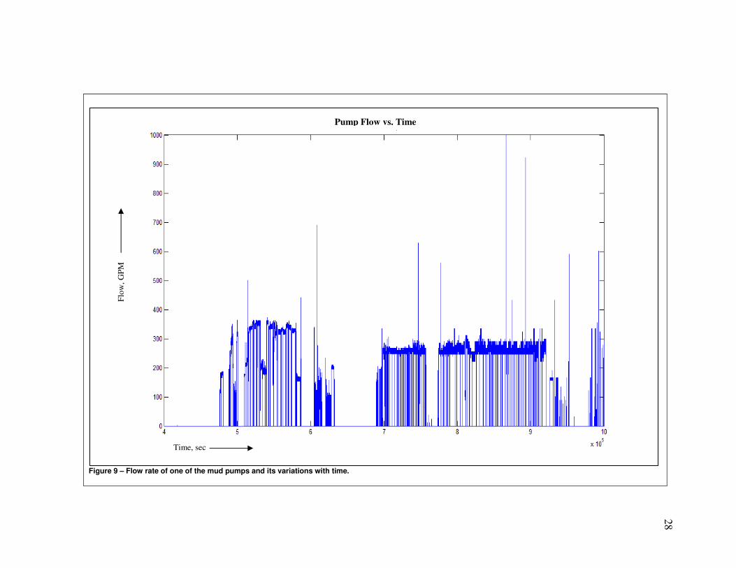
the date and time vectors for simplicity. Plot the Mud Pump Flow VS Time�
(Figure 9).
• Vector mpdata is ready to use. A similar procedure is followed for pump pressure
data to obtain and plot ppdata vector (Figure 10).
28
Figure 9 – Flow rate of one of the mud pumps and its variations with time.
Flow
, GPM
Time, sec
Pump Flow vs. Time
29
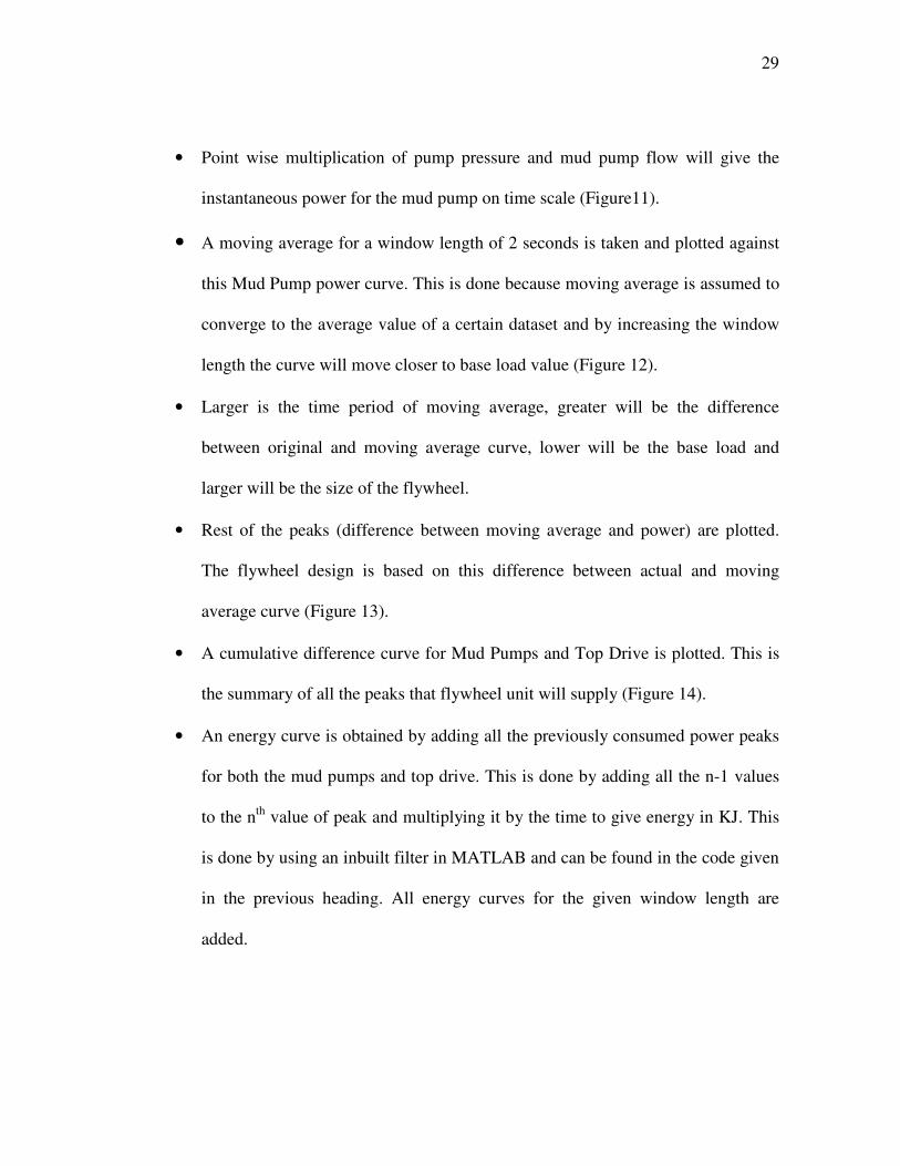
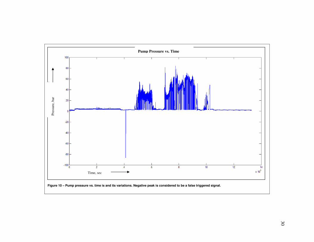
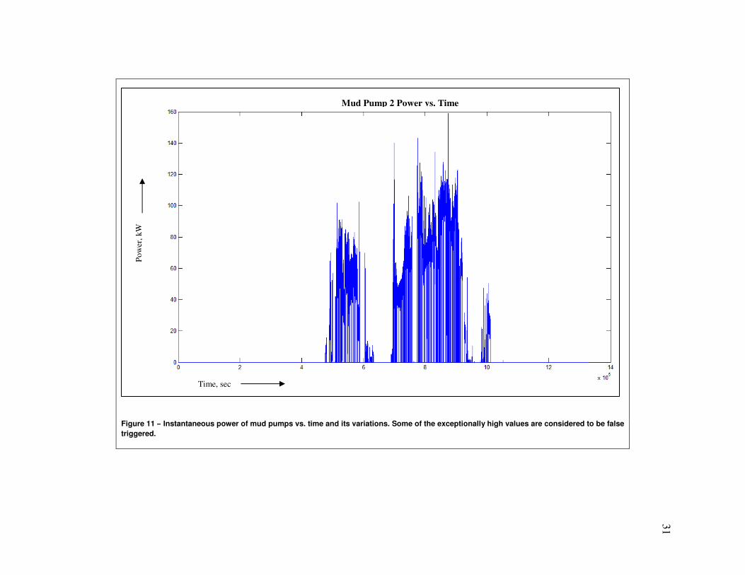
• Point wise multiplication of pump pressure and mud pump flow will give the
instantaneous power for the mud pump on time scale (Figure11).
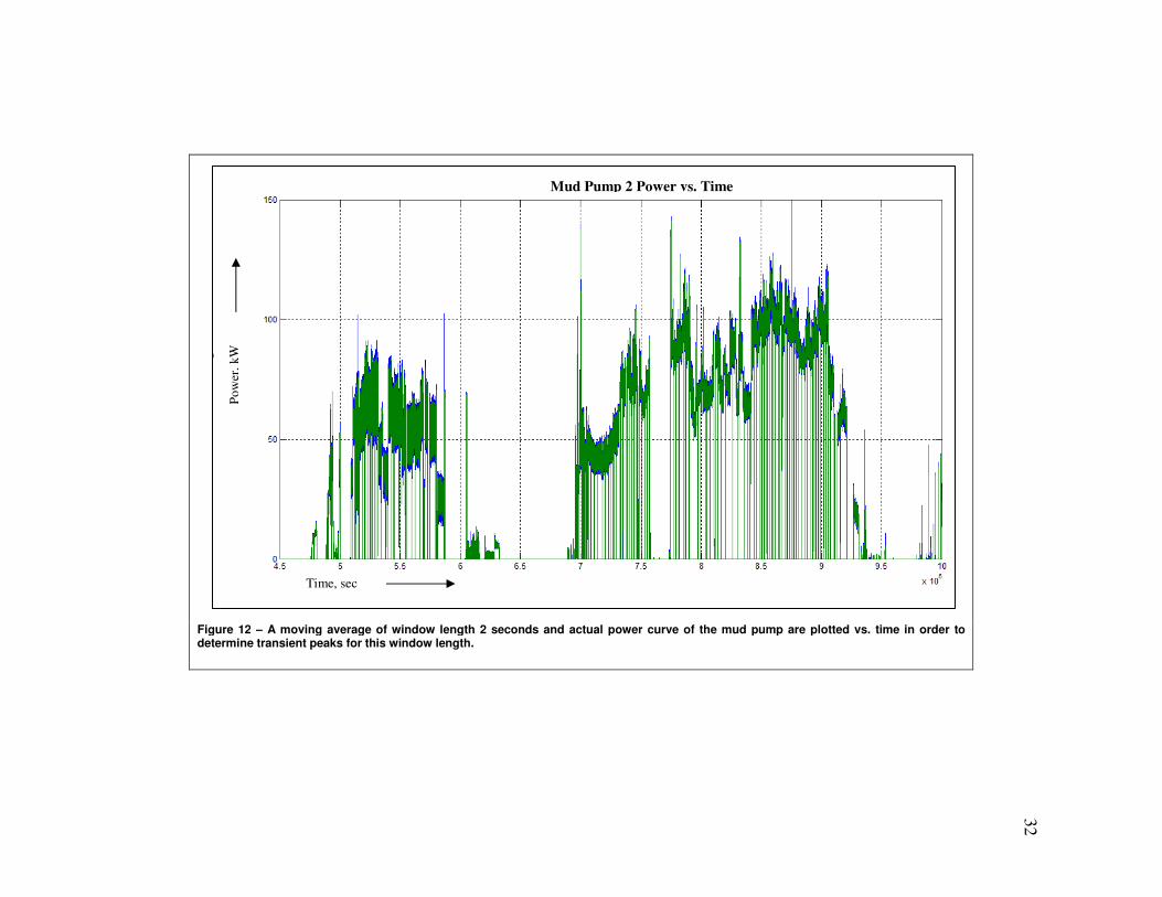
• A moving average for a window length of 2 seconds is taken and plotted against
this Mud Pump power curve. This is done because moving average is assumed to
converge to the average value of a certain dataset and by increasing the window
length the curve will move closer to base load value (Figure 12).
• Larger is the time period of moving average, greater will be the difference
between original and moving average curve, lower will be the base load and
larger will be the size of the flywheel.
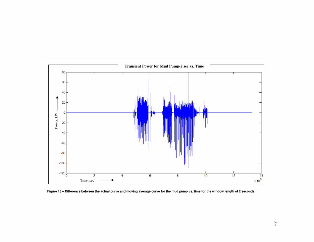
• Rest of the peaks (difference between moving average and power) are plotted.
The flywheel design is based on this difference between actual and moving
average curve (Figure 13).
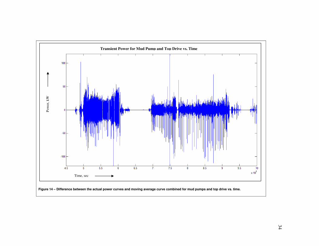
• A cumulative difference curve for Mud Pumps and Top Drive is plotted. This is
the summary of all the peaks that flywheel unit will supply (Figure 14).
• An energy curve is obtained by adding all the previously consumed power peaks
for both the mud pumps and top drive. This is done by adding all the n-1 values
to the nth value of peak and multiplying it by the time to give energy in KJ. This
is done by using an inbuilt filter in MATLAB and can be found in the code given
in the previous heading. All energy curves for the given window length are
added.
30
Figure 10 – Pump pressure vs. time is and its variations. Negative peak is considered to be a false triggered signal.
Time, sec
Pres
sure
, bar
Pump Pressure vs. Time
31
Figure 11 – Instantaneous power of mud pumps vs. time and its variations. Some of the exceptionally high values are considered to be false triggered.
Pow
er, k
W
Time, sec
Mud Pump 2 Power vs. Time
32
Figure 12 – A moving average of window length 2 seconds and actual power curve of the mud pump are plotted vs. time in order to determine transient peaks for this window length.
Time, sec
Pow
er, k
W
Mud Pump 2 Power vs. Time
33
Figure 13 – Difference between the actual curve and moving average curve for the mud pump vs. time for the window length of 2 seconds.
Pow
er, k
W
Time, sec
Transient Power for Mud Pump-2 sec vs. Time
34
Figure 14 – Difference between the actual power curves and moving average curve combined for mud pumps and top drive vs. time.
Pow
er, k
W
Time, sec
Transient Power for Mud Pump and Top Drive vs. Time
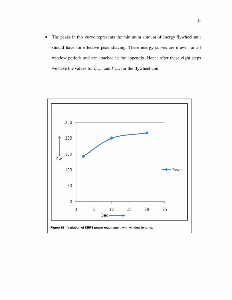
• The peaks in this curve represents the minimum amount of energy flywheel unit
should have for effective peak shaving. These energy curves are drawn for all
window periods and are attached in the appendix. Hence after these eight steps
we have the values for E max and P max for the flywheel unit.
Figure 15 – Variation of KERS power requirement with window lengths.
35
Hence after a rigorous data processing we come up with the moving maximum power
and maximum energy values which the flywheel unit has to provide in order to be
effective for peak shaving. Figure 15 show variations of the value of power which
increases with the increasing window length.
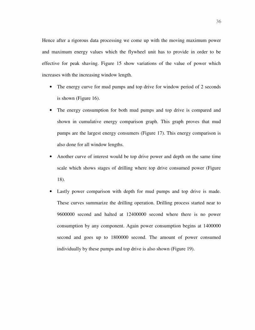
• The energy curve for mud pumps and top drive for window period of 2 seconds
is shown (Figure 16).
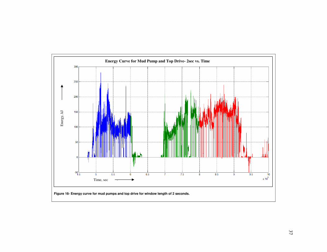
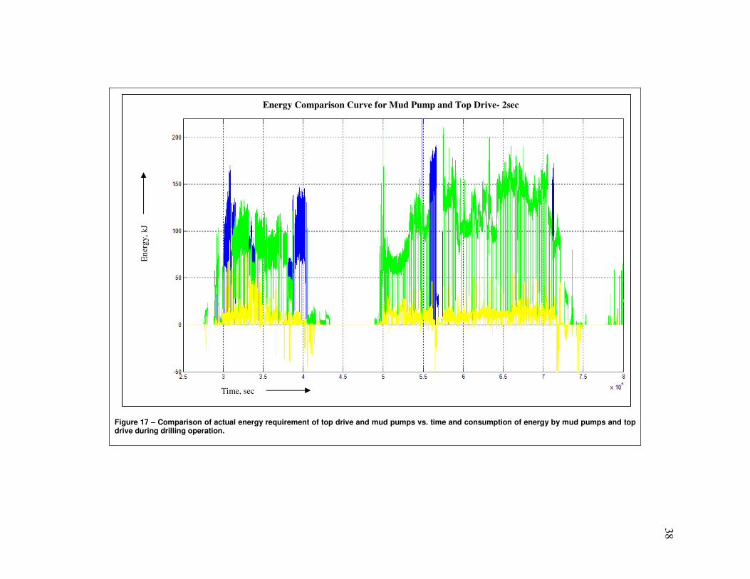
• The energy consumption for both mud pumps and top drive is compared and
shown in cumulative energy comparison graph. This graph proves that mud
pumps are the largest energy consumers (Figure 17). This energy comparison is
also done for all window lengths.
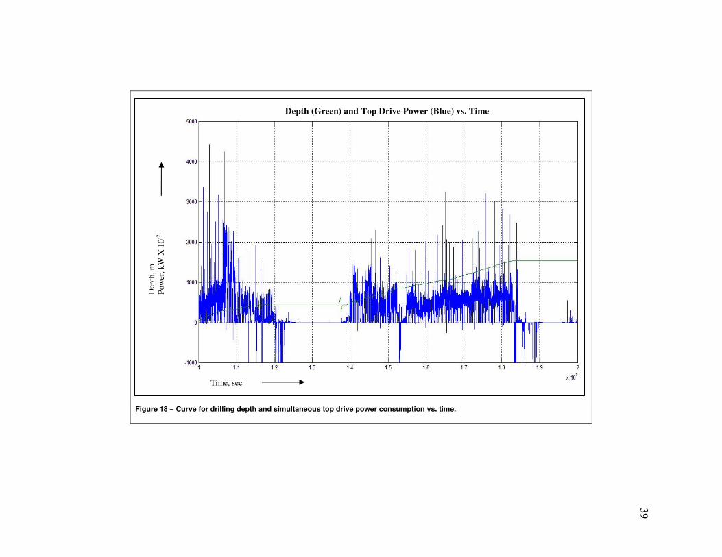
• Another curve of interest would be top drive power and depth on the same time
scale which shows stages of drilling where top drive consumed power (Figure
18).
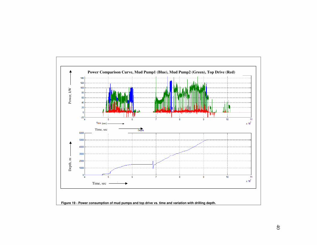
• Lastly power comparison with depth for mud pumps and top drive is made.
These curves summarize the drilling operation. Drilling process started near to
9600000 second and halted at 12400000 second where there is no power
consumption by any component. Again power consumption begins at 1400000
second and goes up to 1800000 second. The amount of power consumed
individually by these pumps and top drive is also shown (Figure 19).
36
37
Figure 16- Energy curve for mud pumps and top drive for window length of 2 seconds.
Ene
rgy,
kJ
Time, sec
Energy Curve for Mud Pump and Top Drive- 2sec vs. Time
38
Figure 17 – Comparison of actual energy requirement of top drive and mud pumps vs. time and consumption of energy by mud pumps and top drive during drilling operation.
Ene
rgy,
kJ
Time, sec
Energy Comparison Curve for Mud Pump and Top Drive- 2sec
39
Figure 18 – Curve for drilling depth and simultaneous top drive power consumption vs. time.
Dep
th, m
Po
wer
, kW
X 1
0-2
Time, sec
Depth (Green) and Top Drive Power (Blue) vs. Time
40
Figure 19 - Power consumption of mud pumps and top drive vs. time and variation with drilling depth.
Pow
er, k
W
Dep
th, m
Time, sec
Time, sec
Power Comparison Curve, Mud Pump1 (Blue), Mud Pump2 (Green), Top Drive (Red)
41�
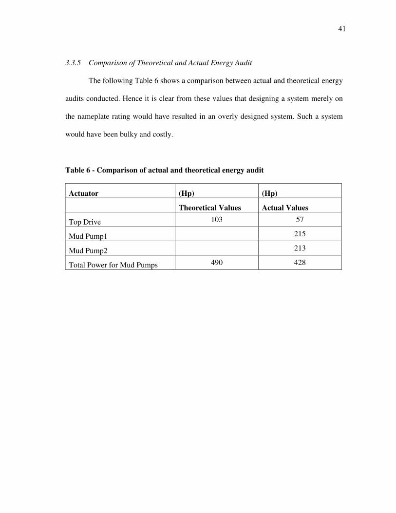
3.3.5 Comparison of Theoretical and Actual Energy Audit
The following Table 6 shows a comparison between actual and theoretical energy
audits conducted. Hence it is clear from these values that designing a system merely on
the nameplate rating would have resulted in an overly designed system. Such a system
would have been bulky and costly.
Table 6 - Comparison of actual and theoretical energy audit
Actuator (Hp) (Hp)
Theoretical Values Actual Values
Top Drive 103 57
Mud Pump1 215
Mud Pump2 213
Total Power for Mud Pumps 490 428

42�
4. SYSTEM DESIGN BASED ON DATA PROCESSING
This section will illustrate the important components of alternate power system
and their corresponding description. All of design mentioned here is based on the rig
specification and data processing results.
4.1 Black Box Description
Initially the power system under design is assumed to be a black box. Following
important points are considered before designing any component:
• Efficient Operation
Design should be such that all kind of losses should be minimized. This includes
T&D losses and all transformer losses.
• Reliable
The possibility of total equipment breakdown should be negligible. Two
transformers with a back up diesel generator add to the redundancy. Even if all
the three fails the emergency rig up power can be used which itself can be
operated from an energy storage device like flywheel or a super capacitor unit.
• Cost Effective
In order for the system to be lucrative to operators, initial cost incurred should be
minimal. With fluctuating gas prices, drilling with electricity can be economical.
The goal will be to make this design much cheaper as compared to diesel fed rig.
• Safe Operation

43�
Risk of shocks or accidents should be minimized. Huisman standards will be
incorporated. Some of these measures include:
1. Equipment provided for protection of persons at work near electrical
installations.
2. Equipment ability to bear electrical stresses and shocks.
3. Bus bar protection.
4. Protection from excess/short circuit current.
5. Cut off and isolation.
6. Working conditions, lighting, competent personal.
7. Protection against indirect contact.
8. Adequate earthing requirements.
• Mobile
A mobile unit can reduce great deal of operator reluctance for transportation and
set up. The switchbox dimensions will be decided so as to fit it in a 20 ft or 40 ft
ISO standard container.
• Remote Operation
The existing SCADA system on LOC 400 will be used to operate the transformer
unit remotely and to monitor various predefined parameters.
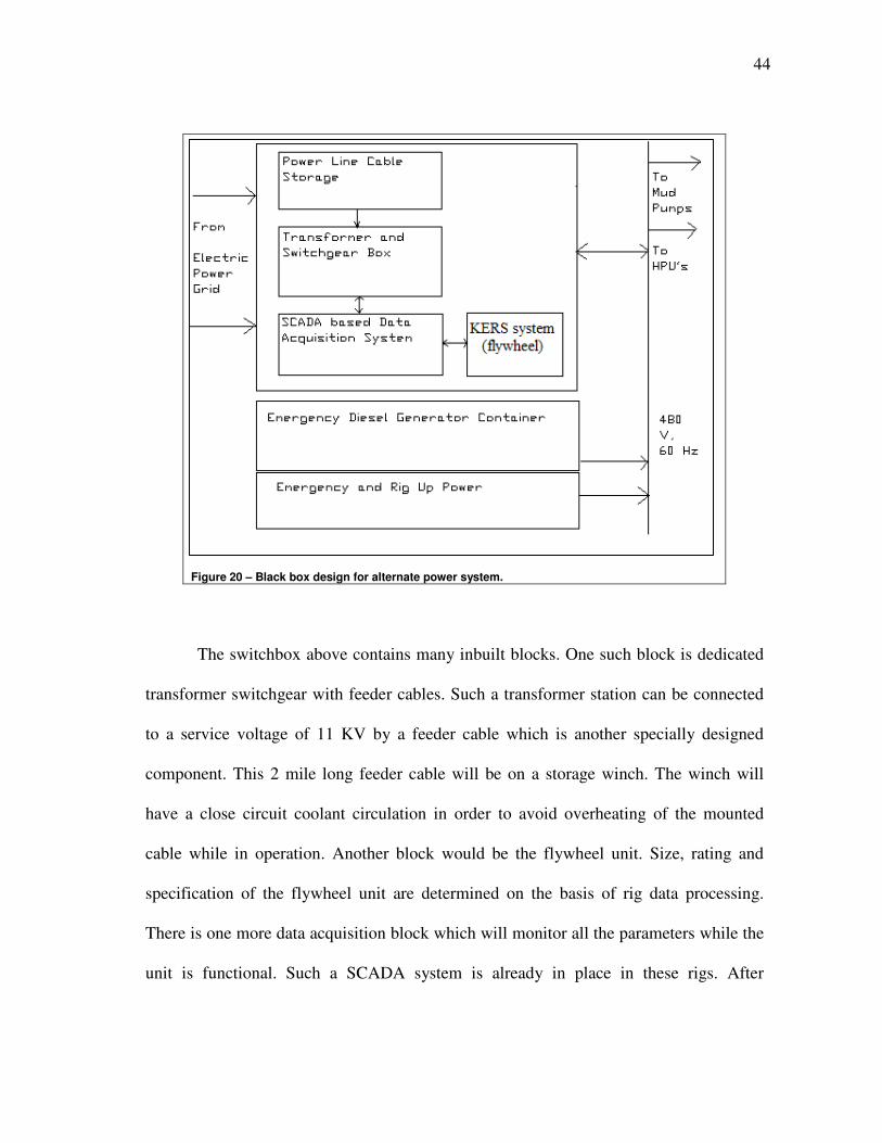
A black box design is illustrated in Figure 19 considering all of the above factors.
This diagram shows constituent components of the black box. A brief description of the
black box design is also given following the diagram.
44�
The switchbox above contains many inbuilt blocks. One such block is dedicated
transformer switchgear with feeder cables. Such a transformer station can be connected
to a service voltage of 11 KV by a feeder cable which is another specially designed
component. This 2 mile long feeder cable will be on a storage winch. The winch will
have a close circuit coolant circulation in order to avoid overheating of the mounted
cable while in operation. Another block would be the flywheel unit. Size, rating and
specification of the flywheel unit are determined on the basis of rig data processing.
There is one more data acquisition block which will monitor all the parameters while the
unit is functional. Such a SCADA system is already in place in these rigs. After
Figure 20 – Black box design for alternate power system.

45�
appropriate size determination all of these blocks will be placed in a 20 ft or 40 ft closed
ISO container which has the inherent advantage of easy transportation with no special
freight regulations. The overall system also contains emergency back up diesel generator
unit in case the electrical design fails or power trips. A detailed design with dimensions
will be shown later.
4.2 Component Description
4.2.1 Power Line Cable
Assuming an overall derating factor of 0.6 for ground (including air and ground
temperatures, grouping of cables, depth of burial, overall derating factors for ground and
air) ( McAllister 1987) and calculating the transformer primary winding current for 3.3
MVA loading. The equation governing the primary current is given by:
I p = 3300000/ (�3 X 11000) = 173.4 Amps…………………………..Equation 1
where I p is the primary winding current.
Cable equivalent current for 25 ‘C = 173.4/0.6= 289.01 Amps………Equation 2
This value corresponds to a 3 core cable with cross sectional area of 95 mm2 and
outer core diameter of 12 mm in standard tables in the cable handbook (Fink and Beaty
1987).Thus the overall diameter of the cable would be 36 mm (Figure 13). This cable
might be oil cooled from within. Environmental regulations governing laying this high
46�
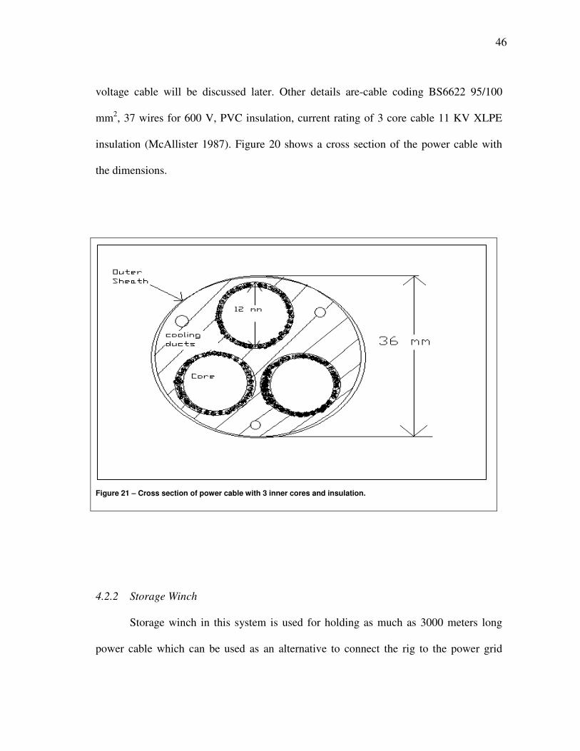
voltage cable will be discussed later. Other details are-cable coding BS6622 95/100
mm2, 37 wires for 600 V, PVC insulation, current rating of 3 core cable 11 KV XLPE
insulation (McAllister 1987). Figure 20 shows a cross section of the power cable with
the dimensions.
4.2.2 Storage Winch
Storage winch in this system is used for holding as much as 3000 meters long
power cable which can be used as an alternative to connect the rig to the power grid
Figure 21 – Cross section of power cable with 3 inner cores and insulation.
47�
instead of constructing power lines to drill site. This winch has to be accommodated into
2.2 meter height and width dimension of ISO container. The winch’s main design
parameters are wire diameter 36 mm, drum wire storage 3042 m, number of safety
windings 3, number of layers 16, drum diameter in groove 640 mm, length of the drum
2200 mm, ratio of wire/ drum diameter 17.78, pitch of the drum 37.44 mm.
4.2.3 Transformer and Switchgear
3 Phase, distribution type,11 KV/480 V,60 Hz, Class F,DZ. 2 transformers will
be needed to replace either of the diesel engines. Incoming and bus bar section circuit
breakers should be 3/4 pole for low voltage based on air break. For high voltage they
should be either SF6 or vacuum based. Earthing bars should be high grade copper located
at front or rear enclosure, screen clamping type. Standard lightning arrestor and cabinet
cooling system is also recommended (Alstom T&D Protection and Control 1995). Main
bus bar is 400 amps, high grade copper (Westinghouse Electric Cooperation 1964).
Control and indicators include power factor meter, voltmeter, ammeter, frequency meter,
synchronising devices and varmeter. Fuses are in series with contactor with rating of
1.5~2 times normal load current. Standards for safety vary from designer to designer and
the manufacturer. Detailed design is left up to the electrical design and installation
company and superior quality equipment or equipment with industry wide standard
usage is recommended.
48�
4.2.4 SCADA System
Same as currently installed to measure all the drilling parameters. In addition a
feature of measuring power and current usage and transient could be included for
obtaining additional data sets.
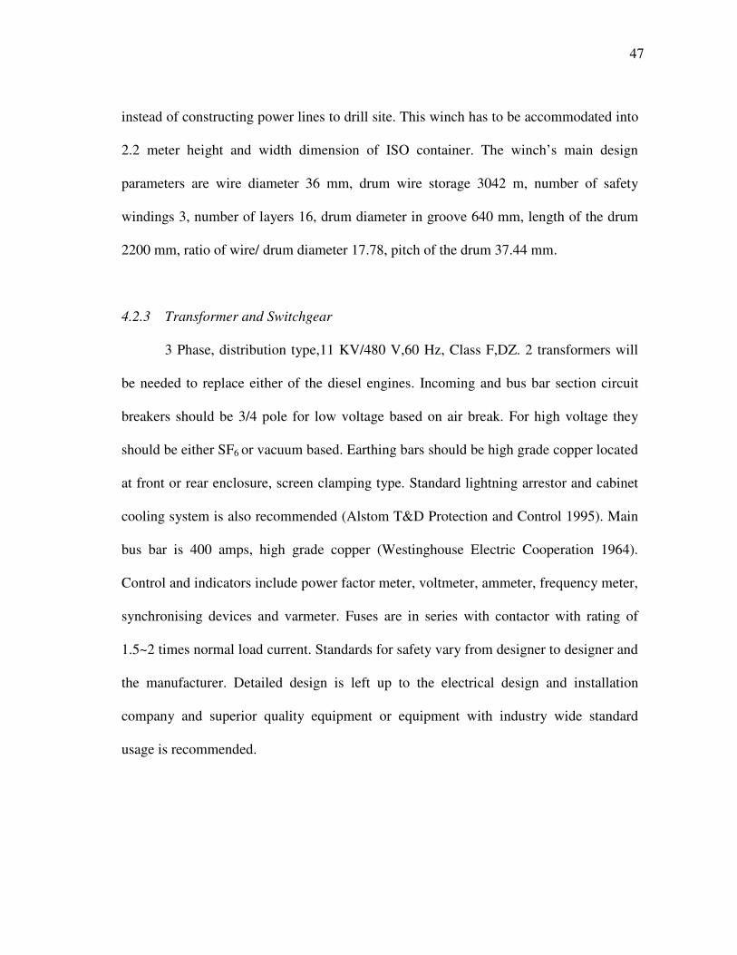
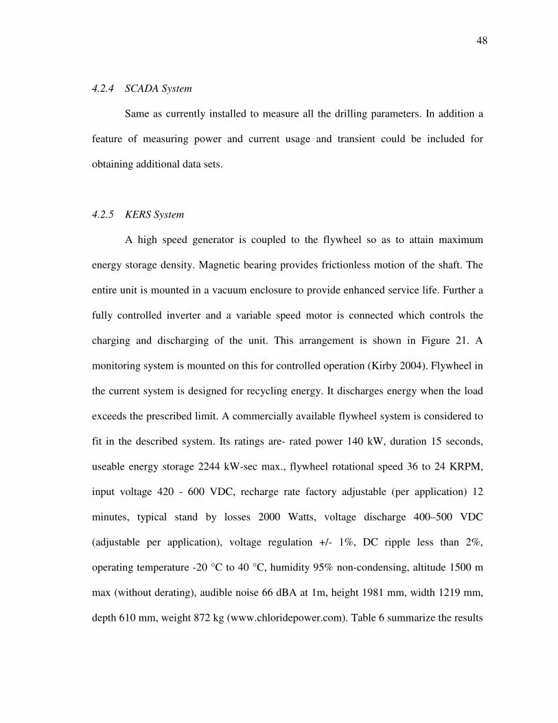
4.2.5 KERS System
A high speed generator is coupled to the flywheel so as to attain maximum
energy storage density. Magnetic bearing provides frictionless motion of the shaft. The
entire unit is mounted in a vacuum enclosure to provide enhanced service life. Further a
fully controlled inverter and a variable speed motor is connected which controls the
charging and discharging of the unit. This arrangement is shown in Figure 21. A
monitoring system is mounted on this for controlled operation (Kirby 2004). Flywheel in
the current system is designed for recycling energy. It discharges energy when the load
exceeds the prescribed limit. A commercially available flywheel system is considered to
fit in the described system. Its ratings are- rated power 140 kW, duration 15 seconds,
useable energy storage 2244 kW-sec max., flywheel rotational speed 36 to 24 KRPM,
input voltage 420 - 600 VDC, recharge rate factory adjustable (per application) 12
minutes, typical stand by losses 2000 Watts, voltage discharge 400–500 VDC
(adjustable per application), voltage regulation +/- 1%, DC ripple less than 2%,
operating temperature -20 °C to 40 °C, humidity 95% non-condensing, altitude 1500 m
max (without derating), audible noise 66 dBA at 1m, height 1981 mm, width 1219 mm,
depth 610 mm, weight 872 kg (www.chloridepower.com). Table 6 summarize the results
49�
from data processing and explore the possibility of this flywheel unit for being
successfully implemented in the overall system. Other modern high speed flywheel units
can also be incorporated considering size constraint of 20 ft ISO container and safety
regulations. This investigation is primarily concerned with proving that flywheel unit
can be successfully implemented for peak shaving in drilling rigs.
Figure 22 – KERS system positioning and operation
50�
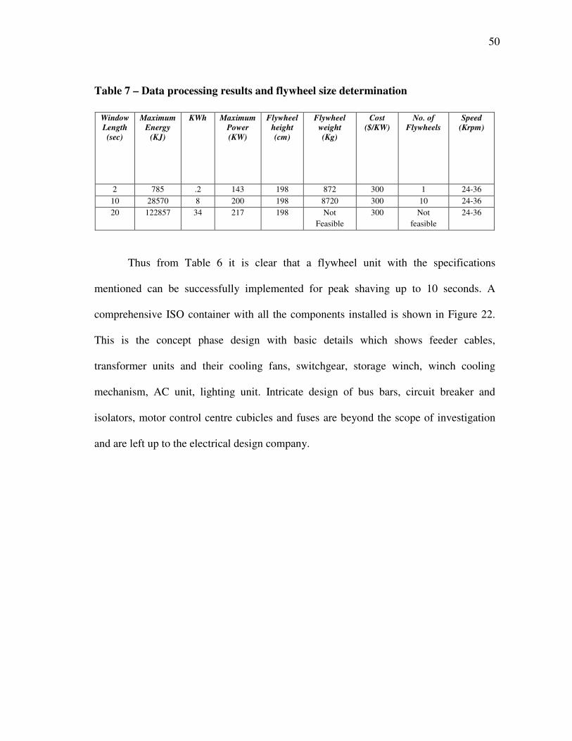
Table 7 – Data processing results and flywheel size determination
Thus from Table 6 it is clear that a flywheel unit with the specifications
mentioned can be successfully implemented for peak shaving up to 10 seconds. A
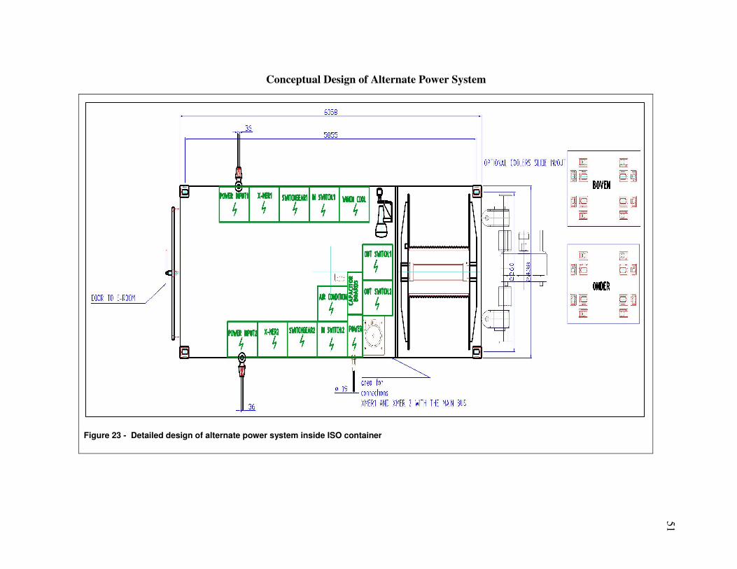
comprehensive ISO container with all the components installed is shown in Figure 22.
This is the concept phase design with basic details which shows feeder cables,
transformer units and their cooling fans, switchgear, storage winch, winch cooling
mechanism, AC unit, lighting unit. Intricate design of bus bars, circuit breaker and
isolators, motor control centre cubicles and fuses are beyond the scope of investigation
and are left up to the electrical design company.
Window Length (sec)
Maximum Energy
(KJ)
KWh Maximum Power (KW)
Flywheel height (cm)
Flywheel weight (Kg)
Cost ($/KW)
No. of Flywheels
Speed (Krpm)
2 785 .2 143 198 872 300 1 24-36 10 28570 8 200 198 8720 300 10 24-36 20 122857 34 217 198 Not
Feasible 300 Not
feasible 24-36
51
Figure 23 - Detailed design of alternate power system inside ISO container
Conceptual Design of Alternate Power System
52
5. CONCLUSION
5.1 Results
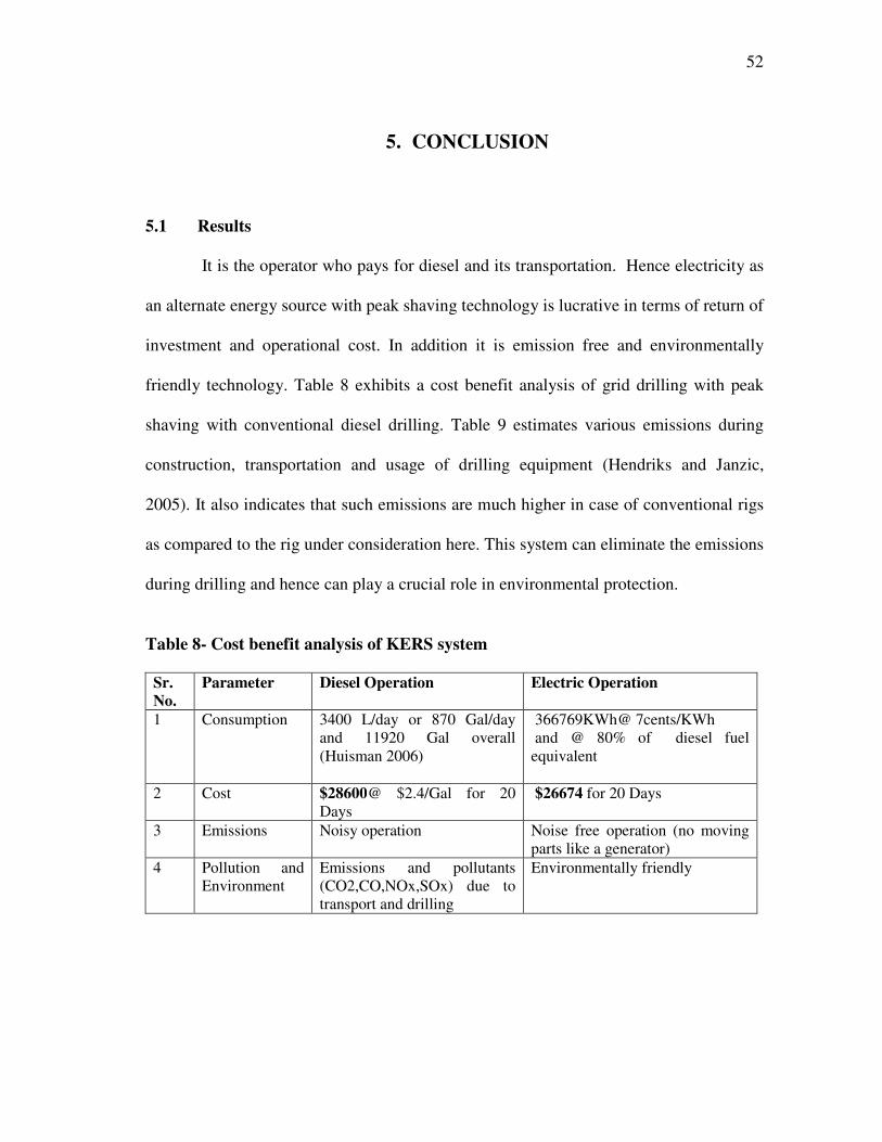
It is the operator who pays for diesel and its transportation. Hence electricity as
an alternate energy source with peak shaving technology is lucrative in terms of return of
investment and operational cost. In addition it is emission free and environmentally
friendly technology. Table 8 exhibits a cost benefit analysis of grid drilling with peak
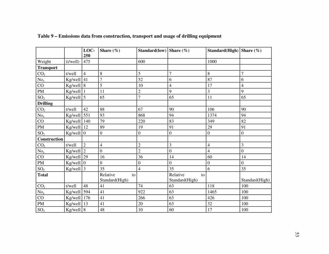
shaving with conventional diesel drilling. Table 9 estimates various emissions during
construction, transportation and usage of drilling equipment (Hendriks and Janzic,
2005). It also indicates that such emissions are much higher in case of conventional rigs
as compared to the rig under consideration here. This system can eliminate the emissions
during drilling and hence can play a crucial role in environmental protection.
Table 8- Cost benefit analysis of KERS system
Sr. No.
Parameter Diesel Operation Electric Operation
1 Consumption 3400 L/day or 870 Gal/day and 11920 Gal overall (Huisman 2006)
366769KWh@ 7cents/KWh and @ 80% of diesel fuel equivalent
2 Cost $28600@ $2.4/Gal for 20 Days
$26674 for 20 Days
3 Emissions Noisy operation Noise free operation (no moving parts like a generator)
4 Pollution and Environment
Emissions and pollutants (CO2,CO,NOx,SOx) due to transport and drilling
Environmentally friendly
53�
LOC-250
Share (%) Standard(low) Share (%) Standard(High) Share (%)
Weight (t/well) 475 600 1000 Transport CO2 t/well 4 8 5 7 8 7 Nox Kg/well 41 7 52 6 87 6 CO Kg/well 8 5 10 4 17 4 PM Kg/well 1 11 2 9 3 9 SO2 Kg/well 5 65 7 65 11 65 Drilling CO2 t/well 42 88 67 90 106 90 Nox Kg/well 551 93 868 94 1374 94 CO Kg/well 140 79 220 83 349 82 PM Kg/well 12 89 19 91 29 91 SO2 Kg/well 0 0 0 0 0 0 Construction CO2 t/well 2 4 2 3 4 3 Nox Kg/well 2 0 2 0 4 0 CO Kg/well 29 16 36 14 60 14 PM Kg/well 0 0 0 0 0 0 SO2 Kg/well 3 35 4 35 6 35 Total Relative to
Standard(High) Relative to
Standard(High)
Standard(High) CO2 t/well 48 41 74 63 118 100 Nox Kg/well 594 41 922 63 1465 100 CO Kg/well 176 41 266 63 426 100 PM Kg/well 13 41 20 63 32 100 SO2 Kg/well 8 48 10 60 17 100
Table 9 – Emissions data from construction, transport and usage of drilling equipment
54�
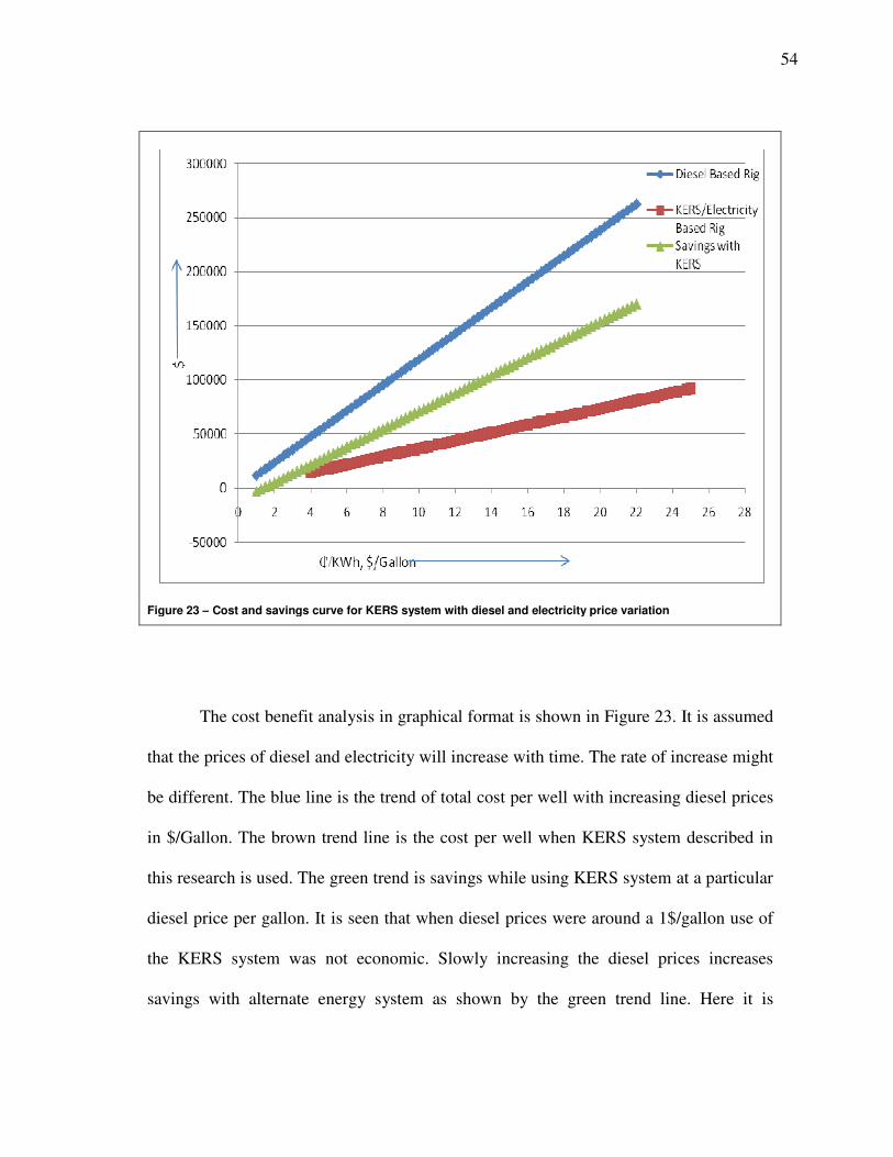
Figure 23 – Cost and savings curve for KERS system with diesel and electricity price variation
The cost benefit analysis in graphical format is shown in Figure 23. It is assumed
that the prices of diesel and electricity will increase with time. The rate of increase might
be different. The blue line is the trend of total cost per well with increasing diesel prices
in $/Gallon. The brown trend line is the cost per well when KERS system described in
this research is used. The green trend is savings while using KERS system at a particular
diesel price per gallon. It is seen that when diesel prices were around a 1$/gallon use of
the KERS system was not economic. Slowly increasing the diesel prices increases
savings with alternate energy system as shown by the green trend line. Here it is
55�
assumed that the fuel consumption of a particular rig, LOC-250 in this case, will be more
or less the same for an average well with average depth of 8000ft.
5.2 Inferences
Hence we come up with following conclusions from this research project:
• The power consumption of casing while drilling rigs, LOC-250 and LOC-400 is
much lesser than conventional rigs.
• It is possible to connect these rigs to electrical grid. It is also possible to install a
KERS system which can successfully provide peak shaving and reduce the
transient power peaks.
• Such an alternate power system can be made mobile with no special freight
requirements.
• LOC 400 being an electrically driven system can be easily connected to a power
grid within 2 miles of radius.
• It is possible to eliminate all the drilling emissions with this KERS system
operating with electrical grid.
• Savings after installing this system increase linearly with increasing cost of
diesel.
• The rig with both alternate power system and conventional diesel engines
consumes lesser diesel as compared to the same rig with standalone diesel
engines. This is true for an average well duration of 20 days and average well
depth of 8000 ft.
56�
5.3 Future Work
Following investigation can also be conducted in future:
• Analysis of the regenerative power by LOC-400 and losses.
• Detailed design of switchgear and their single line diagrams with rating of fuses
and circuit breakers.
• Replacement of flywheel by super capacitor units and redo the peak shaving
design once super capacitors are successfully tested.
• Cost quotation and return of investment of switchgear components, flywheel
unit, installation and maintenance.
• Design of cooling system for storage winch.
• Study of Environmental regulations in order to lay out high voltage cable on
ground.
• Simulation of the circuit design.
• Safety guidelines for operation of KERS based rig power system.
• Interviews with utility companies regarding surcharges and special regulations
which vary with state.
• Calculation of power factor of the rig.
• Lab testing of KERS coupled diesel engines to estimate exact fuel savings.

57�
NOMENCLATURE
AC Alternating Current
Amps Amperes
�C Degree Centigrade
Cm Centi Meters
CO2 Carbon dioxide
DC Direct Current
dBA Decibels
ft Feet
gpm Gallons Per Minute
Hz Hertz
ISO International Organization of Standards
KERS Kinetic Energy Recovery and Storage
kG Kilo Grams
kJ Kilo Joules
kRPM Kilo Rotations Per Minute
kV Kilo Volts
kW Kilo Watts
kWh Kilo Watt Hour
l Litres
LOC 250 Land Offshore Containerized (with hook load of 250 Tonnes)
58�
MATLAB Mathematics Laboratory
mm Milli Meter
MVA Mega Electron Volt
NOx Family of Nitrogen Oxides
SCADA Supervisory Control And Data Acquisition System
SF6 Sulphur Hexa Fluoride
SOx Family of Sulphur Oxides
V Volts
XLPE Cross Linked Polyethylene
59�
REFERENCES Brobeck, W.M. and Associates. Conceptual Design of a Flywheel Energy Storage System. Sandia Laboratories, Contract No.DE-AC04-76DP00789, United States Department of Energy, Washington DC (Nov 1979). Commercial flywheel unit ratings, Chloride Power website. 2008: www.chloridepower.com. (Accessed on Jul 2008). EG&G Services, Parsons Inc. Fuel Cell Handbook, Fifth Edition, Science Applications International Corporation, Contract No. DE-AM26-99FT40575, United States Department of Energy, Washington DC. (Oct 2000). Electrical Transmission and Distribution Reference Book, eighth edition, 1964. East Pittsburg, PA: Central Station Engineers of the Westinghouse Electric Cooperation. Electricity prices, Electricity Bid website. 2008: www.electricitybid.com. (Accessed on Jan 2008). Fink D.G., Beaty, H.W. 1987. Standard Handbook for Electrical Engineers, NY: McGraw Hill Book Company Inc. Flywheel applications, Beacon Power website. 2008: www.beaconpower.com. (Accessed on Aug 2008). Hendriks, K., Janzic, R. 2005. Environmental impact of standard oil drilling installations versus LOC 250. Ecofys Report for Huisman US, Ref: A04-10050. Huisman Special Lifting Equipment B.V. 2005. LOC250 Casing Drilling Manual Version 1.0. Schiedam, Netherlands: Huisman. Huisman Special Lifting Equipment B.V. 2007. Technical Specification LOC400: Husiman Itrec. Huisman Special Lifting Equipment B.V. 2006 ,User Manual for Containerized Drilling Unit, System Description, Specifications, Operation and Maintenance Volume 1, A04-45000, Schiedam, Netherlands: Huisman. Kirby, Brendon, PE. 2004. Frequency Regulations Basics and Trends. Power System Research Program Oak Ridge National Laboratory, Oak Ridge, Contract No.DE-AC05-00OR22725, US D.O.E, Washington DC. (Jul. 2004). McAllister, D. 1987. Electrical Cables Handbook. BICC Power Cables Ltd, London,
60�
UK: Granada Publishing Ltd. Nichols, D.K, Eckroad, S., 2003. Utility Scale Application of Sodium Sulfur Battery. Battcon, www.battcon.com/PapersFinal2003/NicholsPaperFINAL2003.pdf. Downloaded January 2009. Protective Relay Application Guide, third edition, 1995. Stafford UK: Alstom T&D Protection and Control Ltd. Rogers, J.D., 2006, Report on Assessment of Technologies for Environmental Friendly Drilling Project: Land Based Operations, draft 3, version 2, Houston Advance Research Center. Rojas, A. 2004. Flywheel Energy Matrix Systems – Today’s Technology, Tomorrow’s Energy Storage Solution. Conference Proc., IEEE Power Engineering Society General Meeting, Denver, CO. Romo, L., Solis,O., Matthews,J., Qin, D. 2007, Fuel Saving Flywheel Technology for Rubber Tired Gantry Cranes in World Ports: Reducing Fuel Consumption through Flywheel Energy Storage System, Final Report, VYOCON ENERGY, CA (2007). Ruddell, Alan. 2003. Storage Technology Report ST6: Flywheel.Deliverable_5_030617_CCLRC-RAL, CCLRC-Rutherford Appleton Laboratory, Didcot, UK. Solar calculator, FindSolar website. 2009: www.findsolar.com. (Accessed on Mar 2009).
Solar cells, US Department of Energy website. 2009: www.eere.energy.gov. (Accessed on Feb 2009). Tamyurek, B., Nichols, D.K., Demirci, O. 2003. Sodium Sulfur Battery Applications. Conf Proc., IEEE Power Engineering Society General Meeting, Volume 4, OH. Walsh, B., Wichert, R., 2008. Fuel Cell Technology. www.wbdg.org. (Accessed on May 2008).
61�
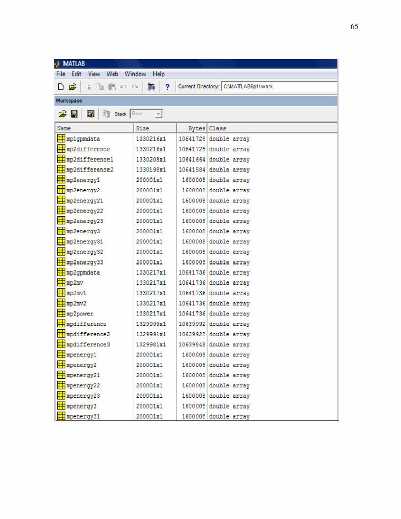
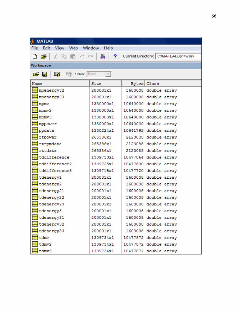
APPENDIX A
VARIABLE DESCRIPTION FOR MATLAB CODE AND
SCREENSHOTS
62�
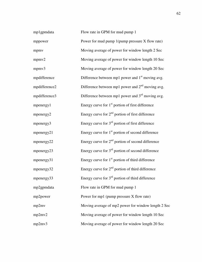
mp1gpmdata Flow rate in GPM for mud pump 1
mppower Power for mud pump 1(pump pressure X flow rate)
mpmv Moving average of power for window length 2 Sec
mpmv2 Moving average of power for window length 10 Sec
mpmv3 Moving average of power for window length 20 Sec
mpdifference Difference between mp1 power and 1st moving avg.
mpdifference2 Difference between mp1 power and 2nd moving avg.
mpdifference3 Difference between mp1 power and 3rd moving avg.
mpenergy1 Energy curve for 1st portion of first difference
mpenergy2 Energy curve for 2nd portion of first difference
mpenergy3 Energy curve for 3rd portion of first difference
mpenergy21 Energy curve for 1st portion of second difference
mpenergy22 Energy curve for 2nd portion of second difference
mpenergy23 Energy curve for 3rd portion of second difference
mpenergy31 Energy curve for 1st portion of third difference
mpenergy32 Energy curve for 2nd portion of third difference
mpenergy33 Energy curve for 3rd portion of third difference
mp2gpmdata Flow rate in GPM for mud pump 1
mp2power Power for mp1 (pump pressure X flow rate)
mp2mv Moving average of mp2 power for window length 2 Sec
mp2mv2 Moving average of power for window length 10 Sec
mp2mv3 Moving average of power for window length 20 Sec
63�
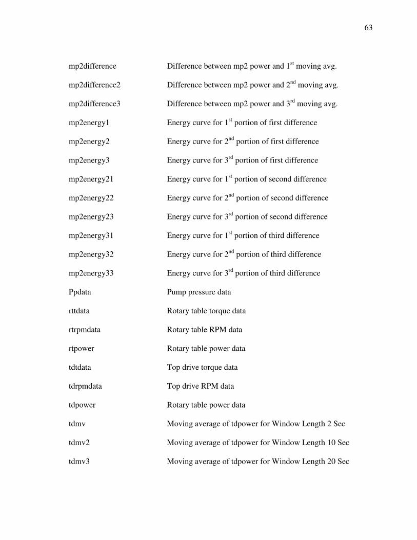
mp2difference Difference between mp2 power and 1st moving avg.
mp2difference2 Difference between mp2 power and 2nd moving avg.
mp2difference3 Difference between mp2 power and 3rd moving avg.
mp2energy1 Energy curve for 1st portion of first difference
mp2energy2 Energy curve for 2nd portion of first difference
mp2energy3 Energy curve for 3rd portion of first difference
mp2energy21 Energy curve for 1st portion of second difference
mp2energy22 Energy curve for 2nd portion of second difference
mp2energy23 Energy curve for 3rd portion of second difference
mp2energy31 Energy curve for 1st portion of third difference
mp2energy32 Energy curve for 2nd portion of third difference
mp2energy33 Energy curve for 3rd portion of third difference
Ppdata Pump pressure data
rttdata Rotary table torque data
rtrpmdata Rotary table RPM data
rtpower Rotary table power data
tdtdata Top drive torque data
tdrpmdata Top drive RPM data
tdpower Rotary table power data
tdmv Moving average of tdpower for Window Length 2 Sec
tdmv2 Moving average of tdpower for Window Length 10 Sec
tdmv3 Moving average of tdpower for Window Length 20 Sec
64�
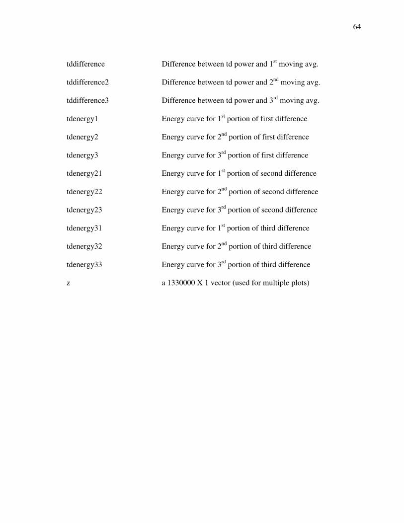
tddifference Difference between td power and 1st moving avg.
tddifference2 Difference between td power and 2nd moving avg.
tddifference3 Difference between td power and 3rd moving avg.
tdenergy1 Energy curve for 1st portion of first difference
tdenergy2 Energy curve for 2nd portion of first difference
tdenergy3 Energy curve for 3rd portion of first difference
tdenergy21 Energy curve for 1st portion of second difference
tdenergy22 Energy curve for 2nd portion of second difference
tdenergy23 Energy curve for 3rd portion of second difference
tdenergy31 Energy curve for 1st portion of third difference
tdenergy32 Energy curve for 2nd portion of third difference
tdenergy33 Energy curve for 3rd portion of third difference
z a 1330000 X 1 vector (used for multiple plots)
65�
66�

67�
APPENDIX B
CONVERSION FACTORS
68�
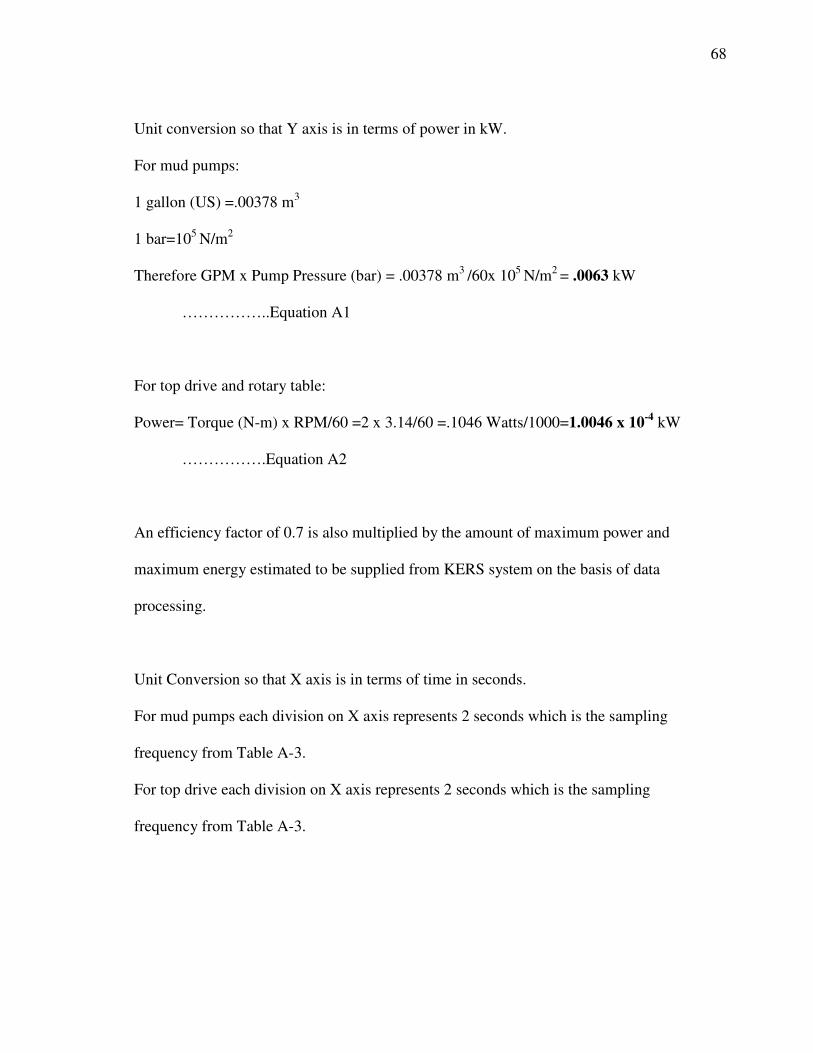
Unit conversion so that Y axis is in terms of power in kW.
For mud pumps:
1 gallon (US) =.00378 m3
1 bar=105 N/m2
Therefore GPM x Pump Pressure (bar) = .00378 m3 /60x 105 N/m2 = .0063 kW
……………..Equation A1
For top drive and rotary table:
Power= Torque (N-m) x RPM/60 =2 x 3.14/60 =.1046 Watts/1000=1.0046 x 10-4 kW
…………….Equation A2
An efficiency factor of 0.7 is also multiplied by the amount of maximum power and
maximum energy estimated to be supplied from KERS system on the basis of data
processing.
Unit Conversion so that X axis is in terms of time in seconds.
For mud pumps each division on X axis represents 2 seconds which is the sampling
frequency from Table A-3.
For top drive each division on X axis represents 2 seconds which is the sampling
frequency from Table A-3.

69�
APPENDIX C
RESULTS DATA
70�
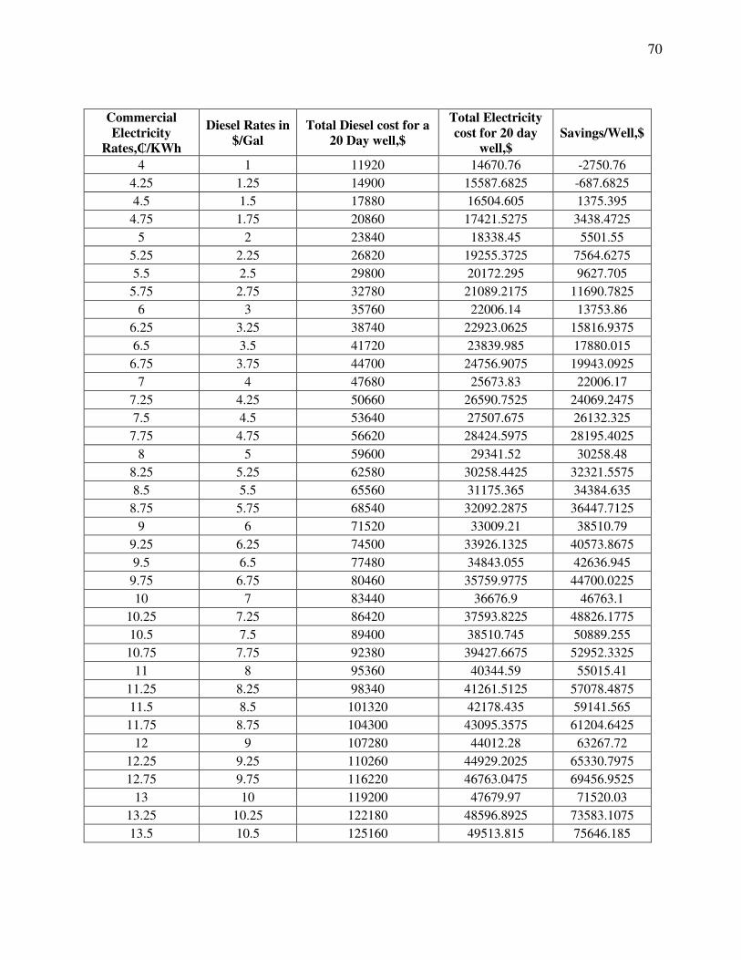
Commercial Electricity
Rates,�/KWh
Diesel Rates in $/Gal
Total Diesel cost for a 20 Day well,$
Total Electricity cost for 20 day
well,$ Savings/Well,$
4 1 11920 14670.76 -2750.76 4.25 1.25 14900 15587.6825 -687.6825 4.5 1.5 17880 16504.605 1375.395
4.75 1.75 20860 17421.5275 3438.4725 5 2 23840 18338.45 5501.55
5.25 2.25 26820 19255.3725 7564.6275 5.5 2.5 29800 20172.295 9627.705
5.75 2.75 32780 21089.2175 11690.7825 6 3 35760 22006.14 13753.86
6.25 3.25 38740 22923.0625 15816.9375 6.5 3.5 41720 23839.985 17880.015
6.75 3.75 44700 24756.9075 19943.0925 7 4 47680 25673.83 22006.17
7.25 4.25 50660 26590.7525 24069.2475 7.5 4.5 53640 27507.675 26132.325
7.75 4.75 56620 28424.5975 28195.4025 8 5 59600 29341.52 30258.48
8.25 5.25 62580 30258.4425 32321.5575 8.5 5.5 65560 31175.365 34384.635
8.75 5.75 68540 32092.2875 36447.7125 9 6 71520 33009.21 38510.79
9.25 6.25 74500 33926.1325 40573.8675 9.5 6.5 77480 34843.055 42636.945
9.75 6.75 80460 35759.9775 44700.0225 10 7 83440 36676.9 46763.1
10.25 7.25 86420 37593.8225 48826.1775 10.5 7.5 89400 38510.745 50889.255
10.75 7.75 92380 39427.6675 52952.3325 11 8 95360 40344.59 55015.41
11.25 8.25 98340 41261.5125 57078.4875 11.5 8.5 101320 42178.435 59141.565
11.75 8.75 104300 43095.3575 61204.6425 12 9 107280 44012.28 63267.72
12.25 9.25 110260 44929.2025 65330.7975 12.75 9.75 116220 46763.0475 69456.9525
13 10 119200 47679.97 71520.03 13.25 10.25 122180 48596.8925 73583.1075 13.5 10.5 125160 49513.815 75646.185
71�
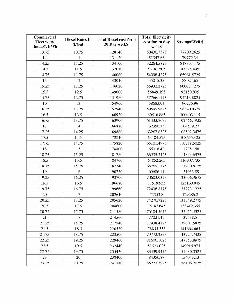
Commercial Electricity
Rates,�/KWh
Diesel Rates in $/Gal
Total Diesel cost for a 20 Day well,$
Total Electricity cost for 20 day
well,$ Savings/Well,$
13.75 10.75 128140 50430.7375 77709.2625 14 11 131120 51347.66 79772.34
14.25 11.25 134100 52264.5825 81835.4175 14.5 11.5 137080 53181.505 83898.495
14.75 11.75 140060 54098.4275 85961.5725 15 12 143040 55015.35 88024.65
15.25 12.25 146020 55932.2725 90087.7275 15.5 12.5 149000 56849.195 92150.805
15.75 12.75 151980 57766.1175 94213.8825 16 13 154960 58683.04 96276.96
16.25 13.25 157940 59599.9625 98340.0375 16.5 13.5 160920 60516.885 100403.115
16.75 13.75 163900 61433.8075 102466.1925 17 14 166880 62350.73 104529.27
17.25 14.25 169860 63267.6525 106592.3475 17.5 14.5 172840 64184.575 108655.425
17.75 14.75 175820 65101.4975 110718.5025 18 15 178800 66018.42 112781.58
18.25 15.25 181780 66935.3425 114844.6575 18.5 15.5 184760 67852.265 116907.735
18.75 15.75 187740 68769.1875 118970.8125 19 16 190720 69686.11 121033.89
19.25 16.25 193700 70603.0325 123096.9675 19.5 16.5 196680 71519.955 125160.045
19.75 16.75 199660 72436.8775 127223.1225 20 17 202640 73353.8 129286.2
20.25 17.25 205620 74270.7225 131349.2775 20.5 17.5 208600 75187.645 133412.355
20.75 17.75 211580 76104.5675 135475.4325 21 18 214560 77021.49 137538.51
21.25 18.25 217540 77938.4125 139601.5875 21.5 18.5 220520 78855.335 141664.665
21.75 18.75 223500 79772.2575 143727.7425 22.25 19.25 229460 81606.1025 147853.8975 22.5 19.5 232440 82523.025 149916.975
22.75 19.75 235420 83439.9475 151980.0525 23 20 238400 84356.87 154043.13
23.25 20.25 241380 85273.7925 156106.2075
72�
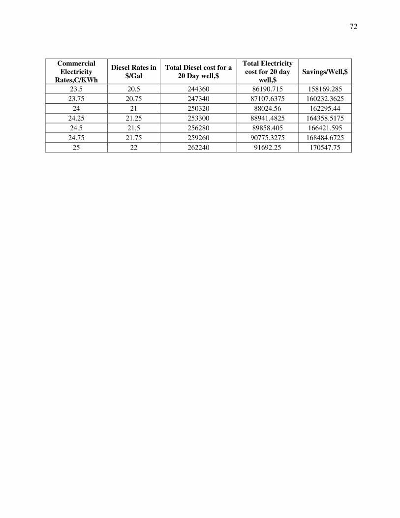
Commercial Electricity
Rates,�/KWh
Diesel Rates in $/Gal
Total Diesel cost for a 20 Day well,$
Total Electricity cost for 20 day
well,$ Savings/Well,$
23.5 20.5 244360 86190.715 158169.285 23.75 20.75 247340 87107.6375 160232.3625
24 21 250320 88024.56 162295.44 24.25 21.25 253300 88941.4825 164358.5175 24.5 21.5 256280 89858.405 166421.595
24.75 21.75 259260 90775.3275 168484.6725 25 22 262240 91692.25 170547.75

73�
APPENDIX D
OTHER IMPORTANT MATLAB PLOTS
74�
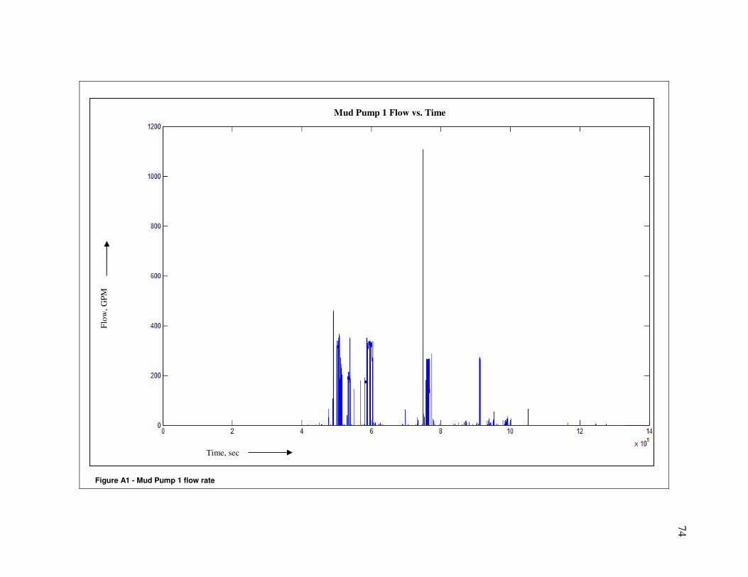
Figure A1 - Mud Pump 1 flow rate
Time, sec
Flow
, GPM
Mud Pump 1 Flow vs. Time
75�
Figure A2 - Mud Pump 1 instantaneous power (blue) and moving average (green) of window length of 10 seconds
Time, sec
Pow
er, k
W
Mud Pump 1 Moving Average Power Curve for 10 sec vs. Time
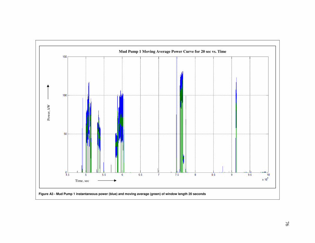
76�
Figure A3 - Mud Pump 1 instantaneous power (blue) and moving average (green) of window length 20 seconds
Time, sec
Pow
er, k
W
Mud Pump 1 Moving Average Power Curve for 20 sec vs. Time
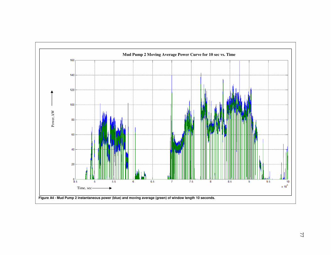
77�
Figure A4 - Mud Pump 2 instantaneous power (blue) and moving average (green) of window length 10 seconds.
Pow
er, k
W
Time, sec
Mud Pump 2 Moving Average Power Curve for 10 sec vs. Time
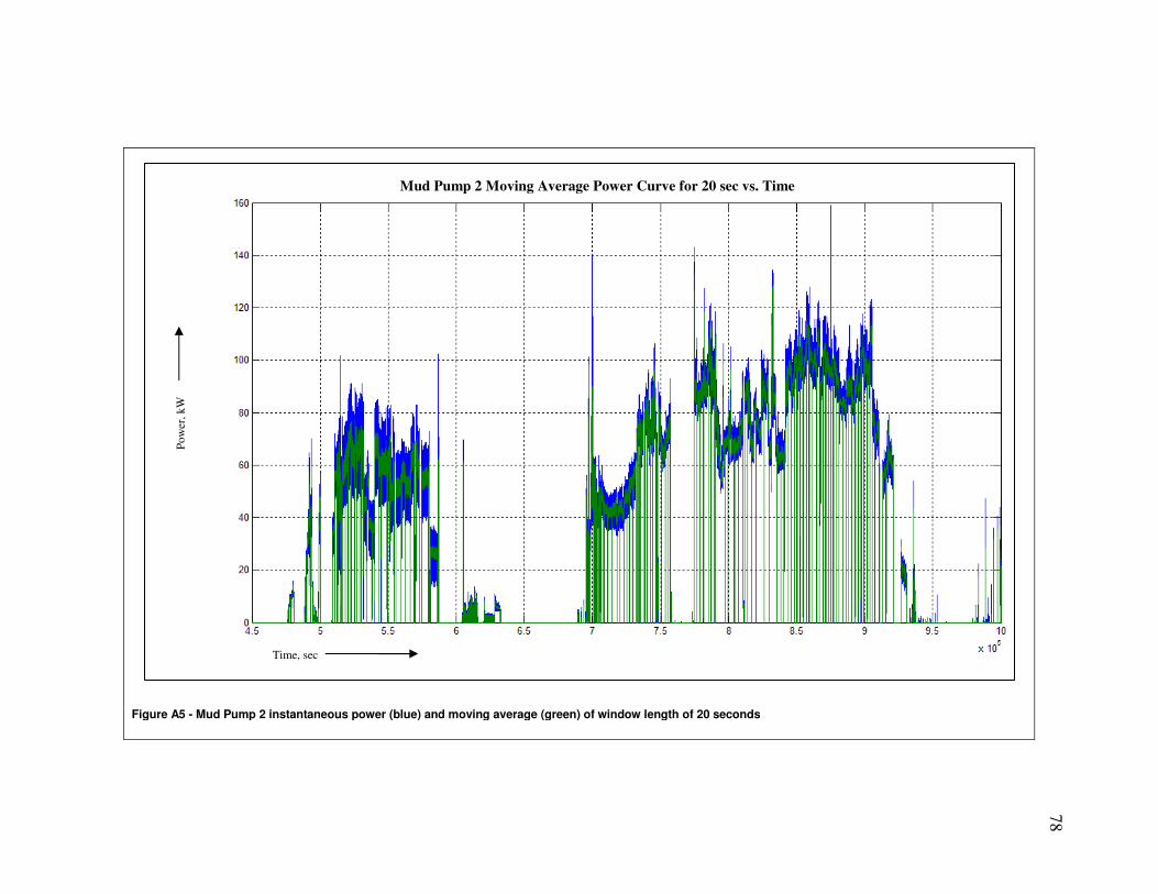
78�
Figure A5 - Mud Pump 2 instantaneous power (blue) and moving average (green) of window length of 20 seconds
Time, sec
Pow
er, k
W
Mud Pump 2 Moving Average Power Curve for 20 sec vs. Time
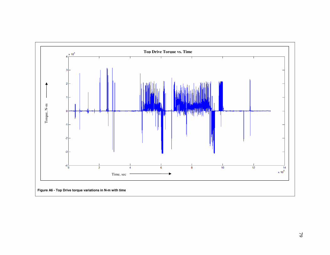
79�
Figure A6 - Top Drive torque variations in N-m with time
Time, sec
Tor
que,
N-m
Top Drive Torque vs. Time
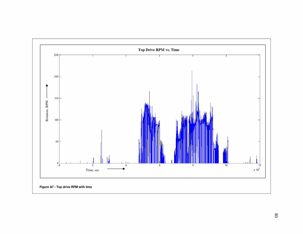
80�
Figure A7 - Top drive RPM with time
Time, sec
Mud Pump 2 Moving Average Power Curve for 20 sec Vs. Time R
otat
ion,
RPM
Time, sec
Top Drive RPM vs. Time
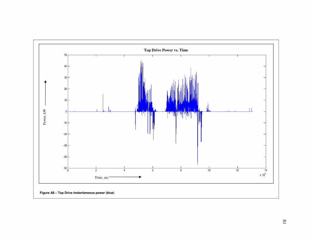
81�
Figure A8 – Top Drive instantaneous power (blue)
Time, sec
Mud Pump 2 Moving Average Power Curve for 20 sec Vs. Time
Time, sec
Top Drive RPM Vs. Time
Pow
er, k
W
Time, sec
Top Drive Power vs. Time
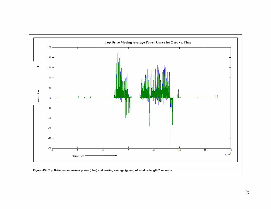
82�
Figure A9 - Top Drive instantaneous power (blue) and moving average (green) of window length 2 seconds
Time, sec
Mud Pump 2 Moving Average Power Curve for 20 sec Vs. Time
Time, sec
Top Drive RPM Vs. Time
Time, sec
Top Drive Power Vs. Time
Pow
er, k
W
Time, sec
Top Drive Moving Average Power Curve for 2 sec vs. Time
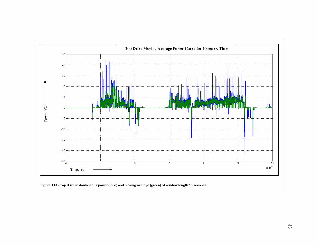
83�
Figure A10 - Top drive instantaneous power (blue) and moving average (green) of window length 10 seconds
Mud Pump 2 Moving Average Power Curve for 20 sec Vs. Time Top Drive RPM Vs. Time Top Drive Power Vs. Time Top Drive Moving Average Power Curve for 2 sec Vs. Time Po
wer
, kW
Time, sec
Top Drive Moving Average Power Curve for 10 sec vs. Time
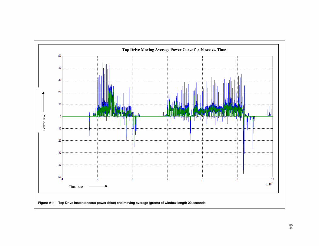
84�
Figure A11 – Top Drive instantaneous power (blue) and moving average (green) of window length 20 seconds
Mud Pump 2 Moving Average Power Curve for 20 sec Vs. Time Top Drive RPM Vs. Time Top Drive Power Vs. Time Top Drive Moving Average Power Curve for 2 sec Vs. Time
Time, sec
Top Drive Moving Average Power Curve for 10 sec Vs. Time
Time, sec
Pow
er, k
W
Top Drive Moving Average Power Curve for 20 sec vs. Time
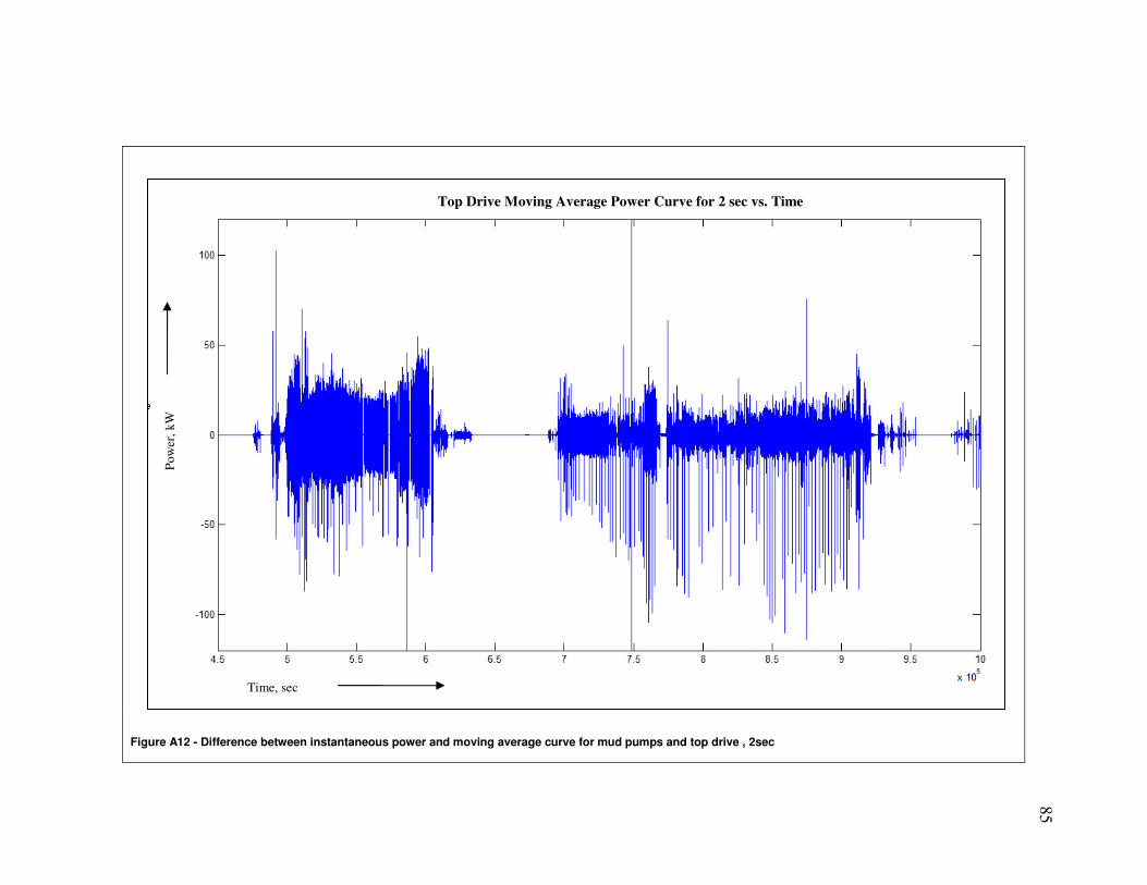
85�
Figure A12 - Difference between instantaneous power and moving average curve for mud pumps and top drive , 2sec
Mud Pump 2 Moving Average Power Curve for 20 sec Vs. Time Top Drive RPM Vs. Time Top Drive Power Vs. Time
Time, sec
Top Drive Moving Average Power Curve for 10 sec vs. Time
Time, sec
Pow
er, k
W
Top Drive Moving Average Power Curve for 20 sec Vs. Time
Pow
er, k
W
Time, sec
Top Drive Moving Average Power Curve for 2 sec vs. Time
Pow
er, k
W
Time, sec
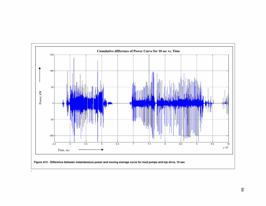
86�
Figure A13 - Difference between instantaneous power and moving average curve for mud pumps and top drive, 10 sec
.
Mud Pump 2 Moving Average Power Curve for 20 sec Vs. Time Top Drive RPM Vs. Time Top Drive Power Vs. Time Top Drive Moving Average Power Curve for 2 sec Vs. Time
Time, sec
Top Drive Moving Average Power Curve for 10 sec Vs. Time
Pow
er, k
W
Cumulative difference of Power Curve for 10 sec vs. Time
Time, sec
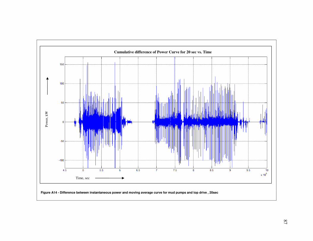
87�
Figure A14 - Difference between instantaneous power and moving average curve for mud pumps and top drive , 20sec
Pow
er, k
W
Cumulative difference of Power Curve for 20 sec vs. Time
Time, sec
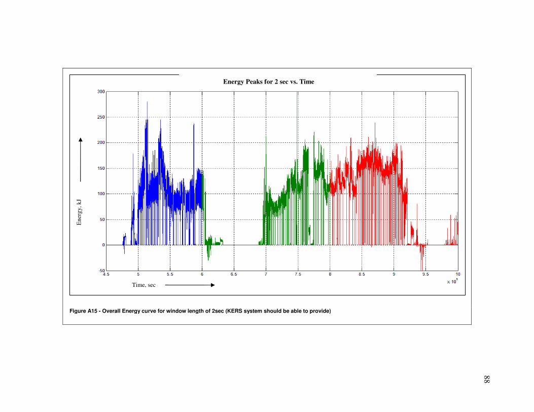
88�
Figure A15 - Overall Energy curve for window length of 2sec (KERS system should be able to provide)
Ene
rgy,
kJ
Energy Peaks for 2 sec vs. Time
Time, sec
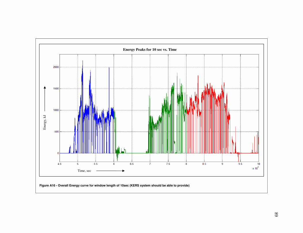
89�
Figure A16 - Overall Energy curve for window length of 10sec (KERS system should be able to provide)
Time, sec
Ene
rgy,
kJ
Time, sec
Energy Peaks for 10 sec vs. Time
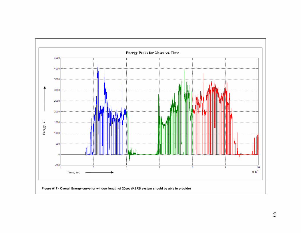
90�
Figure A17 - Overall Energy curve for window length of 20sec (KERS system should be able to provide)
Time, sec
Time, sec
Ene
rgy,
kJ
Time, sec
Energy Peaks for 20 sec vs. Time
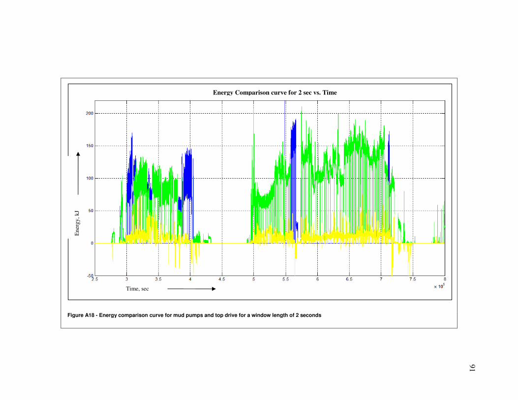
91�
Figure A18 - Energy comparison curve for mud pumps and top drive for a window length of 2 seconds
Time, sec
Energy Peaks for 20 sec vs. Time
Time, sec
Ene
rgy,
kJ
Energy Comparison curve for 2 sec vs. Time
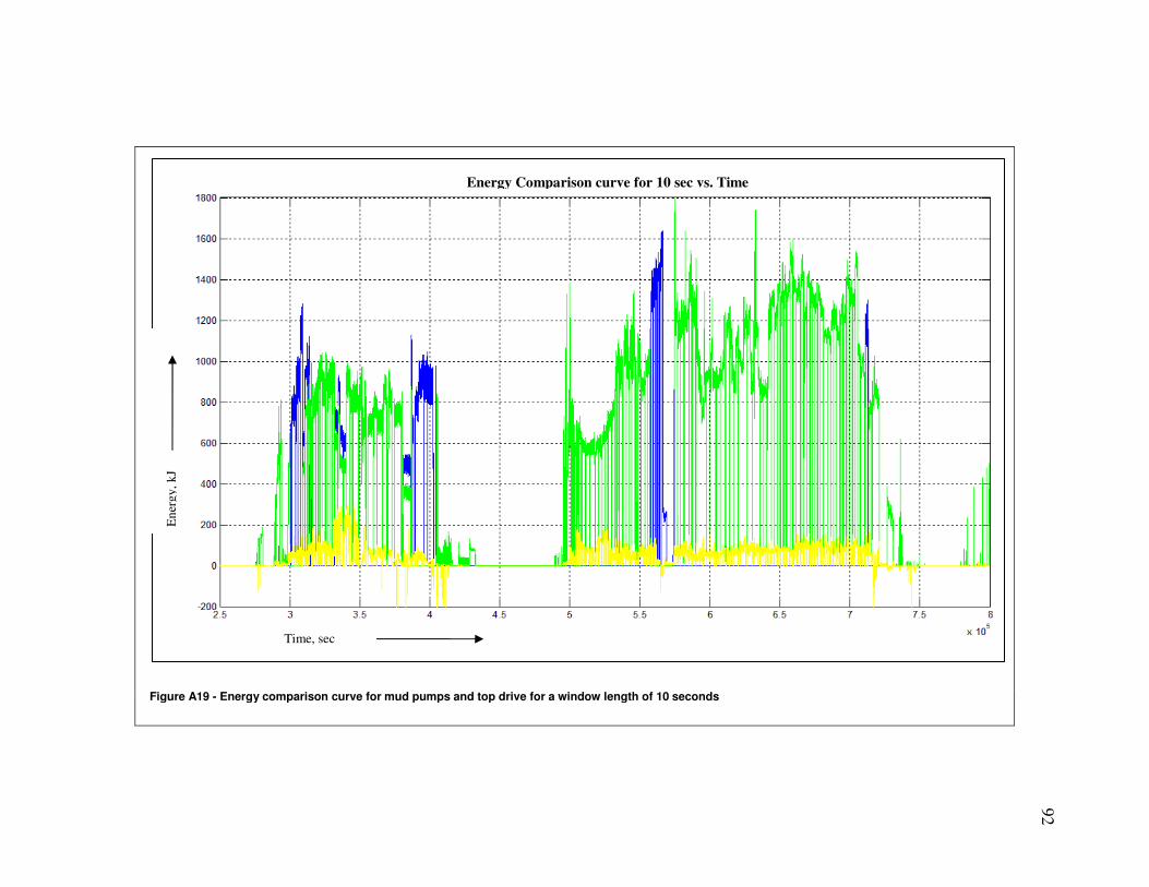
92�
Figure A19 - Energy comparison curve for mud pumps and top drive for a window length of 10 seconds
Time, sec
Energy Peaks for 20 sec vs. Time
Time, sec
Energy Comparison curve for 2 sec vs. Time E
nerg
y, k
J Energy Comparison curve for 10 sec vs. Time
Time, sec
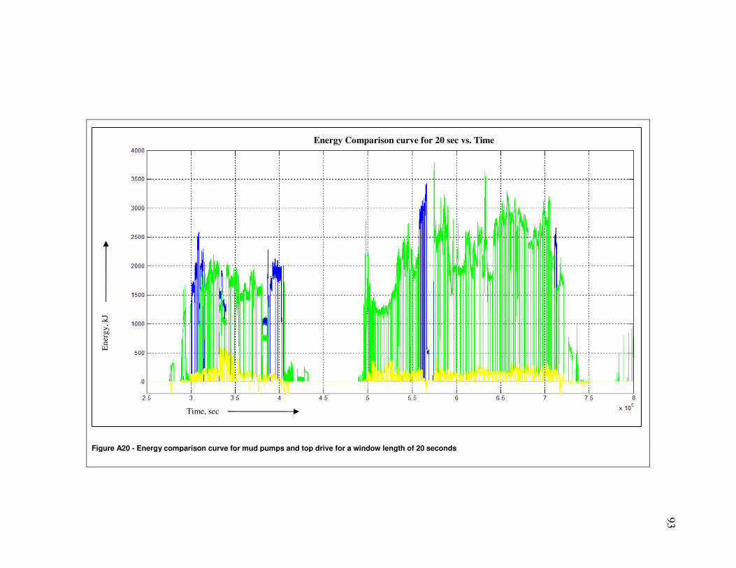
93�
Figure A20 - Energy comparison curve for mud pumps and top drive for a window length of 20 seconds
Time, sec
Energy Peaks for 20 sec vs. Time
Time, sec
Energy Comparison curve for 2 sec vs. Time Energy Comparison curve for 10 sec vs. Time
Ene
rgy,
kJ
Time, sec
Energy Comparison curve for 20 sec vs. Time

94
VITA
Name: Ankit Verma Address: TAMU mail stop 3116, Room 710A, Department of Petroleum Engineering, Texas A&M University, College Station, TX 77843 Email Address: [email protected] Education: B.Tech., Electrical Engineering, National Institute of Technology, Bhopal, India, 2007 M.S., Petroleum Engineering, Texas A&M University, USA, 2009 Member: Society of Petroleum Engineers