This is an electronic reprint of the original article.This reprint may differ from the original in pagination and typographic detail.

Powered by TCPDF (www.tcpdf.org)

This material is protected by copyright and other intellectual property rights, and duplication or sale of all or part of any of the repository collections is not permitted, except that material may be duplicated by you for your research use or educational purposes in electronic or print form. You must obtain permission for any other use. Electronic or print copies may not be offered, whether for sale or otherwise to anyone who is not an authorised user.

Almeida, Miguel; Bioucas-Dias, J.; Vigário, R.

Separation of phase-locked sources in pseudo-real MEG data

Published in:EURASIP JOURNAL ON ADVANCES IN SIGNAL PROCESSING

DOI:10.1186/1687-6180-2013-32

Published: 01/01/2013

Document VersionPublisher's PDF, also known as Version of record

Please cite the original version:Almeida, M., Bioucas-Dias, J., & Vigário, R. (2013). Separation of phase-locked sources in pseudo-real MEGdata. EURASIP JOURNAL ON ADVANCES IN SIGNAL PROCESSING, 2013, 1-12. [32]. DOI: 10.1186/1687-6180-2013-32

Almeida et al. EURASIP Journal on Advances in Signal Processing 2013, 2013:32http://asp.eurasipjournals.com/content/2013/1/32

RESEARCH Open Access

Separation of phase-locked sources inpseudo-real MEG dataMiguel Almeida1*, Jose Bioucas-Dias1 and Ricardo Vigario2

Abstract

This article addresses the blind separation of linear mixtures of synchronous signals (i.e., signals with locked phases),which is a relevant problem, e.g., in the analysis of electrophysiological signals of the brain such as theelectroencephalogram and the magnetoencephalogram (MEG). Popular separation techniques such as independentcomponent analysis are not adequate for phase-locked signals, because such signals have strong mutualdependency. Aiming at unmixing this class of signals, we have recently introduced the independent phase analysis(IPA) algorithm, which can be used to separate synchronous sources. Here, we apply IPA to pseudo-real MEG data. Theresults show that this algorithm is able to separate phase-locked MEG sources in situations where the phase jitter (i.e.,the deviation from the perfectly synchronized case) is moderate. This represents a significant step towards performingphase-based source separation on real data.

1 IntroductionIn recent years, the interest of the scientific communityin synchrony has risen. This interest is both in its phys-ical manifestations and in the development of a theoryunifying and describing those manifestations in varioussystems such as laser beams, astrophysical objects, andbrain neurons [1].It is believed that synchrony plays a relevant role in the

way different parts of the human brain interact. For exam-ple, when humans engage in a motor task, several brainregions oscillate coherently [2,3]. Also, several pathologiessuch as autism, Alzheimer, and Parkinson are associatedwith a disruption in the synchronization profile of thebrain, whereas epilepsy is associated with an anomalousincrease in synchrony (see [4] for a review).To perform inference on the synchrony of networks

present in the brain or in other real-world systems, onemust have access to the phase dynamics of the individualoscillators (which we will call “sources”). Unfortunately, inbrain electrophysiological signals such as encephalograms(EEG) and magnetoencephalograms (MEG), and in otherreal-world situations, individual oscillator signals are notdirectly measurable, and one has only access to a super-position of the sourcesa. In fact, EEG and MEG signals

*Correspondence: malmeida@lx.it.pt1Instituto de Telecomunicacoes, Lisbon, PortugalFull list of author information is available at the end of the article

measured in one sensor contain components coming fromseveral brain regions [5]. In this case, spurious synchronymay occur, as we will illustrate later.The problem of undoing this superposition is called

blind source separation (BSS). Typically, one assumes thatthe mixing is linear and instantaneous, which is a validapproximation in brain signals [6]. One must also makesome assumptions on the sources, such as in indepen-dent component analysis (ICA) where the assumption ismutual statistical independence of the sources [7]. ICAhas seen multiple applications in EEG and MEG pro-cessing (for recent applications see, e.g., [8,9]). DifferentBSS approaches use criteria other than statistical indepen-dence, such as non-negativity of sources [10,11] or time-dependent frequency spectrum criteria [12,13]. In ourcase, independence of the sources is not a valid assump-tion, because phase-locked sources are highly mutuallydependent. Also, phase-locking is not equivalent to fre-quency coherence: in fact, two signals may have a severeoverlap between their frequency spectra but still exhibitlow or no phase synchrony at all [14]. In this article, weaddress the problem of how to separate such phase-lockedsources using a phase-specific criterion.Recently, we have presented a two-stage algorithm

called independent phase analysis (IPA) which performedvery well in noiseless simulated data [15] and with mod-erate levels of added Gaussian white noise [14]. The

© 2013 Almeida et al.; licensee Springer. This is an Open Access article distributed under the terms of the Creative CommonsAttribution License (http://creativecommons.org/licenses/by/2.0), which permits unrestricted use, distribution, and reproductionin any medium, provided the original work is properly cited.

Almeida et al. EURASIP Journal on Advances in Signal Processing 2013, 2013:32 Page 2 of 12http://asp.eurasipjournals.com/content/2013/1/32

separation algorithm we then proposed uses temporaldecorrelation separation [16] as a first step, followed bythe maximization of an objective function involving thephases of the estimated sources. In [14], we presenteda “proof-of-concept” of IPA, laying down the theoreti-cal foundations of the algorithm and applying it to a toydataset of manually generated data. However, in that arti-cle we were not concerned with the application of IPAto real-world data. In this article, we study the applica-bility of IPA to pseudo-real MEG data. These data arenot yet meant to allow inference about the human brain;however, they are generated in such a way that both thesources and the mixing process mimic what actually hap-pens in the human brain. The advantage of using suchpseudo-real data is that the true solution is known, thusallowing a quantitative assessment of the performance ofthe algorithm. We also study the robustness of IPA to thecase where the sources are not perfectly phase-locked.It should however be reinforced that the algorithm pre-sented here makes no assumptions that are specific ofbrain signals, and should work in any situation wherephase-locked sources are mixed approximately linearlyand noise levels are low.This article is organized as follows. In Section 2, we

introduce the Hilbert transform. We also introduce therethe phase locking factor (PLF), a measurement of syn-chrony which is central to the algorithm; finally, we showthat synchrony is disrupted when the sources undergoa linear mixing. Section 3 describes the IPA algorithmin detail, including illustrations using a toy dataset. InSection 4, we explain how the pseudo-real MEG dataare generated and show the results obtained by IPA onthose data. These results are discussed in Section 5 andconclusions are drawn in Section 6.

2 Background2.1 Hilbert transform: phase of a real-valued signalUsually, the signals under study are real-valued discretesignals. To obtain the phase of a real signal, one can usea complex Morlet (or Gabor) wavelet transform, whichcan be seen as a bank of bandpass filters [17]. Alterna-tively, one can use the Hilbert transform, which shouldbe applied to a locally narrowband signal or be pre-ceded by appropriate filtering [18] for the meaning ofthe phase extracted by the Hilbert transform to be clear.The two transforms have been shown to be equivalentfor the study of brain signals [19], but they may differ forother kinds of signals. In this article, we chose to use theHilbert transform. To ensure that this transform yieldsmeaningful results, we will precede its use by band-passfiltering the pseudo-real MEG sources used in this arti-cle (see Section 4.1). Note that this is a very commonpreprocessing step in the analysis of real MEG signals (cf.,[20-22]).

The discrete Hilbert transform xh(t) of a band-limiteddiscrete-time signal x(t), t ∈ Z, is given by a convolution[18]

xh(t) ≡ x(t)∗h(t), where h(t) ≡⎧⎨⎩0, for even t2π t

, for odd t.

Note that the Hilbert transform is a linear operator. TheHilbert filter h(t) is not causal and has infinite duration,which makes direct implementation of the above formulaimpossible. In practice, the Hilbert transform is usuallycomputed in the frequency domain, where the aboveconvolution becomes a product of the discrete Fouriertransforms of x(t) and h(t). A more thorough mathemat-ical explanation of this transform is given in [18,23]. Weused the Hilbert transform as implemented by MATLAB.The analytic signal of x(t), denoted by x(t), is given by

x(t) ≡ x(t) + i xh(t), where i = √−1 is the imaginaryunit. The phase of x(t) is defined as the angle of its ana-lytic signal. In the remainder of the article, we drop thetilde notation; it should be clear from the context whetherthe signals under consideration are the real signals or thecorresponding analytic signals.

2.2 Phase-locked sourcesThroughout this article, we assume that the soughtsources, in number of N and denoted by sj, j = 1, . . . ,N ,are phase-locked. In other words, sj, j = 1, . . . ,N are com-plex valued signals with nonnegative amplitudes and equalphase up to a constant plus small perturbations. Formally,

sj(t) = aj(t)ei(αj+φ(t)+δj(t)), (1)

where aj(t) are the amplitudes of the sources, which areby definition non-negative and real-valued. αj is the con-stant dephasing (or phase lag) between the sources (it doesnot depend on the time t), φ(t) represents an oscillationcommon to all the sources (it does not depend on thesource j), and δj(t) is the phase jitter, which representsthe deviation of the jth source from its nominal phaseαj + φ(t). Throughout this article, we will assume that thephase jitter is Gaussian with zero mean and a standarddeviation σ .One situation where signals follow themodel in (1) is the

one described by the (time-dependent) Kuramoto model,under some circumstances. This simple model has exten-sively been used in the context of, e.g., modeling neuronalexcitation and inhibition interactions, as well as large-scale experimental neuroscience data [20,24]. Under thismodel, the interactions between oscillators are weak rela-tive to the stability of their limit cycles, and thus affect the

Almeida et al. EURASIP Journal on Advances in Signal Processing 2013, 2013:32 Page 3 of 12http://asp.eurasipjournals.com/content/2013/1/32

oscillators’ phases only, not their amplitudes. The phase ofoscillator j is governed by [1,25,26]

φj(t) = ωj(t) + 1N

N∑k=1

κjk sin[φk(t) − φj(t)

], (2)

where φj(t) is the phase of oscillator j (it is unrelated toφ(t) in Equation (1)), ωj(t) is its natural frequency, and κjkmeasures the strength of the interaction between oscil-lators j and k. If the κjk coefficients are large enoughand ωj(t) = ωk(t) for all j, k, then the solutions of theKuramoto model are of the form (1) with small δj(t).

2.3 PLFGiven two oscillators with phases φj(t) and φk(t) for t = 1,. . . ,T , the real-valuedb PLF, or phase locking value,between those two oscillators is defined as

jk ≡∣∣∣∣∣1T

T∑t=1

ei[φj(t)−φk(t)]∣∣∣∣∣ =

∣∣∣⟨ei(φj−φk)

⟩∣∣∣ , (3)

where 〈·〉 is the time average operator. The PLF satisfies0 ≤ jk ≤ 1. The value jk = 1 corresponds to two oscil-lators that are fully synchronized (i.e., their phase lag isconstant). In terms of Equation (1), a PLF of 1 is obtainedonly if the phase jitter δj(t) is zero. The value jk = 0 isattained, for example, if the phase difference φj(t) − φk(t)modulo 2π is uniformly distributed in [−π ,π [. Valuesbetween 0 and 1 represent partial synchrony; in general,higher values of the standard deviation of the phase jitterδj(t) yield lower PLF values.Note that a PLF of 1 is obtained if and only if φj(t)−φk(t)

is constantc. Thus, studying the separation of sources withconstant phase lags can equivalently become the study ofseparation of sources with pairwise PLFs of 1.Throughout this article, phase synchrony is measured

using the PLF; two signals are perfectly synchronous ifand only if they a PLF of 1. Other approaches exist, e.g.,for chaotic systems or specific types of oscillators [27].Studying separation algorithms based on such other defi-nitions is outside of the scope of this article. The definitionused here has the advantages of being tractable from analgorithmic point of view, and of being applicable to anysituation where φj(t)−φk(t) is constantd, regardless of thetype of oscillator.

2.4 Effect of linear mixing on synchronyAssume that we haveN sources which have PLFs of 1 witheach other. Let s(t), for t = 1, . . . ,T , denote the vector ofsources and x(t) = As(t) denote the mixed signals, whereA is the mixing matrix, which is assumed to be squareand non-singulare. Our goal is to find a square unmix-ing matrix W such that the estimated sources y(t) =WTx(t) = WTAs(t) are as close to the true sources aspossible, up to permutation, scaling, and sign change.

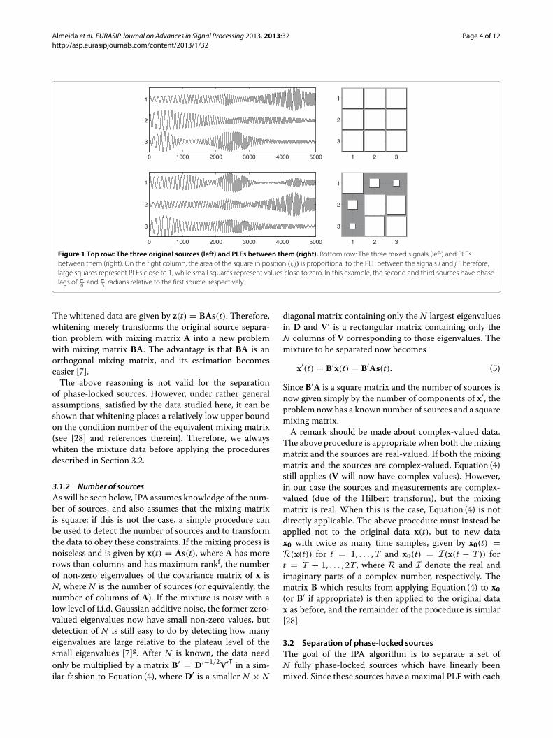
The effect of linear mixing on the PLF matrix is illus-trated in Figure 1 for a set of simulated sources. This sethas three sources, with PLFs of 1 with each other. Thesesources are of the form (1) with negligible phase jitter, andthe phase lags αj are 0, π

6 , andπ3 radians, respectively. The

common oscillation is a time-dependent sinusoid. Theamplitudes are generated by adding a small constant base-line to a random number of “bursts” with Gaussian shape.Each “burst” has a random center and a random width,and each source amplitude has 1 to 5 such “bursts”.The first row of Figure 1 shows on the left the original

sources and on the right their PLFmatrix. The second rowdepicts the mixed signals x(t) on the left and their PLFson the right; the mixing matrix has random entries uni-formly distributed between −1 and 1. It is clear that themixed signals have lower pairwise PLFs than the sources,although signals 2 and 3 still exhibit a rather high mutualPLF. This example suggests that linear mixing of syn-chronous sources reduces their synchrony, a fact that willbe proved in Section 3.3, ahead; this fact will be usedto extract the sources from the mixtures by trying tomaximize the PLF of the estimated sources.

3 AlgorithmIn this section, we describe the IPA algorithm. As men-tioned in Section 1, this algorithm first performs subspaceseparation, and then performs separation within each sub-space. In this article, we only study the performance ofIPA in the case where all the sources are phase-locked; inthis situation, the inter-subspace separation can entirelybe skipped, since there is only one subspace of lockedsources. Therefore, we will not discuss here the part of IPArelating to subspace separation; the reader is referred to[14] for a discussion on that subject.

3.1 Preprocessing3.1.1 WhiteningAs happens in ICA and other source separation tech-niques, whitening is a useful preprocessing step for IPA.Whitening, or sphering, is a procedure that linearlytransforms the data so that the transformed data havethe identity as its covariance matrix; in particular, thewhitened data are uncorrelated [7]. In ICA, there areclear reasons to pursue uncorrelatedness: independentdata are also uncorrelated, and therefore whitening thedata already fulfills one of the required conditions to findindependent sources. If D denotes the diagonal matrixcontaining the eigenvalues of the covariance matrix ofthe data and V denotes an orthonormal matrix whichhas, in its columns, the corresponding eigenvectors, thenwhitening can be performed in a PCA-like manner bymultiplying the data x(t) by a matrix B, where [7]

B = D−1/2VT. (4)

Almeida et al. EURASIP Journal on Advances in Signal Processing 2013, 2013:32 Page 4 of 12http://asp.eurasipjournals.com/content/2013/1/32

1 2 3

1

2

3

0 1000 2000 3000 4000 5000

3

2

1

1 2 3

1

2

3

0 1000 2000 3000 4000 5000

3

2

1

Figure 1 Top row: The three original sources (left) and PLFs between them (right). Bottom row: The three mixed signals (left) and PLFsbetween them (right). On the right column, the area of the square in position (i, j) is proportional to the PLF between the signals i and j. Therefore,large squares represent PLFs close to 1, while small squares represent values close to zero. In this example, the second and third sources have phaselags of π

6 and π3 radians relative to the first source, respectively.

The whitened data are given by z(t) = BAs(t). Therefore,whitening merely transforms the original source separa-tion problem with mixing matrix A into a new problemwith mixing matrix BA. The advantage is that BA is anorthogonal mixing matrix, and its estimation becomeseasier [7].The above reasoning is not valid for the separation

of phase-locked sources. However, under rather generalassumptions, satisfied by the data studied here, it can beshown that whitening places a relatively low upper boundon the condition number of the equivalent mixing matrix(see [28] and references therein). Therefore, we alwayswhiten the mixture data before applying the proceduresdescribed in Section 3.2.

3.1.2 Number of sourcesAswill be seen below, IPA assumes knowledge of the num-ber of sources, and also assumes that the mixing matrixis square: if this is not the case, a simple procedure canbe used to detect the number of sources and to transformthe data to obey these constraints. If the mixing process isnoiseless and is given by x(t) = As(t), where A has morerows than columns and has maximum rankf, the numberof non-zero eigenvalues of the covariance matrix of x isN, where N is the number of sources (or equivalently, thenumber of columns of A). If the mixture is noisy with alow level of i.i.d. Gaussian additive noise, the former zero-valued eigenvalues now have small non-zero values, butdetection of N is still easy to do by detecting how manyeigenvalues are large relative to the plateau level of thesmall eigenvalues [7]g. After N is known, the data needonly be multiplied by a matrix B′ = D′−1/2V′T in a sim-ilar fashion to Equation (4), where D′ is a smaller N × N

diagonal matrix containing only the N largest eigenvaluesin D and V′ is a rectangular matrix containing only theN columns of V corresponding to those eigenvalues. Themixture to be separated now becomes

x′(t) = B′x(t) = B′As(t). (5)

Since B′A is a square matrix and the number of sources isnow given simply by the number of components of x′, theproblem now has a known number of sources and a squaremixing matrix.A remark should be made about complex-valued data.

The above procedure is appropriate when both the mixingmatrix and the sources are real-valued. If both the mixingmatrix and the sources are complex-valued, Equation (4)still applies (V will now have complex values). However,in our case the sources and measurements are complex-valued (due of the Hilbert transform), but the mixingmatrix is real. When this is the case, Equation (4) is notdirectly applicable. The above procedure must instead beapplied not to the original data x(t), but to new datax0 with twice as many time samples, given by x0(t) =R(x(t)) for t = 1, . . . ,T and x0(t) = I(x(t − T)) fort = T + 1, . . . , 2T , where R and I denote the real andimaginary parts of a complex number, respectively. Thematrix B which results from applying Equation (4) to x0(or B′ if appropriate) is then applied to the original datax as before, and the remainder of the procedure is similar[28].

3.2 Separation of phase-locked sourcesThe goal of the IPA algorithm is to separate a set ofN fully phase-locked sources which have linearly beenmixed. Since these sources have a maximal PLF with each

Almeida et al. EURASIP Journal on Advances in Signal Processing 2013, 2013:32 Page 5 of 12http://asp.eurasipjournals.com/content/2013/1/32

other and the mixture components do not (as motivatedin Section 2.4 above and proved in Section 3.3 below), wecan unmix them by searching for projections that maxi-mize the resulting PLFs. Specifically, this corresponds tofinding aN×N matrixW such that the estimated sources,y(t) = WTx(t) = WTAs(t), have the highest possiblePLFs.The optimization problem that we shall solve is

maxW

(1 − λ)

N∑j,k=1j>k

2jk + λ log | detW| (6)

s.t. ‖wj‖ = 1, for j = 1, . . . ,N

where wj is the jth column ofW. In the first term, we sumthe squared PLFs between all pairs of sources. The secondterm penalizes unmixing matrices that are close to singu-lar, and λ is a parameter controlling the relative weightsof the two terms. This second term serves the purposeof preventing the algorithm from finding, e.g., solutionswhere two columns j and k of W are colinear, which triv-ially yields jk = 1 (a similar term is used in some ICAalgorithms [7]). Each column of W is constrained to haveunit norm to prevent trivial decreases of that term.The optimization problem in Equation (6) is highly non-

convex: the objective function is a sum of two terms, eachof which is non-convex in the variable W. Furthermore,the unit norm constraint is also non-convex. Despite this,as we show below in Section 3.3, it is possible to character-ize all the global maxima of this problem for the case λ = 0and to devise an optimization strategy taking advantage ofthat result.The above optimization problem can be tackled through

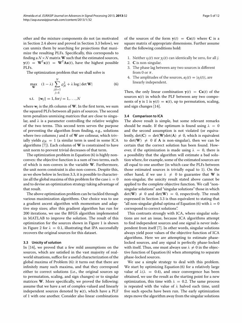
various maximization algorithms. Our choice was to usea gradient ascent algorithm with momentum and adap-tive step sizes; after this gradient algorithm has run for200 iterations, we use the BFGS algorithm implementedin MATLAB to improve the solution. The result of thisoptimization for the sources shown in Figure 1 is shownin Figure 2 for λ = 0.1, illustrating that IPA successfullyrecovers the original sources for this dataset.

3.3 Unicity of solutionIn [14], we proved that a few mild assumptions on thesources, which are satisfied in the vast majority of real-world situations, suffice for a useful characterization of theglobal maxima of Problem (6): it turns out that there areinfinitely many such maxima, and that they correspondeither to correct solutions (i.e., the original sources upto permutation, scaling, and sign changes) or to singularmatrices W. More specifically, we proved the following:assume that we have a set of complex-valued and linearlyindependent sources denoted by s(t), which have a PLFof 1 with one another. Consider also linear combinations

of the sources of the form y(t) = Cs(t) where C is asquare matrix of appropriate dimensions. Further assumethat the following conditions hold:

1. Neither sj(t) nor yj(t) can identically be zero, for all j.2. C is non-singular.3. The phase lag between any two sources is different

from 0 or π .4. The amplitudes of the sources, aj(t) = |sj(t)|, are

linearly independent.

Then, the only linear combination y(t) = Cs(t) of thesources s(t) in which the PLF between any two compo-nents of y is 1 is y(t) = s(t), up to permutation, scaling,and sign changes [14].

3.4 Comparison to ICAThe above result is simple, but some relevant remarksshould be made. If the optimum is found using λ = 0and the second assumption is not violated (or equiva-lently, det(C) = det(W)det(A) �= 0, which is equivalentto det(W) �= 0 if A is non-singular), then we can becertain that the correct solution has been found. How-ever, if the optimization is made using λ = 0, there isa possibility that the algorithm will estimate a bad solu-tion where, for example, some of the estimated sources areall equal to one another (in which case the PLFs betweenthose estimated sources is trivially equal to 1). On theother hand, if we use λ �= 0 to guarantee that W isnon-singular, the unicity result stated above cannot beapplied to the complete objective function. We call “non-singular solutions” and “singular solutions” those in whichdet(W) �= 0 and det(W) = 0, respectively. The resultexpressed in Section 3.3 is thus equivalent to stating that“all non-singular global optima of Equation (6) with λ = 0correspond to correct solutions”.This contrasts strongly with ICA, where singular solu-

tions are not an issue, because ICA algorithms attemptto find independent sources and one signal is never inde-pendent from itself [7]. In other words, singular solutionsalways yield poor values of the objective function of ICAalgorithms. Here we are attempting to estimate phase-locked sources, and any signal is perfectly phase-lockedwith itself. Thus, one must always use λ �= 0 in the objec-tive function of Equation (6) when attempting to separatephase-locked sources.We use a simple strategy to deal with this problem.

We start by optimizing Equation (6) for a relatively largevalue of λ(λ = 0.4), and once convergence has beenobtained, we use the result as the starting point for a newoptimization, this time with λ = 0.2. The same processis repeated with the value of λ halved each time, untilfive such epochs have been run. The early optimizationsteps move the algorithm away from the singular solutions

Almeida et al. EURASIP Journal on Advances in Signal Processing 2013, 2013:32 Page 6 of 12http://asp.eurasipjournals.com/content/2013/1/32

1 2 3

1

2

3

1 2 3

1

2

3

0 1000 2000 3000 4000 5000

3

2

1

Figure 2 The three sources estimated by IPA (left), PLFs between them (middle), and the gain matrixWTA (right). Black squares representnegative values of the gain matrix, while white squares represent positive values. Since the gain matrix is very close to a permutated diagonal matrix,we can conclude that IPA successfully recovered the sources, up to permutation, scaling, and sign change.

discussed above, whereas the final steps are done with avery low value of λ, where the above unicity conditions areapproximately valid. As the following experimental resultsshow, this strategy can successfully prevent singular solu-tions from being found, while making the influence of thesecond term of Equation (6) on the final result negligible.

4 Experimental results4.1 Data generationAs mentioned earlier, the main goal of this study is tostudy the applicability of IPA to real-world electrophysio-logical data from human brain EEG andMEG. The choiceof the data for this study was not trivial, since we needto know the true sources in order to quantitatively mea-sure the quality of the results. On the one hand, to knowthe actual sources in the brain would require simultane-ous data from outside the scalp (EEG or MEG, whichwould be the mixed signals) and from inside the scalp(intra-craneal recordings, corresponding to the sources).If intra-craneal recordings are not available, results can-not quantitatively be assessed; they can only qualitativelybe assessed by experts who can tell whether the extractedsources are meaningful or not. On the other hand, dueto their extreme simplicity, synthetic data such as thoseused so far to illustrate IPA, shown in Figure 1, cannot beused to assess the usefulness of the method in real-worldsituations.In an attempt to obtain “the best of both worlds”, we

have generated a pseudo-real dataset from actual MEGrecordings. By doing this, we know the true sources andthe true mixing matrix, while still using sources that are ofa nature similar to what one observes in real-world MEG.We begin by describing the process that we used to gen-erate a perfectly phase-locked dataset; we then explainhow we modified these data to analyze non-perfect casesas well. It is important to stress that the generation pro-cess described below has no relation to the one used togenerate the data of Figure 1, even though both processesgenerate sources with maximum PLF.

Our first step was to obtain a realistic mixing matrix.To do so, we used the well-known EEGIFT software pack-age [29]. This package includes a real-world sample EEGdataset with 64 channels. Using all the default options ofthe software package, we extracted 20 independent com-ponents from the data of Subject 1 in that dataset. Theresults that was important for us, in this process, werenot the independent components themselves (which werediscarded), but rather the 64 × 20 mixing matrix. As dis-cussed in Section 3.1, we have opted for using a squaremixing matrix, with little loss of generality. Therefore, weselected N random rows and N random columns of thatmixing matrix (without repetition), and formed an N ×Nmixing matrix from the corresponding values of the origi-nal 64 × 20 matrix. We will later show results for datasetsranging from N = 2 to N = 5 sources; in the following,assume, for the sake of concreteness, that N = 4.Having generated a physiologically plausible mixing

matrix, the next step was to generate a set of four sources.For this, we used the MEG dataset studied previously in[30]h, which has 122 channels with 17,730 samples perchannel. The sampling frequency is 297Hz, and the datahave already been subjected to low-pass filtering with cut-off at 90Hz. Since band-pass filtering is a very commonpreprocessing step in the analysis of MEG data [20-22]and is useful for the use of the Hilbert transform, weperformed a further band-pass filtering with no phasedistortion, keeping only the 18–24Hz bandi. The result-ing filtered data were used to generate a complex signalthrough the Hilbert transform; these data were whitenedas described in Section 3.1, and from the whitened datawe extracted the time-dependent amplitudes and phases.We then selected four random channels of these filtered

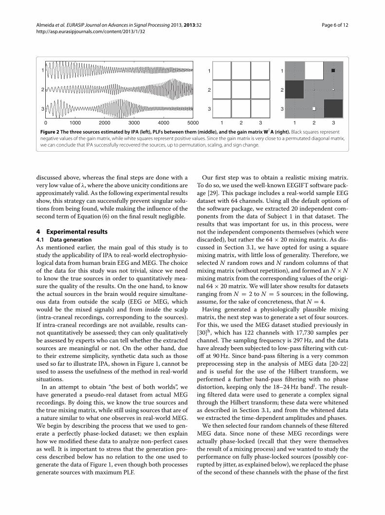
MEG data. Since none of these MEG recordings wereactually phase-locked (recall that they were themselvesthe result of a mixing process) and we wanted to study theperformance on fully phase-locked sources (possibly cor-rupted by jitter, as explained below), we replaced the phaseof the second of these channels with the phase of the first

Almeida et al. EURASIP Journal on Advances in Signal Processing 2013, 2013:32 Page 7 of 12http://asp.eurasipjournals.com/content/2013/1/32

channel with a constant phase lag of π6 radians. The phase

of the third channel was replaced with the phase of thefirst channel with a constant phase lag of π

3 radians, andthat of the fourth channel with the phase of the first chan-nel with a lag of π

2 radians. The amplitudes of the foursources were kept as the original amplitudes of the fourrandom channels themselves. The process is illustrated inFigure 3. The above process, including the choice of the4×4 submatrix, was repeated 100 times, with different ini-tializations of the random number generator. This way ofconstructing the data ensured that the sources were fullyphase-locked.We also constructed datasets in which the sources were

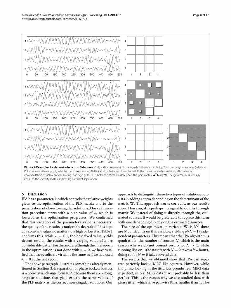
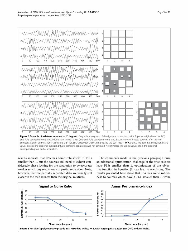
not perfectly phase locked. For this, we used the same 100sets of sources, but with those sources now corrupted byphase jitter: each sample t of each source j was multipliedby eiδj(t), where the phase jitter δj(t)was drawn from a ran-dom Gaussian distribution with zero mean and standarddeviation σ . We tested IPA for σ from 0 to 20 degrees, in5 degrees steps. One example with σ = 5 degrees is shownin Figure 4, and one with σ = 20 degrees is shown inFigure 5.Finally, we studied the effect of N on the results of

the proposed algorithm. We created 100 datasets simi-lar to the jitterless datasets mentioned earlier, using N =2, 3 and 5. In all of these, and similarly to the data withN = 4, we used sources with phase lags multiple of π

6 .

4.2 ResultsWe measured the separation quality using two measures:the Amari performance index (API) [31] and the well-known signal-to-noise ratio (SNR). The API measureshow far the gain matrix WTA is from a permutated diag-onal matrix; the SNR measures how far the estimatedsources are from the true sources. In summary, the APImeasures the quality of the estimation of the mixingmatrix, while the SNR measures the quality of the estima-tion of the sources themselves.Figure 6 presents the means and standard deviations of

these measures for the 100 runs mentioned in Section 4.1,for each of the jitter levels. The results indicate that IPA

has very good performance on the jitterless case, in dataof this kind, and that this level of performance is approx-imately maintained even in the presence of low levels ofphase jitter, up to 5 degrees of standard deviation. Somedeterioration in performance occurs from 5 to 10 degreesof phase jitter standard deviation, but with a SNR of 27 dBand an API below 0.1 the sources can still be consideredto be well estimated.The results for high jitter levels (sigma equal to 15 or

20 degrees) show that there is a limit to IPA’s robust-ness; this limit lies somewhere between 10 and 15 degrees.Equivalently, in terms of the PLF, the algorithm showsgood robustness to PLF values smaller than 1 as long asthey are above 0.95, but below that value its performancedeteriorates progressively up to a PLF of approximately0.9, at which point only partial separations are obtained.Figure 7 shows the effect of varying the number of

sources N. The figure shows that IPA can handle val-ues of N up to N = 5 with only a slight decrease inperformance.Figure 7 also shows something rather peculiar: for N =

2, the results are mediocre (with an average API around0.4)j. This is not an effect of lowering the number ofsources N, but rather an indirect effect of the phase lagbetween the sources. To verify this, we generated datasetsof jitterless data with N = 2, using phase lags of π

12 ,2π12

(the value used in Figure 7), 3π12 , and

4π12 (100 datasets for

each of these values). Figure 8 shows that a phase lag of 2π12

yields poor API values, as we already knew, but 3π12 yields

very good values. Naively, one could conclude that whenthe sources have a phase lag of 2π

12 , or less, the separationcannot be accurately performed.The effect is, however, not so clear-cut. The results for

N = 3, 4, 5 also involve sources with phase lags of π6 , but

the API values for those experiments are very good. Wedo not have a solid explanation for this fact; we conjec-ture that the presence of some pairs of sources with largerphase lags (e.g., for N = 4, the first and third sourceshave a phase lag of π

3 and the first and fourth sourceshave a phase lag of π

2 ) aids in the separation of all thesources.

Figure 3 The process used to generate the pseudo-real MEG sources.

Almeida et al. EURASIP Journal on Advances in Signal Processing 2013, 2013:32 Page 8 of 12http://asp.eurasipjournals.com/content/2013/1/32

1 2 3 4

1

2

3

4

0 50 100 150 200 250 300 350 400 450 500

4

3

2

1

1 2 3 4

1

2

3

4

0 50 100 150 200 250 300 350 400 450 500

4

3

2

1

1 2 3 4

1

2

3

4

1 2 3 4

1

2

3

4

0 50 100 150 200 250 300 350 400 450 500

4

3

2

1

Figure 4 Example of a dataset where σ = 5degrees. Only a short segment of the signals is shown, for clarity. Top row: original sources (left) andPLFs between them (right). Middle row: mixed signals (left) and PLFs between them (right). Bottom row: estimated sources, after manualcompensation of permutation, scaling, and sign (left); PLFs between them (middle); and the gain matrixWTA (right). The gain matrix is virtuallyequal to the identity matrix, indicating a correct separation.

5 DiscussionIPA has a parameter, λ, which controls the relative weightsgiven to the optimization of the PLF matrix and to thepenalization of close-to-singular solutions. Our optimiza-tion procedure starts with a high value of λ, which islowered as the optimization progresses. We confirmedthat this variation of the parameter’s value is necessary:the quality of the results is noticeably degraded if λ is keptat a constant value, nomatter how high or low it is. Table 1confirms this: while λ = 0.1, the best fixed value, yieldsdecent results, the results with a varying value of λ areconsiderably better. Furthermore, although the final epochin the optimization is not done with λ = 0, we have veri-fied that the results are virtually the same as if we had usedλ = 0 at the last epoch.The above paragraph illustrates something alreadymen-

tioned in Section 3.4: separation of phase-locked sourcesis a non-trivial change from ICA because there are wrong,singular solutions that yield exactly the same values ofthe PLF matrix as the correct non-singular solutions. Our

approach to distinguish these two types of solutions con-sists in adding a term depending on the determinant of thematrix W. This approach works correctly, as our resultsshow. However, it is perhaps inelegant to do this throughmatrix W, instead of doing it directly through the esti-mated sources. It would be preferable to replace this termwith one depending directly on the estimated sources.The size of the optimization variable, W, is N2; there

areN constraints on this variable, yieldingN(N −1) inde-pendent parameters. This means that the IPA algorithm isquadratic in the number of sources N, which is the mainreason why we do not present results for N > 5; whilerunning IPA on 100 datasets withN = 2 takes a few hours,doing so for N = 5 takes several days.The results that we obtained show that IPA can sepa-

rate perfectly locked MEG-like sources. However, whilethe phase locking in the jitterless pseudo-real MEG datais perfect, in real MEG data it will probably be less thanperfect. This is the reason why we also studied data withphase jitter, which have pairwise PLFs smaller than 1. The

Almeida et al. EURASIP Journal on Advances in Signal Processing 2013, 2013:32 Page 9 of 12http://asp.eurasipjournals.com/content/2013/1/32

1 2 3 4

1

2

3

4

0 50 100 150 200 250 300 350 400 450 500

4

3

2

1

1 2 3 4

1

2

3

4

0 50 100 150 200 250 300 350 400 450 500

4

3

2

1

1 2 3 4

1

2

3

4

1 2 3 4

1

2

3

4

0 50 100 150 200 250 300 350 400 450 500

4

3

2

1

Figure 5 Example of a dataset where σ = 20degrees. Only a short segment of the signals is shown, for clarity. Top row: original sources (left)and PLFs between them (right). Middle row: mixed signals (left) and PLFs between them (right). Bottom row: estimated sources, after manualcompensation of permutation, scaling, and sign (left); PLFs between them (middle); and the gain matrixWTA (right). The gain matrix has significantvalues outside the diagonal, indicating that a complete separation was not achieved. Nevertheless, the largest values are in the diagonal,corresponding to a partial separation.

results indicate that IPA has some robustness to PLFssmaller than 1, but the sources still need to exhibit con-siderable phase locking for the separation to be accurate;weaker synchrony results only in partial separation. Note,however, that the partially separated data are usually stillcloser to the true sources than the original mixtures.

The comments made in the previous paragraph raisean additional optimization challenge: if the true sourceshave PLFs smaller than 1, optimization of the objec-tive function in Equation (6) can lead to overfitting. Theresults presented here show that IPA has some robust-ness to sources which have a PLF smaller than 1, while

Figure 6 Result of applying IPA to pseudo-real MEG data withN = 4, with varying phase jitter: SNR (left) and API (right).

Almeida et al. EURASIP Journal on Advances in Signal Processing 2013, 2013:32 Page 10 of 12http://asp.eurasipjournals.com/content/2013/1/32

Figure 7 Effect of applying IPA to pseudo-real MEG data with varying values of N: SNR (left) and API (right).

being stationary (since the phase jitter is stationary, thedistribution of the PLF does not vary with time). In real-world cases, it is likely that the PLF is non-stationary:for example, some sources may be phase-locked at thestart of the observation period and not phase-lockedat its end. While simple techniques such as windowingcan be devised to tackle smaller time intervals wherestationarity is (almost) verified, one would still need tofind a way to integrate the information from differentintervals. Such integration is out of the scope of thisarticle.One interesting extension of this article would be the

separation of specific types of systems, such as van der Poloscillators [27]. For those, fully entrained oscillators mayeven present a PLF < 1, and a different measure of syn-chrony, tailored to those oscillators, may need to be used.Such a study would fall out of the scope of this article.Nevertheless, it is expected that additional knowledge ofthe oscillator type can be exploited to improve the algo-rithm’s performance or its robustness to deviations fromthe ideal case.One can derive a relationship between additive

Gaussian noise (e.g., from the sensors) and the phase jit-ter used throughout this article. Figure 5 depicts, in thecomplex plane, a sample of a noiseless signal x(t) ≡

a(t)eiφ(t), to which complex noise n(t) is added to formthe noisy signal xn ≡ a(t)eiφ(t) + n(t)k. That figurealso shows n⊥(t), which is the projection of n(t) onthe direction orthogonal to x(t), and xn⊥(t) ≡ x(t) +n⊥(t). Also depicted are φ(t), φn(t) and φn⊥(t), whichare defined as the phases of x(t), xn(t) and xn⊥(t),respectively.It can easily be shown that, if |n(t)| << |x(t)| = a(t),

then φn(t) ≈ φn⊥(t) ≈ φ(t) + n⊥(t)a(t) [32]. This is an

important relationship, because it shows that, under addi-tive noise, portions of the signal with a large amplitudewill have a better phase estimate than portions with asmall amplitude, in which even small amounts of additivenoise can severely disrupt the phase estimation. We thusbelieve that the PLF quantity, while attractive and elegantin theory, and despite working well with low amounts ofadditive noise [14], will probably need to be changed tofactor in the amplitude in an appropriate way to deal withapplications where considerable amounts of additive noiseare present.

6 ConclusionWe have shown that IPA can successfully separate phase-locked sources from linear mixtures in pseudo-real MEGdata. We showed that IPA tolerates deviations from the

Figure 8 Effect of applying IPA to pseudo-real MEG data with varying phase lags between the sources, withN = 2: SNR (left) and API(right).

Almeida et al. EURASIP Journal on Advances in Signal Processing 2013, 2013:32 Page 11 of 12http://asp.eurasipjournals.com/content/2013/1/32

Table 1 Values of SNR and API for jitterless data with N = 3, for various fixed values of λ, as well as for thevarying-lambda strategy detailed in the text

λ 0.025 0.05 0.1 0.2 0.4

SNR Fixed 17.5 ± 21.2 27.5 ± 18.0 34.4 ± 4.3 27.2 ± 3.6 13.5 ± 5.5

Varying 48.9 ± 8.7

API Fixed 0.795 ± 0.570 0.369 ± 0465 0.048 ± 0.057 0.079 ± 0.027 0.327 ± 0.097

Varying 0.013 ± 0.015

While the best fixed value, λ = 0.1, yields decent results, the results using a varying value of λ are consistently better, with a large margin.

ideal case, yielding excellent results for low amounts ofphase jitter, and that it exhibits some robustness to mod-erate amounts of phase jitter. We also showed that it canhandle numbers of sources up to N = 5. We believethat these results bring us closer to the goal of suc-cessfully separating phase-locked sources in real-worldsignals.

EndnotesaIn EEG and MEG, the sources are not individual neu-rons, whose oscillations are too weak to be detectedfrom outside the scalp. In these cases, the sourcesare populations of closely located neurons oscillatingtogether.bThe term “real-valued” is used here to distinguish fromother phase-based algorithms where a complex quantityis used [14].cTechnically, this condition could be violated in a set withzero measure. Since we will deal with a discrete and finitenumber of time points, no such sets exist and this techni-cality is not important.dWe will also show results where this phase difference isnot exactly constant; see Figure 6.

Figure 9 Diagram illustrating the relationship between phasejitter and additive noise. A single time sample is shown, and thetime argument has been dropped for simplicity.

eThese assumptions are not as restrictive as they maysound; see Section 3.1.fThis is usually called the over-determined case. Theunder-determined case, where A has fewer rows thancolumns, is more difficult and is not addressed here.gThere are more rigorous criteria that can be used tochoose N. Two very popular methods are the Akaikeinformation criterion and the minimum descriptionlength. It is out of the scope of this article to discuss thesetwo criteria; the reader is referred to [7] and referencestherein for more information.hFreely available from http://research.ics.tkk.fi/ica/eegmeg/MEG data.html.iThe choice of this specific band is rather arbitrary. Theband is narrow enough that the Hilbert transform willallow correct estimation of instantaneous amplitude andphase, but wide enough that the instantaneous frequencyof the signals retains some variability. The passband is alsoof a similar width as in typical studies using MEG [20].jIt might appear contradictory that the average SNR has agood value, 40 dB, when the average API has a mediocrescore. In reality, when the standard deviation of the SNRis very high, it is usually an indication that the separationis poor. As an example, consider a case where one sourceis very well estimated, with an SNR of 80 dB, and one ispoorly estimated, with an SNR of 0 dB. The average SNRwould be 40, but with a very high standard-deviation.Good values of the average SNR are indicators of a goodseparation only when the standard-deviation of the SNRis small.kIn most real applications, one will be dealing with mod-els consisting of real signals to which real-valued noiseis added. However, the linearity of the Hilbert transformallows the same type of analysis for that case as for thecase of complex signals with complex additive noisewhich is considered here.

Competing interestsThe author declare that they have no competing interests.

AcknowledgementsThis work was partially supported by project DECA-Bio of Instituto deTelecomunicacoes, PEst-OE/EEI/LA0008/2011.

Author details1Instituto de Telecomunicacoes, Lisbon, Portugal. 2Aalto University School ofScience, Espoo, Finland.

Almeida et al. EURASIP Journal on Advances in Signal Processing 2013, 2013:32 Page 12 of 12http://asp.eurasipjournals.com/content/2013/1/32

Received: 1 April 2012 Accepted: 2 February 2013Published: 22 February 2013

References1. M A Pikovsky, J Rosenblum, Kurths, Synchronization: A Universal Concept in

Nonlinear Sciences. (Cambridge Nonlinear Science Series (CambridgeUniversity Press), Cambridge, MA, 2001)

2. JM Palva, S Palva, K Kaila, Phase synchrony among neuronal oscillations inthe human cortex. J. Neurosci. 25(15), 3962–3972 (2005)

3. JM Schoffelen, R Oostenveld, P Fries, Imaging the human motor system’sbeta-band synchronization during isometric contraction. NeuroImage.41, 437–447 (2008)

4. PJ Uhlhaas, W Singer, Neural synchrony in brain disorders: relevance forcognitive dysfunctions and pathophysiology. Neuron. 52, 155–168 (2006)

5. PL Nunez, R Srinivasan, AF Westdorp, RS Wijesinghe, DM Tucker, RBSilberstein, PJ Cadusch, EEG coherency I: statistics, reference electrode,volume conduction, Laplacians, cortical imaging, and interpretation atmultiple scales. Electroencephalogr. Clin. Neurophysiol.103, 499–515 (1997)

6. R Vigario, J Sarela, V Jousmaki, M Hamalainen, E Oja, Independentcomponent approach to the analysis of EEG and MEG recordings. IEEETrans. Biomed. Eng. 47(5), 589–593 (2000)

7. A Hyvarinen, J Karhunen, E Oja, Independent Component Analysis.(Wiley, New York, 2001)

8. M Akhtar, W Mitsuhashi, C James, Employing spatially constrained ICAand wavelet denoising for automatic removal of artifacts frommultichannel EEG data. Signal Process. 92, 401–416 (2012)

9. M de Vos, L de Lathauwer, S van Huffel, Spatially constrained ICAalgorithm with an application in EEG processing. Signal Process.91, 1963–1972 (2011)

10. D Lee, H Seung, Algorithms for non-negative matrix factorization. Adv.Neural Inf. Process. Syst. 13, 556–562 (2001)

11. TH Chan, WK Ma, CY Chi, Y Wang, A convex analysis framework for blindseparation of non-negative sources. IEEE Trans. Signal Process.56, 5120–5134 (2008)

12. R de Frein, S Rickard, The synchronized short-time-Fourier-transform:properties and definitions for multichannel source separation. IEEE Trans.Signal Process. 59, 91–103 (2011)

13. S Hosseini, Y Deville, H Saylani, Blind separation of linear instantaneousmixtures of non-stationary signals in the frequency domain. SignalProcess. 89, 819–830 (2009)

14. M Almeida, JH Schleimer, J Bioucas-Dias, R Vigario, Source separation andclustering of phase-locked subspaces. IEEE Trans. Neural Netw.22(9), 1419–1434 (2011)

15. M Almeida, J Bioucas-Dias, R Vigario, in Proceedings of the InternationalConference on Independent Component Analysis and Signal Separation,vol. 6365. Independent phase analysis: separating phase-lockedsubspaces, (2010), pp. 189–196

16. A Ziehe, KR Muller, in International Conference on Artificial Neural Networks.TDSEP—an efficient algorithm for blind separation using time structure,(1998), pp. 675–680

17. C Torrence, GP Compo, A practical guide to wavelet analysis. Bull. Am.Meteorol. Soc. 79, 61–78 (1998)

18. AV Oppenheim, RW Schafer, JR Buck, Discrete-Time Signal Processing.(Prentice-Hall International Editions, Englewood Cliffs, NJ, 1999)

19. MLV Quyen, J Foucher, JP Lachaux, E Rodriguez, A Lutz, J Martinerie,FJ Varela, Comparison of Hilbert transform and wavelet methods for theanalysis of neuronal synchrony. J. Neurosci. Methods. 111, 83–98 (2001)

20. F Varela, JP Lachaux, E Rodriguez, J Martinerie, The Brainweb: phasesynchronization and large-scale integration. Nat. Rev. Neurosci.2, 229–239 (2001)

21. E Niedermeyer, FHL da Silva, Electroencephalography: Basic Principles,Clinical Applications, and Related Fields. (Lippincott Williams and Wilkins,Philadelphia, 2005)

22. P Nunez, R Srinivasan, Electric Fields of the Brain: the Neurophysics of EEG.(Oxford University Press, New York, 2006)

23. B Gold, AV Oppenheim, CM Rader, in Symposium on Computer Processingin Communications. Theory and implementation of the discrete Hilberttransform, (1973)

24. M Breakspear, S Heitmann, A Daffertshofer, Generative models of corticaloscillations: neurobiological implications of the Kuramoto model. Front.Human Neurosci. 4, 190–202 (2010)

25. Y Kuramoto, Chemical Oscillations, Waves and Turbulences.(Springer, Berlin, 1984)

26. S Strogatz, Nonlinear Dynamics and Chaos. (Westview Press, Boulder, 2000)27. E Izhikevich, Dynamic Systems in Neuroscience. (MIT Press, Cambridge,

MA, 2007)28. M Almeida, R Vigario, J Bioucas-Dias, in Proceedings of the International

Conference on Latent Variable Analysis and Signal Separation, vol. 7191. Therole of whitening for separation of synchronous sources, (2012),pp. 139–146

29. T Eichele, S Rachakonda, B Brakedal, R Eikeland, VD Calhoun, EEGIFT:group independent component analysis for event-related EEG data.Comput. Intell. Neurosci. 2011, 1–9 (2011)

30. R Vigario, V Jousmaki, M Hamalainen, R Hari, E Oja, in Advances in NIPS.Independent component analysis for identification of artifacts inmagnetoencephalographic recordings, (1997)

31. S Amari, A Cichocki, HH Yang, in Advances in NIPS, vol. 8. A new learningalgorithm for blind signal separation, (1996), pp. 757–763

32. A Carlson, P Crilly, J Rutledge. Communication Systems: An Introductionto Signals and Noise in Electrical Communication (McGraw-Hill,New York, 2001)

doi:10.1186/1687-6180-2013-32Cite this article as: Almeida et al.: Separation of phase-locked sources inpseudo-real MEG data. EURASIP Journal on Advances in Signal Processing 20132013:32.

Submit your manuscript to a journal and benefi t from:

7 Convenient online submission

7 Rigorous peer review

7 Immediate publication on acceptance

7 Open access: articles freely available online

7 High visibility within the fi eld

7 Retaining the copyright to your article

Submit your next manuscript at 7 springeropen.com