1

Alkaline & Polymer Experimental Study for the 8TH & 16TH Reservoirs of the Matzen

Field

Christophe Van Laer Chair of Reservoir Engineering

Montanuniversität Leoben

Master Thesis Leoben, 2016

2

Abstract

An experimental investigation was conducted to test the potential of alkaline and polymer flooding to improve the recovery of the 8TH and 16TH reservoirs of the Matzen field, two reservoirs that have been producing for over 60 years. The investigation involved running an emulsion and a core flooding study.

In the emulsion study, various alkaline solutions were mixed with stock tank oil from the 8TH reservoir. The goal of the study was to observe how alkaline salt and concentration, reservoir brine, solution salinity and aquous/crude volume ratio influence the formation of emulsions. The results showed that no micro-emulsion would form due to the high salinity of the reservoir. It was also found that Na2CO3

is tolerant to divalent ions, unlike NaOH, however without the addition of EDTA precipitation occurs.

In the core flooding study, aged cores were flooded with different alkaline solutions and the following properties were measured: oil rate, water rate, pH, tracer concentration and polymer concentration. The most effective flood tested resulted in an incremental recovery factor of 0.331. The flood was composed of alkaline (1%wt Na2CO3), polymer (800ppm FLOPAM 3630s) and softened synthetic brine to inhibit precipitation. The experiments also indicated that alkaline is the major contributor to the recovery and that the polymer is indeed improving the sweep efficiency.

3

Kurzfassung

Um die Ausbeutung des 8TH und 16TH Speichergestein ins Matzen Erdöllagerstätte zu verbessern wurde eine experimentelle Untersuchung angelegt die das fluten mit alkalische und polymer Lösungen testet. Beide Speicher haben für mehr als 60 Jahre produziert. Die Untersuchung beinhaltet sowohl eine Emulsion Studie als auch das fluten von Bohrkernen. In der Emulsion Studie wurden verschiedene alkalische Lösungen mit Öle vom 8TH Speicher gemischt . Die Zielsetzung der Studie war das Aufnehmen der Beobachtungen wie verschiedene Alkalische Salze, deren Konzentrationen, Speicher Gewässer, Salzhaltigkeit und das O/W Volumen Verhältnis die Emulsion Bildung beeinflussen. Es wurde auch festgestellt, das im Gegensatz zu NaOH, Na2CO3 tolerant ist zu zweiwertige Ionen, jedoch ohne EDTA treten Fällungen auf. In der Fluten Studie wurden ältere Bohrkerne eingepumpt mit verschiedenen alkalische Lösungen und folgende Eigenschaften gemessen: Öl und Wasser Fließrate, pH-Wert, Tracer-Konzentration und Polymer Konzentration. Das wirksamste Fluten erreichte eine inkrementelle ausbeute (recovery factor) von 0.331. Die Aufstellung der beste Lösung beinhaltet Alkali (1%wt Na2CO3), Polymer (800ppm FLOPAM 3630s) und synthetische Enthärtungsmittel für das hindern der Fällungen. Die Experimente zeigen das die alkalische Lösungen den größten Beitrag zur Ausbeute haben und dass das Polymer die Durchflussleistung verbessert.

4

5

Acknowledgements

I would like to thank Dr. Torsten Clemens and Dr. Thomas Gumpenberger for giving me the opportunity to work on this project and for their guidance throughout the project. I would like to thank everyone at the OMV laboratories in Gänserndorf for helping me in various ways. A special thanks goes to Leopold Huber and Dr. Christoph Puls for helping me technically in the laboratory. Without their help I would not have been able to complete this project. I would also like to thank Dr. Holger Ott for reviewing my thesis.

Lastly, I would like to thank my family for all the support they gave me throughout the years. Thank you for your love, care and patience. Here is your receipt!

6

Contents Chapter 1: Introduction ......................................................................................................................... 14

Chapter 2: Literature Review ................................................................................................................ 14

2.1 Alkaline Flooding ......................................................................................................................... 15

2.1.1 Alkaline Salts ......................................................................................................................... 15

2.1.2 Alkaline Reaction with Crude ............................................................................................... 17

2.1.3 Alkaline Reaction with Rock ................................................................................................. 18

2.1.4 Alkaline Reaction with Hard Water ...................................................................................... 19

2.1.5 Alkaline Recovery Mechanisms ............................................................................................ 19

2.2 Polymer Flooding ......................................................................................................................... 20

2.2.1 Polymer Types ...................................................................................................................... 20

2.2.2 Non-Newtonian Properties of Polymers .............................................................................. 21

2.2.3 Polymer behavior within Porous Media ............................................................................... 22

2.3 Alkaline and Polymer Flooding .................................................................................................... 22

2.3.1 Types of Alkaline and Polymer Floods .................................................................................. 22

2.3.2 Polymer Effect on the pH ..................................................................................................... 23

2.3.3 Alkaline Effect on Polymer Viscosity .................................................................................... 23

2.3.4 Polymer Effect on Alkaline/Oil IFT ........................................................................................ 24

2.3.5 Polymer Adsorption in Polymer Alkaline System ................................................................. 25

Chapter 3: Geologic Background ........................................................................................................... 25

3.1 The Matzen Field ......................................................................................................................... 25

3.2 Reservoir of Interest-16TH Background Information .................................................................. 26

3.3 Reservoir of Interest-8TH Background Information .................................................................... 28

Chapter 4: Emulsion Study .................................................................................................................... 29

4.1 Introduction ................................................................................................................................. 29

4.2 Experiments & Results ................................................................................................................. 30

4.2.1 Initial Experiments ................................................................................................................ 30

4.2.2 Alkaline Experiments Without the Influence of Brine .......................................................... 30

4.2.3 Salinity Experiments ............................................................................................................. 31

4.2.4 EDTA Experiments ................................................................................................................ 32

4.3 Concluding Remarks .................................................................................................................... 33

Chapter 5: Core Flood Study ................................................................................................................. 33

5.1 Introduction ................................................................................................................................. 33

5.2 Flood Design ................................................................................................................................ 34

7

5.2.1 Flood Compositions .............................................................................................................. 34

5.3 Experiment Preparation & Procedure ......................................................................................... 37

5.3.1 Conventional Core Analysis .................................................................................................. 38

5.3.2 Core Sleeving ........................................................................................................................ 39

5.3.3 Core Saturation Process ....................................................................................................... 40

5.3.4 Core Flooding Procedure ...................................................................................................... 41

5.3.5 Data Gathering Procedure .................................................................................................... 42

5.3 Core Flooding Results .................................................................................................................. 45

5.3.1 Recovery Curves ................................................................................................................... 47

5.3.2 Tracer Curves ........................................................................................................................ 51

5.3.3 pH Curves.............................................................................................................................. 52

5.3.3 Polymer Concentration Curves ............................................................................................. 53

5.3.4 Concluding Remarks ............................................................................................................. 54

Chapter 6: Conclusion ........................................................................................................................... 54

Chapter 7: References ........................................................................................................................... 56

APPENDIX A: Data of Important Properties .......................................................................................... 58

A.1 Figures ......................................................................................................................................... 58

A.2 Tables .......................................................................................................................................... 58

APPENDIX B: Emulsion Study Data ........................................................................................................ 61

B.1 Figures of Emulsion Study ........................................................................................................... 61

B1.1 Figures of Initial Experiments ................................................................................................ 61

B.1.2 Figures of Alkaline experiments without the influence of Brine (Na2CO3) .......................... 62

B.1.3 Figures of Alkaline experiments without the influence of Brine (NaOH) ............................. 64

B.1.4 Figures of Salinity Experiments (Na2CO3) ............................................................................. 67

B.1.5 Figures of Salinity Experiments (NaOH) ............................................................................... 70

B.1.6 Figures of EDTA Experiments (Na2CO3) ................................................................................ 73

B.1.7 Figures of EDTA Experiments (NaOH) .................................................................................. 74

B.2 Tables of Emulsion Study ............................................................................................................ 76

APPENDIX C: Important Calculations..................................................................................................... 80

C.1 Irreducible Water Saturation & Original Oil in Place .................................................................. 80

C.2 Recovery Curves .......................................................................................................................... 80

C.3 Polymer Curves............................................................................................................................ 81

8

List of Figures Figure 2.1 Graph of pH values of alkaline solutions at different concentration at 25°C. .................... 16 Figure 2.2 Dynamic IFT between a crude oil and NaOH solutions at different concentrations. .......... 17 Figure 2.3 Schematic of alkaline recovery process (deZabala 1982). ................................................... 17 Figure 2.4 Effect of acid number on dynamic IFT (30°C). ...................................................................... 18 Figure 2.5 Table showing alkalinity loss (meq/kg) by minerals (Ehrlich and Wygal 1977; Mohnot and Bae 1989). .............................................................................................................................................. 18 Figure 2.6 Effects of alkali precipitation of flow experiments with different hardness solutions. ....... 19 Figure 2.7 Structure of partially hydrolyzed polyacrylamide (Dominguez and Willhite 1977). ............ 21 Figure 2.8 Polymer solution viscosity with respect to shear rate and polymer concentration (Pope, Wang, and Tsaur 1979). ........................................................................................................................ 21 Figure 2.9 Polymer solution viscosity with respect to shear rate at various brine salinities (Martin et al. 1983). ................................................................................................................................................ 21 Figure 2.10 Comparison of residual oil recovery factors in alkaline flood, polymer flood and the various combinations of the two (Katsanis, Krumrine, and Falcone 1983). ......................................... 23 Figure 2.11 Graph plotting changes of pH with exposure time (Sheng 1994). ..................................... 23 Figure 2.12 NaOH-HPAM solution viscosity with respect to time. ....................................................... 24 Figure 2.13 Alkaline effect on polymer (1000 mg/L 1275A) viscosity (Kang 2001). ............................. 24 Figure 2.14 Effects of polymer hydrolysis, type of alkali and exposure time with crude on IFT. ......... 25 Figure 3.1 General location of the Matzen Field. (Gruenwalder, Poellitzer, and Clemens 2007) ........ 25 Figure 3.2 Stratigraphy of the Matzen reservoir in the Middle Miocene (Hölzel M. 2010). ................ 26 Figure 3.3 Transgression of the Matzen Sand (16th – Main Pool), onlapping on older sediments (Kienberger and Fuchs 2006)................................................................................................................. 27 Figure 3.4 Production of the 16TH ........................................................................................................ 28 Figure 3.5 Production of the 8TH .......................................................................................................... 29 Figure 3.6 Top structure map of the 8TH reservoir. ............................................................................. 29 Figure 5.1 Summary of flood compositions. ......................................................................................... 37 Figure 5.2 Outcrop Beare sandstone core samples used. ..................................................................... 38 Figure 5.3 Merucry bath experiment to measure core bulk volume. ................................................... 38 Figure 5.4 Porosimeter equipment used to measure pore volume. ..................................................... 38 Figure 5.5 Permeamter equipment used to measure absolute permeability. ..................................... 39 Figure 5.6 Glueing process of the cores. ............................................................................................... 39 Figure 5.7 Final result of glueeing process. ........................................................................................... 40 Figure 5.8 Cores being bathed in synthethic brine at low pressure. .................................................... 40 Figure 5.9 Stock tank oil of the 8TH reservoir being filtered and degassed. ........................................ 41 Figure 5.10 Experimental set-up for drainage flooding process. .......................................................... 41 Figure 5.11 Phase experiment for live oil.............................................................................................. 42 Figure 5.12 Core flood experiment set-up. ........................................................................................... 42 Figure 5.13 separator with a solenoid magnetic valve. ........................................................................ 43 Figure 5.14 New seperator designed by Leopold Huber....................................................................... 44 Figure 5.15 Base Scenario Recovery Curves. ......................................................................................... 48 Figure 5.16 Alkaline Scenario Recovery Curves. ................................................................................... 49 Figure 5.17 Polymer Scenario Recovery Curves. ................................................................................... 49 Figure 5.18 Alkaline & Polymer Scenario Recovery Curves. ................................................................. 50

9

Figure 5.19 Average incremental recovery factors with error bars. ..................................................... 51 Figure 5.20 Tracer concentration curves for floods containing polymer. ............................................. 52 Figure 5.21 Tracer concentration curves for floods containing only alkaline. ...................................... 52 Figure 5.22 pH concentration curves. ................................................................................................... 53 Figure 5.23 Polymer cummulative recovery curves. ............................................................................. 53 Figure A. 1 Viscosity and density as a function of temperature of stock tank oil coming from the 8TH reservoir. ............................................................................................................................................... 58 Figure B. 1 0.10 % wt Na2CO3 in reservoir Brine Solution at different oil-solution ratios. .................. 61 Figure B. 2 0.25 % wt Na2CO3 in reservoir Brine Solution at different oil-solution ratios. .................. 61 Figure B. 3 0.50 % wt Na2CO3 in reservoir Brine Solution at different oil-solution ratios. .................. 61 Figure B. 4 0.009 n/L OH- ion concentration by dissolving Na2CO3 into distilled Water at different oil-solution ratios. ....................................................................................................................................... 62 Figure B. 5 0.024 n/L OH- ion concentration by dissolving Na2CO3 into distilled Water at different oil-solution ratios. ....................................................................................................................................... 62 Figure B. 6 0.047 n/L OH- ion concentration by dissolving Na2CO3 into distilled Water at different oil-solution ratios. ....................................................................................................................................... 62 Figure B. 7 0.094 n/L OH- ion concentration by dissolving Na2CO3 into distilled Water at different oil-solution ratios. ....................................................................................................................................... 63 Figure B. 8 0.142 n/L OH- ion concentration by dissolving Na2CO3 into distilled Water at different oil-solution ratios. ....................................................................................................................................... 63 Figure B. 9 0.009 n/L OH- ion concentration by dissolving NaOH into distilled Water at different oil-solution ratios. ....................................................................................................................................... 64 Figure B. 10 0.024 n/L OH- ion concentration by dissolving NaOH into distilled Water at different oil-solution ratio. ........................................................................................................................................ 64 Figure B. 11 0.047 n/L OH- ion concentration by dissolving NaOH into distilled Water at different oil-solution ratios. ....................................................................................................................................... 64 Figure B. 12 0.094 n/L OH- ion concentration by dissolving NaOH into distilled Water at different oil-solution ratios. ....................................................................................................................................... 65 Figure B. 13 0.142 n/L OH- ion concentration by dissolving NaOH into distilled Water at different oil-solution ratios. ....................................................................................................................................... 65 Figure B. 14 0.165 n/L OH- ion concentration by dissolving NaOH into distilled Water at different oil-solution ratios. ....................................................................................................................................... 65 Figure B. 15 0.189 n/L OH- ion concentration by dissolving NaOH into distilled Water at different oil-solution ratios. ....................................................................................................................................... 66 Figure B. 16 0.236 n/L OH- ion concentration by dissolving NaOH into distilled Water at different oil-solution ratios. ....................................................................................................................................... 66 Figure B. 17 0.009 n/L Na2CO3 Concentration at various NaCl wt% concentrations mixed at oil-solution ratios of 7:3. ............................................................................................................................ 67 Figure B. 18 0.024 n/L Na2CO3 Concentration at various NaCl wt% concentrations mixed at oil-solution ratios of 7:3. ............................................................................................................................ 67 Figure B. 19 .047 n/L Na2CO3 Concentration at various NaCl wt% concentrations mixed at oil-solution ratios of 7:3. .......................................................................................................................................... 68

10

Figure B. 20 0.071 n/L Na2CO3 Concentration at various NaCl wt% concentrations mixed at oil-solution ratios of 7:3. ............................................................................................................................ 68 Figure B. 21 0.094 n/L Na2CO3 Concentration at various NaCl wt% concentrations mixed at oil-solution ratios of 7:3. ............................................................................................................................ 69 Figure B. 22 0.009 n/L NaOH Concentration at various NaCl wt% concentrations mixed at oil-solution ratios of 7:3. .......................................................................................................................................... 70 Figure B. 23 0.024 n/L NaOH Concentration at various NaCl wt% concentrations mixed at oil-solution ratios of 7:3. .......................................................................................................................................... 70 Figure B. 24 0.047 n/L NaOH Concentration at various NaCl wt% concentrations mixed at oil-solution ratios of 7:3. .......................................................................................................................................... 71 Figure B. 25 0.071 n/L NaOH Concentration at various NaCl wt% concentrations mixed at oil-solution ratios of 7:3. .......................................................................................................................................... 71 Figure B. 26 0.094 n/L NaOH Concentration at various NaCl wt% concentrations mixed at oil-solution ratios of 7:3. .......................................................................................................................................... 72 Figure B. 27 0.009 n/L Na2CO3 Concentration at various EDTA concentrations (multiples of the optimum concentration) mixed at oil-solution ratios of 7:3. ................................................................ 73 Figure B. 28 0.024 n/L Na2CO3 Concentration at various EDTA concentrations (multiples of the optimum concentration) mixed at oil-solution ratios of 7:3. ................................................................ 73 Figure B. 29 0.047 n/L Na2CO3 Concentration at various EDTA concentrations (multiples of the optimum concentration) mixed at oil-solution ratios of 7:3. ................................................................ 73 Figure B. 30 0.071 n/L Na2CO3 Concentration at various EDTA concentrations (multiples of the optimum concentration) mixed at oil-solution ratios of 7:3. ................................................................ 74 Figure B. 31 0.009 n/L NaOH Concentration at various EDTA concentrations (multiples of the optimum concentration) mixed at oil-solution ratios of 7:3. ................................................................ 74 Figure B. 32 0.024 n/L NaOH Concentration at various EDTA concentrations (multiples of the optimum concentration) mixed at oil-solution ratios of 7:3. ................................................................ 74 Figure B. 33 0.047 n/L NaOH Concentration at various EDTA concentrations (multiples of the optimum concentration) mixed at oil-solution ratios of 7:3. ................................................................ 75 Figure B. 34 0.071 n/L NaOH Concentration at various EDTA concentrations (multiples of the optimum concentration) mixed at oil-solution ratios of 7:3. ................................................................ 75

11

List of Tables Table 3.1 16TH reservoir characteristics. .............................................................................................. 27 Table 3.2 8TH reservoir characteristics. ................................................................................................ 28 Table 5.1 Constant flood properties. .................................................................................................... 34 Table 5.2 Base Scenario flood composition. ......................................................................................... 35 Table 5.3 Alkaline Scenario-case 1 flood composition. ......................................................................... 35 Table 5.4 Alkaline Scenario-case 2 flood composition. ......................................................................... 35 Table 5.5 Alkaline Scenario-case 3 flood composition. ......................................................................... 36 Table 5.6 Polymer Scenario flood composition. .................................................................................... 36 Table 5.7 Alkaline & Polymer Scenario -case 1 flood composition. ...................................................... 36 Table 5.8 Alkaline & Polymer Scenario -case 2 flood composition. ...................................................... 37 Table 5.9 EOR flood composition for each core. ................................................................................... 46 Table 5.10 Average total recovery data. ............................................................................................... 47 Table 5.11 Average incremental recovery data. ................................................................................... 51 Table 5.12 Polymer recovery data. ....................................................................................................... 54

Table A. 1 Synthetic brine composition, mimicking the 8th reservoir of the Matzen field. .................. 58 Table A. 2 CCA data for each core. ........................................................................................................ 59 Table A. 3 Experiment data required for Core Flood saturation calculations. ..................................... 59 Table A. 4 Core flooding experiment sum ............................................................................................ 60

Table B. 1 Concentration of OH- ions for each set and the weight required for each salt. .................. 76 Table B. 2 Salinities for each NaOH Salinity experiment. ..................................................................... 77 Table B. 3 Salinities for each Na2CO3 salinity experiment. .................................................................. 79 Table B. 4 EDTA concentrations used in EDTA experiments. ................................................................ 79

12

Notation

EOR, Enhanced oil recovery.

IFT, Interfacial tension.

TH, Torton Horizon.

HA, Highly oil soluble pseudo-acid component.

IPV, Inacessible pore volume.

AP, Alkaline & Polymer.

K, Permeability.

Ø, Porosity.

σ, Standard deviation.

R.F, Recovery factor.

13

Chapter 1: Introduction The average recovery factor for oil reservoirs that have undergone secondary recovery techniques ranges between 15-40% (Brouwer et al. 2001).To understand why this recovery value is so poor it is necessary to clarify what occurs in the reservoir as its being depleted. As the hydrocarbons are being produced there is an ongoing influx of water into the reservoir; coming either from an aquifer or an injection well in a water flooding scenario. As the water saturation increases the remaining oil becomes more disconnected and trapped within the water phase. Moore, Slobob and others demonstrated this behavior with the usage of the pore-doublet model (Moore and Slobod 1955).The now trapped oil (residual oil) is much harder to remobilize due to the “Jamming Effect” which is the development of a capillary pressure drop across the disconnected fluid phase (McDougall and Sorbie 1993). This effect can be seen as an additional resistance to flow, making discontinuous oil much harder to produce than continuous oil. The Matzen field, in Austria, has been producing for over 60 years and some of its most productive reservoirs have been water flooded for over 40 years. It is safe to assume that at these conditions much of its oil has become trapped and, in order to be displaced, requires the implementation of enhanced recovery mechanisms.

Several different enhanced oil recovery (EOR) methods have been designed to improve a reservoir’s recovery, once it has reached these residual conditions. Their functionality rely either on decreasing the properties that dominate the capillary forces or increasing the properties that dominate the viscous forces. The magnitude of the capillary forces is defined by the interfacial tension (IFT), the wettability and the pore geometry .While the magnitude of the viscous forces is defined by the velocity and viscosity of the injected fluid. Throughout this study two EOR methods are investigated; alkaline and polymer flooding. Alkaline flooding can generate in-situ surfactant, decreasing IFT and thus the capillary forces. Polymer flooding increases the viscosity of the injected fluid thus increasing the viscous forces. Additionally, polymer flooding also improves sweep efficiency by providing better mobility control.

OMV is currently interested in investigating the potential of alkaline and polymer flooding on improving the recovery of the 8 Torton Horizon (TH) and 16 TH reservoir of the Matzen field. A specific focus lies on the 8 TH reservoir because a polymer surface facility is already installed, therefore it would be the ideal candidate for a future pilot test.

In this research project, an emulsion study was first conducted to build an understanding of the reactions occurring between various alkaline solutions and crude coming from the 8th TH reservoir. Afterwards, a series of core flooding experiments were done to test various alkaline and polymer flood compositions. The compositions of the floods were specifically designed to observe how alkaline and polymer floods individually and conjointly affect the recovery process. And, learn how various modification of the floods, required to prevent precipitation from occurring, also affect the recovery.

Chapter 2: Literature Review The purpose of this chapter is to present a brief explanation of the properties of alkalines and polymers, their nature once present within the reservoir and their recovery mechanisms.

15

2.1 Alkaline Flooding In this section, the fundamentals of alkaline flooding will be presented which includes the comparison of various alkalis, their reaction with crude, rock and brine and an explanation on how these reactions lead to the alteration of various reservoir properties to favor an improved recovery.

When alkaline salts such as sodium carbonate and sodium hydroxide are dissolved in water, they follow a reaction process which results in a production of hydroxide ions (OH-). The essence of alkaline flooding revolves around the reaction of these OH- with the organic acids present within the crude. This reaction can result in changes of several reservoir properties, the most beneficiary one being a reduction in IFT between the oleic phase and the aqueous phase. A reduction in IFT between these two phases directly means a decrease in capillary forces, which are the forces that need to be overcome in order to initiate residual oil displacement. This reduction in IFT is due to the generation of an in-situ surfactant which is the product of the reaction between the hydroxide ions and the organic acids.

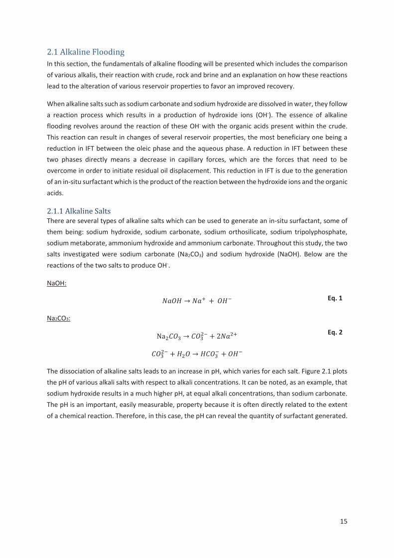
2.1.1 Alkaline Salts There are several types of alkaline salts which can be used to generate an in-situ surfactant, some of them being: sodium hydroxide, sodium carbonate, sodium orthosilicate, sodium tripolyphosphate, sodium metaborate, ammonium hydroxide and ammonium carbonate. Throughout this study, the two salts investigated were sodium carbonate (Na2CO3) and sodium hydroxide (NaOH). Below are the reactions of the two salts to produce OH-.

NaOH:

Na2CO3:

The dissociation of alkaline salts leads to an increase in pH, which varies for each salt. Figure 2.1 plots the pH of various alkali salts with respect to alkali concentrations. It can be noted, as an example, that sodium hydroxide results in a much higher pH, at equal alkali concentrations, than sodium carbonate. The pH is an important, easily measurable, property because it is often directly related to the extent of a chemical reaction. Therefore, in this case, the pH can reveal the quantity of surfactant generated.

Eq. 1

Eq. 2

16

The pH of a solution can be affected by its salinity. Hence the pH, of solutions of equal alkalinity but different ionic strengths, will be different. For instance, when the salinity of a NaOH solution of 13.2 pH is increased from 0 to 1%wt NaCl, the pH of the solution will decrease to 12.5. The sensibility at which a solution’s pH is affected by a change in salinity also varies for each salt. For example, studies have demonstrated that Na2CO3 is less sensitive as NaOH (Labrid 1991).

It is worth noting that as further alkaline salts are dissolved there’s an increase in alkalinity and an increase in salinity. Therefore, since these two properties have opposing effects, determining the optimum alkaline concentration for a flood is not so simple. Figure 2.2 shows the dynamic IFT between a crude sample and NaOH solutions at different concentrations. It can be observed that at a low NaOH concentration of 1 X 10-4 mol/L (curve 1), the IFT is not significantly altered. This is due to too little surfactant being generated at the oil/water interface. When the NaOH concentration is slightly increased to 5 X 10-4 mol/L (curve 2), the IFT reduces temporarily. This occurs because the soap being generated at the interfaces swiftly dissipates into the aqueous solution. As the NaOH concentration is increased further to 1 X 10-3 mol/L (curve 3) and 5 X 10-3 mol/L (curve 4) the IFT remains low. If the concentration is increased too much however, to 1 X 10-2 (curve 5), the IFT once again remains low only momentarily. This is due to the effects of salinity becoming dominant over the effects of alkalinity (Zhao 2002). This evidentiates that there is an optimum range of alkaline concentration for a given scenario.

Figure 2.1 Graph of pH values of alkaline solutions at different concentration at 25°C. 1,sodium hydroxide (NaOH). 2, sodium orthosilicate (Na4SiO4). 3, sodium metasilicate

(water glass or liquid glass, Na2SiO3). 4, sodium silicate pentahydrate (Na2SiO3.5H20). 5, sodium phosphate (Na3PO4.12H20). 6, sodium silicate [(Na2O)(SiO2)n, n=2 where n is the

weight ratio of SiO2 to Na2O]. 7, sodium silicate [(Na2O)(SiO2)n, n=2.4. 8, sodium carbonate (Na2CO3). 9. [sodium silicate [(Na2O)(SiO2)n, n=3.22]. 10, sodium

pyrophosphate (Na4P2O7). 11, sodium tripolyphosphate (Na5P3O10). 12, sodium bicarbonate (NaHCO3) (Sheng 2011).

17

2.1.2 Alkaline Reaction with Crude Within the crude there is an unspecified mixture of cyclopenthyl and carboxylic acids with molecular weights ranging from 120 to over 700 (Shuler 1989). These acids are grouped and defined as naphthenic acids. In order to quantify the chemical reaction, these acids are grouped and simplified to a single, highly oil-soluble pseudo-acid component (HA). When hydroxide ions are present in the aqueous solution, the acid component will donate a proton (H+) to the hydroxide ion consequently becoming ionized. The reaction of this process is described simply by the reaction below.

– pseudo-acid component in aqueous phase.

- hydrogen ion.

- Ionized acid component.

The ionized acid (A-) is a soluble anionic surfactant with a chemical structure of RCOO-. The R symbolizes an unspecified chain of carbon atoms. Conversely, only a fraction of the acids within the crude will go through this process of becoming ionized, with the other fraction remaining electronically neutral. The ionized acids, present in the aqueous phase, will bond to the electronically neutral acids, present in the oleic phase, via hydrogen bonds and in the process form a complex identified as acid soap (deZabala 1982). A schematic depicting this process can be seen in figure 2.3.

The concentration of carboxylic acids varies between crudes and plays a part in determining how much in-situ surfactant is generated. The concentration of carboxylic acids is identified by the acid number

Eq.3

Figure 2.3 Schematic of alkaline recovery process (deZabala 1982).

Figure 2.2 Dynamic IFT between a crude oil and NaOH solutions at different concentrations.

NaOH concentrations (10-3 mol/L); 1,0.1; 2,0.5; 3,1; 4,5; and 5,10 (Zhao 2002).

18

which is measured by recording the mass of potassium hydroxide (KOH) in milligrams required to neutralize one gram of the crude (Fan and Buckley 2007). Figure 2.4 plots the dynamic IFT between a 1.0% NaOH solution and gasoline oils with varying acid numbers. It can be observed that the IFT curves differ for different acid concentrations. This varing behavior conveys that an alkaline flood needs also to be tailored with respect to the crude of interest.

2.1.3 Alkaline Reaction with Rock In the schematic shown in figure 2.3, which depicts the hydroxide reactions occurring within the reservoir, it can be observed that hydroxide ions can also be consumed, via ion exchange, with ions present on the surface of the rock. For instance, it is common for hydrogen ions to be present on clay minerals. As the solution’s pH increases, the hydrogen ions will react with the hydroxide ions to produce water, lowering the pH of the solution. Alkaline can also react directly with rock minerals. For instance, alkaline floods can dissolute anyhydrate and gypsum. Ehrlich and Wygal conducted tests measuring the quantity of alkaline consumption per gram of rock occurring when an alkaline solution is placed in contact with various crushed reservoir rock samples. Figure 2.5, shows the alkaline consumption for various minerals after being exposed to a 5% NaOH solution at room temperature. It can be noted that for quartz sand, which is the rock of interest in this study, there is an “insignificant” quantity of alkaline consumption (Ehrlich and Wygal 1977).

Figure 2.4 Effect of acid number on dynamic IFT (30°C). Acid number (mg KOH/g oil): 1,00; 2,0.1; 3,0.5; 4,1.0; and 5,2.0

(Yang 1992).

Figure 2.5 Table showing alkalinity loss (meq/kg) by minerals (Ehrlich and Wygal 1977; Mohnot and Bae 1989).

19

2.1.4 Alkaline Reaction with Hard Water The alkaline can also react with ions present in the reservoir brine, most importantly divalent ions such as Ca2+ and Mg2+. When in contact with these ions, precipitate of calcium and magnesium hydroxide, carbonate and silicate may occur. The degree of permeability damage varies for different alkaline salts. Figure 2.6 shows the permeability damage, due to precipitation within the porous media, of equivalent porosity mediums and flow rates.

It can be noted that for silicate precipitates, which are generally hydrated and flocculent, the permeability damage is much more severe. While, carbonate precipitates, which are granular and less adhering on solid surfaces the permeability damage is not as severe (Cheng 1986). For the core flooding study, the alkaline agent used was Na2CO3. It is predicted that precipitation within the reservoir will not be too much of a concern.

When designing an alkaline flood it is essential to account the alkaline being consumed or lost by reacting with ions present in the brine and on the mineral surface. These reactions are unfavorable because they alter the reservoir’s lattice structure and weaken the flood’s effect at reducing the IFT. Having a weaker alkaline, such as sodium carbonate, has showed to be more preferable because due to its lower pH, the extent of these unwanted reactions will be lower. In addition sodium carbonate has shown to be less emulsifying than sodium hydroxide. This was also observed throughout the emulsion study within this work. Emulsions have the potential of having negative consequences because they tend to be highly viscous and therefore challenging to mobilize once formed. However, some conducted studies have also concluded emulsions to be favorable for recovery (Sheng 2011).

2.1.5 Alkaline Recovery Mechanisms As previously conversed, the prime recovery mechanism in an alkaline flood is the reduction in IFT that occurs due to the generation of in-situ surfactant. However, emulsification and wettability reversal have also been noted to occur during alkaline flooding and identified as contributing recovery mechanisms. The several proposed recovery mechanisms by alkaline flooding were summarized by Johnson and are stated below (Johnson 1976).

Emulsification and Entrainment

In this mechanism, the improved recovery is due to the IFT reduction. The emulsion droplets are smaller than the pore throats and will thus not affect the recovery process. The conditions for this

Figure 2.6 Effects of alkali precipitation of flow experiments with different hardness solutions.

Extent of alkali precipitation is presented by the lengths of bars and permeability reduction is presented by the lengths of bars and permeability reduction is represented by the % displaced

next to the bars (Cheng 1986).

20

mechanism are: high pH, low acid number, low salinity and emulsion droplet size being smaller than the pore throat diameter (Subkow 1942).

Emulsification and Entrapment

In this mechanism, the emulsion droplets are larger than the smaller pore throat diameters. This causes the emulsion droplets to plug the pore once it is reached, consequently retarding the flood, at that moment in space, and improving the sweep efficiency (Jennings, Johnson, and McAuliffe 1974). Therefore, in this mechanism, a reduction in IFT and the nature of the emulsions within the reservoir act as two separate recovery mechanisms. The conditions for this to occur are: a high pH, moderate acid number, low salinity and emulsion droplet size being larger than a portion of the pore throat diameters.

Wettability Reversal (oil-Wet to Water-Wet)

In this mechanism, the improved recovery is due to the change in wettability of the reservoir to more water-wet conditions. When this occurs the relative permeability curves are changed, increasing the relative permeability of the oil phase and reducing the relative permeability of the aqueous phase (Mungan 1966).

2.2 Polymer Flooding In this section the principles of polymer flooding will be presented which includes an explanation of the types of polymers, their properties and behavior within the reservoir.

Polymer flooding is the process of adding a polymer agent to the water of a waterflood, causing an increase in viscosity and, in the case of some polymers, a decrease in relative permeability of the aqueous phase. This leads to a decrease in the mobility of the fluid which increases the efficiency of the water flood by propagating the flood more uniformly (Sheng 2011).

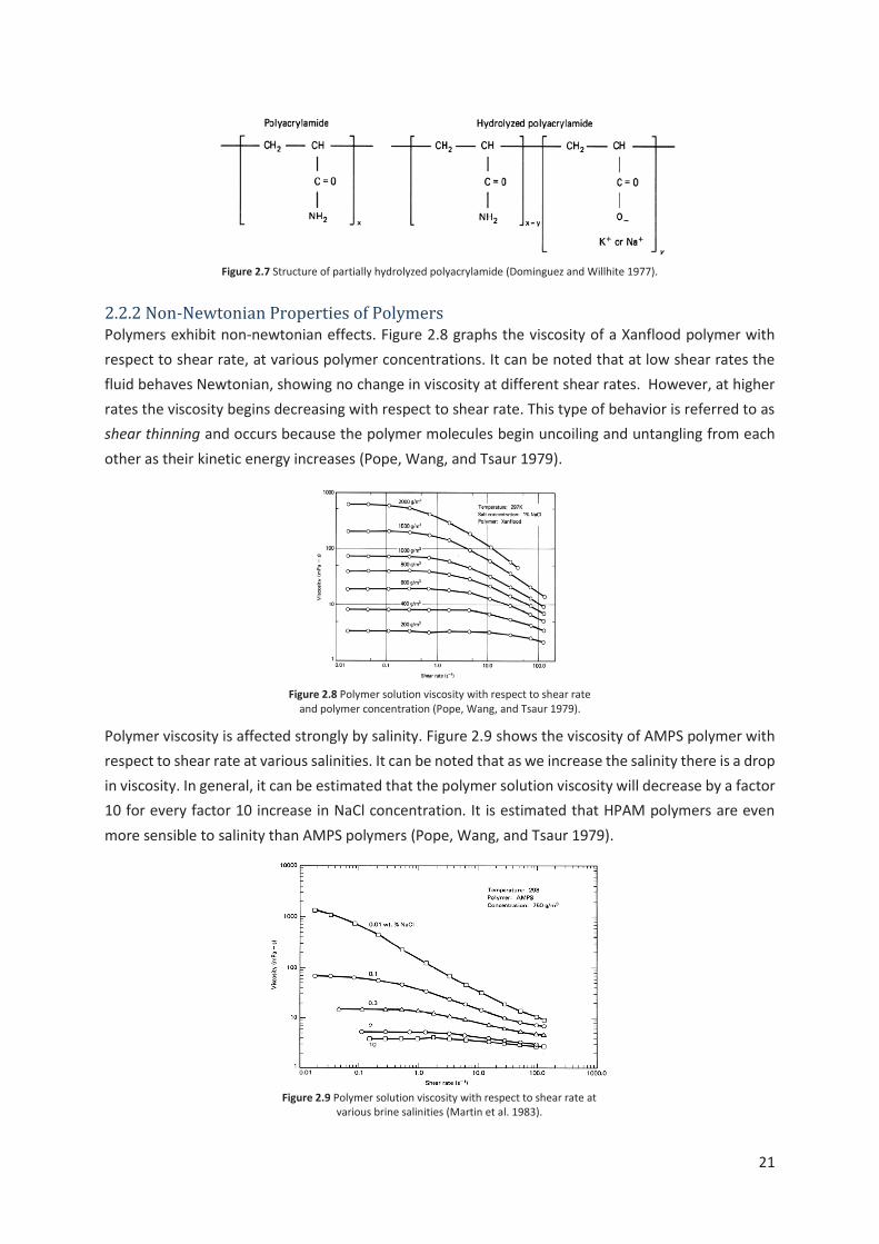
2.2.1 Polymer Types All the commercially attractive polymers used fall into two categories: polyacrylamide (HPAM) and polysaccharides (biopolymers). Throughout this study, the type of polymer used was HPAM. Figure 2.7 shows the molecular structure of a typical HPAM polymer. These polymers are called partially hydrolyzed polyacrylamides (HPAM) because a fraction of the acrylamide polymer (around 30-35%) undergo hydrolysis, consequently causing a negatively charged carboxyl group (COO-) to be scattered along the backbone chain of the polymer (Sheng 2011). This means that a HPAM molecule is negatively charged, and this accounts for many of its physical properties such as solubility, viscosity and retention. It is important to tailor and optimize the degree of hydrolysis because if it is too small the polymer will not be water soluble. If it is too large, its properties will be too sensitive to salinity and hardness (Shupe 1981).

21

2.2.2 Non-Newtonian Properties of Polymers Polymers exhibit non-newtonian effects. Figure 2.8 graphs the viscosity of a Xanflood polymer with respect to shear rate, at various polymer concentrations. It can be noted that at low shear rates the fluid behaves Newtonian, showing no change in viscosity at different shear rates. However, at higher rates the viscosity begins decreasing with respect to shear rate. This type of behavior is referred to as shear thinning and occurs because the polymer molecules begin uncoiling and untangling from each other as their kinetic energy increases (Pope, Wang, and Tsaur 1979).

Polymer viscosity is affected strongly by salinity. Figure 2.9 shows the viscosity of AMPS polymer with respect to shear rate at various salinities. It can be noted that as we increase the salinity there is a drop in viscosity. In general, it can be estimated that the polymer solution viscosity will decrease by a factor 10 for every factor 10 increase in NaCl concentration. It is estimated that HPAM polymers are even more sensible to salinity than AMPS polymers (Pope, Wang, and Tsaur 1979).

Figure 2.7 Structure of partially hydrolyzed polyacrylamide (Dominguez and Willhite 1977).

Figure 2.8 Polymer solution viscosity with respect to shear rate and polymer concentration (Pope, Wang, and Tsaur 1979).

Figure 2.9 Polymer solution viscosity with respect to shear rate at various brine salinities (Martin et al. 1983).

22

2.2.3 Polymer behavior within Porous Media Polymer Retention

Polymers experience a retention within the porous media due to adsorption onto the rock surface and trapping within small pores. Polymer retention causes a loss in polymer and therefore a decrease in its effectiveness at increasing the viscosity of the solution. The loss of polymer is a function of the type of polymer, the molecular weight of the polymer, brine salinity, brine hardness, flow rate, temperature, rock composition and pore size distribution. Polymer retention values, measured in the field, ranges from 7-150 μg polymer/cm3 of bulk volume of rock. As a rule of thumb, the desirable retention level should be below 20 μg /cm3 (Szabo 1979).

Polymer Acceleration

Polymer flooding can also show accelerating behavior through the rock media due to inaccessible pore volume (IPV). This occurs because the large polymer molecules are not able to access small pores and therefore will bypass them as the polymer propagates through the porous media. Generally this is unfavorable because it leads to an early breakthrough and a decrease in sweep efficiency. The fraction of IPV, to the whole porous volume depends on the media’s permeability, the media’s porosity, pore size distribution and polymer molecular weight (Lai 2008).

Chemical and Mechanical Degradation

Chemical and mechanical degradation cause the breakdown of polymer molecules into smaller sizes, which will reduce their function. Chemical degradation encompasses all processes such as thermal, oxidation, hydrolysis and biological. These reactions can be fast and slow. It is worth noting that the time at which a polymer stays within the reservoir is quite long, therefore even slow reactions could degrade the polymer significantly and therefore need to be considered (Lai 2008). In addition, reactions can be catalyzed by high pH, high temperatures and hardness.

2.3 Alkaline and Polymer Flooding Alkaline flooding alone has showed some challenges in being effective because it is difficult to propagate throughout the reservoir to react with sufficient volumes of crude. This is due, as mentioned previously, to alkaline being consumed along the way from ion-exchange, mineral dissolution, and precipitation. However, also due to the lack of mobility control (Sheng 2011). To remedy the lack of mobility control, it is possible to add a polymer to the solution, therefore turning it into an alkaline and polymer (AP) flood. This section serves to discuss the types of AP floods and the co-interaction between the alkaline and the polymer.

2.3.1 Types of Alkaline and Polymer Floods There are three ways of conducting a polymer and alkaline flood. The first way is to inject an alkaline flood followed by a polymer flood (A/P). The second way is to inject a polymer flood followed by an alkaline flood (P/A). The third way is to inject a flood containing both polymer and alkaline. Research has showed that the third method, injecting polymer and alkaline simultaneously, to be the most effective method of the three (Katsanis, Krumrine, and Falcone 1983). This observation can be noted

23

in figure 2.10, where the incremental recovery obtained after water flooding, from various polymer and alkaline flooding experiments, are plotted.

2.3.2 Polymer Effect on the pH Alkaline and polymer can react together, hydrolyzing the polymer. Figure 2.11 plots the pH with respect to exposure time for 1000 mg/L HPAM polymer solutions containing various concentrations of sodium carbonate. It can be noted that over time the pH decreases, demonstrating that the alkaline is indeed being consumed. This effect could be minimized by adding polymer and alkaline buffers (Sheng 1994).

2.3.3 Alkaline Effect on Polymer Viscosity The viscosity of the polymer is affected by the addition of an alkaline in two ways. As mentioned, the addition of an alkaline hydrolyzes the polymer which causes the viscosity of the solution to increase. However, the addition of an alkaline also increases the salinity of the solution. Increasing the salinity can reduce the viscosity of the flood because of the cation electric shield effect which reduces the stretch and dispersion of the polymer molecules within the solution (Sheng 2011). Therefore, with the addition of an alkaline to a polymer solution, the viscosity will either increase or decrease depending which of the two effects is dominant at a moment in time. This behavior can be noted in figure 2.12, which graphs the viscosity of a 1000 mg/L HPAM polymer solution with respect to time at various NaOH concentrations.

Figure 2.10 Comparison of residual oil recovery factors in alkaline flood, polymer flood and the various combinations of the two

(Katsanis, Krumrine, and Falcone 1983).

Figure 2.11 Graph plotting changes of pH with exposure time (Sheng 1994).

24

In figure 2.12, it can be observed that an incremental increase of NaOH leads to a general incremental increase in viscosity over a 45 day period. This occurs because at the early stages of the reaction the effects from hydrolysis are more dominant over the effects of salinity. However, in the long run, the contrary occurs. Ultimately, the addition of an alkaline will result in a decrease of the viscosity of the polymer solution (Kang 2001). This is shown in figure 2.13 where the viscosity of the HPAM with respect to shear rate is plotted at various alkaline concentrations.

2.3.4 Polymer Effect on Alkaline/Oil IFT In general it is believed that polymer has a minimal effect on IFT, however some experiments have indicated that some changes do occur because of small quantities of surfactant that are usually added to polymer agents. Experimental results demonstrated that in a polymer-alkaline system the IFT is affected differently for various alkaline salts and polymer hydrolysis (Potts and Kuehne 1988). This behavior can be noted in figure 2.14. Sodium carbonate reduced the IFT further than sodium hydroxide and an increase in polymer hydrolysis lead to greater reductions in IFT.

Figure 2.13 Alkaline effect on polymer (1000 mg/L 1275A) viscosity (Kang 2001).

Figure 2.12 NaOH-HPAM solution viscosity with respect to time. 21.5% hydrolysis, 1000 mg/L HPAM, 60°C, 3215 mg/L TDS (Sheng 1994).

25

2.3.5 Polymer Adsorption in Polymer Alkaline System A benefit from having an alkaline polymer system is a reduction in polymer adsorption and alkaline consumption. This occurs because both the alkaline and the polymer have a natural tendency to adsorb onto positively charges sites on the rock surface. When both agents are present, they will compete for the sites resulting in less consumption of each agent to when only one of the agent is present (Krumrine and Falcone 1987).

Chapter 3: Geologic Background In this chapter information regarding the Matzen field and its reservoirs in focus, including geological descriptions and production histories, are presented.

3.1 The Matzen Field The Matzen field is located 30 km northeast of Vienna, approximately situated in the middle of the Vienna basin, which is considered the most prolific and important hydrocarbon region in Austria as shown in figure 3.1 (Gruenwalder, Poellitzer, and Clemens 2007).

Figure 2.14 Effects of polymer hydrolysis, type of alkali and exposure time with crude on IFT.

3315 mg/L TDS water, °C, 0.50 mg KOH/g acid number. The NaOH concentration was 1% whereas the Na2CO3 concentration was 3%

(Sheng 1993).

Figure 3.1 General location of the Matzen Field. (Gruenwalder, Poellitzer, and Clemens 2007)

26

The field was discovered in 1949 and extensive exploration was directed by OMV to understand the nature of the field. The field consists of over 400 production units distributed in various stratigraphic beds, deposited during the middle and late Miocene Age (23-7.1 Ma) (Hölzel M. 2010). Figure 3.2 shows a stratigraphic column of the Matzen field. It can be noted, that the majority of the field’s reservoirs are composed of shallow-marine to fluvial clastic sediments deposited during the Badenian Paratethys stage (16.1-12.7 Ma).

The structure of the Matzen field can be divided into 4 regions. The first region, located in the central part of the field, is the Matzen anticline, an elongated, NE-SW trending anticline. The second region is the Matzen fault zone, a pull-apart graben in the north bounden by strike-slip faults. The third region, located in the west, is identified as the Bockfliess fault system. The fourth region, located in the south, is the Markgrafneusiedl normal fault zone. The trap mechanism of the the Matzen field are thus anticlinal structures and fault-related traps. Up to date there has been approximately 1500 wells which have been drilled in the Matzen field, which have produced 516 million bbl of oil and 1.1 tcf of gas.

3.2 Reservoir of Interest-16TH Background Information The most prolific of the Matzen’s horizons is the 16 Torton Horizon (TH). The 16TH is a reservoir of excellent quality with an average porosity of 27% and an average absolute permeability of 1190 mD. It is composed of seven layers separated by thin layers of shale deposited during brief flooding events, as shown in figure 3.3. Each layer is composed of prograding sand-rich delta front deposits and transgressive shelfal sediments (Kienberger and Fuchs 2006).

Figure 3.2 Stratigraphy of the Matzen reservoir in the Middle Miocene (Hölzel M. 2010).

27

The original oil in place (OOIP) was estimated to be 556.8 million barrels with an additional 95 billion cu-ft of free gas initially in place. Dating from 2006, 266 million STB of oil and 140 billion sc-ft of gas have been produced, which is a recovery factor of 48.5%. Further information regarding reservoir is summarized in table 3.1.

16TH Reservoir Characteristics Property Value

Average Porosity [-] 0.27 Average Permeability [mD] 1190

Original Oil in Place, OOIP [MMbbl] 556.8 Initial Gas in Place, IGIP [Bcuft] 95 Initial Water saturation, Sw [-] 0.15

Average Oil sand Net thickness [m] 17.1 Initial Gas Cap Net Thickness [-] 8.7

Oil Gravity [API] 24.8 Initial Oil Viscosity [cP] 5

Initial solution GOR [m3/m3] 45 Initial Reservoir Pressure [bars] 160

Reservoir Temperature [C] 60 Table 3.1 16TH reservoir characteristics.

Throughout the life of the reservoir water and gas injection were implemented for pressure maintenance, which have increased the life of the reservoir substantially. The production history of the reservoir is displayed in figure 3.4. It can be observed that once water injection was started, in 1968, the yearly production decline rate dropped from 8.3% to 4%. Once gas injection was started in 1995 the decline rate further reduced by 2%. The reservoir is currently producing at a rate of 2700 STB/day at a water cut of 93.5%.Studies estimate that 85% of that production is due to the implementation of water and gas injection.

Figure 3.3 Transgression of the Matzen Sand (16th – Main Pool), onlapping on older sediments (Kienberger and Fuchs 2006).

28

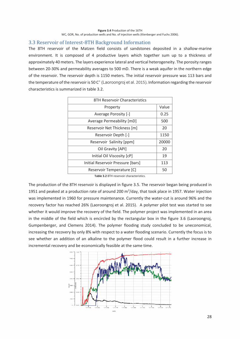
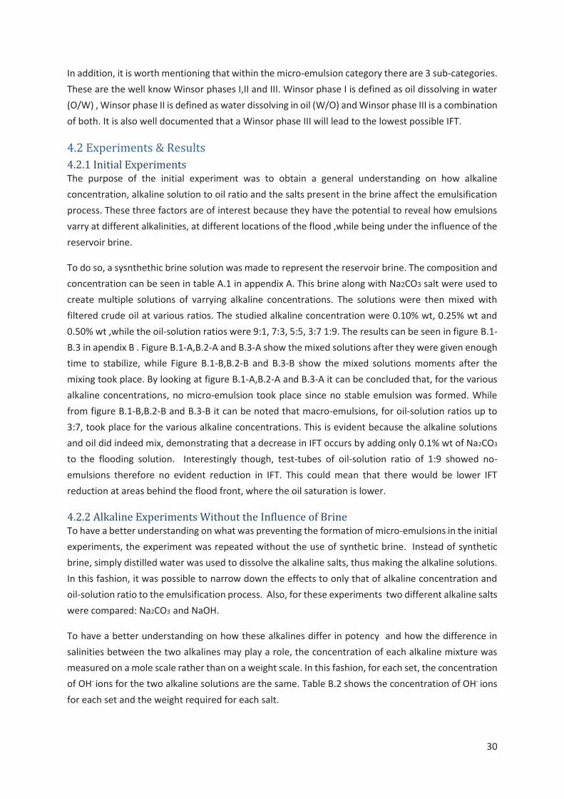
3.3 Reservoir of Interest-8TH Background Information The 8TH reservoir of the Matzen field consists of sandstones deposited in a shallow-marine environment. It is composed of 4 productive layers which together sum up to a thickness of approximately 40 meters. The layers experience lateral and vertical heterogeneity. The porosity ranges between 20-30% and permeability averages to 500 mD. There is a weak aquifer in the northern edge of the reservoir. The reservoir depth is 1150 meters. The initial reservoir pressure was 113 bars and the temperature of the reservoir is 50 C° (Laoroongroj et al. 2015). Information regarding the reservoir characteristics is summarized in table 3.2.

8TH Reservoir Characteristics Property Value

Average Porosity [-] 0.25 Average Permeability [mD] 500 Reservoir Net Thickness [m] 20

Reservoir Depth [-] 1150 Reservoir Salinity [ppm] 20000

Oil Gravity [API] 20 Initial Oil Viscosity [cP] 19

Initial Reservoir Pressure [bars] 113 Reservoir Temperature [C] 50

Table 3.2 8TH reservoir characteristics.

The production of the 8TH reservoir is displayed in figure 3.5. The reservoir began being produced in 1951 and peaked at a production rate of around 200 m3/day, that took place in 1957. Water injection was implemented in 1960 for pressure maintenance. Currently the water-cut is around 96% and the recovery factor has reached 26% (Laoroongroj et al. 2015). A polymer pilot test was started to see whether it would improve the recovery of the field. The polymer project was implemented in an area in the middle of the field which is encircled by the rectangular box in the figure 3.6 (Laoroongroj, Gumpenberger, and Clemens 2014). The polymer flooding study concluded to be uneconomical, increasing the recovery by only 8% with respect to a water flooding scenario. Currently the focus is to see whether an addition of an alkaline to the polymer flood could result in a further increase in incremental recovery and be economically feasible at the same time.

Figure 3.4 Production of the 16TH WC, GOR, No. of production wells and No. of injection wells (Kienberger and Fuchs 2006).

29

Chapter 4: Emulsion Study As mentioned in the introduction, within this master thesis an emulsion and a core flooding study were conducted to examin whether AP flooding is a suitable EOR method for the 8TH and 16TH reservoirs of the Matzen field.

4.1 Introduction The purpose of this chapter is to present the emulsion study, which focuses on understanding the circumstances at which a micro-emulsion takes place between alkaline solutions and crude oil coming from the 8TH Reservoir of the Matzen field in Austria. As mentioned in the literature review, emulsification can be advantageous by acting as a recovery mechanism, or it can be disadvantageous by becoming too viscous to displace. In this emulsion study, however, the formation of an emulsion was observed and used as an indication that a low IFT is present. Therefore, noting at which conditions a micro-emulsion forms can be beneficiary to calibrate an alkaline flood to optimum conditions.

In this study, varrying alkaline solutions and crude samples were mixed into test-tubes. The mixtures were observed and categorized into 1 of 3 possible categories: macro-emulsions, micro-emulsions and no-emulsions. A micro-emulsion differs from a macro-emulsion by its ability to be in a thermodynamically stable state. It is possible to distinguish a macro-emulsion from a micro-emulsion by seeing if the emulsion decomposes after some time. A no-emulsion solution means that no evidence of emulsification was noted to hint a reduction in IFT. To distinguish and make evident of these 3 categories, 2 photographs were taken for each experiment. The first photograph was taken moments after mixing and the second photograph was taken 2-3 days afterwards. For a micro-emulsion, since the emulsion is stable, its 2 photographs will be similar. For a macro-emulsion, since the emulsion is unstable, its two photographs will be different showing an emulsion in the first photograph and two separate phases in the second photograph. For a no-emulsion its two photos will be the same, showing two separate phases in both photos.

Figure 3.5 Production of the 8TH Oil (black) and liquid (green), water injection is shown in blue and the water cut in red

(Laoroongroj et al. 2015).

Figure 3.6 Top structure map of the 8TH reservoir. Blue dots indicate injectors, green dots producers. The pilor area in shown

by the red square (Laoroongroj, Gumpenberger, and Clemens 2014).

30

In addition, it is worth mentioning that within the micro-emulsion category there are 3 sub-categories. These are the well know Winsor phases I,II and III. Winsor phase I is defined as oil dissolving in water (O/W) , Winsor phase II is defined as water dissolving in oil (W/O) and Winsor phase III is a combination of both. It is also well documented that a Winsor phase III will lead to the lowest possible IFT.

4.2 Experiments & Results 4.2.1 Initial Experiments The purpose of the initial experiment was to obtain a general understanding on how alkaline concentration, alkaline solution to oil ratio and the salts present in the brine affect the emulsification process. These three factors are of interest because they have the potential to reveal how emulsions varry at different alkalinities, at different locations of the flood ,while being under the influence of the reservoir brine.

To do so, a sysnthethic brine solution was made to represent the reservoir brine. The composition and concentration can be seen in table A.1 in appendix A. This brine along with Na2CO3 salt were used to create multiple solutions of varrying alkaline concentrations. The solutions were then mixed with filtered crude oil at various ratios. The studied alkaline concentration were 0.10% wt, 0.25% wt and 0.50% wt ,while the oil-solution ratios were 9:1, 7:3, 5:5, 3:7 1:9. The results can be seen in figure B.1-B.3 in apendix B . Figure B.1-A,B.2-A and B.3-A show the mixed solutions after they were given enough time to stabilize, while Figure B.1-B,B.2-B and B.3-B show the mixed solutions moments after the mixing took place. By looking at figure B.1-A,B.2-A and B.3-A it can be concluded that, for the various alkaline concentrations, no micro-emulsion took place since no stable emulsion was formed. While from figure B.1-B,B.2-B and B.3-B it can be noted that macro-emulsions, for oil-solution ratios up to 3:7, took place for the various alkaline concentrations. This is evident because the alkaline solutions and oil did indeed mix, demonstrating that a decrease in IFT occurs by adding only 0.1% wt of Na2CO3 to the flooding solution. Interestingly though, test-tubes of oil-solution ratio of 1:9 showed no-emulsions therefore no evident reduction in IFT. This could mean that there would be lower IFT reduction at areas behind the flood front, where the oil saturation is lower.

4.2.2 Alkaline Experiments Without the Influence of Brine To have a better understanding on what was preventing the formation of micro-emulsions in the initial experiments, the experiment was repeated without the use of synthetic brine. Instead of synthetic brine, simply distilled water was used to dissolve the alkaline salts, thus making the alkaline solutions. In this fashion, it was possible to narrow down the effects to only that of alkaline concentration and oil-solution ratio to the emulsification process. Also, for these experiments two different alkaline salts were compared: Na2CO3 and NaOH.

To have a better understanding on how these alkalines differ in potency and how the difference in salinities between the two alkalines may play a role, the concentration of each alkaline mixture was measured on a mole scale rather than on a weight scale. In this fashion, for each set, the concentration of OH- ions for the two alkaline solutions are the same. Table B.2 shows the concentration of OH- ions for each set and the weight required for each salt.

31

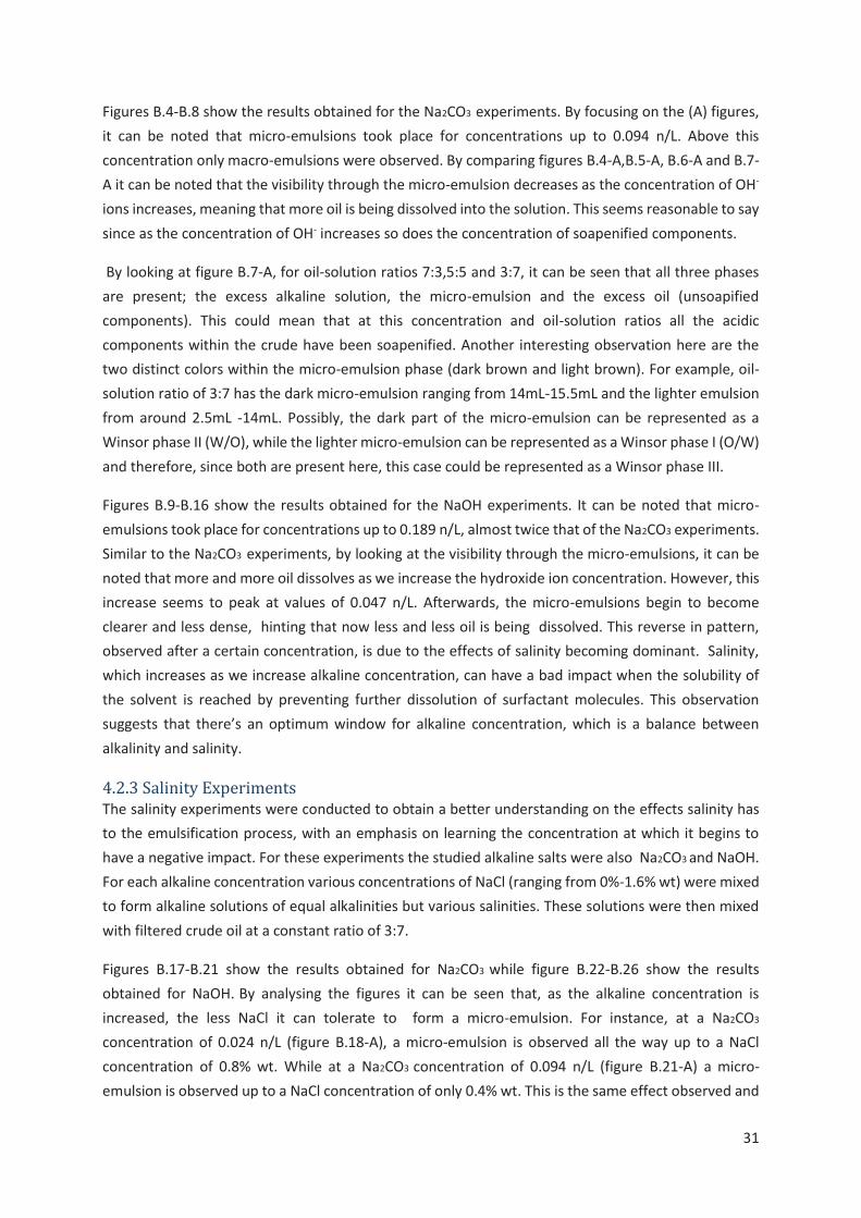
Figures B.4-B.8 show the results obtained for the Na2CO3 experiments. By focusing on the (A) figures, it can be noted that micro-emulsions took place for concentrations up to 0.094 n/L. Above this concentration only macro-emulsions were observed. By comparing figures B.4-A,B.5-A, B.6-A and B.7-A it can be noted that the visibility through the micro-emulsion decreases as the concentration of OH- ions increases, meaning that more oil is being dissolved into the solution. This seems reasonable to say since as the concentration of OH- increases so does the concentration of soapenified components.

By looking at figure B.7-A, for oil-solution ratios 7:3,5:5 and 3:7, it can be seen that all three phases are present; the excess alkaline solution, the micro-emulsion and the excess oil (unsoapified components). This could mean that at this concentration and oil-solution ratios all the acidic components within the crude have been soapenified. Another interesting observation here are the two distinct colors within the micro-emulsion phase (dark brown and light brown). For example, oil-solution ratio of 3:7 has the dark micro-emulsion ranging from 14mL-15.5mL and the lighter emulsion from around 2.5mL -14mL. Possibly, the dark part of the micro-emulsion can be represented as a Winsor phase II (W/O), while the lighter micro-emulsion can be represented as a Winsor phase I (O/W) and therefore, since both are present here, this case could be represented as a Winsor phase III.

Figures B.9-B.16 show the results obtained for the NaOH experiments. It can be noted that micro-emulsions took place for concentrations up to 0.189 n/L, almost twice that of the Na2CO3 experiments. Similar to the Na2CO3 experiments, by looking at the visibility through the micro-emulsions, it can be noted that more and more oil dissolves as we increase the hydroxide ion concentration. However, this increase seems to peak at values of 0.047 n/L. Afterwards, the micro-emulsions begin to become clearer and less dense, hinting that now less and less oil is being dissolved. This reverse in pattern, observed after a certain concentration, is due to the effects of salinity becoming dominant. Salinity, which increases as we increase alkaline concentration, can have a bad impact when the solubility of the solvent is reached by preventing further dissolution of surfactant molecules. This observation suggests that there’s an optimum window for alkaline concentration, which is a balance between alkalinity and salinity.

4.2.3 Salinity Experiments The salinity experiments were conducted to obtain a better understanding on the effects salinity has to the emulsification process, with an emphasis on learning the concentration at which it begins to have a negative impact. For these experiments the studied alkaline salts were also Na2CO3 and NaOH. For each alkaline concentration various concentrations of NaCl (ranging from 0%-1.6% wt) were mixed to form alkaline solutions of equal alkalinities but various salinities. These solutions were then mixed with filtered crude oil at a constant ratio of 3:7.

Figures B.17-B.21 show the results obtained for Na2CO3 while figure B.22-B.26 show the results obtained for NaOH. By analysing the figures it can be seen that, as the alkaline concentration is increased, the less NaCl it can tolerate to form a micro-emulsion. For instance, at a Na2CO3

concentration of 0.024 n/L (figure B.18-A), a micro-emulsion is observed all the way up to a NaCl concentration of 0.8% wt. While at a Na2CO3 concentration of 0.094 n/L (figure B.21-A) a micro-emulsion is observed up to a NaCl concentration of only 0.4% wt. This is the same effect observed and

32

described in the previous experiments where, due to the salinity increase, the lower the capacity of surfactant molecules that can be dissolved in the solution.

One thing to note here is that the salinity at which micro-emulsions stop forming is significantly lower than the salinity of the reservoir. tables B.2 and B.3 show the salinity of the salinty experiments. In each table the salinity at which a micro-emulsion is no longer observed is bolded. This max salinity ranges from 10,000 ppm to 14,000 ppm. This is much lower than the reservoir brine salinity which is around 25,000 ppm. Therefore, it is fair to assume that unless the salinity of the reservoir is softened or an additional surfactant is added to the EOR flood, no micro-emulsion will form at these reservoir conditions with only an alkaline present in the flood.

An interesting observation, that is also worth mentioning, can be spotted in figure B.17-A. It can be seen that as we increase the NaCl concentration from 0% to 0.2% there is actually an improvement, since the micro-emulsion’s density increases. This is an interesting observation which is only noted at low salinities.

Another observation to point out is that as the salinity increases, there seems to be changes in proportions of the Winsor I and Winsor II phases within the micro-emulsion phase. This can be well seen in figure B.19-A. It can be seen as we go from 0% to 0.6% NaCl concentration the smaller the Winsor phase I becomes and the larger the Winsor phase II becomes. This type of observation has been documented before in literature stating that, as we increase the salinity, the micro-emulsion phase goes from a Winsor phase I to a Winsor phase III to a Winsor phase II.

4.2.4 EDTA Experiments The EDTA experiments were conducted to study how divalent ions, present in the reservoir brine, influence the emulsification process. It is well known that calcium ions can hinter the effectiveness of an alkaline flood by consuming the alkaline and causing precipitation. For instance, recall that when Na2CO3 is used as the alkaline salt, it is the carbonate ion´s (CO3 -2) reaction with water which is forming the OH-. When calcium ions are present in the solution however, the carbonate ions will react with the calcium ions to precipiate calcium carbonate (The reaction is stated below). This is detrimental because firstly it reduces alkalinity by consuming CO3 -2 ions and secondly it causes precipitation that could damage the pumps.

To prevent this, an EDTA agent (Ttitriplex III salt was used) can be introduced to the solution to sequester the calcium ions, rendering them inactive. The EDTA´s reaction with the calcium ions is stated below.

However, although adding the EDTA salt sequesters the calcium ions, it does also increase the saliniy. And we have seen that too high of a salinity can negatively impact emulsification. Therefore, is is questionable whether the EDTA agent will be effective or not. For this reason, in this experiment, various EDTA concentrations were studied which are stated in table B.4. Each EDTA concentration is

Eq. 4

Eq. 5

33

represented as a multiplication factor of the exact concentration required to neutralize al the calicum ion within the solution. For example, a multiplication factor of X 0.5 means that, at this EDTA concentration, only half the calcium ions can be sequestered. A multiplication factor of X 1.0 means that, at this EDTA concentration, all of the calciums ions are sequestered. A multiplication factor of X 2.0 means that there is twice the amount of EDTA needed to sequester all of the calcium, hence half of it will remain in the solution as excess.

For the EDTA experiments various solutions were formed of: varrying alkaline concentration, varrying EDTA concentration and a CaCl2 concentration of 1.15 g/L (the concentration of the synthetic brine). These solutions were then mixed with filtered crude oil at a ratio of 3:7.

Figures B.27-B.30 show the results obtained for the Na2CO3 solutions while figure B.31-B.34 show the results obtained for the NaOH solutions. The results are quite interesting and counter-intuitive. For instance, for Na2CO3 solutions, emulsification is only minorly affected by the presence of calcium. The negative effects of calcium are only noted at low Na2CO3 concentrations (0.009 n/L and 0.024 n/L) and can be observed in figure B.27 and B.28. At these two concentrations all test tubes showed no-emulsions because too much of the alkaline is consumed by the calcium, preventing emulsification. However, at higher Na2CO3 concentrations, micro-emulsions form even with little to no EDTA in the solutions. This is noted by looking at figure B.29 and B.30, where micro-emulsions are present at EDTA factors of X 0.0 and X 0.5.

Quite different results are obtained for the NaOH experiments. Unlike Na2CO3, the NaOH solutions seem very sensible to the presence of calcium. This can be noted from figures B.31-B.34, where for the various NaOH concentratrions, unless all the calcium ions are sequestered (factor of X 1.0 or bigger) , there is absolutely no micro-emulsion forming.

4.3 Concluding Remarks In summary, the goal of the study was to build a better understanding on how emulsions work and the conditions at which they form for the crude coming from 8TH reservoir of the Matzen field in Austria. The initial experiments were conducted to see how the emulsions varry at different concentrations and oil-solutions ratios all under the influence of the reservoir brine. It was found that only macro-emulsions form at those conditions and that at low oil-solution ratios no-emulsions form. From the salinity experiments it was found that no micro-emulsion would form at salinities above 15,000 ppm, which is of a concern because the salinity of the reservoir is around 25,000 ppm. From the EDTA experiments, it was found that Na2CO3 is very tolerant to calcium ions, however without the EDTA agent precipitation occurs. The opposite effects were observed for NaOH, where it is quite intolerable to calcium ions and no precipitation occurs.

Chapter 5: Core Flood Study 5.1 Introduction The purpose of this chapter is to present the core flooding study which focused on understanding how alkaline and polymer individually and conjointly affect the recovery process. While also testing various flood compositions to observe which would be the most effective. This was done by conducting a series of aged core floods experiments and measuring the following properties: oil rate, water rate, pH, tracer

34

concentration and polymer concentration. Throughout this chapter the flood design, experiment preparation, experiment procedure, and experiment results are explained.

5.2 Flood Design Throughout this study four categories of flooding experiments were conducted, identified as: Base Scenario, Alkaline Scenario, Polymer Scenario and Alkaline & Polymer Scenario. The purpose of the Base Scenario was to observe how much recovery is obtained solely by waterflooding. The purpose of the Alkaline Scenario was to observe how much recovery is obtained with only alkaline flooding. The purpose of the Polymer Scenario was to observe how much recovery is obtained with only polymer flooding. The purpose of the Alkaline & Polymer Scenario was to observe how much recovery is obtained when both alkaline and polymer are injected simultaneously.

For every flood several properties were kept constant such as: polymer and alkaline agent and concentration, slug size and injection rate. Table 5.1 shows the values of the mentioned properties. The base fluid for the floods was the synthetic brine, its composition can be seen in table A.1 in appendix A.

Constant Flood Properties Properties Values

Alkaline Salt Na2CO3 Alkaline concentration [wt%] 1

Polymer Salt FLOPAM 3630 S Polymer Concentration [ppm] 800

Slug Size [P.V] 0.8 Injection Rate [mL/min] 1

Table 5.1 Constant flood properties.

Within the Alkaline Scenario and Alkaline & Polymer Scenario, due to the presence of CO3 -2 and calcium ions, it was necessary to modify the floods in order to prevent precipitation from occurring. It is of vital importance to prevent precipitation from occurring prior to injection because the precipitates could damage the pumps. Within the study two methods preventing precipitation were investigated. The first method involved adding an EDTA agent (Triplex III) to sequester the calcium ions, rendering them inactive.The second method was to remove the calcium chloride (CaCl2) salt from the solution, equivalent to softening the brine, prior to adding the alkaline salt. These two methods were both tested for each flood containing an alkaline agent to learn which of the two is most effective.

5.2.1 Flood Compositions Base Scenario

Table 5.2 shows the composition for the Base Scenario floods. The composition is solely composed of the synthetic brine salts.

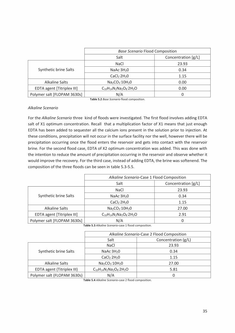
35

Base Scenario Flood Composition Salt Concentration [g/L]

Synthetic brine Salts NaCl 23.93

NaAc.3H20 0.34 CaCl2.2H20 1.15

Alkaline Salts Na2CO3.10H20 0.00

EDTA agent [Titriplex III] C10H14N2Na2O8.2H2O 0.00

Polymer salt [FLOPAM 3630s] N/A 0 Table 5.2 Base Scenario flood composition.

Alkaline Scenario

For the Alkaline Scenario three kind of floods were investigated. The first flood involves adding EDTA salt of X1 optimum concentration. Recall that a multiplication factor of X1 means that just enough EDTA has been added to sequester all the calcium ions present in the solution prior to injection. At these conditions, precipitation will not occur in the surface facility nor the well, however there will be precipitation occurring once the flood enters the reservoir and gets into contact with the reservoir brine. For the second flood case, EDTA of X2 optimum concentration was added. This was done with the intention to reduce the amount of precipitation occurring in the reservoir and observe whether it would improve the recovery. For the third case, instead of adding EDTA, the brine was softenend. The composition of the three floods can be seen in table 5.3-5.5.

Alkaline Scenario-Case 1 Flood Composition Salt Concentration [g/L]

Synthetic brine Salts NaCl 23.93

NaAc.3H20 0.34 CaCl2.2H20 1.15

Alkaline Salts Na2CO3.10H20 27.00

EDTA agent [Titriplex III] C10H14N2Na2O8.2H2O 2.91

Polymer salt [FLOPAM 3630s] N/A 0 Table 5.3 Alkaline Scenario-case 1 flood composition.

Alkaline Scenario-Case 2 Flood Composition Salt Concentration (g/L)

Synthetic brine Salts NaCl 23.93

NaAc.3H20 0.34 CaCl2.2H20 1.15

Alkaline Salts Na2CO3.10H20 27.00

EDTA agent (Titriplex III) C10H14N2Na2O8.2H2O 5.81

Polymer salt (FLOPAM 3630s) N/A 0 Table 5.4 Alkaline Scenario-case 2 flood composition.

36

Alkaline Scenario-Case 3 Flood Composition Salt Concentration (g/L)

Synthetic brine Salts NaCl 23.93

NaAc.3H20 0.34 CaCl2.2H20 0.00

Alkaline Salts Na2CO3.10H20 27.00

EDTA agent (Titriplex III) C10H14N2Na2O8.2H2O 0.00

Polymer salt (FLOPAM 3630s) N/A 0 Table 5.5 Alkaline Scenario-case 3 flood composition.

Polymer Scenerio

For the Polymer Scenario the composition consisted of the polymer agent and the synthetic brine. The composition can be seen in table 5.6.

Polymer Scenario Flood Composition Salt Concentration [g/L]

Synthetic brine Salts NaCl 23.93

NaAc.3H20 0.34 CaCl2.2H20 1.15

Alkaline Salts Na2CO3.10H20 0.00

EDTA agent [Titriplex III] C10H14N2Na2O8.2H2O 0.00

Polymer salt [FLOPAM 3630s] N/A 0.8 Table 5.6 Polymer Scenario flood composition.

Alkaline & Polymer Scenario

For the Alkaline & Polymer Scenario two types of floods were conducted. In the first case the EDTA agent was added at X1 optimum concentration and for the second case the brine was softened. The composition of the floods can be seen in table 5.7-5.8. The design for all the floods is summarized in figure 5.1.

Alkaline & Polymer Scenario -Case 1 Flood Composition Salt Concentration [g/L]

Synthetic brine Salts NaCl 23.93

NaAc.3H20 0.34 CaCl2.2H20 1.15

Alkaline Salts Na2CO3.10H20 27.00

EDTA agent [Titriplex III] C10H14N2Na2O8.2H2O 2.91

Polymer salt [FLOPAM 3630s] N/A 0.8 Table 5.7 Alkaline & Polymer Scenario -case 1 flood composition.

37

Alkaline & Polymer Scenario -Case 2 Flood Composition Salt Concentration [g/L]

Synthetic brine Salts NaCl 23.93

NaAc.3H20 0.34 CaCl2.2H20 0.00

Alkaline Salts Na2CO3.10H20 27.00

EDTA agent [Titriplex III] C10H14N2Na2O8.2H2O 0.00

Polymer salt [FLOPAM 3630s] N/A 0.8 Table 5.8 Alkaline & Polymer Scenario -case 2 flood composition.

5.3 Experiment Preparation & Procedure In order to be able to conduct the core flood experiments it was first necessary to prepare a series of core plugs to resemble the conditions of the 8TH reservoir of the Matzen field. In this section the material, equipment and procedure used to prepare the samples and conduct the experiments are presented.

Figure 5.1 Summary of flood compositions.

38

5.3.1 Conventional Core Analysis For this study, outcrop Berea sandstone samples of the 14TH horizon were used. Figure 5.2 shows the initial state of the cores. Conventional Core Analysis (CCA) for each core was conducted to measure the following properties: bulk volume (BV), absolute permeability (kabs), pore volume (PV) and porosity (Ø).

The bulk volumes were measured using the mercury bath method. A picture of the experiment can be seen in figure 5.3. In this technique the cores are submerged into a bath of mercury and the increase in the bath’s weight is recorded. To calculated the bulk volume the measured weight increase is divided by the density of mercury.

The pore volumes were measured using a helium porosimeter. A picture of the experimental set-up is shown in figure 5.4. The methodology relies on recording the pressure change occuring when the pressurized chamber’s volume, housing the core, is increased. Then applying Boyle’s law to calculate the pore volume.

Force source

scale

Core Chambers

Figure 5.2 Outcrop Beare sandstone core samples used.

Figure 5.3 Merucry bath experiment to measure core bulk volume.

Figure 5.4 Porosimeter equipment used to measure pore volume.

39

The absolute permeability of the cores were measured by using a helium permeameter. A picture of the experimental set-up is seen in figure 5.5. The methodology relies on recording the pressure drop across the core sample at a given flow rate, then using Darcy’s law to calculate the permeability. A correction factor was also applied to account for the gas slippage effect. The CCA property values for each core can be see in table A.2 in appendix A.

5.3.2 Core Sleeving After the CCA, the cores were glued to fiberglass sleeves, isolating their sides. In this fashion fluids would only be able to enter and leave the cores from their tops and bottoms. The first step was to put some glue onto the cores, as shown in figure 5.6 (this was done to fascilatate centering the cores in the sleeve). Afterwards, the cores were placed into the sleeves and glue was poured between the sleeve and the core, glueing them together. Figure 5.7 shows the final result. After the glueing process was complete the permeability of the cores were remeasured to verify that the glue didn’t cause any significant formation damage.

Core Chamber

glue on the core samples

glue between the core and the sleeve

fiberglass sleeves

Figure 5.5 Permeamter equipment used to measure absolute permeability.

Figure 5.6 Glueing process of the cores.

40

5.3.3 Core Saturation Process Once the cores were sleeved it was possible to begin the saturation process. The cores were first placed into a bath of the synthetic brine, the composition of the brine can be seen in table A.1. The bath was depressurized in order to fully degas the core samples. Figure 5.8 shows an image of the process.

Afterwards, stock tank oil coming from the 8TH reservoir of the Matzen field was degassed and filtered, a figure of the process can be seen in figure 5.9. The viscosity and density of the crude as a function of temperature were also measured, the results can be seen in figure A.1.

Filter

Depressurized volume

Depressurized bath container.

Cores bathing in synthethic brine

Figure 5.7 Final result of glueeing process.

Figure 5.8 Cores being bathed in synthethic brine at low pressure.

41

The cores were then flooded with the stock tank oil, at a rate of 1mL/min, at a temperature set to 50°C. A figure of the experimental set-up can be seen in figure 5.10. The oil was flooded until a stable pressure was observed ,and no more water production was obtained. The irreducible water saturation (Swir) and OOIP of the cores were then calculated, the vaues can be seen in table A.4. Table A.3 contains the relevant information (i.e fluid densities) needed for the calculations. The calculation steps can be seen in C.1 in appendix C.

Once all the cores were saturated with crude they were placed into a bath of the crude to age for a period of one month. This was done in order to change the wettability to mixed-wet conditions, which is the wettability of the reservoir.

5.3.4 Core Flooding Procedure In this section the experiment procedure for the flooding experiments is explained. The flooding experiments were conducted in a thermostatic bath set at 50 °C.

The cores were initially flooded with simulated live oil to replace the stock tank oil present in the cores throughout the aging process.The simulated live oil consists of a mixture of fresh stock tank oil and special benzene. The special benzene was added to dilute the crude so that it mimics the viscosity of the crude at reservoir conditions. As a reminder, the crude´s viscosity is higher at stock tank conditions than at reservoir conditions because much of its gas has evolved out of the solution. Experimentally, it was derived that the volumetric fraction of special benzene needed, to match a viscosity of 20 cp at 50°C, is 9.61%. A phase behavior experiment was then conducted to test whether the special benzene would significantly affect the emulsification process, thus the IFT reduction. To do so, the simulated live oil and crude oil were mixed at various ratios with a 1% Na2CO3 wt alkaline solution. The oil-solution ratios studied were 9:1, 7:3, 5:5, 3:7 1:9. Figure 5.11 shows the mixtures after they were given a couple of days to stabilize, very little difference amonst the mixtures is observed.

Pressure transducers

Scale recording production rate

Core holder

Injection line

Figure 5.9 Stock tank oil of the 8TH reservoir being filtered and degassed.

Figure 5.10 Experimental set-up for drainage flooding process.

42

The simulated live oil was injected into the core sample at a slow rate of 0.5 mL/min until a stable pressure differential was obtained. Afterwards the core was injected with 1.2 PV of synthetic brine. This was done to bring the core to current reservoir conditions. Afterwards 0.8 PV of the EOR flood was injected followed by synthetic brine. The synthetic brine was injected until no more oil recovery was observed. Below is a summary of the flooding procedure and an image of the experimental set-up can be seen in figure 5.12.

• Flood core with simulated live oil at 0.5 mL/min until a stable pressure profile is observed. (Fluid tanks and cores were immersed into a thermo-static bath set at 50°C).

• Flood core with synthetic brine at 1.0 mL/min for a total volume of 1.2 PV.

• Inject core with flood at 1.0 mL/min for a total volume of 0.8 PV.

• Inject core with synthetic brine at 1.0 mL/min until no more oil production is observed.

5.3.5 Data Gathering Procedure For the core flooding experiments the following important properties of the effluent were recorded and studied: oil and water rate, tracer concentration, poymer concentration and pH. In this section the methods used to measure the data are explained.

Oil & Water Rate

Live oil cell

Core cell Thermostatic bath

EOR fluid cell

Figure 5.11 Phase experiment for live oil.

Figure 5.12 Core flood experiment set-up.

43

Throughout the core flooding experiments various data gathering procedures were utilized for the oil and water rates. Initially, a separator with a solenoid magnetic valve was installed to the production flow line, the set-up can be seen in figure 5.13. The separator separates the oil from the aqueous phase and redirects the fluids into two different flow lines. The oil and water flow lines then exhaust their fluids onto separate mass scales, which automatically record the cumulative mass of each phase at a chosen time step.

The separator with the solenoid magnetic valve showed to be ineffective due to a lack in sensitivity. Due to this technical problem, after some experiments, the separator was removed and the flow rates were simply recorded manually. This was done by gathering the production fluids into test tubes. Each test tube consists of 1 minute’s worth of production fluid. After the experiment, the volume of the oil and the aqueous phase were measured by reading them directly from the test tube’s measurement scale. Unfortunately, the test tubes available were too large to be able to read the volume of each phase accurately.

Later through the project, an ingenious new separator was designed and assembled by Leopold Huber, which proved to be quite effective and accurate. Figure 5.14 shows a picture of the experimental set-up. The production fluid line is connected to the bottom end of a burette, initially filled with brine. The

Scale

Production line

Oil line

Water line

solenoid magnetic valve

Seperator

Figure 5.13 separator with a solenoid magnetic valve.

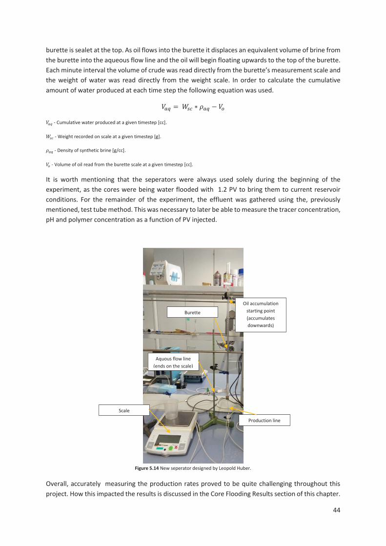
44

burette is sealet at the top. As oil flows into the burette it displaces an equivalent volume of brine from the burette into the aqueous flow line and the oil will begin floating upwards to the top of the burette. Each minute interval the volume of crude was read directly from the burette’s measurement scale and the weight of water was read directly from the weight scale. In order to calculate the cumulative amount of water produced at each time step the following equation was used.

- Cumulative water produced at a given timestep [cc].

- Weight recorded on scale at a given timestep [g].

- Density of synthetic brine [g/cc].

- Volume of oil read from the burette scale at a given timestep [cc].

It is worth mentioning that the seperators were always used solely during the beginning of the experiment, as the cores were being water flooded with 1.2 PV to bring them to current reservoir conditions. For the remainder of the experiment, the effluent was gathered using the, previously mentioned, test tube method. This was necessary to later be able to measure the tracer concentration, pH and polymer concentration as a function of PV injected.

Overall, accurately measuring the production rates proved to be quite challenging throughout this project. How this impacted the results is discussed in the Core Flooding Results section of this chapter.

Aquous flow line (ends on the scale)

Scale

Burette

Production line

Oil accumulation starting point (accumulates downwards)

Figure 5.14 New seperator designed by Leopold Huber.

45

Tracer Concentration, Polymer Concentration & pH

The tracer concentration and polymer concentration of the effluent were measured by using ion chromotographers ,while the pH was recorded using pH strips. As mentioned, after water flooding the cores with 1.2 P.V, the production was collected in 1 mL intervals. The three properties were measured for each 1 mL sample.

5.3 Core Flooding Results In this section the results of the core flooding experiments are presented. A total of 15 cores were flooded. Table 5.9 shows the flood composition for each core. The data values for the properties recorded for each core can be obtained from the excel file coreFloodingResults.xslx.

46

EOR Floods for each Core

Case Core Number

Synthetic Brine

Softened Brine (no

CaCl2)

EDTA X0

EDTA X1

EDTA X2

Alkaline Concentration Na2CO3 0% wt

Alkaline Concentration

Na2CO3 1% wt

Polymer 0 ppm

FLOPAM 3630 S Polymer 800

ppm

Base Scenario 14-358 X X X X 14-348 X X X X

Alkaline Scenario-Case 1 14-338 X X X X 14-350 X X X X

Alkaline Scenario-Case 2 14-334 X X X X

Alkaline Scenario-Case 3 14-346 X X X X 14-337 X X X X

Polymer Scenario 14-336 X X X X 14-339 14-344 X X X X

Alkaline & Polymer Scenario-Case 1

14-360 X X X X 14-357 X X X X

Alkaline & Polymer Scenario-Case 2

14-347 X X X X 14-351 X X X X 14-340 X X X X

Table 5.9 EOR flood composition for each core.

47

5.3.1 Recovery Curves To better visualize and compare the success of each flood composition, their cumulative recovery factors with respect to pore volumes injected were calculated and plotted. As discussed in section 5.3.5 (Data Gathering Procedure), there were some technical issues to accurately record the production rates. Some calculation steps were conducted to minimize the error obtained, which can be seen in section C.2 in appendix C. By applying these calculations it was possible to accurately measure the recovery factor at the end of the experiments, but not the recovery factors throughout the experiments. As a result of this, for some experiments, the shape of the recovery curves are unreliable which will be pin pointed as they are presented.

Throughout the study, it was noted that there were varying degrees of inconsistency in the ultimate recovery factor recorded for a given flood composition. To quantify the precision of the results, the average ultimate recovery factor and standard deviation (σ) for each flood composition was calculated. The results can be seen in table 5.10.

Average Total Recovery Data Scenarios [-] Average R.F [-] Standard Deviation [-]

Base Scenario 0.49 0.04 Alkaline Scenario 0.62 0.03

Alkaline Scenario-Case 2 0.69 0.07 Alkaline Scenario-Case 3 0.70 0.04

Polymer Scenario 0.72 0.00 Alkaline & Polymer Scenario-Case 1 0.77 0.01 Alkaline & Polymer Scenario-Case 2 0.87 0.04

Table 5.10 Average total recovery data.

Base Scenario

Figure 5.15 shows the recovery curves for the Base Scenario experiments. In these experiments, the cores were injected solely with synthetic brine and the production data was recorded using the separator with the solenoid magnetic valve. It can be noted that production seems to increase in steps. This is a source of error which arose due to the lack in sensitivity of the magnetic valve. The average ultimate RF obtained was 0.49 and a σ of 0.04.

48

Figure 5.15 Base Scenario Recovery Curves.

Alkaline Scenario

Figure 5.16 shows the recovery for the Alkaline Scenario experiments. For cores NH14-334, NH14-337 and NH14-338 the production rates were measured completely using test tubes, explained in section 5.3.5. This data proved to be challenging to correct, hence the shapes of the curves are not very reliable. For cores NH14-346 and NH14-350 the production rates forming the primary recovery curves (water flooding the core with 1.2 PV to bring it to current reservoir conditions) were measured using the separator developed by Leopold Huber, also explained in section 5.3.5. The production rates forming the secondary recovery curves (floodining the core with 0.8 P.V of E.O.R slug followed by water flooding) were recorded using test tubes. For these cores correcting the error in the secondary curve was managable, thus the shapes of the curves are reliable. The average ultimate RF and σ obtained for case 1 were 0.77 and 0.01, for case 2 0.72 and 0.00 and for case 3 0.70 and 0.04.

By comparing case 1 and case 3 it can be noted that case 1 was more successful. From these results it can be concluded that to prevent precipitation in the Alkaline Scenario it is more effective to add EDTA agent than softening the brine.

Recall that for case 2, the EDTA concentration was increased to over optimum conditions to reduce precipitation within the reservoir. By comparing case 1 and case 2 it can be observed that case 1 was more successful. These results indicate that increasing the EDTA concentration to values higher than necessary (multiplication factor higher than X1) leads to a decrease in recovery. The lower recovery could be explained by the increase in salinity, arising when adding more EDTA agent to the solution. As discussed in the emulsion study, a high salinity can hinter the generation of in-situ surfactant, thus the reduction in IFT. Another reason could be that the precipitation occurring within the reservoir is actually stimulating recovery, by diverging the flow to un-swept areas, rather than hintering it.

49

Figure 5.16 Alkaline Scenario Recovery Curves.

Polymer Scenario

Figure 5.17 shows the recovery curves for the Polymer Scenario experiments. For cores NH14-336 and NH14-344 the production rates forming the primary recovery curves were recorded using the seperator developed by Leopold Huber while the rates forming the secondary recovery curve were recorded using test tubes. Correcting the error for these curves was also quite manageable , thus the shape of the curves are reliable. For core NH14-339 the production rates were all measured using the seperator developed by Leopold Huber. There was minimal error in the production rates, thus the shape of the curve is reliable. The average ultimate R.F obtained was 0.62 and a σ of 0.03. These results indicate that the incremental recovery obtained from polymer is significantly lower than the incremental recovery obtained from alkaline flooding. Therfore, it can be presumed that, for an AP flood, the alkaline agent will be the main contributor to enhacing the recovery.

Figure 5.17 Polymer Scenario Recovery Curves.

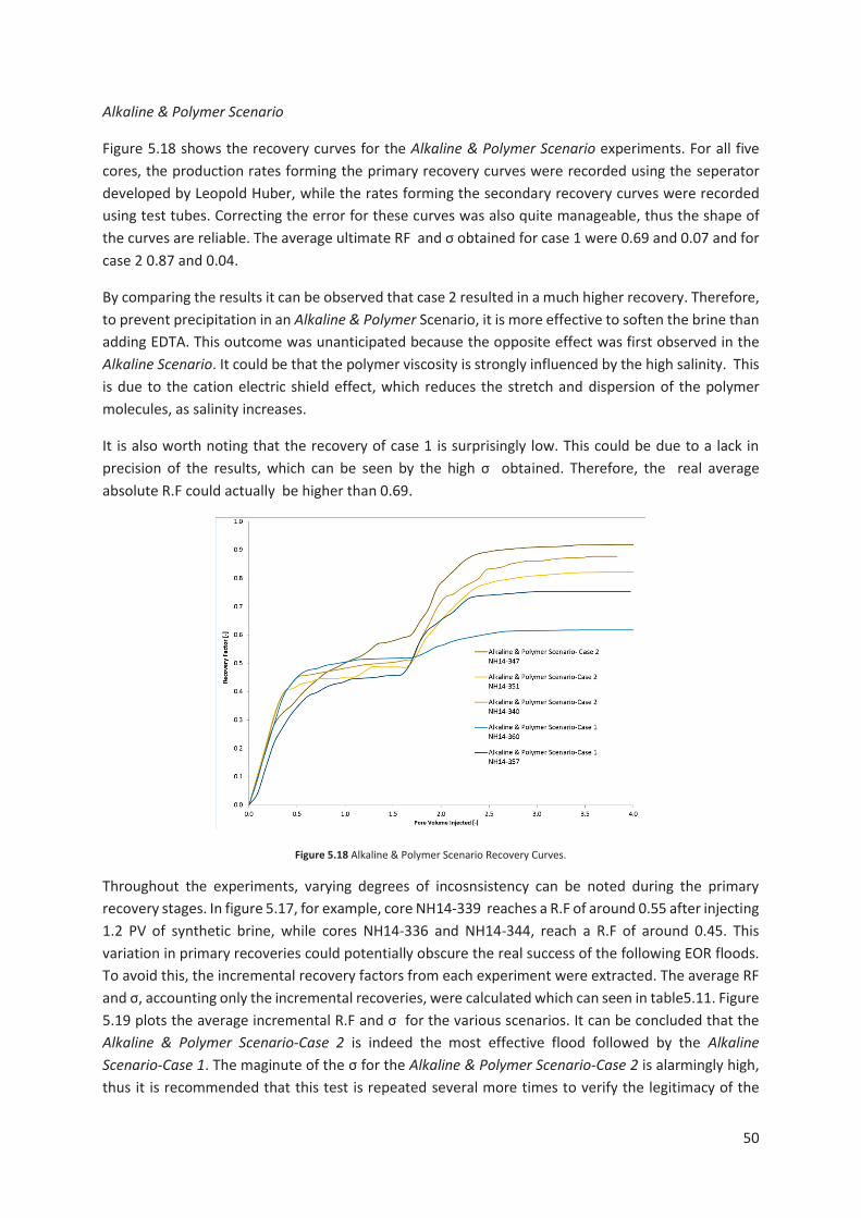
50

Alkaline & Polymer Scenario

Figure 5.18 shows the recovery curves for the Alkaline & Polymer Scenario experiments. For all five cores, the production rates forming the primary recovery curves were recorded using the seperator developed by Leopold Huber, while the rates forming the secondary recovery curves were recorded using test tubes. Correcting the error for these curves was also quite manageable, thus the shape of the curves are reliable. The average ultimate RF and σ obtained for case 1 were 0.69 and 0.07 and for case 2 0.87 and 0.04.

By comparing the results it can be observed that case 2 resulted in a much higher recovery. Therefore, to prevent precipitation in an Alkaline & Polymer Scenario, it is more effective to soften the brine than adding EDTA. This outcome was unanticipated because the opposite effect was first observed in the Alkaline Scenario. It could be that the polymer viscosity is strongly influenced by the high salinity. This is due to the cation electric shield effect, which reduces the stretch and dispersion of the polymer molecules, as salinity increases.

It is also worth noting that the recovery of case 1 is surprisingly low. This could be due to a lack in precision of the results, which can be seen by the high σ obtained. Therefore, the real average absolute R.F could actually be higher than 0.69.

Figure 5.18 Alkaline & Polymer Scenario Recovery Curves.

Throughout the experiments, varying degrees of incosnsistency can be noted during the primary recovery stages. In figure 5.17, for example, core NH14-339 reaches a R.F of around 0.55 after injecting 1.2 PV of synthetic brine, while cores NH14-336 and NH14-344, reach a R.F of around 0.45. This variation in primary recoveries could potentially obscure the real success of the following EOR floods. To avoid this, the incremental recovery factors from each experiment were extracted. The average RF and σ, accounting only the incremental recoveries, were calculated which can seen in table5.11. Figure 5.19 plots the average incremental R.F and σ for the various scenarios. It can be concluded that the Alkaline & Polymer Scenario-Case 2 is indeed the most effective flood followed by the Alkaline Scenario-Case 1. The maginute of the σ for the Alkaline & Polymer Scenario-Case 2 is alarmingly high, thus it is recommended that this test is repeated several more times to verify the legitimacy of the

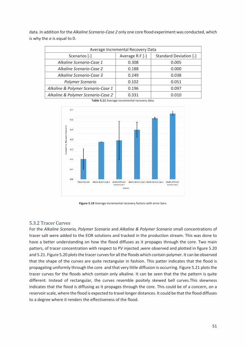
51

data. In addition for the Alkaline Scenario-Case 2 only one core flood experiment was conducted, which is why the σ is equal to 0.

Average Incremental Recovery Data Scenarios [-] Average R.F [-] Standard Deviation [-]

Alkaline Scenario-Case 1 0.308 0.005 Alkaline Scenario-Case 2 0.188 0.000 Alkaline Scenario-Case 3 0.249 0.038

Polymer Scenario 0.102 0.051 Alkaline & Polymer Scenario-Case 1 0.196 0.097 Alkaline & Polymer Scenario-Case 2 0.331 0.010

Table 5.11 Average incremental recovery data.

Figure 5.19 Average incremental recovery factors with error bars.

5.3.2 Tracer Curves For the Alkaline Scenario, Polymer Scenario and Alkaline & Polymer Scenario small concentrations of tracer salt were added to the EOR solutions and tracked in the production stream. This was done to have a better understanding on how the flood diffuses as it propages through the core. Two main patters, of tracer concentration with respect to PV injected ,were observed and plotted in figure 5.20 and 5.21. Figure 5.20 plots the tracer curves for all the floods which contain polymer. It can be observed that the shape of the curves are quite rectangular in fashion. This patter indicates that the flood is propagating uniformly through the core and that very little diffusion is occurring. Figure 5.21 plots the tracer curves for the floods which contain only alkaline. It can be seen that the the pattern is quite different. Instead of rectangular, the curves resemble positely skewed bell curves.This skewness indicates that the flood is diffusing as it propages through the core. This could be of a concern, on a reservoir scale, where the flood is expected to travel longer distances. It could be that the flood diffuses to a degree where it renders the effectiveness of the flood.

52

Figure 5.20 Tracer concentration curves for floods containing polymer.

Figure 5.21 Tracer concentration curves for floods containing only alkaline.

5.3.3 pH Curves For the Alkaline & Polymer Scenario the pH of the effluent were recorded. The pH with respect to PV injected for each flood is plotted in figure 5.22. The curves depict a similar pattern to the tracer curves in figure 5.20, which is to be expected. It can be noted that the pH peaks at a lower value for the Case-1 floods than the Case-2 floods. This could have occurred because the pH of the Case-1 experiments were measured 3 weeks after the experiments was conducted, unlike for Case-2, where the pH were measured the following day. As mentioned in the literature review, alkaline can be consumed over time as it reacts to hydrolyze the polymer. It could be that during this 3 week period, significant alkaline consumption took place to cause a reduction in pH. If correct, this could be concerning because a reduction in alkalinity over time means a degredation of the flood’s success.

53

Figure 5.22 pH concentration curves.

5.3.3 Polymer Concentration Curves In the literature review, it was mentioned that polymer adsorption can be reduced by adding an alkaline agent to the solution. Cummulative polymer recovery curves were derived to see if polymer adsorption was lower in the Alkaline & Polymer Scenario than the Polymer Scenario. Figure 5.23 plots the cumulative polymer RF with respect to PV injected. Table 5.12 shows the average total polymer recovery for each flooding scenario. The calculations deriving these values can be found in section C.3 in appendix C. By looking at the values in table 5.12, it can be noted that more polymer was recoverd in the Polymer Scenario than both the cases of Alkaline & Polymer Scenario. This is an odd observation. It could be that at the core-scale, it is difficult to accurately note a difference, and that this observation is simply coincidental.

Figure 5.23 Polymer cummulative recovery curves.

54

Polymer Recovery Data

Scenario Core

Number [-]

Total Polymer

R.F [-]

Average Total Polymer Recovery for each

Scenario [-]

Polymer Scenario 14-336 0.92 0.895 14-339 0.87

Alkaline & Polymer Scenario-Case 1

14-360 0.87 0.855 14-357 0.84 Alkaline & Polymer

Scenario-Case 2 14-347 0.91 0.885 14-351 0.86

Table 5.12 Polymer recovery data.

5.3.4 Concluding Remarks The core flooding experiments were conducted to have a better understanding on how alkaline, polymer, EDTA and brine softening affect the recovery. From the recovery curves it was found that the most effective flood is the Alkaline & Polymer Scenario-Case 2, with a measured average incremental RF of 0.331. In this case the flood consists of: the alkaline agent (1%wt Na2CO3), the polymer agent (800ppm FLOPAM 3630s) and the softened synthetic brine to prevent precipitation prior to injection. It was also found that alkaline is the element contributing the most to recovery. The average incremental R.F for the Alkaline Scenario is 0.25 ,while for the Polymer Scenario is only 0.10. Thirdly, it was found that precipitation occurring within the core does not have a negative impact on recovery. This was noted by comparing the recovery of the Alkaline Scenario-Case 1 to Alkaline Scenario-Case 2 where twice the required EDTA concentration was placed to reduce precipitation and resulted in a lower recovery. Also, for several scenarios, a high σ was measured indicating that the experiments should be repeated several more times to improve the reliability of the results.

From the tracer curves, two distint patterns were observed, revealing how the floods diffuse as they travel through the core. It was noted that diffusion is noticeably lower when polymer is present, thus the polymer is indeed effective at providing mobility control to the flood. From the alkaline curves, it was found that the pH follows the same pattern to the tracer curves. Lower pH values were recorded for samples which were recorded at a later time, indicating that the alkaline is being consumed over time. From the polymer curves, the average polymer recovery recorded was 88%. An improvement in recovery for the Alkaline & Polymer Scenario over the Polymer Scenario was not noted.

Chapter 6: Conclusion In this master thesis an emulsion and a core flooding study were conducted to see whether alkaline and polymer flooding could potentially improve the recovery of the 8TH and 16TH reservoirs of the Matzen field.

The purpose of the emulsion study was to understand how emulsification is influenced by the type of alkaline, alkaline concentration, solution salinity, divalent ions and solution/oil volume ratio. To do so, various alkaline solutions were mixed with crude coming from the 8TH reservoir. It was observed that the salinity has a strong influence on emulsification. It was found that no micro-emulsion would form at a salinities above 15,000 ppm. It was also found that Na2CO3 was much more tolerant of divalent ions than NaOH. However, mixing Na2CO3 with the synthetic brine, which contains Ca2+ ions, lead immediate precipitation of carbonate scale. For the future, it is recommended that the IFT is directly

55

measured for the various solutions. In this fashion it would be possible to calibrate the flood to obtain the lowest IFT possible.

The core flooding study was done to test various flood compositions. For the experiments the oil rate, water rate, tracer concentration, polymer concentration and pH were measured. It was found that the most effective flood composition was the Alkaline & Polymer Scenario-Case 3. This flood consisted of the alkaline agent (1%wt Na2CO3), the polymer agent (800ppm FLOPAM 3630s) and the softened synthetic brine to prevent precipitation prior to injection. The flood resulted in an incremental recovery factor of 0.331 after secondary recovery. It was also found that the alkaline agent is the main contributor to recovery and that carbonate precipitation, occurring within the core, does not negatively impact the recovery. From the pH measurements, it appeared that alkaline was being consumed by reacting with the polymer. From the polymer curves, the results showed no indication of a decrease in polymer adsorption when alkaline is present in the solution. For the future, it is recommended that these experiments are repeated several more times because, for several scenerios, large error bars were obtained.

56

Chapter 7: References Brouwer, D. R., J. D. Jansen, S. van der Starre, C. P. J. W. van Kruijsdijk, and C. W. J. Berentsen. 2001.

"Recovery Increase through Water Flooding with Smart Well Technology." In.: Society of Petroleum Engineers.

Cheng, K. H. 1986. "Chemical Consumption During Alkaline Flooding: A Comparative Evaluation." In.: Society of Petroleum Engineers.

deZabala, E.F., Vislocky, J.M., Rubin, E., Radke, C.J. , . 1982. 'A chemical theory for linear alkaline flooding', SPEJ, April: 245–58.

Dominguez, J. G., and G. P. Willhite. 1977. 'Retention and Flow Characteristics of Polymer Solutions in Porous Media'.

Ehrlich, Robert, and Robert J. Wygal, Jr. 1977. 'Interrelation of Crude Oil and Rock Properties With the Recovery of Oil by Caustic Waterflooding'.

Fan, Tianguang, and Jill S. Buckley. 2007. 'Acid Number Measurements Revisited'. Gruenwalder, Markus, Stefan Poellitzer, and Torsten Clemens. 2007. "Assisted and Manual History

Matching of a Reservoir with 120 Wells, 58 Years Production History and Multiple Well Re-Completions." In.: Society of Petroleum Engineers.

Hölzel M., Decker K., Zámolyi A., Strauss P., Wagreich M. 2010. ' Lower Miocene structural evolution of the central Vienna Basin (Austria) ', Marine and Petroleum Geology.: 666–81.

Jennings, H. Y., Jr., C. E. Johnson, Jr., and C. D. McAuliffe. 1974. 'A Caustic Waterflooding Process for Heavy Oils'.

Johnson, C. E., Jr. 1976. 'Status of Caustic and Emulsion Methods'. Kang, W.-L. 2001. 'Study of Chemical Interactions and Drive Mechanisms in Daqing ASP Flooding',

Petroleum Industry Press. Katsanis, E. P., P. H. Krumrine, and J. S. Falcone, Jr. 1983. "Chemistry of Precipitation and Scale

Formation in Geological Systems." In.: Society of Petroleum Engineers. Kienberger, Gerhard, and Reinhard Fuchs. 2006. "A Case History of the Matzen Field - 16thTorton: A

Story of Success! Where is the End?" In.: Society of Petroleum Engineers. Krumrine, P. H., and J. S. Falcone, Jr. 1987. "Beyond Alkaline Flooding: Design of Complete Chemical

Systems." In.: Society of Petroleum Engineers. Labrid, J. Bavière, M. 1991. The use of alkaline agents in enhanced oil recovery processes. . Lai, Hung. 2008. Defining Enhanced Oil Recovery. Laoroongroj, Ajana, Thomas Gumpenberger, and Torsten Clemens. 2014. "Polymer Flood

Incremental Oil Recovery and Efficiency in Layered Reservoirs Including Non-Newtonian and Viscoelastic Effects." In.: Society of Petroleum Engineers.

Laoroongroj, Ajana, Markus Lüftenegger, Rainer Kadnar, Christoph Puls, and Torsten Clemens. 2015. "Using Tracer Data to Determine Polymer Flooding Effects in a Heterogeneous Reservoir, 8 TH Reservoir, Matzen Field, Austria." In.: Society of Petroleum Engineers.

Martin, F. D., M. J. Hatch, J. S. Shepitka, and J. S. Ward. 1983. "Improved Water-Soluble Polymers for Enhanced Recovery of Oil." In.: Society of Petroleum Engineers.

McDougall, S. R., and K. S. Sorbie. 1993. "The Combined Effect of Capillary and Viscous Forces on Waterflood Displacement Efficiency in Finely Laminated Porous Media." In.: Society of Petroleum Engineers.

Mohnot, S. M., and J. H. Bae. 1989. 'A-Study of Mineral/Alkali Reactions-Part 2'. Moore, T. F., and R. L. Slobod. 1955. "Displacement of Oil by Water-Effect of Wettability, Rate, and

Viscosity on Recovery." In.: Society of Petroleum Engineers. Mungan, Necmettin. 1966. 'Certain Wettability Effects In Laboratory Waterfloods'. Pope, G. A., Ben Wang, and Kerming Tsaur. 1979. 'A Sensitivity Study of Micellar/Polymer Flooding'. Potts, D. E., and D. L. Kuehne. 1988. 'Strategy for Alkaline/Polymer Flood Design With Berea and

Reservoir-Rock Corefloods'. Sheng, D.-C., Yang, P.-H., Liu, Y.-L. 1993. 'Alkali-polymer interaction and alkali+polymer/crude

IFT', Oilfield Chemistry: 46–50.

57

———. 1994. 'Effect of alkali-polymer interaction on the solution properties. Petroleum Exploration and Development': 81–85.

Sheng, James J. 2011. 'Modern chemical enhanced oil recovery : theory and practice', Elsevier. Shuler, P.J., Kuehne, D.L., Lerner, R.M. 1989. 'Improving chemical flood efficiency with

micellar/alkaline/polymer process', JPT: 80–88. Shupe, Russell D. 1981. 'Chemical Stability of Polyacrylamide Polymers'. Subkow, P. 1942. "Process for the removal of bitumen from bituminous deposits." In. US. Szabo, Miklos T. 1979. 'An Evaluation of Water-Soluble Polymers For Secondary Oil Recovery - Parts 1

and 2'. Yang, P.-H., et al. 1992. ' Oil recovery mechanisms of alkaline/polymer flooding.'. Zhao, S., Zhang, L., Luo, L., Yu. 2002. 'Synergy between displacement agents and the active

components of crude oils. ', China Petrochemical Press., Fundamentals and Advances in Combined Chemical Flooding.

58

APPENDIX A: Data of Important Properties A.1 Figures

Figure A. 1 Viscosity and density as a function of temperature of stock tank oil coming from the 8TH reservoir.

A.2 Tables

Salts Molecular Weight [g/mol] Concentration [g/L]NaCl 58.44 23.93

NaAc*3H20 136.06 0.34CaCl2*2H20 147.01 1.15

Synthethic Brine Composition

Synthetic Brine Ionic Composition Ion [-] Concentration [g/L] Ion Concentration [ppm]

Na+ 9.471 9471 Cl- 15.071 15071

Ca2+ 0.313 313 Ac- 0.148 148

Brine Salinity [ppm] 25003 Table A. 1 Synthetic brine composition, mimicking the 8th reservoir of the Matzen field.

59

Core samples CCA Data

Core number [-] Bulk Volume [cc]

Pore Volume [cc]

Porosity [-] Permeability [mD]

14/334 51.538 11.328 0.220 2322.292 14/336 50.724 11.004 0.217 2339.523 14/337 51.594 11.452 0.222 2412.786 14/338 52.030 11.644 0.224 2376.560 14/339 49.881 10.559 0.212 2369.081 14/340 50.780 11.739 0.231 2731.573 14/344 51.138 11.238 0.220 2505.835 14/346 51.004 11.472 0.225 2556.968 14/347 50.780 11.223 0.221 2410.157 14/348 51.559 11.451 0.222 2425.758 14/350 50.990 11.324 0.222 2407.926 14/351 48.652 10.926 0.225 2445.423 14/357 50.696 10.847 0.214 2523.321 14/358 51.840 11.504 0.222 2519.150 14/360 50.969 11.644 0.228 2548.596

Table A. 2 CCA data for each core.

Experiment Data Required for Core Flood Saturation Calculation

Property Value Density brine Room Temp [g/cc] 1.01

Density brine Reservoir Temp [g/cc] 0.996 Density of Crude Oil [g/cc] 0.93

Density Live Oil @ 50 C [g/cc] 0.891 Viscosity Live Oil @ 50 C [cp] 20

Viscosity Crude Oil @ 50 C [cp] 40.6 Injection Rate Live Oil [mL/min] 0.5 Injection Rate Flood [mL/min] 1

Table A. 3 Experiment data required for Core Flood saturation calculations.

60

Core Flooding Experiment Summary

Core Number [-] Dry Weight [g]

Weight when Saturated with Brine [g]

Weight After Drainage Process

[g]

Weight after EOR Flood [g] Swir [-] Sw after

Flood [-] OOIP [cc] Oil Produced [cc]

Recovery Factor [-]

14/334 209.815 221.256 220.502 220.832 0.203 0.776 9.025 6.489 0.719 14/336 205.924 217.038 216.254 216.541 0.132 0.703 9.547 6.273 0.657 14/337 207.519 219.086 218.452 218.671 0.373 0.787 7.183 4.749 0.661 14/338 210.923 222.683 221.906 222.284 0.201 0.806 9.306 7.050 0.758 14/339 201.591 212.256 211.609 211.797 0.283 0.719 7.568 4.597 0.607 14/340 203.85 215.706 214.921 215.401 0.199 0.885 9.407 8.058 0.857 14/344 205.69 217.040 216.269 216.475 0.172 0.654 9.301 5.411 0.582 14/346 205.765 217.352 216.586 216.947 0.200 0.796 9.176 6.840 0.745 14/347 206.139 217.474 216.66 217.233 0.113 0.928 9.955 9.146 0.919 14/348 206.769 218.335 217.562 217.714 0.189 0.616 9.286 4.892 0.527 14/350 204.486 215.923 215.183 215.559 0.222 0.826 8.814 6.848 0.777 14/351 195.966 207.001 206.278 206.687 0.209 0.859 8.640 7.098 0.821 14/357 203.96 214.915 214.198 214.542 0.210 0.805 8.566 6.452 0.753 14/358 208.937 220.556 219.794 219.871 0.208 0.566 9.109 4.113 0.452 14/360 205.554 217.314 216.534 216.776 0.197 0.693 9.352 5.773 0.617

Table A. 4 Core flooding experiment sum

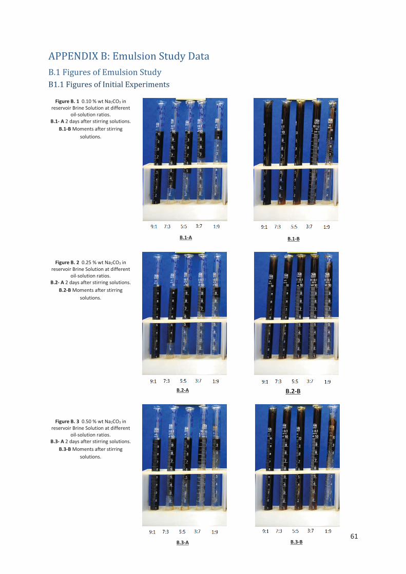
61

APPENDIX B: Emulsion Study Data B.1 Figures of Emulsion Study B1.1 Figures of Initial Experiments

B.1-A B.1-B

B.2-A B.2-B

B.3-A B.3-B

Figure B. 1 0.10 % wt Na2CO3 in reservoir Brine Solution at different

oil-solution ratios.

B.1- A 2 days after stirring solutions. B.1-B Moments after stirring

solutions.

Figure B. 3 0.50 % wt Na2CO3 in reservoir Brine Solution at different

oil-solution ratios. B.3- A 2 days after stirring solutions.

B.3-B Moments after stirring solutions.

Figure B. 2 0.25 % wt Na2CO3 in reservoir Brine Solution at different

oil-solution ratios.

B.2- A 2 days after stirring solutions. B.2-B Moments after stirring

solutions.

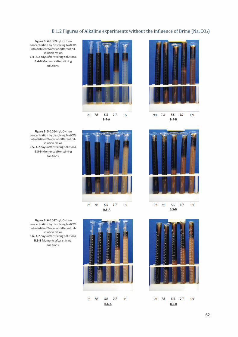
62

Figure B. 4 0.009 n/L OH- ion concentration by dissolving Na2CO3 into distilled Water at different oil-

solution ratios. B.4- A 2 days after stirring solutions.

B.4-B Moments after stirring solutions.

Figure B. 5 0.024 n/L OH- ion concentration by dissolving Na2CO3 into distilled Water at different oil-

solution ratios. B.5- A 2 days after stirring solutions.

B.5-B Moments after stirring solutions.

Figure B. 6 0.047 n/L OH- ion concentration by dissolving Na2CO3 into distilled Water at different oil-

solution ratios. B.6- A 2 days after stirring solutions.

B.6-B Moments after stirring. solutions.

B.1.2 Figures of Alkaline experiments without the influence of Brine (Na2CO3)

B.5-A

B.4-A

B.5-B

B.4-B

B.6-A B.6-B

63

Figure B. 7 0.094 n/L OH- ion concentration by dissolving Na2CO3 into distilled Water at different oil-

solution ratios. B.7 - A 2 days after stirring solutions.

B.7-B Moments after stirring solutions.

Figure B. 8 0.142 n/L OH- ion concentration by dissolving Na2CO3 into distilled Water at different oil-

solution ratios. B.8- A 2 days after stirring solutions.

B.8-B Moments after stirring solutions.

B.7-A B.7-B

B.8-A B.8-B

64

Figure B. 9 0.009 n/L OH- ion concentration by dissolving NaOH into distilled Water at different oil-

solution ratios. B.9- A 2 days after stirring solutions.

B.9-B Moments after stirring solutions.

Figure B. 10 0.024 n/L OH- ion concentration by dissolving NaOH into distilled Water at different oil-

solution ratio. B.10- A 2 days after stirring solutions.

B.10-B Moments after stirring solutions.

Figure B. 11 0.047 n/L OH- ion concentration by dissolving NaOH into distilled Water at different oil-

solution ratios. B.11- A 2 days after stirring solutions.

B.11-B Moments after stirring solutions.

B.1.3 Figures of Alkaline experiments without the influence of Brine (NaOH)

B.9-A B.9-B

B.10-A B.10-B

9-B

B.11-A B.11-B

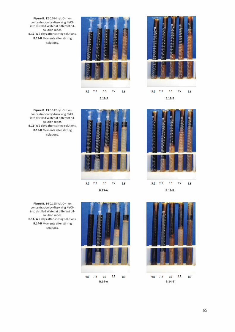
65

Figure B. 12 0.094 n/L OH- ion concentration by dissolving NaOH into distilled Water at different oil-

solution ratios. B.12- A 2 days after stirring solutions.

B.12-B Moments after stirring solutions.

Figure B. 13 0.142 n/L OH- ion concentration by dissolving NaOH into distilled Water at different oil-

solution ratios. B.13- A 2 days after stirring solutions.

B.13-B Moments after stirring solutions.

Figure B. 14 0.165 n/L OH- ion concentration by dissolving NaOH into distilled Water at different oil-

solution ratios. B.14- A 2 days after stirring solutions.

B.14-B Moments after stirring solutions.

B.12-A B.12-B

B.13-A B.13-B

B.14-A B.14-B

66

Figure B. 15 0.189 n/L OH- ion concentration by dissolving NaOH into distilled Water at different oil-

solution ratios. B.15- A 2 days after stirring solutions.

B.15-B Moments after stirring solutions.

Figure B. 16 0.236 n/L OH- ion concentration by dissolving NaOH into distilled Water at different oil-

solution ratios. B.16- A 2 days after stirring solutions.

B.16-B Moments after stirring solutions.

B.15-A B.15-B

B.16-A B.16-B

67

Figure B. 17 0.009 n/L Na2CO3 Concentration at various NaCl wt%

concentrations mixed at oil-solution ratios of 7:3.

B.17- A 2 days after stirring solutions. B.17-B Moments after stirring solutions.

Figure B. 18 0.024 n/L Na2CO3

Concentration at various NaCl wt% concentrations mixed at oil-solution ratios

of 7:3. B.18- A 2 days after stirring solutions.

B.18-B Moments after stirring solutions.

B.1.4 Figures of Salinity Experiments (Na2CO3)

0.0% 0.2% 0.4% 0.6% 0.8% 1.0% 1.2% 1.4% 1.6% 0.0% 0.2% 0.4% 0.6% 0.8% 1.0% 1.2% 1.4% 1.6%

0.0% 0.2% 0.4% 0.6% 0.8% 1.0% 1.2% 1.4% 1.6% 0.0% 0.2% 0.4% 0.6% 0.8% 1.0% 1.2% 1.4% 1.6%

B.18-A B.18-B

B.17-B B.17-A

68

Figure B. 19 .047 n/L Na2CO3 Concentration at various NaCl wt%

concentrations mixed at oil-solution ratios of 7:3.

B.19- A 2 days after stirring solutions. B.19-B Moments after stirring solutions.

Figure B. 20 0.071 n/L Na2CO3 Concentration at various NaCl wt%

concentrations mixed at oil-solution ratios of 7:3.

B.20- A 2 days after stirring solutions. B.20-B Moments after stirring solutions.

0.0% 0.2% 0.4% 0.6% 0.8% 1.0% 1.2% 1.4% 1.6% 0.0% 0.2% 0.4% 0.6% 0.8% 1.0% 1.2% 1.4% 1.6%

0.0% 0.2% 0.4% 0.6% 0.8% 1.0% 1.2% 1.4% 1.6% 0.0% 0.2% 0.4% 0.6% 0.8% 1.0% 1.2% 1.4% 1.6% B.20-A B.20-B

B.19-B B.19-A

69

Figure B. 21 0.094 n/L Na2CO3 Concentration at various NaCl wt%

concentrations mixed at oil-solution ratios of 7:3.

B.21- A 2 days after stirring solutions. B.21-B Moments after stirring solutions.

0.0% 0.2% 0.4% 0.6% 0.8% 1.0% 1.2% 1.4% 1.6% 0.0% 0.2% 0.4% 0.6% 0.8% 1.0% 1.2% 1.4% 1.6% B.21-B B.21-A

70

Figure B. 22 0.009 n/L NaOH Concentration at various NaCl wt%

concentrations mixed at oil-solution ratios of 7:3.

B.22- A 2 days after stirring solutions. B.22-B Moments after stirring solutions.

Figure B. 23 0.024 n/L NaOH Concentration at various NaCl wt%

concentrations mixed at oil-solution ratios of 7:3.

B.23- A 2 days after stirring solutions. B.23-B Moments after stirring solutions.

B.1.5 Figures of Salinity Experiments (NaOH)

0.0% 0.2% 0.4% 0.6% 0.8% 1.0% 1.2% 1.4% 1.6% 0.0% 0.2% 0.4% 0.6% 0.8% 1.0% 1.2% 1.4% 1.6%

0.0% 0.2% 0.4% 0.6% 0.8% 1.0% 1.2% 1.4% 1.6% 0.0% 0.2% 0.4% 0.6% 0.8% 1.0% 1.2% 1.4% 1.6% B.23-B B.23-A

B.22-A B.22-B

71

Figure B. 24 0.047 n/L NaOH Concentration at various NaCl wt%

concentrations mixed at oil-solution ratios of 7:3.

B.24- A 2 days after stirring solutions. B.24-B Moments after stirring solutions.

Figure B. 25 0.071 n/L NaOH Concentration at various NaCl wt%

concentrations mixed at oil-solution ratios of 7:3.

B.25- A 2 days after stirring solutions. B.25-B Moments after stirring solutions.

0.0% 0.2% 0.4% 0.6% 0.8% 1.0% 1.2% 1.4% 1.6% 0.0% 0.2% 0.4% 0.6% 0.8% 1.0% 1.2% 1.4% 1.6%

0.0% 0.2% 0.4% 0.6% 0.8% 1.0% 1.2% 1.4% 1.6% 0.0% 0.2% 0.4% 0.6% 0.8% 1.0% 1.2% 1.4% 1.6%

4.24-A B.24-B

B.25-B B.25-A

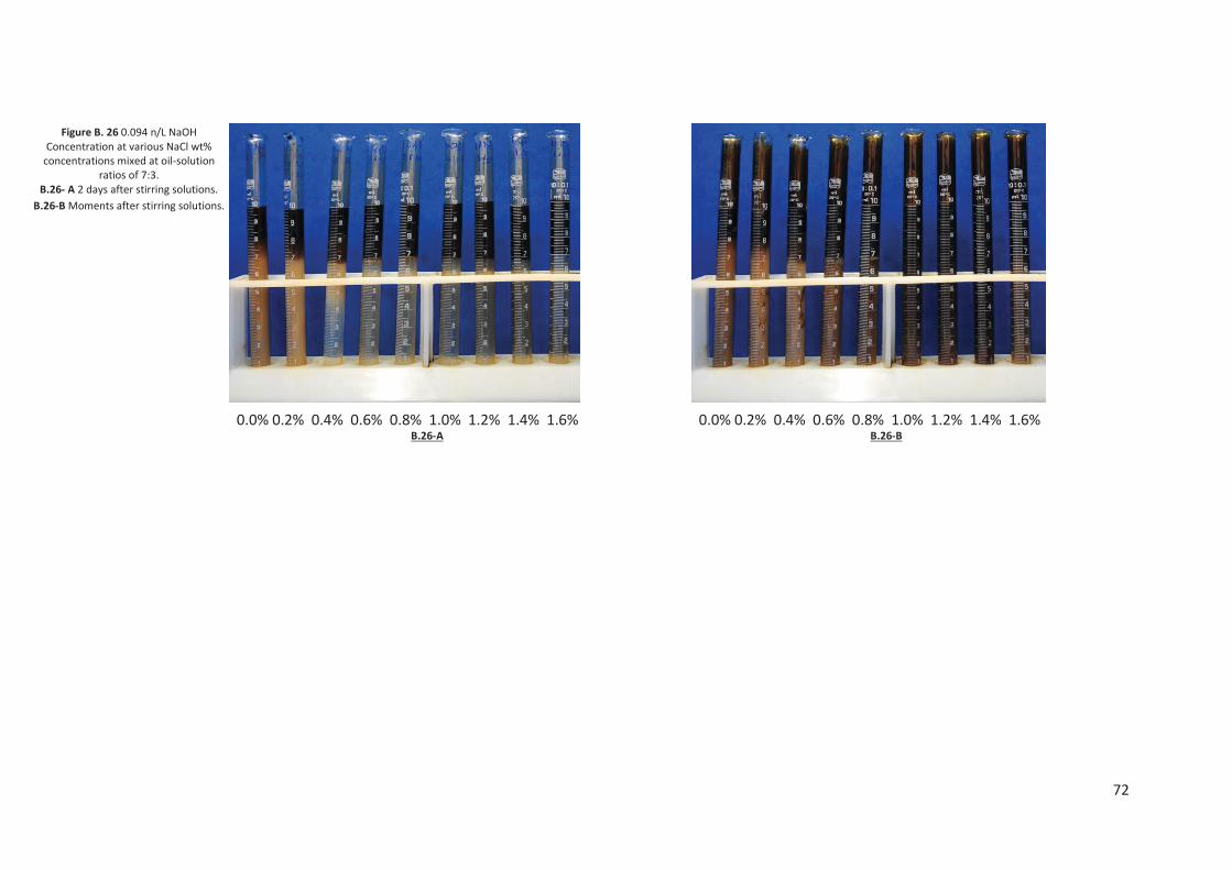
72

Figure B. 26 0.094 n/L NaOH Concentration at various NaCl wt%

concentrations mixed at oil-solution ratios of 7:3.

B.26- A 2 days after stirring solutions. B.26-B Moments after stirring solutions.

0.0% 0.2% 0.4% 0.6% 0.8% 1.0% 1.2% 1.4% 1.6% 0.0% 0.2% 0.4% 0.6% 0.8% 1.0% 1.2% 1.4% 1.6% B.26-A B.26-B