J. Fluid Mech. (2014), vol. 743, R3, doi:10.1017/jfm.2014.32

Alignment of vorticity and rods withLagrangian fluid stretching in turbulence

Rui Ni1,2, Nicholas T. Ouellette2 and Greg A. Voth1,†

1Department of Physics, Wesleyan University, Middletown, Connecticut 06459, USA2Department of Mechanical Engineering and Materials Science, Yale University,New Haven, CT 06520, USA

(Received 31 October 2013; revised 13 December 2013; accepted 12 January 2014)

Stretching in continuum mechanics is naturally described using the Cauchy–Greenstrain tensors. These tensors quantify the Lagrangian stretching experienced by amaterial element, and provide a powerful way to study processes in turbulent fluidflows that involve stretching such as vortex stretching and alignment of anisotropicparticles. Analysing data from a simulation of isotropic turbulence, we observepreferential alignment between rods and vorticity. We show that this alignmentarises because both of these quantities independently tend to align with the strongestLagrangian stretching direction, as defined by the maximum eigenvector of the leftCauchy–Green strain tensor. In particular, rods approach almost perfect alignmentwith the strongest stretching direction. The alignment of vorticity with stretching isweaker, but still much stronger than previously observed alignment of vorticity withthe eigenvectors of the Eulerian strain rate tensor. The alignment of strong vorticityis almost the same as that of rods that have experienced the same stretching.

Key words: particle/fluid flows, turbulent flows, vortex dynamics

1. Introduction

Stretching of a fluid element in a turbulent flow is a dynamic process that isnaturally expressed in the Lagrangian framework. For three-dimensional flows, thisprocess can be visualized by considering a sphere that is distorted into a tri-axialellipsoid as it is stretched by the flow. In continuum mechanics, the deformation ofan object is commonly described by the deformation gradient tensor F ij = (∂xi/∂Xj),where X is an initial position and x is a final position. After a sphere is deformed

† Email address for correspondence: gvoth@wesleyan.edu

c© Cambridge University Press 2014

743 R3-1

R. Ni, N. T. Ouellette and G. A. Voth

into an ellipsoid, the orientations of the three principal axes of the ellipsoid aregiven by the eigenvectors of the left Cauchy–Green strain tensor C(L)= FF T (Malvern1969).

In studies of turbulence, the most widely used properties of the Cauchy–Greenstrain tensor have been its eigenvalues, which specify the lengths of the principalaxes and therefore the shape of the ellipsoid (Girimaji & Pope 1990; Lüthi, Tsinober& Kinzelbach 2005; Guala et al. 2006). The eigenvalues are directly related to theLyapunov exponents (also known as the stretching rates) (Pierrehumbert & Yang 1993;Bec et al. 2006). One application that uses the eigenvalues has been identificationof Lagrangian coherent structures (Green, Rowley & Haller 2007; Peacock & Haller2013), which provide insights into mixing and transport.

In this paper, we show that the eigenvectors of the Cauchy–Green strain tensorprovide a Lagrangian basis in which the alignment of both passive vectors andvorticity in three-dimensional turbulent flow is remarkably simple. Passive vectorsalong with thin rods and material line segments become preferentially aligned with thelongest principal axis of the ellipsoid, and at long times approach perfect alignmentwith the eigenvector corresponding to maximum stretching. Vorticity is more complexsince it is an active vector that is both amplified by stretching and affected byviscosity. We find that the vortex stretching process also leads to strong alignmentwith the direction of maximum stretching, but that the degree of alignment saturatesafter 10 τη, where τη is the Kolmogorov time scale.

There is an extensive literature on the alignment of both passive vectors andvorticity in turbulence. In many applications, orientation dynamics reduce to thepassive vector problem. These include the orientation of thin rods (Parsa et al.2011; Pumir & Wilkinson 2011; Einarsson, Angilella & Mehlig 2013; Gustavsson,Einarsson & Mehlig 2013), material line segments (Dresselhaus & Tabor 1991; Lüthiet al. 2005) and magnetic field lines in a medium with high conductivity (Monin& Yaglom 1975). Batchelor (1952) provided theoretical predictions for materialline and surface stretching based on the assumption of persistent straining over ashort period of time. Subsequently, both simulations (Girimaji & Pope 1990) andexperiments (Lüthi et al. 2005; Guala et al. 2006) have studied the stretching ofmaterial lines by focusing on the alignment of a material line with the eigenvectorsof the Eulerian strain rate tensor (ei, i= 1, 2, 3). These studies used the eigenvaluesof the Cauchy–Green tensor to determine the deformation of a material volume;however, neither made connections between the orientation of a material line andthe eigenvectors of the Cauchy–Green strain tensor. There are two studies (Parsaet al. 2011; Wilkinson, Bezuglyy & Mehlig 2011) that used the eigenvectors of theCauchy–Green strain tensor to understand the orientation of rods in two-dimensionalflow. In three-dimensional turbulent flow, Pumir & Wilkinson (2011) and Wilkinson& Kennard (2012) focused on the relative orientation of rods with respect to theEulerian strain rate tensor as well as the vorticity vector. They found that the rodsalign more strongly with the vorticity and identified that the stretching term in theequations of motion for both vorticity and rods is responsible for the alignment. Aswe explain below, the effect of the stretching term is to align both passive vectorsand the vorticity vector with the largest Lagrangian stretching direction.

In turbulence, Taylor (1938) conjectured that the turbulent cascade mechanismrelies on the amplification of vortices by stretching, which subsequently leadsto breakup of large vortices into smaller ones. Most previous studies of vortexstretching have considered the alignment of vorticity ω with the eigenvectors ofthe Eulerian strain rate tensor (Ashurst et al. 1987; Huang 1996), which give the

743 R3-2

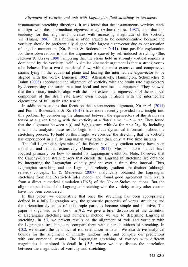
Alignment of vorticity and rods with Lagrangian fluid stretching in turbulence

instantaneous stretching directions. It was found that the instantaneous vorticity tendsto align with the intermediate eigenvector e2 (Ashurst et al. 1987), and that thetendency for this alignment increases with increasing magnitude of the vorticity|ω| (Huang 1996). This finding is often argued to be counterintuitive because thevorticity should be preferentially aligned with largest eigenvector due to conservationof angular momentum (Xu, Pumir & Bodenschatz 2011). One possible explanationfor these observations is that the alignment is caused by self-induced stretching (She,Jackson & Orszag 1990), implying that the strain field in strongly vortical regions isdominated by the vorticity itself. A similar kinematic argument is that a strong vortextube behaves like a two-dimensional flow, with the most extensive and compressivestrains lying in the equatorial plane and leaving the intermediate eigenvector to bealigned with the vortex (Jiménez 1992). Alternatively, Hamlington, Schumacher &Dahm (2008) approached the alignment of vorticity with the strain rate eigenvectorsby decomposing the strain rate into local and non-local components. They showedthat the vorticity tends to align with the most extensional eigenvector of the nonlocalcomponent of the strain rate tensor even though it aligns with the intermediateeigenvector of full strain rate tensor.

In addition to studies that focus on the instantaneous alignment, Xu et al. (2011)and Pumir, Bodenschatz & Xu (2013) have more recently provided new insight intothis problem by considering the alignment between the eigenvectors of the strain ratetensor at a given time t0 with the vorticity at a ‘later’ time t = t0 +1t. They foundthat the alignment between ω(t) and e1(t0) grows with 1t for 1t< 2τη. By includingtime in the analysis, these results begin to include dynamical information about thestretching process. To build on this insight, we consider the stretching that the vorticityhas experienced in a fully Lagrangian way rather than only at two time instants.

The full Lagrangian dynamics of the Eulerian velocity gradient tensor have beenmodelled and studied extensively (Meneveau 2011). Most of those studies havefocused primarily on how to model its Lagrangian evolution. Note, however, thatthe Cauchy–Green strain tensors that encode the Lagrangian stretching are obtainedby integrating the Lagrangian velocity gradient over a finite time interval. Thus,Lagrangian stretching and the Lagrangian velocity gradient are distinct (althoughrelated) concepts. Li & Meneveau (2007) analytically obtained the Lagrangianstretching from the Restricted-Euler model, and found good agreement with resultsfrom a direct numerical simulation (DNS) of the Navier–Stokes equations. But thealignment statistics of the Lagrangian stretching with the vorticity or any other vectorshave not been considered.

In this paper, we demonstrate that once the stretching has been appropriatelydefined in a fully Lagrangian way, the geometric properties of vortex stretching andthe orientation dynamics of anisotropic particles become simple and intuitive. Thepaper is organized as follows. In § 2, we give a brief discussion of the definitionof Lagrangian stretching and numerical method we use to determine Lagrangianstretching. In § 3, we present results on the alignment of rods and vorticity withthe Lagrangian stretching, and compare them with other definitions of stretching. In§ 3.2, we discuss the dynamics of rod orientation in detail. We also derive analyticalbounds for the alignment of initially random rods, and compare our predictionswith our numerical results. The Lagrangian stretching of vortices with differentmagnitudes is explored in detail in § 3.3, where we also discuss the correlationbetween the magnitudes of vorticity and stretching.

743 R3-3

R. Ni, N. T. Ouellette and G. A. Voth

2. Methods

In this paper, we study the Lagrangian stretching as defined by the Cauchy–Greenstrain tensor by analysing data from a DNS of homogeneous isotropic turbulence(Benzi et al. 2009).

The data were generated from a simulation with N3 = 5123 collocation points,corresponding to a Taylor-microscale Reynolds number of Rλ = 180. A total of7 × 104 Lagrangian trajectories were followed for O(1) large-eddy turnover times,and the velocity gradient tensor at the tracer positions was stored. The time stepto integrate the Navier–Stokes equations and track particles was O(10−2τη), anddata along the particle trajectories are recorded every 0.1 τη. The orientations ofinfinitesimal rod-shaped Lagrangian tracers with an aspect ratio of 20 were obtainedby integrating Jeffery’s equation (Jeffery 1922) along each trajectory (Parsa et al.2012). This choice of aspect ratio is arbitrary; we find, however, that the orientationdynamics for rods with aspect ratio larger than about 10 are insensitive to the aspectratio, as they behave essentially as material line segments.

For completeness, we briefly discuss here the Cauchy–Green strain tensors,their eigenvectors, and how we compute them. More details can be found incontinuum-mechanics textbooks (Malvern 1969; Chadwick 1999). Consider aninfinitesimal spherical fluid element at some time t0. After a time 1t, it will ingeneral have been stretched into an ellipsoid. The position of any point X inside thespherical element at t0 will be mapped to a position x inside the ellipsoid at t= t0+1t.We can define a deformation gradient tensor that characterizes the deformationexperienced by the fluid element as Fij = (∂xi/∂Xj). The evolution equation of Fis dFij(t)/dt = Aik(t)Fkj(t), where A is the instantaneous velocity gradient, with theinitial condition Fij(t0) = δij. We obtain F (t) from the DNS data by integrating over1t using a fourth-order Runge–Kutta scheme. The deformation gradient tensor, ormonodromy matrix (Wilkinson et al. 2011), provides a Lagrangian description ofthe fluid stretching (Parsa et al. 2011; Wilkinson et al. 2011). When F is appliedto inertial particles rather than fluid elements, it describes the compressibility of thevelocity field of the inertial particles in the Lagrangian framework (IJzermans et al.2009; Reeks & Meneguz 2011).

Any affine deformation can be expressed as pure stretching followed by a rotationor as a rotation followed by pure stretching. Thus, the deformation gradient tensorcan be decomposed as F =RU =VR, where R is an orthogonal rotation tensor and Uand V are, respectively, the right and left stretch tensors. The stretching, without anycontribution from rotation, can be obtained from the two symmetric inner products ofF with itself:

C(L) = FF T = VRRTV T = V 2, (2.1)C(R) = F TF = UTRTRU = U2. (2.2)

Here C(L) and C(R) are, respectively, the left and right Cauchy–Green strain tensors.These two tensors have the same eigenvalues Λi (i= 1, 2, 3), but different eigenvectorseLi (left) and eRi (right). The largest eigenvalue, Λ1 > 1, indicates extension, thesmallest eigenvalue, Λ3 < 1, indicates contraction, and the intermediate eigenvaluecan indicate either extension or contraction.

The physical meaning of the eigenvectors of the two Cauchy–Green strain tensorscan be shown in a few simple steps. Consider a material line segment that is ‘initially’aligned with largest right eigenvector, l(t0)= eR1. After some 1t, the material line will

743 R3-4

Alignment of vorticity and rods with Lagrangian fluid stretching in turbulence

R

R

R

2520151050 2520151050

0.20.2

0.2

0.4

0.4

(b)(a)

(c)0.4

0.6

0.8

1.0

FIGURE 1. The alignment of rods (p(t)) and vorticity (ω(t)) with respect to differentdefinitions of the stretching: (a) the eigenvectors of the left Cauchy–Green strain tensor eLi;(b) the eigenvectors of the right Cauchy–Green strain tensor eRi; and (c) the eigenvectorsof the strain rate tensor at the initial time ei(t0). For all three panels, i = 1, 2, 3 arethe indices for the eigenvectors corresponding to the largest, intermediate and smallesteigenvalues of the tensor of interest, and the horizontal dashed lines show R = 1/3,corresponding to the alignment between two randomly oriented vectors.

be deformed into l(t) = F eR1. Multiplying both sides of the equation with C(L), wehave

C(L)l(t)= C(L)[F eR1] = FF TF eR1 = FC(R)eR1 = FΛ1eR1 =Λ1l(t). (2.3)

Thus, the ‘final’ direction of the material line, l(t) = l(t)/|l(t)|, is the eigenvectorof the left Cauchy–Green strain tensor that corresponds to the maximum eigenvalue,namely eL1. The same proof applies for the other two pairs of eigenvectors (eR2,eL2 and eR3, eL3). Material lines that initially align with an eigenvector of the righttensor end up aligned with the counterpart eigenvector of the left tensor. Hereafter,to capture their physical meaning, eR1 and eL1 are also referred to as the initial andfinal largest Lagrangian stretching directions, respectively. Similarly, e1 at times t0and t are referred to as the initial and final largest Eulerian stretching directions.

3. Results

3.1. Average alignments of rods and vorticityFigure 1 shows the alignment of infinitesimal rods p(t) and the vorticity ω(t) withboth the Lagrangian and Eulerian stretching directions. The alignment is quantifiedusing the square of the cosine of the angles between two unit vectors. Both rods andvorticity align most strongly with the final largest Lagrangian stretching direction, eL1,especially if we use time intervals of at least 1t= 10 τη to calculate eL1.

In figure 1(a), the degree of alignment of rods with eL1 is higher than it is forthe vorticity because infinitesimal rods are material line segments that passively alignwith eL1. The evolution of vorticity, on the other hand, is more complicated. Fromits equation of motion, the vorticity evolves both due to stretching by the velocitygradient tensor and to the tearing or reconnection at small scales that can be induced

743 R3-5

R. Ni, N. T. Ouellette and G. A. Voth

by viscosity. The stretching of vorticity is the same as the stretching of a materialline segment, and will tend to align the vorticity in the same direction as eL1. Indeed,figure 1(a) shows that the alignment between ω(t) and eL1 is very strong, but thatthis alignment reaches a plateau at 0.6 after 10 τη. We interpret this plateau as aresult of the dynamic balance between stretching, which moves ω(t) toward eL1, andviscous effects, which move them apart. For the same reason, ω cannot be perfectlyperpendicular to eL3 and eL2, as also seen in figure 1(a). We remark that, since bothrods and vorticity independently show strong alignment with eL1 due to the stretchingprocess, they must also align with each other (Pumir & Wilkinson 2011).

At 1t = 0, figure 1 tells us that the instantaneous alignments between rods (p)and the eigenvectors of the Eulerian strain-rate tensor ei are 0.40, 0.44 and 0.16for i = (1, 2, 3). These values indicate that rods are slightly more aligned with e2than e1, consistent with some previous work (Pumir & Wilkinson 2011). However,other studies have reported different results. Experimentally, Lüthi et al. (2005) andGuala et al. (2006) found that material lines with random initial orientations alignpreferentially with e1 after ∼ 6 τη. Wan (2008) studied the alignment of material linesat six different Reynolds numbers, ranging from Rλ = 17 to 430. He found that atshort times (t < 10 τη), material lines were preferentially oriented along e1, a findingconsistent with the experimental results (Lüthi et al. 2005; Guala et al. 2006). But inthe long-time limit (t > 10 τη), the alignment of material lines was very sensitive tothe Reynolds number. At Rλ= 17 and 430, material lines aligned more with e1, whileat intermediate Reynolds numbers (Rλ = 50, 73, 120 and 240), material lines alignedbetter with e2. In all of these cases, however, the observed alignment of materiallines with any of the ei was much weaker than the alignment we observe with theLagrangian stretching direction.

As time evolves, the alignment between the vorticity, ω, and the eigenvectorsof the left Cauchy–Green tensor eLi changes from 0.32, 0.52 and 0.16 at 1t = 0for i = (1, 2, 3), eventually saturating at 0.61, 0.33 and 0.06 at 1t = 15 τη. Thisevolution indicates that if we define stretching in a Lagrangian way rather than anEulerian one, the vorticity aligns with the largest stretching direction rather thanthe intermediate eigenvector. Numerous studies have proposed explanations for thepuzzling alignment between vorticity and the intermediate eigenvector of the Eulerianstrain rate (Ashurst et al. 1987; Huang 1996; Hamlington et al. 2008; Xu et al.2011); in a fully Lagrangian description, however, the alignment is much simpler.The vorticity becomes preferentially aligned with the largest stretching direction dueto angular momentum conservation, just as one would intuitively expect.

The alignment trends between both rods and the vorticity and eR1 and e1(t0) are verysimilar to each other, as shown in figure 1(b,c). To explain this similarity, we recallfirst that eR1 gives the direction in which an initial spherical fluid element will be moststrongly stretched after 1t. Similarly, e1(t0) is the direction of strongest stretching atthe initial time t0 (Pumir et al. 2013). Thus, the alignment of ω(t) and p(t) with eithereR1 or e1(t0) arises from the same dynamical picture. In each case, alignment with theinitially strongest stretching direction builds up over a short but finite time. But as 1tgrows, the direction of strongest stretching at the initial time becomes more and moreuncorrelated with the final orientation of the rods or vorticity. Thus, all of the curvesin figure 1(b,c) approach 1/3 (the value expected for randomly oriented vectors) inthe long time limit.

3.2. Rods: slow approach to perfect alignmentFigure 1(a) shows that within 15 τη, rods become almost perfectly perpendicular toeL3 and so lie in the plane S12 containing eL1 and eL2. Subsequently, over a much

743 R3-6

Alignment of vorticity and rods with Lagrangian fluid stretching in turbulence

102100

0.5

0.6

0.7

0.8

0.9

1.0

1.1

101

FIGURE 2. The alignment of the orientation of rods p(t) with respect to the largestLagrangian stretching direction eL1(t) as a function of l1/l2. From bottom to top, thesolid lines represent different 1t, spaced linearly from 1 τη to 15 τη. The lower dotted lineand the upper dash-dotted line show the ideal cases where a spherical fluid element hasbeen stretched into an axisymmetric ellipsoid (l2= l3) and a flat two-dimensional ellipsoid(l3 = 0) respectively.

longer time scale, they become parallel to eL1 and perpendicular to eL2. To understandthis slow alignment, we can again visualize stretching as the process of deforming asphere into an ellipsoid with principal axes of length li =

√Λi (i = 1, 2, 3). Since

the flow is incompressible, l1l2l3 = 1 and the stretching can be specified using onlytwo independent parameters. Note that the finite-time Lyapunov exponents are γi =ln(li)/1t (i= 1, 2, 3) (Bec et al. 2006).

In figure 2, the alignment between p(t) and eL1(t) is plotted as a function of l1/l2

for different 1t, ranging from 1 τη to 15 τη. For all 1t, the alignment increasesmonotonically with l1/l2, suggesting that the geometrical aspect ratio l1/l2 controlsthe orientation for the rods in the plane S12. The extension of each solid line givesus an idea of the width of the l1/l2 distribution. Both the mean value and the rangeof the ratio l1/l2 increase with increasing 1t. At 1t = 15 τη, l1/l2 varies over twoorders of magnitude, from 2 to more than 200. The alignment for large l1/l2 ∼ 100is almost perfect; but there are still a non-negligible number of samples with smalll1/l2 < 10 so that the overall alignment with eL1(t) is imperfect.

When visualizing stretching in 3D turbulence, it is useful to consider two limitingcases: deformation into pancake shapes (l1≈ l2� l3) and into cigar shapes (l1� l2≈ l3)(Girimaji & Pope 1990). For pancakes, the extreme case is a two-dimensional ellipsoidwith l3 approaching zero. In this case, rods will have lost all orientational freedomin the eL3 direction, which makes it more likely that they will be aligned with eL1(t).Thus, the thin pancake limit should be the upper bound for all curves for a given valueof l1/l2. To calculate the expected alignment in this case, we used a model proposedfor two-dimensional flow (Parsa et al. 2011); the results are shown with the dash-dotted line in figure 2. For cigars, which are axisymmetric ellipsoids with l2= l3, rods

743 R3-7

R. Ni, N. T. Ouellette and G. A. Voth

10−1 100 1010.1

0.2

0.3

0.4

0.5

0.6

0.7

0.8

0.9

1.0

FIGURE 3. The alignment of ω(t) with eL1 conditioned on the magnitude of vorticity|ω(t)| for different 1t, spaced linearly from 0 τη (bottom dash-dotted line) to 15 τη (topsolid line) with time step 1 τη. Note that the eL1 at 1t= 0 is equal to e1(t).

have the most freedom to align in the eL3 direction of all shapes with a given value ofl1/l2. Their alignment with eL1, therefore, will be the smallest as compared with othershapes. Here, we provide a simple analytic model to calculate this effect. Consider aradial material line in a unit sphere in the coordinate system {eLi}, whose projectionsonto the three directions are (x, y, z). If the initial orientation of the material line isuniformly distributed on the unit sphere, then the probability density function (PDF)of x is P(x)= 1/2 for x ∈ [−1, 1]. After 1t, the unit sphere will be stretched into anellipsoid with principal axes li. The material line will be mapped to the correspondingorientation in the ellipsoid, pointing along (l1x, l2y, l3z). Given the two extra conditionsl1l2l3 = 1 (incompressible flow) and l2 = l3 (an axisymmetric ellipsoid), we have

〈[p(t) · eL1]2〉 =∫ 1

−1

l21x2

l21x2 + l2

2y2 + l23z2

P(x) dx= 12

∫ 1

−1

s2

s2 + (1/x2 − 1)dx, (3.1)

where s= l1/l2 is the aspect ratio of the ellipsoid. The dotted line in figure 2 showsthe integration result in equation (3.1). If the rods were initially randomly oriented,this would be the lower bound for their alignment. In the simulation, however, weevolve rods with the turbulence until they reach a steady state before measuring theirorientational statistics, in order to obtain results that are closer to the experimentallymeasurable case of advected rods (Parsa et al. 2012). This steady state has a non-random initial orientation, which leads to alignments that are sometimes lower thanthe axisymmetric limit shown. Note that there are fewer points below the dotted lineas 1t increases, since the initial conditions become less and less relevant for larger1t.

3.3. Vortex stretching: effects of vorticity and stretching magnitudesPart of the reason for the imperfect alignment of vorticity with Lagrangian stretchingin figure 1 is that the result is averaged over all vorticity magnitudes. In figure 3, we

743 R3-8

Alignment of vorticity and rods with Lagrangian fluid stretching in turbulence

0 1–1

–1.0

–0.5

0.5

1.0

1.5

0

–1.0

–0.5

0.5

1.0

1.5

–1–6 –4 –2 00(a)

1 2

0

–2–3 0 1–1–2–3

log(p) (b) log(Q)

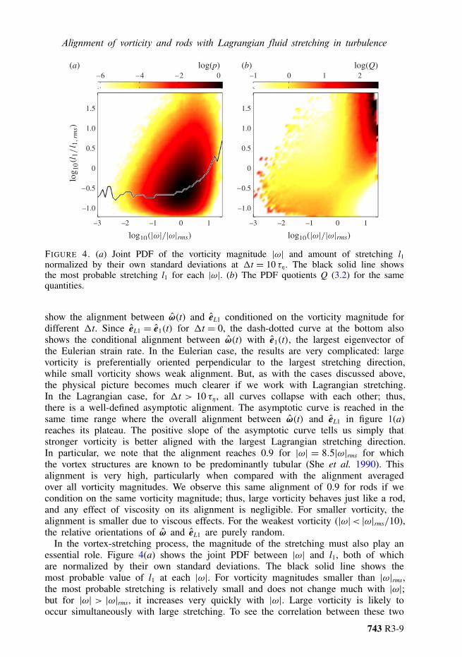
FIGURE 4. (a) Joint PDF of the vorticity magnitude |ω| and amount of stretching l1normalized by their own standard deviations at 1t = 10 τη. The black solid line showsthe most probable stretching l1 for each |ω|. (b) The PDF quotients Q (3.2) for the samequantities.

show the alignment between ω(t) and eL1 conditioned on the vorticity magnitude fordifferent 1t. Since eL1 = e1(t) for 1t = 0, the dash-dotted curve at the bottom alsoshows the conditional alignment between ω(t) with e1(t), the largest eigenvector ofthe Eulerian strain rate. In the Eulerian case, the results are very complicated: largevorticity is preferentially oriented perpendicular to the largest stretching direction,while small vorticity shows weak alignment. But, as with the cases discussed above,the physical picture becomes much clearer if we work with Lagrangian stretching.In the Lagrangian case, for 1t > 10 τη, all curves collapse with each other; thus,there is a well-defined asymptotic alignment. The asymptotic curve is reached in thesame time range where the overall alignment between ω(t) and eL1 in figure 1(a)reaches its plateau. The positive slope of the asymptotic curve tells us simply thatstronger vorticity is better aligned with the largest Lagrangian stretching direction.In particular, we note that the alignment reaches 0.9 for |ω| = 8.5|ω|rms for whichthe vortex structures are known to be predominantly tubular (She et al. 1990). Thisalignment is very high, particularly when compared with the alignment averagedover all vorticity magnitudes. We observe this same alignment of 0.9 for rods if wecondition on the same vorticity magnitude; thus, large vorticity behaves just like a rod,and any effect of viscosity on its alignment is negligible. For smaller vorticity, thealignment is smaller due to viscous effects. For the weakest vorticity (|ω|< |ω|rms/10),the relative orientations of ω and eL1 are purely random.

In the vortex-stretching process, the magnitude of the stretching must also play anessential role. Figure 4(a) shows the joint PDF between |ω| and l1, both of whichare normalized by their own standard deviations. The black solid line shows themost probable value of l1 at each |ω|. For vorticity magnitudes smaller than |ω|rms,the most probable stretching is relatively small and does not change much with |ω|;but for |ω| > |ω|rms, it increases very quickly with |ω|. Large vorticity is likely tooccur simultaneously with large stretching. To see the correlation between these two

743 R3-9

R. Ni, N. T. Ouellette and G. A. Voth

variables in another way, we also plot in figure 4(b) the PDF quotients Q, defined as(Xu, Ouellette & Bodenschatz 2007)

Q(|ω|, l1)≡ P(|ω|, l1)

P(|ω|)P(l1). (3.2)

Here Q gives a measure of the correlation between these two variables, since Q =1 for uncorrelated variables; Q > 1 means positive correlation, while Q < 1 meansanticorrelation. The very high correlation between the two quantities in the top rightcorner suggests that, indeed, intense vortices have undergone strong stretching. Forweak vortices, there are only very small positive (negative) correlations with small(large) amounts of stretching because, for those vortices, viscous damping is strongrelative to stretching.

4. Summary

We used the results of a DNS of turbulence to study Lagrangian stretching byusing the Cauchy–Green strain tensors. We have shown that the eigenvectors ofthe left and right Cauchy–Green tensors give a natural basis for studying phenomenainvolving stretching. In this paper, we have demonstrated this idea using the alignmentstatistics of two vectors: rod-like particles (essentially material line segments) and thevorticity vector. Both rods and the vorticity vector tend to be aligned with the largestLagrangian stretching direction eL1, and the degree of alignment is stronger than it iswith stretching directions defined from Eulerian quantities.

Rods become perfectly aligned with eL1 in the long time limit. They rapidly becomeoriented in the plane S12 formed by eL1 and eL2. However, it takes much longer forthem to become perfectly aligned with eL1 because a fraction of the rods experiencenearly equal stretching in the eL2 direction.

The stretching of vorticity, as an active vector, is usually studied in the Eulerianframe by using the alignment of vorticity with the eigenvectors of the instantaneousstrain-rate tensor. Many studies have observed the puzzling result that vorticitytends to align most strongly with the intermediate eigenvector of the Eulerian strainrate. But after defining stretching in a Lagrangian basis, we find that the vorticitytends to align with the largest Lagrangian stretching direction, just as one wouldintuitively expect. In addition, the alignment of strong vorticity is almost exactlythe same as for rods, and large vorticities are correlated with the strong stretchingthey have experienced. Analysis of Lagrangian stretching provides a powerful toolfor understanding alignment of material lines and vorticity in turbulence. This toolhas the potential to illuminate many other problems including turbulent mixing, thedynamics of anisotropic particles with other shapes than thin rods, and the structureof the events responsible for internal intermittency.

Acknowledgements

We thank Federico Toschi and Enrico Calzavarini for providing us with the DNSdata. We acknowledge support from US NSF grants DMR-1206399 to Yale Universityand DMR-1208990 to Wesleyan University, and COST Actions MP0806 and FP1005.

References

ASHURST, WM. T., KERSTEIN, A. R., KERR, R. M. & GIBSON, C. H. 1987 Alignment of vorticityand scalar gradient with strain rate in simulated Navier–Stokes turbulence. Phys. Fluids 30,2343–2353.

743 R3-10

Alignment of vorticity and rods with Lagrangian fluid stretching in turbulence

BATCHELOR, G. K. 1952 The effect of homogeneous turbulence on material lines and surfaces. Proc.R. Soc. Lond. A 213, 349–366.

BEC, J., BIFERALE, L., BOFFETTA, G., CENCINI, M., MUSACCHIO, S. & TOSCHI, F. 2006 Lyapunovexponents of heavy particles in turbulence. Phys. Fluids 18, 091702.

BENZI, R., BIFERALE, L., CALZAVARINI, E., LOHSE, D. & TOSCHI, F. 2009 Velocity-gradientstatistics along particle trajectories in turbulent flows: The refined similarity hypothesis in theLagrangian frame. Phys. Rev. E 80, 066318.

CHADWICK, P. 1999 Continuum Mechanics: Concise Theory and Problems. Dover Publications.DRESSELHAUS, E. & TABOR, M. 1991 The kinematics of stretching and alignment of material

elements in general flow fields. J. Fluid Mech. 236, 415–444.EINARSSON, J., ANGILELLA, J. R. & MEHLIG, B. 2013 Orientational dynamics of weakly inertial

axisymmetric particles in steady viscous flows. Preprint ArXiv:1307.2821.GIRIMAJI, S. S. & POPE, S. B. 1990 Material-element deformation in isotropic turbulence. J. Fluid

Mech. 220, 427–458.GREEN, M. A., ROWLEY, C. W. & HALLER, G. 2007 Detection of Lagrangian coherent structures

in three-dimensional turbulence. J. Fluid Mech. 572, 111–120.GUALA, M., LIBERZON, A., LÜTHI, B., KINZELBACH, W. & TSINOBAR, A. 2006 Stretching and

tilting of material lines in turbulence: The effect of strain and voriticity. Phys. Rev. E 73,036303.

GUSTAVSSON, K., EINARSSON, J. & MEHLIG, B. 2014 Tumbling of small axisymmetric particles inrandom and turbulent flows. Phys. Rev. Lett. 112, 014501.

HAMLINGTON, P. E., SCHUMACHER, J. & DAHM, W. J. A. 2008 Direct assessment of vorticityalignment with local and nonlocal strain rates in turbulent flows. Phys. Fluids 20, 111703.

HUANG, M.-J. 1996 Correlations of vorticity and material line elements with strain in decayingturbulence. Phys. Fluids 8, 2203–2214.

IJZERMANS, R. H. A., REEKS, M. W., MENEGUZ, E., PICCIOTTO, M. & SOLDATI, A. 2009Measuring segregation of inertial particles in turbulence by a full Lagrangian approach. Phys.Rev. E 80, 015302(R).

JEFFERY, G. B. 1922 The motion of ellipsoidal particles immersed in a viscous fluid. Proc. R. Soc.Lond. A 102, 161–179.

JIMÉNEZ, J. 1992 Kinematic alignment effects in turbulent flows. Phys. Fluids 4, 652–654.LI, Y. & MENEVEAU, C. 2007 Material deformation in a restricted euler model for turbulent flows:

analytic solution and numerical tests. Phys. Fluids 19, 015104.LÜTHI, B., TSINOBER, A & KINZELBACH, W. 2005 Lagrangian measurement of vorticity dynamics

in turbulent flow. J. Fluid Mech. 528, 87–118.MALVERN, L. E. 1969 Introduction to the Mechanics of a Continuous Medium. Prentice-Hall.MENEVEAU, C. 2011 Lagrangian Dynamics and Models of the Velocity Gradient Tensor in Turbulent

Flows. Annu. Rev. Fluid Mech. 43, 219–245.MONIN, A. S. & YAGLOM, A. M. 1975 Statistical Fluid Mechanics. MIT Press.PARSA, S., CALZAVARINI, E., TOSCHI, F. & VOTH, G. A. 2012 Rotation rate of rods in turbulent

fluid flow. Phys. Rev. Lett. 109 (13), 134501.PARSA, S., GUASTO, J. S., KISHORE, M., OUELLETTE, N. T., GOLLUB, J. P. & VOTH, G. A. 2011

Rotation and alignment of rods in two-dimensional chaotic flow. Phys. Fluids 23, 043302.PEACOCK, T. & HALLER, T. 2013 Lagrangian coherent structures: The hidden skeleton of fluid flows.

Phys. Today 66, 41–48.PIERREHUMBERT, R. T. & YANG, H. 1993 Global chaotic mixing on isentropic surfaces. J. Atmos.

Sci. 50, 2480.PUMIR, A., BODENSCHATZ, E. & XU, H. 2013 Tetrahedron deformation and alignment of perceived

vorticity and strain in a turbulent flow. Phys. Fluids 25, 035101.PUMIR, A. & WILKINSON, M. 2011 Orientation statistics of small particles in turbulence. New J.

Phys. 13, 093030.REEKS, M. W. & MENEGUZ, E. 2011 Statistical properties of particle segregation in homogeneous

isotropic turbulence. J. Fluid Mech. 686, 338–351.

743 R3-11

R. Ni, N. T. Ouellette and G. A. Voth

SHE, Z.-S., JACKSON, E. & ORSZAG, S. A. 1990 Intermittent vortex structures in homogeneousisotropic turbulence. Nature 344, 226–228.

TAYLOR, G. I. 1938 Production and dissipation of vorticity in a turbulent fluid. Proc. R. Soc. Lond.A 164, 15–23.

WAN, M. 2008 On the lagrangian study of the turbulent energy and circulation cascades. PhD thesis.WILKINSON, M., BEZUGLYY, V. & MEHLIG, B. 2011 Emergent order in rheoscopic swirls. J. Fluid

Mech. 667, 158–187.WILKINSON, M. & KENNARD, H. R. 2012 A model for alignment between microscopic rods and

vorticity. J. Phys. A: Math. Theor. 45, 455502.XU, H., OUELLETTE, N. T. & BODENSCHATZ, E. 2007 Curvature of Lagrangian Trajectories in

Turbulence. Phys. Rev. Lett. 98, 050201.XU, H., PUMIR, A. & BODENSCHATZ, E. 2011 The pirouette effect in turbulent flows. Nature Phys.

7, 709–712.

743 R3-12