ALGORITMI DI OTTIMIZZAZIONE PER LA CALIBRAZIONE DI … · Scientific Section Acutis M.e...

Scientific Section Acutis M.e Confalonieri R. Italian Journal of Agrometeorology 26 - 34 (3) 2006

26

OPTIMIZATION ALGORITHMS FOR CALIBRATING CROPPING SYSTEMS SIMULATION MODELS. A CASE STUDY WITH SIMPLEX-DERIVED METHODS

INTEGRATED IN THE WARM SIMULATION ENVIRONMENT

ALGORITMI DI OTTIMIZZAZIONE PER LA CALIBRAZIONE DI MODELLI DI SIMULAZIONE DI SISTEMI COLTURALI. UN CASO DI STUDIO CON APPROCCI DERIVATI DAL SIMPLESSO

INTEGRATI NELL’AMBIENTE DI SIMULAZIONE DI WARM

Marco Acutis1*, Roberto Confalonieri2

1 Department of Crop Science, University of Milano, Via Celoria 2, 20133 Milano, Italy

2 Institute for the Protection and Security of the Citizen, Joint Research Centre of the European Commission, AGRIFISH Unit, MARS-STAT Sector, TP 268 - 21020 Ispra (VA), Italy

* Corresponding Author, Tel. +39-02-50316581, E-mail: [email protected], Fax: +39-02-50316575 Received 22/10/2006 – Accepted 6/12/2006

Abstract Calibration is the process of adjusting parameters values to obtain a good fit between model outputs and observations. The objective is to later apply the model to conditions similar to those characterizing the data used for the calibration. Even if calibration is a standard in model application, it is a high risk procedure. The purpose of calibration is to determine the val-ues of unknown variables or parameters on the basis of their effects; the underlying risk of calibration is to degrading a mechanistic model to a totally empirical model very similar to a regression model, but without the statistical support to the conclusion drawing from the latter type of model. A reliable calibration process includes four steps. Step 1 is to define a criterion to evaluate the performance of a model in terms of an objective function; step 2 is to select the variables (or pa-rameters) that will be calibrated; step 3 is to select an appropriate algorithm for minimisation (or maximisation) of the ob-jective function; step 4 is the test of calibration results against new data sets. This paper focuses on step 3, and in particular on discussing, testing, and comparing two optimization algorithms derived from the simplex method: a bounded version of the Downhill Simplex (BS) and a modified version of the Evolutionary Shuffled Simplex (ESS). The two algorithms, se-lected because they do not use derivatives (crop models are strongly not-linear), were tested using two standard benchmark functions for optimization methods: the Rosenbrock and the Rastrigin functions. Results show that, even if BS requires few model evaluations, in some cases it is not able to find a global minimum in a multidimensional complex hyperspace. In this case, a more performing algorithm (such as ESS) should be used. The two algorithms have been introduced in the WARM simulation environment, allowing WARM to run automatic cali-brations using both methods. Some results are presented. Keywords: Automatic calibration, Rastrigin, Rosenbrock, Downhill simplex, Evolutionary Shuffled Simplex. Riassunto La calibrazione è il processo attraverso il quale i valori di parametri vengono modificati al fine di ottenere un buon accor-do tra risultati di un modello e osservazioni. L’obiettivo è di applicare in seguito il modello a condizioni simili a quelle per le quali è stato calibrato. Anche se la calibrazione è una pratica normale nella modellistica di simulazione, è una procedu-ra altamente rischiosa. Il suo scopo, infatti, è di determinare il valore di grandezze incognite sulla base dei loro effetti; il rischio è di degradare un modello meccanicistico ad un modello totalmente empirico, ma senza il supporto statistico che caratterizza i modelli empirici. Una calibrazione affidabile include quattro fasi. La prima consiste nel definire un criterio per valutare le prestazioni di un modello, in altre parole identificare un’adeguata funzione obiettivo. La seconda prevede la selezione dei parametri da calibrare. La terza fase consiste nell’individuazione di un algoritmo di ottimizzazione appro-priato per la minimizzazione (o la massimizzazione) della funzione obiettivo. La quarta fase è la verifica dei risultati della calibrazione utilizzando nuovi dati sperimentali Questo articolo è focalizzato sulla terza fase, in particolare sulla discus-sione, verifica e confronto di due algoritmi di ottimizzazione derivati dal metodo del simplesso: una versione del Downhill Simplex con variazione delimitata dei parametri (BS) ed una versione modificata dell’Evolutionary Shuffled Simplex (ESS). I due algoritmi, selezionati in quanto non fanno uso di derivate (i modelli biofisici sono sistemi fortemente non lineari), so-no stati esaminati utilizzando due funzioni particolarmente adatte per valutare metodi di ottimizzazione: la funzione di Ro-senbrock e quella di Rastrigin. I risultati mostrano che, nonostante BS richieda poche iterazioni, in alcuni casi non è in grado di trovare un minimo globale in un iperspazio multidimensionale complesso; in questi casi, è necessario utilizzare algoritmi più potenti, come ad esempio ESS. I due algoritmi sono stati inseriti nell’ambiente di simulazione di WARM, rendendo il modello in grado di effettuare cali-brazioni automatiche utilizzando entrambi i metodi. Si forniscono alcuni risultati preliminari. Parole chiave: Calibrazione automatica, Rastrigin, Rosenbrock, Downhill simplex, Evolutionary Shuffled Simplex.


27

Introduction Calibration is the process which consists in adapting a model to one or more sets of measured data to succes-sively allow its application to similar conditions (Beck, 1987). Even if calibration is a standard in model applica-tion, it is a high risk procedure. The purpose of calibra-tion is to determine the values of unknown variables on the basis of their effects. This leads to the risk of reduc-ing a biophysical model to a black box. In fact, when a variable is used for calibration, it is possible to include in its value errors coming from other sectors of the model-ling process (e.g. errors in the estimation of other vari-ables, errors in conceptual representation of the system, effect of correlation with other variables).This reduces the procedure of calibration to a fitting procedure, de-grading a mechanistic model to a totally empirical one, very similar to a regression model but without its statisti-cal support. This risk, present also when calibration is carried out on only one variable, increases exponentially with the number of variables under calibration. In spite of this, it is absolutely unusual that a biophysical model performs adequately without calibration, so there is a clear need to define rigorous, low-risk criteria allowing to perform calibrations and avoiding the typical problems which arise from an extensive use of this procedure. The purpose of a calibrations is to improve the perform-ance of a model against a set of measured data, thus the first element needed for calibration is to define criteria to evaluate the performance of a model. The literature about the model evaluation is wide and dozens of performance indices have been proposed (e.g. Loague and Green 1991; Martorana and Bellocchi, 1999; Tedeschi, 2005). Moreover, model evaluations typically cannot be done using only one of these indices (e.g. Smith et al., 1997). The difficulty to evaluate simultaneously different indi-ces is usually handled using some aggregation criteria ranging from simple weighted sum to the more recent proposals of fuzzy logic application (Bellocchi et al, 2002). The problem of the multiplicity of indices is raised by the existence of several output variables of in-terest, which are characteristic of a biophysical model, e.g.: biomass, yield, leaf area index, drainage and leach-ing, evolution of organic matter in the soil. All of these variables are frequently simulated by cropping system models, and it is not reasonable to have excellent agree-ment between observed and simulated values only in one of these tightly correlated outputs without accounting for the others. In this case, in fact, no conclusions about the real ability of the model in “understanding” the simu-lated system should be derived. Another common mis-take in calibrations is to calibrate parameters “far” from the output: often the calibration is carried out on outputs that are not directly determined by the variable under calibration because of several interferences due to other processes. In this case, the calibrated variable tends to include errors in the simulation of the other processes involved: the result is a loss of the biophysical meaning of the calibrated variable. Also in this case, usually, the calibration leads to instability of the model, when applied on new datasets. The way to overcome this problem is to calibrate single, specific sub-models. This is not always

possible because of the unavailability of data for process-specific calibrations and of the computational structure of the model that usually does not allow process-specific inputs and outputs. Synthesizing the previous considerations, an effective calibration is possible only with modular, component-based models (Donatelli et al., 2004), which allow insu-lating the various processes involved in the full system model and, therefore, calibrating and testing each single process. General criteria for effective calibrations are the following: 1. Data from the same time scale of the scale of simula-

tion should be used. 2. Measured data representative of the process under

calibration should be selected. Parameters or variables involved with the simulation of a process should be calibrated independently from the others.

3. Only unknown variables or parameters should be cali-brated. In cases where measured data are available, they should be used or calibrations should be carried out only within the range of the measurement error.

4. The number of parameters or variables to be calibrated should be kept to the minimum: it is better to measure or use reference data than simultaneously calibrate sev-eral parameters.

5. The calibration should be carried out only within the physical domain of each parameter, and all the avail-able information should be used to reduce the physical domain itself. Unrealistic or unusual values of parame-ters or variables often indicate that the calibration is af-fected by errors in the value of other parameters or variables. Of course, the problem is that the only way to be sure of the physical domain is to measure the un-known variable itself!

6. Calibrations should be tested against new datasets. 7. An objective function evaluated on more than one de-

pendent variable has to be used. This ensures stability and coherence in simulation.

From the theoretical point of view, the only calibration that is absolutely out of criticism is the so called “model inversion”, where a model is used to obtain an unknown physical value exactly as a laboratory analysis (Romano and Santini, 2002). The quality criteria to obtain the value of a physical parameter from a model inversion are the followings. (i) Uniqueness: there is only one mini-mum (or local minima are clearly different from the global one). (ii) Identifiability: different sets of parame-ters give a large difference in the merit function value; when this requirement is not met (non identifiable pa-rameters), a change in one parameter can be compen-sated by a change in another one. Non identifiable pa-rameter sets frequently are a consequence of high corre-lation between parameters and overparameterization. (iii) Stability: small changes in measured data do not change significantly the parameter values. When a model inversion has an unstable and non unique solution, it is referred of as a result of an ill -posed prob-lem. An ill-posed problem can become well-posed with more and better data or using tighter constraints to pa-rameters.


28

An overview of the calibration algorithms Optimization is one of the growing fields in modern sci-ence, because of its application to several scientific and real problems. Two ISI (Institute for Scientific Informa-tion) journals are entirely dedicated to optimization tech-niques and many programs (from the Microsoft Excel solver to highly parallel codes for Cray X1, http://www.cray.com) and types of algorithms have been developed in the last years. Surprisingly, it seems impos-sible to find in the literature applications of these tech-niques to cropping system or biophysical models, even if in this field calibration of parameters is a common prac-tise. There are more applications in hydrology, to con-ceptual catchment models (e.g. Brazil, 1988; Duan et al., 1992; Gan and Biftu, 1996). A reason for this difference could be found in the lower level reached by computer science and software in the agronomic and agrometeo-rological disciplines. It is possible to distinguish two major groups of optimi-zation algorithms, according to the fact that they use de-rivatives or not. The advantages of the former group are the computationally simple estimation of parameters un-certainty (asymptotically correct) and the fact that their behaviour is well known. Their main drawback is that if analytical partial derivatives are not available for all fit-ted parameters, the computation must be carried numeri-cally. Direct consequences of this drawback are that nu-merical computation may be imprecise and that the proc-ess is strongly inefficient from the point of view of com-putational time because derivatives require at least one more model evaluation for each measured point. On the contrary, algorithms not based on derivatives are useful with complex models, very easy to understand and often decidedly powerful (Smyth, 2002). An overview of the main optimization algorithms is given in Figure 1. Apart from automatic optimization algorithms, it is pos-sible to run calibrations using the grid search criterion.

This method consists in five steps: (i) select the parame-ters to calibrate, (ii) set a domain for each parameter, (iii) divide the domain in user defined parts, (iv) evaluate the objective function at any node of the grid, (v) select as calibration result the node corresponding to the best value of the objective function. Grid search is undoubt-edly simple and reliable but very time consuming and not practical in most cases, especially for ill-posed problems. For sure, this method is useful for the exploration of the space determined by the parameters to calibrate. Although the available powerful technology mentioned above to perform automatic calibrations, trial and error is still the method used in most of the calibration and prac-tically the only one used in cropping system model cali-bration. The only advantages of this method are that it is easy to perform and no specific software is required. The drawbacks of trial and error are that a lot of time is re-quired and that it is one of the most risky methods: the model user changes many parameters, often simultane-ously, without a strategy, hoping that a long series of small changes allows obtaining good and reliable simula-tions. In many cases, final results are not satisfactory: unrealistic combinations of parameters are reached in some cases; in others, observations and simulated results do not reach good agreement. The reason of many of these failures is that biophysical models are strongly non-linear. If someone is able to adjust a model “by hand”, probably his expertise is better than the model it-self. Although methods suitable to calibrate simultaneously up to 1000 variables or parameters have been developed (e.g. genetic algorithms [Holland, 1975], simulated an-nealing [Kirkpatrick et al., 1983], tabu search [Glover, 1986], ant colony [Dorigo, 1992]), a general recommen-dation for cropping system models is to automatically calibrate no more than three or four parameters simulta-neously. Among the different optimization methods which do not

use derivatives, the down-hill simplex (Nelder and Mead, 1965) is one of the most used when the figure of merit is “get something working quickly” (Press et al., 1992). The only real weak point of the downhill simplex is that it is possi-ble that it falls in a local minimum of the objective function in the hyperspace determined by the parame-ters or variables to cali-brate. For this reason, evo-lutions of the simplex have been proposed, e.g. the hybrid between simplex and simulated annealing from Kvasnička and Po-spìchal (1997) and the par-allel simplex from Matsu-moto et al. (2002). In this paper, a simple

Optimization algorithms

Derivative based Do not uses derivativesLevenberg- -Marquardt simplex

Random search

Genetic algorithms

Multistart simplexGenetic simplex

Monte CarloAdaptive random search

Controlled random

Coniugate gradients

Simulated annealingTabu searchAnt colony

parallel simplex

Powell methodRosenbrock method

FIG. 1 - Scheme showing the main optimization algorithms. FIG. 1 - Schema rappresentante i principali algoritmi di ottimizzazione.


29

modification of the downhill simplex (Nelder and Mead, 1965) and the evolutionary shuffled simplex (Duan et al., 1992) are briefly described, tested, and compared using benchmark functions. The way they have been adapted to work on cropping system simulation models and how they have been integrated in the WARM modelling sys-tem (Confalonieri et al., 2006a) are also presented, to-gether with some examples. Materials and methods The downhill simplex algorithm The downhill simplex method (Nelder and Mead, 1965) is based on a geometrical concept, called simplex, con-sisting of N + 1 vertices (interconnected by their line segments and polygon faces) in a N-dimensional space. In a 2-dimensional space, the simplex is a triangle; in a 3-dimensional one is a tetrahedron. The simplex moves through a multidimensional space according to three ba-sic rules: reflection, contraction, and expansion. Al-though this geometrical figure is used also in the simplex method of linear programming, the simplex optimization method has nothing to do with it. The first step for running this procedure is to define a starting guess, that is to generate an initial simplex by defining the position of the N + 1 vertices in the N-dimensional space. This can be done by defining a point P0 in the N-dimensional space and deriving the other N points as Pi = P0 + λei; where ei’s are N-unit vectors and λ is a constant consistent with the problem characteristic length scale (Press et al., 1992). An evaluation of the ob-jective function is carried out for each vertex. In the case of crop models, each vertex corresponds to a combina-tion of crop parameter values and therefore evaluating an objective function could be represented by the computa-tion of RMSE (root mean square error) between ob-served data and simulation results from that combination of parameter values. With respect to other gradient-based methods, the simplex has also a possibility of exploring the space independently from the gradient because of its peculiar amoeboid behaviour. After each step, the evaluations of the objective function are again carried out and the next step is performed according to their re-sults. The algorithm moves in an N-dimensional space according to the gradient of the objective function, until a minimum (usually the absolute one) is reached. Reflec-tion and expansion allow the simplex “passing over” lo-cal minima, increasing the possibility to reach the global one. The simplex stops moving when the objective function evaluated for one of the vertices is within a tolerance range (used defined) with respect to the other vertex. The evolutionary shuffled simplex algorithm The only real limit of the simplex is that, when several local minima characterize the space defined by the pa-rameters (or variables to calibrate), there is the risk that it falls in one of them, avoiding reaching the absolute minimum. For this reason, it is an accepted rule to repeat the procedure starting from different initial guesses and verifying the convergence in the same region of the N-dimensional space. The evolutionary shuffled simplex

(ESS) (Duan et al., 1992) is a powerful strategy to im-prove this approach. ESS consists in (i) running simultaneously a certain number of simplexes, randomizing the initial guesses; (ii) discarding a certain percentage of simplexes, with a probability inversely proportional to the value of the ob-jective function; (iii) introduce a “mutation”, that is, when a simplex tries to move a vertex outside the al-lowed domain, the vertex is substituted with a new one randomly generated; (iv) combine the remaining sim-plexes using vertices from different simplexes, imposing that vertices with good objective function have a higher probability to be selected; (v) use a stopping rule (e.g. maximum allowed difference between the two best sim-plexes). In this way, an evolutionary algorithm, similar to a genetic one, is created. Modifications to the algorithms In the original downhill simplex algorithm, no bounds are present for the parameters (or variable) defining the space. For biophysical models, it is necessary to define a domain for each parameter (or variable) because of the biophysical meaning of a parameter (e.g. the standard simplex could get the best objective function for a value of radiation use efficiency equal to 12 g MJ-1 for a C3 plant, which is obviously unreasonable). The downhill simplex has been adapted to biophysical models by forc-ing the objective function to the value of +∞ when the simplex puts a vertex outside the hyperspace region de-fined by the biophysical domain of each parameter to calibrate. In the following the bounded simplex will be named BS. In our implementation of ESS, mutations are not in-cluded in the algorithm, but the simplex is bounded in the parameters domain as described above. Our experi-ence with simplex applied to crop growth model indi-cates that the request of an evaluation outside the bio-physical domain of parameters is very frequent. The con-sequence is an uncontrolled, unsustainable mutation rate that slows the convergence to the minimum and in-creases the number of model evaluation. In our approach mutation is introduced after the hybridization phase, with a fixed, user defined rate changing randomly some vertex of some of the new simplexes just created. The benchmark functions The Rosenbrock function The Rosenbrock function (Rosenbrock, 1960) (Eq. 1; Figure 2), also called the Rosenbrock’s valley or Rosen-brock’s banana function, is famous in optimization re-lated problems because of the slow convergence exhib-ited by most optimization method when trying to get in the global minimum, which is zero at the point (1, 1) (http://www.mathworks.com/products/gads/demos.html?file=/products/demos/shipping/gads/hybriddemo.html).

( ) ( ) ( )222 1001, xyxyxf −⋅+−= ( 1)


30

The Rastrigin function The Rastrigin function (Törn and Zilinskas, 1989) (Eq. 2; Figure 3) is considered a hard test for optimization algo-rithms, since it has multiple local minima with close val-ues. The global minimum is at the point (0, 0) (http://www.mathworks.com/products/gads/demos.html?file=/products/demos/shipping/gads/hybriddemo.html).

( ) ( )yxyxyxf ππ 2cos2cos1020, 22 +⋅−++= (2)

The test using the benchmark functions is carried out on a basis of 5000 runs. For BS we have tested the effect of the maximum number of allowed iterations, allowing for 50, 100, 200 and 500 iterations. For ESS we have tested the effects of the number of simplexes generated at the beginning of optimization process using 5, 10, 15, and 20 simplexes, in combination with the maximum number of iterations, as for BS. For each method and set-up combi-nation, the number of findings of the global minimum is recorded.

Results and discussion Performances of standard and evolutionary shuffled simplexes Optimization of the Rosenbrock function Results of the optimization of the Rosenbrock function using the bounded version of the downhill simplex and the evolutionary shuffled simplex are shown in Figure 4. Using different starting points, BS is able to reach the global minimum of the function in no more than the 60% of cases; 100 iteration are enough to reach the global minimum or a local one, and the increase of the number of allowed iterations does not improve the ability of the algorithm to find the global minimum. ESS performs bet-ter than BS. Performance of ESS depends on the number of simplexes at the start of the procedure and on the maximum number of allowed iterations for each simplex. Even when the number of simplexes initialized at the start of the procedure is unusually low (5) and the maxi-mum number of allowed iteration is limited to 50, ESS is

FIG. 2 - 3-dimensional representation of the Rosenbrock function. FIG. 2 - Rappresentazione tridimensionale della funzione di Rosenbrock.

FIG. 3 - 3-dimensional representation of the Rastrigin function. FIG. 3 - Rappresentazione tridimensionale della funzione di Rastrigin.


31

0

20

40

60

80

100

0 500 1000 1500 2000 2500 3000 3500 4000 4500

n of function evaluations

% o

f cor

rect

fin

ding

s of

glo

bal

min

imum

Genetic, 50 iterGenetic, 100 iterGenetic, 200 itersimplex

startingfrom 5

simplexes

startingfrom 10

simplexes

startingfrom 15

simplexes

startingfrom 20

simplexes

50 iterations

100-500 iterations

0

20

40

60

80

100

0 500 1000 1500 2000 2500 3000 3500 4000 4500


% o

f cor

rect

fin

ding

s of

glo

bal

min

imum


startingfrom 5

simplexes

startingfrom 10

simplexes

startingfrom 15

simplexes

startingfrom 20

simplexes

50 iterations

100-500 iterations

FIG. 4 - Test – comparison of the bounded simplex and of the evo-lutionary shuffled simplex (also called genetic simplex and pa-rameterized with different maxi-mum numbers of iterations) using the Rosenbrock function.

FIG. 4 - Test – confronto del sim-plesso vincolato da campi di esi-stenza e dell’evolutionary shuf-fled simplex (o simplesso geneti-co, con diverse parametrizzazioni riguardo il massimo numero di interazioni) usando la funzione di Rosenbrock.

0

20

40

60

80

100

0 500 1000 1500 2000 2500 3000


% o

f cor

rect

fin

ding

s of

glo

bal

min

imum


startingfrom 5

simplexes

startingfrom 10

simplexes

startingfrom 15

simplexes

startingfrom 20

simplexes

50 iterations

500 iterations

0

20

40

60

80

100

0 500 1000 1500 2000 2500 3000


% o

f cor

rect

fin

ding

s of

glo

bal

min

imum


startingfrom 5

simplexes

startingfrom 10

simplexes

startingfrom 15

simplexes

startingfrom 20

simplexes

50 iterations

500 iterations

FIG. 5 - Test – comparison of the bounded simplex and of the evolu-tionary shuffled simplex (also called genetic simplex and param-eterized with different maximum numbers of iterations) using the Rastrigin function.

FIG. 5 - Test – confronto del simples-so vincolato da campi di esistenza e dell’evolutionary shuffled sim-plex (o simplesso genetico, con di-verse parametrizzazioni riguardo il massimo numero di interazioni) usando la funzione di Rastrigin.

WARM model

development modules

growth modules

injuries modules

sensitivity analysis

SimLab DLL

WARM parameters

sensitive parameters

input data

evaluation of the objective function

IRENE DLL

observations

model results

satisfactory?

optimization algorithms

standard simplex

evolutionary shuffled simplex

yes

no

calibrated sensitive

parameters

WARM model

development modules

growth modules

injuries modules

WARM model

development modules

growth modules

injuries modules


SimLab DLL


SimLab DLL

WARM parameters

sensitive parameters

input datainput data


IRENE DLL


IRENE DLL

observationsobservations

model resultsmodel results

satisfactory?satisfactory?


standard simplex



standard simplex


yes

no


parameters


parameters

FIG. 6 - Fluxes of information among the components of the WARM simulation environment involved with calibration.

FIG. 6 - Flussi di informazioni tra i componenti dell’ambiente di simu-lazione di WARM implicati nella calibrazione.


32

able to find the global minimum in more than 75% of the at-tempts. The percentage of suc-cess in finding the global mini-mum increases with the number of simplexes at the start of the procedure; this increase is more evident when the number of al-lowed iterations is low. It is pos-sible to obtain a percentage of success higher than 99% starting from 20 simplexes, independ-ently from the number of al-lowed iterations, or allowing for 100 or more iterations and start-ing with 15 simplexes. Optimization of the Rastrigin function Results of the optimization of the Rastrigin function using BS and ESS are shown in Figure 5. As for the Rosenbrock function the percentage of success in find-ing global minimum with BS is about 50%, with small differ-ences depending on the maxi-mum number of allowed itera-tions. The percentage of success of the ESS depends only on the number of initial simplexes, and the effect of the number of al-lowed iterations is very small. A percentage of success greater than 95% is obtained starting with 10 simplexes; 20 simplexes allows for 100% of success.

FIG. 7a - WARM user’s interface: automatic calibration on a

single dataset. FIG. 7a - Interfaccia utente di WARM: calibrazione automatica

su un singolo dataset.

FIG. 7b - WARM user’s interface: automatic calibration on more datasets.

FIG. 7b - Interfaccia utente di WARM: calibrazione automatica su più dataset.

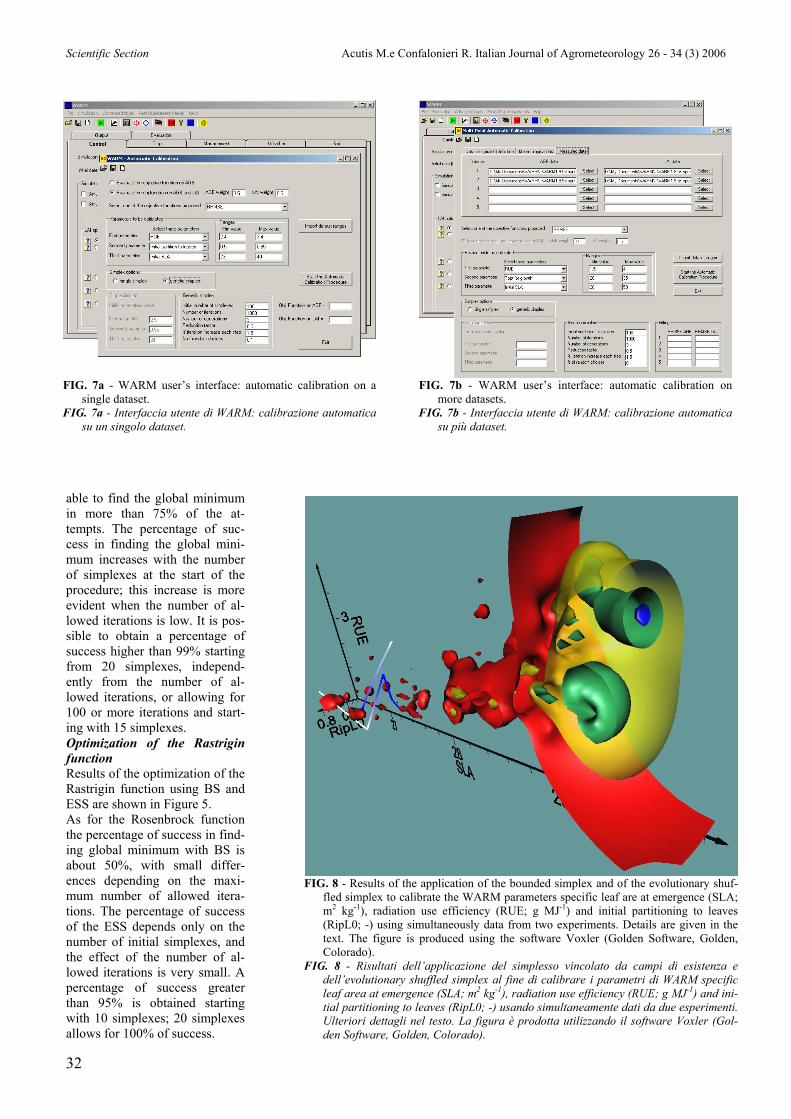
FIG. 8 - Results of the application of the bounded simplex and of the evolutionary shuf-

fled simplex to calibrate the WARM parameters specific leaf are at emergence (SLA; m2 kg-1), radiation use efficiency (RUE; g MJ-1) and initial partitioning to leaves (RipL0; -) using simultaneously data from two experiments. Details are given in the text. The figure is produced using the software Voxler (Golden Software, Golden, Colorado).

FIG. 8 - Risultati dell’applicazione del simplesso vincolato da campi di esistenza e dell’evolutionary shuffled simplex al fine di calibrare i parametri di WARM specific leaf area at emergence (SLA; m2 kg-1), radiation use efficiency (RUE; g MJ-1) and ini-tial partitioning to leaves (RipL0; -) usando simultaneamente dati da due esperimenti. Ulteriori dettagli nel testo. La figura è prodotta utilizzando il software Voxler (Gol-den Software, Golden, Colorado).


33

Implementation of the standard and evolu-tionary shuffled simplexes in the WARM model Figure 6 shows the fluxes of information involved with the implementation of the standard and evolutionary shuffled simplexes within the WARM modelling system (Confalonieri et al., 2005; Confalonieri et al., 2006a). Figure 7 shows the sections of the WARM user’s inter-face dedicated to the automatic calibration of crop model parameters using data from a single experiment (Figure 7.a) and from more experiments (up to five) (Figure 7.b). Figure 8 shows the results of the application of the two methods to calibrate the WARM parameters specific leaf area (SLA; m2 kg-1), radiation use efficiency (RUE; g MJ-1) and initial partitioning to leaves (RipL0; -) using simultaneously data from two experiments. The two datasets are described by Confalonieri et al. (2006b) and refer to the experiments carried out in Opera (northern Milan) during 2002 and 2004. In this example, the objec-tive function (relative root mean square error; %) was evaluated on above ground biomass separately for the two datasets. A composite objective function (COF; %) was then obtained adding the values of the RRMSEs computed for the two datasets. The axes refer to RUE, SLA, and RipL0. The blue ball in the up-right corner of the figure represents the global minimum (COF=46.5%) found by the evolutionary shuffled simplex (number of initial simplexes = 40; maximum number of iterations = 100; number of generations = 3). The red, yellow, and green surfaces represent areas in the space where COF assumes, respectively, the values of 49.2%, 48.0 %, and 47.3%. It is evident that values of COF very close to the best (46.5%) correspond to wide regions in the space generated by the three parameters under calibration. The red bubbles in the region close to the origin of the axes correspond to local minima. The two blue-white lines show the path of two standard simplexes which did not succeed in finding the global minimum. The starting guess for these two simplexes was in both cases inside the region of the space determined by the biophysical domain of each parameter under calibration. The colours of the two lines correspond to different values of COF: white in case of high COF values, blue in case of low COF values. It is evident that although in both cases the standard simplexes reach a satisfactory value of COF, they conclude their route inside two red bubbles which are very far from the global minimum. It is necessary to underline that other standard simplexes starting from different initial guesses reached the region of the space where the global minimum is located. Moreover, in the example reported in Figure 8, two dif-ferent datasets were simultaneously used for calibration. When a single experiment was used, the performances of the two optimization algorithms were comparable. The last consideration is about the time required by the two methods: the standard simplex usually reaches a re-sult in few steps (few tens of iterations) while the evolu-tionary shuffled simplex can require hundreds or thou-sands of iterations, according to its parameterization.

Conclusions It is possible to find in the literature many approaches and algorithms able to automatically calibrate parameters or variables of simulations models. However, no scien-tific evidence is known about the use of these powerful tools for calibrating crop models. In this work, the stan-dard downhill simplex and the evolutionary shuffled simplex, considered by the Authors particularly suitable for biophysical models, are briefly described and tested using two standard functions considered hard tests for optimization methods. If the hyperspace delimited by the parameters being calibrated is particularly complex, usu-ally the evolutionary shuffled simplex performs better. And this is often the case when biophysical models are calibrated using simultaneously data from different ex-periments. Of course, requirements in terms of iterations are completely different for the two algorithms and this should be taken into account before applying them. The implementation of the two simplex methods in the WARM simulation environment allows carrying out sin-gle- or multi-experiment calibrations in a really powerful and repeatable way. Although these optimization meth-ods are already used for calibrating simulation models in other disciplines, this is the first time they are used, and coupled, for calibrating a crop model. Free software components for COM and .NET environ-ments implementing both the discussed methods are un-der development. Acknowledgements This publication has been partially funded under the SEAMLESS integrated project, EU 6th Framework Pro-gramme for Research, Technological Development and Demonstration, Priority 1.1.6.3. Global Change and Eco-systems (European Commission, DG Research, contract no. 010036-2). References Beck, M.B., 1987. Water quality modeling: a review of the analysis of

uncertainty. Water Resour. Res., 23, 1393-1442. Bellocchi, G., Acutis, M., Fila, G., Donatelli, M. 2002. An indicator of

solar radiation model performances based on a fuzzy expert system. Agronomy Journal, 94, 1222-1233.

Brazil, L.E., 1988. Multilevel calibration strategy for complex hydro-logic simulation models. Ph.D. dissertation, Dep. Of Civ. Eng., Colo. State Univ., Fort Collins.

Confalonieri, R., Acutis, M., Donatelli, M., Bellocchi, G., Mariani, L., Boschetti, M., Stroppiana, D., Bocchi, S., Vidotto, F., Sacco, D., Gri-gnani, C., Ferrero, A., Genovese, G., 2005. WARM: A scientific group on rice modeling. Rivista Italiana di Agrometeorologia, 2, 54-60.

Confalonieri, R., Gusberti, D., Acutis, D., 2006a. Comparison of WO-FOST, CropSyst and WARM for simulating rice growth (Japonica type – short cycle varieties). Italian Journal of Agrometeorology, 3, 7-16

Confalonieri, R., Gusberti, D., Bocchi, S., Acutis, M., 2006b. The CropSyst model to simulate the N balance of rice for alternative management. Agronomy for Sustainable Development, 26,241-249.

Donatelli, M., Omicidi, A., Fila, G., Monti, C., 2004. Targeting reus-ability and replaceability of simulation models for agricultural sys-tems. Proc. 8th ESA Congress , 11-15 July, Copenhagen, Denmark,, 237-238.

Dorigo, M., 1992. Optimization, learning and natural algorithms. PhD thesis, Politecnico di Milano, Italy.

Duan, Q., Sorooshian, S., Gupta, V.K., 1992. Effective and efficient global optimization for conceptual rainfall runoff models. Water Re-sources Research, 28, 1015-1031.


34

Gan, T.Y., Biftu, G.F., 1996. Automatic calibration of conceptual rain-fall-runoff models: optimization algorithms, catchment conditions, and model structure. Water Resources Research, 32, 3513-3524.

Glover, F., 1986. Future paths for integer programming and links to artificial intelligence. Computers and Operations Research, 5, 533-549.

Holland, J.H., 1975. Adaptation in natural and artificial systems. University of Michigan Press, Ann Arbor.

Kirkpatrick, S., Gelatt, C.D., Vecchi, M.P., 1983. Optimization by simulated annealing. Science, 220, 671-680.

Kvasnička, V., Pospìchal, J., 1997. A hybrid of simplex method and simulated annealing. Chemometrics and Intelligent Laboratory Sys-tems, 39, 161-173.

Loague, K.M., Green, R.E., 1991. Statistical and graphical methods for evaluating solute transport models: overview and application. Jour-nal of Contaminant Hydrology, 7, 51-73

Martorana, F., Bellocchi, G., 1999. A review of methodologies to evaluate agroecosystem simulation models. Italian Journal of Agronomy, 3, 19-39.

Matsumoto, T., Du, H., Lindsey, J.S., 2002. A parallel simplex search method for use with an automated chemistry workstation. Chemom-etrics and Intelligent Laboratory Systems, 62, 129– 147.

Nelder, J.A., Mead, R., 1965. A simplex method for function minimiza-tion. Computer Journal, 7, 308-313.

Press, W.H., Teukolsky, S.A., Vetterling, W.T., Flannery, B.P., 1992. Numerical Recipes in C: the art of scientific computing, Second Edi-tion, Cambridge University Press, Cambridge.

Romano, N., Santini, A., 2002. Water retention and storage: Field. In Methods of Soil Analysis, part 4, Physical Methods (J.H. Dane and G.C. Topp, eds.), 721-738, SSSA Book Series N.5, Madison, WI, USA.

Rosenbrock, H.H., 1960. An automatic method for finding the greatest or least value of a function. Computer Journal, 3, 175-184.

Smyth, G.K., 2002. Optimization. In Encyclopedia of Environmetrics, Vol. 3 (A.H. El-Shaarawi and W.W. Piegorsch), 1481-1487, John Wiley & Sons, Chichester.

Smith, P., Smith, J.U., Powlson, D.S., McGill, W.B., Arah, J.R.M., Chertov, O.G., Coleman, K., Franko, U., Frolking, S., Jenkinson, D.S., Jensen, L.S., Kelly, R.H., Klein-Gunnewiek, H., Komarov, A.S., Li, C., Molina, J.A.E., Mueller, T., Parton, W.J., Thornley, J.H.M., Whitmore, A.P., 1997. A comparison of the performance of nine soil organic matter models using datasets from seven long-term experi-ments. Geoderma, 81, 153-225.

Tedeschi, L.O., 2005. Assessment of the adequacy of mathematical models. Agr. Syst., 89, 225-247.

Törn, A., Zilinskas, A., 1989. Global optimization. Lecture Notes in Computer Science, N° 350, Springer-Verlag, Berlin.

. .

ALGORITMI DI OTTIMIZZAZIONE PER LA CALIBRAZIONE DI … · Scientific Section Acutis M.e...

Documents

Transcript of ALGORITMI DI OTTIMIZZAZIONE PER LA CALIBRAZIONE DI … · Scientific Section Acutis M.e...