AlgorithmsFreely using the textbook by Cormen, Leiserson, Rivest, Stein

Péter Gács

Computer Science DepartmentBoston University

Fall 2010

The class structure

See the course homepage.In the notes, section numbers and titles generally refer to the book:CLSR: Algorithms, third edition.

Algorithms

Computational problem example: sorting.Input, output, instance.

Algorithm example: insertion sort.

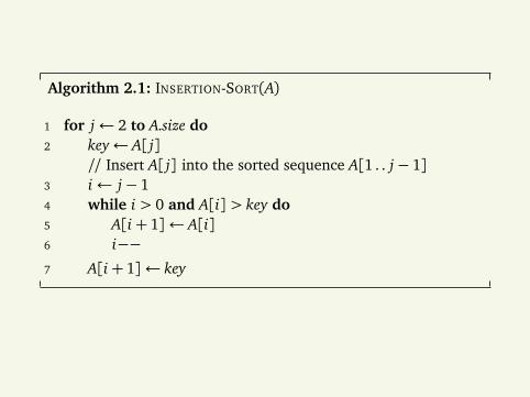
Algorithm 2.1: INSERTION-SORT(A)

1 for j← 2 to A.size do2 key← A[ j]

// Insert A[ j] into the sorted sequence A[1 . . j− 1]3 i← j− 14 while i > 0 and A[i]> key do5 A[i+ 1]← A[i]6 i−−7 A[i+ 1]← key

Pseudocode conventions

Assignment

Indentation

Objects Arrays are also objects.Meaning of A[3 . . 10].

Parameters Ordinary parameters are passed by value.Objects are always treated like a pointer to the body of data,which themselves are not copied.

Analyzing algorithms

By size of a problem, we will mean the size of its input (measuredin bits).

Cost as function of input size. In a problem of fixed size, the costwill be influenced by too many accidental factors: this makes ithard to draw lessons applicable to future cases.

Our model for computation cost: Random Access Machine Untilfurther refinement, one array access is assumed to take constantamount of time (independent of input size or array size).

Resources: running time, memory, communication (in case ofseveral processors or actors).

Estimating running time

When a program line involves only a simple instruction weassume it has constant cost. The main question is the numberof times it will be executed. It is better to think in terms oflarger program parts than in terms of program lines.

If a part is a loop then the time is the overhead plus the sum ofthe execution times for each repetition.

If a part is a conditonal then the time depends on which branchis taken.

And so on.

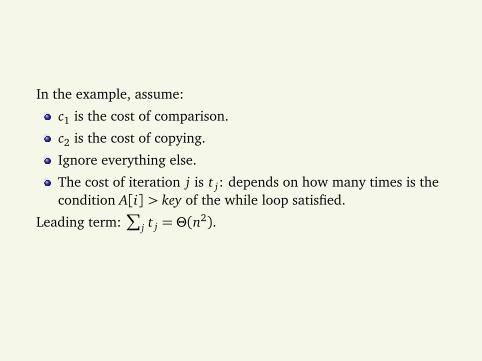
In the example, assume:

c1 is the cost of comparison.

c2 is the cost of copying.

Ignore everything else.

The cost of iteration j is t j: depends on how many times is thecondition A[i]> key of the while loop satisfied.

Leading term:∑

j t j =Θ(n2).

Data structures

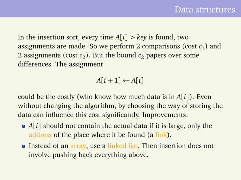
In the insertion sort, every time A[i]> key is found, twoassignments are made. So we perform 2 comparisons (cost c1) and2 assignments (cost c2). But the bound c2 papers over somedifferences. The assignment

A[i+ 1]← A[i]

could be the costly (who know how much data is in A[i]). Evenwithout changing the algorithm, by choosing the way of storing thedata can influence this cost significantly. Improvements:

A[i] should not contain the actual data if it is large, only theaddress of the place where it be found (a link).

Instead of an array, use a linked list. Then insertion does notinvolve pushing back everything above.

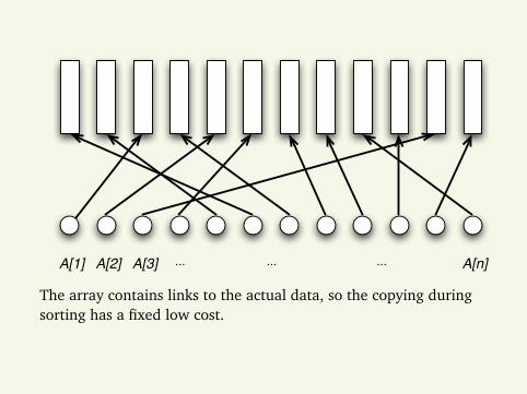
A[1] A[2] A[3] ... ... ... A[n]

The array contains links to the actual data, so the copying duringsorting has a fixed low cost.

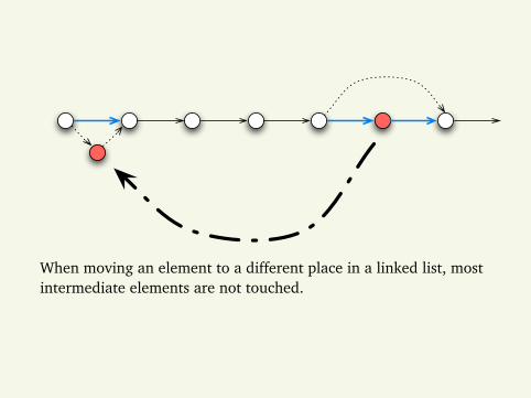
When moving an element to a different place in a linked list, mostintermediate elements are not touched.

Worst case, average case

Worst case We estimated the largest cost of an algorithm for agiven input size. This is what we will normally do.

Average case What does this mean?The notion of a random, or typical input is problematic.But we can introduce random choices in our algorithm, bya process called randomization. We will see exampleswhen this can give an average performance significantlybetter than the worst-case performance, on all inputs.

Strong and weak domination

For the insertion sort, in first approximation, we just want to knowthat its worst-case cost “grows as” n2, where n is the file size. Inyour introductory courses CS112 and CS131 you already have seenthe basic notions needed to talk about this “grows as”. Here, Icollect some this information: more is found here than what I havetime for initially in class.

Rough comparison of functions

f (n) g(n) means limn→∞ f (n)/g(n) = 0: in words, g(n) growsfaster than f (n). Other notation:

f (n) = o(g(n))⇔ f (n) g(n)⇔ g(n) =ω( f (n)).

Example: n− 4 116p

n+ 80. We may also write

116p

n+ 80= o(n).

Generally, when we write f (n) = o(g(n)) then g(n) has a simplerform than f (n) (this is the point of the notation).

f (n)∗< g(n) means supn f (n)/g(n)<∞, that is f (n)¶ c · g(n) for

some constant c. Other (the common) notation:

f (n) = O(g(n))⇔ f (n)∗< g(n)⇔ g(n) = Ω( f (n)).

(The notation∗< is mine, you will not find it in your books.)

This is a preorder. If f∗< g and g

∗< f then we write f ∗= g,

f =Θ(g), and say that f and g have the same rate of growth.Example: n2− 5n and 100n(n+ 2) have the same rate of growth.We can also write

100n(n+ 2) = O(n2), 100n(n+ 2) = Θ(n2).

On the other hand, n+p

n= O(n2) but not Θ(n2).

Important special cases

O(1) denotes any function that is bounded by a constant, forexample (1+ 1/n)n = O(1).

o(1) denotes any function that is converging to 0 as n→∞. Forexample, another way of writing Stirling’s formula is

n!=n

e

np2πn(1+ o(n)).

Not all pairs of functions are comparable

Here are two functions that are not comparable. Let f (n) = n2, andfor k = 0, 1,2, . . . , we define g(n) recursively as follows. Let nk bethe sequence defined by n0 = 1, nk+1 = 2nk . So, n1 = 2, n2 = 4,n3 = 16, and so on. For k = 1, 2, . . . let

g(n) = nk+1 if nk < n¶ nk+1.

So,g(nk + 1) = nk+1 = 2nk = g(nk + 1) = g(nk + 2) = · · ·= g(nk+1).This gives g(n) = 2n−1 for n= nk + 1 and g(n) = n for n= nk+1.Function g(n) is sometimes much bigger than f (n) = n2 andsometimes much smaller: these functions are incomparable for,

∗<.

Some function classes

Important classes of increasing functions of n:

Linear functions: (bounded by) c · n for arbitrary constant c.

Polynomial functions: (bounded by) nc for some constant c > 0,for n¾ 2.

Exponential functions: those (bounded by) cn for someconstant c > 1.

Logarithmic functions: (bounded by) c · log n for arbitraryconstant c. Note: If a function is logarithmic with log2 then it isalso logarithmic with logb for any b, since

logb x =log2 x

log2 b= (log2 x)(logb 2).

These are all equivalence classes under ∗=.

Some simplification rules

Addition: take the maximum, that is if f = O(g) thenf + g = O(g). Do this always to simplify expressions.Warning: do it only if the number of terms is constant! This iswrong: n+ n+ · · · (n times) · · ·+ n 6= O(n).

f (n)g(n) is generally worth rewriting as 2g(n) log f (n). Forexample, nlog n = 2(log n)·(log n) = 2log2 n.

But sometimes we make the reverse transformation:

3log n = 2(log n)·(log 3) = (2log n)log3 = nlog 3.

The last form is the most meaningful, showing that this is apolynomial function.

Examples

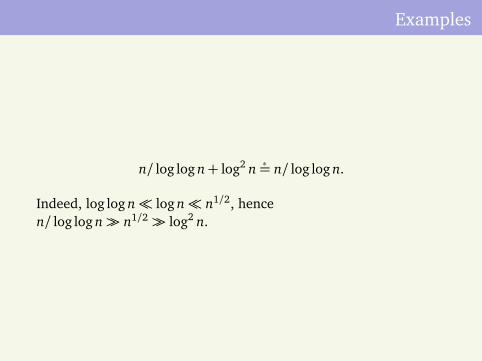
n/ log log n+ log2 n ∗= n/ log log n.

Indeed, log log n log n n1/2, hencen/ log log n n1/2 log2 n.

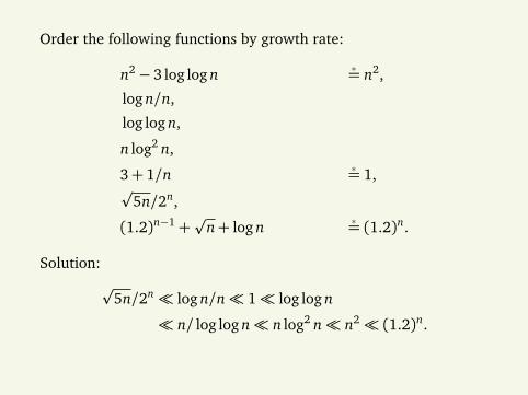
Order the following functions by growth rate:

n2− 3 log log n ∗= n2,

log n/n,

log log n,

n log2 n,

3+ 1/n ∗= 1,p5n/2n,

(1.2)n−1+p

n+ log n ∗= (1.2)n.

Solution:p

5n/2n log n/n 1 log log n

n/ log log n n log2 n n2 (1.2)n.

Sums of series

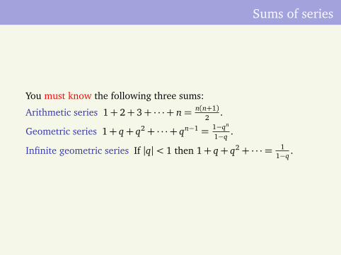
You must know the following three sums:

Arithmetic series 1+ 2+ 3+ · · ·+ n= n(n+1)2

.

Geometric series 1+ q+ q2+ · · ·+ qn−1 = 1−qn

1−q.

Infinite geometric series If |q|< 1 then 1+ q+ q2+ · · ·= 11−q

.

Simplification of sums

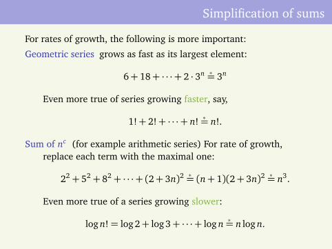
For rates of growth, the following is more important:

Geometric series grows as fast as its largest element:

6+ 18+ · · ·+ 2 · 3n ∗= 3n

Even more true of series growing faster, say,

1!+ 2!+ · · ·+ n! ∗= n!.

Sum of nc (for example arithmetic series) For rate of growth,replace each term with the maximal one:

22+ 52+ 82+ · · ·+ (2+ 3n)2 ∗= (n+ 1)(2+ 3n)2 ∗= n3.

Even more true of a series growing slower:

log n!= log2+ log3+ · · ·+ log n ∗= n log n.

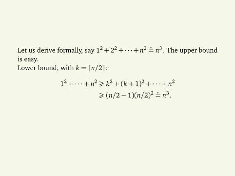
Let us derive formally, say 12+22+ · · ·+ n2 ∗= n3. The upper boundis easy.Lower bound, with k = dn/2e:

12+ · · ·+ n2 ¾ k2+ (k+ 1)2+ · · ·+ n2

¾ (n/2− 1)(n/2)2 ∗= n3.

Infinite series

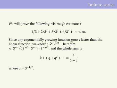
We will prove the following, via rough estimates:

1/3+ 2/32+ 3/33+ 4/34+ · · ·<∞.

Since any exponentially growing function grows faster than thelinear function, we know n

∗< 3n/2. Therefore

n · 3−n ∗< 3n/2 · 3−n = 3−n/2, and the whole sum is

∗< 1+ q+ q2+ · · ·= 1

1− q

where q = 3−1/2.

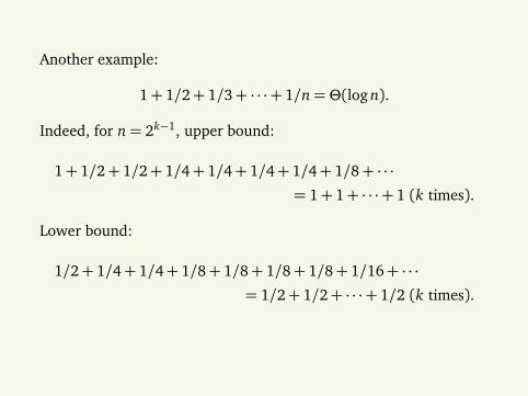
Another example:

1+ 1/2+ 1/3+ · · ·+ 1/n=Θ(log n).

Indeed, for n= 2k−1, upper bound:

1+ 1/2+ 1/2+ 1/4+ 1/4+ 1/4+ 1/4+ 1/8+ · · ·= 1+ 1+ · · ·+ 1 (k times).

Lower bound:

1/2+ 1/4+ 1/4+ 1/8+ 1/8+ 1/8+ 1/8+ 1/16+ · · ·= 1/2+ 1/2+ · · ·+ 1/2 (k times).

Divide and conquer

An efficient algorithm can frequently obtained using the followingidea:

1 Divide into subproblems of equal size.2 Solve subproblems.3 Combine results.

In order to handle subproblems, a more general procedure is oftenneeded.

Merge sort

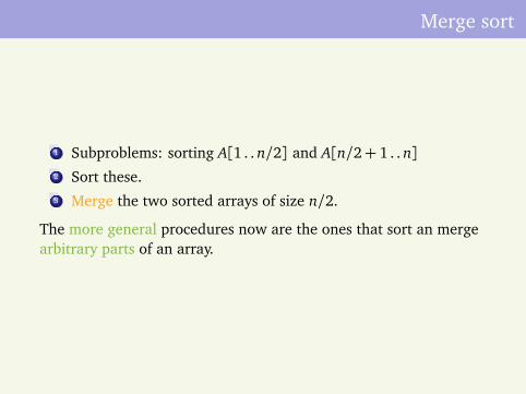
1 Subproblems: sorting A[1 . . n/2] and A[n/2+ 1 . . n]2 Sort these.3 Merge the two sorted arrays of size n/2.

The more general procedures now are the ones that sort an mergearbitrary parts of an array.

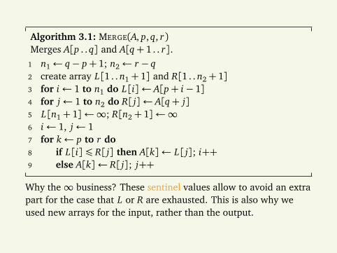
Algorithm 3.1: MERGE(A, p, q, r)Merges A[p . . q] and A[q+ 1 . . r].

1 n1← q− p+ 1; n2← r − q2 create array L[1 . . n1+ 1] and R[1 . . n2+ 1]3 for i← 1 to n1 do L[i]← A[p+ i− 1]4 for j← 1 to n2 do R[ j]← A[q+ j]5 L[n1+ 1]←∞; R[n2+ 1]←∞6 i← 1, j← 17 for k← p to r do8 if L[i]¶ R[ j] then A[k]← L[ j]; i++9 else A[k]← R[ j]; j++

Why the∞ business? These sentinel values allow to avoid an extrapart for the case that L or R are exhausted. This is also why weused new arrays for the input, rather than the output.

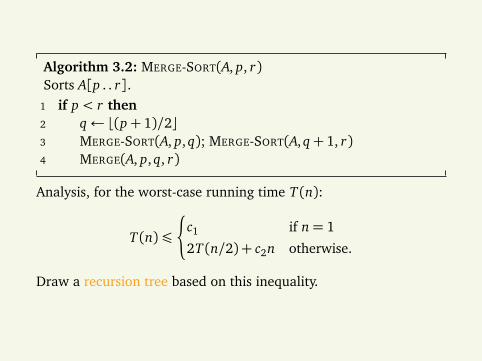
Algorithm 3.2: MERGE-SORT(A, p, r)Sorts A[p . . r].

1 if p < r then2 q← b(p+ 1)/2c3 MERGE-SORT(A, p, q); MERGE-SORT(A, q+ 1, r)4 MERGE(A, p, q, r)

Analysis, for the worst-case running time T (n):

T (n)¶

(

c1 if n= 1

2T (n/2) + c2n otherwise.

Draw a recursion tree based on this inequality.

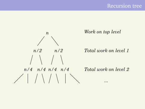
Recursion tree

n

n/2 n/2

n/4 n/4 n/4 n/4

Work on top level

Total work on level 1

Total work on level 2

...

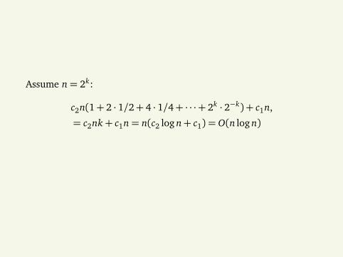
Assume n= 2k:

c2n(1+ 2 · 1/2+ 4 · 1/4+ · · ·+ 2k · 2−k) + c1n,

= c2nk+ c1n= n(c2 log n+ c1) = O(n log n)

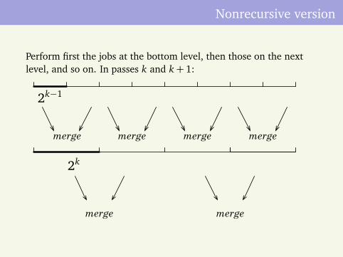
Nonrecursive version

Perform first the jobs at the bottom level, then those on the nextlevel, and so on. In passes k and k+ 1:

merge merge merge merge

2k−1

2k

merge merge

Sorting without random access

What if we have to sort such a large list A, that it does not fitinto random access memory?

If we are at a position p we can inspect or change A[p], but inone step, we can only move to position p+ 1 or p− 1.

Note that the Algorithm MERGE(A, p, q, r) passed through arraysA, L, R in one direction only, not jumping around. But both therecursive and nonrecursive MERGE-SORT(A) uses random access.

We will modify the nonrecursive MERGE-SORT(A) to workwithout random access.

Runs

For position p in array A, let p′ ¾ p be as large as possible with

A[p]¶ A[p+ 1]¶ · · ·¶ A[p′].

The sub-array A[p . . p′] will be called a run.Our algorithm will consist of a number of passes. Each pass goesthrough array A and merges consecutive runs: namely

performs MERGE(A, p, q, r) where p = 1, q = p′, r = (q+ 1)′,does the same starting with p← r + 1

and so on.

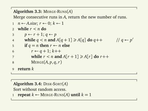
Algorithm 3.3: MERGE-RUNS(A)Merge consecutive runs in A, return the new number of runs.

1 n← A.size; r ← 0; k← 12 while r < n do3 p← r + 1; q← p4 while q < n and A[q+ 1]¾ A[q] do q++ // q← p′

5 if q = n then r ← n else6 r ← q+ 1; k++7 while r < n and A[r + 1]¾ A[r] do r++8 MERGE(A, p, q, r)

9 return k

Algorithm 3.4: DISK-SORT(A)Sort without random access.

1 repeat k←MERGE-RUNS(A) until k = 1

Each MERGE-RUNS(A) roughly halves the number of runs.

If you view the arrays as being on tapes, the algorithm uses stilltoo many rewind operations to return from the end of the tapeto the beginning. In an exercise, I will ask you to modifyDISK-SORT(A) (and MERGE-RUNS(A)) to so as to eliminate almostall rewinds.

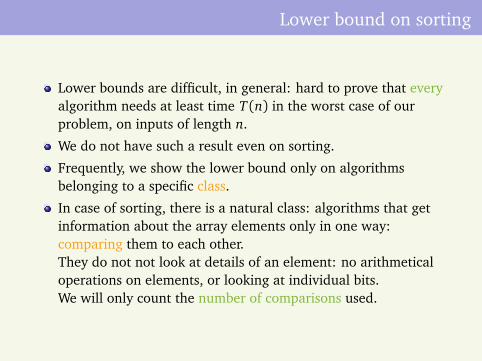
Lower bound on sorting

Lower bounds are difficult, in general: hard to prove that everyalgorithm needs at least time T (n) in the worst case of ourproblem, on inputs of length n.

We do not have such a result even on sorting.

Frequently, we show the lower bound only on algorithmsbelonging to a specific class.

In case of sorting, there is a natural class: algorithms that getinformation about the array elements only in one way:comparing them to each other.They do not not look at details of an element: no arithmeticaloperations on elements, or looking at individual bits.We will only count the number of comparisons used.

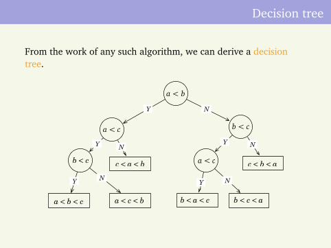
Decision tree

From the work of any such algorithm, we can derive a decisiontree.

b < c

a < b < c a < c < b

c < a < b

b < a < c b < c < a

c < b < a

NY

Y NY N

Y NY N

a < b

a < c b < c

a < c

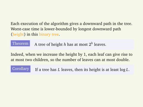
Each execution of the algorithm gives a downward path in the tree.Worst-case time is lower-bounded by longest downward path(height) in this binary tree.

Theorem A tree of height h has at most 2h leaves.

Indeed, when we increase the height by 1, each leaf can give rise toat most two children, so the number of leaves can at most double.

Corollary If a tree has L leaves, then its height is at least log L.

Application to sorting

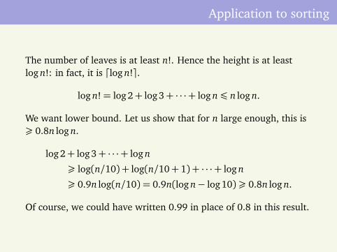
The number of leaves is at least n!. Hence the height is at leastlog n!: in fact, it is dlog n!e.

log n!= log2+ log 3+ · · ·+ log n¶ n log n.

We want lower bound. Let us show that for n large enough, this is¾ 0.8n log n.

log2+ log3+ · · ·+ log n

¾ log(n/10) + log(n/10+ 1) + · · ·+ log n

¾ 0.9n log(n/10) = 0.9n(log n− log10)¾ 0.8n log n.

Of course, we could have written 0.99 in place of 0.8 in this result.

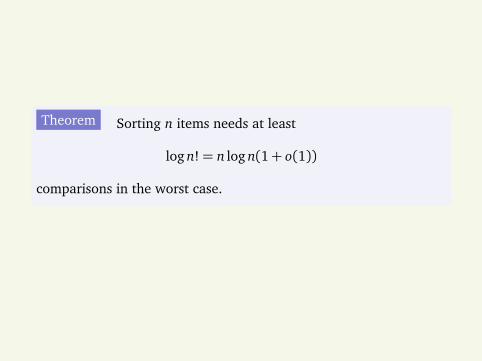
Theorem Sorting n items needs at least

log n!= n log n(1+ o(1))

comparisons in the worst case.

Average case

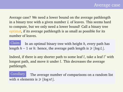
Average case? We need a lower bound on the average pathlengthin a binary tree with a given number L of leaves. This seems hardto compute, but we only need a lower bound! Call a binary treeoptimal, if its average pathlength is as small as possible for itsnumber of leaves.

Claim In an optimal binary tree with height h, every path haslength h− 1 or h: hence, the average path length is ¾ blog Lc.

Indeed, if there is any shorter path to some leaf l, take a leaf l ′ withlongest path, and move it under l. This decreases the averagepathlength.

Corollary The average number of comparisons on a random listwith n elements is ¾ blog n!c.

Information

Here is an intuitive retelling of the above argument.If all we know about an object x is that it belongs to some knownset E of size m, we say that we have an uncertainty of size log m (mbits). Each comparison gives us at most 1 bit of information(decrease of uncertainty) about the permutation in question. Sincethere are n! permutations, our uncertainty is log n!, so we needthat many bits of information to remove it.

Finding the maximum

Here is another decision-tree lower bound, that is notinformation-theoretic.

Problem Given a list of n numbers, find the largest element.

Solution (You know it: one pass.)

Other solution Tournament.

Cost n− 1 comparisons in both cases.

Question Is this optimal?

The information-theoretical lower bound is log n.

Theorem We need at least n− 1 comparisons in order to findthe maximum.

Indeed, every non-maximum element must participate in acomparison that shows it is smaller than the one it is compared to.

Listing permutations

Here is another algorithm that is guaranteed to take a long time:list all permutations of an array.

Why is it taking long? For a trivial reason: the output is long (n! · nitems).

How to implement? It is not so easy to organize going through allpossibilities. We will use recursion: similar techniques will helpwith other problems involving exhaustive search.

In what order to list? Lexicographical order: If a1 . . . ak . . . an andb1 . . . bk . . . bn are permutations, ai = bi for i < k and ak < bkthen a1 . . . ak . . . an comes first.

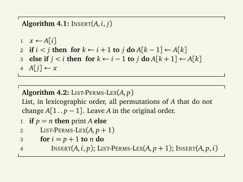
Algorithm 4.1: INSERT(A, i, j)

1 x ← A[i]2 if i < j then for k← i+ 1 to j do A[k− 1]← A[k]3 else if j < i then for k← i− 1 to j do A[k+ 1]← A[k]4 A[ j]← x

Algorithm 4.2: LIST-PERMS-LEX(A, p)List, in lexicographic order, all permutations of A that do notchange A[1 . . p− 1]. Leave A in the original order.

1 if p = n then print A else2 LIST-PERMS-LEX(A, p+ 1)3 for i = p+ 1 to n do4 INSERT(A, i, p); LIST-PERMS-LEX(A, p+ 1); INSERT(A, p, i)

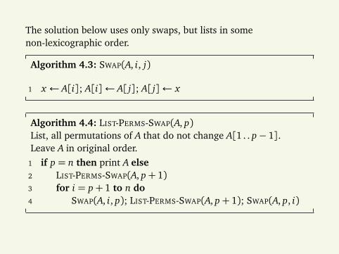
The solution below uses only swaps, but lists in somenon-lexicographic order.

Algorithm 4.3: SWAP(A, i, j)

1 x ← A[i]; A[i]← A[ j]; A[ j]← x

Algorithm 4.4: LIST-PERMS-SWAP(A, p)List, all permutations of A that do not change A[1 . . p− 1].Leave A in original order.

1 if p = n then print A else2 LIST-PERMS-SWAP(A, p+ 1)3 for i = p+ 1 to n do4 SWAP(A, i, p); LIST-PERMS-SWAP(A, p+ 1); SWAP(A, p, i)

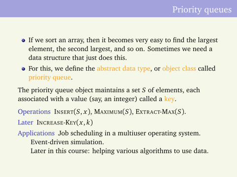
Priority queues

If we sort an array, then it becomes very easy to find the largestelement, the second largest, and so on. Sometimes we need adata structure that just does this.

For this, we define the abstract data type, or object class calledpriority queue.

The priority queue object maintains a set S of elements, eachassociated with a value (say, an integer) called a key.

Operations INSERT(S, x), MAXIMUM(S), EXTRACT-MAX(S).

Later INCREASE-KEY(x , k)

Applications Job scheduling in a multiuser operating system.Event-driven simulation.Later in this course: helping various algorithms to use data.

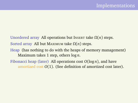
Implementations

Unordered array All operations but INSERT take Ω(n) steps.

Sorted array All but MAXIMUM take Ω(n) steps.

Heap (has nothing to do with the heaps of memory management)Maximum takes 1 step, others log n.

Fibonacci heap (later) All operations cost O(log n), and haveamortized cost O(1). (See definition of amortized cost later).

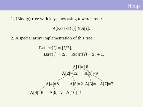
Heap

1. (Binary) tree with keys increasing towards root:

A[PARENT(i)]¾ A[i].

2. A special array implementation of this tree:

PARENT(i) = bi/2c,LEFT(i) = 2i, RIGHT(i) = 2i+ 1.

A[1]=15A[2]=12 A[3]=9

A[4]=8 A[5]=2 A[6]=1 A[7]=7

A[8]=6 A[9]=7 A[10]=1

Building and maintaining a heap

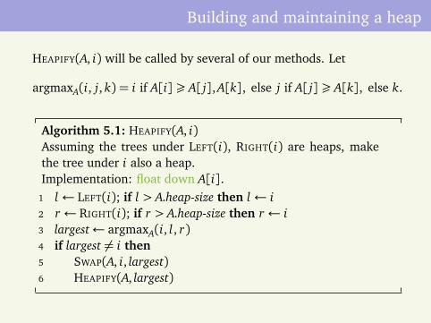
HEAPIFY(A, i) will be called by several of our methods. Let

argmaxA(i, j, k) = i if A[i]¾ A[ j], A[k], else j if A[ j]¾ A[k], else k.

Algorithm 5.1: HEAPIFY(A, i)Assuming the trees under LEFT(i), RIGHT(i) are heaps, makethe tree under i also a heap.Implementation: float down A[i].

1 l ← LEFT(i); if l > A.heap-size then l ← i2 r ← RIGHT(i); if r > A.heap-size then r ← i3 largest← argmaxA(i, l, r)4 if largest 6= i then5 SWAP(A, i, largest)6 HEAPIFY(A, largest)

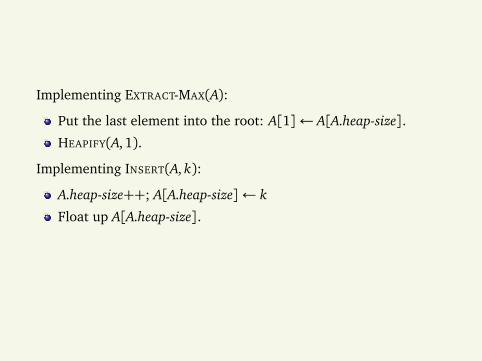
Implementing EXTRACT-MAX(A):

Put the last element into the root: A[1]← A[A.heap-size].

HEAPIFY(A, 1).

Implementing INSERT(A, k):

A.heap-size++; A[A.heap-size]← k

Float up A[A.heap-size].

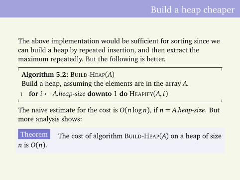
Build a heap cheaper

The above implementation would be sufficient for sorting since wecan build a heap by repeated insertion, and then extract themaximum repeatedly. But the following is better.

Algorithm 5.2: BUILD-HEAP(A)Build a heap, assuming the elements are in the array A.

1 for i← A.heap-size downto 1 do HEAPIFY(A, i)

The naive estimate for the cost is O(n log n), if n= A.heap-size. Butmore analysis shows:

Theorem The cost of algorithm BUILD-HEAP(A) on a heap of sizen is O(n).

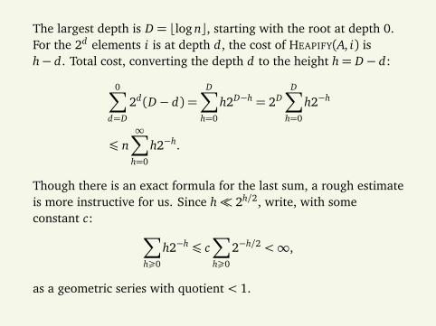
The largest depth is D = blog nc, starting with the root at depth 0.For the 2d elements i is at depth d, the cost of HEAPIFY(A, i) ish− d. Total cost, converting the depth d to the height h= D− d:

0∑

d=D

2d(D− d) =D∑

h=0

h2D−h = 2DD∑

h=0

h2−h

¶ n∞∑

h=0

h2−h.

Though there is an exact formula for the last sum, a rough estimateis more instructive for us. Since h 2h/2, write, with someconstant c:

∑

h¾0

h2−h ¶ c∑

h¾0

2−h/2 <∞,

as a geometric series with quotient < 1.

Abstract data types (objects)

Some pieces of data, together with some operations that can beperformed on them.

Externally, only the operations are given, and only these shouldbe accessible to other parts of the program.

The internal representation is private. It consists typically of anumber of records, where each record has key, satellite data.We will ignore the satellite data unless they are needed for thedata manipulation itself.

Increasing a key

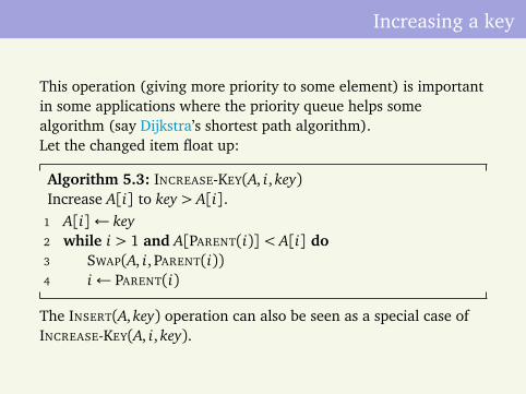
This operation (giving more priority to some element) is importantin some applications where the priority queue helps somealgorithm (say Dijkstra’s shortest path algorithm).Let the changed item float up:

Algorithm 5.3: INCREASE-KEY(A, i, key)Increase A[i] to key > A[i].

1 A[i]← key2 while i > 1 and A[PARENT(i)]< A[i] do3 SWAP(A, i, PARENT(i))4 i← PARENT(i)

The INSERT(A, key) operation can also be seen as a special case ofINCREASE-KEY(A, i, key).

Quicksort

Another way to apply “divide and conquer” to sorting. Both hereand in mergesort, we sort the two parts separately and combine theresults.

With Mergesort, we sort first two predetermined halves, andcombine the results later.

With Quicksort, we determine what elements fall into two“halves” (approximately) of the sorted result, using Partition.Calling this recursively on both “halves” completes the sort.

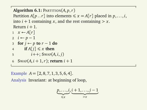
Algorithm 6.1: PARTITION(A, p, r)Partition A[p . . r] into elements ¶ x = A[r] placed in p, . . . , i,into i+ 1 containing x , and the rest containing > x .Return i+ 1.

1 x ← A[r]2 i← p− 13 for j← p to r − 1 do4 if A[ j]¶ x then5 i++; SWAP(A, i, j)

6 SWAP(A, i+ 1, r); return i+ 1

Example A= [2,8, 7,1, 3,5, 6,4].

Analysis Invariant: at beginning of loop,

p, . . . , i︸ ︷︷ ︸

¶x

, i+ 1, . . . , j− 1︸ ︷︷ ︸

>x

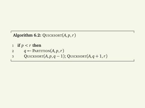
Algorithm 6.2: QUICKSORT(A, p, r)

1 if p < r then2 q← PARTITION(A, p, r)3 QUICKSORT(A, p, q− 1); QUICKSORT(A, q+ 1, r)

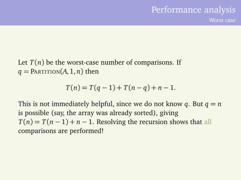
Performance analysisWorst case

Let T (n) be the worst-case number of comparisons. Ifq = PARTITION(A, 1, n) then

T (n) = T (q− 1) + T (n− q) + n− 1.

This is not immediately helpful, since we do not know q. But q = nis possible (say, the array was already sorted), givingT (n) = T (n− 1) + n− 1. Resolving the recursion shows that allcomparisons are performed!

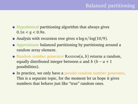
Balanced partitioning

Hypothetical partitioning algorithm that always gives0.1n< q < 0.9n.

Analysis with recursion tree gives n log n/ log(10/9).

Approximate balanced partitioning by partitioning around arandom array element.

Random number generator RANDOM(a, b) returns a random,equally distributed integer between a and b (b− a+ 1possibilities).

In practice, we only have a pseudo-random number generator.This is a separate topic, for the moment let us hope it givesnumbers that behave just like “true” random ones.

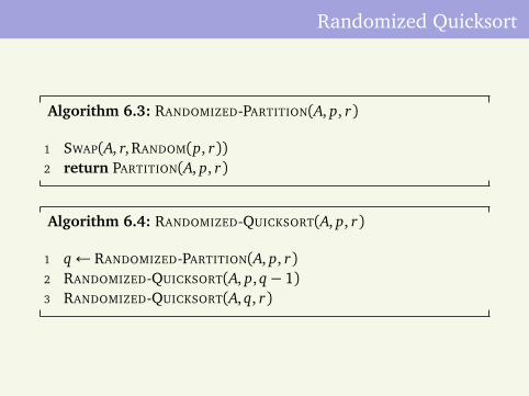
Randomized Quicksort

Algorithm 6.3: RANDOMIZED-PARTITION(A, p, r)

1 SWAP(A, r, RANDOM(p, r))2 return PARTITION(A, p, r)

Algorithm 6.4: RANDOMIZED-QUICKSORT(A, p, r)

1 q← RANDOMIZED-PARTITION(A, p, r)2 RANDOMIZED-QUICKSORT(A, p, q− 1)3 RANDOMIZED-QUICKSORT(A, q, r)

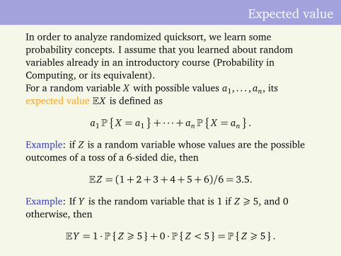
Expected value

In order to analyze randomized quicksort, we learn someprobability concepts. I assume that you learned about randomvariables already in an introductory course (Probability inComputing, or its equivalent).For a random variable X with possible values a1, . . . , an, itsexpected value EX is defined as

a1 P

X = a1

+ · · ·+ an P

X = an

.

Example: if Z is a random variable whose values are the possibleoutcomes of a toss of a 6-sided die, then

EZ = (1+ 2+ 3+ 4+ 5+ 6)/6= 3.5.

Example: If Y is the random variable that is 1 if Z ¾ 5, and 0otherwise, then

EY = 1 · P Z ¾ 5 + 0 · P Z < 5 = P Z ¾ 5 .

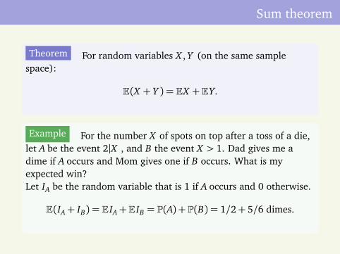
Sum theorem

Theorem For random variables X , Y (on the same samplespace):

E(X + Y ) = EX +EY.

Example For the number X of spots on top after a toss of a die,let A be the event 2|X , and B the event X > 1. Dad gives me adime if A occurs and Mom gives one if B occurs. What is myexpected win?Let IA be the random variable that is 1 if A occurs and 0 otherwise.

E(IA+ IB) = E IA+E IB = P(A) + P(B) = 1/2+ 5/6 dimes.

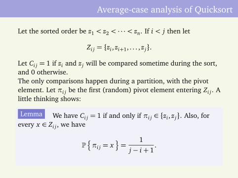
Average-case analysis of Quicksort

Let the sorted order be z1 < z2 < · · ·< zn. If i < j then let

Zi j = zi , zi+1, . . . , z j.

Let Ci j = 1 if zi and z j will be compared sometime during the sort,and 0 otherwise.The only comparisons happen during a partition, with the pivotelement. Let πi j be the first (random) pivot element entering Zi j . Alittle thinking shows:

Lemma We have Ci j = 1 if and only if πi j ∈ zi , z j. Also, forevery x ∈ Zi j , we have

P¦

πi j = x©

=1

j− i+ 1.

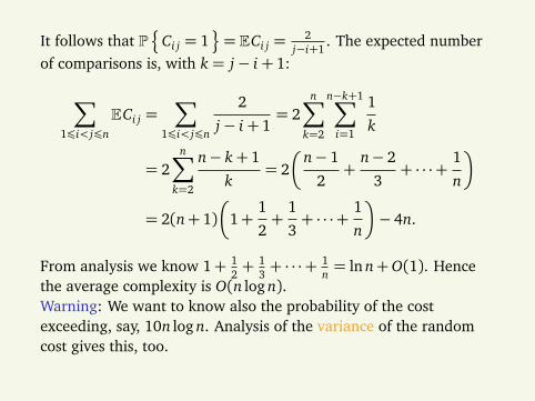
It follows that P¦

Ci j = 1©

= ECi j =2

j−i+1. The expected number

of comparisons is, with k = j− i+ 1:

∑

1¶i< j¶n

ECi j =∑

1¶i< j¶n

2

j− i+ 1= 2

n∑

k=2

n−k+1∑

i=1

1

k

= 2n∑

k=2

n− k+ 1

k= 2

n− 1

2+

n− 2

3+ · · ·+ 1

n

= 2(n+ 1)

1+1

2+

1

3+ · · ·+ 1

n

− 4n.

From analysis we know 1+ 12+ 1

3+ · · ·+ 1

n= ln n+O(1). Hence

the average complexity is O(n log n).Warning: We want to know also the probability of the costexceeding, say, 10n log n. Analysis of the variance of the randomcost gives this, too.

Median and order statistics

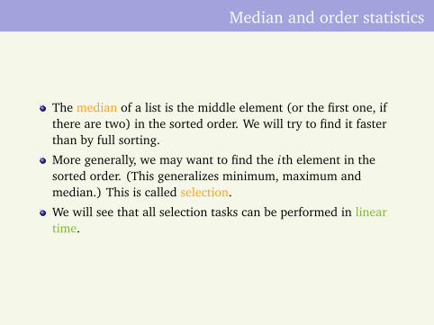
The median of a list is the middle element (or the first one, ifthere are two) in the sorted order. We will try to find it fasterthan by full sorting.

More generally, we may want to find the ith element in thesorted order. (This generalizes minimum, maximum andmedian.) This is called selection.

We will see that all selection tasks can be performed in lineartime.

Selection in expected linear time

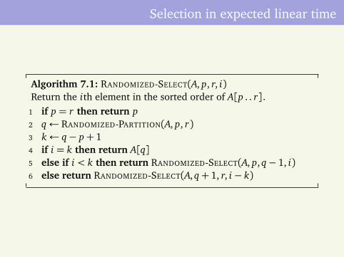
Algorithm 7.1: RANDOMIZED-SELECT(A, p, r, i)Return the ith element in the sorted order of A[p . . r].

1 if p = r then return p2 q← RANDOMIZED-PARTITION(A, p, r)3 k← q− p+ 14 if i = k then return A[q]5 else if i < k then return RANDOMIZED-SELECT(A, p, q− 1, i)6 else return RANDOMIZED-SELECT(A, q+ 1, r, i− k)

Analysis

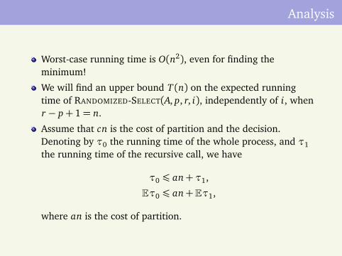
Worst-case running time is O(n2), even for finding theminimum!

We will find an upper bound T (n) on the expected runningtime of RANDOMIZED-SELECT(A, p, r, i), independently of i, whenr − p+ 1= n.

Assume that cn is the cost of partition and the decision.Denoting by τ0 the running time of the whole process, and τ1the running time of the recursive call, we have

τ0 ¶ an+τ1,

Eτ0 ¶ an+Eτ1,

where an is the cost of partition.

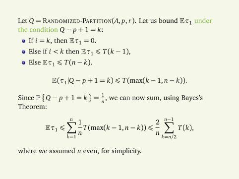
Let Q = RANDOMIZED-PARTITION(A, p, r). Let us bound Eτ1 underthe condition Q− p+ 1= k:

If i = k, then Eτ1 = 0.

Else if i < k then Eτ1 ¶ T (k− 1),

Else Eτ1 ¶ T (n− k).

E(τ1|Q− p+ 1= k)¶ T (max(k− 1, n− k)).

Since P

Q− p+ 1= k

= 1n, we can now sum, using Bayes’s

Theorem:

Eτ1 ¶n∑

k=1

1

nT (max(k− 1, n− k))¶

2

n

n−1∑

k=n/2

T (k),

where we assumed n even, for simplicity.

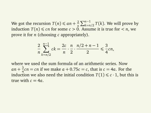
We got the recursion T (n)¶ an+ 2n

∑n−1k=n/2 T (k). We will prove by

induction T (n)¶ cn for some c > 0. Assume it is true for < n, weprove it for n (choosing c appropriately).

2

n

n−1∑

k=n/2

ck =2c

n· n

2· n/2+ n− 1

2¶

3

4cn,

where we used the sum formula of an arithmetic series. Nowan+ 3

4cn= cn if we make a+ 0.75c = c, that is c = 4a. For the

induction we also need the initial condition T (1)¶ c · 1, but this istrue with c = 4a.

Number-theoretic algorithms

Size of input Just as before, we count the number of input bits. Ifthe input is a positive integer x of 1000 bits, the input size is1000= dlog xe, and not x . So, counting from x down to 1 isan exponential algorithm, as a function of the input size.

Cost of operations Most of the time, for “cost”, we still mean theexecution time of the computer, which has a fixed word size.So, multiplying two very large numbers x , y is not oneoperation, since the representation of the numbers x , y mustbe spread over many words. We say that we measure thenumber of bit operations.Sometimes, though, we will work with a model in which wejust measure the number of arithmetic operations. This issimilar to the sorting model in which we only countedcomparisons.

Elementary number theory

Divisibility and divisors. Notation x |y .

Prime and composite numbers.

Theorem If a, b are integers, b > 0, then there are uniquenumbers q, r with

a = qb+ r, 0¶ r < b.

Of course, q = ba/bc. We write r = a mod q.Cost of computing the remainder and quotient: O(len(q)len(b)).

Indeed, the long division algorithm has ¶ len(q) iterations, withnumbers of length ¶ len(b).

If u mod b = v mod b then we write

u≡ v (mod b)

and say “u is congruent to v modulo b”. For example, numberscongruent to 1 modulo 2 are the odd numbers.

Common divisors

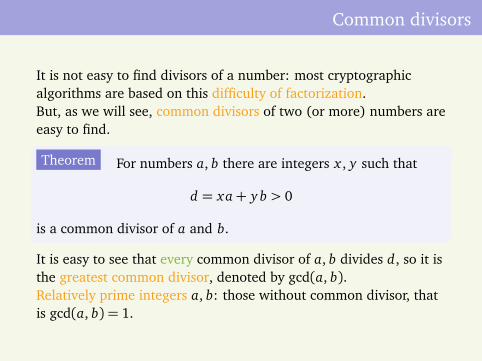
It is not easy to find divisors of a number: most cryptographicalgorithms are based on this difficulty of factorization.But, as we will see, common divisors of two (or more) numbers areeasy to find.

Theorem For numbers a, b there are integers x , y such that

d = xa+ y b > 0

is a common divisor of a and b.

It is easy to see that every common divisor of a, b divides d, so it isthe greatest common divisor, denoted by gcd(a, b).Relatively prime integers a, b: those without common divisor, thatis gcd(a, b) = 1.

Fundamental theorem

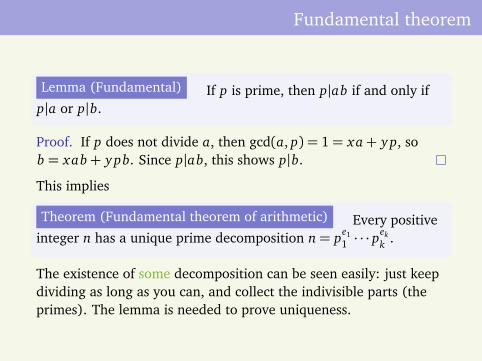
Lemma (Fundamental) If p is prime, then p|ab if and only ifp|a or p|b.

Proof. If p does not divide a, then gcd(a, p) = 1= xa+ yp, sob = xab+ ypb. Since p|ab, this shows p|b.

This implies

Theorem (Fundamental theorem of arithmetic) Every positiveinteger n has a unique prime decomposition n= pe1

1 · · · pekk .

The existence of some decomposition can be seen easily: just keepdividing as long as you can, and collect the indivisible parts (theprimes). The lemma is needed to prove uniqueness.

Euclid’s algorithm

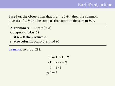
Based on the observation that if a = qb+ r then the commondivisors of a, b are the same as the common divisors of b, r.

Algorithm 8.1: EUCLID(a, b)Computes gcd(a, b)

1 if b = 0 then return a2 else return EUCLID(b, a mod b)

Example: gcd(30,21).

30= 1 · 21+ 9

21= 2 · 9+ 3

9= 3 · 3gcd= 3

Running time

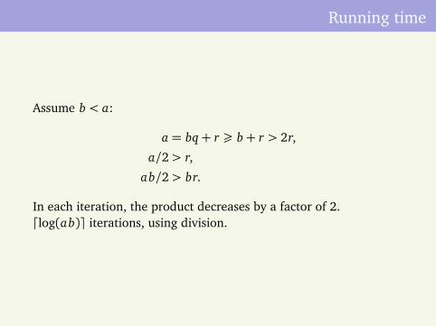
Assume b < a:

a = bq+ r ¾ b+ r > 2r,

a/2> r,

ab/2> br.

In each iteration, the product decreases by a factor of 2.dlog(ab)e iterations, using division.

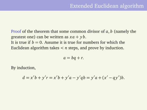
Extended Euclidean algorithm

Proof of the theorem that some common divisor of a, b (namely thegreatest one) can be written as xa+ y b.It is true if b = 0. Assume it is true for numbers for which theEuclidean algorithm takes < n steps, and prove by induction.

a = bq+ r.

By induction,

d = x ′b+ y ′r = x ′b+ y ′a− y ′qb = y ′a+ (x ′− q y ′)b.

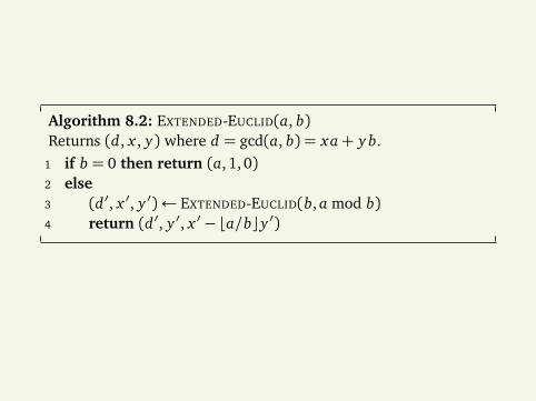
Algorithm 8.2: EXTENDED-EUCLID(a, b)Returns (d, x , y) where d = gcd(a, b) = xa+ y b.

1 if b = 0 then return (a, 1, 0)2 else3 (d ′, x ′, y ′)← EXTENDED-EUCLID(b, a mod b)4 return (d ′, y ′, x ′− ba/bcy ′)

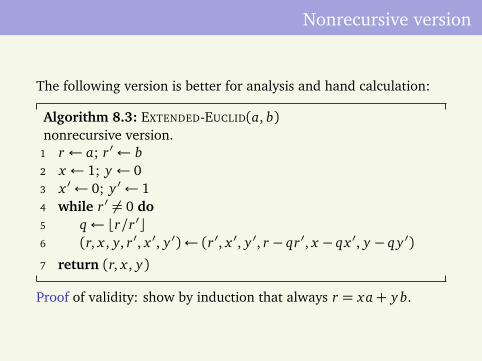
Nonrecursive version

The following version is better for analysis and hand calculation:

Algorithm 8.3: EXTENDED-EUCLID(a, b)nonrecursive version.

1 r ← a; r ′← b2 x ← 1; y ← 03 x ′← 0; y ′← 14 while r ′ 6= 0 do5 q← br/r ′c6 (r, x , y, r ′, x ′, y ′)← (r ′, x ′, y ′, r − qr ′, x − qx ′, y − q y ′)7 return (r, x , y)

Proof of validity: show by induction that always r = xa+ y b.

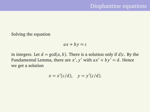
Diophantine equations

Solving the equation

ax + b y = c

in integers. Let d = gcd(a, b). There is a solution only if d|c. By theFundamental Lemma, there are x ′, y ′ with ax ′+ b y ′ = d. Hencewe get a solution

x = x ′(c/d), y = y ′(c/d).

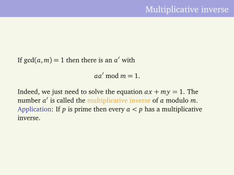
Multiplicative inverse

If gcd(a, m) = 1 then there is an a′ with

aa′ mod m= 1.

Indeed, we just need to solve the equation ax +my = 1. Thenumber a′ is called the multiplicative inverse of a modulo m.Application: If p is prime then every a < p has a multiplicativeinverse.

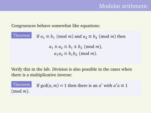
Modular arithmetic

Congruences behave somewhat like equations:

Theorem If a1 ≡ b1 (mod m) and a2 ≡ b2 (mod m) then

a1± a2 ≡ b1± b2 (mod m),

a1a2 ≡ b1 b2 (mod m).

Verify this in the lab. Division is also possible in the cases whenthere is a multiplicative inverse:

Theorem If gcd(a, m) = 1 then there is an a′ with a′a ≡ 1(mod m).

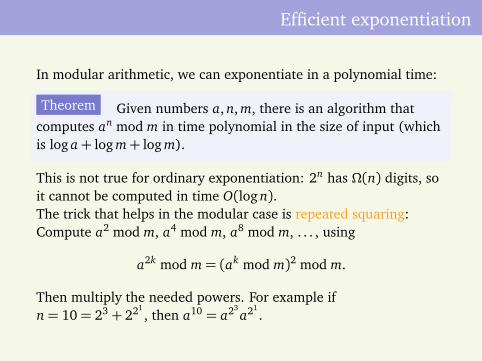
Efficient exponentiation

In modular arithmetic, we can exponentiate in a polynomial time:

Theorem Given numbers a, n, m, there is an algorithm thatcomputes an mod m in time polynomial in the size of input (whichis log a+ log m+ log m).

This is not true for ordinary exponentiation: 2n has Ω(n) digits, soit cannot be computed in time O(log n).The trick that helps in the modular case is repeated squaring:Compute a2 mod m, a4 mod m, a8 mod m, . . . , using

a2k mod m= (ak mod m)2 mod m.

Then multiply the needed powers. For example ifn= 10= 23+ 221

, then a10 = a23a21

.

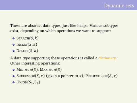
Dynamic sets

These are abstract data types, just like heaps. Various subtypesexist, depending on which operations we want to support:

SEARCH(S, k)

INSERT(S, k)

DELETE(S, k)

A data type supporting these operations is called a dictionary.Other interesting operations:

MINIMUM(S), MAXIMUM(S)

SUCCESSOR(S, x) (given a pointer to x), PREDECESSOR(S, x)

UNION(S1, S2)

Elementary data structures

You have studied these in the Data Structures course.Stack operations:

STACK-EMPTY(S)

PUSH(S, x)

POP(S)

Implement by array or linked list.Queue operations:

ENQUEUE(Q, x)

DEQUEUE(S, x)

Implement by circular array or linked list (with link to end).

Linked lists

Singly linked, doubly linked, circular.

LIST-SEARCH(L, k)

LIST-INSERT(L, x) (x is a record)

LIST-DELETE(L, x)

In the implementation, sentinel element nil[L] between the headand the tail to simplify boundary tests in a code.

Dynamic storage allocation

This underlies to a lot of data structure implementation.You must either explicitly implement freeing unused objects ofvarious sizes and returning the memory space used by them to freelists of objects of various sizes, or use some kind of garbagecollection algorithm.The present course just assumes that you have seen (or will see)some implementations in a Data Structures course (or elsewhere).

Representing trees

Binary tree data type, at least the following functions:

PARENT[x], LEFT[x], RIGHT[x].

We can represent all three functions explicitly by pointers.

Rooted trees with unbounded branching: One possiblerepresentation via a binary tree is the left-child, right-siblingrepresentation.

Other representations : Heaps, only parent pointers, and so on.

Hash tables

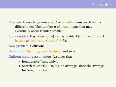
Problem A very large universe U of possible items, each with adifferent key. The number n of actual items that mayeventually occur is much smaller.

Solution idea Hash function h(k), hash table T[0 . . m− 1]. Key khashes to hash value (bucket) h(k).

New problem Collisions.

Resolution Chaining, open hashing, and so on.

Uniform hashing assumption Assumes thatItems arrive “randomly”.Search takes Θ(1+ n/m), on average, since the averagelist length is n/m.

Hash functions

What do we need? The hash function should spread the (hopefullyrandomly incoming) elements of the universe as uniformly aspossible over the table, to minimize the chance of collisions.

Keys into natural numbers It is easier to work with numbers thanwith words, so we translate words into numbers.For example, as radix 128 integers, possibly adding up theseintegers for different segments of the word.

Randomization: universal hashing

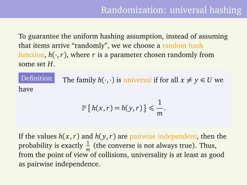
To guarantee the uniform hashing assumption, instead of assumingthat items arrive “randomly”, we we choose a random hashfunction, h(·, r), where r is a parameter chosen randomly fromsome set H.

Definition The family h(·, ·) is universal if for all x 6= y ∈ U wehave

P

h(x , r) = h(y, r)

¶1

m.

If the values h(x , r) and h(y, r) are pairwise independent, then theprobability is exactly 1

m(the converse is not always true). Thus,

from the point of view of collisions, universality is at least as goodas pairwise independence.

An example universal hash function

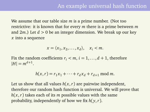
We assume that our table size m is a prime number. (Not toorestrictive: it is known that for every m there is a prime between mand 2m.) Let d > 0 be an integer dimension. We break up our keyx into a sequence

x = ⟨x1, x2, . . . , xd⟩, x i < m.

Fix the random coefficients ri < m, i = 1, . . . , d + 1, therefore|H|= md+1.

h(x , r) = r1 x1+ · · ·+ rd xd + rd+1 mod m.

Let us show that all values h(x , r) are pairwise independent,therefore our random hash function is universal. We will prove thath(x , r) takes each of its m possible values with the sameprobability, independently of how we fix h(y, r).

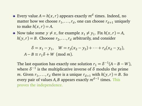
Every value A= h(x , r) appears exactly md times. Indeed, nomatter how we choose r1, . . . , rd , one can choose rd+1 uniquelyto make h(x , r) = A.

Now take some y 6= x , for example x1 6= y1. Fix h(x , r) = A,h(y, r) = B. Chooose r2, . . . , rd arbitrarily, and consider

δ = x1− y1, W = r2(x2− y2) + · · ·+ rd(xd − yd),

A− B ≡ r1δ+W (mod m).

The last equation has exactly one solution r1 = δ−1(A− B−W ),where δ−1 is the multiplicative inverse of δ modulo the primem. Given r1, . . . , rd there is a unique rd+1 with h(y, r) = B. Soevery pair of values A, B appears exactly md−1 times. Thisproves the independence.

Optional: perfect hashing

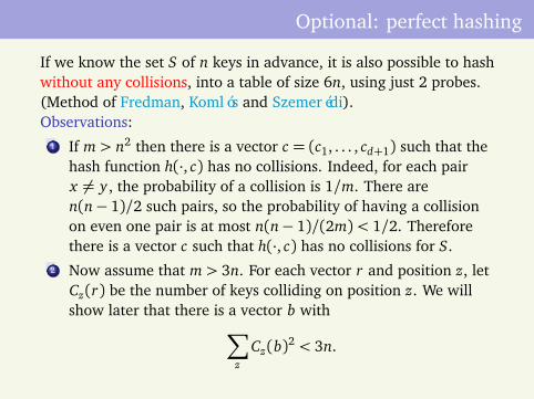
If we know the set S of n keys in advance, it is also possible to hashwithout any collisions, into a table of size 6n, using just 2 probes.(Method of Fredman, Komlós and Szemerédi).Observations:

1 If m> n2 then there is a vector c = (c1, . . . , cd+1) such that thehash function h(·, c) has no collisions. Indeed, for each pairx 6= y , the probability of a collision is 1/m. There aren(n− 1)/2 such pairs, so the probability of having a collisionon even one pair is at most n(n− 1)/(2m)< 1/2. Thereforethere is a vector c such that h(·, c) has no collisions for S.

2 Now assume that m> 3n. For each vector r and position z, letCz(r) be the number of keys colliding on position z. We willshow later that there is a vector b with

∑

zCz(b)

2 < 3n.

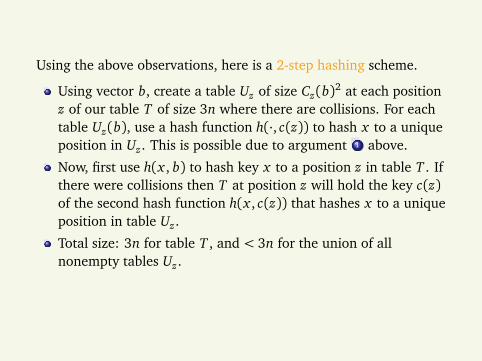
Using the above observations, here is a 2-step hashing scheme.

Using vector b, create a table Uz of size Cz(b)2 at each positionz of our table T of size 3n where there are collisions. For eachtable Uz(b), use a hash function h(·, c(z)) to hash x to a uniqueposition in Uz . This is possible due to argument 1 above.

Now, first use h(x , b) to hash key x to a position z in table T . Ifthere were collisions then T at position z will hold the key c(z)of the second hash function h(x , c(z)) that hashes x to a uniqueposition in table Uz .

Total size: 3n for table T , and < 3n for the union of allnonempty tables Uz .

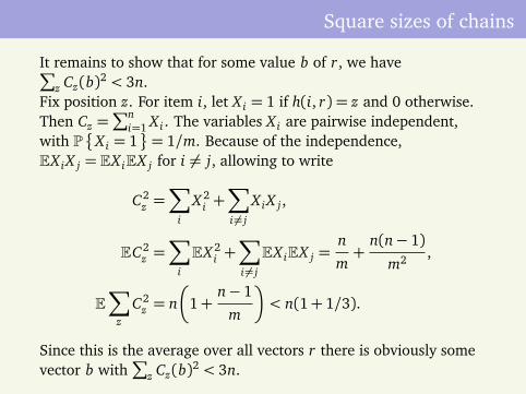
Square sizes of chains

It remains to show that for some value b of r, we have∑

z Cz(b)2 < 3n.Fix position z. For item i, let X i = 1 if h(i, r) = z and 0 otherwise.Then Cz =

∑ni=1 X i . The variables X i are pairwise independent,

with P

X i = 1

= 1/m. Because of the independence,EX iX j = EX iEX j for i 6= j, allowing to write

C2z =

∑

i

X 2i +∑

i 6= j

X iX j ,

EC2z =

∑

i

EX 2i +∑

i 6= j

EX iEX j =n

m+

n(n− 1)m2 ,

E∑

zC2

z = n

1+n− 1

m

< n(1+ 1/3).

Since this is the average over all vectors r there is obviously somevector b with

∑

z Cz(b)2 < 3n.

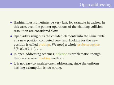
Open addressing

Hashing must sometimes be very fast, for example in caches. Inthis case, even the pointer operations of the chaining collisionresolution are considered slow.

Open addressing puts the collided elements into the same table,at a new position computed very fast. Looking for the newposition is called probing. We need a whole probe sequenceh(k, 0), h(k, 1, ), . . . .

In open addressing schemes, deletion is problematic, thoughthere are several marking methods.

It is not easy to analyze open addressing, since the uniformhashing assumption is too strong.

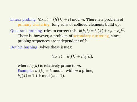
Linear probing h(k, i) = (h′(k) + i)mod m. There is a problem ofprimary clustering: long runs of collided elements build up.

Quadratic probing tries to correct this: h(k, i) = h′(k) + c1i+ c2i2.There is, however, a problem of secondary clustering, sinceprobing sequences are independent of k.

Double hashing solves these issues:

h(k, i) = h1(k) + ih2(k),

where h2(k) is relatively prime to m.Example: h1(k) = k mod m with m a prime,h2(k) = 1+ k mod (m− 1).

Search trees

Ordered left-to-right, items placed into the tree nodes (not onlyin leaves).

Inorder tree walk.

Search, min, max, successor, predecessor, insert, delete. All inO(h) steps.

Searches

Iterative or recursive TREE-SEARCH(x , k), where x is (a pointerto) the root.

Minimum and maximum are easy.

TREE-SUCCESSOR(x)

if right subtree of x is nonempty then its minimum.

else go up: return the first node to whom you had to stepright-up (if it exists).

Binary search treeInsertion and deletion

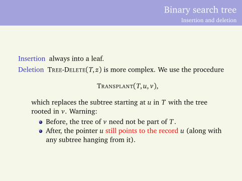
Insertion always into a leaf.

Deletion TREE-DELETE(T, z) is more complex. We use the procedure

TRANSPLANT(T, u, v),

which replaces the subtree starting at u in T with the treerooted in v. Warning:

Before, the tree of v need not be part of T .After, the pointer u still points to the record u (along withany subtree hanging from it).

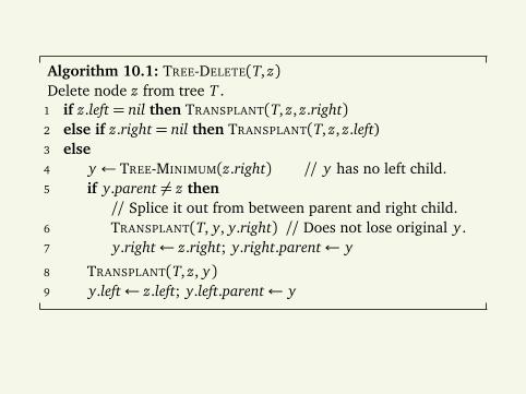
Algorithm 10.1: TREE-DELETE(T, z)Delete node z from tree T .

1 if z.left= nil then TRANSPLANT(T, z, z.right)2 else if z.right= nil then TRANSPLANT(T, z, z.left)3 else4 y ← TREE-MINIMUM(z.right) // y has no left child.5 if y.parent 6= z then

// Splice it out from between parent and right child.6 TRANSPLANT(T, y, y.right) // Does not lose original y .7 y.right← z.right; y.right.parent← y

8 TRANSPLANT(T, z, y)9 y.left← z.left; y.left.parent← y

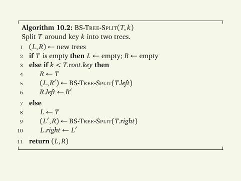
Algorithm 10.2: BS-TREE-SPLIT(T, k)Split T around key k into two trees.

1 (L, R)← new trees2 if T is empty then L← empty; R← empty3 else if k < T.root.key then4 R← T5 (L, R′)← BS-TREE-SPLIT(T.left)6 R.left← R′

7 else8 L← T9 (L′, R)← BS-TREE-SPLIT(T.right)

10 L.right← L′

11 return (L, R)

Randomized binary search trees

It can be shown (see book) that if n keys are inserted into abinary search tree in random order, then the expected height ofthe tree is only O(log n).

You cannot expect that keys will be inserted in random order.But it is possible (Martínez-Roura) to randomize the insertionand deletion operations in a way that will still guarantee thesame result.

Here is the idea of randomized insertion into a binary tree ofsize n.With probability 1

n+1, insert the key as root, and split the tree

around it.With probability 1− 1

n+1, randomized-insert recursively into the

left or right subtree, as needed.

There are corresponding deletion and join operations.

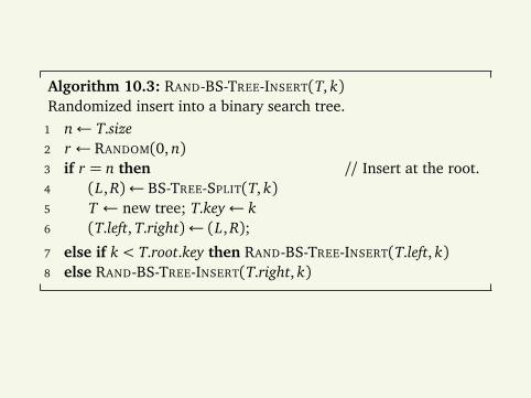
Algorithm 10.3: RAND-BS-TREE-INSERT(T, k)Randomized insert into a binary search tree.

1 n← T.size2 r ← RANDOM(0, n)3 if r = n then // Insert at the root.4 (L, R)← BS-TREE-SPLIT(T, k)5 T ← new tree; T.key← k6 (T.left, T.right)← (L, R);

7 else if k < T.root.key then RAND-BS-TREE-INSERT(T.left, k)8 else RAND-BS-TREE-INSERT(T.right, k)

Balanced trees

The cost of most common operations on search trees (search,insert, delete) is O(h), where h is the height.

We can claim h= O(log n) for the size n, if the tree is balanced.But keeping a tree completely balanced (say a binary tree ascomplete as possible) is as costly as maintaining a sorted array.

Idea: keep the tree only nearly balanced! The idea has severalimplementations: AVL trees, B-trees, red-black trees. We willonly see B-trees.

B-trees

Search trees, with the following properties, with a parameter t ¾ 2.

The records are kept in the tree nodes, sorted, “between” theedges going to the subtree.

Every path from root to leaf has the same length.

Every internal node has at least t − 1 and at most 2t − 1records (t to 2t children).

Total number of nodes n¾ 1+ t + · · ·+ th = th+1−1t−1

, showingh= O(logt n).

Maintaining a B-tree

Insertion Insert into the appropriate node. Split, if necessary. Ifthis requires split in the parent, too, split the parent.There is an implementation with only one, downward, pass. Itmakes sure that each subtree in which we insert, the root is notfull: has fewer than 2t − 1 keys. To achieve it, we splitproactively.

Deletion More complex, but also doable with one, downward,pass. Make sure that when we delete from a subtree, the roothas more than t − 1 (the minimum) keys. To achieve this,merge proactively.

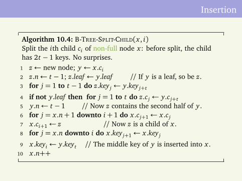
Insertion

Algorithm 10.4: B-TREE-SPLIT-CHILD(x , i)Split the ith child ci of non-full node x: before split, the childhas 2t − 1 keys. No surprises.

1 z← new node; y ← x .ci2 z.n← t − 1; z.leaf ← y.leaf // If y is a leaf, so be z.3 for j = 1 to t − 1 do z.key j ← y.key j+t

4 if not y.leaf then for j = 1 to t do z.c j ← y.c j+t5 y.n← t − 1 // Now z contains the second half of y .6 for j = x .n+ 1 downto i+ 1 do x .c j+1← x .c j7 x .ci+1← z // Now z is a child of x .8 for j = x .n downto i do x .key j+1← x .key j

9 x .keyi ← y.keyt // The middle key of y is inserted into x .10 x .n++

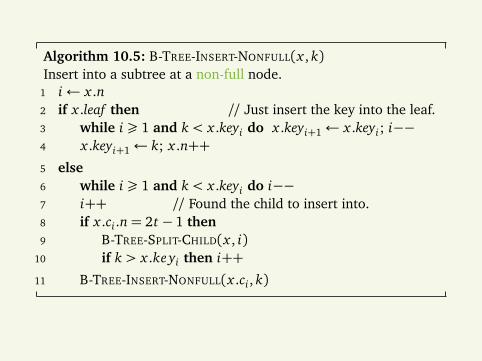
Algorithm 10.5: B-TREE-INSERT-NONFULL(x , k)Insert into a subtree at a non-full node.

1 i← x .n2 if x .leaf then // Just insert the key into the leaf.3 while i ¾ 1 and k < x .keyi do x .keyi+1← x .keyi; i−−4 x .keyi+1← k; x .n++

5 else6 while i ¾ 1 and k < x .keyi do i−−7 i++ // Found the child to insert into.8 if x .ci .n= 2t − 1 then9 B-TREE-SPLIT-CHILD(x , i)

10 if k > x .ke yi then i++

11 B-TREE-INSERT-NONFULL(x .ci , k)

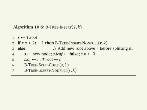
Algorithm 10.6: B-TREE-INSERT(T, k)

1 r ← T.root2 if r.n< 2t − 1 then B-TREE-INSERT-NONFULL(r, k)3 else // Add new root above r before splitting it.4 s← new node; s.leaf ← false; s.n← 05 s.c1← r; T.root← s6 B-TREE-SPLIT-CHILD(s, 1)7 B-TREE-INSERT-NONFULL(s, k)

Deletion

The deletion algorithm is more complex. See the book for anoutline, and try to implement it in pseudocode as an exercise.

Augmenting data structuresDynamic order statistics

Cache in each node the size of the subtree.

Retrieving an element with a given rank (selection).

Determining the rank of a given element.

Maintaining subtree sizes.

Dynamic programming

When there is a recursive algorithm based on subproblems but thetotal number of subproblems is not too great, it is possible to cache(memoize) all solutions in a table.

Fibonacci numbers.

Binomial coefficients.

(In both cases, the algorithm is by far not as good as computing theknown formulas.)

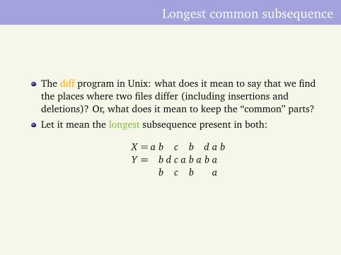
Longest common subsequence

The diff program in Unix: what does it mean to say that we findthe places where two files differ (including insertions anddeletions)? Or, what does it mean to keep the “common” parts?

Let it mean the longest subsequence present in both:

X = a b c b d a bY = b d c a b a b a

b c b a

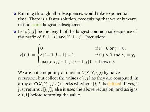
Running through all subsequences would take exponentialtime. There is a faster solution, recognizing that we only wantto find some longest subsequence.

Let c[i, j] be the length of the longest common subsequence ofthe prefix of X [1 . . i] and Y [1 . . j]. Recursion:

c[i, j] =

0 if i = 0 or j = 0,

c[i− 1, j− 1] + 1 if i, j > 0 and x i = y j ,

max(c[i, j− 1], c[i− 1, j]) otherwise.

We are not computing a function C(X , Y, i, j) by naiverecursion, but collect the values c[i, j] as they are computed, inarray c: C(X , Y, i, j, c) checks whether c[i, j] is defined. If yes, itjust returns c[i, j]; else it uses the above recursion, and assignsc[i, j] before returning the value.

Non-recursive implementation

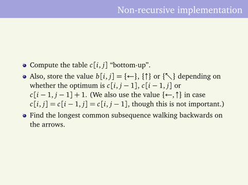
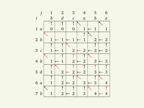
Compute the table c[i, j] “bottom-up”.

Also, store the value b[i, j] = ←, ↑ or depending onwhether the optimum is c[i, j− 1], c[i− 1, j] orc[i− 1, j− 1] + 1. (We also use the value ←,↑ in casec[i, j] = c[i− 1, j] = c[i, j− 1], though this is not important.)

Find the longest common subsequence walking backwards onthe arrows.

j 1 2 3 4 5 6i b d c a b a

↑ ↑ ↑ 1 a 0 0 0 1 ← 1 1 ↑

2 b 1 ← 1 ← 1 ← 1 2 ← 2↑ ↑ ↑ ↑

3 c 1 ← 1 2 ← 2 ← 2 ← 2 ↑ ↑ ↑

4 b 1 ← 1 2 ← 2 3 ← 3↑ ↑ ↑ ↑ ↑

5 d 1 2 ← 2 ← 2 3 ← 3↑ ↑ ↑ ↑

6 a 1 2 ← 2 3 ← 3 4 ↑ ↑ ↑ ↑

7 b 1 2 ← 2 3 4 ← 4

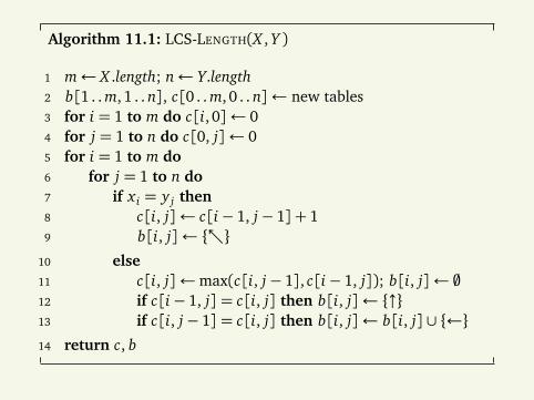
Algorithm 11.1: LCS-LENGTH(X , Y )

1 m← X .length; n← Y.length2 b[1 . . m, 1 . . n], c[0 . . m, 0 . . n]← new tables3 for i = 1 to m do c[i, 0]← 04 for j = 1 to n do c[0, j]← 05 for i = 1 to m do6 for j = 1 to n do7 if x i = y j then8 c[i, j]← c[i− 1, j− 1] + 19 b[i, j]←

10 else11 c[i, j]←max(c[i, j− 1], c[i− 1, j]); b[i, j]← ;12 if c[i− 1, j] = c[i, j] then b[i, j]← ↑13 if c[i, j− 1] = c[i, j] then b[i, j]← b[i, j]∪ ←14 return c, b

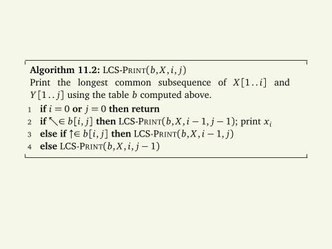
Algorithm 11.2: LCS-PRINT(b, X , i, j)Print the longest common subsequence of X [1 . . i] andY [1 . . j] using the table b computed above.

1 if i = 0 or j = 0 then return2 if∈ b[i, j] then LCS-PRINT(b, X , i− 1, j− 1); print x i3 else if ↑∈ b[i, j] then LCS-PRINT(b, X , i− 1, j)4 else LCS-PRINT(b, X , i, j− 1)

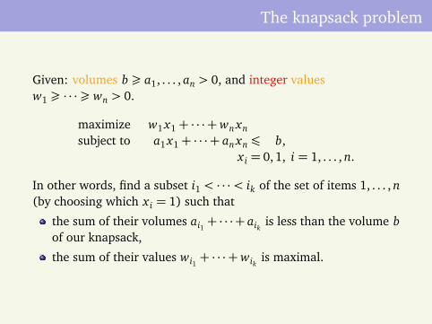
The knapsack problem

Given: volumes b ¾ a1, . . . , an > 0, and integer valuesw1 ¾ · · ·¾ wn > 0.

maximize w1 x1+ · · ·+wn xnsubject to a1 x1+ · · ·+ an xn ¶ b,

x i = 0,1, i = 1, . . . , n.

In other words, find a subset i1 < · · ·< ik of the set of items 1, . . . , n(by choosing which x i = 1) such that

the sum of their volumes ai1 + · · ·+ aik is less than the volume bof our knapsack,

the sum of their values wi1 + · · ·+wik is maximal.

Special cases

Subset sum problem find i1, . . . , ik with ai1 + · · ·+ aik = b.Obtained by setting wi = ai . Now if there is a solution withvalue b, we are done.

Partition problem Given numbers a1, . . . , an, find i1, . . . , ik suchthat ai1 + · · ·+ aik is as close as possible to (a1+ · · ·+ an)/2.

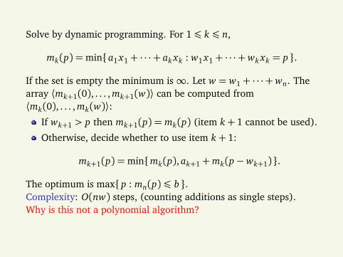
Solve by dynamic programming. For 1¶ k ¶ n,

mk(p) =min a1 x1+ · · ·+ ak xk : w1 x1+ · · ·+wk xk = p .

If the set is empty the minimum is∞. Let w = w1+ · · ·+wn. Thearray ⟨mk+1(0), . . . , mk+1(w)⟩ can be computed from⟨mk(0), . . . , mk(w)⟩:

If wk+1 > p then mk+1(p) = mk(p) (item k+ 1 cannot be used).

Otherwise, decide whether to use item k+ 1:

mk+1(p) =minmk(p), ak+1+mk(p−wk+1) .

The optimum is max p : mn(p)¶ b .Complexity: O(nw) steps, (counting additions as single steps).Why is this not a polynomial algorithm?

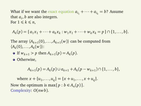
What if we want the exact equation ai1 + · · ·+ aik = b? Assumethat ai , b are also integers.For 1¶ k ¶ n,

Ak(p) = a1 x1+ · · ·+ ak xk : w1 x1+ · · ·+wk xk = p ∩ 1, . . . , b.

The array ⟨Ak+1(0), . . . , Ak+1(w)⟩ can be computed from⟨Ak(0), . . . , Ak(w)⟩:

If wk+1 > p then Ak+1(p) = Ak(p).

Otherwise,

Ak+1(p) = Ak(p)∪ ak+1+ Ak(p−wk+1)∩ 1, . . . , b,

where x + u1, . . . , uq= x + u1, . . . , x + uq.Now the optimum is max p : b ∈ An(p) .Complexity: O(nwb).

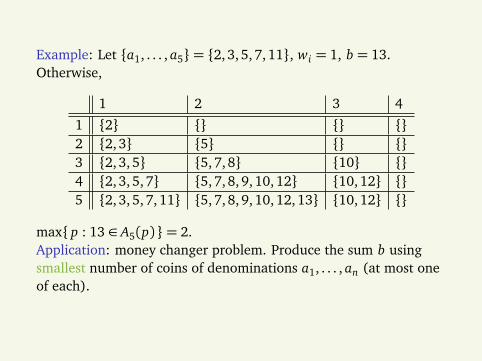
Example: Let a1, . . . , a5= 2,3, 5,7, 11, wi = 1, b = 13.Otherwise,

1 2 3 4

1 2 2 2,3 5 3 2,3, 5 5, 7,8 10 4 2,3, 5,7 5, 7,8, 9,10, 12 10, 12 5 2,3, 5,7, 11 5, 7,8, 9,10, 12,13 10, 12

max p : 13 ∈ A5(p) = 2.Application: money changer problem. Produce the sum b usingsmallest number of coins of denominations a1, . . . , an (at most oneof each).

Greedy algorithmsActivity selection

There is no general recipe. In general, greedy algorithms assumethat

There is an objective function f (x1, . . . , xn) to optimize thatdepends on some choices x1, . . . , xn. (Say, we need to maximizef ().)

There is a way to estimate, roughly, the contribution of eachchoice x i to the final value, but without taking into accounthow our choice will constrain the later choices.

The algorithm is greedy if it still makes the choice with the bestcontribution.

The greedy algorithm is frequently not the best, but sometimes it is.

Example: activity selection. Given: activities

[si , fi)

with starting time si and finishing time fi . Goal: to perform thelargest number of activites.Greedy algorithm: sort by fi . Repeatedly choose the activity withthe smallest fi compatible with the ones already chosen. Rationale:smallest fi restricts our later choices least.

Example

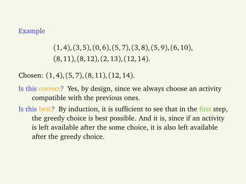
(1,4), (3,5), (0, 6), (5, 7), (3,8), (5,9), (6, 10),

(8,11), (8,12), (2, 13), (12,14).

Chosen: (1, 4), (5, 7), (8,11), (12,14).

Is this correct? Yes, by design, since we always choose an activitycompatible with the previous ones.

Is this best? By induction, it is sufficient to see that in the first step,the greedy choice is best possible. And it is, since if an activityis left available after the some choice, it is also left availableafter the greedy choice.

Knapsack

The knapsack problem, considered above under dynamicprogramming, also has a natural greedy algorithm. It is easy tosee that this is not optimal. (Exercise.)

But there is a version of this problem, called the fractionalknapsack problem, in which we are allowed to take any fractionof an item. The greedy algorithm is optimal in this case.(Exercise.)

Exhaustive searchMaximum independent set

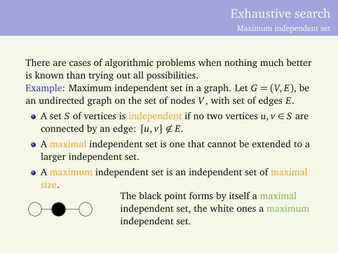
There are cases of algorithmic problems when nothing much betteris known than trying out all possibilities.Example: Maximum independent set in a graph. Let G = (V, E), bean undirected graph on the set of nodes V , with set of edges E.

A set S of vertices is independent if no two vertices u, v ∈ S areconnected by an edge: u, v 6∈ E.

A maximal independent set is one that cannot be extended to alarger independent set.

A maximum independent set is an independent set of maximalsize.

The black point forms by itself a maximalindependent set, the white ones a maximumindependent set.

It is easy to find a maximal independent set, but it is very hard tofind a maximum independent set. This is what we are interested in.Let NG(x) denote the set of neighbors of point x in graph G,including x itself.Let us fix a vertex x . There are two kinds of independent vertex setS: those that contain x , and and those that do not.

If x 6∈ S then S is an independent subset of the graph G \ x(of course, the edges adjacent to x are also removed from G).

If x ∈ S then S does not intersect NG(x), so S \ x is anindependent subset of G \ NG(x).

This gives rise to a simple recursive search algorithm.

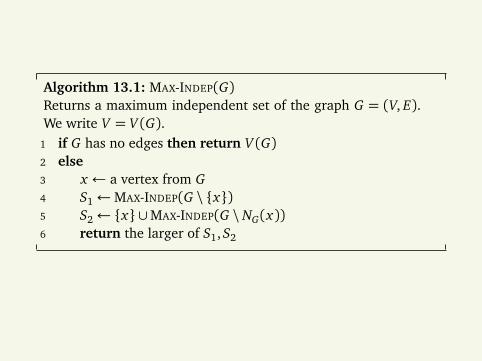
Algorithm 13.1: MAX-INDEP(G)Returns a maximum independent set of the graph G = (V, E).We write V = V (G).

1 if G has no edges then return V (G)2 else3 x ← a vertex from G4 S1←MAX-INDEP(G \ x)5 S2← x ∪MAX-INDEP(G \ NG(x))6 return the larger of S1, S2

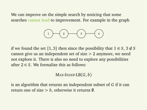
We can improve on the simple search by noticing that somesearches cannot lead to improvement. For example in the graph

2 3 41

if we found the set 1,3 then since the possibility that 1 ∈ S, 3 6∈ Scannot give us an independent set of size > 2 anymore, we neednot explore it. There is also no need to explore any possibilitiesafter 2 ∈ S. We formalize this as follows:

MAX-INDEP-LB(G, b)

is an algorithm that returns an independent subset of G if it canreturn one of size > b, otherwise it returns ;.

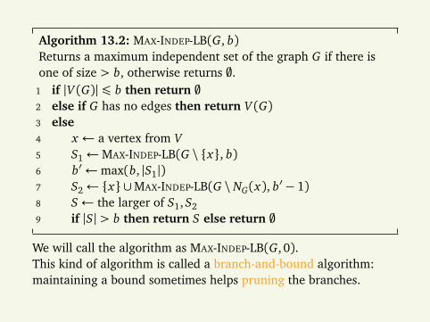
Algorithm 13.2: MAX-INDEP-LB(G, b)Returns a maximum independent set of the graph G if there isone of size > b, otherwise returns ;.

1 if |V (G)|¶ b then return ;2 else if G has no edges then return V (G)3 else4 x ← a vertex from V5 S1←MAX-INDEP-LB(G \ x, b)6 b′←max(b, |S1|)7 S2← x ∪MAX-INDEP-LB(G \ NG(x), b′− 1)8 S← the larger of S1, S29 if |S|> b then return S else return ;

We will call the algorithm as MAX-INDEP-LB(G, 0).This kind of algorithm is called a branch-and-bound algorithm:maintaining a bound sometimes helps pruning the branches.

Let us trace this algorithm on the graph

2 3 41

(6 1) : (G \ 1, 0)(6 1, 6 2) : (G \ 1,2, 0)(6 1, 6 2, 6 3) : (G \ 1,2, 3, 0) returns 4, b′ = 1(6 1, 6 2,3) : (G \ 1, 2,3,4, 1− 1= 0) returns ;,so (6 1, 6 2) : (G \ 1,2, 0) returns 4, b′ = 1.(6 1,2) : (G \ 1, 2,3, 1− 1= 0) returns 4,so (6 1) : (G \ 1, 0) returns 2, 4, b′ = 2.(1) : (G \ 1,2, 2− 1= 1)(1, 6 2, 6 3) : (G \ 1, 2,3, 1) returns ; by bound, b′ = 2.(1, 6 2, 3) : (G \ 1, 2,3, 4, 1− 1= 0) returns ;,so (1) : (G \ 1,2, 2− 1= 1) returns ; by bound,giving the final return 2, 4.

Graph representation

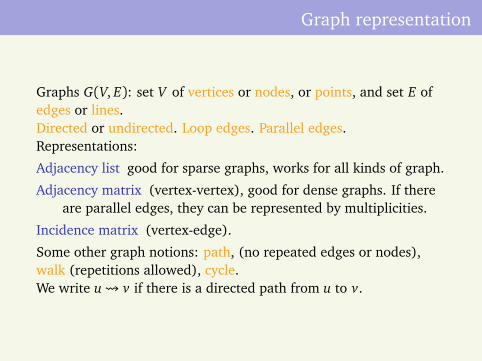
Graphs G(V, E): set V of vertices or nodes, or points, and set E ofedges or lines.Directed or undirected. Loop edges. Parallel edges.Representations:

Adjacency list good for sparse graphs, works for all kinds of graph.

Adjacency matrix (vertex-vertex), good for dense graphs. If thereare parallel edges, they can be represented by multiplicities.

Incidence matrix (vertex-edge).

Some other graph notions: path, (no repeated edges or nodes),walk (repetitions allowed), cycle.We write u v if there is a directed path from u to v.

Breadth-first search

Directed graph G = (V, E). Call some vertex s the source. Findsshortest path (by number of edges) from the source s to everyvertex reachable from s.Rough description of breadth-first search:

Distance x .d from s gets computed.

Black nodes have been visited.

Gray nodes frontier.

White nodes unvisited.

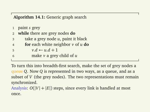
Algorithm 14.1: Generic graph search

1 paint s grey2 while there are grey nodes do3 take a grey node u, paint it black4 for each white neighbor v of u do5 v.d ← u.d + 16 make v a grey child of u

To turn this into breadth-first search, make the set of grey nodes aqueue Q. Now Q is represented in two ways, as a queue, and as asubset of V (the grey nodes). The two representations must remainsynchronized.Analysis: O(|V |+ |E|) steps, since every link is handled at mostonce.

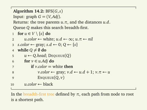
Algorithm 14.2: BFS(G, s)Input: graph G = (V, Adj).Returns: the tree parents u.π, and the distances u.d.Queue Q makes this search breadth-first.

1 for u ∈ V \ s do2 u.color← white; u.d ←∞; u.π← nil3 s.color← gray; s.d ← 0; Q← s4 while Q 6= ; do5 u←Q.head; DEQUEUE(Q)6 for v ∈ u.Adj do7 if v.color= white then8 v.color← gray; v.d ← u.d + 1; v.π← u9 ENQUEUE(Q, v)

10 u.color← black

In the breadth-first tree defined by π, each path from node to rootis a shortest path.

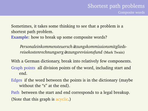
Shortest path problemsComposite words

Sometimes, it takes some thinking to see that a problem is ashortest path problem.Example: how to break up some composite words?

Personaleinkommensteuerschätzungskommissionsmitglieds-reisekostenrechnungsergänzungsrevisionsfund (Mark Twain)

With a German dictionary, break into relatively few components.

Graph points all division points of the word, including start andend.

Edges if the word between the points is in the dictionary (maybewithout the “s” at the end).

Path between the start and end corresponds to a legal breakup.

(Note that this graph is acyclic.)

The word breakup problem is an example where the graph isgiven only implicitly: To find out whether there is an edgebetween two points, you must make a dictionary lookup.

We may want to minimize those lookups, but minimizing twodifferent objective functions simultaneously (the number ofdivision points and the number of lookups) is generally notpossible.(For minimizing lookups, depth-first search seems better.)

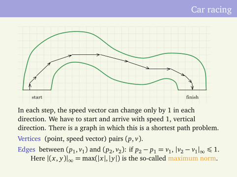
Car racing

start finish

In each step, the speed vector can change only by 1 in eachdirection. We have to start and arrive with speed 1, verticaldirection. There is a graph in which this is a shortest path problem.

Vertices (point, speed vector) pairs (p, v).

Edges between (p1, v1) and (p2, v2): if p2− p1 = v1, |v2− v1|∞ ¶ 1.Here |(x , y)|∞ =max(|x |, |y|) is the so-called maximum norm.

Depth-first search

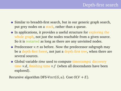
Similar to breadth-first search, but in our generic graph search,put grey nodes on a stack, rather than a queue.

In applications, it provides a useful structure for exploring thewhole graph, not just the nodes reachable from a given source.So it is restarted as long as there are any unvisited nodes.

Predecessor v.π as before. Now the predecessor subgraph maybe a depth-first forest, not just a depth-first tree, when there areseveral sources.

Global variable time used to compute timestamps: discoverytime v.d, finishing time v. f (when all descendants have beenexplored).

Recursive algorithm DFS-VISIT(G, u). Cost O(V + E).

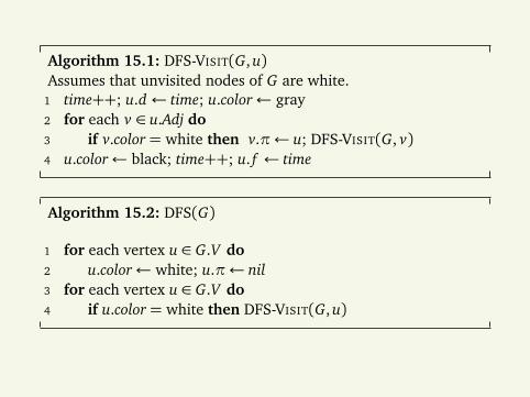
Algorithm 15.1: DFS-VISIT(G, u)Assumes that unvisited nodes of G are white.

1 time++; u.d ← time; u.color← gray2 for each v ∈ u.Adj do3 if v.color= white then v.π← u; DFS-VISIT(G, v)4 u.color← black; time++; u. f ← time

Algorithm 15.2: DFS(G)

1 for each vertex u ∈ G.V do2 u.color← white; u.π← nil3 for each vertex u ∈ G.V do4 if u.color= white then DFS-VISIT(G, u)

Properties of depth-first search

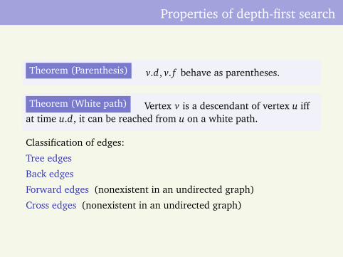
Theorem (Parenthesis) v.d, v. f behave as parentheses.

Theorem (White path) Vertex v is a descendant of vertex u iffat time u.d, it can be reached from u on a white path.

Classification of edges:

Tree edges

Back edges

Forward edges (nonexistent in an undirected graph)

Cross edges (nonexistent in an undirected graph)

Topological sort

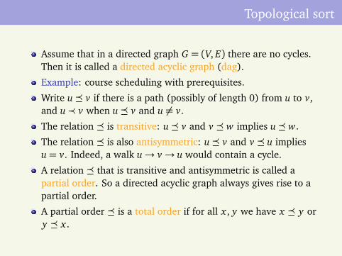
Assume that in a directed graph G = (V, E) there are no cycles.Then it is called a directed acyclic graph (dag).

Example: course scheduling with prerequisites.

Write u v if there is a path (possibly of length 0) from u to v,and u≺ v when u v and u 6= v.

The relation is transitive: u v and v w implies u w.

The relation is also antisymmetric: u v and v u impliesu= v. Indeed, a walk u→ v→ u would contain a cycle.

A relation that is transitive and antisymmetric is called apartial order. So a directed acyclic graph always gives rise to apartial order.

A partial order is a total order if for all x , y we have x y ory x .

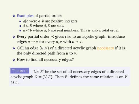
Examples of partial order:a|b were a, b are positive integers.A⊂ B where A, B are sets.a < b where a, b are real numbers. This is also a total order.

Every partial order ≺ gives rise to an acyclic graph: introduceedges u→ v for every u, v with u≺ v.

Call an edge (u, v) of a directed acyclic graph necessary if it isthe only directed path from u to v.

How to find all necessary edges?

Theorem Let E′ be the set of all necessary edges of a directedacyclic graph G = (V, E). Then E′ defines the same relation ≺ on Vas E.

Can we turn every partial order ≺ into a total order by addingsome more x ≺ y relations?

This is equivalent to the following: Given an acyclic graphG = (V, E), is there a listing v1, . . . , vn of its vertices in such away that if (vi , v j) ∈ E then i < j?

Yes, and DFS(G) finds the listing very efficiently. Sorting by v. f(backwards) is the desired order.

Theorem The graph G is acyclic iff DFS(G) yields no back edges.

Strongly connected components

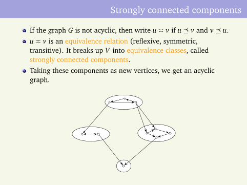
If the graph G is not acyclic, then write u v if u v and v u.

u v is an equivalence relation (reflexive, symmetric,transitive). It breaks up V into equivalence classes, calledstrongly connected components.

Taking these components as new vertices, we get an acyclicgraph.

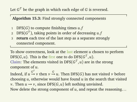
Let GT be the graph in which each edge of G is reversed.

Algorithm 15.3: Find strongly connected components

1 DFS(G) to compute finishing times u. f2 DFS(GT ), taking points in order of decreasing u. f3 return each tree of the last step as a separate strongly

connected component.

To show correctness, look at the last element u chosen to performDFS(G, u). This is the first one to do DFS(GT , u).Claim: The elements visited in DFS(GT , u) are in the strongcomponent of u.

Indeed, if uGT

v then vG u. Then DFS(G) has not visited v before

choosing u, otherwise would have found u in the search that visitedv. Then u v, since DFS(G, u) left nothing unvisited.Now delete the strong component of u, and repeat the reasoning. . .

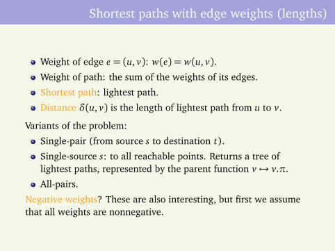
Shortest paths with edge weights (lengths)

Weight of edge e = (u, v): w(e) = w(u, v).

Weight of path: the sum of the weights of its edges.

Shortest path: lightest path.

Distance δ(u, v) is the length of lightest path from u to v.

Variants of the problem:

Single-pair (from source s to destination t).

Single-source s: to all reachable points. Returns a tree oflightest paths, represented by the parent function v 7→ v.π.

All-pairs.

Negative weights? These are also interesting, but first we assumethat all weights are nonnegative.

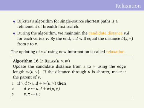
Relaxation

Dijkstra’s algorithm for single-source shortest paths is arefinement of breadth-first search.

During the algorithm, we maintain the candidate distance v.dfor each vertex v. By the end, v.d will equal the distance δ(s, v)from s to v.

The updating of v.d using new information is called relaxation.

Algorithm 16.1: RELAX(u, v, w)Update the candidate distance from s to v using the edgelength w(u, v). If the distance through u is shorter, make uthe parent of v.

1 if v.d > u.d +w(u, v) then2 d.v← u.d +w(u, v)3 v.π← u;

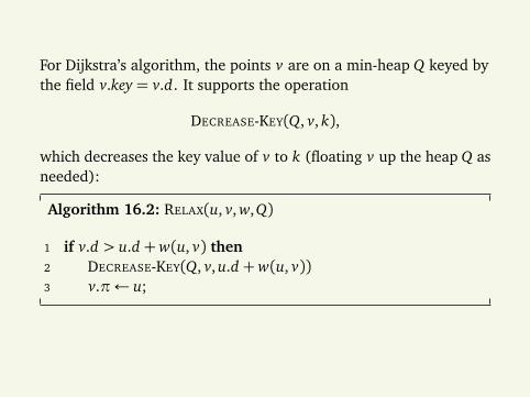
For Dijkstra’s algorithm, the points v are on a min-heap Q keyed bythe field v.key = v.d. It supports the operation

DECREASE-KEY(Q, v, k),

which decreases the key value of v to k (floating v up the heap Q asneeded):

Algorithm 16.2: RELAX(u, v, w,Q)

1 if v.d > u.d +w(u, v) then2 DECREASE-KEY(Q, v, u.d +w(u, v))3 v.π← u;

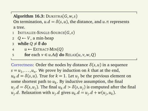
Algorithm 16.3: DIJKSTRA(G, w, s)On termination, u.d = δ(s, u), the distance, and u.π representsa tree.

1 INITIALIZE-SINGLE-SOURCE(G, s)2 Q← V , a min-heap3 while Q 6= ; do4 u← EXTRACT-MIN(Q)5 for each v ∈ u.Adj do RELAX(u, v, w,Q)

Correctness: Order the nodes by distance δ(s, u) in a sequences = u1, . . . , un. We prove by induction on k that at the end,uk.d = δ(s, u). True for k = 1. Let u j be the previous element onsome shortest path to uk. By inductive assumption, the finalu j .d = δ(s, u j). The final uk.d > δ(s, u j) is computed after the finalu j .d. Relaxation with u j .d gives uk.d = u j .d +w(u j , uk).

Cost of Dijkstra’s algorithm

Let n= |V |, m= |E|. Potentially a priority queue update for eachedge: O(m log n). This depends much on how dense is G.

All pairs, negative edges

Assume that there are no negative edge weights: To computedistances for all pairs, repeat Dijkstra’s algorithm from eachvertex as source. Complexity O(mn log n), not bad. But can beimproved, if G is dense, say m=Θ(n2).

If there are negative edges, new question: how about a negativecycle C? Then the minimum length of walks is −∞ (that is doesnot exist) between any pair of nodes u, v such that u C andC v. (A walk can go around a cycle any number of times.)

More modest goal: find out whether there is a negative cycle: ifthere is not, find all distances (shortest paths are then easy).

The Floyd-Warshall algorithm

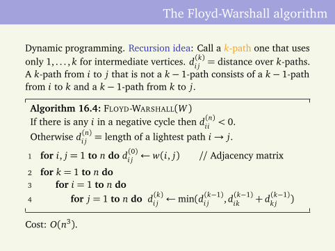
Dynamic programming. Recursion idea: Call a k-path one that usesonly 1, . . . , k for intermediate vertices. d(k)i j = distance over k-paths.A k-path from i to j that is not a k− 1-path consists of a k− 1-pathfrom i to k and a k− 1-path from k to j.

Algorithm 16.4: FLOYD-WARSHALL(W )If there is any i in a negative cycle then d(n)ii < 0.

Otherwise d(n)i j = length of a lightest path i→ j.

1 for i, j = 1 to n do d(0)i j ← w(i, j) // Adjacency matrix

2 for k = 1 to n do3 for i = 1 to n do4 for j = 1 to n do d(k)i j ←min(d(k−1)

i j , d(k−1)ik + d(k−1)

k j )

Cost: O(n3).

Applications

Transitive closure of a directed graph.

Arbitrage. Exchange rate x i j: this is how much it costs to buy aunit of currency j in currency i. Let w(i, j) =− log x i j . We canbecome infinitely rich if and only if there is negative cycle inthis graph.

Longest path in an acyclic graph

The Floyd-Warshall algorithm with negative weights would do it,but the following is more efficient.

1 for each vertex u in backwards topologically sorted order do2 for for each vertex v in u.Adj do RELAX(u, v, w)

(Of course, RELAX(u, v, w) is taking the maximum here, notminimum.)Application: finding the longest path is the basis of all projectplanning algorithms. (PERT method). You are given a number oftasks (for example courses with prerequisites). Figure out the leasttime needed to finish it all. This assumes unlimited resources, forexample ability to take any number of courses in a semester.

Minimum spanning trees

With respect to connectivity, another important algorithmicproblem is to find the smallest number of edges that still leaves anundirected graph connected. More generally, edges have weights,and we want the lightest tree. (Or heaviest, since negative weightsare also allowed.)Generic algorithm: add a safe edge each time: an edge that doesnot form a cycle with earlier selected edges.A cut of a graph G is any partition V = S ∪ T , S ∩ T = ;. It respectsedge set A if no edge of A crosses the cut. A light edge of a cut: alightest edge across it.

Theorem If A is a subset of some lightest spanning tree, S a cutrespecting A then after adding any light edge of S to A, theresulting A′ still belongs to some lightest spanning tree.

Prim’s algorithm

Keep adding a light edge adjacent to the already constructed tree.

Algorithm 17.1: MST-PRIM(G, w, r)Lightest spanning tree of (G, w), root r, returned in v.π.

1 for each vertex u do u.key←∞; u.π← nil2 r.key← 0; Q← G.V , a min-heap keyed by v.key3 while Q 6= ; do4 u← EXTRACT-MIN(Q)5 for v ∈ u.Adj do6 if v ∈Q and w(u, v)< v.key then v.π← u7 DECREASE-KEY(Q, v, w(u, v))

The only difference to Dijkstra’s algorithm is in how the key getsdecreased: it is set to the candidate lightest edge length from v tothe tree, not the candidate lightest path length from v to the root.

Matchings

Example (Workers and jobs) Suppose that we have n workersand n jobs. Each worker is capable of performing some of the jobs.Is it possible to assign each worker to a different job, so thatworkers get jobs they can perform?

It depends. If each worker is familiar only with the same one job(say, digging), then no.

Example At a dance party, with 300 students, every boy knows50 girls and every girl knows 50 boys. Can they all dancesimultaneously so that only pairs who know each other dance witheach other?

Bipartite graph: left set A (of girls), right set B (of boys).

Matching, perfect matching.

Theorem If every node of a bipartite graph has the same degreed ¾ 1 then it contains a perfect matching.

Examples showing the (local) necessity of the conditions:

Bipartiteness is necessary, even if all degrees are the same.

Bipartiteness and positive degrees is insufficient.

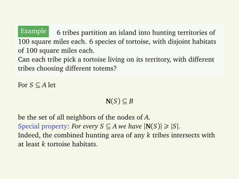
Example 6 tribes partition an island into hunting territories of100 square miles each. 6 species of tortoise, with disjoint habitatsof 100 square miles each.Can each tribe pick a tortoise living on its territory, with differenttribes choosing different totems?

For S ⊆ A let

N(S)⊆ B

be the set of all neighbors of the nodes of A.Special property: For every S ⊆ A we have |N(S)|¾ |S|.Indeed, the combined hunting area of any k tribes intersects withat least k tortoise habitats.

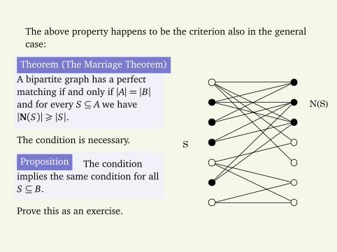
The above property happens to be the criterion also in the generalcase:

Theorem (The Marriage Theorem)

A bipartite graph has a perfectmatching if and only if |A|= |B|and for every S ⊆ A we have|N(S)|¾ |S|.

The condition is necessary.

Proposition The conditionimplies the same condition for allS ⊆ B.

Prove this as an exercise.

S

N(S)

Flow networks

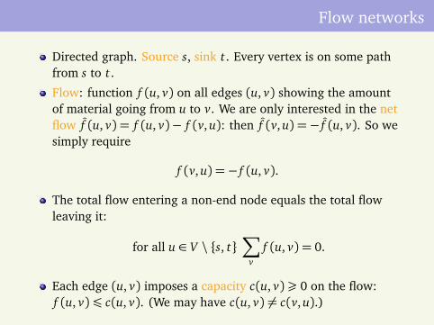
Directed graph. Source s, sink t. Every vertex is on some pathfrom s to t.

Flow: function f (u, v) on all edges (u, v) showing the amountof material going from u to v. We are only interested in the netflow f (u, v) = f (u, v)− f (v, u): then f (v, u) =− f (u, v). So wesimply require

f (v, u) =− f (u, v).

The total flow entering a non-end node equals the total flowleaving it:

for all u ∈ V \ s, t∑

vf (u, v) = 0.

Each edge (u, v) imposes a capacity c(u, v)¾ 0 on the flow:f (u, v)¶ c(u, v). (We may have c(u, v) 6= c(v, u).)

9/16

12/12

12/20

3/13

14

4

3/4 9 7s t

v1

v2

v3

v4

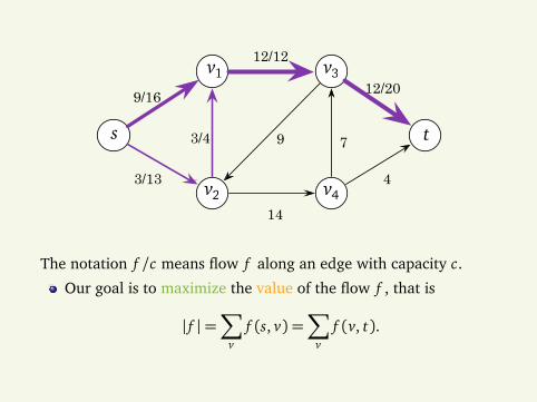
The notation f /c means flow f along an edge with capacity c.

Our goal is to maximize the value of the flow f , that is

| f |=∑

vf (s, v) =

∑

vf (v, t).

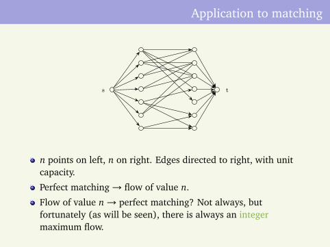
Application to matching

s t

n points on left, n on right. Edges directed to right, with unitcapacity.

Perfect matching→ flow of value n.

Flow of value n→ perfect matching? Not always, butfortunately (as will be seen), there is always an integermaximum flow.

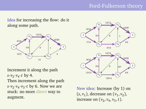
Ford-Fulkerson theory

Idea for increasing the flow: do italong some path.

9/16

12/12

12/20

3/13

14

4

3/4 9 7s t

v1

v2

v3

v4

Increment it along the paths-v2-v4-t by 4.Then increment along the paths-v2-v4-v3-t by 6. Now we arestuck: no more direct way toaugment.

9/16

12/12

12/20

7/13

4/14

4/4

3/4 9 7s t

v1

v2

v3

v4

9/16

12/12

18/20

13/13

10/14

4/4

3/4 9 6/7s t

v1

v2

v3

v4

New idea: Increase (by 1) on(s, v1), decrease on (v1, v2),increase on (v2, v4, v3, t).

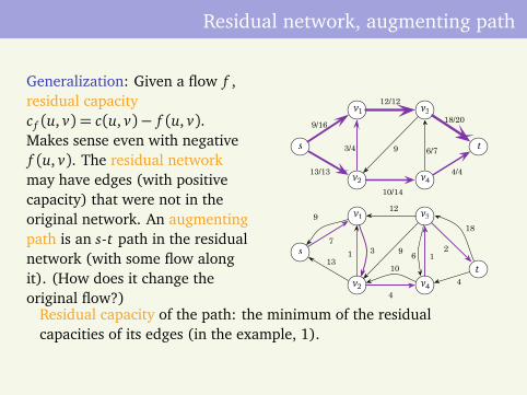
Residual network, augmenting path

Generalization: Given a flow f ,residual capacityc f (u, v) = c(u, v)− f (u, v).Makes sense even with negativef (u, v). The residual networkmay have edges (with positivecapacity) that were not in theoriginal network. An augmentingpath is an s-t path in the residualnetwork (with some flow alongit). (How does it change theoriginal flow?)

7

18

13

4

1 91s

t

v1

v2

v3

v4

9

3 2

4

10

9/16

12/12

18/20

13/13

10/14

4/4

3/4 9 6/7s t

v1

v2

v3

v4

12

6

Residual capacity of the path: the minimum of the residualcapacities of its edges (in the example, 1).

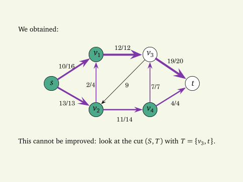
We obtained:

10/16

12/12

19/20

13/13

11/14

4/4

2/4 9 7/7s t

v1

v2

v3

v4

This cannot be improved: look at the cut (S, T ) with T = v3, t.

Method of augmenting paths

Keep increasing the flow along augmenting paths.Questions

1 If it terminates, did we reach maximum flow?2 Can we make it terminate?3 How many augmentations may be needed? Is this a

polynomial time algorithm?

Neither of these questions is trivial. The technique of cuts takescloser to the solution.

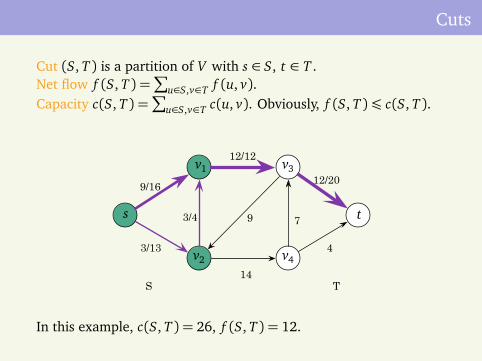
Cuts

Cut (S, T ) is a partition of V with s ∈ S, t ∈ T .Net flow f (S, T ) =

∑

u∈S,v∈T f (u, v).Capacity c(S, T ) =

∑

u∈S,v∈T c(u, v). Obviously, f (S, T )¶ c(S, T ).

9/16

12/12

12/20

3/13

14

4

3/4 9 7s t

v1

v2

v3

v4

S T

In this example, c(S, T ) = 26, f (S, T ) = 12.

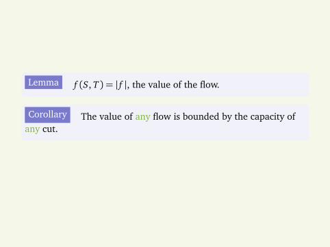
Lemma f (S, T ) = | f |, the value of the flow.

Corollary The value of any flow is bounded by the capacity ofany cut.

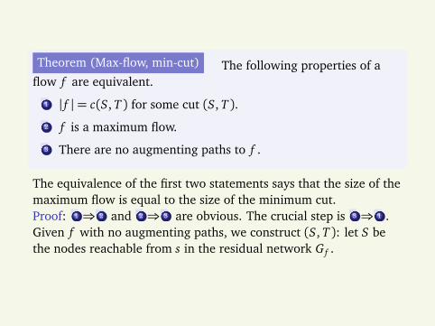
Theorem (Max-flow, min-cut) The following properties of aflow f are equivalent.

1 | f |= c(S, T ) for some cut (S, T ).

2 f is a maximum flow.

3 There are no augmenting paths to f .

The equivalence of the first two statements says that the size of themaximum flow is equal to the size of the minimum cut.Proof: 1 ⇒ 2 and 2 ⇒ 3 are obvious. The crucial step is 3 ⇒ 1 .Given f with no augmenting paths, we construct (S, T ): let S bethe nodes reachable from s in the residual network G f .

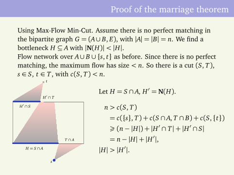
Proof of the marriage theorem

Using Max-Flow Min-Cut. Assume there is no perfect matching inthe bipartite graph G = (A∪ B, E), with |A|= |B|= n. We find abottleneck H ⊆ A with |N(H)|< |H|.Flow network over A∪ B ∪ s, t as before. Since there is no perfectmatching, the maximum flow has size < n. So there is a cut (S, T ),s ∈ S, t ∈ T , with c(S, T )< n.

H = S ∩ A

T ∩ A

H ∩ S

H ∩ T

s

t

Let H = S ∩ A, H ′ = N(H).

n> c(S, T )

= c(s, T ) + c(S ∩ A, T ∩ B) + c(S, t)¾ (n− |H|) + |H ′ ∩ T |+ |H ′ ∩ S|= n− |H|+ |H ′|,

|H|> |H ′|.

Polynomial-time algorithm

Does the Ford-Fulkerson algorithm terminate? Not necessarily(if capacities are not integers), unless we choose theaugmenting paths carefully.

Integer capacities: always terminates, but may takeexponentially long.Network derived from the bipartite matching problem: eachcapacity is 1, so we terminate in polynomial time.

Edmonds-Karp: use breadth-first search for the augmentingpaths. Why should this terminate?

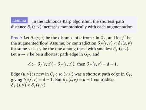
Lemma In the Edmonds-Karp algorithm, the shortest-pathdistance δ f (s, v) increases monotonically with each augmentation.

Proof: Let δ f (s, u) be the distance of u from s in G f , and let f ′ bethe augmented flow. Assume, by contradiction δ f ′(s, v)< δ f (s, v)for some v: let v be the one among these with smallest δ f ′(s, v).Let u→ v be be a shortest path edge in G f ′ , and

d := δ f (s, u)(= δ f ′(s, u)), then δ f ′(s, v) = d + 1.

Edge (u, v) is new in G f ′; so (v, u) was a shortest path edge in G f ,giving δ f (s, v) = d − 1. But δ f ′(s, v) = d + 1 contradictsδ f ′(s, v)< δ f (s, v).

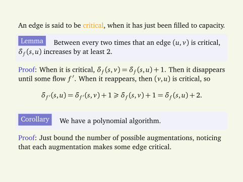
An edge is said to be critical, when it has just been filled to capacity.

Lemma Between every two times that an edge (u, v) is critical,δ f (s, u) increases by at least 2.

Proof: When it is critical, δ f (s, v) = δ f (s, u) + 1. Then it disappearsuntil some flow f ′. When it reappears, then (v, u) is critical, so

δ f ′(s, u) = δ f ′(s, v) + 1¾ δ f (s, v) + 1= δ f (s, u) + 2.

Corollary We have a polynomial algorithm.

Proof: Just bound the number of possible augmentations, noticingthat each augmentation makes some edge critical.

Let n= |V |, m= |E|. Each edge becomes critical at most n/2 times.Therefore there are at most m · n/2 augmentations. Eachaugmentation may take O(m) steps: total bound is

O(m2n).

There are better algorithms: Goldberg’s push-relabel algorithm,also given in your book, achieves O(n3).

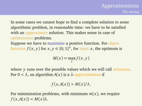
ApproximationsThe setting

In some cases we cannot hope to find a complete solution to somealgorithmic problem, in reasonable time: we have to be satisfiedwith an approximate solution. This makes sense in case ofoptimization problems.Suppose we have to maximize a positive function. For objectfunction f (x , y) for x , y ∈ 0,1n, for input x , the optimum is

M(x) =maxy

f (x , y)

where y runs over the possible values which we will call witnesses.For 0< λ, an algorithm A(x) is a λ-approximation if

f (x , A(x))> M(x)/λ.

For minimization problems, with minimum m(x), we requiref (x , A(x))< M(x)λ.

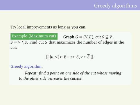
Greedy algorithms

Try local improvements as long as you can.

Example (Maximum cut) Graph G = (V, E), cut S ⊆ V ,S = V \ S. Find cut S that maximizes the number of edges in thecut:

| u, v ∈ E : u ∈ S, v ∈ S |.

Greedy algorithm:

Repeat: find a point on one side of the cut whose movingto the other side increases the cutsize.

Theorem If you cannot improve anymore with this algorithmthen you are within a factor 2 of the optimum.

Proof. The unimprovable cut contains at least half of all edges.

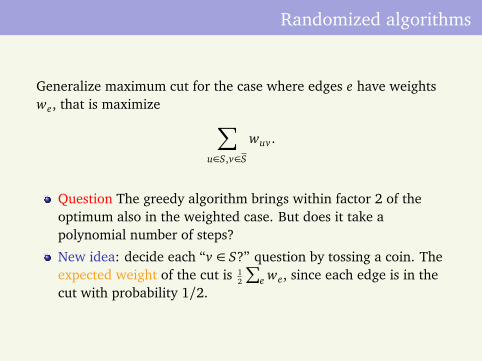
Randomized algorithms

Generalize maximum cut for the case where edges e have weightswe, that is maximize

∑

u∈S,v∈S

wuv .

Question The greedy algorithm brings within factor 2 of theoptimum also in the weighted case. But does it take apolynomial number of steps?

New idea: decide each “v ∈ S?” question by tossing a coin. Theexpected weight of the cut is 1

2

∑

e we, since each edge is in thecut with probability 1/2.

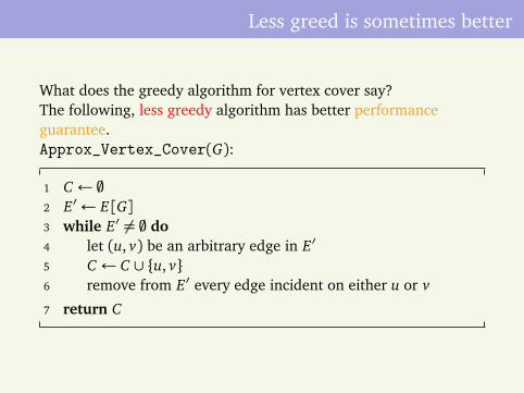
Less greed is sometimes better

What does the greedy algorithm for vertex cover say?The following, less greedy algorithm has better performanceguarantee.Approx_Vertex_Cover(G):

1 C ← ;2 E′← E[G]3 while E′ 6= ; do4 let (u, v) be an arbitrary edge in E′

5 C ← C ∪ u, v6 remove from E′ every edge incident on either u or v

7 return C

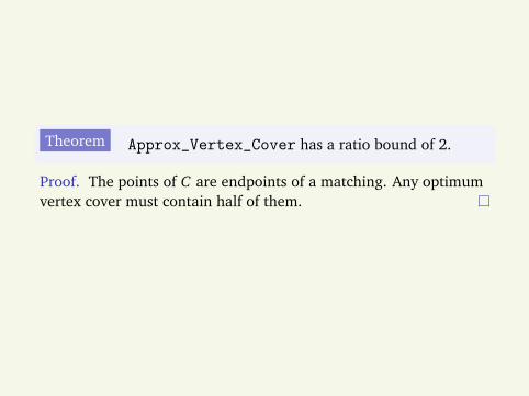
Theorem Approx_Vertex_Cover has a ratio bound of 2.

Proof. The points of C are endpoints of a matching. Any optimumvertex cover must contain half of them.

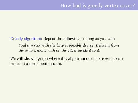
How bad is greedy vertex cover?

Greedy algorithm: Repeat the following, as long as you can:

Find a vertex with the largest possible degree. Delete it fromthe graph, along with all the edges incident to it.

We will show a graph where this algorithm does not even have aconstant approximation ratio.

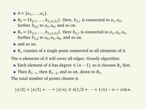
A= a1, . . . , an.B2 = b2,1, . . . , b2,bn/2c. Here, b2,1 is connected to a1, a2,further b2,2 to a3, a4, and so on.

B3 = b3,1, . . . , b3,bn/3c. Here b3,1 is connected to a1, a2, a3,further b3,2 to a4, a5, a6, and so on.

and so on.

Bn consists of a single point connected to all elements of A.

The n elements of A will cover all edges. Greedy algorithm:

Each element of A has degree ¶ (n− 1), so it chooses Bn first.

Then Bn−1, then Bn−2, and so on, down to B2.

The total number of points chosen is

bn/2c+ bn/3c+ · · ·+ bn/nc ¾ n(1/2+ · · ·+ 1/n)− n ∼ n ln n.

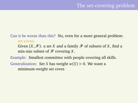
The set-covering problem

Can it be worse than this? No, even for a more general problem:set cover.Given (X ,F ): a set X and a family F of subsets of X , find amin-size subset of F covering X .

Example: Smallest committee with people covering all skills.

Generalization: Set S has weight w(S)> 0. We want aminimum-weight set cover.

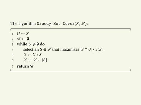
The algorithm Greedy_Set_Cover(X ,F ):

1 U ← X2 C ← ;3 while U 6= ; do4 select an S ∈ F that maximizes |S ∩ U |/w(S)5 U ← U \ S6 C ←C ∪ S7 return C

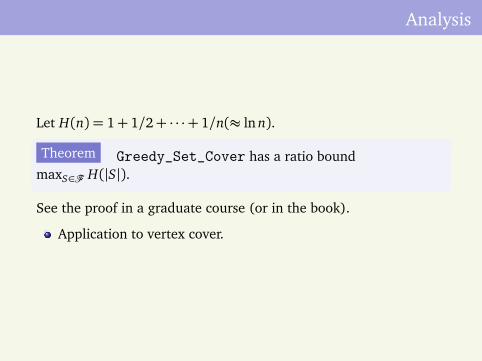
Analysis

Let H(n) = 1+ 1/2+ · · ·+ 1/n(≈ ln n).

Theorem Greedy_Set_Cover has a ratio boundmaxS∈F H(|S|).

See the proof in a graduate course (or in the book).

Application to vertex cover.

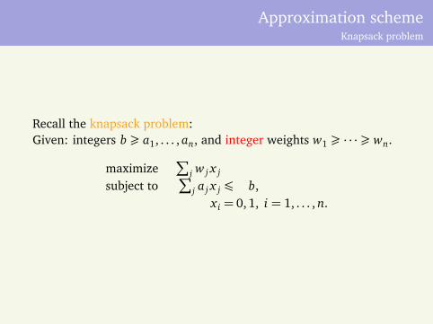
Approximation schemeKnapsack problem

Recall the knapsack problem:Given: integers b ¾ a1, . . . , an, and integer weights w1 ¾ · · ·¾ wn.

maximize∑

j w j x j

subject to∑

j a j x j ¶ b,x i = 0, 1, i = 1, . . . , n.

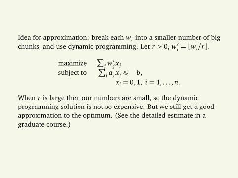
Idea for approximation: break each wi into a smaller number of bigchunks, and use dynamic programming. Let r > 0, w′i = bwi/rc.

maximize∑

j w′j x j

subject to∑

j a j x j ¶ b,x i = 0, 1, i = 1, . . . , n.

When r is large then our numbers are small, so the dynamicprogramming solution is not so expensive. But we still get a goodapproximation to the optimum. (See the detailed estimate in agraduate course.)

NP problems

Examples

shortest vs. longest simple paths

compositeness

subset sum

perfect matching

graph isomorphism

3-coloring

Ultrasound test of sex of fetus.

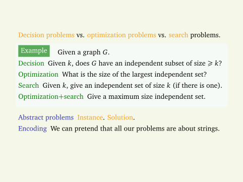
Decision problems vs. optimization problems vs. search problems.

Example Given a graph G.

Decision Given k, does G have an independent subset of size ¾ k?

Optimization What is the size of the largest independent set?

Search Given k, give an independent set of size k (if there is one).

Optimization+search Give a maximum size independent set.

Abstract problems Instance. Solution.

Encoding We can pretend that all our problems are about strings.

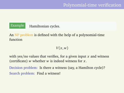
Polynomial-time verification

Example Hamiltonian cycles.

An NP problem is defined with the help of a polynomial-timefunction

V (x , w)

with yes/no values that verifies, for a given input x and witness(certificate) w whether w is indeed witness for x .

Decision problem: Is there a witness (say, a Hamilton cycle)?

Search problem: Find a witness!

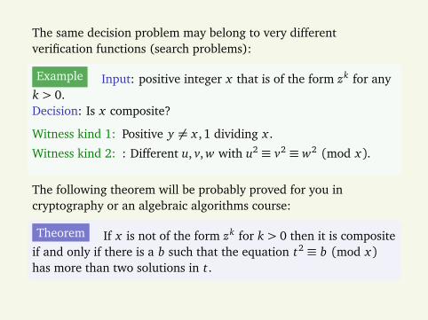
The same decision problem may belong to very differentverification functions (search problems):

Example Input: positive integer x that is of the form zk for anyk > 0.Decision: Is x composite?

Witness kind 1: Positive y 6= x , 1 dividing x .

Witness kind 2: : Different u, v, w with u2 ≡ v2 ≡ w2 (mod x).

The following theorem will be probably proved for you incryptography or an algebraic algorithms course:

Theorem If x is not of the form zk for k > 0 then it is compositeif and only if there is a b such that the equation t2 ≡ b (mod x)has more than two solutions in t.

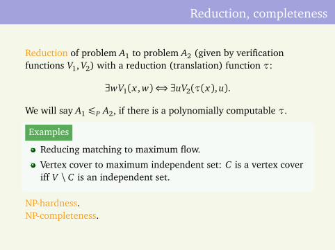
Reduction, completeness

Reduction of problem A1 to problem A2 (given by verificationfunctions V1, V2) with a reduction (translation) function τ:

∃wV1(x , w)⇔∃uV2(τ(x), u).

We will say A1 ¶P A2, if there is a polynomially computable τ.

Examples

Reducing matching to maximum flow.

Vertex cover to maximum independent set: C is a vertex coveriff V \ C is an independent set.

NP-hardness.NP-completeness.

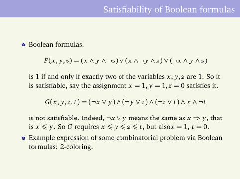
Satisfiability of Boolean formulas

Boolean formulas.

F(x , y, z) = (x ∧ y ∧¬z)∨ (x ∧¬y ∧ z)∨ (¬x ∧ y ∧ z)

is 1 if and only if exactly two of the variables x , y, z are 1. So itis satisfiable, say the assignment x = 1, y = 1, z = 0 satisfies it.

G(x , y, z, t) = (¬x ∨ y)∧ (¬y ∨ z)∧ (¬z ∨ t)∧ x ∧¬t

is not satisfiable. Indeed, ¬x ∨ y means the same as x ⇒ y , thatis x ¶ y . So G requires x ¶ y ¶ z ¶ t, but alsox = 1, t = 0.

Example expression of some combinatorial problem via Booleanformulas: 2-coloring.

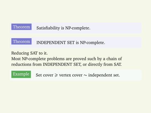
Theorem Satisfiability is NP-complete.

Theorem INDEPENDENT SET is NP-complete.

Reducing SAT to it.Most NP-complete problems are proved such by a chain ofreductions from INDEPENDENT SET, or directly from SAT.

Example Set cover ¾ vertex cover ∼ independent set.

The End