Algorithms for Memory HierarchiesLecture 3

Lecturer: Nodari SitchinavaScribes: Mateus Grellert, Robin Rehrmann

• Last time: B-trees

• Today: Persistent B-trees

1 Persistent B-trees

When it comes to (a,b)-trees, in general, and B-trees - which are (a,b)-trees with a = B4

and b = B (Figure 1) - specifically, one could wonder, what these trees are used for.

Figure 1: A B-tree.

One of the fields in which B-trees are commonly used are databases. Databases use B-trees to index data, because they provide an efficient way, to insert, search and updatedata.

1

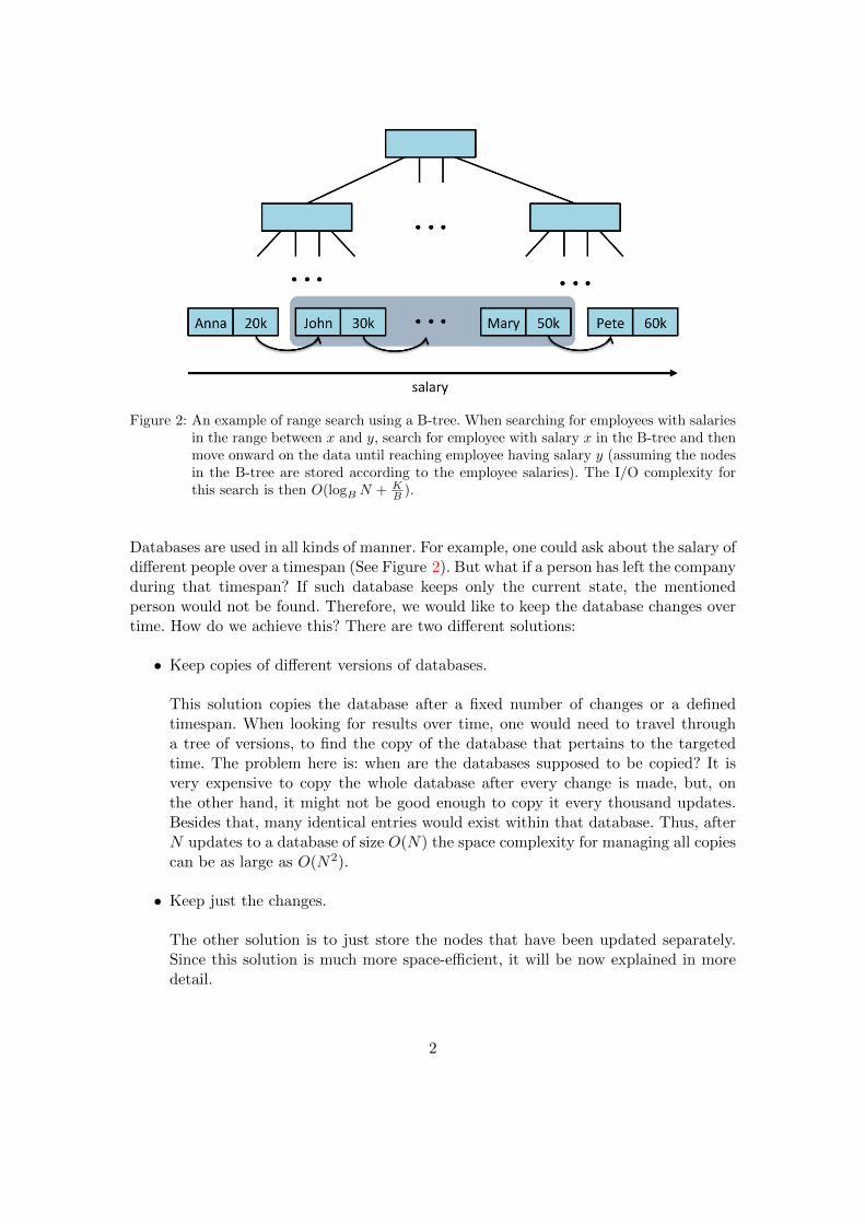
Figure 2: An example of range search using a B-tree. When searching for employees with salariesin the range between x and y, search for employee with salary x in the B-tree and thenmove onward on the data until reaching employee having salary y (assuming the nodesin the B-tree are stored according to the employee salaries). The I/O complexity forthis search is then O(logB N + K

B ).

Databases are used in all kinds of manner. For example, one could ask about the salary ofdifferent people over a timespan (See Figure 2). But what if a person has left the companyduring that timespan? If such database keeps only the current state, the mentionedperson would not be found. Therefore, we would like to keep the database changes overtime. How do we achieve this? There are two different solutions:

• Keep copies of different versions of databases.

This solution copies the database after a fixed number of changes or a definedtimespan. When looking for results over time, one would need to travel througha tree of versions, to find the copy of the database that pertains to the targetedtime. The problem here is: when are the databases supposed to be copied? It isvery expensive to copy the whole database after every change is made, but, onthe other hand, it might not be good enough to copy it every thousand updates.Besides that, many identical entries would exist within that database. Thus, afterN updates to a database of size O(N) the space complexity for managing all copiescan be as large as O(N2).

• Keep just the changes.

The other solution is to just store the nodes that have been updated separately.Since this solution is much more space-efficient, it will be now explained in moredetail.

2

1.1 Types of persistent data structure

There are two different types of persistent data structures, which differ from each otherwhen it comes to the possibility of updating and querying past versions of the datastructure.

Fully persistent data structures allow you to query and update any version in thepast. This is a quite complicated algorithm and most of the time not needed. What ismore important is the second type of persistent data structure.

Partially persistent data structures also allow you to query any version in the past,but only the most recent version can be updated. Since this is a simpler algorithm,and since it also provides anything one mostly needs, today we will talk about partiallypersistent B-trees.

1.2 Partially persistent B-trees

In order to control the different versions, each insertion and deletion operation on thetree is augmented with a timestamp of when it is performed, like shown on the tablebelow.

insert(x) insert(y) delete(y) insert(z) delete(x)

t 1 2 3 4 5

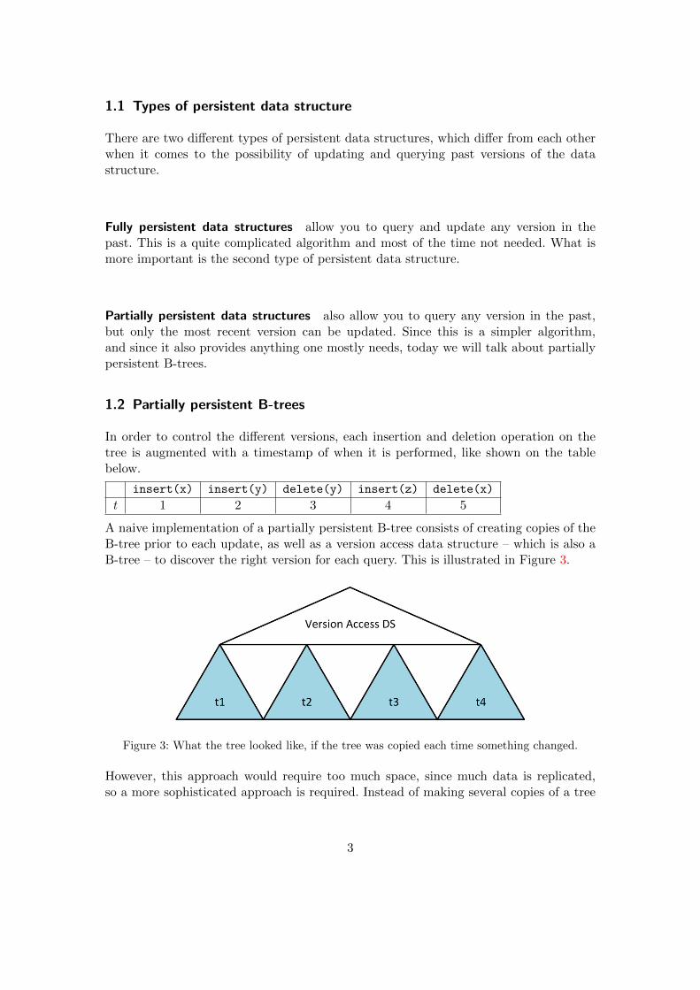
A naive implementation of a partially persistent B-tree consists of creating copies of theB-tree prior to each update, as well as a version access data structure – which is also aB-tree – to discover the right version for each query. This is illustrated in Figure 3.

Figure 3: What the tree looked like, if the tree was copied each time something changed.

However, this approach would require too much space, since much data is replicated,so a more sophisticated approach is required. Instead of making several copies of a tree

3

whenever an update occurs, only new information should alter the structure. In orderto do so, each node must contain its existence interval [ti, tj ]. E.g. the element x in thetable above was stored as x[1, 5]. The resulting structure is not a tree, but a DirectedAcyclic Graph (DAG), topped by a version control structure, which is, again, also aB-tree, as depicted in Figure 4.

Figure 4: The Direct Acyclic Graph (DAG) returning the root node of the selected timestampof the B-tree.

At any given time, the nodes that are alive constitute a valid B-tree, i.e., each nodecontains [B4 , B] living nodes. Each new node must follow the new node invariant, whichstates that a new node contains only elements that are alive.

1.2.1 The new node invariant

Now we introduce an invariant for new nodes. As previously mentioned, new nodes alwayscontain only alive elements. Additionally, whenever we create a new node we restrict thenumber of elements n in the new node to be 3

8B ≤ |n| ≤78B. In other words, the number

of elements is at least 38B, instead of 1

4B, and at most 78B, instead of B.

The new node invariants guarantee linear space of the persistent B-tree. But beforewe analyze the space and I/O complexity, let us first describe the operations on thepersistent B-tree.

1.3 Update operations in the Persistent B-trees

We will now describe how to perform insertion and deletion in the persistent B-tree.

1.3.1 Inserting an element into the persistent B-tree

When inserting an element into the B-tree, we first find the leaf in which the elementshould be placed at. Finding this leaf is done with the search method (see Program 1).

4

To do this, we first query the version access structure to the root that is valid at time t.Afterwards, within the returned tree we search for the leaf that will hold the element tobe inserted. Since we search in B-trees, the cost for this operation so far is 2·O(logB N) =O(logB N).

1 search(x, t)2 vas = get_version_access_structure ();

3 btree = vas.find_root_at_time(t);4 return btree.find(x);5

6 insert(x, t)7 l = search(x, t);8 l.insert(x);9

10 if( |l| > B )

11 l′ = copy_alive_elements(l); // 14B ≤ l′ ≤ B + 1

12 set_timestamp(l′, t);13 mark_as_deleted(l);14 update(parent(l), l, l′); // update pointers of parent node

15 rebalance(l′);16

17 rebalance(v) // 14B ≤ v ≤ B + 1

18 if( 38B ≤ |v| ≤

78B )

19 return;

20 if( |v| > 78B )

21 strong_overflow(v);

22 if( |v| < 38B )

23 strong_underflow(v);24

25 rebalance(parent(v));

Program 1: Implementations of the methods search and insert and helper method rebalance

After inserting element x into leaf l, that leaf may need to be rebalanced. This is done inProgram 2. Therefore l is marked as deleted inside of its parent and all its alive elementsare copied into a new leaf l′. This new leaf is sent to method rebalance, in which we firstneed to check whether the size of the new node (i.e. its number of elements) is between38B and 7

8B. If so, nothing happens.

Otherwise, if |v′| > 78B, the method strong_overflow is called, which splits the given

node into two nodes of the same size (±1, depending on, whether v is even, or not) andupdates the parent of v.

Instead, if |v′| < 38B, the method strong_underflow is called. This fuses the alive

elements of the sibling v′ of v and v into a single node v. Since that sibling had at least14B alive elements and the new node has 1

4B − 1 alive elements, the fused node now hasat least 1

2B − 1 elements and our invariant of having at least 38B elements is satisfied. If

5

the new node contains less than 78B elements, all that remains to do is update pointers

in the parent node and rebalance the parent node if needed. On the other hand, becausethe sibling may hold B elements, the new node might contain too many elements. If so,it again needs to be split up into two new nodes having equal number of elements (±1depending on the parity of B).

1 /* This method is called , if |v| > 78B. */

2 strong_overflow(v)

3 create v′, v′′ so that |v′| =⌊|v|2

⌋, |v′′| =

⌈|v|2

⌉≥ 3

8B

4 update(parent(v), v, v′, v′′); // update pointers of parent node

5

6 /* parent(v)’s size increased by 1, so recursively rebalance */

7 rebalance(parent(v));8

9 /* This method is called , if 14B ≤ |v| <

38B. */

10 strong_underflow(v)11 v′ = get_sibling(v);12

13 /* Create a copy of sibling without dead elements. */

14 v′′ = copy_alive_elements(v′); // |v′′| ≥ 14B

15 mark_as_dead(v′);16

17 /* Fuse v and v′′ */

18 v = fuse(v, v′′) // |v| ≥ 12B − 1

19

20 if( |v| < 78B )

21 update(parent(v), v, v′); // update pointers of parent node

22

23 /* parent(v)’s size decreased by 1, so recursively rebalance */

24 rebalance(parent(v));25 else

26 // |u|, |u′| ≥ 38B

27 u,u′ = split(v);28 update(parent(v), v, u, u′); // update pointers of parent node

Program 2: Implementations of the helper methods strong_overflow and strong_underflow.

1.3.2 Method delete for removing an element from the persistent B-tree

When deleting an element from the tree, we first search for the leaf holding that element(Program 3). Within that returned leaf the element to be deleted is marked as deleted,because, since we want to keep the old versions, we do not want to erase it completely.

Afterwards, it needs to be checked whether that node contains a valid number of aliveelements, i.e., the number of alive (meaning the elements that have not been marked asdeleted) must be at least 1

4B. If not so, a copy of l is created, that contains all the alive

6

1 delete(x, t)2 {

3 l = search(x);4 // do not delete x within l, just mark it as deleted.

5 l.mark_as_deleted(x);6

7 // now check for the number of active elements

8 if( |alive_elements(l)| ≤ 14B )

9 // Create a copy of l. The copy does not

10 // hold dead elements.

11 l′ = copy_alive_elements(l);12

13 // because |l′| < 38B

14 strong_underflow(l′);15

16 // mark as deleted in parent

17 update(parent(l));18 rebalance(parent(l), l, l′);19 }

Program 3: Implementations of delete. This function also uses helper functions, implementedin Program 2.

elements of l only. With this copy l′, we call the method strong_underflow, because l′

cannot hold 38B elements, since the original l contained less than 1

4B alive elements.

Afterwards, l needs to be marked as deleted inside of its parent, and the parent isrebalanced, if needed.

1.4 Analysis

Let us analyze the I/O-complexity of N operations on a persistent B-tree.

Search When searching an element after N operations, the I/O-complexity of thatsearch is O(logB N) I/Os. That is, because the search within the Version Access Datastructure is O(logB N) I/Os and the search within the returned B-tree is also O(logB N)I/Os, which leads to a total complexity of O(logB N) I/Os.

Insert/delete When inserting or deleting an element into or out of the tree, we firsthave to search this element (we now know that the complexity of the search is O(logB N)I/Os). When the node is found, the insert/delete operation takes O(1) I/Os in that node(since rebalancing touches at most two nodes of one block each per level). In the worstcase, every predecessor of such node, up to the root, need to be updated with the samenumber of constant I/Os, so, in the worst case, this takes O(1) ·O(logB N). So all in all

7

the complexity of inserting or deleting an element is O(logB N) + O(1) · O(logB N) =O(logB N).

Now let us have a look at the space required by the data structure. We will show thatthe space complexity for this scenario is O(NB ) blocks. And this is where our new nodeinvariants come in.

When doing an update, we do not free any memory. So how do we guarantee thateventually after many copies are performed the data structure does not take up toomuch space?

When a new node is created as a copy of an old node, it has at least 38B elements (by

the new node invariant), so it takes at least 18B deletes from this node to create a new

copy from it again. On the other hand, a new node has at most 78B elements, so it takes

at least 18B updates, to create a new copy from it, again. So all in all, it takes at least

18B operations on a new node, to create a new copy and ”waste” space, again.

So, after N operations, we have created less than N18B

copies of that node. Since a node

is only copied, when its children are updated, the parent of this node is copied less thanN

( 18B)2

times after N operations. Finally, when looking at the total amount of space on all

levels of the tree, the space complexity can be represented by the following equation:

logB N∑i=1

N

(18B)i= O

(N

B

)blocks

Therefore, the new node invariant is introduced in order to guarantee that not too muchspace is used, since linear space complexity is achieved by using this rule.

1.5 Persistent B-trees Applications

The problem of finding intersections in a set of orthogonal line segments can be modeledwith a Persistent B-tree. Each begin/end coordinate can be considered the same as thetimestamps ti and tj . Figure 5 is shown, to illustrate this.

Here, we query via SQL in past versions (as we have already seen). Having B-trees, theI/O complexity for this query is O(logB N + T

B ). So for N horizontal segments the totalcomplexity is O(N logB N + T

B ) I/Os.

In two lectures, though, we will see, how to get from O(N logB N + TB ) I/Os

to O(NB logMB

NB + T

B ) I/Os, which is a lot fewer I/Os, since N � sort(N) =

O(NB logMB

NB ).

8

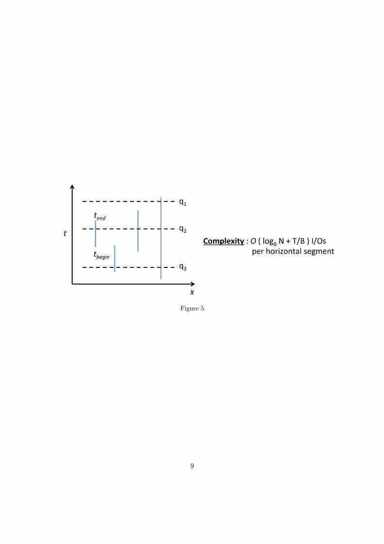
Figure 5

9