UNIVERSITY OF CALIFORNIA

Irvine

Algorithms and Heuristics

for Constraint Satisfaction Problems

A dissertation submitted in partial satisfaction of the

requirements for the degree Doctor of Philosophy

in Information and Computer Science

by

Daniel Hunter Frost

Committee in charge:

Professor Rina Dechter, Chair

Professor Dennis Kibler

Professor Richard H. Lathrop

1997

c 1997

DANIEL HUNTER FROST

ALL RIGHTS RESERVED

The dissertation of Daniel Hunter Frost is approved,

and is acceptable in quality and form for

publication on micro�lm:

Committee Chair

University of California, Irvine

1997

ii

To Kathy

iii

Contents

List of Figures : : : : : : : : : : : : : : : : : : : : : : : : : : : : : : : : vii

List of Tables : : : : : : : : : : : : : : : : : : : : : : : : : : : : : : : : : x

Acknowledgements : : : : : : : : : : : : : : : : : : : : : : : : : : : : : xi

Curriculum Vitae : : : : : : : : : : : : : : : : : : : : : : : : : : : : : : xii

Abstract : : : : : : : : : : : : : : : : : : : : : : : : : : : : : : : : : : : : xiii

Chapter 1 Introduction : : : : : : : : : : : : : : : : : : : : : : : : : 11.1 Introduction : : : : : : : : : : : : : : : : : : : : : : : : : : : : : : : 11.2 Background : : : : : : : : : : : : : : : : : : : : : : : : : : : : : : : 31.3 Methodology : : : : : : : : : : : : : : : : : : : : : : : : : : : : : : 81.4 Related Work : : : : : : : : : : : : : : : : : : : : : : : : : : : : : : 131.5 Overview of the Dissertation : : : : : : : : : : : : : : : : : : : : : : 13

Chapter 2 Algorithms from the Literature : : : : : : : : : : : : : 172.1 Overview of the Chapter : : : : : : : : : : : : : : : : : : : : : : : : 172.2 De�nitions : : : : : : : : : : : : : : : : : : : : : : : : : : : : : : : : 182.3 Backtracking : : : : : : : : : : : : : : : : : : : : : : : : : : : : : : 202.4 Backmarking : : : : : : : : : : : : : : : : : : : : : : : : : : : : : : 252.5 Backjumping : : : : : : : : : : : : : : : : : : : : : : : : : : : : : : 262.6 Graph-based backjumping : : : : : : : : : : : : : : : : : : : : : : : 302.7 Con ict-directed backjumping : : : : : : : : : : : : : : : : : : : : : 322.8 Forward checking : : : : : : : : : : : : : : : : : : : : : : : : : : : : 342.9 Arc-consistency : : : : : : : : : : : : : : : : : : : : : : : : : : : : : 362.10 Combining Search and Arc-consistency : : : : : : : : : : : : : : : : 392.11 Full and Partial Looking Ahead : : : : : : : : : : : : : : : : : : : : 422.12 Variable Ordering Heuristics : : : : : : : : : : : : : : : : : : : : : : 43

Chapter 3 The Probability Distribution of CSP ComputationalE�ort : : : : : : : : : : : : : : : : : : : : : : : : : : : : : : : : : : : : : : 46

3.1 Overview of the Chapter : : : : : : : : : : : : : : : : : : : : : : : : 463.2 Introduction : : : : : : : : : : : : : : : : : : : : : : : : : : : : : : : 46

iv

3.3 Random Problem Generators : : : : : : : : : : : : : : : : : : : : : 493.4 Statistical Background : : : : : : : : : : : : : : : : : : : : : : : : : 523.5 Experiments : : : : : : : : : : : : : : : : : : : : : : : : : : : : : : : 613.6 Distribution Derivations : : : : : : : : : : : : : : : : : : : : : : : : 793.7 Related Work : : : : : : : : : : : : : : : : : : : : : : : : : : : : : : 863.8 Concluding remarks : : : : : : : : : : : : : : : : : : : : : : : : : : : 87

Chapter 4 Backjumping and Dynamic Variable Ordering : : : : 894.1 Overview of Chapter : : : : : : : : : : : : : : : : : : : : : : : : : : 894.2 Introduction : : : : : : : : : : : : : : : : : : : : : : : : : : : : : : : 894.3 The BJ+DVO Algorithm : : : : : : : : : : : : : : : : : : : : : : : : 914.4 Experimental Evaluation : : : : : : : : : : : : : : : : : : : : : : : : 934.5 Discussion : : : : : : : : : : : : : : : : : : : : : : : : : : : : : : : : 1054.6 Conclusions : : : : : : : : : : : : : : : : : : : : : : : : : : : : : : : 107

Chapter 5 Interleaving Arc-consistency : : : : : : : : : : : : : : : 1095.1 Overview of Chapter : : : : : : : : : : : : : : : : : : : : : : : : : : 1095.2 Introduction : : : : : : : : : : : : : : : : : : : : : : : : : : : : : : : 1105.3 Look-ahead Algorithms : : : : : : : : : : : : : : : : : : : : : : : : : 1115.4 First Set of Experiments : : : : : : : : : : : : : : : : : : : : : : : : 1135.5 Variants of Interleaved Arc-consistency : : : : : : : : : : : : : : : : 1275.6 Conclusions : : : : : : : : : : : : : : : : : : : : : : : : : : : : : : : 134

Chapter 6 Look-ahead Value Ordering : : : : : : : : : : : : : : : : 1366.1 Overview of the Chapter : : : : : : : : : : : : : : : : : : : : : : : : 1366.2 Introduction : : : : : : : : : : : : : : : : : : : : : : : : : : : : : : : 1366.3 Look-ahead Value Ordering : : : : : : : : : : : : : : : : : : : : : : 1376.4 LVO Heuristics : : : : : : : : : : : : : : : : : : : : : : : : : : : : : 1396.5 Experimental Results : : : : : : : : : : : : : : : : : : : : : : : : : : 1416.6 LVO and Backjumping : : : : : : : : : : : : : : : : : : : : : : : : : 1496.7 Related Work : : : : : : : : : : : : : : : : : : : : : : : : : : : : : : 1506.8 Conclusions and Future Work : : : : : : : : : : : : : : : : : : : : : 151

Chapter 7 Dead-end Driven Learning : : : : : : : : : : : : : : : : 1547.1 Overview of the chapter : : : : : : : : : : : : : : : : : : : : : : : : 1547.2 Introduction : : : : : : : : : : : : : : : : : : : : : : : : : : : : : : : 1547.3 Backjumping : : : : : : : : : : : : : : : : : : : : : : : : : : : : : : 1587.4 Learning Algorithms : : : : : : : : : : : : : : : : : : : : : : : : : : 1597.5 Experimental Results : : : : : : : : : : : : : : : : : : : : : : : : : : 1667.6 Average-case Space Requirements : : : : : : : : : : : : : : : : : : : 1747.7 Conclusions : : : : : : : : : : : : : : : : : : : : : : : : : : : : : : : 174

v

Chapter 8 Comparison and Synthesis : : : : : : : : : : : : : : : : 1768.1 Overview of Chapter : : : : : : : : : : : : : : : : : : : : : : : : : : 1768.2 Combining Learning and LVO : : : : : : : : : : : : : : : : : : : : : 1768.3 Experiments on Large Random Problems : : : : : : : : : : : : : : : 1778.4 Experiments with DIMACS Problems : : : : : : : : : : : : : : : : : 1818.5 Discussion : : : : : : : : : : : : : : : : : : : : : : : : : : : : : : : : 1838.6 Conclusions : : : : : : : : : : : : : : : : : : : : : : : : : : : : : : : 186

Chapter 9 Encoding Maintenance Scheduling Problems as CSPs 1889.1 Overview of Chapter : : : : : : : : : : : : : : : : : : : : : : : : : : 1889.2 Introduction : : : : : : : : : : : : : : : : : : : : : : : : : : : : : : : 1889.3 The Maintenance Scheduling Problem : : : : : : : : : : : : : : : : : 1909.4 Formalizing Maintenance Problems as CSPs : : : : : : : : : : : : : 1959.5 Problem Instance Generator : : : : : : : : : : : : : : : : : : : : : : 2029.6 Experimental Results : : : : : : : : : : : : : : : : : : : : : : : : : : 2089.7 Conclusions : : : : : : : : : : : : : : : : : : : : : : : : : : : : : : : 213

Chapter 10 Conclusions : : : : : : : : : : : : : : : : : : : : : : : : : : 21410.1 Contributions : : : : : : : : : : : : : : : : : : : : : : : : : : : : : : 21410.2 Future Work : : : : : : : : : : : : : : : : : : : : : : : : : : : : : : : 21610.3 Final Conclusions : : : : : : : : : : : : : : : : : : : : : : : : : : : : 218

Bibliography : : : : : : : : : : : : : : : : : : : : : : : : : : : : : : : : : 219

vi

List of Figures

1.1 The 4-Queens puzzle : : : : : : : : : : : : : : : : : : : : : : : : : : 41.2 The 4-Queens puzzle, cast as a CSP : : : : : : : : : : : : : : : : : : 61.3 The cross-over point as parameter C is varied : : : : : : : : : : : : 12

2.1 The backtracking algorithm : : : : : : : : : : : : : : : : : : : : : : 212.2 A modi�ed coloring problem : : : : : : : : : : : : : : : : : : : : : : 242.3 Part of the search tree explored by backtracking : : : : : : : : : : : 242.4 The backmarking algorithm : : : : : : : : : : : : : : : : : : : : : : 252.5 Gaschnig's backjumping algorithm : : : : : : : : : : : : : : : : : : 282.6 The search space explored by Gaschnig's backjumping : : : : : : : : 292.7 The graph-based backjumping algorithm : : : : : : : : : : : : : : : 302.8 The con ict-directed backjumping algorithm : : : : : : : : : : : : : 322.9 The forward checking algorithm : : : : : : : : : : : : : : : : : : : : 352.10 Part of the search space explored by forward checking : : : : : : : : 362.11 The Revise procedure : : : : : : : : : : : : : : : : : : : : : : : : : : 372.12 The arc-consistency algorithm AC-1 : : : : : : : : : : : : : : : : : : 382.13 Algorithm AC-3 : : : : : : : : : : : : : : : : : : : : : : : : : : : : : 392.14 Waltz's algorithm : : : : : : : : : : : : : : : : : : : : : : : : : : : : 402.15 A reconstructed version of Waltz's algorithm : : : : : : : : : : : : : 412.16 The full looking ahead subroutine : : : : : : : : : : : : : : : : : : : 432.17 The partial looking ahead subroutine : : : : : : : : : : : : : : : : : 43

3.1 The lognormal and Weibull density functions : : : : : : : : : : : : : 563.2 A cumulative distribution function : : : : : : : : : : : : : : : : : : 583.3 Computing the KS statistic : : : : : : : : : : : : : : : : : : : : : : 593.4 Graphs of sample data and the lognormal distribution : : : : : : : : 623.5 Continuation of Fig. 3.4 : : : : : : : : : : : : : : : : : : : : : : : : 633.6 Graphs of sample data and the Weibull distribution : : : : : : : : : 663.7 Continuation of Fig. 3.6 : : : : : : : : : : : : : : : : : : : : : : : : 673.8 Unsolvable problems { 100 and 1,000 instances : : : : : : : : : : : : 703.9 Unsolvable problems { 10,000 and 100,000 instances : : : : : : : : : 713.10 Unsolvable problems { 1,000,000 instances : : : : : : : : : : : : : : 723.11 A close-up view of 1,000,000 instances : : : : : : : : : : : : : : : : 733.12 The tail of 1,000,000 instances : : : : : : : : : : : : : : : : : : : : : 743.13 Comparing Model A and Model B goodness-of-�t; unsolvable problems 80

vii

3.14 Comparing Model A and Model B goodness-of-�t; solvable problems 80

4.1 The BJ+DVO algorithm : : : : : : : : : : : : : : : : : : : : : : : : 914.2 The variable ordering heuristic used by BJ+DVO : : : : : : : : : : 934.3 Lognormal curves based on h100; 3; 0:0343; 0:333i : : : : : : : : : : 1024.4 Data on search space size : : : : : : : : : : : : : : : : : : : : : : : : 104

5.1 The BT+DVO algorithm with varying degrees of arc-consistency : : 1135.2 Algorithm AC-3 : : : : : : : : : : : : : : : : : : : : : : : : : : : : : 1145.3 The Revise procedure : : : : : : : : : : : : : : : : : : : : : : : : : : 1175.4 The full looking ahead algorithm : : : : : : : : : : : : : : : : : : : 1185.5 The partial looking ahead algorithm : : : : : : : : : : : : : : : : : : 1185.6 Weibull curves based on h175; 3; 0:0358; 0:222i : : : : : : : : : : : : 1205.7 Lognormal curves based on h175; 3; 0:0358; 0:222i : : : : : : : : : : 1215.8 Weibull curves based on h60; 6; 0:2192; 0:222i : : : : : : : : : : : : : 1225.9 Lognormal curves based on h60; 6; 0:2192; 0:222i : : : : : : : : : : : 1235.10 Weibull curves based on h75; 6; 0:1038; 0:333i : : : : : : : : : : : : : 1245.11 Lognormal curves based on h75; 6; 0:1038; 0:333i : : : : : : : : : : : 1255.12 Comparison of BT+DVO, BT+DVO+FLA, and BT+DVO+IAC : 1285.13 Extended version of Fig. 5.1 : : : : : : : : : : : : : : : : : : : : : : 1295.14 Algorithm AC-DC, a modi�cation of AC-3 : : : : : : : : : : : : : : 1295.15 Algorithm AC-DC with the unit variable heuristic : : : : : : : : : : 1305.16 Algorithm AC-DC, with the full looking ahead method : : : : : : : 1315.17 Domain values removed by IAC as a function of depth : : : : : : : 1325.18 Algorithm AC-DC with the truncation heuristic : : : : : : : : : : : 133

6.1 Backjumping with DVO and look-ahead value ordering (LVO). : : 1386.2 BJ+DVO v. BJ+DVO+LVO; segregated by problem di�culty : : : 1456.3 Scatter chart of BJ+DVO v. BJ+DVO+LVO : : : : : : : : : : : : 1456.4 The increasing bene�t of LVO on larger problems : : : : : : : : : : 1476.5 The varying e�ectiveness of LVO on non-cross-over problems : : : : 1486.6 An example CSP : : : : : : : : : : : : : : : : : : : : : : : : : : : : 149

7.1 A sample CSP with ten variables : : : : : : : : : : : : : : : : : : : 1567.2 The BJ+DVO algorithm with a learning procedure : : : : : : : : : 1617.3 A small sample CSP : : : : : : : : : : : : : : : : : : : : : : : : : : 1627.4 The value-based learning procedure. : : : : : : : : : : : : : : : : : 1637.5 The graph-based learning procedure. : : : : : : : : : : : : : : : : : 1647.6 The jump-back learning procedure. : : : : : : : : : : : : : : : : : : 1647.7 The deep learning procedure. : : : : : : : : : : : : : : : : : : : : : 1657.8 Results from experiments with h100; 6; :0772; :333i : : : : : : : : : : 1687.9 Results from experiments with h125; 6; :0395; :444i : : : : : : : : : : 1697.10 Results from experiments with varying N : : : : : : : : : : : : : : : 1717.11 Comparison of BJ+DVO with and without learning, T=:333 : : : : 172

viii

7.12 Comparison of BJ+DVO with and without learning, T=:222 : : : : 173

8.1 Algorithm BJ+DVO+LRN+LVO : : : : : : : : : : : : : : : : : : : 1788.2 Lognormal curves based on h350; 3; 0:0089; 0:333i : : : : : : : : : : 1828.3 Scatter diagram based on h75; 6; 0:1744; 0:222i : : : : : : : : : : : : 183

9.1 Maintenance scheduling problems : : : : : : : : : : : : : : : : : : : 1909.2 Parameters de�ning a maintenance scheduling problem : : : : : : : 1929.3 Weekly demand : : : : : : : : : : : : : : : : : : : : : : : : : : : : : 2049.4 The scheme �le used to generate MSCSPs. : : : : : : : : : : : : : : 2079.5 Average CPU seconds on small problems : : : : : : : : : : : : : : : 2099.6 Average CPU seconds on large problems : : : : : : : : : : : : : : : 2109.7 Weibull curves based on large maintenance scheduling problems : : 212

ix

List of Tables

3.1 Statistics from a 10,000 sample experiment : : : : : : : : : : : : : : 483.2 Experimentally derived formulas for the cross-over point : : : : : : 513.3 Goodness-of-�t : : : : : : : : : : : : : : : : : : : : : : : : : : : : : 653.4 Goodness-of-�t for a variety of algorithms : : : : : : : : : : : : : : 693.5 Estimated values of � and � : : : : : : : : : : : : : : : : : : : : : : 753.6 Goodness-of-�t for unsolvable problems : : : : : : : : : : : : : : : : 763.7 Goodness-of-�t for solvable problems : : : : : : : : : : : : : : : : : 77

4.1 Comparison of six algorithms with D=3; unsolvable : : : : : : : : : 954.2 Comparison of six algorithms with D=3; solvable : : : : : : : : : : 964.3 Comparison of six algorithms with D=6; unsolvable : : : : : : : : : 974.4 Comparison of six algorithms with D=6; solvable : : : : : : : : : : 984.5 Comparison of BT+DVO and BJ+DVO on unsolvable problems : : 1004.6 Comparison of BT+DVO and BJ+DVO on solvable problems : : : 1004.7 Extract comparing BT+DVO and BJ+DVO : : : : : : : : : : : : : 1054.8 Data on unsolvable problems : : : : : : : : : : : : : : : : : : : : : : 107

5.1 Comparison of BT+DVO, PLA, FLA, and IAC : : : : : : : : : : : 1155.2 Comparison of BT+DVO, PLA, FLA, and IAC : : : : : : : : : : : 1165.3 Additional statistics from experiments in Figs. 5.1 and 5.2 : : : : : 1265.4 Comparison of six variants of BT+DVO : : : : : : : : : : : : : : : 134

6.1 Comparison of BJ+DVO and �ve value ordering schemes; unsolv-able instances : : : : : : : : : : : : : : : : : : : : : : : : : : : : : : 142

6.2 Comparison of BJ+DVO and �ve value ordering schemes; solvableinstances : : : : : : : : : : : : : : : : : : : : : : : : : : : : : : : : : 143

6.3 Experimental results with and without LVO; unsolvable problems : 1446.4 Experimental results with and without LVO; solvable problems : : : 146

7.1 Comparison of BJ+DVO and four varieties of learning : : : : : : : 166

8.1 Comparison of �ve algorithm with D=3 : : : : : : : : : : : : : : : : 1798.2 Comparison of �ve algorithm with D=6 : : : : : : : : : : : : : : : : 1808.3 Comparison of �ve algorithms on DIMACS problems : : : : : : : : 1848.4 Continuation of Table 8.3 : : : : : : : : : : : : : : : : : : : : : : : 185

9.1 Statistics for �ve algorithms applied to MSCSPs : : : : : : : : : : : 211

x

Acknowledgements

Six years of graduate school would never have started, continued happily, orended successfully without the help of many people. The love, encouragement,and support from my parents, Hunter and Carolyn Frost, and my grandmother,Rhoda Truax Silberman, has made a world of di�erence. My wonderful wife andfriend Kathy has helped me every step of the way. Our daughters Sarah and Betsymade the last �ve years much more interesting and enjoyable.

I am indebted to Professor Rina Dechter, my advisor, who introduced me tothe topic of constraint satisfaction, provided the �rst challenge { to solve problemswith more than one hundred variables { that got me started on the course that ledto this dissertation, and provided just the right amounts of prodding and leewaythroughout my research. I would like to thank my committee, Professor DennisKibler and Professor Rick Lathrop, for their support and reading of my work. TheNational Science Foundation and the Electric Power Research Institute provided�nancial support for my Research Assistantship.

I've enjoyed many pleasant hours with my friends and crewmates Jeui Chang,Karl Kilborn, Chris Merz, Scott Miller, Harry Yessayan, and Hadar Ziv. To mycolleagues in the same \boat" as me, Kalev Kask, Irina Rish, and Eddie Schwalb,I say thank you and clear sailing to port. Thanks also to Heidi Skolnik and Llu��sVila for your friendship.

xi

Curriculum Vitae

1978 A.B. in Folklore and Mythology, Harvard University.

1985 M.S. in Computer Science, Metropolitan College, BostonUniversity.

1993 M.S. in Information and Computer Science, University ofCalifornia, Irvine.

1997 Ph.D. in Information and Computer Science, University ofCalifornia, Irvine.

Dissertation: Algorithms and Heuristics for ConstraintSatisfaction Problems

xii

Abstract of the Dissertation

Algorithms and Heuristics

for Constraint Satisfaction Problems

by

Daniel Hunter Frost

Doctor of Philosophy in Information and Computer Science

University of California, Irvine, 1997

Professor Rina Dechter, Chair

This dissertation presents several new algorithms and heuristics for constraint

satisfaction problems, as well as an extensive and systematic empirical evaluation

of these new techniques. The goal of the research is to develop algorithms which

are e�ective on large and hard constraint satisfaction problems.

The dissertation presents several new combination algorithms. The BJ+DVO

algorithm combines backjumping with a dynamic variable ordering heuristic that

utilizes a forward checking style look-ahead. A new heuristic for selecting a value

called Look-ahead Value Ordering (LVO) can be combined with BJ+DVO to yield

BJ+DVO+LVO. A new learning, or constraint recording, technique called jump-

back learning is described. Jump-back learning is particularly e�ective because it

takes advantage of e�ort that has already been expended by BJ+DVO. This type

of learning can be combined with either BJ+DVO or BJ+DVO+LVO. Learning

is shown to be helpful for solving optimization problems that are cast as a series

xiii

of constraint problems with successively tighter cost-bound constraints. The con-

straints recorded by learning are used in subsequent attempts to �nd a solution

with a lower cost-bound.

The algorithms are evaluated in the dissertation by their performance on

three types of problems. Extensive use is made of random binary constraint satis-

faction problems, which are generated according to certain parameters. By varying

the parameters across a range of values it is possible to assess how the relative per-

formance of algorithms is a�ected by characteristics of the problems. A second

random problem generator creates instances modeled on scheduling problems from

the electric power industry. Third, algorithms are compared on a set of DIMACS

Challenge problems drawn from circuit analysis.

The dissertation presents the �rst systematic study of the empirical distribu-

tion of the computational e�ort required to solve randomly generated constraint

satisfaction problems. If solvable and unsolvable problems are considered sepa-

rately, the distribution of work on each type of problem can be approximated by

two parametric families of continuous probability distributions. Unsolvable prob-

lems are well �t by the lognormal distribution function, while the distribution of

work on solvable problems can be roughly modelled by the Weibull distribution.

Both of these distributions can be highly skewed and have a long, heavy right tail.

xiv

Chapter 1

Introduction

1.1 Introduction

It would be nice to say to a computer, \Here is a problem I have to solve.

Please give me a solution, or if what I'm asking is impossible, tell me so." Solving

problems on a computer without programming: such is the stu� that dreams of

Arti�cial Intelligence are made on. Such is the subject of this dissertation.

For many purposes, writing a computer program is an e�ective way to give

instructions to a computer. But when it is easy to state the desired result, and

di�cult to specify the process for achieving it, another approach may be preferred.

Constraint satisfaction is a framework for addressing such situations, as it per-

mits complex problems to be stated in a purely declarative manner. Real-world

problems that arise in computer vision, planning, scheduling, con�guration, and

diagnosis [63] can be viewed as constraint satisfaction problems (CSPs).

Many algorithms for �nding solutions to constraint satisfaction problems

have been developed since the 1970s. These techniques can be broadly divided

into two categories, those based on backtracking search and those based on con-

straint propagation. Although the two approaches are often studied separately,

several algorithms which combine them have been devised. In this dissertation we

present several new algorithms and heuristics, most of which have both search and

constraint propagation components. The basic algorithm in most of the research

1

2

described here is called BJ+DVO. This new algorithm combines two well-proven

techniques, backjumping and a dynamic variable ordering heuristic. We also de-

velop several e�ective extensions to BJ+DVO: BJ+DVO+LVO, which uses a new

value ordering heuristic; and BJ+DVO+Learning, which integrates a new variety

of constraint recording learning. Additionally, we show the e�ectiveness of ex-

tensive constraint propagation when integrated with bactracking in the BT+IAC

algorithm.

The study of algorithms for constraint satisfaction problems has often re-

lied upon experimentation to compare the relative merits of di�erent algorithms

or heuristics. Experiments for the most part have been based on simple bench-

mark problems, such as the 8-Queens puzzle, and on randomly generated problem

instances. In the 1990s, the experimental side of the �eld has blossomed, due to

several developments, including the increasing power of inexpensive computers and

the identi�cation of the \cross-over" phenomenon, which has enabled hard random

problems to be generated easily. A major contribution of this thesis is the report

of systematic and extensive experiments. Most of our experiments were conducted

with parameterized random binary problems. By varying the parameters of the

random problem generator, we can observe how the relative strength of di�erent

algorithms is a�ected by the type of problems they are applied to. We also de-

�ne a class of random problems that model scheduling problems in the electric

power industry, and report the performance of several algorithms on those con-

straint satisfaction problems. To complement these random problems, we report

on experiments with benchmark problems drawn from the study of circuits, and

which have been used by other researchers. These experiments show that the new

algorithms we present can improve the performance of previous techniques by an

order of magnitude on many instances.

Conducting and reporting experiments with large numbers of random prob-

lem instances raises several issues, including how to summarize accurately the

3

results and how to determine an adequate number of instances to use. These is-

sues are challenging in the �eld of constraint satisfaction problems because in large

sets of random problems a few instances are always much harder to solve than the

others. We investigated the the distribution of our algorithms' computational ef-

fort on random problems, and found that it can be summarized by two standard

probability distributions, the Weibull distribution for solvable problems, and the

lognormal distribution for unsolvable CSPs. These distributions can be used to

improve the reporting of experiments, to aid in the interpretation of experiments,

and possibly to improve the design of experiments.

In the remainder of this Introduction we describe more fully the constraint

satisfaction problem framework, and then provide an overview of the thesis and a

summary of our results.

1.2 Background

1.2.1 Constraint Satisfaction Problems

A constraint satisfaction problem (CSP) consists of a set of n variables,

X1; . . . ;Xn, and a set of constraints. For each variable Xi a domain Di with d

elements fxi1; xi2; . . . ; xidg is speci�ed; a variable can only be assigned a value

from its domain. A constraint speci�es a subset of the variables and which combi-

nations of value assignments are allowed for that subset. A constraint is a subset of

the Cartesian product Di1� . . .�Dij , consisting of all tuples of values for a subset

(Xi1 ; . . . ;Xij ) of the variables which are compatible with each other. A constraint

can also be represented in other ways which may be more convenient. For instance,

if X1, X2, and X3 each have a domain consisting of the integers between 1 and 10,

a constraint between them might be the algebraic relationship X1+X2+X3 > 15.

4

Q

Q

Q

Q

Figure 1.1: A solution to the 4-Queens problem. Each \Q" represents a queen. Notwo queens share the same row, column, or diagonal.

A solution to a CSP is an assignment of values to all the variables such that

no constraint is violated. A problem that has a solution is termed satis�able or con-

sistent; otherwise it is unsatis�able or inconsistent. Sometimes it is desired to �nd

all solutions; in this thesis, however, we focus on the task of �nding one solution, or

proving that no solution exists. A unary constraint speci�es one variable. A binary

constraint pertains to two variables. A binary CSP is one in which each constraint

is unary or binary. A constraint satisfaction problem can be represented by a con-

straint graph that has a node for each variable and an arc connecting each pair

of variables that are contained in a constraint. In general, constraint satisfaction

tasks are computationally intractable (NP-hard).

As a concrete example of a CSP, consider the N -Queens puzzle. An illus-

tration of the 4-Queens puzzle is shown in Fig. 1.1. The desired result is easy to

state: place N chess queens on an N by N chess board such that no two queens

are in the same row, column, or diagonal. In comparison to this short statement of

the goal, a speci�cation of a computer program that solves the N -Queens puzzle

would be quite lengthy, and would deal with data structures, looping, and possibly

function calls and recursion. The usual encoding of the N -Queens problem as a

CSP is based on the observation that any solution will have exactly one queen

per row. Each row is represented by a variable, and the value assigned to each

variable, ranging from 1 to N , indicates the square in the row that has a queen. A

5

constraint exists between each pair of variables. Fig. 1.2 shows a constraint satis-

faction representation of the 4-Queens problem, using this scheme. The four rows

are represented by variables R1, R2, R3, R4. The four squares in each row, on one

of which a queen must be placed, are called c1, c2, c3 and c4. The constraints are

expressed as relations, that is, tables in which each row is an allowable combination

of values. The task of a CSP algorithm is to assign a value from fc1, c2, c3, c4gto each variable R1, R2, R3, R4, such that for each pair of variables the respective

pair of values can be found in the corresponding relation. The constraint graph of

the N -Queens puzzle is fully connected, for any value of N , because the position

of a Queen on one row a�ects the permitted positions of Queens on all other rows.

Another example of a constraint satisfaction problem is Boolean satis�ability

(SAT). In SAT the goal is to determine whether a Boolean formula is satis�able.

A Boolean formula is composed of Boolean variables that can take on the values

true and false, joined by operators such as _ (and), ^ (or), : (negation), and \()"

(parentheses). For example, the formula

(P _Q) ^ (:P _ :S)

is satis�able, because the assignment (or \interpretation") (P=true;Q=true; S=

false) makes the formula true.

1.2.2 Methods for Solving CSPs

Two general approaches to solving CSPs are search and deduction. Each is

based on the idea of solving a hard problem by transforming it into an easier one.

Search works in general by guessing an operation to perform, possibly with the

aid of a heuristic, A good guess results in a new state that is nearer to a goal.

For CSPs, search is exempli�ed by backtracking, and the operation performed is

to extend a partial solution by assigning a value to one more variable. When a

variable is encountered such that none of its values are consistent with the partial

6

Variables: R1, R2, R3, R4. (rows)

Domain of each variable: fc1, c2, c3, c4g (columns)

Constraint relations (allowed combinations):

R1 R2 R1 R3 R1 R4 R2 R3 R2 R4 R3 R4

c1 c3 c1 c2 c1 c2 c1 c3 c1 c2 c1 c3

c1 c4 c1 c4 c1 c3 c1 c4 c1 c4 c1 c4

c2 c4 c2 c1 c2 c1 c2 c4 c2 c1 c2 c4

c3 c1 c2 c3 c2 c3 c3 c1 c2 c3 c3 c1

c4 c1 c3 c2 c2 c4 c4 c1 c3 c2 c4 c1

c4 c2 c3 c4 c3 c1 c4 c2 c3 c4 c4 c2

c4 c1 c3 c2 c4 c1

c4 c3 c3 c4 c4 c3

c4 c2

c4 c3

Figure 1.2: The 4-Queens puzzle, cast as a CSP.

solution (a situation referred to as a dead-end), backtracking takes place. The

algorithm is time exponential, but requires only linear space.

Improvements of backtracking algorithm have focused on the two phases

of the algorithm: moving forward (look-ahead schemes) and backtracking (look-

back schemes) [15]. When moving forward, to extend a partial solution, some

computation is carried out to decide which variable and value to choose next. For

variable ordering, a variable that maximally constrains the rest of the search space

is preferred. For value selection, however, the least constraining value is preferred,

in order to maximize future options for instantiation [40, 18, 71].

Look-back schemes are invoked when the algorithm encounters a dead-end.

They perform two functions. First, they decide how far to backtrack, by analyz-

ing the reasons for the dead-end, a process often referred to as backjumping [31].

7

Second, they can record the reasons for the dead-end in the form of new con-

straints, so that the same con icts will not arise again. This procedure is known

as constraint learning and no-good recording [84, 15, 5].

Deduction in the CSP framework is known as constraint propagation or con-

sistency enforcing. The most basic consistency enforcing algorithm enforces arc-

consistency, also known as 2-consistency. A constraint satisfaction problem is

arc-consistent if every value in the domain of every variable is consistent with

at least one value in the domain of any other selected variable [60, 50, 25]. In

general, i-consistency algorithms ensure that any consistent instantiation of i�1variables can be extended to a consistent value of any ith variable. A problem that

is i-consistent for all i is called globally consistent. Because consistency enforced

during search is applied to \future" variables, which are currently unassigned, it

is used as a \look-ahead" mechanism.

In addition to backtracking search and constraint propagation, two other

approaches are stochastic local search and structure-driven algorithms. Stochastic

methods move in a hill-climbing manner in the space of complete instantiations

[56]. In the CSP community the most prominent stochastic method is GSAT

[58]. This algorithm improves its current instantiation by \ ipping" a value of a

variable that will maximize the number of constraints satis�ed. Stochastic search

algorithms are incomplete and cannot prove inconsistency. Nevertheless, they are

often extremely successful in solving large and hard satis�able CSPs [78].

Structure-driven algorithms cut across both search and consistency-enforcing

algorithms. These techniques emerged from an attempt to characterize the topol-

ogy of constraint problems that are tractable. Tractable classes were generally

recognized by realizing that enforcing low-level consistency (in polynomial time)

guarantees global consistency for some problems. The basic graph structure that

supports tractability is a tree [51]. In particular, enforcing arc-consistency on

a tree-structured network ensures global consistency along some ordering. Most

graph-based techniques can be viewed as transforming a given network into an

8

equivalent tree. These techniques include adaptive-consistency, tree-clustering, and

constraint learning, all of which are exponentially bounded by the tree-width of the

constraint graph [25, 18, 19]; the cycle-cutset scheme, which separates a graph

into tree and non-tree components and is exponentially bounded by the constraint

graph's cycle-cutset [15]; the bi-connected component method, which is bounded by

the size of the constraint graph's largest component [25]; and backjumping, which

is exponentially bounded by the depth of the graph's depth-�rst-search tree [16].

See [16] for details and de�nitions. The focus of this thesis is on complete search

algorithms such as backtracking.

1.3 Methodology

1.3.1 Random problem generators

Our primary technique in this dissertation for evaluating or comparing algo-

rithms is to apply the algorithms to parameterized, randomly generated, binary

CSP instances. A CSP generator is a computer program that uses pseudo-random

numbers to create a practically inexhaustible supply of problem instances with de-

�ned characteristics such as number of variables and number of constraints. Our

generator takes four parameters:

� N , the number of variables;

� D, the size of each variable's domain;

� C, an indicator of the number of constraints; and

� T , an indicator of the tightness of each constraint.

We often write the parameters as hN;D;C; T i, e.g. h20; 6; :9789; :167i. The randomproblems all have N variables. Each variable has a domain with D elements. Each

problem has C � N � (N � 1)=2 binary constraints. In other words, C is the

9

proportion of possible constraints which exist in the problem. We use C 0 to refer

to the actual number of constraints. Each binary constraint permits (1� T )�D2

value pairs. The constraints and the value pairs are selected randomly from a

uniform distribution. This generator is the CSP analogue of Random K-SAT [58]

for satis�ability problems.

Signi�cant limitations to the use of a random problem generator should be

noted. The most important is that the random problems may not correspond

to the type of problems which a practitioner actually encounters, risking that

our results are of little or no relevance. We believe, however, that experiments

with random problems do reveal interesting characteristics about the algorithms

we study. Our emphasis is primarily on how algorithm performance changes in

response to changing characteristics of the generated problems, and on how dif-

ferent algorithms compare on di�erent classes of problems. Another hazard with

computer generated problems is that subtle biases, if not outright bugs, in the

implementation may skew the results. The best safeguard against such bias is the

repetition of our experiments, or similar ones, by others; to facilitate such repeti-

tion we have made our instance generating program available by FTP, and it has

been evaluated and adopted by several other researchers.

1.3.2 Performance measures

Three statistics are commonly used to measure the performance of an algo-

rithm on a single CSP instance: CPU time, consistency checks, and search space

size (nodes). CPU time (in this work always reported in seconds on a SparcStation

4 with a 110 MHz processor) is the most fundamental statistic, since the goal of

most research into CSP algorithms is to reduce the time required to solve CSPs.

Every aspect of the computer program that implements an algorithm in uences the

resulting CPU time, which is both the strength and the limitation of this measure.

Reported CPU times for two algorithms implemented by di�erent programmers

10

and run on di�erent machines are generally incomparable. We have endeavored

to make CPU time as unbiased and useful a statistic as possible. All CPU times

reported in this thesis are based on the same computer program. Di�erent al-

gorithms are implemented with di�erent blocks of code, but the same underlying

data structures are used throughout, and as much code as possible is shared. There

is still some risk that one algorithm may bene�t from a more clever or e�cient

implementation than another, but the risk has been minimized.

A second measure of algorithm performance is the number of consistency

checks made while solving the problem. A consistency check is a test of whether a

constraint is violated by the values currently assigned to variables. Since the con-

sistency check subroutine is performed frequently in any CSP algorithm, counting

the number of times it is invoked is a good measure of the overall work of the

algorithm.

A third measure is the size of the search space explored by the algorithm.

Each assignment of a value to a variable counts as one \node" in the search tree.

Knowing the size of the search space gives a sense of how many assignments the

algorithm made that did not lead to a solution. Comparing the ratio of consistency

checks to nodes for di�erent algorithms is a good way to see the relative amount

of work per assignment that each algorithm does.

In general we are concerned with measures of computer time, but not of space

(memory). Backtracking search generally requires space that is linear in the size of

the problem. Our implementation uses tables that have size of approximately n2d2,

where n is the number of variables and d is the number of values per variable, but

the program runs easily in main memory for the size of problems with which we

have experimented. In Chapter 7 we discuss a learning algorithms that potentially

require exponential space.

11

1.3.3 The CSP cross-over point

In 1991, Cheeseman et al. [10] observed a sharp peak in the average problem

di�culty for several classes of NP-hard problems, random instance generators, and

particular values of the parameters to the generator. Mitchell et al. [58] extended

this observation to Boolean satis�ability. Speci�cally, they observe experimen-

tally that for 3-SAT problems (each clause has 3 variables), the average problem

hardness peaks when the ratio of clauses to variables is about 4.3. Moreover, this

ratio corresponds to a combination of parameters which yields an equal number of

satis�able and unsatis�able instances. With fewer than 4:3N clauses, almost all

problems have solutions and these solutions are easy to �nd. With more clauses,

almost no problems have solutions, and it is easy to prove unsatis�ability. A set of

parameters which yields an equal number of satis�able and unsatis�able problems,

and which corresponds to a peak in average problem hardness, is often called a

\cross-over point", and the phenomenon in general is sometimes referred to as a

\phase transition"1.

The existence of a cross-over point for binary CSPs and the random problem

generator described above was shown empirically by Frost and Dechter [27]. Similar

observations with a di�erent generator are reported in [69]. An illustration of the

cross-over point for binary CSPs appears in Fig. 1.3. For �xed values of N , D,

and T , 10,000 problems were generated at varying values of C. The cross-over

point is between C=:0505, where 55% of the problems are solvable and the average

number of consistency checks is 3,303, and C=:0525, with 46% solvable and 3,398

average consistency checks. The �gure illustrates that, for these values of N , D,

and T , if C is chosen to be less than .04 or greater than .08, the problems will

tend to be quite easy. Increasing N seems to make the peak higher and narrower

1The term phase transition is by analogy with physics, e.g. ice turns to water at a certain

critical temperature. The evidence for a similar abrupt change in the characteristics of the random

problems, and not just in their average hardness, is lacking at this point, I believe. Therefore my

use of the term phase transition does not imply any model of an underlying explanation.

12

.0202(100) .0404(200) .0608(300) .0808(400) .1010(500) .1212(600)

1000

2000

3000

����������

����������������� � � � � � �

0

25

50

75

100��������������������������� � � � � � �

Figure 1.3: The cross-over point. Results from a set of experiments using algo-rithm BJ+DVO and parameters N = 100, D = 3, T = :222, and varying valuesof C. Bullets (�) indicate average consistency checks over 10,000 instances (lefthand scale). Circles (�) indicate percentage solvable (right hand scale). x-axis isparameter C (with actual number of constraints CN(N � 1)=2 in parentheses).

[79], and only a small range of C (or whichever parameter is being varied) leads

to problems which aren't almost trivially easy. Before the discovery of the phase

transition phenomenon and its relation to the 50% solvable point, it was therefore

to di�cult to locate and experiment with hard random problems.

Because we generate CSPs based on four parameters, the situation is some-

what more complex than for 3-SAT: if any three parameters are �xed and the

fourth is varied a phase transition can be observed. It might be more accurate

to speak of a cross-over \ridge" in a �ve-dimensional space where the \height"

dimension is the average di�culty, and the CSP four parameters make the other

four dimensions. In Fig. 1.3 the �ve dimensions are reduced to two by holding N ,

D, and T constant.

13

1.4 Related Work

From the 1970's through the early 1990's, several empirical studies of con-

straint satisfaction algorithms based on random problems were conducted, notably

by Gaschnig [31], Haralick and Elliott [40], Nudel [65], Dechter [15], Dechter and

Meiri [17], and Bessi�ere [6]. Stone and Stone [85] and Nadel [62] conducted exper-

iments based on the N -Queens problem.

The idea of combining two or more CSP algorithms to create a hybrid al-

gorithm has received increasing attention in recent years. Nadel [62] describes

a systematic approach to combining backtracking with varying degrees of partial

arc-consistency. The approach was continued by Prosser [68], who considers sev-

eral backtracking-based algorithms. Ginsberg's Dynamic Backtracking algorithm

[36, 4] combines several techniques into a tightly integrated algorithm. Sabin and

Freuder [74] show that arc-consistency can be combined e�ectively with search.

1.5 Overview of the Dissertation

The dissertation has ten chapters. Chapter 2 is a review of standard algo-

rithms from the literature. The chapter is both a literature review, although no

attempt has been made at completeness, and an introduction to the algorithms

and heuristics on which the research in this thesis is based.

In Chapter 3 we address an issue that has been unresolved in the CSP research

community for many years: what is the best way to summarize and present the

results from experiment on many random CSP instances? A rightward skew in

the empirical distribution of search space or any other measure makes standard

statistics, such as the mean, median, or standard deviation, di�cult to interpret.

We show empirically that the distribution of e�ort required to solve CSPs can

be approximated by two standard families of continuous probability distribution

14

functions. Solvable problems can be modelled by the Weibull distribution, and

unsolvable problems by the lognormal distribution. These distributions �t equally

well over a variety of backtracking based algorithms. By reporting the parameters

of the Weibull and lognormal distributions that best �t the empirical distribution,

it is possible to accurately and succinctly convey the experimental results. We also

show that the mathematical derivation of the lognormal and Weibull distribution

functions parallels several aspects of CSP search.

Chapters 4 through 8 present several new algorithms and heuristics, together

with extensive empirical evaluation of their performance. In Chapter 4 we de-

scribe an algorithm, dubbed BJ+DVO, which combines three di�erent techniques

for solving constraint satisfaction problems: backjumping, forward checking, and

dynamic variable ordering. We show empirical results indicating that the combi-

nation algorithm is signi�cantly superior to its constituents. BJ+DVO forms the

platform for two additional contributions, described in Chapters 6 and 7, which

are shown able to improve its performance.

Chapter 5 is a comparative study of several algorithms that enforce di�er-

ent amounts of consistency during search. We compare four algorithms, forward

checking, partial looking ahead, full looking ahead, and arc-consistency, and show

empirically that the relative performance of these algorithms is strongly in uenced

by the tightness of the problem's constraints. In particular, we show that on prob-

lems with a large number of loose constraints, it was best to do the least amount

of consistency enforcing. When there were relatively few constraints and they were

tight, more intensive consistency enforcing paid o�. We also propose and evaluate

three new heuristics which can usefully control how much time the search algorithm

should spend looking ahead. We conclude that none of these heuristic dominates

the algorithms without heuristics. Finally, the chapter describes a technique called

AC-DC, for arc-consistency domain checking, which improved the integration of

an arc-consistency algorithm with backtracking search.

15

In Chapter 6 we describe a new value ordering heuristic called look-ahead

value ordering (LVO). Ideally, if the right value for each variable is known, the

solution to a CSP can be found with no backtracking. In practice, even a value

ordering heuristic that o�ers a slight improvement over random guessing can be

quite helpful in reducing average run time. LVO uses the information gleaned from

forward checking style look-ahead to guide the value ordering. We show that LVO

improves the performance of BJ+DVO on hard problems, and that, surprisingly,

this heuristic is helpful even on instances that do not have solutions, due to its

interaction with backjumping.

Chapter 7 presents jump-back learning, a new variant of CSP learning [15].

When a dead-end is encountered, the search algorithm learns by recording a new

constraint that is revealed by the dead-end. Backjumping also maintains informa-

tion that allows it, on reaching a dead-end, to jump back over several variables.

Recognizing that backjumping and learning can make use of the same information

inspired the development of jump-back learning. We show that when combined

with BJ+DVO it is superior both to other learning schemes available in the liter-

ature and to BJ+DVO without learning on many problems.

Chapter 8 synthesizes the results of Chapters 4 through 7. A new algorithm,

which combines look-ahead value ordering and jump-back learning, is described.

This combination algorithm and �ve of the best algorithms from earlier chapters

are compared on sets of random problems with large values of N , and on a suite

of six DIMACS Challenge benchmark problems. We show that results on these

non-random benchmarks largely con�rm the observations made in earlier chap-

ters based on random problems. We also show that, measured by CPU time,

our algorithms' performance is on par with that of other systems being used for

experimental research.

In Chapter 9 we show how scheduling problems of interest to the electric

power industry can be formalized as constraint satisfaction problems. Producing an

optimal schedule for preventative maintenance of generating units, while ensuring

16

a su�cient supply of power to meet estimated demand, is a well-studied problem of

substantial economic importance to every large electric power plant. We describe a

random problem generator that creates maintenance scheduling CSPs, and report

the performance of six algorithms two sets of these random problems.

We also describe in Chapter 9 a new use of jump-back learning that aids in the

solution of optimization problems in the CSP framework. Constraint satisfaction

problems are decision problems. Optimization problems, such as �nding the best

schedule, have an objective function which should be minimized. One way to �nd

an optimal solution with CSP techniques is to solve a single problem multiple

times, each time with a new constraint that enforces a slightly lower bound on the

maximum acceptable value of the objective function. With learning, constraints

learned during one \pass" of the problem can be applied again later. Our empirical

results show this technique is e�ective on maintenance scheduling problems.

In Chapter 10 we conclude the dissertation by summarizing the contributions

made, and suggest some promising directions for further research. We recapitulate

that the goal of the thesis is to advance the study of algorithms and heuristics

for constraint satisfaction problems by introducing several new approaches and

carefully evaluating them on a variety of challenging problems.

Chapter 2

Algorithms from the Literature

2.1 Overview of the Chapter

In this chapter we review several standard algorithms and heuristics for solv-

ing constraint satisfaction problems. \Standard" is meant to convey that the

algorithms are well-known and have formed the basis for the development of other

algorithms. Thus the chapter is both a literature review, although no attempt has

been made at completeness, and an introduction to several algorithms for CSPs.

The emphasis is on algorithms and heuristics which we draw upon in later chapters.

The organization of this chapter is motivated by the structure of the algorithms

and heuristics, and not by the historical order in which they were developed. Of

course, to a large extent the history of CSP algorithms has seen an increase in

complexity and sophistication.

The search algorithms in this chapter are all based on backtracking, a form of

depth-�rst search which abandons a branch when it determines that no solutions

lie further down the branch. It makes this determination by testing the values

chosen for variables against a set of constraints. A variation of backtracking called

backmarking explores the same search tree as backtracking, but maintains two

tables which summarize the results of earlier constraint tests, thus reducing the

total number that need to be made. Another modi�cation to backtracking is called

backjumping. Three versions of backjumping are presented, each of which o�ers a

successively greater ability to bypass sections of the search space which cannot lead

17

18

to solutions. Some backtracking-based algorithms interleave a certain amount of

consistency propagation. In this chapter we review three in this category, forward

checking, Waltz's algorithm, and Gaschnig's DEEB. The last section of the chapter

focusses on heuristics for variable ordering.

A uniform style for presenting each algorithm is adopted, in order to highlight

both the similarities and the di�erences between methods. We do not describe

many of the mechanics of dealing with the necessary data structures; although

these mechanics are of importance and some interest they are incidental to the

structure of the underlying algorithms. It is also worth noting that most of the

algorithms described in this chapter were originally described recursively. Since

processing a CSP with n variables can be approached as processing one variable

and then proceeding to a sub-CSP with n � 1 variables, a recursive formulation

for many algorithms is natural. Nevertheless, we do not use recursion in this

chapter, or elsewhere in the thesis. Partially this choice re ects the current style

| recursion seems to have diminished popularity in the 1990's. It also enables a

more explicit statement of the control structure. (See [68] for similar arguments

against using recursion in pseudo-code.)

2.2 De�nitions

As in Chapter 1, a constraint satisfaction problem (CSP) consists of a set of

n variables, X1; . . . ;Xn, and a set of constraints. For each variable Xi a domain

Di = fxi1; xi2; . . . ; xidg with d elements is speci�ed; a variable can only be assigned

a value from its domain. A constraint speci�es a subset of the variables and which

combinations of value assignments are allowed for that subset. A constraint is a

subset of the Cartesian product Di1 � . . . �Dij , consisting of all tuples of values

for a subset (Xi1 ; . . . ;Xij ) of the variables which are compatible with each other.

A constraint can also be represented in other ways which may be more convenient.

For instance, if X1, X2, and X3 each have a domain consisting of the integers

19

between 1 and 10, a constraint between them might be the algebraic relationship

X1 +X2 +X3 > 15.

A solution to a CSP is an assignment of values to all the variables such that

no constraint is violated. A problem that has a solution is termed satis�able or

consistent; otherwise it is unsatis�able or inconsistent. Sometimes it is desired

to �nd all solutions; in this thesis, however, we focus on the task of �nding one

solution, or proving that no solution exists. A binary CSP is one in which each

constraint involves at most two variables. A constraint satisfaction problem can

be represented by a constraint graph that has a node for each variable and an arc

connecting each pair of variables that are contained in a constraint.

A variable is called instantiated when it is assigned a value from its domain. A

variable is called uninstantiated when no value is currently assigned to it. Re ecting

the backtracking control strategy of assigning values to variables one at a time,

we sometimes refer to instantiated variables as past variables and uninstantiated

variables as future variables. We use \Xi=xj" to denote that the variable Xi is

instantiated with the value xj, and \Xi xj" to indicate the act of instantiation.

The variables in a CSP are often given an order. We denote by ~xi the

instantiated variables up to and including Xi in the ordering. If the variables

were instantiated in order (X1;X2; . . . ;Xn), then ~xi is shorthand for the notation

(X1=x1;X2=x2; . . . ;Xi=xi).

A set of instantiated variables ~xi is consistent or compatible if no constraint

is violated, given the values assigned to the variables. Only constraints which

refer exclusively to instantiated variables X1 through Xi are considered; if one or

more variables in a constraint have not been assigned values then the status of the

constraint is indeterminate. A value x for a single variable Xi+1 is consistent or

compatible relative to ~xi if assigning Xi+1 = x renders ~xi+1 consistent.

A variable Xi is a dead-end when no value in its domain is consistent with

~xi�1. We distinguish two types of dead-ends. Xi is a leaf dead-end if there are

20

constraints prohibiting each value in Di, given ~xi�1. Xi is found to be an interior

dead-end when some values in Di are compatible with ~xi�1, but the subtree rooted

at Xi does not contain a solution. Di�erent algorithms may de�ne or test for con-

sistency in di�erent ways. The term dead-end comes from analogy with searching

through a maze. At a dead-end in a maze, one cannot go left, right, or forward,

and must retrace one's steps.

The most basic consistency enforcing algorithm enforces arc-consistency. A

constraint satisfaction problem is arc-consistent, or 2-consistent, if every value in

the domain of every variable is consistent with at least one value in the domain

of any other selected variable [60, 50, 25]. In general, i-consistency algorithms

guarantee that any consistent instantiation of i�1 variables can be extended to a

consistent value of any ith variable.

An individual constraint among variables (Xi1 ; . . . ;Xij ) is called tight if it

permits a small number of the tuples in the Cartesian product Di1 � . . . � Dij ,

and loose if it permits a large number of tuples. For example, assume variables X1

and X2 have the same domain, with at least three elements in it. The constraint

X1=X2 is a tight constraint. Once one variable is assigned a value, only one choice

exists for the other variable. On the other hand, the constraint X1 6= X2 is a loose

constraint, as instantiating one variable prohibits only one possible value for the

other.

2.3 Backtracking

A simple algorithm for solving a CSP is backtracking [89, 37, 8]. Backtracking

works with an initially empty set of consistent instantiated variables and tries to

extend the set to a new variable and a value for that variable. If successful, the

process is repeated until all variables are included. If unsuccessful, another value

for the most recently added variable is considered. Returning to an earlier variable

21

Backtracking1. (Step forward.) If Xcur is the last variable, then all variables have value

assignments; exit with this solution. Otherwise, set cur equal to theindex of the next variable in the ordering. Set D0

cur Dcur.

2. (Choose a value.) Select a value x 2 D0cur that is consistent with all

previous variables. Do this as follows:

(a) If D0cur = ; (Xcur is a dead-end), go to 3.

(b) Pop x from D0cur (that is, select an arbitrary value and remove it

from D0cur).

(c) For every constraint de�ned on X1 through Xcur, test whether it isviolated by ~xcur�1 and Xcur=x. If so, go to (a).

(d) Instantiate Xcur x, and go to 1.

3. (Backtrack.) If Xcur is the �rst variable, exit with \inconsistent."Otherwise, set cur equal to the index of the previous variable. Go to 2.

Figure 2.1: The Backtracking algorithm.

in this way is called a backtrack. If that variable doesn't have any further values,

then the variable is removed from the set, and the algorithm backtracks again. The

simplest backtracking algorithm is called chronological backtracking because at a

dead-end the algorithm returns to the immediately earlier variable in the ordering.

As presented in Fig. 2.1, the backtracking algorithm has three sections. The

�rst is \step forward," in which a new variable is selected to be the current variable,

denoted Xcur. If all variables have been assigned values, then the search process is

complete and the algorithm returns with a solution. In the second section of the

algorithm an attempt is made to assign a value to the current variable. The value

chosen must not cause any constraints to be violated. If a compatible value is

found, then control returns again to the �rst step, and another variable is chosen.

If no compatible value could be found for the current variable, then the algorithm

goes to the \backtrack" step, where it returns to the immediately previous variable.

If the current variable is the �rst variable it is not possible to backtrack, and the

algorithm returns with an indicator that it failed to �nd a consistent solution.

22

For simplicity in the pseudo-code, we consider each variable domain, Di,

to be a set. We can test whether the set is empty, that is, is Di = ;? We

can remove one element of the set with a pop function. (Unless speci�ed, the

element is chosen arbitrarily.) In addition to the �xed value domains Di, the

algorithm employs mutable value domains D0i, such that D0

i � Di. D0i holds the

possibly proper subset of Di which has not yet been examined under the current

instantiation of variables X1 through Xi�1. In other words, a value in the set

Di � D0i is either the current value assigned to Xi, is inconsistent with ~xi�1, or

is consistent with ~xi�1 but does not lead to a solution. If the values of each Di

are ordered (e.g. they are the integers from 1 to d) and they are considered in

this order, then it is not necessary to maintain the D0i sets. Knowing the current

value of a variable, we know that all previous values have been tried. (It may be

convenient to use a value that is not in the domain to indicate that a variable

is currently unassigned.) We describe backtracking with the D0 sets because of

the greater generality they a�ord, and because we will use the D0 sets extensively

in describing later algorithms, particularly those such as forward checking that

\�lter" the domain of uninstantiated variables. For the sake of uniform treatment,

we describe backtracking with the D0 sets.

Step 2 (c) in the backtracking algorithm is implemented by performing consis-

tency checks, that is, tests of whether the variables in a constraint, as instantiated,

are consistent with the constraint. Consistency checking is performed frequently

and constitutes a major part of the work performed by any CSP algorithm. Hence

a count of the number of consistency checks is a common measure of the overall

work of the algorithm. The cost (in CPU time) of a consistency check depends on

how the constraints are represented internally in the computer. If a constraint is

stored as a list of compatible tuples, then the program will have to search through

this list; sorting or indexes can be used to reduce the average time required. When

the constraints are loose, it may be more e�cient to store only the incompatible

tuples. A technique that allows consistency checking in a �xed amount of time is

to represent constraints as a table of boolean values, with as many dimensions as

23

there are variables in the constraint. A fourth possibility is to represent a con-

straint with a procedure. When the constraint is an easily tested quality such as

equality, this method is the most e�cient. If the CSP is a binary CSP, in which

each constraint pertains to at most two variables, then step 2 (c) can be stated as

2. (Choose a value.)

(c) For all Xi; 1 � i < cur, test if Xi as instantiated is consistent withXcur = x. If not, go to (a).

Stating the test in this way takes advantage of the fact that there can be at most

one binary constraint between two variables. The test of consistency can be more

e�cient with binary CSPs, since the number of consistency checks is bounded by

the number of variables. The more general version of 2 (c) of Fig. 2.1 requires one

test for each constraint. Frequently a CSP has more constraints than variables.

The actions of a search algorithm can be described by a search tree. We

illustrate this with a toy example shown in Fig. 2.2. The problem in this �gure is a

small coloring problem, in which the goal is to assign a color to each variable such

that connected variables do not share the same color. Fig. 2.3 shows part of the

search tree expanded when backtracking processes the CSP described in Fig. 2.2,

using the ordering (X1;X2;X3;X4;X5;X6;X7). Note that the problem has no

solution.

The rest of this chapter describes several algorithms and heuristics which

augment basic backtracking. We can categorize the algorithms by which of back-

tracking's three sections they concentrate on. Backmarking reduces the number of

consistency checks that are performed in step 2 (c). The three versions of back-

jumping we describe are all designed to improve the choice of backtrack variable

in step 3. Forward checking changes step 2 (c) to test the adequacy of a value

selection by making sure the value is compatible with at least one value in the

domain of every future variable. Static and dynamic variable order heuristics at-

tempt to improve the choice of a variable in step 1. Another important category of

24

red, blue, green

X1

blue, green

X2

red, blueX3

red, blueX4 blue, green X5

red, green, teal X6

red, blue X7

Figure 2.2: An example CSP; a modi�ed coloring problem. The domain of eachnode is written inside the ellipse; note that not all nodes have the same domain.Arcs join nodes that must be assigned di�erent colors.

X7

X6

X7X7

X1

X2

X3

X4

X5

blue

red blue

blue green

red green teal

red blue

red

green

X7

red blue

1

2

4

5 6

9

10 11

1213

14 15

16

7

3

8

red blue

Figure 2.3: Part of the search tree explored by backtracking, on the example CSPin Fig. 2.2. Only the search tree below X1=red and X2=blue is drawn. A blacksquare denotes an instantiation from which further search can continue. A grayrectangle denotes a value that is incompatible with some previous value. The nodesare numbered in the order in which they are popped in step 2 (b).

25

Backmarking (binary CSPs and static variable ordering only)0. (Initialize tables.) Set all Mi;v 0; set all Li 0.

1. (Step forward.) If Xcur is the last variable, then all variables have valueassignments; exit with this solution. Otherwise, set cur equal to theindex of the next variable in the ordering. Set D0

cur Dcur.

2. Select a value x 2 D0cur that is consistent with all previous variables. Do

this as follows:

(a) If D0cur = ;, go to 3.

(b) Pop xv from D0cur. (v is the index of the domain value popped.)

(c) If Mcur;v < Lcur, then go to (a).

(d) Examine, in order, the past variables Xi; Lcur � i < cur; if Xi asinstantiated con icts with Xcur = xv then set Mcur;v i and go to(a).

(e) Instantiate Xcur xv, set Mcur;v cur, and go to 1.

3. (Backtrack step.) If Xcur is the �rst variable, exit with \inconsistent."Otherwise, for all Xi after Xcur+1, if cur < Li then set Li cur. SetLcur cur � 1. Set cur equal to the index of the previous variable. Goto 2.

Figure 2.4: The Backmarking algorithm.

backtracking-based CSP algorithm consists of those that learn, or record additional

constraints during search. These algorithms augment step 3.

2.4 Backmarking

A method to reduce consistency checking while backtracking is Gaschnig's

backmarking [30, 40]. Backmarking requires that consistency checks be performed

in the same order as variable instantiation. By keeping track of where consistency

checks have succeeded or failed in the past, backmarking can eliminate the need

to repeat unnecessarily checks which have been performed before and will again

succeed or fail in the same way. Backmarking is restricted to binary CSPs and

26

a static variable ordering. However, Bacchus and van Run [3] give a variation of

backmarking that works with a dynamic variable ordering.

Backmarking requires two additional tables (see Fig. 2.4). The �rst table,

with elements Mi;v, records the �rst variable that failed a consistency check with

Xi = xv. If Xi = xv is consistent with all earlier variables, then Mi;v = i. For

instance, M10;2 = 4 means that X4 as instantiated was found inconsistent with

X10 = x2, and that X1;X2 and X3 did not con ict with X10 = x2. The second

table, with elements Li, indicates the earliest variable which has changed its value

sinceMi;v was set for Xi and any domain element v. IfMi;v < Li, then the variable

pointed to by Mi;v has not changed, and Xi = xv will still fail when checked with

XMi;v. Thus, there is no need to do any consistency checking and xv can be rejected

immediately. IfMi;v � Li, then Xi = xv is consistent with all variables before XLi,

and those checks can be skipped.

The structure of the Backmarking algorithm is almost identical to that of

Backtracking. A step 0 has been added in which the new tables are initialized.

Step 2 changes to re ect how the two tables are maintained and used. In step 2 (c),

the backmarking tables are consulted and if an earlier variable is still instantiated

with a value that con icted with value xv at an earlier point in the search then we

can immediately reject xv. Otherwise, the algorithm proceeds to 2 (d), checking

compatibility only with variables which may have changed assignment since the

last time Xcur was instantiated. If a con ict is found, this is recorded in table M .

If no consistent for Xcur is found, the algorithm goes to step 3, where it updates

the L table and then backtracks.

2.5 Backjumping

Backtracking (as well as Backmarking) can su�er from thrashing; the same

dead-end can be encountered many times. If Xi is a dead-end, the algorithm

27

will backtrack to Xi�1. Suppose a new value for Xi�1 exists, but that there is

no constraint between Xi and Xi�1. The same dead-end will be reached at Xi

again and again until all values of Xi�1 have been exhausted. For instance, the

problem in Fig. 2.2 has a dead-end at X7 after the assignment (X1 = red;X2 =

blue;X3 = blue;X4 = blue;X5 = green;X6 = red). Backtracking returns to X6

and reinstantiates it as X6 = teal. But the same dead-end atX7 is re-encountered.

To reduce the amount of thrashing, an enhancement to backtracking called

backjumping was proposed by Gaschnig in [31] (see Fig. 2.5). This algorithm is

able to \jump" from the dead-end variable back to an earlier variable which, as

instantiated, is a direct cause for the dead-end. When is a variable a direct cause

of a dead-end? When the variable, plus zero or more other variables which precede

it in the ordering, are instantiated in such a way that a constraint disallows some

value (or values) of the dead-end variable. For example, imagine variables X10 and

X20, each with the domain f0; 1; 2g, and a constraint which permits any assignment

to X10 and X20 except (X10=1;X20=1). X10 and X20 also participate in other

constraints. If X10 is instantiated to 1 and later X20 is a dead-end, then X10 is

a cause of the dead-end because its assignment prohibits one value from X20's

domain. In contrast, if X10 has the value 2 and X20 is a dead-end anyway, X10 is

not a cause of the dead-end.

To locate a variable which is a cause of the dead-end, backjumping maintains

an array Ji; 1 � i � n. Ji remembers the latest variable in the ordering that was

tested for consistency with some value ofXi. IfXi is not a dead-end, then Ji = i�1.IfXi is a dead-end, then each value inDi was tested for consistency with the earlier

variables until some check failed, and Ji holds the index if the latest variable which

is inconsistent with some value in Di. It is critical that the order of consistency

checking on instantiated variable be the same as the order of instantiation. This

rule is easy to implement if all constraints are binary; with higher order constraints

and a �xed variable ordering it is e�cient to store or index the constraints in

order of their second-to-last variable. For instance, suppose there are constraints

28

Gaschnig's Backjumping1. (Step forward.) If Xcur is the last variable, then all variables have value

assignments; exit with this solution. Otherwise, set cur equal to theindex of the next variable in the ordering. Set D0

cur Dcur. SetJcur 0.

2. Select a value x 2 D0cur that is consistent with all previous variables. Do

this as follows:

(a) If D0cur = ;, go to 3.

(b) Pop x from D0cur.

(c) For 1 � i < cur (in ascending order): if i > Jcur then set Jcur i; if~xi and Xcur=x are inconsistent then go to (a).

(d) Instantiate Xcur x and go to 1.

3. (Backjump step.) If Jcur = 0 (there is no previous variable which sharesa constraint with Xcur), exit with \inconsistent." Otherwise, selectvariable XJcur ; call it Xcur . Go to 2.

Figure 2.5: Gaschnig's backjumping algorithm.

prohibiting (X2=a;X6=b;X10=c) and (X4=d;X8=e;X10=c). Assuming X2=a,

X4=d, X6=b, and X8=e, then both constraints prohibit X10=c. It is important

that backjumping records X6, not X8, as preventing X10=c, because changing the

value assigned to X8 does not make X10=c consistent.

If Xi is a dead-end, then we can be assured that all backtracking on variables

between XJi+1 and Xi�1 will be fruitless because the cause of the dead-end at

Xi is not addressed. The partial instantiation ~xJi causes every value for Xi to be

inconsistent with some constraint, so changing variables afterXJi will not eliminate

the dead-end.

The �rst step of the Gaschnig's backjumping algorithm sets Jcur to 0, indi-

cating that at this point no con icts with Xcur have been found. In step 2 (c) Jcur

is updated if a con ict is found at a later variable than any previous con ict. If

a value is consistency with all previous instantiated variables, then Jcur will have

the value cur � 1. Step 3 is now a backjump (instead of backtrack) step. After a

29

X7

X6

X7X7

X1

X2

X3

X4

X5

blue

red blue

blue green

red green teal

red blue

red

green

X7

red blue

red blue

not searched

by Gaschnig's

backjumping

Figure 2.6: The search space explored by Gaschnig's backjumping, on the exampleCSP in Fig. 2.2. The nodes surrounded by the circle are explored by backtrackingbut not by Gaschnig's backjumping.

dead-end, the algorithm returns to XJcur , which is a variable that is a direct cause

of the dead-end. If Jcur is 0, then either Xcur is the �rst variable, or there are no

constraints between Xcur and the earlier variables. In either case, the problem has

no solution. Recognizing the second case is particularly important in CSPs which

consist of disjoint subproblems.

Referring again to the problem in Fig. 2.2, at the dead-end for X7, J7 will be

3, because value red for X7 was ruled out by X1 and value blue was ruled out by

X3, and no later variable had to be examined. The other values for X6 therefore

do not need to be explored (see Fig. 2.6). On returning to X3, there are no further

values to try (D03 = ;). Since J3 = 2, the next variable examined will be X2.

30

Graph-based Backjumping0. (Initialize parent sets.) Compute Pi for each variable. Set Ii Pi for all

i.

1. (Step forward.) If Xcur is the last variable, then all variables have valueassignments; exit with this solution. Otherwise, set cur equal to theindex of the next variable in the ordering. Set D0

cur Dcur.

2. Select a value x 2 D0cur that is consistent with all previous variables. Do

this as follows:

(a) If D0cur = ;, go to 3.

(b) Pop x from D0cur.

(c) For every constraint involving Xcur and no uninstantiated variables,test whether it is violated by Xcur = x. If a constraint is violated,go to (a).

(d) Instantiate Xi x, and go to 1.

3. (Backjump.) If Icur = ; (there is no previous variable in the inducedparent set), exit with \inconsistent." Otherwise, set Itemp Icur; set curequal to the index of the last variable in Icur. SetIcur Itemp [ Icur � fXcurg. Go to 2.

Figure 2.7: The Graph-based backjumping algorithm.

2.6 Graph-based backjumping

In Gaschnig's backjumping a jump occurs only after a dead-end which is a

leaf in the search tree. A dead-end is also possible on an interior node. If all of

the children of an interior node in the search tree lead to dead-ends (as happens

with X3 in the example), then that node is called an interior dead-end. When an

interior dead-end occurs, at least one value of the variable is compatible with the

previous variables, but these compatible values did not lead to solutions.

Dechter's graph-based backjumping [15] is another variation on backtrack-

ing that can jump over variables in response to a dead-end. Unlike Gaschnig's

backjumping, graph-based backjumping can jump back in response to an interior

dead-end. To do so, it consults the parent set Pi of the dead-end variable Xi, where

31

a parent of Xi is a variable that is connected to Xi in the constraint graph and

precedes Xi in the variable ordering. After a dead-end at variable Xi, the algo-

rithm jumps back based on information in the parent set. If Xi is a leaf dead-end,

then the jump back is to the latest variable in the parent set. If Xi is an interior

dead-end, then a new set is constructed by forming the union of Xi's parent set

and those of all dead-end variables which have been found in the search tree below

Xi. The algorithm jumps back to the latest variable in this induced parent set,

which is called Ii in Fig. 2.7. To see why consulting Ii is necessary, consider a

leaf dead-end at X15, followed by a backjump to X10, which is itself an interior

dead-end. Suppose the parent set of X15 is fX8;X10g and the parent set of X10

is fX3;X5g. If no dead-ends other than X15 occurred in the subtree below X10,

then I10 = fX3;X5;X8g. It is necessary to jump back to X8, because changing

the value of that variable may permit X15 to be successfully instantiated and a

solution to be found. Another way to look at is that some value of X10, say x0,

was compatible with X1 through X9, but led to a dead-end at X15. The dead-end

at X15 requires the parents of X10 to be augmented with the parents of X15, since

those variables are necessary to explain why X10=x0 did not lead to a solution.

In comparison with Gaschnig's backjumping, graph-based backjumping has

the advantage of not having to update Ji after each unsuccessful consistency check.

An o�setting overhead is that the parent sets have to be computed. In the pseudo-

code of Fig. 2.7, the parent sets are precomputed once and stored in a table denoted

Pi; this step requires O(n2) space and O(ce) time, where c is the number of con-

straints and e is the maximum number of variables in any constraint. Another

disadvantage of using parent sets based on the constraint graph instead of actual

con icts discovered in consistency checking is that less re�ned information about

the potential cause of the dead-end is utilized. A variable may be connected to

the dead-end variable, but not, as currently instantiated, be a direct cause of the

dead-end. In such a circumstance graph-based backjumping will not jump back as

far as possible, and some avoidable thrashing will result.

32

Con ict-directed Backjumping1. (Step forward.) If Xcur is the last variable, then all variables have value

assignments; exit with this solution. Otherwise, set cur equal to theindex of the next variable in the ordering. Set D0

cur Dcur. SetPcur ;.

2. Select a value x 2 D0cur that is consistent with all previous variables. Do

this as follows:

(a) If D0cur = ;, go to 3.

(b) Pop x from D0cur.

(c) For 1 � i < cur (in ascending order): if ~xi and Xcur=x areinconsistent then add Xi to Pcur and go to (a).

(d) Instantiate Xcur x and go to 1.

3. (Backjump.) If Pcur = ; (there is no previous variable), exit with\inconsistent." Otherwise, set P Pcur; set cur equal to the index ofthe last variable in P . Set Pcur Pcur [ P � fXcurg. Go to 2.

Figure 2.8: The con ict-directed backjumping algorithm.

In the problem in Fig. 2.2, P7 = fX1;X3;X4;X5g, so after a dead-end at

X7 the next variable to be processed is X5, the last variable in P7. X5 has no

remaining values, so the algorithm will jump back to the last variable in P7 [P5�fX5g, namely X4. Note that graph-based backjumping will not go back to X2,

since it is not a parent of X7 nor of any of X7's parents.

2.7 Con ict-directed backjumping

Prosser's con ict-directed backjumping algorithm [68] integrates the two ideas

of jumping back to a variable that as instantiated con icts with the dead-end vari-

ables, and of jumping back at interior dead-ends. When a subset of the variables

are instantiated, they and any constraints which are now irrelevant can be tem-

porarily removed from the constraint graph, creating a new conditional graph. A

33

constraint involving Xi and a later variable Xj becomes irrelevant in two situa-

tions: the instantiated value of Xi is compatible with all values of Xj , or any value

of Xj that con icts with Xi as instantiated is also in con ict with a variable that is

earlier than Xi. In the second case the constraint is considered irrelevant because

even after changing the value of Xi it remains necessary to return to the earlier

variable. In conditional graph-based backjumping, the parent set P ci is now recom-

puted each timeXi is instantiated, and only consists of previous variables which as

instantiated con ict with some value of Xi. Conditional graph-based backjump-

ing can substantially reduce the search space compared to regular graph-based

backjumping, since P c is often signi�cantly smaller than P .

Conditional graph-based backjumping is essentially identical to Prosser's

con ict-directed backjumping [68], described in Fig. 2.8. Because this is the stan-

dard version of backjumping now in use, we refer to it, here and later in the thesis,

simply as backjumping. Steps 1 and 2 of this algorithm follow Gaschnig's back-

jumping closely, the most important change being in step 2 (c). In Gaschnig's

backjumping it is su�cient to update a pointer to the deepest variable in con ict

with some value of Xcur . Backjumping, like graph-based backjumping, remembers

the set of variables which caused the dead-end. If a dead-end at Xi causes a jump

back to Xh, and Xh turns out to be an interior dead-end, then the parents of Xi

become the parents of Xh.

Backjumping will examine the fewest nodes of any algorithm presented so

far, when presented with the problem of Fig. 2.2. After the dead-end at X7, it

jumps to X3, since (X1 = red;X3 = blue) con icts with all the values of X7. X3

is a pseudo dead-end, so the algorithm will then jump again, back to X1.

A variation of backtracking called dependency-directed backtracking was pro-

posed by Stallman and Sussman in the context of circuit analysis [84]. The basic

idea is to record, as additional entries in the database of constraints, the cause of a

dead-end, thus permitting the algorithm to backtrack directly to a variable which

part of the cause. The concept is identical to that of backjumping. The term

34

intelligent backtracking is also used for similar concepts in logic programming and

truth maintenance systems.

2.8 Forward checking

Haralick and Elliott's forward checking algorithm [40] is a widely used varia-

tion of backtracking. In contrast to the backtracking and backjumping algorithms

presented above, which remove values from the domain of the current variable by

checking them against previously instantiated variables, forward checking instanti-

ates a variable, and then removes con icting values from the domains of all future

(uninstantiated) variables. Forward checking rejects any value which would re-

move the last remaining value from the domain of a future variable. Of course, the

values are not removed permanently. As with backtracking and backjumping, D0

sets are employed to contain reduced domains. Temporary removal of values from

D0 sets is known as �ltering. Algorithms which �lter the domains of uninstantiated

variables are often called look-ahead algorithms.

The forward checking algorithm, as described in Fig. 2.9, di�ers from back-

tracking in several ways. Step 0 sets up the D0 sets to hold the complete domain

for each variable. In step 1, D0cur is not modi�ed, since as the algorithm proceeds

to a new variable it needs to retain the knowledge acquired in previous steps of

which values in the domain of the new variable are inconsistent with the current

partial instantiation. In step 2, note that forward checking is looking for a value

in D0cur that is compatible with at least one value for each future variable. There

is no need to compare the elements of D0cur with the previous variables, since only

those value in Dcur that are compatible with ~xcur�1 remain in D0cur.

Step 3 of forward checking speci�es that after backtracking to an earlier

variable, the D0 sets should be restored to the values they had before the new Xcur

was assigned its current value. To illustrate, suppose X9 is assigned the value x1

35

Forward Checking0. (Initialize.) Set D0

i Di for 1 � i � n.

1. If Xcur is the last variable, then all variables have value assignments; exitwith this solution. Otherwise, set cur equal to the index of the nextvariable in the ordering.

2. Select a value x 2 D0cur that is consistent with at least one remaining

value of each future variable. Do this as follows:

(a) If D0cur = ;, go to 3.

(b) Pop x from D0cur.

(c) Examine the future variables Xi; cur < i � n. Remove all v in D0i

that con ict with ~xcur�1 and Xcur = x. If doing so results in D0i = ;

for some i, then restore the D0i's to their values before this step (c)

was begun and go to (a).

(d) Instantiate Xcur x and go to 1.

3. (Backtrack step.) If there is no previous variable, exit with\inconsistent." Otherwise, set cur equal to the index of the previousvariable. Reset all D0 sets to the way they were before Xcur was lastinstantiated. Go to 2.

Figure 2.9: The forward checking algorithm.

and the sets D010 through D

0n are �ltered appropriately. If the algorithm backtracks

to X9, it will be assigned a new value, say x2, and the �ltering due to x1 is no

longer relevant and should be undone.

The authors of the forward checking algorithm described the motivation be-

hind its development as \Lookahead and anticipate the future in order to succeed

in the present" [40]. Forward Checking tends to make dead-ends occur much ear-

lier in the search, as may be seen by comparing the behavior of this algorithm and

the \look back" algorithms such as backjumping presented earlier. In the problem

described in Fig. 2.2, instantiating X1 = red reduces the domains of X3;X4 and

X7. Instantiating X2 = blue does not a�ect any future domain. The variable X3

only has blue in its domain, and selecting that value causes the domain of X7 to

be empty, so X3 = blue is rejected and X3 is a dead-end. See Fig. 2.10.

36

X7

X6

X7X7

X1

X2

X3

X4

X5

blue

red blue

blue green

red green teal

red

red

green

X7

1

2red blue

3

4

blue

not searched

by forward

checking

Figure 2.10: Part of the search space explored by forward checking, on the exampleCSP in Fig. 2.2. Only the search space below X1=red and X2=blue is drawn.Dotted lines connect values with future values that they �lter out in step 2 (c).

G�enisson and J�egou [33] have shown that the well-known Davis-Putnam (DP)

procedure for propositional satis�ability [14, 13], in particular the version from

1962, interleaves search and domain �ltering in a manner that is strictly equivalent

to forward checking. Both the \Rule for Elimination of One-Literal Clauses" and

the \A�rmative-Negative Rule" from the DP procedure can eliminate or simplify

clauses, reducing redundancy. In CSP terms, these rules correspond to removing

elements from theD0 sets, as in step 2 (c) of forward checking, and replacing longer

constraints with shorter one.

2.9 Arc-consistency

An important class of algorithms for processing CSPs are those that enforce

arc-consistency. Arc-consistency algorithms, as well as procedures for any level of

k-consistency, can be executed before or during search.

37

An essential component of any arc-consistency procedure is the revise sub-

routine [50] (see Fig. 2.11). This subroutine examines two variables, Xi and Xj,

and determines whether each value y in D0i has at least one compatible value in

the domain of Xj . If no such compatible value exists, then Xi=y cannot be part

of a solution, so y is removed from D0i. Our version of revise di�ers from the

standard presentation in that it includes the current partial instantiation ~xcur in

the test for consistency on line 2. This is important if the CSP includes non-binary

constraints.

revise(i; j)1 for each value y 2 D0

i

2 if there is no value z 2 D0j such that (~xcur;Xi=y;Xj=z) is consistent

3 then remove y from D0i

Figure 2.11: The Revise procedure.

There is a long history of arc-consistency algorithms. The simplest is due to

Mackworth [50] and is called AC-1 (see Fig. 2.12). To make AC-1 more appropri-

ate for interleaving with backtracking, we have added a tree-depth parameter d;

therefore only future variables are checked for arc-consistency. Another change in

our version is the that procedure returns immediately if an empty future domain is

detected. AC-1 calls revise on each pair of future variables. If revise removes a

value, then there may be repercussions on the domains of other variables, so again

revise is called on each pair of future variables. The process continues until no

values are removed { the CSP is arc-consistent.

AC-1 su�ers from the defect that if a single value is removed from a variable's

domain by revise, then an entire repetition of the loop in lines 2{6 of Fig. 2.12

must be made, and much needless consistency checking will be done. AC-1 requires

O(d3ne) time in the worst case, where d is the size of the largest domain, n is the

number of variables, and e is the number of constraints, and O(e + nd) space.

Improved arc-consistency algorithms have been given the monikers AC-2 [50]

(superseded by AC-3) and AC-3 [50], which has O(d3e) time complexity and O(e+

38

ac-1(d)1 repeat2 for i d+ 1 to n3 for j d + 1 to n4 revise(i; j)5 if D0

i = ;6 then return7 until no call to revise removed a value

Figure 2.12: The arc-consistency algorithm AC-1.

nd) space complexity. AC-4 [59] has an optimal time complexity of O(ed2), but

su�ers from several drawbacks. Its average time complexity is very near the worst-

case, and the algorithm has a relatively high start-up cost in initializing several

data structures. Moreover, the space complexity of AC-4 is O(ed2). AC-5 [88]

is a general framework for arc-consistency algorithms, but is not itself a speci�c

algorithm. AC-6 [6] keeps the optimal O(ed2) worst-case time complexity of AC-

4, but has a superior space complexity of O(ed). The improvements of the more

advanced arc-consistency algorithms come from maintaining data structures which

record which variables are possibly impacted by the removal of a value from the

domain of another variable. How best to cache this information and whether

doing so pays o� in reduced processing time depends largely on the domain size

and number of constraints in the constraint problem (see [6] for experimental

comparisons of AC-3, AC-4 and AC-6).

As with AC-1, the heart of AC-3 is the revise procedure, which enforces

arc-consistency on a single directed constraint arc (see Fig. 2.13). AC-3 views each

(binary) constraint as two directed arcs, and maintains a set, Q, of every directed

arc which needs to be tested for arc-consistency. If the arc Xi! Xj is in Q, it

means the AC-3 must use revise to verify that every value in the domain of Xi

is compatible with at least one value in the domain of Xj. If revise removes a

value from the domain of future variable Xi, every future variable which shares a

constraint with Xi is identi�ed, and the arcs from those variables to Xi are added

39

to Q. This is necessary because the value just removed from Xi may be the only

one compatible with, say, Xk=xk. The AC-3 algorithm continues until all arcs

have been removed from Q without any new ones being added.

ac-3(d)1 Q farc(i; j)ji > d; j > dg2 repeat3 select and delete any arc(p; q) in Q4 revise(p; q)5 if D0

p = ;6 then return7 if revise removed a value from D0

p

8 then Q Q [ farc(i; p)ji > dg9 until Q = ;

Figure 2.13: Algorithm AC-3.

2.10 Combining Search and Arc-consistency

Early and in uential algorithms that combine search and consistency enforc-

ing by performing an arc-consistency procedure after each variable instantiation

are due to Waltz [90] and Gaschnig [31]. More recent algorithms of this type were

developed by Nadel [61] and Sabin and Freuder [74].

Waltz's system takes as input as set of line segments, and constructs a de-

scription of a scene of three-dimensional objects which plausibly could give rise

to a line drawing with the given line segments. Line segments which meet de�ne

junctions, which may be corners, edges, or the result of shadows. Waltz de�nes 11

di�erent junction types. Each line segment or edge in a junction can be labeled

as a shadow edge, a concave edge, a convex edge, an obscuring edge, or a crack

edge. When considering a junction in isolation there are usually many possible

labelings for the junction's line segments, but a line segment must be labeled the

same way in each junction it is part of. Waltz found that by comparing adjacent

40

Waltz's algorithm (close to original)1. (Before search.)

(a) Use domain-speci�c knowledge to reduce the number of possibleedge-labelings at each junction.

(b) (Enforce arc-consistency.) Repeat until no edge labels are removed:Eliminate a possible label for an edge when the edge cannot beassigned the same label at another junction.

2. Choose an unlabeled edge J to label.

3. Eliminate from J's set of possible labels all those which don't havematches in J's neighbors (those junctions which share a line segmentwith J).

4. Choose a label for J.

5. Check each of J's neighbors, eliminating from their sets of possible labelsthose that don't match how J's line segments have been labeled. If aneighbor has a label removed from its set of possible labels, repeat thearc-consistency step 1 (b).

6. (This step is unstated but implied.) Backtrack if a junction's set ofpossible labels becomes empty.

Figure 2.14: Waltz's algorithm.

junctions and labeling the line segments so that no local contradictions were made,

his system usually found only a few lines which were not uniquely speci�ed, and

thus very little search was required.

Although Waltz does not explicitly state the algorithm used, we have recon-

structed it in Fig. 2.14 In Fig. 2.15, we cast Waltz's algorithm in the common

framework used for other algorithms in the chapter.

The primary di�erences betweenWaltz's algorithm and Haralick and Elliott's

forward checking is that Waltz's algorithm performs a step before search which

enforces arc-consistency, and then enforces arc-consistency after each instantiation

(labeling). This additional work before and during search was e�ective in the

application that Waltz studied, because the domains are relatively large (typically

there are �ve to ten ways to label a junction after the domain speci�c selection

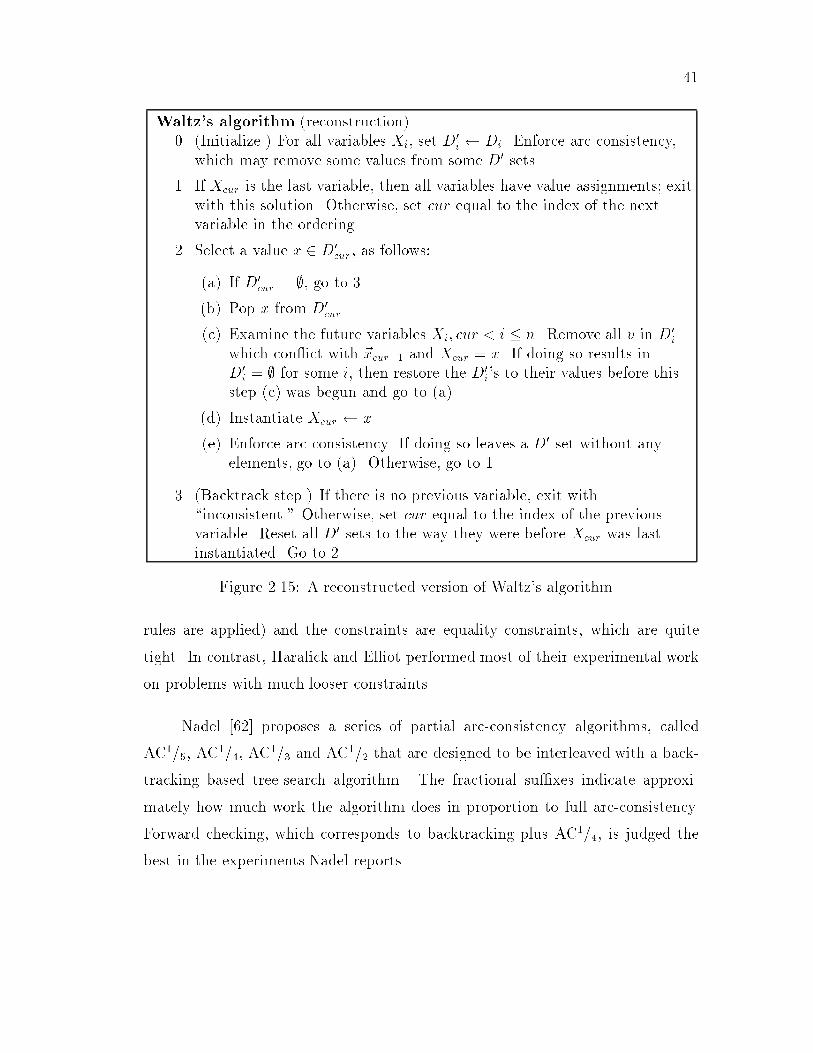
41

Waltz's algorithm (reconstruction)0. (Initialize.) For all variables Xi, set D0

i Di. Enforce arc-consistency,which may remove some values from some D0 sets.

1. If Xcur is the last variable, then all variables have value assignments; exitwith this solution. Otherwise, set cur equal to the index of the nextvariable in the ordering.

2. Select a value x 2 D0cur, as follows:

(a) If D0cur = ;, go to 3.

(b) Pop x from D0cur.

(c) Examine the future variables Xi; cur < i � n. Remove all v in D0i

which con ict with ~xcur�1 and Xcur = x. If doing so results inD0

i = ; for some i, then restore the D0i's to their values before this

step (c) was begun and go to (a).

(d) Instantiate Xcur x.

(e) Enforce arc-consistency. If doing so leaves a D0 set without anyelements, go to (a). Otherwise, go to 1.

3. (Backtrack step.) If there is no previous variable, exit with\inconsistent." Otherwise, set cur equal to the index of the previousvariable. Reset all D0 sets to the way they were before Xcur was lastinstantiated. Go to 2.

Figure 2.15: A reconstructed version of Waltz's algorithm.

rules are applied) and the constraints are equality constraints, which are quite

tight. In contrast, Haralick and Elliot performed most of their experimental work

on problems with much looser constraints.

Nadel [62] proposes a series of partial arc-consistency algorithms, called

AC1=5, AC1=4, AC1=3 and AC1=2 that are designed to be interleaved with a back-

tracking based tree-search algorithm. The fractional su�xes indicate approxi-

mately how much work the algorithm does in proportion to full arc-consistency.

Forward checking, which corresponds to backtracking plus AC1=4, is judged the

best in the experiments Nadel reports.

42

2.11 Full and Partial Looking Ahead

In addition to forward checking, Haralick and Elliott [40] de�ned two algo-

rithms called partial looking ahead and full looking ahead which do more consis-

tency enforcing than forward checking and less than arc-consistency.

The additional processing done by full looking ahead is a limited form of arc-

consistency, in e�ect performing a single iteration of the AC-1's outer loop (see

Fig. 2.16). The full looking ahead subroutine can be called in step 2 (c) of forward

checking (Fig. 2.9), by modifying that step in the following manner:

2. (Choose a value.)

(c) (Forward checking style look-ahead.) Examine the future variablesXi; cur < i � n, For each v in D0

i, if Xi = v con icts with ~xcur thenremove v from D0

i; if D0i is now empty, go to (d) (without examining

other Xi's).(Additional looking ahead.)

i. If Algorithm = FLA, perform full-looking-ahead(i);

ii. Else if Algorithm = PLA, performpartial-looking-ahead(i).

To illustrate how full looking ahead works, suppose there are three future

variables, X25 with current domain fa; bg, X26 with current domain fa; bg andX27 with current domain fbg. Also suppose there is an inequality constraint (as

in graph coloring) between X25 and X26 and between X26 and X27. Full looking

ahead will process X25 and reject neither of its values, since they both have a

compatible value in the domain of X26. When full looking ahead processes X26, it

removes the value b because there is no allowable match for b in the domain of X27.

Arc-consistency would later go back and remove a from X25's domain, because it

no longer has a consistent match in X26's domain, but full looking ahead does not

do this.

Partial looking ahead [40] seems to have been proposed with the same general

motivation that inspired the new heuristics presented later in this chapter: a notion

43

full-looking-ahead(d)1 for i d + 1 to n2 for j d+ 1 to n3 revise(i; j)4 if D0

i = ;5 then return

Figure 2.16: The full looking ahead subroutine.

that it might be possible to do a bit less work than that done by full looking ahead,

and yet to achieve most of the bene�ts. This scheme employed by partial looking

ahead is to check each future variable only with those other future variables later

than it (see Fig. 2.17). Dechter and Pearl [18] note that partial looking ahead

performs directional arc-consistency at each step, and this observation may explain

the motivation for the original development of the algorithm. However, when using

dynamic variable ordering the order of uninstantiated variables is not known, and

so the set of variables which are \after" a future variable is essentially a random one.

Of course it is possible to de�ne an ordering for the uninstantiated variables, but

this ordering is unlikely to be the order in which variables are actually instantiated.

2.12 Variable Ordering Heuristics

In describing the algorithms in the previous sections, we have assumed that

the order of the variables is static, that is, unchanging as the algorithm proceeds. In

partial-looking-ahead(d)1 for i d + 1 to n2 for j i+ 1 to n3 revise(i; j)4 if D0

i = ;5 then return

Figure 2.17: The partial looking ahead subroutine.

44

practice this is not necessarily the case, which requires modifying some algorithms.

In this section we �rst consider several heuristics for static variable ordering, and

then the dynamic variable ordering scheme most frequently used.

Waltz [90] proposed a variable ordering heuristic, motivated by the desire to

\eliminate as many possibilities as early as possible." First, label junctions on the

scene/background border, since those junctions tend to have few possible labels.

Second, label junctions which share an edge with those junctions in the �rst step.

In general constraint satisfaction terms, we can interpret these guidelines as \select

a variable which has few values" (e.g. jD0j is small). Intuitively, if we want the

size of the search tree to be as small as possible, it is probably better to put nodes

with small branching factor �rst.

In some application areas and in many instances of arti�cial data, all variables

have the same size domain. In such cases, static variable ordering schemes have to

rely on the constraint graph. We now present two which do so.

The minimum width (MW) heuristic [25] orders the variables from last to

�rst by selecting, at each stage, a variable in the constraint graph that connects

to the minimal number of variables that have not been selected yet. For instance,

in the CSP from Fig. 2.2, we could choose X2, X3 or X6 to be the last variable,

since each is connected to two other variables. If we arbitrarily select X2 to

be last, then X6 will be chosen to be second-to-last, since it now participates

in one constraint (X2 and constraints involving it having been eliminated), the

minimum. Now both X3 and X5 connect to two other nodes; we can choose

X5 to be third-to-last. Continuing in this manner, the �nal ordering might be

X7;X3;X1;X4;X5;X6;X2. There is usually more than one min width ordering

of a CSP.

The maximum cardinality (MC) variable ordering heuristic [17] selects the

�rst variable arbitrarily, and then selects each subsequent variable by choosing the

one connected with the largest number of previously chosen variables. A variation

45

of MC is to choose as the �rst variable the one that participates in the most

constraints. Using this variation, a maximum cardinality ordering of the variables

from Fig. 2.2 is X1;X2;X3;X7;X4;X5;X6.

The use of a variable ordering heuristic does not change the worst-case com-

plexity of any backtracking algorithm. The most extensive set of experiments

comparing the average case performance of MW and MC is reported in [17]. No

clear superiority between the two was discernable (several other ordering schemes

were studied as well), although MW was slightly superior.

Under a dynamic variable ordering scheme, the order of the variables is de-

termined as search progresses, and may be di�er from one branch of the search

tree to another. Most dynamic variable ordering heuristics are based on an idea

proposed by Haralick and Elliot [40] under the rubric \fail �rst." The main idea of

the heuristic is to select the future variable with the smallest remaining domain,

or D0 set. Haralick and Elliot show via a probabilistic analysis that choosing the

variable with the smallest number of remaining values minimizes the probability

that the variable can be consistently instantiated, and thus \minimizes the ex-

pected length or depth of any branch" (p. 308). The fail �rst heuristic relies on a

look-ahead technique such as forward checking to �lter the domains of the future

variables.

Several other dynamic variable ordering heuristics have been proposed. Those

of Purdom [71] and Minton et al. [56] do not rely on a forward checking style look

ahead, but most others do and can be considered variants of the Haralick and

Elliott's fail �rst principle: Nudel [65], Gent et al. [34].

Chapter 3

The Probability Distribution of

CSP Computational E�ort

3.1 Overview of the Chapter

In this chapter we present empirical evidence that the distribution of e�ort

required to solve CSPs can be approximated by two standard families of contin-

uous probability distribution functions1. Solvable problems can be modelled by

the Weibull distribution, and unsolvable problems by the lognormal distribution.

These distributions �t equally well over a variety of backtracking based algorithms.

We show that the mathematical derivation of the lognormal and Weibull distribu-

tion functions parallels several aspects of CSP search.

3.2 Introduction

This chapter reports our e�orts to uncover regularities that exist in the distri-

bution of e�ort required to solve CSPs, independent of the algorithm used (within

the framework of backtracking based algorithms) or the speci�c parameters to the

problem generating model. In all cases we consider satis�able and unsatis�able

1The general results and conclusions of this chapter were �rst reported in Frost et al. [29] and

Rish and Frost [73]

46

47

problems separately, since we have found them to have completely di�erent distri-

butions. For satis�able problems, we limit our attention to the e�ort required to

�nd the �rst solution.

The problem we address has long been an open one. Many researchers have

observed that the work required to solve constraint satisfaction problems exhibits

a large variance. Knuth noted in 1975 [46] that \great discrepancies in execution

time are characteristic of backtrack programs." Mitchell [57] writes \we can't

even estimate how large a sample size would be needed to obtain valid con�dence

intervals for the sample mean." Kwan [49] shows that the distribution of e�ort

on CSPs is not normal. Researchers have addressed the problem of unknown

distribution by reporting a variety of statistics, including the mean, the median,

the standard deviation, the minimum, the maximum, the 99th percentile, and the

99.9th percentile.

To illustrate the issues that may arise in reporting experimental results, con-

sider the data in Table 3.2, which come from an experiment using the BJ+DVO

algorithm (described in Chapter 4). The algorithm was applied to 10,000 random

instances created by a Model A generator and parameters h100; 8; :0566; 0:50i.Each line of the table reports various statistics { average, median, standard devi-

ation, maximum { after a certain number of instances had been processed. The

table is organized in this manner to show how the average hardness of a sample

of problems, measured by CPU time, can change as the size of the sample grows,

mostly due to the e�ect of rare very hard problems. Mitchell [57] reports a similar

table, based on an experiment with the Davis-Putnam procedure and random 3-

CNF formulas, in which at sample size 100 the mean is 98, and after 5,000 instances

the sample mean has become 12,000.

This pattern or distribution of problem hardness presents two sources of

di�culty for someone designing and reporting an experiment with a CSP algorithm

and randomly generated problems. The design question is, how many instances

are enough? The goal is to have the sample be representative of the entire set of

48

sample size average median hardest st. deviation50 12.08 3.18 60.60 32.44100 13.25 3.30 235.00 33.53200 17.33 3.62 290.83 45.37300 19.60 3.58 1,019.22 72.82400 19.28 3.42 1,019.22 69.16500 18.65 3.37 1,019.22 65.36800 20.31 3.42 1,176.63 71.85

1,000 18.96 3.32 1,176.63 67.591,500 18.00 3.16 1,176.63 69.652,000 20.20 3.08 3,083.43 101.495,000 19.26 3.13 3,083.43 88.9310,000 19.05 3.15 3,083.43 76.44

Table 3.1: Cumulative statistics at varying points in a 10,000 sample experi-ment. Units are CPU seconds, algorithm is BJ+DVO, generator parameters areh100; 8; :0566; 0:50i.

possible random problems with a certain set of parameters, requiring hundreds if

not thousands of instances. The example of Table 3.2 shows that with a sample

of a few hundred instances, the empirical mean can be about 10% too large or

too smal, if we make the assumption, perhaps unwarranted, that the sample mean

after 10,000 instances is close to the true population mean.

The second, related, question is which statistics to report. With more than

a few dozen instances it is not feasible to report the results of each instance. The

mean and the median are the most popular statistics to report, but these do not

convey the long \tail" of di�cult problems that often occurs. In order to con-

vey more information, some authors have reported percentile points such as the

hardness of the instance at the 99th and 99.9th percentiles, minimum and max-

imum values, and the standard deviation. In experiments involving large sets of

randomly generated instances, the ideal would be to report the entire distribution

of cost to solve. It might be imagined that doing so would be unwieldy. In this

chapter we present evidence that such an approach is quite feasible, because the

experimentally derived distributions are quite closely approximated by standard

distribution functions from the �eld of statistics.

49

Our main �ndings are that the hardness distributions of solvable and unsolv-

able problems are distinctly di�erent, with unsolvable problems being close to the

lognormal distribution, and solvable problems being reasonably well approximated

by the Weibull distribution. The lognormal and Weibull distributions are each

parameterized by shape and scale parameters. By noting that the results of an

experiment can be �t by a certain distribution with parameters x and y, it is pos-

sible to convey a complete understanding of the experimental results: the mean,

median, mode, variance, and shape of the tail.

We use the number of nodes in the search space to measure the computational

e�ort required to solve a problem instance. In [29] we measured consistency checks,

with almost identical results. A limitation of counting the number of nodes in the

search space as a proxy for overall e�ort of the algorithm is that this measure does

not take into account the amount of work, and ultimately CPU time, expended by

the algorithm at each node. This quantity can vary greatly; a theme of research

in CSP algorithms that we will explore in later chapters is how to best trade o�

extra work at some nodes for a su�ciently reduced size in the total search space.

Thus counting only the number of nodes is often not a fair comparison between

algorithms; this should be borne in mind when reading the tables which contain

results for multiple algorithms.

3.3 Random Problem Generators

3.3.1 Model A and Model B

In this chapter we use two random problem generators; following Smith and

Dyer [82] we call themModel A and Model B. In other chapters we use the Model B

generator only. In this chapter we focus on Model A because it has some properties

of independence between constraints which simpli�es the analysis at the end of the

chapter.

50

Both generators use parameters N , D, T , and C. N and D have the same

meaning in both models. As de�ned in Chapter 1, in Model B parameters C and T

de�ne the exactly number of constraints and prohibited value pairs per constraint.

In Model A, C is the probability of a constraint existing between any pair of

variables, and each constraint is statistically independent of the others. Parameter

T in Model A de�nes the probability that a value in the domain of one variable in

a constraint will be incompatible with a value in the domain of the other variable

in the constraint. Two di�erent problem instances under the Model A distribution

can have di�erent numbers of constraints, and two constraints in the model A

distribution can prohibit a di�erent number of value pairs.

3.3.2 Parameters at the Cross-over Point

The phase transition phenomenon, described in Chapter 1, is an important

aspect of empirical CSP research. In this and succeeding chapters, many experi-

ments are conducted with parameters at the cross-over point. Therefore, we brie y

discuss the manner in which we determined combinations of parameters values at

the cross-over point.

Two interesting aspects of the phase transition phenomenon are that the peak

in average di�culty occurs at the 50% satis�able point, and that the relationship

between the number of constraints and the number of variables at the cross-over

point is linear. Neither relationship has been proven analytically, but both have

been well established for K-SAT and for binary CSPs [12, 27, 35]. An accurate

formula for deriving sets of parameters at the cross-over point has not been found,

but the following equation, due to Smith [81] and Williams and Hogg [91], is an

approximation:

DN (1 � T )C0

= 1; (3:1)

DN is the total number of possible assignments of values to variables, and the

probability of any given random assignment satisfying all C 0 constraints is (1 �

51

D T formula for C 0

3 .111 7:300N + 16:723 .222 3:041N + 13:723 .333 1:516N + 15:563 .444 0:725N + 16:786 .111 13:939N + 12:826 .222 6:361N + 6:566 .333 3:761N + 5:496 .444 2:408N + 5:416 .556 1:510N + 7:009 .222 8:284N + 3:869 .333 4:949N + 4:879 .444 3:280N + 4:32

Table 3.2: Experimentally derived formulas for C 0 at the cross-over point, underModel B. C 0 = CN(N�1)=2 is the number of constraints in a CSP with parametersC and N .

T )C0

. The product is the expected number of solutions. When the expected

number of solutions is about 1, then the parameters are at the cross-over point.

The equation is not accurate because it makes an unwarranted assumption of

independence between the constraints, and because it ignores the distribution of

solutions. Solvable problems often have many solutions, so looking for the expected

number of solutions to be 1 is an approximation. Nevertheless, the formula does

describe the general relationship between the parameters at the cross-over point.

Equation (3.1) can be rewritten as

C 0 = N(�log1�T D); (3:2)

which shows that for �xed settings of T and D the relationship between C 0 and

N is linear. Similarly, (3.1) shows that for �xed N and D, increasing T means

decreasing C 0 to stay at the cross-over point; or for �xed N and T , D must increase

as C 0 decreases.

Because equation (3.1) is not accurate, the exact values of parameters at

the cross-over point have to be determined experimentally. Empirically derived

relationships between C 0 (number of constraints) and N (number of variables) are

52

given in Fig. 3.2, for selected values of D and T . These formulas were determined

through an iterative process. For a given set of parameters N , D, and T , 100

random problems were generated at each of several values of C. We used values of

C corresponding to an integer number of constraints. A standard CSP algorithm

was applied to each problem, and we noted the percentage that had solutions.

From that information we could estimate values of C reasonably near the cross-

over point. The process was repeated until the number of constraints at the cross-

over value was ascertained within one or two. We then ran experiments with

2,000 instances at each of two or three values of C. The �nal result was usually

one value of C that produced slightly more than 50% solvable, and one value

of C that produced slightly fewer. We determined the cross-over value of C by

linear interpolation. This is illustrated by the following example, for parameters

N=25;D=3; T=:111:

C 0 C solvable (out of 2,000)

198 0.6600 1058

199 0.6633 988

Interpolating linearly, 1,000 is .83 of the way from 1,058 to 988, so we estimate the

cross-over value of C 0 to be 198.83 in this example. When the cross-over values of

C 0 were determined for a �xed D and T and �ve to ten values of N , we derived

the parameters of the linear regression line using the Unix \pair" program [35].

3.4 Statistical Background

In this section we review some basic notions of statistics upon which the later

sections are based. We focus on three probability distributions, the normal, the

lognormal, and the Weibull.

53

3.4.1 Distribution functions

Given a random variable X, the probability distribution of X de�nes the

probability that X will take on any particular value in its domain. If X is a

continuous variable, then the probability distribution is a continuous probability

distribution. Although our study is of discrete constraint satisfaction problems,

we emphasize the continuous probability distributions to which they converge in

the limit of increased sample size.

The probability distribution of a continuous random variable X can be de-

�ned in two ways. The cumulative distribution function (cdf) F (x) speci�es the

probability that the value of X is less than or equal to x:

F (x) = P (X � x) (3:3)

The probability density function (pdf) f(x) is the derivative of the cumulative

probability function. Thus, for a continuous variable,

F (x) =Z x

�1f(t)dt (3:4)

and in particular

F (b)� F (a) =Z b

af(t) dt = P (a < X � b): (3:5)

For a continuous random variable X, the expected value E(X), also called

the mean, �, is given by

E(X) =Z 1

�1xf(x) dx; (3:6)

assuming the integral is absolutely convergent (jxjf(x)dx < 1). The deviation

from the mean of a particular value of X is (X � �). The expected value of the

square of the deviation is called the variance of X, and is written Var(X) or �2.

It is computed as

Var(X) = E[(X � �)2] = E(X2)� �2: (3:7)

The positive square root of the variance, �, is called the standard deviation.

54

3.4.2 Sample Statistics and Empirical Distributions

The arithmetic sample mean �x of n observations (x1; x2; . . . ; xn) is the sum

of all observations divided by the number of observations, or

�x =1

n

Xi

xi: (3:8)

The sample variance s2 is computed as

s2 =1

n� 1

Xi

(xi � �x)2 (3:9)

and the sample standard deviation s is the positive square root of s2.

The empirical distribution function is important for goodness-of-�t tests we

discuss in a later section. Let x1; x2; . . . ; xn denote an ordered random sample of

size n. The empirical distribution function, or sample CDF, is calculated as

Femp(xi) = i=n: (3:10)

Thus Femp ranges from 1=n to 1.

3.4.3 The normal distribution

Perhaps the most widely used distribution in statistics is the normal distri-

bution. The probability density function of the normal distribution is

f(x) =1

�p2�

exp

�(x� �)2

2�2

!: (3:11)

The pdf f(x) is parameterized by �, the mean of the distribution which has the

range �1 < � < 1, and �, the standard deviation of the distribution, which

ranges 0 < � < 1. The normal distribution with parameters � and � is de-

noted N(�; �2). The standardized normal distribution, N(0; 1), has a cumulative

distribution function �(x) de�ned by

�(x) =1p2�

Z 1

�1e�

1

2 t2 dt (3:12)

55

In general, if z = (x� �)=� then F (x) = �(z).

Much of the usefulness of the normal distribution stems from the fact that,

in the limit, the sum of independent random variables tends to be normally dis-

tributed. This is known as the central limit theorem.

Theorem 1 (Central Limit Theorem) Let (X1;X2; . . .) be a sequence of inde-

pendent random variables with cdf's (F1(X); F2(X); . . .), means (�1; �2; . . .), and

variances (�21; �22; . . .). Let an = X1 + � � � + Xn, �n = �1 + � � � + �n, and � 2n =

�21 + � � �+ �2n. Then

limn!1P

an � �n�n

< y

!= �(y); (3:13)

or in other words

limn!1 dn is distributed as N(�n; �

2n) (3:14)

subject to certain conditions on the variances �2i .

3.4.4 The lognormal distribution

A positive random variable X is lognormally distributed with parameters �

and � if Y = lnX is normally distributed with mean � and variance �2. We say

X is distributed as �(�; �2). The probability density function of the lognormal is

f(x) =

8><>:

1p2��x

exp�� (lnx��)2

2�2

�; x > 0

0; x � 0:(3:15)

The parameters � and � are not the mean and standard deviation of the lognormal

distribution. These statistics, and the variance, median and mode, are given by

E(X) = exp(�+ �2=2) (3.16)

StdDev(X) = exp(�)(exp(2�2)� exp(�2))1=2 (3.17)

Var(X) = exp(2�+ �2)(exp(�2)� 1) (3.18)

Median(X) = exp(�) (3.19)

Mode(X) = exp(�� �2) (3.20)

56

0 2 4 6

.2

Density

a

b c

lognormal� � mean

a 0.63 1.0 3.08

b 1.00 1.0 4.48

c 1.00 0.5 3.08

0 1 2 3

1d

ef

Weibull� � mean

d 1.0 1.0 1.00

e 1.0 0.5 2.00

f 1.0 2.0 0.89

Figure 3.1: Graphs of the lognormal and Weibull density functions for selectedparameter values.

The cumulative distribution function of the lognormal is

F (x) = �

lnx� �

�

!: (3:21)

The �rst graph in Fig. 3.1 shows the shape of the lognormal pdf for several values

of � and �. When � is small the pdf is relatively symmetric and the mean and

median are close together. As � increases, the lognormal distribution becomes

more skewed, and the probability of a random instance being above the mean

decreases.

3.4.5 The Weibull distribution

The Weibull distribution has wide applicability in reliability and lifetime

studies. Its probability density function is

f(x) =

8><>:

���x��1e�(�x)�

; x > 0

0; x � 0(3:22)

and the cdf is

F (x) =

8><>:

1 � e�(�x)�

; x > 0

0; x � 0:(3:23)

57

The parameter � is interpreted as scale and � as shape. The mean, E, of a Weibull

distribution is given by E = ��1�(1 + ��1) where �(�) is the Gamma function.

There is also a three parameter version of the Weibull distribution, in which x is

replaced by x�� in the above equations; � is called the origin of the distribution.

When � = 1, the Weibull distribution is identical to the exponential distribution.

The second graph in Fig. 3.1 shows the shape of the Weibull pdf for several

values of � and �. When � � 1, the pdf has no mode (maximum value) and

is monotonically decreasing. When � is greater than 1, the pdf has a maximum

which is greater than 0; the greater is �, the further to the right on the graph the

maximum appears.

3.4.6 Statistical Signi�cance and Tail Ratio Test

It is important to be able to measure and report the goodness of �t between

a hypothesized distribution function and a sample created experimentally. We

measure the discrepancy in two ways, with a standard statistical technique called

the Kolmogorov-Smirnov statistic, and with a measure we developed call the Tail

Ratio.

The Kolmorgorov-Smirnov (KS) test statistic is based on the maximum dif-

ference between the cdf of the hypothesized distribution and the empirical cdf of

the sample. Let F (x) be the cdf of the hypothesized distribution, and de�ne

D+ = maxi(i=n � F (xi)) = max

i(Femp(xi)� F (xi))

D� = maxi(F (xi) � (i� 1)=n) = max

i(F (xi)� Femp(xi�1))

Dmax = max(D+;D�):

D+ is the maximumdistance the empirical cdf goes above the hypothesized cdf, and

D� is the maximum distance below. Fig. 3.2 shows the cdf for the lognormal with

� = 12:00 and � = 0:44. Fig. 3.3 shows a small section of an empirical distribution

based on a sample and which demonstratesDmax visually. Dmax is the KS statistic;

58

132,111 400,000 600,000

.1

.5

.9

Figure 3.2: The cumulative distribution function for �(12:00; 0:44) (see the �fthline in Fig. 3.6). The curve is truncated at (F (646650) = 0:99. The small squareindicates the portion magni�ed in the next Figure. 132,111 is the median of thedistribution.

we report it in tables under the heading \KS". This value can range from 0 to 1,

with a smaller value indicating a better �t. In general terms, when the product

of the KS statistic and the square root of the number of samples is less than 1, a

close match between the distribution and the sample is indicated. To interpret the

statistical signi�cance of the KS statistic, it is necessary to know critical values

that correspond to particular level of signi�cance. If speci�c parameters of the

distribution are part of the hypothesis that is being tested, then these critical

values are readily available. In our case, however, the distribution parameters are

estimated from the sample data, and there is no simple way to derive critical values.

We report the KS statistic solely as an indicator of the relative goodness-of-�t of

di�erent samples to the corresponding lognormal or Weibull functions.

The KS statistic is not particularly sensitive at the tails of the distribution,

since at these points both the hypothesized distribution and the sample's empirical

distribution tend to come together at 0 or 1. Indeed, we have found that Dmax

is usually found near the median of the sample. Sometimes experimenters are

particularly interested in the behavior of the rare hard problems in the right tail.

Therefore, we have devised a measure called the Tail Ratio (TR) which focusses

59

132,111130,000

.49

.50

.51

Dmax

Figure 3.3: Computing the KS statistic Dmax, when comparing the cdf for�(12:00; 0:44) (smooth line) and the empirical cdf for the experiment describedin the �fth row of Fig. 3.6 (stepwise line). Note that only a small part of the curvenear the maximum di�erence is shown.

on the goodness-of-�t in the right tail of the distribution. In general, the tail ratio

of two distributions with cdfs F1 and F2 is parameterized by a value �, and is

the ratio of probabilities that a random variable will be greater than � in each

distribution:

TR� = (1� F1(�))=(1 � F2(�)): (3:24)

In practice, we always set � equal to the number of nodes explored for the sample

instance at the 99th percentile. For example, out of 5,000 instances the 4,950th

hardest one might require 2,000,000 nodes, so � = 2;000;000. F1 is the cdf of the

lognormal or Weibull function, and F2 is the empirical distribution function for

the sample. Because of the way � is selected, F2(�) = :99. Thus,

TR =1 � F (99th percentile in sample)

1� :99(3:25)

where F is the appropriate cdf. If the TR is 1.0, the match is perfect and the

distribution accurately models the 99th percentile of the right tail. A number less

than 1 indicates that the distribution does not predict as many hard instances as

60

were actually encountered; when greater than 1 the TR indicates the distribution

predicts too many hard instances.

3.4.7 Estimating Distribution Parameters

The �eld of statistics has developed methods for estimating the parameters of

a distribution from sample values. It is almost always assumed that the distribution

function is known. The \universal method for optimal estimation of unknown

parameters" [75] is the maximum likelihood method, which chooses parameter

values which maximize the probability that the observed sample would occur.

For the lognormal distribution we use the maximum likelihood estimator

(MLE) [11]. Let fx1; x2; . . . ; xng be the n samples. The estimate of �, called �̂,

and of �2, called �̂2, are computed as

�̂ =1

n

nXi=1

lnxi (3.26)

�̂2 =1

n

nXi=1

(lnxi � �̂)2: (3.27)

The MLE for the Weibull distribution is not recommended when � < 2 [11],

which is usually the case for the data we encounter

We therefore use a modi�ed moment estimator (MME) [11]. Again, let the

n samples be fx1; x2; . . . ; xng, with x1 the smallest in the set. Let �x be the sample

mean, s2 be the sample variance, and �̂; �̂ and �̂ be the estimates for the Weibull

parameters. Where �(�) is the Gamma function, let

�̂k = �

1 +

k

�̂

!: (3:28)

The �rst step of the MME is to iterate over possible values of �̂, �nding a value

which satis�es the equality

s2

(�x� x1)2=

�̂2 � �̂21�

(1� n�1=�̂)�̂1

�2 : (3:29)

61

We varied �̂ from 0.010 to 2.000 in steps of .001, selecting the value that minimized

the di�erence between the two sides in (3.29). With �̂ derived, the MME computes

the other parameters as

�̂ =sq

�̂2 � �̂21

(3.30)

�̂ = �x� �̂�̂1: (3.31)

3.5 Experiments

The primary goal of the experiments is to show the goodness-of-�t between

the empirical distributions of the samples and the lognormal (for unsolvable prob-

lems) and Weibull (for solvable problems) distributions. We use both Model A

and Model B random problem generators. We view the random CSP generator as

de�ning a distribution over the set of all CSPs. This distribution is a distribution

over CSP instances, not over the work to process these instances. For a given set

of parameters hN;D;C; T i, CSPs which cannot be output by the generator have

a probability of 0 in the distribution, while all CSPs which can be generated have

an equal probability under the distribution.

Model B has been more widely used in recent empirical studies of CSP algo-

rithms than Model A. The advantage of Model A, for the purposes of this chapter,

is that the independence of constraints and prohibited value pairs simpli�es the

analysis of why the lognormal distribution appears in unsatis�able problems. We

discuss this topic in section 3.6.

Because there are many experiments to report, we start with an outline of the

section. In subsection 3.5.1 we show that the distributions are observed under a va-

riety of algorithms; the experiments in this section use Model A with combinations

of parameters that are at or near the 50% solvable cross-over point. Section 3.5.2

show how increasing the sample size, from 100 up to 1,000,000 instances, reduces

62

Search Space Nodes

Freq.

h20,6,.9789,.167iModel A, BT+RND� = 13:21; � = 0:53KS: 0.0046 TR: 1.1

627,5830 2,510,200

.010

.020

Search Space Nodes

Freq.

h20,6,.7053,.222iModel A, BT+RND� = 13:21; � = 0:85KS: 0.0076 TR: 0.9

787,7500 3,150,800

.010

.020

Figure 3.4: Graphs of sample data (vertical bars) and the lognormal distribution(curved line). Based on the unsolvable portion of 20,000 instances for each graph.Algorithm is simple backtracking with random variable ordering (BT+RND).

the seemingly random uctuations in the histogram bars in the graphs. In sub-

section 3.5.3, we show that empirical distributions can also be approximated by

the lognormal and Weibull functions outside the 50% satis�able region as well.

Subsection 3.5.4 shows the impact of using Model B on the goodness-of-�t.

Throughout our experiments we employ the same procedures and report the

data in a consistent format. Our experimental procedure consisted of selecting var-

ious sets of parameters for the random CSP generator, then generating 20,000 or

more instances for each set, and applying one or more search algorithms to each in-

stance. For each instance and algorithm we recorded whether a solution was found

63

Search Space Nodes

Freq.

h20,6,.4263,.333iModel A, BT+RND� = 13:38; � = 1:29KS: 0.0076 TR: 0.9

1,531,5000 6,126,000

.01

.02

.03

Search Space Nodes

Freq.

h20,6,.2316,.500iModel A, BT+RND� = 14:08; � = 1:94KS: 0.0096 TR: 0.7

9,767,8570 39,086,600

.05

.10

.15

Figure 3.5: Continuation of Fig. 3.4, with di�erent problem generator parameters.

and the number of nodes in the search space. We derived parameters for the distri-

butions, and measured the closeness of the �t using the KS (Kolmogorov-Smirnov)

and TR (Tail Ratio) statistics. Each line in Fig. 3.3 and Fig. 3.4 represents one

experiment with one algorithm on the unsolvable (Fig. 3.3) or solvable (Fig. 3.4)

instances generated from one set of parameters. The column labeled \Mean" in

these tables shows the mean number of nodes for an experiment. The \�", \�",

\�", \�", and \�" columns show the estimated value for these parameters. Since

values for � are typically very small, we show themmultiplied by 106. In the \solv"

column is the percentage of solvable problems that were generated with the given

64

parameters. The \KS" column holds the Kolmogorov-Smirnov statistic, and the

tail ratio measure is reported in the \TR" column.

We also show some experimental results and distributions in a pictorial fash-

ion, as in Fig. 3.4, Fig. 3.5, Fig. 3.6, and Fig. 3.7. These graphs can be di�cult

to interpret, because each one has its own scale for the x and y axes. The sample

data is represented by a histogram of vertical bars. The samples in each case have

been grouped into 200 bins; a problem that required between (i� 1) � w + 1 and

i�w nodes is reported in the ith bin. The \width" of the bin, w, is set to be equal

to one-�ftieth of the mean, unless noted otherwise. When this is so the sample

mean, which is noted on the x-axis, is one fourth of the way across the graph, from

left to right. Instances greater than four times the mean are not pictured, but

are considered in estimating the parameters. The height of each vertical line is in

proportion to the fraction of the sample that fell within the corresponding range

of nodes, as indicated on the y-axis. The continuous line on the charts indicates

the distribution function; the height of the line at i, 0 < i � 200, is proportional

to F (i � w) � F ((i � 1) � w), where F is the cdf and w is the bin width. The

vertical dotted lines indicate the median and 90th percentile of the data.

For example, in the top graph of Fig. 3.4, the mean of the 12,125 unsolvable

instances was 627,583. Dividing the mean by 50 and ignoring the remainder yields

a bin width, w, of 12,551. The 100th bin, to focus on one in particular, contains 34

samples which required between 1,242,550 and 1,255,100 nodes in the search. The

height of the histogram line representing bin 100 is therefore 34=12125 = 0:002804.

Using the lognormal cdf F with parameters � = 13:21 and � = 0:53, the height of

the curved line at x = 100 is F (1225100) � F (1242550) = 0:941210 � 0:938968 =

0:002242. Since 0:002242 < 0:002804, at this point along the x-axis the vertical

line extends above the curved line. Samples above 200� 12551 = 2510200 are not

shown on the graph. There were 17 such instances in this experiment, ranging

from 2,583,312 to 5,024,460. Truncating the extreme right tails of the graphs is

65

Modelh N, D, C, T i Unsolvable / LognormalParameters Mean � � solv KS TR

Algorithm: BT+RNDA h20, 6, .9789, .167i 627,583 13.21 0.53 39% 0.0046 1.1A h20, 6, .7053, .222i 787,750 13.21 0.85 40% 0.0076 0.9A h20, 6, .4263, .333i 1,531,500 13.38 1.29 42% 0.0111 0.9A h20, 6, .2316, .500i 9,601,654 14.08 1.94 43% 0.0096 0.7Algorithm: BJ+RNDA h20, 6, .9789, .167i 180,251 12.00 0.44 39% 0.0077 1.0A h20, 6, .7053, .222i 167,360 11.79 0.68 40% 0.0078 0.9A h20, 6, .4263, .333i 149,273 11.41 0.99 42% 0.0096 0.8A h20, 6, .2316, .500i 117,744 10.68 1.36 43% 0.0122 1.4Algorithm: FC+RNDA h20, 6, .9789, .167i 9,421 9.05 0.45 39% 0.0036 1.0A h20, 6, .7053, .222i 8,477 8.81 0.68 40% 0.0071 0.9A h20, 6, .4263, .333i 8,659 8.49 1.05 42% 0.0124 0.7A h20, 6, .2316, .500i 20,296 8.34 1.66 43% 0.0189 0.5Algorithm: BT+MWA h20, 6, .9789, .167i 509,301 13.01 0.51 39% 0.0058 1.0A h20, 6, .7053, .222i 85,687 11.19 0.57 40% 0.0096 0.8A h20, 6, .4263, .333i 17,855 9.50 0.75 42% 0.0129 0.8A h20, 6, .2316, .500i 4,381 7.90 0.93 43% 0.0218 0.9Algorithm: BJ+DVOA h20, 6, .9789, .167i 639 6.42 0.29 39% 0.0073 1.1A h20, 6, .7053, .222i 321 5.71 0.35 40% 0.0068 1.0A h20, 6, .4263, .333i 136 4.81 0.46 42% 0.0128 0.8A h20, 6, .2316, .500i 53 3.78 0.58 43% 0.0357 0.4

Table 3.3: Goodness-of-�t between unsolvable CSP instances and the lognormaldistribution. This table compares a variety of algorithms.

unfortunate but essential for maintaining a scale appropriate to the rest of the

graph.

3.5.1 First Set of Experiments: Variety of Algorithms

The �rst set of experiments are designed to explore how well the lognormal

and Weibull distributions �t the data over a range of settings of C and T , and for

66

Search Space Nodes

Freq.

h20,6,.9789,.167iModel A, BT+RND� = 3:17e� 06; � = 1:01; � = 20KS: 0.0173 TR: 1.0

313,2620 1,253,000

.010

.020

Search Space Nodes

Freq.

h20,6,.7053,.222iModel A, BT+RND� = 2:54e� 06; � = 0:78; � = 20KS: 0.0289 TR: 0.8

454,9880 1,819,800

.025

.050

Figure 3.6: Graphs of sample data (vertical bars) and the Weibull distribution(curved line). Based on the solvable portion of 20,000 instances for each graph.Algorithm is simple backtracking with random variable ordering (BT+RND).

a variety of algorithms. We set N=20 and D=6, and chose four combinations of T

and C which result in a roughly equal number of solvable and unsolvable instances.

The algorithms used are all based on backtracking search and are described in detail

in Chapter 2. The basic algorithm, backtracking, can be run with a �xed random

variable ordering (BT+RND) or using the min-width variable ordering heuristic

(BT+MW). We also experiment with backjumping and a random variable ordering

(BJ+RND) and forward checking with random variable ordering (FC+RND). We

selected a variety of relatively simple algorithms in order to demonstrate that the

correspondence with continuous distributions is not the consequence of any speci�c

67

Search Space Nodes

Freq.

h20,6,.4263,.333iModel A, BT+RND� = 1:50e� 06; � = 0:60; � = 19KS: 0.0564 TR: 0.4

1,004,7480 4,018,800

.05

.10

Search Space Nodes

Freq.

h20,6,.2316,.500iModel A, BT+RND� = 3:61e� 07; � = 0:42; � = 19KS: 0.1193 TR: 0.7

8,381,0830 33,524,200

.1

.2

.3

Figure 3.7: Continuation of Fig. 3.6.

heuristic, but holds for many varieties of backtracking search. As an example

of a sophisticated variation of backtracking search that combines backjumping,

forward checking style look-ahead, and a dynamic variable ordering heuristic, we

use BJ+DVO, described in chapter 4.

The results of the experiments are presented in Table 3.3 (unsolvable prob-

lems) and Table 3.4 (solvable problems). The results for the experiments with

BT+RND are shown graphically in Fig. 3.4, Fig. 3.5, Fig. 3.6, and Fig. 3.7.

The �t between unsolvable problems and the lognormal distribution is quite

good. It is least good for the problems with parameters h20; 6; :2316; :500i, which

68

have the sparsest graphs and the tightest constraints. For the other sets of param-

eters, the TR statistic ranges from 0.7 to 1.1, and KS is not greater than 0.0129.

Fig. 3.4 and Fig. 3.5 show visually that the lognormal distribution accurately re-

ects the shape of the data.

The �t between the Weibull distribution and the distribution of solvable

problems is much less good, but not entirely unsatisfactory. The visual evidence in

Fig. 3.6 and Fig. 3.7 is that the �t is good enough to use the Weibull distribution

for capturing the overall shape of the empirical distribution. The �t is least good to

the \left" of the median line, where the Weibull distribution is often substantially

larger or smaller than the observed value. It is possible to choose parameters

for the Weibull distribution which create a closer �t on the easiest problems (the

left part of the graph), but these parameters always cause an extreme mismatch

between the Weibull and empirical distributions elsewhere on the graph.

We observe a pattern that holds for both solvable and unsolvable problems:

the sparser the constraint graph, the greater the variance of the distribution, in-

dicated by larger � and smaller �. The e�ect is visible in Table 3.3 and Table 3.4

when comparing rows with the same N, D, and algorithm. Parameters T and C

are inversely related at the 50% satis�able point, so the e�ect may be due to in-

creasing T as well. The pattern holds even with BT. BJ, FC, and BT+MW can

exploit tight constraints and a sparse graph to make such problems much easier.

BT does not, but we still �nd greater variance with lower C.

69

Modelh N, D, C, T i Solvable / WeibullParameters Mean �� 106 � � solv KS TR

Algorithm: BT+RNDA h20, 6, .9789, .167i 313,262 3.17 1.01 19 39% 0.0173 1.0A h20, 6, .7053, .222i 454,988 2.54 0.78 19 40% 0.0289 0.6A h20, 6, .4263, .333i 1,004,748 1.50 0.60 19 42% 0.0564 0.4A h20, 6, .2316, .500i 8,248,756 0.36 0.42 19 43% 0.1193 0.7Algorithm: BJ+RNDA h20, 6, .9789, .167i 85,121 11.39 1.08 19 39% 0.0202 1.4A h20, 6, .7053, .222i 82,993 12.94 0.87 19 40% 0.0142 0.7A h20, 6, .4263, .333i 72,204 17.78 0.69 19 42% 0.0307 0.6A h20, 6, .2316, .500i 45,942 37.92 0.54 19 43% 0.0696 0.5Algorithm: FC+RNDA h20, 6, .9789, .167i 4,794 200.34 1.12 19 39% 0.0158 1.3A h20, 6, .7053, .222i 4,920 214.65 0.89 19 40% 0.0155 0.7A h20, 6, .4263, .333i 5,810 219.69 0.69 19 42% 0.0388 0.5A h20, 6, .2316, .500i 18,129 132.14 0.46 19 43% 0.1014 0.7Algorithm: BT+MWA h20, 6, .9789, .167i 246,677 3.99 1.04 19 39% 0.0144 1.0A h20, 6, .7053, .222i 46,478 21.99 0.95 19 40% 0.0120 0.8A h20, 6, .4263, .333i 11,798 94.48 0.82 19 42% 0.0207 0.6A h20, 6, .2316, .500i 9,899 163.89 0.57 19 43% 0.1833 4.0Algorithm: BJ+DVOA h20, 6, .9789, .167i 324 2,817 1.41 0 39% 0.0276 1.4A h20, 6, .7053, .222i 182 5,008 1.38 0 40% 0.0322 1.1A h20, 6, .4263, .333i 91 10,035 1.39 0 42% 0.0741 0.5A h20, 6, .2316, .500i 47 19,478 1.46 0 43% 0.1631 0.1

Table 3.4: Goodness-of-�t between solvable CSP instances and the Weibull distri-bution. This chart compares a variety of algorithms.

3.5.2 1,000,000 instances

In the this section we report on an experiment in which almost two million

CSP instances { approximately 1,000,000 unsolvable instances { were created and

processed with the BJ+DVO algorithm. The goal was to explore visually the e�ect

of varying the number of samples in a chart. One di�culty in interpreting charts

such as those in Figs. 3.4 and 3.5 is the uctuations in the heights of the histogram

bars. Apparently more samples are necessary to smooth the histogram.

70

Search Space Nodes0 3,000 6,000

.01

.02

.03

.04

.05

.06

Search Space Nodes

Freq.

0 3,000 6,000

.01

.02

Figure 3.8: Unsolvable problems from parameters h50; 6; :1576; :333i, using algo-rithm BJ+DVO. The top chart is based on the �rst 100 unsolvable instances, thebottom chart on the �rst 1,000 unsolvable instances. Each histogram bar repre-sents the number of sample instances in a range of 30 nodes.

The parameters used in this experiment were h50; 6; :1576; :333i, and only

unsolvable instances are reported. The relevant charts are in Fig. 3.8 through

Fig. 3.12. The samples displayed are cumulative; e.g. the 100 instances in the top

chart of Fig. 3.8 are also included in the bottom chart, along with the next 900 in

the experiment.

71

Search Space Nodes

Freq.

0 3,000 6,000

.005

.010

.015

Search Space Nodes

Freq.

0 3,000 6,000

.005

.010

.015

Figure 3.9: Continuation of Fig. 3.8. The top chart is based on the �rst 10,000unsolvable instances, the bottom chart on the �rst 100,000 unsolvable instances.

72

Search Space Nodes

Freq.

0 1,000 3,000 6,000

.005

.010

.015

Figure 3.10: Continuation of Fig. 3.8 and Fig. 3.9. This chart is based on 1,000,000unsolvable instances.

Figs. 3.8, 3.9, and 3.10 show histograms and lognormal distributions based

on samples of sizes 100, 1,000, 10,000, 100,000, and 1,000,000. In each chart the

same x-axis scale is used { one histogram bar represents a range of 30 nodes.

The distributions are truncated above 6,000 nodes, so there are 200 bars in each

chart. The y-axis scales are the same within each �gure, but change from �gure to

�gure. In each chart, the lognormal distribution pictured is based on parameters

estimated from that chart's sample.

The top chart in Fig. 3.8 is based on 100 instances, and so displays many

gaps in the histogram. Most of the histogram bars have a height of 0.00 (that

is, no bar) or 0.01, because exactly zero or one instance (out of one hundred) fell

into the corresponding range. With 100 instances the chart looks awful, and it is

nearly impossible to tell by eye the goodness-of-�t between the sample data and

the lognormal distribution display. If this were the only set of data to display,

clearly a better scale could be chosen.

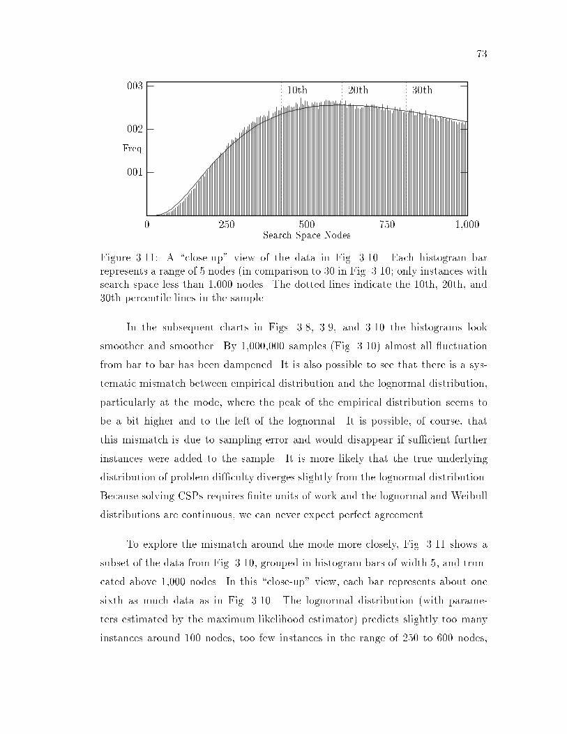
73

Search Space Nodes

Freq.

0 250 500 750 1,000

10th 20th 30th

.001

.002

.003

Figure 3.11: A \close-up" view of the data in Fig. 3.10. Each histogram barrepresents a range of 5 nodes (in comparison to 30 in Fig. 3.10; only instances withsearch space less than 1,000 nodes. The dotted lines indicate the 10th, 20th, and30th percentile lines in the sample.

In the subsequent charts in Figs. 3.8, 3.9, and 3.10 the histograms look

smoother and smoother. By 1,000,000 samples (Fig. 3.10) almost all uctuation

from bar to bar has been dampened. It is also possible to see that there is a sys-

tematic mismatch between empirical distribution and the lognormal distribution,

particularly at the mode, where the peak of the empirical distribution seems to

be a bit higher and to the left of the lognormal. It is possible, of course, that

this mismatch is due to sampling error and would disappear if su�cient further

instances were added to the sample. It is more likely that the true underlying

distribution of problem di�culty diverges slightly from the lognormal distribution.

Because solving CSPs requires �nite units of work and the lognormal and Weibull

distributions are continuous, we can never expect perfect agreement.

To explore the mismatch around the mode more closely, Fig. 3.11 shows a

subset of the data from Fig. 3.10, grouped in histogram bars of width 5, and trun-

cated above 1,000 nodes. In this \close-up" view, each bar represents about one

sixth as much data as in Fig. 3.10. The lognormal distribution (with parame-

ters estimated by the maximum likelihood estimator) predicts slightly too many

instances around 100 nodes, too few instances in the range of 250 to 600 nodes,

74

Search Space Nodes

Freq.

6,000 9,000 12,000

97th 98th 99th

.0001

.0002

.0003

.0004

.0005

Search Space Nodes

Freq.

12,000 15,000 18,000

99.7th 99.9th

.00001

.00002

.00003

.00004

.00005

Figure 3.12: The two graphs are continuations of Fig. 3.10, showing data in thetail of the distributions. The top chart extends Fig. 3.10 from 6,000 to 12,000nodes, and the bottom chart continues from 12,000 to 18,000 nodes. The x-axisscale is the same in Fig. 3.10 and these charts { 30 nodes, but the vertical scalevaries. The dotted lines show the indicated percentiles in the sample.

75

sample size sample mean � �

50 1,703 6.969 1.046100 1,723 7.012 0.981

1,000 1,971 7.192 0.88510,000 1,913 7.173 0.876100,000 1,912 7.172 0.879

1,000,000 1,914 7.173 0.880

Table 3.5: Mean number of nodes and estimated values of � and � for the lognormaldistribution, using the maximum likelihood estimator, based on varying samplesizes.

and just about the right number from 600 to 1,000 nodes. The visual evidence,

from this one experiment, is that the sample is not drawn from an exactly log-

normal distribution, but that the approximation is su�ciently close for almost all

purposes.

In Fig. 3.12 we show some of the tail of the distribution with 1,000,000

instances. This �gure should be viewed as a continuation of Fig. 3.10, extending

the chart to those instances with a search space of 6,000 to 12,000 nodes (top chart)

and 12,000 to 18,000 nodes (bottom chart). The x-axis scale of the three charts

is identical (30 nodes), but the y-axis scales are modi�ed as appropriate. Again

the goodness-of-�t of the lognormal seems quite good to the eye, although above

the 99.7th percentile it seems to be overestimating slightly the actual number of

instances.

It is interesting to observe how the maximum likelihood estimates of the

lognormal parameters change as the sample size increases. This data is tabulated

in Table 3.5. The estimates of � and � are reasonably accurate after even 50

samples, and by 1,000 samples they are almost identical to their values at 1,000,000

instances.

3.5.3 Parameters not at the cross-over point

76

Modelh N, D, C, T i Unsolvable / LognormalParameters Mean � � solv KS TR

Algorithm: BJ+DVOA h20, 6, .5263, .222i 27,906 9.93 0.79 99% 0.1147 1.0A h20, 6, .5526, .222i 21,390 9.70 0.72 99% 0.0623 0.1A h20, 6, .5789, .222i 18,138 9.52 0.75 98% 0.0327 0.7A h20, 6, .6053, .222i 16,595 9.44 0.73 94% 0.0176 0.6A h20, 6, .6316, .222i 14,231 9.29 0.73 86% 0.0168 0.7A h20, 6, .6579, .222i 11,947 9.13 0.71 73% 0.0078 0.8A h20, 6, .6842, .222i 10,014 8.96 0.69 55% 0.0114 0.9A h20, 6, .7105, .222i 8,279 8.78 0.69 37% 0.0094 0.9A h20, 6, .7368, .222i 6,544 8.55 0.67 22% 0.0109 0.8A h20, 6, .7632, .222i 5,175 8.33 0.65 11% 0.0145 1.0A h20, 6, .7895, .222i 4,043 8.11 0.62 5% 0.0141 0.7A h20, 6, .8158, .222i 3,122 7.87 0.58 2% 0.0136 0.6A h20, 6, .8421, .222i 2,458 7.65 0.55 1% 0.0147 0.6A h20, 6, .8684, .222i 1,946 7.44 0.51 0% 0.0148 0.7A h20, 6, .8947, .222i 1,574 7.25 0.47 0% 0.0102 0.8A h20, 6, .9211, .222i 1,295 7.07 0.44 0% 0.0126 0.8A h20, 6, .9474, .222i 1,078 6.90 0.41 0% 0.0082 0.7A h20, 6, .9737, .222i 908 6.74 0.38 0% 0.0065 0.8A h20, 6, 1.000, .222i 773 6.59 0.34 0% 0.0029 0.9

Table 3.6: Goodness-of-�t for a set of experiment with �xed values for N , D andT and varying values of C. Unsolvable problems; algorithm is FC+RND.

77

Modelh N, D, C, T i Solvable / WeibullParameters Mean � � solv KS TR

Algorithm: BJ+DVOA h20, 6, .5000, .222i 1,700 1,176.75 0.50 100% 0.0537 0.8A h20, 6, .5263, .222i 2,065 861.27 0.54 99% 0.0342 0.6A h20, 6, .5526, .222i 2,587 614.72 0.58 99% 0.0352 0.7A h20, 6, .5789, .222i 3,221 444.70 0.62 98% 0.0257 0.7A h20, 6, .6053, .222i 3,827 339.84 0.68 94% 0.0187 0.8A h20, 6, .6316, .222i 4,597 263.44 0.74 86% 0.0154 0.7A h20, 6, .6579, .222i 4,849 215.65 0.87 73% 0.0154 0.7A h20, 6, .6842, .222i 4,981 218.92 0.94 55% 0.0174 0.7A h20, 6, .7105, .222i 4,696 217.47 0.95 37% 0.0168 0.7A h20, 6, .7368, .222i 4,412 231.24 0.96 22% 0.0186 0.6A h20, 6, .7632, .222i 3,876 256.53 1.01 11% 0.0314 0.5A h20, 6, .7895, .222i 3,162 311.33 1.04 5% 0.0393 0.7A h20, 6, .8158, .222i 2,748 351.12 1.10 2% 0.0384 1.1A h20, 6, .8421, .222i 2,221 441.03 1.05 1% 0.0538 0.5

Table 3.7: Goodness-of-�t for a set of experiment with �xed values for N , D andT and varying values of C. Solvable problems; algorithm is FC+RND.

In the previous experiments the parameters were selected such that ap-

proximately equal numbers of solvable and unsolvable instances were generated.

Parameters at the cross-over point are used by many experimenters when eval-

uating algorithms, and so are of particular interest. We now report on a set of

experiments which indicate that the lognormal and Weibull distributions remain

good approximations of the empirical distributions for problems generated by pa-

rameters not at the cross-over point. Our technique is to �x N=20, D=6, and

T=:222 and then to vary parameter C from .500, where all problems have solu-

tions, up to 1.00, where no problems have solutions. C is incremented in steps of

.0263, which corresponds to 5 constraints. The results are reported in Table 3.6

(problems without solutions) and Table 3.7 (problems with solutions).

In the unsolvable problems, there is a clear trend of the Kolmogorov-Smirnov

statistic improving (decreasing) with increasing C and decreasing percent solvable.

The Tail Ratio does not exhibit any pattern. The cause of the improving K-S �gure

78

is di�cult to pinpoint. It may be related to a similar pattern seen in Fig. 3.3, where

the experiments with higher values of C tend to have lower values of � and better

goodness-of-�t, as measured by K-S.

In contrast to the data from unsolvable instances, the solvable problems show

a clear deterioration of goodness-of-�t between the Weibull distribution and the

experimental samples when the problem parameters are not near the cross-over

point. As with the unsolvable problems, there may be a confounding factor, in

this case a correlation between the number of nodes and the K-S statistics. For

relatively low and high values of C (e.g below .6 or above .8) the problems are

easier and less like the Weibull distribution.

Even when focusing exclusively on parameter combinations at the cross-over

point, there are still so many combinations that extrapolation from empirical data

must be done with caution. If we look at the complete range of possible parameters,

it becomes much more di�cult to know whether results from one cross-section of

the four-dimensional parameter space have any predictive value for other sections

of the space. We therefore limit our conclusions in this section to the statement

that we have seen no evidence, either in Tables 3.6 and 3.7 or in other experiments

we have conducted, to indicate a severe fall o� in goodness-of-�t when problem

parameters are not at the 50% solvable point.

3.5.4 Model A and Model B

The experiments reported above were all conducted with Model A, in which

the parameters C and T specify the probability of a constraint and of a prohibited

value pair, respectively. As discussed earlier, Model B has become more widely

used in recent years, and therefore we conducted a set of experiments with Model B.

Results in [29] were based on experiments with Model B. Our primary goal was to

determine whether the change in generating model, and thus distribution of CSP

instances, makes an appreciable di�erence in the applicability of the lognormal

79

and Weibull distributions to summarizing empirical distributions. The results

we report in this chapter will have limited interest if they are contingent on a

particular family of problem distributions. Although Model A and Model B are

similar distributions of CSPs, we view this comparison as a �rst step towards

judging the wider applicability of the continuous distribution functions.

The results are presented in Fig. 3.13 (for unsolvable problems) and Fig. 3.14

(for solvable problems). We have sorted the experiments in descending order of

parameter C, the number of constraints (third number in the angle brackets), be-

cause this highlights an interesting pattern. On problems with relatively dense

graphs, approximately C > :1500, the lognormal distribution �ts Model A prob-

lems better than it �ts Model B problems. When C is less than :1500, the �t is

better with Model B. The cause of this pattern is unknown. Our conclusion from

the data presented is that the choice of Model A or Model B does not substantially

a�ect the goodness-of-�t of the lognormal and Weibull distributions.

3.6 Distribution Derivations

Selecting the best distribution, or model, to describe a set of data is as much

an art as a science. It is often the case that no simple textbook distribution provides

a completely satisfactory �t for all samples. Moreover, more than one distribution

may match the data equally well, or di�erent distributions may be superior for

di�erent samples from the same family of underlying distributions. Rish and Frost

[73] report that unsatis�able CSPs can be modelled reasonably well by several

other distributions besides the lognormal. In particular, the gamma distribution

can in some cases provide a better �t to a sample dataset than the lognormal

distribution. Gomes et al. [38] propose using the Pareto distribution to model a

set of satis�able instances.

80

Modelh N, D, C, T i Unsolvable / LognormalParameters Mean � � solv KS TR

Algorithm: BJ+DVOA h50, 6, .3722, .167i 19,807 9.72 0.59 32% 0.0093 1.3A h50, 6, .2653, .222i 8,220 8.78 0.70 35% 0.0114 1.4A h60, 6, .2260, .222i 19,343 9.55 0.80 17% 0.0093 1.2A h50, 6, .1576, .333i 1,911 7.18 0.87 38% 0.0095 1.2A h60, 6, .1356, .333i 3,404 7.65 0.98 18% 0.0191 1.0A h75, 6, .0577, .500i 1,022 5.86 1.46 13% 0.0391 0.6

Algorithm: BJ+DVOB h50, 6, .3722, .167i 40,488 10.55 0.36 43% 0.0109 1.1B h50, 6, .2653, .222i 17,048 9.63 0.48 48% 0.0148 1.3B h60, 6, .2260, .222i 38,465 10.42 0.52 14% 0.0108 1.2B h50, 6, .1576, .333i 3,826 8.02 0.68 53% 0.0097 1.4B h60, 6, .1356, .333i 6,674 8.52 0.75 15% 0.0177 1.4B h75, 6, .0577, .500i 2,290 6.82 1.31 13% 0.0157 0.7

Figure 3.13: This table compares goodness-of-�t between Model A and Model B,using unsolvable problems and the lognormal distribution. The rows are arrangedin decreasing order of parameter C, fraction of constraints. Parameters are inbold face when the lognormal �t Model A better than Model B, based on the KSstatistic.

Modelh N, D, C, T i Solvable / WeibullParameters Mean � � solv KS TR

Algorithm: BJ+DVOA h50, 6, .3722, .167i 12,748 78.82 0.99 32% 0.0152 1.2A h50, 6, .2653, .222i 5,667 183.41 0.92 35% 0.0135 1.0A h50, 6, .1576, .333i 1,531 711.05 0.85 38% 0.0463 0.6A h50, 6, .0832, .500i 386 2,958.40 0.79 36% 0.1820 0.2A h60, 6, .2260, .222i 17,760 59.06 0.91 17% 0.0287 1.7A h60, 6, .1356, .333i 4,329 256.19 0.83 18% 0.0377 0.6Algorithm: BJ+DVOB h50, 6, .3722, .167i 19,563 47.99 1.21 43% 0.0258 1.5B h50, 6, .2653, .222i 8,637 110.77 1.13 48% 0.0140 1.1B h50, 6, .1576, .333i 2,212 450.19 1.01 53% 0.0207 0.6B h50, 6, .0832, .500i 505 2,125.03 0.87 52% 0.1313 0.2B h60, 6, .2260, .222i 24,430 38.92 1.15 14% 0.0222 1.1B h60, 6, .1356, .333i 5,090 193.10 1.04 15% 0.0391 0.3

Figure 3.14: Comparing goodness of �t when generating problems with Model Aand Model B { solvable problems.

81

For these reasons, it is appealing to select a model not only on the basis

of goodness-of-�t to several sets of samples of data, but also because the theory

behind the distribution corresponds with our understanding of the process being

modelled, in this case backtracking search. In this section we brie y outline such

a correspondence between the lognormal distribution and unsatis�able problems,

and between the Weibull distribution and satis�able problems. The goal is a better

appreciation of the degree to which the statistical model can capture the distribu-

tion of backtracking search on CSPs, and perhaps a heightened understanding of

the backtracking search process itself.

3.6.1 Deriving the Lognormal

Several models have been proposed to derive the lognormal distribution [1].

One approach is to start directly with the de�nition of the lognormal distribution.

Recall that a positive random variable X is lognormally distributed with param-

eters � and �2 if Y = lnX is normally distributed with mean � and variance

�2. Equivalently, X = eY , for a normally distributed variable Y . Finding such a

Y seems plausible in the context of search trees. Suppose that each search tree

can be associated with a depth d, such that Dd = the number of nodes in the

search tree, where D is the number of values per variables and thus the maximum

branching factor of the search tree. For instance, d might be the average depth of

a leaf dead-end. If d is a normally distributed random variable, then the lognormal

distribution of nodes could be understood in terms of this d. For this line of rea-

soning to be interesting, d should be some well-de�ned property of the search tree.

We have not found a d that meets the requirements, and so turn our attention to

another source of the lognormal distribution.

The lognormal distribution can be derived from the \law of proportionate

e�ect" [1]. This law says that if the growth rate of a variable at each step in a

process is in random proportion to its size at that step, then the size of the variable

82

at time n will be approximately lognormally distributed. In other words, if the

value of a random variable at time i is Zi, and if the relationship

Zi = Zi�1 �Xi (3:32)

holds, where (X1;X2; . . . ;Xn) are independent random variables, then the distri-

bution of Zi for large enough i is lognormally distributed. We formalize this notion

as a corollary to the central limit theorem:

Corollary 1 (Law of Proportionate E�ect) Let (X1;X2; . . .) be a sequence of

independent positive random variables as in Theorem 1 (restricted to Xi > 0).

Let (X̂1; X̂2; . . .) be the natural logarithms of (X1;X2; . . .), with means (�̂1; �̂2; . . .),

and variances (�̂21; �̂22; . . .). Let an = X1 � � � � � Xn, �̂n = �̂1 + � � � + �̂n, and

�̂ 2n = �̂21 + � � � + �̂2n. Then

limn!1 P (an < y) = �

ln y � �̂n

�̂n

!(3:33)

or in other words

limn!1 an is distributed as �(�̂n; �̂

2n): (3:34)

Proof. We de�ned

an = X1 � � � � �Xn;

and taking the logarithm of both sides yields

ln an = lnX1 + � � �+ lnXn:

Since the lnXi's are independent random variables, by the central limit theorem

limn!1 ln an is distributed as N(�̂n; �̂

2n) (3:35)

and by the de�nition of the lognormal distribution,

limn!1 an is distributed as �(�̂n; �̂

2n): (3:36)

Q.E.D.

83

We can summarize by stating that the law of proportionate e�ect is a mul-

tiplicative corollary of the central limit theorem. In the limit, the product of a

series of independent and arbitrarily distributed random numbers is lognormally

distributed. The only restriction is that the individual random numbers must be

positive, since the lognormal probability density function is only de�ned for X > 0.

In the context of constraint satisfaction problems, we will now show that the

number of nodes on each level of the search tree explored by backtracking is dis-

tributed approximately lognormally. We restrict our attention to the backtracking

algorithm with a �xed random variable ordering (BT+RND), and to problems with

no solution (so that the entire search tree is explored). We also assume that the

problems are generated according to Model A. Thus the the probability that there

is a constraint between any particular pair of variables is completely determined

by C, and is independent of any constraints between other pairs of variables.

Our approach is to look at each level of the search tree explored by back-

tracking. Since the variable ordering is �xed, a level in the tree corresponds to a

particular variable. The number of nodes on one level is the number of times the

algorithm tried to instantiate that variable with one of its values. We show that

this number of nodes per level is approximately lognormally distributed.

Let Ni be the number of nodes on level i; 1 � i � n, of the search tree, for a

CSP instance with no solution. We de�ne the branching factor bi to be the ratio

Ni=Ni�1 for 2 � i � n and b1 = D (the size of the domain of the �rst variable).

Note that bi can be greater than or less than 1. The value of bi depends on the

constraints between Xi�1 and the earlier variables. We can then write

Nk = b1 � b2 � . . .� bk: (3:37)

Each bi, say, b10, is a random variable which takes on one value per CSP instance.

The distributions of the bi's are related, since they all depend on the parameters

hN;D;C; T i and the backtracking search algorithm. But each value of bi for

a particular search tree is independent of the others, because it depends on the

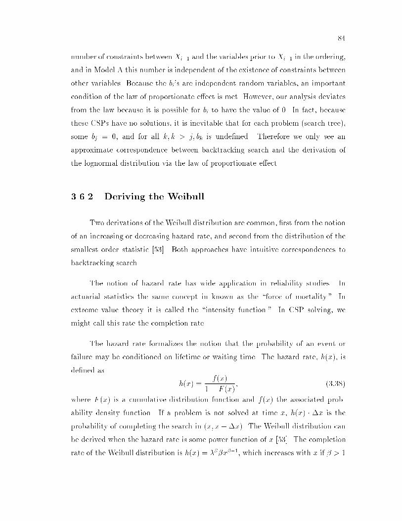
84

number of constraints betweenXi�1 and the variables prior to Xi�1 in the ordering,

and in Model A this number is independent of the existence of constraints between

other variables. Because the bi's are independent random variables, an important

condition of the law of proportionate e�ect is met. However, our analysis deviates

from the law because it is possible for bi to have the value of 0. In fact, because

these CSPs have no solutions, it is inevitable that for each problem (search tree),

some bj = 0, and for all k; k > j; bk is unde�ned. Therefore we only see an

approximate correspondence between backtracking search and the derivation of

the lognormal distribution via the law of proportionate e�ect.

3.6.2 Deriving the Weibull

Two derivations of the Weibull distribution are common, �rst from the notion

of an increasing or decreasing hazard rate, and second from the distribution of the

smallest order statistic [53]. Both approaches have intuitive correspondences to

backtracking search.

The notion of hazard rate has wide application in reliability studies. In

actuarial statistics the same concept in known as the \force of mortality." In

extreme value theory it is called the \intensity function." In CSP solving, we

might call this rate the completion rate.

The hazard rate formalizes the notion that the probability of an event or

failure may be conditioned on lifetime or waiting time. The hazard rate, h(x), is

de�ned as

h(x) =f(x)

1 � F (x); (3:38)

where F (x) is a cumulative distribution function and f(x) the associated prob-

ability density function. If a problem is not solved at time x, h(x) � �x is the

probability of completing the search in (x; x+�x). The Weibull distribution can

be derived when the hazard rate is some power function of x [53]. The completion

rate of the Weibull distribution is h(x) = ���x��1, which increases with x if � > 1

85

and decreases with x for � < 1. For the exponential distribution, a special case of

the Weibull distribution with � = 1, h(x) = � is constant. Thus when � < 1, each

node in the search tree has a smaller probability of being the last one than the one

before it. In backtracking search on solvable problems, the e�ort required to �nd

a solution is strongly in uenced by the number of solutions and their distribution

in the search space. As search continues without completion, the probability that

there are many solutions decreases. This in turn increases the probability that the

search will take a relatively large amount of e�ort. The decreasing completion rate

of the Weibull distribution re ects the observation that easy solvable problems

often have many solutions, and not �nding a solution early in the search increases

the estimate of how long the search will take.

The Weibull distribution can also be derived from the study of the smallest

extreme. Let (X1;X2; . . . ;Xn) be a random sample of n observations from dis-

tribution F . It is possible to compute the distribution of the minimum value in

(X1;X2; . . . ;Xn), called the �rst order statistic, as a function of F and n. For

several types of function F , and as n becomes large, the distribution of the �rst

order statistic is a Weibull distribution. In particular, the distribution of the �rst

order statistic from a Weibull distribution is also a Weibull distribution.

Consider a backtracking search strategy in which all the subtrees rooted at

level r in the search tree are searched in parallel. For instance, if r = 4 and D (the

number of values per variable) = 3, then there are 34 such subtrees, although some

subtrees may not exist because of dead-ends before level 4. Let Si be the amount

of work (e.g. search space or consistency checks) expended on the i'th subtree.

If the problem has a solution, let S0 be the amount of e�ort devoted to search in

the �rst subtree which produces a solution. Then the total e�ort required (over

all subtrees and over all processors) will be approximately Dr �S0, less some time

not spent on subtrees which �nish without a solution after less than S0 work. If we

can approximate the distribution of �nding a solution in a subtree with a Weibull

86

distribution, then the distribution over the entire tree may also have a Weibull

distribution.

3.7 Related Work

The primary factor which distinguishes our work from similar studies is that

we focus not only on the expected e�ort required to solve CSPs, but also on the

variance and distribution.

Haralick and Elliott [40] show how to compute the expected number of nodes

and consistency checks for backtracking and forward checking, based on a model

of random CSP similar to Model A.

Nudel [65] works with a model of CSP distribution in which instances are

randomly chosen from the set of all problems that have a speci�ed number of

compatible value pairs, Iij, for every pair of variables Xi and Xj .

Mitchell ([57]) shows results from a set of experiments in which the run time

mean, standard deviation, and maximum value all increase as more and more

samples are recorded. The �nding is similar to that in Fig. 3.2, and is entirely

consistent with the Weibull and lognormal distributions, as both tend to have long

tails and high variance. Hogg and Williams ([41]) provide an analytical analysis

of the exponentially long tail of CSP hardness distributions. Their work suggests

that the distributions at the 50% satis�able point are quite di�erent than the

distributions elsewhere in the parameter space. Selman and Kirkpatrick ([77])

have noted and analyzed the di�ering distributions of satis�able and unsatis�able

instances. Kwan ([49]) has recently shown empirical evidence that the hardness of

randomly generated CSPs and 3-coloring problems is not distributed normally.

87

3.8 Concluding remarks

More accurate summarization of experimental results was our initial motiva-

tion for investigating the distribution of CSP hardness. It remains primary, but

several other bene�ts of this study are also worth highlighting. Well-developed sta-

tistical techniques, based on the assumption of a known underlying distribution,

are available for estimating parameters based on data that have been \censored"

above a certain point [64]. This may aid the interpretation of an experiment in

which runs are terminated after a certain time point. In certain cases, it may be

advantageous to design an experiment with a time-bound, knowing that the loss

of accuracy in estimating the parameters of the distribution due to not having any

data from the right tail is more than compensated for by the increased number of

instances that can be run to completion.

Knowing the distribution will also enable a more precise comparison of com-

peting algorithms. For instance, it is easier to determine whether the di�erence

in the means of two experiments is statistically signi�cant if the population distri-

butions are known. Knowing that the distribution is not normal will prevent the

researcher from relying on a statistical test that makes an assumption of normality.

Knowledge of the distribution function can be used in resource-limited sit-

uations to suggest an optimum time-bound for an algorithm to process a single

instance. Examples would be running multiple algorithms on a single instance in

a time-sliced manner, as proposed in [42], and environments where the goal is to

complete as many problems as possible in a �xed time period.

The most important direction in which this line of research can be pursued

is to determine whether the distribution of work required to solve real-world CSPs

can also be usefully approximated by simple continuous distributions, perhaps the

lognormal and theWeibull, or perhaps other distribution functions. In applications

such as scheduling there are usually a large number of CSPs to solve which can

88

be thought of as coming from an (unknown) distribution. The distribution of

solving-time for these problems may also display useful regularities.

Chapter 4

Backjumping and Dynamic

Variable Ordering

4.1 Overview of Chapter

We propose an algorithm, dubbed BJ+DVO, which combines con ict-based

backjumping and a dynamic variable ordering heuristic which incorporates forward

checking style �ltering of future domains1. Experimental evaluation shows that

BJ+DVO is e�ective on random problem instances created with a wide range of

parameters.

4.2 Introduction

In Chapter 2 we discussed two standard constraint satisfaction algorithms,

con ict-based backjumping (BJ) and forward checking (FC). Although the two

algorithms are both based on backtracking, they take quite di�erent approaches

to identifying and rejecting instantiations which con ict with a constraint. In

this chapter we develop an algorithm that combines backjumping with a dynamic

variable ordering heuristic which is based on information acquired by a forward

checking style processing of future variables.

1BJ+DVO was �rst described and evaluated in Frost and Dechter [27].

89

90

Backjumping can be termed a \look-back" algorithm. Like backtracking,

backjumping rejects a potential value for a variable if it is incompatible with the

current set of instantiated variables. Backjumping goes beyond backtracking in

sophistication because it is able to jump back over variables that are not responsible

for a dead-end.

Forward checking uses a \look-ahead" approach. After a value v is assigned

to a variable X, all values in the domains of future variables that are incompatible

with X = v are removed while X = v. Forward checking does not need to test

whether a value in the domain of the current variable is compatible with the

previous partial instantiation, since incompatible values were temporarily �ltered

out when the earlier variables were assigned values.

Because backjumping and forward checking use two orthogonal methods for

improving CSP search, it is natural to wonder whether it makes sense to combine

the two approaches. Worst-case analyses such as that of Kondrak and van Beek

[47] o�er no answer, since we do not expect a combination algorithm to have better

worst-case performance.

Prosser [68] performed a small experimental study, limited to random per-

mutations of a single problem, with several algorithms including \BJ+FC", which

combines backjumping and forward checking but uses a �xed variable ordering.

The new element in algorithm BJ+DVO is that it combines, in e�ect, BJ+FC

with dynamic variable ordering. In addition, we present an extensive and sys-

tematic evaluation on large instances, which was not done before. Our empirical

evidence demonstrates that the combination of backjumping, forward checking,

and dynamic variable ordering is indeed a strong performer on a wide variety of

CSPs.

91

Backjumping with DVO0. (Initialize.) Set D0

i Di for 1 � i � n. Set Pi ; for 1 � i � n.

1. (Step forward.) If Xcur is the last variable, then all variables have valueassignments; exit with this solution. Otherwise, set cur equal to theindex of the next variable, selected according to avariable-ordering-heuristic (see Fig. 4.2). Set Pcur ;.

2. Select a value x 2 D0cur. Do this as follows:

(a) If D0cur = ;, go to 3.

(b) Pop x from D0cur and instantiate Xcur x.

(c) Examine the future variables Xi; cur < i � n. For each v in D0i, if

Xi = v con icts with ~xcur then remove v from D0i and add Xcur to

Pi; if D0i becomes empty, go to (d) (without examining other Xi's).

(d) Go to 1.

3. (Backjump.) If Pcur = ; (there is no previous variable), exit with\inconsistent." Otherwise, set P Pcur; set cur equal to the index ofthe last variable in P . Set Pcur Pcur [ P �fXcurg. Reset all D0 sets tothe way they were before Xcur was last instantiated. Go to 2.

Figure 4.1: The BJ+DVO algorithm.

4.3 The BJ+DVO Algorithm

This chapter reports an algorithm which is designed to combine the desirable

features of backjumping, forward checking, and dynamic variable ordering. We

call this combination BJ+DVO, and it is described in Fig. 4.1.

Step 1 of BJ+DVO utilizes a variable ordering heuristic, which selects an

uninstantiated variable to be the next in the ordering. The variable ordering

heuristic we use is described in Fig. 4.2 and is discussed below.

Step 2 of BJ+DVO is patterned after the forward checking algorithm in

Section 2.8, with two changes. The �rst change is that con icts are recorded

using parent sets Pi. The parent sets have the same function as in backjumping:

Pi is a set of variables Xk, each of which is the last in a partial instantiation

92

~xk which con icts with some value of Xi. The presence of a forward checking

style look-ahead mechanism a�ects how the P 's are updated. In backjumping,

earlier variables are added to Pcur . In BJ+DVO, Xcur is added to the parent

set of a future variable. This re ects the fact that pure look-back algorithms

(such as backjumping) compare the current variable with earlier variables, while

an algorithm having a look-ahead component, such as BJ+DVO, removes values

from the domains of future variables.

The other change to step 2 marks a departure from all the earlier algorithms

in Chapter 2. In the earlier algorithms, if a value x fromD0cur was found incompat-

ible, either by a look back or a look forward check with other variables, there was

a \go to (a)" step which continued the search with the next value of the current

variable. In contrast, BJ+DVO's step 2 always proceeds to step 1 after assigning

a value to Xcur. If that value causes the domain of a future variable Xe to become

empty, then the variable ordering heuristic will select Xe to be the next variable,

and after step 2 (a) (for Xe with an empty domain) is executed, control will go

the backjump step, step 3. The backjump from Xe will of course be a step back to

the immediately preceeding variable, since it was the instantiation of that variable

which caused Xe to have an empty domain. Thus in BJ+DVO, a backjump from

a leaf dead-end is always to the immediately preceeding variable. The fact that

selecting to be next a variable with an empty domain makes Gaschnig's backjump-

ing { that is, backjumping from leaves in the search tree { redundant was noted

in [3] and [47].

In step 2 (b), the values of each variable are considered in an arbitrary but

�xed order.

Step 3 of BJ+DVO is identical to the step 3 of the backjumping algorithm

from chapter 2, section 6. The most recent variable in the Pcur set is identi�ed, and

that variable becomes current, with its parent set being merged with the parent

set of the dead-end variable.

93

VARIABLE-ORDING-HEURISTIC1. If no variable have yet been selected, select the variable that participates

in the most constraints. In case of a tie, select one variable arbitrarily.

2. Let m be the size of the smallest D0 set of a future variable.

(a) If there is one future variable with D0 size = m, then select it.

(b) If there is more than one, select the one that participates in the mostconstraints (in the original problem), breaking any remaining tiesarbitrarily.

Figure 4.2: The variable ordering heuristic used by BJ+DVO.

The main idea of the variable ordering heuristic, described in Fig. 4.2, is

to select the future variable with the smallest remaining domain. As noted in

Chapter 2, this idea was proposed by Haralick and Elliot [40] under the rubric

\fail �rst." We have found that augmenting the fail-�rst strategy with the tie-

breaking rules described in step 1 and step 2 (b) of Fig. 4.2 produces a 10% to

30% improvement in performance, when compared to BJ+DVO without the tie-

breakers (data not shown). The guiding intuition behind the tie-breakers is to

select the variable that is the most constraining, and thus most likely to reduce

the size of the D0 sets of those variables selected after it.

4.4 Experimental Evaluation

The goal of the experiments was to determine whether combining backjump-

ing, forward-checking style look-ahead, and dynamic variable ordering into a single

procedure would be an e�ective combination. Six algorithms or combination al-

gorithms were employed: BT+MW (simple backtracking with the min-width vari-

able ordering heuristic), BJ+MW (con ict-directed backjumping with min-width),

FC+MW (forward checking with min-width), BJ+FC+MW (backjumping with

forward checking and min-width), BT+DVO (backtracking with dynamic variable

94

ordering), and BJ+DVO (backjumping with dynamic variable ordering). We se-

lected a variety of parameters for the random problem generator, and for each set of

parameters generated 2,000 problem instances. The experiments show the relative

performance of the six algorithms over a range of values for D, T , and C, and for

increasing N . For selected value of D and T , we generated instances with several

values of N and C. Because the parameters are all near the cross-over point, there

are about 1,000 solvable and unsolvable instances for each set. Tables 4.1, 4.2, 4.3,

and 4.4 report mean CPU seconds (on a SparcStation 4, 110 MHz processor) for

each experiment, with unsolvable and solvable problems reported separately. CPU

seconds are rounded to two decimal points; reported values of \0.00" indicate that

the average was less than 0.005. A position in the tables is in parentheses when the

experiment was stopped part way through; \n.r." indicates that the experiment

was not run.

For convenience, experiments with D = 3 are reported in Table 4.1 and

4.2, while experiments with D = 6 are summarized in Table 4.3 and 4.4. Within

each table, sets of experiments with di�erent values of parameter T are divided by

horizontal lines.

The �rst four columns of Tables 4.1 through 4.4 show the results of us-

ing algorithms which have a �xed variable ordering. In all cases the combination

BT+FC+MW performed best, and simple backtracking, BT+MW, least well. The

relative performance of BJ+MW and FC+MW depended on the domain size pa-

rameter D. On problems with D=3, BJ+MW solved problems using less CPU

time and FC+MW, while FC+MW was better with D=6.

The experiments in general support the conclusion that the BJ+DVO com-

bination is an extremely e�ective one. Its only serious rival, among the algorithms

we tested, is BT+DVO when parameter T is relatively small, that is, when the

constraints are loose. With D=3 and T=:111, BJ+DVO is marginally worse than

BT+DVO on unsolvable problems, and marginally better on solvable problems

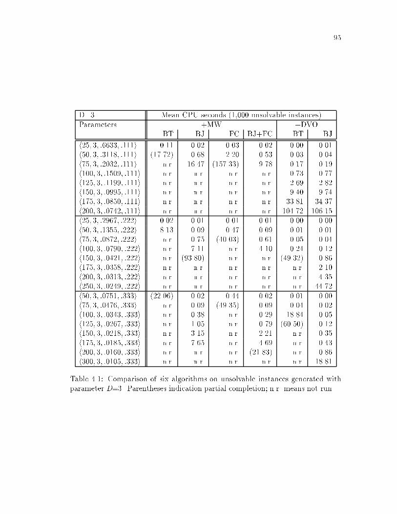
95

D=3 Mean CPU seconds (1,000 unsolvable instances)Parameters +MW +DVO

BT BJ FC BJ+FC BT BJ

h25; 3; :6633; :111i 0.11 0.02 0.03 0.02 0.00 0.01h50; 3; :3118; :111i (17.72) 0.68 2.20 0.53 0.03 0.04h75; 3; :2032; :111i n.r. 16.47 (157.33) 9.78 0.17 0.19h100; 3; :1509; :111i n.r. n.r. n.r. n.r. 0.73 0.77h125; 3; :1199; :111i n.r. n.r. n.r. n.r. 2.69 2.82h150; 3; :0995; :111i n.r. n.r. n.r. n.r. 9.40 9.74h175; 3; :0850; :111i n.r. n.r. n.r. n.r. 33.81 34.37h200; 3; :0742; :111i n.r. n.r. n.r. n.r. 104.72 106.15h25; 3; :2967; :222i 0.02 0.01 0.01 0.01 0.00 0.00h50; 3; :1355; :222i 8.13 0.09 0.47 0.09 0.01 0.01h75; 3; :0872; :222i n.r. 0.75 (40.03) 0.61 0.05 0.04h100; 3; :0790; :222i n.r. 7.11 n.r. 4.10 0.24 0.12h150; 3; :0421; :222i n.r. (93.80) n.r. n.r. (49.32) 0.86h175; 3; :0358; :222i n.r. n.r. n.r. n.r. n.r. 2.10h200; 3; :0313; :222i n.r. n.r. n.r. n.r. n.r. 4.35h250; 3; :0249; :222i n.r. n.r. n.r. n.r. n.r. 44.72h50; 3; :0751; :333i (22.06) 0.02 0.44 0.02 0.01 0.00h75; 3; :0476; :333i n.r. 0.09 (49.35) 0.09 0.04 0.02h100; 3; :0343; :333i n.r. 0.38 n.r. 0.29 18.84 0.05h125; 3; :0267; :333i n.r. 1.05 n.r. 0.79 (60.50) 0.12h150; 3; :0218; :333i n.r. 3.15 n.r. 2.21 n.r. 0.35h175; 3; :0185; :333i n.r. 7.65 n.r. 4.69 n.r. 0.43h200; 3; :0160; :333i n.r. n.r. n.r. (21.83) n.r. 0.86h300; 3; :0105; :333i n.r. n.r. n.r. n.r. n.r. 18.81

Table 4.1: Comparison of six algorithms on unsolvable instances generated withparameter D=3. Parentheses indication partial completion; n.r. means not run.

96

D=3 Mean CPU seconds (1,000 solvable instances)Parameters +MW +DVO

BT BJ FC BJ+FC BT BJ

h25; 3; :6633; :111i 0.05 0.01 0.02 0.01 0.00 0.00h50; 3; :3118; :111i (9.08) 0.33 1.43 0.26 0.02 0.02h75; 3; :2032; :111i n.r. 8.20 (129.87) 5.40 0.09 0.09h100; 3; :1509; :111i n.r. n.r. n.r. n.r. 0.33 0.35h125; 3; :1199; :111i n.r. n.r. n.r. n.r. 1.22 1.26h150; 3; :0995; :111i n.r. n.r. n.r. n.r. 4.34 4.42h175; 3; :0850; :111i n.r. n.r. n.r. n.r. 15.99 15.91h200; 3; :0742; :111i n.r. n.r. n.r. n.r. 46.29 45.32h25; 3; :2967; :222i 0.01 0.00 0.00 0.01 0.00 0.00h50; 3; :1355; :222i 6.26 0.05 0.39 0.05 0.01 0.01h75; 3; :0872; :222i n.r. 0.41 31.76 0.34 0.03 0.03h100; 3; :0790; :222i n.r. 3.83 (482.79) n.r. 0.32 0.08h150; 3; :0421; :222i n.r. (58.75) n.r. n.r. 13.28 0.68h175; 3; :0358; :222i n.r. n.r. n.r. n.r. 25.67 1.37h200; 3; :0313; :222i n.r. n.r. n.r. n.r. (38.14) 3.44h250; 3; :0249; :222i n.r. n.r. n.r. n.r. n.r. 32.01h50; 3; :0751; :333i (9.46) 0.01 0.29 0.02 0.01 0.01h75; 3; :0476; :333i n.r. 0.06 (32.07) 0.07 0.03 0.01h100; 3; :0343; :333i n.r. 0.17 n.r. 0.18 0.26 0.03h125; 3; :0267; :333i n.r. 0.54 n.r. 0.50 (16.91) 0.05h150; 3; :0218; :333i n.r. 1.21 n.r. 1.07 n.r. 0.11h175; 3; :0185; :333i n.r. 4.17 n.r. 2.29 n.r. 0.17h200; 3; :0160; :333i n.r. n.r. n.r. (6.38) n.r. 0.28h300; 3; :0105; :333i n.r. n.r. n.r. n.r. n.r. 7.14

Table 4.2: Comparison of six algorithms on solvable instances generated withparameter D=3. Parentheses indication partial completion; n.r. means not run.

97

D=6 Mean CPU seconds (1,000 unsolvable instances)Parameters +MW +DVO

BT BJ FC BJ+FC BT BJ

h35; 6; :8420; :111i (1,189) (167.00) (52.18) 42.12 1.34 1.46h40; 6; :7308; :111i n.r. n.r. n.r. n.r. 3.17 3.45h50; 6; :5796; :111i n.r. n.r. n.r. n.r. 16.00 17.56h60; 6; :4797; :111i n.r. n.r. n.r. n.r. 81.07 88.22h25; 6; :5533; :222i 1.44 0.44 0.31 0.29 0.05 0.06h40; 6; :3346; :222i (61.78) 13.87 8.78 6.38 0.51 0.56h50; 6; :2653; :222i n.r. n.r. 75.05 45.00 2.00 2.20h60; 6; :2192; :222i n.r. n.r. n.r. n.r. 7.53 8.17h75; 6; :1744; :222i n.r. n.r. n.r. n.r. 54.71 58.92h25; 6; :3333; :333i 0.30 0.10 0.08 0.08 0.02 0.02h40; 6; :2000; :333i (103.66) 1.75 1.28 0.91 0.14 0.15h50; 6; :1576; :333i n.r. n.r. 7.11 4.10 0.44 0.46h75; 6; :1038; :333i n.r. n.r. n.r. (32.38) 6.77 6.85h100; 6; :0772; :333i n.r. n.r. n.r. n.r. (91.47) 85.96h25; 6; :2200; :444i 0.09 0.03 0.03 0.03 0.01 0.01h50; 6; :1029; :444i (10.70) 1.44 1.10 0.57 0.15 0.13h60; 6; :0847; :444i n.r. 5.35 4.55 1.81 0.41 0.33h75; 6; :0670; :444i n.r. n.r. n.r. 10.48 1.67 1.17h100; 6; :0497; :444i n.r. n.r. n.r. n.r. 21.19 10.18h50; 6; :0678; :555i (9.36) 0.42 0.19 0.18 0.14 0.04h75; 6; :0432; :555i n.r. 3.41 2.54 2.01 49.06 0.32h100; 6; :0319; :555i n.r. (46.21) 32.27 17.83 n.r. 5.59

Table 4.3: Comparison of six algorithms on unsolvable instances generated withparameter D=6. Parentheses indication partial completion; n.r. means not run.

98

D=6 Mean CPU seconds (1,000 solvable instances)Parameters +MW +DVO

BT BJ FC BJ+FC BT BJ

h35; 6; :8420; :111i (498.72) (68.07) (23.17) 17.23 0.58 0.63h40; 6; :7308; :111i n.r. n.r. n.r. n.r. 1.25 1.36h50; 6; :5796; :111i n.r. n.r. n.r. n.r. 6.67 7.31h60; 6; :4797; :111i n.r. n.r. n.r. n.r. 33.92 36.88h25; 6; :5533; :222i 0.69 0.20 0.15 0.14 0.03 0.03h40; 6; :3346; :222i (19.40) 7.40 4.85 3.36 0.25 0.27h50; 6; :2653; :222i n.r. n.r. 40.55 23.10 0.96 1.05h60; 6; :2192; :222i n.r. n.r. n.r. n.r. 3.75 4.05h75; 6; :1744; :222i n.r. n.r. n.r. n.r. 27.81 29.87h25; 6; :3333; :333i 0.17 0.05 0.05 0.04 0.01 0.01h40; 6; :2000; :333i (41.48) 1.06 0.87 0.58 0.08 0.09h50; 6; :1576; :333i n.r. n.r. 5.11 2.62 0.25 0.27h75; 6; :1038; :333i n.r. n.r. n.r. (12.56) 4.19 4.18h100; 6; :0772; :333i n.r. n.r. n.r. n.r. (61.99) 57.51h25; 6; :2200; :444i 0.06 0.02 0.02 0.02 0.01 0.01h50; 6; :1029; :444i n.r. 1.20 1.25 0.49 0.11 0.09h60; 6; :0847; :444i n.r. 4.56 8.96 1.78 0.33 0.25h75; 6; :0670; :444i n.r. n.r. n.r. 7.99 1.99 1.15h100; 6; :0497; :444i n.r. n.r. n.r. n.r. 23.36 7.91h50; 6; :0678; :555i (14.30) 0.31 0.18 0.16 0.12 0.04h75; 6; :0432; :555i n.r. 1.75 1.86 1.79 165.19 0.28h100; 6; :0319; :555i n.r. (31.08) 39.47 13.29 n.r. 2.08

Table 4.4: Comparison of six algorithms on solvable instances generated withparameter D=6. Parentheses indication partial completion; n.r. means not run.

99

(see Table 4.1 and Table 4.2). When T is greater than .111, BJ+DVO substan-

tially outperforms BT+DVO. With D=6, the dividing line is near T = :333. At

this and smaller values of T , BJ+DVO underperforms BT+DVO, although by no

more, on average, than 10%. When D=6 and T is greater than .333, BJ+DVO is

substantially better than BT+DVO.

CPU seconds is the basis for comparing algorithms in Tables 4.1{4.4. Tables

4.5 and 4.6 are based on the same experiments as the earlier tables, but show mean

consistency checks and mean nodes in search space for selected sets of parameters

and for the algorithms BT+DVO and BJ+DVO only. In several cases where

BJ+DVO requires more CPU time, on average, than BT+DVO, it makes fewer

consistency checks and expands a slightly smaller search space. For instance, in

the experiment with parameters h150; 3; :0995; :111i and unsolvable problems (see

the �rst line in Table 4.5), BT+DVO makes 7% more consistency checks than

BJ+DVO (1,048,156 compared to 981,043) and searches 7% more nodes (37,171

compared to 34,674), yet on average requires only 97% as much CPU time. This

pattern holds not only for the average, but also on an instance by instance basis.

Over three fourths of the unsolvable problems with these parameters made between

1% and 15% more consistency checks with BT+DVO than with BJ+DVO, but

�nished in 85% to 99% as much CPU time.

On large problems (N=175 and N=200) generated with D=3 and T=:111,

BJ+DVO is slightly worse than BT+DVO on unsolvable problems and slightly bet-

ter than BT+DVO on solvable problems (when measuring CPU time). Unsolvable

branches of solvable problems tend to be somewhat deeper than the average branch

of an unsolvable problem with the same parameters. Thus solvable problems fre-

quently have deeper search trees that unsolvable problems, and the more time the

search spends deep in the search tree, the more opportunity exists for backjumping

to be useful.

It can be interesting to examine not only the mean performance of algorithms,

but the entire distribution of computational e�ort over a set of problem instances.

100

Mean values (1,000 unsolvable instances)

Parameters BT+DVO BJ+DVOCC Nodes CPU CC Nodes CPU

h150; 3; :0995; :111i 1,058,173 37,484 9.40 991,163 35,003 9.74h175; 3; :0850; :111i 3,095,396 109,124 33.81 2,873,370 100,981 34.37h200; 3; :0742; :111i 8,735,964 306,628 104.72 8,043,054 281,559 106.15

h100; 3; :0790; :222i 11,007 1,002 0.24 8,775 679 0.12h150; 3; :0421; :222i 570,635 189,997 49.32 38,856 3,099 0.86h175; 3; :0358; :222i 81,473 6,697 2.10h200; 3; :0313; :222i 150,959 12,346 4.53

h100; 3; :0343; :333i 542,233 129,338 18.84 1,943 257 0.05h125; 3; :0267; :333i 955,740 294,718 60.50 3,800 524 0.12h150; 3; :0218; :333i 8,602 1,293 0.35h200; 3; :0160; :333i 32,763 7,353 2.00

h50; 6; :5796; :111i 7,677,173 130,284 16.00 7,615,125 129,061 17.56h60; 6; :4797; :111i 33,521,936 562,191 81.07 33,154,152 555,195 88.22

Table 4.5: Comparison of BT+DVO and BJ+DVO on unsolvable problems, mea-suring consistency checks, nodes in the search space, and CPU seconds.

Mean values (1,000 solvable instances)

Parameters BT+DVO BJ+DVOCC Nodes CPU CC Nodes CPU

h150; 3; :0995; :111i 477,156 17,808 4.34 441,225 16,387 4.42h175; 3; :0850; :111i 1,425,292 52,737 15.99 1,300,459 47,932 15.91h200; 3; :0742; :111i 3,786,347 138,251 46.29 3,378,094 122,824 45.32

h100; 3; :0790; :222i 10,253 1,744 0.32 5,267 488 0.08h150; 3; :0421; :222i 214,932 48,817 13.28 28,526 2,740 0.68h175; 3; :0358; :222i 346,607 79,455 25.67 48,208 4,368 1.37h200; 3; :0313; :222i 112,886 10,309 3.63

h100; 3; :0343; :333i 6,882 1,745 0.26 1,609 276 0.05h125; 3; :0267; :333i 279,194 79,311 16.91 1,609 276 0.05h150; 3; :0218; :333i 2,727 449 0.11h200; 3; :0160; :333i 40,426 7,148 2.29

h50; 6; :5796; :111i 3,171,321 54,924 6.67 3,143,167 54,353 7.31h60; 6; :4797; :111i 13,908,893 237,554 33.92 13,745,036 234,363 36.88

Table 4.6: Comparison of BT+DVO and BJ+DVO on solvable problems, measur-ing consistency checks, nodes in the search space, and CPU seconds.

101

Taking advantage of the results from Chapter 3, we estimate the parameters of the

lognormal distributions that most closely approximate the empirical distributions

on unsolvable instances generated with h100; 3; 0:0343; 0:333i and searched by al-

gorithms BJ+MW, BJ+FC+MW, BT+DVO, and BJ+DVO. In Fig. 4.3 we graph

the lognormal distributions, measuring both the number of consistency checks

made (top chart) and the number of CPU seconds required (bottom chart). The

estimated � and � parameters are speci�ed inside the chart. Comparing the re-

sulting curves, we see that BT+DVO and BJ+DVO solve the most problems with

a small amount of e�ort { the distributions for these two algorithms have high

modes far to the left. However, BT+DVO required a very large amount of e�ort

on a few instances. The mean CPU time and consistency checks for BT+DVO is

therefore higher than for the other algorithms, and its � parameter is the highest,

indicating a heavy right tail and a relatively large number of hard instances.

102

h100; 3; 0:0343; 0:333iBJ+MW: �=9:55 �=1:42BJ+FC+MW: �=8:38 �=1:35BT+DVO: �=7:31 �=1:67BJ+DVO: �=6:89 �=1:10

0 2,500 10,000 17,500Consistency Checks

Frequency

.02

.04

.06

BJ+MW

BJ+FC+MW

BT+DVO

BJ+DVO

h100; 3; 0:0343; 0:333iBJ+MW: �=�1:83 �=1:15BJ+FC+MW: �=�2:02 �=1:11BT+DVO: �=�2:27 �=1:52BJ+DVO: �=�2:63 �=0:98

0 0.0625 0.2500 0.4375CPU Seconds

Frequency

.01

.02

BJ+MW

BJ+FC+MW

BT+DVO

BJ+DVO

Figure 4.3: Lognormal curves based on unsolvable problems generated from pa-rameters h100; 3; 0:0343; 0:333i. The top chart is based on consistency checks, thebottom chart on CPU seconds. � and � parameters were estimated using theMaximum Likelihood Estimator (see Chapter 3).

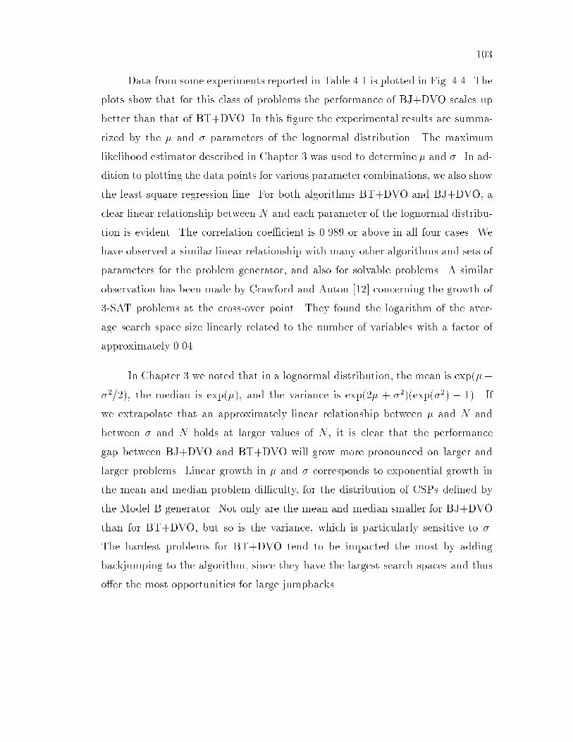
103

Data from some experiments reported in Table 4.1 is plotted in Fig. 4.4. The

plots show that for this class of problems the performance of BJ+DVO scales up

better than that of BT+DVO. In this �gure the experimental results are summa-

rized by the � and � parameters of the lognormal distribution. The maximum

likelihood estimator described in Chapter 3 was used to determine � and �. In ad-

dition to plotting the data points for various parameter combinations, we also show

the least square regression line. For both algorithms BT+DVO and BJ+DVO, a

clear linear relationship between N and each parameter of the lognormal distribu-

tion is evident. The correlation coe�cient is 0.989 or above in all four cases. We

have observed a similar linear relationship with many other algorithms and sets of

parameters for the problem generator, and also for solvable problems. A similar

observation has been made by Crawford and Auton [12] concerning the growth of

3-SAT problems at the cross-over point. They found the logarithm of the aver-

age search space size linearly related to the number of variables with a factor of

approximately 0.04.

In Chapter 3 we noted that in a lognormal distribution, the mean is exp(�+

�2=2), the median is exp(�), and the variance is exp(2� + �2)(exp(�2) � 1). If

we extrapolate that an approximately linear relationship between � and N and

between � and N holds at larger values of N , it is clear that the performance

gap between BJ+DVO and BT+DVO will grow more pronounced on larger and

larger problems. Linear growth in � and � corresponds to exponential growth in

the mean and median problem di�culty, for the distribution of CSPs de�ned by

the Model B generator. Not only are the mean and median smaller for BJ+DVO

than for BT+DVO, but so is the variance, which is particularly sensitive to �.

The hardest problems for BT+DVO tend to be impacted the most by adding

backjumping to the algorithm, since they have the largest search spaces and thus

o�er the most opportunities for large jumpbacks.

104

� � BJ+DVO? � BT+DVO� � BJ+DVO� � BT+DVO

25 50 100 150 200N

3

5

7

9

11

13

�

�

��

�

�� �

0:0281N + 3:1496

?

?

?

?

?

?

0:0322N + 3:0087

.5

1.0

1.5

2.0

��

� � �� �

� 0:0049N + :3976

��

��

� �0:0085N + :2390

Figure 4.4: Data on search space size of unsolvable problems in experiments withparameters D=3, T=:222, and varying values of N and C (as in Table 4.1), usingalgorithms BT+DVO and BJ+DVO. Points represent estimated � (left hand scale)and � (right hand scale) for each algorithm, assuming a lognormal distribution.Lines (solid for BJ+DVO, dotted for BT+DVO) show best linear �t. The formulato the right of each line shows the slope and the y-axis intercept.

105

Mean CPU seconds Mean Mean per 10,000Parameters BT+DVO BJ+DVO EJ ratio EJ � 5 EJ � 10h175; 3; :0850; :111i 33.81 34.37 0.61 225 54h175; 3; :0358; :222i 325.77 2.30 0.80 391 132h175; 3; :0185; :333i 0.43 1.16 651 271h50; 6; :5796; :111i 15.74 17.30 0.15 6 0h60; 6; :2192; :222i 7.60 12.41 0.19 13 0h75; 6; :1038; :333i 5.96 6.05 0.25 31 2h100; 6; :0497; :444i 21.19 10.18 0.39 94 15h100; 6; :0319; :555i 5.59 0.56 215 70

Table 4.7: Extract of data from Table 4.1 and Table 4.3, plus record of extra jumpsmade by backjumping. Unsolvable instances only.

4.5 Discussion

Why does the relative performance of BT+DVO and BJ+DVO seem to de-

pend on the tightness of the constraints? The answer lies in the costs and bene�ts

of backjumping. The overhead of backjumping, primarily maintaining and check-

ing the Pi sets, does not seem to pay o�, on average, on problems with relatively

loose constraints. With tighter constraints, the average size of the parent set tends

to shrink, because it is more likely that a single variable in the parent set is in con-

ict with multiple values of the dead-end variable. A smaller parent set increases

the likelihood that backjumping will skip over a large number of variables in its

jump. To assess this explanation quantitatively, we can examine more closely the

behavior of backjumping.

During the execution of the BJ+DVO algorithm measurements were made

pertaining to the e�ectiveness of backjumping; they are reported in Table 4.7. The

measurements were made during a second, instrumented, run of the algorithm, so

that the CPU times cited in the tables would not be a�ected by the overhead of

recording additional information. Our goal was to discover how much jumping

BJ+DVO was doing. We recorded, for each problem instance, the total number

of \extra jumps" made, de�ning an extra jump as returning to a variable other

106

than the immediately preceeding one. For instance, if after a dead-end at X20

the highest variable in P20 (the parent set of X20) is X17, this counts as 2 extra

jumps. Dividing the total number of extra jumps by the number of interior dead-

ends yields the \extra jump ratio" for an instance; the average for each set of

parameters is reported in the \EJ ratio" column of Table 4.7. Leaf dead-ends were

excluded from this calculation because, as discussed in section 4.3, the backjump

from a leaf dead-end is always a single step to the immediately preceeding variable

(no extra jumps) when DVO is in e�ect. The last two columns of Table 4.7 show

the average number of large backjumps, size �ve or greater and size ten or greater,

per 10,000 interior dead-ends.

It is not surprising to observe in Table 4.7 that as T increases and BJ+DVO

becomes more e�ective than BT+DVO, the quantity of extra jumps increases.

It is perhaps surprising to see how large an impact a seemingly small number

of extra jumps can make. For instance, in the set of problems with parame-

ters h175; 3; :0358; :222i BJ+DVO requires half a percent as much CPU time as

does BT+DVO, the result of jumping back on average slightly less than one ex-

tra variable per interior dead-end. In this particular set of unsolvable problems,

one instance required 23.6 CPU hours with BT+DVO and only 2 CPU seconds

with BJ+DVO (excluding this problem instance, the means would be 26.17 CPU

seconds under BT+DVO and an unchanged 2.10 CPU seconds under BJ+DVO).

BJ+DVO made 3,076 extra jumps on this instance and had 2,523 interior dead-

ends, for an extra jump ratio of 1.22, somewhat higher than average. On this

instance BJ+DVO once jumped over 88 variables, and had 59 jumps of 10 or more

variables.

The combination of DVO and backjumping is particularly felicitous because

of the complementary strengths of the backjumping and dynamic variable ordering

components. Backjumping is more e�ective on sparser constraint graphs (low value

of parameter C), since the average size of each \jump" tends to increase with

increasing sparseness. The dynamic variable ordering heuristic, in contrast, tends

107

Parameters single value domainh75; 3; :2032; :111i 92.8%h75; 3; :0872; :222i 78.9%h75; 3; :0476; :333i 70.9%h40; 6; :3346; :222i 80.2%h40; 6; :2000; :333i 77.1%h40; 6; :1308; :444i 72.4%

Table 4.8: Data on unsolvable problems with N=75;D=3 (�rst three lines), drawnfrom the same experiments as in Table 4.1, and data with N=40;D=6 (secondthree lines), drawn from the same experiments as in Table 4.3. The algorithm isBT+DVO, and the \single value domain" column reports the frequency in non-dead-end situations that there was a future variable with exactly one value in itsdomain.

to function better when there are many constraints (high value of parameter C),

since each constraint provides information it can utilize in deciding on the next

variable. We assessed this observation quantitatively by recording the performance

of BT+DVO over a variety of values of C, while holding the number of variables

N and the domain size D constant. Speci�cally, we measured the frequency with

which BT+DVO found the size of the smallest future domain to be one. This is the

situation where DVO can most e�ectively prune the search space. See Table 4.8,

where the column labelled \single value domain" shows how often DVO found a

variable with one remaining consistent value, in those cases where there wasn't

an empty future domain. The decreasing frequency of single-valued variables as

the constraint graph becomes sparse indicates that on those problems DVO has to

make a less-informed choice about the variable to choose next.

4.6 Conclusions

We have introduced a new algorithm for solving CSPs called BJ+DVO, which

combines three di�erent techniques: backjumping, forward checking, and dynamic

variable ordering. Our experimental evaluation shows that each of BJ+DVO's

108

three constituent parts plays an important role in the overall performance of the

algorithm, and that BJ+DVO is substantially better than any algorithm that uses

just one or two of its constituents. BJ+DVO is a clear winner over the next best

algorithm when the constraints are relatively tight, and is only slightly worse than

BT+DVO on problems with loose constraints, such as T=:111. On these problems,

BJ+DVO makes fewer consistency checks and explores a smaller search space than

does BT+DVO, but still uses a small amount of additional CPU time, due to the

cost of maintaining the tables for jumpback.

Chapter 5

Interleaving Arc-consistency

5.1 Overview of Chapter

Many techniques have been proposed for interleaving search and constraint

propagation. In this chapter we compare four di�erent schemes that do some

amount of constraint propagation after each instantiation. Our experiments show

that forward checking, which does the least amount constraint propagation at

each step, is best on CSPs with many relatively loose constraints, while using the

strongest propagation, arc-consistency, is bene�cial on problems with few relatively

tight constraints.

In the second part of the chapter we propose several new techniques for

interleaving backtracking search with arc-consistency enforcement, with the ulti-

mate goal of devising an approach that is highly e�ective on all varieties of CSPs.

One of these techniques, called arc-consistency domain checking, improves the per-

formance of arc-consistency. Three new heuristics, which control the amount of

arc-consistency enforced at each step in the search, result in run times between

those of forward checking and arc-consistency.

109

110

5.2 Introduction

In 1980, Haralick and Elliott ([40]) introduced the algorithms forward check-

ing, partial looking ahead, and full looking ahead. Recall that forward checking

ensures that each future variable has in its current domain, the D0 set, at least

one value that is compatible with the current instantiation. Partial and full look-

ing ahead each perform additional processing to ensure compatibility among the

future, uninstantiated variables. These three algorithms enforce a limited degree

of arc-consistency. Over the last 17 years, forward checking has become one of

the primary algorithms in the CSP-solver's arsenal, while partial and full looking

ahead have received little attention. This neglect is due, no doubt, in large part

to the negative conclusions about full looking ahead reached in [40]: \The checks

of future with future units do not discover inconsistencies often enough to justify

the large number of tests required."

One can envision a spectrum of backtracking-based algorithms, ordered from

low to high based on how much consistency enforcing they do after each instan-

tiation: backtracking (which does none), forward checking, partial looking ahead,

full looking ahead, arc-consistency, and even higher levels such as path-consistency.

Several algorithms which enforce arc-consistency during search have been proposed

[90, 31, 61, 74].

In this chapter we have two goals. First, we want to determine empirically

the relative merits of the algorithms along this spectrum, paying particular atten-

tion to the impact of constraint tightness (parameter T ) and constraint density

(parameter C) on the relative rankings. Because we concentrate on CSPs at the

cross-over point, C and T are not two independent parameters, but there is an

inverse relationship between them. Our results show that when C is high and T

is low, it is best to do the least amount of consistency enforcing, and thus forward

checking style look-ahead is best. When C is low and T is high, more intensive con-

sistency enforcing pays o�, and techniques that interleave full arc-consistency with

111

search are bene�cial. Why do our conclusions di�er from those of Haralick and

Elliott? There are two reasons. First, their experiments used CSPs with at most 10

variables, while we look at problems with well over 100 variables. The bene�ts of

stronger consistency propagation may not outweigh the costs on smaller problems.

Second, the problems in their experiments had complete (or almost complete) con-

straint graphs. Our results show that with many constraints forward checking is

superior, but that on sparser problems it often is not.

In the second part of the chapter we show that the cost of running the arc-

consistency subroutine can be substantially reduced by a minor technical modi�ca-

tion to the way in which search and arc-consistency are integrated. We also present

several new heuristics that enable the amount of arc-consistency performed to vary

from problem to problem. Because di�erent amounts of constraint propagation are

superior on di�erent types of problems, it would be useful to automatically recog-

nize the optimum for each instance. Our experiments indicate that the heuristics

are partially successful in achieving this goal.

Similar experimental studies on the e�ectiveness of enforcing arc-consistency

during search have been performed by Bessi�ere and R�egin [7] and by El Sakkout

et al. [23]. Systematic studies regarding the merits of di�erent arc-consistency

algorithms in the context of search have not been reported.

5.3 Look-ahead Algorithms

Arc-consistency and full and partial looking ahead, which all compare future

variables with other future variables, can be integrated with a backjumping based

algorithm such as BJ+DVO [70]. However, doing so makes backjumping's parent

sets more di�cult to maintain. Because our interest in this chapter lies primarily in

comparing algorithms that enforce di�erent amounts of consistency, we compare

112

them in the context of backtracking only. Ultimately, the results learned with

backtracking should be carried over to backjumping as well.

The BT+DVO algorithm, described in Fig. 5.1, is augmented to do addi-

tional consistency enforcing after each instantiation. The argument Algorithm

controls whether one of the propagation subroutines partial-looking-ahead,

full-looking-ahead, or ac-3 is to be invoked. If Algorithm is null (or any

unrecognized value), then simple forward checking style processing is performed.

BT+DVO forms the basis for all the algorithms compared in this chapter. When

we refer to, for example, BT+DVO+PLA, or just PLA if the meaning is clear

by context, we mean the BT+DVO algorithm with Algorithm = \PLA," which

causes the partial-looking-ahead subroutine to be invoked. Interleaving arc-

consistency (IAC) is our term for enforcing arc-consistency after each variable

instantiation.

When step 2 (d) does not call additional subroutines, BT+DVO does the

same amount of look-ahead as forward checking. The di�erence between the two

is that forward checking rejects a value that it detects will cause the domain of some

future variable to be empty, while BT+DVO assigns the value (step 2 (b)) and

then relies on the variable-ordering-heuristic to make the empty-domain

variable the next in the ordering. When that variable is selected, it is a dead-end.

There is no di�erence between the two approaches in terms of consistency checks

or search space.

The subroutines called by BT+DVO were described in Chapter 2, and are

reprinted here for convenience: ac-3 (Fig. 5.2); revise, which is called by ac-

3 (Fig. 5.3); full-looking-ahead (Fig. 5.4); and partial-looking-ahead

(Fig. 5.5). We use AC-3 for the integrated arc-consistency algorithm because it is

the most widely used arc-consistency algorithm. Other algorithms, such as AC-4,

have better worst-case complexity, but in practice often do not perform as well.

113

Backtracking with DVO and varying amount of look-aheadInput: Algorithm (one of fFLA, PLA, IACg)

0. (Initialize.) Set D0i Di for 1 � i � n.

1. (Step forward.) If Xcur is the last variable, then all variables have valueassignments; exit with this solution. Otherwise, set cur equal to theindex of the next variable, selected according to avariable-ordering-heuristic (see Fig. 4.2).

2. Select a value x 2 D0cur. Do this as follows:

(a) If D0cur = ;, go to 3.

(b) Pop x from D0cur and instantiate Xcur x.

(c) (Forward checking style look-ahead) Examine the future variablesXi; cur < i � n, For each v in D0

i, if Xi = v con icts with ~xcur thenremove v from D0

i; if D0i is now empty, go to (e) (without examining

other Xi's).

(d) (Additional looking ahead.)

i. If Algorithm = FLA, perform full-looking-ahead(i);

ii. Else if Algorithm = PLA, performpartial-looking-ahead(i);

iii. Else if Algorithm = IAC, perform ac-3(i).

(e) Go to 1.

3. (Backtrack.) If there is no previous variable, exit with \inconsistent."Otherwise, set cur equal to the index of the previous variable. Reset allD0 sets to the way they were before Xcur was last instantiated. Go to 2.

Figure 5.1: The backtracking with dynamic variable ordering algorithm(BT+DVO) from Chapter 4, augmented to enforce varying degrees of arc-consistency after each instantiation.

5.4 First Set of Experiments

Our �rst experiment was designed to explore how the di�ering degrees of

look-ahead embodied in BT+DVO, PLA, FLA, and IAC a�ect the performance

of these algorithms, particularly in response to variation of constraint density (pa-

rameter C) and tightness (parameter T ). We selected a diverse set of parame-

ters for our random problem generator, all at the 50% solvable cross-over point,

114

ac-3(d)1 Q farc(i; j)ji > d; j > dg2 repeat3 select and delete any arc(p; q) in Q4 revise(p; q)5 if D0

p = ;6 then return7 if revise removed a value from D0

p

8 then Q Q [ farc(i; p)ji > dg9 until Q = ;

Figure 5.2: Algorithm AC-3.

and with each generated 500 problems. These problems were then solved with

each of the four algorithms, in each case coupled with dynamic variable ordering.

The results of this experiment are reported in Table 5.1 and Table 5.2. A clear

trend can be observed: less looking ahead is better with many constraints which

are loose, while more looking ahead is superior with fewer, tighter constraints.

We also note that the winner in each experiment was either forward-checking

style look-ahead or interleaved arc-consistency { the least consistency processing

or the most. FLA and PLA do an intermediate amount of constraint propaga-

tion, and for the parameters we selected it was too little or too much. Examining

the data on an instance by instance basis con�rmed the conclusions indicated by

the means. For example, among the 232 unsolvable problems with parameters

h75; 6; 0:1038; 0:333i, BT+DVO was the best on 63 instances, BT+DVO+PLA on

0 instances, BT+DVO+FLA on 28 instances, and BT+DVO+IAC (the leader in

mean CPU seconds) on 141 instances. However, we do not wish to over-generalize

our results, as there are very likely classes of problems for which PLA or FLA

exhibit the best balance between overhead and pruning, and would show the best

CPU time.

It is not surprising that, for any of the experiments we ran, when the four

algorithms are ranked in order of average number of search space nodes the result

is BT+DVO > PLA > FLA > IAC. This ordering corresponds, in reverse order, to

115

Parameters Algorithm CC Nodes CPUh125; 3; 0:1199; 0:111i BT+DVO 382,724 13,603 2.64

BT+PLA+DVO 11,317,017 7,797 22.49BT+FLA+DVO 12,666,962 4,091 23.43BT+IAC+DVO 10,458,562 2,923 12.98

h175; 3; 0:0358; 0:222i BT+DVO 550,019 120,912 34.74BT+PLA+DVO 2,029,996 16,076 15.70BT+FLA+DVO 437,443 180 1.92BT+IAC+DVO 332,289 118 0.40

h150; 3; 0:0218; 0:333i BT+DVO 977,861 236,475 66.49BT+PLA+DVO 414,706 3,898 4.17BT+FLA+DVO 9,644 9 0.06BT+IAC+DVO 6,978 6 0.01

h40; 6; 0:7308; 0:111i BT+DVO 1,720,649 29,624 2.65BT+PLA+DVO 13,101,786 14,161 10.63BT+FLA+DVO 15,725,111 7,752 11.95BT+IAC+DVO 15,832,306 5,981 18.13

h60; 6; 0:2192; 0:222i BT+DVO 1,811,001 58,239 6.89BT+PLA+DVO 14,356,286 17,794 17.88BT+FLA+DVO 13,208,022 7,134 15.02BT+IAC+DVO 13,355,728 5,025 13.37

h75; 6; 0:1038; 0:333i BT+DVO 797,636 37,078 5.30BT+PLA+DVO 4,632,079 5,895 8.21BT+FLA+DVO 3,076,063 1,687 4.95BT+IAC+DVO 3,061,901 1,127 2.75

h100; 6; 0:0497; 0:444i BT+DVO 1,434,782 107,211 19.29BT+PLA+DVO 2,629,167 3,096 6.82BT+FLA+DVO 887,442 441 2.16BT+IAC+DVO 788,671 266 0.66

h100; 6; 0:0391; 0:556i BT+DVO 13,229,892 1,849,905 306.51BT+PLA+DVO 4,923,844 64,683 24.79BT+FLA+DVO 55,003 37 0.17BT+IAC+DVO 48,987 20 0.04

Table 5.1: Comparison of forward checking style look-ahead (BT+DVO), partiallooking ahead (PLA), full looking ahead (FLA), and interleaving arc-consistency(IAC). Each number is the mean of about 250 unsolvable instances. The algorithmwith the lowest mean CPU seconds in each group is in boldface.

116

Parameters Algorithm CC Nodes CPUh125; 3; 0:1199; 0:111i BT+DVO 149,024 5,650 1.06

BT+PLA+DVO 4,417,305 3,341 8.87BT+FLA+DVO 4,976,763 1,782 9.29BT+IAC+DVO 4,134,198 1,313 5.24

h175; 3; 0:0358; 0:222i BT+DVO 296,538 62,927 18.14BT+PLA+DVO 1,216,937 6,529 8.32BT+FLA+DVO 377,109 276 1.77BT+IAC+DVO 311,291 236 0.42

h150; 3; 0:0218; 0:333i BT+DVO 290,827 54,584 14.66BT+PLA+DVO 96,959 466 0.76BT+FLA+DVO 65,027 151 0.47BT+IAC+DVO 64,690 150 0.10

h40; 6; 0:7308; 0:111i BT+DVO 632,245 11,093 0.98BT+PLA+DVO 4,826,973 5,357 3.94BT+FLA+DVO 5,767,442 2,919 4.40BT+IAC+DVO 5,768,248 2,253 6.65

h60; 6; 0:2192; 0:222i BT+DVO 895,240 29,792 3.47BT+PLA+DVO 7,129,740 9,237 8.94BT+FLA+DVO 6,572,723 3,721 7.52BT+IAC+DVO 6,564,987 2,621 6.65

h75; 6; 0:1038; 0:333i BT+DVO 557,265 28,116 3.89BT+PLA+DVO 3,089,804 4,331 5.53BT+FLA+DVO 2,007,928 1,228 3.27BT+IAC+DVO 1,931,008 833 1.79

h100; 6; 0:0497; 0:444i BT+DVO 1,267,104 128,593 21.59BT+PLA+DVO 1,578,365 2,341 4.14BT+FLA+DVO 448,510 304 1.14BT+IAC+DVO 400,663 224 0.36

h100; 6; 0:0391; 0:556i BT+DVO 4,831,635 567,950 98.88BT+PLA+DVO 409,625 946 1.40BT+FLA+DVO 75,745 118 0.29BT+IAC+DVO 74,474 110 0.08

Table 5.2: Comparison of forward checking style look-ahead (BT+DVO), partiallooking ahead (PLA), full looking ahead (FLA), and interleaving arc-consistency(IAC). Each number is the mean of about 250 solvable instances. The algorithmwith the lowest mean CPU seconds in each group is in boldface.

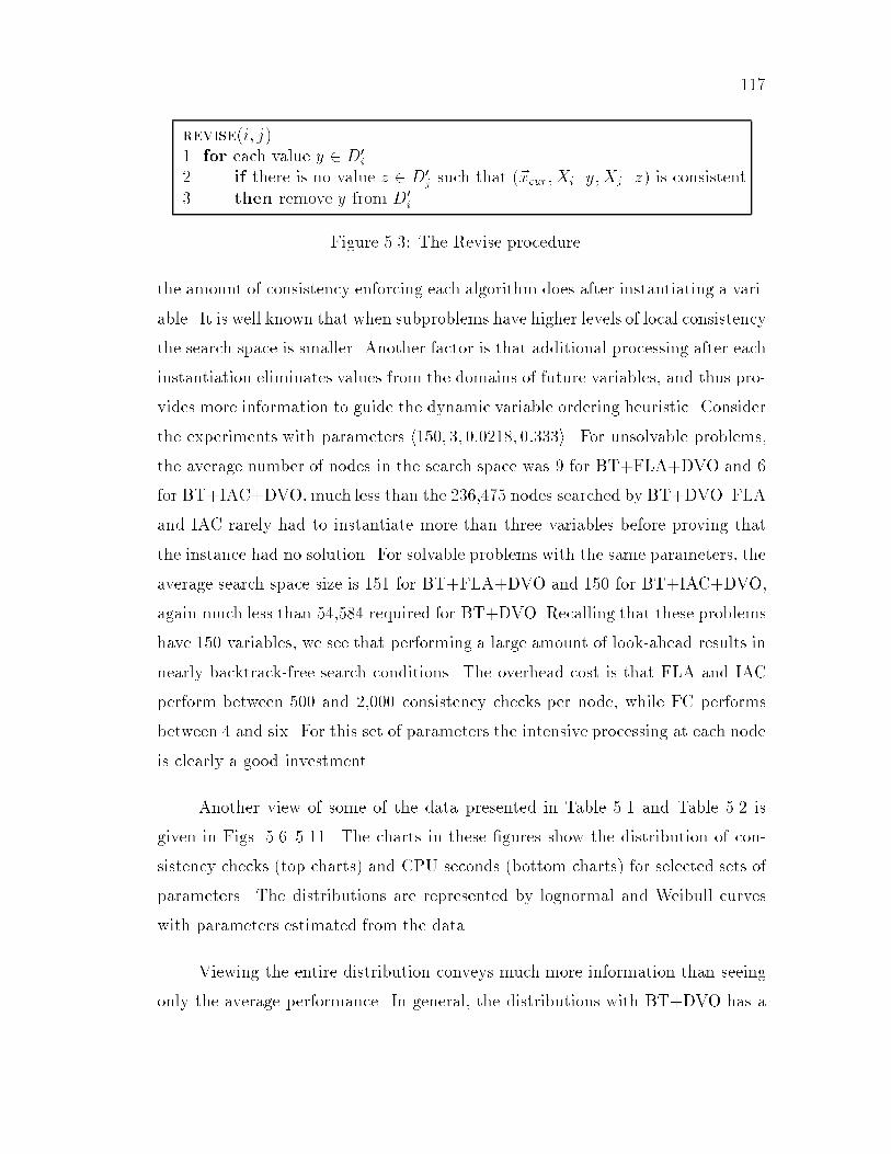
117

revise(i; j)1 for each value y 2 D0

i

2 if there is no value z 2 D0j such that (~xcur;Xi=y;Xj=z) is consistent

3 then remove y from D0i

Figure 5.3: The Revise procedure.

the amount of consistency enforcing each algorithm does after instantiating a vari-

able. It is well known that when subproblems have higher levels of local consistency

the search space is smaller. Another factor is that additional processing after each

instantiation eliminates values from the domains of future variables, and thus pro-

vides more information to guide the dynamic variable ordering heuristic. Consider

the experiments with parameters h150; 3; 0:0218; 0:333i. For unsolvable problems,

the average number of nodes in the search space was 9 for BT+FLA+DVO and 6

for BT+IAC+DVO,much less than the 236,475 nodes searched by BT+DVO. FLA

and IAC rarely had to instantiate more than three variables before proving that

the instance had no solution. For solvable problems with the same parameters, the

average search space size is 151 for BT+FLA+DVO and 150 for BT+IAC+DVO,

again much less than 54,584 required for BT+DVO. Recalling that these problems

have 150 variables, we see that performing a large amount of look-ahead results in

nearly backtrack-free search conditions. The overhead cost is that FLA and IAC

perform between 500 and 2,000 consistency checks per node, while FC performs

between 4 and six. For this set of parameters the intensive processing at each node

is clearly a good investment.

Another view of some of the data presented in Table 5.1 and Table 5.2 is

given in Figs. 5.6{5.11. The charts in these �gures show the distribution of con-

sistency checks (top charts) and CPU seconds (bottom charts) for selected sets of

parameters. The distributions are represented by lognormal and Weibull curves

with parameters estimated from the data.

Viewing the entire distribution conveys much more information than seeing

only the average performance. In general, the distributions with BT+DVO has a

118

full-looking-ahead(d)1 for i d + 1 to n2 for j d+ 1 to n3 revise(i; j)4 if D0

i = ;5 then return

Figure 5.4: The full looking ahead algorithm.

higher � for unsolvable problems and a lower � for solvable problems than do the

distributions with greater consistency enforcing. High values of � and low values

of � re ect greater skewness in the data. We see in these experiments that the

impact of additional look-ahead is most pronounced on the hardest problems in

the distribution's tail.

In Fig. 5.7, the y-axis indicates the proportional frequency of problems mak-

ing the number of consistency check or requiring the CPU time indicated on the

x-axis. The curve labeled \BT+DVO" on the top chart of this Figure shows that

with this algorithm a large proportion of the problems used less than 62,500 consis-

tency checks. Of the four algorithms, the curves show that more problems required

a small number of consistency checks with BT+DVO than with the other algo-

rithms. Nevertheless, the mean number of consistency checks, for these problems,

was higher with BT+DVO than with FLA or IAC (see Table 5.1). The reason

is that the BT+DVO lognormal curve has a \heavier" tail than that of the other

two algorithms. In other words, the hardest problems for BT+DVO are harder

partial-looking-ahead(d)1 for i d + 1 to n2 for j i+ 1 to n3 revise(i; j)4 if D0

i = ;5 then return

Figure 5.5: The partial looking ahead algorithm.

119

than the hardest problem for FLA or IAC (measuring consistency checks), and

this brings up the average for BT+DVO.

On problems with high C and low T , the extra work of arc-consistency can be

detrimental, while the bene�ts are great when C is low and T is high [86]. Table 5.3

shows some relevant statistics gleaned from instrumenting the BT+DVO+IAC

procedure. The �rst statistic, \Ratio CC / VR," measures the average number of

consistency checks performed by AC-3 for each value removed from the domain of a

future variable. When this measure is high, arc-consistency is relatively ine�cient.

The ratio tends to be lower with higher values of T .

The primary reason for performing interleaved arc-consistency, or indeed

any amount of look-ahead, is to recognize future dead-ends. The second statis-

tic, \Probability Empty Domain," in Table 5.3 shows how frequently the arc-

consistency procedure uncovers a future dead-end that was not discovered �rst by

forward checking style look-ahead. The table shows that this probability increases

with smaller C and higher T . We also note that it tends to be lower for D=6 than

for D=3, which is not surprising, since variables with larger domains are less likely

to have all values removed, other factors being equal.

120

h175; 3; 0:0358; 0:222iBT+DVO: �=2:57e-5 �=0:31 �=971BT+PLA+DVO: �=2:91e-6 �=0:40 �=76,754BT+FLA+DVO: �=4:08e-6 �=0:81 �=102,459BT+IAC+DVO: �=5:41e-6 �=0:83 �=106,748

0 62,500 250,000 437,500Consistency Checks

Frequency

.1

.2

.3

BT+DVO

PLA

FLA

IAC

h175; 3; 0:0358; 0:222iBT+DVO: �=0:79 �=0:27 �=0BT+PLA+DVO: �=1:23 �=0:30 �=0.43BT+FLA+DVO: �=1:07 �=0:75 �=0.65BT+IAC+DVO: �=5:44 �=0:73 �=0.20

0 1.25 5 8.75CPU Seconds

Frequency

.1

.2

.3

BT+DVO

IAC

PLA

FLA

Figure 5.6: Weibull curves based on solvable problems generated from parametersh175; 3; 0:0358; 0:222i. The top chart is based on consistency checks, the bottomchart on CPU seconds. �, �, and � parameters were estimated using the Modi�edMoment Estimator (see Chapter 3).

121

h175; 3; 0:0358; 0:222iBT+DVO: �=11:19 �=1:45BT+PLA+DVO: �=13:64 �=1:07BT+FLA+DVO: �=12:64 �=0:86BT+IAC+DVO: �=12:30 �=0:98

0 62,500 250,000 437,500Consistency Checks

Frequency

.01

.02BT+DVO

PLA

FLA

IAC

h175; 3; 0:0358; 0:222iBT+DVO: �=0:48 �=1:68BT+PLA+DVO: �=1:41 �=1:12BT+FLA+DVO: �=0:30 �=0:89BT+IAC+DVO: �=�1:32 �=0:96

0 1.25 5 8.75CPU seconds

Frequency

.01

.02

BT+DVO

PLA

FLA

IAC

Figure 5.7: Lognormal curves based on unsolvable problems generated from pa-rameters h175; 3; 0:0358; 0:222i. The top chart is based on consistency checks, thebottom chart on CPU seconds. � and � parameters were estimated using theMaximum Likelihood Estimator (see Chapter 3).

122

h60; 6; 0:2192; 0:222iBT+DVO: �=1:10e-6 �=1:04 �=1,202BT+PLA+DVO: �=1:38e-7 �=1:04 �=11,026BT+FLA+DVO: �=1:50e-7 �=1:05 �=18,236BT+IAC+DVO: �=1:49e-7 �=1:07 �=20,348

0 1,250,000 5,000,000 8,750,000Consistency Checks

Frequency

.01

.02

.03

.04

BT+DVO

PLA, FLA, and IAC

h60; 6; 0:2192; 0:222iBT+DVO: �=0:29 �=1:02 �=0.0BT+PLA+DVO: �=0:11 �=1:04 �=0.0BT+FLA+DVO: �=0:13 �=1:05 �=0.0BT+IAC+DVO: �=0:15 �=1:06 �=0.0

0 2.5 10 17.5CPU seconds

Frequency

.01

.02BT+DVO

PLAFLA

IAC

Figure 5.8: Weibull curves based on solvable problems generated from parametersh60; 6; 0:2192; 0:222i. The top chart is based on consistency checks, the bottomchart on CPU seconds. �, �, and � parameters were estimated using the Modi�edMoment Estimator (see Chapter 3). The PLA, FLA, and IAC curves on the topchart are almost indistinguishable.

123

h60; 6; 0:2192; 0:222iBT+DVO: �=14:30 �=0:47BT+PLA+DVO: �=16:38 �=0:46BT+FLA+DVO: �=16:30 �=0:44BT+IAC+DVO: �=16:32 �=0:43

0 2,500,000 10,000,000 17,500,000Consistency Checks

Frequency

.01

.02

.03

.04

.05

BT+DVO

PLA, FLA, IAC

h60; 6; 0:2192; 0:222iBT+DVO: �=1:81 �=0:49BT+PLA+DVO: �=2:78 �=0:46BT+FLA+DVO: �=2:61 �=0:44BT+IAC+DVO: �=2:50 �=0:44

0 2.5 10 17.5CPU seconds

Frequency

.005

.01BT+DVO

PLAFLAIAC

Figure 5.9: Lognormal curves based on unsolvable problems generated from pa-rameters h60; 6; 0:2192; 0:222i. The top chart is based on consistency checks, thebottom chart on CPU seconds. � and � parameters were estimated using theMaximum Likelihood Estimator (see Chapter 3). The PLA, FLA, and IAC curveson the top chart are almost indistinguishable.

124

h75; 6; 0:1038; 0:333iBT+DVO: �=2:04e-6 �=0:80 �=1,573BT+PLA+DVO: �=3:63e-7 �=0:83 �=35,719BT+FLA+DVO: �=5:65e-7 �=0:83 �=55,344BT+IAC+DVO: �=5:83e-7 �=0:84 �=57,869

0 500,000 2,000,000 3,500,000Consistency Checks

Frequency

.01

.02

.03

.04

.05

.06

.07

FLA and IAC

BT+DVO

PLA

h75; 6; 0:1038; 0:333iBT+DVO: �=0:29 �=0:80 �=0.01BT+PLA+DVO: �=0:20 �=0:83 �=0.07BT+FLA+DVO: �=0:35 �=0:84 �=0.10BT+IAC+DVO: �=0:64 �=0:83 �=0.06

0 1 4 7Seconds

Frequency

.01

.02

.03

.04

BT+DVOFLA

PLA

IAC

Figure 5.10: Weibull curves based on solvable problems generated from parametersh75; 6; 0:1038; 0:333i. The top chart is based on consistency checks, the bottomchart on CPU seconds. �, �, and � parameters were estimated using the Modi�edMoment Estimator (see Chapter 3). The FLA and IAC curves on the top chartare almost indistinguishable.

125

h75; 6; 0:1038; 0:333iBT+DVO: �=13:32 �=0:79BT+PLA+DVO: �=15:10 �=0:72BT+FLA+DVO: �=14:72 �=0:68BT+IAC+DVO: �=14:71 �=0:67

0 1,000,000 4,000,000 7,000,000Consistency Checks

Frequency

.01

.02

.03

.04

PLA

FLA and IAC

BT+DVO

h75; 6; 0:1038; 0:333iBT+DVO: �=1:39 �=0:78BT+PLA+DVO: �=1:86 �=0:72BT+FLA+DVO: �=1:38 �=0:68BT+IAC+DVO: �=0:78 �=0:69

0 2.5 10 17.5CPU seconds

Frequency

.01

.02

.03

BT+DVO

PLA

FLA

IAC

Figure 5.11: Lognormal curves based on unsolvable problems generated from pa-rameters h75; 6; 0:1038; 0:333i. The top chart is based on consistency checks, thebottom chart on CPU seconds. � and � parameters were estimated using theMaximum Likelihood Estimator (see Chapter 3). The FLA and IAC curves on thetop chart are almost indistinguishable.

126

The statistics in Table 5.3 show that when C is high and T is low, interleav-

ing arc-consistency does many extra consistency checks for very little pay-o�, as

measured by dead-ends discovered. With low C and high T the AC-3 procedure

is more e�cient and produces a greater bene�t.

Ratio ProbabilityParameters CC / VR Empty Domainh125; 3; 0:1199; 0:111i 81.2 0.0000h175; 3; 0:0358; 0:222i 33.4 0.0715h150; 3; 0:0218; 0:333i 19.1 0.1844h40; 6; 0:7308; 0:111i 191.8 0.0000h60; 6; 0:2192; 0:222i 100.4 0.0012h75; 6; 0:1038; 0:333i 59.7 0.0420h100; 6; 0:0497; 0:444i 40.0 0.0956h100; 6; 0:0391; 0:556i 31.8 0.1771

Table 5.3: Statistics from experiments in Figs. 5.1 and 5.2; just algorithmBT+DVO+IAC; solvable and unsolvable instances combined. The \Ratio CC /VR" column shows the ratio of consistency checks (CC) during the arc-consistencyprocedure to domain values removed (VR) during arc-consistency. \ProbabilityEmpty Domain" reports the observed probability that performing arc-consistencycreated an empty domain in a future variable.

Table 5.1 and Table 5.2 show only one large value ofN for each combination of

D and T . To show that these numbers are indicative of the trend with increasingN .

Fig. 5.12 presents the results of experiments with BT+DVO, BT+DVO+FLA, and

BT+DVO+IAC over a variety of values of N . The �gure shows consistency checks

and nodes expanded in the search tree, as well as CPU time. An approximately

linear relationship between N and the logarithm of each measure is apparent, with

the exception of BT+DVO on problems with T=:333. In this case the slope of

the trend line increases around N=100, although more data points are required to

determine whether or not the trend continues.

127

5.5 Variants of Interleaved Arc-consistency

The experiments presented so far in the chapter have demonstrated that the

relative e�ectiveness of di�erent consistency enforcing techniques is sensitive to

the number of constraints in a CSP and the tightness of those constraints. In this

section we de�ne and evaluate several heuristics designed to adapt the amount

of look-ahead in a dynamic fashion to the characteristics of the current prob-

lem. Our approach is to modify BT+IAC+DVO so that the amount of constraint

propagation can vary between forward checking and full arc-consistency. Before

turning to these heuristics, we �rst introduce a modi�cation to the Interleaved

Arc-consistency algorithm that improves its performance.

5.5.1 Domain checking

Our �rst modi�cation to BT+IAC+DVO is quite simple, and is based on the

observation that the AC-3 algorithm is most e�cient when the queue of unexam-

ined variable, called Q, is as small as feasible. As presented in Fig. 5.2, every future

variable is entered in Q after a new variable is instantiated. A better idea is to

put into Q, after each instantiation, only those variables which had a domain value

removed during step 2 (c) of BT+DVO. This change is re ected in Fig. 5.13 and

Fig. 5.14, which show a modi�ed version of step 2 (c) and of the AC-3 procedure.

We call the new arc-consistency procedure AC-DC, for domain checking.

Because the variables omitted from the queue Q by AC-DC are those which

did not have any values removed by the forward checking style look-ahead, and

which thus have no impact on the arc-consistency processing, BT+IAC+DVOwith

AC-DC explores exactly the same search space as BT+IAC+DVOwith AC-3. The

di�erence is in the number of consistency checks which need to be made, and in

the CPU time required to solve a CSP instance. In general, using AC-DC requires

about half as much CPU time as using AC-3. We present in Table 5.4, the results

128

T =

:111

CC

25 50 75 100 125

104

105

106

���� �

�����

�����

NODES

25 50 75 100 125

100

103

104

�����

�����

�����

CPU

25 50 75 100 125

:01

:1

1

10

�����

�����

�����

T=

:222

CC

25 50 100 150

103

104

105

�� �

�

� �

��� �

� �

�� �

�� �

NODES

25 50 100 150

100

103

104

�� �

�

� �

� �� �

� �

� �� �

� �

CPU

25 50 100 150

:01

:1

1

10

� ��

�

� �

�� �

�� �

�� �

�� �

T =

:333

CC

25 50 75 100 150

103

104

105

� ���

� �

�� �

� � �

�� �

� � �

NODES

25 50 75 100 150

100

103

104

105

� ���

� �

� � �� � �

� � �� � �

CPU

25 50 75 100 150

:01

:1

1

10

� ���

� �

� �� �

� �

� �� � � �

Figure 5.12: Comparison of BT+DVO (�), BT+DVO+FLA (�), andBT+DVO+IAC (�). Each data point is the mean of 500 solvable and unsolv-able instances generated with D=3, T=:111 (�rst row), T=:222 (second row) orT=:333 (third row), and N as indicated along the x-axis. Parameter C was setto the cross-over point. The left boxes on each row show consistency checks, themiddle boxes show nodes expanded in the search tree, and the right boxes showCPU time in seconds. Note that the y-axes are logarithmic.

129

Backtracking with DVO and varying amount of arc-consistency

2. Select a value . . .

(c) (Forward checking style look-ahead) Examine the future variablesXi; cur < i � n, For each v in D0

i, if Xi = v con icts with ~xcur thenremove v from D0

i and add Xi to Q; if D0i is now empty, go to (e)

(without examining other Xi's).

(d) (Additional looking ahead.)

iv. Else if Algorithm = IAC-DC perform ac-dc(i);

v. Else if Algorithm = IAC-UNIT perform ac-unit(i);

vi. Else if Algorithm = IAC-TRUNCATE performac-truncate(i);

vii. Else if Algorithm = IAC-FLA perform ac-fla(i).

Figure 5.13: Extended version of Fig. 5.1.

of an empirical comparison of the two variations of interleaving arc-consistency, as

well as plain BT+DVO and several other variations described below. Because we

did not �nd any signi�cant di�erence in the performance of these algorithms on

solvable and unsolvable problems, we combine both types in Table 5.4. Note that

the generator parameters used in the Table 5.4 experiments are similar to those in

Figs. 5.1 and 5.2, but have larger values of N .

ac-dc(d)1 repeat2 select and delete any arc(p; q) in Q3 revise(p; q)4 if D0

p = ;5 then return6 if revise removed a value from D0

p

7 then Q Q [ farc(i; p)ji > dg8 until Q = ;

Figure 5.14: Algorithm AC-DC, a modi�cation of AC-3.

130

5.5.2 The unit variable heuristic

The intuition behind the unit variable heuristic (IAC-U) is closely coupled

to the dynamic variable ordering scheme. One advantage of performing more

look-ahead is that more values in the domains of future variables are removed.

Consequently, the dynamic variable ordering heuristic is more likely to be e�ective.

In the absence of a dead-end, we hope to �nd a future variable with a domain size

of 1, as instantiating this single value represents a forced choice that will have to be

made eventually. The unit variable heuristic terminates its consistency enforcing

when the current domain of some future variable becomes 0 or 1. A future variable

with only one value is called a \unit" variable. If a dead-end or unit variable is

found, that variable will become the next in the ordering. The goal is to do enough

looking ahead to guide e�ectively the variable ordering heuristic.

ac-unit(d)0.1 if any future variable has domain size 10.2 then return1 repeat2 select and delete any arc(p; q) in Q3 revise(p; q)4 if D0

p = ; or jD0pj = 1

5 then return6 if revise removed a value from D0

p

7 then Q Q [ farc(i; p)ji > dg8 until Q = ;

Figure 5.15: Algorithm AC-DC with the unit variable heuristic.

Only two changes are required to the AC-DC algorithm in Fig. 5.14 to im-

plement the unit variable heuristic (see Fig. 5.15). Lines 0.1 and 0.2 check for any

future variable with only one value it its domain, and if one is found the algorithm

returns. Line 4 is modi�ed to test if the variable on which arc-consistency has just

been enforced has just one value left; again the procedure returns immediately if

so.

131

Empirical results of using the unit variable heuristic are reported in Table 5.4.

CPU time for IAC with the heuristic was between BT+DVO and BT+IAC+DVO

in seven out of eight parameter settings. Similar results hold on an instance by

instance basis. Over all eight sets of parameters, including h75; 6; :1744; :222i,where using the unit variable heuristic produced average CPU time worse than

both BT+DVO and BT+IAC+DVO, 87% of individual instance CPU times with

the heuristic were between the CPU times of BT+DVO and BT+IAC+DVO.

Unfortunately, using the unit variable heuristic severely degraded the perfor-

mance of BT+IAC+DVO on problems with relatively tight constraints. Stopping

the arc-consistency procedure after a unit variable is produced is often harmful,

largely because further processing often uncovers a variable with an empty domain,

and the resulting dead-end cuts o� an unfruitful branch of the search tree.

5.5.3 The full looking ahead method

Another method for guiding IAC to a reduced amount of arc-consistency can

be developed by combining full looking ahead with AC-3's Q data structure. The

result, called IAC-FLA, is a variant of IAC which performs a single pass over the

Q set (see Fig. 5.16). Just as full looking ahead does not consider the impact of

future variables on other future variables, IAC-FLA does not add variables to Q

when they are modi�ed by revise.

ac-fla(d)1 repeat2 select and delete any arc(p; q) in Q3 revise(p; q)4 if D0

p = ;5 then return6 until Q = ;

Figure 5.16: Algorithm AC-DC, with the full looking ahead method.

132

T=1/9T=2/9

T=3/9

10 25 50 75 100 125 150

:1

:2

Figure 5.17: The fraction of future variable domain values removed by IAC (alongthe y-axis), as a function of depth in the search tree (along the x-axis). Each linerepresents the mean over 500 instances, for a single set of parameters with T=3,D=1/9, 2/9 or 3/9, and N and C as in Table 5.1.

The goal of achieving performance between BT+DVO and BT+IAC+DVO

was largely achieved with IAC-FLA. Nevertheless, the results of IAC-FLA are

unsatisfactory { slightly worse than IAC-U in all but one case in Table 5.4. As with

IAC-U, it seems that this heuristic is often causing useful constraint propagation

to be bypassed.

5.5.4 The truncation heuristic

To help us understand why IAC is better for certain classes of problem than

for others, we modi�ed our program to report what fraction of the values in the

domains of future variables are removed during arc-consistency process. This frac-

tion is a measure of the e�ectiveness of arc-consistency. In terms of the revise

procedure in Fig. 5.3, we measured the ratio of times a value y is removed in line 3

to the number of values y considered in line 1. We tabulated this ratio relative to

the value of d, the depth in the search tree which is a parameter to AC-DC. The

results are shown in Fig. 5.17.

Studying Fig. 5.17 prompted the observation that when arc-consistency is

most successful, that is, for T=3/9, most of its power seems to come at shallow

133

levels in the search tree, where d is small. When the constraints are loose, e.g.

T=1/9, arc-consistency is most likely to remove values somewhat deeper in the

tree, but in such cases the cost to do so does not seem to be justi�ed. Thus it

seems that the most useful time to perform arc-consistency is after instantiating

variables relatively high in the search tree. Interestingly, this conclusion seems to

be counter to the intuition of Gaschnig, who proposed doing backtracking on the

top of the tree and adding arc-consistency lower in the tree [31].

ac-truncate(d)1 if d � 102 then return3 perform AC-DC

Figure 5.18: Algorithm AC-DC with the truncation heuristic.

We therefore developed a heuristic for IAC called truncation. The modi�-

cation is simple: arc-consistency is performed only when the newly instantiated

variable is at depth 10 or less in the search tree (see Fig. 5.18). At depth greater

than 10, BT+IAC+DVO with truncation is identical to BT+DVO.

The truncation heuristic did not turn out to be a good performer in our

experiments (see Table 5.4). We also tried truncation levels other than 10, but

with no improvement. We were unable to complete the experiments with the

truncation heuristic for some sets of parameters, because dozens of instances were

taking several hours each.

5.5.5 Experimental comparison

We compared the algorithms and heuristics described above using a variety

of parameters for the random problem generator. The average results are reported

in Table 5.4. This table does not separate results for satis�able and unsatis�able

instances, since we observed the same overall behavior on both types of problems.

134

Parameters BT+DVO IAC IAC-DC IAC-U IAC-F IAC-Th150; 3; :0995; :111i 3.02 19.55 8.99 7.07 10.50 7.38h200; 3; :0313; :222i 3.77 1.92 4.05 8.60 12.78h200; 3; :0160; :333i 3.53 1.01 12.29 19.83h50; 6; :5794; :111i 3.89 20.69 12.74 4.93 7.08 8.19h75; 6; :1744; :222i 17.50 41.28 15.92 23.44 29.00 25.01h90; 6; :0861; :333i 51.66 8.83 3.99 7.25 8.99 43.17h125; 6; :0395; :444i 4.04 2.51 8.87 10.55h150; 6; :0209; :556i 6.38 4.34 29.45 26.15

Table 5.4: Comparison, by mean CPU seconds, of six algorithms basedon BT+DVO: regular BT+DVO, BT+DVO with interleaved arc-consistencyusing AC-3 (IAC), BT+DVO with interleaved arc-consistency using domainchecking (IAC-DC), BT+IAC+DVO-DC with the unit variable heuristic (IAC-U), BT+IAC+DVO-DC with the full looking ahead heuristic (IAC-F), andBT+IAC+DVO-DC with truncation at level 10 (IAC-T). Each number is the meanof 500 satis�able and unsatis�able instances. The best time in each row is in bold-face. The BT+DVO and IAC-T positions are blank when we were unable to runall instances because too much CPU time was required.

On the problems in these experiments, the best combination was BT+DVO+IAC-

DC, which had the lowest mean CPU time in six out of eight sets of problems.

5.6 Conclusions

In this chapter we studied one of the most intriguing questions in solving

CSPs: what is the right balance between search and consistency enforcing? How

can we make consistency enforcing cost-e�ective most of the time? We cannot

provide de�nitive answers to these questions, but our experiments provide some in-

sight into how they will be resolved for any particular problem or class of problems.

We examined several known consistency methods interleaved with BT+DVO. We

showed that when the constraints were tight and relatively few, interleaving an

arc-consistency procedure after each instantiation was very e�ective on the prob-

lems we tested. In particular, a new variation of AC-3 called AC-DC reduced the

number of consistency checks and was especially e�ective. When the constraints

135

were loose and there were many constraints, arc-consistency was detrimental, and

the best choice was to use lower levels of consistency, such as forward checking in

the BT+DVO algorithm. Because the experiments were all conducted at the 50%

satis�able cross-over point, they cannot be considered a reliable guide to other

regions of the parameter space.

We also studied several consistency enforcing approaches that lie between

forward checking and interleaving arc-consistency in the amount of work performed

after each instantiation. Ideally an intermediate approach would always perform

close to the better of BT+DVO and BT+IAC+DVO. Two such algorithms were

proposed by Haralick and Elliott: full looking ahead and partial looking ahead. We

proposed three new heuristics: the unit variable heuristic, the full looking ahead

heuristic, and the truncation heuristic. On the problems we used none of these

techniques were successful enough to dislodge BT+DVO and BT+IAC+DVO as

the algorithms of choice when looking ahead.

An important question is whether the addition of backjumping would improve

the performance of an interleaved arc-consistency algorithm. On the problems

we have experimented with the answer is probably no, because IAC reduces the

search space so much that few opportunities arise for large jumps; however, a

BJ+DVO+IAC algorithm might be e�ective on much larger problems.

Chapter 6

Look-ahead Value Ordering

6.1 Overview of the Chapter

Algorithms such as forward checking and integrated arc-consistency speed up

backtracking by causing dead-ends to occur earlier in the search, and by providing

information that is useful for dynamic variable ordering. In this chapter, we show

that another use of looking ahead is a domain value ordering heuristic, which

we call look-ahead value ordering or LVO1. LVO ranks the values of the current

variable, based on the number of con icts each value has with values in the domains

of future variables. Our experiments show that look-ahead value ordering can be

of substantial bene�t, especially on hard constraint satisfaction problems.

6.2 Introduction

In this chapter we present a new heuristic for prioritizing the selection of

values when searching for the solution of a constraint satisfaction problem. If a

constraint satisfaction problem has a solution, knowing the right value for each

variable would enable a solution to be found in a backtrack-free manner. When

a CSP has only a small number of solutions, much time is often spent search-

ing branches of the search space which do not lead to a solution. To minimize

1This work was �rst reported in Frost and Dechter [28].

136

137

backtracking, we should �rst try the values which are more likely to lead to a con-

sistent solution. Our new algorithm, look-ahead value ordering (LVO), implements

a heuristic that ranks the values of the current variable based on information gath-

ered during a forward checking style look-ahead, determining the compatibility of

each value with the values of all future variables. Although the heuristic does not

always correctly predict which values will lead to solutions, it is frequently more

accurate than an uninformed ordering of values. Our experiments show that while

the overhead of LVO usually outweighs its bene�ts on easy problems, the improve-

ment it provides on very large problems can be substantial. Interestingly, LVO

often improves the performance of backjumping on problems without solutions.

Look-ahead value ordering does the same type of look-ahead as does the

forward checking algorithm [40]. Because forward checking rejects values that it

determines will not lead to a solution, it can be viewed as doing a simple form

of value ordering. In this regard LVO is more re�ned, because it also orders the

values that may be part of a solution.

6.3 Look-ahead Value Ordering

Look-ahead value ordering ranks the values of the current variable, based

on the impact each value would have on the domains of the future variables.

Combining BJ+DVO with LVO results in BJ+DVO+LVO; a description of this

algorithm appears in Fig. 6.1. The algorithm is essentially the same as BJ+DVO

from Chapter 4; the di�erences are in steps 1A, 2 (b), and 2 (c).

Step 1A of BJ+DVO+LVO is where the algorithm's look-ahead phase takes

place. The current variable is tentatively instantiated with each value x in its

domain D0cur . BJ+DVO+LVO looks ahead, in a forward checking style manner,

to determine the impact each x will have on the D0 domains of uninstantiated

138

Backjumping with DVO and LVO0. (Initialize.) Set D0

i Di for 1 � i � n.

1. (Step forward.) If Xcur is the last variable, then all variables have valueassignments; exit with this solution. Otherwise, set cur to be the indexof the next variable, according to a variable-ordering-heuristic.Set Pcur ;.

1A. (Look-ahead value ordering.) Rank the values in D0cur as follows: For

each value x in D0cur, and for each value v of a future variables

Xi; cur < i � n, determine the consistency of (~xcur�1;Xcur=x;Xi=v).Using a heuristic function, compute the rank of x based on the numberand distribution of con icts with future values v.

2. Select a value x 2 D0cur. Do this as follows:

(a) If D0cur = ;, go to 3.

(b) Pop the highest ranked value x from D0cur and instantiate Xcur x.

(c) (This step can be avoided by caching the results from step 1A.)Examine the future variables Xi; cur < i � n. For each v in D0

i, ifXi = v con icts with ~xcur then remove v from D0

i and add Xcur toPi; if D0

i becomes empty, go to (d) without examining other Xi's.

(d) Go to 1.

3. (Backjump.) If Pcur = ; (there is no previous variable), exit with\inconsistent." Otherwise, set P Pcur; set cur equal to the index ofthe last variable in P . Set Pcur Pcur [ P �fXcurg. Reset all D0 sets tothe way they were before Xcur was last instantiated. Go to 2.

Figure 6.1: Backjumping with DVO and look-ahead value ordering (LVO).

variables. In section 6.4, we discuss three heuristic functions that can be called in

this step to rank the values.

In step 2 (b), the current variable is instantiated with the highest ranking

value. If the algorithm returns to a variable because of a backjump, the highest

ranked remaining value in its domain is selected. If the variable is re-instantiated

after earlier variables have changed, then the ranking of the values has to be

repeated in step 1A.

139

Step 2 (c) essentially disappears in BJ+DVO+LVO; once a value is actually

selected, it would not make sense to repeat the look-ahead that has already been

done. To avoid repeating consistency checks, our implementation saves in tables

the results of step 1A. After a value is chosen in 2 (b), the appropriate D0s and

P s of future variables are copied from these tables instead of being recomputed

in step 2(c). The space required for these tables is not prohibitive. BJ+DVO

uses O(n2d) space for the D0 sets, where d is the size of the largest domain: n

levels in the search tree (D0 is saved at each level so that it does not have to be

recomputed after backjumping) � n future variables � d values for each future

variable. Our implementation of BJ+DVO+LVO uses O(n2d2) space. There is an

additional factor of d because at each level in the search tree up to d values are

explored by look-ahead value ordering. Similarly, the space complexity for the P

sets increases from O(n2) in BJ+DVO to O(n2d) for BJ+DVO+LVO. To solve a

typical problem instance described in the next section, BJ+DVO required 1,800

kilobytes of random access memory, and BJ+DVO+LVO required 2,600 kilobytes.

On our computer the additional space requirements of LVO had no discernable

impact.

6.4 LVO Heuristics

We experimented with several LVO heuristics that rank values based on their

con icts with values of future variables.

The �rst heuristic, called min-con icts (MC), considers each value in D0cur

and associates with it the number of values in the D0 domains of future variables

with which it is not compatible. The current variable's values are then selected

in increasing order of this count. In other words, this heuristic chooses the value

which removes the smallest number of values from the domains of future variables.

140

The second heuristic is inspired by the intuition that a subproblem is more

likely to have a solution if it doesn't have variables with only one value. Each of

the search trees rooted at some instantiation of Xcur is a di�erent subproblem. A

variable with only one remaining value makes a subproblem \fragile," in the sense

that if that value is removed the subproblem has no solution. The max-domain-size

(MD) heuristic therefore prefers the value inD0cur that creates the largest minimum

domain size in the future variables. For example, if after instantiating Xcur with

value x1 the mini2fcur+1;...;ng jD0i j is 2, and with Xcur=x2 the min is 1, then x1 will

be preferred.

Our third heuristic function for selecting a value is based on the Advised

Backtracking (ABT) algorithm of Dechter and Pearl [18]. ABT uses an estimate

of the number of solutions in each subproblem to choose which value to instantiate

next. The ES (Estimate Solutions) heuristic for LVO computes an upper bound

on the number of solutions by multiplying together the domain size of each future

variable, after values incompatible with a value in D0cur have been removed. The

upper bound is higher than the actual number of solutions if there are constraints

between the future variables, as is usually the case. The value that leads to the

highest upper bound on the number of solutions is chosen �rst.

In addition to the three LVO heuristics, we also experimented with a static

value ordering heuristic we call static least-con icts (S-LC). We call this heuristic

static because it runs once, before search, and the order it assigns to the values

does not change. Values are ranked in ascending order by the number of values

of other variables with which they con ict. For instance, consider variable X1 in

the coloring problem of Chapter 2 (Fig. 2.2). Its value red con icts with three

values in other variables, blue con icts with four values, and green con icts with

one value. The S-LC heuristic will rank the values in order (green, red, blue), and

the values will always be considered in this order when X1 has to be instantiated.

We developed the S-LC heuristic as a \straw-man" so that we could compare LVO

heuristics against not just plain BJ+DVO, but also against BJ+DVO augmented

141

with a value ordering that was very cheap to compute. As described in the following

section, the S-LC heuristic performed quite well.

It is worth mentioning that we experimented with several other heuristics

which were not as good as those reported in this chapter. In general, we found

value ordering heuristics that seemed more \sophisticated" to be slightly poorer

in practice. For example, we tried modifying the MD heuristic with several tie-

breaking functions, because often more than one value results in the sameminimum

future domain size. Each tie breaker degraded the average performance of the

algorithm. We have no explanation for this puzzling result.

6.5 Experimental Results

6.5.1 Comparing LVO heuristics

We conducted an experiment to determine the relative performance of the

LVO heuristics. Eight sets of parameters near the cross-over point were selected,

and with each set we generated 500 random CSPs. Five algorithms were applied

to each instance: BJ+DVO (without a value ordering heuristic), BJ+DVO with

S-LC, and BJ+DVO+LVO with the three heuristics described in the previous

section. The results are reported in Tables 6.1 and 6.2. The tables show mean

CPU time; mean consistency checks and number of nodes correlated closely with

CPU time.

Tables 6.1 and 6.2 together contain 16 rows comparing the �ve algorithms.

BJ+DVO+LVO with the MC heuristic had the lowest CPU time in 9 out of 16

cases. Second best was BJ+DVO with the S-LC heuristic, which was best in 5 out

of 16. The MD and ES heuristics were each fastest in one case. The di�erences

in average CPU time were mostly relatively small, but MC was clearly the best

142

Mean CPU seconds (250 unsolvable instances)Parameters No VO S-LC LVO-MC LVO-MD LVO-ESh150; 3; :0995; :111i 11.90 11.40 12.50 12.28 13.39h200; 3; :0313; :222i 5.15 4.79 4.81 5.04 4.97h250; 3; :0125; :333i 14.88 8.52 8.03 12.00 8.44h50; 6; :5796; :111i 21.72 21.24 21.58 21.00 21.61h60; 6; :2192; :222i 10.53 10.48 10.37 10.38 10.62h75; 6; :1038; :333i 7.55 7.49 7.36 7.46 7.56h100; 6; :0497; :444i 13.48 12.07 11.49 12.70 11.91h100; 6; :0319; :556i 7.94 5.03 5.37 6.98 5.68

Table 6.1: Comparison of BJ+DVO without LVO (\No VO"), with a static least-con icts value ordering (\S-LC"), and with LVO using three heuristics describedin the text.

heuristic for BJ+DVO+LVO. In the rest of the chapter, reference to LVO implies

the MC heuristic.

6.5.2 Further experiments with LVO

We experimented further with value ordering by selecting several additional

sets of parameters and with each set generating 500 instances that were solved

with BJ+DVO, BJ+DVO+SLC, and BJ+DVO+LVO. Based on the experiments

in Tables 6.1 and 6.2, as well as other tests, we concluded that LVO is most e�ective

on problems with large numbers of variables, large domains, and near the cross-

over point. Problems with these characteristics tend to take a large amount of

computer time to solve. We adopted two strategies that allowed us to demonstrate

the value of LVO on problems that were not too computationally expensive. The

�rst strategy was to use problems with tight constraints and sparse constraint

graphs. For instance, problems at N=100 and D=12 at the cross-over point might

be extremely time consuming to solve, except that we used a small number (120,

or C=:0242) of extremely tight constraints (T=:764 or 110/144). Another method

for generating easier problems with large N and D is to select parameters that are

143

Mean CPU seconds (250 solvable instances)Parameters No VO S-LC LVO-MC LVO-MD LVO-ESh150; 3; :0995; :111i 5.46 4.09 4.53 5.58 4.76h200; 3; :0313; :222i 4.27 3.96 3.62 3.89 3.64h250; 3; :0125; :333i 1.85 1.00 0.86 1.40 0.79h50; 6; :5796; :111i 8.93 6.57 6.71 7.75 6.66h60; 6; :2192; :222i 5.28 4.01 3.83 4.94 4.04h75; 6; :1038; :333i 5.51 4.65 4.36 5.02 4.38h100; 6; :0497; :444i 9.81 8.60 8.22 10.09 8.01h100; 6; :0319; :556i 3.36 2.32 1.90 3.40 2.38

Table 6.2: Comparison of BJ+DVO without LVO (\No VO"), with a static least-con icts value ordering (\S-LC"), and with LVO using three heuristics describedin the text.

not exactly at the cross-over point. We used this approach for the experiment with

h100; 9; :0606; :444i, where C is 95% of the estimated cross-over value of :0672.

The results of these experiments are summarized in Table 6.3 (unsolvable

instances) and Table 6.4 (solvable instances). Because we used some parameter

combinations that were not at the cross-over point, two experiments with few or

no unsolvable problems do not appear in Table 6.3. Tables 6.3 and 6.4 are designed

to present a multi-faceted view of our experimental results, and therefore several

di�erent statistics are reported. The �rst column shows the four parameters to

the random problem generator in the format hN;D;C; T i, and the percentage of

instances that had solutions. The columns titled \Mean CC" and \Mean CPU"

show the average values for the count of consistency checks made and the number of

CPU seconds used (on a SparcStation 4, 110 MHz processor). Two columns show

the estimated values of the � and � parameters of the lognormal distribution, in

Table 6.3), and in Table 6.4 the estimated values of the � and � parameters of

the Weibull distribution (the � value has been multiplied by 1,000,000 to make

the units more convenient). These parameters are based on the distribution of

the number of consistency checks. As discussed in Chapter 3, in the lognormal

distribution the mean and the variance both increase with larger � and �. The

variance is particularly sensitive to increases in �. With the Weibull distribution,

144

Parameters Mean Parameters %% Solvable Algorithm CC CPU � � Besth150; 6; 0:0209; 0:556i No VO 2,476,071 76.13 12.27 2.55 34.349% S-LC 1,718,777 52.87 11.81 2.47 24.4

LVO 1,358,316 44.48 11.66 2.38 41.3h250; 3; 0:0236; 0:222i No VO 2,024,230 104.27 13.07 1.82 10.487% S-LC 1,630,480 83.12 12.88 1.78 85.1

LVO 1,484,038 92.47 12.79 1.80 4.5h100; 12; 0:0242; 0:764i No VO 592,041 12.42 10.80 2.10 41.464% S-LC 532,075 10.63 10.59 2.04 15.5

LVO 434,904 9.88 10.56 1.96 43.1

Table 6.3: Results of several experiments on CSPs with various parameters; thistable show results for unsolvable problems.

a larger value of � or � results in smaller mean and variance. The �nal column in

the tables indicates the relative frequency with which each algorithm had the best

CPU time.

The experiments indicate that using either value order technique substan-

tially improves the performance of BJ+DVO on these relatively large problems,

both on problems with solutions and on those which do not have solutions. In all

but one case, unsolvable problems with parameters h250; 3; :0236; :222i, the rankingby either consistency checks or CPU time is BJ+DVO+LVO �rst, BJ+DVO+S-LC

second, and plain BJ+DVO last. The data in the \% Best" column indicate that

even when the presence of LVO substantially improves the mean performance of

BJ+DVO, on an instance by instance basis LVO does not always help; in fact, in

only one case, h100; 9; :0638; :444i, does LVO beat the other two algorithms in more

than half the instances. Moreover, according to the estimated � and � parameters,

adding LVO (or S-LC) to BJ+DVO does not result in a substantial impact on the

overall shape of the distribution of computational e�ort.

To understand how LVO a�ects the entire set of random CSP instances and

produces substantially lower means in consistency checks and CPU time, it is

important to take into account the extremely skewed nature of the distributions.

145

Consistency Checks

BJ+DVO� � BJ+DVO+LVO� �% of times LVO is worse

1 2 3 4 5 6 7 8 9 10

104

105

106

107

LVO worse100%

75%

50%

25%

0%

h100; 12; :0242; :764i

� � � � � � ���

�

��� �

� � � ��

�

Figure 6.2: The 500 instances in one experiment were divided into 10 groups, basedon the number of consistency checks made by BJ+DVO. Each point is the meanof 50 instances in one group; its position is based on the left-hand scale, whichis logarithmic. The dotted line, showing the percentage of times BJ+DVO wasbetter than BJ+DVO+LVO when measuring consistency checks, is related to theright-hand scale.

Consistency Checks

- BJ+DVO+LVO

Consistency Checks - BJ+DVO104 105 106 107 108

104

105

106

107

108h100; 12; :0242; :764i

�

��

�

�

� ��

�

�

��

�

��

�

���

�

��

�

����

� ��

�

��������

��

��

��

�

� ��

�

����

�

��

�

�

��

�

� ��

�

���

�

�����

��

�

�

����

�

�

��

�

�� ��

���

����

�

�

�

���

��

�

�

�

�

��

��

�

� ���

�

�����

�

�

��� ���

��

�

�

�

����

�

�

�

�

�

���

�

�

�

����

���

����

��

�

� �

��

�

�

���

����

�

��

�

�

�

�

�

�

�

�

��

�

�

�

�

�

�

�

�

��

�

�

�

�

�

�

��

�

�

�

�

�

�

��

�

�

��

�

�

�

�

�

�

�

��

�

��

�

�

� ��

�

�

�

�

�

�

�

�

�

�

�

�

�

�

�

�

�

�

�

�

�

�

�

�

��

��

�

� �

��

��

�

� �

�

�

�

�

�

�

�

��

�

�

�

��

�

�

��

�

�

�

�

�

�

�

�

��

�

�

�

�

�

��

�

��

�

�

��

�

�

�

�

�

�

�

�

�

�

��

�

�

�

��

�

�

�

�

�

�

�

�

�

�

�

��

�

�

�

�

�

�

�

�

�

�

�

�

�

�

�

� ��

�

�

�

��

�

�

�

��

�

�

�

�

���

�

�

�

��

��

�

�

�

�

�

�

�

��

�

�

�

�

�

�

�

�

�

�

�

�

�

��

�

�

�

�

�

�

��

�

�

�

��

�

�

��

��

�

�

�

�

�

�

�

�

�

�

�

�

�

��

�

�

�

�

�

�

�

��

�

�

�

� �

� ���

�

�

�

�

� �

�

�

�

�

�

�

�

�

�

�

�

�

�

�

�

�

�

�

�

�

�

�

�

��

Figure 6.3: Each point (� = has solution, � = no solution) represents one instanceout of 500. Note that both axes use logarithmic scales. Points below the diagonalline required fewer consistency checks with LVO.

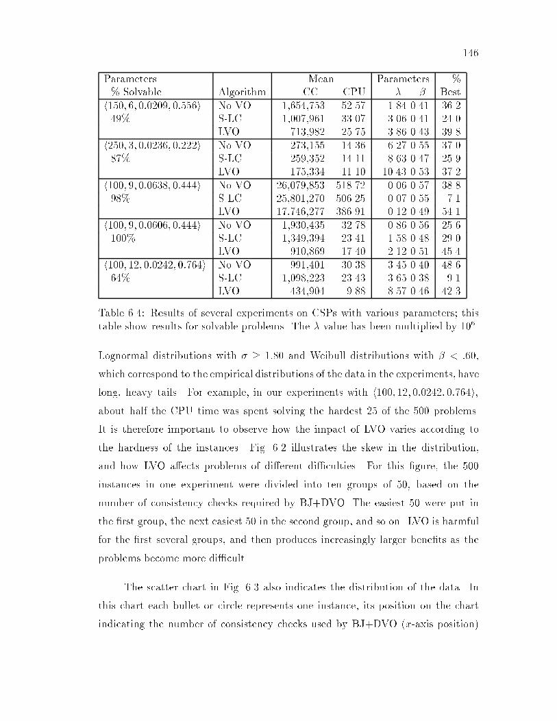
146

Parameters Mean Parameters %% Solvable Algorithm CC CPU � � Besth150; 6; 0:0209; 0:556i No VO 1,654,753 52.57 1.84 0.41 36.249% S-LC 1,007,961 33.07 3.06 0.41 24.0

LVO 713,982 25.75 3.86 0.43 39.8h250; 3; 0:0236; 0:222i No VO 273,155 14.36 6.27 0.55 37.087% S-LC 259,352 14.11 8.63 0.47 25.9

LVO 175,334 11.10 10.43 0.53 37.2h100; 9; 0:0638; 0:444i No VO 26,079,853 518.72 0.06 0.57 38.898% S-LC 25,801,270 506.25 0.07 0.55 7.1

LVO 17,746,277 386.91 0.12 0.49 54.1h100; 9; 0:0606; 0:444i No VO 1,930,435 32.78 0.86 0.56 25.6100% S-LC 1,349,394 23.41 1.58 0.48 29.0

LVO 910,869 17.40 2.12 0.51 45.4h100; 12; 0:0242; 0:764i No VO 991,401 30.38 3.45 0.40 48.664% S-LC 1,098,223 23.43 3.65 0.38 9.1

LVO 434,904 9.88 8.57 0.46 42.3

Table 6.4: Results of several experiments on CSPs with various parameters; thistable show results for solvable problems. The � value has been multiplied by 106.

Lognormal distributions with � � 1:80 and Weibull distributions with � < :60,

which correspond to the empirical distributions of the data in the experiments, have

long, heavy tails. For example, in our experiments with h100; 12; 0:0242; 0:764i,about half the CPU time was spent solving the hardest 25 of the 500 problems.

It is therefore important to observe how the impact of LVO varies according to

the hardness of the instances. Fig. 6.2 illustrates the skew in the distribution,

and how LVO a�ects problems of di�erent di�culties. For this �gure, the 500

instances in one experiment were divided into ten groups of 50, based on the

number of consistency checks required by BJ+DVO. The easiest 50 were put in

the �rst group, the next easiest 50 in the second group, and so on. LVO is harmful

for the �rst several groups, and then produces increasingly larger bene�ts as the

problems become more di�cult.

The scatter chart in Fig. 6.3 also indicates the distribution of the data. In

this chart each bullet or circle represents one instance, its position on the chart

indicating the number of consistency checks used by BJ+DVO (x-axis position)

147

Consistency

Checks

number of variables (N)

BJ+DVO� � BJ+DVO+LVO� �

50 75 100104

105

106

�

� �

�

���

�D=12T=.0490

100 200 300

103

104

105

106

�������

�������

D=3T=.333

Figure 6.4: The bene�ts of LVO increases on problems with more variables. Eachpoint is the mean of 500 instances. C is always set to the cross-over point. y-axisis logarithmic.

and by BJ+DVO+LVO (y-axis position). Many instances lie along or near the

diagonal, demonstrating an approximately equal performance by both algorithms.

Several dozen instances are very easy for one algorithm, requiring around 100 to 200

consistency checks, and somewhat harder for the other, requiring up to 100,000

consistency checks. The overall means are strongly a�ected by a few instances,

both solvable and unsolvable, which require 10 or more times as much work with

BJ+DVO than with BJ+DVO+LVO.

Figs. 6.2 and 6.3 show data drawn from just one set of parameters. The pat-

tern of data from experiments with other parameters is quite similar. The overall

conclusion we draw from our experiments with BJ+DVO and BJ+DVO+LVO is

that on su�ciently di�cult problems LVO almost always produces substantial im-

provement; on medium problems LVO usually helps but frequently hurts; and on

easy problems the overhead of LVO is almost always worse than the bene�t. Very

roughly, \su�ciently di�cult" is over 1,000,000 consistency checks and \easy" is

under 10,000 consistency checks.

In general the statistics for CPU time are slightly less favorable for LVO

than are the statistics for Consistency Checks, re ecting the fact that, in our

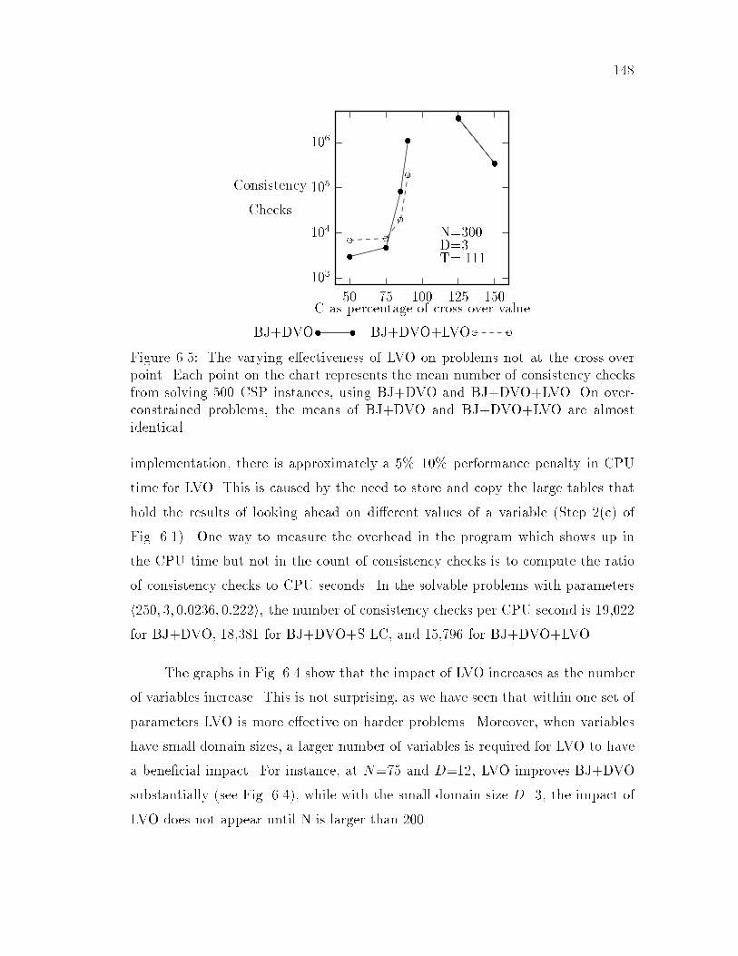
148

Consistency

Checks

C as percentage of cross-over value

BJ+DVO� � BJ+DVO+LVO� �

50 75 100 125 150

103

104

105

106

� �

�

��

�

� ��

� �

�

N=300D=3T=.111

Figure 6.5: The varying e�ectiveness of LVO on problems not at the cross-overpoint. Each point on the chart represents the mean number of consistency checksfrom solving 500 CSP instances, using BJ+DVO and BJ+DVO+LVO. On over-constrained problems, the means of BJ+DVO and BJ+DVO+LVO are almostidentical.

implementation, there is approximately a 5%{10% performance penalty in CPU

time for LVO. This is caused by the need to store and copy the large tables that

hold the results of looking ahead on di�erent values of a variable (Step 2(c) of

Fig. 6.1). One way to measure the overhead in the program which shows up in

the CPU time but not in the count of consistency checks is to compute the ratio

of consistency checks to CPU seconds. In the solvable problems with parameters

h250; 3; 0:0236; 0:222i, the number of consistency checks per CPU second is 19,022

for BJ+DVO, 18,381 for BJ+DVO+S-LC, and 15,796 for BJ+DVO+LVO.

The graphs in Fig. 6.4 show that the impact of LVO increases as the number

of variables increase. This is not surprising, as we have seen that within one set of

parameters LVO is more e�ective on harder problems. Moreover, when variables

have small domain sizes, a larger number of variables is required for LVO to have

a bene�cial impact. For instance, at N=75 and D=12, LVO improves BJ+DVO

substantially (see Fig. 6.4), while with the small domain size D=3, the impact of

LVO does not appear until N is larger than 200.

149

a, b(b,d)

c, d(c,e)

e f, g(g,i)

h, i

X1 X2 X3 X4 X5

(a,f)(a,h)

Figure 6.6: The constraint graph representing a CSP with 5 variables. The domainof each variable is listed inside its oval, and the constraints are indicated by arcs,with the disallowed value pairs noted.

The e�cacy of LVO also depends on how near the parameters are to the 50%

solvable crossover point. As the data in Fig. 6.5 indicate, LVO is detrimental on

very easy underconstrained problems, when C is less than 80% of the cross-over

point value. These problems have many solutions, and the extra work LVO does

exploring all values of a variable is almost always unnecessary. When problems

are su�ciently overconstrained, C greater than 125% of cross-over value, LVO has

very little e�ect on the number of consistency checks, and the points for BJ+DVO

and BJ+DVO+LVO on Fig. 6.5 are indistinguishable.

6.6 LVO and Backjumping

With backtracking the order in which values are chosen does not a�ect the

size of the search space on problems which have no solution, or when searching for

all solutions. Therefore it may be surprising that a value ordering scheme can help

BJ+DVO on instances that are unsatis�able, as the data in Table 6.3 and Fig. 6.3

indicate. Nonetheless, our experiments show that adding LVO to BJ+DVO almost

always changes the number of consistency checks used on unsolvable problems,

often reducing them. One unsolvable instance required 442 million consistency

checks without LVO and 52 million with LVO. As the following observation states,

the reason is the interaction between backjumping and look-ahead value ordering.

Observation 1 When searching for all solutions, or on problems which have no

solution,

150

1. the order in which values are chosen does not a�ect the search space which

backtracking explores;

2. the order in which values are chosen can a�ect the search space which back-

jumping explores.

Proof. Part 1: Consider a search tree rooted at variable X. The n children

of X are X1;X2; . . . ;Xn. The size of the search space SS(X) of this tree is 1 +Pni=1 SS(Xi). Since addition is commutative and the search spaces of the children

do not interact, the order in which the search spaces rooted at the children of X

are expanded will not a�ect SS(X).

Part 2: We will use a simple example; consider the problem depicted in

Fig. 6.6, and assume X1 = a is assigned �rst. There are two value orders for X2. If

X2 = c is considered �rst, then X3 will be a dead-end. X2 = d will be instantiated

next, and an eventual dead-end at X5 will lead to a jump back to X4 and then

to X1. X2 and X3 will be jumped over because they are not connected to X4 or

X5. On the other hand, if X2 = d is considered �rst, a di�erent search space is

explored because X2 = c is never encountered. Instead, X2 and X3 are jumped

over after the dead-ends at X4 and X5.

Note that the observation holds whether a look-ahead or look-back method

is used, and whether the variable ordering is static or dynamic. LVO can help on

unsatis�able problems, and on unsatis�able branches of problems with solutions,

by more quickly �nding a consistent instantiation of a small set of variables which

are later jumped over by backjumping.

6.7 Related Work

In general, domain-independent value ordering schemes have not been con-

sidered e�ective on CSPs, and relatively little work has been done on them. The

151

success of our static least-con icts heuristic was therefore unexpected, and is prob-

ably due to its being evaluated on larger and harder problems than previously used.

This heuristic is similar to the Min-Con icts heuristic developed by Minton et al.

[56], although Minton et al.'s version is not static, and is used primarily for variable

selection.

Geelen [32] describes an approach to value selection similar to ours. It is

based on a forward checking style look-ahead, but does not employ backjumping.

Empirical evaluation in [32] is based on the N-Queens problem.

Pearl [66] discusses similar value ordering heuristics in the context of the

8-Queens problem. His \highest number of unattacked cells" is the same as our

max-con icts heuristic, and his \row with the least number of unattacked cells"

heuristic is the same as max-domain-size.

Dechter and Pearl [18] developed an Advised Backtrack algorithm which

estimates the number of solutions in the subproblem created by instantiating each

value. The estimate is based on a tree-like relaxation of the remainder of the

problem. For each value, the number of solutions is counted, and the count is

used to rank the values. Advised Backtrack was the �rst implementation of the

general idea that heuristics can be generated from a relaxed version of the problem

instance.

Sadeh and Fox [76] also use a tree-like relaxation of the remaining problem,

in the context of job-shop scheduling problems. Their value ordering heuristic con-

siders as well the impact of capacity constraints and demand on scarce resources.

6.8 Conclusions and Future Work

We have introduced look-ahead value ordering, an algorithm for ordering the

values in a constraint satisfaction problem. Our experiments showed that for large

152

and hard problems, LVO could improve the already very good BJ+DVO algorithm

by over a factor of �ve.

We also evaluated a simple static value ordering heuristic called static least-

con icts. Although it is not able to react to changing conditions during search,

this heuristic often was an improvement over plain BJ+DVO.

One drawback of LVO is that it is somewhat complex to implement, as it uses

a set of tables to cache the results of values that have been examined during the

ranking process but not yet instantiated. Manipulating these tables incurs a small

CPU overhead. Another disadvantage of LVO is that on easy solvable problems,

where there are many solutions and hence many acceptable value choices, it is

usually detrimental. LVO needlessly examines every value of each variable along

the almost backtrack-free search for a solution.

LVO is almost always bene�cial on di�cult instances that require over one

million consistency checks. Unexpectedly, it even helps on problems without solu-

tions when used in conjunction with backjumping.

We tested LVO using a forward checking level of look-ahead. It would also

be interesting to explore the possibility that a more computationally expensive

scheme, such as interleaved arc-consistency (see Chapter 5) or directional arc-

consistency [18], will pay o� in the increased accuracy of the value ordering.

Another research direction is to reduce the overhead of LVO on easy problems.

This might be achieved by only employing value ordering in the earlier levels of

the search, or by having value ordering automatically \turn o�" when it notices

that current values are in con ict with relatively few future values, indicating an

underconstrained problem. A simple way to eliminate the overhead of LVO on

very easy problems would be to always run a non-LVO algorithm �rst; if that

algorithm has not completed by, say, 100,000 consistency checks, it is cancelled

and problem solving is restarted with an LVO version. At the price of 100,000

153

extra consistency checks on some di�cult problems, the costs of LVO on the easy

majority of problems would be avoided.

Chapter 7

Dead-end Driven Learning

7.1 Overview of the chapter

This chapter evaluates the e�ectiveness of learning for speeding up the so-

lution of constraint satisfaction problems1. It extends previous work [15] by in-

troducing a new and powerful variant of learning and by presenting an extensive

empirical study on much larger and more di�cult problem instances. Our re-

sults show that the addition of learning can speed up backjumping with dynamic

variable ordering.

7.2 Introduction

Our goal in this chapter is to study the e�ect of learning in speeding up

the solution of constraint problems. Learning has been studied in many branches

of Arti�cial Intelligence. Shavlik and Dietterich [80] distinguish two fundamental

ways in which a computer system can learn: it can \acquire new knowledge from

external sources," which is usually called empirical learning or inductive learning,

or it can \modify itself to exploit its current knowledge more e�ectively." This

latter type of learning is often called speedup learning, and it is into this category

that CSP learning falls.

1This research was �rst reported in Frost and Dechter [26].

154

155

The function of learning in search-based problem solving is to record in a

useful way some information which is explicated during the search, so that it

can be reused either later on the same problem instance, or on similar instances

which arise subsequently. One application of this notion involves the creation of

macro-operators from sequences and subsequences of atomic operators that have

proven useful in solutions to earlier problem instances of the domain. This idea

was exploited in strips with macrops [24, 48]. A more recent approach is to

learn heuristic control rules using explanation-based learning [54, 55].

The approach we take involves a during-search transformation of the problem

representation into one that may be searched more e�ectively. This is done by

enriching the problem description by new constraints, also called nogoods, which

do not change the set of solutions, but make certain information explicit. The new

constraints are essentially uncovered by resolution during the search process [52].

The idea is to learn from dead-ends; whenever a dead-end is reached we record a

constraint explicated by the dead-end. Learning during search has the potential for

reducing the size of the remaining search space, since additional constraints may

cause unfruitful branches of the search to be cut o� at an earlier point. The cost

of learning is that the computational e�ort spent recording and then consulting

the additional constraints may overwhelm the savings. Minton [55] refers to this

trade-o� as the utility problem: \the cumulative bene�ts of applying the knowledge

[additional constraints] must outweigh the cumulative costs of testing whether the

knowledge is applicable." Another potential drawback of the type of learning we

propose with CSPs is that the space complexity can be exponential.

This type of learning has been presented in dependency-directed backtrack-

ing strategies by researchers interested in truth maintenance systems [84], and

within intelligent backtracking for Prolog [9]. It was treated more systematically

by Dechter [15] within the constraint network framework. In [15], di�erent variants

of learning were examined, taking into account the trade-o� between the overhead

156

a, b w, x y, z w, y a, b � � �X1 X2 X3 X4 X5 X6 . . .X10

Figure 7.1: The constraint graph representing a CSP with ten variables. Thedomains of variables X1 through X5 are listed inside the ovals and constraintsare indicated by arcs. Each constraint speci�es that the two variables cannot beassigned the same value.

of learning and performance improvement. The results, although preliminary, indi-

cated that learning during CSP search can be cost-e�ective. The empirical results

in [15] indicate that on randomly generated instances only very restricted forms

of learning paid o�. When experimenting with the Zebra puzzle deeper forms of

learning were quite e�ective; however, instances were solved with random variable

orderings, and it remained unclear whether learning would still be e�ective under

well-chosen orderings. Overall, the empirical evidence to-date is based on a small

number of small-sized instances, under learning that restricts the size of constraints

recorded.

The present study extends [15] in several ways. First, a new variant of

learning, called jump-back learning, is introduced and is shown empirically to be

superior to other types of learning. Secondly, we experiment with and without

restrictions on the size of the constraints learned. Thirdly, we use the highly

e�ective BJ+DVO algorithm from Chapter 4 as a comparison reference. Finally,

our experiments use larger and harder problem instances than previously studied.

Because learning in CSPs operates by recording additional constraints, it is

a variation of constraint propagation. Recall that a CSP is called k-consistent if

every consistent instantiation of k � 1 variables can be extended consistently to

any kth variable. 2-consistency is often called arc-consistency, and 3-consistency is

known as path-consistency. Arc-consistency is enforced by removing values from

157

the domains of variables; higher levels of consistency are enforced by adding con-

straints or tightening existing constraints, so that k � 1 size instantiations which

cannot be consistently extended are themselves prohibited.

A desired level of consistency can be enforced on a CSP before search, or

instead of search. Consistency enforcing can also be interleaved with search (see

Chapter 5). In the latter case, the consistency enforcing algorithm is applied to

a subproblem which results from instantiating a subset of the variables. If one

of these variables is assigned a new value after backtracking, then the results of

the earlier consistency enforcing are out-of-date and must be recalculated. As an

example, consider the small CSP shown in Fig. 7.1, and assume that the problem

has no solution due to the constraints among variables X6 through X10. Enforcing

arc-consistency before search will not change the problem, since in all constrained

pairs of variables each value is compatible with at least one value in the domain

of the other variable. If path-consistency is enforced, a constraint will be added

betweenX2 and X3 which prohibits the assignment (X2=w;X3=y), since with these

values there is no compatible extension to X4. Now let us look at the behavior

of various search algorithms, assuming that the variables are considered in order

of increasing subscript, and the values are selected in alphabetical order. Forward

checking will instantiate (X1=a;X2=w) and upon considering X3=y will discover

an empty domain in X4, therefore rejecting y for X3. Since the variables from X5

on lead to a dead-end, at some point forward checking will return to X1. It will

assignX1=b, thenX2=w, and then again discover that X3=y is not acceptable. The

discovery has to be made twice since it was not remembered when the algorithm

backtracked to X1.

A similar discovery, \forgetting," and re-discovery will happen on this prob-

lem if interleaved arc-consistency (IAC from Chapter 5) is used. Look-ahead al-

gorithms forget when they backtrack, so that what they learn { that particular

values cannot be part of a solution { can be stored with low-order polynomial space

requirements.In Fig. 7.1's example CSP, it might make sense to record that the

158

cause of the dead-end in variable X4 is the combination (X2=w;X3=y). Adding

a constraint prohibiting this combination to the problem's database of constraints

means the dead-end at X4 will not have to be discovered again.

7.3 Backjumping

It will be useful to brie y review the con ict-directed backjumping algorithm,

since the new learning technique we propose is based in part on the mechanics of

backjumping.

When a variable is encountered such that none of its possible values is con-

sistent with previous assignments, a dead-end occurs and a backjump takes place.

The idea is to jump back over several irrelevant variables to a variable which is

more directly responsible for the current con ict. The backjumping algorithm

identi�es a parent set, that is, a subset of the variables preceding the dead-end

variable which are inconsistent with all its values, and continues search from the

last variable in this set. If that variable has no untried values left, then a interior

dead-end arises and further backjumping occurs.

Consider, for instance, the CSP represented by the graph in Fig. 7.3. Each

node represents a variable that can take on a value from within the oval, and

the binary constraint between connected variables is speci�ed along the arcs by

the disallowed value pairs. If the variables are ordered (X1;X5;X2;X3;X4) and a

dead-end is reached at X4, the backjumping algorithm will jump back to X5, since

X4 is not connected to X3 or X2.

159

7.4 Learning Algorithms

Upon a dead-end at Xi, when the current instantiation S=(X1=x1; . . . ;Xi�1=

xi�1) cannot be extended by any value of Xi, we say that S is a con ict set. Note

that when using a look-ahead approach, as BJ+DVO does, Xi may be any future,

uninstantiated, variable, and a dead-end at Xi means that the domain D0i has

become empty. An opportunity to learn new constraints is presented whenever

backjumping encounters a dead-end, since had the problem included an explicit

constraint prohibiting the dead-end's con ict-set, the dead-end would have been

avoided. To learn at a dead-end, we record one or more new constraints which

make explicit an incompatibility among variable assignments that already existed,

implicitly.

There is no point in recording S as a constraint at this stage, because under

the backtracking control strategy this state will not recur. However, if S contains

one or more subsets that are also in con ict with Xi, then recording these smaller

con ict sets as constraints may prove useful in the continued exploration of the

search space.

Varieties of learning di�er in the way they identify smaller con ict sets. In

[15] learning is characterized as being either deep or shallow. Deep learning only

records minimal con ict sets, that is, those that do not have subsets which are also

con ict sets. Shallow learning allows non-minimal con ict sets to be recorded as

well. Non-minimal con ict sets are easier to discover, but may be more expensive

to store and applicable less frequently in the remaining search.

Learning can also be characterized by order, the maximum constraint size

that is recorded. In [15] experiments were limited to recording unary and binary

constraints, or �rst and second order learning. A loose upper-bound on the space

complexity of i-th order learning is (nd)i, where n is the number of variables and

d is the largest domain size.

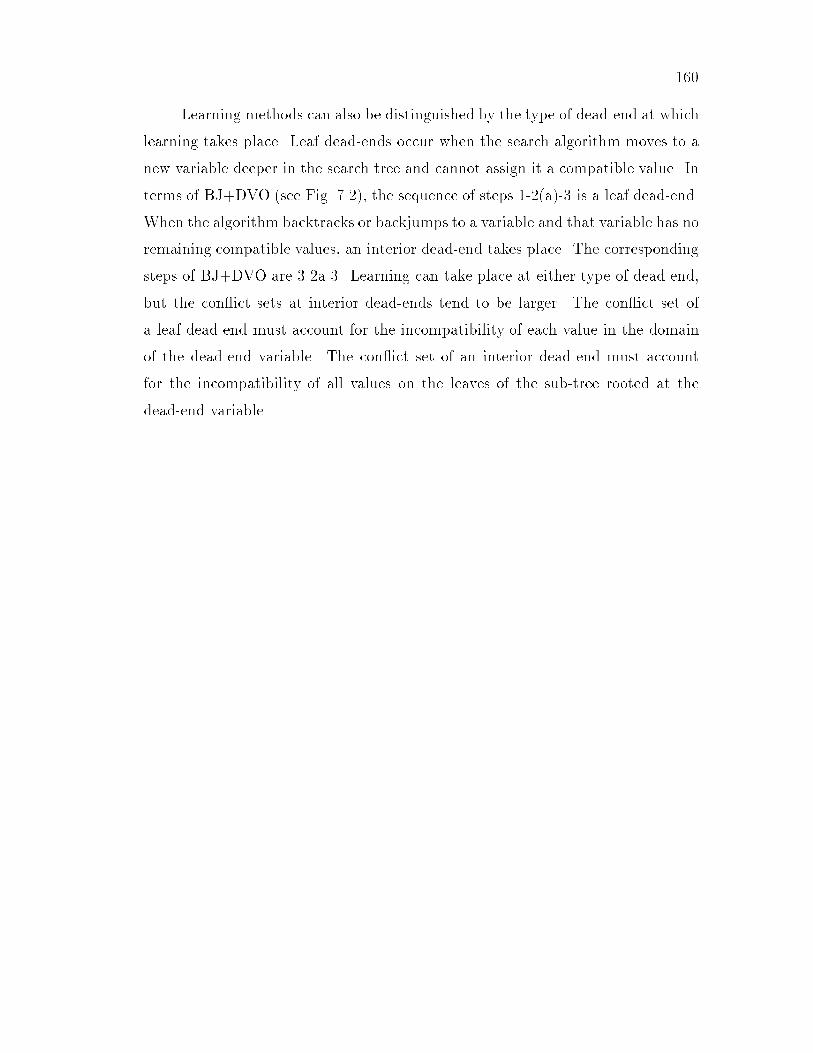
160

Learning methods can also be distinguished by the type of dead-end at which

learning takes place. Leaf dead-ends occur when the search algorithm moves to a

new variable deeper in the search tree and cannot assign it a compatible value. In

terms of BJ+DVO (see Fig. 7.2), the sequence of steps 1-2(a)-3 is a leaf dead-end.

When the algorithm backtracks or backjumps to a variable and that variable has no

remaining compatible values, an interior dead-end takes place. The corresponding

steps of BJ+DVO are 3-2a-3. Learning can take place at either type of dead-end,

but the con ict sets at interior dead-ends tend to be larger. The con ict set of

a leaf dead-end must account for the incompatibility of each value in the domain

of the dead-end variable. The con ict set of an interior dead-end must account

for the incompatibility of all values on the leaves of the sub-tree rooted at the

dead-end variable.

161

Backjumping with DVOInput: type, order, leaf-only

0. (Initialize.) Set D0i Di for 1 � i � n.

1. (Step forward.) If Xcur is the last variable, then all variables have valueassignments; exit with this solution. Otherwise, set cur to be the indexof the next variable, according to a variable-ordering-heuristic.Set Pcur ;.

2. Select a value x 2 D0cur. Do this as follows:

(a) If D0cur = ;, go to 3.

(b) Pop x from D0cur and instantiate Xcur x.

(c) Examine the future variables Xi; cur < i � n. For each v in D0i, if

Xi = v con icts with ~xcur then remove v from D0i and add Xcur to

Pi; if D0i becomes empty, go to (d) (without examining other Xi's).

(d) Go to 1.

3. Learn, then backjump.

(a) If Pcur = ; (there is no previous variable), exit with \inconsistent."

(b) If leaf-only = true and Xcur was reached by a backjump, go to (g).

(c) If type = VALUE, perform value-based-learning(order);

(d) else if type = GRAPH, perform graph-based-learning(order);

(e) else if type = DEEP, perform deep-learning(order);

(f) else if type = JUMP, perform jump-back-learning(order).

(g) Set P Pcur; set cur equal to the index of the last variable in P .Set Pcur Pcur [ P � fXcurg. Reset all D0 sets to the way theywere before Xcur was last instantiated. Go to 2.

Figure 7.2: The BJ+DVO algorithm, augmented to call a learning procedure.

162

x,y,z

X5

a,b,c

X1

a,b,c

X2

a,b,cX3a,b,cX4

(a,x),(a,y) (b,z)

(a,x)(c,z)

Figure 7.3: A small CSP. Note that the disallowed value pairs are shown on eacharc.

We experimented with four types of learning. Three were proposed by

Dechter [15]: graph-based shallow learning, value-based shallow learning (called

full shallow learning in [15]), and deep learning. We introduce a new variety of

learning, called jump-back learning because of its reliance on backjumping's parent

or \jump-back" set of variables. As described below, each learning algorithm re-

lies on a subprocedure record to add a new constraint or nogood to the problem

representation. (We do not de�ne record, because it relies on the speci�c data

structures used in the computer program.) In general, graph-based learning records

the largest new constraints, and deep learning the smallest. Value-based learning

and jump-back learning are intermediate forms that take di�erent approaches to

the tradeo� between minimizing the cost at each dead-end and learning useful

constraints.

7.4.1 Value-based learning

In value-based learning, which is described in Fig. 7.4, all irrelevant variable-

value pairs are removed from the initial con ict set S. If a variable-value pair Xj=

xj does not con ict with any value of the dead-end variable then it is redundant and

can be eliminated. For instance, if we try to solve the problem in Fig. 7.3 with the

ordering (X1;X2;X3;X4;X5), after instantiating X1=a;X2=b;X3=b;X4=c, the

dead-end at X5 will cause value-based learning to record (X1= a;X2= b;X4= c),

163

value-based-learning(order)1 CS ; ; initialize con ict-set2 for each instantiated variable Xi=xi; 1 � i � cur,3 if Xi=xi con icts with some value of Xcur

4 then add Xi=xi to CS5 if size of CS � order6 then record(CS)

Figure 7.4: The value-based learning procedure.

since the pair X3 = b is compatible with all values of X5. If all constraints in a

CSP are binary, a three-dimensional table CONF of boolean values can be pre-

computed before search. CONFi;j;k is true if Xi=xj is in con ict with any value

of Xk, and false otherwise. Creating this table requires O(n2d) space and time

complexity. Since there are at most n�1 variable preceeding the dead-end variable,by consulting CONF the time complexity of value-based learning at each dead-end

is O(n).

If the CSP has non-binary constraints, the same look-up table can be em-

ployed, but CONFi;j;k = true will mean that Xi=xj in combination with some

other variables is in con ict with at least one value of Xk. This approach main-

tains the e�cient preprocessing requirement and the O(n) time complexity per

dead-end, but is undesirable because some variables will be retained in the con ict

set unnecessarily. The alternatives are to construct a larger table in advance, or

to do more extensive analysis of the con ict set at each dead-end, which will take

more time.

7.4.2 Graph-based learning

Graph-based shallow learning is a relaxed version of value-based learning,

where information on con icts is derived from the constraint graph alone, without

consulting the values currently assigned to variables (see Fig. 7.5). This approach

may be particularly useful on sparse graphs. For instance, when applied to the CSP

164

graph-based-learning(order)1 CS ;2 for each instantiated variable Xi; 1 � i � cur,3 if there exists a constraint between Xi and Xcur

4 then add Xi=xi to CS5 if size of CS � order6 then record(CS)

Figure 7.5: The graph-based learning procedure.

in Fig. 7.3, graph-based shallow learning might record (X1=a;X2=b;X3=b;X4=c)

as a con ict set relative to a dead-end at X5, since these variables are connected to

X5. The complexity of learning at each dead-end here is O(n), since each variable

is connected to at most n � 1 other variables.

7.4.3 Jump-back learning

Jump-back learning uses as its con ict-set the parent set P that is explicated

by the backjumping algorithm itself. Recall that BJ+DVO examines each future

variable Xi and includes Xcur in the parent set Pi if Xcur, as instantiated, con icts

with a value of Pi that previously did not con ict with any variable. For instance

in Fig. 7.3, when using the same ordering and reaching the dead-end at X5, jump-

back learning will record (X1=a;X2=b) as a new constraint. These two variables

are selected because the algorithm �rst looks at X1=a and, noting that it con icts

with X5=x and X5=y, adds X1 to P5. Proceeding to X2=b, the con ict with X5=z

is noted and X2 is added to P5. At this point all values of X5 have been ruled

out, and the con ict set is complete. Since the con ict set needed for learning is

jump-back-learning(order)1 CS Pcur2 if size of CS � order3 then record(CS)

Figure 7.6: The jump-back learning procedure.

165

deep-learning(order)1 for each subset S of the instantiated variables ~xcur�1,2 in order from smallest to largest,3 if every value of Xcur is in con ict with S and4 S is not a superset of any existing nogood,5 then if size of CS � order6 then record(CS)

Figure 7.7: The deep learning procedure.

already assembled by the underlying backjumping algorithm, the added complexity

of computing the con ict set is constant. To achieve constant time complexity at

each dead-end the parent set must be modi�ed to include not only the parent

variables but also their current values.

The con ict set identi�ed by backjumping is not necessarilyminimal. Refering

to the problem in Fig. 7.3, if the variable ordering starts with (X1;X2), then the

dead-end at X5 will result in the minimal con ict set (X1=a;X2=b), as discussed

in the previous paragraph. But if the variable ordering is (X3;X1;X2), then the

parent set for X5 will be (X3=a;X1=a;X2=b), which is not a minimal con ict set.

7.4.4 Deep learning

In deep learning all and only minimal con ict sets are recorded. With the

CSP in Fig. 7.3, a dead-end at X5 will cause deep learning will record two minimal

con ict sets, (X1=a;X2=b) and (X1=a;X4=c). The deep learning algorithm can

start with the value-based con ict set, generate its subsets and test whether they

are con ict sets. Although this form of learning is the most accurate, its cost is

prohibitive and in the worst-case is exponential in the size of the initial con ict

set. As noted in [15], if r is the cardinality of the starting con ict set, we can

envision a worst case where all the subsets of this set having r=2 elements are in

166

Parameters Algorithm CC Nodes CPU Sizeh125; 3; 0:1199; 0:111i None 242,293 8,760 2.02

Graph 1,253,404 8,692 15.73 3.6Value 619,059 8,000 5.19 3.3Jump 518,454 7,828 3.14 3.3Deep 2,067,166 7,183 10.17 3.2

h175; 3; 0:0358; 0:222i None 72,289 6,221 2.01Graph 785,564 6,201 8.32 3.5Value 398,451 5,163 3.86 3.0Jump 26,637 2,008 0.56 2.5Deep 823,306 1,299 4.17 2.1

h150; 3; 0:0218; 0:333i None 5,120 749 0.22Graph 112,674 579 3.01 2.3Value 84,711 571 0.91 1.9Jump 1,332 188 0.07 1.8Deep 57,881 165 0.54 1.5

Table 7.1: Comparison of BJ+DVO, without learning (\None") and with four vari-eties of learning: Graph-based learning (\Graph"), Value-based learning (\Value"),Jump-back learning (\Jump"), and Deep Learning (\Deep"). All learning was re-stricted to 4th-order. Each number is the mean of 500 solvable and unsolvableinstances. The \Size" column displays the average number of variables in thelearned constraints.

con ict with Xcur. The number of minimal con ict sets will then be:

#min-con ict-sets =

0B@ r

r=2

1CA �= 2r;

which amounts to exponential time and space complexity at each dead-end.

7.5 Experimental Results

We evaluated the learning algorithms by combining them with BJ+DVO and

solving several sets of random CSPs. The results are presented in the following

subsections.

167

7.5.1 Comparing learning algorithms

The �rst experiment was designed to compare the e�ectiveness of the four

learning schemes. Fig. 7.1 presents a summary of experiments with problems

generated from three sets of parameters. 500 problems in each sets were generated

and solved by �ve algorithms: BJ+DVO without learning, and then BJ+DVO

with each of the four types of learning. In all cases a bound of four was placed on

the size of the constraints recorded, and learning was limited to leaf dead-ends.

Looking at the size of the search space, the results reported in Fig. 7.1 indicate

that the algorithms can be ranked as follows: no learning > Graph-based > Value-

based > Jump-back > Deep. This result is expected: learning adds additional

constraints which should reduce the size of the search space. Within the learning

schemes, the size of the search space is inversely related to the average size of

the learned constraints, since larger constraints tend to be less e�ective in the

remainder of the search.

Because learning adds new constraints, it can increase the number of consis-

tency checks performed later in the search. Moreover, learning applied to binary

CSPs can add constraints with more than two variables, and these constraints can

be more expensive to query2. Deep learning makes a particularly large number of

consistency checks because at each dead-end it has to verify whether each subset

of the value-based con ict set is a minimal con ict set.

This experiment demonstrates that only the new jump-back type of learning

is e�ective on these reasonably large size problems. In the following discussion and

�gures, all references to learning should be taken to mean jump-back learning.

2In our implementation, binary constraints are represented by a four-dimensional array with

one dimension for each variable and value, and a binary consistency check is therefore a constant

time operation. Higher order constraints are stored in ordered lists, and checking consistency

with one of these constraints is proportional to r � log s, where r is the size of the constraint,

and s is the number of high-order constraints.

168

� � cons. chks.� � nodes? ? CPU� � avg. size� � num learned

No 2 3 4 5 6 7 8 9

6,248K� � � � ��

�

�

�193,000K

294K �

� � � � � �

� � 151K47.76 ?

? ? ? ? ?

? ?

? 96.05

2.0 �� �

����� 7.0

41 ��

�

�

�

�

�

� 1,461

Figure 7.8: Results from experiments with parameters h100; 6; :0772; :333i andvarying orders of jump-back learning, as indicated on the x-axis (\No" signi�esBJ+DVO without learning). Note that each statistic is on a di�erent scale.

7.5.2 Testing i-th order learning

We now describe a set of experiments designed to investigate the impact on

learning of restricting the size of the learned constraints. Recall that in ith-order

learning, new constraints are recorded only if they include i or fewer variables. The

experiments used random problems generated with parameters h100; 6; :0772; :333i(reported in Fig. 7.8) and h125; 6; :0395; :444i (reported in Fig. 7.9). For both ex-

periments we generated 500 instances and processed them using BJ+DVO without

learning, and using BJ+DVO with i-th order learning, where i ranged from 2 to

9. The graphs in the �gures show the averages for number of consistency checks,

the size of the search space, the CPU time in seconds, the number of constraints

learned, and the size of the learned constraints. Each set of �gures is plotted using

a di�erent y-axis scale, with the beginning and ending values indicated on the

charts. In general, a higher order of learning results in a smaller search space,

a larger number of learned constraints, and a larger average size of the learned

169

� � cons. chks.� � nodes? ? CPU� � avg. size� � num learned

No 2 3 4 5 6 7 8 9

3,527K�� � � � �

�

�

� 25,583K

239K �

� � � � � � � � 77K

47.60 ?

?

?

?? ? ? ?

? 27.65

1.9 � � � � � � �� 5.8

86 ��

�

�

�

�

�

� 698

Figure 7.9: Results from experiments with parameters h125; 6; :0395; :444i andvarying orders of jump-back learning, as indicated on the x-axis. \No" signi�esBJ+DVO without learning. Note that each statistic is on a di�erent scale.

constraints. Although this relationship usually holds true on average, it is not nec-

essarily the case on an instance by instance basis, since new constraints a�ect the

dynamic variable ordering and occasionally produces a worse ordering. Charting

the CPU time and number of consistency checks produces a U-shaped curve in

respect to the learning order: a low order (2 { 4 for the problems with T=:333 and

2 { 8 for the problems with T=:444) reduces the average CPU time required, but

if the order of learning is too high learning impairs the performance of BJ+DVO.

This pattern holds true on many other sets of data we have examined: learning

is best when limited. When the constraints are tighter in the original CSP, the

optimum order of learning is higher. The problems with T=:444 in Fig. 7.9 are

solved with in 23.23 CPU seconds, on average, with 8th-order learning, although

this is perhaps negligibly lower than 24.40 CPU seconds with 2nd-order learning.

When the constraints are quite loose, the order of learning can have little

e�ect. For example, on problems with D=3 and T=:111=1=9 almost all learned

170

constraints have exactly 3 variables, since each of the three values of the dead-

end variable is incompatible with a di�erent previous variable. After non-binary

constraints are added to the problem, it is possible for a dead-end to have a con ict

set of more or less than 3 variables. Thus 2nd-order learning on such problems

results in no learning, while learning without an order restriction is almost identical

to 3rd-order learning.

7.5.3 Increasing the number of variables

Learning tends to have a greater impact on harder problems; an easy problem

with relatively few dead-ends presents few opportunities for learning to come into

play. To verify that learning is more bene�cial on larger problems, we ran an

experiment on six sets of random problems, where the number of variables varied

from 50 in the �rst set to 300 in the sixth. The results are reported in Fig. 7.10.

Only data from unsolvable problems is included so that estimates of the lognormal

distribution's � and � parameters can be shown (see Chapter 3), but the growth

in mean consistency checks for solvable problems is similar.

171

� log(mean) BJ+DVO+lrn./ log(mean) BJ+DVO� � BJ+DVO+learning? � BJ+DVO� � BJ+DVO+learning� � BJ+DVO

50 100 150 200 250 300N

5

6

7

8

9

10

11

12

13

14

15

�

�

�

�

�

�

�

./

./

./

./

./

./

�

�

�

��

� 0:0192N + 6:3944

?

?

?

?

?

? 0:0252N + 6:1138

0

.5

1.0

1.5

2.0

�

� �� � � � 0:0034N + :3753

��

� � � � 0:0042N + :4177

Figure 7.10: Data on number of consistency checks required on unsolvable problemsin experiments with parameters D=3, T=:222, N varying from 50 to 300, and Cset to the cross-over point, using BJ+DVO with and without 4th-order learning.Points represent estimated � (left hand scale) and � (right hand scale) for eachalgorithm, assuming a lognormal distribution. Lines (solid for BJ+DVO withlearning, dotted for BJ+DVO without) show best linear �t. The formula to theright of each line shows the slope and the y-axis intercept. The graph also showsthe natural logarithm of the mean number of consistency checks (left hand scale).

172

Mean CPU seconds

Decile No learning Learning Ratio

1 951.09 67.46 14.10

2 333.70 52.22 6.39

3 159.94 27.72 5.77

4 100.43 19.70 5.10

5 65.92 7.76 8.49

6 43.35 5.85 7.41

7 28.63 5.17 5.54

8 12.55 2.38 5.27

9 6.30 1.35 4.66

10 1.57 0.56 2.79

Figure 7.11: Results from experiments comparing BJ+DVO with and withoutlearning on random instances with parameters h300; 2; :0089; :333i. Mean CPUtime for each decile of the data is reported.

The results in Fig. 7.10 are similar to those in Fig. 4.12 from Chapter 4. The

presence of learning slows the growth in both � and �, so that the distribution

of BJ+DVO is less skewed with learning than without. Fig. 7.11 shows the CPU

times from the largest set of problems in Fig. 7.10, those with N =300. The

500 instances, both solvable and unsolvable, have been divided into 10 groups of

50, based on the CPU time required by BJ+DVO without learning to solve each

instance. The hardest 50 were put in the �rst group, the next hardest in the second

group, and so on. On the hardest instances, the improvement due to learning was

a factor of 14; for the easiest 50 problems learning still helps, but only by a factor

of about three. As expected, learning is more e�ective on problem instances that

have more dead-ends and larger search spaces, where there are more opportunities

for each learned constraint to be useful.

173

No learning� � Fourth-order learning� �

CPU seconds

number of constraints1,100 1,300 1,800 2,000 2,200

:1

1

10

100

1000

� � � �

��

��

�� �

� � � � � �

� � � �

�

�� �

� � � � � � � �

Figure 7.12: BJ+DVO without learning and with third-order learning, for N=500,D=3, T=:222, and non-crossover point values of C. All problems with fewer than1,350 constraints were solvable; all problems with more than 1,800 had no solution.

7.5.4 Problems not at the cross-over point

Fig. 7.12 shows that with large enough N , problems do not have to be drawn

from the 50% satis�able area in order to be hard enough for learning to help. We

experimented with problems not at the cross-over point by setting N=500, D=3,

T=:222, and selecting values of C that are larger or smaller than the estimated

cross-over point of .0123 (1,534 constraints). 250 instances were generated with

each set of parameters. Learning was especially valuable on extremely hard solvable

problems generated by slightly underconstrained values for C. For instance, at

h500; 3; :0100; :222i, the hardest problem took 47 CPU hours without learning,

and under one CPU minute with learning. The next four hardest problems took

4% as much CPU time with learning as without.

174

7.6 Average-case Space Requirements

It is worth noting that we did not �nd the space requirements of learning to be

overwhelming, as has been reported by some researchers. For instance, even with

a learning order of 9, only 698 constraints were learned, on average, for reasonably

hard problems with parameters h125; 6; :0395; :444i (see Fig. 7.9). On the hardest

problem in the set, which took 86 CPU minutes and made over two and a half

billion consistency checks, 10,524 new constraints were added, with an average

size of 7.37. Allowing 500 bytes to store such a large constraint and index it by

each included variable-value pair, the run-time addition to computer memory is

about �ve megabytes. Such an amount is not trivial, but does not pose a problem

for modern computer systems. Furthermore, the order of learning can be limited

to control the space used, if necessary. We have found that computer memory is

not the limiting factor; time is.

7.7 Conclusions

We have introduced a new variant of learning, called jump-back learning,

which is more powerful than previous versions because it takes advantage of pro-

cessing already performed by the con ict-directed backjumping algorithm. Our

experiments show that it is very e�ective when augmented on top of the strong

BJ+DVO version of backjumping, resulting in at least an order of magnitude re-

duction in CPU time for some problems.

Learning seems to be particularly e�ective when applied to instances that are

large or hard, since it requires many dead-ends to be able to augment the initial

problem in a signi�cant way. However, on easy problems with few dead-ends,

learning will add little if any cost, thus perhaps making it particularly suitable for

situations in which there is a wide variation in the hardness of individual problems.

In this way learning is superior to other CSP techniques which modify the initial

175

problem, such as by enforcing a certain order of consistency, since the cost will not

be incurred on very easy problems.

An important parameter when applying learning is the order, or maximum

size of the constraints learned. With no restriction on the order, it is possible to

learn very large constraints that will be unlikely to prune the remaining search

space.

Chapter 8

Comparison and Synthesis

8.1 Overview of Chapter

The previous chapters have described and evaluated a number of CSP al-

gorithms. Each was shown to have interesting properties and to be useful on

certain problems. This chapter reports several experiments designed to draw to-

gether the earlier results into a single coherent picture. BT+DVO, BJ+DVO,

BT+DVO+IAC, BJ+DVO+LVO, and BJ+DVO+Learning are compared on both

random problems and on a suite of problems from the Second DIMACS Implemen-

tation Challenge. We also introduce a new algorithms, BJ+DVO+LRN+LVO,

which adds both jump-back learning and look-ahead value ordering to BJ+DVO.

8.2 Combining Learning and LVO

The look-ahead value ordering heuristic from Chapter 6 tentatively instanti-

ates each value of the current variable and uses forward checking style look-ahead

to gauge the value's impact on the remaining search space. The jump-back learn-

ing algorithm described in Chapter 7 records as constraints the con ict sets built

by con ict-directed backjumping and used when a dead-end is encountered. These

two orthogonal improvements to the BJ+DVO algorithm can be combined into a

176

177

single algorithm, which we call BJ+DVO+LRN+LVO. The algorithm is described

in Fig. 8.1.

BJ+DVO+LRN+LVO is modeled on BJ+DVO+LVO. The primary di�er-

ence lies in step 1A (b). In learning algorithms without LVO, an opportunity to

learn occurs at each dead-end. In the presence of LVO, the algorithm can learn

a new nogood for each value of the current variable which will lead to a dead-

end. For instance, suppose the current variable X50 has three values in its domain,

fa; b; cg. The LVO mechanism in step 1A records the impact that X50=a, X50=b,

and X50=c, each have on future variable domains. If it happens that each value

causes a future domain to be empty, then three nogoods will be recorded, di�ering

only in their value for X50.

8.3 Experiments on Large Random Problems

The �rst set of experiments reported in this chapter were based on the same

Model B random problem generator used elsewhere in this thesis. Because the best

algorithms from earlier chapters are compared in this experiment, it was possible

to test them on larger problems than previously reported. We brie y review the

algorithms compared in this chapter:

� BT+DVO. Backtracking with a dynamic variable ordering heuristic.

� BT+DVO+IAC. Backtracking with a dynamic variable ordering heuristic

and arc-consistency performed after each instantiation. Arc-consistency is

achieved by the ac-3 algorithm, using the ac-dc domain checking technique

described in Chapter 4.

� BJ+DVO.Con ict-directed backjumping with a forward checking look-ahead

and dynamic variable ordering.

� BJ+DVO+LVO. The BJ+DVO algorithm with the look-ahead value order-

ing heuristic described in Chapter 5.

178

Backjumping with DVO and Learning and LVOInput: order

0. (Initialize.) Set D0i Di for 1 � i � n.

1. (Step forward.) If Xcur is the last variable, then all variables have valueassignments; exit with this solution. Otherwise, set cur to be the indexof the next variable, determined according to avariable-ordering-heuristic. Set Pcur ;.

1A. (Look-ahead value ordering.) Rank the values in D0cur as follows:

(a) For each value x in D0cur , and for each value v of a future variables

Xi; cur < i � n, determine the consistency of(~xcur�1;Xcur=x;Xi=v).

(b) If instantiating a value x leads to an empty domain of some futurevariable Xf , then add Xcur=x to Pf and learn by recording Pf as anew constraint, unless its size is greater than order.

(c) Using a heuristic function, compute the rank of x based on thenumber and distribution of con icts with future values v.

2. Select a value x 2 D0cur. Do this as follows:

(a) If D0cur = ;, go to 3.

(b) Pop the highest ranked value x from D0cur and instantiate Xcur x.

(c) (This step can be avoided by caching the results from step 1A.)Examine the future variables Xi; cur < i � n. For each v in D0

i, ifXi = v con icts with ~xcur then remove v from D`i and add Xcur toPi; if D0

i becomes empty, go to (d) (without examining other Xi's).

(d) Go to 1.

3. (Backjump.) If Pcur = ; (there is no previous variable), exit with\inconsistent." Otherwise, set P Pcur; set cur equal to the index ofthe last variable in P . Set Pcur Pcur [ P �fXcurg. Reset all D0 sets tothe way they were before Xcur was last instantiated. Go to 2.

Figure 8.1: Algorithm BJ+DVO+LRN+LVO, which combines backjumping, dy-namic variable ordering, jump-back learning, and look-ahead value ordering.

179

Parameters Algorithm CC Nodes CPUh200; 3; 0:0592; 0:111i BT+DVO 5,871,215 207,183 68.46

BT+DVO+IAC 23,836,368 40,098 55.44BJ+DVO 5,365,467 188,726 69.28BJ+DVO+LVO 4,793,417 167,211 73.78BJ+DVO+LRN 5,731,244 186,582 63.39BJ+DVO+LRN+LVO 5,622,825 159,739 74.00

h300; 3; 0:0206; 0:222i BT+DVO+IAC 141,606 632 0.65BJ+DVO 2,483,520 222,285 119.26BJ+DVO+LVO 1,623,455 131,593 86.76BJ+DVO+LRN 419,193 32,221 15.62BJ+DVO+LRN+LVO 392,606 25,771 13.98

h350; 3; 0:0089; 0:333i BT+DVO+IAC 24,641 494 0.43BJ+DVO 1,238,479 182,328 140.81BJ+DVO+LVO 969,224 118,854 111.79BJ+DVO+LRN 3,727 464 0.46BJ+DVO+LRN+LVO 22,688 1,036 3.78

Table 8.1: Comparison of �ve algorithms on random CSPs with D=3. Eachnumber is the mean of 2,000 solvable and unsolvable instances. The algorithmwith the lowest mean CPU seconds in each group is in boldface.

� BJ+DVO+LRN. BJ+DVOwith jump-back learning, as de�ned in Chapter 7.

Only nogoods with four or fewer variables are learned, and learning is only

performed at leaf dead-ends.

� BJ+DVO+LRN+LVO. BJ+DVO with fourth-order jump-back learning and

look-ahead value ordering, as described in the previous section.

Various combinations of parameters N , D, C, and T , were selected, all near

the cross-over region where 50% of the problem have solutions. For each set of

parameters were generated 2,000 instances and applied the algorithms to each in-

stance. Experiments reported in Chapter 4 demonstrated that on large problems

with tight constraints, BT+DVO does not perform well. We therefore applied that

algorithm only to problems with relatively loose constraints, speci�cally parameter

combinations h200; 3; 0:0592; 0:111i, h60; 6; 0:4797; 0:111i, and h75; 6; 0:1744; 0:222i.The results of the experiments are reported in Table 8.1 and Table 8.2.

180

Parameters Algorithm CC Nodes CPUh60; 6; 0:4797; 0:111i BT+DVO 24,503,115 412,494 59.72

BT+DVO+IAC 104,319,923 65,432 130.54BJ+DVO 24,228,726 407,253 63.10BJ+DVO+LVO 23,904,430 401,131 66.47BJ+DVO+LRN 24,368,062 406,332 57.43BJ+DVO+LRN+LVO 24,103,544 405,899 65.75

h75; 6; 0:1744; 0:222i BT+DVO 7,766,594 249,603 40.77BT+DVO+IAC 18,419,580 16,395 22.22BJ+DVO 7,530,726 241,124 42.67BJ+DVO+LVO 7,228,548 230,073 44.05BJ+DVO+LRN 7,856,321 230,367 42.13BJ+DVO+LRN+LVO 7,321,890 231,455 43.79

h100; 6; 0:0772; 0:333i BT+DVO+IAC 4,718,685 4,625 5.67BJ+DVO 6,248,608 293,922 67.30BJ+DVO+LVO 6,581,314 305,121 76.49BJ+DVO+LRN 5,979,767 232,780 54.34BJ+DVO+LRN+LVO 6,034,538 235,509 61.22

h125; 6; 0:0395; 0:444i BT+DVO+IAC 479,228 566 0.60BJ+DVO 3,526,619 238,584 66.17BJ+DVO+LVO 3,007,791 195,720 62.54BJ+DVO+LRN 2,050,232 108,482 28.80BJ+DVO+LRN+LVO 1,970,645 102,788 29.45

h150; 6; 0:0209; 0:555i BT+DVO+IAC 32,537 111 0.06BJ+DVO 3,253,255 359,095 111.70BJ+DVO+LVO 1,328,189 124,415 47.08BJ+DVO+LRN 339,191 28,056 8.25BJ+DVO+LRN+LVO 601,454 25,769 12.87

Table 8.2: Comparison of �ve algorithms on random problems with D=6. Eachnumber is the mean of 2,000 solvable and unsolvable instances. The algorithmwith the lowest mean CPU seconds in each group is in boldface.

181

We also present graphically some of the data from Tables 8.1 and 8.2, which

permits more information than just averages to be conveyed. Fig. 8.2 shows the

distribution of consistency checks made and nodes expanded for three algorithms

on unsatis�able problems with parameters h350; 3; 0:0089; 0:333i. The distribu-

tions are approximated by lognormal curves with estimated � and � parame-

ters. Fig. 8.3 is a scatter chart, in which each point indicates the relative per-

formance of BT+DVO+IAC and BJ+DVO+LRN on a problem with parameters

h75; 6; 0:1744; 0:222i.

8.4 Experiments with DIMACS Problems

The Second Dimacs Implementation Challenge in 1993 [44] collected a set

of satis�ability problem instances for the purpose of providing benchmarks for

comparison of algorithms and heuristics. We compared our algorithms against six

of the problems that were derived from circuit fault analysis. The problems are

encoded as Boolean satis�ability problems in conjunctive normal form. Clauses

contain from one to six variables.

Each of our six algorithms was applied to these benchmark problems. The

results are displayed in Table 8.3 and Table 8.4. The tables show other CPU times

on these problems reported in [44]. Dubois et al. [21] uses a complete algorithm

based on the Davis-Putnam procedure; computer is a Sun SparcStation 10 model

40. Hampson and Kibler [39] use a randomized hill climbing procedure; computer

is a Sun SparcStation II. Jaumard et al. [43] use a complete Davis-Putnam based

algorithm with a tabu search heuristic; computer is a Sun SparcStation 10 model

30. Pretolani's H2R algorithm [67] is based on the Davis-Putnam procedure and

uses a pruning heuristic; computer is a Sun SparcStation 2. Resende and Feo

[72] present a greedy randomized adaptive search procedure called GRASP-A; the

computer used was not reported. Spears [83] uses a simulated annealing based

algorithm; computer is a Sun SparcStation 10. Van Gelder and Tsuji [87] use

182

h350; 3; 0:0089; 0:333iBT+DVO+IAC: �=9:09 �=1:45BJ+DVO+LRN: �=7:77 �=1:18BJ+DVO+LRN+LVO: �=9:55 �=1:16

0 5,000 10,000 15,000Consistency Checks

Frequency

.01

.02

IAC

LRN

LRN+LVO

h350; 3; 0:0089; 0:333iBT+DVO+IAC: �=4:00 �=2:07BJ+DVO+LRN: �=5:42 �=1:29BJ+DVO+LRN+LVO: �=5:98 �=1:28

0 250 500 750Nodes

Frequency

.02

.04

.06

.08

.10

.12

IAC

LRN

LRN+LVO

Figure 8.2: Lognormal curves based on unsolvable problems generated from pa-rameters h350; 3; 0:0089; 0:333i. The top graph is based on consistency checks, thebottom graph on search space nodes. � and � parameters were estimated usingthe Maximum Likelihood Estimator (see Chapter 3).

183

CPU seconds

- BJ+DVO+LRN

Consistency Checks - BT+DVO+IAC0 25 50 75 100 125

0

25

50

75

100

125

���

���

�������

���

��������

�

�

��

�

�

�

�� ��

�

�������

��

��

�

�����

�����

��

�

��

�

��

��

�

�����

�

� ���

��

���

�

����������

���

�

�

�����

�����

�

���������

�

�

�����

�

��

�

��

���

�

�

�������

���

������

����

��

�����

��

� �

��

� �� ���

�

�

�

��

�

������� ���

��

������

���

����

���

��

�

� �

�

�

�

�

������������

��

�

��

��

�

�

�

�����

�� ���

�����

�

�

�

��

��

�����

�

�����

�����

����������������

�����

�����

������

�����

�����

�����

������

�����������

���

���

���

������

�

���

�

�

�

�����

�

��

��

��

��������

������

Figure 8.3: Each point (� = has solution, � = no solution) represents one instancefrom the experiment with h75; 6; 0:1744; 0:222i. Points above the diagonal linerequired less CPU time with BT+DVO+IAC than with BJ+DVO+LRN.

a complete algorithm that combines search and resolution; computer is a Sun

SparcStation 10 model 41.

Among our six algorithms, no clear trend is discernible. BT+DVO+IAC had

the best CPU time on three problems, including one tie with BJ+DVO+LRN,

and BJ+DVO+LRN was best on two, including the tie. BJ+DVO+LVO and

BJ+LVO+LRN+LVO were each best one on problem. On the hardest problem,

ssa2670-141, we cancelled BT+DVO after 24 CPU hours had passed without the

algorithm completing.

8.5 Discussion

The experiments in this chapter con�rm and amplify the results reported in

earlier chapters. The additional e�ort expended by enforcing arc-consistency after

each instantiation often paid o� in the form of a sharply reduced search space and

184

Problem Algorithm CC Nodes CPUssa0432-003 BT+DVO 51,190 901 0.73435 variables BT+DVO+IAC 73,817 512 0.701,027 clauses BJ+DVO 48,811 865 0.81unsatis�able BJ+DVO+LVO 69,100 823 0.92

BJ+DVO+LRN 52,505 827 0.71BJ+DVO+LRN+LVO 59,091 816 0.78Dubois 1.40Jaumard 9.00Pretolani 0.83Van Gelder 0.55Wallace 499.30

ssa2670-141 BT+DVO1,359 variables BT+DVO+IAC 535,875,109 1,279,009 1,943.513,321 clauses BJ+DVO 173,446,699 7,117,071 2,791.01unsatis�able BJ+DVO+LVO 41,073,083 1,858,408 803.81

BJ+DVO+LRN 35,689,610 1,036,554 488.25BJ+DVO+LRN+LVO 31,854,918 843,099 449.76Dubois 2,674.40Van Gelder 164.58

ssa7552-038 BT+DVO 755,034 45,796 14.521,501 variables BT+DVO+IAC 1,274,887 3,766 3.513,575 clauses BJ+DVO 687,122 40,008 12.17satis�able BJ+DVO+LVO 578,909 31,899 11.01

BJ+DVO+LRN 439,755 22,884 5.50BJ+DVO+LRN+LVO 398,541 16,001 3.78Dubois 1.20Pretolani 3.67Hampson 152.2Resende 8.31Van Gelder 1.85

Table 8.3: Comparison of �ve algorithms on DIMACS problems. The names referto authors who participated in the DIMACS challenge; references are given inthe text. Numbers for our algorithms are all results from single instances. SomeCPU times from other authors are averages over multiple randomized runs on theproblem.

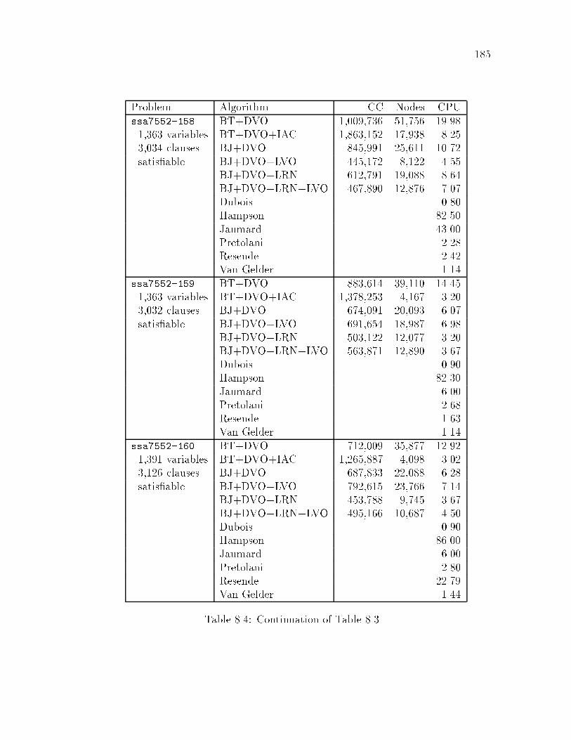
185

Problem Algorithm CC Nodes CPUssa7552-158 BT+DVO 1,009,736 51,756 19.981,363 variables BT+DVO+IAC 1,863,152 17,938 8.253,034 clauses BJ+DVO 845,991 25,611 10.72satis�able BJ+DVO+LVO 445,172 8,122 4.55

BJ+DVO+LRN 612,791 19,088 8.64BJ+DVO+LRN+LVO 467,890 12,876 7.07Dubois 0.80Hampson 82.50Jaumard 43.00Pretolani 2.28Resende 2.42Van Gelder 1.14

ssa7552-159 BT+DVO 883,614 39,110 14.451,363 variables BT+DVO+IAC 1,378,253 4,167 3.203,032 clauses BJ+DVO 674,091 20,093 6.07satis�able BJ+DVO+LVO 691,654 18,987 6.98

BJ+DVO+LRN 503,122 12,077 3.20BJ+DVO+LRN+LVO 563,871 12,890 3.67Dubois 0.90Hampson 82.30Jaumard 6.00Pretolani 2.68Resende 1.63Van Gelder 1.14

ssa7552-160 BT+DVO 712,009 35,877 12.921,391 variables BT+DVO+IAC 1,265,887 4,098 3.023,126 clauses BJ+DVO 687,833 22,088 6.28satis�able BJ+DVO+LVO 792,615 23,766 7.14

BJ+DVO+LRN 453,788 9,745 3.67BJ+DVO+LRN+LVO 495,166 10,687 4.50Dubois 0.90Hampson 86.00Jaumard 6.00Pretolani 2.80Resende 22.79Van Gelder 1.44

Table 8.4: Continuation of Table 8.3.

186

great savings in CPU time. This pattern was most pronounced on problems with

tight constraints. Look-ahead value ordering and jump-back learning both tended

to improve substantially the e�cacy of BJ+DVO. These enhancements too were

more e�ective on problems with tight constraints. Combining jump-back learning

and LVO into BJ+DVO+LRN+LVO did not tend to be particularly useful: in only

one experiment with random problems, based on parameters h300; 3; 0:0206; 0:222i,was this combination superior in CPU time to the other BJ+DVO variants. On the

other hand, BJ+DVO+LRN+LVO showed the best performance on the hardest

DIMACS Challenge problem, which suggests that the combination can be useful

on problems of su�cient size.

The e�ectiveness of interleaving arc-consistency was partly contingent on

the relatively low cost of performing a consistency check in our program. In the

experiment with parameters h200; 3; 0:0592; 0:111i, for instance, BT+DVO+IACperformed about 430,000 consistency checks per CPU second (23,836,368 / 55.44).

If consistency checking had been more expensive, the ranking of BT+DVO+IAC

relative to the other algorithms might have changed. Indeed, BT+DVO+IAC was

not quite such a strong performer on the DIMACS problems, which have a large

number on non-binary constraints. In our implementation, binary constraints were

stored in a table, which permits fast look-up, while higher order constraints were

stored in lists, to which access is slower.

8.6 Conclusions

We have shown that the trends observed in earlier chapters continue to hold

both for larger random problems and for a set of satis�ability problems drawn

from circuit analysis. Enforcing arc-consistency after each variable instantiation

improved the performance of BT+DVO by orders of magnitude on problems with

relatively tight constraints. Jump-back learning and look-ahead value ordering,

187

both individually and in combination, substantially improved the performance of

BJ+DVO.

Chapter 9

Encoding Maintenance

Scheduling Problems as CSPs

9.1 Overview of Chapter

This chapter focusses on a well-studied problem of the electric power in-

dustry: optimally scheduling preventative maintenance of power generating units

within a power plant. We de�ne a formal model which captures most of the in-

teresting characteristics of these problems, and then show how the model can be

cast as a constraint satisfaction problem. Because maintenance scheduling is an

optimization problem, we use a series of CSPs with ever-tightening constraints

to discover a locally optimal schedule. Empirical results show that applying the

learning algorithm from Chapter 7 signi�cantly reduces the CPU time required to

solve this series of maintenance scheduling CSPs.

9.2 Introduction

The problem of scheduling o�-line preventative maintenance of power gen-

erating units is of critical interest to the electric power industry. A typical power

plant consists of one or two dozen power generating units which can be individually

188

189

scheduled for maintenance. Both the required duration of each unit's preventa-

tive maintenance and a reasonably accurate estimate of the power demand that

the plant will be required to meet throughout the planning period are known in

advance. The general purpose of determining a maintenance schedule is to deter-

mine the duration and sequence of outages of power generating units over a given

time period, while minimizing operating and maintenance costs over the planning

period, subject to various constraints. A maintenance schedule is often prepared

in advance for a year at a time, and scheduling is done most frequently on a week-

by-week basis. The power industry generally considers shorter term scheduling,

up to a period of one or two weeks into the future, to be a separate problem called

\unit commitment."

Computational approaches to maintenance scheduling have been intensively

studied since the mid 1970's. Dopazo and Merrill [20] formulated the maintenance

scheduling problem as a 0-1 integer linear program. Zurm and Quintana [93] used a

dynamic programming approach. Egan [22] studied a branch and bound technique.

More recently, techniques such as simulated annealing, arti�cial neural networks,

genetic algorithms, and tabu search [45] have been applied.

This chapter reports the results of applying the constraint processing tech-

niques developed in the earlier chapters to the maintenance scheduling problem.

The task is of interest for several reasons. Primary, of course, is the opportu-

nity to take our research results \out of the lab," and to put them to use on

problems of substantial economic interest. Within the context of evaluating CSP

algorithms, applying the algorithms to maintenance scheduling-based problems

provides a testbed of problem instances that have an interesting structure and

non-binary constraints. Our preliminary empirical results indicate that algorithms

which are superior on random uniform binary CSPs are also superior on mainte-

nance scheduling problems, providing some validation of the empirical approach

in the earlier parts of this dissertation.

190

Week 1

Unit 1

Week 1

Unit 2

Week 1

Unit 3

Week 1

Unit 4

Week 1

Unit 5

Week 2

Unit 1

Week 2

Unit 2

Week 2

Unit 3

Week 2

Unit 4

Week 2

Unit 5

� � �

� � �

� � �

� � �

� � �

Wk 12

Unit 1

Wk 12

Unit 2

Wk 12

Unit 3

Wk 12

Unit 4

Wk 12

Unit 5

Figure 9.1: A diagrammatic representation of a maintenance scheduling constraintsatisfaction problem. Each circle stands for a variable representing the status ofone unit in one week. The dashed vertical ovals indicate constraints between allof the units in one week: meeting the minimum power demand and optimizingthe cost per week. The horizontal ovals represent constraints on one unit over theentire period: scheduling an adequate period for maintenance.

We also present a new use for learning. The constraint framework we use

consists entirely of so-called hard constraints, those which must be satis�ed for a

solution to be valid. Optimization problems sometimesmake use of soft constraints,

which can be partially satis�ed. To avoid introducing soft constraints, we approach

optimization as solving a series of related CSPs, each consisting solely of hard

constraints. The CSPs in the series di�er in that the constraint being optimized

is tighter in each succeeding problem in the series. The tighter constraints results

from a reduced cost bound in the function being optimized. Constraints learned

during one instance of the series can be applied again on later instances.

9.3 The Maintenance Scheduling Problem

As a problem for an electric power plant operator, maintenance scheduling

must take into consideration such complexities as local holidays, weather patterns,

191

constraints on suppliers and contractors, national and local laws and regulations,

and other factors that are germane only to a particular power plant. We have

developed a slightly simpli�ed model of the maintenance scheduling problem. Our

model is similar to those appearing in most scholarly articles, and follows closely

the approach of Yellen and his co-authors [2, 92]. The maintenance scheduling

problem can be represented by a rectangular matrix (see Fig. 9.1). Each entry in

the matrix represents the status of one generating unit for one week. (Since the

time minimum period considered is almost always the week, we will use the terms

week and time period interchangeably.) A unit can be in one of three states: on,

off, or maint.

9.3.1 Parameters

A speci�c maintenance scheduling problem, in our formulation, is de�ned

by a set of parameters, which are listed in Fig. 9.2. Parameters U , the number

of units, and W , the number of weeks, control the size of the schedule. Many

power plants have a �xed number of crews which are available to carry out the

maintenance; therefore the parameter M speci�es the maximum number of units

which can be undergoing maintenance at any one time.

In this paragraph and elsewhere in the chapter we adopt the convention

of quantifying the subscript i over the number of units, 1 � i � U , and the

subscript t over the number of weeks, 1 � t � W . Several parameters specify the

characteristics of the power generating units. The costs involved in preventative

maintenance, mit, can vary from unit to unit and from week to week; for instance,

hydroelectric units are cheaper to maintain during periods of low water ow. The

predicted operating cost of unit i in week t is given by cit. This quantity varies

by type of unit and also in response to fuel costs. For example, the fuel costs

of nuclear units are low and change little over the year, while oil-�red units are

typically more expensive to operate in the winter, when oil prices often increase.

192

Input:U number of power generating unitsW number of weeks to be scheduledM maximum number of units which can be maintained simultaneouslymit cost of maintaining unit i in period tcit operating cost of unit i in period tki power output capacity of unit iei earliest maintenance start time for unit ili latest maintenance start time for unit idi duration of maintenance for unit iN set of pairs of units which cannot be maintained simultaneouslyDt energy (output) demand in period t

Output:xit status of unit i in period t: on, off or maint

Figure 9.2: Parameters which de�ne a speci�c maintenance scheduling problem.

Parameter ki speci�es the maximum power output of unit i. Most formula-

tions of maintenance scheduling consider this quantity constant over time, although

in reality it can uctuate, particularly for hydro-electric units.

The permissible window for scheduling the maintenance of a unit is controlled

by parameters ei, the earliest starting time, and li, the latest allowed starting time.

These parameters are often not utilized (that is, ei is set to 1 and li is set to W )

because maintenance can be performed at any time. However, the maintenance

window can be used to prevent hydro-electric power plants from being maintained

during periods of high water ow, or for accommodating holiday and vacation

seasons. The duration of maintenance is speci�ed by parameter di.

Sometimes the maintenance of two particular units cannot be allowed to

overlap, since they both require a particular unique resource, perhaps a piece of

equipment or a highly trained crew member. Such incompatible pairs of units are

speci�ed in the set N = f(i1; i2); . . . ; (in�1; in)g.

The �nal input parameter, Dt, is the predicted power demand on the plant

in each week t.

193

The parameters xit are the output of the scheduling procedure, and de�ne

the maintenance schedule. xit can take on one of three values:

� on: unit i is on for week t, can deliver ki power for the week, and will cost

cit to run;

� off: unit i is o� for week t, will deliver no power and will not result in any

cost;

� maint: unit i is being maintained for week t, will deliver no power, and will

cost mit.

It is worth pointing out that generating units can often be operated at any level

of output between zero power and full power, with a corresponding decrease in

the cost of operating the unit. Some maintenance scheduling systems schedule

all non-maintained units as on, and assume that to meet the demand of each

period, units which are not on maintenance pick up power in ascending order of

fuel cost [45]. However, determining operating levels is usually not considered part

of maintenance scheduling, and a two- or three-value approach such as we have

adopted (e.g. on, off, maint) is more widely followed.

9.3.2 Constraints

A valid maintenance schedule must meet the following constraints or domain

requirements, which arise naturally from the de�nition and intent of the parame-

ters.

First, the schedule must permit the overall power demand of the plant to be

met for each week. Thus the sum of the power output capacity of all units not

scheduled for maintenance must be greater than the predicted demand, for each

week. Let zit = 1 if xit = on, and 0 otherwise. Then the schedule must satisfy the

following inequalities.

Xi

zitki � Dt for each time period t (9:1)

194

The second constraint is that maintenance must start and be completed

within the prescribed window, and the single maintenance period must be con-

tinuous, uninterrupted, and of the desired length. The following conditions must

hold true for each unit i.

(start) if t < ei then xit 6= maint (9.2)

(end) if t � li + di then xit 6= maint (9.3)

(continuous) if xit1 = maint and xit2 = maint and t1 < t2

then for all t; t1 < t < t2; xit = maint (9.4)

(length) if t1 = mint(xit = maint) and t2 = max

t(xit = maint)

then t2 � t1 + 1 = di (9.5)

(existence) 9t such that xit = maint (9.6)

The third constraint is that no more than M units can be scheduled for

maintenance simultaneously. Let yit = 1 if xit = maint, and 0 otherwise.

Xi

yit �M for each time period t (9:7)

The �nal constraint on a maintenance schedule is that incompatible pairs of units

cannot be scheduled for simultaneous maintenance.

if (i1; i2) 2 N and xi1t = maint then xi2t 6= maint for each time period t

(9:8)

After meeting the above constraints, we want to �nd a schedule which min-

imizes the maintenance and operating costs during the planning period. Let

wit = mit if xit = maint, cit if xit = on, and 0 if xit = off.

MinimizeXi

Xt

wit (9:9)

Objective functions other than (9.9) can also be used. For example, it may be

necessary to reschedule the projected maintenance midway through the planning

195

period. In this case, a new schedule which is as close as possible to the previous

schedule may be desired, even if such a schedule does not have a minimal cost.

We have now stated precisely the parameters, constraints and optimization

function that de�ne a maintenance scheduling problem.

9.4 FormalizingMaintenance Problems as CSPs

Given the de�nition of the maintenance scheduling problem presented in the

previous section, there exist several ways to encode the problem in the constraint

satisfaction framework. Formalizing a maintenance scheduling problem as a con-

straint satisfaction problem entails deciding on the variables, the domains, and

the constraints which will represent the requirements of the problem. The goal of

course is to develop a scheme that is conducive to �nding a solution { a schedule

{ speedily. A CSP in general will be easier to solve if it has a smaller number of

variables, a smaller number of values per variable, and constraints of smaller arity.

(The arity of a constraint is the number of variables it refers to.) Since these three

conditions cannot be met simultaneously, compromises must be made to achieve a

satisfactory representation as a constraint satisfaction problem.

Our system encodes maintenance scheduling problems as CSPs with 3�U�Wvariables. The variables can be divided into a set of U�W visible variables, and two

U �W size sets of hidden variables. Of course the distinction between visible and

hidden variables is used for explanatory purposes only; the CSP solving program

treats each variable in the same way. Each variable has two or three values in its

domain. Both binary and higher arity constraints appear in the problem.

We label the visible variables Xit; they correspond directly to the output

parameters xit of the problem de�nition. Because i ranges from 1 to U and t

ranges from 1 to W , there are U �W visible variables. Each Xit has the domain

fon, off, maintg, corresponding exactly to the values of xit.

196

The �rst set of hidden variables, Yit, signi�es the maintenance status of unit

i during week t. The domain of each Y variable is ffirst, subsequent, notg.Yit = first indicates that week t is the beginning of unit i's maintenance period.

Yit = subsequent indicates that unit i is scheduled for maintenance during week

t and for at least one prior week. If Yit = not, then maintenance for unit i is not

planned during week t. The following constraint between each Xit and Yit variable

is required to keep the two variables synchronized (we list the compatible value

combinations):

Xit Yit

on not

off not

maint first

maint subsequent

The second set of hidden variables, Zit, are boolean variables which indicate

whether unit i is producing power output during week t. The two values for each

Z variable are fnone, fullg, corresponding to no power output and full power

output. Binary constraints between each Xit and the corresponding Zit variable

are as follows, again listing the legal combinations:

Xit Zit

on full

off none

maint none

The hidden variables triple the size of the CSP. The reasons for creating them

will become clear as we now discuss how the constraints are implemented.

Constraint (9.1) { weekly power demand

Each demand constraint involves the U visible variables that relate to a

particular week. The basic idea is to enforce a U -ary constraint between these

variables which guarantees that enough of the variables will be on to meet the

197

power demand for the week. This constraint can be implemented as a table of either

compatible or incompatible combinations, or as a procedure which takes as input

the U variables and returns true or false. Our implementation uses a table of

incompatible combinations. For example, suppose there are four generating units,

with output capacities k1=100; k2=200; k3=300; k4=400. For week 5, the demand

D5=800. The following 4-ary constraint among variables (Z1;5; Z2;5; Z3;5; Z4;5) is

created (incompatible tuples are listed).

Z1;5 Z2;5 Z3;5 Z4;5 comment (output level)

none none none none 0

none none none full 400

none none full none 300

none none full full 700

none full none none 200

none full none full 600

none full full none 500

full none none none 100

full none none full 500

full none full none 400

full full none none 300

full full none full 700

full full full none 600

Because the domain size of the Z variables is 2, a U -ary constraint can have as

many as 2U �1 tuples. If this constraint were imposed on the X variables directly,

which have domains of size 3, there would be 79 tuples (34 � 5) instead of 13

(24� 3). This is one reason for creating the hidden Z variables: to reduce the size

of the demand constraint.

A relation such as that in the above table may be projected onto a subset

of its variables, by listing the combinations of values which are restricted to this

subset. The relation's projection onto (Z1;5; Z2;5), for example, is

198

Z1;5 Z2;5

none none

none full

full none

full full

Tuples in the new, projected relation which appear with all possible combinations

of the remaining variables in the original relation may be recorded as smaller

constraints. That is, the binary constraint over the pair (Z1;5; Z2;5), allowing (Z1;5=

none; Z2;5=none) while the remaining tuples are not allowed, is implied by the

4-ary constraint. It is clearly desirable to recognize these smaller constraints prior

to search, and our system does so. In e�ect, the system notices that if Z1;5 is none

and Z2;5 is none, then the demand constraint for week 5 cannot be met, whatever

the status of the other units.

Constraints (9.2) and (9.3) { earliest and latest maintenance start date

These constraints are easily implemented by removing the value first from

the domains of the appropriate Y variables. The removal of a domain value is

often referred to as imposing a unary constraint.

Constraint (9.4) { continuous maintenance period

To encode this domain constraint in our formalism, we note that if the fol-

lowing three conditions hold, then maintenance will be for a continuous period:

1. There is only one �rst week of maintenance.

2. Week 1 cannot be a subsequent week of maintenance.

3. Every subsequent week of maintenance must be preceded by a �rst week of

maintenance or a subsequent week of maintenance.

Each of these conditions can be enforced by unary or binary constraints on the

Y variables. To enforce condition 1, for every unit i and pair of weeks t1 and

199

t2; t1 6= t2, we add the following binary constraint to the CSP (disallowed tuple

listed):

Yit1 Yit2

first first

Condition 2 is enforced by a unary constraint removing subsequent from the

domain of each Yi1 variable. Condition 3 is enforced by the following constraint

for all t > 1 (disallowed tuple listed):

Yit�1 Yit

not subsequent

Constraint (9.5) { length of maintenance period

A maintenance period of the correct length cannot be too short or too long.

If unit i's maintenance length di=1, then too short is not possible (constraint (9.6)

prevents non-existent maintenance periods); otherwise, for each unit i, each time

period t, and every t1; t < t1 < t + di, the following binary constraint exists to

prevent a short maintenance period (disallowed tuple listed):

Yit Yit1

first not

To ensure that too many weeks of maintenance are not scheduled, it is only neces-

sary to prohibit a subsequent maintenance week in the �rst week that maintenance

should have ended. This results in the following constraint for each i and t, letting

t1 = t+ di (disallowed tuple listed):

Yit Yit1

first subsequent

Constraint (9.6) { existence of maintenance period

This requirement is enforced by a high arity constraint among the Y variables

for each unit. Only the weeks between the earlist start week and the latest start

200

week need be involved. At least one Yit; ei � t � li, must have the value start.

It is simpler to prevent them from all having the value not, and let constraints

(9.4) and (9.5) ensure that a proper maintenance period is established. Thus the

(li � ei + 1)-arity constraint for each unit i is (disallowed tuple listed):

Yili . . . Yiei

not not not

Constraint (9.7) { no more than M units maintained at once

If M units are scheduled for maintenance in a particular week, constraints

must prevent the scheduling of an additional unit for maintenance during that

week. Thus the CSP must have (M + 1)-ary constraints among the X variables

which prevent anyM+1 from having the value of maint in any given week. There

will be�

UM+1

�of these constraints for each of the W weeks. They will have the

form (disallowed tuple listed):

Xi1t . . . XiM t

maint maint maint

Constraint (9.8) { incompatible pairs of units

The requirement that certain units not be scheduled for overlapping mainte-

nance is easily encoded in binary constraints. For every week t, and for every pair

of units (i1; i2) 2 N , the following binary constraint is created (incompatible pair

listed):

Xi1t Yi2t

maint maint

Objective function (9.9) { minimize cost

To achieve optimization within the context of our constraint framework, we

create a constraint that speci�es the total cost must be less that or equal to a set

amount. In order to reduce the arity of the cost constraint, we optimize cost by

week instead of over the entire planning period. The system therefore achieves a

201

local optimum in that sense and not necessarily a global optimum. Further study

is need to assess the trade-o�s between constraint size and global optimality.

We implemented the cost constraint as a procedure in our CSP solving pro-

gram. This procedure is called after each X type variable is instantiated. The

input to the procedure is the week, t, of the variable, and the procedure returns

true if the total cost corresponding to week t variables assigned on or maint

is less than or equal to Ct, a new problem parameter (not referenced in Fig. 9.2)

which speci�es the maximum cost allowed in period t.

9.4.1 Solution Procedure

In order to achieve a locally optimal schedule, the Ct parameters are initially

set to high values, for which it is easy to �nd an acceptable maintenance schedule.

The Ct values are gradually lowered in unison, until a cost level is reached for which

no schedule exists. The previously discovered schedule is then reported. To make

this process more e�cient, we can incorporate jump-back learning, as described

in Chapter 7. After the problem with a certain level of Ct is solved successfully,

the new constraints recorded by learning are used in subsequent attempts to �nd

a schedule with lower Ct.

Two improvements to our procedure can be envisioned. Currently, we reduce

Ck and stop when no schedule can be found. A more e�cient approach is inspired

by binary search: set Ck to a high value H (for which a schedule is found quickly),

then to a low value L (for which the non-existence of a schedule is found quickly),

then to (H + L)=2 (for which a schedule may or may not be found), and so on,

according to the dictates of binary search. Implementing this strategy requires an

enhancement to our learning scheme, for after a round where no schedule is found

and Ck must be adjusted upwards, the new constraints recorded in the latest pass

must be removed from the database of constraints. Currently our system has

no way to distinguish constraints added by learning from those which existed at

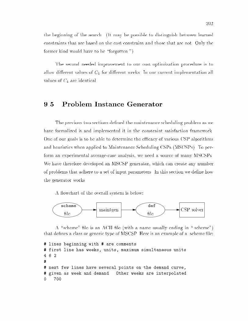
202

the beginning of the search. (It may be possible to distinguish between learned

constraints that are based on the cost constraint and those that are not. Only the

former kind would have to be \forgotten.")

The second needed improvement to our cost optimization procedure is to

allow di�erent values of Ck for di�erent weeks. In our current implementation all

values of Ck are identical.

9.5 Problem Instance Generator

The previous two sections de�ned the maintenance scheduling problem as we

have formalized it and implemented it in the constraint satisfaction framework.

One of our goals is to be able to determine the e�cacy of various CSP algorithms

and heuristics when applied to Maintenance Scheduling CSPs (MSCSPs). To per-

form an experimental average-case analysis, we need a source of many MSCSPs.

We have therefore developed an MSCSP generator, which can create any number

of problems that adhere to a set of input parameters. In this section we de�ne how

the generator works.

A owchart of the overall system is below:

.scheme

�lemaintgen

.def

�leCSP solver

A \scheme" �le is an ACII �le (with a name usually ending in \.scheme")that de�nes a class or generic type of MSCSP. Here is an example of a .scheme �le:

# lines beginning with # are comments

# first line has weeks, units, maximum simultaneous units

4 6 2

#

# next few lines have several points on the demand curve,

# given as week and demand. Other weeks are interpolated.

0 700

203

3 1000

# end this list with EOL

EOL

#

# next line has initial max cost per week, and decrement amount

60000 3000

#

# next line has average unit capacity and standard deviation

200 25

#

# next line has average unit maintenance time and std. dev.

2 1

#

# next line has standard deviation for maintenance costs

1000

#

# next few lines have some points on the maintenance cost curve,

# first number is week, then one column per unit

0 10000 10000 10000 10000 10000 10000

3 13000 16000 19000 10000 7000 10000

#

# next number is standard deviation for operating costs

2000

# next few lines have some points on the operating cost curve,

# first number is week, then one column per unit

0 5000 5000 5000 5000 5000 5000

# the next line specifies the number of incompatible pairs

2

# and that's it!

The maintgen program reads in a scheme �le and creates one or more speci�c

MSCSP instances in a .def �le which can be solved by the CSP solver. The maint-

gen program reads from the command line a random number generator seed and

a number indicating how many individual problems should be written to the .def

�le created as output. With one scheme �le and a seed, any number of MSCSPs

can be created; the same instances can easily be recreated later, provided that the

same seed is used.

204

5 10 15 20 24

500

800

1000

1500

��

� �

�� � �� �

� � �� � �

� �� �

� ����

� demand speci�ed in scheme �le� interpolated demand

Week

Demand

Figure 9.3: Weekly demand generated by the maintgen program when the following(week, demand) points are speci�ed: (5, 800), (10, 10,000), (18, 1,500), (20, 1,500),(24, 500).

The �rst line (ignoring comment lines which begin with \#") of the scheme

�le speci�es the fundamental size parameters of the MSCSPs which will be gener-

ated: the number of weeks W , the number of generating units U , and the number

of units which can be maintained at one timeM .

The scheme �le speci�es the demand for any number of weeks. The demand

for weeks that are not explicitly speci�ed is computed by a linear interpolation

between the surrounding speci�ed weeks. The process is shown diagrammatically

in Fig. 9.3. There is no randomness in the demand \curve" that is created based

on a scheme �le. Note that the weeks are numbered starting from 0, so that in

this example the last of the 25 weeks is week #24.

The following line in the scheme �le speci�es the initial maximum cost per

week, and the amount it is to be decremented after each successful search for a

schedule.

The characteristics of the units, that is, their output capacities and required

maintenance times, are not speci�ed individually in the scheme �le. Instead, these

values are randomly selected from normal distributions that have the means and

205

standard deviations speci�ed on the following two lines. Currently the earliest and

latest maintenance start dates are not speci�ed in the scheme �le, and are always

set to 0 and W � 1 in the .def �le.

Maintenance costs are speci�ed in the following lines of the scheme �le by

entering �rst the standard deviation (1,000 in the example), and then a table which

has a \week" column and then one column per unit. As with demand, values for

weeks that are not entered are interpolated. However, for maintenance costs there

is a random element; the interpolated value is used as the mean, together with the

speci�ed standard deviation. Operating costs are de�ned in the lines following the

maintenance costs, with exactly the same structure.

The last piece of information is the number of incompatible pairs of units.

The requested number of pairs is created randomly from a uniform distribution of

the units.

Here is an example of the .def �le created using the scheme �le above and

the random number seed 12345:

# comments begin with #

# first line has weeks W, units U, max-simultaneous M

4 6 2

# demand, one line per week

700

800

900

1000

# next few lines has maximum cost per week.

# Cost must be <= max.

60000 3000

# one line per unit:

# capacity maint length earliest maint start latest maint start

194 1 0 3

171 3 0 3

209 1 0 3

166 1 0 3

219 2 0 3

217 2 0 3

206

# maintenance costs, one line per week, one column per unit

11085 10034 9374 8945 10858 10045

11056 11988 13670 10465 9301 10625

12745 14625 15422 10422 8099 7629

12534 15394 21098 9841 6748 9364

# operating costs, one line per week, one column per unit

4284 6857 3847 5050 5145 4998

5987 7352 1967 4635 6152 4635

3746 6475 5151 3988 8172 4131

6152 3436 5475 5600 4366 6070

# incompatible pairs of units (numbering starts from 0)

1 3

2 3

EOL

# and that's it!

The def �le is in a format which is recognized by our CSP solver. The data

in the �le follows directly from the scheme �le, and corresponds to the parameters

in Fig. 9.2. The �rst line de�nes parameters W , U , and M . Next are W lines with

demand informations, Dt. The following line holds the maximum cost Ct (they

are all set to the same value) and the amount by which Ct is decremented.

The subsequent lines of the def �le specify, for each unit, the parameters ki,

di, ei, and li. Following them is a maintenance cost table with one value for each

mit and an operating cost table with one value for each cit. The incompatible pairs

of units from which the N set is constructed are listed, one pair per line. \EOL"

marks the end of this list.

207

# test4.scheme

# W, U, M

13 15 3

#

# Some weeks on the demand curve.

0 10000

12 13000

EOL

# Initial max cost per week, and decrement amount

110000 5000

#

# Average unit capacity and standard deviation

1000 100

#

# Average unit maintenance time and std. dev.

2 1

#

# Standard deviation for maintenance costs

1000

#

# Some points on the maintenance cost curve,

0 10000 10000 10000 10000 10000 10000 10000 10000 \

10000 10000 10000 10000 10000 10000 10000

12 10000 10000 10000 10000 10000 10000 10000 10000 \

10000 12000 12000 12000 12000 12000 12000

#

# Standard deviation for operating costs

1000

# Operating costs

0 5000 6000 4000 5000 6000 4000 5000 6000 \

4000 5000 4000 6000 5000 5000 8000

# the next line specifies the number of incompatible pairs

5

Figure 9.4: The scheme �le used to generate MSCSPs.

208

9.6 Experimental Results

To demonstrate the e�ectiveness of the constraint processing framework, we

present the results of experiments with two sets of MSCSPs. Experiments were

based on 100 random MSCSP generated according to the parameters in the scheme

�le listed in Fig. 9.4, and 100 larger random instances based on a similar scheme

�le. The smaller problems had 15 units and 13 time periods, creating 585 variables.

The larger problems had 20 units and 20 time periods, creating 1200 variables.

9.6.1 Optimization with learning

In the �rst experiment, we tried to �nd an optimal schedule for each MSCSP

in the smaller and larger sets. We used the iterative cost-bound procedure de-

scribed above. The results are shown in Fig. 9.5 and Fig. 9.6. BJ+DVO was the

base algorithm, with jump-back learning as described in Chapter 7. The learning

order was set to six; new constraints above that size were not recorded. We also

found schedules using BJ+DVO without learning.

Among the 100 smaller problems, all 100 MSCSPs had schedules at cost

bound 85,000 and above. Only 38 had schedules within the 80,000 bound; at 75,000

only four problems were solvable. On the set of 100 larger MSCSPs, schedules

were found for all instances at cost bound 120,000 and above. 97 instances had

schedules at cost bound 115,000 and 110,000; 11 at cost bound 105,000; and two

at cost bound 100,000 and 95,000.

The use of learning improved the performance of the BJ+DVO algorithm

on these random maintenance scheduling problems. For instance, on the smaller

problems, after �nding a schedule with cost bound 95,000, the average number of

learned constraints was 214. Tightening the cost bound to 90,000 resulted in over

twice as muchCPU timeneeded for BJ+DVOwithout learning (54.01 CPU seconds

compared to 23.28), but only a 71% increase for BJ+DVO with learning (29.41

209

� with learning? without learning� cum. constraints

110 105 100 95 90 85 80 75

cost bound (in thousands)

10

20

30

40

50

60

70

80

90

CPU

� � �

�

� �

�

�

? ? ?

?

?

?

?

?

100

200

300

400

� �

�

�

�

� � �

Figure 9.5: Average CPU seconds on 100 small problems (15 units, 13 weeks)to �nd a schedule meeting the cost bound on the y-axis, using BJ+DVO withlearning (�) and without learning (?). Cumulative number of constraints learnedcorresponds to right-hand scale.

compared to 17.20). Learning was less e�ective on the larger MSCSPs. Although

using learning reduced average CPU time, the improvement over BJ+DVOwithout

learning was much less than on the smaller problems.

9.6.2 Comparison of algorithms

The second experiment utilized the same sets of 100 smallerMSCSP instances

and 100 larger instances, but we did not try to �nd an optimal schedule. For the

smaller problems we set the cost bound at 85,000 and for the larger problems we

set the cost bound at 120,000. Each bound was the lowest level at which schedules

could be found for all problems. We used �ve of the six algorithms compared in

Chapter 8 to �nd a schedule for each problem. BT+DVO was omitted because in

210

� with learning? without learning� cum. constraints

150 145 140 135 130 125 120 115 110 105 100 95

cost bound (in thousands)

100

200

300

400

500

600

700

800

900

1000

CPU

� � ��

�� �

��

� � �

? ? ??

?

??

?

?

? ??

100

200

300

400

500

� �

��

�

� � � � � � �

Figure 9.6: Average CPU seconds on 100 large problems (20 units, 20 weeks)to �nd a schedule meeting the cost bound on the y-axis, using BJ+DVO withlearning (�) and without learning (?). Cumulative number of constraints learnedcorresponds to right-hand scale.

preliminary experiments it required several CPU hours per small problem, com-

pared to approximately a minute per problem for the other algorithms. The results

are summarized in Table 9.1.

Among the �ve algorithms, BJ+DVO performed least well on the smaller

problems and best on the larger problems, when average CPU time is the crite-

rion. BT+DVO+IAC was the best performer on the smaller problems and the

worst on the larger problems. This reversal in e�ectiveness may be related to the

increased size of the higher arity constraints on the larger problems. The high

arity constraints, such as those pertaining to the cost bound, the weekly power

demand, and the existence of a maintenance period, become looser as the number

of units and number of weeks increase. Results from earlier chapters indicated that

more look-ahead was e�ective on problems with tight constraints, and detrimental

on problems with loose constraints. Although as similar pattern was observed in

211

AverageAlgorithm CC Nodes CPU100 smaller problems:BT+DVO+IAC 315,988 3,761 51.65BJ+DVO 619,122 8,981 70.07BJ+DVO+LVO 384,263 5,219 54.48BJ+DVO+LRN 671,756 8,078 67.51BJ+DVO+LRN+LVO 476,901 5,085 57.45100 larger problems:BT+DVO+IAC 7,673,173 32,105 694.02BJ+DVO 2,619,766 28,540 460.42BJ+DVO+LVO 6,987,091 26,650 469.65BJ+DVO+LRN 5,892,065 27,342 521.89BJ+DVO+LRN+LVO 6,811,663 26,402 475.12

Table 9.1: Statistics for �ve algorithms applied to MSCSPs.

Chapter 4 for backjumping, nevertheless backjumping remains an e�ective tech-

nique on the larger problems. Further experiments are required to determine how

the relative e�cacy of di�erent algorithms is in uenced by factors such as the

size of the problem (number of weeks and units) and characteristics such as the

homogeneity of the units.

As we have done in earlier chapters, we also summarize our experiments by

estimating the parameters of the Weibull distribution. Fig. 9.7 shows plots of

Weibull distributions curves, based on data from the experiment with 100 large

scheduling problems. Data on consistency checks is represented in the top chart

of Fig. 9.7, and data on CPU time in the bottom chart. The procedure, as in

earlier chapters, was to estimate the parameters of the Weibull distribution using

techniques described in Chapter 3. Each curve on the charts in Fig. 9.7 shows

the estimated Weibull distribution for one algorithm. The estimated � values are

between 0.39 and 0.61. This range is similar to what we observed on experiments

with random binary problems. These small values of � denote a large variance

in the results, with many problem instances being relatively easy and a few much

harder.

212

large maintance scheduling problemsBT+DVO+IAC: �=4:42e-7 �=0:39 �=587,912BJ+DVO: �=1:13e-6 �=0:42 �=51,711BJ+DVO+LVO: �=2:71e-7 �=0:51 �=78,514BJ+DVO+LRN: �=2:64e-7 �=0:58 �=41,985BJ+DVO+LRN+LVO: �=2:11e-7 �=0:62

�=37,644

0 1,000,000 4,000,000 7,000,000Consistency Checks

Frequency

.05

.10

.15

.20

IAC

BJ+DVO

large maintance scheduling problemsBT+DVO+IAC: �=0:0536 �=0:43 �=45.8BJ+DVO: �=0:00627 �=0:42 �=3.7BJ+DVO+LVO: �=0:00420 �=0:50 �=3.6BJ+DVO+LRN: �=0:00294 �=0:59 �=3.5BJ+DVO+LRN+LVO: �=0:00311 �=0:61

�=3.5

0 50 200 350CPU seconds

Frequency

.05

.10

.15

.20

IAC

Figure 9.7: Weibull curves based on solvable \large" maintenance scheduling prob-lems generated with whatever. The top chart is based on consistency checks, thebottom chart on CPU seconds. �, �, and � parameters were estimated using theModi�ed Moment Estimator (see Chapter 3). The LVO, LRN, and LRN+LVOcurves on the top chart are almost indistinguishable, as are all distributions exceptthe one for BT+DVO+IAC in the bottom chart.

213

9.7 Conclusions

The constraint satisfaction problems derived from the maintenance schedul-

ing needs of the electric power industry are an interesting testbed for the CSP

algorithms developed in the earlier chapters. The problems have a mixture of

tight binary constraints, such as those that bind the X and Y variables together,

and loose high arity constraints, such as those that ensure that at least one main-

tenance period is scheduled for each unit. Perhaps the most promising algorithm

for these problems is learning, which seems from preliminary evidence to be a

useful part of performing optimization in the CSP framework. Further studies on

larger maintenance scheduling CSPs is required to determine whether one algo-

rithm dominates the others as problem size increases.

A challenging problem that is di�cult to formalize is to �nd the best way

to encode the requirements of a problem such as maintenance scheduling into

constraints of a CSP. In section 9.4 we discussed some of the trade-o�s involved

in, for example, adding \hidden" variables in return for a smaller number of tuples

in high arity constraints. This is a challenging area for future research that has

the potential of greatly impacting the applicability of the constraint satisfaction

framework to problems from science and industry.

Chapter 10

Conclusions

10.1 Contributions

The hypothesis underlying this research is that backtracking based search al-

gorithms that incorporate sophisticated \look-ahead" techniques that query, prune,

evaluate, and rearrange the future search space can be particularly e�ective algo-

rithms for constraint satisfaction problems. One premise we have relied on and

seen borne out multiple times is that most techniques for solving constraint sat-

isfaction problems are not competitors, but potential allies. On su�ciently large

and di�cult problems, multiple arrows in the quiver will not be redundant.

The algorithms presented in the work are new combinations of previously

existing, well-proven techniques. The BJ+DVO algorithm is based on Prosser's

con ict-directed backjumping [68], which is itself a \marriage," as Prosser calls it,

of Gaschnig's backjumping [31] and Dechter's graph-based backjumping [15]. The

look-ahead technique and dynamic variable ordering heuristic in BJ+DVO are due

to Haralick and Elliott [40], but both ideas appear earlier in the literature. Our

experiments showed that the components of BJ+DVO work together in a way that

is more e�ective than any of the constituent parts individually.

Look-ahead value ordering processes the variables which have not yet been

assigned values in order to choose a value for the current variable. This idea �rst

appeared in Dechter [19], using a di�erent scheme to examine the future variables.

214

215

LVO uses the same look-ahead e�ort already employed by BJ+DVO, allowing

the combination BJ+DVO+LVO to bene�t twice from its processing of future

variables. The LVO heuristic proved in our experiments to be especially helpful

on the hardest constraint satisfaction problems.

The new learning algorithm we presented, jump-back learning, takes advan-

tage of the con ict set already maintained by backjumping for search control. This

technique makes the additional cost of recording constraints at dead-ends almost

negligible. Whether the costs of accessing the learned constraints is more or less

than the bene�t they provide by pruning the search space was investigated em-

pirically. Our experiments showed that when the order of learning (the maximum

size of a new constraint) was limited, the bene�ts of learning usually outweighed

the costs. We showed that learning can also play an important role in solving

optimization problems in the CSP framework. In the context of maintenance

scheduling problems for the electric power industry, optimization was presented

as solving a series of CSP decision problems, with cost bound constraints being

iteratively adjusted until an optimum is reached. Our experiments idicated that

if constraints learned in one iteration are applied again in subsequent attempts to

solve the problem, a substantial bene�t is realized.

In addition to proposing new combination algorithms, the dissertation pro-

vides extensive empirical evaluation of them. Algorithms were run and compared

on three types of problems: random binary CSPs, circuit problems encoded as

CSPs, and maintenance scheduling problems encoded as CSPs. A distinguishing

feature of the research presented in this dissertation is that experiments were per-

formed on larger and harder random CSP instances than have previously been

reported. Our empirical results indicated that each of the new algorithm combi-

nations became increasingly more e�ective as problems became larger and harder.

This is good news, because scheduling, planning, optimization, and con�guration

problems of interest to science and industry are often quite large. Combining

multiple techniques will no doubt be necessary to attack these problems as CSPs.

216

We proposed in Chapter 3 that when backtracking-based algorithms are ap-

plied to random binary CSPs, the distribution of sizes of the resulting search trees

can be closely approximated by standard continuous probability distributions. It

is necessary to segregate solvable and unsolvable problem instances. After doing

so, the empirical distribution of unsolvable problems is close to a lognormal dis-

tribution, and the empirical distribution of solvable problems is close to a Weibull

distributions. We used these distribution functions, along with estimated param-

eters, to report the results of several experiments in the dissertation.

10.2 Future Work

There are many directions in which this research can be extended. One

promising technique for combining multiple algorithms or heuristics is not to inte-

grate them into a single executable unit, but to run several algorithms in tandem,

either on parallel computers, or via time-slicing on a single CPU. All algorithms

then stop when a single algorithm returns an answer. The potential bene�t of this

scheme stems from the great variance in the time required to solve instances. This

variance has been observed not only over multiple instances drawn from a distribu-

tion of problems (as was the focus of Chapter 3), but also over multiple applications

of a single algorithm to a single instance, when points of non-determinacy in the

algorithm (for instance, variable and value ordering) are decided randomly [77]. It

may be possible to extend the analysis of distributions started in Chapter 3 to pro-

vide guidance in how much time should be allocated to each time-sliced algorithm.

In Chapter 3 the \completion rate" of an algorithm was de�ned as equivalent to

the well-known concept of the hazard rate in reliability theory. It is a measure

of the probability of completing the search in the next time unit. Knowledge of

the completion rate function can be used in resource-limited situations to suggest

an optimum time-bound for an algorithm to process a single instance. Examples

217

would be running multiple algorithms on a single instance in a time-sliced man-

ner, as proposed in [42], and environments where the goal is to complete as many

problems as possible in a �xed time period.

An exciting trend in CSP algorithms that has received intense interest re-

cently is the use of randomized or \local search" algorithms. These algorithms

essentially guess a solution, and if the guess proves wrong (as of course it almost

always does, initially) they are able to follow a gradient in the search space which,

it is hoped, leads towards a solution. A critical feature of these algorithms is that

if no solution is found after a certain bound on CPU time or subroutine calls,

the process is restarted with a new random guess. Several ways to combine ran-

domized search with techniques developed for backtracking have been proposed.

Because randomized approaches almost always involve multiple restarts on the

same instance, incorporating learning in random algorithms seems particularly

promising. For instance, if a new constraint is learned before each restart, then

as with backtracking-based search algorithms, the randomized algorithm will be

prevented from making the same mistake again.

A third interesting direction for further research is continued study of the

correlation between empirical distributions of e�ort and standard probability dis-

tributions from statistics. Perhaps the starting point should be to put the specula-

tions in the last section of Chapter 3 on a more rigorous footing. An explanation of

why the lognormal and Weibull distributions approximate the empirical distribu-

tions, based on both the mathematical derivation of the distribution functions, and

on the known properties of the CSP algorithms and the random problem distribu-

tions, might provide a deeper understanding of the search process, might lead to

improved algorithms, and might aid in the reporting of experiments with random

problems.

Our experiments with backjumping and look-ahead all relied on an amount

of look-ahead identical to that of forward checking. However, in Chapter 5 we

observed that for some types of problems a stronger amount of look-ahead, such

218

as arc-consistency, was bene�cial. We left open the interesting question of whether

there exist problem classes for which the combination of backjumping and inte-

grated arc-consistency is e�ective.

10.3 Final Conclusions

The goal of this dissertation has been to de�ne and evaluate algorithms that

combine several e�ective techniques. Most of the evaluation has been based on

random binary constraint satisfaction problems, an approach that has been used

in the �eld for over twenty years. Our interest in accurately summarizing the

results of large-scale experiments led to the study of the distribution of problem

di�culty. Because many real world problem have distinct structure and non-binary

constraints, we also used problems from DIMACS and the electric power industry

as a testbed for the algorithms. The conclusion we draw from all the experiments

is that no one algorithm is best for all problems, but that by combining several

techniques into one algorithm, and by selecting the right algorithm based on the

characteristics of the problem instance, a substantial increase in performance can

be achieved.

Bibliography

[1] J. Aitchison and J. A. C. Brown. The Lognormal Distribution. Cambridge

University Press, Cambridge, England, 1960.

[2] T. M. Al-Khamis, S. Vemuri, L. Lemonidis, and J. Yellen. Unit maintenance

scheduling with fuel constraints. IEEE Trans. on Power Systems, 7(2):933{

939, 1992.

[3] Fahiem Bacchus and Paul van Run. Dynamic Variable Ordering In CSPs.

In Ugo Montanari and Francesca Rossi, editors, Principles and Practice of

Constraint Programming, pages 258{275, 1995.

[4] Andrew B. Baker. Intelligent Backtracking on Constraint Satisfaction

Problems: Experimental and Theoretical Results. PhD thesis, University of

Oregon, Eugene, OR 97403, 1995.

[5] Roberto Bayardo and Daniel Mirankar. A complexity analysis of space-

bounded learning algorithms for the constraint satisfaction problem. In

Proceedings of the Thirteenth National Conference on Arti�cial Intelligence,

pages 298{304, 1996.

[6] Christian Bessi�ere. Arc-consistency and arc-consistency again. Arti�cial

Intelligence, 65:179{190, 1994.

[7] Christian Bessi�ere and Jean-Charles R�egin. MAC and Combined Heuristics:

Two Reasons to Forsake FC (and CBJ?) on Hard Problems. In Eugene C.

Freuder, editor, Principles and Practice of Constraint Programming { CP96,

pages 61{75, 1996.

[8] James R. Bitner and Edward M. Reingold. Backtrack Programming

Techniques. Communications of the ACM, 18(11):651{656, 1975.

219

220

[9] M. Bruynooghe and L. M. Pereira. Deduction revision by intelligent back-

tracking. In J. A. Campbell, editor, Implementation of Prolog, pages 194{215.

Ellis Horwood, 1984.

[10] Peter Cheeseman, Bob Kanefsky, and William M. Taylor. Where the really

hard problems are. In Proceedings of the International Joint Conference on

Arti�cial Intelligence, pages 331{337, 1991.

[11] A. C. Cohen and B. J. Whitten. Parameter Estimation in Reliability and Life

Span Models. Marcel Dekker, Inc., New York, 1988.

[12] J. M. Crawford and L. D. Auton. Experimental results on the crossover point

in satis�ability problems. In Proceedings of the Eleventh National Conference

on Arti�cial Intelligence, pages 21{27, 1993.

[13] M. Davis, G. Logemann, and D. Loveland. A Machine Program for Theorem

Proving. Communications of the ACM, 5:394{397, 1962.

[14] Martin Davis and Hilary Putnam. A Computing Procedure for Quanti�cation

Theory. Journal of the ACM, 7(3):201{215, 1960.

[15] Rina Dechter. Enhancement Schemes for Constraint Processing:

Backjumping, Learning, and Cutset Decomposition. Arti�cial Intelligence,

41:273{312, 1990.

[16] Rina Dechter. Constraint networks. In Encyclopedia of Arti�cial Intelligence,

pages 276{285. John Wiley & Sons, 2nd edition, 1992.

[17] Rina Dechter and Itay Meiri. Experimental evaluation of preprocessing algo-

rithms for constraint satisfaction problems. Arti�cial Intelligence, 68:211{241,

1994.

[18] Rina Dechter and Judea Pearl. Network-based heuristics for constraint-

satisfaction problems. Arti�cial Intelligence, 34:1{38, 1987.

[19] Rina Dechter and Judea Pearl. Tree-clustering schemes for constraint pro-

cessing. Arti�cial Intelligence, 38:353{366, 1989.

221

[20] J. F. Dopazo and H. M. Merrill. Optimal Generator Maintenance Scheduling

using Integer Programming. IEEE Trans. on Power Apparatus and Systems,

PAS-94(5):1537{1545, 1975.

[21] O. Dubois, P. Andre, Y. Boufkhad, and J. Carlier. SAT versus UNSAT.

In David S. Johnson and Michael A. Trick, editors, Cliques, Coloring, and

Sati�ability, volume 26 of DIMACS Series in Discrete Mathematics and

Theoretical Computer Science. American Mathematical Society, 1996.

[22] G. T. Egan. An Experimental Method of Determination of Optimal

Maintenance Schedules in Power Systems Using the Branch-and-Bound

Technique. IEEE Trans. SMC, SMC-6(8), 1976.

[23] Hani El Sakkout, Mark G. Wallace, and E. Barry Richards. An Instance of

Adaptive Constraint Propagation. In Eugene C. Freuder, editor, Principles

and Practice of Constraint Programming { CP96, pages 164{178, 1996.

[24] R. E. Fikes and N. J. Nilsson. A new approach to the application of theorem

proving to problem solving. Arti�cial Intelligence, 2:189{208, 1971.

[25] E. C. Freuder. A su�cient condition for backtrack-free search. JACM,

21(11):958{965, 1982.

[26] Daniel Frost and Rina Dechter. Dead-end driven learning. In Proceedings

of the Twelfth National Conference on Arti�cial Intelligence, pages 294{300,

1994.

[27] Daniel Frost and Rina Dechter. In search of the best constraint satisfac-

tion search. In Proceedings of the Twelfth National Conference on Arti�cial

Intelligence, pages 301{306, 1994.

[28] Daniel Frost and Rina Dechter. Look-ahead value ordering for constraint

satisfaction problems. In Proceedings of the Fourteenth International Joint

Conference on Arti�cial Intelligence, pages 572{578, 1995.

[29] Daniel Frost, Irina Rish, and Llu��s Vila. Summarizing csp hardness with con-

tinuous probability distributions. In Proceedings of the Sixteenth International

Joint Conference on Arti�cial Intelligence, pages 327{333, 1997.

222

[30] John G. Gaschnig. A General Backtrack Algorithm That Eliminates Most

Redundant Tests. In Proceedings of the International Joint Conference on

Arti�cial Intelligence, page 247, 1977.

[31] John G. Gaschnig. Performance Measurement and Analysis of Certain Search

Algorithms. PhD thesis, Carnegie Mellon University, Pittsburgh, PA 15213,

May 1979.

[32] Peter Andreas Geelen. Dual Viewpoint Heuristics for Binary Constraint

Satisfaction Problems. In 10th European Conference on Arti�cial Intelligence,

pages 31{35, 1992.

[33] Richard G�enisson and Phillippe J�egou. Davis and Putnam were already check-

ing forward. In 12th European Conference on Arti�cial Intelligence, pages

180{184, 1996.

[34] Ian P. Gent, Ewan MacIntyre, Patrick Prosser, Barbara M. Smith, and Toby

Walsh. An Empirical Study of Dynamic Variable Ordering Heuristics for the

Constraint Satisfaction Problem. In Eugene C. Freuder, editor, Principles and

Practice of Constraint Programming { CP96, pages 179{193, 1996.

[35] Ian P. Gent and Patrick Prosser. The 50% Point in Constraint-Satisfaction

Problems. Technical Report 95/180, Department of Computer Science,

University of Strathclyde, 1995.

[36] Matthew L. Ginsberg. Dynamic backtracking. Journal of Arti�cial

Intelligence Research, 1:25{46, 1993.

[37] Solomon W. Golomb and Leonard D. Baumert. Backtrack Programming.

Communications of the ACM, 12(4):516{524, 1965.

[38] Carla Gomes, Bart Selman, and Nuno Crato. Heavy-Tailed Distributions in

Combinatorial Search. In Gert Smolka, editor, Principles and Practice of

Constraint Programming { CP97, pages 121{135, 1997.

[39] Steven Hampson and Denis Kibler. Large Plateaus and Plateau Search

in Boolean Satis�ability Problems: When to Give Up Searching and Start

223

Again. In David S. Johnson and Michael A. Trick, editors, Cliques, Coloring,

and Sati�ability, volume 26 of DIMACS Series in Discrete Mathematics and

Theoretical Computer Science. American Mathematical Society, 1996.

[40] R. M. Haralick and G. L. Elliott. Increasing Tree Search E�ciency for

Constraint Satisfaction Problems. Arti�cial Intelligence, 14:263{313, 1980.

[41] Tad Hogg and Colin P. Williams. The hardest constraint satisfaction prob-

lems: a double phase transition (Research Note). Arti�cial Intelligence,

69:359{377, 1994.

[42] Bernardo A. Huberman, Rajan M. Lukose, and Tad Hogg. An Economics

Approach to Hard Computational Problems. Science, 275:51{54, 1997.

[43] Brigette Jaumard, Mihnea Stan, and Jacques Desrosiers. Tabu Search and a

Quadratic Relaxation for the Satis�ability Problems. In David S. Johnson and

Michael A. Trick, editors, Cliques, Coloring, and Sati�ability, volume 26 of

DIMACS Series in Discrete Mathematics and Theoretical Computer Science.

American Mathematical Society, 1996.

[44] David S. Johnson and Michael A. Trick, editors. Cliques, Coloring, and

Sati�ability, volume 26 of DIMACS Series in Discrete Mathematics and

Theoretical Computer Science. American Mathematical Society, Providence,

Rhode Island, 1996.

[45] Hyunchul Kin, Yasuhiro Hayashi, and Koichi Nara. An Algorithm for Thermal

Unit Maintenance Scheduling Through Combined Use of GA SA and TS.

IEEE Trans. on Power Systems, 12(1):329{335, 1996.

[46] Donald E. Knuth. Estimating the E�ciency of Backtrack Programs.

Mathmatics of Computation, 29(129):121{136, 1975.

[47] Grzegorz Kondrak and Peter van Beek. A Theoretical Evaluation of Selected

Backtracking Algorithms. Arti�cial Intelligence, 89:365{387, 1997.

[48] R. E. Korf. A program than learns how to solve Rubik's cube. In Proceedings

of the National Conference on Arti�cial Intelligence, pages 164{167, 1982.

224

[49] Alvin C. M. Kwan. Validity of Normality Assumption in CSP Research. In

PRICAI'96: Topics in Arti�cial Intelligence. Proc. of the 4th Paci�c Rim

International Conference on Arti�cial Intelligence, pages 253{263, 1996.

[50] A. K. Mackworth. Consistency in networks of relations. Arti�cial Intelligence,

8:99{118, 1977.

[51] A. K. Mackworth and E. C. Freuder. The complexity of some polynomial

network consistency algorithms for constraint satisfaction problems. Arti�cial

Intelligence, 25:65{74, 1985.

[52] Alan K. Mackworth. The logic of constraint satisfaction. Arti�cial

Intelligence, 58:3{20, 1992.

[53] Nancy R. Mann, Ray E. Schafer, and Nozer D. Singpurwalla. Methods for

Statistical Analysis of Reliability and Life Data. John Wiley and Sons, New

York, 1974.

[54] Steven Minton. Learning Search Control Knowledge: An Explanation-based

Approach. Kluwer Academic Publishers, 1988.

[55] Steven Minton. Qualitative Results Concerning the Utility of Explanation-

Based Learning. Arti�cial Intelligence, 42:363{392, 1990.

[56] Steven Minton, Mark D. Johnson, Andrew B. Phillips, and Philip Laird.

Solving Large-Scale Constraint Satisfaction and Scheduling Problems Using a

Heuristic Repair Method. In Proceedings of the Eighth National Conference

on Arti�cial Intelligence, pages 17{24, 1990.

[57] David Mitchell. Respecting Your Data (I). In AAAI-94 Workshop on

Experimental Evaluation of Reasoning and Search Methods, pages 28{31, 1994.

[58] David Mitchell, Bart Selman, and Hector Levesque. Hard and Easy

Distributions of SAT Problems. In Proceedings of the Tenth National

Conference on Arti�cial Intelligence, pages 459{465, 1992.

[59] R. Mohr and T. Henderson. Arc and path consistency revisited. Arti�cial

Intelligence, 25:65{74, 1986.

225

[60] U. Montanari. Networks of constraints: Fundamental properties and applica-

tions to picture processing. Inf. Sci., 7:95{132, 1974.

[61] Bernard A. Nadel. Tree search and arc consistency in constraint satisfac-

tion algorithms. In L. Kanal and V. Kumar, editors, Search in Arti�cial

Intelligence, pages 287{342. Springer, 1988.

[62] Bernard A. Nadel. Constraint satisfaction algorithms. Computational

Intelligence, 5:188{224, 1989.

[63] Bernard A. Nadel. Some applications of the constraint satisfaction problem.

Technical report, Wayne State University, 1990.

[64] Wayne Nelson. Accelerated Testing: Statistical Models, Test Plans, and Data

Analyses. John Wiley & Sons, New York, 1990.

[65] Bernard Nudel. Consistent-Labeling Problems and their Algorithms:

Expected-Complexities and Theory-Based Heuristics. Arti�cial Intelligence,

21:135{178, 1983.

[66] Judea Pearl. Heuristics. Addison-Wesley, Reading, Mass., 1985.

[67] Daniele Pretolani. E�ciency and Stability of Hypergraph SAT Algorithms.

In David S. Johnson and Michael A. Trick, editors, Cliques, Coloring, and

Sati�ability, volume 26 of DIMACS Series in Discrete Mathematics and

Theoretical Computer Science. American Mathematical Society, 1996.

[68] Patrick Prosser. Hybrid Algorithms for the Constraint Satisfaction Problem.

Computational Intelligence, 9(3):268{299, 1993.

[69] Patrick Prosser. Binary Constraint Satisfaction Problems: Some are Harder

than Others. In Proceedings of the 11th European Conference on Arti�cial

Intelligence (ECAI 94), pages 95{99, 1994.

[70] Patrick Prosser. Mac-cbj: maintaining arc consistency with con ict-directed

backjumping. Technical Report 95/177, The University of Strathclyde,

Glasgow, Scotland, Dept. of Computer Science, 1995.

226

[71] Paul Walton Purdom. Search Rearrangement Backtracking and Polynomial

Average Time. Arti�cial Intelligence, 21:117{133, 1983.

[72] Mauricio G. C. Resende and Thomas A. Feo. A GRASP for Satis�ability.

In David S. Johnson and Michael A. Trick, editors, Cliques, Coloring, and

Sati�ability, volume 26 of DIMACS Series in Discrete Mathematics and

Theoretical Computer Science. American Mathematical Society, 1996.

[73] Irina Rish and Daniel Frost. Statistical analysis of backtracking on incon-

sistent csps. In Gert Smolka, editor, Principles and Practice of Constraint

Programming { CP97, pages 150{162r, 1997.

[74] Daniel Sabin and Eugene C. Freuder. Contradicting Conventional Wisdom

in Constraint Satisfaction. In Principles and Practice of Constraint

Programming, pages 10{20, 1994.

[75] Lothar Sachs. Applied Statistics: A Handbook of Techniques. Springer-Verlag,

New York, second edition, 1984.

[76] Norman Sadeh and Mark S. Fox. Variable and Value Ordering Heuristics

for Activity-based Job-shop Scheduling. In Proceedings of the Fourth

International Conference on Expert Systems in Production and Operations

Management, pages 134{144, 1990.

[77] Bart Selman and Scott Kirkpatrick. Critical behavior in the computational

cost of satis�ability testing. Arti�cial Intelligence, 81:273{295, 1996.

[78] Bart Selman, Hector Levesque, and DavidMitchell. A NewMethod for Solving

Hard Satis�ability Problems. In Proceedings of the Tenth National Conference

on Arti�cial Intelligence, pages 440{446, 1992.

[79] Bart Selman, David G. Mitchell, and Hector J. Levesque. Generating hard

satis�ability problems. Arti�cial Intelligence, 81:17{29, 1996.

[80] Jude W. Shavlik and Thomas G. Dietterich. General aspects of machine

learning. In Jude W. Shavlik and Thomas G. Dietterich, editors, Readings in

Machine Learning, pages 1{10. Morgan Kaufmann, 1990.

227

[81] Barbara M. Smith. Phase Transition and the Mushy Region in Constraint

Satisfaction Problems. In Proceedings of the 11th European Conference on

Arti�cial Intelligence (ECAI 94), pages 100{104, 1994.

[82] Barbara M. Smith and M. E. Dyer. Locating the phase transition in binary

constraint satisfaction problems. Arti�cial Intelligence, 81:155{181, 1996.

[83] William M. Spears. Simulated Annealing for Hard Satis�ability Problems.

In David S. Johnson and Michael A. Trick, editors, Cliques, Coloring, and

Sati�ability, volume 26 of DIMACS Series in Discrete Mathematics and

Theoretical Computer Science. American Mathematical Society, 1996.

[84] R. M. Stallman and G. S. Sussman. Forward reasoning and dependency-

directed backtracking in a system for computer-aided circuit analysis.

Arti�cial Intelligence, 9:135{196, 1977.

[85] H. S. Stone and J. M. Stone. E�cient search techniques: An empirical study

of the n-queens problem. Technical Report Tech. Rept. RC 12057 (54343),

IBM T. J. Watson Research Center, Yorktown Heights, NY, 1986.

[86] Peter van Beek and Rina Dechter. Constraint tightness and looseness versus

local and global consistency. Journal of the ACM, 44(4):549{566, 1997.

[87] Allen Van Gelder and Yumi K. Tsuji. Satis�ability Testing with More

Reasoning and Less Guessing. In David S. Johnson and Michael A.

Trick, editors, Cliques, Coloring, and Sati�ability, volume 26 of DIMACS

Series in Discrete Mathematics and Theoretical Computer Science. American

Mathematical Society, 1996.

[88] P. Van Hentenryck, Y Deville, and C. M. Teng. A generic arc-consistency

algorithm and its specializations. Arti�cial Intelligence, 57:291{321, 1992.

[89] R. J. Walker. Combinatorial Analysis (Proceedings of Symposia in Applied

Mathematics, Vol. X), chapter An enumerative technique for a class of com-

binatorial problems, pages 91{94. American Mathematical Society, 1960.

228

[90] David Waltz. Understanding Line Drawings of Scenes with Shadows. In

Patrick Henry Winston, editor, The Psychology of Computer Vision, pages

19{91. McGraw-Hill, 1975.

[91] Colin P. Williams and Tad Hogg. Exploiting the deep structure of constraint

problems. Arti�cial Intelligence, 70:73{117, 1994.

[92] J. Yellen, T. M. Al-Khamis, S. Vemuri, and L. Lemonidis. A decomposition

approach to unit maintenance scheduling. IEEE Trans. on Power Systems,

7(2):726{731, 1992.

[93] H. H. Zurm and V. H. Quintana. Generator Maintenance Scheduling Via

Successive Approximation Dynamic Programming. IEEE Trans. on Power

Apparatus and Systems, PAS-94(2), 1975.