
Algorithms and Data Structures for Logic Synthesis and Verification using Boolean Satisfiability...
236
Algorithms and Data Structures for Logic Synthesis and Verification using Boolean Satisfiability John Backes ([email protected]) Advisor: Marc Riedel ([email protected])
-
Upload
clyde-johns -
Category
Documents
-
view
227 -
download
0
Transcript of Algorithms and Data Structures for Logic Synthesis and Verification using Boolean Satisfiability...

Algorithms and Data Structures for Logic Synthesis and Verification
using Boolean Satisfiability
John Backes ([email protected])
Advisor: Marc Riedel ([email protected])

Work Since Prelim
• Regression Verification Using Impact Summaries – Sub. to CAV 2013– J. Backes, S. Person, N. Rungta, O. Tkachuk
• Proteus: A Change Impact Analysis Framework– J. Backes, S. Person, N. Rungta, O. Tkachuk
• Ghost Talk: Mitigating EMI Signal Injection Attacks against Analog Sensors – Oakland 2013– D. Kune, J. Backes, S. Clark, W. Xu, M. Reynolds, K. Fu, Y.
Kim
• Using Cubes of Non-state Variables With Property Directed Reachability – DATE 2013– J. Backes, M. Riedel

Overview of Topics

Overview of Topics
Cyclic Combinational
Circuits

Overview of Topics
Cyclic Combinational
Circuits
Reduction of Interpolants
Interpolation-Based Synthesis

Overview of Topics
Cyclic Combinational
Circuits
Reduction of Interpolants
Resolution Proofs
Interpolation-Based Synthesis
Proof Manipulation

Overview of Topics
Cyclic Combinational
Circuits
Reduction of Interpolants
Resolution ProofsProperty Directed
Reachability
Interpolation-Based Synthesis
Proof Manipulation
Formal Verification

Overview of Topics
Cyclic Combinational
Circuits
Reduction of Interpolants
Resolution ProofsProperty Directed
Reachability
Interpolation-Based Synthesis
Proof Manipulation
Formal Verification
1
2 3

S0
S1
S3 S5
S4S2
Theme: Synthesis + Verification

Contributions
• Cyclic Circuits– SAT-Based Synthesis of Functions– SAT-Based Analysis and Mapping
• Resolution Proofs– Reduction of Craig Interpolants– Use as Synthesis Data Structure
• Property Directed Reachability– Extension to Non-state Variables

Background

Boolean SatisfiabilityIs there some assignment of a, b, c, and d that satisfies this (CNF) formula?
(a + ¬c + d)(¬a + ¬c + d)(a+ c)(¬a + c)(¬d)(d + ¬c)(a + b)
• “¬” or “x” is negation• “+” or “˅” is OR• “∙” or “˄” is AND• An appearance of a
variable is a literal.• An OR of literals is a
clause.

Boolean SatisfiabilityIs there some assignment of a, b, c, and d that satisfies this (CNF) formula?
(a + ¬c + d)(¬a + ¬c + d)(a+ c)(¬a + c)(¬d)(d + ¬c)(a + b)
(c) (¬c)
( )UNSAT!
• “¬” or “x” is negation• “+” or “˅” is OR• “∙” or “˄” is AND• An appearance of a
variable is a literal.• An OR of literals is a
clause.

Boolean Satisfiability
• The Original NP-Complete Problem (Cook–Levin theorem)– But can be very fast in practice
• Used in Many Domains– Artificial Intelligence– Formal Verification– Logic Synthesis

Tseitin Transformation
• Circuit can be converted into CNF formula in linear time (adding extra variables)
x
yz
(𝑥+ 𝑧 )(𝑦+ 𝑧 )(¬𝑥+¬ 𝑦+¬𝑧 )

Tseitin Transformation
ab
cd
x
yf

Tseitin Transformation
ab
cd
x
yf
(𝑎+𝑥)(𝑏+𝑥)(¬𝑎+¬𝑏+¬𝑥 )

Tseitin Transformation
ab
cd
x
yf

Tseitin Transformation
ab
cd
x
yf

Use Cubes of Non-state Variables with PDR
Cyclic Combinational
Circuits
Reduction of Interpolants
Resolution ProofsProperty Directed
Reachability
Interpolation-Based Synthesis
Proof Manipulation
Formal Verification

Model Checking
• What is model checking?– Given a mathematical model of some real-
world system, does the model exhibit a property?
– Models are transition systems (Finite state machines (FSMs))

Example: Wallace Algorithm

Example: Wallace Algorithm
In Bed

Example: Wallace Algorithm
In OfficeIn Bed

Example: Wallace Algorithm
In OfficeDistract John From
ThesisIn Bed

Example: Wallace Algorithm
In Office
Look out Window
Under Ottoman
Distract John From Thesis
In Bed

Example: Wallace Algorithm
In Office
Look out Window
Under Ottoman
Eat FoodDistract John From
ThesisIn Bed

Example: Wallace Algorithm
In Office
Look out Window
Under Ottoman
Eat Food
Drink Dish
Drink Toilet
Distract John From Thesis
In Bed

Example: Wallace Algorithm
In Office
Look out Window
Under Ottoman
Eat Food
Drink Dish
Drink Toilet
Distract John From Thesis
In Bed

Wallace Properties
• “Wallace never returns to his bed after leaving”
• “Wallace will always eventually eat”• “Wallace never immediately eats after
drinking”
Symbolic Model Checking
• Model checking suffers the “state-space explosion problem”
• Algorithms use symbolic representation for sets of states
• Original symbolic algorithms used BDDs more recent algorithms use SAT

Model Checking Example
• State graph is described by transition relation
In Office
Look out Window
Under Ottoman
Eat Food
Drink Dish
Drink Toilet
Distract John From Thesis
In Bed
Q
QSET
CLR
D
Q
QSET
CLR
D
Q
QSET
CLR
D
….
….
….
¬P…
.z0z1z2
zn+1
….

Model Checking Example
• State graph is described by transition relation– Primary Inputs– State Inputs– State Outputs– Property Output
In Office
Look out Window
Under Ottoman
Eat Food
Drink Dish
Drink Toilet
Distract John From Thesis
In Bed
Q
QSET
CLR
D
Q
QSET
CLR
D
Q
QSET
CLR
D
….
….
….
¬P…
.z0z1z2
zn+1
….
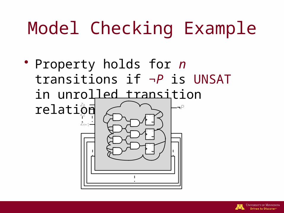
Model Checking Example
• Property holds for n transitions if ¬P is UNSAT in unrolled transition relation
Q
QSET
CLR
D
Q
QSET
CLR
D
Q
QSET
CLR
D
….
….
….
¬P
….
z0z1z2
zn+1
….

Model Checking Example
• Property holds for n transitions if ¬P is UNSAT in unrolled transition relation
Q
QSET
CLR
D
Q
QSET
CLR
D
Q
QSET
CLR
D…. …
.¬P'
….
x0x1x2
xm+1
….
z00
z10
z20
zn+10
….
x0'
….
x1'
x2'
xm+1'

Model Checking Example
• Property holds for n transitions if ¬P is UNSAT in unrolled transition relation
Q
QSET
CLR
D
Q
QSET
CLR
D
Q
QSET
CLR
D….
¬P1
….
x0x1x2
xm+1
….
z00
z10
z20
zn+10
….

Model Checking Example
• Property holds for n transitions if ¬P is UNSAT in unrolled transition relation
Q
QSET
CLR
D
Q
QSET
CLR
D
Q
QSET
CLR
D….
….
¬P1
….
Q
QSET
CLR
D
Q
QSET
CLR
D
Q
QSET
CLR
D….
¬P2
….
z01
z11
z21
zn+11
….
x0x1x2
xm+1
….
z00
z10
z20
zn+10
….

Model Checking Example
• Property holds for n transitions if ¬P is UNSAT in unrolled transition relation
Q
QSET
CLR
D
Q
QSET
CLR
D
Q
QSET
CLR
D….
….
¬P1
….
Q
QSET
CLR
D
Q
QSET
CLR
D
Q
QSET
CLR
D….
….
¬P2
….
z01
z11
z21
zn+11
….
x0x1x2
xm+1
….
Q
QSET
CLR
D
Q
QSET
CLR
D
Q
QSET
CLR
D….
….
z02
z12
z22
zn+12
….
¬P3z0
0
z10
z20
zn+10
….

What is PDR?
• Property Directed Reachability (PDR)– New symbolic model checking algorithm– Solves individual frames in isolation
• Advantages over other algorithms– SAT-Based not BDD-Based– No need for long unrollings– No spurious counter examples

How does PDR work?
• The trace contains sets of clauses Fi called frames.
• Frame Fi symbolically represents over approximation of states reachable in i transitions.

How Does PDR Work?
Q
QSET
CLR
D
Q
QSET
CLR
D
Q
QSET
CLR
D….
….
¬P1
….
Q
QSET
CLR
D
Q
QSET
CLR
D
Q
QSET
CLR
D….
….
¬P2
….
z01
z11
z21
zn+11
….
x0x1x2
xm+1
….
Q
QSET
CLR
D
Q
QSET
CLR
D
Q
QSET
CLR
D….
….
z02
z12
z22
zn+12
….
¬P3z0
0
z10
z20
zn+10
….
CNF formula: T 0 CNF formula: T 1 CNF formula: T 2

How Does PDR Work?
Q
QSET
CLR
D
Q
QSET
CLR
D
Q
QSET
CLR
D….
….
¬P1
….
Q
QSET
CLR
D
Q
QSET
CLR
D
Q
QSET
CLR
D….
….
¬P2
….
z01
z11
z21
zn+11
….
x0x1x2
xm+1
….
Q
QSET
CLR
D
Q
QSET
CLR
D
Q
QSET
CLR
D….
….
z02
z12
z22
zn+12
….
¬P3z0
0
z10
z20
zn+10
….
SAT?: T 2 ˄ ¬P’
Result: x1x2x3x4
SAT?: T 1 ˄ x’1x’
2x’3x’
4
Result: x1x2x3x4
SAT?: I ˄ T 0 ˄ x’1x’
2x’3x’
4
Result: UNSAT!

Q
QSET
CLR
D
Q
QSET
CLR
D
Q
QSET
CLR
D…. …
.
¬P'
….
x0x1x2
xm+1
….
z00
z10
z20
zn+10
….
x0'
….
x1'
x2'
xm+1'
How Does PDR Work?
¬PI
SAT?: Fi ˄ T ˄ ¬P’
SAT?: Fi-1 ˄ T ˄ x’1x’
2x’3x’
4
x1x2x3x4
F0
x1x2x3x4
x1x2x4
x1x2x3x4
Next StatePrev State
x1x2x3
x1x2x3x4
Cube Reduction!
Fi
CNF formula: T

How to improve PDR
• PDR requires small cubes to be effective– Reductions via Ternary Valued Simulation– Reductions via MUC inspection
• Idea: The use of non-state variables may yield smaller cubes

Intuition for Non-State VariablesFi-1
Fi
Three cubes in terms of x0x1x2x3 blocked by one cube in terms of g0g1!

Shifting the Transition Relation
Fi-1 Fi

Shifting the Transition Relation
Fi-1 Fi

Shifting the Transition Relation
Fi-1 Fi

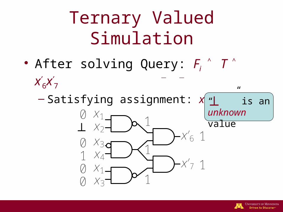
Ternary Valued Simulation
• After solving Query: Fi ˄ T ˄ x’6x’
7
– Satisfying assignment: x1x2x3x4
x1x2
x3x4
x1x3
0
0
00
1
11
1x’6
x’7
1
1
1
┴“ ” is an unknown value

Ternary Valued Simulation
• After solving Query: Fi ˄ T ˄ x’6x’
7
– Satisfying assignment: x1x2x3x4
x1x2
x3x4
x1x3
┴
0
┴0
1
11
┴x’6
x’7
┴
1
1
┴“ ” is an unknown value

Ternary Valued Simulation
• After solving Query: Fi ˄ T ˄ x’6x’
7
– Satisfying assignment: x1x2x3x4
x1x2
x3x4
x1x3
0
0
00
1
11
1x’6
x’7
1
1
1
┴“ ” is an unknown value
Ternary Valued Simulation
• After solving Query: Fi ˄ T ˄ x’6x’
7
– Satisfying assignment: x1x2x3x4
x1x2
x3x4
x1x3
0
0
00
┴
11
1x’6
x’7
1
1
1
┴“ ” is an unknown value

Ternary Valued Simulation
• After solving Query: Fi ˄ T ˄ x’6x’
7
– Satisfying assignment: x1x2x3x4
x1x2
x3x4
x1x3
0
┴
0┴
┴
1┴
┴x’6
x’7
1
1
┴
┴“ ” is an unknown value

Ternary Valued Simulation
• After solving Query: Fi ˄ T ˄ x’6x’
7
– Satisfying assignment: x1x2x3x4
x1x2
x3x4
x1x3
0
0
00
┴
11
1x’6
x’7
1
1
1
┴“ ” is an unknown value

Ternary Valued Simulation
• After solving Query: Fi ˄ T ˄ x’6x’
7
– Satisfying assignment: x1x2x3x4
x1x2
x3x4
x1x3
0
0
00
┴
┴ ┴
┴x’6
x’7
1
1
┴
┴“ ” is an unknown value

Ternary Valued Simulation
• After solving Query: Fi ˄ T ˄ x’6x’
7
– Satisfying assignment: x1x2x3x4
– Cube reduced: x1x3x4
x1x2
x3x4
x1x3
0
0
00
┴
11
1x’6
x’7
1
1
1
┴“ ” is an unknown value

Ternary Sim with Gate Vars
• Slightly more complex because of variable dependence
• Algorithm:– Order variables ascending by logic level– If the variables value is determined by
fanins: remove it– Otherwise try setting to: ┴

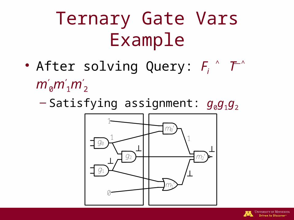
Ternary Gate Vars Example
• After solving Query: Fi ˄ T ˄ m’0m’
1m’2
– Satisfying assignment: g0g1g2
g0
g1
g2
m0'
m1'
m2'
0
1
1
1
1
1
1
0

Ternary Gate Vars Example
• After solving Query: Fi ˄ T ˄ m’0m’
1m’2
– Satisfying assignment: g0g1g2
g0
g1
g2
m0'
m1'
m2'
0
1
┴
┴1
┴
1
┴

Ternary Gate Vars Example
• After solving Query: Fi ˄ T ˄ m’0m’
1m’2
– Satisfying assignment: g0g1g2
g0
g1
g2
m0'
m1'
m2'
0
1
1
1
1
1
1
0
Ternary Gate Vars Example
• After solving Query: Fi ˄ T ˄ m’0m’
1m’2
– Satisfying assignment: g0g1g2
g0
g1
g2
m0'
m1'
m2'
0
1
1
┴
┴
1
┴
┴
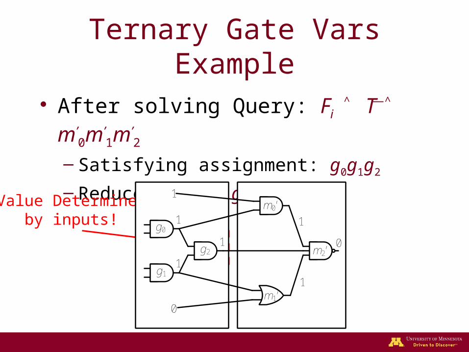
Ternary Gate Vars Example
• After solving Query: Fi ˄ T ˄ m’0m’
1m’2
– Satisfying assignment: g0g1g2
– Reduced Cube: g0g1
g0
g1
g2
m0'
m1'
m2'
0
1
1
1
1
1
1
0
Value Determinedby inputs!

Experimental Setup
• Ternary sim run twice: only gate vars and only state vars
• Vars are removed from cube by logic level and by priority
• After both passes the smaller cube is chosen

SAT Results

UNSAT Results
… … … … … … … …

Discussion
• Extension seems to work well for satisfiable benchmarks
• Does not seem to work as well for unsatisfiable benchmarks
• Randomness also affects the results.

Other Things We Tried
• Probabilistically chose gate variables• Used simulated annealing type
approach that gradually changed from gate cubes to state cubes
• Placed limits on max height of logic level used

Synthesizing Cyclic Dependencies with Craig Interpolation
Cyclic Combinational
Circuits
Reduction of Interpolants
Resolution ProofsProperty Directed
Reachability
Interpolation-Based Synthesis
Proof Manipulation
Formal Verification

Craig Interpolation
• Given formulas A and B such that A → ¬B, there exists I such that A → I → ¬B– I only contains variables that are
present in both A and B.
A
I
B

Craig Interpolation Cont.
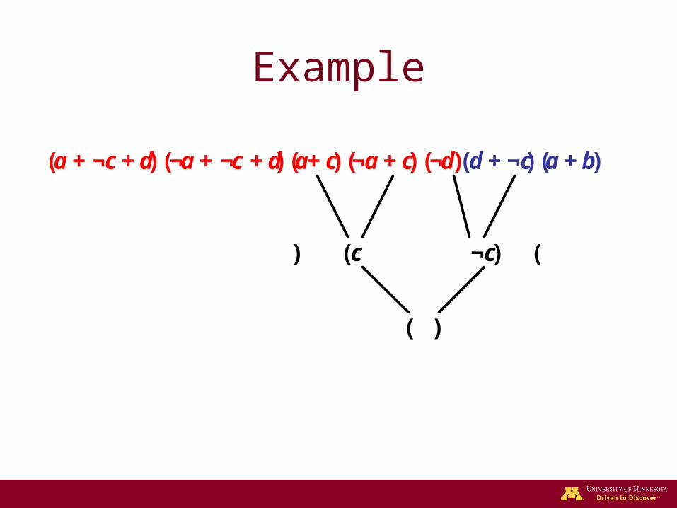
• For an instance of unsatisfiablity, if the clauses are divided into sets A and B then A → ¬B.– An interpolant I can be generated from a
proof of unsatisfiability of A and B.– The structure of this proof influences the
structure of I

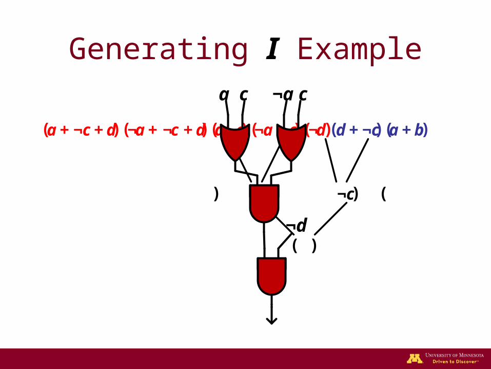
Generating I Example
(a + ¬c + d)(¬a + ¬c + d)(a+ c)(¬a + c)(¬d)(d + ¬c)(a + b)
(c) (¬c)
( )

Generating I Example
(a + ¬c + d)(¬a + ¬c + d)(a+ c)(¬a + c)(¬d)(d + ¬c)(a + b)
(c) (¬c)
( )

Generating I Example
(a+ c)(¬a + c)(¬d)(d + ¬c)
(c) (¬c)
( )

Generating I Example
(a+ c)(¬a + c)(¬d)(d + ¬c)
(c) (¬c)
( )
a c ¬a c

Generating I Example
)(¬d)(d + ¬c)
(c) (¬c)
( )
a c ¬a c

Generating I Example
(¬d)
(c) (¬c)
( )
a c ¬a c

Generating I Examplea c ¬a c
¬d
( )
(¬d)

Generating I Examplea c ¬a c
¬d
I(a,c)
A
I
B

Applications• Model Checking1
– Interpolants are used to over approximate the set of reachable states in a transition relation.
• Functional Dependencies2
– Interpolants are used to generate a dependency function in terms of a specified support set.
– The size of the interpolant directly correlates to the size of the circuit implementation.
1(K. L. McMillan. Interpolation and SAT-based model checking. ICCAV, 2003.)2C.-C. Lee, J.-H. R. Jiang, C.-Y. Huang, and A. Mishchenko. Scalable exploration of functional dependency by interpolation and incremental SAT solving. ICCAD, 2007.

Cyclic Circuit: 2 functions, 5 variables, 2 fan-in 4 gates.
cgab decf
cdeabf decabg
a
bc
c
de
Acyclic Circuit: at least 3 fan-in 4 gates.
a b c
c d e
f
g
Cyclic Combinational Circuits

How can one make a cyclic circuit?
Acyclic
f0 f1 f2
b ca d
f0 f1 f2
b ca d
f0
f2f1
a c
a b
c d
Consider some acyclic circuit
Pick support variables
Pick target support sets in a cyclic fashion

What is wrong with the old approach?
• Old method uses BDDs.– These do not scale well with circuit size.
• Old method for functional dependencies relies on algebraic manipulation.– Also does not scale well with circuit size.

What is better with the new approach
• Uses SAT-based method for functional dependency.
• SAT-based cyclic analysis during synthesis.– This scales better for larger circuits.

Functional Dependency
a b c f0 f1
0 0 0 1 1
0 0 1 0 1
0 1 0 0 0
0 1 1 1 0
1 0 0 0 0
1 0 1 0 1
1 1 0 0 0
1 1 1 1 0
• Two functions of three variables.
• For every assignment of f0 and c, there is a unique value for f1.
• This is necessary and sufficient to express f1 in terms of f0 and c.

Functional Dependency
a b c f0 f1
0 0 0 1 1
0 0 1 0 1
0 1 0 0 0
0 1 1 1 0
1 0 0 0 0
1 0 1 0 1
1 1 0 0 0
1 1 1 1 0
• Two functions of three variables.
• For every assignment of f0 and c, there is a unique value for f1.
• This is necessary and sufficient to express f1 in terms of f0 and c.

Functional Dependency
a b c f0 f1
0 0 0 1 1
0 0 1 0 1
0 1 0 0 0
0 1 1 1 0
1 0 0 0 0
1 0 1 0 1
1 1 0 0 0
1 1 1 1 0
• Two functions of three variables.
• For every assignment of f0 and c, there is a unique value for f1.
• This is necessary and sufficient to express f1 in terms of f0 and c.

Functional Dependency
a b c f0 f1
0 0 0 1 1
0 0 1 0 1
0 1 0 0 0
0 1 1 1 0
1 0 0 0 0
1 0 1 0 1
1 1 0 0 0
1 1 1 1 0
• Two functions of three variables.
• For every assignment of f0 and c, there is a unique value for f1.
• This is necessary and sufficient to express f1 in terms of f0 and c.

Functional Dependency
a b c f0 f1
0 0 0 1 1
0 0 1 0 1
0 1 0 0 0
0 1 1 1 0
1 0 0 0 0
1 0 1 0 1
1 1 0 0 0
1 1 1 1 0
• Two functions of three variables.
• For every assignment of f0 and c, there is a unique value for f1.
• This is necessary and sufficient to express f1 in terms of f0 and c.

Functional Dependency
• Two functions of three variables.
• For every assignment of f0 and c, there is a unique value for f1.
• This is necessary and sufficient to express f1 in terms of f0 and c.
a b c f0 f1
0 0 0 1 1
0 0 1 0 1
0 1 0 0 0
0 1 1 1 0
1 0 0 0 0
1 0 1 0 1
1 1 0 0 0
1 1 1 1 0
c f0 f1
0 0 0
0 1 1
1 0 1
1 1 0

Functional Dependency• C.-C. Lee, J.-H. R. Jiang, C.-Y. Huang, and A. Mishchenko, “Scalable
exploration of functional dependency by interpolation and incremental SAT solving”, ICCAD ‘07
If SAT, the dependency function h does not exist.
If UNSAT, Craig Interpolation can be used to derive an expression for h.
f0 Left
f0 f1 f2 f3
x0 x1 xn
f0 ≠ f0*
f0 Right
f3* f2* f1* f0*
x0*x1* xn*
f2 = f2* f3 = f3* f1 = f1*
g1
SAT?
. . . . . .
Tells us if f0 (x0, x1, … , xn) can be expressed in terms of some function h (f0, f1, f2, f3)
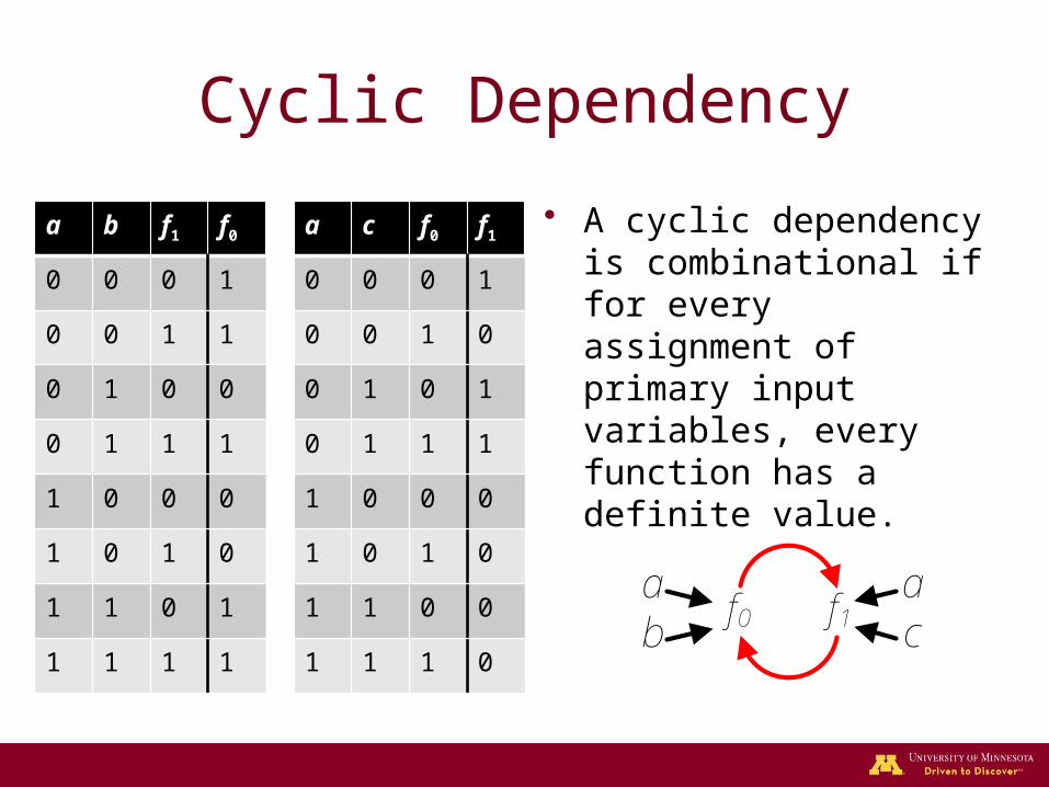
Cyclic Dependency
• A cyclic dependency is combinational if for every assignment of primary input variables, every function has a definite value.
a b f1 f0
0 0 0 1
0 0 1 1
0 1 0 0
0 1 1 1
1 0 0 0
1 0 1 0
1 1 0 1
1 1 1 1
a c f0 f1
0 0 0 1
0 0 1 0
0 1 0 1
0 1 1 1
1 0 0 0
1 0 1 0
1 1 0 0
1 1 1 0
f0 f1ab
ac
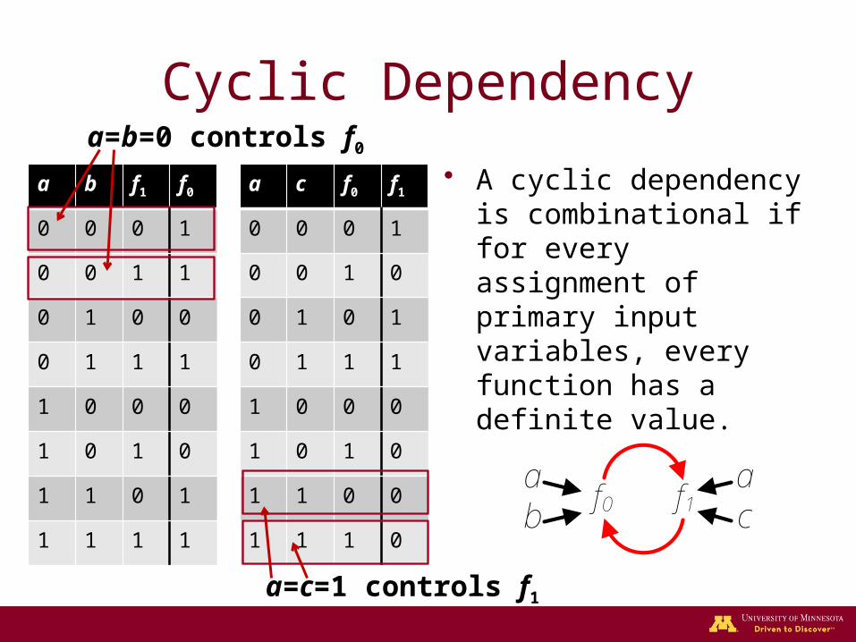
Cyclic Dependency
• A cyclic dependency is combinational if for every assignment of primary input variables, every function has a definite value.
a b f1 f0
0 0 0 1
0 0 1 1
0 1 0 0
0 1 1 1
1 0 0 0
1 0 1 0
1 1 0 1
1 1 1 1
a c f0 f1
0 0 0 1
0 0 1 0
0 1 0 1
0 1 1 1
1 0 0 0
1 0 1 0
1 1 0 0
1 1 1 0
a=b=0 controls f0
a=c=1 controls f1
f0 f1ab
ac

Cyclic Dependency
• A cyclic dependency is combinational if for every assignment of primary input variables, every function has a definite value.
a b f1 f0
0 0 0 1
0 0 1 1
0 1 0 0
0 1 1 1
1 0 0 0
1 0 1 0
1 1 0 1
1 1 1 1
a c f0 f1
0 0 0 1
0 0 1 0
0 1 0 1
0 1 1 1
1 0 0 0
1 0 1 0
1 1 0 0
1 1 1 0
a=c=0, b=1 controls neither!
f0 f1ab
ac

Cyclic Dependency
• The circuit is not combinational if three conditions are satisfied1. All primary input variables
the same in each row.
2. Controlling values are propagated.
3. Some function is toggling.
a b f1 f0
0 0 0 1
0 0 1 1
0 1 0 0
0 1 1 1
1 0 0 0
1 0 1 0
1 1 0 1
1 1 1 1
a c f0 f1
0 0 0 1
0 0 1 0
0 1 0 1
0 1 1 1
1 0 0 0
1 0 1 0
1 1 0 0
1 1 1 0
a=c=0, b=1 controls neither!
f0 f1ab
ac

Cyclic Dependency• Create a SAT instance
that satisfies three conditions.
• A Left and a Right copy of each dependency function.– Each copy considers one
row of the truth table.f0 Left f0 Right f1 Left f1 Right
a b f1L a b f1
R a c f0L a c f0
R
f0 f0* f1 f1
*
Condition 3
(f0 + f0* + f0
L)(f0 + f0* + f0
R)(f0 + f0
* + f0L)(f0 + f0
* + f0R)
(f1 + f1* + f1
L)(f1 + f1* + f1
R)(f1 + f1
* + f1L)(f1 + f1
* + f1R)
Condition 2
Condition 1
SAT?
f0 f1ab
ac

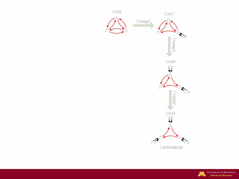
Synthesizing Cyclic Dependencies
1. Select a candidate set of target functions and support sets.
2. Generate their implementations via Craig Interpolation.
3. Use branch and bound search to pick solution.
4. Use SAT to verify if solution is combinational.
f0
f1 f2
Cost 6

Change f2
f0
f1 f2
Cost 6
f0
f1 f2
c d
Cost 7

Change f2
Change f0
f0
f1 f2
Cost 6
f0
f1 f2
c d
Cost 7
Cost 8
c d
f0
f1 f2
a b
Change f2
Change f0
Change f1
f0
f1 f2
Cost 6
f0
f1 f2
c d
Cost 7
Cost 8
Cost 9
c d
f0
f1 f2
a b
c d
f0
f1 f2
a b
c d
Combinational!

Change f2
Change f0
Change f1
f0
f1 f2
Cost 6
f0
f1 f2
c d
Cost 7
Cost 8
Cost 9
c d
f0
f1 f2
a b
c d
f0
f1 f2
a b
c d
Combinational!
. . .
. . .
Change f0
Chang
e f 2

Change f2
Change f0
Change f1
f0
f1 f2
Cost 6
f0
f1 f2
c d
Cost 7
Cost 8
Cost 9
c d
f0
f1 f2
a b
c d
f0
f1 f2
a b
c d
Combinational!
. . .
. . .
. . .
. . .
Change f0
Chang
e f 2
Change f2
Cha
nge
f 1

Change f2
Change f0
Change f1
f0
f1 f2
Cost 6
f0
f1 f2
c d
Cost 7
Cost 8
Cost 9
c d
f0
f1 f2
a b
c d
f0
f1 f2
a b
c d
f0
f1 f2
Cost 7
a b
Combinational!
Change f0
. . .
. . .
. . .
. . .
Change f0
Chang
e f 2
Change f2
Cha
nge
f 1

Change f2
Change f0
Change f1
f0
f1 f2
Cost 6
f0
f1 f2
c d
Cost 7
Cost 8
Cost 9
c d
f0
f1 f2
a b
c d
f0
f1 f2
a b
c d
f0
f1 f2
Cost 7
a b
f0
f1 f2
Cost 8
a b c d
Combinational!
Change f0
Change f0
. . .
. . .
. . .
. . .
Change f0
Chang
e f 2
Change f2
Cha
nge
f 1

Change f2
Change f0
Change f1
f0
f1 f2
Cost 6
f0
f1 f2
c d
Cost 7
Cost 8
Cost 9
c d
f0
f1 f2
a b
c d
f0
f1 f2
a b
c d
f0
f1 f2
Cost 7
a b
f0
f1 f2
Cost 8
a b c d
f0
f1 f2
Cost 9
a b c d
Combinational! Combinational!
Change f0
Change f0
Change f2
c d
. . .
. . .
. . .
. . .
Change f0
Chang
e f 2
Change f2
Cha
nge
f 1

Change f2
Change f0
Change f1
f0
f1 f2
Cost 6
f0
f1 f2
c d
Cost 7
Cost 8
Cost 9
c d
f0
f1 f2
a b
c d
f0
f1 f2
a b
c d
f0
f1 f2
Cost 7
a b
f0
f1 f2
Cost 8
a b c d
f0
f1 f2
Cost 9
a b c d
Combinational! Combinational!
Change f0
Change f0
Change f2
c d
. . .
. . .
. . .
. . .
. . .
Change f1
Change f0
Chang
e f 2
Change f2
Cha
nge
f 1

Change f2
Change f0
Change f1
f0
f1 f2
Cost 6
f0
f1 f2
c d
Cost 7
Cost 8
Cost 9
c d
f0
f1 f2
a b
c d
f0
f1 f2
a b
c d
f0
f1 f2
Cost 7
a b
f0
f1 f2
Cost 8
a b c d
f0
f1 f2
Cost 9
a b c d
Combinational! Combinational!
Change f0
Change f0
Change f2
c d
. . .
. . .
. . .
. . .
. . .
. . .
. . .
Change f1
Change f0
Chang
e f 2
Change f1Change f2
Change f2
Cha
nge
f 1

Change f2
Change f0
Change f1
f0
f1 f2
Cost 6
f0
f1 f2
c d
Cost 7
Cost 8
Cost 9
c d
f0
f1 f2
a b
c d
f0
f1 f2
a b
c d
f0
f1 f2
Cost 7
a c
f0
f1 f2
Cost 7
a b
f0
f1 f2
Cost 8
a b c d
f0
f1 f2
Cost 9
a b c d
Combinational! Combinational!
Change f1
Change f0
Change f0
Change f2
c d
. . .
. . .
. . .
. . .
. . .
. . .
. . .
Change f1
Change f0
Chang
e f 2
Change f1Change f2
Change f2
Cha
nge
f 1

Change f2
Change f0
Change f1
f0
f1 f2
Cost 6
f0
f1 f2
c d
Cost 7
Cost 8
Cost 9
c d
f0
f1 f2
a b
c d
f0
f1 f2
a b
c d
f0
f1 f2
Cost 7
a c
f0
f1 f2
Cost 8
c d
a b
f0
f1 f2
Cost 7
a b
f0
f1 f2
Cost 8
a b c d
f0
f1 f2
Cost 9
a b c d
Combinational! Combinational!
Combinational!
Change f1
Change f0
Change f0
Change f0
Change f2
c d
. . .
. . .
. . .
. . .
. . .
. . .
. . .
Change f1
Change f0
Chang
e f 2
Change f1Change f2
Change f2
Cha
nge
f 1

Change f2
Change f0
Change f1
f0
f1 f2
Cost 6
f0
f1 f2
c d
Cost 7
Cost 8
Cost 9
c d
f0
f1 f2
a b
c d
f0
f1 f2
a b
c d
f0
f1 f2
Cost 7
a c
f0
f1 f2
Cost 8
c d
a b
f0
f1 f2
Cost 7
a b
f0
f1 f2
Cost 8
a b c d
f0
f1 f2
Cost 9
a b c d
Combinational! Combinational!
Combinational!
Change f1
Change f0
Change f0
Change f0
Change f2
c d
. . .
. . .
. . .
. . .
. . .
. . .
. . .
. . .
. . .
Change f1
Change f2
Change f1
Change f0
Chang
e f 2
Change f1Change f2
Change f2
Cha
nge
f 1
What are the problems with the new approach?
• The structure of the interpolants is relatively poor.
• Because of this, we use support set size as our cost function.– This can be a valid metric for FPGAs.

Reduction of Interpolants For Logic Synthesis
Cyclic Combinational
Circuits
Reduction of Interpolants
Resolution ProofsProperty Directed
Reachability
Interpolation-Based Synthesis
Proof Manipulation
Formal Verification
Generating I Example
(a + ¬c + d)(¬a + ¬c + d)(a+ c)(¬a + c)(¬d)(d + ¬c)(a + b)
(c) (¬c)
( )
a c ¬a c
¬d

a ¬c d ¬a ¬c d a c ¬a c
¬d
Generating I Example
(a + ¬c + d)(¬a + ¬c + d)(a+ c)(¬a + c)(¬d)(d + ¬c)(a + b)
(d + ¬c)
( )
(¬c) (c)

Generating I Examplea ¬c d ¬a ¬c d a c ¬a c
¬d
a c ¬a c
¬d>

Draw Backs
• Model Checking– Interpolants that are large over
approximations can trigger false state reachability.
• Functional Dependencies– In many cases the structure of the
interpolant may be very redundant and large.

Proposed Solution
• Goal: reduce size of an interpolant generated from a resolution proof.– Change the structure of a proof with the
aim of reducing interpolant size. – In general, the fewer intermediate nodes in
the proof, the smaller then interpolant.

Resolution Proofs
• A proof of unsatisfiability for an in instance of SAT forms a graph structure.
• The original clauses are called the roots and the empty clause is the only leaf.
• Every node in the graph (besides the roots) is formed via Boolean resolution.– I.e.: (c + d)(¬c + e) → (d + e)– Here “c” is referred to as the pivot variable.
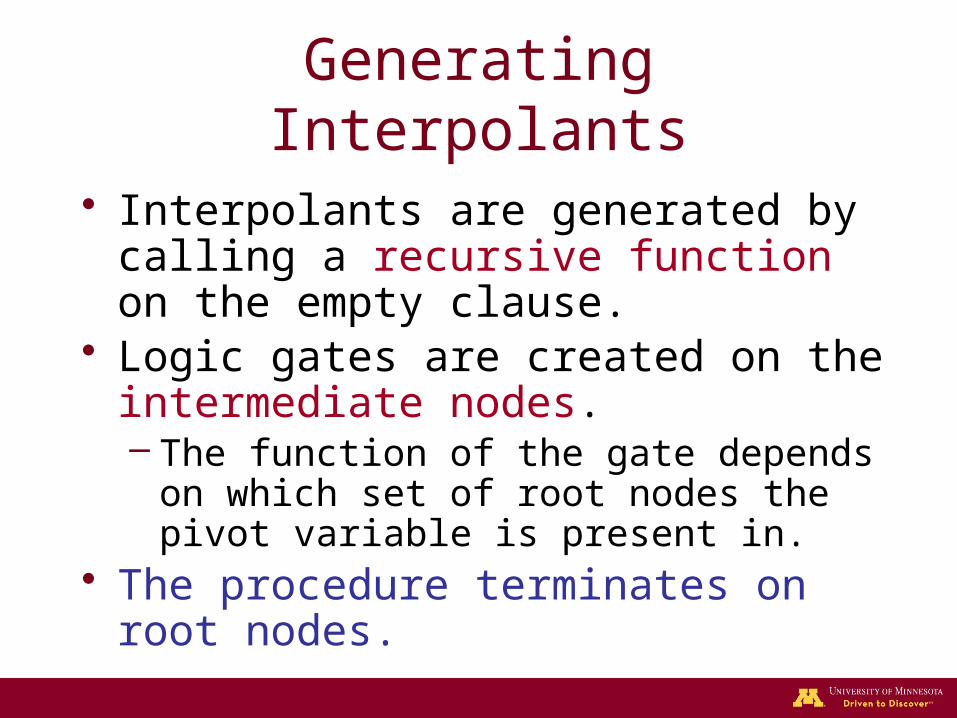
Generating Interpolants
• Interpolants are generated by calling a recursive function on the empty clause.
• Logic gates are created on the intermediate nodes.– The function of the gate depends on which
set of root nodes the pivot variable is present in.
• The procedure terminates on root nodes.

Proposition 1
• Nodes resolved only from A (or B) can be considered as roots of A (or B).
• Proof: Given clauses C, D, and E such that (C)(D) → (E), (C)(D) ≡ (C)(D)(E).
A
I
B
Example
(a + ¬c + d)(¬a + ¬c + d)(a+ c)(¬a + c)(¬d)(d + ¬c)(a + b)
(c) (¬c)
( )

Example
(a + ¬c + d)(¬a + ¬c + d)(a+ c)(¬a + c)(¬d)(d + ¬c)(a + b)
(c) (¬c)
( )
c ¬d

Example
(a + ¬c + d)(¬a + ¬c + d)(a+ c)(¬a + c)(¬d)(d + ¬c)(a + b)
(d + ¬c)
( )
(¬c) (c)

Example
(a + ¬c + d)(¬a + ¬c + d)(a+ c)(¬a + c)(¬d)(d + ¬c)(a + b)
(d + ¬c)
( )
(¬c) (c)
0
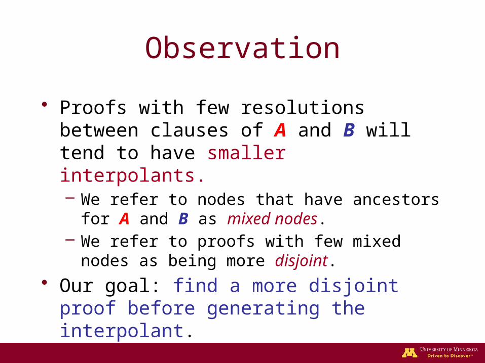
Observation
• Proofs with few resolutions between clauses of A and B will tend to have smaller interpolants.– We refer to nodes that have ancestors for A and B
as mixed nodes.– We refer to proofs with few mixed nodes as being
more disjoint.
• Our goal: find a more disjoint proof before generating the interpolant.

Proposition 2
• If node c in a proof is implied by root nodes R, then all assignments that satisfy the clauses of R also satisfy c
• Proof: since R → c, whenever R = 1, c = 1

SAT Based Methods
• Since R → c the SAT instance (R)(¬c) will be unsatisfiable.
• R. Gershman used this observation to find Minimum Unsatisfiable Cores (MUCs) for resolution proofs1.
1R. Gershman, M. Koifman, and O. Strichman. An approach for extracting a small unsatisfiable core. Formal Methods in System Design, 2008.

Example
• What if we want to know if (¬c) can be implied by A?
• Check the satisfiability of:(a + ¬c + d)(¬a + ¬c + d)(a+ c)(¬a + c)(¬d)(c)
Root of A?
(a + ¬c + d)(¬a + ¬c + d)(a+ c)(¬a + c)(¬d)(d + ¬c)(a + b)
(c) (¬c)
( )
= UNSAT!

Example
• What if we want to know if ( ) can be implied by A?
• Check the satisfiability of:
(a + ¬c + d)(¬a + ¬c + d)(a+ c)(¬a + c)(¬d)
Root of A?
(a + ¬c + d)(¬a + ¬c + d)(a+ c)(¬a + c)(¬d)(d + ¬c)(a + b)
(c) (¬c)
( )
= UNSAT!

Example
• What if we want to know if ( ) can be implied by A?
• Check the satisfiability of:
(a + ¬c + d)(¬a + ¬c + d)(a+ c)(¬a + c)(¬d)
Root of A?
(a + ¬c + d)(¬a + ¬c + d)(a+ c)(¬a + c)(¬d)(d + ¬c)(a + b)
(c) (¬c)
( )
= UNSAT!
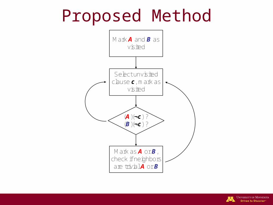
Proposed MethodMark A and B as
visited
Select unvisited clause c, mark as
visited
(A)(¬c) ?(B)(¬c) ?
Mark as A or B, check if neighbors are trivial A or B
Optimizations
• The complexity of this approach is dominated by solving different SAT instances.
• We can reduce the number of calls to the SAT solver by checking mixed nodes in specific orders.

Optimization 1
• If node 1 is a root of A (B) then we don’t need to check node 3.
...( )( )( )( )( )( )( )...
( 3 ) ( 4 ) ( 5 )
( 1 ) ( 2 )
( )
……..
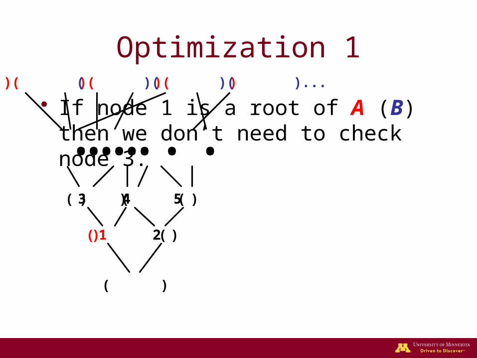
• If node 1 is a root of A (B) then we don’t need to check node 3.
...( )( )( )( )( )( )( )...
( 3 ) ( 4 ) ( 5 )
( 1 ) ( 2 )
( )
……..
Optimization 1

• If nodes 1 and 2 are roots of A (B) then we don’t need to check nodes 3 4 or 5.
...( )( )( )( )( )( )( )...
( 3 ) ( 4 ) ( 5 )
( 1 ) ( 2 )
( )
……..
Optimization 1

• If nodes 1 and 2 are roots of A (B) then we don’t need to check nodes 3 4 or 5.
...( )( )( )( )( )( )( )...
( 3 ) ( 4 ) ( 5 )
( 1 ) ( 2 )
( )
……..
Optimization 1
Checking nodes near the leaf first is a backward search
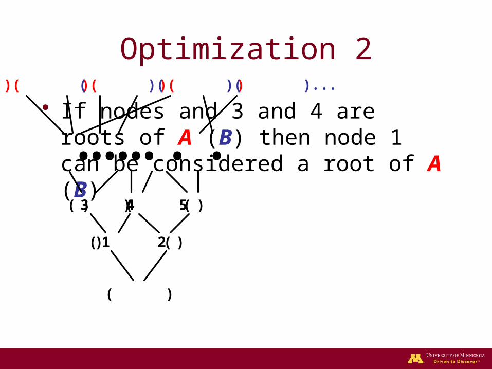
• If nodes and 3 and 4 are roots of A (B) then node 1 can be considered a root of A (B)
...( )( )( )( )( )( )( )...
( 3 ) ( 4 ) ( 5 )
( 1 ) ( 2 )
( )
……..
Optimization 2

• If nodes and 3 and 4 are roots of A (B) then node 1 can be considered a root of A (B)
...( )( )( )( )( )( )( )...
( 3 ) ( 4 ) ( 5 )
( 1 ) ( 2 )
( )
……..
Optimization 2

• If nodes and 3 and 4 are roots of A (B) then node 1 can be considered a root of A (B)
...( )( )( )( )( )( )( )...
( 3 ) ( 4 ) ( 5 )
( 1 ) ( 2 )
( )
……..
Optimization 2
Checking nodes near the roots first is a forward search
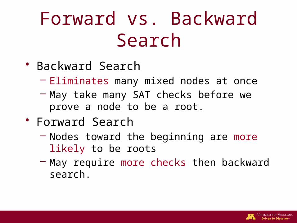
Forward vs. Backward Search
• Backward Search– Eliminates many mixed nodes at once– May take many SAT checks before we prove a
node to be a root.
• Forward Search– Nodes toward the beginning are more likely to be
roots– May require more checks then backward search.

Incremental Techniques
• Each call to the SAT solver is very similar.– Each instance is in the form (A)(¬c) or (B)(¬c).
• The negated literals of clause c can be set as unit assumptions to the SAT Solver.– We then just solve the same instance
repeatedly with different assumptions.
• Variables aoff and boff can be added to the clauses of A and B respectively.

Example
• What if we want to know if (d + ¬c) can be implied by A?
• Assume aoff = 0, boff = 1, d = 0, and c = 1. Then check the satisfiability of:
(a + ¬c + d + aoff)(¬a + ¬c + d + aoff)(a+ c + aoff)(¬a + c + aoff) (¬d + aoff)(d + ¬c + boff)(a + b + boff)
Root of A?
(a + ¬c + d)(¬a + ¬c + d)(a+ c)(¬a + c)(¬d)(d + ¬c)(a + b)
(c) (¬c)
( )
= UNSAT!

Experiment
• Searched for different functional dependencies in benchmark circuits.– Found small support sets for POs expressed in
terms of other POs and PIs.
• Performed forward and backward search on the resolution proofs.– The number of SAT checks was limited to 2500.– This limit was reached for the larger proofs.

Experiment Cont.
• After the new interpolants from the modified resolution proofs are. generated, the size is compared to the un modified proofs.
• The size after running logic minimization on the modified and non modified interpolants is also compared.
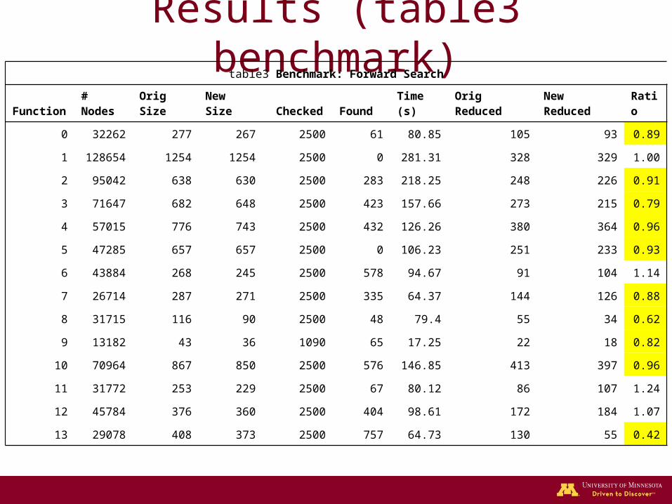
Results (table3 benchmark)table3 Benchmark: Forward Search
Function # Nodes Orig Size New Size Checked Found Time (s) Orig Reduced New Reduced Ratio
0 32262 277 267 2500 61 80.85 105 93 0.89
1 128654 1254 1254 2500 0 281.31 328 329 1.00
2 95042 638 630 2500 283 218.25 248 226 0.91
3 71647 682 648 2500 423 157.66 273 215 0.79
4 57015 776 743 2500 432 126.26 380 364 0.96
5 47285 657 657 2500 0 106.23 251 233 0.93
6 43884 268 245 2500 578 94.67 91 104 1.14
7 26714 287 271 2500 335 64.37 144 126 0.88
8 31715 116 90 2500 48 79.4 55 34 0.62
9 13182 43 36 1090 65 17.25 22 18 0.82
10 70964 867 850 2500 576 146.85 413 397 0.96
11 31772 253 229 2500 67 80.12 86 107 1.24
12 45784 376 360 2500 404 98.61 172 184 1.07
13 29078 408 373 2500 757 64.73 130 55 0.42

Results (table3 benchmark)table3 Benchmark: Backward Search
Function Nodes Orig Size New Size Checked Found Time (s) Orig Reduced New Reduced Ratio
0 32262 277 129 2500 20 85.88 105 58 0.55
1 128654 1254 1238 2500 5 287.62 328 346 1.05
2 95042 638 574 2500 8 225.37 248 217 0.88
3 71647 682 469 2500 45 179.96 273 177 0.65
4 57015 776 490 2500 26 144.83 380 193 0.51
5 47285 657 611 2500 8 114.33 251 242 0.96
6 43884 268 224 2500 8 107.96 91 106 1.16
7 26714 287 87 2500 27 76.61 144 51 0.35
8 31715 116 76 2500 15 85.23 55 34 0.62
9 13182 43 36 1017 3 16.55 22 18 0.82
10 70964 867 349 2500 41 179.22 413 192 0.46
11 31772 253 191 2500 8 82.38 86 50 0.58
12 45784 376 203 2500 34 120 172 117 0.68
13 29078 408 112 2500 32 84.29 130 37 0.28

Results (Summarized)Forward Search
Benchmark Nodes Checked Found % Change % Change Reduced Time (s)
apex1 28279 2413 30 -4.89% -2.73% 69.48
apex3 68585 1494 21 -2.12% -1.47% 140.99
styr 9373 2143 88 -8.71% -5.71% 18.3
s1488 5748 824 29 -9.24% -8.41% 7.62
s1494 10488 1266 21 -6.69% -4.43% 15.51
s641 46416 1886 39 -26.67% -2.33% 97.45
s713 42412 1910 89 -36.00% -3.70% 89.16
table5 35373 2500 252 -13.83% -4.08% 48.05
vda 12951 2011 120 -18.78% -17.33% 27.34
sbc 13951 1094 8 -1.46% -1.08% 19.09

Results (Summarized)Backward Search
Benchmark Nodes Checked Found % Change % Change Reduced Time (s)
apex1 28279 2384 6 -8.95% -5.84% 72.03
apex3 68585 1485 5 -8.41% -5.24% 145.63
styr 9373 2124 10 -11.57% -10.14% 19.36
s1488 5748 797 5 -9.92% -9.59% 7.98
s1494 10488 1241 7 -6.93% -5.19% 15.83
s641 46416 1820 14 -42.22% -2.78% 95.37
s713 42412 1724 17 -43.90% -6.20% 82.86
table5 35373 2358 7 -26.67% -15.83% 81.16
vda 12951 1850 7 -21.72% -19.72% 27.07
sbc 13951 1087 1 -1.46% -0.92% 19.09

Summary of Thesis

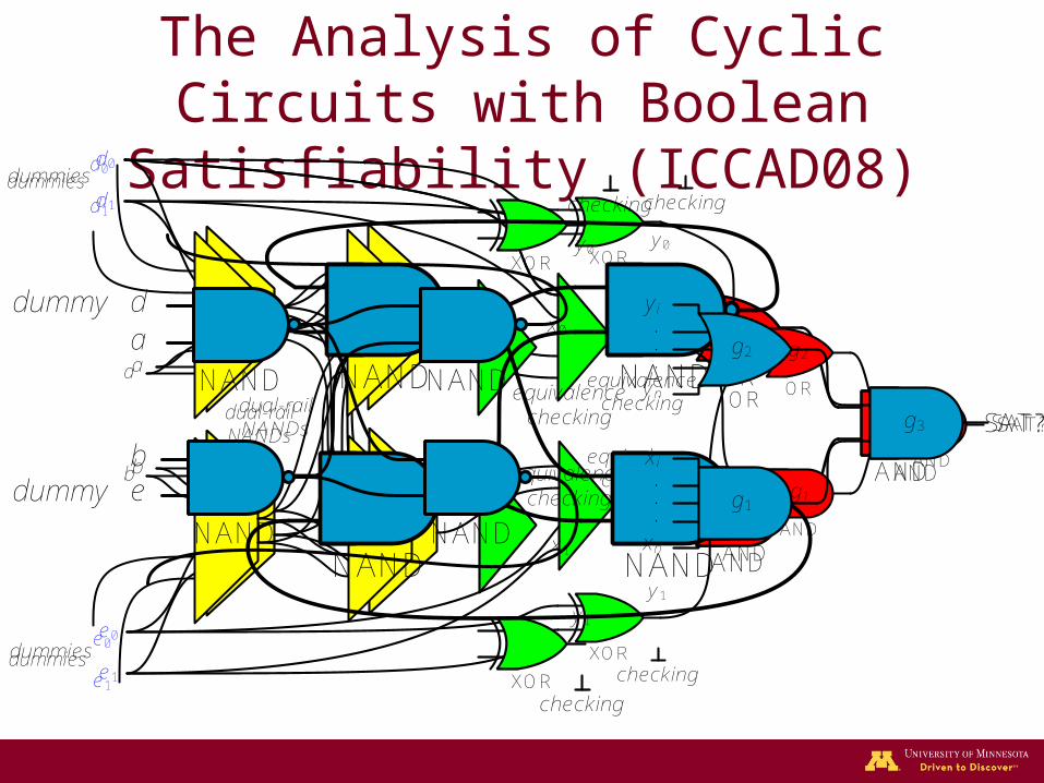
The Analysis of Cyclic Circuits with Boolean Satisfiability (ICCAD08)
• SAT-based algorithm for analyzing cyclic circuits on the gate level.
• Also work discussing mapping of cyclic circuits.

NAND
NAND
NAND
NAND
a
b
NAND
NAND
NAND
NAND
1
0
1
1
The Analysis of Cyclic Circuits with Boolean Satisfiability (ICCAD08)
AND
OR
AND
SAT?g3
g2
g1
AND
OR
AND
SAT?g3
g2
g1
XOR
XOR
b
a
e0
e1
d0
d1
equivalence checking
checking
equivalence checking
checking
dual-rail NANDs
dummies
dummies
y1
y0
x1
x0
b
a
e0
e1
d0
d1
dual-rail NANDs
dummies
dummiesXOR
XOR
equivalence checking
checking
equivalence checking
checking
y1
y0
x1
x0
NAND
NAND
NAND
NAND
a
b
AND
xi
xn
.
.
.
OR
yi
yn
.
.
.
AND
SAT?g3
g1
g2
NAND
NAND
NAND
NAND
a
b
d
e
dummy
dummy
The Analysis of Cyclic Circuits with Boolean Satisfiability (ICCAD08)

The Synthesis of Cyclic Dependencies with Craig Interpolation (IWLS09,
TODAES12)• Used SAT for functional level analysis• Craig Interpolation to generate the
dependencies• Branch and bound to find different
solutions

Acyclic
f0 f1 f2
b ca d
f0 f1 f2
b ca d
f0
f2f1
a c
a b
c d
Consider some acyclic circuit
Pick support variables
Pick target support sets in a cyclic fashion
The Synthesis of Cyclic Dependencies with Craig Interpolation (IWLS09,
TODAES12)

Reduction of Interpolants For Logic Synthesis (ICCAD10)
• Restructured resolution proofs to make smaller interpolants
• Used incremental SAT techniques to increase performance

(a + ¬c + d)(¬a + ¬c + d)(a+ c)(¬a + c)(¬d)(d + ¬c)(a + b)
(c) (¬c)
( )
(a + ¬c + d)(¬a + ¬c + d)(a+ c)(¬a + c)(¬d)(d + ¬c)(a + b)
(d + ¬c)
( )
(¬c) (c)
(a + ¬c + d)(¬a + ¬c + d)(a+ c)(¬a + c)(¬d)(d + ¬c)(a + b)
(d + ¬c)
( )
(¬c) (c)
0
Reduction of Interpolants For Logic Synthesis (ICCAD10)
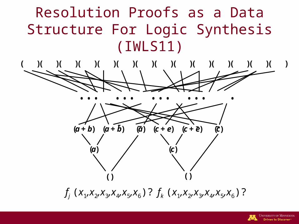
Resolution Proofs as a Data Structure For Logic Synthesis (IWLS11)
• Advocated using resolution proofs to perform large restructurings
• Showed that many nodes can be shared among similar proofs

fj (x1,x2,x3,x4,x5,x6)? fk (x1,x2,x3,x4,x5,x6)?
(a + b) (a + b) (a)
(a)
( )
…….. ……..(c + e) (c + e) (c)
(c)
( )
( )( )( )( )( )( ) ( )( )( )( )( )( )( )
Resolution Proofs as a Data Structure For Logic Synthesis (IWLS11)

fj (x1,x2,x3,x4,x5,x6)? fk (x1,x2,x3,x4,x5,x6)?
Resolution Proofs as a Data Structure For Logic Synthesis (IWLS11)
fj (x1,x2,x3,x4,x5,x6)? fk (x1,x2,x3,x4,x5,x6)?
( )( )( )( )( )( )( )( )( )( )( )( )( )( )
………….(a + b) (a + b) (a)
( )
(a)
(c + e) (c + e) (c)
(c)
( )
Resolution Proofs as a Data Structure For Logic Synthesis (IWLS11)

fj (x1,x2,x3,x4,x5,x6)? fk (x1,x2,x3,x4,x5,x6)?
Resolution Proofs as a Data Structure For Logic Synthesis (IWLS11)

• Extended PDR algorithm to use cubes of non-state variables
• Improved performance for satisfiable benchmarks
PDR and Gate Variables (DATE13)
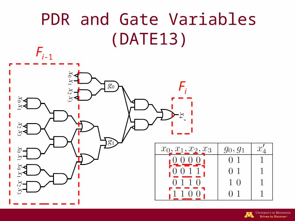
PDR and Gate Variables (DATE13)Fi-1
Fi

PI Vars
State VarsGate Vars
Next State Vars
PDR and Gate Variables (DATE13)

PI Vars Next Gate Vars
Gate Vars
PDR and Gate Variables (DATE13)

Future Directions

Cyclic Re-Writing
• DAG-Aware AIG Re-Writing is powerful for acyclic circuits– Uses pre-computed functions– Computes feasible cuts of the circuit
• Can re-writing be performed with cyclic circuits?

Cyclic Re-Writing Challenges
• After each cut is replaced combinational analysis must be performed– We can use SAT-Based analysis!
• Re-writing would require a database of good cyclic functions– Cyclic circuits implementing a single
function?

Single Output Cyclic Circuits
• Do there exists small cyclic circuits implementing a single function?
x0x1x2
xn-1
┴
f...

Single Output Cyclic Circuits
• Do there exists small cyclic circuits implementing a single function?
x0x1x2
xn-1
f...

Resolution Proofs and Interpolants
• Techniques may be extended to improve abstractions (over-approximations)
• Methods for generating good initial proofs (rather than quickly solving instances)

Property Directed Reachability
• The algorithm is very young• New heuristics for cube minimization• Possible extensions to probabilistic
model checking

Future Plans

Resolution Proofs as a Universal Data Structure for
Logic Synthesis

Data Structures
• Sum of Products (SOPs)– Advantages: explicit, readily mapable.– Disadvantages: not scalable.
• Binary Decision Diagrams (BDDs)– Advantages: canonical, easily manipulated.– Disadvantages: not readily mapable, not
scalable.

Data Structures
• And Inverter Graphs (AIGs)– Advantages:
• Compact.• Easily convertible to CNFs.• Scalable, efficient.
– Disadvantages:• Hard to perform large structural changes.

Resolution Proofs
• Implicitly extracted from SAT solvers; converted to logic via Craig Interpolation.
• Utilize as a data structure to perform logic manipulations.
• Advantages:– Scalable, efficient.– Can effect large structural changes.

AIG Synthesis• Re-writing
– Cuts are replaced by pre-computed optimal structures (Mishchenko ’06).
• SAT Sweeping– Nodes of an AIG can be merged by proven
equivalence (Zhu ‘06).• SAT-Based Resubstitution
– Target nodes are recomputed from other nodes (Lee ‘07).
AIG Synthesis
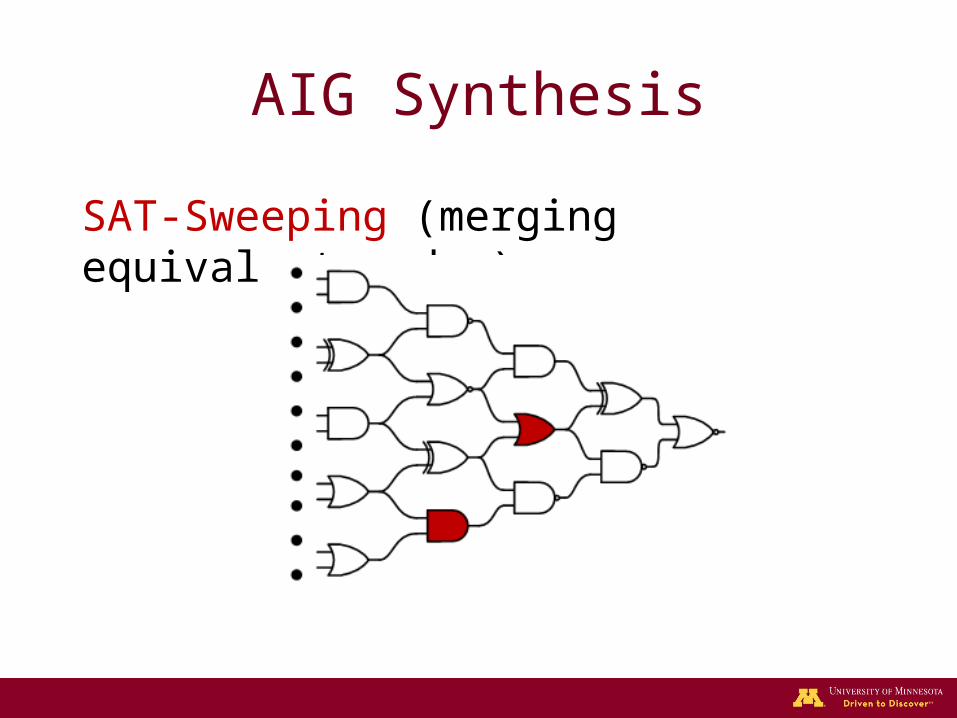
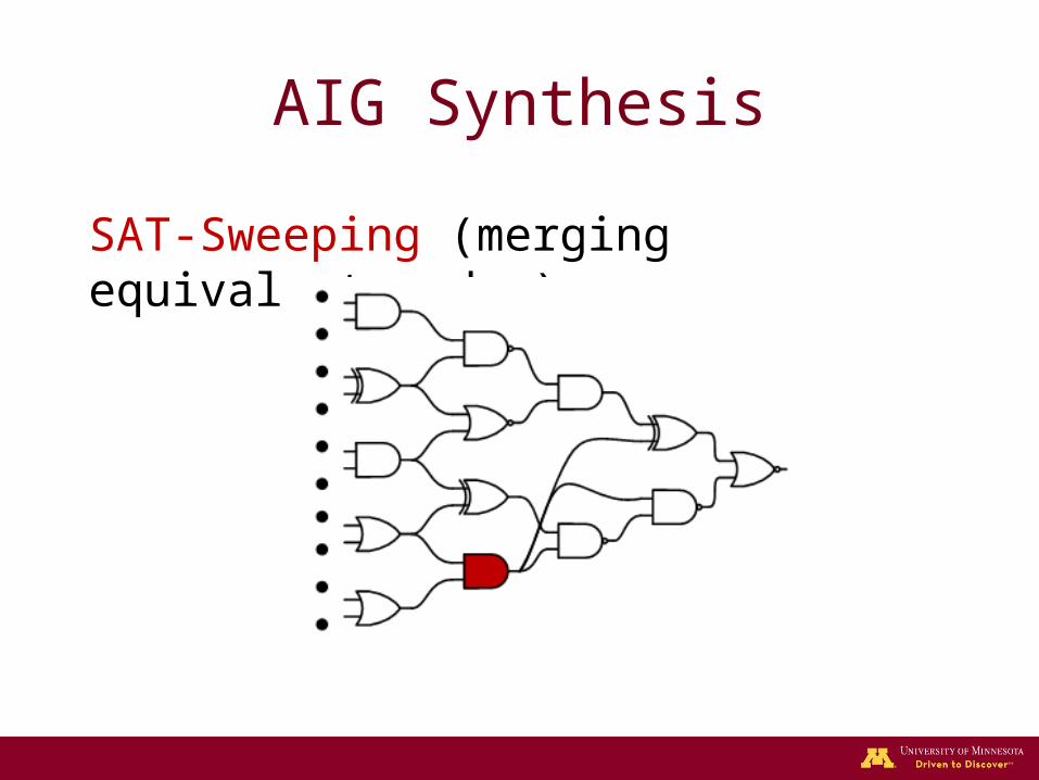
SAT-Sweeping (merging equivalent nodes)
AIG Synthesis
SAT-Sweeping (merging equivalent nodes)

AIG Synthesisz1 z2 zn
f1 fj-1 fj fk fk+1 fm
…………….
…. …. ….
• AIG re-writing– Local
manipulations performed on windows
– Local minimums can be reached

AIG Synthesisz1 z2 zn
f1 fj-1 fj fk fk+1 fm
…………….
…. …. ….
• AIG re-writing– Local
manipulations performed on windows
– Local minimums can be reached

AIG Synthesisz1 z2 zn
f1 fj-1 fj fk fk+1 fm
…………….
…. …. ….
• AIG re-writing– Local
manipulations performed on windows
– Local minimums can be reached

Resubstitution a.k.a. Functional Dependencies
Given target:
f (z1,z2,…,zn),
Given candidates:x1(z1,z2,…,zn), x2(z1,z2,…,zn), …, xm(z1,z2,…,zn)
is it possible to implement f (x1,x2,…,xm)?

Aig Synthesisz1 z2 zn
f1 fj-1 fj fk fk+1 fm
…………….
…. …. ….
x1
x2
f
• Resubstitution– f (x1,x2)?

Aig Synthesisz1 z2 zn
f1 fj-1 fj fk fk+1 fm
…………….
…. …. ….
x1
x2
f
• Resubstitution– f (x1,x2)?
– Large changes– This question is
formulated as a SAT instance.
– Craig Interpolation provides implementation.

Generating Multiple Dependencies
• Often, goal is to synthesize dependencies for multiple functions with overlapping support sets.
• In this case, multiple proofs are generated and then interpolated.
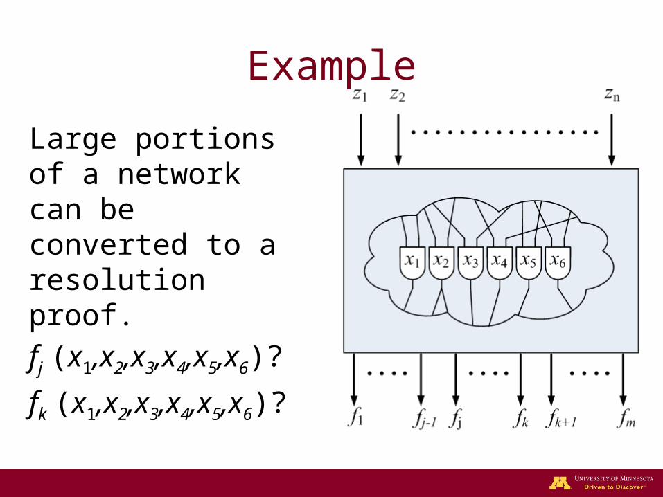
Example
Large portions of a network can be converted to a resolution proof.
fj (x1,x2,x3,x4,x5,x6)?
fk (x1,x2,x3,x4,x5,x6)?

Example
fj (x1,x2,x3,x4,x5,x6)? fk (x1,x2,x3,x4,x5,x6)?
(a + b) (a + b) (a)
(a)
( )
…….. ……..(c + e) (c + e) (c)
(c)
( )
( )( )( )( )( )( ) ( )( )( )( )( )( )( )

Example
fj (x1,x2,x3,x4,x5,x6)? fk (x1,x2,x3,x4,x5,x6)?
Observation
• There are often many ways to prove a SAT instance unsatisfiable.
• Same/similar nodes shared between different proofs.

Example
fj (x1,x2,x3,x4,x5,x6)? fk (x1,x2,x3,x4,x5,x6)?
( )( )( )( )( )( )( )( )( )( )( )( )( )( )
………….(a + b) (a + b) (a)
( )
(a)
(c + e) (c + e) (c)
(c)
( )

Example
fj (x1,x2,x3,x4,x5,x6)? fk (x1,x2,x3,x4,x5,x6)?

Restructuring Mechanism
• Some clause c can be resolved from some set of clauses W iff (W)(c) is unsatisfiable.
• The resolution proof of (W)(c) can be altered to show how c can be resolved from W.
(Gershman ‘08)

Example
Can (a + b) be resolved from (a + e + d)(a + b + d) (a + b + d + e)?
(a + b + c) (a + b + c) (a + e + d) (a + b + d) (a + b + d + e)
(a + b)
……………….
……………….
(Gershman ‘08)

Example
Can (a + b) be resolved from (a + e + d)(a + b + d) (a + b + d + e)?
(a) (b) (a + e + d) (a + b + d) (a + b + d + e)
(Gershman ‘08)

Example
Can (a + b) be resolved from (a + e + d)(a + b + d) (a + b + d + e)?
(a) (b) (a + e + d) (a + b + d) (a + b + d + e)
(e + d) (b + d) (b + d + e)
(Gershman ‘08)

Example
Can (a + b) be resolved from (a + e + d)(a + b + d) (a + b + d + e)?
(a) (b) (a + e + d) (a + b + d) (a + b + d + e)
(e + d) (b + d) (b + d + e)
(d) (d + e)
(Gershman ‘08)

Example
Can (a + b) be resolved from (a + e + d)(a + b + d) (a + b + d + e)?
(a) (b) (a + e + d) (a + b + d) (a + b + d + e)
(e + d) (b + d) (b + d + e)
(d) (d + e)
(d)
(Gershman ‘08)

Example
Can (a + b) be resolved from (a + e + d)(a + b + d) (a + b + d + e)?
(a) (b) (a + e + d) (a + b + d) (a + b + d + e)
(e + d) (b + d) (b + d + e)
(d) (d + e)
(d)( )
(Gershman ‘08)

Example
Can (a + b) be resolved from (a + e + d)(a + b + d) (a + b + d + e)?
(a) (b) (a + e + d) (a + b + d) (a + b + d + e)
(e + d) (b + d) (b + d + e)
(d) (d + e)
(d)(a + b)
(Gershman ‘08)

Example
Can (a + b) be resolved from (a + e + d)(a + b + d) (a + b + d + e)?
(a) (b) (a + e + d) (a + b + d) (a + b + d + e)
(a + b)
(a + b + d)
(Gershman ‘08)

Example
Can (a + b) be resolved from (a + e + d)(a + b + d) (a + b + d + e)?
(a) (b) (a + e + d) (a + b + d) (a + b + d + e)
(a + b)
(a + b + d)
(Gershman ‘08)

Example
Can (a + b) be resolved from (a + e + d)(a + b + d) (a + b + d + e)?
(a + e + d) (a + b + d) (a + b + d + e)
(a + b)
(a + b + d)
(Gershman ‘08)

Example
Can (a + b) be resolved from (a + e + d)(a + b + d) (a + b + d + e)?
(a + b + c) (a + b + c) (a + e + d) (a + b + d) (a + b + d + e)
(a + b)
……………….
……………….
(Gershman ‘08)

Example
Can (a + b) be resolved from (a + e + d)(a + b + d) (a + b + d + e)?
(a + b + c) (a + b + c) (a + e + d) (a + b + d) (a + b + d + e)
(a + b)
……………….
……………….(a + b + d)
(Gershman ‘08)

Proposed method
• Select potential target functions with the same support set: f1(x1,x2,…,xm), f2(x1,x2,…,xm), … , fn(x1,x2,…,xm)
• Generate collective resolution proof.• Structure the proofs so that there are
more shared nodes.

Which nodes can be shared?
• For the interpolants to be valid:– The clause partitions A and B must remain
the same.– The global variables must remain the same.

Which nodes can be shared?
( f )(CNFLeft)( f *)(CNFRight)(x1 = x1*)(x2 = x2
*)…(xm = xm*)
A B
f (x1,x2,…,xm):
( g)(CNFLeft)( g *)(CNFRight)(x1 = x1*)(x2 = x2
*)…(xm = xm*)
A B
g (x1,x2,…,xm):

Which nodes can be shared?
( f )(CNFLeft)( f *)(CNFRight)(x1 = x1*)(x2 = x2
*)…(xm = xm*)
A B
f (x1,x2,…,xm):
( g)(CNFLeft)( g *)(CNFRight)(x1 = x1*)(x2 = x2
*)…(xm = xm*)
A B
g (x1,x2,…,xm):
Only the assertion clauses differ

Restructuring Proofs
• Color the assertion clauses and descendants black.
• Color the remaining clauses white.
• Resolve black nodes from white nodes.

Restructuring Proofs

Restructuring Proofs

Restructuring Proofs

Proposition
The interpolants from restructured proofs are equivalent.
Proof: • The roots of all white clauses are
present in the original SAT instance.• The global variables are the same for
each SAT instance.
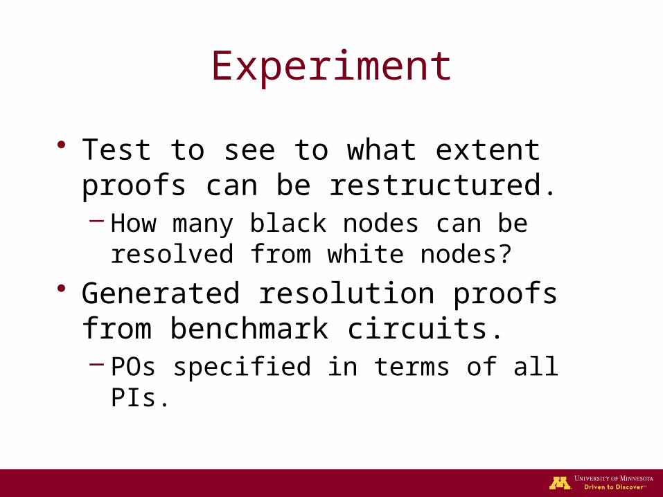
Experiment
• Test to see to what extent proofs can be restructured.– How many black nodes can be resolved
from white nodes?• Generated resolution proofs from
benchmark circuits.– POs specified in terms of all PIs.

BenchmarkOrig. Num.
WhiteOrig. Num.
BlackNum.
CheckedNum.
Sharable%
Sharable Time (s)
dk15 1743 581 581 175 30.12 0.04
5xp1 3203 1636 1636 275 16.81 0.18
sse 3848 2650 2650 563 21.25 0.28
ex6 4055 2731 2731 588 21.53 0.29
s641 6002 5148 5148 2269 44.08 0.46
s510 7851 5092 5092 1155 22.68 0.74
s832 15359 14826 14826 3358 22.65 3.67
planet 40516 43387 43387 10640 24.52 26.39
styr 44079 54128 54128 16578 30.63 33.88
s953 49642 46239 46239 12252 26.5 31.99
bcd 96385 109167 103514 34349 33.18 200
table5 137607 288461 69070 27848 40.32 200
table3 177410 283066 47279 24454 51.72 200

Can effect large structural changes.
Discussion
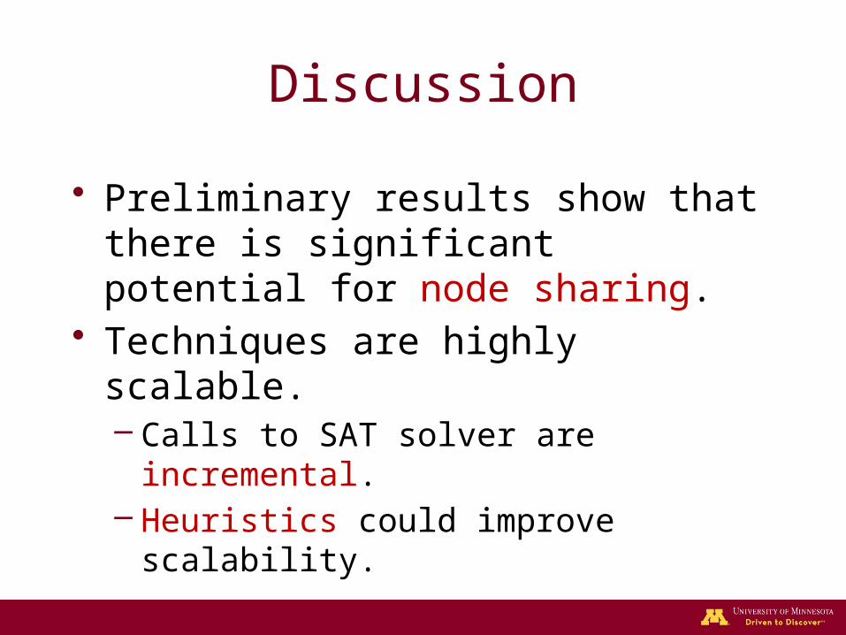
Discussion
• Preliminary results show that there is significant potential for node sharing.
• Techniques are highly scalable.– Calls to SAT solver are incremental.– Heuristics could improve scalability.

How does PDR work?
• The trace contains sets of clauses Fi called frames.
• Frame Fi symbolically represents over approximation of states reachable in i transitions.

Trace Properties
• The 0th frame is initial states ( F0 = I )
• Each frame implies the next ( Fi → Fi+1 )
• Next states are reachable in one transition from current ( Fi ˄ T→ F’
i+1 )
• Every frame satisfies the property; except the last ( Fi → P , i ≠ n)

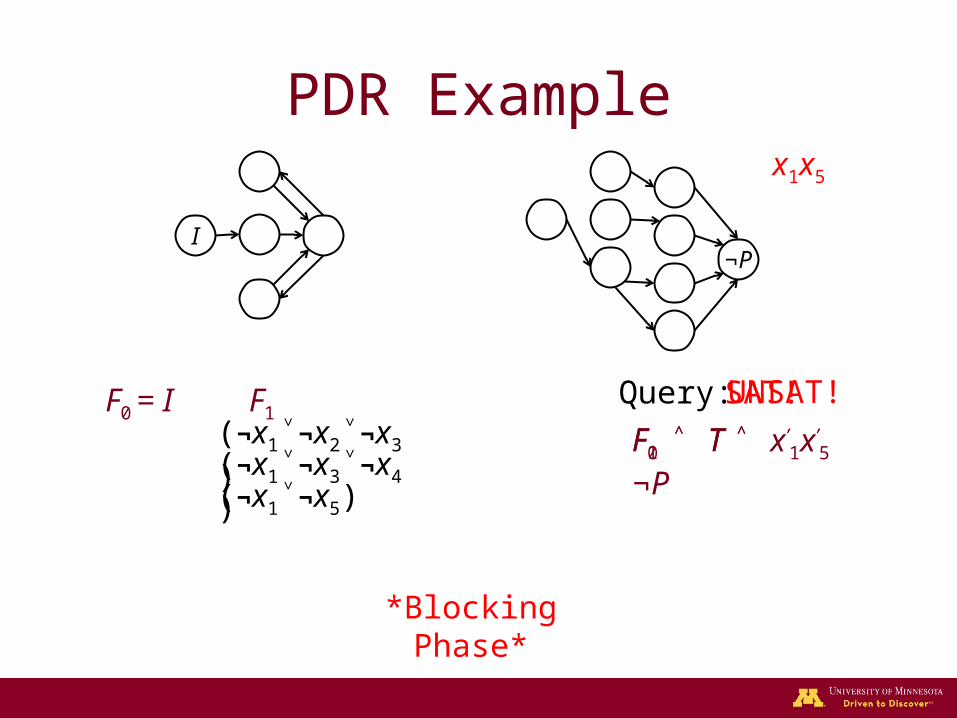
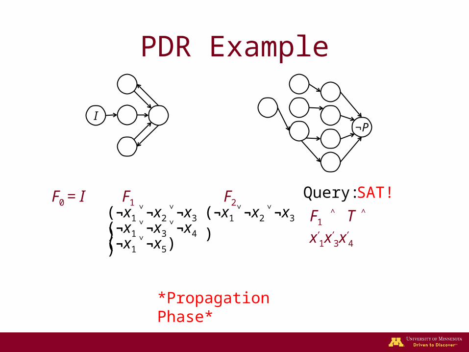
Algorithm Outline
• Consists of two phases:– The blocking phase: determines if cube S
can be blocked in previous time frame i-1 by solving: Fi-1 ˄ T ˄ S’
– The propagation phase: determines if cube S can be blocked in next time frame i+1 by solving: Fi ˄ T ˄ S’

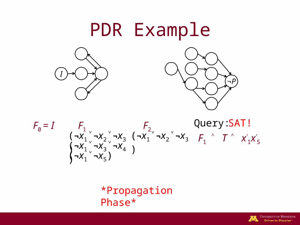
PDR Example
F0 = I F1
F1 ˄ T ˄ ¬P
Query:(¬x1˅¬x2˅¬x3)
¬PI
F0 ˄ T ˄ x’1x’
2x’3x’
4
SAT!UNSAT!
x1x2x3x4
*Blocking Phase*
x4 not in proof!

PDR Example
F0 = I F1
F1 ˄ T ˄ ¬P
Query:
¬PI
F0 ˄ T ˄ x’1x’
3x’4
SAT!UNSAT!(¬x1˅¬x2˅¬x3)(¬x1˅¬x3˅¬x4)
x1x3x4
*Blocking Phase*
PDR Example
F0 = I F1
F1 ˄ T ˄ ¬P
Query:
(¬x1˅¬x5)
¬PI
F0 ˄ T ˄ x’1x’
5
SAT!UNSAT!(¬x1˅¬x2˅¬x3)(¬x1˅¬x3˅¬x4)
x1x5
*Blocking Phase*

PDR Example
F0 = I F1
F1 ˄ T ˄ ¬P
Query:
¬PI
UNSAT!
(¬x1˅¬x5)
(¬x1˅¬x2˅¬x3)(¬x1˅¬x3˅¬x4)
*Blocking Phase*

PDR Example
F0 = I F1Query:
¬PI
F2
F1 ˄ T ˄ x’1x’
2x’3
*Propagation Phase*
UNSAT!
(¬x1˅¬x5)
(¬x1˅¬x2˅¬x3)(¬x1˅¬x3˅¬x4)
(¬x1˅¬x2˅¬x3)
PDR Example
F0 = I F1Query:
¬PI
F2
F1 ˄ T ˄ x’1x’
3x’4
*Propagation Phase*
SAT!
(¬x1˅¬x5)
(¬x1˅¬x2˅¬x3)(¬x1˅¬x3˅¬x4)
(¬x1˅¬x2˅¬x3)
PDR Example
F0 = I F1Query:
¬PI
F2
F1 ˄ T ˄ x’1x’
5
*Propagation Phase*
SAT!
(¬x1˅¬x5)
(¬x1˅¬x2˅¬x3)(¬x1˅¬x3˅¬x4)
(¬x1˅¬x2˅¬x3)

PDR Example
F0 = I F1Query:
¬PI
F2
F2 ˄ T ˄ ¬P
SAT!
(¬x1˅¬x5)
(¬x1˅¬x2˅¬x3)(¬x1˅¬x3˅¬x4)
(¬x1˅¬x2˅¬x3)
x1x3x4
F1 ˄ T ˄ x’1x’
3x’4
x6x7
SAT!
*Blocking Phase*

PDR Example
F0 = I F1Query:
¬PI
F2SAT!
(¬x1˅¬x5)
(¬x1˅¬x2˅¬x3)(¬x1˅¬x3˅¬x4)
(¬x1˅¬x2˅¬x3) F1 ˄ T ˄ x’1x’
3x’4
x6x7x8
F0 ˄ T ˄ x’6x’
7x’8
UNSAT!
(¬x6˅¬x7)
*Blocking Phase*x8 not in proof!

PDR Example
F0 = I F1Query:
¬PI
F2
(¬x1˅¬x5)
(¬x1˅¬x2˅¬x3)(¬x1˅¬x3˅¬x4)
(¬x1˅¬x2˅¬x3) F0 ˄ T ˄ x’6x’
7
UNSAT!
(¬x6˅¬x7)
F1 ˄ T ˄ x’1x’
3x’4(¬x1˅¬x3˅¬x4)
*Blocking Phase*

PDR Example
F0 = I F1Query:
¬PI
F2
(¬x1˅¬x5)
(¬x1˅¬x2˅¬x3)(¬x1˅¬x3˅¬x4)
(¬x1˅¬x2˅¬x3)SAT!
(¬x6˅¬x7)
F2 ˄ T ˄ ¬P(¬x1˅¬x3˅¬x4)
x1x5
F1 ˄ T ˄ x’1x’
5
UNSAT!
(¬x1˅¬x5)
*Blocking Phase*

PDR Example
F0 = I F1Query:
¬PI
F2
(¬x1˅¬x5)
(¬x1˅¬x2˅¬x3)(¬x1˅¬x3˅¬x4)
(¬x1˅¬x2˅¬x3)
(¬x6˅¬x7)
F2 ˄ T ˄ ¬P(¬x1˅¬x3˅¬x4)
UNSAT!
(¬x1˅¬x5)
*Blocking Phase*

PDR Example
F0 = I F1Query:
¬PI
F2
(¬x1˅¬x5)
(¬x1˅¬x2˅¬x3)(¬x1˅¬x3˅¬x4)
(¬x1˅¬x2˅¬x3)
(¬x6˅¬x7)
F1 ˄ T ˄ x’6x’
7(¬x1˅¬x3˅¬x4)(¬x1˅¬x5)
*Propagation Phase*
UNSAT!
(¬x6˅¬x7) F1 = F2 , Fn → P


![What is answer set programming to propositional satisfiability · 1 Introduction Propositional satisfiability (or satisfiability) [6] and answer set programming [7]aretwo closely](https://static.fdocuments.us/doc/165x107/5f0725b47e708231d41b8a72/what-is-answer-set-programming-to-propositional-satisfiability-1-introduction-propositional.jpg)