Algorithmic Complexity Nelson Padua-Perez Bill Pugh Department of Computer Science University of...
41
Algorithmic Complexity Nelson Padua-Perez Bill Pugh Department of Computer Science University of Maryland, College Park
-
date post
19-Dec-2015 -
Category
Documents
-
view
216 -
download
0
Transcript of Algorithmic Complexity Nelson Padua-Perez Bill Pugh Department of Computer Science University of...

Algorithmic Complexity
Nelson Padua-Perez
Bill Pugh
Department of Computer Science
University of Maryland, College Park

Algorithm Efficiency
EfficiencyAmount of resources used by algorithm
Time, space
Measuring efficiencyBenchmarking
Asymptotic analysis

Benchmarking
ApproachPick some desired inputs
Actually run implementation of algorithm
Measure time & space needed
Industry benchmarksSPEC – CPU performance
MySQL – Database applications
WinStone – Windows PC applications
MediaBench – Multimedia applications
Linpack – Numerical scientific applications

Benchmarking
AdvantagesPrecise information for given configuration
Implementation, hardware, inputs
DisadvantagesAffected by configuration
Data sets (usually too small)
Hardware
Software
Affected by special cases (biased inputs)
Does not measure intrinsic efficiency

Asymptotic Analysis
ApproachMathematically analyze efficiency
Calculate time as function of input size n
T O[ f(n) ]
T is on the order of f(n)
“Big O” notation
AdvantagesMeasures intrinsic efficiency
Dominates efficiency for large input sizes

Search Example
Number guessing gamePick a number between 1…n
Guess a number
Answer “correct”, “too high”, “too low”
Repeat guesses until correct number guessed

Linear Search Algorithm
Algorithm1. Guess number = 1
2. If incorrect, increment guess by 1
3. Repeat until correct
ExampleGiven number between 1…100
Pick 20
Guess sequence = 1, 2, 3, 4 … 20
Required 20 guesses
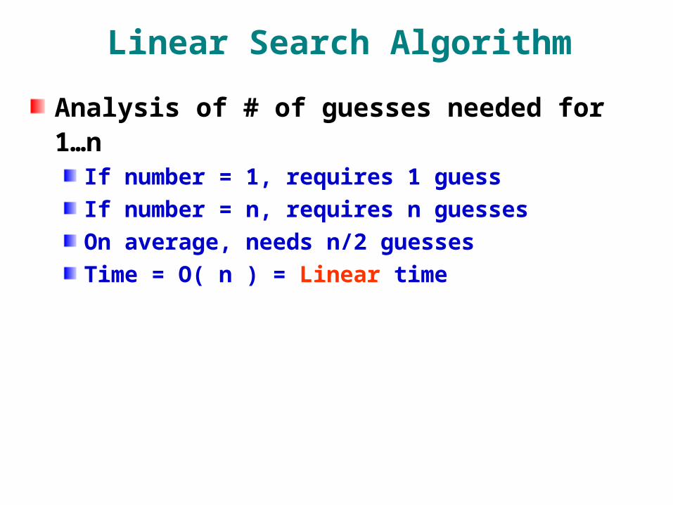
Linear Search Algorithm
Analysis of # of guesses needed for 1…nIf number = 1, requires 1 guess
If number = n, requires n guesses
On average, needs n/2 guesses
Time = O( n ) = Linear time

Binary Search Algorithm
AlgorithmSet to n/4
Guess number = n/2
If too large, guess number – If too small, guess number + Reduce by ½
Repeat until correct

Binary Search Algorithm
ExampleGiven number between 1…100Pick 20Guesses =
50, = 25, Answer = too large, subtract
25, = 12 , Answer = too large, subtract
13, = 6, Answer = too small, add
19, = 3, Answer = too small, add
22, = 1, Answer = too large, subtract
21, = 1, Answer = too large, subtract
20Required 7 guesses

Binary Search Algorithm
Analysis of # of guesses needed for 1…nIf number = n/2, requires 1 guess
If number = 1, requires log2( n ) guesses
If number = n, requires log2( n ) guesses
On average, needs log2( n ) guesses
Time = O( log2( n ) ) = Log time

Search Comparison
For number between 1…100Simple algorithm = 50 steps
Binary search algorithm = log2( n ) = 7 steps
For number between 1…100,000Simple algorithm = 50,000 steps
Binary search algorithm = log2( n ) = 17 steps
Binary search is much more efficient!

Asymptotic Complexity
Comparing two linear functions
Size Running Time
n/2 4n+3
64 32 259
128 64 515
256 128 1027
512 256 2051

Asymptotic Complexity
Comparing two functionsn/2 and 4n+3 behave similarly
Run time roughly doubles as input size doubles
Run time increases linearly with input size
For large values of nTime(2n) / Time(n) approaches exactly 2
Both are O(n) programs
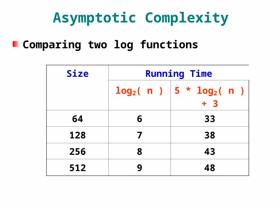
Asymptotic Complexity
Comparing two log functions
Size Running Time
log2( n ) 5 * log2( n ) + 3
64 6 33
128 7 38
256 8 43
512 9 48

Asymptotic Complexity
Comparing two functionslog2( n ) and 5 * log2( n ) + 3 behave similarly
Run time roughly increases by constant as input size doubles
Run time increases logarithmically with input size
For large values of nTime(2n) – Time(n) approaches constant
Base of logarithm does not matter
Simply a multiplicative factorlogaN = (logbN) / (logba)
Both are O( log(n) ) programs

Asymptotic Complexity
Comparing two quadratic functions
Size Running Time
n2 2 n2 + 8
2 4 16
4 16 40
8 64 132
16 256 520

Asymptotic Complexity
Comparing two functionsn2 and 2 n2 + 8 behave similarly
Run time roughly increases by 4 as input size doubles
Run time increases quadratically with input size
For large values of nTime(2n) / Time(n) approaches 4
Both are O( n2 ) programs
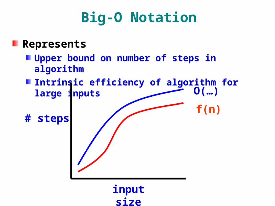
Big-O Notation
RepresentsUpper bound on number of steps in algorithm
Intrinsic efficiency of algorithm for large inputs
f(n)
O(…)
input size
# steps

Formal Definition of Big-O
Function f(n) is ( g(n) ) ifFor some positive constants M, N0
M g(n) f(n), for all n N0
IntuitivelyFor some coefficient M & all data sizes N0
M g(n) is always greater than f(n)
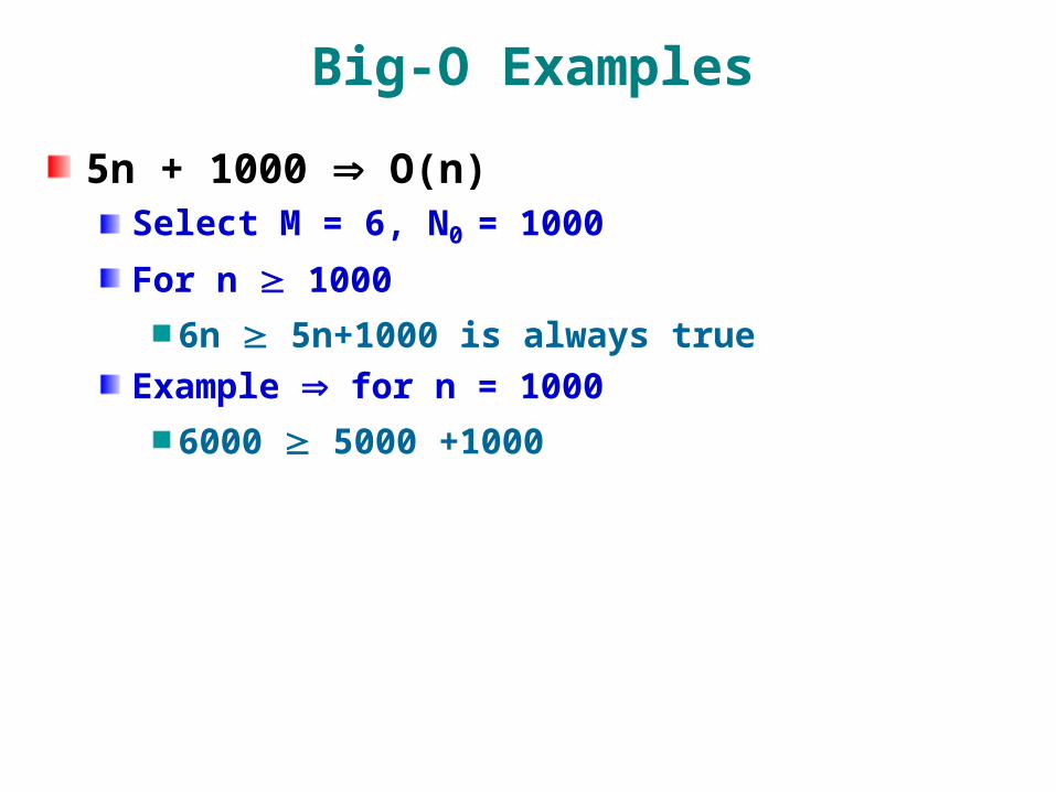
Big-O Examples
5n + 1000 O(n)Select M = 6, N0 = 1000
For n 1000
6n 5n+1000 is always true
Example for n = 1000
6000 5000 +1000

Big-O Examples
2n2 + 10n + 1000 O(n2)Select M = 4, N0 = 100
For n 100
4n2 2n2 + 10n + 1000 is always true
Example for n = 100
40000 20000 + 1000 + 1000

Observations
Big O categoriesO(log(n))
O(n)
O(n2)
For large values of nAny O(log(n)) algorithm is faster than O(n)
Any O(n) algorithm is faster than O(n2)
Asymptotic complexity is fundamental measure of efficiency

Comparison of Complexity

Complexity Category Example
0
50
100
150
200
250
300
1 2 3 4 5 6 7
Problem Size
# of Solution Steps
2^n
n^2
nlog(n)
n
log(n)

Complexity Category Example
1
10
100
1000
1 2 3 4 5 6 7
Problem Size
# of Solution Steps
2^n
n^2
nlog(n)
n
log(n)

Calculating Asymptotic Complexity
As n increasesHighest complexity term dominates
Can ignore lower complexity terms
Examples2 n + 100 O(n)
n log(n) + 10 n O(nlog(n))
½ n2 + 100 n O(n2)
n3 + 100 n2 O(n3)
1/100 2n + 100 n4 O(2n)
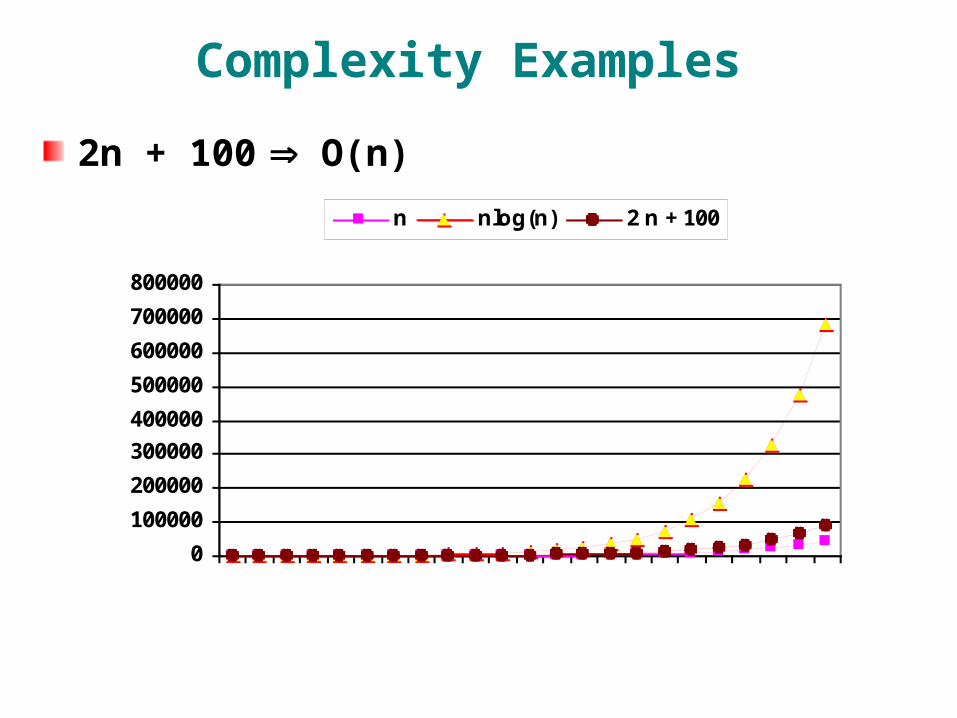
Complexity Examples
2n + 100 O(n)
0
100000
200000
300000
400000
500000
600000
700000
800000
13 49 120 260 533 1068 2118 4175 8208 1611131602
n nlog(n) 2 n + 100

Complexity Examples
½ n log(n) + 10 n O(nlog(n))
0
100000
200000
300000
400000
500000
600000
700000
800000
2 28 79 178 373 756 1506 2975 5855 115012256544252
n nlog(n) 1/2 n log(n) + 10 n

Complexity Examples
½ n2 + 100 n O(n2)
0
100000
200000
300000
400000
500000
600000
700000
800000
2 28 79 178 373 756 1506 2975 5855 115012256544252
nlog(n) n^2 1/2 n^2 + 100 n

Complexity Examples
1/100 2n + 100 n4 O(2n)
11E+151E+301E+451E+601E+751E+90
1E+1051E+1201E+1351E+150
2 13 28 49 79 120 178 260 373 533 756
n^2 n^4 2^n 1 / 100 2^n + 100 n^4

Types of Case Analysis
Can analyze different types (cases) of algorithm behavior
Types of analysisBest case
Worst case
Average case

Types of Case Analysis
Best caseSmallest number of steps required
Not very useful
Example Find item in first place checked
Types of Case Analysis
Worst caseLargest number of steps required
Useful for upper bound on worst performance
Real-time applications (e.g., multimedia)
Quality of service guarantee
Example Find item in last place checked
Quicksort Example
QuicksortOne of the fastest comparison sorts
Frequently used in practice
Quicksort algorithmPick pivot value from list
Partition list into values smaller & bigger than pivot
Recursively sort both lists

Quicksort Example
Quicksort propertiesAverage case = O(nlog(n))
Worst case = O(n2)
Pivot smallest / largest value in list
Picking from front of nearly sorted list
Can avoid worst-case behaviorSelect random pivot value

Types of Case Analysis
Average caseNumber of steps required for “typical” case
Most useful metric in practice
Different approaches
Average case
Expected case
Amortized

Approaches to Average Case
Average caseAverage over all possible inputs
Assumes some probability distribution, usually uniform
Expected caseAlgorithm uses randomness
Worse case over all possible input
average over all possible random values
Amortizedfor all long sequences of operations
worst case total time divided by # of operations

Amortization Example
Adding numbers to end of array of size kIf array is full, allocate new array
Allocation cost is O(size of new array)
Copy over contents of existing array
Two approachesNon-amortized
If array is full, allocate new array of size k+1
Amortized
If array is full, allocate new array of size 2k
Compare their allocation cost

Amortization Example
Non-amortized approachAllocation cost as table grows from 1..n
Total cost n(n+1)/2
Case analysisBest case allocation cost = k
Worse case allocation cost = k
Amortized case allocation cost = (n+1)/2
Size (k) 1 2 3 4 5 6 7 8
Cost 1 2 3 4 5 6 7 8
Amortization Example
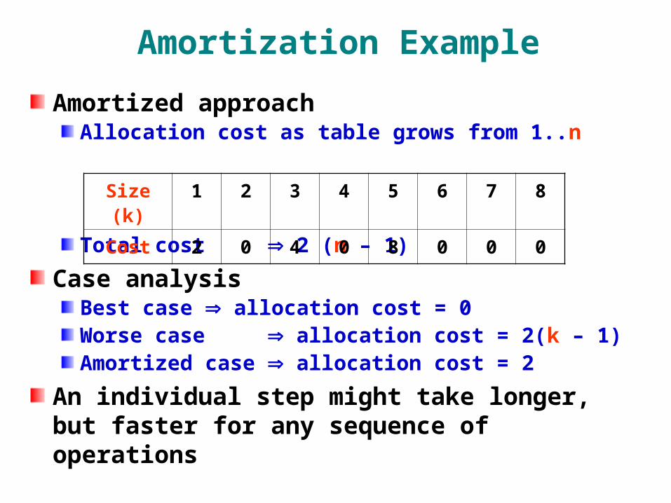
Amortized approachAllocation cost as table grows from 1..n
Total cost 2 (n – 1)
Case analysis Best case allocation cost = 0Worse case allocation cost = 2(k – 1)Amortized case allocation cost = 2
An individual step might take longer, but faster for any sequence of operations
Size (k) 1 2 3 4 5 6 7 8
Cost 2 0 4 0 8 0 0 0