Algorithmic Bayesian Persuasion

Shaddin Dughmi∗

Department of Computer ScienceUniversity of Southern California

shaddin@usc.edu

Haifeng Xu†

Department of Computer ScienceUniversity of Southern California

haifengx@usc.edu

February 14, 2016

Abstract

Persuasion, defined as the act of exploiting an informational advantage in order to effect the decisionsof others, is ubiquitous. Indeed, persuasive communication has been estimated to account for almost athird of all economic activity in the US. This paper examines persuasion through a computational lens,focusing on what is perhaps the most basic and fundamental model in this space: the celebrated Bayesianpersuasion model of Kamenica and Gentzkow [34]. Here there are two players, a sender and a receiver.The receiver must take one of a number of actions with a-priori unknown payoff, and the sender hasaccess to additional information regarding the payoffs of the various actions for both players. The sendercan commit to revealing a noisy signal regarding the realization of the payoffs of various actions, andwould like to do so as to maximize her own payoff in expectation assuming that the receiver rationallyacts to maximize his own payoff. When the payoffs of various actions follow a joint distribution (thecommon prior), the sender’s problem is nontrivial, and its computational complexity depends on therepresentation of this prior.

We examine the sender’s optimization task in three of the most natural input models for this problem,and essentially pin down its computational complexity in each. When the payoff distributions of thedifferent actions are i.i.d. and given explicitly, we exhibit a polynomial-time (exact) algorithmic solution,and a “simple” (1− 1/e)-approximation algorithm. Our optimal scheme for the i.i.d. setting involves ananalogy to auction theory, and makes use of Border’s characterization of the space of reduced-forms forsingle-item auctions. When action payoffs are independent but non-identical with marginal distributionsgiven explicitly, we show that it is #P-hard to compute the optimal expected sender utility. In doing so,we rule out a generalized Border’s theorem, as defined by Gopalan et al [30], for this setting. Finally,we consider a general (possibly correlated) joint distribution of action payoffs presented by a black boxsampling oracle, and exhibit a fully polynomial-time approximation scheme (FPTAS) with a bi-criteriaguarantee. Our FPTAS is based on Monte-Carlo sampling, and its analysis relies on the principle ofdeferred decisions. Moreover, we show that this result is the best possible in the black-box model forinformation-theoretic reasons.

∗Supported in part by NSF CAREER Award CCF-1350900.†Supported by NSF grant CCF-1350900.

1 Introduction“One quarter of the GDP is persuasion.”

This is both the title, and the thesis, of a 1995 paper by McCloskey and Klamer [39]. Since then,persuasion as a share of economic activity appears to be growing — a more recent estimate places the figureat 30% [4]. As both papers make clear, persuasion is intrinsic in most human endeavors. When the tools of“persuasion” are tangible — say goods, services, or money — this is the domain of traditional mechanismdesign, which steers the actions of one or many self-interested agents towards a designer’s objective. What[39, 4] and much of the relevant literature refer to as persuasion, however, are scenarios in which the powerto persuade derives from an informational advantage of some party over others. This is also the sensein which we use the term. Such scenarios are increasingly common in the information economy, and it istherefore unsurprising that persuasion has been the subject of a large body of work in recent years, motivatedby domains as varied as auctions [9, 25, 24, 10], advertising [3, 33, 17], voting [2], security [46, 42], multi-armed bandits [37, 38], medical research [35], and financial regulation [28, 29]. (For an empirical surveyof persuasion, we refer the reader to [21]). What is surprising, however, is the lack of systematic study ofpersuasion through a computational lens; this is what we embark on in this paper.

In the large body of literature devoted to persuasion, perhaps no model is more basic and fundamentalthan the Bayesian Persuasion model of Kamenica and Gentzkow [34], generalizing an earlier model byBrocas and Carrillo [14]. Here there are two players, who we call the sender and the receiver. The receiveris faced with selecting one of a number of actions, each of which is associated with an a-priori unknownpayoff to both players. The state of nature, describing the payoff to the sender and receiver from each action,is drawn from a prior distribution known to both players. However, the sender possesses an informationaladvantage, namely access to the realized state of nature prior to the receiver choosing his action. In order topersuade the receiver to take a more favorable action for her, the sender can commit to a policy, often knownas an information structure or signaling scheme, of releasing information about the realized state of nature tothe receiver before the receiver makes his choice. This policy may be simple, say by always announcing thepayoffs of the various actions or always saying nothing, or it may be intricate, involving partial informationand added noise. Crucially, the receiver is aware of the sender’s committed policy, and moreover is rationaland Bayesian. We examine the sender’s algorithmic problem of implementing the optimal signaling schemein this paper. A solution to this problem, i.e., a signaling scheme, is an algorithm which takes as input thedescription of a state of nature and outputs a signal, potentially utilizing some internal randomness.

1.1 Two ExamplesTo illustrate the intricacy of Bayesian Persuasion, Kamenica and Gentzkow [34] use a simple example inwhich the sender is a prosecutor, the receiver is a judge, and the state of nature is the guilt or innocenceof a defendant. The receiver (judge) has two actions, conviction and acquittal, and wishes to maximizethe probability of rendering the correct verdict. On the other hand, the sender (prosecutor) is interestedin maximizing the probability of conviction. As they show, it is easy to construct examples in which theoptimal signaling scheme for the sender releases noisy partial information regarding the guilt or innocenceof the defendant. For example, if the defendant is guilty with probability 1

3 , the prosecutor’s best strategyis to claim “guilt” whenever the defendant is guilty, and also claim “guilt” just under half the time whenthe defendant is innocent. As a result, the defendant will be convicted whenever the prosecutor claims“guilt” (happening with probability just under 2

3 ), assuming that the judge is fully aware of the prosecutor’ssignaling scheme. We note that it is not in the prosecutor’s interest to always claim “guilt”, since a rationaljudge aware of such a policy would ascribe no meaning to such a signal, and render his verdict based solelyon his prior belief — in this case, this would always lead to acquittal.1

1In other words, a signal is an abstract object with no intrinsic meaning, and is only imbued with meaning by virtue of how it isused. In particular, a signal has no meaning beyond the posterior distribution on states of nature it induces.

1

A somewhat less artificial example of persuasion is in the context of providing financial advice. Here,the receiver is an investor, actions correspond to stocks, and the sender is a stockbroker or financial adviserwith access to stock return projections which are a-priori unknown to the investor. When the adviser’scommission or return is not aligned with the investor’s returns, this is a nontrivial Bayesian persuasionproblem. In fact, interesting examples exist when stock returns are independent from each other, or eveni.i.d. Consider the following simple example which fits into the i.i.d. model considered in Section 3: thereare two stocks, each of which is a-priori equally likely to generate low (L), moderate (M), or high (H)short-term returns to the investor (independently). We refer to L/M/H as the types of a stock, and associatethem with short-term returns of 0, 1 + ε, and 2 respectively. Suppose, also, that stocks of type L or H areassociated with poor long-term returns of 0; in the case of H, high short-term returns might be an indicationof volatility or overvaluation, and hence poor long-term performance. This leaves stocks of type M as theonly solid performers with long-term returns of 1. Now suppose that the investor is myopically interested inmaximizing short-term returns, whereas the forward-looking financial adviser is concerned with maximizinglong-term returns, perhaps due to reputational considerations. Simple calculation shows that providing fullinformation to the myopic investor results in an expected long-term reward of 1

3 , as does providing noinformation. An optimal signaling scheme, which guarantees that the investor chooses a stock with typeM whenever such a stock exists, is the following: when exactly one of the stocks has type M recommendthat stock, and otherwise recommend a stock uniformly at random. A simple calculation using Bayes’ ruleshows that the investor prefers to follow the recommendations of this partially-informative scheme, and itfollows that the expected long-term return is 5

9 .

1.2 Results and TechniquesMotivated by these intricacies, we study the computational complexity of optimal and near-optimal persua-sion in the presence of multiple actions. We first observe that a linear program with a variable for each(state-of-nature, action) pair computes a description of the optimal signaling scheme. However, when ac-tion payoffs are distributed according to a joint distribution — say exhibiting some degree of independenceacross different actions — the number of states of nature may be exponential in the number of actions; insuch settings, both the number of variables and constraints of this linear program are exponential in thenumber of actions. It is therefore unsurprising that the computational complexity of persuasion dependson how the prior distribution on states of nature is presented as input. We therefore consider three naturalinput models in increasing order of generality, and mostly pin down the complexity of optimal and near-optimal persuasion in each. Our first model assumes that action payoffs are drawn i.i.d. from an explicitlydescribed marginal distribution. Our second model considers independent yet non-identical actions, againwith explicitly-described marginals. Our third and most general model considers an arbitrary joint distribu-tion of action payoffs presented by a black-box sampling oracle. In proving our results, we draw connectionsto techniques and concepts developed in the context of Bayesian mechanism design (BMD), exercising andgeneralizing them along the way as needed to prove our results. We mention some of these connectionsbriefly here, and elaborate on the similarities and differences from the BMD literature in Appendix A.

We start with the i.i.d model, and show two results: a “simple” and polynomial-time e−1e -approximate

signaling scheme, and a polynomial-time implementation of the optimal scheme. Both results hinge on a“symmetry characterization” of the optimal scheme in the i.i.d. setting, closely related to the symmetrizationresult from BMD by [20] but with an important difference which we discuss in Appendix A. Our “simple”scheme decouples the signaling problem for the different actions and signals independently for each. Thisresult implies that signaling in this setting can be “distributed” among multiple non-coordinating persuaderswithout much loss. Our optimal scheme involves a connection to Border’s characterization of the spaceof feasible reduced-form auctions [13, 12], as well as its algorithmic properties [15, 1]. This connectioninvolves proving a correspondence between “symmetric” signaling schemes and a subset of “symmetric”single-item auctions; one in which actions in persuasion correspond to bidders in an auction.

2

Next, we consider Bayesian persuasion with independent non-identical actions. One might expect thatthe partial correspondence between signaling schemes and single-item auctions in the i.i.d. model gen-eralizes here, in which case Border’s theorem — which extends to single-item auctions with independentnon-identical bidders — would analogously lead to polynomial time algorithm for persuasion in this setting.However, we surprisingly show that this analogy to single-item auctions ceases to hold for non-identicalactions: we prove that there is no generalized Border’s theorem, in the sense of Gopalan et al. [30], for per-suasion with independent actions. Specifically, we show that it is #P-hard to exactly compute the expectedsender utility for the optimal scheme, ruling out Border’s-theorem-like approaches to this problem unlessthe polynomial hierarchy collapses. Our proof starts from the ideas of [30], but our reduction is much moreinvolved and goes through the membership problem for an implicit polytope which encodes a #P-hard prob-lem — we elaborate on these differences in Appendix A. We note that whereas we do rule out computing anexplicit representation of the optimal scheme which permits evaluating optimal sender utility, we do not ruleout other approaches which might sample the optimal scheme “on the fly” in the style of Myerson’s optimalauction [41]— we leave the intriguing question of whether this is possible as an open problem.

Finally, we consider the black-box model with general distributions, and prove essentially-matching pos-itive and negative results. For our positive result, we exhibit fully polynomial-time approximation scheme(FPTAS) with a bicriteria guarantee. Specifically, our scheme loses an additive ε in both expected senderutility and incentive-compatibility (as defined in Section 2), and runs in time polynomial in the number ofactions and 1

ε . Our negative results show that this is essentially the best possible for information-theoreticreasons: any polynomial-time scheme in the black box model which comes close to optimality must signif-icantly sacrifice incentive compatibility, and vice versa. We note that our scheme is related to some priorwork on BMD with black-box distributions [16, 45], but is significantly simpler and more efficient: insteadof using the ellipsoid method to optimize over “reduced forms”, our scheme simply solves a single linearprogram on a sample from the prior distribution on states of nature. Such simplicity is possible in our settingdue to the different notion of incentive compatibility in persuasion, which reduces to incentive compatibilityon the sample using the principle of deferred decisions. We elaborate on this connection in Appendix A.

We remark that our results suggest that the differences between persuasion and auction design serve asa double-edged sword. This is evidenced by our negative result for independent model and our “simple”positive result for the black-box model.

1.3 Additional Discussion of Related WorkTo our knowledge, Brocas and Carrillo [14] were the first to explicitly consider persuasion through informa-tion control. They consider a sender with the ability to costlessly acquire information regarding the payoffsof the receiver’s actions, with the stipulation that acquired information is available to both players. Thisis technically equivalent to our (and Kamenica and Gentzkow’s [34]) informed sender who commits to asignaling scheme. Brocas and Carrillo restrict attention to a particular setting with two states of nature andthree actions, and characterize optimal policies for the sender and their associated payoffs. Kamenica andGentzkow’s [34] Bayesian Persuasion model naturally generalizes [14] to finite (or infinite yet compact)states of nature and action spaces. They establish a number of properties of optimal information structuresin this model; most notably, they characterize settings in which signaling strictly benefits the sender in termsof the convexity/concavity of the sender’s payoff as a function of the receiver’s posterior belief.

Since [14] and [34], an explosion of interest in persuasion problems followed. The basic Bayesianpersuasion model underlies, or is closely related to, recent work in a number of different domains: pricediscrimination by Bergemann et al. [10], advertising by Chakraborty and Harbaugh [17], security gamesby Xu et al. [46] and Rabinovich et al. [42], multi-armed bandits by Kremer et al. [37] and Mansour et al.[38], medical research by Kolotilin [35], and financial regulation by Gick and Pausch [28] and Goldsteinand Leitner [29]. Generalizations and variants of the Bayesian persuasion model have also been considered:Gentzkow and Kamenica [26] consider multiple senders, Alonso and Camara [2] consider multiple receivers

3

in a voting setting, Gentzkow and Kamenica [27] consider costly information acquisition, Rayo and Segal[43] consider an outside option for the receiver, and Kolotilin et al. [36] considers a receiver with privateside information.

Optimal persuasion is a special case of information structure design in games, also known as signal-ing. The space of information structures, and their induced equilibria, are characterized by Bergemann andMorris [8]. Recent work in the CS community has also examined the design of information structures algo-rithmically. Work by Emek et al. [24], Miltersen and Sheffet [40], Guo and Deligkas [32], and Dughmi et al.[23], examine optimal signaling in a variety of auction settings, and presents polynomial-time algorithmsand hardness results. Dughmi [22] exhibits hardness results for signaling in two-player zero-sum games, andCheng et al. [18] present an algorithmic framework and apply it to a number of different signaling problems.

Also related to the Bayesian persuasion model is the extensive literature on cheap talk starting withCrawford and Sobel [19]. Cheap talk can be viewed as the analogue of persuasion when the sender cannotcommit to an information revelation policy. Nevertheless, the commitment assumption in persuasion hasbeen justified on the grounds that it arises organically in repeated cheap talk interactions with a long horizon— in particular when the sender must balance his short term payoffs with long-term credibility. We referthe reader to the discussion of this phenomenon in [43]. Also to this point, Kamenica and Gentzkow [34]mention that an earlier model of repeated 2-player games with asymmetric information by Aumann andMaschler [5] is mathematically analogous to Bayesian persuasion.

Various recent models on selling information in [6, 7, 11] are quite similar to Bayesian persuasion, withthe main difference being that the sender’s utility function is replaced with revenue. Whereas Babaioff et al.[6] consider the algorithmic question of selling information when states of nature are explicitly given asinput, the analogous algorithmic questions to ours have not been considered in their model. We speculatethat some of our algorithmic techniques might be applicable to models for selling information when theprior distribution on states of nature is represented succinctly.

As discussed previously, our results involve exercising and generalizing ideas from prior work in Bayesianmechanism design. We view drawing these connections as one of the contributions of our paper. In Ap-pendix A, we discuss these connections and differences at length.

2 PreliminariesIn a persuasion game, there are two players: a sender and a receiver. The receiver is faced with selectingan action from [n] = 1, . . . , n, with an a-priori-unknown payoff to each of the sender and receiver. Weassume payoffs are a function of an unknown state of nature θ, drawn from an abstract set Θ of potentialrealizations of nature. Specifically, the sender and receiver’s payoffs are functions s, r : Θ × [n] → R,respectively. We use r = r(θ) ∈ Rn to denote the receiver’s payoff vector as a function of the stateof nature, where ri(θ) is the receiver’s payoff if he takes action i and the state of nature is θ. Similarlys = s(θ) ∈ Rn denotes the sender’s payoff vector, and si(θ) is the sender’s payoff if the receiver takesaction i and the state is θ. Without loss of generality, we often conflate the abstract set Θ indexing states ofnature with the set of realizable payoff vector pairs (s, r) — i.e., we think of Θ as a subset of Rn ×Rn. Weassume that Θ is finite for notational convenience, though this is not needed for our results in Section 5.

In Bayesian persuasion, it is assumed that the state of nature is a-priori unknown to the receiver, anddrawn from a common-knowledge prior distribution λ supported on Θ. The sender, on the other hand, hasaccess to the realization of θ, and can commit to a policy of partially revealing information regarding itsrealization before the receiver selects his action. Specifically, the sender commits to a signaling scheme ϕ,mapping (possibly randomly) states of nature Θ to a family of signals Σ. For θ ∈ Θ, we use ϕ(θ) to denotethe (possibly random) signal selected when the state of nature is θ. Moreover, we use ϕ(θ, σ) to denote theprobability of selecting the signal σ given a state of nature θ. An algorithm implements a signaling schemeϕ if it takes as input a state of nature θ, and samples the random variable ϕ(θ).

Given a signaling scheme ϕ with signals Σ, each signal σ ∈ Σ is realized with probability ασ =

4

∑θ∈Θ λθϕ(θ, σ). Conditioned on the signal σ, the expected payoffs to the receiver of the various actions

are summarized by the vector r(σ) = 1ασ

∑θ∈Θ λθϕ(θ, σ)r(θ). Similarly, the sender’s payoff as a function

of the receiver’s action are summarized by s(σ) = 1ασ

∑θ∈Θ λθϕ(θ, σ)s(θ). On receiving a signal σ, the

receiver performs a Bayesian update and selects an action i∗(σ) ∈ argmaxi ri(σ) with expected receiverutility maxi ri(σ). This induces utility si∗(σ)(σ) for the sender. In the event of ties when selecting i∗(σ),we assume those ties are broken in favor of the sender.

We adopt the perspective of a sender looking to designϕ to maximize her expected utility∑

σ ασsi∗(σ)(σ),in which case we say ϕ is optimal. When ϕ yields expected sender utility within an additive [multiplicative]ε of the best possible, we say it is ε-optimal [ε-approximate] in the additive [multiplicative] sense. A simplerevelation-principle style argument [34] shows that an optimal signaling scheme need not use more than nsignals, with one recommending each action. Such a direct scheme ϕ has signals Σ = σ1, . . . , σn, andsatisfies ri(σi) ≥ rj(σi) for all i, j ∈ [n]. We think of σi as a signal recommending action i, and the require-ment ri(σi) ≥ maxj rj(σi) as an incentive-compatibility (IC) constraint on our signaling scheme. We cannow write the sender’s optimization problem as the following LP with variables ϕ(θ, σi) : θ ∈ Θ, i ∈ [n].

maximize∑

θ∈Θ

∑ni=1 λθϕ(θ, σi)si(θ)

subject to∑n

i=1 ϕ(θ, σi) = 1, for θ ∈ Θ.∑θ∈Θ λθϕ(θ, σi)ri(θ) ≥

∑θ∈Θ λθϕ(θ, σi)rj(θ), for i, j ∈ [n].

ϕ(θ, σi) ≥ 0, for θ ∈ Θ, i ∈ [n].

(1)

For our results in Section 5, we relax our incentive constraints by assuming that the receiver follows therecommendation so long as it approximately maximizes his utility — for a parameter ε > 0, we relax our re-quirement to ri(σi) ≥ maxj rj(σi)−ε, which translates to the relaxed IC constraints

∑θ∈Θ λθϕ(θ, σi)ri(θ) ≥∑

θ∈Θ λθϕ(θ, σi)(rj(θ) − ε) in LP (1). We call such schemes ε-incentive compatible (ε-IC). We judge thesuboptimality of an ε-IC scheme relative to the best (absolutely) IC scheme; i.e., in a bi-criteria sense.

Finally, we note that expected utilities, incentive compatibility, and optimality are properties not onlyof a signaling scheme ϕ, but also of the distribution λ over its inputs. When λ is not clear from contextand ϕ is supported on a superset of λ, we often say that a signaling scheme ϕ is IC [ε-IC] for λ, or optimal[ε-optimal] for λ. We also use us(ϕ, λ) to denote the expected sender utility

∑θ∈Θ

∑ni=1 λθϕ(θ, σi)si(θ).

3 Persuasion with I.I.D. ActionsIn this section, we assume the payoffs of different actions are independently and identically distributed (i.i.d.)according to an explicitly-described marginal distribution. Specifically, each state of nature θ is a vector inΘ = [m]n for a parameter m, where θi ∈ [m] is the type of action i. Associated with each type j ∈ [m] isa pair (ξj , ρj) ∈ R2, where ξj [ρj] is the payoff to the sender [receiver] when the receiver chooses an actionwith type j. We are given a marginal distribution over types, described by a vector q = (q1, ..., qm) ∈ ∆m.We assume each action’s type is drawn independently according to q; specifically, the prior distribution λon states of nature is given by λ(θ) =

∏i∈[n] qθi . For convenience, we let ξ = (ξ1, ..., ξm) ∈ Rm and

ρ = (ρ1, ..., ρm) ∈ Rm denote the type-indexed vectors of sender and receiver payoffs, respectively. Weassume ξ, ρ, and q — the parameters describing an i.i.d. persuasion instance — are given explicitly.

Note that the number of states of nature is mn, and therefore the natural representation of a signalingscheme has nmn variables. Moreover, the natural linear program for the persuasion problem in Section 2has an exponential in n number of both variables and constraints. Nevertheless, as mentioned in Section 2we seek only to implement an optimal or near-optimal scheme ϕ as an oracle which takes as input θ andsamples a signal σ ∼ ϕ(θ). Our algorithms will run in time polynomial in n and m, and will optimize overa space of succinct “reduced forms” for signaling schemes which we term signatures, to be described next.

For a state of nature θ, define the matrixM θ ∈ 0, 1n×m so thatM θij = 1 if and only if action i has type

j in θ (i.e. θi = j). Given an i.i.d prior λ and a signaling scheme ϕ with signals Σ = σ1, . . . , σn, for each

5

Mσi =∑

θ λ(θ)ϕ(θ, σi)Mθ, for i = 1, . . . , n.∑n

i=1 ϕ(θ, σi) = 1, for θ ∈ Θ.ϕ(θ, σi) ≥ 0, for θ ∈ Θ, i ∈ [n].

Figure 1: Realizable Signatures P

max∑n

i=1 ξ ·Mσii

s.t. ρ ·Mσii ≥ ρ ·M

σij , for i, j ∈ [n].

(Mσ1 , ...,Mσn) ∈ P

Figure 2: Persuasion in Signature Space

i ∈ [n] let αi =∑

θ λ(θ)ϕ(θ, σi) denote the probability of sending σi, and let Mσi =∑

θ λ(θ)ϕ(θ, σi)Mθ.

Note thatMσijk is the joint probability that action j has type k and the scheme outputs σi. Also note that each

row of Mσi sums to αi, and the jth row represents the un-normalized posterior type distribution of action jgiven signal σi. We callM = (Mσ1 , ...,Mσn) ∈ Rn×m×n the signature of ϕ. The sender’s objective andreceiver’s IC constraints can both be expressed in terms of the signature. In particular, using Mj to denotethe jth row of a matrix M , the IC constraints are ρ ·Mσi

i ≥ ρ ·Mσij for all i, j ∈ [n], and the sender’s

expected utility assuming the receiver follows the scheme’s recommendations is∑

i∈[n] ξ ·Mσii .

We sayM = (Mσ1 , ...,Mσn) ∈ Rn×m×n is realizable if there exists a signaling scheme ϕ withM asits signature. Realizable signatures constitutes a polytope P ⊆ Rn×m×n, which has an exponential-sizedextended formulation as shown Figure 1. Given this characterization, the sender’s optimization problem canbe written as a linear program in the space of signatures, shown in Figure 2:

3.1 Symmetry of the Optimal Signaling SchemeWe now show that there always exists a “symmetric” optimal scheme when actions are i.i.d. Given a signa-tureM = (Mσ1 , ...,Mσn), it will sometimes be convenient to think of it as the set of pairs (Mσi , σi)i∈[n].

Definition 3.1. A signaling scheme ϕ with signature (Mσi , σi)i∈[n] is symmetric if there exist x,y ∈ Rmsuch that Mσi

i = x for all i ∈ [n] and Mσij = y for all j 6= i. The pair (x,y) is the s-signature of ϕ.

In other words, a symmetric signaling scheme sends each signal with equal probability ||x||1, and in-duces only two different posterior type distributions for actions: x

||x||1 for the recommended action, and y||y||1

for the others. We call (x,y) realizable if there exists a signaling scheme with (x,y) as its s-signature. Thefamily of realizable s-signatures constitutes a polytope Ps, and has an extended formulation by adding thevariables x,y ∈ Rm and constraints Mσi

i = x and Mσij = y for all i, j ∈ [n] with i 6= j to the extended

formulation of (asymmetric) realizable signatures from Figure 1.We make two simple observations regarding realizable s-signatures. First, ||x||1 = ||y||1 = 1

n foreach (x,y) ∈ Ps, and this is because both ||x||1 and ||y||1 equal the probability of each of the n signals.Second, since the signature must be consistent with prior marginal distribution q, we have x+ (n− 1)y =∑n

i=1Mσi1 = q. We show that restricting to symmetric signaling schemes is without loss of generality.

Theorem 3.2. When the action payoffs are i.i.d., there exists an optimal and incentive-compatible signalingscheme which is symmetric.

Theorem 3.2 is proved in Appendix B.1. At a high level, we show that optimal signaling schemes areclosed with respect to two operations: convex combination and permutation. Specifically, a convex combi-nation of realizable signatures — viewed as vectors in Rn×m×n — is realized by the corresponding “randommixture” of signaling schemes, and this operation preserves optimality. The proof of this fact follows easilyfrom the fact that linear program in Figure 2 has a convex family of optimal solutions. Moreover, given apermutation π ∈ Sn and an optimal signatureM = (Mσi , σi)i∈[n] realized by signaling scheme ϕ, the“permuted” signature π(M) = (πMσi , σπ(i))i∈[n] — where premultiplication of a matrix by π denotespermuting the rows of the matrix — is realized by the “permuted” scheme ϕπ(θ) = π(ϕ(π−1(θ))), whichis also optimal. The proof of this fact follows from the “symmetry” of the (i.i.d.) prior distribution about thedifferent actions. Theorem 3.2 is then proved constructively as follows: given a realizable optimal signatureM, the “symmetrized” signatureM = 1

n!

∑π∈Sn π(M) is realizable, optimal, and symmetric.

6

3.2 Implementing the Optimal Signaling SchemeWe now exhibit a polynomial-time algorithm for persuasion in the i.i.d. model. Theorem 3.2 permits re-writing the optimization problem in Figure 2 as follows, with variables x,y ∈ Rm.

maximize nξ · xsubject to ρ · x ≥ ρ · y

(x,y) ∈ Ps(2)

Problem (2) cannot be solved directly, since Ps is defined by an extended formulation with exponentiallymany variables and constraints, as described in Section 3.1. Nevertheless, we make use of a connectionbetween symmetric signaling schemes and single-item auctions with i.i.d. bidders to solve (2) using theEllipsoid method. Specifically, we show a one-to-one correspondence between symmetric signatures and (asubset of) symmetric reduced forms of single-item auctions with i.i.d. bidders, defined as follows.

Definition 3.3 ([13]). Consider a single-item auction setting with n i.i.d. bidders and m types for eachbidder, where each bidder’s type is distributed according to q ∈ ∆m. An allocation rule is a randomizedfunction A mapping a type profile θ ∈ [m]n to a winner A(θ) ∈ [n] ∪ ∗, where ∗ denotes not allocatingthe item. We say the allocation rule has symmetric reduced form τ ∈ [0, 1]m if for each bidder i ∈ [n] andtype j ∈ [m], τj is the conditional probability of i receiving the item given she has type j.

When q is clear from context, we say τ is realizable if there exists an allocation rule with τ as its symmetricreduced form. We say an algorithm implements an allocation rule A if it takes as input θ, and samples A(θ).

Theorem 3.4. Consider the Bayesian Persuasion problem with n i.i.d. actions andm types, with parametersq ∈ ∆m, ξ ∈ Rm, and ρ ∈ Rm given explicitly. An optimal and incentive-compatible signaling scheme canbe implemented in poly(m,n) time.

Theorem 3.4 is a consequence of the following set of lemmas.

Lemma 3.5. Let (x,y) ∈ [0, 1]m × [0, 1]m, and define τ = (x1q1 , ...,xmqm

). The pair (x,y) is a realizables-signature if and only if (a) ||x||1 = 1

n , (b) x+ (n− 1)y = q, and (c) τ is a realizable symmetric reducedform of an allocation rule with n i.i.d. bidders, m types, and type distribution q. Moreover, assuming x andy satisfy (a), (b) and (c), and given black-box access to an allocation rule A with symmetric reduced formτ , a signaling scheme with s-signature (x,y) can be implemented in poly(n,m) time.

Lemma 3.6. An optimal realizable s-signature, as described by LP (2), is computable in poly(n,m) time.

Lemma 3.7. (See [15, 1]) Consider a single-item auction setting with n i.i.d. bidders and m types for eachbidder, where each bidder’s type is distributed according to q ∈ ∆m. Given a realizable symmetric reducedform τ ∈ [0, 1]m, an allocation rule with reduced form τ can be implemented in poly(n,m) time.

The proofs of Lemmas 3.5 and 3.6 can be found in Appendix B.2. The proof of Lemma 3.5 buildsa correspondence between s-signatures of signaling schemes and certain reduced-form allocation rules.Specifically, actions correspond to bidders, action types correspond to bidder types, and signaling σi cor-responds to assigning the item to bidder i. The expression of the reduced form in terms of the s-signaturethen follows from Bayes’ rule. Lemma 3.6 follows from Lemma 3.5, the ellipsoid method, and the fact thatsymmetric reduced forms admit an efficient separation oracle (see [13, 12, 15, 1]).

7

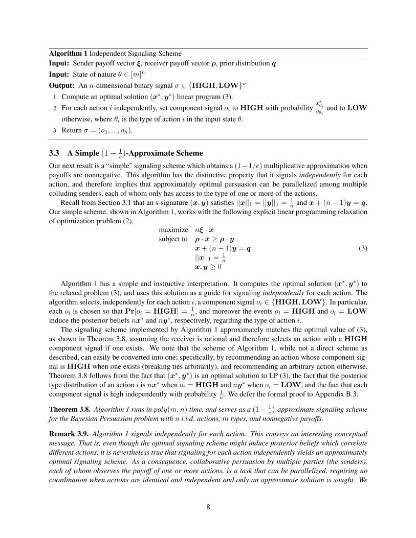
Algorithm 1 Independent Signaling SchemeInput: Sender payoff vector ξ, receiver payoff vector ρ, prior distribution q

Input: State of nature θ ∈ [m]n

Output: An n-dimensional binary signal σ ∈ HIGH,LOWn

1: Compute an optimal solution (x∗,y∗) linear program (3).

2: For each action i independently, set component signal oi to HIGH with probabilityx∗θiqθi

and to LOW

otherwise, where θi is the type of action i in the input state θ.

3: Return σ = (o1, ..., on).

3.3 A Simple (1− 1e)-Approximate Scheme

Our next result is a “simple” signaling scheme which obtains a (1−1/e) multiplicative approximation whenpayoffs are nonnegative. This algorithm has the distinctive property that it signals independently for eachaction, and therefore implies that approximately optimal persuasion can be parallelized among multiplecolluding senders, each of whom only has access to the type of one or more of the actions.

Recall from Section 3.1 that an s-signature (x,y) satisfies ||x||1 = ||y||1 = 1n and x + (n − 1)y = q.

Our simple scheme, shown in Algorithm 1, works with the following explicit linear programming relaxationof optimization problem (2).

maximize nξ · xsubject to ρ · x ≥ ρ · y

x+ (n− 1)y = q||x||1 = 1

nx,y ≥ 0

(3)

Algorithm 1 has a simple and instructive interpretation. It computes the optimal solution (x∗,y∗) tothe relaxed problem (3), and uses this solution as a guide for signaling independently for each action. Thealgorithm selects, independently for each action i, a component signal oi ∈ HIGH,LOW. In particular,each oi is chosen so that Pr[oi = HIGH] = 1

n , and moreover the events oi = HIGH and oi = LOWinduce the posterior beliefs nx∗ and ny∗, respectively, regarding the type of action i.

The signaling scheme implemented by Algorithm 1 approximately matches the optimal value of (3),as shown in Theorem 3.8, assuming the receiver is rational and therefore selects an action with a HIGHcomponent signal if one exists. We note that the scheme of Algorithm 1, while not a direct scheme asdescribed, can easily be converted into one; specifically, by recommending an action whose component sig-nal is HIGH when one exists (breaking ties arbitrarily), and recommending an arbitrary action otherwise.Theorem 3.8 follows from the fact that (x∗,y∗) is an optimal solution to LP (3), the fact that the posteriortype distribution of an action i is nx∗ when oi = HIGH and ny∗ when oi = LOW, and the fact that eachcomponent signal is high independently with probability 1

n . We defer the formal proof to Appendix B.3.

Theorem 3.8. Algorithm 1 runs in poly(m,n) time, and serves as a (1− 1e )-approximate signaling scheme

for the Bayesian Persuasion problem with n i.i.d. actions, m types, and nonnegative payoffs.

Remark 3.9. Algorithm 1 signals independently for each action. This conveys an interesting conceptualmessage. That is, even though the optimal signaling scheme might induce posterior beliefs which correlatedifferent actions, it is nevertheless true that signaling for each action independently yields an approximatelyoptimal signaling scheme. As a consequence, collaborative persuasion by multiple parties (the senders),each of whom observes the payoff of one or more actions, is a task that can be parallelized, requiring nocoordination when actions are identical and independent and only an approximate solution is sought. We

8

leave open the question of whether this is possible when action payoffs are independently but not identicallydistributed.

4 Complexity Barriers to Persuasion with Independent ActionsIn this section, we consider optimal persuasion with independent action payoffs as in Section 3, albeitwith action-specific marginal distributions given explicitly. Specifically, for each action i we are givena distribution qi ∈ ∆mi on mi types, and each type j ∈ [mi] of action i is associated with a senderpayoff ξij ∈ R and a receiver payoff ρij ∈ R. The positive results of Section 3 draw a connection betweenoptimal persuasion in the special case of identically distributed actions and Border’s characterization ofreduced-form single-item auctions with i.i.d. bidders. One might expect this connection to generalize to theindependent non-identical persuasion setting, since Border’s theorem extends to single-item auctions withindependent non-identical bidders. Surprisingly, we show that this analogy to Border’s characterization failsto generalize. We prove the following theorem.

Theorem 4.1. Consider the Bayesian Persuasion problem with independent actions, with action-specificpayoff distributions given explicitly. It is #P -hard to compute the optimal expected sender utility.

Invoking the framework of Gopalan et al. [30], this rules out a generalized Border’s theorem for oursetting, in the sense defined by [30], unless the polynomial hierarchy collapses to PNP . We view this resultas illustrating some of the important differences between persuasion and mechanism design.

The proof of Theorem 4.1 is rather involved. We defer the full proof to Appendix C, and only present asketch here. Our proof starts from the ideas of Gopalan et al. [30], who show the #P-hardness for revenue orwelfare maximization in several mechanism design problems. In one case, [30] reduce from the #P -hardproblem of computing the Khintchine constant of a vector. Our reduction also starts from this problem, butis much more involved:2 First, we exhibit a polytope which we term the Khintchine polytope, and show thatcomputing the Khintchine constant reduces to linear optimization over the Khintchine polytope. Second,we present a reduction from the membership problem for the Khintchine polytope to the computation ofoptimal sender utility in a particularly-crafted instance of persuasion with independent actions. Invoking thepolynomial-time equivalence between membership checking and optimization (see, e.g., [31]), we concludethe #P-hardness of our problem. The main technical challenge we overcome is in the second step of ourproof: given a point x which may or may not be in the Khintchine polytope K, we construct a persuasioninstance and a threshold T so that points in K encode signaling schemes, and the optimal sender utility is atleast T if and only if x ∈ K and the scheme corresponding to x results in sender utility T .

Proof Sketch of Theorem 4.1The Khintchine problem, shown to be #P-hard in [30], is to compute the Khintchine constant K(a) of agiven vector a ∈ Rn, defined as K(a) = Eθ∼±1n [|θ · a|] where θ is drawn uniformly at random from±1n. To relate the Khintchine problem to Bayesian persuasion, we begin with a persuasion instance withn i.i.d. actions and two action types, which we refer to as type -1 and type +1. The state of nature is a uniformrandom draw from the set ±1n, with the ith entry specifying the type of action i. We call this instance theKhintchine-like persuasion setting. As in Section 3, we still use the signature to capture the payoff-relevantfeatures of a signaling scheme, but we pay special attention to signaling schemes which use only two signals,in which case we represent them using a two-signal signature of the form (M1,M2) ∈ Rn×2 × Rn×2. TheKhintchine polytope K(n) is then defined as the (convex) family of all realizable two-signal signatures forthe Khintchine-like persuasion problem with an additional constraint: each signal is sent with probabilityexactly 1

2 . We first prove that general linear optimization over K(n) is #P-hard by encoding computation of

2In [30], Myerson’s characterization is used to show that optimal mechanism design in a public project setting directly encodescomputation of the Khintchine constant. No analogous direct connection seems to hold here.

9

the Khintchine constant as linear optimization over K(n). In this reduction, the optimal solution in K(n) isthe signature of the two-signal scheme ϕ(θ) = sign(θ · a), which signals + and − each with probability 1

2 .To reduce the membership problem for the Khintchine polytope to optimal Bayesian persuasion, the

main challenges come from our restrictions onK(n), namely to schemes with two signals which are equallyprobable. Our reduction incorporates three key ideas. The first is to design a persuasion instance in whichthe optimal signaling scheme uses only two signals. The instance we define will have n+1 actions. Action 0is special – it deterministically results in sender utility ε > 0 (small enough) and receiver utility 0. The othern actions are regular. Action i > 0 independently results in sender utility −ai and receiver utility ai withprobability 1

2 (call this type 1i), or sender utility −bi and receiver utility bi with probability 12 (call this type

2i), for ai and bi to be set later. Note that the sender and receiver utilities are zero-sum for both types. Sincethe special action is deterministic and the probability of its (only) type is 1 in any signal, we can interpretany (M1,M2) ∈ K(n) as a two-signal signature for our persuasion instance (the row corresponding to thespecial action 0 is implied). We show that restricting to two-signal schemes is without loss of generalityin this persuasion instance. The proof tracks the following intuition: due to the zero-sum nature of regularactions, any additional information regarding regular actions would benefit the receiver and harm the sender.Consequently, sender does not reveal any information which distinguishes between different regular actions.Formally, we prove that there always exists an optimal signaling scheme with only two signals: one signalrecommends the special action, and the other recommends some regular action.

We denote the signal that recommends the special action 0 by σ+ (indicating that the sender derivespositive utility ε), and denote the other signal by σ− (indicating that the sender derives negative utility, aswe show). The second key idea concerns choosing appropriate values for aini=1, bini=1 for a given two-signature (M1,M2) to be tested. We choose these values to satisfy the following two properties: (1) Forall regular actions, the signaling scheme implementing (M1,M2) (if it exists) results in the same senderutility −1 (thus receiver utility 1) conditioned on σ− and the same sender utility 0 conditioned on σ+; (2)the maximum possible expected sender utility from σ−, i.e., the sender utility conditioned on σ− multipliedby the probability of σ−, is −1

2 . As a result of Property (1), if (M1,M2) ∈ K(n) then the correspondingsignaling scheme ϕ is IC and results in expected sender utility T = 1

2ε −12 (since each signal is sent with

probability 12 ). Property (2) implies that ϕ results in the maximum possible expected sender utility from σ−.

We now run into a challenge: the existence of a signaling scheme with expected sender utility T = 12ε−

12

does not necessarily imply that (M1,M2) ∈ K(n) if ε is large. Our third key idea is to set ε > 0 “sufficientlysmall” so that any optimal signaling scheme must result in the maximum possible expected sender utility−1

2from signal σ− (see Property (2) above). In other words, we must make ε so small so that the sender prefersto not sacrifice any of her payoff from σ− in order to gain utility from the special action recommended byσ+. We show that such an ε exists with polynomially many bits. We prove its existence by arguing thatthe polytope of incentive-compatible two-signal signatures has polynomial bit complexity, and therefore anε > 0 that is smaller than the “bit complexity” of the vertices would suffice.

As a result of this choice of ε, if the optimal sender utility is precisely T = 12ε −

12 then we know that

signal σ+ must be sent with probability 12 since the expected sender utility from signal σ− must be −1

2 .We show that this, together with the specifically constructed aini=1, bini=1, is sufficient to guarantee thatthe optimal signaling scheme must implement the given two-signature (M1,M2), i.e., (M1,M2) ∈ K(n).When the optimal optimal sender utility is strictly greater than 1

2ε −12 , the optimal signaling scheme does

not implement (M1,M2), but we show that it can be post-processed into one that does.

5 The General Persuasion ProblemWe now turn our attention to the Bayesian Persuasion problem when the payoffs of different actions arearbitrarily correlated, and the joint distribution λ is presented as a black-box sampling oracle. We assumethat payoffs are normalized to lie in the bounded interval, and prove essentially matching positive andnegative results. Our positive result is a fully polynomial-time approximation scheme for optimal persuasion

10

Algorithm 2 Signaling Scheme for a Black Box DistributionParameter: ε ≥ 0

Parameter: Integer K ≥ 0

Input: Prior distribution λ supported on [−1, 1]2n, given by a sampling oracle

Input: State of nature θ ∈ [−1, 1]2n

Output: Signal σ ∈ Σ, where Σ = σ1, . . . , σn.1: Draw integer ` uniformly at random from 1, . . . ,K, and denote θ` = θ.

2: Sample θ1, . . . , θ`−1, θ`+1 . . . , θK independently from λ, and let the multiset λ = θ1, . . . , θK denote

the empirical distribution augmented with the input state θ = θ`.

3: Solve linear program (4) to obtain the signaling scheme ϕ : λ→ ∆(Σ).

4: Output a sample from ϕ(θ) = ϕ(θ`).

maximize∑K

k=1

∑ni=1

1K ϕ(θk, σi)si(θk)

subject to∑n

i=1 ϕ(θk, σi) = 1, for k ∈ [K].∑Kk=1

1K ϕ(θk, σi)ri(θk) ≥

∑Kk=1

1K ϕ(θk, σi)(rj(θk)− ε), for i, j ∈ [n].

ϕ(θk, σi) ≥ 0, for k ∈ [K], i ∈ [n].

(4)

Relaxed Empirical Optimal Signaling Problem

with a bi-criteria guarantee; specifically, we achieve approximate optimality and approximate incentivecompatibility in the additive sense described in Section 2. Our negative results show that such a bi-criterialoss is inevitable in the black box model for information-theoretic reasons.

5.1 A Bicriteria FPTASTheorem 5.1. Consider the Bayesian Persuasion problem in the black-box oracle model with n actions andpayoffs in [−1, 1], and let ε > 0 be a parameter. An ε-optimal and ε-incentive compatible signaling schemecan be implemented in poly(n, 1

ε ) time.

To prove Theorem 5.1, we show that a simple Monte-Carlo algorithm implements an approximatelyoptimal and approximately incentive compatible scheme ϕ. Notably, our algorithm does not compute arepresentation of the entire signaling scheme ϕ as in Section 3, but rather merely samples its output ϕ(θ)on a given input θ. At a high level, when given as input a state of nature θ, our algorithm first takes K =poly(n, 1

ε ) samples from the prior distribution λ which, intuitively, serve to place the true state of nature θin context. Then the algorithm uses a linear program to compute the optimal ε-incentive compatible schemeϕ for the empirical distribution of samples augmented with the input θ. Finally, the algorithm signals assuggested by ϕ for θ. Details are in Algorithm 2, which we instantiate with ε > 0 andK = d256n2

ε4log(4n

ε )e.We note that relaxing incentive compatibility is necessary for convergence to the optimal sender utility

— we prove this formally in Section 5.2. This is why LP (4) features relaxed incentive compatibilityconstraints. Instantiating Algorithm 2 with ε = 0 results in an exactly incentive compatible scheme whichcould be far from the optimal sender utility for any finite number of samples K, as reflected in Lemma 5.4.

Theorem 5.1 follows from three lemmas pertaining to the scheme ϕ implemented by Algorithm 2. Ap-proximate incentive compatibility for λ (Lemma 5.2) follows from the principle of deferred decisions, lin-earity of expectations, and the fact that ϕ is approximately incentive compatible for the augmented empiricaldistribution λ. A similar argument, also based on the principal of deferred decisions and linearity of expec-tations, shows that the expected sender utility from our scheme when θ ∼ λ equals the expected optimalvalue of linear program (4), as stated in Lemma 5.3. Finally, we show in Lemma 5.4 that the optimal value

11

of LP (4) is close to the optimal sender utility for λ with high probability, and hence also in expectation,when K = poly(n, 1

ε ) is chosen appropriately; the proof of this fact invokes standard tail bounds as wellas structural properties of linear program (4), and exploits the fact that LP (4) relaxes the incentive com-patibility constraint. We prove all three lemmas in Appendix D.1. Even though our proof of Lemma 5.4 isself-contained, we note that it can be shown to follow from [45, Theorem 6] with some additional work.

Lemma 5.2. Algorithm 2 implements an ε-incentive compatible signaling scheme for prior distribution λ.

Lemma 5.3. Assume θ ∼ λ, and assume the receiver follows the recommendations of Algorithm 2. Theexpected sender utility equals the expected optimal value of the linear program (4) solved in Step 3. Bothexpectations are taken over the random input θ as well as internal randomness and Monte-Carlo samplingperformed by the algorithm.

Lemma 5.4. Let OPT denote the expected sender utility induced by the optimal incentive compatiblesignaling scheme for distribution λ. When Algorithm 2 is instantiated with K ≥ 256n2

ε4log(4n

ε ) and its inputθ is drawn from λ, the expected optimal value of the linear program (4) solved in Step 3 is at leastOPT − ε.Expectation is over the random input θ as well as the Monte-Carlo sampling performed by the algorithm.

5.2 Information-Theoretic BarriersWe now show that our bi-criteria FPTAS is close to the best we can hope for: there is no bounded-samplesignaling scheme in the black box model which guarantees incentive compatibility and c-optimality for anyconstant c < 1, nor is there such an algorithm which guarantees optimality and c-incentive compatibility forany c < 1

4 . Formally, we consider algorithms which implement direct signaling schemes. Such an algorithmtakes as input a black-box distribution λ supported on [−1, 1]2n and a state of nature θ ∈ [−1, 1]2n, where nis the number of actions, and outputs a signal σ ∈ σ1, . . . , σn recommending an action. We say such analgorithm is ε-incentive compatible [ε-optimal] if for every distribution λ the signaling scheme A(λ) is ε-incentive compatible [ε-optimal] for λ. We define the sample complexity SCA(λ, θ) as the expected numberof queries made by A to the blackbox given inputs λ and θ, where expectation is taken the randomnessinherent in the Monte-Carlo sampling from λ as well as any other internal coins of A. We show that theworst-case sample complexity is not bounded by any function of n and the approximation parameters unlesswe allow bi-criteria loss in both optimality and incentive compatibility. More so, we show a stronger negativeresult for exactly incentive compatible algorithms: the average sample complexity over θ ∼ λ is also notbounded by a function of n and the suboptimality parameter. Whereas our results imply that we shouldgive up on exact incentive compatibility, we leave open the question of whether an optimal and ε-incentivecompatible algorithm exists with poly(n, 1

ε ) average case (but unbounded worst-case) sample complexity.

Theorem 5.5. The following hold for every algorithm A for Bayesian Persuasion in the black-box model:

(a) If A is incentive compatible and c-optimal for c < 1, then for every integer K there is a distributionλ = λ(K) on 2 actions and 2 states of nature such that Eθ∼λ[SCA(λ, θ)] > K.

(b) If A is optimal and c-incentive compatible for c < 14 , then for every integer K there is a distribution

λ = λ(K) on 3 actions and 3 states of nature, and θ in the support of λ, such that SCA(λ, θ) > K.

Our proof of each part of this theorem involves constructing a pair of distributions λ and λ′ which arearbitrarily close in statistical distance, but with the property that any algorithm with the postulated guaranteesmust distinguish between λ and λ′. We defer the proof to Appendix D.2.

AcknowledgmentsWe thank David Kempe for helpful comments on an earlier draft of this paper. We also thank the anonymousreviewers for helpful feedback and suggestions.

12

References[1] S. Alaei, H. Fu, N. Haghpanah, J. D. Hartline, and A. Malekian. Bayesian optimal auctions via multi-

to single-agent reduction. In B. Faltings, K. Leyton-Brown, and P. Ipeirotis, editors, ACM Conferenceon Electronic Commerce, page 17. ACM, 2012. ISBN 978-1-4503-1415-2.

[2] R. Alonso and O. Camara. Persuading voters. Working paper, 2014.

[3] S. P. Anderson and R. Renault. Advertising content. American Economic Review, 96(1):93–113, 2006.doi: 10.1257/000282806776157632.

[4] G. Antioch. Persuasion is now 30 per cent of us gdp. Economic Roundup, (1):1–10, 2013.

[5] R. Aumann and M. Maschler. Repeated Games with Incomplete Information. MIT Press, 1995. ISBN9780262011471.

[6] M. Babaioff, R. Kleinberg, and R. Paes Leme. Optimal mechanisms for selling information. InProceedings of the 13th ACM Conference on Electronic Commerce, EC ’12, pages 92–109, New York,NY, USA, 2012. ACM. ISBN 978-1-4503-1415-2. doi: 10.1145/2229012.2229024.

[7] D. Bergemann and A. Bonatti. Selling cookies. American Economic Journal: Microeconomics, 7(3):259–94, 2015. doi: 10.1257/mic.20140155.

[8] D. Bergemann and S. Morris. The comparison of information structures in games: Bayes correlatedequilibrium and individual sufficiency. Technical Report 1909R, Cowles Foundation for Research inEconomics, Yale University, 2014.

[9] D. Bergemann and M. Pesendorfer. Information structures in optimal auctions. Journal of EconomicTheory, 137(1):580 – 609, 2007. ISSN 0022-0531. doi: http://dx.doi.org/10.1016/j.jet.2007.02.001.

[10] D. Bergemann, B. Brooks, and S. Morris. The limits of price discrimination. Technical Report 1896RR,Cowles Foundation for Research in Economics, Yale University, 2014.

[11] D. Bergemann, A. Bonatti, and A. Smolin. Designing and pricing information. 2015.

[12] K. Border. Reduced Form Auctions Revisited. Economic Theory, 31(1):167–181, April 2007.

[13] K. C. Border. Implementation of Reduced Form Auctions: A Geometric Approach. Econometrica, 59(4), 1991. ISSN 00129682. doi: 10.2307/2938181.

[14] I. Brocas and J. D. Carrillo. Influence through ignorance. The RAND Journal of Economics, 38(4):931–947, 2007. ISSN 1756-2171. doi: 10.1111/j.0741-6261.2007.00119.x.

[15] Y. Cai, C. Daskalakis, and S. M. Weinberg. An algorithmic characterization of multi-dimensionalmechanisms. In Proceedings of the Forty-fourth Annual ACM Symposium on Theory of Computing,STOC ’12, pages 459–478, New York, NY, USA, 2012. ACM. ISBN 978-1-4503-1245-5. doi: 10.1145/2213977.2214021.

[16] Y. Cai, C. Daskalakis, and S. M. Weinberg. Optimal multi-dimensional mechanism design: Reducingrevenue to welfare maximization. In Foundations of Computer Science (FOCS), 2012 IEEE 53rdAnnual Symposium on, pages 130–139. IEEE, 2012.

[17] A. Chakraborty and R. Harbaugh. Persuasive puffery. Technical Report 2012-05, Indiana University,Kelley School of Business, Department of Business Economics and Public Policy, 2012.

13

[18] Y. Cheng, H. Y. Cheung, S. Dughmi, E. Emamjomeh-Zadeh, L. Han, and S.-H. Teng. Mixture selec-tion, mechanism design, and signaling. 2015.

[19] V. P. Crawford and J. Sobel. Strategic information transmission. Econometrica: Journal of the Econo-metric Society, pages 1431–1451, 1982.

[20] C. Daskalakis and S. M. Weinberg. Symmetries and optimal multi-dimensional mechanism design.In Proceedings of the 13th ACM Conference on Electronic Commerce, EC ’12, pages 370–387, NewYork, NY, USA, 2012. ACM. ISBN 978-1-4503-1415-2. doi: 10.1145/2229012.2229042.

[21] S. DellaVigna and M. Gentzkow. Persuasion: Empirical Evidence. Annual Review of Economics, (0),2010. ISSN 1941-1383.

[22] S. Dughmi. On the hardness of signaling. In Proceedings of the 55th Symposium on Foundations ofComputer Science, FOCS ’14. IEEE Computer Society, 2014.

[23] S. Dughmi, N. Immorlica, and A. Roth. Constrained signaling in auction design. In Proceedings of theTwenty-five Annual ACM-SIAM Symposium on Discrete Algorithms, SODA ’14. Society for Industrialand Applied Mathematics, 2014.

[24] Y. Emek, M. Feldman, I. Gamzu, R. Paes Leme, and M. Tennenholtz. Signaling schemes forrevenue maximization. In Proceedings of the 13th ACM Conference on Electronic Commerce,EC ’12, pages 514–531, New York, NY, USA, 2012. ACM. ISBN 978-1-4503-1415-2. doi:10.1145/2229012.2229051.

[25] P. Eso and B. Szentes. Optimal information disclosure in auctions and the handicap auction. TheReview of Economic Studies, 74(3):pp. 705–731, 2007.

[26] M. Gentzkow and E. Kamenica. Competition in persuasion. Working Paper 17436, National Bureauof Economic Research, September 2011.

[27] M. Gentzkow and E. Kamenica. Costly persuasion. American Economic Review, 104(5):457–62, 2014.doi: 10.1257/aer.104.5.457.

[28] W. Gick and T. Pausch. Persuasion by stress testing: Optimal disclosure of supervisory information inthe banking sector. Number 32/2012. Discussion Paper, Deutsche Bundesbank, 2012.

[29] I. Goldstein and Y. Leitner. Stress tests and information disclosure. 2013.

[30] P. Gopalan, N. Nisan, and T. Roughgarden. Public projects, boolean functions, and the borders ofborder’s theorem. In Proceedings of the Sixteenth ACM Conference on Economics and Computation,EC ’15, pages 395–395, New York, NY, USA, 2015. ACM. ISBN 978-1-4503-3410-5.

[31] M. Grotschel, L. Lovasz, and A. Schrijver. Geometric Algorithms and Combinatorial Optimization,volume 2 of Algorithms and Combinatorics. Springer, 1988. ISBN 3-540-13624-X, 0-387-13624-X(U.S.).

[32] M. Guo and A. Deligkas. Revenue maximization via hiding item attributes. CoRR, abs/1302.5332,2013.

[33] J. P. Johnson and D. P. Myatt. On the simple economics of advertising, marketing, and product design.American Economic Review, 96(3):756–784, 2006. doi: 10.1257/aer.96.3.756.

14

[34] E. Kamenica and M. Gentzkow. Bayesian persuasion. American Economic Review, 101(6):2590–2615,2011. doi: 10.1257/aer.101.6.2590.

[35] A. Kolotilin. Experimental design to persuade. UNSW Australian School of Business Research Paper,(2013-17), 2013.

[36] A. Kolotilin, M. Li, T. Mylovanov, and A. Zapechelnyuk. Persuasion of a privately informed receiver.Technical report, Working paper, 2015.

[37] I. Kremer, Y. Mansour, and M. Perry. Implementing the ”wisdom of the crowd”. Journal of PoliticalEconomy, 122(5):988–1012, 2014.

[38] Y. Mansour, A. Slivkins, and V. Syrgkanis. Bayesian incentive-compatible bandit exploration. arXivpreprint arXiv:1502.04147, 2015.

[39] D. McCloskey and A. Klamer. One quarter of gdp is persuasion. The American Economic Review, 85(2):pp. 191–195, 1995. ISSN 00028282.

[40] P. B. Miltersen and O. Sheffet. Send mixed signals: earn more, work less. In B. Faltings, K. Leyton-Brown, and P. Ipeirotis, editors, ACM Conference on Electronic Commerce, pages 234–247. ACM,2012. ISBN 978-1-4503-1415-2.

[41] R. Myerson. Optimal auction design. Mathematics of Operations Research, 6(1):58–73, 1981.

[42] Z. Rabinovich, A. X. Jiang, M. Jain, and H. Xu. Information disclosure as a means to security. InProceedings of the 14th International Conference on Autonomous Agents and Multiagent Systems (AA-MAS),, 2015.

[43] L. Rayo and I. Segal. Optimal information disclosure. Journal of Political Economy, 118(5):pp. 949–987, 2010. ISSN 00223808.

[44] A. Schrijver. Combinatorial Optimization - Polyhedra and Efficiency. Springer, 2003.

[45] S. M. Weinberg. Algorithms for Strategic Agents. PhD thesis, Massachusetts Institute of Technology,2014.

[46] H. Xu, Z. Rabinovich, S. Dughmi, and M. Tambe. Exploring information asymmetry in two-stagesecurity games. In AAAI Conference on Artificial Intelligence (AAAI), 2015.

15

A Additional Discussion of Connections to Bayesian Mechanism DesignSection 3, which considers persuasion with independent and identically-distributed actions, relates to twoideas from auction theory. First, our symmetrization result in Section 3.1 is similar to that of Daskalakis andWeinberg [20], but involves an additional ingredient which is necessary in our case: not only is the posteriortype distribution for a recommended action (the winning bidder in the auction analogy) independent of theidentity of the action, but so is the posterior type distribution of an unrecommended action (losing bidder).Second, our algorithm for computing the optimal scheme in Section 3.2 involves a connection to Border’scharacterization of the space of feasible reduced-form single-item auctions [13, 12], as well as its algorithmicproperties [15, 1]. However, unlike in the case of single-item auctions, this connection hinges crucially onthe symmetries of the optimal scheme, and fails to generalize to the case of persuasion with independentnon-identical actions (analogous to independent non-identical bidders) as we show in Section 4. We viewthis as evidence that persuasion and auction design — while bearing similarities and technical connections— are importantly different.

Section 4 shows that our Border’s theorem-based approach in Section 3 can not be extended to in-dependent non-identical actions. Our starting point are the results of Gopalan et al. [30], who rule outBorder’s-theorem like characterizations for a number of mechanism design settings by showing the #P-hardness of computing the maximum expected revenue or welfare. Our results similarly show that it is #Phard to compute the maximum expected sender utility, but our reduction is much more involved. Specifi-cally, whereas we also reduce from the #P-hard problem of computing the Khintchine constant of a vector,unlike in [30] our reduction must go through the membership problem of a polytope which we use to en-code the Khintchine constant computation. This detour seems unavoidable due to the different nature ofthe incentive-compatibility constraints placed on a signaling scheme.3 Specifically, we present an intricatereduction from membership testing in this “Khintchine polytope” to an optimal persuasion problem withindependent actions.

Our algorithmic result for the black box model in Section 5 draws inspiration from, and is technicallyrelated to, the work in [15, 1, 16, 45] on algorithmically efficient mechanisms for multi-dimensional settings.Specifically, an alternative algorithm for our problem can be derived using the framework of reduced formsand virtual welfare of Cai et al. [16] with significant additional work.4 For this, a different reduced formis needed which allows for an unbounded “type space”, and maintains the correlation information acrossactions necessary for evaluating the persuasion notion of incentive compatibility, which is importantly dif-ferent from incentive compatibility in mechanism design. Such a reduced form exists, and the resultingalgorithm is complex and invokes the ellipsoid algorithm as a subroutine. The algorithm we present here ismuch simpler and more efficient both in terms of runtime and samples from the distribution λ over statesof nature, with the main computational step being a single explicit linear program which solves for the op-timal signaling scheme on a sample λ from λ. The analysis of our algorithm is also more straightforward.This is possible in our setting due to our different notion of incentive compatibility, which permits reduc-ing incentive compatibility on λ to incentive compatibility on the sample λ using the principle of deferreddecisions.

3In [30], Myerson’s characterization is used to show that optimal mechanism design in a public project setting directly encodescomputation of the Khintchine constant. No analogous direct connection seems to hold here.

4We thank an anonymous reviewer for pointing out this connection.

16

B Omissions from Section 3B.1 Symmetry of the Optimal Scheme (Theorem 3.2)To prove Theorem 3.2, we need two closure properties of optimal signaling schemes — with respect topermutations and convex combinations. We use π to denote a permutation of [n], and let Sn denote the set ofall such permutations. We define the permutation π(θ) of a state of nature θ ∈ [m]n so that (π(θ))j = θπ(j),and similarly the permutation of a signal σi so that π(σi) = σπ(i). Given a signatureM = (Mσi , σi)i∈[n],we define the permuted signature π(M) = (πMσi , π(σi))i∈[n], where πM denotes applying permutationπ to the rows of a matrix M .

Lemma B.1. Assume the action payoffs are i.i.d., and let π ∈ Sn be an arbitrary permutation. If M isthe signature of a signaling scheme ϕ, then π(M) is the signature of the scheme ϕπ defined by ϕπ(θ) =π(ϕ(π−1(θ))). Moreover, if ϕ is incentive compatible and optimal, then so is ϕπ.

Proof. Let M = (Mσ, σ)σ∈Σ be the signature of ϕ, as given in the statement of the lemma. We firstshow that π(M) = (πMσ, π(σ))σ∈Σ is realizable as the signature of the scheme ϕπ. By definition, itsuffices to show that

∑θ λ(θ)ϕπ(θ, π(σ))M θ = πMσ for an arbitrary signal π(σ).∑

θ

λ(θ)ϕπ(θ, π(σ))M θ =∑θ

λ(θ)ϕ(π−1(θ), σ)M θ (by definition of ϕπ)

= π∑θ∈Θ

λ(θ)ϕ(π−1(θ), σ)(π−1M θ) (by linearity of permutation)

= π∑θ∈Θ

λ(θ)ϕ(π−1(θ), σ)Mπ−1(θ)

= π∑θ∈Θ

λ(π−1(θ))ϕ(π−1(θ), σ)Mπ−1(θ) (Since λ is i.i.d.)

= π∑θ′∈Θ

λ(θ′)ϕ(θ′, σ)M θ′ (by renaming π−1(θ) to θ′)

= πMσ (by definition of Mσ)

Now, assuming ϕ is incentive compatible, we check that ϕπ is incentive compatible by verifying therelevant inequality for its signature.

ρ · (πMσi)π(i) − ρ · (πMσi)π(j) = ρ ·Mσii − ρ ·M

σij ≥ 0

Moreover, we show that the sender’s utility is the same for ϕ and ϕπ, completing the proof.

ξ · (πMσi)π(i) = ξ · (Mσi)i

Lemma B.2. Let t ∈ [0, 1]. IfA = (Aσ1 , . . . , Aσn) is the signature of scheme ϕA, and B = (Bσ1 , . . . , Bσn)is the signature of a scheme ϕB , then their convex combination C = (Cσ1 , . . . , Cσn) with Cσi = tAσi +(1− t)Bσi is the signature of the scheme ϕC which, on input θ, outputs ϕA(θ) with probability t and ϕB(θ)with probability 1− t. Moreover, if ϕA and ϕB are both optimal and incentive compatible, then so is ϕC .

Proof. This follows almost immediately from the fact that the optimization problem in Figure 2 is a linearprogram, with a convex feasible set and a convex family of optimal solutions. We omit the straightforwarddetails.

17

Proof of Theorem 3.2

Given an optimal and incentive compatible signaling scheme ϕwith signature (Mσi , σi)i∈[n], we show theexistence of a symmetric optimal and incentive-compatible scheme of the form in Definition 3.1. Accordingto Lemma B.1, for π ∈ Sn the signature (πMσi , π(σi))i∈[n] — equivalently written as (πMσπ−1(i) , σii∈[n]

— corresponds to the optimal incentive compatible scheme ϕπ. Invoking Lemma B.2, the signature

(Aσi , σi)i∈[n] = ( 1

n!

∑π∈Sn

πMσπ−1(i) , σi)i∈[n]

also corresponds to an optimal and incentive compatible scheme, namely the scheme which draws a permu-tation π uniformly at random, then signals according to ϕπ.

Observe that the ith row of the matrix πMσπ−1(i) is the π−1(i)th row of the matrixMσπ−1(i) . ExpressingAσii as a sum over permutations π ∈ Sn, and grouping the sum by k = π−1(i), we can write

Aσii =1

n!

∑π∈Sn

[πMσπ−1(i) ]i

=1

n!

∑π∈Sn

Mσπ−1(i)

π−1(i)

=1

n!

n∑k=1

Mσkk ·

∣∣π ∈ Sn : π−1(i) = k∣∣

=1

n!

n∑k=1

Mσkk · (n− 1)!

=1

n

n∑k=1

Mσkk ,

which does not depend on i. Similarly, the jth row of the matrix πMσπ−1(i) is the π−1(j)th row of thematrix Mσπ−1(i) . For j 6= i, expressing Aσij as a sum over permutations π ∈ Sn, and grouping the sum byk = π−1(i) and l = π−1(j), we can write

Aσij =1

n!

∑π∈Sn

[πMσπ−1(i) ]j

=1

n!

∑π∈Sn

Mσπ−1(i)

π−1(j)

=1

n!

∑k 6=l

Mσkl ·

∣∣π ∈ Sn : π−1(i) = k, π−1(j) = l∣∣

=1

n!

∑k 6=l

Mσkl · (n− 2)!

=1

n(n− 1)

∑k 6=l

Mσkl ,

which does not depend on i or j. Let

x =1

n

n∑k=1

Mσkk ;

y =1

n(n− 1)

∑k 6=l

Mσkl .

18

The signature (Aσi , σi)i∈[n] therefore describes an optimal, incentive compatible, and symmetric schemewith s-signature (x,y).

B.2 The Optimal SchemeProof of Lemma 3.5

For the “only if” direction, ||x||1 = 1n and x+ (n− 1)y = q were established in Section 3.1. To show that

τ is a realizable symmetric reduced form for an allocation rule, let ϕ be a signaling scheme with s-signature(x,y). Recall from the definition of an s-signature that, for each i ∈ [n], signal σi has probability 1/n,and nx is the posterior distribution of action i’s type conditioned on signal σi. Now consider the followingallocation rule: Given a type profile θ ∈ [m]n of the n bidders, allocate the item to bidder i with probabilityϕ(θ, σi) for any i ∈ [n]. By Bayes rule,

Pr[i gets item|i has type j] = Pr[i has type j|i gets item] · Pr[i gets item]

Pr[i has type j]

= nxj ·1/n

qj=xjqj

Therefore τ is indeed the reduced form of the described allocation rule.For the “if” direction, let τ , x, and y be as in the statement of the lemma, and consider an allocation

rule A with symmetric reduced form τ . Observe that A always allocates the item, since for each playeri ∈ [n] we have Pr[i gets the item] =

∑mj=1 qjτj =

∑mj=1 xj = 1

n . We define the direct signaling schemeϕA by ϕA(θ) = σA(θ). Let M = (Mσ1 , . . . ,Mσn) be the signature of ϕA. Recall that, for θ ∼ λ andarbitrary i ∈ [n] and j ∈ [m], Mσi

ij is the probability that ϕA(θ) = σi and θi = j; by definition, this equalsthe probability that A allocates the item to player i and her type is j, which is τjqj = xj . As a result, thesignatureM of ϕA satisfies Mσi

i = x for every action i. If ϕA were symmetric, we would conclude thatits s-signature is (x,y) since every s-signature (x,y′) must satisfy x + (n − 1)y′ = q (see Section 3.1).However, this is not guaranteed when the allocation rule A exhibits some asymmetry. Nevertheless, ϕA canbe “symmetrized” into a signaling scheme ϕ′A which first draws a random permutation π ∈ Sn, and signalsπ(ϕA(π−1(θ))). That ϕ′A has s-signature (x,y) follows a similar argument to that used in the proof ofTheorem 3.2, and we therefore omit the details here.

Finally, observe that the description of ϕ′A above is constructive assuming black-box access to A, withruntime overhead that is polynomial in n and m.

Proof of Lemma 3.6

By Lemma 3.5, we can re-write LP (2) as follows:

maximize nξ · xsubject to ρ · x ≥ ρ · y

x+ (n− 1)y = q||x||1 = 1

n(x1q1 , ....,

xmqm

) is a realizable symmetric reduced form

(5)

From [13, 12, 15, 1], we know that the family of all the realizable symmetric reduced forms constitutesa polytope, and moreover that this polytope admits an efficient separation oracle. The runtime of this oracleis polynomial in m and n, and as a result the above linear program can be solved in poly(n,m) time usingthe Ellipsoid method.

19

B.3 A Simple (1− 1/e)-approximate SchemeProof of Theorem 3.8

Given a binary signal σ = (o1, . . . , on) ∈ HIGH,LOWn, the posterior type distribution for an actionequals nx∗ if the corresponding component signal is HIGH, and equals ny∗ if the component signal isLOW. This is simply a consequence of the independence of the action types, the fact that the differentcomponent signals are chosen independently, and Bayes’ rule. The constraint ρ · x∗ ≥ ρ · y∗ impliesthat the receiver prefers actions i for which oi = HIGH, any one of which induces an expected utility ofnρ · x∗ for the receiver and nξ · x∗ for the sender. The latter quantity matches the optimal value of LP (3).The constraint ||x||1 = 1

n implies that each component signal is HIGH with probability 1n , independently.

Therefore, the probability that at least one component signal is HIGH equals 1− (1− 1n)n ≥ 1− 1

e . Sincepayoffs are nonnegative, and since a rational receiver selects a HIGH action when one is available, thesender’s overall expected utility is at least a 1− 1

e fraction of the optimal value of LP (3).

20

C Proof of Theorem 4.1This section is devoted to proving Theorem 4.1. Our proof starts from the ideas of Gopalan et al. [30],who show the #P-hardness for revenue or welfare maximization in several mechanism design problems. Inone case, [30] reduce from the #P -hard problem of computing the Khintchine constant of a vector. Ourreduction also starts from this problem, but is much more involved: First, we exhibit a polytope which weterm Khintchine polytope, and show that computing the Khintchine constant reduces to linear optimizationover the Khintchine polytope. Second, we present a reduction from the membership problem for the Khint-chine polytope to the computation of optimal sender utility in a particularly-crafted instance of persuasionwith independent actions. Invoking the polynomial-time equivalence between membership checking andoptimization (see, e.g., [31]), we conclude the #P-hardness of our problem. The main technical challengewe overcome is in the second step of our proof: given a point x which may or may not be in the Khint-chine polytope K, we construct a persuasion instance and a threshold T so that points in K encode signalingschemes, and the optimal sender utility is at least T if and only if x ∈ K and the scheme corresponding to xresults in sender utility T .

The Khintchine PolytopeWe start by defining the Khintchine problem, which is shown to be #P-hard in [30].

Definition C.1. (Khintchine Problem) Given a vector a ∈ Rn, compute the Khintchine constant K(a) of a,defined as follows:

K(a) = Eθ∼±1n

[|θ · a|],

where θ is drawn uniformly at random from ±1n.

To relate the Khintchine problem to Bayesian persuasion, we begin with a persuasion instance with ni.i.d. actions. Moreover, there are only two action types,5 which we refer to as type -1 and type +1. Thestate of nature is a uniform random draw from the set ±1n, with the ith entry specifying the type ofaction i. It is easy to see that these actions are i.i.d., with marginal probability 1

2 for each type. We call thisinstance the Khintchine-like persuasion setting. As in Section 3, we still use the signature to capture thepayoff-relevant features of a signaling scheme. A signature for the Khintchine-like persuasion problem isof the formM = (M1, ...,Mn) where M i ∈ Rn×2 for any i ∈ [n]. We pay special attention to signalingschemes which use only two signals, in which case we represent them using a two-signal signature of theform (M1,M2) ∈ Rn×2 × Rn×2. Recall that such a signature is realizable if there is a signaling schemewhich uses only two signals, with the property thatM i

jt is the joint probability of the ith signal and the eventthat action j has type t. We now define the Khintchine polytope, consisting of a convex family of two-signalsignatures.

Definition C.2. The Khintchine polytope is the family K(n) of realizable two-signal signatures (M1,M2)for the Khintchine-like persuasion setting which satisfy the additional constraintsM1

i,1 +M1i,2 = 1

2 ∀i ∈ [n].

We sometimes use K to denote the Khintchine polytope K(n) when the dimension n is clear from thecontext. Note that the constraints M1

i,1 + M1i,2 = 1

2 , ∀i ∈ [n] state that the first signal should be sent withprobability 1

2 (hence also the second signal). We now show that optimizing over the Khintchine polytope is#P -hard by reducing the Kintchine problem to Linear program (6).

Lemma C.3. General linear optimization over the Khintchine polytope K is #P -hard.5Recall from Section 3 that each type is associated with a pair (ξ, ρ), where ξ [ρ] is the payoff to the sender [receiver] if the

receiver takes an action of that type.

21

maximize∑n

i=1 ai(M+i,+1 −M

+i,−1)−

∑ni=1 ai(M

−i,+1 −M

−i,−1)

subject to (M+,M−) ∈ K(n)(6)

Linear program for computing the Khintchine constant K(a) for a ∈ Rn

Proof. For any given a ∈ Rn, we reduce the computation of K(a) – the Khintchine constant for a – to alinear optimization problem over the Khintchine polytope K. Since our reduction will use two signals σ+

and σ− which correspond to the sign of θ · a, we will use (M+,M−) to denote the two matrices in thesignature in lieu of (M1, M2). Moreover, we use the two action types +1 and −1 to index the columns ofeach matrix. For example, M+

i,−1 is the joint probability of signal σ+ and the event that the ith action hastype −1.

We claim that the Kintchine constantK(a) equals the optimal objective value of the implicitly-describedlinear program (6). We denote this optimal objective value by OPT (LP (6)). We first prove that K(a) ≤OPT (LP (6)). Consider a signaling scheme ϕ in the Kintchine-like persuasion setting which simply out-puts σsign(θ·a) for each state of nature θ ∈ ±1n (breaking tie uniformly at random if θ · a = 0). Since θ isdrawn uniformly from ±1n and sign(θ · a) = −sign(−θ · a), this scheme outputs each of the signals σ−and σ+ with probability 1

2 . Consequently, the two-signal signature of ϕ is a point inK. Moreover, evaluatingthe objective function of LP (6) on the two-signal signature (M+,M−) of ϕ yields K(a) = Eθ[|θ · a|], asshown below.

Eθ

[|θ · a|] = Eθ

[θ · a|σ+] ·Pr(σ+) + Eθ

[−θ · a|σ−] ·Pr(σ−)

=n∑i=1

aiEθ

[θi|σ+] ·Pr(σ+)−n∑i=1

aiEθ

[θi|σ−]×Pr(σ−)

=n∑i=1

(ai[Pr(θi = 1|σ+)−Pr(θi = −1|σ+)] ·Pr(σ+)

)

−n∑i=1

(ai[Pr(θi = 1|σ−)−Pr(θi = −1|σ−)] ·Pr(σ−)

)

=n∑i=1

(ai[Pr(θi = 1, σ+)−Pr(θi = −1, σ+)]

)−

n∑i=1

(ai[Pr(θi = 1, σ−)−Pr(θi = −1, σ−)]

)

=n∑i=1

ai[M+i,+1 −M

+i,−1]−

n∑i=1

ai[M−i,+1 −M

−i,−1]

This concludes the proof that K(a) ≤ OPT (LP (6)).Now we prove K(a) ≥ OPT (LP (6)). Take any signaling scheme which uses only two signals σ+ and

σ−, and let (M+,M−) be its two-signal signature. Notice, however, that σ+ now is only the “name” of thesignal, and does not imply that θ · a is positive. Nevertheless, it is still valid to reverse the above derivationuntil we reach

n∑i=1

ai[M+i,+1 −M

+i,−1]−

n∑i=1

ai[M−i,+1 −M

−i,−1] = E

θ[θ · a|σ+] ·Pr(σ+) + E

θ[−θ · a|σ−] ·Pr(σ−).

Since θ · a and −θ · a are each no greater than |θ · a|, we have

Eθ

[θ · a|σ+] ·Pr(σ+) + Eθ

[−θ · a|σ−] ·Pr(σ−) ≤ Eθ

[|θ · a| | σ+] ·Pr(σ+) + Eθ

[|θ · a| | σ−] ·Pr(σ−)

= Eθ

[|θ · a|] = K(a).

22

That is, the objective value of LP (6) is upper bounded by K(a), as needed.

Before we proceed to present the reduction from the membership problem for K to optimal persuasion,we point out an interesting corollary of Lemma C.3.

Corollary C.4. Let P be the polytope of realizable signatures for a persuasion problem with n i.i.d. actionsand m types (see Section 3). Linear optimization over P is #P -hard, and this holds even when m = 2.

Proof. Consider the Khintchine-like persuasion setting. It is easy to see that the Khintchine polytope K canbe obtained from P by adding the constraints Mσi = 0 for i ≥ 3 and Mσ1

i,1 +Mσ1i,2 = 1

2 for i ∈ [n], followedby a simple projection. Therefore, the membership problem for K can be reduced in polynomial time to themembership problem for P , since the additional linear constraints can be explicitly checked in polynomialtime. By the polynomial-time equivalence between optimization and membership, it follows that generallinear optimization over P is #P -hard.

Remark C.5. It is interesting to compare Corollary C.4 to single item auctions with i.i.d. bidders, wherethe problem does admit a polynomial-time separation oracle for the polytope of realizable signatures viaBorder’s Theorem [13, 12] and its algorithmic properties [15, 1]. In contrast, the polytope of realizable sig-natures for Bayesian persuasion is #P-hard to optimize over. Nevertheless, in Section 3 we were indeed ableto compute the optimal signaling scheme and sender utility for persuasion with i.i.d. actions. Corollary C.4conveys that it was crucial for our algorithm to exploit the special structure of the persuasion objective andthe symmetry of the optimal scheme, since optimizing a general objective over P is #P-hard.

ReductionWe now present a reduction from the membership problem for the Khintchine polytope to the computation ofoptimal sender utility for persuasion with independent actions. As the output of our reduction, we construct apersuasion instance of the following form. There are n+ 1 actions. Action 0 is special – it deterministicallyresults in sender utility ε and receiver utility 0. Here, we think of ε > 0 as being small enough for ourarguments to go through. The other n actions are regular. Action i > 0 independently results in senderutility −ai and receiver utility ai with probability 1

2 (call this the type 1i), or sender utility −bi and receiverutility bi with probability 1

2 (call this the type 2i). Note that the sender and receiver utilities are zero-sumfor both types. Notice that, though each regular action’s type distribution is uniform over its two types, theactions here are not identical because the associated payoffs — specified by ai and bi for each action i —are different for different actions. Since the special action is deterministic and the probability of its (only)type is 1 in any signal, we can interpret any (M1,M2) ∈ K(n) as a two-signal signature for our persuasioninstance (the row corresponding to the special action 0 is implied). For example,M1

i,2 is the joint probabilityof the first signal and the event that action i has type 2i. Our goal is to reduce membership checking forK(n)to computing the optimal expected sender utility for a persuasion instance with carefully chosen parametersaini=1, bini=1, and ε.

In relating optimal persuasion to the Khintchine polytope, there are two main difficulties: (1) K consistsof two-signal signatures, so there should be an optimal scheme to our persuasion instance which uses onlytwo signals; (2) To be consistent with the definition of K, such an optimal scheme should send each signalwith probability exactly 1

2 . We will design specific ε, ai, bi to accomplish both goals.For notational convenience, we will again use (M+,M−) to denote a typical element in K instead of

(M1,M2) because, as we will see later, the two constructed signals will induce positive and negative senderutilities, respectively. Notice that there are only n degrees of freedom in (M+,M−) ∈ K. This is becauseM+ + M− is the all-1

2 matrix in Rn×2, corresponding to the prior distribution of states of nature (by thedefinition of realizable signatures). Moreover, M+

i,1 + M−i,2 = 12 for all i ∈ [n] (by the definition of K).

Therefore, we must have

M+i,1 = M−i,2 =

1

2−M+

i,2 =1

2−M−i,1.

23

This implies that we can parametrize signatures (M+,M−) ∈ K by a vector x ∈ [0, 12 ]n, where M+

i,1 =

M−i,2 = xi and M+i,2 = M−i,1 = 1

2 − xi for each i ∈ [n]. For any x ∈ [0, 12 ]n, letM(x) denote the signature

(M+,M−) defined by x as just described.We can now restate the membership problem for K as follows: given x ∈ [0, 1

2 ]n, determine whetherM(x) ∈ K. When any of the entries of x equals 0 or 1

2 this problem is trivial,6 so we assume withoutloss of generality that x ∈ (0, 1

2)n. Moreover, when xi = 14 for some i, it is easy to see that a signaling

scheme with signatureM(x), if one exists, must choose its signal independently of the type of action i, andtherefore M(x) ∈ K(n) if and only if M(x−i) ∈ K(n − 1). This allows us to assume without loss ofgenerality that xi 6= 1

4 for all i.Given x ∈ (0, 1

2)n with xi 6= 14 for all i, we construct specific ε and ai, bi for all i such that we

can determine whether M(x) ∈ K by simply looking at the optimal sender utility in the correspondingpersuasion instance. We choose parameters ai and bi to satisfy the following two equations.

xiai + (1

2− xi)bi = 0. (7)

(1

2− xi)ai + xibi =

1

2. (8)

We note that the above linear system always has a solution when xi 6= 14 , which we assumed previously.

We make two observations about our choice of ai and bi. First, the prior expected receiver utility 12(ai + bi)

equals 12 for all actions i (by simply adding Equation (7) and (8)). Second, ai and bi are both non-zero, and

this follows easily from our assumption that xi ∈ (0, 12).

Now we show how to determine whetherM(x) ∈ K by only examining the optimal sender utility inthe constructed persuasion instance. We start by showing that restricting to two-signal schemes is withoutloss of generality in our instance.

Lemma C.6. There exists an optimal incentive-compatible signaling scheme which uses at most two signals:one signal recommends the special action, and the other recommends some regular action.

Proof. Recall that an optimal incentive-compatible scheme uses n+1 signals, with signal σi recommendingaction i for i = 0, 1, ..., n. Fix such a scheme, and let αi denote the probability of signal σi. Signal σiinduces posterior expected receiver utility rj(σi) and sender utility sj(σi) for each action j. For a regularaction j 6= 0, we have sj(σi) = −rj(σi) for all i due to the zero-sum nature of our construction. Noticethat ri(σi) ≥ 0 for all regular actions i 6= 0, since otherwise the receiver would prefer action 0 over action i.Consequently, for each signal σi with i 6= 0, the receiver derives non-negative utility and the sender derivesnon-positive utility.

We claim that merging signals σ1, σ2, . . . , σn — i.e., modifying the signaling scheme to output the samesignal σ∗ in lieu of each of them — would not decrease the sender’s expected utility. Recall that incentivecompatibility implies that ri(σi) = maxnj=0 rj(σi). Using Jensen’s inequality, we get

n∑i=1

αiri(σi) ≥n

maxj=0

[n∑i=1

αirj(σi)

]. (9)

If the maximum in the right hand side expression of (9) is attained at j∗ = 0, the receiver will choosethe special action 0 when presented with the merged signal σ∗. Recalling that si(σi) is non-positive fori 6= 0, this can only improve the sender’s expected utility. Otherwise, the receiver chooses a regular actionj∗ 6= 0 when presented with σ∗, resulting in a total contribution of

∑ni=1 αirj∗(σi) to the receiver’s expected

6If xi is 0 or 12

, then M(x) ∈ K if and only if xj = 14

for all j 6= i. This is because the corresponding signaling scheme mustchoose its signal based solely on the type of action i.

24

utility from the merged signal, down from the total contribution of∑n

i=1 αiri(σi) by the original signalsσ1, . . . , σn. Recalling the zero-sum nature of our construction for regular actions, the merged signal σ∗ con-tributes

∑ni=1 αisj∗(σi) = −

∑ni=1 αirj∗(σi) to the sender’s expected utility, up from a total contribution

of∑n

i=1 αisi(σi) = −∑n

i=1 αiri(σi) by the original signals σ1, . . . , σn. Therefore, the sender is not worseoff by merging the signals. Moreover, interpreting σ∗ as a recommendation for action j∗ yields incentivecompatibility.

Therefore, in characterizing the optimal solution to our constructed persuasion instance, it suffices toanalyze two-signal schemes of the the form guaranteed by Lemma C.6. For such a scheme, we denotethe signal that recommends the special action 0 by σ+ (indicating that the sender derives positive utilityε), and denote the other signal by σ− (indicating that the sender derives negative utility, as we will show).For convenience, in the following discussion we use the expression “payoff from a signal” to signify theexpected payoff of a player conditioned on that signal multiplied by the probability of that signal. Forexample, the sender’s expected payoff from signal σ− equals the sender’s expected payoff conditioned onsignal σ− multiplied by the overall probability that the scheme outputs σ−, assuming the receiver followsthe scheme’s (incentive compatible) recommendations. We also use the expression “payoff from an actionin a signal” to signify the posterior expected payoff of a player for that action conditioned on the signal,multiplied by the probability that the scheme outputs the signal. For example, the receiver’s expected payofffrom action i in signal σ+ equals α+ · ri(σ+), where ri(σ+) is the receiver’s posterior expected payoff fromaction i given signal σ+, and α+ is the overall probability of signal σ+.

Lemma C.7. Fix an incentive-compatible scheme with signals σ− and σ+ as described above. The sender’sexpected payoff from signal σ− is at most −1

2 . Moreover, if the sender’ expected payoff from σ− is exactly−1

2 , then for each regular action i the expected payoff of both the sender and the receiver from action i insignal σ+ equals 0.

Proof. Assume that signal σ+ [σ−] is sent with probability α+ [α−] and induces posterior expected receiverpayoff ri(σ+) [ri(σ−)] for each action i. Recall from our construction that the prior expected payoff of eachregular action i 6= 0 equals 1

2ai + 12bi = 1

2 . Since the prior expectation must equal the expected posteriorexpectation, it follows that α+ · ri(σ+) +α− · ri(σ−) = 1

2 when i is regular. The receiver’s reward from thespecial action is deterministically 0, and therefore incentive compatibility implies that ri(σ+) ≤ 0 for eachregular action i. It follows that α− · ri(σ−) = 1

2 − α+ · ri(σ+) ≥ 12 for regular actions i. In other words,

the receiver’s expected payoff from each regular action in signal σ− is at least 12 . By the zero-sum nature of

our construction, the sender’s expected payoff from each regular action in signal σ− is at most −12 . Since

σ− recommends a regular action, we conclude that the sender’s expected payoff from σ− is at most −12 .

Now assume that the sender’s expected payoff from σ− is exactly −12 . By the zero-sum property,

incentive compatibility, and the above-established fact that α− · ri(σ−) ≥ 12 for regular actions i, it follows

that the receiver’s expected payoff from each regular action in signal σ− is exactly 12 . Recalling that α+ ·

ri(σ+) + α− · ri(σ−) = 12 when i is regular, we conclude that the receiver’s expected payoff from a regular

action in signal σ+ equals 0. By the zero-sum property for regular actions, the same is true for the sender.

The key to the remainder of our reduction is to choose a small enough value for the parameter ε —the sender’s utility from the special action — so that the optimal signaling scheme satisfies the propertymentioned in Lemma C.7: The sender’s expected payoff from signal σ− is exactly equal to its maximumpossible value of −1

2 . In other words, we must make ε so small so that the sender prefers to not sacrificeany of her payoff from σ− in order to gain utility from the special action recommended by σ+. Noticethat this upper bound of −1

2 is indeed achievable: the uninformative signaling scheme which recommendsan arbitrary regular action has this property. We now show that a “small enough” ε indeed exists. The

25

key idea behind this existence proof is the following: We start with a signaling scheme which maximizesthe sender’s payoff from σ− at −1

2 , and moreover corresponds to a vertex of the polytope of incentive-compatible signatures. When ε > 0 is smaller than the “bit complexity” of the vertices of this polytope,moving to a different vertex — one with lower sender payoff from σ− — will result in more utility lossfrom σ− than utility gain from σ+. We show that ε > 0 with polynomially many bits suffices, and can becomputed in polynomial time.

Let P2 be the family of all realizable two-signal signatures (again, ignoring action 0). It is easy to seethat P2 is a polytope, and importantly, all entries of any vertex of P2 are integer multiples of 1

2n . This isbecause every vertex of P2 corresponds to a deterministic signaling scheme which partitions the set of statesof nature, and every state of nature occurs with probability 1/2n. As a result, all vertices of P2 have O(n)bit complexity.

To ease our discussion, we use a compact representation for points in P2. In particular, any pointin P2 can be captured by n + 1 variables: variable p denotes the probability of sending signal σ+, andvariable yi denotes the joint probability of signal σ+ and the event that action i has type 1i. It followsthat joint probability of type 2i and signal σ+ is p − yi, and the probabilities associated with signal σ−are determined by the constraint that M+ + M− is the all-1

2 matrix. With some abuse of notation, we useM(p,y) = (M+,M−) to denote the signature in P2 corresponding to the probability p and n-dimensionalvector y. Now we consider the following two linear programs.

maximize pε+ usubject to M(p,y) ∈ P2

yiai + (p− yi)bi ≤ 0, for i = 1, . . . , n.u ≤ −[(1

2 − yi)ai + (12 − p+ yi)bi], for i = 1, . . . , n.

(10)

maximize usubject to M(p,y) ∈ P2

yiai + (p− yi)bi ≤ 0, for i = 1, . . . , n.u ≤ −[(1

2 − yi)ai + (12 − p+ yi)bi], for i = 1, . . . , n.

(11)

Linear programs (10) and (11) are identical except for the fact that the objective of LP (10) includes theadditional term pε. LP (10) computes precisely the optimal expected sender utility in our constructed persua-sion instance: The first set of inequality constraints are the incentive-compatibility constraints for the signalσ+ recommending action 0; The second set of inequality constraints state that the sender’s payoff fromsignal σ− is the minimum among all actions, as implied by the zero-sum nature of our construction; Theobjective is the sum of the sender’s payoffs from signals σ+ and σ−. Notice that the incentive-compatibilityconstraints for signal σ−, namely (1

2−yi)ai+(12−p+yi)bi ≥ 0 for all i 6= 0, are implicitly satisfied because

12ai+

12bi = 1

2 by our construction and (12−yi)ai+(1

2−p+yi)bi = 12ai+

12bi−[yiai+(p−yi)bi] ≥ 1

2−0 > 0.On the other hand, LP (11) maximizes the sender’s expected payoff from signal σ−. Observe that the opti-mal objective value of LP (11) is precisely −1

2 because u ≤ −[(12 − yi)ai + (1

2 − p + yi)bi] ≤ −12 for all

i 6= 0, and equality is attained, for example, at p = 0 and y = 0.Let P2 be the set of all feasible (u,M(p,y)) for LP (10) (and LP (11)). Obviously, P2 is a polytope. We

now argue that all vertices of P2 have bit complexity polynomial in n and the bit complexity of x ∈ (0, 12)n.

In particular, denote the bit complexity of x by `. Since ai, bi are computed by a two-variable two-equationlinear system involving xi (Equations (7) and (8)), they each have O(`) bit complexity. Consequently, allthe explicitly described facets of P2 have O(`) bit complexity. Moreover, since each vertex of P2 has O(n)bit complexity, each facet of P2 then has O(n3) bit complexity, i.e., the coefficients of inequalities thatdetermine the facets have O(n3) bit complexity. This is due to the fact that facet complexity of a rationalpolytope is upper bounded by a cubic polynomial of the vertex complexity and vice versa (see, e.g., [44]).

26

To sum up, any facet of polytope P2 has bit complexity O(n3 + `), and therefore any vertex of P2 hasO(n9`3) bit complexity.

Let the polynomial B(n, `) = O(n9`3) be an upper bound on the maximum bit complexity of verticesof P2. Now we are ready to set the value of ε. LP (10) always has an optimal vertex solution which wedenote as (u∗,M∗). Recall that u ≤ −1

2 for all points (u,M(p,y)) in P2 and u = −12 is attainable at some

vertices. Since all vertices of P2 have B(n, `) bit complexity, (u∗,M∗) must either satisfy either u∗ = −12

or u∗ ≤ −12 − 2−B(n,`). Therefore, it suffices to set ε = 2−n·B(n,`), which is a number with polynomial bit

complexity. As a result, any optimal vertex solution to LP (10) must satisfy u∗ = −12 , since the loss incurred

by moving to any other vertex with u < −12 can never be compensated for by the other term pε < ε.

With such a small value of ε, the sender’s goal is to send signal σ+ with probability as high as possible,subject to the constraint that her utility from σ− is precisely −1

2 . In other words, signal σ+ must induceexpected receiver/sender utility precisely 0 for each regular action i 6= 0 (see Lemma C.7). This character-ization of the optimal scheme now allows us to determine whetherM(x) ∈ K by inspecting the sender’soptimal expected utility. The following Lemma completes our proof of Theorem 4.1.

Lemma C.8. Given the small enough value of ε described above, the sender’s expected utility in the optimalsignaling scheme for our constructed persuasion instance is at least 1

2(ε− 1) if and only ifM(x) ∈ K.

Proof. ⇐: IfM(x) ∈ K, then by our choice of ai, bi (recall Equations (7) and (8)), the signaling schemeimplementingM(x) is incentive compatible, the sender’s payoff from signal σ+ is 1

2ε, and her payoff fromσ− is −1

2 . Therefore, the optimal sender utility is at least 12ε−

12 .

⇒: LetM(p,y) be the signature of a vertex optimal signaling scheme in LP (10). By our choice of εwe know that the sender payoff from signal σ− must be exactly −1

2 . Therefore, to achieve overall senderutility at least 1

2ε −12 , signal σ+ must be sent with probability p ≥ 1

2 , and the receiver’s payoff from eachregular action i 6= 0 in signal σ+ is exactly 0. That is, yiai + (p− yi)bi = 0. By construction, we also havethat xiai + (0.5 − xi)bi = 0 and ai, bi 6= 0, which imply that yi

xi= p−yi

0.5−xi and, furthermore, that yi ≥ xi

since p ≥ 12 . Now let ϕ be a signaling scheme with the signature M(p,y). We can post-process ϕ so it

has signatureM(x) as follows: whenever ϕ outputs the signal σ+, flip a biased random coin to output σ+

with probability 0.5p and output σ− otherwise. By using the identity yi

xi= p−yi

0.5−xi , it is easy to see that thisadjusted signaling scheme has signatureM(x).

27

D Omitted Proofs from Section 5D.1 A Bicriteria FPTASProof of Lemma 5.2

Fix ε, K, and λ, and let ϕ denote the resulting signaling scheme implemented by Algorithm 2. Let θ ∼ λdenote the input to ϕ, and σ ∼ ϕ(θ) denote its output. First, we condition on the empirical sample λ =θ1, . . . , θK without conditioning on the index ` of the input state of nature θ, and show that ε-incentivecompatibility holds subject to this conditioning. The principle of deferred decisions implies that, subject tothis conditioning, θ is uniformly distributed in λ. By definition of linear program (4), the signaling schemeϕ computed in Step 3 is ε-incentive compatible scheme for the empirical distribution λ. Since σ ∼ ϕ(θ)and θ is conditionally distributed according to λ, this implies that all ε-incentive compatibility constraintsconditionally hold; formally, the following holds for each pair of actions i and j:

E[ri(θ)|σ = σi, λ] ≥ E[rj(θ)|σ = σi, λ]− ε

Removing the conditioning on λ and invoking linearity of expectations shows that ϕ is ε-incentivecompatible for λ, completing the proof.

Proof of Lemma 5.3

As in the proof of Lemma 5.2, we condition on the empirical sample λ = θ1, . . . , θK and observe that θ isuniformly distributed in λ after this conditioning. The conditional expectation of sender utility then equals∑K

k=1

∑ni=1

1K ϕ(θk, σi)si(θk), where ϕ is the signaling scheme computed in Step 3 based on λ. Since

this is precisely the optimal value of the LP (4) solved in Step 3, removing the conditioning and invokinglinearity of expectations completes the proof.

Proof of Lemma 5.4

Recall that linear program (1) solves for the optimal incentive compatible scheme for λ. It is easy to seethat the linear program (4) solved in step 3 is simply the instantiation of LP (1) for the empirical distri-bution λ consisting of K samples from λ. To prove the lemma, it would suffice to show that the optimalincentive-compatible scheme ϕ∗ corresponding to LP (1) remains ε-incentive compatible and ε-optimal forthe distribution λ, with high probability. Unfortunately, this approach fails because polynomially-manysamples from λ are not sufficient to approximately preserve the incentive compatibility constraints cor-responding to low-probability signals (i.e., signals which are output with probability smaller than inversepolynomial in n). Nevertheless, we show in Claim D.1 that there exists an approximately optimal solutionϕ to LP (1) with the property that every signal σi is either large, which we define as being output by ϕ withprobability at least ε

4n assuming θ ∼ λ, or honest in that only states of nature θ with i ∈ argmaxj rj(θ)are mapped to it. It is easy to see that sampling preserves incentive-compatibility exactly for honest signals.As for large signals, we employ tail bounds and the union bound to show that polynomially many samplessuffice to approximately preserve incentive compatibility (Claim D.2).

Claim D.1. There is a signaling scheme ϕ which is incentive compatible for λ, induces sender utilityus(ϕ, λ) ≥ OPT − ε

2 on λ, and such that every signal of ϕ is either large or honest.

Proof. Let ϕ∗ be the optimal incentive-compatible scheme for λ — i.e. the optimal solution to LP (1). Wecall a signal σ small if it is output by ϕ∗ with probability less than ε

4n , i.e. if∑

θ∈Θ λθϕ∗(θ, σ) < ε

4n , andotherwise we call it large. Let ϕ be the scheme which is defined as follows: on input θ, it first samples σ ∼ϕ∗(θ); if σ is large then ϕ simply outputs σ, and otherwise it recommends an action maximizing receiverutility in state of nature θ —- i.e., outputs σi′ for i′ ∈ argmaxi ri(θ). It is easy to see that every signal of ϕis either large or honest. Moreover, since ϕ∗ is incentive compatible and ϕ only replaces recommendations

28

Rainy SunnyWalk 1− δ 1Drive 1 0

Table 1: Receiver’s Payoffs in Rain and Shine Example

of ϕ∗ with “honest” recommendations, it is easy to check that ϕ is incentive compatible for λ. Finally, sincethe total probability of small signals in ϕ∗ is at most ε

4 , and utilities are in [−1, 1], the sender’s expectedutility from ϕ is no worse than ε

2 smaller than her expected utility from ϕ∗.

Claim D.2. Let ϕ be the signaling scheme from Claim D.1. With probability at least 1− ε8 over the sample

λ, ϕ is ε-incentive compatible for λ, and moreover us(ϕ, λ) ≥ us(ϕ, λ)− ε4 .

Proof. Recall that ϕ is incentive compatible for λ, and every signal is either large or honest. Since λ is a setof samples from λ, it is easy to see that incentive compatibility constraints pertaining to the honest signalscontinue to hold over λ. It remains to show that incentive compatibility constraints for large signals, as wellas expected sender utility, are approximately preserved when replacing λ with λ.

Recall that incentive-compatibility requires that Eθ[ϕ(θ, σi)(ri(θ) − rj(θ))] ≥ 0 for each i, j ∈ [n].Moreover, the sender’s expected utility can be written as Eθ[

∑ni=1 ϕ(θ, σi)si(θ)]. The left hand side of

each incentive compatibility constraint evaluates the expectation of a fixed function of θ with range [−2, 2],whereas the sender’s expected utility evaluates the expectation of a function of θ with range in [−1, 1].Standard tail bounds and the union bound, coupled with our careful choice of the number of samples K,imply that replacing distribution λ with λ approximately preserves each of these n2 + 1 quantities to withinan additive error of ε2

4n with probability at least 1 − ε8 . This bound on the additive loss translates to ε-

incentive compatibility for the large signals, and is less than the permitted decrease of ε4 for expected sender

utility.

The above claims, coupled with the fact that sender payoffs are bounded in [−1, 1], imply that theexpected optimal value of linear program (4) is at least OPT − ε, as needed.

D.2 Information-Theoretic BarriersImpossibility of Incentive Compatibility (Proof of Theorem 5.5 (a))Consider a setting with two states of nature, which we will conveniently refer to as rainy and sunny. Thereceiver, who we may think of as a daily commuter, has two actions: walk and drive. The receiver slightlyprefers driving on a rainy day, and strongly prefers walking on a sunny day. We summarize the receiver’spayoff function, parametrized by δ > 0, in Table 1. The sender, who we will think of as a municipality withblack-box sample access to weather reports drawn from the same distribution as the state of nature, stronglyprefers that the receiver chooses walking regardless of whether it is sunny or rainy: we let swalk = 1 andsdrive = 0 in both states of nature.

Let λr be the point distribution on the rainy state of nature, and let λs be such that Prλs [rainy] = 11+2δ

and Prλs [sunny] = 2δ1+2δ . It is easy to see that the unique direct incentive-compatible scheme for λr always

recommends driving, and hence results in expected sender utility of 0. In contrast, a simple calculationshows that always recommending walking is incentive compatible for λs, and results in expected senderutility 1. If algorithm A is incentive compatible and c-optimal for a constant c < 1, then A(λr) must neverrecommend walking whereas A(λs) must recommend walking with constant probability at least (1 − c)overall (in expectation over the input state of nature θ ∼ λs as well as all other internal randomness).Consequently, given a black box distribution D ∈ λr, λs, evaluating A(D, θ) on a random draw θ ∼ Dyields a tester which distinguishes between λr and λs with constant probability 1− c.

29

Pr[θ1] Pr[θ2] Pr[θ3]λ 1− 2δ 2δ 0λ′ 1− 2δ δ δ

Table 2: Two Distributions on Three Actions

Since the total variation distance between λr and λs is O(δ), it is well known (and easy to check) thatany black-box algorithm which distinguishes between the two distributions with Ω(1) success probabilitymust take Ω(1

δ ) samples in expectation when presented with one of these distributions. As a consequence,the average-case sample complexity ofA on either of λr and λs is Ω(1

δ ). Since δ > 0 can be made arbitrarilysmall, this completes the proof.

Impossibility of Optimality (Proof of Theorem 5.5 (b))Consider a setting with three actions 1, 2, 3 and three corresponding states of nature θ1, θ2, θ3. In eachstate θi, the receiver derives utility 1 from action i and utility 0 from the other actions. The sender, on theother hand, derives utility 1 from action 3 and utility 0 from actions 1 and 2. For an arbitrary parameterδ > 0, we define two distributions λ and λ′ over states of nature with total variation distance δ, illustratedin Table 2.

Assume algorithmA is optimal and c-incentive compatible for a constant c < 14 . The optimal incentive-

compatible scheme for λ′ results in expected sender utility 3δ by recommending action 3 whenever the stateof nature is θ2 or θ3, and with probability δ

1−2δ when the state of nature is θ1. Some calculation revealsthat in order to match this expected sender utility subject to c-incentive compatibility, signaling schemeϕ′ = A(λ′) must satisfy ϕ′(θ2, σ3) ≥ µ for µ = 1 − 4c > 0. In other words, ϕ′ must recommend action3 a constant fraction of the time when given state θ2 as input. In contrast, since c < 1

2 it is easy to see thatϕ = A(λ) can never recommend action 3: for any signal, the posterior expected receiver reward for action 3is 0, whereas one of the other two actions must have posterior expected receiver reward at least 1

2 . It followsthat givenD ∈ λ, λ′, a call toA(D, θ2) yields a tester which distinguishes between λ and λ′ with constantprobability µ. Since λ and λ′ have statistical distance δ, we conclude that the worst case sample complexityof A on either of λ or λ′ is Ω(1

δ ). Since δ > 0 can be made arbitrarily small, this completes the proof.

30