Global Journal of Pure and Applied Mathematics.

ISSN 0973-1768 Volume 13, Number 9 (2017), pp. 5655-5671

© Research India Publications

http://www.ripublication.com

Algorithm: Three Dimensional Finite Volume

Numerical Grid Technique

Parag V. Patil

Department of Applied Science, SSBT College of Engineering and Technology, Bambhori, Jalgaon-425 001, MH, India.

Pravin N. Bhirud

Department of Mathematics, Dr. Annasaheb G.D. Bendale Mahila Mahavidyalaya, Jalgaon-425001, MH, India.

J. S. V. R. Krishna Prasad

Department of Mathematics, M. J. College, Jalgaon-425 001, MH, India.

Abstract

In this paper, we present an efficient computational algorithms for solving three

dimensional steady state heat transfer in cube using finite volume grid

technique. The implementation of the algorithm for steady state finite volume

structured grids tri-diagonal linear system using MS Excel is presented. An

example is given in order to illustrate the algorithms.

Keywords: Computational algorithm; Discretized linear system; Finite volume

method; MS Excel; Structured grids; Steady state; Tri-diagonal system.

1. INTRODUCTION

In the last few decades, revolution in the computer technology has led to development

of numerous computational grid techniques for solving many engineering problems [1].

As mathematical modelling became an integral part of analysis of engineering

5656 Parag V. Patil, Pravin N. Bhirud and J. S. V. R. Krishna Prasad

problems, a variety of numerical grid techniques have been developed. A commonly

used numerical technique is the finite difference method (FDM), described in

references [2], [3] and [4]. The another numerical technique called the finite element

method (FEM) developed originally for the solution of structural problem, has been

applied to the solution of heat conduction problems and other details about this

technique can be seen in the papers [3],[5],[6] and [7]. The next popular numerical

technique is finite volume method (FVM) was originally developed as a special finite

difference formulation; for more detailed the reader may consult [8]. Each of these

methods has its own merits and demerits depending on the problem to be solved. Out

of the available numerical gird techniques, the finite volume technique is one of the

most flexible and versatile technique for solving the problems in computational fluid

dynamics.

The remainder of the paper is organised as follows. In Section 2, a short review of finite

volume (FV) techniques with the help of TDMA (Tri-Diagonal Matrix Algorithm)

solver is given. In Section 3, formulation of three dimensional heat flow problems with

dirichlet boundary conditions. In Section 4, the proposed computational algorithm for

3D finite volume method. An illustrative example and the implementation of algorithm

using MS excel are presented in section 5. Finally, section 6 concludes the paper.

2. FINITE VOLUME METHOD

The Finite Volume Method is an increasing popular numerical technique for the

approximate solution of partial differential equations. For more detailed the reader may

consult [8]. The Finite Volume analysis involves three basic steps.

In The problem domain is defined and divided the solution domain into discrete

control volume. Let us place a numbers of nodal points in the given space and

domain is divided in such way that, each node is surrounded by the control

volume or grid and the physical boundaries coincide with the control volume

boundaries.

The integration of the governing equation over the control volume to yield a

discretized equation at its nodal point.

Solve the set of discretized equations using TDMA solver.

2.1. FINITE VOLUME DISCRETIZATIONS

The General form of discretised equations for three dimensional steady state heat flow

problems are given by equation:

𝑎𝑝𝜃𝑝 =∑𝑎𝑖𝜃𝑖 + 𝑆𝜃 (1)

Algorithm: Three Dimensional Finite Volume Numerical Grid Technique 5657

𝑎𝑝 =∑𝑎𝑖 − 𝑆𝑝 (2)

𝑎𝑖 =𝑘𝐴

∆ (3)

Where 𝑎𝑖 are the neighbouring coefficients 𝑎𝑊 , 𝑎𝐸 and 𝑎𝑊 , 𝑎𝐸 , 𝑎𝑁 , 𝑎𝑆 in one and two

dimensional respectively, 𝜃𝑖 are the values of the function 𝜃 at the neighbouring nodes,

𝑆𝜃 𝑎𝑛𝑑 𝑆𝑝 are the values obtained from the linear source term 𝑆𝜃 + 𝑆𝑝𝜃𝑝 which is

the function of the dependent variable. Note that, to obtain the values 𝑆𝜃 𝑎𝑛𝑑 𝑆𝑝 from

the linear source term 𝑆𝜃 + 𝑆𝑝𝜃𝑝 with boundary B.

For Fixed value 𝜃𝐵 ,

𝑆𝜃 =2𝑘𝐴

∆𝜃𝐵 𝑎𝑛𝑑 𝑆𝑝 = −

2𝑘𝐴

∆

For Fixed Flux q,

𝑆𝜃 = 𝑞 × 𝐴 𝑎𝑛𝑑 𝑆𝑝 = 0

2.2. TDMA

Linear systems also arise in numerous other engineering and scientific applications and

a large number of techniques have been developed for their solution. This kind of linear

system was solved by using software, see [9-10] and [11]. The tri diagonal matrix

algorithm (TDMA), also known also Thomas algorithm, is a simplified form of

Gaussian elimination that can be used to solve tri diagonal system of equations

−𝑎𝑖𝜃𝑖−1 + 𝑏𝑖𝜃𝑖 − 𝑐𝑖𝜃𝑖+1 = 𝑑𝑖 𝑖 = 1,− − −−, 𝑛 (4)

The TDMA is based on the Gaussian elimination procedure and consist of two parts -

a forward elimination phase and a backward substitution phase. The TDMA is actually

a direct method for one dimensional situation, but it can be applied iteratively in a line-

by-line fashion, to solve multidimensional problems and is widely used in CFD

programs. Let us consider the system for 𝑖 = 1,− − −−,𝑛 and we use the general form

of the TDMA solver is given by

𝜃𝑖 = 𝐴𝑖𝜃𝑖+1 + 𝐵𝑖 (5)

Where

𝐴𝑖 =𝑐𝑖

𝑏𝑖 − 𝑎𝑖𝐴𝑖−1 𝑎𝑛𝑑 𝐵𝑖 =

𝑎𝑖𝐵𝑖−1 + 𝑑𝑖𝑏𝑖 − 𝑎𝑖𝐴𝑖−1

To solve the above system TDMA is applied along the north-south lines for three

dimensional problems, the discretised equation is re-arranged in the form

5658 Parag V. Patil, Pravin N. Bhirud and J. S. V. R. Krishna Prasad

−𝑎𝑆𝜃𝑆 + 𝑎𝑃𝜃𝑃−𝑎𝑁𝜃𝑁 = 𝑎𝑊𝜃𝑊 + 𝑎𝐸𝜃𝐸 + 𝑎𝐵𝜃𝐵 + 𝑎𝑇𝜃𝑇 + 𝑆𝜃 (6)

3. PROBLEM FORMULATION

Consider three dimensional steady state heat transfer in the cube with boundary

conditions, the mathematical formulation of this problems is given by

𝜕

𝜕𝑥(𝑘𝜕𝜃

𝜕𝑥) +

𝜕

𝜕𝑦(𝑘𝜕𝜃

𝜕𝑦) +

𝜕

𝜕𝑧(𝑘𝜕𝜃

𝜕𝑧) = 0 , 0 ≤ 𝑥, 𝑦, 𝑧 ≤ 1 (7)

Subject to the boundary conditions

𝜃 = 𝑓1(𝑦, 𝑧) 𝑎𝑡 𝑥 = 0, 0 ≤ 𝑦, 𝑧 ≤ 1

𝜃 = 𝑓2(𝑦, 𝑧) 𝑎𝑡 𝑥 = 1,0 ≤ 𝑦, 𝑧 ≤ 1

𝜃 = 𝑔1(𝑥, 𝑧) 𝑎𝑡 𝑦 = 0, 0 ≤ 𝑥, 𝑧 ≤ 1

𝜃 = 𝑔2(𝑥, 𝑧) 𝑎𝑡 𝑦 = 1,0 ≤ 𝑥, 𝑧 ≤ 1

𝜃 = ℎ1(𝑥, 𝑦) 𝑎𝑡 𝑧 = 0, 0 ≤ 𝑥, 𝑦 ≤ 1

𝜃 = ℎ2(𝑥, 𝑦) 𝑎𝑡 𝑧 = 1,0 ≤ 𝑥, 𝑦 ≤ 1

Where 𝑓1, 𝑓2, 𝑔1, 𝑔2, ℎ1 and ℎ2 are the function of 𝑥, 𝑦, 𝑧 or may be constant and the

solution region with boundary sides as shown in Figure 1.

Figure 1: Three dimensional solution region with boundary sides to illustrative

3DFVGA

In this case, the three dimensional solution region is divided into the four XY plane

and there are 64 nodes of Figure 2. There nodes are divided into different categories

Algorithm: Three Dimensional Finite Volume Numerical Grid Technique 5659

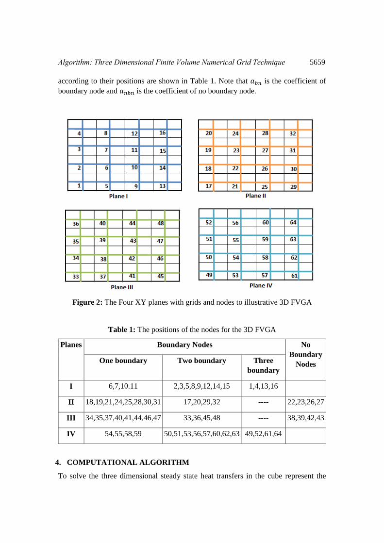
according to their positions are shown in Table 1. Note that 𝑎𝑏𝑛 is the coefficient of

boundary node and 𝑎𝑛𝑏𝑛 is the coefficient of no boundary node.

Figure 2: The Four XY planes with grids and nodes to illustrative 3D FVGA

Table 1: The positions of the nodes for the 3D FVGA

Planes Boundary Nodes No

Boundary

Nodes One boundary Two boundary Three

boundary

I 6,7,10.11 2,3,5,8,9,12,14,15 1,4,13,16

II 18,19,21,24,25,28,30,31 17,20,29,32 ---- 22,23,26,27

III 34,35,37,40,41,44,46,47 33,36,45,48 ---- 38,39,42,43

IV 54,55,58,59 50,51,53,56,57,60,62,63 49,52,61,64

4. COMPUTATIONAL ALGORITHM

To solve the three dimensional steady state heat transfers in the cube represent the

5660 Parag V. Patil, Pravin N. Bhirud and J. S. V. R. Krishna Prasad

equation (7) using finite volume grid technique, proceed as follows.

Algorithm 4.1. Finite Volume Grid Algorithm for Three Dimensional Problems.

If the temperature 𝜃 is the function of 𝑥, 𝑦, 𝑧 and may be constant then

Step 1: For the one boundary nodes

{

𝑎𝑏𝑛 = 0

𝑎𝑛𝑏𝑛 =𝑘𝐴

∆

𝑆 =2𝑘𝐴

∆𝜃

𝑆𝑝 = −2𝑘𝐴

∆

𝑎𝑝 = 𝑎𝑏𝑛 +∑𝑎𝑛𝑏𝑛 − 𝑆𝑝

Step 2: For the Two boundary nodes.

{

𝑎𝑏𝑛 = 0

𝑎𝑛𝑏𝑛 =𝑘𝐴

∆

𝑆 =2𝑘𝐴

∆𝜃1 +

2𝑘𝐴

∆𝜃2

𝑆𝑝 = −2𝑘𝐴

∆−2𝑘𝐴

∆

𝑎𝑝 =∑𝑎𝑏𝑛 +∑𝑎𝑛𝑏𝑛 − 𝑆𝑝

Step 3: For the three boundary nodes

{

𝑎𝑏𝑛 = 0

𝑎𝑛𝑏𝑛 =𝑘𝐴

∆

𝑆 =2𝑘𝐴

∆𝜃1 +

2𝑘𝐴

∆𝜃2 +

2𝑘𝐴

∆𝜃3

𝑆𝑝 = −2𝑘𝐴

∆−2𝑘𝐴

∆−2𝑘𝐴

∆

𝑎𝑝 =∑𝑎𝑏𝑛 +∑𝑎𝑛𝑏𝑛 − 𝑆𝑝

Algorithm: Three Dimensional Finite Volume Numerical Grid Technique 5661

Step 4: For the No boundary nodes

{

𝑎𝑛𝑏𝑛 =

𝑘𝐴

∆𝑆𝜃 = 𝑆𝑝 = 0

𝑎𝑝 =∑𝑎𝑛𝑏𝑛 − 𝑆𝑝

Iteration 1

Step 5: Calculation for Plane I

Set the given vector 𝑎𝑁 = 𝑎, 𝑎𝑃 = 𝑏, 𝑎𝑆 = 𝑐, 𝜃𝑊 = 𝜃𝐸 = 𝜃𝐵 = 𝜃𝑇 = 0 and

𝑎𝑊𝜃𝑊 + 𝑎𝐸𝜃𝐸 + 𝑎𝐵𝜃𝐵 + 𝑎𝑇𝜃𝑇 + 𝑆 = 𝑑

5.1. For 𝑖 = 1, set 𝐴0 = 0 , 𝐵0 = 0 and compute

𝐴1 =𝑐1

𝑏1 − 𝑎1𝐴0 𝑎𝑛𝑑 𝐵1 =

𝑎1𝐵0 + 𝑑1𝑏1 − 𝑎1𝐴0

5.2. For 𝑖 = 2, − − −−, 𝑛 and compute

𝐴𝑖 =𝑐𝑖

𝑏𝑖 − 𝑎𝑖𝐴𝑖−1 𝑎𝑛𝑑 𝐵𝑖 =

𝑎𝑖𝐵𝑖−1 + 𝑑𝑖𝑏𝑖 − 𝑎𝑖𝐴𝑖−1

5.3.For 𝑖 = 𝑛 − − − −1, Set 𝜃𝑛+1 = 0 and compute 𝜃𝑖 = 𝐴𝑖𝜃𝑖+1 + 𝐵𝑖

The End of the First Line

Set the given vectors 𝑎𝑁 = 𝑎, 𝑎𝑃 = 𝑏, 𝑎𝑆 = 𝑐, 𝜃𝐸 = 𝜃𝐵 = 𝜃𝑇 = 0 , 𝜃𝑊 =

𝜃(Result of first line ) and 𝑎𝑊𝜃𝑊 + 𝑎𝐸𝜃𝐸 + 𝑎𝐵𝜃𝐵 + 𝑎𝑇𝜃𝑇 + 𝑆 = 𝑑.

Repeated steps 5.1, 5.2 and 5.3 then get the result of second line.

The End of the Second Line

Set the given vectors 𝑎𝑁 = 𝑎, 𝑎𝑃 = 𝑏, 𝑎𝑆 = 𝑐, 𝜃𝐸 = 𝜃𝐵 = 𝜃𝑇 = 0 , 𝜃𝑊 =

𝜃(Result of second line ) and 𝑎𝑊𝜃𝑊 + 𝑎𝐸𝜃𝐸 + 𝑎𝐵𝜃𝐵 + 𝑎𝑇𝜃𝑇 + 𝑆 = 𝑑.

Repeated steps 5.1, 5.2 and 5.3 then get the result of third line.

The End of the Third Line

Set the given vectors 𝑎𝑁 = 𝑎, 𝑎𝑃 = 𝑏, 𝑎𝑆 = 𝑐, 𝜃𝐸 = 𝜃𝐵 = 𝜃𝑇 = 0 , 𝜃𝑊 =

𝜃(Result of third line ) and 𝑎𝑊𝜃𝑊 + 𝑎𝐸𝜃𝐸 + 𝑎𝐵𝜃𝐵 + 𝑎𝑇𝜃𝑇 + 𝑆 = 𝑑.

Repeated steps 5.1, 5.2 and 5.3 then get the result of fourth line.

The End of the Fourth Line

5662 Parag V. Patil, Pravin N. Bhirud and J. S. V. R. Krishna Prasad

Step 6: Calculation for Plane II

Set the given vectors 𝑎𝑁 = 𝑎, 𝑎𝑃 = 𝑏, 𝑎𝑆 = 𝑐, 𝜃𝐸 = 𝜃𝑊 = 𝜃𝑇 = 0, 𝜃𝐵 =

𝜃(Result of first line-Plane I-Iteration 1) and 𝑎𝑊𝜃𝑊 + 𝑎𝐸𝜃𝐸 + 𝑎𝐵𝜃𝐵 + 𝑎𝑇𝜃𝑇 +

𝑆 = 𝑑.

Repeated steps 5.1, 5.2 and 5.3 then get the result of first line.

The End of the First Line

Set the given vectors 𝑎𝑁 = 𝑎, 𝑎𝑃 = 𝑏, 𝑎𝑆 = 𝑐, 𝜃𝐸 = 𝜃𝑇 = 0 , 𝜃𝑊 = 𝜃(Result of

first line-Plane II-Iteration 1), 𝜃𝐵 = 𝜃(Result of second line-Plane I-Iteration 1),

and 𝑎𝑊𝜃𝑊 + 𝑎𝐸𝜃𝐸 + 𝑎𝐵𝜃𝐵 + 𝑎𝑇𝜃𝑇 + 𝑆 = 𝑑.

Repeated steps 5.1, 5.2 and 5.3 then get the result of second line.

The End of the Second Line

Set the given vectors 𝑎𝑁 = 𝑎, 𝑎𝑃 = 𝑏, 𝑎𝑆 = 𝑐, 𝜃𝐸 = 𝜃𝑇 = 0 , 𝜃𝑊 = 𝜃(Result of

second line-Plane II-Iteration 1 ), 𝜃𝐵 = 𝜃(Result of third line-Plane I-Iteration

1) and 𝑎𝑊𝜃𝑊 + 𝑎𝐸𝜃𝐸 + 𝑎𝐵𝜃𝐵 + 𝑎𝑇𝜃𝑇 + 𝑆 = 𝑑.

Repeated steps 5.1, 5.2 and 5.3 then get the result of third line.

The End of the Third Line

Set the given vectors 𝑎𝑁 = 𝑎, 𝑎𝑃 = 𝑏, 𝑎𝑆 = 𝑐, 𝜃𝐸 = 𝜃𝑇 = 0 , 𝜃𝑊 = 𝜃(Result of

third line –Plane II-Iteration 1), 𝜃𝐵 = 𝜃 (Result of fourth line-Plane I-Iteration

1) and 𝑎𝑊𝜃𝑊 + 𝑎𝐸𝜃𝐸 + 𝑎𝐵𝜃𝐵 + 𝑎𝑇𝜃𝑇 + 𝑆 = 𝑑.

Repeated steps 5.1, 5.2 and 5.3 then get the result of fourth line.

The End of the Fourth Line

Step 7: Calculation for Plane III

Set the given vectors 𝑎𝑁 = 𝑎, 𝑎𝑃 = 𝑏, 𝑎𝑆 = 𝑐, 𝜃𝐸 = 𝜃𝑊 = 𝜃𝑇 = 0, 𝜃𝐵 =

𝜃(Result of first line-Plane II-Iteration 1) and 𝑎𝑊𝜃𝑊 + 𝑎𝐸𝜃𝐸 + 𝑎𝐵𝜃𝐵 +

𝑎𝑇𝜃𝑇 + 𝑆 = 𝑑.

Repeated steps 5.1, 5.2 and 5.3 then get the result of first line.

The End of the First Line

Set the given vectors 𝑎𝑁 = 𝑎, 𝑎𝑃 = 𝑏, 𝑎𝑆 = 𝑐, 𝜃𝐸 = 𝜃𝑇 = 0 , 𝜃𝑊 = 𝜃(Result of

first line-Plane III-Iteration 1), 𝜃𝐵 = 𝜃(Result of second line-Plane II-Iteration

1), and 𝑎𝑊𝜃𝑊 + 𝑎𝐸𝜃𝐸 + 𝑎𝐵𝜃𝐵 + 𝑎𝑇𝜃𝑇 + 𝑆 = 𝑑.

Algorithm: Three Dimensional Finite Volume Numerical Grid Technique 5663

Repeated steps 5.1, 5.2 and 5.3 then get the result of second line.

The End of the Second Line

Set the given vectors 𝑎𝑁 = 𝑎, 𝑎𝑃 = 𝑏, 𝑎𝑆 = 𝑐, 𝜃𝐸 = 𝜃𝑇 = 0 , 𝜃𝑊 = 𝜃(Result of

second line-Plane III-Iteration 1 ), 𝜃𝐵 = 𝜃(Result of third line-Plane II-Iteration

1) and 𝑎𝑊𝜃𝑊 + 𝑎𝐸𝜃𝐸 + 𝑎𝐵𝜃𝐵 + 𝑎𝑇𝜃𝑇 + 𝑆 = 𝑑.

Repeated steps 5.1, 5.2 and 5.3 then get the result of third line.

The End of the Third Line

Set the given vectors 𝑎𝑁 = 𝑎, 𝑎𝑃 = 𝑏, 𝑎𝑆 = 𝑐, 𝜃𝐸 = 𝜃𝑇 = 0 , 𝜃𝑊 = 𝜃(Result of

third line –Plane III-Iteration 2), 𝜃𝐵 = 𝜃 (Result of fourth line-Plane II-Iteration

1) and 𝑎𝑊𝜃𝑊 + 𝑎𝐸𝜃𝐸 + 𝑎𝐵𝜃𝐵 + 𝑎𝑇𝜃𝑇 + 𝑆 = 𝑑.

Repeated steps 5.1, 5.2 and 5.3 then get the result of fourth line.

The End of the Fourth Line

Step 8: Calculation for Plane IV

Set the given vectors 𝑎𝑁 = 𝑎, 𝑎𝑃 = 𝑏, 𝑎𝑆 = 𝑐, 𝜃𝐸 = 𝜃𝑊 = 𝜃𝑇 = 0, 𝜃𝐵 =

𝜃(Result of first line-Plane III-Iteration 1) and 𝑎𝑊𝜃𝑊 + 𝑎𝐸𝜃𝐸 + 𝑎𝐵𝜃𝐵 +

𝑎𝑇𝜃𝑇 + 𝑆 = 𝑑.

Repeated steps 5.1, 5.2 and 5.3 then get the result of first line.

The End of the First Line

Set the given vectors 𝑎𝑁 = 𝑎, 𝑎𝑃 = 𝑏, 𝑎𝑆 = 𝑐, 𝜃𝐸 = 𝜃𝑇 = 0 , 𝜃𝑊 = 𝜃(Result of

first line-Plane IV-Iteration 1), 𝜃𝐵 = 𝜃(Result of second line-Plane III-Iteration

1), and 𝑎𝑊𝜃𝑊 + 𝑎𝐸𝜃𝐸 + 𝑎𝐵𝜃𝐵 + 𝑎𝑇𝜃𝑇 + 𝑆 = 𝑑.

Repeated steps 5.1, 5.2 and 5.3 then get the result of second line.

The End of the Second Line

Set the given vectors 𝑎𝑁 = 𝑎, 𝑎𝑃 = 𝑏, 𝑎𝑆 = 𝑐, 𝜃𝐸 = 𝜃𝑇 = 0 , 𝜃𝑊 = 𝜃(Result of

second line-Plane IV-Iteration 1 ), 𝜃𝐵 = 𝜃(Result of third line-Plane III-

Iteration 1) and 𝑎𝑊𝜃𝑊 + 𝑎𝐸𝜃𝐸 + 𝑎𝐵𝜃𝐵 + 𝑎𝑇𝜃𝑇 + 𝑆 = 𝑑.

Repeated steps 5.1, 5.2 and 5.3 then get the result of third line.

The End of the Third Line

Set the given vectors 𝑎𝑁 = 𝑎, 𝑎𝑃 = 𝑏, 𝑎𝑆 = 𝑐, 𝜃𝐸 = 𝜃𝑇 = 0 , 𝜃𝑊 = 𝜃(Result of

third line –Plane IV-Iteration 2), 𝜃𝐵 = 𝜃 (Result of fourth line-Plane III-

5664 Parag V. Patil, Pravin N. Bhirud and J. S. V. R. Krishna Prasad

Iteration 1) and 𝑎𝑊𝜃𝑊 + 𝑎𝐸𝜃𝐸 + 𝑎𝐵𝜃𝐵 + 𝑎𝑇𝜃𝑇 + 𝑆 = 𝑑.

Repeated steps 5.1, 5.2 and 5.3 then get the result of fourth line.

The End of the Fourth Line

Iteration 2

Step 9: Calculation for Plane I

Set the given vector 𝑎𝑁 = 𝑎, 𝑎𝑃 = 𝑏, 𝑎𝑆 = 𝑐, 𝜃𝑊 = 𝜃𝐵 = 0 , 𝜃𝐸 = 𝜃(Result of

Second line-Plane I Iteration 1) 𝜃𝑇 = 𝜃(Result of first line-Plane II Iteration 1)

,and 𝑎𝑊𝜃𝑊 + 𝑎𝐸𝜃𝐸 + 𝑎𝐵𝜃𝐵 + 𝑎𝑇𝜃𝑇 + 𝑆 = 𝑑.

Repeated steps 5.1, 5.2 and 5.3 then get the result of first line.

The End of the First Line.

Set the given vectors 𝑎𝑁 = 𝑎, 𝑎𝑃 = 𝑏, 𝑎𝑆 = 𝑐, 𝜃𝐵 = 0, 𝜃𝑊 = 𝜃(Result of first

line-Plane I Iteration 2), 𝜃𝐸 = 𝜃(Result of third line-Plane I Iteration 1), 𝜃𝑇 =

𝜃(Result of second line-Plane II Iteration 1), and 𝑎𝑊𝜃𝑊 + 𝑎𝐸𝜃𝐸 + 𝑎𝐵𝜃𝐵 +

𝑎𝑇𝜃𝑇 + 𝑆 = 𝑑.

Repeated steps 5.1, 5.2 and 5.3 then get the result of second line.

The End of the Second Line

Set the given vectors 𝑎𝑁 = 𝑎, 𝑎𝑃 = 𝑏, 𝑎𝑆 = 𝑐, 𝜃𝐵 = 0 , 𝜃𝑊 = 𝜃(Result of

second line-Plane I Iteration 2), 𝜃𝐸 = 𝜃(Result of fourth line-Plane I Iteration

1), 𝜃𝑇 = 𝜃(Result of third line-Plane II Iteration 1), and 𝑎𝑊𝜃𝑊 + 𝑎𝐸𝜃𝐸 +

𝑎𝐵𝜃𝐵 + 𝑎𝑇𝜃𝑇 + 𝑆 = 𝑑.

Repeated steps 5.1, 5.2 and 5.3 then get the result of third line.

The End of the Third Line.

Set the given vectors 𝑎𝑁 = 𝑎, 𝑎𝑃 = 𝑏, 𝑎𝑆 = 𝑐, 𝜃𝐸 = 𝜃𝐵 = 0 , 𝜃𝑊 = 𝜃(Result of

third line-Plane I Iteration 2), 𝜃𝑇 = 𝜃(Result of fourth line-Plane II Iteration 1),

and 𝑎𝑊𝜃𝑊 + 𝑎𝐸𝜃𝐸 + 𝑎𝐵𝜃𝐵 + 𝑎𝑇𝜃𝑇 + 𝑆 = 𝑑.

Repeated steps 5.1, 5.2 and 5.3 then get the result of fourth line.

The End of the Fourth Line

Step 10: Calculation for Plane II

Set the given vectors 𝑎𝑁 = 𝑎, 𝑎𝑃 = 𝑏, 𝑎𝑆 = 𝑐, 𝜃𝑊 = 0, 𝜃𝐸 = 𝜃(Result of

Algorithm: Three Dimensional Finite Volume Numerical Grid Technique 5665

second line-Plane II-Iteration 1),𝜃𝐵 = 𝜃(Result of first line-Plane I Iteration 2),

𝜃𝑇 = 𝜃(Result of first line-Plane III Iteration 1) and 𝑎𝑊𝜃𝑊 + 𝑎𝐸𝜃𝐸 + 𝑎𝐵𝜃𝐵 +

𝑎𝑇𝜃𝑇 + 𝑆 = 𝑑.

Repeated steps 5.1, 5.2 and 5.3 then get the result of first line.

The End of the First Line

Set the given vectors 𝑎𝑁 = 𝑎, 𝑎𝑃 = 𝑏, 𝑎𝑆 = 𝑐, , 𝜃𝑊 = 𝜃(Result of first line-

Plane II-Iteration 2), 𝜃𝐸 = 𝜃(Result of third line-Plane II-Iteration 1), 𝜃𝐵 =

𝜃(Result of second line-Plane I Iteration 2), 𝜃𝑇 = 𝜃(Result of second line-Plane

III Iteration 1), and 𝑎𝑊𝜃𝑊 + 𝑎𝐸𝜃𝐸 + 𝑎𝐵𝜃𝐵 + 𝑎𝑇𝜃𝑇 + 𝑆 = 𝑑.

Repeated steps 5.1, 5.2 and 5.3 then get the result of second line.

The End of the Second Line

Set the given vectors 𝑎𝑁 = 𝑎, 𝑎𝑃 = 𝑏, 𝑎𝑆 = 𝑐, 𝜃𝑊 = 𝜃(Result of second line-

Plane II-Iteration 2), 𝜃𝐸 = 𝜃(Result of fourth line-Plane II-Iteration 1), 𝜃𝐵 =

𝜃(Result of third line-Plane I Iteration 2), 𝜃𝑇 = 𝜃(Result of third line-Plane III

Iteration 1), and 𝑎𝑊𝜃𝑊 + 𝑎𝐸𝜃𝐸 + 𝑎𝐵𝜃𝐵 + 𝑎𝑇𝜃𝑇 + 𝑆 = 𝑑.

Repeated steps 5.1, 5.2 and 5.3 then get the result of third line.

The End of the Third Line

Set the given vectors 𝑎𝑁 = 𝑎, 𝑎𝑃 = 𝑏, 𝑎𝑆 = 𝑐, 𝜃𝐸 = 0, 𝜃𝑊 = 𝜃(Result of third

line –Plane II-Iteration 2), 𝜃𝐵 = 𝜃 (Result of fourth line-Plane I-Iteration 2),

𝜃𝑇 = 𝜃(Result of fourth line-Plane III Iteration 1), and 𝑎𝑊𝜃𝑊 + 𝑎𝐸𝜃𝐸 +

𝑎𝐵𝜃𝐵 + 𝑎𝑇𝜃𝑇 + 𝑆 = 𝑑.

Repeated steps 5.1, 5.2 and 5.3 then get the result of fourth line.

The End of the Fourth Line

Step 11: Calculation for Plane III

Set the given vectors 𝑎𝑁 = 𝑎, 𝑎𝑃 = 𝑏, 𝑎𝑆 = 𝑐, 𝜃𝑊 = 0 , 𝜃𝐸 = 𝜃(Result of

second line-Plane III-Iteration 1), 𝜃𝐵 = 𝜃(Result of first line-Plane II-Iteration

2), 𝜃𝑇 = 𝜃(Result of first line-Plane IV-Iteration 1) and 𝑎𝑊𝜃𝑊 + 𝑎𝐸𝜃𝐸 +

𝑎𝐵𝜃𝐵 + 𝑎𝑇𝜃𝑇 + 𝑆 = 𝑑.

Repeated steps 5.1, 5.2 and 5.3 then get the result of first line.

The End of the First Line

Set the given vectors 𝑎𝑁 = 𝑎, 𝑎𝑃 = 𝑏, 𝑎𝑆 = 𝑐, 𝜃𝑊 = 𝜃(Result of first line-Plane

5666 Parag V. Patil, Pravin N. Bhirud and J. S. V. R. Krishna Prasad

III-Iteration 2), 𝜃𝐸 = 𝜃(Result of third line-Plane III-Iteration 1), 𝜃𝐵 =

𝜃(Result of second line-Plane II-Iteration 2), 𝜃𝑇 = 𝜃(Result of second line-

Plane IV-Iteration 1) and 𝑎𝑊𝜃𝑊 + 𝑎𝐸𝜃𝐸 + 𝑎𝐵𝜃𝐵 + 𝑎𝑇𝜃𝑇 + 𝑆 = 𝑑.

Repeated steps 5.1, 5.2 and 5.3 then get the result of second line.

The End of the Second Line

Set the given vectors 𝑎𝑁 = 𝑎, 𝑎𝑃 = 𝑏, 𝑎𝑆 = 𝑐, 𝜃𝑊 = 𝜃(Result of second line-

Plane III-Iteration 2), 𝜃𝐸 = 𝜃(Result of fourth line-Plane III-Iteration 1), 𝜃𝐵 =

𝜃(Result of third line-Plane II-Iteration 2), 𝜃𝑇 = 𝜃(Result of third line-Plane

IV-Iteration 1) and 𝑎𝑊𝜃𝑊 + 𝑎𝐸𝜃𝐸 + 𝑎𝐵𝜃𝐵 + 𝑎𝑇𝜃𝑇 + 𝑆 = 𝑑.

Repeated steps 5.1, 5.2 and 5.3 then get the result of third line.

The End of the Third Line

Set the given vectors 𝑎𝑁 = 𝑎, 𝑎𝑃 = 𝑏, 𝑎𝑆 = 𝑐, 𝜃𝐸 = 0 , 𝜃𝑊 = 𝜃(Result of third

line –Plane III-Iteration 2), 𝜃𝐵 = 𝜃 (Result of fourth line-Plane II-Iteration 2),

𝜃𝑇 = 𝜃(Result of fourth line-Plane IV-Iteration 1), and 𝑎𝑊𝜃𝑊 + 𝑎𝐸𝜃𝐸 +

𝑎𝐵𝜃𝐵 + 𝑎𝑇𝜃𝑇 + 𝑆 = 𝑑.

Repeated steps 5.1, 5.2 and 5.3 then get the result of fourth line.

The End of the Fourth Line

Step 12: Calculation for Plane IV

Set the given vectors 𝑎𝑁 = 𝑎, 𝑎𝑃 = 𝑏, 𝑎𝑆 = 𝑐, 𝜃𝑊 = 𝜃𝑇 = 0 , 𝜃𝐸 = 𝜃(Result of

second line-Plane IV-Iteration 1), 𝜃𝐵 = 𝜃(Result of first line-Plane III-Iteration

2), and 𝑎𝑊𝜃𝑊 + 𝑎𝐸𝜃𝐸 + 𝑎𝐵𝜃𝐵 + 𝑎𝑇𝜃𝑇 + 𝑆 = 𝑑.

Repeated steps 5.1, 5.2 and 5.3 then get the result of first line.

The End of the First Line.

Set the given vectors 𝑎𝑁 = 𝑎, 𝑎𝑃 = 𝑏, 𝑎𝑆 = 𝑐, 𝜃𝑇 = 0 , 𝜃𝑊 = 𝜃(Result of first

line-Plane IV-Iteration 2), 𝜃𝐸 = 𝜃(Result of third line-Plane IV-Iteration 1),

𝜃𝐵 = 𝜃(Result of second line-Plane III-Iteration 2), and 𝑎𝑊𝜃𝑊 + 𝑎𝐸𝜃𝐸 +

𝑎𝐵𝜃𝐵 + 𝑎𝑇𝜃𝑇 + 𝑆 = 𝑑.

Repeated steps 5.1, 5.2 and 5.3 then get the result of second line.

The End of the Second Line

Set the given vectors 𝑎𝑁 = 𝑎, 𝑎𝑃 = 𝑏, 𝑎𝑆 = 𝑐, 𝜃𝑇 = 0 , 𝜃𝑊 = 𝜃(Result of

second line-Plane IV-Iteration 2), 𝜃𝐸 = 𝜃(Result of fourth line-Plane IV-

Algorithm: Three Dimensional Finite Volume Numerical Grid Technique 5667

Iteration 1), 𝜃𝐵 = 𝜃(Result of third line-Plane III-Iteration 2), and 𝑎𝑊𝜃𝑊 +

𝑎𝐸𝜃𝐸 + 𝑎𝐵𝜃𝐵 + 𝑎𝑇𝜃𝑇 + 𝑆 = 𝑑.

Repeated steps 5.1, 5.2 and 5.3 then get the result of third line.

The End of the Third Line

Set the given vectors 𝑎𝑁 = 𝑎, 𝑎𝑃 = 𝑏, 𝑎𝑆 = 𝑐, 𝜃𝐸 = 𝜃𝑇 = 0 , 𝜃𝑊 = 𝜃(Result of

third line –Plane IV-Iteration 2), 𝜃𝐵 = 𝜃 (Result of fourth line-Plane III-

Iteration 2) and 𝑎𝑊𝜃𝑊 + 𝑎𝐸𝜃𝐸 + 𝑎𝐵𝜃𝐵 + 𝑎𝑇𝜃𝑇 + 𝑆 = 𝑑.

Repeated steps 5.1, 5.2 and 5.3 then get the result of fourth line.

The End of the Fourth Line.

The entire iteration 2 procedure is repeated until a converged solution is obtained. For

the three dimensional problem, this algorithm proposed name as Finite Volume Grid

Algorithm (3DFVGA).

5. AN ILLUSTRATIVE EXAMPLE

Let us consider the three dimensional steady state heat equation as shown by equation

(7) with dirichlet boundary conditions

𝜃(0, 𝑦, 𝑧) = 𝜃(𝑥, 0, 𝑦) = 𝜃(𝑥, 𝑦, 0) = 0

𝜃(1, 𝑦, 𝑧) = 𝑦𝑧

𝜃(𝑥, 1, 𝑧) = 𝑧𝑥

𝜃(𝑥, 𝑦, 1) = 𝑥𝑦

The analytic solution of this problem is given by 𝜃(𝑥, 𝑦, 𝑧) = 𝑥𝑦𝑧 and its converged

numerical solution is obtained after seventh iterations as shown in Table 2. In figure 1,

three dimensional solution region cube is shown and is divided into four plane as shown

in figure 2. The thermal conductivity of the cube material is 𝑘 = 1000 w/m/k. Use a

uniform grid size ∇𝑥 = ∇𝑦 = ∇𝑧 = 0.25 𝑚.

The input value with the boundary conditions of Figure 3. The Figure 4 shows that the

input boundary data for the spreadsheet implementation to the known nodes potentials

at the boundary of the three dimensional solution region. The coefficient and the source

terms of the finite volume discretized equations for all the nodes are calculated plane

by plane along the north-south lines as same to the two dimension case [12] and the

orange, green ,blue and yellow colour indicates that one ,two ,three and no boundary

nodes of the figure 4.

5668 Parag V. Patil, Pravin N. Bhirud and J. S. V. R. Krishna Prasad

Figure 3: Input section of spreadsheet implementation of the 3DFVGA

Algorithm: Three Dimensional Finite Volume Numerical Grid Technique 5669

Figure 4- The Finite Volume discretization with respective Plane I-IV to illustrate the

3DFVGA

The entire iteration plane by plane procedure is now repeated until a converged solution

is obtained. The next all steps of this algorithm should be followed as per two

dimensional case [12]. The numerical solution of such type of linear system has been

obtained after seven iterations and which shows in Table 2.

Table 2: A Comparison between Finite Volume Numerical Solution after 7th iteration

and Analytical solutions

Planes I II III IV

Nodes FVT Analytic FVT Analytic FVT Analytic FVT Analytic

1 0.0019 0.0020 0.0064 0.0059 0.0097 0.0098 0.0136 0.0137

2 0.0055 0.0059 0.0176 0.0176 0.0288 0.0293 0.0408 0.0410

3 0.0101 0.0098 0.0283 0.0293 0.0480 0.0488 0.0680 0.0684

4 0.0123 0.0137 0.0395 0.0410 0.0677 0.0684 0.0954 0.0957

5 0.0055 0.0059 0.0197 0.0176 0.0295 0.0293 0.0409 0.0410

6 0.0174 0.0176 0.0546 0.0527 0.0877 0.0879 0.1225 0.1230

7 0.0305 0.0293 0.0867 0.0879 0.1453 0.1465 0.2041 0.2051

8 0.0400 0.0410 0.1186 0.1230 0.2033 0.2051 0.2858 0.2871

9 0.0090 0.0098 0.0329 0.0293 0.0495 0.0488 0.0684 0.0684

10 0.0305 0.0293 0.0920 0.0879 0.1470 0.1465 0.2050 0.2051

11 0.0529 0.0488 0.1463 0.1465 0.2435 0.2441 0.3415 0.3418

5670 Parag V. Patil, Pravin N. Bhirud and J. S. V. R. Krishna Prasad

12 0.0600 0.0684 0.1985 0.2051 0.3403 0.3418 0.4781 0.4785

13 0.0165 0.0137 0.0435 0.0410 0.0687 0.0684 0.0957 0.0957

14 0.0400 0.0410 0.1260 0.1230 0.2052 0.2051 0.2867 0.2871

15 0.0700 0.0684 0.2057 0.2051 0.3417 0.3418 0.4784 0.4785

16 0.0901 0.0957 0.2819 0.2871 0.4776 0.4785 0.6698 0.6699

6. CONCLUSION

In this paper, finite volume numerical grid technique for steady state heat flow problems

have been studied and obtained the numerical solution using proposed algorithm, via

3DFVGA. The proposed algorithm described here is a very effective, gratuitous and

easy to implement in high-priced mathematical software such as MAPLE,

MATHEMATICS and MATLAB for solving the finite volume structured grid of

discretized equations which appear in CFD problems and many engineering

application.

REFERENCES

[1] Erwin Kreyszig, 2012, Advanced Engineering Mathematics, John Wiley and

Sons, New York, 10th edition.

[2] Patil Parag V and J. S. V. R Krishna Prasad, 2013, “Numerical Solution for

Two Dimensional Laplace Equation with Dirichlet Boundary Conditions”,

International Organization of Scientific Research- Journal of Mathematics,

6(4), pp 66-75.

[3] Lau Mark A and Kuruganty Sastry P., 2010, “Spreadsheet Implementations for

Solving Boundary-Value Problems in Electromagnetic”, Spreadsheets in

Education (eJSiE), 4(1).

[4] Necat Ozisik, M., 1985, Heat Transfer: A Basic Approach, McGraw-Hill Book

Company, 1st edition.

[5] Patil Parag V and J. S. V. R Krishna Prasad, 2013, “Solution of Laplace

Equation using Finite Element Method”, Pratibha: International Journal of

Science, Spirituality, Business and Technology, 2(1), pp 40-46.

[6] Patil Parag V and J. S. V. R Krishna Prasad, 2014, “A numerical grid and grid

less (Meshless) techniques for the solution of 2D Laplace equation”, Advances

in Applied Science Research, Pelagia Research Library, 5(1), pp 150-155.

[7] Sadiku M. N. O., 2006, Elements of Electromagnetics, Oxford University

Press, New York, 4th edition.

[8] Versteeg H. K. and Malalasekera W., 1995, An Introduction to computational

Algorithm: Three Dimensional Finite Volume Numerical Grid Technique 5671

fluid dynamics: The finite volume method, Longman Scientific and Technical,

1th edition.

[9] EI-Mikkawy M. E. A., 2004, “A Fast algorithm for evaluating nth order tri

diagonal determinants”, J. Comput. Appl. Math., 166, pp 581-584.

[10] EI-Mikkawy M. E. A., 2005, “A new computational algorithm for solving

periodic tridiagonal line systems”, Appl. Math. Comput. 161(2), pp 691-696.

[11] Karawia A. A., 2007, “Two Algorithm for solving a general backward tri-

diagonal linear systems”, Applied Mathematics and Computation, 194(2), pp

534-539.

[12] Patil Parag V and J. S. V. R Krishna Prasad, 2014, “Algorithm for Finite

Volume Numerical Grid Technique”, Cyber Times International Journal of

Technology and Management, 7(2), pp 63-69.

5672 Parag V. Patil, Pravin N. Bhirud and J. S. V. R. Krishna Prasad