Algorithm Selection via Ranking

Richard J. Oentaryo and Stephanus Daniel Handoko and Hoong Chuin LauLiving Analytics Research Centre, School of Information Systems

Singapore Management University, Singapore 178902{roentaryo, dhandoko, hclau}@smu.edu.sg

Abstract

The abundance of algorithms developed to solve differ-ent problems has given rise to an important researchquestion: How do we choose the best algorithm for agiven problem? Known as algorithm selection, this is-sue has been prevailing in many domains, as no singlealgorithm can perform best on all problem instances.Traditional algorithm selection and portfolio construc-tion methods typically treat the problem as a classifica-tion or regression task. In this paper, we present a newapproach that provides a more natural treatment of algo-rithm selection and portfolio construction as a rankingtask. Accordingly, we develop a Ranking-Based Algo-rithm Selection (RAS) method, which employs a sim-ple polynomial model to capture the ranking of differ-ent solvers for different problem instances. We devisean efficient iterative algorithm that can gracefully opti-mize the polynomial coefficients by minimizing a rank-ing loss function, which is derived from a sound prob-abilistic formulation of the ranking problem. Experi-ments on the SAT 2012 competition dataset show thatour approach yields competitive performance to that ofmore sophisticated algorithm selection methods.

IntroductionOver the years, a myriad of algorithms and heuristics havebeen developed to solve various problems and tasks. Thisbrings about an important research question: How do we de-termine which algorithm is the best suited for a given prob-lem? This issue has been pivotal in many problem domains,such as machine learning, constraint satisfaction, and combi-natorial optimization. One of the most widely studied prob-lems related to this issue is the propositional satisfiabilityproblem (SAT) (Cook 1971), and a plethora of algorithms(i.e., solvers) have been devised to solve the SAT probleminstances. Such solvers offer a wider range of practical use,as many problems in artifical intellgence and computer sci-ence can be naturally mapped into SAT tasks.

It is often the case, however, that one solver performs bet-ter at tackling some problem instances from a given class,but is substantially worse on other instances. Practitionersare thus faced with a challenging algorithm selection prob-

Copyright c� 2015, Association for the Advancement of ArtificialIntelligence (www.aaai.org). All rights reserved.

lem (Rice 1976): Which solver(s) should be executed to min-imize some performance objective (e.g., expected runtime)?A popular answer is to evaluate the performance of each can-didate solver on a representative set of problem instances,and then use only the solver that yields the best performance.We refer this as the single-best (SB) strategy. Unfortunately,this is not necessarily the best way, as different solvers areoften complementary. That is, the SB strategy would ignoresolvers that are not competitive on average but nonethelessgive good performance on specific instances.

On the other hand, an ideal solution to the algorithm selec-tion problems is to have an oracle that knows which solverswill perform the best on each problem instance. The oraclesurely would give better results than the SB strategy, servingas the theoretical upper bound of the solvers’ performance.Unfortunately, such perfect oracle is not available for SAT(or any other hard) problems, as it is hardly possible to knowa solver’s performance on a new instance exactly without ac-tually executing it. This motivates the development of algo-rithm selection methods that serve as heuristic approxima-tions of the oracle. A prime example is the empirical hard-ness model (Leyton-Brown, Nudelman, and Shoham 2002;Nudelman et al. 2004) adopted by SATZilla, an algorithmselection method that has won several annual SAT competi-tions (Xu et al. 2008; 2012).

Recently, it has been shown that we can exploit the com-plementarity of the solvers by combining them into an algo-rithm portfolio (Huberman, Lukose, and Hogg 1997; Gomesand Selman 2001). Such portfolio may include methods thatpick a single solver for each problem instance (Guerri andMilano 2004; Xu et al. 2008), methods that makes online de-cisions to switch between solvers (Carchrae and Beck 2005;Samulowitz and Memisevic 2007), and methods that executemultiple solvers independently per instance, either in par-allel, sequentially, or partly sequential/parallel (Gomes andSelman 2001; Gagliolo and Schmidhuber 2006; Streeter andSmith 2008; Kadioglu et al. 2011). A common trait amongthese methods is that they employ regression or classifica-tion methods to build an efficient predictor of a solver’s per-formance for each problem instance, given the instance’sfeatures and solver’s performance history (O’Mahony et al.2008; Xu et al. 2012; Malitsky et al. 2013).

While showing successes to some extent, the contem-porary regression- or classification-based algorithm selec-

tion methods are not designed to directly capture the notionof preferability among different solvers for a given prob-lem instance. It is more natural to pose algorithm selec-tion as a ranking problem. For instance, when constructinga sequential algorithm portfolio, we are usually interestedin finding the correct ordering of the solvers so as to de-cide which solvers should be run first and which one later.Contemporary regression-based methods, such as (Xu et al.2008)), typically use pointwise loss function (e.g., squareloss), which is often biased toward problem instances withmore data, that is solved cases in this context. Meanwhile,the classification-based methods, such as (Xu et al. 2012),does not warrant a unique ordering of the solvers, that isclassification (voting) easily leads to ties between solvers,and it is not clear which one should be prioritized first.

Instead of further pursuing regression or classification ap-proach, we take on a new interpretation of algorithm selec-tion and portfolio construction as a ranking task. To realizethis, we propose in this paper a Ranking-based AlgorithmSelection (RAS) methodology, which learns the appropri-ate (unique) ordering of solvers so as to identify the top Kbest solvers for a given problem instance. To our best knowl-edge, RAS is the first approach that is designed to directlyoptimize a ranking objective function suitable for algorithmselection (and in turn portfolio construction) task.

We summarize our main contributions as follows:• We develop a ranking polynomial model that can capture

the rich, nonlinear interactions between problem instanceand solver features. We then extend its use to model theordering of solvers for a specific problem instance.

• We devise an efficient iterative learning procedure for op-timizing a ranking loss function, which is derived froma sound probabilistic formulation of preferability amongdifferent solvers for a specific problem instance.

• We evaluate the efficacy of our RAS approach throughextensive experiments on the SAT 2012 competition data.The results show that RAS outperforms the single-beststrategy and gives competitive performance to that ofSATZilla and random forest-based selection method.

Related WorkAlgorithm selection has been studied in different contexts(Gomes and Selman 1997) and focused on methods that gen-erate or manage a portfolio of solvers. SATZilla is a suc-cessful algoritm selection strategy that utilizes an empiricalhardness model (Xu et al. 2008), and more recently a cost-sensitive random forest classifier (Xu et al. 2012). The algo-rithm selection in SATZilla aims at building a computation-ally inexpensive predictor of a solver’s runtime or class labelon a given problem instance based on features of the instanceand the solver’s past performance. This ability serves as abasis for building an algorithm portfolio that optimizes someobjective function (e.g., percentage of instances solved).

Gagliolo and Schmidhuber (2006) proposed another run-time prediction strategy called GambleTA. The idea was toallocate time to each algorithm online in the form of a banditproblem. While approaches like SATZilla need offline train-ing, this method does training online and perform an online

selection of algorithms. CPHydra (O’Mahony et al. 2008)accommodates case-based reasoning to perform algorithmselection for runtime prediction. More recently, Malitsky etal. (2013) proposed a new algorithm selection method basedon cost-sensitive hierarchical clustering model.

On a different track, several works have been developedthat treat algorithm selection as a recommendation prob-lem. These methods typically use collaborative filtering (CF)methods that adopt a low-rank assumption. That is, the al-gorithm performance matrix can be well-approximated by acombination of low-rank matrices. In (Stern et al. 2010), aBayesian CF model was developed for algorithm selection.As a base model, it employs Matchbox (Stern, Herbrich, andGraepel 2009), a probabilistic recommender system basedon bilinear rating CF model. In a similar vein, Misir andSebag (2013) proposed a CF model based on matrix factor-ization. However, a major shortcoming of these approachesis their reliance on the low-rank assumption, which may nothold for algorithm performance data. Moreover, for matrixfactorization-based approach, an extra effort is needed tobuild a separate surrogate model for handling new probleminstances (i.e., cold-start issue) (Misir and Sebag 2013).

In this work, we develop the RAS methodology that de-viates from existing approaches by treating algorithm selec-tion (and portfolio construction) as a ranking task. At thecore of RAS is a probabilistic ranking model that is sim-pler than sophisticated algorithm selection methods in, e.g.,SATZilla, and does not rely on low-rank assumption or aseparate mechanism for handling novel problem instances.

Proposed ApproachPolynomial ModelOur RAS approach utilizes as its base a polynomial modelthat captures the rich interaction between problem instancefeatures and solver features. For an instance p and a solver s,we denote their feature vectors as ~p = [p

1

, . . . , pi

, . . . , pI

]

and ~s = [s1

, . . . , sj

, . . . , sJ

], where I and J are the totalnumbers of instance and solver features, respectively. Usingthis notation, we define our polynomial model as follows:

fp,s

(⇥) =

IX

i=1

JX

j=1

pi

sj

0

@↵i,j

+

X

i

0 6=i

pi

0�i,i

0,j

1

A (1)

where ⇥ is the set of all model parameters (i.e., polyno-mial coefficients) ↵

i,j

and �i,i

0j

that we want to learn. Theterm f

p,s

(⇥) thus refers to the preference score of a giveninstance-solver pair (p, s). We also note that p

i

sj

and pi

pi

0sj

can be regarded as the order-2 and order-3 interaction termsbetween the features of instance p and solver s respectively,and the polynomial coefficients ↵

i,j

and �i,i

0,j

are the cor-responding interaction weights.

Without loss of generality, we consider a setting wherebywe are given a set of numeric features to represent a prob-lem instance, but there is no explicit feature provided about agiven solver. For this, we construct real-valued feature vec-tor ~p 2 RI to describe an instance, and binary feature vector~s 2 {0, 1}J for a solver. We use one-hot encoding scheme toconstruct the binary vector, i.e., ~s = [0, . . . , 1, . . . , 0], wherethe position of the “1” uniquely identifies a solver.

Ranking DesiderataIn this work, we propose a new take on algorithm selectionas a ranking task. Let P and S be the sets of all problem in-stances and all solvers respectively. The algorithm selectiontask is to provide an instance p 2 P with a total ranking >

p

of all solvers s 2 S. We note that a sound total ranking >p

needs to fulfill several criteria (Rendle et al. 2009):

8s, s0 2 S : s 6= s0 ) s >p

s0 _ s0 >p

s (2)8s, s0 2 S : s >

p

s0 ^ s0 >p

s) s = s0 (3)8s, s0, s00 2 S : s >

p

s0 ^ s0 >p

s00 ) s >p

s00 (4)

The formulae (2)–(4) refer to the totality (i.e., s and s0

should be comparable), anti-symmetry (i.e., unless s = s0,s and s0 should have different ranks), and transitivity prop-erties (i.e., if s ranks higher than s0 and s0 ranks higher thans00, then s should rank higher than s00) properties, respec-tively (Davey and Priestley 2002; Rendle et al. 2009).

Under this notation, the RAS model essentially learns torank solvers based on the following training set D:

D = {(p, s, s0)|s, s0 2 S ^ s >p

s0 ^ s 6= s0} (5)

where each triplet (p, s, s0) 2 D means that problem in-stance p prefers solver s over solver s0. Notably, our goalis to find the ordering of only the top K solvers, i.e., the Ksolvers with the lowest runtime on a given instance. Thus,our training data only include the triplets (p, s, s0) such thats performs better than s0 and s is among the top K solvers.This seemingly biased approach turns out to be beneficial inpractice, as in the end we hardly care about the other solversthat are not in the top K list. Empirically, we also find thatthis approach gives faster training and better results com-pared to including all solvers s that are better than s0.

Probabilistic FoundationWe now present our probabilistic formulation of algorithmselection as ranking task. For a problem instance p, we de-fine the likelihood P (s >

p

s0|⇥) for ranking >p

of solvers,and prior for the polynomial coefficients P (⇥). Under theBayesian framework, finding the correct ranking of solverss is equivalent to maximizing the posterior probability:

P (⇥| >p

) =

P (>p

|⇥)P (⇥)

P (>p

)

/ P (>p

|⇥)P (⇥) (6)

where the denominator P (>p

) is independent from ⇥.In this work, we shall assume that: 1) all problem in-

stances p are independent from one another; and 2) the or-dering of each solver pair (s, s0) for an instance p is indepen-dent from that of every other pair. Using these assumptions,we can express the likelihood P (>

p

|⇥) as:

P (>p

|⇥) =

Y

(p,s,s

0)2P⇥S⇥S

P (s >p

s0|⇥)

I[(p,s,s

0)2D]

⇥ (1� P (s >p

s0|⇥))

I[(p,s,s

0)/2D] (7)

where I[x] is the indicator function (i.e., 1 if condition x istrue, and 0 otherwise). In turn, due to the totality (2) and anti-symmetry (3) properties of a sound ranking, we can simplify

the likelihood P (>p

|⇥) into:

P (>p

|⇥) =

Y

(p,s,s

0)2D

P (s >p

s0|⇥) (8)

Next, we define the probability that an instance p preferssolver s over solver s0 as:

P (s >p

s0|⇥) = �(fp,s,s

0(⇥)) (9)

where �(x) = 1

1+exp(�x)

is the logistic (sigmoid) function,and f

p,s,s

0(⇥) refers to the preferability of solver s over s0

for instance p. In order to satisfy all the three properties (2)–(4), we choose to decompose f

p,s,s

0(⇥) into:

fp,s,s

0(⇥) = f

p,s

(⇥)� fp,s

0(⇥) (10)

where fp,s

(⇥) is the preference score given by (1). That is,we define the preferability f

p,s,s

0(⇥) as the difference be-

tween the preference scores of two solvers s and s0.Lastly, we complete the Bayesian formulation by comput-

ing the prior P (⇥). In this work, we choose a Gaussian priorwith zero mean and diagonal covariance matrix:

P (⇥) / exp

��

2

k⇥k2�

(11)

where k⇥k2 =

Pi

Pj

↵2

i,j

+

Pi

Pi

0P

j

�2

i,i

0,j

and � isthe inverse variance of the Gaussian prior distribution.

Combining the likelihood (8) and prior (11), we can thencompute the posterior distribution P (⇥| >

p

) as:

P (⇥| >p

) /Y

(p,s,s

0)

�(fp,s,s

0(⇥)) exp

��

2

k⇥k2�

(12)

By taking the negative logarithm of the posterior, we canfinally derive the optimization criterion L for our RASmethod, hereafter called the ranking loss:

L = �X

(p,s,s

0)

ln(�(fp,s,s

0(⇥))) +

�

2

k⇥k2 (13)

The optimal ranking >p

can in turn be attained by findingthe polynomial coefficients ⇥ that minimize L. It is worthnoting that L is a convex function and a global optima existsfor such function. Also, the regularization term k⇥k2 servesto penalize large (magnitude) values of the coefficients ↵

i,j

and �i,i

0,j

, thereby reducing the risk of data overfitting.

Learning ProcedureTo minimize L, we adopt an efficient stochastic gradient de-scent (SGD) procedure, which provides stochastic approx-imation of the batch (full) gradient descent method. Thebatch method leads to a “correct” optimization direction, butits convergence is often slow. That is, we have O(|S|⇥ |S|)triplets in the training data D, and so calculating the full gra-dient for each polynomial coefficient will be expensive.

In the SGD approach, instead of computing the full gradi-ent of the overall loss L for all triplets, we update the poly-nomial coefficients based only on sample-wise loss L

p,s,s

0 :

Lp,s,s

0= � ln(�(f

p,s,s

0(⇥))) +

�

2

k⇥k2 (14)

Algorithm 1 SGD Procedure for Ranking OptimizationInput: Training data D, regularization parameter �, learn-

ing rate ⌘, maximum iterations Tmax

Output: Polynomial coefficients ⇥ = {↵i,j

} [ {�i,i

0,j

}1: Initialize all ↵

i,j

and �i,i

0,j

to small random values2: repeat3: Shuffle the order of all triplets in D4: for each triplet (p, s, s0) from the shuffled D do5: Compute �

p,s,s

0(⇥) � (f

p,s

0(⇥)� f

p,s

(⇥))

6: Compute residue � �p,s,s

0 � 1

7: for each feature pair (sj

, s0j

) of solvers s, s0 do8: Compute �s

j

sj

� s0j

9: for each feature pi

of instance p do10: ↵

i,j

↵i,j

� ⌘ [�pi

�sj

+ �↵i,j

]

11: for each feature pi

0 (i0 6= i) of instance p do12: �

i,i

0,j

�i,i

0,j

� ⌘ [�pi

pi

0�s

j

+ ��i,i

0,j

]

13: end for14: end for15: end for16: end for17: until maximum iterations T

max

To minimize Lp,s,s

0 , we can compute the gradient of the lossfunction with respect to each coefficient ↵

i,j

and �i,i

0,j

:

@Lp,s,s

0

@↵i,j

=

@

@↵i,j

(� ln(�(fp,s,s

0(⇥)))) + �↵

i,j

= (�(fp,s,s

0(⇥))� 1) p

i

�sj

+ �↵i,j

(15)@L

p,s,s

0

@�i,i

0,j

=

@

@�i,i

0,j

(� ln(�(fp,s,s

0(⇥)))) + ��

i,i

0,j

= (�(fp,s,s

0(⇥))� 1) p

i

pi

0�s

j

+ ��i,i

0,j

(16)

where �sj

= sj

� s0j

refers to the jth feature differencebetween two solvers s and s0.

This leads to the following update formulae for the poly-nomial coefficients ↵

i,j

and �i,i

0,j

:

↵i,j

↵i,j

� ⌘ [�pi

�sj

+ �↵i,j

] (17)�i,i

0,j

�i,i

0,j

� ⌘ [�pi

pi

0�s

j

+ ��i,i

0,j

] (18)

where ⌘ 2 [0, 1] is a (user-specified) learning rate, and � =

�(fp,s,s

0(⇥))� 1 is the (common) residue term.

Algorithm 1 summarizes our SGD learning procedure forminimizing the ranking loss L in the RAS framework. Theparameter updates take place in lines 7–15, and can be doneefficiently by “caching” the residue term � before enteringthe update loop (see line 6). Further speed-up can be ob-tained by exploiting the sparsity of the (binary) solver fea-ture vector ~s, owing to the one-hot encoding scheme. Ac-cordingly, the (worst) time complexity of the coefficient up-dates in each iteration is O(|D|⇥ I2), where |D| is the totalnumber of data samples/triplets (p, s, s0) and I is the num-ber of problem instance features. The memory requirementof our approach is also quite modest; we only need to storethe model parameters ⇥ with a complexity of O(I2 ⇥ J),where J is the number of solver features. We repeat the SGDprocedure for a maximum of T

max

iterations.

Prediction PhaseUpon completion of the SGD learning process, we wouldhave obtained the polynomial coefficients ⇥ that minimizethe ranking loss L. Using the learned polynomial model, wecan then predict the ranking of different solvers s for a newproblem instance p. This can be done by computing the pref-erence score f

p,s

(⇥) for a given (p, s) pair. Accordingly, fordifferent solvers s applied to problem instance p, we canrank them in a descending order of f

p,s

(⇥), and pick the topK solvers as our recommendation.

ExperimentsDatasetFor our experiments, we use the SAT 2012 datasets suppliedby the UBC group1, after SATZilla won the SAT 2012 Chal-lenge. Table 1 summarizes the datasets. In total, there aresix datasets, which are divided into three instance categoriesand two phase groups. The instance categories include hand-crafted (HAND), industrial application (INDU), and random(RAND). The two phase groups differ mainly in the solversets and the execution time limits. Solvers from the Phase 1datasets were tested with a time limit of 1200 seconds (12S),while those from Phase 2 were run up to 5000 seconds (50S).Note that the solvers in Phase 2 are a subset of the solversin Phase 1, i.e., solvers in Phase 2 are those that performedwell and passed Phase 1 of the competition.

Each dataset is represented as an instance-solver matrix.An element in the matrix contains the runtime of a solveron a given problem instance, if the solver is able to solvethe instance within the time limit. Otherwise, the elementis treated as unsolved, and encoded as “1201” for Phase 1and “5001” for Phase 2. Following Malitsky’s setup2, we re-moved all unsolvable problem instances, i.e., instances thatcould not be solved by any solver within the time limit. Lastbut not least, problem instances are characterized by the 125features the UBC team proposed (option -base), while forsolvers we used a binary feature representation obtained viaone-hot encoding (as described in “Proposed Approach”).

EvaluationAs our evaluation metrics, we use Hit @ Top K (denoted asHit@K) and Mean Average Precision @ Top K (denoted asMAP@K), the well-known ranking metrics in informationretrieval community (Baeza-Yates and Ribeiro-Neto 1999).Both metrics measure the prediction quality for each rankedlist of solvers (sorted in descending order) that is returnedfor a problem instance p. The Hit@K metric refers to thenumber of problem instances successfully solved, assumingthat at least one solver that can solve a given problem in-stance exists at the top K of the ranked list.

To obtain MAP@K, we first need to compute the Aver-age Precision @ top K, i.e., AP(p,K) =

PKi=1 P (i,p)⇥rel(i)PK

i=1 rel(i,p)

,

where rel(i, p) is a binary term indicating whether the ith

retrieved solver has solved problem instance p or not, and

1http://www.cs.ubc.ca/labs/beta/Projects/ SATzilla2http://4c.ucc.ie/ ymalitsky/APBS.html

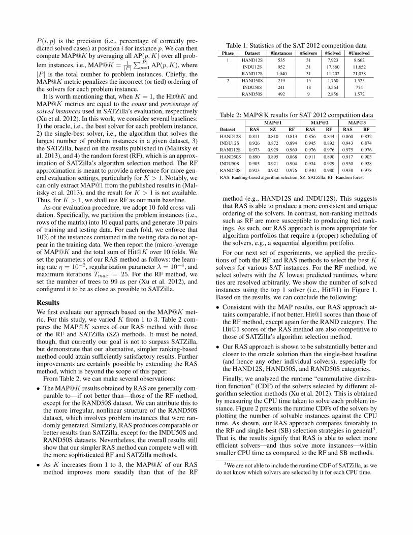
P (i, p) is the precision (i.e., percentage of correctly pre-dicted solved cases) at position i for instance p. We can thencompute MAP@K by averaging all AP(p,K) over all prob-lem instances, i.e., MAP@K =

1

|P |P|P |

p=1

AP(p,K), where|P | is the total number fo problem instances. Chiefly, theMAP@K metric penalizes the incorrect (or tied) ordering ofthe solvers for each problem instance.

It is worth mentioning that, when K = 1, the Hit@K andMAP@K metrics are equal to the count and percentage ofsolved instances used in SATZilla’s evaluation, respectively(Xu et al. 2012). In this work, we consider several baselines:1) the oracle, i.e., the best solver for each problem instance,2) the single-best solver, i.e., the algorithm that solves thelargest number of problem instances in a given dataset, 3)the SATZilla, based on the results published in (Malitsky etal. 2013), and 4) the random forest (RF), which is an approx-imation of SATZilla’s algorithm selection method. The RFapproximation is meant to provide a reference for more gen-eral evaluation settings, particularly for K > 1. Notably, wecan only extract MAP@1 from the published results in (Mal-itsky et al. 2013), and the result for K > 1 is not available.Thus, for K > 1, we shall use RF as our main baseline.

As our evaluation procedure, we adopt 10-fold cross vali-dation. Specifically, we partition the problem instances (i.e.,rows of the matrix) into 10 equal parts, and generate 10 pairsof training and testing data. For each fold, we enforce that10% of the instances contained in the testing data do not ap-pear in the training data. We then report the (micro-)averageof MAP@K and the total sum of Hit@K over 10 folds. Weset the parameters of our RAS method as follows: the learn-ing rate ⌘ = 10

�2, regularization parameter � = 10

�4, andmaximum iterations T

max

= 25. For the RF method, weset the number of trees to 99 as per (Xu et al. 2012), andconfigured it to be as close as possible to SATZilla.

ResultsWe first evaluate our approach based on the MAP@K met-ric. For this study, we varied K from 1 to 3. Table 2 com-pares the MAP@K scores of our RAS method with thoseof the RF and SATZilla (SZ) methods. It must be noted,though, that currently our goal is not to surpass SATZilla,but demonstrate that our alternative, simpler ranking-basedmethod could attain sufficiently satisfactory results. Furtherimprovements are certainly possible by extending the RASmethod, which is beyond the scope of this paper.

From Table 2, we can make several observations:• The MAP@K results obtained by RAS are generally com-

parable to—if not better than—those of the RF method,except for the RAND50S dataset. We can attribute this tothe more irregular, nonlinear structure of the RAND50Sdataset, which involves problem instances that were ran-domly generated. Similarly, RAS produces comparable orbetter results than SATZilla, except for the INDU50S andRAND50S datasets. Nevertheless, the overall results stillshow that our simpler RAS method can compete well withthe more sophisticated RF and SATZilla methods.

• As K increases from 1 to 3, the MAP@K of our RASmethod improves more steadily than that of the RF

Table 1: Statistics of the SAT 2012 competition dataPhase Dataset #Instances #Solvers #Solved #Unsolved

1 HAND12S 535 31 7,923 8,662INDU12S 952 31 17,860 11,652RAND12S 1,040 31 11,202 21,038

2 HAND50S 219 15 1,760 1,525INDU50S 241 18 3,564 774RAND50S 492 9 2,856 1,572

Table 2: MAP@K results for SAT 2012 competition dataMAP@1 MAP@2 MAP@3

Dataset RAS SZ RF RAS RF RAS RFHAND12S 0.811 0.810 0.813 0.856 0.844 0.860 0.832INDU12S 0.926 0.872 0.894 0.945 0.892 0.943 0.874RAND12S 0.973 0.929 0.969 0.976 0.976 0.975 0.976HAND50S 0.890 0.895 0.868 0.911 0.890 0.917 0.903INDU50S 0.905 0.921 0.904 0.934 0.929 0.930 0.928RAND50S 0.923 0.982 0.976 0.940 0.980 0.938 0.978RAS: Ranking-based algorithm selection; SZ: SATZilla; RF: Random forest

method (e.g., HAND12S and INDU12S). This suggeststhat RAS is able to produce a more consistent and uniqueordering of the solvers. In contrast, non-ranking methodssuch as RF are more susceptible to producing tied rank-ings. As such, our RAS approach is more appropriate foralgorithm portfolios that require a (proper) scheduling ofthe solvers, e.g., a sequential algorithm portfolio.For our next set of experiments, we applied the predic-

tions of both the RF and RAS methods to select the best Ksolvers for various SAT instances. For the RF method, weselect solvers with the K lowest predicted runtimes, whereties are resolved arbitrarily. We show the number of solvedinstances using the top 1 solver (i.e., Hit@1) in Figure 1.Based on the results, we can conclude the following:• Consistent with the MAP results, our RAS approach at-

tains comparable, if not better, Hit@1 scores than those ofthe RF method, except again for the RAND category. TheHit@1 scores of the RAS method are also competitive tothose of SATZilla’s algorithm selection method.

• Our RAS approach is shown to be substantially better andcloser to the oracle solution than the single-best baseline(and hence any other individual solvers), especially forthe HAND12S, HAND50S, and RAND50S categories.Finally, we analyzed the runtime “cummulative distribu-

tion function” (CDF) of the solvers selected by different al-gorithm selection methods (Xu et al. 2012). This is obtainedby measuring the CPU time taken to solve each problem in-stance. Figure 2 presents the runtime CDFs of the solvers byplotting the number of solvable instances against the CPUtime. As shown, our RAS approach compares favorably tothe RF and single-best (SB) selection strategies in general3.That is, the results signify that RAS is able to select moreefficient solvers—and thus solve more instances—withinsmaller CPU time as compared to the RF and SB methods.

3We are not able to include the runtime CDF of SATZilla, as wedo not know which solvers are selected by it for each CPU time.

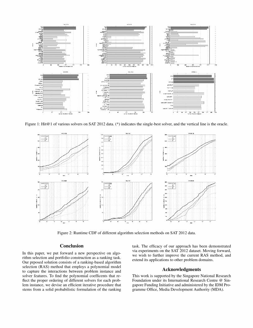
Figure 1: Hit@1 of various solvers on SAT 2012 data. (*) indicates the single-best solver, and the vertical line is the oracle.

Figure 2: Runtime CDF of different algorithm selection methods on SAT 2012 data.

ConclusionIn this paper, we put forward a new perspective on algo-rithm selection and portfolio construction as a ranking task.Our prposed solution consists of a ranking-based algorithmselection (RAS) method that employs a polynomial modelto capture the interactions between problem instance andsolver features. To find the polynomial coefficents that re-flect the proper ordering of different solvers for each prob-lem instance, we devise an efficient iterative procedure thatstems from a solid probabilistic formulation of the ranking

task. The efficacy of our approach has been demonstratedvia experiments on the SAT 2012 dataset. Moving forward,we wish to further improve the current RAS method, andextend its applications to other problem domains.

AcknowledgmentsThis work is supported by the Singapore National ResearchFoundation under its International Research Centre @ Sin-gapore Funding Initiative and administered by the IDM Pro-gramme Office, Media Development Authority (MDA).

ReferencesBaeza-Yates, R. A., and Ribeiro-Neto, B. 1999. Moderninformation retrieval. Boston, MA: Addison-Wesley.Carchrae, T., and Beck, J. C. 2005. Applying machine learn-ing to low-knowledge control of optimization algorithms.Computational Intelligence 21(4):372–387.Cook, S. A. 1971. The complexity of theorem-proving pro-cedures. In Proceedings of the Annual ACM Symposium onTheory of Computing, 151–158.Davey, B. A., and Priestley, H. A. 2002. Introduction tolattices and order. Cambridge University Press.Gagliolo, M., and Schmidhuber, J. 2006. Learning dynamicalgorithm portfolios. Annals of Mathematics and ArtificialIntelligence 47(3-4):295–328.Gomes, C., and Selman, B. 1997. Algorithm portfolio de-sign: Theory vs. practice. In Proceedings of the Conferenceon Uncertainty in Artificial Intelligence, 190–197.Gomes, C. P., and Selman, B. 2001. Algorithm portfolios.Artificial Intelligence 126(1–2):43–62.Guerri, A., and Milano, M. 2004. Learning techniquesfor automatic algorithm portfolio selection. In Proceedingsof the European Conference on Artificial Intelligence, 475–479.Huberman, B. A.; Lukose, R. M.; and Hogg, T. 1997. Aneconomics approach to hard computational problems. Sci-ence 275(5296):51–54.Kadioglu, S.; Malitsky, Y.; Sabharwal, A.; Samulowitz, H.;and Sellmann, M. 2011. Algorithm selection and schedul-ing. In Proceedings of the International Conference on Prin-ciples and Practice of Constraint Programming, 454–469.Leyton-Brown, K.; Nudelman, E.; and Shoham, Y. 2002.Learning the empirical hardness of optimization problems:The case of combinatorial auctions. In Proceedings ofthe International Conference on Principles and Practice ofConstraint Programming, 556–572.Malitsky, Y.; Sabharwal, A.; Samulowitz, H.; and Sellmann,M. 2013. Algorithm portfolios based on cost-sensitive hier-archical clustering. In Proceedings of the International JointConference on Artificial Intelligence, 608–614.Misir, M., and Sebag, M. 2013. Algorithm selection as acollaborative filtering problem. Technical report, INRIA.Nudelman, E.; Devkar, A.; Shoham, Y.; and Leyton-Brown,K. 2004. Understanding random sat: Beyond the clauses-to-variables ratio. In Proceedings of the International Con-ference on Principles and Practice of Constraint Program-ming, 438–452.O’Mahony, E.; Hebrard, E.; Holland, A.; Nugent, C.; andO’Sullivan, B. 2008. Using case-based reasoning in an al-gorithm portfolio for constraint solving. In Proceedings ofthe Irish Conference on Artificial Intelligence and CognitiveScience.Rendle, S.; Freudenthaler, C.; Gantner, Z.; and Schmidt-Thieme, L. 2009. BPR: Bayesian personalized ranking fromimplicit feedback. In Proceedings of the Conference on Un-certainty in Artificial Intelligence, 452–461.

Rice, J. 1976. The algorithm selection problem. Advancesin Computers 15:65–118.Samulowitz, H., and Memisevic, R. 2007. Learning to solveQBF. In Proceedings of the AAAI National Conference onArtificial Intelligence, 255–260.Stern, D.; Herbrich, R.; Graepel, T.; Samulowitz, H.; Pulina,L.; and Tacchella, A. 2010. Collaborative expert portfoliomanagement. In Proceedings of the AAAI National Confer-ence on Artificial Intelligence, 179–184.Stern, D. H.; Herbrich, R.; and Graepel, T. 2009. Matchbox:large scale online bayesian recommendations. In Proceed-ings of the International Conference on World Wide Web,111–120.Streeter, M., and Smith, S. F. 2008. New techniques for al-gorithm portfolio design. In Proceedings of the Conferenceon Uncertainty in Artificial Intelligence, 519–527.Xu, L.; Hutter, F.; Hoos, H.; and Leyton-Brown, K. 2008.SATzilla: portfolio-based algorithm selection for SAT. Jour-nal of Artificial Intelligence Research 32(1):565–606.Xu, L.; Hutter, F.; Hoos, H.; and Leyton-Brown, K. 2012.Evaluating component solver contributions to portfolio-based algorithm selectors. In Proceedings of the Interna-tional Conference on Theory and Applications of Satisfia-bility Testing, 228–241.