Algebraic De Rham Theory for Completions of Fundamental ...
112
Algebraic De Rham Theory for Completions of Fundamental Groups of Moduli Spaces of Elliptic Curves by Ma Luo Department of Mathematics Duke University Date: Approved: Richard Hain, Supervisor Leslie Saper William Pardon Chadmark Schoen Dissertation submitted in partial fulfillment of the requirements for the degree of Doctor of Philosophy in the Department of Mathematics in the Graduate School of Duke University 2018
Transcript of Algebraic De Rham Theory for Completions of Fundamental ...

Algebraic De Rham Theory for Completions ofFundamental Groups of Moduli Spaces of Elliptic
Curves
by
Ma Luo
Department of MathematicsDuke University
Date:Approved:
Richard Hain, Supervisor
Leslie Saper
William Pardon
Chadmark Schoen
Dissertation submitted in partial fulfillment of the requirements for the degree ofDoctor of Philosophy in the Department of Mathematics
in the Graduate School of Duke University2018

Abstract
Algebraic De Rham Theory for Completions of Fundamental
Groups of Moduli Spaces of Elliptic Curves
by
Ma Luo
Department of MathematicsDuke University
Date:Approved:
Richard Hain, Supervisor
Leslie Saper
William Pardon
Chadmark Schoen
An abstract of a dissertation submitted in partial fulfillment of the requirements forthe degree of Doctor of Philosophy in the Department of Mathematics
in the Graduate School of Duke University2018

Copyright c© 2018 by Ma LuoAll rights reserved

Abstract
To study periods of fundamental groups of algebraic varieties, one requires an ex-
plicit algebraic de Rham theory for completions of fundamental groups. This thesis
develops such a theory in two cases. In the first case, we develop an algebraic de
Rham theory for unipotent fundamental groups of once punctured elliptic curves over
a field of characteristic zero using the universal elliptic KZB connection of Calaque-
Enriquez-Etingof and Levin-Racinet. We use it to give an explicit version of Tannaka
duality for unipotent connections over an elliptic curve with a regular singular point
at the identity. In the second case, we develop an algebriac de Rham theory for
relative completion of the fundamental group of the moduli space of elliptic curves
with one marked point. This allows the construction of iterated integrals involving
modular forms of the second kind, whereas previously Brown and Manin only studied
iterated integrals of holomorphic modular forms.
iv

To my parents
v

Contents
Abstract iv
Acknowledgements viii
1 Introduction 1
1.1 Periods . . . . . . . . . . . . . . . . . . . . . . . . . . . . . . . . . . . 1
1.2 Iterated Integrals . . . . . . . . . . . . . . . . . . . . . . . . . . . . . 3
1.3 Algebraic De Rham Theory for Completions of Fundamental Groups 4
1.4 The Genus 0 Case . . . . . . . . . . . . . . . . . . . . . . . . . . . . . 5
1.5 The Elliptic Case . . . . . . . . . . . . . . . . . . . . . . . . . . . . . 6
1.6 The Modular Case . . . . . . . . . . . . . . . . . . . . . . . . . . . . 8
2 Part I: Algebraic De Rham Theory for Unipotent FundamentalGroups of Elliptic Curves 12
2.1 Introduction . . . . . . . . . . . . . . . . . . . . . . . . . . . . . . . . 12
2.2 Moduli Spaces of Elliptic Curves . . . . . . . . . . . . . . . . . . . . . 14
2.3 The Local System H with its Betti and Q-de Rham Realizations . . . 18
2.4 Eisenstein Elliptic Functions and the Jacobi Form F pξ, η, τq . . . . . 22
2.5 Unipotent Completion of a Group and its Lie Algebra . . . . . . . . . 26
2.6 Universal Elliptic KZB Connection—Analytic Formula . . . . . . . . 29
2.7 Elliptic Curves as Algebraic Curves . . . . . . . . . . . . . . . . . . . 31
2.8 Algebraic Connection Formula over E 1 . . . . . . . . . . . . . . . . . 32
2.9 Algebraic Connection Formula over E2 . . . . . . . . . . . . . . . . . 36
vi

2.10 Regular Singularity and Residue at the Identity . . . . . . . . . . . . 39
2.11 Tannaka Theory and a Universal Unipotent Connection over E . . . . 40
2.12 Algebraic Connection Formula over E 1 . . . . . . . . . . . . . . . . . . 49
2.13 Algebraic Connection Formula over E2 . . . . . . . . . . . . . . . . . 54
3 Part II: Algebraic De Rham Theory for the Relative Completion ofSL2pZq 56
3.1 Introduction . . . . . . . . . . . . . . . . . . . . . . . . . . . . . . . . 56
3.2 The Moduli Space M1,1 and Its Open Cover . . . . . . . . . . . . . . 59
3.3 Vector Bundles S2nH onM1,1 and Their Canonical Extensions S2nHon M1,1 . . . . . . . . . . . . . . . . . . . . . . . . . . . . . . . . . . 61
3.4 De Rham Cohomology with Twisted Coefficients . . . . . . . . . . . . 64
3.5 Holomorphic Modular Forms and Modular Forms of the Second Kind 70
3.6 A Q-de Rham Structure on Relative Completion of SL2pZq . . . . . . 79
3.7 Twice Iterated Integrals of Modular Forms . . . . . . . . . . . . . . . 92
4 Conclusion 98
Bibliography 99
Biography 103
vii
Acknowledgements
First, I would like to thank my advisor, Richard Hain, for all his guidance and
encouragement over the years, through his generous support and great inspiration.
He shares his unbounded enthusiasm for mathematics and for life when spending
time with me, which I always appreciate.
I would like to thank Leslie Saper, William Pardon, and Chad Schoen, not only
for serving as my dissertation committee, but also broadening my vision in math-
ematics through discussions. I would also like to thank these committee members
along with my advisor and Paul Aspinwall, Tom Beale, Robert Bryant, Jayce Getz,
Michael Lipnowski, Lenhard Ng, Colleen Robles, David Schaeffer for imparting their
knowledge to me through teaching.
Thanks to Emily Braley, Lewis Blake, Clark Bray, Sarah Schott for providing
constructive advices to develop my teaching skills. Thanks to Andrew Schretter,
Yunliang Yu for the IT supports. Thanks also go to Melissa Blakey, Monique Brown,
Bonnie Farrell, Jenny Hirtz, Tyffany Kittrell, Carolyn Sessoms, Laurie Triggiano,
Wayne Williamson for their genuine help in the math department.
I would like to thank fellow graduate students for academic and nonacademic
activities we enjoyed together: Chen An, Orsola Capovilla-Searle, Ziyu Chen, Yan
Chu, Joshua Cruz, Humberto Diaz, Tingran Gao, Eric Hopper, Xiangying Huang,
Ran Huo, Frank Lee, Wenjing Liao, Didong Li, Lei Li, Yingzhou Li, Weifan Liu,
Ruibo Ma, Shan Shan, Anil Venkatesh, Kangkang Wang, Lihan Wang, Zhe Wang,
viii

Xin Xiong, Chao Xu, Hangjun Xu, Jieren Xu, Rachel Yin, Chi Zhang, Yiyue Zhang.
Special thanks go to Chenjie Fan, Zhangjie Gu, Yuhao Hu, Hangjie Ji, Kevin
Kordek, Yulong Lu, Nils Matthes, Zhao Ni, Yu Pan, Henri Roesch, Yunqing Tang,
Shiqi Wang, Tatsunari Watanabe, Ruixiang Zhang, Yuan Zhang, Zili Zhang, Zhiyong
Zhao, Zhennan Zhou, Wei Zhu, who stood by my side, helped me through difficult
and perplexing times, and set great examples for me to follow over the years.
Thanks to the organizers of the conferences that I attended: Workshop on Fun-
damental Groups and Periods (IAS/Princeton 2014), Moduli Crossroads Retreat
(UW-Madison 2015), AMS Summer Institute in Algebraic Geometry (Utah 2015),
Connecticut Conference on Elliptic Curves, Modular Forms, and Related Topics
(UConn 2016), Triangle Area Graduate Mathematics Conference (UNC 2016, Duke
2017, NCSU 2017), Algebraic Geometry Seminar (Purdue 2017), Hot Topics: Galois
Theory of Periods and Applications (MSRI 2017), Motives for Periods (Freie Uni-
versitat 2017), Periods in Number Theory, Algebraic Geometry and Physics (HIM
2018). Especially the last one, where parts of this thesis are completed.
Finally, I thank my parents for all their support. They have an unwavering belief
in me and provide me with their unconditional love. This thesis is dedicated to them.
ix

1
Introduction
This work is focused on studying periods of fundamental groups of algebraic varieties
defined over Q. To get a theory for periods of fundamental groups, one needs an al-
gebraic de Rham theory for their various completions, such as unipotent completion
and relative (unipotent) completion. Although there are abstract results establishing
the existence of their algebraic de Rham structures [13], one needs concrete construc-
tions and explicit formulas to study the periods. Such explicit constructions were
previously known only for unipotent completions of fundamental groups of hyper-
plane complements. In this thesis, we develop an explicit algebraic de Rham theory
for unipotent completions of fundamental groups of once punctured elliptic curves,
and for the relative completion of the modular group.
1.1 Periods
Periods can be regarded as coefficients of a comparison isomorphism
comp : V dRbQ C «
ÝÑ V BbQ C
1

between the complexifications of two finite dimensional Q-vector spaces: a de Rham
vector space V dRQ and a Betti vector space V B
Q. If γ P V BQ “ HompV B,Qq and
ω P V dRQ , then xcomppωq, γy is a period. Classically, when XQ is a smooth variety
over Q, V dR “ HmdRpXQq is the algebraic de Rham cohomology of X and V B “
HmpXpCq;Qq is the Betti (i.e. singular) cohomology of its corresponding complex
analytic variety XpCq. Grothendieck’s algebraic de Rham theorem provides the
comparison isomorphism, which is induced by integration. If γ P V B and ω P V dR,
then we have
comp : ω ÞÑ pγ ÞÑ
ż
γ
ωq,
and
ż
γ
ω is a period.
Example 1.1.1. Let Gm “ SpecQrx, x´1s. Consider its algebraic de Rham coho-
mology and Betti cohomology:
V dR“ H1
dRpGmq “ Q ¨dx
x
V B“ H1
BpGmpCq;Qq “ Q ¨ σ
where GmpCq “ C˚ denotes the corresponding complex analytic variety, and σ P V B
is the loop wrapping around 0.
0 σ
In this case, Grothendieck’s comparison isomorphism takes dxx
to 2πiσ. The period
is
xcomp
ˆ
dx
x
˙
, σy “
ż
σ
dx
x“ 2πi.
Other interesting examples of periods include elliptic integrals such as
ż 1
0
dxa
xpx´ 1qpx´ tqand
ż 1
0
xdxa
xpx´ 1qpx´ tqwhere t P Q and t ‰ 0, 1,
2

special values of L-functions, and multiple zeta values
ζpn1, ¨ ¨ ¨ , nrq “ÿ
0ăk1㨨¨ăkr
1
kn11 ¨ ¨ ¨ knr
r
where nj ě 1, nr ě 2.
In particular, multiple zeta values can be viewed as periods of fundamental groups
and written as iterated integrals, which we now recall.
1.2 Iterated Integrals
Let X be a complex manifold. Given a path γ : r0, 1s Ñ X and 1-forms ωj on X,
j “ 1, ¨ ¨ ¨ , r, the iterated integral
ż
ω1ω2 ¨ ¨ ¨ωr takes the value
ż
γ
ω1ω2 ¨ ¨ ¨ωr “
ż
0ăt1㨨¨ătră1
f1pt1q ¨ ¨ ¨ frptrqdt1 ¨ ¨ ¨ dtr,
on the path γ, where γ˚ωj “ fjptqdt, j “ 1, ¨ ¨ ¨ , r. If an iterated integral’s value on
a path only depends on its homotopy class relative to end points, then we say this
iterated integral is “closed”. Chen’s π1-de Rham theorem states that
tclosed iterated integrals of smooth 1-forms on Xu«ÝÑ V B
b C,
where
V B“ limÝÑn
HompQπ1pX, xqIn,Qq,
with I being the augmentation ideal of the group algebra Qπ1pX, xq. Note that V B
is a commutative Hopf algebra. The corresponding affine group, defined over Q, is
the unipotent completion of the fundamental group π1pX, xq. We will denote it by
πun1 pX, xq.
When X is a smooth algebraic variety defined over Q, let
V dR“ tclosed iterated integrals of “suitably chosen” algebraic 1-forms on Xu.
3
Then we have a comparison isomorphism
comp : V dRb C «
ÝÑ V Bb C.
Therefore, periods of fundamental groups are given by algebraic iterated integrals.
However, finding the correct set of algebraic iterated integrals is non-trivial, even
when X is a once punctured elliptic curve, as we shall explain in Chapter 2.
Example 1.2.1. Multiple Zeta Values as Iterated Integrals. Let XQ “ P1 ´
t0, 1,8u “ Gm ´ tidu. We have its algebraic de Rham cohomology H1dRpXQq “
Q ¨ ω0 ‘Q ¨ ω1 with basis
ω0 “dx
x, ω1 “
dx
1´ x.
The Q-vector space of periods of the path torsor in X from BBx P T0P1 to ´BBx P
T1P1 is the Q-vector space spanned by multiple zeta values, for example,
ζpnq “
ż 1
0
ω1 ω0 ¨ ¨ ¨ω0
n´ 1
,
and
ζpn,mq “
ż 1
0
ω1 ω0 ¨ ¨ ¨ω0
n´ 1
ω1 ω0 ¨ ¨ ¨ω0
m´ 1
.
1.3 Algebraic De Rham Theory for Completions of Fundamental Groups
Let X be a smooth algebraic variety defined over Q, x P XpQq or a tangential
base point. Denote by π1pX, xq its fundamental group of the corresponding complex
analytic variety. To study its periods, we first linearize π1pX, xq using a suitable
algebraic completion. The Betti incarnation of the completion of π1pX, xq is usually
well known, constructed by group theoretic terms. It is an affine group defined over
Q, which we denote by GB. Its coordinate ring V B “ OpGBq is a Q-vector space.
4

What one needs to find is its de Rham analogue, a Q-group GdRQ , and its coordinate
ring V dR “ OpGdRq. Moreover, there should be a comparison isomorphism
comp : V dRb C «
ÝÑ V Bb C.
We will construct these explicitly when X is a once punctured elliptic curve in
Chapter 2, and the modular curve in Chapter 3.
1.4 The Genus 0 Case
To motivate our results, we first review the genus 0 case. Let X “ P1 ´ t0, 1,8u.
Since fundamental groups depend on its base points, it is natural to consider a vector
bundle
px Ă P
x P X
where the fiber px over x P X is the Lie algebra of the unipotent completion πun1 pX, xq
of the fundamental group π1pX, xq. Since the fundamental group π1pX, xq is a free
group with two generators, px is a (completed) free Lie algebra of rank 2. This is
the Betti side.
Now to the de Rham side. Let Qxxe0, e1yy be the algebra of the formal power
series in noncommuting indeterminants e0, e1, and LQpe0, e1q^ the (completed) free
Lie algebra generated by e0, e1. The 1-form
ωKZ “ ω0e0 ` ω1e1 P H0pΩ1
P1Qplogt0, 1,8uqqbQxxe0, e1yy
defines a flat connection with regular singularities at 0, 1,8 on the trivial bundle
Qxxe0, e1yy ˆ P1Q Ñ P1
Q
5

by the formula ∇f “ df ´ fωKZ . This connection is called the KZ connection. Its
parallel transport function
TKZ : paths in P1´ t0, 1,8uÑ tgroup-like elements of Cxxe0, e1yyu
is given by the formula
γ ÞÑ TKZpγq :“ 1`
ż
γ
ωKZ `
ż
γ
ωKZωKZ `
ż
γ
ωKZωKZωKZ ` ¨ ¨ ¨ .
This induces a comparison isomorphism
comp : Liepπun1 pX, xqq bQ CÑ LQpe0, e1q
^b C
and corresponding comparison isomorphisms for both πun1 pX, xq and its coordinate
ring Opπun1 pX, xqq.
When studying motives unramified over Z, it is necessary to use tangential base
points and regularized periods. For example, one often chooses the tangent vector
´BBx of P1 at x “ 1 and the tangent vector BBx at x “ 0, which we denote by ~v
and ~w respectively. Brown’s work [2] shows that Opπun1 pP1 ´ t0, 1,8u,~vqq generates
the category MTMpZq of mixed Tate motives over Z. Periods of πun1 pP1´t0, 1,8u,~vq,
and thus periods of all objects in MTMpZq, are linear combinations of multiple zeta
values. These multiple zeta values are also the coefficients of the Drinfeld associator
Φpe0, e1q P Cxxe0, e1yy, which is the regularized value of TKZ on the unique straight
line (“dch”) from 0 to 1 (from ~w to ~v to be precise, cf. Example 1.2.1).
1.5 The Elliptic Case
A once punctured elliptic curve E 1 :“ E ´ tidu is given by an affine equation y2 “
4x3´ ux´ v, such that u3´ 27v2 ‰ 0. It is defined over the field K “ Qpu, vq. Then
1-forms dxy
and x dxy
form an K-basis of H1dRpEKq. One can mimic the genus 0 case
6

naively, using the algebraic 1-form
ωnaive “ ´xdx
yT`
dx
yS P H0
pΩ1E1q b LpS,Tq^
to define a flat connection on the trivial bundle LpS,Tq^ ˆ E 1 Ñ E 1. We call this
the naive connection.
Define a regular connection on E to be a meromorphic connection that is holo-
morphic on E 1 and has a regular singularity at the identity. Since the form x dxy
has
a double pole at the identity1, the naive connection is not a regular connection on
E. In fact, this naive connection is not algebraically gauge equivalent to any regular
connection, as we show in Section 2.8.1.
Instead of the naive connection, one should work with the correct elliptic analogue
of the KZ connection, which is called the elliptic KZB connection. As we show in
Section 2.9, if E is an elliptic curve defined over a field K of characteristic 0, then
this connection is defined over K, and has a regular singularity at the identity. In
the analytic setting, this connection was studied by Calaque, Enriquez and Etingof
[5], and by Levin and Racinet [22]. The latter one also provides algebraic formulas
but with irregular singularities at the identity of the elliptic curve E.
The complication is on the bundle that this elliptic KZB connection lives. Deligne’s
canonical extension of this bundle, unlike in the case of P1 ´ t0, 1,8u, is not a triv-
ial bundle as the corresponding monodromy representation fails a Hodge theoretic
restriction (see [16]). One has to trivialize this bundle on an open cover of E. We
choose the cover tE 1, E2u, where E2, containing the identity, is the complement of
three non-trivial 2-torsion points of E (the trivial one being the identity). In Sec-
tions 2.8 and 2.9, we write down algebraic formulas for the elliptic KZB connection
1 Let τ P h, the map z ÞÑ r℘τ pzq, ℘1τ pzq, 1s induces an embedding of the elliptic curve Eτ “ CΛτ
into P2pCq via the Weierstrass ℘-function ℘τ pzq “1z2 ` holo. in z. The pull-back of x dx
y through
this map is ℘τ pzqdz, which has a double pole at z “ 0.
7

explicitly on E 1 and E2. For instance, on E 1, the connection is given by the 1-form
ωKZB “ ´xdx
yT`
dx
yS`
8ÿ
n“2
qnpx, yqdx
yTn ¨ S P H0
pΩ1E1q b LpS,Tq^,
where qnpx, yq are explicit polynomials in Krx, ys that express Eisenstein elliptic
functions in terms of Weierstrass ℘-function and its derivative. While this 1-form
still has a double pole at the identity, we show explicitly that the connection can be
algebraically gauge transformed into a connection that has regular singularity at the
identity on E2. This completes the algebraic de Rham theory in the elliptic case,
and allows one to discuss and study (regularized) periods of πun1 pE
1,~vq, where ~v is a
tangential base point at the identity. We can then define
V dR“ tcoefficients of the transport function TKZBu
where
TKZB “ 1`
ż
ωKZB `
ż
ωKZBωKZB `
ż
ωKZBωKZBωKZB ` ¨ ¨ ¨ .
When K ãÝÑ C, there is a comparison isomorphism
comp : V dRbK C «
ÝÑ V BbQ C,
with V B “ Opπun1 pE
1,~vqq, as required to define periods.
In the spirit of results of Brown [2, 3], when pu, vq P Q2, one can ask whether
Opπun1 pE
1,~vqq generates the conjectural tannakian category MEMpEq of mixed elliptic
motives of EQ.
1.6 The Modular Case
In the modular case, we view SL2pZq as the (orbifold) fundamental group of the
moduli space M1,1 of elliptic curves. Since the unipotent completion of SL2pZq
8

is trivial, we consider instead the relative completion of SL2pZq with respect to
the inclusion SL2pZq ãÝÑ SL2pQq. In fact, the relative completions of SL2pZq and
modular groups are particularly interesting, because they form a bridge between
modular forms and categories of admissible variations of mixed Hodge structures
over modular curves.
More precisely, we regard SL2pZq as the fundamental group π1pM1,1, BBqq, where
the base point BBq is a unit tangent vector at the cusp. The relative completion of
SL2pZq, which we denote by Grel, is an affine group defined over Q. It is an extension
of SL2 by a prounipotent group U rel. The Lie algebra urel of U rel is freely topologically
generated byź
ně0
H1pSL2pZq, S2nHq˚ b S2nH,
where H is the standard representation of SL2, and S2nH its 2n-th symmetric power.
Brown [3] defines multiple modular values to be periods of the coordinate ring
OpGrelq. In order to study and compute multiple modular values, one needs an
explicit Q-de Rham theory for Grel. To do this, the first step is to construct an explicit
Q-de Rham structure on H1pSL2pZq, S2nHq. Recall that there is a mixed Hodge
structure on H1pSL2pZq, S2nHq, which has weight and Hodge filtrations defined over
Q [31]:
W2n`1H1pSL2pZq, S2nHq “ H1
cusppSL2pZq, S2nHq;
W4n`2H1pSL2pZq, S2nHq “ H1
pSL2pZq, S2nHq,
F 2n`1H1pSL2pZq, S2nHq – tholomorphic modular formsu.
The Q-structure for the holomorphic part F 2n`1H1pSL2pZq, S2nHq is classically well-
known; in this holomorphic part, all Q-de Rham classes correspond to classical mod-
ular forms of weight 2n ` 2 with rational Fourier coefficients [15, §21]. To obtain
a complete Q-de Rham basis of H1pSL2pZq, S2nHq, one needs to consider what we
9

call modular forms of the second kind. In Section 3.5.2, we find representatives of all
these Q-de Rham classes in H1pSL2pZq, S2nHq. Our representatives have at worst
logarithmic singularities at the cusp and may have singularities with trivial residue
at other points. This differs from the traditional approach using weakly modular
forms, which allows arbitrary poles at the cusp (cf. Brown–Hain [4]).
Denote the relative completion of π1pM1,1, xq with respect to its inclusion ρx :
π1pM1,1, xq ãÝÑ SL2pQq by Gx. Denote the Lie algebra of its unipotent radical by ux.
They are isomorphic to Grel and urel respectively. We thus have a Betti vector bundle
uB ÑM1,1 whose fiber over x is the Lie algebra ux.
To construct the de Rham analogue udR ÑM1,1, we start from representatives of
all Q-de Rham classes in H1pSL2pZq, S2nHq found earlier. We then apply a Cech-de
Rham version of Chen’s method of power series connections [6] to find a canonical
flat connection, defined over Q and with regular singularity at the cusp, on the vector
bundle udR. This requires us to trivialize udR on the open cover ofM1,1 consisting of
M1,1´trisu andM1,1´trρsu, and to provide an inductive algorithm for constructing
the connection on both opens, and for finding the gauge transformation on their
intersection. We carry this algorithm out explicitly up to udRL3pudRq in Section
3.7.2. This connection is analogous to the KZB connection in the elliptic case §1.5,
but is more general. This enables us to explicitly construct iterated integrals of
algebraic modular forms, involving both holomorphic modular forms and modular
forms of the second kind. This also allows us to define
V dR“ OpGrel
dRq “ t“closed” iterated integrals of algebraic modular formsu,
and a comparison isomorphism
comp : V dRb C «
ÝÑ V Bb C,
with V B “ OpGrelq. These newly constructed iterated integrals provide all multiple
modular values, whereas previously only those multiple modular values that are
10
iterated integrals of holomorphic modular forms have been studied by Brown [3] and
Manin [25, 26].
11

2
Part I: Algebraic De Rham Theory for UnipotentFundamental Groups of Elliptic Curves
2.1 Introduction
A once punctured elliptic curve is an elliptic curve with it identity removed. In this
part, we describe an algebraic de Rham theory for unipotent fundamental groups of
once punctured elliptic curves.
The analytic version of this story is described by Calaque, Enriquez and Etingof
[5] and by Levin and Racinet [22]. For a family X Ñ T where each fiber Xt over
t P T is a once punctured elliptic curve,
Xt Ă X
t P T
there is a vector bundle P of prounipotent groups over X , endowed with a flat
connection. For a point x P X that lies over t, i.e. x P Xt, the fiber of P over x is
the unipotent fundamental group πun1 pXt, xq. We are particularly interested in the
case when X “ E 1 and T “ M1,1. In this case, the flat connection is called the
12

universal elliptic KZB1 connection2. The bundle P extends naturally by Deligne’s
canonical extension P to E , and the universal elliptic KZB connection on P has
regular singularities around boundary divisors: the identity section of the universal
elliptic curve E Ñ M1,1, and the nodal cubic. One can restrict the bundle P to a
single fiber of E 1 ÑM1,1, i.e. a once punctured elliptic curve E 1 :“ E ´ tidu, and
obtain Deligne’s canonical extension P of it to E. It is endowed with a unipotent
connection on E, having regular singularity at the identity. We call this the elliptic
KZB connection on E.
Working algebraically, Levin and Racinet have shown that there is a K-structure
on the bundle P over a punctured elliptic curve X defined over a field K of character-
istic zero, and a Q-structure for the bundle P overM1,2Q. However, their algebraic
formulas for the (universal) elliptic KZB connection is neither explicit nor having
regular singularity at the identity (section). By resolving these issues for the case of
M1,2, we will prove that
Theorem. There is a Q-de Rham structure PdR on the bundle P over M1,2 with
the universal elliptic KZB connection, which has regular singularities along boundary
divisors, the identity section and the nodal cubic.
Restricting to a single elliptic curve, we get
Corollary. If E is an elliptic curve defined over a field K of characteristic zero, then
there is a K-de Rham structure PdR on the bundle P over E with an elliptic KZB
connection, which has regular singularity at the identity.
The tricky part is that Deligne’s canonical extension of PdR, the de Rham realiza-
tion PdR of P , is not a trivial bundle as the corresponding monodromy representation
1 Named after physicists Knizhnik, Zamoldchikov and Bernard.
2 The general universal elliptic KZB connection is the flat connection on the bundle P overM1,n`1
whose fiber over rE; 0, x1, . . . , xns is the unipotent fundamental group of the configuration space ofn points on E1 with base point px1, . . . , xnq. Calaque et al [5] write down the universal elliptic KZBconnection for all n ě 1.
13

fails a Hodge theoretic restriction (see [16]). We trivialize the bundle PdR on two
open subsets of the (universal) elliptic curve, and write down algebraic connection
formulas according to these trivializations, with suitable gauge transformation on
their intersection. These two opens are E 1 and E2, where E2, containing the iden-
tity, is the complement of three non-trivial 2-torsion points of E (the trivial one
being the identity).
For a single elliptic curve EK, this bundle PdR is a universal object of the tan-
nakian category
CdRK :“
$
&
%
unipotent vector bundles V over E defined over Kwith a flat connection ∇ that has regular singularity
at the identity with nilpotent residue
,
.
-
.
This allows us to compute the tannakian fundamental group π1pCdRK , ωq of this cate-
gory, where the fiber functor ω is the fiber over the identity. It is a free pronilpotent
group of rank 2 defined over K. This tannakian formalism implies that the connec-
tion ∇ that we have computed explicitly on the algebraic vector bundle PdR can
be viewed as a universal unipotent connection over EK. Similar results have been
recently obtained by Enriquez–Etingof [12] for the configuration space of n points in
an elliptic curve E with ground field C.
In Section 2.8.1, we show that the naive elliptic analogue of the KZ connection,
which we call the naive connection, cannot be algebraically gauge transformed to
a connection on any Zariski open subset of E that has regular singularity at the
identity. This means the naive connection does not belong to the category CdRK .
2.2 Moduli Spaces of Elliptic Curves
Here we quickly review the construction of moduli spaces of elliptic curves and their
Deligne-Mumford compactifications. Full details can be found in [14], or the first
section of [15].
14

2.2.1 Moduli spaces as algebraic stacks
Denote the moduli stack over Q of elliptic curves with n marked points and r non-
zero tangent vectors by M1,n`~r. Note that M1,n`~r is a scheme if n ą 4 or r ą 0.
The Deligne-Mumford compactification of M1,n will be denoted by M1,n.
One can define M1,n`1 to be the stack quotient of M1,n`~1 by the Gm-action:
λ : rE;x1, ¨ ¨ ¨ , xn;ωs ÞÑ rE;x1, ¨ ¨ ¨ , xn;λωs,
where a moduli point rE;x1, ¨ ¨ ¨ , xn;ωs PM1,n`~1 is represented by tuples
pE;x1, ¨ ¨ ¨ , xn;ωq,
an elliptic curve E with n marked points and the differential form ω that is dual
to the marked tangent vector. For example, the moduli space M1,~1 over Q is the
scheme
M1,~1 :“ A2Q ´D,
where D is the discriminant locus tpu, vq P A2 : ∆ “ u3´27v2 “ 0u. The point pu, vq
corresponds to the once punctured elliptic curve (the plane cubic) y2 “ 4x3´ ux´ v
with the abelian differential dxy. The moduli stackM1,1 is defined as the quotient
of M1,~1 by the Gm-action:
λ ¨ pu, vq “ pλ´4u, λ´6vq.
Its compactification, the moduli stack M1,1, is the quotient of Y :“ A2 ´ tp0, 0qu3
by the same Gm-action above.
Similarly, define the moduli stack M1,2 over Q to be the quotient of the scheme
M1,1`~1 :“ tpx, y, u, vq P A2ˆ A2 : y2
“ 4x3´ ux´ v, and u3
´ 27v2‰ 0u
3 One may regard Y as a partial compactification of M1,~1.
15

by the Gm-action
λ : px, y, u, vq ÞÑ pλ´2x, λ´3y, λ´4u, λ´6vq.
Here the point px, y, u, vq PM1,1`~1 corresponds to the point px, yq on the punctured
elliptic curve y2 “ 4x3 ´ ux ´ v with the abelian differential dxy. Note that M1,2
is E 1, the universal elliptic curve E over M1,1 with its identity section removed. We
define its compactification M1,2 as the quotient of the scheme
tpx, y, u, vq P A2ˆ A2 : y2
“ 4x3´ ux´ v, pu, vq ‰ p0, 0qu
by the same Gm-action above. Note that M1,2 is the compactification E of the
universal elliptic curve E whose restriction to the q-disk is the Tate curve ETate Ñ
SpecZrrqss (see [15, §1]).
2.2.2 Moduli spaces as complex analytic orbifolds
Working complex analytically, we can define moduli spaces as complex orbifolds
Man1,1 :“ GmzzMan
1,~1, Man
1,2 :“ GmzzMan1,1`~1
,
where Man1,~1
:“M1,~1pCq and Man1,1`~1
:“M1,1`~1pCq are complex analytic manifolds.
The moduli space Man1,1 can also be defined as the orbifold quotient SL2pZqzzh of
the upper half plane h by the standard SL2pZq action:
γ “
ˆ
a bc d
˙
: τ ÞÑ γτ “aτ ` b
cτ ` d
where γ P SL2pZq and τ P h. The map
hÑMan1,~1“ tpu, vq P C2 : u3
´ 27v2‰ 0u
τ ÞÑ p20G4pτq,7
3G6pτqq
16

induces an isomorphism of orbifolds SL2pZqzzh – GmzzMan1,~1
, where G2npτq is the
normalized Eisenstein series of weight 2n (see Section 2.4.1 for definition).
A point τ P h corresponds to the framed elliptic curve Eτ :“ CΛτ where Λτ :“
Z‘ Zτ , with a basis a,b of H1pEτ ;Zq that corresponds to 1, τ of the lattice Λτ via
the identification H1pEτ ;Zq – Λτ .
There is a canonical family of elliptic curve Eh over the upper half plane h, called
the universal framed family of elliptic curves in [14], whose fiber over τ P h is Eτ . It
is the quotient of the trivial bundle Cˆ hÑ h by the Z2-action:
pm,nq : pξ, τq ÞÑ
ˆ
ξ ``
m n˘
ˆ
τ1
˙
, τ
˙
.
The universal elliptic curve Ean overMan1,1 is the orbifold quotient of Cˆh by the
semi-direct product4 SL2pZq ˙Z2, where Z2 acts on Cˆ h as above, and γ P SL2pZq
acts as follows:
γ : pξ, τq ÞÑ`
pcτ ` dq´1ξ, γτ˘
.
The universal elliptic curve Ean can also be obtained as the orbifold quotient of Eh Ñ h
by SL2pZq. It is an orbifold family of elliptic curves whose fiber over a moduli point
rEs PM1,1 is an elliptic curve isomorphic to E. If we remove all the lattice points
Λh :“ tpξ, τq P C ˆ h : ξ P Λτu from C ˆ h, then take the orbifold quotient of the
same SL2pZq˙Z2-action above, we obtain another analytic description of the moduli
space Man1,2. To relate the two descriptions, there is a map
Cˆ h´ Λh ÑMan1,1`~1
“ tpx, y, u, vq P C2ˆ C2 : y2
“ 4x3´ ux´ v, pu, vq ‰ p0, 0qu
pξ, τq ÞÑ pP2pξ, τq,´2P3pξ, τq, 20G4pτq,7
3G6pτqq
4 The semi-product structure is induced from the right action of SL2pZq on Z2:
ˆ
a bc d
˙
:
`
m n˘
ÞÑ`
m n˘
ˆ
a bc d
˙
.
17

that induces an isomorphism SL2pZq˙Z2zzpCˆh´Λhq – GmzzMan1,1`~1
, where P2pξ, τq
and P3pξ, τq are, up to a constant, Weierstrass ℘-function ℘τ pξq and its derivative
℘1τ pξq (see Section 2.4.2 for definition).
2.3 The Local System H with its Betti and Q-de Rham Realizations
The local system H over M1,1 is a “motivic local system” R1π˚C associated to the
universal elliptic curve π : E ÑM1,1. It has a set of compatible realizations: Betti,
Q-de Rham, Hodge and l-adic described in [20, §5]. In this section we will follow
[20, §5] closely and describe its Betti realization HB and Q-de Rham realization HdR,
and the comparison between these two.
We will denote the pull back of H (resp. HB, HdR) to M1,n`~r by Hn`~r (resp.
HBn`~r, HdR
n`~r), so that H1 (resp. HB1 , HdR
1 ) is the same as H (resp. HB, HdR).
2.3.1 Betti realization HB
The Betti realization HB of H is the local system R1πan˚ Q over Man
1,1 associated to
the universal elliptic curve πan : Ean Ñ Man1,1. We identify it, via Poincare duality
H1pEq Ñ H1pEq fiberwise, with the local system over Man1,1 whose fiber over rEs P
M1,1 is H1pE;Qq.
There is a natural SL2pZq action
γ “
ˆ
a bc d
˙
:
ˆ
ba
˙
ÞÑ
ˆ
a bc d
˙ˆ
ba
˙
,
where a,b is the basis of H1pEτ ;Zq that corresponds to the basis 1, τ of Λτ . The
sections a,b trivialize the pullback Hh of HB to h.
Denote the dual basis of H1pEτ ;Qq – HompH1pEτ q,Qq by a, b. Then, under
Poincare duality,
a “ ´b and b “ a.
18

And the corresponding SL2pZq-action on this dual basis is
γ :`
a ´b˘
ÞÑ`
a ´b˘
ˆ
a bc d
˙
.
One can construct the local system HB by taking the orbifold quotient of the local
system Hh Ñ h by the above SL2pZq-action.
2.3.2 Q-de Rham realization HdR
The Q-de Rham realization HdR is a vector bundle on M1,1Q. Recall that M1,1 :“
GmzzM1,~1, so to work with M1,1 is to work Gm-equivariantly with M1,~1. Define a
vector bundle
HdR~1
:“ OM1,~1S‘OM1,~1
T
over M1,~1 with a Gm-action:
λ ¨ S “ λ´1S and λ ¨ T “ λT,
where the sections S and T represent algebraic differential forms xdxy and dxy
respectively. This Gm-action extends the action on M1,~1 to the bundle HdR~1
over it.
Define a connection
∇0 “ d`
ˆ
´1
12
d∆
∆T`
3α
2∆S
˙
B
BT`
ˆ
´uα
8∆T`
1
12
d∆
∆S
˙
B
BS, (2.3.1)
where α “ 2udv ´ 3vdu and ∆ “ u3 ´ 27v2 (cf. [15] Prop 19.6). This connection is
Gm-invariant, and defined over Q. Therefore, the bundle HdR~1
with connection ∇0
over M1,~1 descends to a bundle HdR over M1,1.
The canonical extension HdR~1 of HdR
~1to Y :“ A2
Q ´ tp0, 0qu is a vector bundle
HdR~1 :“ OY S‘OYT
19

with the same connection ∇0 above. Since the connection has regular singularities
along the discriminant locus D “ t∆ “ 0u, and recall that M1,1 “ GmzzY from
Section 2.2.1, the bundle HdR~1 Ñ Y descends to a bundle HdR
overM1,1 with regular
singularity at the cusp. It is Deligne’s canonical extension of HdR to M1,1.
2.3.3 The flat vector bundle Han and the comparison between Han and HdR
One can put a complex structure on H. Denote the corresponding holomorphic
vector bundle over Man1,1 by Han. The pullback of Han to h (using the quotient map
hÑMan1,1 “ SL2pZqzzh) is the vector bundle
Hanh “ Oha‘Ohb,
where the sections a and b are flat.
Define a holomorphic section w of Hanh by
wpτq “ wτ “ 2πipa` τ bq “ 2πipτa´ bq,
where wτ is the class in H1pEτ ;Cq represented by the holomorphic differential 2πi dξ.
The sections a and w trivialize the pull back
HanD˚ :“ OD˚a‘OD˚w
of Han to D˚ via the map
hÑ D˚, τ ÞÑ q :“ e2πiτ ,
as they are invariant under τ ÞÑ τ ` 1 (with γ being ˘
ˆ
1 10 1
˙
), and thus invariant
under the monodromy action on the punctured q-disk D˚.
An easy computation [20, §5.2] shows that the connection on HanD˚ in terms of
this framing is
∇an0 “ d` a
B
Bw
dq
q.
20

Since this connection has a regular singularity at the cusp q “ 0, we can extend HanD˚
to the q-disk D by defining
HanD :“ ODa‘ODw.
Therefore, we obtain Deligne’s canonical extension Hanof Han to Man
1,1, endowed
with a connection ∇an0 that has a regular singularity at the cusp.
To relate Betti and de Rham sections of Han, we pull back the bundle Han~1
to h
via the map hÑMan1,~1
in Section 2.2.2, and compare it with Hanh .
Proposition 2.3.1. There is a natural isomorphism
pHan,∇an
0 q – pHdR,∇0q bOM1,1Q
OMan1,1
induced from the pull back. The sections T and S that correspond to dxy and xdxy
respectively, after being pulled back, become T “ w2πi, and S “ pa´2G2pτqwq2πi.
Remark 2.3.2. Our formulas for T and S differ from those in Proposition 5.2 of [20]
by a factor of 2πi. The reason is that the cup product of dxy and xdxy is 2πi, and
we have multiplied their Poincare duals by p2πiq´1 to obtain a Q-de Rham basis of
the first homology [15, §20], such that T “ S and S “ ´T. More explanations are
provided in Section 2.3.4 below.
2.3.4 The fiber of H at the cusp
To better understand various Betti and de Rham sections ofHan, we observe the fiber
H :“ HBBq at the cusp associated to the tangent vector BBq. One can compute the
limit mixed Hodge structure on H (computed in [20, §5.4]), which is isomorphic
to Qp0q ‘ Qp´1q, with Betti realization HB “ Qa ‘ Qb, and de Rham realization
HdR “ Qa‘Qw. Note that on H, ´b “ a “ w2πi spans Qp´1q and a “ b spans
Qp0q.
21

One can think of H as the cohomology H1pEBBqq. It is better to work with first
homology, which is the abelian quotient of the fundamental group. We use Poincare
duality to identify H1pEq with H1pEqp1q. Therefore, we have H1pEBBqq “ Hp1q “
Qp1q ‘ Qp0q, with Betti realization Qa ‘ Qb and de Rham realization QA ‘ QT,
where
A :“ a2πi and T :“ w2πi.
Note that on Hp1q, a “ 2πiA spans Qp1q and ´b “ T spans Qp0q.
By Proposition 2.3.1, we can write S in terms of this de Rham framing A, T of
H (or in fact Hp1q)
S “ A´ 2G2pτqT.
We will use these sections A, S and T to write down the universal elliptic KZB
connection in later sections.
2.4 Eisenstein Elliptic Functions and the Jacobi Form F pξ, η, τq
2.4.1 Eisenstein series
A modular form5 of weight k is a holomorphic function fpτq on the upper half plane
h that satisfies
fpγτq “ pcτ ` dqkfpτq, where γ “
ˆ
a bc d
˙
P SL2pZq , τ P h, and γτ “aτ ` b
cτ ` d.
Since fpτ ` 1q “ fpτq, it has a Fourier expansion of the form
fpτq “ÿ
nPZ
anqn where q “ e2πiτ .
Note that this q-series starting with terms of nonnegative q powers is equivalent to
the condition that a modular form is holomorphic at the cusp. Moreover, a modular
form is called a cusp form if the leading coefficient a0 of its q-series is 0.
5 In this paper, we will only consider modular forms of level one, i.e. those with respect to theentire modular group SL2pZq.
22

Example 2.4.1. Weight k Eisenstein Series ek. For τ P h, define
ekpτq :“ÿ
n,mpn,mq‰p0,0q
pnτ `mq´k.
Note that ek “ 0 if k is odd.
Example 2.4.2. Normalized Weight k Eisenstein Series Gk. We will normalize
the Eisenstein series following Zagier [30]. Define Gk to be zero when k is odd. For
k ě 1, G2kpτq :“ 12p2k´1q!p2πiq2k
e2kpτq, it has Fourier expansion
G2kpτq “ ´B2k
4k`
8ÿ
n“1
σ2k´1pnqqn
where Bk’s are Bernoulli numbers6 and σkpnq “ř
d|n dk, with
G2k|q“0 “ ´B2k
4k“p2k ´ 1q!
p2πiq2kζp2kq.
When k ą 2 is even, the series for Gk is absolutely convergent. It is holomorphic
on the upper half plane, satisfying Gkpγτq “ pcτ ` dqkGkpτq, and it is holomorphic
at the cusp. Therefore, it is a modular form of weight k. When k “ 2, the series
needs to be added in some specific order (cf. [29]), and it satisfies (cf. [30])
G2pγτq “ pcτ ` dq2G2pτq ` icpcτ ` dq4π.
It is well known that the ring of all normalized (Hecke eigen) modular forms is
the polynomial ring QrG4, G6s.
2.4.2 Eisenstein elliptic functions
For k ě 2, τ P h and ξ P C, define Eisenstein elliptic functions [29] by
Ekpξ, τq :“ÿ
n,m
pξ ` nτ `mq´k.
6 One can define Bernoulli numbers Bn by xex´1 “
ř8
n“0Bnxn
n! . Note that B0 “ 1, B1 “ ´12and that B2k`1 “ 0 when k ą 0.
23

We will need the following formula, which is adapted from equation (9) of Chap. IV
in [29].
Formula 2.4.3.
2πiBE1
Bτ“ E3 ´ E1E2.
Now we define functions Pkpξ, τq for k ě 2
Pkpξ, τq :“ p2πiq´kpEkpξ, τq ´ ekpτqq.
Note that up to a scalar, P2 and P3 are the Weierstrass ℘-function ℘τ pξq and its
derivative respectively.
These Pk’s satisfy recurrence relations (cf. [29]): for m ě 3, n ě 3,
PmPn ´ Pm`n “p´1qn
pn´ 1q!
m´2ÿ
h“1
2
h!Gn`hPm´h
`p´1qm
pm´ 1q!
n´2ÿ
k“1
2
k!Gm`kPn´k
` p´1qm2pm` nq
m!n!Gm`n
The same relation also holds for m “ 2, n ě 2.
Therefore, the algebra generated by Eisenstein elliptic functions is the ring KrP2, P3s
with coefficients in K :“ QrG4, G6s.
Remark 2.4.4. If variable τ is fixed, one can use P2, P3 to embed the elliptic curve Eτ
into a cubic in P2 (see Section 2.7), then Pk’s are algebraic functions on this elliptic
curve. In particular, if the elliptic curve Eτ is defined over a field K of characteristic
0, then there is an embedding with G4, G6 P K, so that Gk P K for all k ě 4.
Therefore, Pk’s are polynomials of P2, P3 with coefficients in K, i.e. Pk’s are in the
coordinate ring OpEτKq, which is a K-algebra generated by P2, P3.
24

2.4.3 The Jacobi forms F pξ, η, τq and F Zagpu, v, τq
There are two different versions of the Jacobi form F : one F pξ, η, τq used by Levin–
Racinet [22], and another F Zagpu, v, τq used by Zagier [30]. They are related to each
other by
F pξ, η, τq “ 2πiF Zagp2πiξ, 2πiη, τq.
In this paper, we will use F Zag exclusively.
2.4.4 Some useful formulas
In this section, we provide some formulas that will be used in later sections.
First, we express the Jacobi form F Zag in terms of Eisenstein elliptic functions
Pk “ p2πiq´kpEk ´ ekq for k ě 2 and p2πiq´1pE1 ´ e1q “ p2πiq
´1E1.
Formula 2.4.5.
TF Zagp2πiξ, T, τq “ exp
´
´
8ÿ
k“1
p´T qk
kPkpξ, τq
¯
.
Proof. By [30] p456, (viii),
F Zagpu, v, τq “
u` v
uvexp
´
ÿ
ką0
2
k!ruk ` vk ´ pu` vqksGkpτq
¯
.
Multiplying v, then take logarithm on both sides, we get
logpvF Zagpu, v, τqq “ logp1`
v
uq `
ÿ
ką0
2
k!ruk ` vk ´ pu` vqksGkpτq
“ ´
8ÿ
k“1
p´vuqk
k`
8ÿ
k“1
2vk
k!r1` p
u
vqk´ p1`
u
vqksGkpτq
25

Let u “ 2πiξ, v “ T , and rescale Gk back to ek, we have
logpTF Zagp2πiξ, T, τqq
“ ´
8ÿ
k“1
p´T 2πiξqk
k`
8ÿ
k“1
2T k
k!
„
1` p2πiξ
Tqk´ p1`
2πiξ
Tqk
1
2
pk ´ 1q!
p2πiqkekpτq
“ ´
8ÿ
k“1
p´T qk
kp2πiξq´k ´
8ÿ
l“1
T l
lp2πiq´l
l´1ÿ
k“1
ˆ
l
k
˙
p2πiξ
Tql´kelpτq
“ ´
8ÿ
k“1
p´T qk
kp2πiq´k
1
ξk´
8ÿ
k“1
T k
kp2πiq´k
8ÿ
l“k`1
k
l
ˆ
l
k
˙
ξl´kelpτq
“ ´
8ÿ
k“1
p´T qk
kp2πiq´k
1
ξk´
8ÿ
k“1
p´T qk
kp2πiq´kp´1qk
8ÿ
l“k`1
ˆ
l ´ 1
k ´ 1
˙
ξl´kelpτq
“ ´
8ÿ
k“1
p´T qk
kp2πiq´k
«
1
ξk` p´1qk
8ÿ
l“k`1
ˆ
l ´ 1
k ´ 1
˙
ξl´kelpτq
ff
“ ´
8ÿ
k“1
p´T qk
kp2πiq´kpEk ´ ekq “ ´
8ÿ
k“1
p´T qk
kPkpξ, τq
where the last line follows from equation (10) of Chap. III in [29], and the facts that`
l´1k´1
˘
“ 0 for l ă k and that ekpτq “ 0 for odd k. After taking exponential on both
sides, (2.4.5) follows.
Taking partial derivative with respect to T , we have
Formula 2.4.6.
TBF Zag
BTp2πiξ, T, τq “ exp
´
´
8ÿ
k“1
p´T qk
kPkpξ, τq
¯´
8ÿ
k“1
p´T qk´1Pkpξ, τq ´1
T
¯
.
2.5 Unipotent Completion of a Group and its Lie Algebra
Given a finitely generated group Γ, and a field K of characteristic 0. The group
algebra KΓ is naturally a Hopf algebra with coproduct, antipode and augmentation
26

given by
∆ : g ÞÑ g b g, i : g ÞÑ g´1, ε : g ÞÑ 1.
Note that it is cocommutative but not necessarily commutative, and thus not corre-
sponding to the coordinate ring of an (pro-)algebraic group. It is natural to consider
its (continuous) dual, which is commutative. We define the unipotent completion
Γun of Γ over K, an (pro-)algebraic group, by its coordinate ring
OpΓunKq “ HomctspKΓ,Kq :“ lim
ÝÑn
HompKΓIn,Kq,
where we give KΓ a topology by powers of its augmentation ideal I :“ ker ε. The set
of its K-rational points ΓunpKq is in 1-1 correspondence with the set of
tring homomorphisms OpΓunKq Ñ Ku.
For example, any γ P Γ gives a ring homomorphism OpΓunKq Ñ K by evaluating
OpΓunKq at γ, thus determines a K-point γ P ΓunpKq.
For the purpose of this paper, we only need to consider the case of Γ being a free
group.
2.5.1 The unipotent completion of a free group
Suppose that Γ is the free group xx1, . . . , xny generated by the set tx1, . . . , xnu. The
coordinate ring OpΓunq of its unipotent completion Γun over K is a K vector space
spanned by a basis taIu indexed by tuples I “ pi1, i2, ¨ ¨ ¨ , irq, where ij P t1, 2, ¨ ¨ ¨ , nu.
If the index is empty, then a∅ ” 1; if the index tuple only consists of one number
I “ piq, we will simply write aI as ai. The product structure on OpΓunq is induced
by shuffle product x and linearity
aI ¨ aJ “ÿ
KP Ix J
aK .
27

For each K-point γ P ΓunpKq, “coordinate function” aI takes value aIpγq in K, and
aIpγq ¨ aJpγq “ÿ
KP Ix J
aKpγq. (2.5.1)
Note that it is natural to define ta1, ¨ ¨ ¨ , anu as the dual basis of tx1, ¨ ¨ ¨ , xnu, so
that aipxjq “ δij.
To determine the structure of Γun, consider the ring KxxX1, . . . , Xnyy of formal
power series in the non-commuting indeterminants Xj. It is a Hopf algebra with each
Xj being primitive, and its augmentation ideal is the maximal ideal I “ pX1, . . . , Xnq.
There is a unique group homomorphism
θ : Γ Ñ KxxX1, . . . , Xnyy
γ ÞÑÿ
I
aIpγqXI
that takes xj to exppXjq, where for I “ pi1, i2, ¨ ¨ ¨ , irq, define XI :“ Xi1Xi2 ¨ ¨ ¨Xir .
For any K-point γ P ΓunpKq, the elementř
I aIpγqXI is group-like by (2.5.1).
This induces a continuous isomorphism
θ : ΓunpKq Ñ tgroup-like elements in KxxX1, . . . , Xnyy
^u,
where KxxX1, . . . , Xnyy^ is completed from KxxX1, . . . , Xnyy with respect to its aug-
mentation ideal.
It is easy to use universal mapping properties to prove:
Proposition 2.5.1. The homomorphism θ is an isomorphism of complete Hopf al-
gebras.
Corollary 2.5.2. The restriction of θ induces a natural isomorphism
dθ : LiepΓunpKqq Ñ LKpX1, . . . , Xnq
^
of topological Lie algebras.
28

Proof. This follows immediately from the fact that θ induces an isomorphism on
primitive elements and the well-known fact that the set of primitive elements of the
power series algebra KxxX1, . . . , Xnyy is the completed free Lie algebra LKpX1, . . . , Xnq^.
Remark 2.5.3. By the Baker-Campbell-Hausdorff formula, the exponential map
exp : LKpX1, . . . , Xnq^Ñ tgroup-like elements in KxxX1, . . . , Xnyy
^u,
is a group isomorphism. Therefore, ΓunpKq and its Lie algebra LiepΓunpKqq are
isomorphic as groups.
2.6 Universal Elliptic KZB Connection—Analytic Formula
In this section, we describe the main object to be studied in this paper. There is a
canonical vector bundle P (resp. p) overM1,2 whose fiber over a moduli point rE 1, xs
is the unipotent fundamental group πun1 pE
1, xq (resp. Liepπun1 pE
1, xqq).7 This vector
bundle comes with an integrable connection, which is called the universal elliptic
KZB connection. Analytic formulas for this connection have been given in different
forms by Levin and Racinet [22] and by Calaque, Enriquez and Etingof [5].
The universal elliptic KZB connection for the bundle P over E 1 actually lives on
E , even E . Since P is a unipotent vector bundle, using Deligne’s canonical extension,
we obtain P over E by extending P across the boundary divisors, the identity section
and the nodal cubic. The universal elliptic KZB connection has regular singularities
around these divisors, as is shown in [15, §12, §13].
By Section 2.5.1, the fiber of P over a point rE 1, xs is the Lie algebra Liepπun1 pE
1, xqq
of its unipotent fundamental group πun1 pE
1, xq, which can be identified with LCpA,Tq^,
where A and T are the sections defined in §2.3.4.
7 From Remark 2.5.3, the unipotent completion of a group and its Lie algebra are isomorphic, wewill regard this bundle as a local system of both unipotent fundamental groups and Lie algebras,whichever is appropriate.
29

We now write the connection form in terms of analytic coordinates pξ, τq on Cˆh.
It is shown to be SL2pZq ˙ Z2-invariant and flat in [15, §9]. Therefore, it descends
to a flat connection on the bundle P over the orbifold E .
The connection is defined by
∇anf “ df ` ωf,
with a 1-form
ω P Ω1pCˆ h log Λhq bDerLCpA,Tq
^,
whose analytic formula is given by
ω “ 2πi dτ b AB
BT` ψ ` ν,
with
ψ “ÿ
mě1
G2m`2pτq
p2mq!2πi dτ b
ÿ
j`k“2m`1j,ką0
p´1qjradjTpAq, adkTpAqsB
BA,
and
ν “ ν1 ` ν2 “ TF Zagp2πiξ,T, τq ¨ Ab 2πi dξ ` p
1
T`T
BF Zag
BTp2πiξ,T, τqq ¨ Ab 2πi dτ.
Here, we view LCpA,Tq^ as a Lie subalgebra of DerLCpA,Tq
^ via the adjoint action,
and Tn acts on LCpA,Tq^ as adnT.
In this part, we describe an algebraic de Rham structure PdR on the restriction
of the canonical bundle P to a single elliptic curve E. We essentially reproduce and
then complete the unfinished work of Levin–Racinet [22, §5]. In particular, their
connection, though being algebraic, has an irregular singularity at the identity of the
elliptic curve. Moreover, their formula is not explicit.
We compute explicitly the restriction of the universal elliptic KZB connection
to a single elliptic curve in terms of its algebraic coordinates. We resolve the issue
30

of irregular singularities at the identity in the connection formula by trivializing
the bundle PdR on two open subsets of E, one of which contains a neighborhood
of the identity where the connection has a regular singularity. Therefore, we have
constructed a de Rham structure PdR on P over E. Trivializing it on different open
subsets is necessary because Deligne’s canonical extension P of P from E 1 (elliptic
curve E punctured at the identity) to E, unlike the genus zero case (of P1), is not
trivial as an algebraic vector bundle.
2.7 Elliptic Curves as Algebraic Curves
Fix τ P h and an elliptic curve E “ Eτ . Using the Weierstrass ℘-function
℘τ pξq :“ E2pξ, τq ´ e2pτq,
we can embed a punctured elliptic curve E 1 into P2 as follows:
ξ ÞÑ rp2πiq´2℘τ pξq, p2πiq´3℘1τ pξq, 1s.
8
This satisfies an affine equation
y2“ 4x3
´ ux´ v,
where u “ g2pτq “ 20G4pτq, v “ g3pτq “73G6pτq. It is defined over K :“ Qpu, vq.
The identity of E is at the infinity. The equation y “ 0 picks out three nontrivial
order 2 elements in E (the trivial one being the identity), we define
E2 :“ E ´ ty “ 0u.
Note that id P E2, and tE 1, E2u form an open cover of E.
By pulling back through the above embedding, one can identify algebraic func-
tions and forms with their analytic counterparts, which is how we will turn the
8 We choose this embedding so that powers of 2πi will not appear in our algebra formulas of KZBconnections later.
31

analytic formula of the connection into an algebraic formula. For example, coordi-
nate functions x,´y2
pull back to P2, P3 defined in Section 2.4.2, and the differential
dxy
pulls back to 2πi dξ. Note from Remark 3.6.1 that for k ě 2, Pk can be expressed
by a polynomial of P2, P3, i.e. Pk “ Pkpx, yq P Krx, ys.
2.8 Algebraic Connection Formula over E 1
Fix τ P h, an elliptic curve E “ Eτ defined over a field K of characteristic zero, and
its algebraic embedding as in the last section. The elliptic KZB connection restricted
from the universal one to the once punctured elliptic curve E 1 “ E ´ tidu is
∇an“ d` ν1 “ d` TF Zag
p2πiξ,T, τq ¨ Ab 2πi dξ. (2.8.1)
Note that when described in terms of sections A and T, the bundle P has factors
of automorphy [15, §6]. We would like to make sections of P elliptic (i.e. periodic
with respect to the lattice Λτ ) by a gauge transformation so that the connection
form would also be elliptic and can be expressed in terms of algebraic coordinate
functions x, y, and Pk’s. Following Levin–Racinet [22, §5] and using Formula 2.4.5,
the connection tranforms under the gauge galgpξq “ expp´ 12πiE1Tq into ∇ “ d` νalg
1 ,
with 1-form
νalg1 “ ´dgalg ¨ g
´1alg ` galg ν1 g
´1alg
“ ´1
2πiE2T dξ ` exp
´
´E1
2πiT¯
exp´
´
8ÿ
k“1
p´Tqk
kPkpξ, τq
¯
¨ Ab 2πi dξ
“ ´p2πiq´2pE2 ´ e2qTb 2πidξ
` exp´
´
8ÿ
k“2
p´Tqk
kPkpξ, τq
¯
¨ pA´ p2πiq´2e2Tq b 2πi dξ
32

“ ´xdx
yT` exp
´
´
8ÿ
k“2
p´Tqk
kPkpx, yq
¯
¨ Sb 2πi dξ
“ ´xdx
yT`
dx
yS`
8ÿ
n“2
qnpx, yqdx
yTn ¨ S.
Here νalg1 P Ω1pE 1
Kq b LKpS,Tq^ and
qnpx, yq “ÿ
2a2`3a3`¨¨¨`nan“n
1
a2!a3! ¨ ¨ ¨ an!
nź
k“2
ˆ
p´1qk`1Pkpx, yq
k
˙ak
P OpE 1Kq,
where OpE 1Kq “ Krx, yspy2 ´ 4x3 ` ux ` vq. Note that the above sum is indexed
by the partitions of integer n with summands at least 2. For example, 5 has 2 such
partitions: 5 and 2` 3, so q5 “P5
5` p´P2
2q ¨ P3
3“ 1
5P5 ´
16P2P3.
Remark 2.8.1. One can use the recurrence relations of Pk’s described in Section 2.4.2
to find relations among qn’s.
Note that the form νalg1 is defined over K, so we have constructed an algebraic
vector bundle pPdR,∇q over E 1 whose fibers can be identified with LKpS,Tq^. This
algebraic bundle is defined over K, with its connection ∇ also defined over K. It
provides us with a K-structure PdR on P over E 1. Since the form νalg1 has irregular
singularity (xdxy
having a double pole) at the identity, we cannot extend it naively
across the identity to obtain Deligne’s canonical extension. To construct the canon-
ical extension, we have to change gauge on a Zariski open neighborhood E2 of the
identity. We do this in Section 2.9.
2.8.1 The naive connection vs. the elliptic KZB connection
Before we do this, we consider the naive connection on the trivial bundle
LKpS,Tq^ˆ E 1 Ñ E 1
33

which is defined by ∇1 “ d` νnaive1 , where
νnaive1 “ ´
xdx
yT`
dx
yS.9
This flat connection is defined over K, whose monodromy also induces an isomor-
phism between Lieπun1 pE
1, xqbKC and LCpS,Tq^. Since the elliptic KZB connection
∇ “ d ` νalg1 induces the same isomorphism (up to an inner automorphism of the
fiber), one might expect that it gives the same K-structure as the naive connection.
However, this is not the case. The first step is the following lemma.
Lemma 2.8.2. Fix a field K of characteristic zero. The elliptic KZB connection
∇ “ d ` νalg1 and the naive connection ∇1 “ d ` νnaive
1 are not algebraically gauge
equivalent over any Zariski open subset of EK.
Proof. Suppose they were gauge equivalent, there would be a gauge transformation
g : E expLpS,Tq^ Ă AutLpS,Tq^, with coefficients in KpEq, field of fractions of
OpE 1Kq, such that
νalg1 “ ´dg ¨ g´1
` gνnaive1 g´1,
or equivalently
dg “ gνnaive1 ´ νalg
1 g. (2.8.2)
This is an equation of 1-forms on E with values in DerLpS,Tq^. Identify DerLpS,Tq^
with the universal enveloping algebra of LpS,Tq^, and let
g “ 1` αT`βS` γT2` λST` µTS` δS2
` σT3` ζT2S` ηTST` ξTS2
` τST2` κSTS` εS2T` ιS3
` ¨ ¨ ¨
where coefficients α, β, γ, ¨ ¨ ¨ P KpEq should be regarded as rational functions on the
elliptic curve EK. We substitute g into the above equation (3.6.2). Now we equate
9 The “´”-sign appears as we regard ´T and S as a basis for H1pEq, dual to S “ xdxy andT “ dxy in H1pEq, see Remark 2.3.2 before Section 2.3.4.
34

the coefficients up to the third degree of derivations in DerLpS,Tq^. We have
dα “ 0, dβ “ 0, dγ “ 0, dδ “ 0, dσ “ 0 (2.8.3)
dµ “ αdx
y` β
x dx
y(2.8.4)
dλ “ ´βx dx
y´ α
dx
y(2.8.5)
dζ “ γdx
y` µ
x dx
y`
1
2
x dx
y(2.8.6)
dη “ ´µx dx
y` λ
x dx
y(2.8.7)
dξ “ µdx
y` δ
x dx
y(2.8.8)
¨ ¨ ¨ (2.8.9)
From (2.8.3), we know that α and β are constants. Taking cohomology classes on
both sides of (2.8.4), we have α rdxys ` β rx dx
ys “ 0, and easily get α “ β “ 0. Thus
dµ “ 0, and µ is a constant. For the same reason, λ is a constant.
Now taking cohomology classes on both sides of (2.8.6) and of (2.8.7), we get
γ “ 0, and λ “ µ “ ´12. Similarly, taking cohomology classes on both sides of
(2.8.8), we get µ “ δ “ 0. However, µ cannot be ´12
and 0 at the same time!
Proposition 2.8.3. The naive connection provides a different K-structure than the
canonical K-structure given by the elliptic KZB connection.
Proof. Note that the elliptic KZB connection has regular singularity at the identity
(already known analytically and will be shown algebraically in the next two sections).
Suppose the K-structures on the vector bundles over E 1 given by both connections
were the same, then their canonical extensions a la Deligne from E 1 to E would be
the same up to a gauge transformation. In particular, working over C, there would
be a morphism between their sheaves of flat sections of these vector bundles over
35

E, which is compatible with the connections and meromorphic at the identity. This
contradicts Lemma 2.8.2 when the field is C.
Remark 2.8.4. Since the monodromy representations induced by both connections are
the same (up to conjugacy) over C, there is a complex analytic gauge transformation
between the connections. Our discussion above in the proof shows that this complex
analytic gauge transformation cannot be meromorphic at the identity, so it must
have an essential singularity there.
Remark 2.8.5. Working over C, define a regular connection over E to be a mero-
morphic connection over E that is holomorphic on E 1 and has at most a simple pole
at the identity under some meromorphic gauge transformation. It follows from the
previous lemma that the naive connection is not a regular connection. Otherwise,
by Riemann-Hilbert correspondence,
"
local systemsV over E 1
*
Ø
$
&
%
vector bundles Vover E 1 with a flat
connection ∇
,
.
-
Ø
$
&
%
vector bundles Vover E with a regular
connection ∇
,
.
-
,
the naive connection and the elliptic KZB connection over E 1, having the same mon-
odromy representation up to conjugacy, would extend to the same regular connection
over E up to gauge equivalence, which contradicts the lemma.
2.9 Algebraic Connection Formula over E2
Recall that we have an analytic local system pP ,∇anq of (Lie algebras of) unipo-
tent fundamental groups over E 1. The elliptic KZB connection ∇an is obtained by
restricting the universal elliptic KZB connection to E 1. Note that the analytic for-
mula of the elliptic KZB connection ∇an has regular singularity at the identity with
pronilpotent residue. The elliptic KZB connection thus extends naturally from E 1 to
E, and we obtain Deligne’s canonical extension pP ,∇anq of pP ,∇anq. It is not imme-
36

diately clear that pP ,∇anq has an algebraic de Rham structure. The question is to
determine whether this canonical extension is defined over K, the field of definition of
E. In this section, we show that the elliptic KZB connection ∇an is gauge equivalent
to its algebraic counterpart ∇ defined over K, which has regular singularity at the
identity with pronilpotent residue. It follows that Deligne’s canonical extension P
of P to E is defined over K.
We start with the algebraic connection ∇ “ d`νalg1 , which is defined to be gauge
equivalent to the analytic one ∇an in the last section. Since νalg1 has irregular sin-
gularities at the identity of E, we would like to apply another gauge transformation
to make it regular. The reason νalg1 has irregular singularity is that we introduced
a gauge transformation involving E1, which has a pole at the identity. To cancel
this effect and make the connection regular at the identity, we apply a gauge trans-
formation greg “ expp´2x2
yTq. Then the connection becomes ∇ “ d ` νreg
1 , with
1-form
νreg1 “ ´dgreg ¨ g
´1reg ` greg ν
alg1 g´1
reg
“
ˆ
d
ˆ
2x2
y
˙
´xdx
y
˙
T` exp´
´2x2
yT´
8ÿ
k“2
p´Tqk
kPkpx, yq
¯
¨ Sb 2πi dξ
“
ˆ
d
ˆ
2x2
y
˙
´xdx
y
˙
T`dx
yS`
8ÿ
n“1
rnpx, yqdx
yTn ¨ S.
Here νreg1 P Ω1pE2 logtiduq b LKpS,Tq
^ and we have rational functions
rnpx, yq “ÿ
a1`2a2`3a3`¨¨¨`nan“n
1
a1!a2!a3! ¨ ¨ ¨ an!
nź
k“1
ˆ
p´1qk`1Pkpx, yq
k
˙ak
P OpE2´tiduq,
where P1px, yq :“ ´2x2
yand OpE2´tiduq “ OpE 1yq “ OpE 1qry´1s. Note that the sum
for rn is indexed by the partitions of integer n with no restrictions of the summands.
37
For example, 4 has 5 partitions: 4, 3` 1, 2` 2, 2` 1` 1, 1` 1` 1` 1, so
r4 “ p´P4
4q `
1
1!1!pP3
3q ¨ p
P1
1q `
1
2!p´P2
2q2`
1
2!1!pP1
1q2¨ p´
P2
2q `
1
4!pP1
1q4
“ ´1
4P4 `
1
3P3P1 `
1
8P 2
2 ´1
4P2P
21 `
1
24P 4
1
Remark 2.9.1. One can use the recurrence relations of Pk’s described in Section 2.4.2
to find relations among rn’s.
In the next section, we will check that
Lemma 2.9.2. The connection ∇ “ d`νreg1 has a regular singularity at the identity
with pronilpotent residue.
Therefore, this connection a priori living on E2´tidu, can be extended naturally
across the identity. It is an algebraic connection defined over K on an algebraic vector
bundle PdR|E2 over the open subset E2 of E. This is one part of a vector bundle
PdR over E. The other part PdR|E1 “ PdR was constructed using the connection
∇ “ d ` νalg1 in the last section. Now we have trivialized PdR on an open cover of
two different subsets of E. By gluing two trivializations together in terms of the
gauge transformation, we have constructed an algebraic vector bundle PdR over E.
Summarizing results in this part, we get
Theorem 2.9.3 (The algebraic de Rham structure PdR on P over E). Suppose
that K is a field of characteristic 0, embeddable in C. Let E be an elliptic curve
defined over K. Then for each embedding σ : K ãÝÑ C, we have an algebraic vector
bundle PdR over EK endowed with connection ∇, and an isomorphism
pPdR,∇q bK,σ C « pP ,∇anq.
The algebraic bundle PdR and its connection ∇ are both defined over K. The K-de
Rham structure pPdR,∇q on pP ,∇anq is explicitly given by the connection formulas
38

for νalg1 on E 1 and νreg
1 on E2 above. In particular, the connection ∇ has a regular
singularity at the identity.
2.10 Regular Singularity and Residue at the Identity
In this section, we prove Lemma 2.9.2 by showing that νreg1 has regular singularity
at the identity, and we compute its residue there.
It is easy to check that analytically d´
2x2
y
¯
´ xdxy
is holomorphic at the identity.
So we are left to check that
1`8ÿ
n“1
rnpx, yqTn“ exp
´
´
8ÿ
k“1
p´Tqk
kPkpx, yq
¯
(2.10.1)
has a regular singularity at the identity.
Let ξ be the complex coordinate near the identity. Analytically, we need to
calculate (in terms of ξ) the principal parts of P1 “ ´2x2
yand Pk’s pk ě 2q. The
principal part of P1 “ ´2x2
yis 1
2πiξ; the principal part of Pk pk ě 2q is 1
p2πiξqk, since
Pk “ p2πiq´kpEk ´ ekq
“ p2πiq´kÿ
m,n
pξ `mτ ` nq´k ´ÿ
m,n
1
pmτ ` nq´k
“1
p2πiqkξk` p2πiq´k
ÿ
m,n
1ˆ
1
pξ `mτ ` nqk´
1
pmτ ` nqk
˙
“1
p2πiqkξk` p2πiq´k
ÿ
m,n
1 1
pmτ ` nqk
8ÿ
l“1
p´1qlˆ
l ` k ´ 1
k ´ 1
˙
ξl
pmτ ` nql
“1
p2πiξqk`
8ÿ
l“1
p´1qlˆ
l ` k ´ 1
k ´ 1
˙
p2πiq´pk`lqek`l p2πiξql.
39

Therefore, (2.10.1) is of the following form near ξ “ 0,
exp´
´
8ÿ
k“1
p´Tp2πiξqqk
k` holo. in ξ
¯
“ exp plnp1` Tp2πiξqqq exp´
8ÿ
n“0
anpTqp2πiξqn¯
“ p1` Tp2πiξqq exp´
8ÿ
n“1
anpTqp2πiξqn¯
,
which has a regular singularity at the identity. Here @n ě 0, anpTq P KrTs and
a0pTq “ 0.
Now it’s easy to calculate the residue. Note that 2x2
yis an odd function in ξ, and
when expressed in terms of ξ, it has constant term 0 in the holomorphic part; so
does each of the Pk’s according to their expansions above. Therefore, we know that
the holomorphic part in ξ also has constant term 0, and the residue at the identity
we are looking for is then
T
2πiexpp0q ¨ Sp2πiq “ T ¨ S “ adrT,Ss,
which is pronilpotent in DerLpS,Tq^. Note that p2πiq at the end of the first expres-
sion above comes from dxy “ 2πidξ.
2.11 Tannaka Theory and a Universal Unipotent Connection over E
Recall that a unipotent object in a tensor category C with the identity object 1C is
an object V with a filtration in C
0 “ V0 Ď ¨ ¨ ¨ Ď Vn “ V
such that each quotient VjVj´1 is isomorphic to 1‘kjC for some kj P N.
Let E be an elliptic curve defined over K and E 1 “ E ´ tidu. Consider the
following tensor categories:
40

1. Unipotent Local Systems
CBF :“ tunipotent local systems VF over E 1pCqu,
where F is a field of characteristic 0, and the identity object 1CBF
is the constant
sheaf FE1 on E 1pCq;
2. Algebraic de Rham
CdRK :“
$
&
%
unipotent vector bundles V over EK defined over Kwith a flat connection ∇ that has regular singularity
at the identity with nilpotent residue
,
.
-
,
where the identiy object 1CdRK
is the trivial vector bundle OE with the trivial
connection given by the exterior differential d;
3. Analytic de Rham
Can :“
$
&
%
unipotent flat vector bundles Vanover Ean with a connection
that is holomorphic over E 1pCq, meromorphic over EpCq andhas regular singularity at the identity with nilpotent residue
,
.
-
,
where Ean “ EpCq is the analytic variety associated to EK, and the identiy
object 1Can is the trivial vector bundle OEan with the trivial connection given
by the exterior differential d.
One can define fiber functors for these tensor categories so that they become
neutral tannakian categories. Taking the fiber over x P E 1pCq of any object in CBF
provides a fiber functor ωx of CBF . By Tannaka duality and the universal property of
unipotent completion, the tannakian fundamental group of CBF with respect to the
fiber functor ωx, which we denote by π1pCBF , ωxq, is the unipotent fundamental group
πun1 pE
1, xqF over F . We will denote πun1 pE
1, xqQ simply by πun1 pE
1, xq.
In the same way, one can define a fiber functor ωx of Can for any x P EpCq, and
a fiber functor ωx of CdRK for any x P EpKq. Note that we can take x to be the
41

identity id P EpKq. We denote their corresponding tannakian fundamental groups
by π1pCan, ωxq and π1pCdRK , ωxq respectively. Our objective is to establish a natural
comparison isomorphism between π1pCan, ωxq and π1pCdRK , ωxqˆKC for any x P EpKq.
2.11.1 Extension groups in CBF , Can and CdR
K
We start with a general setting. Let K be a field of characterisitic zero. Let C be
a neutral tannakian category over K with a fiber functor ω all of whose objects are
unipotent. Denote its identity object by 1C. The tannakian fundamental group of C
with respect to ω, which we denote by U, is a prounipotent group defined over K.
Denote its Lie algebra by u, viewed as a topological Lie algebra. Since the category
of U-modules is equivalent to the category of continuous u-modules, we have
Hmctspuq – Hm
pUq – ExtmC p1C,1Cq.
The following is standard.
Proposition 2.11.1. Let u be a pronilpotent Lie algebra, and denote its abelianiza-
tion by H1puq. Then
H1puq – HompH1ctspuq, Kq.
If H2puq “ 0, then u is a free Lie algebra.
Therefore, if Ext2Cp1C,1Cq “ 0, then the Lie algebra u of the tannakian funda-
mental group of C is freely generated by Ext1Cp1C,1Cq
˚, the K-dual of Ext1Cp1C,1Cq.
Now we compute extension groups in categories CBF , Can and CdR
K .
Lemma 2.11.2.
Ext1Cp1C,1Cq –
$
’
&
’
%
H1pEpCq;F q when C “ CBF ,
H1pEpCq;Cq when C “ Can,
H1dRpEKq when C “ CdR
K .
42

Proof. The first two cases are well known. The third case can be easily obtained by
a GAGA argument; instead, we provide another proof by using our algebraic con-
nection formulas on PdR. Given a global 1-form ω on E, we can define a connection
∇ “ d`
ˆ
0 ω0 0
˙
,
on the trivial bundle OE ‘OE. This defines an extension in Ext1CdRKp1CdR
K,1CdR
Kq and
gives rise to a map
e : H0pE,Ω1
Eq Ñ Ext1CdRKp1CdR
K,1CdR
Kq,
which is injective. To see this, we first tensor both sides of this map with C. One can
then identify the extension group as H1pE;Cq by using monodromy. And the map
becomes the inclusion of holomorphic 1-forms on E into H1pE;Cq, which is injective.
Suppose we have a vector bundle pV ,∇q P CdRK , which is an extension of pOE, dq by
pOE, dq. By forgeting the connections on all these bundles, this extension determines
a class in Ext1EpOE,OEq – H1pE,OEq. This gives rise to a map f and the following
sequence
0 Ñ H0pE,Ω1
EqeÝÑ Ext1
CdRKp1CdR
K,1CdR
KqfÝÑ H1
pE,OEq Ñ 0.
The result follows if this is a short exact sequence.
Suppose a vector bundle pV ,∇q represents a class in ker f , then we have a split
extension (without connection)
0 Ñ OE Ñ V Ñ OE Ñ 0.
Fixing a splitting on V , the connection can be written as
∇ “ d`
ˆ
0 ω0 0
˙
,
where ω is a global 1-form on E. So we have
ker f “ im e.
43

To show f is surjective, we provide here explicitly a vector bundle with connec-
tion that corresponds to a nontrivial extension class in H1pE,OEq. Recall that the
connection ∇ on PdR is given by algebraic connection formulas
∇ “
#
d` νalg1 “ d´ xdx
yT` dx
yS` ¨ ¨ ¨ on E 1,
d` νreg1 “ d`
´
d´
2x2
y
¯
´ xdxy
¯
T` dxyS` ¨ ¨ ¨ on E2.
The leading terms recorded here provides a connection on the abelianization of PdR.
This gives a nontrivial extension of OE by OE, thus corresponds to a nontrivial class
in H1pE,OEq.
2.11.2 The de Rham tannakian fundamental group π1pCdRK , ωxq
It is well known that there is an equivalence of categories
CBC Õ Can.
The right arrow is the functor that takes a unipotent local system V over E 1 to
Deligne’s canonical extension pV ,∇q of VbOanE1 , where
∇ : V Ñ V b Ω1Eplogtiduq.
The left arrow is the functor obtained by taking locally flat sections of V over E 1. By
this equivalence, we obtain an isomorphism between their tannakian fundamental
groups
compan,B : π1pCan, ωxq–ÝÑ π1pCB
C , ωxq “ πun1 pE
1, xq ˆQ C (2.11.1)
for each x P E 1pCq. By Section 2.5.1, as an abstract group, the unipotent fundamental
group πun1 pE
1, xqC can be identified with its Lie algebra LCpA,Tq^, which is the same
as LCpS,Tq^, where A, S and T are the sections defined in §2.3.4.
The local system P over E 1 is a pro-object in CBC , which is equivalent to an action
of the tannakian fundamental group on the fiber of P over x
π1pCBC , ωxq Ñ AutLCpA,Tq
^. (2.11.2)
44

This corresponds to the adjoint action of LCpA,Tq^ on itself
ad : LCpA,Tq^Ñ Der LCpA,Tq
^. (2.11.3)
There is another equivalence of categories
CdRC Õ Can,
where the right arrow is the obvious one, and the left arrow exists by GAGA: since
Ean “ EpCq is projective, the category of analytic sheaves over Ean is equivalent to
its algebraic counterpart over C. By this equivalence, we have an isomorphism of
tannakian fundamental groups
π1pCan, ωxq Ñ π1pCdRC , ωxq
for any x P EpCq. It is not immediately clear whether one can get a K-structure on
π1pCdRC , ωxq, or a natural comparison isomorphism between π1pCan, ωxq and π1pCdR
K , ωxqˆK
C for each x P EpKq.
Proposition 2.11.3. There is a natural comparison isomorphism
compan,dR : π1pCan, ωxq Ñ π1pCdRK , ωxq ˆK C
for any x P EpKq.
Proof. This map compan,dR is induced from the functor of tensoring with C:
CdRK b CÑ CdR
C » Can.
We study it by working with a special object. In Section 2.9, we constructed such
an object: an algebraic vector bundle pPdR,∇q over E with a connection ∇ defined
over K. It is a pro-object in CdRK , and corresponds to an action
π1pCdRK , ωxq Ñ AutLKpS,Tq
^ (2.11.4)
45

of the tannakian fundamental group on the fiber over x. Recall from Theorem 2.9.3
that
pPdR,∇q bK C « pP ,∇anq,
where P is Deligne’s canonical extension of P over E 1 to E. Therefore, after tensoring
with C, we obtain the object P in Can, which by (2.11.1), (2.11.2) is equivalent to
an action
π1pCan, ωxq Ñ AutLCpS,Tq^.
This action factors through the action given by (2.11.4) ˆK C, that is, we have a
diagram
π1pCan, ωxq π1pCdRK , ωxq ˆK C
Aut LCpS,Tq^
compan,dR
Note that the functor that takes a unipotent group to its Lie algebra is an equiva-
lence of categories between the category of unipotent K-groups and the category of
nilpotent Lie algebras over K. The above diagram is thus equivalent to the following
diagram
LCpA,Tq^ upCdR
K , ωxq bK C
Der LCpA,Tq^
ad
where upCdRK , ωxq denotes the Lie algebra of π1pCdR
K , ωxq. Since the adjoint action
ad : LCpA,Tq^ Ñ Der LCpA,Tq
^ from (2.11.3) is injective, the top row of the previous
diagram
compB,dR : π1pCan, ωxq Ñ π1pCdRK , ωxq ˆK C
must also be injective. The surjectivity of this map follows from the fact that the Lie
algebra upCdRK , ωxq is generated by the K-dual H1
dRpEKq˚ of H1
dRpEKq, see discussion
in Section 2.11.1.
46

Remark 2.11.4. One can always choose x to be the identity. The corresponding fiber
functor ωid is obtained by taking the fiber at the identity (or the unit tangent vector
at the identity to be precise).
Corollary 2.11.5. There is an isomorphism of groups over K
π1pCdRK , ωxq – LKpS,Tq
^.
Remark 2.11.6. One can establish the isomorphism in a different way. By Deligne [9,
Cor. 10.43], in the unipotent case, the tannakian fundamental groupoid is compatible
with extension of scalars. In particular, for our category CdRK , given any x P EpKq,
restricting its tannakian fundamental groupoid to a diagonal point px, xq gives a
tannakian fundamental group defined over K, which is also compatible with extension
of scalars, i.e. π1pCdRK q ˆK C – π1pCdR
C q. Therefore, one obtains an isomorphism
π1pCan, ωxq Ñ π1pCdRK , ωxq ˆK C.
2.11.3 Universal unipotent connection over an elliptic curve EK
Using the explicit universal connection∇ on PdR, we provide an explicit construction
of the K-connection on a unipotent representation
ρ : LKpS,Tq^Ñ AutpV q,
which by Cor. 2.11.5 corresponds to vector bundle V over EK in CdRK . This is
achieved by composing the universal connection forms with the representation ρ.
Given a unipotent vector bundle V over EK in CdRK . Choose the fiber functor ωid
at the identity id P EpKq and denote by V :“ Vid the fiber over the identity. This
vector bundle V corresponds to a unipotent representation
ρ : LKpS,Tq^Ñ AutpV q,
47

and equivalently a Lie algebra homomorphism
log ρ : LKpS,Tq^Ñ EndpV q.
Recall that we have defined 1-forms
νalg1 P Ω1
pE 1q b LKpS,Tq^ and νreg
1 P Ω1pE2 logtiduq b LKpS,Tq
^
in Section 2.8 and Section 2.9, respectively. They are gauge equivalent on E 1 X E2
via the transformation
greg : E 1 X E2 Ñ expLKpS,Tq^Ă AutLKpS,Tq
^.
Define 1-forms
Ω1V :“ p1b log ρq ˝ νalg1 P Ω1
pE 1q b EndpV q
and
Ω2V :“ p1b log ρq ˝ νreg1 P Ω1
pE2 logtiduq b EndpV q.
Over E 1 and E2, we endow trivial bundles
V ˆ E 1 and V ˆ E2
E 1 E2
with connections ∇ “ d` Ω1V and ∇ “ d` Ω2V , respectively. Define
gV : E 1 X E2 Ñ AutpV q
by gV :“ expplog ρ ˝ log gregq, then Ω1V and Ω2V are gauge equivalent on E 1 X E2 via
gV . After gluing these two trivial bundles by the gauge transformation gV , we obtain
a connection ∇ on V defined over K such that
∇ : V Ñ V b Ω1Eplogtiduq.
48

2.12 Algebraic Connection Formula over E 1
Levin–Racinet [22, §5] sketched a proof to show that the bundle P over E and its
connection, the universal elliptic KZB connection, are defined over Q. However,
just as in the case of a single elliptic curve, their work is incomplete in that their
connection formula has irregular singularities along the identity section of E .
We show that after an algebraic change of gauge, the universal elliptic KZB
connection has regular singularities along the identity section of E and the nodal
cubic. Since all these data are defined over Q, we have completed the work.
Similar to the previous part, we compute explicitly the connection formula in
terms of algebraic coordinates on E . We resolve the issue of irregular singularities
by trivializing the bundle on two open subsets E 1 and E2 of E , where E 1 is obtained
from E by removing the identity section10, and E2 is obtained from E by removing
three sections that correspond to three nontrivial order 2 elements on each fiber.
On both open subsets, the algebraic connection formulas are defined over Q, and
the one on E2 has regular singularities along the identity section. Note that the
singularities around the nodal cubic are regular on both open subsets, and the gauge
transformation on their intersection is compatible with the canonical extension P of
P over E to E . One can think of the universal elliptic KZB connection as an algebraic
connection on an algebraic vector bundle PdR over E , which is defined over Q with
regular singularities along boundary divisors. Therefore, we have constructed a Q-de
Rham structure PdR on P over E .
In Section 2.6, we defined the universal elliptic KZB connection∇an on the bundle
P over E 1 analytically. This bundle P can be pulled back to a bundle over Man1,1`~1
with connection, which we also denote by ∇an. In this section, we will write this
connection in terms of algebraic coordinates x, y, u, v on M1,1`~1 (defined in Section
10 It is M1,2 as defined in Section 2.2.2.
49

2.2.1). The connection is Gm-invariant, and is trivial on each fiber ofM1,1`~1 ÑM1,2,
thus descends to a connection on M1,2 “ E 1.
As in the case of a single elliptic curve, fiber by fiber, we apply the gauge trans-
formation of galgpξ, τq “ expp´ E1
2πiTq with both galg and E1 having the extra variable
τ . After the gauge transformation, the connection
∇an“ d` ω
transforms into
∇ “ d` ωalg “ d´ dgalg ¨ g´1alg ` galg ω g
´1alg.
50

So using Formulas 2.4.3, 2.4.5, 2.4.6 and Lemma 9.3 in [15] we have
ωalg “ ´dgalg ¨ g´1alg ` galg ¨
ˆ
2πi dτ b AB
BT
˙
` galg ψ g´1alg ` galg ν g
´1alg
“1
2πipBE1
Bξdξ `
BE1
BτdτqT` 2πi dτ b A
B
BT` ψ
`1´ expp´ E1
2πiTq
T¨ Ab 2πidτ ` expp´
E1T
2πiqTF Zag
p2πiξ,T, τq ¨ Ab dξ
` expp´E1T
2πiq` 1
T` T
BF Zag
BTp2πiξ,T, τq
˘
¨ Ab 2πidτ
“1
2πip´E2dξ `
1
2πipE3 ´ E1E2qdτqT` 2πi dτ b A
B
BT` ψ
`1´ expp´ E1
2πiTq
T¨ Ab 2πidτ ` exp
`
´
8ÿ
k“2
p´Tqk
kPkpξ, τq
˘
¨ Ab 2πidξ
` 2πidτ b”expp´ E1
2πiTq
T
` expp´8ÿ
k“2
p´Tqk
kPkpξ, τqqp
8ÿ
k“1
p´Tqk´1Pkpξ, τq ´1
Tq
ı
¨ A
“
´
´ p2πiq´2pE2 ´ e2qT` expp´
8ÿ
k“2
p´Tqk
kPkpξ, τqq ¨ S
¯
b 2πipdξ `1
2πiE1dτq
` p2πiq´3E3Tb 2πidτ ` 2πi dτ b AB
BT` ψ
`
”
expp´8ÿ
k“2
p´Tqk
kPkpξ, τqqp
8ÿ
k“2
p´Tqk´1Pkpξ, τq ´1
Tq `
1
T
ı
¨ Sb 2πidτ
Recall the map from Section 2.2.2
Cˆ h´ Λh ÑMan1,1`~1
“ tpx, y, u, vq P C2ˆ C2 : y2
“ 4x3´ ux´ v, pu, vq ‰ p0, 0qu
pξ, τq ÞÑ pP2pξ, τq,´2P3pξ, τq, 20G4pτq,7
3G6pτqq
that induces an isomorphism SL2pZq ˙ Z2zzpC ˆ h ´ Λhq – GmzzMan1,1`~1
. By pulling
51

back through this map, we identify some algebraic forms with their analytic coun-
terparts appeared in the formula above in the following
Lemma 2.12.1. Set α “ 2udv ´ 3vdu, ∆ “ u3 ´ 27v2. Then 2πi dτ “ 3α2∆
, and
2πipdξ ` 12πiE1dτq “
dxy´ 6x2´u
yα
2∆´ 1
6d∆∆
xy.
Proof. Direct computation from [22, Prop. 5.2.3].
Recall from Remark 3.6.1 that Pkpξ, τq “ p2πiq´kpEk´ekq, k ě 2 can be written as
rational polynomials of x “ P2pξ, τq, y “ ´2P3pξ, τq, u “ 20G4pτq and v “ 73G6pτq,
i.e. for all k ě 2, it can be written as Pkpx, y, u, vq P Qrx, y, u, vs. Combining this
with Lemma 2.12.1, we only need to show that in terms of basis elements T and S,
d` 2πi dτ b AB
BT` ψ
is algebraic. But with respect to the above framing, d` 2πi dτ b A B
BTtransforms to
d`
ˆ
´1
12
d∆
∆T`
3α
2∆S
˙
B
BT`
ˆ
´uα
8∆T`
1
12
d∆
∆S
˙
B
BS, (2.12.1)
(cf. [15] Prop 19.6), and ψ transforms to
ÿ
mě1
1
p2mq!
3α
2∆p2m`2pu, vq b
ÿ
j`k“2m`1j,ką0
p´1qjradjTpSq, adkTpSqsB
BS, (2.12.2)
where G2m`2 is replaced by p2m`2pu, vq P Qru, vs (p2mpu, vq’s are polynomials defined
by G2mpτq “ p2mp20G4pτq, 7G6pτq3q, where G2m is a normalized Eisenstein series of
weight 2m).
52

So the algebraic 1-form of the universal elliptic KZB connection is given by
ωalg “
ˆ
´1
12
d∆
∆T`
3α
2∆S
˙
B
BT`
ˆ
´uα
8∆T`
1
12
d∆
∆S
˙
B
BS
`
´
´xdx
y`
1
4
α
∆
ux` 3v
y`
1
6
d∆
∆
x2
y
¯
T
` exp`
´
8ÿ
k“2
p´Tqk
kPkpx, y, u, vq
˘
¨ S
ˆ
dx
y´
6x2 ´ u
y
α
2∆´
1
6
d∆
∆
x
y
˙
`
”
exp`
´
8ÿ
k“2
p´Tqk
kPkpx, y, u, vq
˘
p
8ÿ
k“2
p´Tqk´1Pkpx, y, u, vq ´1
Tq `
1
T
ı
¨ S3α
2∆
`ÿ
mě1
1
p2mq!
3α
2∆p2m`2pu, vq b
ÿ
j`k“2m`1j,ką0
p´1qjradjTpSq, adkTpSqsB
BS
“
ˆ
´1
12
d∆
∆T`
3α
2∆S
˙
B
BT`
ˆ
´uα
8∆T`
1
12
d∆
∆S
˙
B
BS
`
´
´xdx
y`
1
4
α
∆
ux` 3v
y`
1
6
d∆
∆
x2
y
¯
T`
ˆ
dx
y´
6x2 ´ u
y
α
2∆´
1
6
d∆
∆
x
y
˙
S
`ÿ
ně2
ˆ
dx
y´
6x2 ´ u
y
α
2∆´
1
6
d∆
∆
x
y` pn´ 1q
3α
2∆
˙
qnpx, y, u, vq Tn¨ S
`ÿ
mě1
1
p2mq!
3α
2∆p2m`2pu, vq b
ÿ
j`k“2m`1j,ką0
p´1qjradjTpSq, adkTpSqsB
BS
where ∆ “ u3 ´ 27v2, α “ 2udv ´ 3vdu, qnpx, y, u, vq P Qrx, y, u, vs (n ě 2) are
essentially the same polynomials as in Section 2.8 but with two more variables u, v
(previously u, v are fixed as the elliptic curve is fixed) and p2mpu, vq P Qru, vs are
polynomials we just defined.
53

2.13 Algebraic Connection Formula over E2
As in the single elliptic curve case, we apply the gauge transformation greg “ expp´2x2
yTq
to the previous formula for the algebriac 1-form, and obtain the algebraic 1-form:
ωreg “´ dgreg ¨ g´1reg ` greg ωalg g
´1reg
“
ˆ
´1
12
d∆
∆T`
3α
2∆S
˙
B
BT`
ˆ
´uα
8∆T`
1
12
d∆
∆S
˙
B
BS
`
„ˆ
d
ˆ
2x2
y
˙
´xdx
y
˙
`1
4
α
∆
ux` 3v
y
T`
ˆ
dx
y`
1
y
uα
2∆´
1
6
d∆
∆
x
y
˙
S
`ÿ
ně1
ˆ
dx
y`
1
y
uα
2∆´
1
6
d∆
∆
x
y` pn´ 1q
3α
2∆
˙
rnpx, y, u, vqTn¨ S
`ÿ
mě1
1
p2mq!
3α
2∆p2m`2pu, vq b
ÿ
j`k“2m`1j,ką0
p´1qjradjTpSq, adkTpSqsB
BS
where rnpx, y, u, vq P Qpx, y, u, vq (n ě 2) are essentially the same rational functions
as in Section 2.9 but with two more variables u, v.
Note that the Gm-action of λ multiplies T by λ, and S by λ´1. It is easy to check
that both connection forms ωalg and ωreg are Gm-invariant. One can also show that
the latter connection form ωreg has regular singularity along the identity section, and
along the nodal cubic; the residue of the connection around the identity section is
adrT,Ss, which is pronilpotent.
Just like the single elliptic curve case, we can use both connections ωalg and
ωreg with the gauge tranformation greg between them to construct a vector bundle
PdR over EQ. Since both connection forms are defined over Q and have regular
singularities along the nodal cubic, we can extend PdR to E Q and obtain an algebraic
vector bundle PdR.
Let pP ,∇anq be Deligne’s canonical extension to E of the bundle P of (Lie algebras
of) unipotent fundamental groups over E 1. We have
54

Theorem 2.13.1 (The Q-de Rham structure PdR on P over E). There is an
algebraic vector bundle PdR over E Q endowed with connection ∇, and an isomor-
phism
pPdR,∇q bQ C « pP ,∇anq.
The algebraic bundle PdR and its connection ∇ are both defined over Q. The Q-de
Rham structure pPdR,∇q on pP ,∇anq is explicitly given by the connection formulas
for ωalg on E 1 and ωreg on E2 above. In particular, the connection ∇ has regular
singularities along boundary divisors, the identity section and the nodal cubic.
55

3
Part II: Algebraic De Rham Theory for theRelative Completion of SL2pZq
3.1 Introduction
Brown [3] defines multiple modular values to be periods of the coordinate ringOpGrelq
of the relative completion Grel of SL2pZq. In order for this period definition of multiple
modular values to make sense, one needs an explicit Q-de Rham theory for Grel. In
this part, we provide such a theory, which enables us to explicitly construct iterated
integrals of modular forms possibly of the second kind (see below) that may have
singularities away from the cusp around which there is no monodromy. These newly
constructed iterated integrals provide all multiple modular values, whereas previously
only those multiple modular values that are iterated integrals of holomorphic modular
forms have been studied by Brown [3] and Manin [25, 26].
The relative completion Grel of SL2pZq with respect to the inclusion ρ : SL2pZq ãÝÑ
SL2pQq is an extension of SL2 by a prounipotent group U rel. The Lie algebra urel of
U rel is freely topologically generated by
ź
ně0
H1pSL2pZq, S2nHq˚ b S2nH,
56

where H is the standard representation of SL2, and S2nH its 2n-th symmetric power.
The first step is to construct an explicit Q-de Rham structure onH1pSL2pZq, S2nHq.
Recall that there is a mixed Hodge structure on H1pSL2pZq, S2nHq, which has weight
and Hodge filtrations defined over Q [31]:
W2n`1H1pSL2pZq, S2nHq “ H1
cusppSL2pZq, S2nHq;
W4n`2H1pSL2pZq, S2nHq “ H1
pSL2pZq, S2nHq,
F 2n`1H1pSL2pZq, S2nHq – tholomorphic modular formsu.
Now we consider its Q-de Rham structureH1dRpM1,1Q, S
2nHq, whereH is the relative
de Rham cohomology of the universal elliptic curve over M1,1 with Gauss-Manin
connection
∇0 : HÑ H b Ω1M1,1
plogP q.1
The Q-structure for the holomorphic part F 2n`1H1pSL2pZq, S2nHq is classically well-
known. In this holomorphic part, all Q-de Rham classes correspond to classical
modular forms of weight 2n`2 with rational Fourier coefficients [15, §21]. To obtain
a complete Q-de Rham basis of H1dRpM1,1Q, S
2nHq, one needs to consider modular
forms of the second kind. In Section 3.5.2, we find representatives of all Q-de Rham
classes in H1dRpM1,1Q, S
2nHq. These classes correspond to modular forms of the
second kind. Their representatives have at worst logarithmic singularities at the
cusp and may have singularities with trivial residue at other points. This differs
from the traditional approach using weakly modular forms, which allows arbitrary
poles at the cusp (cf. Brown–Hain [4]).
For each choice of a base point x of the moduli space M1,1 of elliptic curves,
we identify SL2pZq with the (orbifold) fundamental group π1pM1,1, xq. Denote the
relative completion of π1pM1,1, xq with respect to the inclusion ρx : SL2pZq ãÝÑ SL2pQq
by Gx. It is isomorphic to Grel. Denote the Lie algebra of its unipotent radical by ux.
1 Here P denotes the cusp.
57
One can construct canonical mixed Hodge structures, depending on the base point
x, on OpGxq and on ux that are compatible with their algebraic structures [18, 19].
It is achieved by finding a canonical flat connection on the Betti bundle uB ÑM1,1
whose fiber over x is the Lie algebra ux. This connection is more general than the
KZB connection in the elliptic curve case [5].
To provide a Q-de Rham theory for Grel, we construct in Section 3.6 a Q-de Rham
version of the canonical flat connection on udR Ñ M1,1 with a regular singularity
at the cusp as follows. Starting from representatives of H1dRpM1,1Q, S
2nHq found
earlier, we define a canonical flat connection, defined over Q, on a vector bundle
u1,dR over M1,1 whose fibers are the abelianizations of fibers of udR. From this Q-
connection on u1,dR, we apply a Cech-de Rham version of Chen’s method of power
series connections [6] to obtain a sequence of canonical flat connections that converges
to a canonical flat connection, defined over Q and with regular singularity at the cusp,
on the vector bundle udR. In other words, we trivialize udR on the open cover ofM1,1
consisting of M1,1 ´ trisu and M1,1 ´ trρsu, and provide an inductive algorithm for
constructing the connections on both opens, and for finding the gauge transformation
on their intersection. By using this constructed de Rham bundle udR with connection,
it is routine to construct a Q-de Rham structure on OpGrelq [18, §7.6].
One of the main applications for this Q-de Rham theory is the construction of all
closed iterated integrals of modular forms possibly of the second kind, which enables
us to provide all multiple modular values. Previously Manin [25, 26] and Brown [3]
only studied those multiple modular values that are (regularized) iterated integrals
of holomorphic modular forms. In the final section, we illustrate with some explicit
examples of how to construct iterated integrals that provide the remaining multiple
modular values in length two. This is achieved by carrying out the algorithm for
constructing connections up to udRL3pudRq.
58
3.2 The Moduli Space M1,1 and Its Open Cover
3.2.1 The moduli stack M1,1 of stable elliptic curves
The moduli stack M1,1 of stable elliptic curves with one marked point is the stack
quotient of
Y :“ A2´ tp0, 0qu2
by a Gm-action
λ ¨ pu, vq “ pλ4u, λ6vq.
This Gm-action is equivalent to a grading on the coordinate ring
OpY q :“ kru, vs “à
d
grdOpY q
given by degpuq “ 4 and degpvq “ 6.
The discriminant function
∆ :“ u3´ 27v2
has weight 12. The moduli stack M1,1 of elliptic curves with one marked point is
the stack quotient of
Y :“ A2´D
by the same Gm-action, where D is the discriminant locus defined by ∆ “ 0.
Remark 3.2.1. One could think of M1,1 as a projective space, which would make
our later discussions on M1,1 more natural. In the next section, we will define an
“affine” open cover of M1,1 analogous to that of a projective space, and later use
this open cover of M1,1 to compute Cech cohomology with twisted coefficients.
2 The reason we choose this notation Y , indicating the space being viewed as projective insteadof affine throughout this paper, will be evident in Section 3.4, Remark 3.4.7.
59
3.2.2 An open cover of M1,1
Define
Y0 :“ Spec kru, v, u´1s, Y1 :“ Spec kru, v, v´1
s.
Since Y “ A2 ´ tp0, 0qu, we have Y “ Y0 Y Y1. The Gm-action on Y : λ ¨ pu, vq “
pλ4u, λ6vq, restricts to act on both Y0 and Y1. Note that for i “ 0, 1, the coordinate
rings
OpYiq “à
d
grdOpYiq
are graded with u, v, u´1, v´1 having weights 4, 6, ´4, ´6, respectively. Define
U0 :“ GmzzY0, U1 :“ GmzzY1 (3.2.1)
to be the stack quotients of the Gm-action. Then
U “ tU0, U1u
forms an open cover of M1,1.
Remark 3.2.2. The cusp P PM1,1, which corresponds to the isomorphism class of a
nodal cubic, is in both U0 and U1.
Let V0 be the affine subscheme of Y defined by u “ 1. Its coordinate ring is
OpV0q “ OpY qIu, where Iu is the graded ideal of OpY q generated by u ´ 1. Since
u has weight 4, the affine group scheme µ4 acts on V0 » A1. Similarly, define
V1 :“ SpecOpY qIv, where Iv is the graded ideal generated by v ´ 1. Since v has
weight 6, the affine group scheme µ6 acts on V1 » A1. Using the same argument of
Lemma 3.2 in [4], we have
Proposition 3.2.3. The inclusions V0 ãÝÑ Y0 and V1 ãÝÑ Y1 induce isomorphisms of
stacks over Q
1. µ4zzV0»ÝÑ GmzzY0 “ U0,
60

2. µ6zzV1»ÝÑ GmzzY1 “ U1.
Remark 3.2.4. Let Z be the affine subscheme of Y defined by ∆ “ 1. Its projective
closure is an elliptic curve that is isomorphic to the Fermat curve. Since ∆ has
weight 12, the affine group scheme µ12 acts on Z, Lemma 3.2 in [4] shows that
µ12zzZ » GmzzY “M1,1. One could use Z and its compactification to develop an
algebraic de Rham theory for M1,1 and M1,1, see [4].
To develop a Q-de Rham theory, we will use descriptions (3.2.1) of the open cover
U “ tU0, U1u ofM1,1 and work Gm-equivariantly on Y0, Y1 and Y . Other descriptions
provided for these stacks involve roots of unity, which could be complicated to handle.
3.3 Vector Bundles S2nH on M1,1 and Their Canonical ExtensionsS2nH on M1,1
SinceOpY q is a graded ring, one associates gradedOpY q-modules to coherent sheaves/vector
bundles on M1,1.
3.3.1 The Gauss-Manin connection on a rank two vector bundle H over M1,1
Define a trivial rank two vector bundle H on Y by
H :“ OY S‘OYT,
where the multiplicative group Gm acts on it by
λ ¨ S “ λS, λ ¨ T “ λ´1T,
so S and T have weights `1 and ´1 respectively. This vector bundle H and its
restriction H to Y , descend to vector bundles H over M1,1 and H over M1,1. Note
our abuse of notation that H and H might denote vector bundles over M1,1 and
M1,1, or over Y and Y , depending on the context.
61

Define the connection on H and its symmetric powers
S2nH :“ Sym2nH “à
s`t“2n
OY SsTt
by
∇0 “ d`
ˆ
´1
12
d∆
∆T`
3α
2∆S
˙
B
BT`
ˆ
´uα
8∆T`
1
12
d∆
∆S
˙
B
BS, (3.3.1)
where α “ 2udv ´ 3vdu and ∆ “ u3 ´ 27v2.3 It is Gm-invariant, and has regular
singularities along the discriminant locus D. Note also that this connection∇0, when
pulled back to each Gm-orbit, is the trivial connection d. Therefore, it descends to a
connection on H, and its symmetric powers
S2nH :“ Sym2nH
over M1,1. These bundles are the canonical extensions of H and S2nH :“ Sym2nH
over M1,1.
3.3.2 The local system H over Man1,1
Let H :“ R1π˚C, where π : Ean ÑMan1,1 is the universal elliptic curve. For any field
k Ă C, algebraic de Rham theorem induces a natural isomorphism
H bk C – HB bQ C,
of bundles with connections over Y an :“ Y pCq, where HB :“ R1π˚Q denotes the
Betti realization of H, being endowed with the Gauss-Manin connection. For each
n, define 2n-th symmetric power S2nH :“ Sym2nH of H over Man1,1, then S2nH over
M1,1 is its de Rham realization.
For any point τ in the upper half plane h, define a lattice Λτ :“ Z‘ Zτ , and an
elliptic curve Eτ :“ CΛτ . Removing all the lattice points Λh :“ tpξ, τq P Cˆ h : ξ P
3 In [4, §2.4], one forms ψ “ 112d∆∆ and ω “ 3α
2∆ are defined, and being used to write the sameconnection in a different form.
62

Λτu from Cˆ h, there is a map
ψ : Cˆ h´ Λh ÑMan1,1`~1
“ tpx, y, u, vq P C2ˆ Y an : y2
“ 4x3´ ux´ vu
pξ, τq ÞÑ pp2πiq´2℘τ pξq, p2πiq´3℘1τ pξq, g2pτq, g3pτqq
that induces an isomorphism
SL2pZq ˙ Z2zzpCˆ h´ Λhq – GmzzMan
1,1`~1“Man
1,2,
where ℘τ pξq and ℘1τ pξq are the Weierstrass ℘-function and its derivative, g2pτq and
g3pτq are normalized Eisenstein series of weight 4 and 6.4 On the left hand side, Z2
acts on Cˆ h by:
pm,nq P Z2 : pξ, τq ÞÑ
ˆ
ξ ``
m n˘
ˆ
τ1
˙
, τ
˙
,
and SL2pZq acts compatibly5 by:
γ “
ˆ
a bc d
˙
P SL2pZq : pξ, τq ÞÑ`
pcτ ` dq´1ξ, γτ˘
.
On the right hand side, the multiplicative group Gm acts on Man1,1`~1
by
λ ¨ px, y, u, vq “ pλ2x, λ3y, λ4u, λ6vq.
One can pull back the local system H through π : Ean ÑMan1,1 to Ean, and then
restrict toMan1,2. One thus obtains a local system H overMan
1,2 and its de Rham real-
ization H using the same process. The sections S and T of H over M1,2 correspond
to de Rham classes represented by algebraic forms xdxy and dxy respectively (cf.
[24, Prop. 2.1]). In particular, T corresponds to the abelian differential of an elliptic
curve, which pulls back to 2πidξ on Eτ under the map ψ.
4 Here g2pτq “ 20G4pτq, g3pτq “73G6pτq, where we use Zagier’s normalization for Eisenstein series
and his notation G4pτq, G6pτq, see [30].
5 Compatible with the semi-direct product structure that is induced from the right multiplicationof SL2pZq on Z2.
63
The relative completion Grel of SL2pZq with respect to the inclusion ρ : SL2pZq ãÝÑ
SL2pQq, is an extension of SL2 by a prounipotent group U rel. The Lie algebra urel of
U rel is freely topologically generated by
ź
ně0
H1pSL2pZq, S2nHq˚ b S2nH,
where H is the standard representation of SL2, and S2nH its 2n-th symmetric power.
We identify H1pSL2pZq, S2nHq with H1pMan1,1, S
2nHq. To develop an algebraic
de Rham theory for Grel, it is necessary to find an algebraic de Rham structure
H1dRpM1,1, S
2nHq on H1pMan1,1, S
2nHq first.
3.4 De Rham Cohomology with Twisted Coefficients
3.4.1 Algebraic de Rham theorem
Let X be a smooth quasi-projective variety defined over k. Without loss of generality
one can assume X “ X´P , where X is smooth projective, and P is a normal crossing
divisor in X. Given a vector bundle pV ,∇q with flat connection over X, having
regular singularities along P , denote by V the local system of horizontal sections of
Van over Xan. Define the twisted de Rham complex
Ω‚XpVq :“ Ω‚X bOXV ,
and denote its hypercohomology by H‚dRpX,Vq :“ H‚pX,Ω‚XpVqq. Deligne [8, Cor.
6.3] proved the following version of algebraic de Rham theorem for de Rham coho-
mology with twisted coefficients.
Theorem 3.4.1. There is an isomorphism
H‚dRpX,Vq bk C – H‚
pXan,Vq. (3.4.1)
64

Remark 3.4.2. When X is affine, the de Rham structure H‚dRpX,Vq can be computed
as the cohomology H‚pΓpX,Ω‚XpVqqq of global sections of the twisted de Rham com-
plex with differential given by the connection ∇.
Remark 3.4.3. One can replace Ω‚X by any complex that is quasi-isomorphic to Ω‚X or
the direct image sheaf complex i˚Ω‚X (for the inclusion i : X ãÝÑ X), for example the
logarithmic de Rham complex Ω‚XplogP q. Then the de Rham structure H‚
dRpX,Vq
can be computed as the hypercohomology
H‚pX,Ω‚XplogP q bOX
Vq
of the twisted logarithmic de Rham complex
Ω‚XplogP q bOX
V ,
where V denotes the canonical extension of V to X.
Example 3.4.4. Primary Example: Q-de Rham structure H1dRpM1,1, S
2nHq
on H1pMan1,1, S
2nHq. Assume our field k “ Q and n ą 0. Let X “M1,1, X “M1,1,
and their coverings Y “M1,~1 “ A2 ´D, Y “ A2 ´ tp0, 0qu. Let P denotes the cusp
in M1,1, then
X “ GmzzY , X “ X ´ P “ GmzzpY ´Dq “ GmzzY,
where the multiplicative group Gm acts on Y and Y as before in Section 3.2.
Let V be the bundle S2nH overM1,1 defined in Section 3.3.1, and recall that we
denoted by V “ S2nH its canonical extension to M1,1. The Q-de Rham structure
H1dRpX,Vq “ H1
dRpM1,1, S2nHq
on H1pMan1,1, S
2nHq, by Theorem 3.4.1 above and Remark 3.4.5 below, can be com-
puted as the hypercohomology H1pM1,1,F‚2nq of the twisted logarithmic de Rham
complex
F‚2n :“ pΩ‚YplogDq b S2nHqGm ,
65

where the differential of the complex is induced by the Gauss-Manin connection ∇0
on H over M1,1 given explicitly by (3.3.1) in Section 3.3.1.
Remark 3.4.5. By Theorem 3.4.1 and Remark 3.4.3, H1dRpY, S
2nHq can be computed
by the hypercohomology of the complex
Ω‚YplogDq b S2nH.
Since the differential∇0 is Gm-invariant, we obtain the subcomplex F‚2n “ pΩ‚Y plogDqb
S2nHqGm of Gm-invariant forms on Y , which descends to a complex F‚2n on M1,1.
Since Gm is connected, this also computes H1dRpY, S
2nHq. By computing the Leray
spectral sequence for a Gm-principle bundle p : Y ÑM1,1, one gets natural isomor-
phisms
p˚ : H1dRpM1,1, S
2nHq »ÝÑ H1dRpY, S
2nHq
for n ą 0, cf. Brown–Hain [4, §3].
3.4.2 Sections of sheaves Fp2n in the twisted de Rham complex F‚2n
Here we prepare ourselves for explicit computations later by writing down sections
of sheaves Fp2n over open sets U0, U1 and their intersection U01.
First, we compute global sections of sheaves Ωp
YplogDq in the logarithmic de
Rham complex. By applying Deligne’s criterion ([10, §3.1]) for being a global section,
we have
Lemma 3.4.6.
Γ`
Y ,Ωp
YplogDq
˘
“
$
’
’
’
&
’
’
’
%
OpY q p “ 0,
OpY q α∆
À
OpY qd∆∆
p “ 1,
OpY qdu^dv∆
p “ 2,
0 otherwise.
Proof. In our case, a section ϕ is in the logarithmic complex if and only if ∆ ¨ϕ and
∆ ¨ dϕ are holomorphic on Y . The only interesting case is when p “ 1. Assume that
66

ϕ is a 1-form in the logarithmic complex, then φ :“ ∆ ¨ ϕ is holomorphic, we can
write it as
φ “ fdu` gdv P OpY qdu‘OpY qdv,
where f, g are polynomials in u and v as OpY q “ Qru, vs. Since
dϕ “ d
ˆ
φ
∆
˙
“dφ
∆` φ^
d∆
∆2,
to make sure that ∆ ¨ dϕ is holomorphic, the 2-form
φ^ d∆ “ pfdu` gdvq ^ p3u2du´ 54vdvq “ ´p3u2g ` 54vfqdu^ dv
has to be a multiple of ∆, i.e. we need to have
pu3´ 27v2
qˇ
ˇp3u2g ` 54vfq.
We call pf, gq a solution if it satisfies the above condition. One can check that pf, gq “
p´3v, 2uq and pf, gq “ p3u2,´54vq are solutions. Denote the highest degree of v in a
polynomial f P Qru, vs by degvpfq, ignoring u or regarding u as a constant. To find
other solutions, we apply a Euclidean algorithm to reduce the degrees degvpfq and
degvpgq to 0. Applying Euclidean algorithm on f with p´3vq from the f -component
of the first solution p´3v, 2uq, we can write f “ p´3vqq ` f1, where q, f1 P Qru, vs
with degvpf1q ă degvp´3vq “ 1. We define g1 :“ g ´ 2uq, then
3u2g1 ` 54vf1 “ 3u2pg ´ 2uqq ` 54vpf ` 3vqq “ p3u2g ` 54vfq ´ 6qpu3
´ 27v2q,
and we reduces the problem of finding pf, gq to finding pf1, g1q, where degvpf1q ă
degvpfq unless degvpfq “ 0. A similar process can reduce degvpgq by applying
Euclidean algorithm on g with p´54vq from the other solution p3u2,´54vq. Note that
we can continue this as long as degvpfq or degvpgq is positive, and degvpfq ` degvpgq
keeps decreasing after every reduction step. Eventually, we would have reduced
67

to pf, gq such that degvpfq “ degvpgq “ 0 and degvp3u2g ` 54vfq is at most 1.
In this case, since on the left side degvpu3 ´ 27v2q “ 2, the right side polynomial
p3u2g`54vfq has to be 0, which in turn implies f “ g “ 0. This amounts to showing
that φ “ fdu` gdv has to be an OpY q-linear combination of
´3vdu` 2udv p“ αq and 3u2du´ 54vdv p“ d∆q,
i.e.
ϕ “φ
∆P OpY q α
∆‘OpY qd∆
∆.
Our next task is to apply Cech-de Rham theory to compute Q-de Rham represen-
tatives of H1dRpM1,1, S
2nHq. In preparation, we compute the Gm-invariant sections
on our open cover.
Since everything is graded by Gm, it is easy to deduce from Lemma 3.4.6 by
weight computations that global sections of Fp2n are
Fp2npM1,1q “ Γ`
Y , pΩp
YplogDq b S2nHqGm
˘
“
$
’
’
’
’
’
’
&
’
’
’
’
’
’
%
À
s`t“2n
pgrt´sOpY qqSsTt p “ 0,`
À
s`t“2n
pgrt´s`2OpY qq α∆SsTt˘À
`À
s`t“2n
pgrt´sOpY qqd∆∆SsTt
˘
p “ 1,
À
s`t“2n
pgrt´s`2OpY qqdu^dv∆SsTt p “ 2,
0 otherwise.
Note that for i “ 0, 1, we have OY pYiq “ OpYiq, and sections of Fp2n on Ui are
Fp2npUiq “ Γ`
Yi, pΩp
YplogDq b S2nHqGm
˘
“
$
’
’
’
’
’
’
&
’
’
’
’
’
’
%
À
s`t“2n
pgrt´sOpYiqqSsTt p “ 0,`
À
s`t“2n
pgrt´s`2OpYiqq α∆SsTt˘À
`À
s`t“2n
pgrt´sOpYiqqd∆∆SsTt
˘
p “ 1,
À
s`t“2n
pgrt´s`2OpYiqqdu^dv∆SsTt p “ 2,
0 otherwise.
68

Let Y01 :“ Y0 X Y1 “ SpecQru, v, u´1, v´1s, then the coordinate ring OpY01q “
Qru, v, u´1, v´1s is graded with u, v, u´1, v´1 having weights 4, 6, ´4, ´6, respec-
tively. Denote degree n part of OpY01q by grnOpY01q. Since the Gm-action on Y
restricts to Y01, and the stack quotient of this action is U01 :“ GmzzY01, we deduce
similarly that
Fp2npU01q “ Γ`
Y01, pΩp
YplogDq b S2nHqGm
˘
“
$
’
’
’
’
’
’
&
’
’
’
’
’
’
%
À
s`t“2n
pgrt´sOpY01qqSsTt p “ 0,
`À
s`t“2n
pgrt´s`2OpY01qqα∆SsTt
˘À
`À
s`t“2n
pgrt´sOpY01qqd∆∆SsTt
˘
p “ 1,
À
s`t“2n
pgrt´s`2OpY01qqdu^dv
∆SsTt p “ 2,
0 otherwise.
3.4.3 The Cech-de Rham complex C‚pU,F‚2nq
In this section, we construct a Cech-de Rham complex C‚pU,F‚2nq that computes the
Q-de Rham structure H1dRpM1,1, S
2nHq for the open cover U “ tU0, U1u:
F22npU0q ‘ F2
2npU1qδÝÑ F2
2npU01q
p∇0,∇0q Ò ´∇0 Ò
F12npU0q ‘ F1
2npU1qδÝÑ F1
2npU01q
p∇0,∇0q Ò ´∇0 Ò
F02npU0q ‘ F0
2npU1qδÝÑ F0
2npU01q
where U01 is the intersection of U0 and U1; the horizontal differential δ is the usual
one for a Cech complex, and the vertical differential is ∇0 in the twisted de Rham
complex F‚2n. Let
D “ δ ` p´1qq∇0
be the (total) differential of the single complex sC‚pU,F‚2nq associated to the Cech-de
Rham double complex C‚pU,F‚2nq.
Recall from Example 3.4.4 that the Q-structure H1dRpM1,1, S
2nHq is computed
by the hypercohomology H1pM1,1,F‚2nq, where F‚2n “ pΩ‚Y plogDq b S2nHqGm . Since
69

Fp2n is coherent onM1,1 (see [28], or [11] for an algebraic proof), and the open cover
U “ tU0, U1u is a “good cover”6, the Cech cohomology calculated for this open cover
U will give us the correct answer, and we have
H1dRpM1,1, S
2nHq “ H1pM1,1,F‚2nq “ H1
pU, sC‚pU,F‚2nqq.
Remark 3.4.7. One can compute the cohomology H1pM1,1,F‚2nq of global sections of
F‚2n. One finds that its dimension equals that of M2n`2, the Q vector space spanned
by holomorphic modular forms of weight 2n` 2 with rational Fourier coefficients. It
does not equal the dimension of H1pMan1,1, S
2nHq. This suggests that one should not
view Y with its Gm-action as an affine variety and compute cohomology by global
sections (cf. Remark 3.4.2). Instead one has to use hypercohomology of Y to compute
H1dRpM1,1, S
2nHq if one wants representatives to have logarithmic singularities at the
cusp.
3.5 Holomorphic Modular Forms and Modular Forms of the SecondKind
In this section, we apply the algebraic de Rham theory previously, and find ex-
plicitly all Q-de Rham classes in the Q-de Rham structure H1dRpM1,1, S
2nHq on
H1pMan1,1, S
2nHq for every n. These Q-de Rham classes are closely related to holo-
morphic modular forms with rational Fourier coefficients.
By Eichler–Shimura, after tensoring H1dRpM1,1, S
2nHq with C, one obtains a nat-
ural mixed Hodge structure on H1pMan1,1, S
2nHq, which has weight and Hodge filtra-
6 In the sense of Bott and Tu [1, §8] that the (augmented) columns are exact in the Cech-de Rhamcomplex.
70

tions defined over Q:
W2n`1H1pMan
1,1, S2nHq “ H1
cusppMan1,1, S
2nHq; (3.5.1)
W4n`2H1pMan
1,1, S2nHq “ H1
pMan1,1, S
2nHq, (3.5.2)
F 2n`1H1pMan
1,1, S2nHq –M2n`2 bQ C, (3.5.3)
where M2n denotes the Q-vector space spanned by holomorphic modular forms of
weight 2n with rational Fourier coefficients.
The Q-structure for the last part F 2n`1H1pMan1,1, S
2nHq– holomorphic modular
forms – is well known. Every Q-de Rham cohomology class in F 2n`1H1pMan1,1, S
2nHq
can be represented by a global Gm-invariant ∇0-closed 1-form on M1,~1 with coeffi-
cients in S2nH. The explicit correspondence has been found in [15, §21], we record
it here in our notation in the following section 3.5.1.
However, a global 1-form representative can not be found for the remaining Q-de
Rham classes if one insists that representatives have logarithmic singularities at the
cusp (cf. Remark 3.4.7). These remaining classes are the ones, under the Eichler–
Shimura isomorphism, that involve anti-holomorphic cusp forms. In Section 3.5.2, we
explain how to find and represent all Q-de Rham classes including these remaining
classes using Cech cocycles in the Cech-de Rham complex C‚pU,F‚2nq. Similar results
were obtained by Brown–Hain [4] using weakly modular forms. Our representatives
have the advantage of having logarithmic singularities at the cusp, which are better
suited to computing regularized periods.
3.5.1 Holomorphic modular forms
Given a holomorphic modular form fpτq of weight 2n ` 2 with rational Fourier
coefficients, it corresponds to a polynomial hpu, vq P Qru, vs of weight 2n` 2 (where
u has weight 4 and v has weight 6). From Hain [15, §21], the cohomology class
71

corresponding to fpτq can be represented by a global 1-form
hpu, vqα
∆T2n
“ hpu, vq2udv ´ 3vdu
u3 ´ 27v2T2n
P`
Ω1YplogDq b F 2nS2nH
˘Gm.
Analytically, the pullback of this form along the map h ÑMan1,~1“ Y an defined
by τ ÞÑ pp2πiq4g2pτq, p2πiq6g3pτqq is up to a rational multiple (2
3to be precise),
p2πiq2nhpg2pτq, g3pτqqT2ndq
q“ p2πiq2n`1fpτqT2ndτ, with q “ e2πiτ .
This 1-form is denoted by ωf in Hain [20, §9.1], and by fpτq in Brown [3, §2.1] to
compute periods. We will adopt Hain’s notation ωf .
Example 3.5.1. The normalized cusp form ∆ “ q´ 24q2` 252q3` ¨ ¨ ¨ of weight 12
is a rational polynomial ∆ “ u3 ´ 27v2. So its corresponding class is represented by
the 1-form
ω∆ “ ∆2udv ´ 3vdu
u3 ´ 27v2T10
“ p2udv ´ 3vduqT10.
3.5.2 Modular forms of the second kind
In this section, we will find all Q-de Rham classes in H1dRpM1,1, S
2nHq as promised.
We start by discussing what is a 1-cocycle in the single complex sC‚pU,F‚2nq associ-
ated to the Cech-de Rham double complex C‚pU,F‚2nq.
In the Cech-de Rham complex C‚pU,F‚2nq, every 1-cochain rω is of the form
rω “pωp0q, ωp1qq 0
0 l
where ωpiq P F12npUiq, and l P F0
2npU01q, so that pωp0q, ωp1qq P C0pU,F12nq and l P
C1pU,F02nq. We often simply write it as rω “ pωp0q, ωp1q; lq.
A 1-cochain rω “ pωp0q, ωp1q; lq in sC‚pU,F‚2nq is a 1-cocycle whenever Drω “ 0; in
other words, it is a cocycle if and only if ∇0ωp0q “ ∇0ω
p1q “ 0 and
δpωp0q, ωp1qq ´∇0l “ ωp1q ´ ωp0q ´∇0l “ 0.
72

Example 3.5.2. Holomorphic modular forms as 1-cocycles. As was shown in
the last section, a holomorphic modular form f with rational Fourier coefficients of
weight 2n ` 2 gives rise to a cohomology class rωf s P H1dRpM1,1, S
2nHq, which can
be represented by a global closed form ωf . Denote by ωpiqf the restriction of ωf to Ui,
i “ 0, 1, and define
rωf :“ pωp0qf , ω
p1qf ; 0q,
then rωf is a 1-cocycle in our Cech complex sC‚pU,F‚2nq.
To find representatives for all Q-de Rham classes in H1dRpM1,1, S
2nHq, we use the
second spectral sequence of the double complex C‚pU,F‚2nq, with the second page E2
given by H∇0Hδ and differentials dr : Ep,q
r Ñ Ep´r`1,q`rr . Since the double complex
C‚pU,F‚2nq concentrates in the first two column, this spectral sequence degenerates
at E3 trivially.
We now use a spectral sequence zig-zag argument. Starting from l in the lower
right corner, it extends to a 1-cocycle rω “ pωp0q, ωp1q; lq if it lives to E3:
p0, 0q
pωp0q, ωp1qq
l
δ
p∇0,∇0q
´∇0
i.e. ∇0ωp0q “ ∇0ω
p1q “ 0 and ωp1q´ωp0q´∇0l “ 0. This is equivalent to the condition
Drω “ 0.
Given a trivial class 0 P H1δ pU,F0
2nq, we can always choose l “ 0 to represent it.
Then by the conditions above, we would have a global closed form ω, which brings
us back to the previous example. In fact, when n ă 5, the corresponding group
H1δ pU,F0
2nq is trivial. The first interesting case occurs at n “ 5, which is expected,
73

since H1dRpM1,1, S
10Hq corresponds to modular forms of weight 2n ` 2 “ 12, where
a cusp form appears for the first time.
Example 3.5.3. First new Q-de Rham class in H1dRpM1,1, S
2nHq. When n “ 5,
one can find a nonzero class in H1δ pU,F0
10q, cokernel of δ on the 0-th row, represented
by 1uvS10 P F0
10pU01q. The reason is that 1uv“ u´1v´1, having negative powers for both
u and v, cannot be the difference of two elements in Qru, vsru´1s and Qru, vsrv´1s
respectively, where every monomial has a nonnegative power of at least one variable.
To extend the nontrivial class r 1uvS10s P E1,0
1 through E2, one needs to find
pωp0q1,1, ω
p1q1,1q such that
ωp1q1,1 ´ ω
p0q1,1 “ ∇0l1,1,
where l1,1 represents the class r 1uvS10s. One can choose l1,1 to be 1
uvS10 in this case
since
∇0
ˆ
1
uvS10
˙
“ ´
ˆ
9α
u2∆`
uα
2v2∆
˙
S10´
5α
4v∆S9T
can be written as ωp1q1,1 ´ ω
p0q1,1 with
ωp0q1,1 “
9α
u2∆S10
P F110pU0q,
and
ωp1q1,1 “ ´
uα
2v2∆S10´
5α
4v∆S9T P F1
10pU1q.
One can easily compute and find that these two forms are ∇0-closed, so the cochain
rω1,1 “pωp0q1,1, ω
p1q1,1q 0
0 l1,1
lives to E3 and represents a class in H1dRpM1,1, S
10Hq.
Using the same argument at the beginning of the above example, one easily gets
74

Lemma 3.5.4. The cohomology group H1δ pU,F0
2nq is spanned by classes r 1upvq
SsTts
with positive integers p, q such that 4p ` 6q ď 2n, and nonnegative integers s “
n` 2p` 3q, t “ n´ 2p´ 3q.
Remark 3.5.5. Here s and t can be solved from s ` t “ 2n (SsTt P S2nH) and
s´ t “ 4p` 6q ( 1upvq
SsTt is Gm-invariant, i.e. 1upvq
P grt´sOpY01q).
Since we already found all the holomorphic modular forms in H1dRpM1,1, S
2nHq,
and based on Eichler-Shimura (3.5.1)-(3.5.3), the remaining classes span a vector
space of dimension equal to the one spanned by (anti)holomorphic cusp forms. There-
fore, by Lemma 3.5.6 below, if we were to find a class rrωj,ks in H1dRpM1,1, S
2nHq for
each positive integer pair pj, kq with 4j`6k “ 2n, we will have found all the remain-
ing classes.
Lemma 3.5.6. The number of positive integer pairs pj, kq satisfying 4j ` 6k “ 2n
is the same as the dimension of the space of cusp forms of weight 2n` 2.
Proof. The dimension of cusp forms of weight 2n ` 2 is the number of normalized
Hecke eigen cusp forms of the same weight. We can choose a basis to be ∆ ¨ uavb
where a and b are nonnegative integers, u and v are normalized Hecke eigenform
of weight 4 and 6 respectively as usual. It suffices to show a bijection between the
set of integer pairs pj, kq and the set of integer pairs pa, bq. Clearly the weight of
modular forms provides us with the restriction 4a` 6b` 12 “ 2n` 2, or equivalently
4pa ` 1q ` 6pb ` 1q “ 2n. Therefore, j “ a ` 1 and k “ b ` 1 gives us the bijection
we need.
The following result explains how to find representatives of all the remaining Q-de
Rham classes.
Proposition 3.5.7. Assume n ě 5. For any pair of positive integers j, k such that
4j ` 6k “ 2n, there is a class rrωj,ks in H1dRpM1,1, S
2nHq represented by a Cech
75

1-cocycle
rωj,k “pωp0qj,k , ω
p1qj,k q 0
0 lj,k
where
lj,k “ÿ
s`t“2n
xs,tSsTt P F0
2npU01q,
with xs,t P grt´sOpY01q and x2n,0 “1
ujvk. In other words, we can choose lj,k to be a
Q-linear combination of terms 1upvq
SsTt starting with a term 1ujvk
S2n so that ∇0lj,k
can be expressed as ωp1qj,k ´ ω
p0qj,k , with both ω
p0qj,k and ω
p1qj,k being ∇0-closed.
Proof. Let us order the terms in lj,k and ∇0lj,k by the power of S, then S2n has the
highest order 2n, while T2n has the lowest order 0. By using (3.3.1), one can compute
that
∇0
ˆ
1
upvqSsTt
˙
“3t
2upvqα
∆Ss`1Tt´1 (3.5.4)
´
ˆ
9p
up`1vq´1
α
∆`
q
2up´2vq`1
α
∆
˙
SsTt (3.5.5)
´s
8up´1vqα
∆Ss´1Tt`1 (3.5.6)
where the terms on the right hand side in (3.5.4), (3.5.5), (3.5.6) have orders s ` 1,
s, s ´ 1 respectively. Recall that our objective is to express ∇0lj,k as a difference
ωp1qj,k´ω
p0qj,k . We call a term “bad” if its denominater has positive powers of both u and
v (as we cannot write it as ωp1q ´ ωp0q). We will eliminate all bad terms appearing
in ∇0lj,k by adding ∇0-coboundaries.
To find lj,k, we start with 1ujvk
S2n, then ∇0p1
ujvkS2nq has terms of order 2n
and 2n ´ 1 (the p2n ` 1q-order term being 0). We can use order 2n ´ 1 terms
x2n´1,1S2n´1T to cancel the order 2n bad terms in ∇0p
1ujvk
S2nq since the order 2n
term in ∇0px2n´1,1S2n´1Tq is just a rational multiple of x2n´1,1
α∆S2n by the formula
in (3.5.4). Now ∇0p1
ujvkS2n ` x2n´1,1S
2n´1Tq has bad terms of order at most 2n´ 1.
76

We can repeat this process until the bad terms have order n` 7, due to the fact
that there always exist positive integer solutions for 4p`6q “ 2r with 2r ą 12, which
correspond to bad terms of the form 1upvq
Sn`rTn´r. They are used to cancel rational
multiples of 1upvq
α∆Sn`r`1Tn´r´1.
Now we need to vary the argument above to find the last term of order n ` 5,
at which time the process terminates. We distinguish terms 1upvq
SsTt and 1upvq
α∆SsTt
by calling them “function” and “form” respectively. By our process above,
∇0
ˆ
1
ujvkS2n
` x2n´1,1S2n´1T` ¨ ¨ ¨ ` xn`7,n´7S
n`7Tn´7
˙
(3.5.7)
has bad forms of order at most n`7 and at least n`6. In fact, the only Gm-invariant
forms of order n`7 is a linear combination of αu3∆
Sn`7Tn´7 and αv2∆
Sn`7Tn´7, neither
of which is a bad form. We are thus left with only bad forms of order n ` 6 in
(3.5.7). The only bad Gm-invariant form of order n` 6, up to a rational multiple, is
1uv
α∆Sn`6Tn´6. To cancel bad forms of order n` 6, we can choose a rational multiple
of 1uvSn`5Tn´5 to be the last term of lj,k. Therefore, the only possible bad terms in
∇0plj,kq comes from the order n` 5 and n` 4 parts of ∇0p1uvSn`5Tn´5q. Both these
parts have no bad terms, which can be easily checked by formulas (3.5.5)(3.5.6).
Eventually, we have a linear combination of bad terms
lj,k :“1
ujvkS2n
` x2n´1,1S2n´1T` ¨ ¨ ¨ ` xn`7,n´7S
n`7Tn´7` xn`5,n´5S
n`5Tn´5
such that ∇0plj,kq has no bad terms.
After finding lj,k, it is routine to find ωp0qj,k and ω
p1qj,k by putting all terms with
powers of u in the denominator into ωp0qj,k and putting all terms with powers of v in
the denominator into ωp1qj,k . It remains to show that both ω
p0qj,k and ω
p1qj,k are ∇0-closed.
This follows from [4, Cor. 3.5]. Or one sees directly from the formulas (3.5.4)-(3.5.6)
77

that all the terms in ωp0qj,k and ω
p1qj,k have α in the numerator and ∆ in the denominator,
and easily checks that h α∆SsTt is ∇0-closed as long as it is a Gm-invariant form.
Another Proof. Instead of the minimalist approach above where we only eliminate
all bad terms that arise, we provide another efficient and canonical approach based
on “Heads and Tails” in Brown–Hain [4, §4.1], eliminating all terms of positive order
and leaving only the T2n term in ∇0lj,k.
Adapting from Lemma 4.1 in [4], we can easily show that there is a unique Q-
linear map φ : gr´2nOpY01q Ñ F02npU01q such that if we write
φ “ÿ
s`t“2n
φs,tSsTt
where φs,t P Hompgr´2nOpY01q, grt´sOpY01qq, then we have
φ2n,0plq “ l and ∇0φplq P gr2n`2OpY01q
α
∆T2n.
In fact, we have
∇0φplq “D2n`1plq
p2nq!
3α
2∆T2n,
where D is the differential operator qBBq “ p2πiq´1BBτ . It is obvious that every
function in gr2n`2OpY01q contains no bad terms. Therefore, we can set lj,k to be
lj,k “ φ´ 1
ujvk
¯
“ÿ
s`t“2n
φs,t´ 1
ujvk
¯
SsTt,
and choose ωp0qj,k , ω
p1qj,k accordingly so that ω
p1qj,k ´ ω
p0qj,k “ ∇0lj,k.
Note that this proof provides a different 1-cocyle, but it represents the class
rrωj,ks P H1dRpM1,1, S
2nHq constructed in the previous proof.
Remark 3.5.8. For different pairs of integers pj, kq, the classes rrωj,ks P H1dRpM1,1, S
2nHq
are linearly independent because of Lemma 3.5.4 and the fact that lj,k starts with
1ujvk
S2n.
78

Example 3.5.9. The cocycle rω2,1 that represents rrω2,1s P H1dRpM1,1, S
14Hq.
We carry out the process in the above proposition when pj, kq “ p2, 1q and n “ 7.
Starting with 1u2v
S14 that represents r 1u2v
S14s P H1δ pU,F0
14q, we have
∇0
ˆ
1
u2vS14
˙
“ ´
ˆ
18
u3
α
∆`
1
2v2
α
∆
˙
S14´
7
4uv
α
∆S13T
with a bad term of order 13 “ n` 6, which can be eliminated by adding a multiple
of the function 1uvS12T2 of order n` 5 “ 12. Since
∇0
ˆ
1
uvS12T2
˙
“3
uv
α
∆´
ˆ
9
u2
α
∆`
u
2v2
α
∆
˙
S12T2´
3
2v
α
∆S11T3,
we choose the correct multiple 712
for 1uvT2S12, and
∇0
ˆ
1
u2vS14`
7
12
1
uvS12T2
˙
“ ´
ˆ
18
u3
α
∆`
1
2v2
α
∆
˙
S14´
ˆ
21
4u2
α
∆`
7u
24v2
α
∆
˙
S12T2
´7
8v
α
∆S11T3
has no bad terms.
Define l2,1 “1u2v
S14` 712
1uvS12T2, ω
p0q2,1 “
18u3
α∆S14` 21
4u2α∆S12T2, and ω
p1q2,1 “ ´
12v2
α∆S14´
7u24v2
α∆S12T2 ´ 7
8vα∆S11T3, then the cocycle
rω2,1 :“pωp0q2,1, ω
p1q2,1q 0
0 l2,1
represents the class rrω2,1s we are looking for.
3.6 A Q-de Rham Structure on Relative Completion of SL2pZq
Now we follow Hain [18, §7], and construct a Q-de Rham structure on the relative
completion Grel of SL2pZq.
79

We review the Betti version first. We view SL2pZq as the (orbifold) fundamental
group of M1,1. For any base point x PM1,1, we have a Zariski dense monodromy
representation
ρx : π1pM1,1, xq Ñ SL2pQq.
Denote the relative completion of π1pM1,1, xq with respect to ρx by Gx. Denote the
Lie algebra of its unipotent radical Ux by ux. One can construct Betti Q-structures
on OpGxq and on ux that are compatible with their algebraic structures [19]. It is
achieved by finding a (Betti) canonical flat connection
∇ “ ∇0 ` Ω
on the bundle uB ÑM1,1 whose fiber over x is the Lie algebra ux.
For the de Rham version, we will find in Section 3.6.4 a Cech-de Rham 1-cochain
rΩ, interpreted as a connection form in Section 3.6.5. This provides us with connec-
tion forms Ωpjq on the opens Uj, j “ 0, 1 and a gauge transformation between the
connections on the intersection U01. Note that all of these are defined over Q, and
the connection forms have logarithmic poles at the cusp. From these data, we can
first construct bundles on the two opens Uj with the corresponding connections
∇ “ ∇0 ` Ωpjq, j “ 0, 1,
then glue them together on the intersection U01 via the gauge transformation. There-
fore, we have constructed a bundle udR ÑM1,1 with a (de Rham) connection that
is defined over Q and has regular singularity at the cusp.
We start by describing the bundle u where this connection lives.
3.6.1 The bundle u of Lie algebras
Recall that the Lie algebra urel of U rel is freely topologically generated by
ź
ně0
H1pSL2pZq, S2nHq˚ b S2nH,
80

where H is the standard representation of SL2, and S2nH its 2n-th symmetric power.
Note that each fiber ux of u is (abstractly) isomorphic to urel. Define
u1 :“ź
ně0
H1pMan
1,1, S2nHq˚ b S2nH.
This is a pro-vector bundle overM1,1, whose fiber over x is the abelianization of the
free Lie algebra ux. Let
un :“ Lnpu1q
be the degree n part of the free Lie algebra generated by u1. For any u P Lpu1q, we
will often denote its degree n part by puqn. Set
u :“ limÐÝn
nà
j“1
uj,
and
uN :“ limÐÝněN
nà
j“N
uj,
the parts of degree at least N in the Lie algebra u.
Note that, by what we have done in Section 3.5, u1 has its de Rham realization:
u1,dR :“ź
ně0
H1dRpM1,1, S
2nHq˚ b S2nH,
with connection ∇0. This gives rise to a Q-structure udR on the bundle u with the
same connection ∇0, but pudR,∇0q b C is not isomorphic to puB,∇q b C, where
∇ “ ∇0 ` Ω is the (Betti) canonical flat connection. In Section 3.6.4, we will see
how to perturb the flat connection ∇0 on u1,dR to find a (de Rham) canonical flat
connection r∇ “ ∇0 ` rΩ on udR. From now on, we will work exclusively with de
Rham realizations such as udR and u1,dR, but we will drop the subscripts dR on them
for notation simplicity.
81

3.6.2 The differential graded Lie algebra K‚pM1,1;uq
Denote by K‚pM1,1q the single complex associated to the Cech-de Rham double
complex C‚pU,F‚0 q where
F‚0 “ pΩ‚Y plogDqqGm ,
and D “ ∇0 ` δ is the total differential in C‚pU,F‚0 q.7 Define a product on this
complex based on the convention: if ω P CppU,F q0 q and η P CrpU,F s0 q, then their
product ω ^ η P Cp`rpU,F q`s0 q is defined by
pω ^ ηqpUα0¨¨¨αp`rq “ p´1qqrωpUα0¨¨¨αpq ^ ηpUαp¨¨¨αp`rq,
where on the right hand side forms are understood to be restricted to Uα0¨¨¨αp`r .
Therefore, if rΩ and rΩ1 are 1-cochains in K1pM1,1q with
rΩ “pωp0q, ωp1qq 0
0 l
and
rΩ1 “pω1p0q, ω1p1qq 0
0 l1
their product is
rΩ^ rΩ1 :“pωp0q ^ ω1p0q, ωp1q ^ ω1p1qq 0
0 l ¨ ω1p1q ´ ωp0q ¨ l1
0 0
Note that this complex K‚pM1,1q does not compute H1dRpM1,1Qq.
8 Its first coho-
mology has a nontrivial class rd∆∆s. However, it computes H2
dRpM1,1Qq, which is all
we will need in Section 3.6.4.
7 The Cech-de Rham complex was defined in Section 3.4.3 with n “ 0.
8 cf. Brown–Hain [4] §3 computations before Remark 3.1.
82
Let
K‚pM1,1;uq :“ K‚
pM1,1q b u.
This is a differential graded Lie algebra with differential induced from the differential
D of the complex K‚pM1,1q. Define a product r¨, ¨s on K‚pM1,1;uq by:
rrΩβ b u, rΩγ b vs :“ prΩβ ^ rΩγq b ru, vs,
where rΩβ, rΩγ P K‚pM1,1q, u, v P u with ru, vs being the Lie product of u and v.
3.6.3 The canonical 1-cocycle rΩ1
We start with defining a canonical 1-cocycle
rΩ1 “ pΩp0q1 ,Ω
p1q1 ; f1q P K
1pM1,1;u1q
or
rΩ1 “pΩp0q1 ,Ω
p1q1 q 0
0 f1
that represents the identity maps H1dRpM1,1, S
2nHq Ñ H1dRpM1,1, S
2nHq for every
n ą 0. It can be written as
rΩ1 :“ź
ně1
rΩ1,2n P K1pM1,1;u1q,
where we define rΩ1,2n by using cocyles found in Section 3.5,
rΩ1,2n :“ÿ
f
rωfXf `ÿ
tpj,kq:4j`6k“2nu
rωj,kXj,k P K1pM1,1;S2nHq bH1
dRpM1,1, S2nHq˚,
with the first term on the right hand side is summing over Hecke eigenforms f of
weight 2n ` 2, and all Xf ,Xj,k P H1dRpM1,1, S
2nHq˚ form a dual basis for all Q-de
Rham classes rrωf s and rrωj,ks in H1dRpM1,1, S
2nHq.
83

For our purpose, we would prefer to write rΩ1,2n in a different way: let
rωf “ rΩfT2n and rωj,k “
ÿ
m
rΩmj,kS
mT2n´m,
with coefficients rΩf , rΩmj,k P K
1pM1,1q, 0 ď m ď 2n. Set
ef :“ Xf b T2n and emj,k :“ Xj,k b SmT2n´m,
then ef , emj,k P u1, and
rΩ1,2n “ÿ
f
rΩfef `ÿ
tpj,kq:4j`6k“2nu
˜
ÿ
m
rΩmj,ke
mj,k
¸
.
3.6.4 The connection 1-cochain rΩ
One can follow the procedure in Hain [18, §7.3] to inductively define a connection
1-cochain rΩ from the canonical 1-cocycle rΩ1. This procedure is modified from Chen’s
method of power series connections [6]. Given a differential graded Lie algebra
K‚pX; uq “ K‚
pXq b u,
where K‚pXq is a complex whose second cohomology vanishes, i.e. H2pK‚pXqq “ 0;
and u is a free Lie algebra generated by u1, whose degree n part is denoted by
un :“ Lnpu1q, and parts of degree at least N by uN :“ limÐÝněN
nÀ
j“N
uj. There is a bracket
r¨, ¨s on K‚pX; uq given by:
rrΩβ b eβ, rΩγ b eγs :“ prΩβ ^ rΩγq b reβ, eγs,
which is induced from the wedge product ^ on K‚pXq and the Lie bracket r¨, ¨s on
u. The following result is used to inductively construct the (de Rham) connection
form rΩ.
84

Proposition 3.6.1. Suppose we have a closed form
Ω1 P K1pX; u1q,
such that DΩ1 “ 0. For any n ě 2, we can find Ξn P K1pX; unq, and set Ωn :“
Ωn´1 ` Ξn, so that
DΩn `1
2rΩn,Ωns ” 0 mod un`1.
Proof. Note that DΩ1 “ 0, rΩ1,Ω1s P K2pX; u2q is closed. Since H2pK‚pXqq “ 0,
rΩ1,Ω1s is thus exact. One can find Ξ2 P K1pX; u2q such that ´DΞ2 “
12rΩ1,Ω1s
and DΩ2 `12rΩ2,Ω2s ” 0 mod u3.
Suppose for n ě 2 we have already found Ξ2, ¨ ¨ ¨ ,Ξn, and Ωn “ Ω1 `řni“2 Ξi,
such that DΩn `12rΩn,Ωns ” 0 mod un`1. We claim that the degree pn` 1q part
pDΩn `1
2rΩn,Ωnsqn`1 P K
2pX; un`1q
is closed. In fact,
DpDΩn `1
2rΩn,Ωnsq “
1
2rDΩn,Ωns ´
1
2rΩn, DΩns
”1
2rp´
1
2rΩn,Ωnsq,Ωns ´
1
2rΩn, p´
1
2rΩn,Ωnsqs
“ ´1
4rrΩn,Ωns,Ωns `
1
4rΩn, rΩn,Ωnss “ 0 mod un`2
where we have used Leibniz rule of D on the first line, induction hypothesis on
the second line, and both terms on the last line are 0 by Jacobi identity. Since
H2pK‚pXqq “ 0, pDΩn `12rΩn,Ωnsqn`1 P K
2pX; un`1q is closed thus exact. We can
find Ξn`1 P K1pX; un`1q such that
´DΞn`1 “ pDΩn `1
2rΩn,Ωnsqn`1 “ p
1
2rΩn,Ωnsqn`1.
85

Define Ωn`1 :“ Ωn ` Ξn`1, then it is easy to check that
DΩn`1 `1
2rΩn`1,Ωn`1s ” 0 mod un`2
since DΩn`1 `12rΩn`1,Ωn`1s ” DΩn `
12rΩn,Ωns ” 0 mod un`1 and the degree
pn` 1q part on the left is DΞn`1 ` p12rΩn,Ωnsqn`1 “ 0.
Example 3.6.2. Since K‚pM1,1q computes the second cohomology H2dRpM1,1Qq
and it vanishes, the above proposition applies to our case K‚pM1,1;uq. Since the
canonical 1-cocycle
rΩ1 P K1pM1,1;u1q
is closed, one can recurrently define for n ě 2,
rΩn :“ rΩn´1 ` rΞn,
with rΞn P K1pM1,1;unq satisfying
´DrΞn “ pDrΩn´1 `1
2rrΩn´1, rΩn´1sqn “ p
1
2rrΩn´1, rΩn´1sqn, (3.6.1)
so that
DrΩn `1
2rrΩn, rΩns P K
2pM1,1;un`1
q.
Define the connection 1-cochain
rΩ :“ limÐÝn
rΩn P K1pM1,1;uq.
Then it is defined over Q and satisfies that
DrΩ`1
2rrΩ, rΩs “ 0.
To fix notations in the following sections, let
rΩn :“pΩp0qn ,Ω
p1qn q 0
0 Fn
86

and write it as
rΩn “
nÿ
i“1
rΞi,
with rΞipi ě 2q defined as before, rΞ1 :“ rΩ1, and
rΞi “pΞp0qi ,Ξ
p1qi q 0
0 fi
so that Ωp0qn “
nř
i“1
Ξp0qi , Ω
p1qn “
nř
i“1
Ξp1qi and Fn “
nř
i“1
fi.
One can then formally write
rΩ “pΩp0q,Ωp1qq 0
0 F
as
rΩ “8ÿ
i“1
rΞi,
where Ωp0q “8ř
i“1
Ξp0qi “ lim
ÐÝn
Ωp0qn , Ωp1q “
8ř
i“1
Ξp1qi “ lim
ÐÝn
Ωp1qn and F “
8ř
i“1
fi “ limÐÝn
Fn.
3.6.5 Interpretation for rΩ as a connection form
In this section, we interpret the connection 1-cochain
rΩ “pΩp0q,Ωp1qq 0
0 F
as a connection form on the bundle u. We will show that the condition
DrΩ`1
2rrΩ, rΩs “ 0
amounts to the facts that the 1-forms Ωpiq define flat connections
∇ “ ∇0 ` Ωpiq
87

on the bundle u over the open subsets Ui of M1,1, i “ 0, 1, and that on the in-
tersection U01 these two connections are algebraically gauge equivalent with gauge
transformation
g : U01 Ñ U rel ãÝÑ Autpurelq
given by g :“ 1` F .
We set up the discussion as in Hain [18, §4.1]. Suppose ∇0 is a connection on an
R-equivariant principle U -bundle X ˆ U Ñ X. A 1-form ω defines a connection ∇
on this bundle by
∇s “ ∇0s` ωs,
where s is a section. This connection is flat if and only if
∇0ω ` ω ^ ω “ 0.
A gauge transformation g : X Ñ U changes the connection form ω to a new one by
ω1 “ ´∇0g ¨ g´1` gωg´1.
In our case, X “M1,1, R “ SL2pZq, and the principle U -bundle is the bundle U
over M1,1 whose fiber over x is the unipotent radical Ux of the relative completion
Gx. Since a prounipotent group is isomorphic to its Lie algebra as a group, one can
think of this bundle U the same as its corresponding Lie algebra bundle u. The
connection on u is essentially given by
r∇ “ ∇0 ` rΩ,
and provides us with a Q-de Rham structure udR on u (or UdR on U), which we now
explain.
Since DrΩ` 12rrΩ, rΩs P K2pM1,1;uq a priori has two parts
˚ 00 ˚
0 0
88

The top part being 0 means ∇0Ωp0q ` Ωp0q ^ Ωp0q “ 0 and ∇0Ωp1q ` Ωp1q ^ Ωp1q “ 0,
which tells us that Ωpiq is flat on Ui for i “ 0, 1. The lower part being 0 means
Ωp1q ´ Ωp0q ´∇0F ` F ¨ Ωp1q´ Ωp0q ¨ F “ 0, (3.6.2)
where “¨” is a product on F‚0 pU01qbu induced by wedge product on F‚0 pU01q and Lie
bracket on u. This equation (3.6.2) tells us that the 1-forms Ωp0q and Ωp1q are gauge
equivalent on the intersection U01 of U0 and U1.
Proposition 3.6.3. The function
g :“ 1` F P U relpOpU01qq
transforms Ωp1q to Ωp0q. That is, on U01 we have
Ωp0q “ ´∇0g ¨ g´1` gΩp1q g´1.
Proof. Let gn :“ 1` Fn, then it suffices to prove for every n, we have
Ωp0qn ” ´∇0gn ¨ g´1n ` gn Ωp1qn g´1
n mod un`1. (3.6.3)
We prove this by induction. When n “ 1, as ∇0p1q “ dp1q “ 0 and g´11 ” 1 mod u1,
(3.6.3) becomes
Ωp0q1 “ ´∇0f1 ` Ω
p1q1 ,
which amounts to the fact that
rΩ1 “pΩp0q1 ,Ω
p1q1 q 0
0 f1
is D-closed.
Assume that (3.6.3) holds for pn´ 1q, we have
Ωp0qn´1 ” ´∇0gn´1 ¨ g
´1n´1 ` gn´1 Ω
p1qn´1 g
´1n´1 mod un. (3.6.4)
89

As for n, we only need to prove that the degree n parts on both sides of (3.6.3) are
the same. On the left hand side, it is Ξp0qn . One can easily show that g´1
n ” g´1n´1
mod un, so we write the right hand side as
´∇0gn ¨ g´1n ` gn Ωp1qn g´1
n
“ ´∇0pgn´1 ` fnq ¨ pg´1n´1 ` unq ` pgn´1 ` fnq pΩ
p1qn´1 ` Ξp1qn q pg
´1n´1 ` unq
with some un P un. Modulo terms in un`1, the degree n part on the right side comes
from
´∇0gn´1 ¨ g´1n´1 ´∇0fn ` gn´1 Ω
p1qn´1 g
´1n´1 ` Ξp1qn .
Or equivalently, the degree n part on the right hand side is
Ξp1qn ´∇0fn ` p´∇0gn´1 ¨ g´1n´1 ` gn´1 Ω
p1qn´1 g
´1n´1qn.
It remains to prove that the above is the same as Ξp0qn , which is equivalent to
showing that
Ξp1qn ´ Ξp0qn ´∇0fn “ ´p´∇0gn´1 ¨ g´1n´1 ` gn´1 Ω
p1qn´1 g
´1n´1qn. (3.6.5)
Note that Ωp0qn´1 has terms only of degree less than n, so one can add it to the right
hand side without affecting the equality:
p´∇0gn´1 ¨ g´1n´1 ` gn´1 Ω
p1qn´1 g
´1n´1qn “ p´∇0gn´1 ¨ g
´1n´1 ` gn´1 Ω
p1qn´1 g
´1n´1 ´ Ω
p0qn´1qn.
By the induction hypothesis (3.6.4), the form in the parenthesis on the right has
terms of degree n or higher. When multiplied by gn´1 on the right, its degree n part
remains unchanged:
p´∇0gn´1 ¨ g´1n´1` gn´1 Ω
p1qn´1 g
´1n´1´Ω
p0qn´1qn “ p´∇0gn´1` gn´1 ¨Ω
p1qn´1´Ω
p0qn´1 ¨ gn´1qn.
Since gn´1, and thus ∇0gn´1, has terms only of degree less than n, we can remove
them:
p´∇0gn´1 ` gn´1 ¨ Ωp1qn´1 ´ Ω
p0qn´1 ¨ gn´1qn “ pgn´1 ¨ Ω
p1qn´1 ´ Ω
p0qn´1 ¨ gn´1qn.
90
Plugging in gn´1 “ 1 ` Fn´1, and then removing the terms Ωp1qn´1 ´ Ω
p0qn´1 of degree
less than n, we get
pgn´1 ¨ Ωp1qn´1 ´ Ω
p0qn´1 ¨ gn´1qn “ pFn´1 ¨ Ω
p1qn´1 ´ Ω
p0qn´1 ¨ Fn´1qn.
The equation (3.6.5) now reduces to the equation
Ξp1qn ´ Ξp0qn ´∇0fn ` pFn´1 ¨ Ωp1qn´1 ´ Ω
p0qn´1 ¨ Fn´1qn “ 0.
This equation holds as it is the equation (3.6.1) in the recursive definition of rΞn (cf.
it also follows from the degree n part of the equation (3.6.2)).
Recall that there is a Betti vector bundle uB ÑM1,1 with its (Betti) canonical
flat connection ∇ “ ∇0 ` Ω. Denote by puB,∇q Deligne’s canonical extension of
puB,∇q to M1,1.
Theorem 3.6.4. There is an algebraic de Rham vector bundle udR over M1,1Q
endowed with connection
r∇ “ ∇0 ` rΩ,
and an isomorphism
pudR, r∇q bQ C « puB,∇q bQ C.
The algebraic de Rham vector bundle udR and its connection r∇ are both defined over
Q. Moreover, the connection r∇ has a regular singularity at the cusp.
Proof. Recall that
rΩ “pΩp0q,Ωp1qq 0
0 F.
We construct trivial bundles
urel ˆ U0 and urel ˆ U1
U0 U1
91

with connections ∇ “ ∇0 ` Ωp0q and ∇ “ ∇0 ` Ωp1q, respectively. Define
g : U01 Ñ U rel ãÝÑ Autpurelq
by g “ 1 ` F . After gluing these two bundles together on the intersection U01 via
the gauge transformation g, we obtain an algebraic vector bundle udR over M1,1Q.
It is endowed with a connection r∇ “ ∇0` rΩ. This connection is defined over Q, and
has regular singularity at the cusp.
Corollary 3.6.5. The de Rham vector bundle pudR, r∇q can be used to construct Q-de
Rham structures on OpGrelq.
Proof. We can define tranport formula by using connection forms Ωp0q and Ωp1q on
opens U0 and U1 respectively, then patching things together on their intersection via
the gauge transformation g. One can then follow [18, §7.6] to find a Q-de Rham
structure on OpGrelq for each base point x PM1,1pQq.
Remark 3.6.6. In particular, one can choose the base point x to be the unit tangent
vector BBq at the cusp. This newly constructed Q-de Rham structure will allow us
to compute multiple modular values [3].
3.7 Twice Iterated Integrals of Modular Forms
As mentioned in the introduction, we provide in this part newly constructed closed
iterated integrals of modular forms.
3.7.1 Twice iterated integrals of algebraic forms
Suppose we are given two algebraic 1-forms ω and η on a Riemann surface M . To
construct a closed iterated integral of these two algebraic forms, one follows the
recipe in Hain [17, §3]. Define
ω Y η “ÿ
ajpj aj P C, pj PM
92

if, locally, ω “ dF and
p2πiq´1 Respj Fη “ aj.
One can find another 1-form ξ such that
p2πiq´1 Respj ξ “ ´aj.
Then the twice iterated integralż
ωη ` ξ
is a closed iterated integral on M .
3.7.2 Twice iterated integrals of modular forms
Set xS,Ty “ ´xT, Sy “ ´1. This defines a skew-symmetric inner product x, y on
S2nH, which induces a cup product on H1dRpM1,1, S
2nHq (cf. [4]). Now we are ready
to construct our first example.
Example 3.7.1. First newly constructed iterated integral of modular forms.
Recall from Example 3.5.1 that we have a global 1-form
ω∆ “ αT10“ p2udv ´ 3vduqT10
that represents a class corresponding to the weight 12 cusp form ∆ “ u3 ´ 27v2
in H1dRpM1,1, S
10Hq. In Example 3.5.3 we found in H1dRpM1,1, S
10Hq another class
represented by a Cech 1-cocycle
rω1,1 “pωp0q1,1, ω
p1q1,1q 0
0 l1,1
where ωp0q1,1 “
9αu2∆
S10 P F110pU0q, ω
p1q1,1 “ ´ uα
2v2∆S10 ´ 5α
4v∆S9T P F1
10pU1q, and l1,1 “
1uvS10 P F0
10pU01q. Using the interpretation in Section 3.6.5, we regard rω1,1 as having
different representatives ωp0q1,1 and ω
p1q1,1 on two opens U0 and U1 of M1,1. We shall
construct twice iterated integrals of ω∆ and rω1,1 on these two opens separately.
93

We first carry out the recipe in Section 3.7.1 locally on U0 “ GmzzY0. Contracting
S10H by inner product and extracting 1-forms from ω∆ and ωp0q1,1, we set
ω :“ 2udv ´ 3vdu, ηp0q :“9α
u2∆,
which are algebraic forms on Y0 “ A2 ´ tu “ 0u. Note that ω Y ηp0q can only have
residue at the Gm-orbit u “ 0, which corresponds to rρs PMan1,1. Now we work locally
around rρs, i.e. over Qrrussru´1s. Take a slice v “ C close to u “ 0, then we can
write ω locally as
ω “ ´3vdu “ dF with F “ ´3vu,
regarding v as a constant. Setting u “ 0 in ∆ “ u3 ´ 27v2, we have
Fηp0q “ p´3vuq9α
u2∆“ ´
27vuα
u2∆“ ´
27vup´3vduq
u2p´27v2q“ ´3
du
u,
and
p2πiq´1 Resrρs Fηp0q“ ´3.
Therefore,ż
ωηp0q ` 3du
u
is a closed iterated integral on U0.
Similarly on U1 “ GmzzY1, contracting S10H by inner product ignores the second
term ´ 5α4v∆
S9T in ωp1q1,1 since xT10, S9Ty “ 0. Extracting 1-forms from ω∆ and the first
term ´ uα2v2∆
S10 in ωp1q1,1, we set
ω :“ 2udv ´ 3vdu, ηp1q :“ ´uα
2v2∆,
which are algebraic forms on Y1 “ A2 ´ tv “ 0u. Note that ω Y ηp1q can only have
residue at the Gm-orbit v “ 0, which corresponds to ris PMan1,1. Now we work locally
94

around ris, i.e. over Qrrvssrv´1s. Take a slice u “ C close to v “ 0, then we can
write ω locally as
ω “ 2udv “ dF 1 with F 1 “ 2uv,
regarding u as a constant. Setting v “ 0 in ∆ “ u3 ´ 27v2, we have
F 1ηp1q “ 2uv ¨´
´uα
2v2∆
¯
“ ´2uv ¨ uα
2v2∆“ ´
2u2v ¨ 2udv
2v2 ¨ u3“ ´2
dv
v,
and
p2πiq´1 Resris F1ηp1q “ ´2.
Therefore,ż
ωηp1q ` 2dv
v
is a closed iterated integral on U1.
Remark 3.7.2. Note that duu“ 1
3d∆∆` 27vα
u∆and dv
v“ 1
2d∆∆` u2α
2v∆. So if one were
to transfer either the residue ´3 at rρs from ω Y ηp0q or the residue ´2 at ris from
ωYηp1q to the cusp P , one would get the same residue ´1. This is expected since we
are essentially computing a cup product of rω∆s and rrω1,1s, with both ηp0q and ηp1q
representing the same class rrω1,1s on opens U0 and U1 of M1,1.
It turns out that we have a nice description using our Cech complex.
Example 3.7.3. Cech description of the previous example. Recall from Ex-
ample 3.5.2 that the class rω∆s P H1dRpM1,1, S
10Hq can also be represented by a Cech
1-cocycle
rω∆ “ pωp0q∆ , ω
p1q∆ ; 0q
where ωpiq∆ is the restriction of ω∆ on Ui.
Extracting 1-cochains of K‚pM1,1q the same way as in Section 3.6.3, we write
rω∆ “ rΩ∆ b T10 and rω1,1 “ rΩ101,1 b S10
` rΩ91,1 b S9T,
95
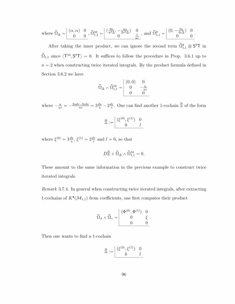
where rΩ∆ “pα, αq 0
0 0, rΩ10
1,1 “p 9αu2∆
,´ uα2v2∆
q 00 1
uv
, and rΩ91,1 “
p0,´ 5α4v∆q 0
0 0.
After taking the inner product, we can ignore the second term rΩ91,1 b S9T in
rΩ1,1 since xT10, S9Ty “ 0. It suffices to follow the procedure in Prop. 3.6.1 up to
n “ 2 when constructing twice iterated integrals. By the product formula defined in
Section 3.6.2 we have
rΩ∆ ^ rΩ101,1 “
p0, 0q 00 ´ α
uv
0 0
where ´ αuv“ ´2udv´3vdu
uv“ 3du
u´ 2dv
v. One can find another 1-cochain rΞ of the form
rΞ :“pξp0q, ξp1qq 0
0 l
where ξp0q “ 3duu
, ξp1q “ 2dvv
and l “ 0, so that
DrΞ` rΩ∆ ^ rΩ101,1 “ 0.
These amount to the same information in the previous example to construct twice
iterated integrals.
Remark 3.7.4. In general when constructing twice iterated integrals, after extracting
1-cochains of K‚pM1,1q from coefficients, one first computes their product
rΩβ ^ rΩγ “
pΦp0q,Φp1qq 00 ξ0 0
.
Then one wants to find a 1-cochain
rΞ :“pξp0q, ξp1qq 0
0 l
96

so that DrΞ ` rΩβ ^ rΩγ “ 0. In our case, Φp0q and Φp1q are always 0, since all of our
1-forms involve α,9 and the wedge product of two such 1-forms is 0. For terms in
ξ, one could put those of the form duu
into ξp0q and those of the form dvv
into ξp1q.
The rest of the terms in ξ would be exact and can be written as dl for some l. Then
rΞ “ pξp0q, ξp1q; lq would be sufficient to construct twice iterated integrals.
9 cf. In [4] Brown and Hain work with a complex Ω‚pX,Vnqω that each form in their complexinvolves ω, which is 3α
2∆ in our notation.
97
4
Conclusion
Our result in Chapter 2 completes the algebraic de Rham theory for unipotent fun-
damental groups of once punctured elliptic curves. The (universal) elliptic KZB
connection plays a vital role, since it captures the variation of algebraic de Rham
structures of these unipotent fundamental groups. It is a flat, algebraic and regular
connection, which we have checked explicitly by writing down the formulas. These
long formulas and other complications suggest that it would not be easy in general
to find an explicit algebraic de Rham theory for unipotent fundamental groups of
smooth varieties over Q, even in the cases like curves of higher genus.
Our work in Chapter 3 is far from finished. We have constructed iterated integrals
of algebraic modular forms that provide all multiple modular values. The ones that
involve modular forms of the second kind are completely new. The next step is to
compute and study the periods of these newly constructed iterated integrals. Our
first task is to investigate periods of twice iterated integrals of modular forms of the
second kind. Brown [3, §8, §22] has shown that periods of twice iterated integrals of
Eisenstein series involve periods of cusp forms and multiple zeta values. We expect
that periods of twice, and higher length, iterated integrals of modular forms of the
98

second kind should be intimately related to special values of L-functions, and that
they may provide geometric explanations for the depth filtration of multiple zeta
values.
It is also natural to generalize our results to relative completions of modular
groups of higher level. Just like in the case of level one, in order to develop an
algebraic de Rham theory for the relative completion of a modular group of higher
level, we need to first find an algebraic de Rham structure on the abelianization of
the Lie algebra of its unipotent radical. We should be able to do this using a similar
Mayer–Viertoris type patching argument [7], and we need to consider modular forms
of the second kind and possibly of the third kind [27]. Then we should be able
to apply Chen’s method of power series connections, and to construct algebraic de
Rham structures on the relative completions of modular groups.
A long term program is to construct iterated extensions of motives associated to
modular forms. We need to incorporate both Hodge theory [18] and the theory of p-
adic modular forms [7] into our study of relative completions of modular groups and
their periods. It is our hope that eventually this will lead to a modular construction
of mixed Tate motives over cyclotomic fields [3].
99

Bibliography
[1] R. Bott, L.W. Tu: Differential Forms in Algebraic Topology, Graduate Texts inMathematics, 82. Springer-Verlag, New York-Berlin, 1982. xiv+331 pp. ISBN:0-387-90613-4
[2] F. Brown: Mixed Tate motives over Z, Ann. of Math. 175 (2012), 949–976.
[3] F. Brown: Multiple modular values and the relative completion of the fundamen-tal group of M1,1, [arXiv : 1407.5167]
[4] F. Brown, R. Hain: Algebraic de Rham theory for weakly holomorphic modularforms of level one, [arXiv : 1708.00652], 2017.
[5] D. Calaque, B. Enriquez, P. Etingof: Universal KZB equations: the elliptic case,in Algebra, arithmetic, and geometry: in honor of Yu. I. Manin. Vol. I, 165–266,Progr. Math., 269, Birkhauser, Boston, 2009, [arXiv : math0702670]
[6] K.T. Chen: Extension of C8 function algebra by integrals and Malcev completionof π1, Advances in Math. 23 (1977), no. 2, 181–210.
[7] R. Coleman: Classical and overconvergent modular forms, J. Theor. NombresBordeaux 7 (1995), no. 1, 333–365.
[8] P. Deligne: Equations differentielles a points singuliers reguliers, Lecture Notesin Mathematics, Vol. 163. Springer-Verlag, 1970.
[9] P. Deligne: Le groupe fondamental de la droite projective moins trois points, inGalois groups over Q (Berkeley, CA, 1987), 79–297, Math. Sci. Res. Inst. Publ.,16, Springer, 1989.
[10] P. Deligne: Theorie de Hodge II, Inst. Hautes Etudes Sci. Publ. Math. No. 40(1971), 5–57.
100

[11] I. Dolgachev: Weighted projective varieties, Group actions and vector fields(Vancouver, B.C., 1981), 34–71, Lecture Notes in Math., 956, Springer, Berlin,1982.
[12] B. Enriquez, P. Etingof: A tannakian interpretation of the elliptic infinitesimalbraid Lie algebras, 2017, [arXiv : 1709.03430]
[13] R. Hain: Iterated integrals and algebraic cycles: examples and prospects, Con-temporary trends in algebraic geometry and algebraic topology (Tianjin, 2000),55–118, Nankai Tracts Math., 5, World Sci. Publ., River Edge, NJ, 2002.
[14] R. Hain: Lectures on Moduli Spaces of Elliptic Curves, in TransformationGroups and Moduli Spaces of Curves, Advanced Lectures in Mathematics, editedby Lizhen Ji, S.-T. Yau no. 16 (2010), 95–166, Higher Education Press, Beijing,[arXiv : 0812.1803].
[15] R. Hain: Notes on the universal elliptic KZB equation, 2013, [arXiv : 1309.0580].
[16] R. Hain: On a generalization of Hilbert’s 21st problem, Ann. Sci. Ecole Norm.Sup. (4) 19 (1986), no. 4, 609–627.
[17] R. Hain: The geometry of the mixed Hodge structure on the fundamental group,Algebraic Geometry, Bowdoin, 1985 (Brunswick, Maine, 1985), 247–282, Proc.Sympos. Pure Math., 46, Part 2, Amer. Math. Soc., Providence, RI, 1987.
[18] R. Hain: The Hodge-de Rham theory of modular groups, in Recent Advances inHodge Theory, 2015, Cambridge University Press. [arXiv : 1403.6443]
[19] R. Hain: The Hodge-de Rham theory of relative Malcev completion, Ann. Sci.Ecole Norm. Sup., t. 31 (1998), 47–92
[20] R. Hain, M. Matsumoto: Universal mixed elliptic motives, 2015[arXiv : 1512.03975].
[21] V. Knizhnik, A. Zamolodchikov: Current algebras and the Wess–Zumino modelin two dimensions, Nuclear Phys. B 247 (1984), 83–103.
[22] A. Levin, G. Racinet: Towards multiple elliptic polylogarithms, preprint, 2007,[arXiv : math0703237].
[23] M. Luo: Algebraic de Rham theory for relative compleltion of SL2pZq, in prepa-ration, 2017.
101

[24] M. Luo: The elliptic KZB connection and algebraic de Rham theory for unipotentfundamental groups of elliptic curves, 2017, [arXiv : 1710.07691].
[25] Y. Manin: Iterated integrals of modular forms and noncommutative modularsymbols, Algebraic geometry and number theory, 565–597, Progr. Math., 253,Birkhauser, 2006.
[26] Y. Manin: Iterated Shimura integrals, Mosc. Math. J. 5 (2005), 869–881, 973.
[27] A. Scholl, M. Kazalicki: Modular forms, de Rham cohomology and congruences,Trans. Amer. Math. Soc. 368 (2016), no. 10, 7097–7117.
[28] J. Steenbrink: Mixed Hodge structures on the vanishing cohomology, Realand complex singularities (Proc. Ninth Nordic Summer School/NAVF Sympos.Math., Oslo, 1976), pp. 525–563. Sijthoff and Noordhoff, Alphen aan den Rijn,1977.
[29] A. Weil: Elliptic Functions According to Eisenstein and Kronecker, Ergebnisseder Mathematik und ihrer Grenzgebiete, Band 88. Springer-Verlag, Berlin-NewYork, 1976.
[30] D. Zagier: Periods of modular forms and Jacobi theta functions, Invent. Math.104 (1991), 449–465.
[31] S. Zucker: Hodge theory with degenerating coefficients: L2 cohomology in thePoincare metric, Ann. of Math. (2) 109 (1979), no. 3, 415–476.
102

Biography
Ma Luo was born on July 30, 1990, in Shanghai, China. He entered the School of
Mathematical Sciences at Peking University in 2009. He was awarded an Innovation
Award and a Youth Festival Scholarship from Peking University in 2011. He earned
a B.S. in Mathematics and Applied Mathematics from Peking University in 2012. He
subsequently joined the graduate program in mathematics at Duke University. He
was awarded Graduate School Summer Research Fellowship in 2014 and in 2015. Un-
der the supervision of Richard Hain, he is expected to obtain a Ph.D. in Mathematics
from Duke University in 2018. He has written two papers [23, 24], corresponding to
the two parts in this thesis. He will continue as a Postdoctoral Research Assistant
to work with Francis Brown at the Mathematical Institute, University of Oxford in
2018.
103