ALGEBRAIC CONSTRUCTION OF MORTAR FINITE ELEMENTSPACES WITH APPLICATION TO PARALLEL AMGE

TZANIO V. KOLEV, JOSEPH E. PASCIAK, AND PANAYOT S. VASSILEVSKI

Abstract. In this paper, we propose a parallelization of an algebraic multigrid algo-rithm for finite element problems using a version of AMGe based on element agglom-eration (agAMGe). Specifically, we start with a partitioning of the original domaininto subdomains with a generally unstructured finite element mesh on each subdomain.The agglomeration based AMGe from [19] is then applied independently in each subdo-main. Note that even if one starts with a conforming fine grid, independent coarseninggenerally leads to non-matching grids on coarser levels. To set up global problems oneach level, we develop a general dual basis mortar approach. Because the agAMGealgorithm produces abstractelements and faces defined as lists ofnodes, the mortar mul-tiplier spaces need to be constructed in a purely algebraic way. We propose an algebraicextension of the local (element-based) construction used for the construction of thedual finite element mortar multiplier basis for three dimensional problems described in[20, 4]. Finally, a multigrid-preconditioned solver is applied to the resulting sequence of(non-nested) spaces. Numerical results illustrating the computational behavior of thenew algebraic multigrid algorithm are presented.

1. Introduction

In this paper, we consider the problem of developing algebraic multigrid algorithms ina parallel computing environment. Let the computational domain Ω ⊂ Rd, d ∈ 2, 3be the union of polyhedral subdomains, Ω = ∪p

i=1Ωi. We assume that we are givenan unstructured mesh on each subdomain Ωi. This means that the meshes need notresult from a geometric refinement strategy. Moreover, the meshes need not align acrosssubdomain boundaries as long as the mesh on each subdomain aligns with the boundaryof the interfaces between subdomains. By an interface we mean the boundary sharedbetween two subdomains having positive measure in Rd−1.

We consider finite element approximation of second order elliptic problem (positivedefinite and symmetric) in two or three dimensions using the above meshes and a dualbasis mortar approach. Of course, our method still applies to the case when the globalfinite element mesh conforms across the subdomain interfaces, in which case, the mortarmethod need not be used on the finest level.

The mortar finite element method was introduced by Bernardi, et al. in [8, 9]. Thetheory was later developed in [5, 6]. It is a nonconforming domain decomposition tech-nique which is attractive because it is suitable for parallel implementation and allows

Date: July 24, 1997–beginning; Today is: May 14, 2003.1991 Mathematics Subject Classification. 65F10, 65N20, 65N30.Key words and phrases. mortar spaces, algebraic construction, parallel coarsening, AMG.This work was performed under the auspices of the U. S. Department of Energy by the University of

California Lawrence Livermore National Laboratory under contract W-7405-Eng-48.1

2 TZANIO V. KOLEV, JOSEPH E. PASCIAK, AND PANAYOT S. VASSILEVSKI

for independent meshing of the different parts of a complicated domain. The essentialingredient of this method is the construction of a discrete space on each interface calledthe space of mortar multipliers. The finite element solution is sought in a space of func-tions having jumps across the interfaces orthogonal to the multiplier spaces. This “weakcontinuity” condition is enough to obtain a uniquely solvable problem with solution asaccurate as in the usual finite element method. For example, in [20], the following errorestimate was obtained:

p∑

i=1

‖u − uh‖21,Ωi

≤ C

p∑

i=1

h2i ‖u‖

22,Ωi

,

where u is the exact solution, uh is the approximate solution and hi denotes the maximumdiameter of the elements (tetrahedra in this case) in Ωi. The above estimate is valid undersome abstract conditions on the multiplier spaces. In particular, it is required that eachmultiplier space contains the constant functions and that the dimension of the space isequal to the number of interior degrees of freedom on one, fixed, side of the interface.

A natural idea for constructing a multiplier space with local basis functions is to startwith the dual basis for the traces of finite element functions (from one side of the interface)on each face on the interface. Then, for each interior node one can define a multiplierbasis function by taking linear combinations of the dual basis functions on each face.It is proven in [20] that such a “dual basis” approach leads to a stable and optimallyconvergent approximation.

The goal of this paper is to generalize the above construction in the algebraic case.This means that we use an algebraic procedure to coarsen (in parallel) each subdomainindependently and extend the dual basis technique to the coarser levels.

The standard algebraic multigrid algorithm was introduced to obtain a solver for prob-lems posed on large unstructured grids with efficiency comparable to that of multilevelmethods for the geometrically refined case [23, 24]. Recently, a large number of papershave been published on algebraic multigrid methods that use additional information suchas the element stiffness matrices to construct more robust algorithms. For example, thealgebraic multigrid for finite element problems (AMGe) and its spectral version (spectralAMGe) are described in [12, 19] and [13], respectively. We will only consider agAMGefor coarsening on the subdomains in our work [19]. This is because agAMGe preservescertain topological properties which are necessary for our generalized mortar technique.We note that our construction carries over to the case of element agglomeration spectralAMGe without any difficulty.

In the agAMGe discussion, we will closely follow the definitions and setting from[25]. For the most part, the exposition is algebraic even though, with agAMGe, thenotion of elements is preserved on the coarser “grids”. Specifically, one defines coarserelements as the union of finer elements mimicking the geometric refinement situation.Other topological properties such as element faces, domain boundaries, and nodes alsogeneralized to the coarser levels. This is important as the restrictions of elements to theinterface (the union of faces) is a critical ingredient in the algebraic mortar method whichwe propose here.

Roughly speaking, coarse elements in agAMGe are an agglomeration (union) of finegrid elements. Their degrees of freedom (nodes) are algebraically defined and associated

ALGEBRAIC CONSTRUCTION OF MORTAR FINITE ELEMENT SPACES 3

with a subset of the fine degrees of freedom through an interpolation matrix P . Thedetails of specific agAMGe constructions of P can be found in the references given above.

We will get global problems on the coarser “grids” by extending the dual basis multi-plier approach to the present algebraic setting. Using these global coarser grid problemsin combination with the multigrid strategy leads to a new parallelizable algebraic multi-grid algorithm. Because of the way that the spaces are glued together at the boundary,the coarser grid problems are not nested and so the resulting multigrid algorithm is notvariational. For the analysis of non-variational multigrid algorithms, see [10, 11].

In constructing the ingredients of the multigrid algorithm, i.e., the interpolation andsmoothing operators, we will mimic the geometric case in which the grids are obtained byuniform refinement. We will follow [17] where a variable V-cycle preconditioner resultingin a uniformly preconditioned algebraic system was presented.

There are other approaches for developing parallel algebraic multigrid algorithms. Forexample, in [14, 18] a specially designed coarsening procedure was used that resultedin a globally conforming mesh. The advantage of our approach is that we can use anyserial coarsening procedure, in particular, an element-based one such as agAMGe (whichproduces a better interpolation operator).

The remainder of the paper is outlined as follows. In §2, we set up the model problemand its discretization. The element agglomeration-based algebraic multilevel coarseningis summarized in §3. In §4, we extend the dual basis approach to the “generalized”finite elements generated by independent algebraic coarsening on the subdomains. Inparticular, we show that this construction results in dual basis functions that reproduceconstants locally. This is a fundamental ingredient in the analysis of standard mortarmethods and seems important to incorporate into the algebraic setting. The parallelagAMGe algorithm is described in §5. Finally, in §6 we present numerical results thatdemonstrate the performance of the proposed multigrid algorithm.

2. The model problem and finite element approximation

In this section, we briefly review the dual basis mortar approach. We assume that weare given a generally unstructured finite element mesh T0, e.g., a tetrahedral partitioningof Ωi. The mesh is assumed to cover each subdomain Ωi exactly but across the subdomaininterfaces the mesh may be non-matching. We only consider interfaces of positive measurein Rd−1 denoted by Γij ≡ ∂Ωi ∩ ∂Ωj. We assume that the mesh conforms with theinterfaces, i.e., the boundary of each interface Γij aligns with the meshes of both Ωi andΩj.

As a model problem, we consider the Dirichlet problem on a bounded polyhedraldomain Ω in Rd. Given f ∈ L2(Ω), we want to approximate the solution u ∈ H1

0 (Ω) of

(2.1)−∇ · (a∇u) = f in Ω,

u = 0 on ∂Ω.

Here a(x) is a positive function which is bounded above and bounded away from zero.Extensions to more general second order elliptic partial differential equations, systemsand to more general boundary conditions are possible and demonstrated in [1, 6]. Themortar method can be applied to a variety of other problems (see [2, 7, 21, 26]).

4 TZANIO V. KOLEV, JOSEPH E. PASCIAK, AND PANAYOT S. VASSILEVSKI

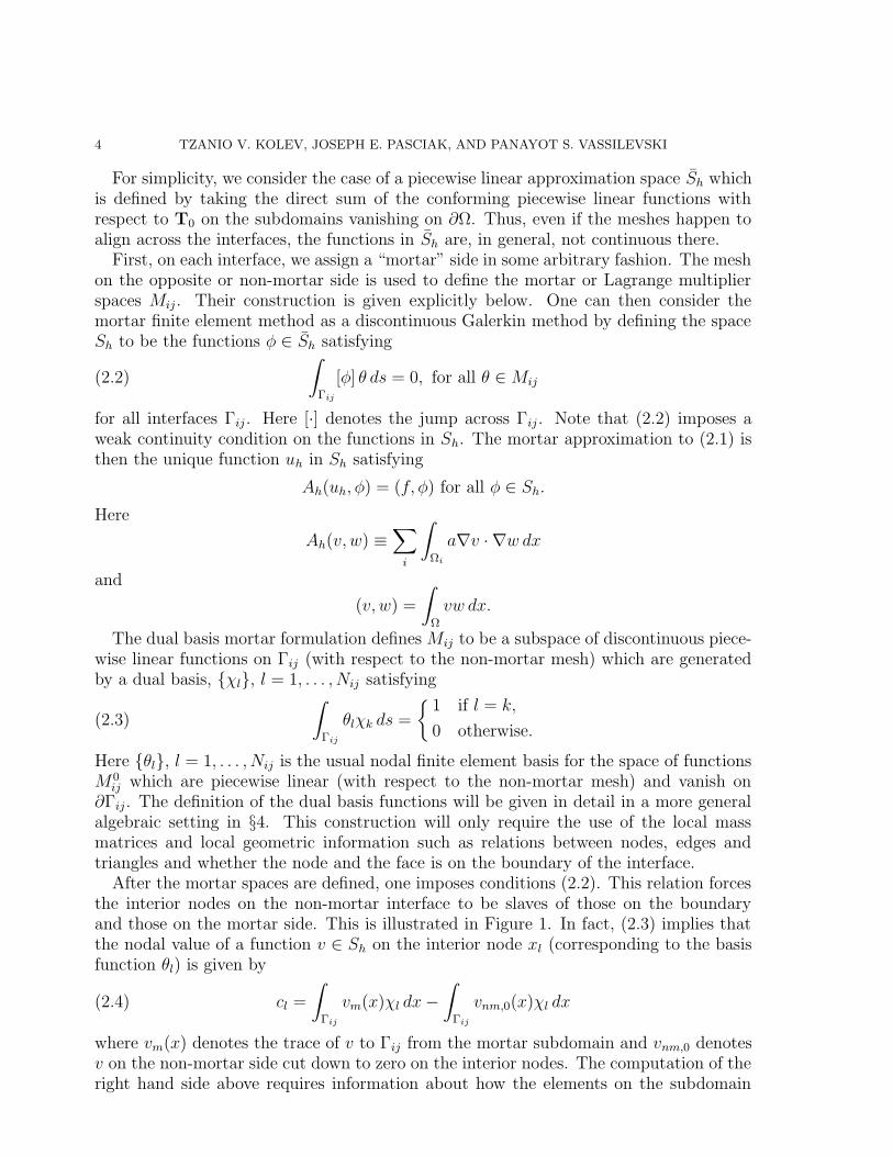
For simplicity, we consider the case of a piecewise linear approximation space Sh whichis defined by taking the direct sum of the conforming piecewise linear functions withrespect to T0 on the subdomains vanishing on ∂Ω. Thus, even if the meshes happen toalign across the interfaces, the functions in Sh are, in general, not continuous there.

First, on each interface, we assign a “mortar” side in some arbitrary fashion. The meshon the opposite or non-mortar side is used to define the mortar or Lagrange multiplierspaces Mij . Their construction is given explicitly below. One can then consider themortar finite element method as a discontinuous Galerkin method by defining the spaceSh to be the functions φ ∈ Sh satisfying

(2.2)

∫

Γij

[φ] θ ds = 0, for all θ ∈ Mij

for all interfaces Γij. Here [·] denotes the jump across Γij. Note that (2.2) imposes aweak continuity condition on the functions in Sh. The mortar approximation to (2.1) isthen the unique function uh in Sh satisfying

Ah(uh, φ) = (f, φ) for all φ ∈ Sh.

Here

Ah(v, w) ≡∑

i

∫

Ωi

a∇v · ∇w dx

and

(v, w) =

∫

Ω

vw dx.

The dual basis mortar formulation defines Mij to be a subspace of discontinuous piece-wise linear functions on Γij (with respect to the non-mortar mesh) which are generatedby a dual basis, χl, l = 1, . . . , Nij satisfying

(2.3)

∫

Γij

θlχk ds =

1 if l = k,

0 otherwise.

Here θl, l = 1, . . . , Nij is the usual nodal finite element basis for the space of functionsM0

ij which are piecewise linear (with respect to the non-mortar mesh) and vanish on∂Γij. The definition of the dual basis functions will be given in detail in a more generalalgebraic setting in §4. This construction will only require the use of the local massmatrices and local geometric information such as relations between nodes, edges andtriangles and whether the node and the face is on the boundary of the interface.

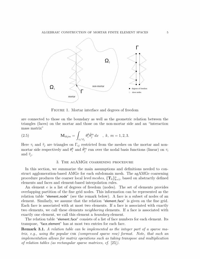
After the mortar spaces are defined, one imposes conditions (2.2). This relation forcesthe interior nodes on the non-mortar interface to be slaves of those on the boundaryand those on the mortar side. This is illustrated in Figure 1. In fact, (2.3) implies thatthe nodal value of a function v ∈ Sh on the interior node xl (corresponding to the basisfunction θl) is given by

(2.4) cl =

∫

Γij

vm(x)χl dx −

∫

Γij

vnm,0(x)χl dx

where vm(x) denotes the trace of v to Γij from the mortar subdomain and vnm,0 denotesv on the non-mortar side cut down to zero on the interior nodes. The computation of theright hand side above requires information about how the elements on the subdomain

ALGEBRAIC CONSTRUCTION OF MORTAR FINITE ELEMENT SPACES 5

Γ

Ω

Ω j

i

mortar

non-mortar

Γdegrees of freedom

slave nodes

Figure 1. Mortar interface and degrees of freedom

are connected to those on the boundary as well as the geometric relation between thetriangles (faces) on the mortar and those on the non-mortar side and an “interactionmass matrix”

(2.5) Mikjm =

∫

τi∩τj

θki θ

mj dx , k, m = 1, 2, 3.

Here τi and τj are triangles on Γij restricted from the meshes on the mortar and non-

mortar side respectively and θki and θm

j run over the nodal basis functions (linear) on τi

and τj.

3. The agAMGe coarsening procedure

In this section, we summarize the main assumptions and definitions needed to con-struct agglomeration-based AMGe for each subdomain mesh. The agAMGe coarseningprocedure produces the coarser local level meshes, Tk

nk=1, based on abstractly defined

elements and faces and element-based interpolation rules.An element e is a list of degrees of freedom (nodes). The set of elements provides

overlapping partition of the fine grid nodes. This information can be represented as therelation table “element node” (see the remark below). A face is a subset of nodes of anelement. Similarly, we assume that the relation “element face” is given on the fine grid.Each face is associated with at most two elements. If a face is associated with exactlytwo elements, we call these elements neighboring elements. If a face is associated withexactly one element, we call this element a boundary element.

The relation table “element face” consists of a list of face numbers for each element. Itstranspose, “face element” has at most two entries for each face.

Remark 3.1. A relation table can be implemented as the integer part of a sparse ma-trix, e.g., using the popular csr (compressed sparse row) format. Note, that such animplementation allows for matrix operations such as taking transpose and multiplicationof relation tables (as rectangular sparse matrices, cf. [25]).

6 TZANIO V. KOLEV, JOSEPH E. PASCIAK, AND PANAYOT S. VASSILEVSKI

Next, we consider the agglomeration AMGe algorithm, an algorithm that takes fineelements and faces and produces coarse elements and their faces. Each coarse elementE is defined as a list (or union) of fine elements. In practice, an agglomerated elementis a list of connected elements, i.e., the resulting union of fine grid elements represents asubset connected through their faces.

The coarse faces will be unions of fine faces. They are defined as follows:

(1) The coarse face associated with two coarse elements E1 and E2 is given by theunion of all fine faces shared by any pair of fine elements e1 ∈ E1 and e2 ∈ E2.

(2) The coarse face associated with a boundary element E is given by the union ofall fine faces corresponding to fine boundary elements e ∈ E.

The agAMGe coarsening algorithm produces the relation tables “coarse element fine

element”, “coarse element coarse face” and “coarse element coarse node,” extending the notionsof elements, faces and nodes to the coarser grids. From these one can, for example, buildthe relation table “coarse face coarse node”.

The relation between coarse basis functions and fine basis functions is defined througha sparse “prolongation” matrix P that interpolates values at the fine nodes from thoseat the coarse. This matrix has the structure “fine node coarse node”. Its transpose P t

defines the coarse grid nodal functions in terms of the fine. Specifically, the i’th coarsegrid nodal function is given by

θci =

∑

j

P tijθ

fj

where θfj denotes the set of fine grid basis functions. The above sum is taken over

integers j in the row of matrix “coarse node fine node” associated with the coarse nodeindex i. In our application, the coarsening procedure will be applied independently on thesubdomains and so the global matrix P will be a block diagonal matrix, one (rectangular)block for each subdomain.

We assume that P satisfies the following:

(1) When restricted to a coarse grid face, P has full column rank.(2) P has row-sum 1;

These requirements are met in the case of agAMGe applied to second order ellipticproblems of the form (2.1).

So that the interpolation procedure extends to the faces on the interfaces, some com-patibility constraints on the choice of the coarse nodes need to be imposed. Specifically,we shall assume:

Property 3.1. Fine nodes on a coarse face are interpolated only from coarse nodes onthat face.

The coarsening procedures in [19] satisfy these properties. The actual entries of theinterpolation matrix P are obtained by a certain energy minimization principle.

For a given subdomain, consider the finite element method based on its local fine-gridmesh T0 as discussed in the previous section. On each element e we have a set of nodalbasis functions corresponding to the degrees of freedom of e. We assume that we are giventhe local stiffness matrix Ae. The global matrix A (on each subdomain) is assembled in

ALGEBRAIC CONSTRUCTION OF MORTAR FINITE ELEMENT SPACES 7

the usual way,

wT Av =∑

e

wTe Aeve.

Here, ve = v|e denotes the restriction of v to the nodes of e.The coarse stiffness matrix Ac

E for each coarse element E is defined by assembling thelocal stiffness matrices Ae of its fine elements e ⊂ E:

(3.1) AcE =

∑

e∈E

(Re)T AeRe .

Here, Re has the rows of P corresponding to nodes of e.

4. Algebraic construction of mortar spaces

In this section, we present the algebraic element based construction of the mortarmultiplier spaces. This generalizes the dual basis approach from [20, 4] to the case ofmeshes which are generated using independent agAMGe coarsening on subdomains.

Note that on the finest level, an interface Γij is the union of faces from the mortar orthe non-mortar side. As noted in §3, this notion is preserved on the coarser grids. TheagAMGe algorithm respects these faces, i.e., Property 3.1 holds for them. Therefore,the agglomeration can be considered locally on each interface. As a consequence, thesubdomain interpolation matrices induce interface interpolation matrices. Thus, we candefine finite element spaces on both sides of the interface by taking the trace of thecorresponding subdomain finite element spaces. Moreover, the nested subdomain finiteelement spaces induce nested spaces on each side of each interface.

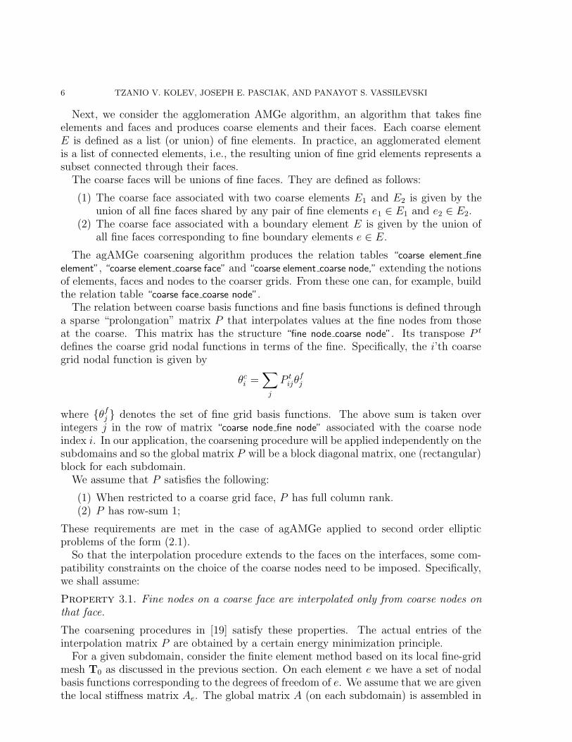
A node on Γij is called boundary if it also belongs to another interface. The nodeson Γij that are not boundary are called interior (to the interface). A face on Γij iscalled interior if it does not contain any boundary nodes, it is called a boundary face ifit contains interior and boundary nodes, and finally, it is called a corner face if it doesnot contain any interior nodes. This is illustrated in Figure 2.

corner

corner

interior boundary

Figure 2. Different types of faces on a non-mortar interface

8 TZANIO V. KOLEV, JOSEPH E. PASCIAK, AND PANAYOT S. VASSILEVSKI

For the purpose of constructing mortar spaces on the subdomain interfaces, one needsthe relations “mortar interface face” and “non-mortar interface face” on all levels. It is suffi-cient to construct the relation “coarse face fine face”. Then the required coarse relationsare obtained in terms of, e.g., the product

“mortar interface coarse face” = “mortar interface fine face” × “fine face coarse face”.Similarly, other relations between objects on both sides of a subdomain interface can becreated on all levels.

With the above structure, we can now define the generalized mortar method. Wewill consider a fixed interface Γij and the mesh structure corresponding to a fixed butarbitrary level of coarsening. We need to develop the analogies of Mij and M 0

ij (see §2).

The space M 0ij is defined to be the set of functions on the non-mortar mesh on Γij which

vanish on the boundary nodes of Γij. Let T be a non-mortar face of Γij and define Mij(T )to be the restriction of the non-mortar functions to T . This is a space of dimension equalto the number of nodes in the corresponding row of “non-mortar face non-mortar node”.The resulting mass matrix on the coarser levels can be assembled from that on the finer

using the “fine face coarse face” on the non-mortar subdomain. We define Mij = ⊕Mij(T )where the sum is taken over all faces of the non-mortar mesh on Γij. The space Mij will

be a subset of Mij .The dual basis functions in the finite element case (the finest grid in our application)

have two important properties:

(1) The dual basis functions are constructed locally.(2) The dual basis functions can reproduce constants locally.

These properties are fundamental in the analysis of the mortar method on the finer leveland we will reproduce them on the coarser levels.

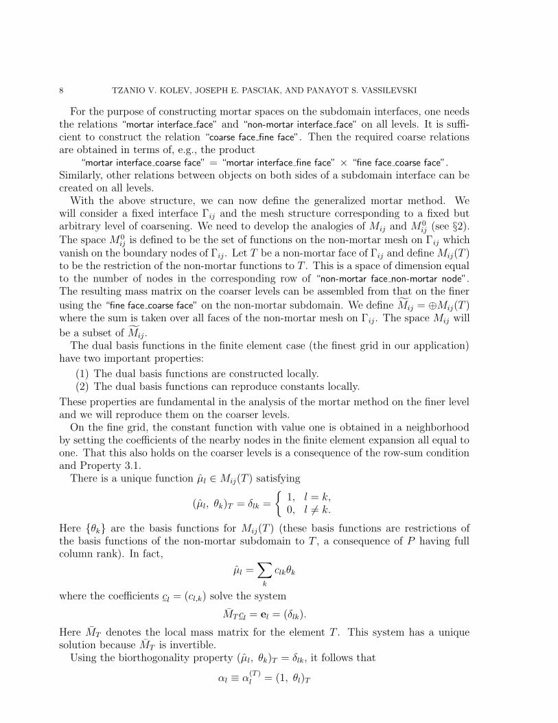
On the fine grid, the constant function with value one is obtained in a neighborhoodby setting the coefficients of the nearby nodes in the finite element expansion all equal toone. That this also holds on the coarser levels is a consequence of the row-sum conditionand Property 3.1.

There is a unique function µl ∈ Mij(T ) satisfying

(µl, θk)T = δlk =

1, l = k,

0, l 6= k.

Here θk are the basis functions for Mij(T ) (these basis functions are restrictions ofthe basis functions of the non-mortar subdomain to T , a consequence of P having fullcolumn rank). In fact,

µl =∑

k

clkθk

where the coefficients cl = (cl,k) solve the system

MT cl = el = (δlk).

Here MT denotes the local mass matrix for the element T . This system has a uniquesolution because MT is invertible.

Using the biorthogonality property (µl, θk)T = δlk, it follows that

αl ≡ α(T )l = (1, θl)T

ALGEBRAIC CONSTRUCTION OF MORTAR FINITE ELEMENT SPACES 9

satisfies ∑

l

αlµl = 1 on T.

The mortar multiplier basis functions µl are defined only for nodes xl that are interiorto Γij. We first assign corner faces T to nearby interior vertices, e.g., T is assigned to thenearest interior vertex. For each interior node xl and face T we define µl on T as follows:

(1) If T is a corner face assigned to xl then µl = 1 on T .(2) If T is a face which does not contain xl (excluding the case of (1) above) then

µl = 0 on T .(3) If T is a boundary face containing xl then

µl = αlµl + m−1∑

k: xk∈∂Γ∩T

αkµk on T

where m is the number of interior nodes in T .(4) If T is an interior face containing xl then µl = αlµl on T .

We then have1 =

∑µl on T

where the sum is taken over l such that µl 6= 0 on T .The space of mortar multipliers Mij is defined to be the span of µl. Note that the

dimension of Mij equals the number of interior nodes xl on Γ and it is easy to see that∫

Γij

µlθk ds = δlk

∫

Γij

µlθl ds.

The dual basis functions χl satisfying (2.3) are obtained from µl by the obviousscaling.

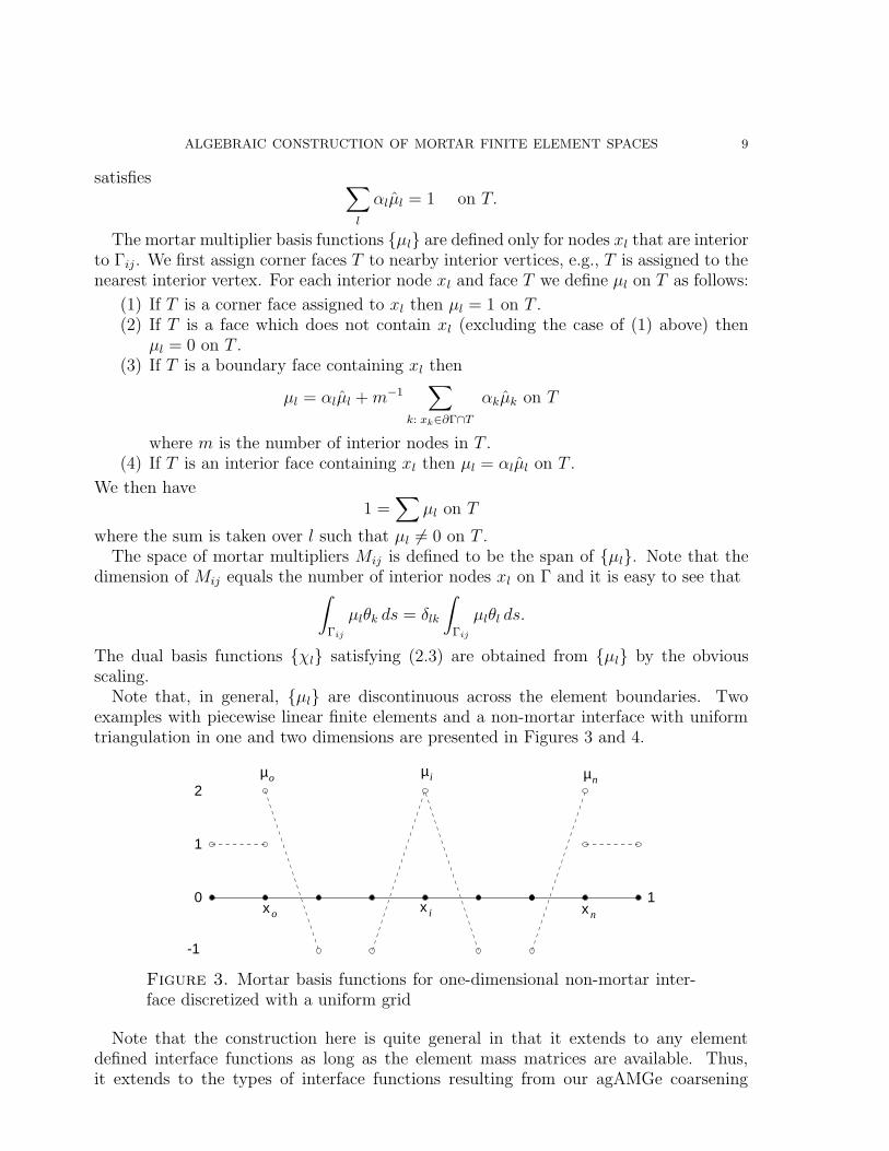
Note that, in general, µl are discontinuous across the element boundaries. Twoexamples with piecewise linear finite elements and a non-mortar interface with uniformtriangulation in one and two dimensions are presented in Figures 3 and 4.

o µi

ox x i

µn

x

µ

n

1

1

-1

2

0

Figure 3. Mortar basis functions for one-dimensional non-mortar inter-face discretized with a uniform grid

Note that the construction here is quite general in that it extends to any elementdefined interface functions as long as the element mass matrices are available. Thus,it extends to the types of interface functions resulting from our agAMGe coarsening

10 TZANIO V. KOLEV, JOSEPH E. PASCIAK, AND PANAYOT S. VASSILEVSKI

Figure 4. Mortar basis functions for two-dimensional non-mortar inter-face discretized with a uniform grid

procedure. It also extends to other finite element discretizations such as those usingnon-polynomial basis functions or non-conforming ones, such as the Crouzeix–Raviart,etc.

Since the dual basis for Mij and the basis for M 0ij are related by (2.3), the values of the

slave nodes on the interior of the non-mortar interface are given by (2.4) on any meshlevel. The implementation of this requires the corresponding interaction matrix (2.5).Note that since on both sides of the interface, the coarser elements on the face are madeup of finer elements, the coarser interaction matrix can be computed from the finer andthe relations “interface coarse face interface fine face” from the mortar and non-mortar sides.

5. Parallel AMGe

In this section, we describe the parallel multigrid algorithm based on local subdomainagAMGe coarsening. The implementation of this algorithm involves the following steps:

(1) Each subdomain is assigned to a processor which keeps its initial mesh and localelement matrices. Each interface is assigned to a processor.

(2) A fixed number of agAMGe-coarsening steps are performed in parallel on eachprocessor.

(3) The algebraic mortar spaces are constructed by the processors responsible for theinterfaces.

(4) The global matrix (reflecting the mortar constraints) is constructed using someparallel matrix storage structure on each grid level.

The above steps require significant communication between processors. For example,the processor responsible for an interface must gather coarsening data from both themortar and non-mortar subdomains (processors) at every coarsening step. Naturally, onewould assign an interface to one of the processors associated with one of the subdomainsso interprocessor communication would be required between only the two processorssharing the interface. Specifically, the processor on the interface constructs the localpart of the matrix P which implements the weak continuity condition (2.2). Locally, P

relates the non-mortar boundary nodes and the mortar interface nodes to the interiornon-mortar boundary nodes (slaves).

ALGEBRAIC CONSTRUCTION OF MORTAR FINITE ELEMENT SPACES 11

Mesh Generator

↓Problem Generator

↓hypre → Algebraic Solver ← AMGe

↓Visualization

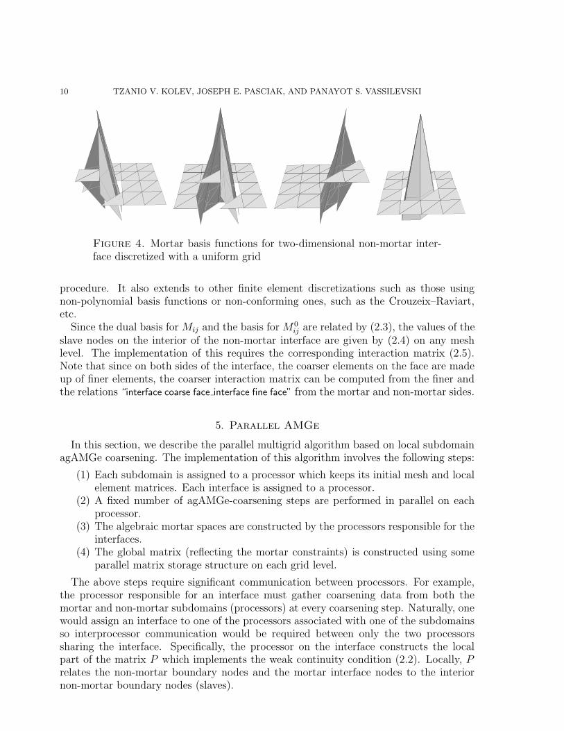
Figure 5. Software framework

For the multigrid interpolation, we follow [17]. Specifically, given a coarse grid function(satisfying the coarse grid constraints (2.2)), we interpolate locally on each subdomain.The resulting function does not satisfy the constraints on the finer grid. We impose theseconstraints on each interface by redefining the nodal values on the interior nodes on thenon-mortar side (slaves) using the formula (2.4). This redefinition requires communica-tion between the pair of processors representing the subdomains sharing the interface.

For the multigrid algorithm, we can use any standard smoother, e.g., those based onGauss-Seidel or Jacobi iteration. On the coarsest grid, we solve the problem exactly byconjugate gradient iteration to machine tolerance.

6. Numerical experiments

In this section, we discuss complexity issues, the behavior of the agAMGe coarseningand report the convergence behavior of the preconditioned algorithm using our mortar-based parallel AMGe algorithm.

The algorithm was implemented in a general, object-oriented MPI [22] code that usesparts of the HYPRE [15] preconditioning library. Specifically, the program constructs thestiffness matrix A and the mortar interpolation matrix P for each level and stores them inparallel (using the par csr format in HYPRE). The global matrix for the mortar methodis P tAP and is computed using a parallel triple matrix product (“RAP”) procedure fromHYPRE. The availability of the entries of this matrix allows the use of Gauss-Seidelsmoothing. Specifically, we use Gauss-Seidel with processors coloring [3]. This is aconvenient choice since, in contrast to Jacobi smoothing, its implementation does notrequire estimation of eigenvalues of the global matrix.

In our software framework, the geometric information provided by a mesh generatoris converted to algebraic information (i.e. relation tables, local mass matrices and localstiffness matrices) by a problem generator. This, in turn, is read by a solver which isindependent of the coordinates, the dimension, and the type of finite element basis func-tions used. Problem generators for model two-dimensional and general three-dimensionalproblems were implemented. These run in parallel refining independently in each subdo-main. They allow for general geometry including non-matching fine grids in three spatialdimensions. This software framework is illustrated in Figure 5.

A number of tests were performed to investigate the properties of the method. Thegeneral observation is that the method is reasonably scalable when the number of proces-sors is increased and the size of the problem in each processor is kept constant. The setup

12 TZANIO V. KOLEV, JOSEPH E. PASCIAK, AND PANAYOT S. VASSILEVSKI

cost, as with many other algebraic multigrid approaches, is high but remains bounded asthe number of processors increase. The solution time also scales well if we ignore the timefor the exact solve on the coarsest level of the multigrid. The latter starts to dominatewhen large number of processors are used. Efficiently dealing with the coarse solve is atopic for future research.

We consider the problem (2.1), where f ≡ 1, Ω is the unit square and a is describedbelow. In this test, we increase the number of processors while keeping the size of theproblem on each processor the same (64x64).

We used the preconditioned conjugate gradient algorithm with the mortar-based par-allel multigrid algorithm as a preconditioner. The stopping criterion was the reductionof the residual in the preconditioner norm by 6 orders of magnitude. All tests were runon ASCI Blue Pacific in LLNL.

Below we show the behavior of agAMGe coarsening in one interior subdomain.

• level 0: 4225 nodes, 8192 elements, 12416 faces• level 1: 1089 nodes, 2049 elements, 3107 faces• level 2: 306 nodes, 519 elements, 809 faces• level 3: 92 nodes, 135 elements, 221 faces• level 4: 32 nodes, 37 elements, 66 faces

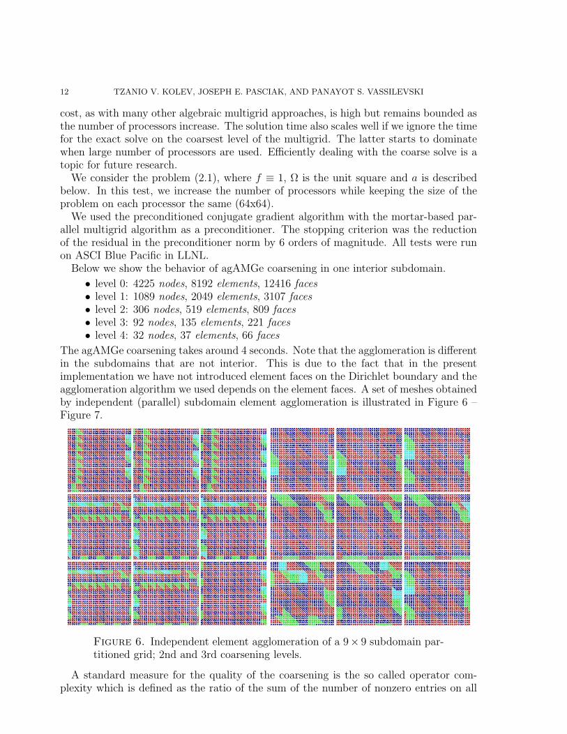
The agAMGe coarsening takes around 4 seconds. Note that the agglomeration is differentin the subdomains that are not interior. This is due to the fact that in the presentimplementation we have not introduced element faces on the Dirichlet boundary and theagglomeration algorithm we used depends on the element faces. A set of meshes obtainedby independent (parallel) subdomain element agglomeration is illustrated in Figure 6 –Figure 7.

Figure 6. Independent element agglomeration of a 9× 9 subdomain par-titioned grid; 2nd and 3rd coarsening levels.

A standard measure for the quality of the coarsening is the so called operator com-plexity which is defined as the ratio of the sum of the number of nonzero entries on all

ALGEBRAIC CONSTRUCTION OF MORTAR FINITE ELEMENT SPACES 13

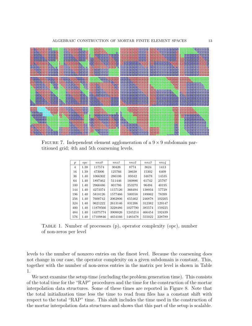
Figure 7. Independent element agglomeration of a 9× 9 subdomain par-titioned grid; 4th and 5th coarsening levels.

p opc nnz0 nnz1 nnz2 nnz3 nnz4

4 1.38 117574 30426 8774 3624 1413

16 1.39 473006 125766 38638 15302 6409

36 1.40 1066302 286106 89342 34678 14535

64 1.40 1897462 511446 160886 61742 25797

100 1.40 2966486 801786 253270 96494 40195

144 1.40 4273374 1157126 366494 138934 57729

196 1.40 5818126 1577466 500558 189062 78399

256 1.40 7600742 2062806 655462 246878 102205

324 1.40 9621222 2613146 831206 312382 129147

400 1.40 11879566 3228486 1027790 385574 159225

484 1.40 14375774 3908826 1245214 466454 192439

576 1.40 17109846 4654166 1483478 555022 228789

Table 1. Number of processors (p), operator complexity (opc), numberof non-zeros per level

levels to the number of nonzero entries on the finest level. Because the coarsening doesnot change in our case, the operator complexity on a given subdomain is constant. This,together with the number of non-zeros entries in the matrix per level is shown in Table1.

We next examine the setup time (excluding the problem generation time). This consistsof the total time for the “RAP” procedures and the time for the construction of the mortarinterpolation data structures. Some of these times are reported in Figure 8. Note thatthe total initialization time less the time to read from files has a constant shift withrespect to the total “RAP” time. This shift includes the time used in the construction ofthe mortar interpolation data structures and shows that this part of the setup is scalable.

14 TZANIO V. KOLEV, JOSEPH E. PASCIAK, AND PANAYOT S. VASSILEVSKI

416 36 64 100 144 196 256 324 400 484 576 676

10

20

30

40

50

60

70

80

90

100

110

120

130

140

Setup times

Number of processors

Tim

e (s

ec)

Total setupReading of input files in the memoryTotal setup − Reading inputRAP (all levels)

Figure 8. Setup times

Next, we look at the convergence behavior and solution times. We start with a smoothcoefficient problem (2.1) where a(x, y) = 1 + x2 + y2. In Table 2, we report the numberof unknowns, the asymptotic convergence factor, an estimate for the condition numberand the number of iterations corresponding to a v-cycle multigrid preconditioner withone pre and post smoothing. The estimate for the condition number was produced fromparameters in the conjugate gradient iteration based on a Lanczos procedure [16]. Allthese quantities clearly indicate convergence which is uniform in the number of processors.

p N ρ κ nit

4 16900 0.066 1.40 6

16 67600 0.071 1.42 6

36 152100 0.070 1.41 6

64 270400 0.070 1.41 6

100 422500 0.070 1.41 6

144 608400 0.070 1.41 6

196 828100 0.070 1.42 6

256 1081600 0.070 1.42 6

324 1368900 0.070 1.42 6

400 1690000 0.070 1.42 6

484 2044900 0.070 1.42 6

576 2433600 0.070 1.42 6

676 2856100 0.070 1.42 6

Table 2. Number of processors (p), total number of unknowns (N), as-ymptotic convergence factor (ρ), (estimate for) the condition number (κ),number of iterations (nit).

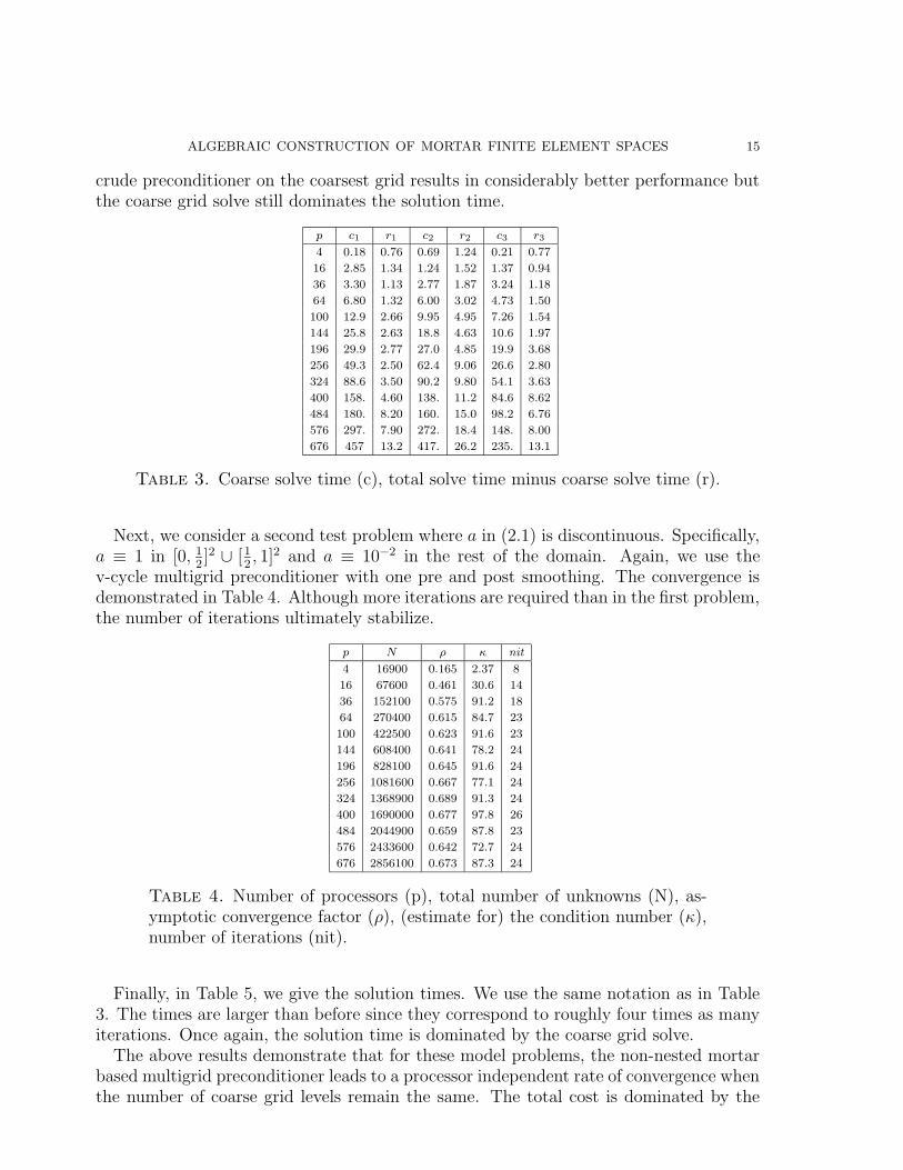
Next, in Table 3, we show the time for solution on the coarse grid (c) and the remainderof the time spent in solution procedure (r). This information is repeated for three differentchoices of the preconditioner, the standard V-cycle (1), the variable V-cycle (2) and astandard V-cycle where the coarse grid solve is preconditioned with the Gauss-Seidelsmoother (3). One can see that the coarse solve dominates the solution phase. This isa typical behavior of all domain decomposition based methods. Note that the use of a

ALGEBRAIC CONSTRUCTION OF MORTAR FINITE ELEMENT SPACES 15

crude preconditioner on the coarsest grid results in considerably better performance butthe coarse grid solve still dominates the solution time.

p c1 r1 c2 r2 c3 r3

4 0.18 0.76 0.69 1.24 0.21 0.77

16 2.85 1.34 1.24 1.52 1.37 0.94

36 3.30 1.13 2.77 1.87 3.24 1.18

64 6.80 1.32 6.00 3.02 4.73 1.50

100 12.9 2.66 9.95 4.95 7.26 1.54

144 25.8 2.63 18.8 4.63 10.6 1.97

196 29.9 2.77 27.0 4.85 19.9 3.68

256 49.3 2.50 62.4 9.06 26.6 2.80

324 88.6 3.50 90.2 9.80 54.1 3.63

400 158. 4.60 138. 11.2 84.6 8.62

484 180. 8.20 160. 15.0 98.2 6.76

576 297. 7.90 272. 18.4 148. 8.00

676 457 13.2 417. 26.2 235. 13.1

Table 3. Coarse solve time (c), total solve time minus coarse solve time (r).

Next, we consider a second test problem where a in (2.1) is discontinuous. Specifically,a ≡ 1 in [0, 1

2]2 ∪ [1

2, 1]2 and a ≡ 10−2 in the rest of the domain. Again, we use the

v-cycle multigrid preconditioner with one pre and post smoothing. The convergence isdemonstrated in Table 4. Although more iterations are required than in the first problem,the number of iterations ultimately stabilize.

p N ρ κ nit

4 16900 0.165 2.37 8

16 67600 0.461 30.6 14

36 152100 0.575 91.2 18

64 270400 0.615 84.7 23

100 422500 0.623 91.6 23

144 608400 0.641 78.2 24

196 828100 0.645 91.6 24

256 1081600 0.667 77.1 24

324 1368900 0.689 91.3 24

400 1690000 0.677 97.8 26

484 2044900 0.659 87.8 23

576 2433600 0.642 72.7 24

676 2856100 0.673 87.3 24

Table 4. Number of processors (p), total number of unknowns (N), as-ymptotic convergence factor (ρ), (estimate for) the condition number (κ),number of iterations (nit).

Finally, in Table 5, we give the solution times. We use the same notation as in Table3. The times are larger than before since they correspond to roughly four times as manyiterations. Once again, the solution time is dominated by the coarse grid solve.

The above results demonstrate that for these model problems, the non-nested mortarbased multigrid preconditioner leads to a processor independent rate of convergence whenthe number of coarse grid levels remain the same. The total cost is dominated by the

16 TZANIO V. KOLEV, JOSEPH E. PASCIAK, AND PANAYOT S. VASSILEVSKI

p c1 r1 c2 r2 c3 r3

4 0.60 0.98 0.56 1.21 0.35 1.02

16 15.2 2.40 10.8 3.03 4.05 2.09

36 50.0 4.03 42.6 6.59 12.6 3.18

64 110. 5.74 80.0 7.51 24.9 6.18

100 140. 6.27 121. 12.7 34.5 9.22

144 231. 8.26 180. 15.2 50.0 8.54

196 374. 12.9 278. 19.6 84.8 12.9

256 411. 14.9 393. 27.4 118. 11.3

324 579. 16.2 543. 41.0 215. 17.9

400 991. 28.9 828 46.5 365. 21.7

484 1084 25.7 1017 53.5 461. 28.5

576 1416 33.2 1394 85.6 827. 26.5

Table 5. Coarse solve time (c), total solve time minus coarse solve time (r).

coarse grid solve for a large number of processors. Setup costs are dominated by theinput phase while the costs for mortar interpolation and “RAP” are similar to the timespent in the solution phase excluding the coarse grid solve.

References

[1] Y. Achdou. The mortar element method for convection diffusion problems. C. R. Acad. Sci. ParisSer. I Math., 321(1):117–123, 1995.

[2] Y. Achdou, J.-C. Hontand, and O. Pironneau. A mortar element method for fluids. In Domain de-composition methods in sciences and engineering (Beijing, 1995), pages 351–360. Wiley, Chichester,1997.

[3] M. F. Adams. A distributed memory unstructured Gauss-Seidel algorithm for multigrid smoothers.In ACM/IEEE Proceedings of SC2001: High Performance Networking and Computing, Denver,Colorado, November 2001.

[4] W. Barbara. A mortar finite element method using dual spaces for the lagrange multiplier. SIAMJournal of Numerical Analysis, 38(3):989–1012, 2000.

[5] F. B. Belgacem. The mortar finite element method with lagrange multipliers. Numer. Math.,84:2173–2197, 1999.

[6] F. B. Belgacem and Y. Maday. The mortar finite element method for three dimensional finiteelements. Math. Model. Numer. Anal., 31:289–302, 1997.

[7] F. Ben Belgacem, A. Buffa, and Y. Maday. The mortar method for the Maxwell’s equations in 3D.C. R. Acad. Sci. Paris Ser. I Math., 329(10):903–908, 1999.

[8] C. Bernardi, Y. Maday, and A. T. Patera. Domain decomposition by the mortar element method.In H. G. Kaper and M. Garbey, editors, Asymptotic and Numerical Methods for Partial DifferentialEquations with Critical Parameters, pages 269–286. Kluwer Academic Publishers, Dordrecht, TheNetherlands, 1993.

[9] C. Bernardi, Y. Maday, and A. T. Patera. A new nonconforming approach to domain decomposition:The mortar element method. In H. Brezis and J.-L. Lions, editors, Nonlinear Partial DifferentialEquations and Their Applications, number 299 in Pitman Res. Notes Math., pages 13–51. LongmanScientific and Technical, Harlow, UK, 1994.

[10] J. H. Bramble, J. E. Pasciak, and J. Xu. The analysis of multigrid algorithm with nonnested spacesor noninherited quadratic forms. Math. Comp., 56:1–34, 1991.

[11] J. H. Bramble and X. Zhang. The Analysis of Multigrid Methods, volume 7 of Handbook of NumericalAnalysis. Elsevier, 2000.

ALGEBRAIC CONSTRUCTION OF MORTAR FINITE ELEMENT SPACES 17

[12] M. Brezina, A. J. Cleary, R. D. Falgout, V. E. Henson, J. E. Jones, T. A. Manteuffel, S. F.McCormick, and J. W. Ruge. Algebraic multigrid based on element interpolation (AMGe). SIAMJournal on Scientific Computing, 22:1570–1592, 2000.

[13] T. Chartier, R. Falgout, V. Henson, J. Jones, T. Manteuffel, S. McCormick, J. Ruge, , and P. S.Vassilevski. Spectral AMGe. SIAM Journal on Scientific Computing, 2003. (to appear).

[14] A. J. Cleary, R. D. Falgout, V. E. Henson, and J. E. Jones. Coarse-grid selection for parallel algebraicmultigrid. In Fifth International Symposium on Solving Irregularly Structured Problems in Parallel,volume 1457 of Lecture Notes in Computer Science, pages 104–115. Springer-Verlag, New York,1998.

[15] R. Falgout and U. Yang. hypre: a library of high performance preconditioners. In P. Sloot, C. Tan.,J. Dongarra, and A. Hoekstra, editors, Computational Science - ICCS 2002 Part III, volume 2331of Lecture Notes in Computer Science, pages 632–641. Springer-Verlag, 2002.

[16] G. H. Golub and C. F. V. Loan. Matrix Computations. 2nd ed. Johns Hopkins Press, Baltimore,MD., 1989.

[17] J. Gopalakrishnan and J. E. Pasciak. Multigrid for the mortar finite element method. SIAM Journalof Numerical Analysis, 37:1029–1052, 2000.

[18] V. E. Henson and U. M. Yang. BoomerAMG: a parallel algebraic multigrid solver and preconditioner.Applied Numerical Mathematics, 41:155–177, 2002.

[19] J. E. Jones and P. S. Vassilevski. AMGe based on element agglomeration. SIAM Journal on ScientificComputing, 23:109–133, 2001.

[20] C. Kim, R. D. Lazarov, J. E. Pasciak, and P. S. Vassilevski. Multiplier spaces for the mortar finiteelement method in three dimensions. SIAM Journal of Numerical Analysis, 39:519–538, 2001.

[21] L. Marcinkowski. A mortar element method for some discretizations of a plate problem. Numer.Math., 93(2):361–386, 2002.

[22] The message passing interface standard. URL http://www-unix.mcs.anl.gov/mpi/.[23] J. W. Ruge and K. Stuben. Efficent solutions of finite difference and finite element equations by

algebraic multigrid (AMG). In S. F. McCormick, editor, Multigrid methods, volume 3 of Frontiersin applied mathematics, pages 73–130. SIAM, Philadelphia, 1987.

[24] K. Stuben. Algebraic multigrid (AMG): experiences and comparisons. Appl. Math. Comput., 13:419–452, 1983.

[25] P. S. Vassilevski. Sparse matrix element topology with application to AMG(e) and preconditioning.Numerical Linear Algebra with Applications, 9, 2002.

[26] L. F. Wang, Q. Xia, and Y. Chen. The mortar finite element method for non-self-adjoint andindefinite problems. J. Fudan Univ. Nat. Sci., 40(6):604–610, 2001.

Department of Mathematics, Texas A&M University, College Station, TX 77843-3368,

USA.

E-mail address: tkolev@math.tamu.edu, pasciak@math.tamu.edu

Center for Applied Scientific Computing, UC Lawrence Livermore National Labora-

tory, P. O. Box 808, L-560, Livermore, CA 94551, USA.

E-mail address: panayot@llnl.gov