Improved Linear Algebra Methods for Redshift Computation ...

Algebra and Computation
Ramprasad Saptharishi∗
TIFR, Mumbai
January 16th, 2017 – May 15th, 2017
Contents
I Group theoretic algorithms 4
1 Introduction 41.1 Bringing in group theory . . . . . . . . . . . . . . . . . . . . . . . . . 5
2 Crash course on Group Theory 52.1 Homomorphisms, kernels, normal subgroups etc. . . . . . . . . . 62.2 Group Actions . . . . . . . . . . . . . . . . . . . . . . . . . . . . . . . . 62.3 Orbits and stabilizers . . . . . . . . . . . . . . . . . . . . . . . . . . . 7
3 Studying huge groups 93.1 Algorithmic tasks given a succinct group . . . . . . . . . . . . . . . 93.2 Computing orbits and the orbit graph . . . . . . . . . . . . . . . . . 103.3 Computing stabilizers . . . . . . . . . . . . . . . . . . . . . . . . . . . 113.4 Membership testing . . . . . . . . . . . . . . . . . . . . . . . . . . . . 153.5 Computing the size of a group . . . . . . . . . . . . . . . . . . . . . . 183.6 Normal closures and subnormality . . . . . . . . . . . . . . . . . . . 193.7 Commutators and solvability . . . . . . . . . . . . . . . . . . . . . . 20
4 Towers of subgroups 234.1 Set stabilizers, group intersection, and graph isomorphism . . . . 234.2 Descending towers . . . . . . . . . . . . . . . . . . . . . . . . . . . . . 244.3 Revisiting the group intersection problem . . . . . . . . . . . . . . 254.4 Solving an Automorphism Problem . . . . . . . . . . . . . . . . . . 27
5 Divide and Conquer techniques. 295.1 Intransitive case . . . . . . . . . . . . . . . . . . . . . . . . . . . . . . . 295.2 Blocks . . . . . . . . . . . . . . . . . . . . . . . . . . . . . . . . . . . . . 295.3 Block systems and structure forests . . . . . . . . . . . . . . . . . . . 315.4 Sylow Theorems and p-groups . . . . . . . . . . . . . . . . . . . . . 335.5 Divide and conquer via blocks . . . . . . . . . . . . . . . . . . . . . . 35
1
Contents
6 Colour Stabilizer for special groups 366.1 If G is not transitive . . . . . . . . . . . . . . . . . . . . . . . . . . . . 366.2 If G is not primitive . . . . . . . . . . . . . . . . . . . . . . . . . . . . . 36
7 Graph isomorphism for bounded degree graphs 387.1 Trivalent Graphs . . . . . . . . . . . . . . . . . . . . . . . . . . . . . . 397.2 Generalizing to higher (but bounded) degree graphs . . . . . . . . 43
8 General graph isomorphism 458.1 Colour Refinements . . . . . . . . . . . . . . . . . . . . . . . . . . . . 458.2 Reducing to the bounded generalized colour valence case . . . . . 478.3 GraphIso for bounded generalized colour valence graphs . . . . . 49
II Computations on polynomials 50
9 Preliminaries 519.1 Polynomial rings . . . . . . . . . . . . . . . . . . . . . . . . . . . . . . 529.2 Fraction fields . . . . . . . . . . . . . . . . . . . . . . . . . . . . . . . . 539.3 Finite fields . . . . . . . . . . . . . . . . . . . . . . . . . . . . . . . . . . 539.4 Adjoining elements and splitting fields . . . . . . . . . . . . . . . . 54
10 Basic operations on polynomials 5510.1 Polynomial multiplication . . . . . . . . . . . . . . . . . . . . . . . . 5610.2 Fast Fourier Transform . . . . . . . . . . . . . . . . . . . . . . . . . . . 5610.3 Polynomial division . . . . . . . . . . . . . . . . . . . . . . . . . . . . 6110.4 Multi-point evaluations . . . . . . . . . . . . . . . . . . . . . . . . . . 62
11 Factorizing univariate polynomials over finite fields 6311.1 Computing the GCD . . . . . . . . . . . . . . . . . . . . . . . . . . . . 6311.2 Handling repeated factors . . . . . . . . . . . . . . . . . . . . . . . . 6411.3 Some field properties, and Distinct Degree Factorization (DDF) . 6411.4 The Chinese Remainder Theorem . . . . . . . . . . . . . . . . . . . . 6611.5 The Cantor-Zassenhaus Algorithm . . . . . . . . . . . . . . . . . . . 6711.6 Berlekamp’s Algorithm . . . . . . . . . . . . . . . . . . . . . . . . . . 70
12 Factorizing Bivariate Polynomials over Finite Fields 7212.1 Hensel Lifting . . . . . . . . . . . . . . . . . . . . . . . . . . . . . . . . 7312.2 Bivariates as univariates over the fraction field . . . . . . . . . . . . 7412.3 The Resultant . . . . . . . . . . . . . . . . . . . . . . . . . . . . . . . . 75
13 Factorizing polynomials in Z[x] 8213.1 Finding a good prime . . . . . . . . . . . . . . . . . . . . . . . . . . . 8313.2 How large should k be? . . . . . . . . . . . . . . . . . . . . . . . . . . 8413.3 Lattices . . . . . . . . . . . . . . . . . . . . . . . . . . . . . . . . . . . . 8513.4 Gram-Schmidt Orthogonalization . . . . . . . . . . . . . . . . . . . . 86
14 Kaltofen’s black-box factorization algorithm 9314.1 Proof of Hilbert’s Irreducibility theorem . . . . . . . . . . . . . . . . 95
2

Contents
III Very Basic Algebraic Geometry 99
Last updated: Thu Apr 27 11:22:38 IST 2017
3
This course is going to be roughly split into three parts. The first part woulddeal with group theoretic algorithms and their application to the graph isomor-phism problem. The second part would deal with polynomials and factorizationalgorithms for them. The third part would deal with very basic algebraic geom-etry from a computational perspective.
Part I: Group theoretic algorithms
Lecture 1:January 16th, 2017 Notation
There may be moreto include... will addas they come end upbeing used
• We shall use Sn to denote the symmetric group on n elements. Sometimeswe might also look at a symmetric group action on a set A and we shalldenote that group by Sym(A)
• Groups will often be specified by a generating set. We shall denote this byG = ⟨S⟩.
• We shall use H ≤ G to denote that H is a subgroup of G.• We shall use H◁G to denote that H is a normal subgroup of G, and use
H ⊴ G to denote that H is a normal (not necessarily proper) subgroup ofG.
• Most of the groups considered in this course would be acting on a set Ω.We shall use the standard exponent notation, such as αg for α ∈ Ω andg ∈ G to denote the image of α under the action of g. This has the usefulproperty that (αg)h = αhg etc. The change in order is annoying but I preferthis as I want it to mimic h(g(α)).In the same notation, αG will denote the orbit of α under the action of G.
• If G acts on Ω and α ∈ Ω, we shall denote the stabilizer of α by stabG(α), orjust Gα.
1 Introduction
The first part of the course would focus on the Graph Isomorphism question.Definition 1.1 (Graph Isomorphism). Two graphs on n vertices G = (V, E) andH = (V, E′) are said to be isomorphic if there is a permutation σ ∈ Sn such that
(vi, vj) ∈ E⇐⇒ (vσ(i), vσ(j)) ∈ E′.
That is, there is a relabelling of the vertices such that edges and non-edges of G aremapped to edges and non-edges of H respectively.
◊
The computational task GraphIso is the task of checking if the two givengraphs G, H are isomorphic or not. What do we know about this problem?
Fact 1.2. GraphIso ∈ NP∩ co-AM.
4

2. Crash course on Group Theory
This intuitively suggests that GraphIso is unlikely to be NP-complete. In fact,recently there was a huge breakthrough by Babai1.
Theorem 1.3 (Babai). There is a deterministic algorithm for GraphIso running in timenpoly log n.
We would not be covering this result as a part of this course (alas!) but weshall however look at the technique of group theoretic algorithms developed byEugene Luks and Laszlo Babai to attack this problem.
1.1 Bringing in group theory
Let us ask a slightly different question. Suppose G and H were actually thesame graph. Now of course they are isomorphic because σ = id ∈ Sn preservesthe edge relations. But are there other non-trivial relabellings of vertices thatpreserve the edge relations? These are what are called automorphisms.Definition 1.4 (Graph Automorphisms). For a graph G = (V, E) on n vertices, theautomorphisms of G, denoted by Aut(G), is the following set of permutations:
Aut(G) = σ ∈ Sn ∶ (vi, vj) ∈ E⇐⇒ (vσ(i), vσ(j)) ∈ E . ◊
Observation 1.5. Aut(G) is a subgroup of Sn.
Understanding the group of automorphisms of a group turns out to be veryimportant for the question of graph isomorphism. Here is a concrete reason forit.
Lemma 1.6. Let G = (V, E) and H = (V′, E′) be two connected graphs on n vertices.Consider the graph X = (V ∪V′, E∪E′) which is just the union of the two graphs. Then,G is isomorphic to H if and only if there is a σ ∈ Aut(X) ⊆ S2n that maps some vertexof G (in X) to a vertex of H (in X).
Proof. Go figure.
Thus, if we could somehow get a handle on Aut(X), we may be able to checkif there are automorphisms that sort of swap G and H.
One issue here is that Aut(X) ⊆ S2n and hence can be a huge set (potentially allof S2n which has size (2n)!). Can we even hope to answer reasonable questionsfor such exponential sized groups? In this part of the course, we shall basicallybe addressing questions of this sort and eventually applying that to constructalgorithms for some special cases of GraphIso.
2 Crash course on Group TheoryThere is a seriesof fantastic blogposts by TimGowers on grouptheory. Highlyrecommended thatyou go over them atsome point.
I guess it is fair to assume that you know what a group is — a finite set with anassociative binary operation on it, with an identity, and inverses etc.
Here are some basic definitions/properties that one should know aboutgroups.
1This result is currently being peer-reviewed.
5

2. Crash course on Group Theory
Theorem 2.1 (Lagrange’s Theorem). If H is a subgroup of G (denoted by H ≤ G),then ∣H∣ divides ∣G∣.
One word proof: Cosets.
2.1 Homomorphisms, kernels, normal subgroups etc.
Definition 2.2 (Homomorphisms). A homomorphism is a map φ ∶ G → H betweentwo groups that behave well with the group multiplication in the sense that
• φ(idG) = idH ,• φ(g1g2) = φ(g1)φ(g2), and• φ(g−1) = (φ(g))−1. ◊
Once we have a homomorphism we can look at the kernel of the map φdefined by
ker(φ) = g ∈ G ∶ φ(g) = idH .
Proposition 2.3. Let φ ∶ G → H be a homomorphism between groups. Then, ker(φ) =
g ∈ G ∶ φ(g) = idH is a subgroup of G. Furthermore, it satisfies the property that
∀g ∈ G, k ∈ ker(φ) , gkg−1 ∈ ker(φ).
This idea of gkg−1 staying inside the subgroup is very useful property thatwe shall refer to such groups as normal subgroups.Definition 2.4 (Normal subgroups). A subgroup H is said to be a normal subgroupof G (denoted by H ⊴ G) if for every h ∈ H and g ∈ G we have that
ghg−1 ∈ H. ◊
Hence, Proposition 2.3 states that ker(φ) ⊴ G. Normal subgroups are ex-tremely useful and you can do operations on them that you typically cannot doon other subgroups.
Proposition 2.5. Let H ⊴ G and K ≤ G. Consider the set HK = hk ∶ h ∈ H , k ∈ K.Then, HK is a group.
One line proof: kh = h′k for some h′ ∈ H.
Proposition 2.6. Let H ⊴ G. Then, the set of cosets of H in G forms a group — thisis called the quotient group G/H. Furthermore, there is a natural homomorphismφ ∶ G → G/H for which ker(φ) = H.
There are many more properties that can be stated about normal subgroupsbut we’ll cross those bridges when we come to it.
2.2 Group Actions
But often, it is better to look at groups via its action on a set. Throughout thiscourse, we’ll only look at finite groups that act on a finite set.
6

2. Crash course on Group Theory
Definition 2.7 (Group actions). A group G is said to act on a set Ω if every g ∈ Ginduces a permutation of Ω (i.e. each g “moves” elements of Ω around) that satisfies thefollowing properties.
• id corresponds to the identity permutation. That is, αid = α for all α ∈ Ω,
• The actions compose in the natural way using the group multiplication — (αg)h = I prefer actions onthe left, hence thetwist in order.αhg. That is, moving α by g and then by h is the same as moving α by hg. ◊
A succinct way of saying this is that a group action is a homomorphism fromG to Sym(Ω) but the definition above spells out what this means. However, theaction could be redundant in the sense that there could be say two differentelements of G that induce the same permutation on Ω by their action. We shallsay that the action is faithful if the action of distinct elements of G is distinct. Orin other words, the homomorphism from G to Sym(Ω) is injective.
Observation 2.8. If G acts faithfully on a set Ω, then G is isomorphic to a subgroupof Sym(Ω).
Often in this course, G would actually be a subgroup of permutations onn elements so there is an immediate action of G on a set of n elements. Butsometimes the actions may not be immediate from the definition of the group.One specific example that is very relevant in this context is the action of a groupof n-permutations G ≤ Sn on Ω = ([n]
2 ) defined by
(i, j)σ = (σ(i), σ(j))
which is just lifting the action on vertices to edges.This part was notdone in the lecturebut might as wellkeep it here.
If G is a group of size n, then then there is a very natural standard action ofG on itself just defined by left-multiplication — gh = hg. It is easy to check thatthis is indeed a group action (called the left regular group action) by verifying allthe properties. Thus, one way to look at the elements of G is how it permutesthe elements of G upon left multiplication. This is formalized in the followingobservation.
Observation 2.9. Any group G with ∣G∣ = n is a subgroup of Sn, the symmetric groupon n elements.
A more interesting(?) action of G on itself is what is called the conjugationaction defined by gh = hgh−1. We’ll see more on these at a later point.
There is a lot that we can understand about a group from its action. We’llneed a few definitions.
2.3 Orbits and stabilizers
Definition 2.10 (Orbits). If G acts on Ω, the orbit of a point α ∈ Ω with respect tothe action of G (denoted by αG) is the set of all points that it can be moved to. Formally,
αG = β ∈ Ω ∶ β = αg for some g ∈ G . ◊
7
2. Crash course on Group Theory
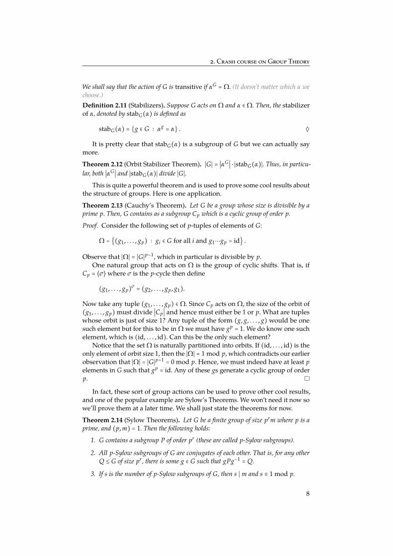
We shall say that the action of G is transitive if αG = Ω. (It doesn’t matter which α wechoose.)Definition 2.11 (Stabilizers). Suppose G acts on Ω and α ∈ Ω. Then, the stabilizerof α, denoted by stabG(α) is defined as
stabG(α) = g ∈ G ∶ αg = α . ◊
It is pretty clear that stabG(α) is a subgroup of G but we can actually saymore.
Theorem 2.12 (Orbit Stabilizer Theorem). ∣G∣ = ∣αG∣ ⋅ ∣stabG(α)∣. Thus, in particu-lar, both ∣αG∣ and ∣stabG(α)∣ divide ∣G∣.
This is quite a powerful theorem and is used to prove some cool results aboutthe structure of groups. Here is one application.
Theorem 2.13 (Cauchy’s Theorem). Let G be a group whose size is divisible by aprime p. Then, G contains as a subgroup Cp which is a cyclic group of order p.
Proof. Consider the following set of p-tuples of elements of G:
Ω = (g1, . . . , gp) ∶ gi ∈ G for all i and g1⋯gp = id .
Observe that ∣Ω∣ = ∣G∣p−1, which in particular is divisible by p.One natural group that acts on Ω is the group of cyclic shifts. That is, if
Cp = ⟨σ⟩ where σ is the p-cycle then define
(g1, . . . , gp)σ = (g2, . . . , gp, g1).
Now take any tuple (g1, . . . , gp) ∈ Ω. Since Cp acts on Ω, the size of the orbit of(g1, . . . , gp) must divide ∣Cp∣ and hence must either be 1 or p. What are tupleswhose orbit is just of size 1? Any tuple of the form (g, g, . . . , g) would be onesuch element but for this to be in Ω we must have gp = 1. We do know one suchelement, which is (id, . . . , id). Can this be the only such element?
Notice that the set Ω is naturally partitioned into orbits. If (id, . . . , id) is theonly element of orbit size 1, then the ∣Ω∣ = 1 mod p, which contradicts our earlierobservation that ∣Ω∣ = ∣G∣p−1 = 0 mod p. Hence, we must indeed have at least pelements in G such that gp = id. Any of these gs generate a cyclic group of orderp.
In fact, these sort of group actions can be used to prove other cool results,and one of the popular example are Sylow’s Theorems. We won’t need it now sowe’ll prove them at a later time. We shall just state the theorems for now.
Theorem 2.14 (Sylow Theorems). Let G be a finite group of size prm where p is aprime, and (p, m) = 1. Then the following holds:
1. G contains a subgroup P of order pr (these are called p-Sylow subgroups).
2. All p-Sylow subgroups of G are conjugates of each other. That is, for any otherQ ≤ G of size pr, there is some g ∈ G such that gPg−1 = Q.
3. If s is the number of p-Sylow subgroups of G, then s ∣ m and s ≡ 1 mod p.
8

3. Studying huge groups
3 Studying huge groups
Much of this part of the course would be dealing with groups acting on nelements, like symmetries of some graph on n vertices etc. A lot of times, thesecould be arbitrary subgroups of Sn which has n! elements in it. Therefore, wewould have to deal with subgroups G ≤ Sn that has exponentially many elementsin it. How is G to be provided to us?
Fortunately, we can succinctly specify large groups by providing a generatingset.Definition 3.1 (Generating set). A set S ⊆ G is said to be a generating set for Gis every element of G can be expressed as a product of elements in S (possibly usingelements of S multiple times). We shall denote this by G = ⟨S⟩. ◊
Lemma 3.2. Any finite group G has a generating set S of size O(log ∣G∣).
Proof. Let G be a finite group. If G is trivial, then ∅ ⊂ G generates G, and weare done. Suppose G is non-trivial, and pick a non-identity element x0 ∈ G. Thegroup G0 = ⟨x0⟩ generated by x0 satisfies G0 ≤ G and ⟨x0⟩ ≥ 2. If G0 = G, thenthe singleton set S0 ∶= x0 ⊂ G does the job. Else, there is x1 ∈ G ∖ G0 (andautomatically, x1 ∈ G is non-identity). Notice that the subgroup G1 = ⟨S1⟩ whereS1 ∶= S0 ∪ x0, satisfies G0 < G1 ≤ G (strictly contains G0 as a subgroup), andhence, by Lagrange’s theorem (Theorem 2.1), satisfies ∣G1∣ ≥ 2∣G0∣. We exploitthis observation to find a generating subset for G, of order O(log ∣G∣).
Set S−1 = G−1 ∶= ∅ ⊂ G. Having found a subset Sk−1 ⊂ G and the subgroupGk−1 ≤ G that it generates, we let Sk ∶= Sk−1 ∪ x for some x ∈ G ∖ Gk−1. Theprocess terminates because G is finite, and the resulting subset is indeed agenerating set because of the way it is constructed. On the other hand, if G = Gk,then
∣G∣ = ∣Gk∣ ≥ 2∣Gk−1∣ ≥ 22∣Gk−2∣ ≥ ⋯ ≥ 2k+1∣G−1∣ = 2k+1
which shows that ∣Sk∣ = k + 1 ≤ log ∣G∣. This proves the lemma since Sk ⊂ G is agenerating set.
With this, we can start asking a whole lot of questions given a succinctrepresentation of a group. First, we shall connect these questions to the graphisomorphism and graph automorphism questions.
3.1 Algorithmic tasks given a succinct groupLecture 2:January 20th, 2017 Membership: Given a group G ≤ Sn as G = ⟨S⟩ and a permutation σ ∈ Sn, check
if σ ∈ G.
Size of the group: Given a group G ≤ Sn as G = ⟨S⟩, compute ∣G∣.
Subgroup: Given two groups G, H ≤ Sn, presented as G = ⟨S⟩ and H = ⟨T⟩, checkif H ≤ G.
Normal subgroup: Given two groups G, H ≤ Sn, presented as G = ⟨S⟩ andH = ⟨T⟩, check if H ⊴ G.
9

3. Studying huge groups
Group Intersection: Given two groups G, H ≤ Sn, presented as G = ⟨S⟩ andH = ⟨T⟩, computing a generating set of G ∩ H.
Orbit computation: Given a group G ≤ Sn, presented as G = ⟨S⟩ acting onΩ = [n], compute the orbits of the group action.
Stabilizer computation: Given a group G ≤ Sn, presented as G = ⟨S⟩, acting onΩ = [n] and a point α ∈ Ω, compute a generating set of stabG(α).
Normalizer computation: Given a group G ≤ Sn, presented as G = ⟨S⟩, find theset of elements of Sn that normalizes G. That is,
NormalizerSn(G) = h ∈ Sn ∶ h−1gh ∈ G ∀g ∈ G .
Computing automorphisms of a graph: Given a graph G, compute a generatingset for Aut(G).
... and many more.
For each of the above problems, we shall either show that there are poly-nomial time algorithms or prove some sort of hardness result. Througout thissection, unless otherwise stated, when we say “Given input G = ⟨S⟩”, we shallmean that the input is the set S. Furthermore, we will always mean that G ≤ Snnaturally acts on Ω = 1, . . . , n.
3.2 Computing orbits and the orbit graph
We are given an input G = ⟨S⟩ and an α ∈ Ω and we want to compute its orbit
αG = β ∶ β = αg for some g ∈ G .
The following natural algorithm works.Algorithm 1: Orbit
Input : ⟨S⟩ and α ∈ ΩOutput :The orbit of α
1 ∆ = α2 while ∆ grows do3 for β ∈ ∆ and g ∈ S do4 if βg ∉ ∆ then5 ∆ = ∆ ∪ βg
6 return ∆
Correctness of the algorithm is evident. The algorithm runs while ∆ grows,and hence, there can be at most 1+ ∣αG ∣ ≤ 1+ n iterations of step 2, the additionalone being to verify that ∆ has stopped growing. In each iteration of step 2,the algorithm executes step 2 ≤ (∣αG ∣ ⋅ ∣S∣) ≤ n ⋅ ∣S∣ times, and for each of theseexecutions, carries out membership-check βG ∉ ∆ which takes ≤ ∣αG ∣ ≤ n times.Therefore, the running time of the algorithm is O((n + 1) ⋅ n ⋅ ∣S∣ ⋅ n) = O(n3∣S∣).
10

3. Studying huge groups
We can augment this algorithm to not just find the orbit, but find a represen-tative gα,β ∈ G such that αgα,β = β for every α, β from the same orbit.
Algorithm 2: OrbitRepresentativesInput : G = ⟨S⟩ and an α ∈ ΩOutput :A set of orbit representatives of α
1 X = (Ω,∅), the empty graph with vertices Ω2 for α ∈ Ω and g ∈ S do3 if (α, αg) is not a directed edge in X then4 Add the directed edge (α, αg) to X with label g.
5 Compute T, the connected component containing α.6 Let R = id
7 for every β ∈ T do8 Let gα,β be the (left-)product of edge labels of a path from α to β in X
so that gα,β maps α to β.9 Add gα,β to R.
10 return R
The strongly connected components of the orbit-graph X, constructed inthe above algorithm, are orbits induced by G. Furthermore, if α, β are in thesame orbit the above algorithm finds an element g ∈ G such that αg = β bytaking a path from α to β and multiply the edge labels along the way. We makea convention here, that our choice element g ∈ G satisfying αg = α will always bethe identity element of G.
Again this algorithm runs in poly(n, ∣S∣) time. Indeed, step 2 involves atmost (∣αG ∣ ⋅ ∣S∣) ≤ n∣S∣ execution of step 3, and for each execution of step 3, thealgorithm carries out at most ∣αG ∣2 ≤ n2 edge-membership checks. Therefore,computing the orbit graph takes O(n3∣S∣) time. Once we have the orbit graph,computing connected components, shortest paths etc. are clearly polynomialtime.
3.3 Computing stabilizers
Suppose that we are given as input a group G = ⟨S⟩ and a point α ∈ Ω. We wishto compute Gα = stabG(α) = g ∈ G ∶ αg = α.
Note that by Lagrange’s theorem, stabG(α) tiles G exactly. Also, by Theo-rem 2.12, the number of tiles is exactly the orbit size ∣αG∣. From this, what can wesay about the cosets of stabG(α)? These are sets of the form g ⋅Gα. If αg = β, thenevery element of g ⋅Gα moves α to β. Hence, the cosets of Gα exactly correspondsto fixing a β ∈ αG and collecting the set of all g ∈ G that maps α to β.
This (mis)leads us to consider the following “natural algorithm” for comput-ing a generating set for Gα.
11

3. Studying huge groups
Algorithm 3: Not-StabiliserGenSetInput : G = ⟨S⟩ and α ∈ ΩOutput :A generating set for Gα = stabG(α)
1 Using Algorithm 2, compute αG and a set of distinct representativesgβ ∶ β ∈ αG such that αgβ = β for every β ∈ αG.
2 Let T = ∅
3 for each g ∈ S do4 if αg = α then5 Add g to T6 else7 Let β = αg.8 Add g−1
β ⋅ g to T.
9 return T
Notice that the “generating set” T ⊂ G returned by our “natural algorithm”satisfies ∣S∣ = ∣T∣. Let us try proving correctness of this “algorithm”. For this, wemake the following observation: that the subset S′ ∶= T ∪gβ ∶ β ∈ αG generatesG, as this generates everything in the original generating set S. Now, in order toprove “correctness”, we just need to show the following
Not-a-Lemma. The set T that Algorithm 3 outputs is indeed a generating set forGα = stabG(α).
And here is how a possible proof might be sketched out.
(Incorrect) “Proof.” Firstly note that all the elements we add to T in line 8 areindeed in T. So certainly H = ⟨T⟩ ≤ Gα. To show that H = Gα, observe thatT ∪ gβ ∶ β ∈ αG generate G as they clearly generate everything in S. But then, This sentence isn’t
true...this can at most give ∣αG∣ distinct cosets of ⟨T⟩. The only way this can cover allof G is if ∣H∣ ⋅ ∣αG∣ = ∣G∣ which forces H = stabG(α). ?QED?
Unfortunately, as the title indicates, Not-a-lemma is indeed not a lemma. Wefirst consider an example that will show that T ⊂ stabα(G) is not a generatingset of stabα(G). We didn’t do this
counter-example inclass but thanks toSomnath for this!
Example 3.3. Consider the symmetric group S10 of permutations of the set 0, 1,⋯, 9,and let the cyclic permutations σ0, σ3, σ6 ∈ S10, be given as follows: σ0 = (0 1 2), σ3 =
(3 4 5), σ6 = (6 7 8). The subset T′ ∶= σ0, σ3, σ6 ⊂ S10 generates a subgroup of S10.Let us write H′ = ⟨T′⟩. Since σiσj = σjσi for all i, j ∈ 0, 3, 6, the subgroup H′ ≤ S10 iscommutative, and the non-identity elements of H′ can have order 3 only; in particular,H′ is not cyclic since there is no element of order 27 = ∣H′∣. Now consider any 2-elementssubset T2 ∶= h1, h2 ⊂ H′. The subgroup ⟨T2⟩ ≤ H′ has order ≤ 9. Therefore, H′ cannot have a generating set of less than three elements. Notice that the elements in H′ areall even permutations, and therefore, H′ ≤ A10, where A10 ≤ S10 is the alternating group.
Recall that S10 has a generating set of size 2. Thus, if it was known that H′ ≤ S10is the stablizer of some element under some group-action, then we could have directlycontradicted the statement of Not-a-lemma. And this is easy to come-up with. Let
12

3. Studying huge groups
m ∶= [S10 ∶ H′] be the number of cosets of H′ ≤ S10, and let Ω = id, x1,⋯, xm−1 ⊂ S10be a complete set of coset-representatives. Explicitly, m = (10)!/27. Define action of S10on Ω as follows: for g ∈ G and x ∈ Ω, set xg = xi if and only if gx ∈ xi H. Finally, notethat H = stabS10(id).
Note that the action we have just defined does not really “look like” the natural actionof Sn on 1,⋯, n. However, that is only superficial. As the definition of group actionsuggested, this action induces a homomorphism S10 → Sm whose kernel is the subgroupK ∶= ∩g∈S10 gH′g−1. Notice that K ≤ S10 is a normal subgroup of S10, contained inH′ ≤ A10, and has order ≤ 27; therefore, K ⊴ A10 is a proper normal subgroup. SinceA10 is simple, this shows that K ≤ H′ is trivial. Thus, the action we defined is justinduced by the natural action of Sm on the set 1,⋯, m, up to relabelling of the elementsof Ω. ◊
What went wrong with the proof then? Well, an element g ∈ G, as we haveobserved, can be written as g = g1⋯gt with all gi ∈ S′ = T ∪ gβ ∶ β ∈ αG. Letus suppose that g ∉ ⟨T⟩; then there is some gk ∈ gβ ∶ β ∈ αG appearing in theabove expression such that gk+1,⋯, gt ∈ T. For our line of argument in the above“proof” to work, we need a gβ, β ∈ αG such that g1⋯gk ∈ gβ H, or equivalently,g−1
β (g1⋯gk−1)gk ∈ H. However, we are now in hopeless situation, since the “al-gorithm” did not assure us of even having gk−1gk ∈ gβH for some β ∈ αG.
Lecture 3:January 23rd, 2017 Heaven is not lost! Although our algorithm could not return what it was
expected to, we have a clue as to what could be a way around. Notice thatwe have derived the following in our preceding discussion: in order for T′ ⊂stabG(α) to be a generating set, we needed to have g−1
β (g1⋯gk−1)gk ∈ H for someβ ∈ αG, whenever gk ∈ gβ ∶ β ∈ αG and gi ∈ T ∪ gβ ∶ β ∈ αG. We formulateour revamped strategy along this lines.
This restrictionof id ∈ R canbe removed. SeeLemma 3.6 fora more generalstatement.
Lemma 3.4. Let G = ⟨S⟩ be acting on Ω = 1,⋯, n and R = x1,⋯, xm ⊂ G acomplete set of orbit-representatives and assume id ∈ R. For any g ∈ G and xi ∈ R, thereexists a unique xj ∈ R such that x−1
j gxi ∈ stabG(1).
Proof. In fact, this lemma is almost a tautology. For any g ∈ G and xi ∈ R, if 1xi g = jthen there is a unique x ∈ R such that 1xj = j; this is because R = x1,⋯, xm ⊂ Ga complete set of orbit-representatives. But this implies x−1
j gxi ∈ stabG(1).
Let us consider T ∶= x−1j gxi ∶ g ∈ S, xi, xj ∈ R, x−1
j gxi ∈ stabG(1). We havethe following
Lemma 3.5. Every g ∈ G can be written as g = xit for a unique xi ∈ R and uniquet ∈ ⟨T⟩.
Proof. If g = id, there is nothing to prove. Else, write g = gkgk−1⋯g1 with gi ∈ Sfor all 1 ≤ i ≤ k. Recall that our convention was to have id ∈ R. Assume that k = 1in the expression g = gkgk−1⋯g1, so that g ∈ S. Since id ∈ R, the above lemmatells us that there is a unique x ∈ R such that x−1g ∈ stabG(1). By definition of T,we have x−1g ∈ T; since g = x(x−1g), we are done.
13

3. Studying huge groups
We now proceed via induction on k. Assume the induction hypothesis; thatis, for every string gkgk−1⋯g1 ∈ G, where gi ∈ S for all 1 ≤ i ≤ k, there is a xk ∈ Rand t ∈ ⟨T⟩ such that
gkgk−1⋯g1 = xk t
Ô⇒ g = gk+1gkgk−1⋯g1 = gk+1 xk t.
By the Lemma 3.4, there is a unique xk+1 ∈ R such that x−1k+1gk+1xk ∈ stabG(1), and
by definition of T, again t′k ∶= x−1k+1gk+1xk ∈ T. But this implies g = xk+1(x−1
k+1gk+1xk)tk =
xk+1t′kt
g = gk+1 xkt
= xk+1 (x−1k+1 gk+1 xk) t
= xk+1 t′kt
∈ xk+1 ⟨T⟩ .
This proves the lemma modulo the uniqueness part.
Now to the uniqueness. Notice that T ⊂ stabG(1), and hence, ⟨T⟩ ≤ stabG(1).Supose that xiti = xjtj for some ti, tj ∈ ⟨T⟩ and xi, xj ∈ R; then we have x−1
i xj =
tit−1j ∈ ⟨T⟩ ⊂ stabG(1), which shows that 1xi = 1xj . This implies xi = xj since R
contains a unique representative for each l ∈ 1G. But then ti = tj.
We now have an algorithm to find the generating set of stabG(α), for α ∈ Ω.
Algorithm 4: StabiliserGenSetInput : G = ⟨S⟩ and α ∈ ΩOutput :A generating set for Gα = stabG(α)
1 Using Algorithm 2, compute the orbit αG ⊂ Ω and a complete set ofdistinct coset-representatives R ∶= gβ ∶ β ∈ αG, such that αgβ = β forevery β ∈ αG, and gα = id.
2 Let T = ∅
3 for each g ∈ S and gβ, gγ ∈ R, do4 if g−1
β g gγ fixes α then5 Add g−1
β g gγ to T
6 return T
Invoking Algorithm 2 costs O(n3∣S∣) time. Step 3 involves ≤ n2∣S∣ runs, andeach run involves checking if the orbit graph contains the edge (γ, β) whichinvolves at most ≤ n2 time. Therefore, the running time of this algorithm ispolynomial in n and ∣S∣. To show the correctness of the algorithm, notice thatT ⊂ stabG(α), and hence, ⟨T⟩ ≤ stabG(α). Now suppose g ∈ G is any element; byLemma 3.5, there is a unique gβ ∈ R such that g ∈ gβt for some t ∈ ⟨T⟩. That is,there can be at most ∣αG∣ distinct cosets of ⟨T⟩
14
3. Studying huge groups
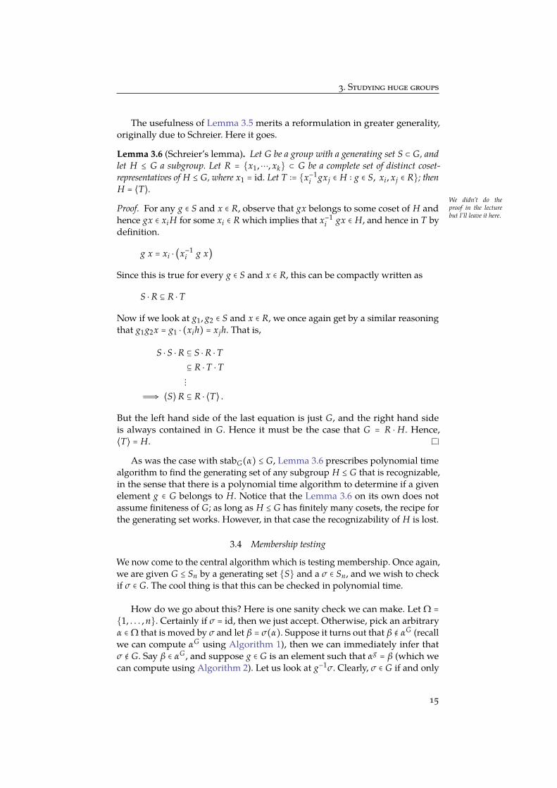
The usefulness of Lemma 3.5 merits a reformulation in greater generality,originally due to Schreier. Here it goes.
Lemma 3.6 (Schreier’s lemma). Let G be a group with a generating set S ⊂ G, andlet H ≤ G a subgroup. Let R = x1,⋯, xk ⊂ G be a complete set of distinct coset-representatives of H ≤ G, where x1 = id. Let T ∶= x−1
i gxj ∈ H ∶ g ∈ S, xi, xj ∈ R; thenH = ⟨T⟩.
We didn’t do theproof in the lecturebut I’ll leave it here.
Proof. For any g ∈ S and x ∈ R, observe that gx belongs to some coset of H andhence gx ∈ xi H for some xi ∈ R which implies that x−1
i gx ∈ H, and hence in T bydefinition.
g x = xi ⋅ (x−1i g x)
Since this is true for every g ∈ S and x ∈ R, this can be compactly written as
S ⋅ R ⊆ R ⋅ T
Now if we look at g1, g2 ∈ S and x ∈ R, we once again get by a similar reasoningthat g1g2x = g1 ⋅ (xih) = xjh. That is,
S ⋅ S ⋅ R ⊆ S ⋅ R ⋅ T
⊆ R ⋅ T ⋅ T
⋮
Ô⇒ ⟨S⟩ R ⊆ R ⋅ ⟨T⟩ .
But the left hand side of the last equation is just G, and the right hand sideis always contained in G. Hence it must be the case that G = R ⋅ H. Hence,⟨T⟩ = H.
As was the case with stabG(α) ≤ G, Lemma 3.6 prescribes polynomial timealgorithm to find the generating set of any subgroup H ≤ G that is recognizable,in the sense that there is a polynomial time algorithm to determine if a givenelement g ∈ G belongs to H. Notice that the Lemma 3.6 on its own does notassume finiteness of G; as long as H ≤ G has finitely many cosets, the recipe forthe generating set works. However, in that case the recognizability of H is lost.
3.4 Membership testing
We now come to the central algorithm which is testing membership. Once again,we are given G ≤ Sn by a generating set S and a σ ∈ Sn, and we wish to checkif σ ∈ G. The cool thing is that this can be checked in polynomial time.
How do we go about this? Here is one sanity check we can make. Let Ω =
1, . . . , n. Certainly if σ = id, then we just accept. Otherwise, pick an arbitraryα ∈ Ω that is moved by σ and let β = σ(α). Suppose it turns out that β ∉ αG (recallwe can compute αG using Algorithm 1), then we can immediately infer thatσ ∉ G. Say β ∈ αG, and suppose g ∈ G is an element such that αg = β (which wecan compute using Algorithm 2). Let us look at g−1σ. Clearly, σ ∈ G if and only
15

3. Studying huge groups
if g−1σ ∈ G. What have we gained? The key point is that g−1σ does not move α,i.e g−1σ (α) = α. Hence, we have the following simple observation.
Observation 3.7. If σ(α) = β and if αg = β for some g ∈ G; then, σ ∈ G if and only ifg−1σ ∈ stabG(α).
By Algorithm 4, we can construct a generating set for stabG(α) in polynomialtime. We just recursively keep applying the above observation. This results inthe following algorithm for membership testing.
Algorithm 5: MembershipTest(E)Input : G = ⟨S⟩ and σ ∈ SnOutput :Yes if σ ∈ G, and No otherwise.
1 if σ = id then2 return Yes
3 Since σ ≠ id, let α ∈ Ω such that σ(α) = β ≠ α.4 if β ∉ αG then5 return No
6 Since β ∈ αG, using Algorithm 2 compute an element g ∈ G such thatαg = β.
7 Using Algorithm 4, compute a generating set T for stabG(α).8 return MembershipTest(E)(T, g−1σ)
The correctness of the algorithm is clear. However, there is a catch. The size ofthe successive generating sets grows as ∣TstabG(α)∣ ≤ ∣S∣ ⋅ ∣αG ∣, without an apparentreasonable bound. On the other hand, it is apparent that having some bound ofthe form ∣T∣ ∈ O(nk), for example, will turn Algorithm 5 into a polynomial timealgorithm. This is accomplished as follows.
Suppose that a group G ≤ Sn is given as G = ⟨S⟩. We intend to find T ⊂ Gsuch that ∣T∣ ≤ n2, and G = ⟨T⟩. The following algorithm builds a strictly upper-triangular n × n tableau M in which, each cell holds at most one element of G,and the cells on/below the diagonal are empty.
16

3. Studying huge groups
Algorithm 6: ReduceGenSetInput : G = ⟨S⟩, where S is given as an array S = g1,⋯, gk
Output :A generating set for G of size at most n2
1 Let M[i][j] = ∅ for all integers i, j = 1,⋯, n2 Let t = 13 while t ≤ k, do4 if gt = id then5 t ←Ð t + 1
6 else7 Let i be the smallest index such that igt ≠ i and Let j ∶= ig.8 if M[i][j] = ∅ then9 insert g in M[i][j]
10 t ←Ð t + 1
11 else12 Replace gt in S by g′ ∶= (M[i][j])−1g.
13 return M
Notice that this is a polynomial time algorithm because each execution of thewhile loop may involve at most n repetitions each of which is polynomial-step.Moreover, in each stage, the set M ∪ gt+1,⋯, gk forms a generating set for G.Therefore, the algorithms ends with a generating set, namely, the set of elementsin the tableau M; the size of this set is ≤ (n
2) ≤ n2.
Following modification of the preceding membership testing algorithm (Al-gorithm 5) now yields a polynomial time algorithm.
Algorithm 7: MembershipTest(S, σ)
Input : G = ⟨S⟩ and σ ∈ SnOutput :Yes if σ ∈ G, and No otherwise.
1 if σ = id then2 return Yes
3 Since σ ≠ id, let α ∈ Ω such that σ(α) = β ≠ α.4 if β ∉ αG then5 return No
6 Since β ∈ αG, using Algorithm 2 compute an element g ∈ G such thatαg = β.
7 Using Algorithm 4, compute a generating set T for stabG(α).8 return MembershipTest(ReduceGenSet(T), g−1σ)
Now that we have membership testing, a lot of other natural problems followalmost immediately. For example, given two groups H and G, we can test if
17

3. Studying huge groups
H ≤ G.
Algorithm 8: SubgroupTestInput : G = ⟨S⟩ and H = ⟨T⟩
Output :Yes if H ≤ G, and No otherwise.1 for each h ∈ T do2 if MembershipTest(S, h) = No then3 return No
4 return Yes
We can also check if H ⊴ G.
Algorithm 9: NormalSubgroupTestInput : G = ⟨S⟩ and H = ⟨T⟩
Output :Yes if H ⊴ G, and No otherwise.1 if SubgroupTest(S, T) = No then2 return No3 for each g ∈ S and h ∈ T do4 if MembershipTest(T, ghg−1) = No then5 return No
6 return Yes
3.5 Computing the size of a group
Given a group G = ⟨S⟩, we wish to compute ∣G∣. The following natural attemptthat uses the Orbit-Stabilizer theorem ( Theorem 2.12) works.
Algorithm 10: GroupSizeInput : G = ⟨S⟩Output : ∣G∣
1 if S = ∅ then2 return 1
3 Let α ∈ Ω with ∣αG∣ > 14 Compute r = ∣αG∣ using Algorithm 1.5 Compute a generating set T of size at most n2 for stabG(α) using
Algorithm 4 and Algorithm 6.6 Recursively compute M = GroupSize(T) = ∣stabG(α)∣.7 return r ⋅ M
But if we were to unravel the recursion, we get a chain of subgroups of Gthat are successive stabilizers. Let Ω = 1, . . . , n. For any group G ≤ Sn, we shalldefine the following groups:
G(i) = g ∈ G ∶ jg = j for all j ≤ i .
18
3. Studying huge groups
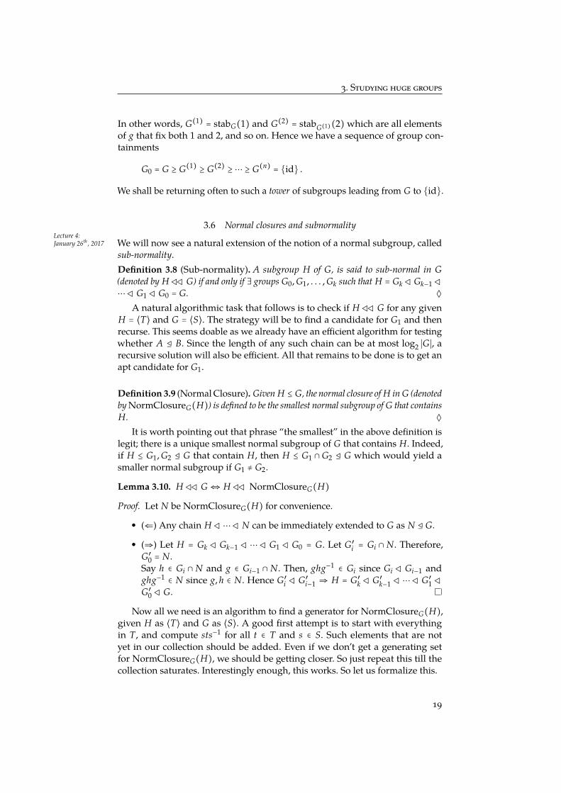
In other words, G(1) = stabG(1) and G(2) = stabG(1)(2) which are all elementsof g that fix both 1 and 2, and so on. Hence we have a sequence of group con-tainments
G0 = G ≥ G(1) ≥ G(2) ≥ ⋯ ≥ G(n) = id .
We shall be returning often to such a tower of subgroups leading from G to id.
3.6 Normal closures and subnormalityLecture 4:January 26th, 2017 We will now see a natural extension of the notion of a normal subgroup, called
sub-normality.Definition 3.8 (Sub-normality). A subgroup H of G, is said to sub-normal in G(denoted by H◁◁ G) if and only if ∃ groups G0, G1, . . . , Gk such that H = Gk ◁Gk−1 ◁
⋯◁G1 ◁G0 = G. ◊
A natural algorithmic task that follows is to check if H◁◁ G for any givenH = ⟨T⟩ and G = ⟨S⟩. The strategy will be to find a candidate for G1 and thenrecurse. This seems doable as we already have an efficient algorithm for testingwhether A ⊴ B. Since the length of any such chain can be at most log2 ∣G∣, arecursive solution will also be efficient. All that remains to be done is to get anapt candidate for G1.
Definition 3.9 (Normal Closure). Given H ≤ G, the normal closure of H in G (denotedby NormClosureG(H)) is defined to be the smallest normal subgroup of G that containsH. ◊
It is worth pointing out that phrase “the smallest” in the above definition islegit; there is a unique smallest normal subgroup of G that contains H. Indeed,if H ≤ G1, G2 ⊴ G that contain H, then H ≤ G1 ∩ G2 ⊴ G which would yield asmaller normal subgroup if G1 ≠ G2.
Lemma 3.10. H◁◁ G⇔ H◁◁ NormClosureG(H)
Proof. Let N be NormClosureG(H) for convenience.
• (⇐) Any chain H◁⋯◁ N can be immediately extended to G as N ⊴ G.
• (⇒) Let H = Gk ◁ Gk−1 ◁⋯◁ G1 ◁ G0 = G. Let G′i = Gi ∩ N. Therefore,
G′0 = N.
Say h ∈ Gi ∩ N and g ∈ Gi−1 ∩ N. Then, ghg−1 ∈ Gi since Gi ◁ Gi−1 andghg−1 ∈ N since g, h ∈ N. Hence G′
i ◁G′i−1 ⇒ H = G′
k ◁G′k−1 ◁⋯◁G′
1 ◁
G′0 ◁G.
Now all we need is an algorithm to find a generator for NormClosureG(H),given H as ⟨T⟩ and G as ⟨S⟩. A good first attempt is to start with everythingin T, and compute sts−1 for all t ∈ T and s ∈ S. Such elements that are notyet in our collection should be added. Even if we don’t get a generating setfor NormClosureG(H), we should be getting closer. So just repeat this till thecollection saturates. Interestingly enough, this works. So let us formalize this.
19

3. Studying huge groups
Algorithm 11: NormalClosureInput : G = ⟨S⟩ , H = ⟨T⟩
Output : B ∶ ⟨B⟩ = NormClosureG(H)
1 set B = T2 repeat3 set B ← B′
4 for each b ∈ B, s ∈ S do5 if MembershipTest(B′, ghg−1) = No then6 B′ ← B′ ∪ gbg−1
7 until B′ = B8 return B
Correctness: Every element that is added to B′ in the algorithm are clearlyelements that ought to be in NormClosureG(H). Furthermore, whenever thealgorithm terminates, the group generated by B′ is normal in G. Hence thealgorithm indeed outputs a generating set for the smallest normal subgroup ofG that contains H.
Running time: Every increase in size of B′ makes the group generated by B′
double in size. Hence, we have at most log2 (n!) iterations, each of which takespolynomial time.
Putting together all these ideas, we get the following algorithm for subnor-mality testing.
Algorithm 12: SubnormalityTestInput : G = ⟨S⟩ , H = ⟨T⟩
Output :Yes if H◁◁ G, No otherwise1 i ← 02 S0 ← S3 repeat4 i ← i + 15 Si ←NormalClosure(Si−1, T)
6 until ⟨Si⟩ = ⟨Si+1⟩
7 if ⟨Si⟩ = ⟨T⟩ then // Can be checked via Algorithm 7
8 return Yes9 else
10 return No
Remark. The above algorithm has the added bonus that if H◁◁ G, then the sets Si
computed in fact give generating sets for the subnormal chain between H and G. ◊
3.7 Commutators and solvability
A group G is said to be abelian if∀a, b ∈ G, we have ab = ba. As a natural extension,we want to comment about how close G is to being abelian. This notion goes via
20

3. Studying huge groups
something called a commutator subgroup of G.
Definition 3.11 (Commutator Subgroup). Let G be a group. The commutator sub-group of G, denoted by [G, G], is given by:[G, G] ∶= ⟨xyx−1y−1 ∶ x, y ∈ G⟩ ◊
Here is an important fact that we won’t prove in class.
Fact 3.12. [G, G] ⊴ G and G[G,G]
is abelian. Furthermore, [G, G] is the smallest normalsubgroup H ⊴ G such that G
H is abelian. That is, if H ⊴ G and GH is abelian, then
[G, G] ≤ H.
Task: Given G = ⟨S⟩, find a generating set for [G, G].
A guess would be again to try B ∶= ghg−1h−1 ∶ g, h ∈ S. This however maynot always work, since we are not guaranteed that the element, say, gghg−1g−1h−1
will be in ⟨B⟩. But, we know that H ∶= ⟨B⟩ ≤ [G, G] ⊴ G. Therefore our nexttry should be the normal closure of this H. Let us now verify that this willactually work. For that, it is enough to show that G
H′ is abelian, where H′ ∶=
NormClosureG(H). This follows from Fact 3.12.
Lemma. Given a group G = ⟨S⟩ and H ∶= xyx−1y−1 ∶ x, y ∈ S. If H′ ∶= NormClosureG(H),then G
H′ is abelian.
Proof. The intuition is that we know H′ contains xyx−1y−1 ∶ x, y ∈ S which inessence means that in the quotient group G
H′ , we have the “relations” xy = yx forall x, y ∈ S. Given the fact that every element of G is generated by S should allowus to permutate elements of G
H′ as well. The following proof formalizes this.
Claim. For every a, b ∈ G, there is some h ∈ H′ such that ab = ba ⋅ h.
Clearly, proving the above claim immediately implies that GH′ is abelian.
Pf. Firstly, if a, b ∈ S then we already∗ have a−1b−1ab ∈ H′ hence ∗ Wait, why? Weonly know thataba−1b−1
∈ H′...ah, because H′ isnormal.
ab = ba ⋅ a−1b−1ab. If a, b are “strings” in S, we shall prove the aboveclaim by induction on its length. Say a = a1⋯as and b = b1⋯bt, andsay t > 1 (the other case is symmetric). By the inductive hypothesis
a1⋯asb1⋯bt = b1⋯bt−1a1⋯as ⋅ h ⋅ bt (h ∈ H′)
= b1⋯bt−1a1⋯asbt(b−1t hbt)
= b1⋯bt−1a1⋯asbt ⋅ h′ (h′ ∈ H′ , normality)= b1⋯bt−1bta1⋯as ⋅ h′′ ⋅ h (induction)
which is what we set out to prove.
That finishes the proof of the claim and hence the lemma.
21
3. Studying huge groups
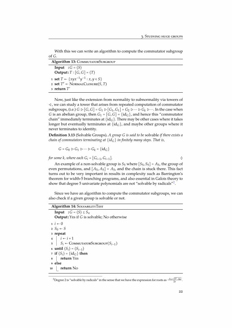
With this we can write an algorithm to compute the commutator subgroupof G.
Algorithm 13: CommutatorSubgroupInput : G = ⟨S⟩Output : T ∶ [G, G] = ⟨T⟩
1 set T ← xyx−1y−1 ∶ x, y ∈ S2 set T′ ← NormalClosure(S, T)3 return T’
Now, just like the extension from normality to subnormality via towers of◁, we can study a tower that arises from repeated computation of commutatorsubgroups, (i.e.) G▷ [G, G] = G1▷ [G1, G1] = G2▷⋯▷Gk ▷⋯. In the case whenG is an abelian group, then G1 = [G, G] = idG, and hence this “commutatorchain” immediately terminates at idG. There may be other cases where it takeslonger but eventually terminates at idG, and maybe other groups where itnever terminates to identity.Definition 3.13 (Solvable Groups). A group G is said to be solvable if there exists achain of commutators terminating at idG in finitely many steps. That is,
G = G0 ▷G1 ▷⋯▷Gk = idG
for some k, where each Gi = [Gi−1, Gi−1]. ◊
An example of a non-solvable group is S5 where [S5, S5] = A5, the group ofeven permutations, and [A5, A5] = A5, and the chain is stuck there. This factturns out to be very important in results in complexity such as Barrington’stheorem for width-5 branching programs, and also essential in Galois theory toshow that degree 5 univariate polynomials are not “solvable by radicals”2.
Since we have an algorithm to compute the commutator subgroups, we canalso check if a given group is solvable or not.
Algorithm 14: SolvabilityTestInput : G = ⟨S⟩ ≤ SnOutput :Yes if G is solvable; No otherwise
1 i ← 02 S0 ← S3 repeat4 i ← i + 15 Si ← CommutatorSubgroup(Si−1)
6 until ⟨Si⟩ = ⟨Si−1⟩
7 if ⟨Si⟩ = idG then8 return Yes9 else
10 return No
2Degree 2 is “solvable by radicals” in the sense that we have the expression for roots as −b±√
b2−4ac2a .
22
4. Towers of subgroups
4 Towers of subgroupsLecture 5:January 30th, 2017 So far, we have been looking at algorithmic tasks given a generating set for the
subgroup. But in often cases, we do not really have the generating set of thegroup we are interested in. Keep in mind the automorphisms of a graph; wedo not really have a generating set for this group but what we instead knowis to check if a given element is an automorphism or not. Often, existence of anice tower of subgroups from a known group to our target group can be veryuseful. To understand this better, let us look at a few computational problemsthat would be sufficient to solve graph isomorphism.
4.1 Set stabilizers, group intersection, and graph isomorphism
We have already seen the notion of stabilizer of a point α ∈ Ω. The following is ageneralization that applies to a subset ∆ ⊆ Ω.Definition 4.1 (Set Stabilizer). Given G = ⟨S⟩ ≤ Sn and ∆ ⊆ 1, 2, . . . , n, the stabi-lizer of ∆ in G denoted by SetStabG(∆) = g ∈ G ∶ ∆g = ∆, ∆g = ∆ ◊
Observation 4.2. SetStabG(∆) ≤ G.
We now want to show that GraphAut (a problem to which GraphIso can bereduced, as mentioned in Lemma 1.6), where we want to find the generatingset of Aut(X) given a graph X = (V, E) is reducible to SetStab, where we wantto find the generating set of SetStabG(∆) given G = ⟨S⟩ ≤ Sn and ∆ ⊆ 1, 2, . . . n.We formalize this as:
Lemma 4.3. GraphAut ≤TM SetStab. The ≤TM is a termi-nology used to saythat one problem isTuring Machine re-ducible to another.Or in simpler words,A ≤TM B is sayingthat the problem Bis at least as hard asproblem A computa-tionally.
Proof. Suppose X = (V, E) is a graph with ∣V∣ = n. Given an oracle which com-putes SetStabG(∆) for every G and ∆, we want to compute GraphAut(X).
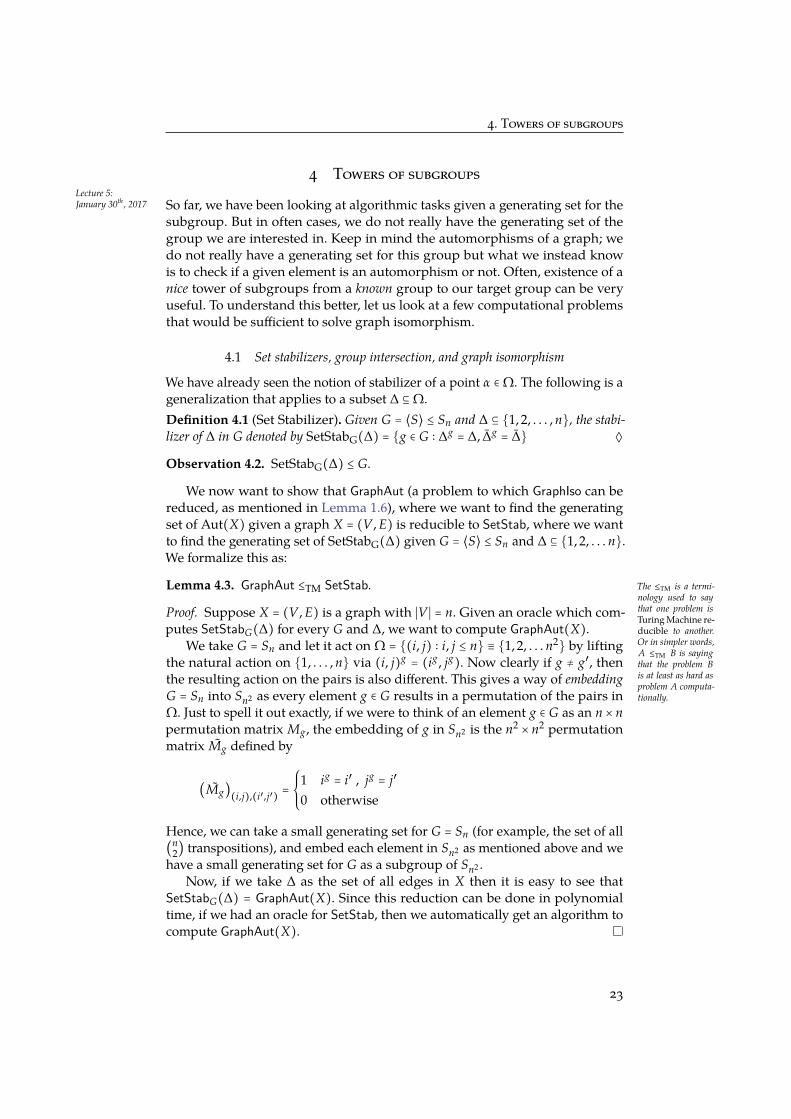
We take G = Sn and let it act on Ω = (i, j) ∶ i, j ≤ n ≡ 1, 2, . . . n2 by liftingthe natural action on 1, . . . , n via (i, j)g = (ig, jg). Now clearly if g ≠ g′, thenthe resulting action on the pairs is also different. This gives a way of embeddingG = Sn into Sn2 as every element g ∈ G results in a permutation of the pairs inΩ. Just to spell it out exactly, if we were to think of an element g ∈ G as an n × npermutation matrix Mg, the embedding of g in Sn2 is the n2 × n2 permutationmatrix Mg defined by
(Mg)(i,j),(i′,j′) =
⎧⎪⎪⎨⎪⎪⎩
1 ig = i′ , jg = j′
0 otherwise
Hence, we can take a small generating set for G = Sn (for example, the set of all(n
2) transpositions), and embed each element in Sn2 as mentioned above and wehave a small generating set for G as a subgroup of Sn2 .
Now, if we take ∆ as the set of all edges in X then it is easy to see thatSetStabG(∆) = GraphAut(X). Since this reduction can be done in polynomialtime, if we had an oracle for SetStab, then we automatically get an algorithm tocompute GraphAut(X).
23

4. Towers of subgroups
A problem very closely related to SetStab is the group intersection problem.The group intersection problem (which we’ll denote by GroupIntersect(S, T)) iswhere we are given G = ⟨S⟩ and H = ⟨T⟩ and we want ot find a generating setfor G ∩ H efficiently. The following lemma shows that this problem is in factequivalent to SetStab.
Lemma 4.4. SetStab ≡TM GroupIntersect. The notation ≡TMjust means that both≤TM and ≥TM holds.That is, if you cansolve one, then youcan solve the other aswell.
Proof. First, we show that SetStab ≤TM GroupIntersect. Suppose G ≤ Sn and∆ ⊆ 1, 2, . . . n. Given an oracle which computes GroupIntersect(H1, H2) forevery H1, H2 ≤ Sn, we want to compute SetStabG(∆).
Take H = ⟨(i j) ∶ i, j ∈ ∆ or i, j ∈ ∆⟩. Note that the size of the generating setis small. Now clearly, H is the set of all permutations on 1, 2, . . . , n elementswhich permute elements of ∆ within ∆ and that of ∆ within ∆. Hence it is easyto see that SetStabG(∆) = GroupIntersect(G, H)
Next, we show that GroupIntersect ≤TM SetStab. Suppose G, H ≤ Sn. Givenan oracle which computes SetStabG′(∆) for every G′ and ∆, we want to computeGroupIntersect(G, H).
Consider G′ = G × H which acts on Ω = (i, j) ∶ i, j ≤ n as (i, j)(g,h) =
(ig, jh). We note that there is a small generating set for G′ since it is generatedby (g, id) ∶ g ∈ S ∪ (id, h) ∶ h ∈ T where G = ⟨S⟩ and H = ⟨T⟩. Then for∆ = (i, i) ∶ i ≤ n, we see that (g, h) ∈ ⟨SetStabG′(∆)⟩⇔ ∀i, ig = ih ⇔ g = h. Thus,G ∩ H = ⟨g ∶ (g, g) ∈ SetStabG′(∆)⟩.
Both the reductions described above are achievable in polynomial time andhence we have the lemma.
4.2 Descending towers
Using Lemma 4.3 and Lemma 4.4 we have GraphAut ≤TM GroupIntersect. But inmany instances, knowing some additional properties about the groups wouldhelp us solve them efficiently. Much of this amounts to existence of some nicetowers and we formalize that notion below.
Lemma 4.5 (Descending nice towers). Given G = ⟨S⟩ ≤ Sn, if there exist G1, . . . , Gksuch that G = G0 ≥ G1 ≥ G2 ≥ ⋯ ≥ Gk = H for some target subgroup H and if:
• [Gi−1 ∶ Gi] ∶=∣Gi−1∣∣Gi ∣
= poly(n, ∣S∣) for all i ∈ [k].
• For any i ∈ [k], given a g ∈ Gi−1, there is an efficient algorithm to check if g ∈ Gi.
then we can efficiently compute T such that H = ⟨T⟩.3
However, in order to prove Lemma 4.5, it is enough to solve it for k = 1, sincewe can then use it repeatedly. Hence, we show:
Lemma 4.6. Let G = ⟨S⟩ and H ≤ G is a subgroup with [G ∶ H] = r = poly(n) that isrecognizable i.e there is an oracle which can test membership in H. Then, a generatingset for H can be computed efficiently.
3In more generality, if [Gi−1 ∶ Gi] ≤ r, it can be computed in time polynomial in n, ∣S∣ and r.
24

4. Towers of subgroups
Proof. We note that it is enough to find distinct coset representatives for H ≤ G,say R = a1, a2, . . . ar (i.e. G = ⊍r
i=1 ai H), as then Schrier’s Lemma (Lemma 3.6)says that a−1
i gaj ∶ ai, aj ∈ R, g ∈ S∩ H generates H. So, we look at an algorithmto find the distinct coset representatives for H.
Algorithm 15: FindCosetRepsInput : G = ⟨S⟩ ≤ SnOutput :The coset representatives of H in G
1 CR← id
2 repeat3 for each g ∈ S, ai ∈ CR do4 add gai to CR
// Check if gai was actually giving a new coset
5 for each aj ∈ CR do6 if a−1
j gai ∈ H then // via membership test in H7 remove gai from CR8 break out of for loop
9 until CR does not grow10 return CR
First, we note that G acts on Ω = a1H, a2H, . . . ar H by left multiplication.Further, the action is transitive, that is, given any ai H, for every ajH ∈ Ω, ∃g =
aja−1i ∈ G such that g acts on ai H to give ajH.Since [G ∶ H] = r, the orbit graph of G action on Ω has r vertices and is
connected as G acts transitively. Therefore, the above process discovers all thevertices of the orbit graph in poly(∣S∣, n, r) time.
4.3 Revisiting the group intersection problem
So now that we have proved Lemma 4.5, we revisit GroupIntersect problem insome special cases.Definition 4.7. Let G, H ≤ Sn. G is said to normalize H if for every g ∈ G and h ∈ H,ghg−1 ∈ H. ◊
For example, if H ⊴ G, then certainly G normalizes H just by the definitionof normality. But the above definition includes cases when H ⊴ K and G is somesubgroup of K (which may not contain H entirely).
Lemma 4.8. Given G = ⟨S⟩, H = ⟨T⟩ such that G normalizes H, then problemGroupIntersect(G, H) can be solved efficiently.
Proof. In order to use Lemma 4.5, we want to find a tower beginning in G andending in G ∩ H which satisfies the conditions of the lemma. Consider the mostnatural tower beginning at G, namely the stabilizer chain:
G ≥ G(1) ≥ G(2) ≥ . . . ≥ G(n) = id
25
4. Towers of subgroups
where G(i) consists of the permutations in G that do not move any of 1, . . . , i.From this, we get the tower
GH ≥ G(1)H ≥ G(2)H ≥ . . . ≥ G(n)H = H.
Note that these products G(i)H makes sense as G(i)H is indeed a group becauseG (and hence G(i)) normalizes H. From this, we can also obtain the tower G =
G ∩GH ≥ G ∩G(1)H ≥ G ∩G(2)H ≥ . . . ≥ G ∩G(n)H = G ∩ H.Clearly, thanks to Lemma 4.5, it is enough to show:
1. [G(i)H ∩G ∶ G(i+1)H ∩G] is small.
2. For every i and every g ∈ G(i−1)H ∩ G we should be able to check g ∈
G(i)H ∩G efficiently.
We first note that the membership test can be done efficiently. Indeed, forevery g ∈ G(i−1)H ∩G, we already know that g ∈ G and so it is enough to checkg ∈ G(i)H efficiently. Now this can be done using Algorithm 7 since we havea small generating set for G(i)H, namely Si ∪ T where Si a generating set ofG(i) (which we know how to obtain via successive stabilizer applications usingAlgorithm 4)
To check that [G(i)H ∩G ∶ G(i+1)H ∩G] is small, since [G(i) ∶ G(i+1)] is smalland G(i) normalizes H for every i, the following observations are enough:
1. H, K ≤ G are such that G normalizes H ⇒ [GH ∶ KH] ≤ [G ∶ K]
2. H, K ≤ G⇒ [G ∩ H ∶ K ∩ H] ≤ [G ∶ K]
The proofs of these two observations are left as an exercise∗. ∗ Would be a partof Problem Set 1 thatwould be coming upshortly.
We already know that [G(i) ∶ G(i+1)] ≤ n (why?) and hence the above twoobservations show that [G(i)H ∩G ∶ G(i+1)H ∩G] ≤ n as well. Thus, we indeedhave a nice tower and Lemma 4.5 lets us get a generating set for G ∩ H.
Next, we claim that if G, H are groups such that H◁◁ ⟨G, H⟩, then we cancompute GroupIntersect(G, H) efficiently. We formalize this as:
Lemma 4.9. Given G = ⟨S⟩, H = ⟨T⟩ such that H◁◁ ⟨S ∪ T⟩, GroupIntersect(G, H)
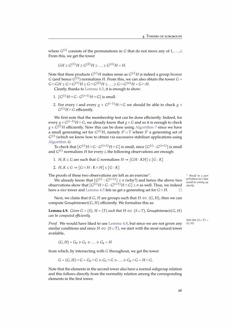
can be computed efficiently.Note that ⟨S ∪ T⟩ =⟨G, H⟩Proof. We would have liked to use Lemma 4.8, but since we are not given any
similar conditions and since H◁◁ ⟨S ∪ T⟩, we start with the most natural toweravailable,
⟨G, H⟩ = G0 ▷G1 ▷ . . .▷Gk = H
from which, by intersecting with G throughout, we get the tower
G = ⟨G, H⟩∩G = G0 ∩G▷G1 ∩G▷ . . .▷Gk ∩G = H ∩G.
Note that the elements in the second tower also have a normal subgroup relationand this follows directly from the normality relation among the correspondingelements in the first tower.
26

4. Towers of subgroups
Now we note that Gi ∩G normalizes Gi+1. Indeed, for g ∈ Gi ∩G, h ∈ Gi+1, wehave g−1hg ∈ Gi+1 due to the normal subgroup relations in the first tower. Thus,by Lemma 4.8, if we have a generating set for Gi ∩G, we have a generating setfor Gi+1 ∩G. Since we have a generating set for G = G0 ∩G, we can descend thischain and find a generating set for Gk ∩G = H ∩G, thus proving the lemma.
Lecture 6:February 3rd, 2017 In this lecture, equipped with Descending Nice Towers (see Lemma 4.5), we
proceed to tackle automorphism problems:
4.4 Solving an Automorphism Problem
The Coloured Graph Automorphism problem is a natural generalization ofthe general automorphism problem. In this problem, we are given a graphX and a colouring of the vertices and we want to output a generating set forthe group of automorphisms of X that respect the colours of the vertices. Theidea of mapping vertices of a degree only to vertices of the same degree isnicely encapsulated here by colouring all vertices of a degree by a single colour.Although this colouring would be respected by any automorphism, abstractingsuch properties to colours will be useful as we will see later in the lecture. Let’sfirst formally define coloured graph automorphism:Definition 4.10 (Coloured Graph Automorphisms). For a graph X = (V, E) on nvertices and a colouring of its vertices φ ∶ V → C, where C = 1, 2, . . . , n, the colouredautomorphisms of X, denoted by Autφ(X), is the following set of permutations:
Autφ(X) = σ ∈ Sym(V) ∶ (u, v) ∈ E⇐⇒ (σ(u), σ(v)) ∈ E and φ(v) = φ(σ(v)) .◊
Task: Given X, φ, find a generating set for Autφ(X).
If every vertex is coloured 1, this is just the automorphism problem. Alsonote that no matter what the colouring is, one can attach certain large gadgets(a unique gadget for each colour) to each vertex and remove the colours, thusreducing coloured graph automorphism to graph automorphism on a polyno-mially larger graph. Despite the equivalence of these two problems, we will nowsolve coloured graph automorphism for a certain class of colourings:
Bounded Colour Multiplicity Graph Automorphism: Given a graph X = (V, E)
on n vertices and a colouring of its vertices φ ∶ V → C such that ∀i ∈
C ∣φ−1(i)∣ ≤ b, find a generating set for Autφ(X).
Theorem 4.11. Bounded Colour Multiplicity Graph Automorphism can be solved inpoly(n, 2b2
) time.
Proof. We solve this problem using a quite intuitive descending nice tower.Notational warning: we call the elements of the tower G0, G1, G2 . . . Gk, but wewill sometimes add subscripts to these groups to better illustrate how Gt+1 isobtained from Gt. Before defining the tower, we introduce some more notation:Let Ω = V be the set that our groups act on. We split Ω into disjoint subsets
27

4. Towers of subgroups
based on the colours of the vertices:
Ω = ⊍i∈C
Ωi where Ωi = Φ−1(i)
Similarly, we split E into O(n2) sets based on the colours of the endpoints of theedges:
E = ⊍i≤j∈C
Ei,j where Ei,j = E ∩Ωi ×Ωj
As the first element of our tower, we take G0 = Sym(Ω1) × Sym(Ω2) ×⋯×
Sym(Ωn), the set of colour respecting permutations. Clearly Autφ(X) is a sub-group of G0 and we can construct a generating set for G0.
We incrementally approach Autφ(X) by ensuring that the permutations map(i, j) edges to edges (the permutations already respect colour, so they are mappedto (i, j) edges and then (i, j) nonedges would have to map to (i, j) nonedges) untilwe end up with only those colour respecting permutations that map edges toedges and nonedges to nonedges: Autφ(X). With this in mind, we take elementsfrom the set C ×C in any order, and we build a tower of length O(n2), whereGt+1
i−j is defined as follows:
Gt+1i−j = σ ∈ Gt ∶ (u, v) ∈ Ei,j ⇐⇒ (σ(u), σ(v)) ∈ Ei,j
It is easy to see that Gt+1i−j is a subgroup of Gt and to see that the last element of
the group is Autφ(X). We claim that the tower so defined is a descending nicetower. For this we need to show the following:
• Gt+1i−j is recognizable in Gt. This is easy to see, since we only need to check
that (i, j) edges map to edges.
• [Gt ∶ Gt+1i−j ] is small. We will show that it is in fact ≤ 2b2
.
To bound the number of cosets, consider g, g′ ∈ Gt. If g−1g′ ∈ Gt+1, then g′ = ghfor some h ∈ Gt+1 and so g and g′ lie in the same coset. Now we note that ifg(Ei,j) = g′(Ei,j) = E′, then g′ maps an element of Ei,j to an element of E′ and g−1
would map it back to Ei,j. Hence g−1g′ ∈ Gt+1 and so g and g′ are in the samecoset. By looking at the image of the action of g on Ei,j, we can now divide Gt
into equivalence classes such that any two elements in the same equivalenceclass lie in the same coset. Since each equivalence class corresponds to an E′
and E′ ⊆ Ωi ×Ωj, there are atmost 2b2equivalence classes and hence atmost 2b2
cosets.Now that we have shown that our tower is a descending nice tower we can
use Lemma 4.5 to solve Bounded Colour Multiplicity Graph Automorphism inpoly(n, 2b2
) time.
This result has some implications for graph automorphism. For example,if we had a graph in which there are atmost a constant number of vertices ofeach degree, we can find the automorphisms of that graph. However, a more
28

5. Divide and Conquer techniques.
promising problem to be solving is bounded degree graph automorphism, whichbounded colour multiplicity graph automorphism doesn’t seem to be helpingin.
5 Divide and Conquer techniques.
We will now introduce colour stabilizers and blocks, which we plan to use lateron in a divide and conquer algorithm aimed at tackling bounded degree graphisomorphism.Definition 5.1 (Colour Stabilizers). Suppose G acts on a coloured set Ω. Then, thecolour stabilizer of Ω, denoted by colourStabΩ(G) is defined as
colourStabΩ(G) = g ∈ G ∶ ag ∼ a ∀a ∈ Ω
where a ∼ b means that a and b are coloured with the same colour. ◊
5.1 Intransitive case
Note that if you are given a graph X = (V, E) and you define Ω as V × Vcoloured with two colours, red if α ∈ E and black otherwise, then it is clearthat colourStabΩ(Sym(V)) is just the set-stabilizer of the edges, which we knowis Aut(X). While we do not know how to find colourStab, we will see that itmight possible for this computation to be broken down into subproblems:
If G does not act transitively on Ω, let us split Ω into the connected compo-nents of its orbit graph: Ω = ⊍r
i=1 Ωi. We can then see that
colourStabΩ(G) = colourStabΩ1(colourStabΩ2(⋯ colourStabΩr(G)⋯))
We can compute this by first computing the innermost colourStabΩr(G) to getG′, then trying to solve colourStabΩr−1(G′), which might again be split intosubproblems. In the worst case, Ω is eventually split into singletons, so we willend up solving at most ∣Ω∣ instances of colourStab. Of course, we do not knowhow to solve colourStab yet, but this dreaming may prove useful.
5.2 Blocks
As it turns out, even if G acts transitively on Ω, it might still have some usefulstructure to exploit:Definition 5.2 (Blocks). ∆ ⊆ Ω is a block if for all g ∈ G, either ∆g = ∆ or ∆g ∩∆ =
∅. ◊
Trivial examples of blocks are singletons or the whole set Ω. A more infor-mative example is the automorphism group of a complete binary tree, in whichany subtree is a block. No automorphism can map a subtree so that its image ispartially within the subtree and partially outside.
Claim 5.3. Let G be a group with a transitive action on Ω. If ∆ ⊆ Ω is a block, then ∣∆∣
divides ∣Ω∣.
29

5. Divide and Conquer techniques.
Proof. Let α ∈ ∆. Since G acts transitively on Ω, take elements g1, g2, . . . , g∣Ω∣ suchthat Ω = αg1 , αg2 , . . . , αg
∣Ω∣. ∆gi and ∆gj are both of size ∣∆∣ since actions arepermutations. Furthermore ∆gi and ∆gj are either the same or disjoint (otherwise∆gi g
−1j would not be ∆ but would have a non-zero intersection with it). Since
these cover Ω, it follows that they tile Ω and hence the claim follows.
Definition 5.4 (Primitive Action). A transitive action of G on Ω is said to be primitiveiff there are no nontrivial blocks. ◊
Just like in the intransitive case, whenever the action contains non-trivialblocks, we want to reduce the problem somehow. But first, we’ll look at a fewcomputations tasks related to blocks.
Finding non-trivial blocksLecture 7:February 6th, 2017 Since we want to find such blocks when we’re stuck with a transitive action,
we’d want to solve the following computational task:
Task: Given G = ⟨S⟩ , α ∈ Ω, find the smallest non-singleton block containing α.
We begin with our problem of finding the smallest non-singular block con-taining α ∈ Ω, given G = ⟨S⟩ and α ∈ Ω. We can solve this problem if we can findthe smallest block containing both α and β for any β ∈ Ω (solving this problemfor all β ∈ Ω and then choosing the one that gives smallest block).
We will assume that the group G acts on Ω transitively. We make the follow-ing observation.
Observation 5.5. If αg = β and βg = γ, then any block containg α, β must contain γ.
Proof. Let ∆ be arbitrary block that contains α, β. Then we have β ∈ ∆g ∩ ∆(as αg = β). By the definition of block, this forces ∆g = ∆, which implies thatβg = γ ∈ ∆g = ∆.
The above observation gives us following algorithm to compute the small-est block containing both α and β. Construct a graph X = (Ω, E) with E =
(γ, δ) ∶ ∃g ∈ G such that (γ, δ) = (α, β)g.
Claim 5.6. The connected components of X form the block system generated by theminimum block ∆ containing α and β.
Proof. Although, this might look intuitively rather plain, let us be diligent andwork out a few details to establish the veracity of our claim. Say ∆ is the small-est block containing α, β. Let us say that Γ = ∆1, . . . , ∆m is the block systemgenerated by ∆.
1. If γ is in the connected component of X containing α, then it must* belongto ∆. Hence the connected component of X containing α is contained in * If β ∈ ∆ ∩ ∆g if
αg= β.the smallest block containing α, β.
2. Now, we need to show that the connected compnent Y containing α indeeda block. Consider any g ∈ G and observe that since Y is connected, so is Yg.*
30

5. Divide and Conquer techniques.
So, if Y ∩Yg ≠ ∅, then Y = Yg or else the fact that Y is a maximal connected *Why? Think aboutedges in Y.sub-graph of X would be contradicted.
We would now have an algorithm if only we could somehow find out all theedges in E. All we are given is a generating set S of G. How do we find out allpairs (γ, δ) = (α, β)g? This is precisely the orbit of (α, β) in the action of G onΩ ×Ω. Now we have a complete algorithm. Convince yourself.
Algorithm 16: MinimumBlockOfAPairInput : G = ⟨S⟩ ≤ Sn acting transitively, and α, β ∈ ΩOutput :The smallest block ∆ containing α, β.
1 Consider the action of G on Ω ×Ω via (γ, δ)g = (γg, δg). UsingAlgorithm 1 compute the orbit E of (α, β) in this action.
2 Construct the graph X = (Ω, E) where E is the set of all pairs in the aboveorbit computation.
3 return connected component ∆ of X that contains α, β.
Algorithm 17: MinimumBlockInput : G = ⟨S⟩ ≤ Sn acting transitively, and α ∈ ΩOutput :The smallest non-singleton block ∆ containing α
1 for β ∈ Ω ∖ α do2 ∆β ∶= MinimumBlockOfAPair(S, α, β)
3 Let ∆ be the smallest of the ∆βs.4 return ∆.
5.3 Block systems and structure forests
Finding non-trivial blocks, informally, allow us to work with smaller group aswe can think of each block as one element and group action between the blocks.We characterize this intution be defining Block System.Definition 5.7 (Block System). Given a G that acts transitively on Ω, and a block∆ ⊆ Ω, the block system generated by ∆ is a collection Γ = ∆1, . . . , ∆m thatpartition Ω, that is
Ω =m⊍i=1
∆i,
where each ∆i = ∆g for some g ∈ G. ◊
Say we found the smallest block ∆ and suppose this ∆ generates the blocksystem Γ = ∆1, . . . , ∆m. It is possible that a union of a few of these ∆is form alarge block (keep in mind the automorphisms of a complete binary tree). Thequestion now can be can we find the smallest subset of Γ such that the union ofthose blocks form a large block? Indeed we can. All we need to do is think of Gacting on Γ instead of Ω and use Algorithm 17 again. This allows us to build an
31
5. Divide and Conquer techniques.
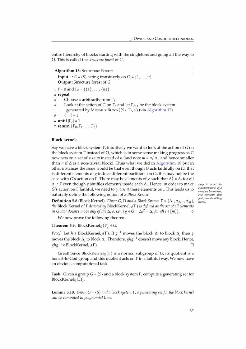
entire hierarchy of blocks starting with the singletons and going all the way toΩ. This is called the structure forest of G.
Algorithm 18: Structure ForestInput : G = ⟨S⟩ acting transitively on Ω = 1, . . . , nOutput :Structure forest of G
1 ` = 0 and Γ0 = 1 , . . . ,n.2 repeat3 Choose α arbitrarily from Γ`.4 Look at the action of G on Γ` and let Γ`+1 be the block system
generated by MinimumBlock(⟨S⟩ , Γ`, α) (via Algorithm 17)5 ` = ` + 16 until ∣Γ`∣ = 17 return Γ0, Γ1, . . . , Γ`
Block kernels
Say we have a block system Γ, intuitively we want to look at the action of G onthe block system Γ instead of Ω, which is in some sense making progress as Gnow acts on a set of size m instead of n (and note m = n/∣∆∣, and hence smallerthan n if ∆ is a non-trivial block). Thiis what we did in Algorithm 18 but inother instances the issue would be that even though G acts faithfully on Ω, thatis different elements of g induce different partitions on Ω, this may not be thecase with G’s action on Γ. There may be elements of g such that ∆g
i = ∆i for all∆i ∈ Γ even though g shuffles elements inside each ∆i. Hence, in order to make Keep in mind the
automorphisms of acomplete binary tree,and elements thatjust permute siblingleaves.
G’s action on Γ faithful, we need to quotient these elements out. This leads us tonaturally define the following notion of a Block Kernel.Definition 5.8 (Block Kernel). Given G, Ω and a Block System Γ = ∆1, ∆2, .., ∆m,the Block Kernel of Γ denoted by BlockKernelG(Γ) is defined as the set of all elementsin G that doesn’t move any of the ∆i’s, i.e., g ∈ G ∶ ∆i
g = ∆i for all i ∈ [m]. ◊
We now prove the following theorem.
Theorem 5.9. BlockKernelG(Γ) ⊴ G.
Proof. Let h ∈ BlockKernelG(Γ). If g−1 moves the block ∆i to block ∆j then gmoves the block ∆j to block ∆i. Therefore, ghg−1 doesn’t move any block. Hence,ghg−1 ∈ BlockKernelG(Γ).
Great! Since BlockKernelG(Γ) is a normal subgroup of G, its quotient is ahonest-to-God group and this quotient acts on Γ in a faithful way. We now havean obvious computational task.
Task: Given a group G = ⟨S⟩ and a block system Γ, compute a generating set forBlockKernelG(Ω).
Lemma 5.10. Given G = ⟨S⟩ and a block system Γ, a generating set for the block kernelcan be computed in polynomial time.
32

5. Divide and Conquer techniques.
Proof. We will do this by showing the existence of a ‘nice tower’ G = G0 ≥ G1 ≥
... ≥ Gm = H such that [Gi−1 ∶ Gi] is small and given g ∈ Gi−1, we can efficientlycheck if g ∈ Gi.
Let Gi = g ∈ G ∶ ∆gj = ∆j ∀j ≤ i. Note that Gi is SetStabGi−1(∆i). We have
seen that computing set stabilizer is hard . But here we know ∆i’s are block andwe will show this leads to polynomial time algorithm. Since ∆i’s are block soonly m distinct images of ∆i is possible and thus [Gi−1 ∶ Gi] ≤ m ≤ n. Also giveng ∈ Gi−1, it is easy to check if g ∈ Gi. This implies polynomial time algorithm forcomputing Gm i.e., BlockKernelG(Γ) (via Lemma 4.5).
Blocks and subgroups
We now try and understand when groups actions would have non-trivial blocks.The following theorem gives an exact characterization of this.
Theorem 5.11. Let G acts on Ω transitively. Then G’s action is primitive if and onlyif stabG(α) is a maximal strict subgroup of G.
Proof. (⇐): Suppose G’s action is not primitive. Therefore, there exists a non-trivial block containing α. Let ∆ be the smallest non-trivial block containing α.Then we have stabG(α) ≤ stabG(∆) ≤ G. Our goal is to show both of the inclusionis strict. Since ∆ is a non-trivial block so it must contain some β (β ≠ α). Letαg = β. Since ∆ is a block so g ∈ stabG(∆). But g /∈ stabG(α) (as it moves α). Thus,we have stabG(α) < stabG(∆).
For the second inclusion, we observe that G acts on Ω transitively but stabG(∆)
doesn’t (as it is a non-trivial block). This proves stabG(α) < stabG(∆) < G.
(⇒): Now assume there exists a H s.t. stabG(α) < H < G. We will show that∆ = αH (orbit of α on the action of H) is a non-trivial block. It suffices to showthat ∆ is indeed a block, and 1 < ∣∆∣ < ∣Ω∣.
It immediately follows from stabG(α) < H that ∣∆∣ > 1. From the Orbit Stabi-lizer theorem (Theorem 2.12), we have ∣∆∣ ⋅ ∣ stabG(α)∣ = ∣H∣ and ∣Ω∣∣ stabG(α)∣ =∣G∣. Also we have ∣ stabG(α)∣ = ∣ stabH(α)∣ and ∣H∣ < ∣G∣ (as stabG(α) < H < G).Thus, 1 < ∣∆∣ < ∣Ω∣.
The fact that ∆ is indeed a block is left as an easy exercise.
With this lemma, we can hope to find out the structure of groups whoseactions are primitive.
5.4 Sylow Theorems and p-groups
One instance of the above lemma that we’ll use shortly for bounded degreegraph isomorphism is the case when ∣G∣ is a power of a prime p. Such groupsare called p groups and there is a lot of theory about structure of p-groups. We’lltake an aside for now and look at the Sylow Theorems. We won’t be needing allof them in the course but they are good to know in any case.
Theorem 5.12 (Sylow’s Theorem). Let ∣G∣ = prm, such that gcd(m, p) = 1. Then
1. (Existence) There is a subgroup P ≤ G of size pr (p-sylow subgroup).
33

5. Divide and Conquer techniques.
2. (Relations) If P and Q are two p-sylow subgroups of G, then ∃g ∈ G, such thatgPg−1 = Q.
3. (Count) If np is the number of p-sylow subgroups of G, then np ≡ 1 mod p andnp∣m.
Proof. (1) Let Ω be the set of all subsets of size pr. Therefore, ∣Ω∣ = (prmpr ) ≢
0 mod p. Let G act on Ω via left multiplication, i.e., if S ∈ Ω then Sg = g ⋅α∣α ∈ S. Let Ω1, Ω2, .., Ωt be the orbits of Ω under the action of G. Therefore,Ω = Ω1 ∪ ..∪Ωt. One of the sets
S ∈ Ω is ourp-Sylow subgroup.What would be theorbit of S? Thesemust be preciselythe cosets and hencewe hope to find oneΩi of size exactly m.Now how do we dothat?
Since ∣Ω∣ ≠ 0 mod p, therefore there exists i ∈ [t] such that ∣Ωi∣ ≢ 0 mod p.Also note that ∣Ωj∣ ≥ m for all j since
⋃S∈Ωj
S = G.
as for any a, b ∈ G, there is a g ∈ G such that ga = b. This forces ∪S∈Ωj S to coverall of G and that is possible only if there are at least m elements in Ω as ∣S∣ = pr.
Let S be any set in Ωi and P be stabG(S). Claim is that ∣P∣ = pr. To see thiswe apply the orbit stabilizer theorem and get ∣P∣∣Ωi∣ = prm. Since ∣Ωi∣ ≥ m and∣Ωi∣ ≢ 0 mod p, we get ∣P∣ = pr.
(2) Let P be a p-sylow subgroup of G. Let Ω be the m left-cosets of P. LetΩ = a1P, a2P, .., amP. Suppose Q is another p-sylow subgroup of G. Let Q act onΩ via left multiplication, as (aiP)q = q ⋅ ai ⋅ P. Let Ω1, Ω2, .., Ωt be the orbits of Ωunder the action of Q. Therefore, we have∑i ∣Ωi∣ = m /≡ 0 mod p. By the orbit sta-bilizer theorem, each ∣Ωi∣ must divide pr. This implies that atleast one of Ωi (sayΩ1) must have size equal to 1. This means Ω1 = a1P and qa1P = a1P ∀q ∈ Q.This implies a−1
1 qa1 ∈ P for all q ∈ Q. So we get a−11 Qa1 = P.
(3) Let Q be a p-sylow subgroup of G. Consider the set of p-Sylow subgroups We didn’t do this inclass, but useful toknow.of G,
Ω = P1, . . . , Pnp .
Let us look at the action of G on Ω via Pqi = q−1Piq. We know from (2) that the
action is transitive. Hence in order to find ∣Ω∣. Hence we have that np ∣ ∣G∣. If wecould show that np ≡ 1 mod p, then it would also follow that np mod m.
Instead of G acting on Ω, we shall consider the action of a p-Sylow subgroupP via conjucation. But we have a smaller group P acting on Ω, we could end upwith a partition of Ω as orbits Ω = Ω1 ∪⋯∪Ωk. By the Orbit-Stabilizer Theorem As a bonus,
we also knowthat stabG(P) =
NormalizerG(P) =NP and hencenp = [G ∶ NP].
(Theorem 2.12), we know that ∣Ωi∣ divides ∣Q∣ = pr. We know that Q ∈ Ω, and isclear that its orbit is just Q. The goal would be to show every other orbit hassize at least p and this would show that ∣Ω∣ = np ≡ 1 mod p.
Take a P ≠ Q. We wish to show that the orbit of P cannot be P. What is thestabQ(P)? This precisely
stabQ(P) = q ∈ Q ∶ q−1Pq = P =∶ NormalizerQ(P).
34

5. Divide and Conquer techniques.
Again, by the Orbit-Stabilizer Theorem (Theorem 2.12), it suffices to show thatNormalizerQ(P) is a proper subgroup of Q. Observe that NormalizerQ(P) =
NormalizerG(P)∩Q. So the only way NormalizerQ(P) = Q is if it happens thatQ ⊆ NormalizerQ(P). But then Q and P are both p-Sylow subgroups sittinginside NormalizerG(P). Applying (2) to this means that Q = g−1Pg for someg ∈ NormalizerG(P), which is absurd as the very definition of the normalizerforces g−1Pg = P. Hence stabQ(P) < Q and hence the orbit of P must have sizebigger than 1. This forces every other orbit to have size that is a multiple of p.Therefore, np ≡ 1 mod p.
Lecture 8:February 10th, 2017andLecture 9:February 13th, 2017
Remember that we were trying to study the structure of groups that actprimitively on some set Ω. Suppose, ∣G∣ = pr and G acts faithfully, transitivelyand primitively, then what can we say about ∣Ω∣ and G? Using Theorem 5.11we conclude* that ∣ stabG(α)∣ = pr−1, which forces hence ∣Ω∣ = p. However, as * Why? Clearly,
you have not gonethrough ProblemSet 1.
G ≤ S∣Ω∣ since G acts faithfully, we must have r = 1. Hence, G = Cp, the cyclicgroup of order p. We’ll record this as an observation.
Observation 5.13. If G is a p-group acting faithfully, transitively and primitively ona set Ω, then G must be a cyclic group the order p and ∣Ω∣ = p.
5.5 Divide and conquer via blocks
Let us return to the transitive action of G on Ω, where Γ = ∆1, . . . , ∆m is a blocksystem and H = BlockKernelG(Γ). Let a1H, . . . , ar H be the set of cosets of Hin G. Now, let us generalize the concept of colourStabΩ(G), to replace G withany arbitrary set K as, colourStabΩ(K) ≜ g ∈ K ∣ ag ∼ a ∀a ∈ Ω. The followingis then immediate:
colourStabΩ(G) =r⋃i=1
colourStabΩ(ai H).
However, we must ask whether it is even sensible to efficiently ”get hold”of colourStabΩ(K), for an arbitrary K. After all, we have always been dealingwith large sets that were groups and hence one could hope for getting hold of asmall sized generating set. Fortunately, things don’t go astray if K happens to bea coset.
Lemma 5.14. If colourStabΩ(aH) is non-empty, then it is a coset of colourStabΩ(H).
Proof. Consider τ and σ in colourStabΩ(aH). Then, it is plain to see that τ−1σstabilizes colors, and as both τ and σ are members of aH, τ−1σ ∈ H.
Hence, we can specify colourStabΩ(aH) by giving a generator for colourStabΩ(H)
and an arbitrary coset representative.
Hence, if we are interested in solving the colour stabilizer for G, and if H ≤ G,we can recursively call colour stabilizer on each of the cosets of H in G andsomehow stitch the answers together. We’ll see this entire machinary in actionto see how we can solve the colour stabilizer on p-groups.
35

6. Colour Stabilizer for special groups
6 Colour Stabilizer for special groups
To begin with, we shall focus on the case when G is a p-group. At a later point,we would have to generalize to other structured groups but the following dis-cussions would have all the ideas.
p-ColourStabilizer: We are given as input G = ⟨S⟩ ≤ Sn, some permutationσ ∈ Sn and a set B ⊆ Ω that is a union of orbits . The goal is to compute To begin with,
B would just beΩ but we willneed this generalform in interme-diate steps of thedivide-and-conquer.
colourStabB(σG) ∶= π ∈ σG ∶ bπ ∼ b ∀ b ∈ B ,
where the output is expected as an ordered pair (π, T) for some π ∈ Sn andT ⊆ Sn such that colourStab(σG) = π ⋅ ⟨T⟩ (thanks to Lemma 5.14).
6.1 If G is not transitive
If B is a union of orbits, say, B = Ω1 ∪⋯∪Ωr, then we use
colourStabB(σG) = colourStabΩ1(colourStabΩ2(⋯ colourStabΩr(σG)⋯))
6.2 If G is not primitive
If G is not primitive, we shall find a block system Γ and the associated blockkernel H ⊴ G and if G = a1H ∪⋯∪ ar H then
colourStabB(σG) =r⋃i=1
colourStabB(σai H).
We can try to compute each of the r terms on the RHS and combine them together.There are a few issues with this that need to be addressed:
1. We do not know how large r is. If r is too large, then there would be toomany recursive calls.
2. If each of the recursive calls on the RHS return some πi, Ti such thatcolourStabB(σai H) = πi ⟨Ti⟩, how are we supposed to combine them to-gether to a single π, T?
For the first issue, it is important that we make H as large as possible so thatr is as small as possible. For this, it makes sense to take the block system at thehighest level of the structure forest (Algorithm 18). So let’s assume that Γ is thatblock system. What can we say about ∣Γ∣ and r in that case? Observe that G/Hacts transitively, faithfully and primitively on Γ! Hence, by Observation 5.13,G/H = Cp and ∣Γ∣ = p. Hence, r = [G ∶ H] = p. This solves the first issue.
As for the second issue, the following lemma tells us how to paste the differentrecursive calls together.
Lemma 6.1. Let ⟨T⟩ = H ≤ G and suppose a1H ∪⋯ ∪ ar H is a coset of G. ThenS = ⟨T ∪ a−1
1 ai ∶ i = 2, . . . , r⟩ and a = a1 generate the coset given by a1H ∪⋯∪ ar H.
36

6. Colour Stabilizer for special groups
Proof. Exercise.
This lemma essentially solves the second issue. Each recursive call wouldreturn some πi, Ti (if non-empty) for each i = 1, . . . , r. Firstly, observe that⟨Ti⟩ = colourStabB(H) for all i so we might as well have a single T. Then, anapplication of the above lemma tells us how to paste the different cosets together.
We now write the entire algorithm for colour stabilizer for general groups(which may not be efficient for general groups as we may not have an analogueof Observation 5.13 for general groups) that is guaranteed to be efficient in thecase of p-groups.
Algorithm 19: ColourStabInput : G = ⟨S⟩ ≤ Sn, a permutation σ ∈ Sn and a union of orbits B ⊆ ΩOutput :π, T such that colourStabB(σG) = π ⟨T⟩
1 if G is “small” then2 Enumerate all the elements of G and solve colourStabΩ(σG) by
brute-force.3 return computed colour stabilizer.
4 if G does not act transitively on B then5 Break B into orbits Ω1, Ω2, . . . , Ωk
6 return colourStabΩ1(colourStabΩ2(. . . colourStabΩk(σG)⋯))
7 else if G does not act primitively then8 Compute the structure forest of G using Algorithm 18. Let Γ be the
block system at the highest level of the structure forest9 Compute a generating set U for H = BlockKernelG(Γ).
10 Compute a1, a2, . . . ar, a set of representatives of H in G11 for i = 1, . . . , r do12 Compute the colour stabilizer of σai H recursively as
bi, T = ColourStab(U, σai, B)
13 return b1, T ∪ b−11 b2, b−1
1 b3, . . . b−11 br
14 else// Want to set ‘‘small’’ in line 1 appropriately so that
we never get here.
15 return Fail
In the above algorithm, depending on the group we are working with, weneed to appropriately assign the meaning to “small” in line 1. If the group Gis from some structured class, we want this to be an upper bound of the sizeof any primitive, transitive group from this class. For the case of p-groups, thisvalue would just be p (Observation 5.13).
Theorem 6.2. If G = ⟨S⟩ ≤ Sn is a p-group, if “small” in line 1 is set to p thenAlgorithm 19 always outputs the colour stabilizer in time poly(n, p, ∣S∣) .
Proof. Let us get a sense of the number of recursive calls and the size of eachof those instances. Say ∣B∣ = m and let T(m) be the time taken to compute
37

7. Graph isomorphism for bounded degree graphs
colourStabB(G). If G does not act transitively on B, then we decompose B intoorbits. Say B = Ω1 ∪⋯Ωt and let mi ∶= ∣Ωi∣. Once we have these orbits, we thencompute the colour stabilizer in each of these orbits.
Each such recursive call would then construct the highest level block systemfrom the structure forest of Ωi. Let Γi be the highest level block system of Ωi andlet Hi be the block kernel. Since G/Hi acts transitively, primitively and faithfully*on Γi, we know that ∣Γi∣ = p and [G ∶ Hi] = p. Hence, if G = ai1Hi ∪⋯∪ aipHi, for * Why faithful?
each i, then if we can compute colourStabΩi(σaijHi) for each i = 1, . . . , t and j =1, . . . , p, we can stitch together a generating set for colourStabB(σG) with polyno-mial overhead. Hence, if T′(mi) is the time for computing colourStabΩi(σaijHi),then
T(m) ≤ pT′(m1)+⋯+ pT′(mt)+poly(n, m, ∣S∣).
Now comes the key observation: Each Hi stabilizes the blocks in Γi and hencethe orbits of Hi are of size at most ∣Ωi∣ /p as Hi never takes elements of one blockto another. Therefore, if Γi = Ωi1, . . . , Ωip (and recall ∣Ωi∣ = mi/p) we have
colourStabΩi(σaijHi) = colourStabΩi1(⋯ colourStabΩip(σaijHi)⋯)
Ô⇒ T′(mi) ≤ pT(mi/p)+poly(n, m, ∣S∣).
Putting it all together,
T(m) ≤ p2 (T(m1/p)+⋯+ T(mt/p))+poly(n, m, ∣S∣).
where ∑mi = m. Solving this recurrence shows that the time taken by the algo-rithm is poly(n, m, ∣S∣).
7 Graph isomorphism for bounded degree graphs
We have already seen that graph isomorphism and graph automorphism areequivalent (Lemma 1.6). In fact, it suffices to get a generating set for the set ofautomorphisms that fixes an edge.
Aute (X = (V, E)) = σ ∈ Sym(V) ∶ σ(e) = e and (u, v) ∈ E⇔ (σ(u), σ(v)) ∈ E
We stress that it is possible that a σ ∈ Aute(X) swaps the two end-points of e butall we insist is that the edge e is mapped to the same edge (and end-points couldpossibly be swapped).
Lemma 7.1. GraphIso reduces to the problem of computing a generating set for Aute(X).
Proof. By picture:
38

7. Graph isomorphism for bounded degree graphs
X Y Z
e
It is also worth noting that the above reduction also maintains the maximaldegree of the graph X (unless X has maximal degree at most 2 which is just aset of cycles and paths).
The general road-map would be the following.
• Step 1: Structural properties - Prove some structural properties of thegroup Aute(X) when X is a bounded degree graph.
• Step 2: Reduction to colour stabilizers - Reduce the task of computing agenerating set of Aute(X) to colourStab on such structured groups.
• Step 3: Solving colourStab - Show that colourStab of such structured groupscan be solved in polynomial time.
We shall first look at graph isomorphism for the class of degree 3 graphs,also called trivalent graphs. These would have all of the crucial ideas in Luks’algorithm for bounded degree graph isomorphism.
7.1 Trivalent Graphs
Assume without loss of generality that X is a connected trivalent graph (if not,we have to work with each connected component, etc.). The goal is to get agenerating set for Aute(X). We shall do that incrementally and in the processprove some structural properties of the automorphism group, as well as seehow to get a generating set for it. The idea is to discover the remaining edges inorder of their ”distance” from e, and use induction on the chain of sub-graphs,denoted by Xi, that arise.
Formally, let Xi consist of vertices that are reachable from one of the twoend points of e by a path of length at most i, and the edges in Xi would be allthose edges whose distance from e is at most i, i.e. there is a path of length atmost i containing that edge and e. The following picture is an example of theseintermediate graphs.
39

7. Graph isomorphism for bounded degree graphs
e
X
e
X0
e
X1
e
X2
e
X3 = X
We first proceed to Step 1 of the above outline which is to prove a structuralresult about Aute(X) in the case when X has degree at most 3. We will prove It is one of those
results where thestatement andthe proof are bothequally amazing.
the following amazing result by Tutte.
Theorem 7.2 (Tutte). If X is a connected trivalent graph, then Aute(X) is a 2-group,i.e., ∣Aut(X)∣ = 2k. What happens if X is
not connected?
Proof. We shall prove by induction on r that Aute(Xr) is a 2-group. In the caseof X0, which consists of a single edge, the claim is true as Aute(X0) consists ofjust two elements — the identity and the swap of the two end points of e. Nowassuming that Aute(Xr) is a 2-group, we wish to show that Aute(Xr+1) is alsoa 2-group. Informally, we shall show that the new elements, vertices or edgesso discovered, either reduce or increase the size of Aute(Xr+1) by a factor of 2j
compared to Aute(Xr).Let Gr = Aute(Xr), and let Vr be the set of vertices in Xr. We already have the
claim for r = 0. For r > 0, let us define a function φr ∶ Gr → Gr−1. This is just theprojection map, i.e., it ignores the action of Gr on Vr ∖Vr−1 as any e-preservingautomorphism of Xr induces an automorphism of Xr−1.* It is easy to see that φr * Any g in Gr
must permute Vr−1within itself. Why?is therefore a homomorphism and hence we have:
∣Gr ∣
∣ker(φr)∣= ∣ Im(φr)∣.
So, if we demonstrate that ∣ker(φr)∣ is a 2-group, we would have establishedthe theorem because by the inductive hypothesis, ∣Gr−1∣ is a 2-group, and henceIm(φr) ≤ Gr is a 2-group.
Let us now articulate on ker(φr) = g ∈ Aute(Xr) ∣ φr(g) = id on Vr−1. Wenow wish to know what the elements of Aute(Xr) whose action on Xr−1 is justidentity. For this purpose, for a vertex a ∈ Vr ∖Vr−1, define the neighbourhoodN(a) = b ∈ Vr−1 ∶ a, b ∈ Er.
Call distinct a and b twins* if N(a) = N(b), and distinct a, b and c triplets if * What else?
N(a) = N(b) = N(c). ∣N(a)∣ ≤ 3 and there are no triplets as the graph is trivalent.
40

7. Graph isomorphism for bounded degree graphs
Hence, the vertices in Vr ∖Vr−1 can be partitions into twins and single children.As, any g ∈ ker(φr) is an automorphism that fixes Vr−1, its action on the setVr ∖Vr−1 may only be that of swapping twins. Furthermore, any permutationwhich fixes Vr−1 and swaps twins is a member of ker(φr).** Thus, ker(φr) is ** Why? Ahh! the
edges between thevertices of Vr ∖Vr−1are not present in Er ;they only show up inEr+1.
generated by twin swaps, and hence, it is a 2-group.
An alternateproof by UmaGirish was thatany g ∈ ker(φr)
satisfies g2= id.
This is easy to checkand immediatelyimplies ker(φr) is a2-group.
For every r and every vertex v, let Xr, Gr, N(v) be as defined in the aboveproof. We note that the proof actually gives us an algorithm to find a generatingset for ker(φr).
Algorithm 20: Kernels between successive layersInput : Xr, Xr−1Output : T such that ⟨T⟩ = ker(φr)
1 T = ∅
2 For every v ∈ Vr ∖Vr−1, find N(v).3 Partition Vr ∖Vr−1 into twins and single children.4 for each pair of twins v, v′ ∈ Vr ∖Vr−1 do5 Add the transposition (v, v′) to T.6 return T
Now the road map to compute the generating set for Aute(X) would also bean inductive procedure of starting from X0 and slowly building a generating setfor the e-preserving automorphisms of larger Xis. Suppose we have a generatingset for Gr−1 = Aute(Xr−1). The following would be our strategy.
1. We shall use the map
φr ∶ Gr → Gr−1
and first construct the generating set for ker(φr) = ⟨K⟩ via Algorithm 20.
2. Recursively find a generating set for Im(φr). Note that Im(φr) consistsof precisely the automorphisms of Xr−1 that can be extended to Xr. If wecould compute a generating ⟨T⟩ = Im(φr), then for each g ∈ T let g be anextension of g to an automorphism of Xr. Let T = g ∶ g ∈ T. Then, K ∪ Tgenerate Gr as in essense this includes a generating set for a subgroup(ker(φr) ≤ Gr) and also its coset representatives (lifts of Im(φr)).
So now, the only thing left to do is to find a generating set for Im(φr) givenGr−1. To do that we shall show that Im(φr) is a suitable colour stabilizer of Gr−1.Since we know from Theorem 7.2 that Gr−1 is a 2-group, we can use Theorem 6.2to solve the colour stabilizer in polynomial time.
If σ ∈ Gr, then note that N(σ(v)) = σ(N(v)). In words, this is just stating thatthe neighbours of v must be mapped to the neighbours of σ(v). Since we areworking with a trivalent graph, N(v) is some subset of Xr−1 of size at most 3.Define
A = subsets of Vr−1 of size at most 3 .
41

7. Graph isomorphism for bounded degree graphs
Suppose a ∈ A such that there are v, v′ ∈ Vr ∖Vr−1 such that N(v) = N(v′) = abut b ∈ A such that there is only one v′′ such that N(v′′) = b, then note that noσ ∈ Gr can map a to b. Hence it makes sense to define the following subsets.
A1 = a ∈ A ∶ ∣N−1(a)∣ = 1
A2 = a ∈ A ∶ ∣N−1(a)∣ = 2
A = u, v ∈ A ∶ u, v ∈ Xr ∖Xr−1
If we were to consider the action of Gr on A via the natural lift, then clearly anyσ ∈ Gr must stabilize A1, and A2 and A. Turns out, the converse is also true.Lemma 7.3. Let σ ∈ Gr−1 such that σ stabilizes A1, A2 and A. Then σ can be extendedto an automorphism of Xr.Proof. The edges in Xr ∖Xr−1 are of three kinds:
• edges present in Xr−1,
• edges connecting a vertex in Vr−1 to a vertex in Vr ∖Vr−1,
• edges connecting two vertices in Vr−1, but was not present in Xr−1.The first kind of edges are of course preserved as σ ∈ Gr−1. The third kind of
edges are also preserved by σ as we are given that σ stabilizes A. We only needto ensure that second kind of edges are preserved by σ as well.
This is sort of immediate once we write things down properly. Considerlisting all the vertices in Vr ∖Vr−1 on the left and all elements of A on the right.Imagine connecting each v on the left with the a = N(v) on the right. Justnaturally extend σ to the vs by following these connections to the left. Forinstance, if σ(a) = σ(a′) and N−1(a) = v and N−1(a′) = v′, then extend σ bymappign v to v′. If σ(a) = σ(a′) and N−1(a) = v1, v2 and N−1(a′) = v′1, v′2,then extend σ by mapping v1 to v′1 and v2 to v′2 (or vice-versa; both would bevalid extensions but we just need one). This therefore preserves all edges betweenVr−1 and Vr ∖Vr−1. Hence σ can indeed be extended to an automophism of Xrand hence σ ∈ Im(φr).
Since we have solved colourStabΩ(G) for G which are p-groups, considerthe following algorithm to find the generating set for Im(φr) given Gr−1. Notethat since we are working with trivalent graphs, Gr−1 is a 2-groupfor every r byTheorem 7.2 and hence we can compute colourStabΩ(Gr−1) for any Ω.
Algorithm 21: Image between successive layersInput : Gr−1 = ⟨S⟩ , Xr, Xr−1Output : T such that ⟨T⟩ = Im(φr)
1 Consider the action of G on A = subsets of Vr−1 size at most 3.2 Define A = (u, v) ∈ Xr ∖Xr−1 ∶ u, v ∈ Vr−1.3 Define A1 = a ∈ A ∶ N(v) = a for exactly one v ∈ Vr.4 Define A2 = a ∈ A ∶ N(v) = a for exactly two v s ∈ Vr.5 Colour elements of (A1 ∩ A), (A1 ∖ A), (A ∖ A1), A2 and
A ∖ (A1 ∪ A2 ∪ A) with different colours.6 return colourStabA(Gr−1)
42
7. Graph isomorphism for bounded degree graphs
As mentioned earlier, once we obtain a generating set T for Im(φr), we lifteach of its elements to form T, add to it the generating set for ker(φr) and weget a generating set for Gr.
Repeating this for r = 1, . . . , n we eventually have Xr = X and thus a generat-ing set for Aute(X). Hence we have completed the following theorem.
Theorem 7.4 (Luks). Graph isomorphism for trivalent graphs can be solved in deter-ministic polynomial time.
7.2 Generalizing to higher (but bounded) degree graphs
Let us go through the motions again for graphs of degree bounded by d (think ofd = 100 or something). Once again, let us consider the layered graph X0, X1, . . .,and let Gr = Aute(Xr) and φ ∶ Gr → Gr−1 is the natural projection map. Previously,we first showed that the kernel of φr was a 2-group and that enabled us toinductively show that Aute(Xr) is a 2-group. However, this need not be the casehere. Nevertheless, the kernel is still a pretty structured group.
Structure of ker(φr)
As earlier, we shall say that v1, . . . , vt ∈ Vr ∖Vr−1 are identical siblings if N(v1) =
⋯ = N(vt). Note that t < d, for the same reasons that in a trivalent graph we can-not have triplets. The following is a natural generalization to obtain a generatingset for ker(φr) and the proof is straightforward.
Lemma 7.5. Let Vr ∖Vr−1 = T1 ⊍⋯⊍Tk be a partition of Vr ∖Vr−1 into sets of identicalsiblings. Then,
ker(φr) = Sym(T1)×⋯× Sym(Tk).
This isn’t quite as nice as a 2-group but nevertheless what we do know isthat ∣Ti∣ ≤ d − 1 which for us is a constant. So in some sense, ker(φ) has made asa combination of small groups. This is formalized by the notion of compositionfactors and we briefly describe this now.
Groups with bounded composition factors
Definition 7.6 (Bounded composition factors). A group G is said to have composi-tion factors bounded by d, denoted by G ∈ Bd if there is a normal series
G = G0 ▷G1 ▷⋯▷Gr = id
such that Gi/Gi+1 is isomorphic to a subgroup of Sd. ◊
If K = Sym(T1)×⋯× Sym(Tr) with ∣Ti∣ < d, then K ∈ Bd as
K = K0 ▷K1 ▷⋯▷Kr
where Ki = Sym(Ti+1)×⋯×Sym(Tr) and successive quotients are just Sym(Ti) ≤
Sd. Hence, ker(φr) ∈ Bd.
43

7. Graph isomorphism for bounded degree graphs
The class Bd have some very useful properties that we will state withoutproof.Lemma 7.7. If G ∈ Bd and H ≤ G, then H ∈ Bd.
Lemma 7.8. If N ◁G and if N ∈ Bd and G/N ∈ Bd, then G ∈ Bd.
With these two lemmas, we have an analogue of Tutte’s theorem in thissetting.Lemma 7.9. Gr = Aute(Xr) ∈ Bd.
Proof. As in Theorem 7.2, we shall prove this by induction. Consider the mapφr ∶ Gr → Gr−1. We know that Gr/ker(φr) ≅ Im(φr) ≤ Gr−1. By Lemma 7.7 andLemma 7.8, it follows that G ∈ Bd.
Great! We know some structural result about the groups we are workingwith.
Computing a generating set for Im(φr)
As earlier, we can let A be the set of subsets of Vr ∖Vr−1 of size at most d, anddefine sets A1, . . . , Ad−1 as
Ai = a ∈ A ∶ ∣N−1(a)∣ = i
and
A = u, v ∈ A ∶ u, v ∈ Xr ∖Xr−1 .
As in Lemma 7.3, any σ ∈ Gr−1 that stabilizer the above sets (when Gr−1 is actingon A) can be extended to a σ ∈ Gr.
We still however need to solve the colour stabilizer problem. For that, it wasimportant to know that any transitive, faithful and primitive p-group must besmall. Fortunately, there is an analogue of that for Bd which again we shall statewithout proof.Theorem 7.10 (Babai, Cameron, Palfy). There is an absolute constant c > 0 suchthat if G ∈ Bd act faithfully, transitively and primitively on a set Ω of size n then,∣G∣ ≤ O(ncd).
With this result, it is relatively straightforward to check that the colour stabi-lizer problem on groups in Bd can be solved efficiently.Theorem 7.11. Let G = ⟨S⟩ ∈ Bd acting on Ω of size m. Given S, a σ ∈ Sm and B ⊆ Ω,a generating set for colourStabB(σG) can be computed in deterministic poly(∣S∣, md)
time.
With this theorem, it follows that we can compute the generating set forIm(φr) in poly(nd2
) time (since G is now acting on A which has size m = nd,and the colour stabilizer algorithm takes time poly(md) = nO(d2
)). Thus puttingeverything together, we get the following theorem.Theorem 7.12 (Luks). Graph isomorphism for graphs of degree at most d can be solvedin deterministic nO(d2
) time.
44

8. General graph isomorphism
8 General graph isomorphismLecture 10:February 20th, 2017andLecture 11:February 24th, 2017
In the previous lecture, we have seen algorithms to solve the Graph Isomorphismfor restricted graphs like Bounded degree graphs and Trivalent graphs. In thislecture, we will see an algorithm due to Babai, Luks and Zemlyachenko whichruns in time nO(n2/3
). Note that the naıve algorithm runs in time n! ≈ nn.
8.1 Colour Refinements
The natural thing to do for solving Graph Isomorphism is to break up the verticesinto groups which are distinct in some way there by reducing the search space.We can think of this grouping as a colouring of the graphs. One way of groupingvertices in a graph is according to their degree because in any Isomorphismbetween X and Y, degree d vertices in X can only be mapped to degree d verticesin Y. We can further extend this argument and say neighbours of degree dvertices in X can only be mapped to neighbours of degree d vertices in Y andso on. This idea is used most of the time in practice. The Weisfeiller Lehmanrefinmenet process, which we see below, formalizes this idea.
Weisfeller-Lehman colour refinement
Let’s assume we have a colouring χ ∶ V → [k] to begin with. This could be justassigning the degree of each vertex as its colour, or even the trivial colouring.The following is a way to attempt to refine the colouring χ ∶ V → [k] to a newcolouring χ′ as follows:
• On each vertex v, set its colour as (χ(v); d1, . . . , dk) where where di is thenumber of neighbours of v that are given colour i by χ.
• Since the graph has at most n vertices, there can be at most n distinctvectors as colours. Re-index them using [k′] for a suitable k′.
This will indeed be a refinement of the previous colouring in the sense that ifχ′(v) = χ′(u) Ô⇒ χ(v) = χ(u). By repeating the above process, at some pointthere would be no further refinement in the colouring. We shall refer to this asthe WL process, where we start with a given colouring χ and keep refining untilthe colouring stabilizes.
When we are given two graphs X and Y that we need to check if they areisomorphic, we can simultaneously run the WL process on both graphs startingwith the colouring by degree. If we ever notice a discrepancy (that is, X hasmore 1 coloured vertices than Y), we immediately know that the graphs are notisomorphic. However, we might still have non-isomorphic graphs that end upwith the same WL refinements. Here is an example:
45

8. General graph isomorphism
X doesn’t have 5 cycles Y has a 5 cycle
So whenever the WL process gets stuck, we need to force progress in someway. This is done by what is called individualisation where you pick an arbitraryvertex v ∈ X and give it a completely fresh colour. This way, the WL processwould hopefully refine the colours further. The issue now of course is that wedo not know what the correct image of v is in the graph Y – which vertex of Ymust be coloured by this new colour? We know, if they are indeed isomorphic,then this must be one of the vertices of Y that had the same (previous) colour ofv. We shall try out all possibly candidates.
Thus, every time we individualize a vertex, we make the colours more refined,but we pay a multiplicative cost of (potentially) n we we need to try out allpossibilities of this individualized vertex in Y. But here is a heuristic that we canattempt.
Algorithm 22: GraphIso WL+Ind HeuristicInput :Graphs X and Y on n-vertices
1 Start with χ(v) = deg(v) for every v ∈ X and Y.2 Pairs = (X, Y)
3 repeat4 if Pairs is empty then5 return No6 for (X, Y) ∈ Pairs do7 Run the WL process in parallel on both X and Y. If there is is every
a discrepency observed, remove (X, Y) from Pairs.8 Pick a vertex v ∈ X and individualize v, and call this new coloured
graph Xv.9 For every u ∈ Y, let Yu be the graph where u is given the same new
colour.10 In Pairs, replace (X, Y) with (Xv, Yu) ∶ u ∈ Y.
11 until all graphs in Pairs become “nice”12 Run the Graph Isomorphism for “nice” graphs for every (X, Y) in Pairs
and return Yes if any of them is an isomorphic pair.
The ideal scenario is when we only have to individualize a few vertices andwe end up with a situation where we know how to solve graph isomorphism.One example could be the setting where all the colour classes are small. In thatcase, we can use the bounded colour multiplicity algorithm that we have seenearlier. Unfortunately, this approach doesn’t work as there are graphs wherewe need to individualize far too many vertices before the WL process results in
46

8. General graph isomorphism
bounded colour class sizes.Turns out if we work with a new notion called generalized colour valence
instead colour class size, then we can hope to reach this situation with fewindividualization operations.Definition 8.1. Generalized colour valence Let X = (V, E) be a graph and C1, . . . , Cmbe a colouring of V. Define the generalized colour valence for a vertex v and a colourclass Ci as
degi(v) ∶= min# neighbours
of v in Ci,
# non-neighboursof v in Ci
.
In words, either v has at most degi(v) neighbours or non-neighbours in Ci.We shall denote by deg(X) the maximum degi(v) over all possible v, i. ◊
The key point about this definition is the following theorem that we shalldefer to the end of this section.
Theorem 8.2. Graph Iso for graphs with gcd ≤ d can be solved in nO(d2) time.
The following crucial theorem tells us that by isolating a few vertices in theWL algorithm we end up with a graph with small generalized colour valence.
Theorem 8.3 (Zemlyachenko). For any X on n vertices and 1 ≤ d ≤ n , we can find atmost 4n/d vertices to individualize such that the WL refinement stabilizes to a colouringwhere deg(X) ≤ d.
With the above two theorems, the main result of this lecture is immediate.
Theorem 8.4 (Babai,Luks). Graph Iso can be solved in nO(n2/3) time.
Proof. From Theorem 8.3, obtain a colour refinement which isolates at most 4n/dvertices and leaves a colouring such that deg(X) ≤ d. For every vertex that isindividualized, try out all possible choices in the other graph. For each suchpair, check if the two graphs are isomorphic using the algorithm guaranteedby Theorem 8.2. The over all running time of the algorithm is poly(n4n/d ⋅ nd2
).By optimising over d and choosing d = n1/3 we get the running time to benO(n2/3
).
All that’s left to do is prove Theorem 8.2 and Theorem 8.3.
8.2 Reducing to the bounded generalized colour valence case
This section shall be devoted to Zemlyachenko’s trick (Theorem 8.3), and thisfollows from the following lemma.
Lemma 8.5. Given a graph X and a colouring such that deg(X) ≤ D. Then by doingthe WL process + individualizing step at most 2n/D times we end up with a colouringsuch that deg(X) ≤ D/2.
Proof. We’ll run the following process.
1. Run the WL process.
47
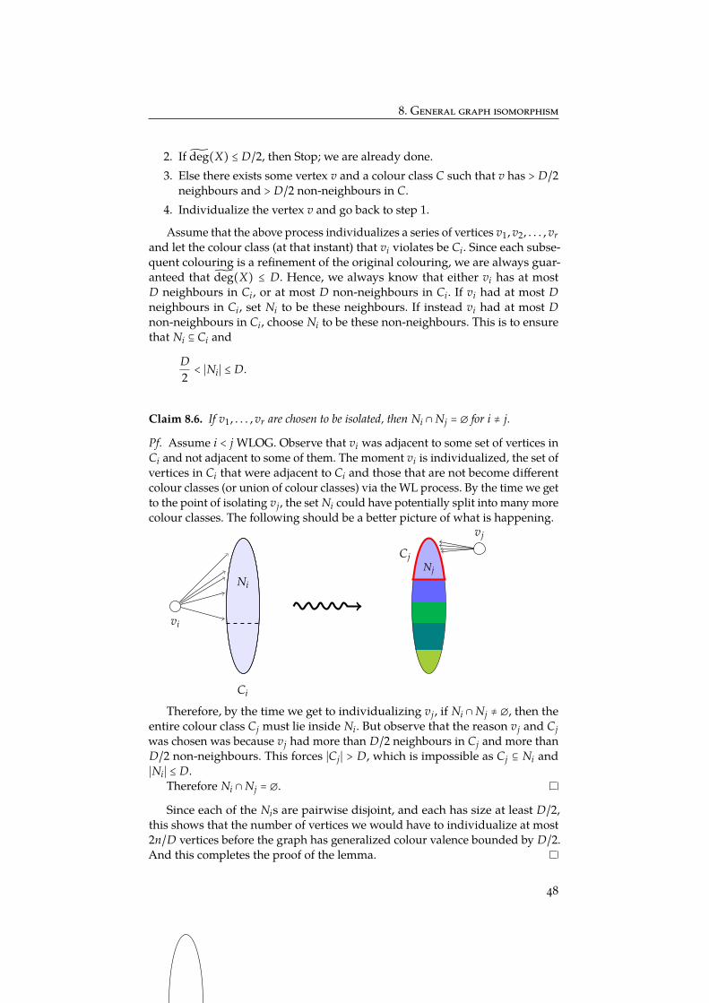
8. General graph isomorphism
2. If deg(X) ≤ D/2, then Stop; we are already done.3. Else there exists some vertex v and a colour class C such that v has > D/2
neighbours and > D/2 non-neighbours in C.4. Individualize the vertex v and go back to step 1.
Assume that the above process individualizes a series of vertices v1, v2, . . . , vrand let the colour class (at that instant) that vi violates be Ci. Since each subse-quent colouring is a refinement of the original colouring, we are always guar-anteed that deg(X) ≤ D. Hence, we always know that either vi has at mostD neighbours in Ci, or at most D non-neighbours in Ci. If vi had at most Dneighbours in Ci, set Ni to be these neighbours. If instead vi had at most Dnon-neighbours in Ci, choose Ni to be these non-neighbours. This is to ensurethat Ni ⊆ Ci and
D2< ∣Ni∣ ≤ D.
Claim 8.6. If v1, . . . , vr are chosen to be isolated, then Ni ∩ Nj = ∅ for i ≠ j.
Pf. Assume i < j WLOG. Observe that vi was adjacent to some set of vertices inCi and not adjacent to some of them. The moment vi is individualized, the set ofvertices in Ci that were adjacent to Ci and those that are not become differentcolour classes (or union of colour classes) via the WL process. By the time we getto the point of isolating vj, the set Ni could have potentially split into many morecolour classes. The following should be a better picture of what is happening.
vi
Ci
Ni
Cj
vj
Nj
Therefore, by the time we get to individualizing vj, if Ni ∩ Nj ≠ ∅, then theentire colour class Cj must lie inside Ni. But observe that the reason vj and Cjwas chosen was because vj had more than D/2 neighbours in Cj and more thanD/2 non-neighbours. This forces ∣Cj∣ > D, which is impossible as Cj ⊆ Ni and∣Ni∣ ≤ D.
Therefore Ni ∩ Nj = ∅.
Since each of the Nis are pairwise disjoint, and each has size at least D/2,this shows that the number of vertices we would have to individualize at most2n/D vertices before the graph has generalized colour valence bounded by D/2.And this completes the proof of the lemma.
48

8. General graph isomorphism
With Lemma 8.5, the proof of Theorem 8.3 is just repeated applications ofthis lemma to reach the target bound on generalized colour valence.
Proof of Theorem 8.3. To begin with, start with the trivial colouring on all verticesof X. The generalized colour valence is bounded by D0 = n. Using Lemma 8.5,by individualizing at most 2n/D0 = 2 vertices and applying the WL process,we now have a graph of generalized colour valence bounded by D1 = n/2.Applying Lemma 8.5 again, by individualizing 2n/D1 = 4 vertices, we can makethe generalizing colour valence at most D2 = 8. This is just a geometric sum andthe number of vertices we need to isolate until we hit the target bound of d is atmost 4n/d.
8.3 GraphIso for bounded generalized colour valence graphs
To finish the proof, we need to prove Theorem 8.2 that claims that graph iso-morphism on graphs of generalized colour valence bounded by d can be solvedin nO(d2
) time. Much if this would basically observing that the machinary de-veloped for bounded degree graph isomorphism in section 7 almost directlyapplies here. We briefly sketch the proof but hopefully the sketch should besufficient for the reader to check that indeed the techniques of section 7 applyhere.
Preprocessing
We are given two coloured graphs X and Y as input whose generalized colourdegree is bounded by d. First, we run the WL process on both of of them simulta-neously. Notice that this can only shrink colour classes so the generalized colourvalence cannot increase. Observe that when the WLrefinement stabilizes,
(i) the induced sub-graph Ci ×Cj is bi-regular for all Ci, Cj i.e any two verticesfrom Ci will have the same number of neighbours in Cj.
(ii) every v ∈ Ci has either at most d neighbours or at most d non-neighboursin Cj. Without loss of generality, we can assume that the number of neigh-bours is at most d because if the number of neighbours of each v ∈ Ci in Cjis more than d then we can switch Ci −Cj edges by non-edges in both X Wait... can’t this
now force you toflip it again for Cj?Think about it.
and Y. It easy to check that this preserves graph isomorphism.
Whenever the process terminates, the resulting coloured graph would bevery regular in the sense that any red vertices will be adjacent to the samenumber of blue vertices etc. and all these numbers are bounded by d.
Let us further assume the the graph is connected; if it wasn’t, we’ll work witheach connected component etc.
Structure of the automorphism group of X, Y
As in section 7, the problem reduces to finding Aute(X) for a graph X of colourvalence bounded by d and e is a special edge. The following lemma basically isthe key as to why the earlier machinary holds here too.
49

Theorem 8.7. If X is a connected coloured graph whose colour valence is bounded byd, then Aute(X) ∈ Bd.
Proof. Just as in Theorem 7.2, we will build the graph X in layers X0, . . . and letGr = Aute(Xr). As earlier, we have a projection map φr ∶ Gr → Gr−1. To prove theclaim by induction, it suffices to show that ker(φr) ∈ Bd.
Suppose v, u ∈ Xr ∖Xr−1. When would it be possible for element ker(φr) swapthese two? Firstly, u and v must have the same colour, say red. Furthermore, theirneighbourhoods must be identical. We shall call such vertices as identical siblings.Hence, the elements of the kernel can only switch around identical siblings.
How many identical siblings can there be? Not more that d; this is becauseany set of identical siblings must be a set of vertices of the same colour that areadjacent to some vertex in Xr−1. We know there aren’t more than d of them as Xhas bounded colour valence.
Therefore, ker(φr) ∈ Bd. Thus by induction, so is Gn = Aute(X).
We just need to follow the same outline for the bounded degree graph iso-morphism case. The above theorem also gives a generating set for the kernel. Thegenerating set for the image can be obtained by a colour stabilizer computation asearlier. To give a little more detail, if Xr−1 = (Vr−1, Er−1 and if Vr−1 = C1 ∪⋯∪Cmis the partition into colour classes, then we need to think of Gr−1 as acting on
Ω′ = (C1
≤ d)∪⋯∪ (
Cm
≤ d)∪ (
Vr−1
2)
and stabilize the right tuples. We’ll leave the rest of the details as an exercise* to :-)
the reader. Theorem 8.2
Part II: Computations on polynomials
Lecture 12:March 10th, 2017 Notation
• We shall be using the standard blackboard font for fields – F, C, Q etc.• We shall use Fq to denote the finite field of size q (of course, when q is a
power of a prime). We shall insist on using Fp for the finite field of sizep and not Zp (which is often reserved for the field of p-adic integers; wewon’t encounter them in this course).We shall use F× shall denote the multiplicative group of F.
• Q shall refer to the field of rational numbers, and C shall refer to the fieldof complex numbers.
• Polynomial rings would be denoted by F[x1, . . . , xn], and the field of rationalfunctions would be denoted by F(x1, . . . , xn).
• deg( f ) shall refer to the total degree of the polynomial, and degx( f ) wouldbe the degree of x in f .
50
9. Preliminaries
9 Preliminaries
So far we have been looking at computations on groups and we now move onto polynomials. You should be generally pally with polynomials but it wouldbe useful to establish some very basic properties about polynomial rings andfields that we would need in this course. We begin with some basics about rings,fields etc.
Definition 9.1 (Rings). A ring R consists of a set of elements and two binary operations+ and × that satisfy the following properties:
• (R,+) forms a commutative group with identity element called 0.
• The operation × is associative, i.e. (a × b)× c) = a × (b × c),
• The operation × distributes over +, i.e. a × (b + c) = (a × b)+ (a × c).
If the operation × is commutative, then the ring is said to be a commutative ring.It is said to be a domain (or integral domain) if the product of two non-zero
elements of R is always non-zero. ◊
Examples of rings are say Q, Z, F[x, y] (which are all commutative rings)and the set of n×n matrices over F is a non-commutative ring. The set of integersmodulo 42 is a ring, but not a domain as 7 ⋅ 6 = 0. Throughout this part of thecourse, we’ll mainly deal with just commutative rings and often polynomialrings such as F[x, y] etc.
As in the case of groups, once we have rings, we can talk about homomor-phisms between two rings R and S. These are maps from φ ∶ R → S that gel wellwith the operations inside R and S. That is, φ(ab− c) = φ(a)φ(b)−φ(c), etc. Andas in the case of groups, we can ask for elements of R that are mapped to 0S byφ — the kernel of φ. These are important objects called ideals.Definition 9.2 (Ideal). A subset I ⊆ R is called an ideal if
• I forms a sub-ring. That is, it is internally closed under addition, additive inversesand multiplication.
• If p ∈ I, then for every q ∈ R, we have pq ∈ I. That is, it is closed under multipli-cation by elements even outside I.
We shall say an ideal I is generated by q1, . . . , qr, and denote this by I = ⟨q1, . . . , qr⟩,if
I = p1q1 +⋯+ prqr ∶ pi ∈ R ∀ i . ◊
For example, if R = F[x] then the set of all polynomials divisible by x2 is anideal ⟨x2⟩.
Sometimes, rings may not even have a multiplicative identity element* but * - Apparently, theyare sometimes calledrngs. :-/we won’t be looking at such weird objects. But if it did have a multiplicative
identity element, then it makes sense to talk about inverses of elements. It may bethe case that a lot of the elements in the ring do not have multiplicative inverses.The elements of R that do have a multiplicative inverse are called units.
51

9. Preliminaries
A field is a commutative ring, with identity, where every non-zero elementis a unit.Definition 9.3 (Field). A field F consists of a set of elements and two binary operations+ and × that satisfy the following properties:
• (F,+) forms a commutative group with identity element called 0.
• (F∖ 0 ,×) forms a commutative multiplicative group,
• The operation × distributes over +, i.e. a × (b + c) = (a × b)+ (a × c). ◊
A field is a commutative ring where non-zero elements are also invertible. Ex-amples are of course Q, R, C etc. The more interesting examples are finite fields.
Kindergarten algebra tells us that if p is a prime, then 0, . . . , p − 1 with theusual × and + modulo p is a field. This shall be referred to as Fp. We can alsoconstruct fields of size pr for any prime p and integer r. For that, it helps to knowa few things about polynomial rings.
9.1 Polynomial rings
Let us look at the ring F[x] of univariate polynomials with coefficients froma field F. There is a natural notion of a degree that is associated with thesepolynomials; we’ll denote that by deg( f ). Univariate polynomials have theuseful Euclidean property a.k.a division-plus-remainder property.Lemma 9.4. Let f , g ∈ F[x]. Then there is unique q, r ∈ F[x] with deg(r) ≤ deg(g)such that f = gq + r.
Thus, univariate polynomial rings F[x] form what is called a Euclidean do-main.Definition 9.5 (Irreducible elements). A element a ∈ R is said to be irreducible if itcannot be written as a product of two or more non-units. ◊
In the case of R = F[x], irreducible just means that the polynomial does nothave any non-trivial factors.Definition 9.6 (Unique factorization domains). A ring R is said to be a uniquefactorization domain (UFD) if every element of R can be expressed as a product ofirreducible elements uniquely (up to reordering, and multiplication by units). ◊
Fact 9.7. If R is a Euclidean domain, then R is also a UFD.Fact 9.8. If R is a UFD, then R[x] is also a UFD.Corollary 9.9. Polynomial rings over fields F[x1, . . . , xn] are unique factorizationdomains.
We won’t really need the proofs of these but the interested reader can findthis in any basic algebra text.
One of the most important fact about univariate polynomials over fields isthis.Fact 9.10. A non-zero univariate polynomial in F[x] of degree at most d can haveatmost d zeros.Proof. This basically follows from Lemma 9.4 and showing that if a is a root off (x) then (x − a) divides f . Divide, degree drops, and repeat.
52

9. Preliminaries
9.2 Fraction fields
Suppose R is a commutative domain with identity, there is a standard methodto create a field from it by introducing fractions.Definition 9.11 (Fraction fields). Let R be a commutative ring, with identity, which isa domain. The fraction field of R, denoted by Frac(R), whose elements are equivalenceclasses of
(a, b) ∶ a, b ∈ R , b ≠ 0
under the equivalence relation (a, b) ≡ (c, d) if ad = bc. The addition and multiplicationare defined via
[(a, b)]+ [(c, d)] ∶= [(ad + bc, bd)]
[(a, b)]× [(c, d)] ∶= [(ac, bd)] ◊
The field Q is the fraction field of the ring Z. We shall use F(x1, . . . , xn) to de-note Frac(F[x1, . . . , xn]), which consists of just rational polynomial expressions.
9.3 Finite fields
We have already seen fields Fp of prime order. To build larger fields, considerFp[x], the univariate polynomial ring over Fp. Let f (x) be an irreducible poly-nomial of degree k.
Now observe by Lemma 9.4, every polynomial g(x) has a unique remainderr(x) of degree at most (k − 1) when divided by f (x). The field Fpk consists ofr(x) ∈ Fp[x] ∶ deg(r) ≤ k − 1 , where addition and multiplication are definedmodulo f (x). That is,
r(x)+ s(x) ∶= r(x)+ s(x) mod f (x)
r(x)× s(x) ∶= r(x)s(x) mod f (x)
Lemma 9.12. The above definition indeed yields a field of size pk.
Proof. The only thing that needs to be checked is that multiplicative inversesexists. Notice that the ring constructed above is a finite integeral domain; ifr(x), s(x) are non-zero polynomials with maxdeg r, deg s < k, then r(x)s(x) /≡
f (x) because otherwise, f ∣ rs would imply f ∣ r or f ∣ s (by unique factoriza-tion in Fp[x] and irreducibility of ∈ Fp[x]) which is absurd because of degreeconsideration. Therefore, it suffices to show that finite integral domains arefields.
Let R be a finite integeral domain, and α ∈ R is a non-zero element. Thefunction mα ∶ R → R, r ↦ αr is injective and hence bijective. Therefore, there isβ ∈ R such that αβ = 1.
Therefore, we now know that for every prime p and every positive integer k,there is a field of size pk*. * - assuming that
there is an irre-ducible polynomialof that degree.Let’s take that forgranted.
It is sometimes useful to think of the field Fpr as the vector space (Fp)r
endowed with a multiplication. The characteristic* of these fields is p.
* - defined as thesmallest num-ber k such that1+⋯+ 1´¹¹¹¹¹¹¹¹¹¹¹¹¹¹¸¹¹¹¹¹¹¹¹¹¹¹¹¹¹¹
k
= 0
53

9. Preliminaries
Fields such as R or C or Q are called characteristic zero fields. Why zero andnot infinite? Given any commutative ring R with multiplicative identity 1R ∈ R,there is a unique ring morphism φ ∶ Z → R, induced by φ(1R) = 1. The kernelker(φ) ⊂ Z is an ideal in the principal ideal domain Z, and therefore, there isn ∈ Z+ such that ker(φ) = nZ. Notice that n ∈ Z+ is the minimal non-negativeinteger satisfying n ⋅ 1R = 0; in other words, the ideal ker(φ) = nZ is “the charac-teristic” of the ring R. Notice that the induced morphism Z/nZ→ R is injective.When R is a field, this shows that Z/nZ must be an integeral domain, whichimplies that either n ∈ Z is a prime or n = 0.
Another useful fact to know about finite fields is that the multiplicative groupF×
q is cyclic.
Fact 9.13. Let Fq be a finite field. Then, the set of non-zero elements of Fq undermultiplication is a cyclic group of order q − 1.
Thus, there are elements a ∈ Fq such that every other 0 ≠ b ∈ Fq can beexpressed as ae. Such elements are called generators of Fq or primitive elements ofFq.
9.4 Adjoining elements and splitting fields
Let us look at Q. The polynomial x3 − 2 does not have a root in Q. But we canthink of adding 3√2 to Q and completing it to a field. For instance, we should add3√4. This is what is meant by adjoining elements — just take the smallest fieldthat contains the base field (which in our example was Q) and the element thatwas being adjoined (which in our example was 3√2).
Often, we would be adjoining elements α that are algebraic. What this meansis that the element α we are adjoining is a root of some polynomial over the basefield, such as 3√2. The formal way of adjoining an element α to a field F is toconsider its minimum polynomial µ(x) (which is the smallest polynomial withcoefficients in F such that µ(α) = 0) and consider the following field Q[x]
µ(x) . Theelements here are polynomials of degree strictly smaller than µ(x), and additionand multiplication are modulo µ(x). So for example, Q(
3√2) ≅ Q[x]/(x3 − 2).Thus in essense, x plays the role of 3√2.
One point to note here was that the way we were looking at Q(3√2) involved
denominators that may involve 3√2 but not in Q[x]/(x3 − 2). What happened tothe denominators?
Lemma 9.14. If α is algebraic over a field F, then F(α) = F[α]. That is, any rationalexpression involving α can be equivalently expressed as a polynomial involving α.
Proof. Easy exercise.
If we forget about multiplication, then the field extension K = F[α] is a vectorspace over F of dimension deg(µ) (as every element is essentially a polynomialof degree smaller than deg(µ). This is called the degree of the extension anddenoted by [K ∶ F]. The following property about field extensions is easy tocheck.
54
10. Basic operations on polynomials
Fact 9.15. If K is a finite dimensional extension of F, and if L is a finite dimensionalextension of K, then
[L ∶ K] ⋅ [K ∶ F] = [L ∶ F].
Let us get back to K = Q[3√2]. We built this to get a root of the polynomial
x3 − 2. However, not all the roots of the polynomial x3 − 2 are in K; the otherroots are ω 3√2 and ω2 3√2 where ω is a cube-root of unity. Hence, the polynomialx3 − 2 does factorize in K as (x − 3√2)(x2 +
3√2x + 3√4), but not as linear factors.The smallest field containing Q where the polynomial x3 − 2 splits into linearfactors is called the splitting field of x3 − 2. In our example, the splitting field ofx3 − 2 over Q is Q[ω, 3√2].
Recall how we built finite fields Fq of size q = pr. Every element in the field Fqsatisfies xq − x. Hence, the polynomial xq − x splits in Fq as xq − x =∏α∈Fq(x − α)and this must be the splitting field as any field where xq − x splits must haveq elements (as the roots are distinct; check the derivative). Thus, one gets thefollowing important fact.
Fact 9.16. If p is a prime and r ∈ N, there is a unique finite field (up to isomorphism)of size exactly q = pr — the splitting field Fq of xq − x over Fp.
A glimpse of part 2
In this part we shall be dealing with algorithmic tasks pertaining to polyno-mials over fields. Much of this part would be leading towards the questionof polynomial factorization — given a polynomial f , can you find its factorsefficiently.
We shall be asking this question for univariate and multivariate polynomials.As in the previous part, we would need to establish some preliminaries.
10 Basic operations on polynomialsLecture 13:March 14th, 2017 In this section, we shall look at a few very basic operations on polynomials
that can be performed in nearly linear time. These are not directly related tothe course as you would not be judged for taking O(n2) time for multiplyingpolynomials using the high-school method, but it would be a crime to not dothese wonderful algorithms in the course.
The setting is that we are working with univariate polynomials over a ring R.We shall assume that R is a commutative ring with identity. We shall assumethat the ring operations (multiplications, additions etc.) can be performed inconstant time.
Polynomial addition
Given two polynomials f and g in R[x] of degree n each, how many ring opera-tions does it take to add them? This can of course be done term by term — takesO(n) time.
55

10. Basic operations on polynomials
10.1 Polynomial multiplication
Given two polynomials f and g in R[x] of degree at most n each, how many ringoperations does it take to multiply them? The traditional high-school method ofcourse takes O(n2) time, but there is a beautiful algorithm that allows one toperform this in nearly linear time.
The running time of this algorithm shall vary by a log log n multiplicativefactor depending on whether or not the ring R is “nice”.Definition 10.1. A ring R is said to be n-nice if it contains the n-th principal root ofunity. ◊
We will define the n-th principal root of unity shortly. Let us first state ourtwo main theorems for this section.
Theorem 10.2. If R is 2n-nice, f ⋅ g can be computed in O(n log n) time.If R is not 2n-nice, f ⋅ g can be computed in O(n log n log log n) time.
The idea is as follows. There are two different ways of representing a degreen polynomial.
1. (Coefficient Representation) The first representation is the natural waywhere the polynomials are provided as a list of its coefficients.
f (x) = a0 + a1x +⋯+ anxn
g(x) = b0 + b1x +⋯+ bnxn
2. (Value Representation) f and g are specified by their evaluations at 2n + 1different points. You only need n + 1
evaluations, but thefactor 2 would makesense shortly.f (α0) = β0 g(α0) = γ0
f (α1) = β1 g(α1) = γ1
⋮ ⋮
f (α2n) = β2n g(α2n) = γ2n
Note that for any i ∈ 0, 1, . . . , 2n, if h = f ⋅ g then h(αi) = βi × γi. The question The point of 2n + 1points is because h =f ⋅ g is now a poly-nomial of degree atmost 2n and henceneeds 2n + 1 pointsto recover the coeffi-cient representation.
now therefore is, can we go from the given coefficient representation to the valuerepresentation efficiently (and back)? This is what the Fast Fourier Transform (FFT)does.
10.2 Fast Fourier Transform
The Fast Fourier Transform (FFT) is an efficient algorithm to compute the valuerepresentation of a given polynomial where αis are principal roots of unity.Definition 10.3 (n-th principal root of unity). An element ω ∈ R is an n-th principalroot of unity if
1. ωn = 1. In class, I had incor-rectly claimed thatthis is equivalent toωi
− 1 not beinga zero divisor. Butthis is false. Look atZ/6Z and the ele-ment 5 here. It isa principal 2-th rootof unity but 5 − 1is zero divisor. (hat-tip: Siddharth Bhan-dari)
56

10. Basic operations on polynomials
2. For all i ∈ 0, . . . , n − 1,
n−1∑j=0
ωij = 0. ◊
For now, let us assume that we do have an ω ∈ R which principal n-th root ofunity. We now show that f can be efficiently evaluated at the powers of ω
Lemma 10.4. Let f ∈ R[x] such that f (x) = a0 + a1x + ⋯ + anxn. If ω is a n-thprincipal root of unity where n is a power of 2, then f (1), f (ω), f (ω2), . . . , f (ωn−1)
can be together computed in O(n log n) time.
The constraint of n being a power of 2 is not too limiting; this is just to ensurethat we can keep performing a divide-and-conquer strategy.
Proof. If n = 1, then duh; so let us assume that n is a power of 2 larger than 1.We split up f (x) into two parts, the first part containing terms with even
powers of x, and the second part containing terms with odd powers of x:
f (x) = f0(x2)´¹¹¹¹¹¹¸¹¹¹¹¹¹
even
+ x f1(x2)´¹¹¹¹¹¹¹¹¹¹¹¸¹¹¹¹¹¹¹¹¹¹¹
odd
.
Thus, f0(y) = a0+ a2y+ a4y2+⋯+ anyn/2 and f1(y) = a1+ a3y+ a5y2+⋯+ an−1yn/2−1,where y = x2. We shall first compute ωi for each i = 0, . . . , n − 1 and storethem. Suppose we can compute f0(1), f0(ω2),⋯, f0(ω2⋅(n/2)) and also com-pute f1(1), f1(ω2),⋯, f1(ω2⋅(n/2)). Notice that for any k ∈ 0, . . . , n − 1, wehave ω2k = ω2ik for some ik ∈ 0, . . . , n/2. Therefore,
f (ωk) = f0(ω2k)+ωk f1(ω2k)
= f0(ω2ik)+ωk f1(ω2ik)
Therefore each f (ωk) can be computed from the previously computed valueswith just a few more ring operations. This is the algorithm.
57
10. Basic operations on polynomials
Algorithm 23: FFTInput :a polynomial f of degree at most n, and a n-th principal root of
unity ω where n is a power of 2.Output :The evaluations f (1), f (ω), . . . , f (ωn−1).
// Base case
1 if n = 1 then2 return f (1)
3 Collect the even degree terms and odd degree terms of f to write it asf = f0(x2)+ x f1(x2).
// Observe that ω2 is a principal (n/2)-th root of of unity.
4 Recursively compute FFT( f0, ω2) and FFT( f1, ω2).5 for i = 0,⋯, n − 1 do6 k = 2i mod n/2
// This is to ensure that 0 ≤ k < n/2, and also note that kwill be even.
7 Let β = f0(ωk) and γ = f1(ωk), which were computed earlier.8 Store the value f (ωi) = β + γωi.9 return f (1), . . . , f (ωn−1).
We are now ready to state our recurrence. If T(n) is the time complexity forFFT when ω is an n-th root of unity, then
T(n) = 2T(n/2)+O(n).
This is a well known recurrence that evaluates to T(n) = O(n log n), completingthe proof.
Let us go back to the question of polynomial multiplication. We are given thecoefficient representations of two degree less than n polynomials f and g. Let ωbe a 2n-th root of unity and say n is a power of two. Algorithm 23 tells us thatwe can compute their value representation very efficiently i.e. in O(n log n) timeand then compute the value representation of h = f ⋅ g with O(n) multiplicationsof the corresponding values.
f (ωi) ∣ i = 0, 1, 2, . . . 2n − 1
g(ωi) ∣ i = 0, 1, 2, . . . 2n − 1
h = f ⋅ g is given by
h(ωi) ∣ h(ωi) = f (ωi)g(ωi), i = 0, 1, 2, . . . 2n − 1
What remains to be done now is to convert h back to its coefficient represen-tation. This can be done by performing another FFT! Basically if we invoke theFFT algorithm we just described using ω−1 instead of ω, this almost inverts theprocess! To understand this, let us express the connection between the coefficient
58

10. Basic operations on polynomials
representation and the value representation of the polynomial f using matrices.
⎡⎢⎢⎢⎢⎢⎢⎢⎢⎢⎢⎣
1 1 1 . . . 11 ω ω2 . . . ωn−1
1 ω2 ω4 . . . ω2(n−1)
⋮ ⋮ ⋮ ⋱ ⋮
1 ωn−1 ω2(n−1) . . . ω(n−1)(n−1)
⎤⎥⎥⎥⎥⎥⎥⎥⎥⎥⎥⎦
´¹¹¹¹¹¹¹¹¹¹¹¹¹¹¹¹¹¹¹¹¹¹¹¹¹¹¹¹¹¹¹¹¹¹¹¹¹¹¹¹¹¹¹¹¹¹¹¹¹¹¹¹¹¹¹¹¹¹¹¹¹¹¹¹¹¹¹¹¹¹¹¹¹¹¹¹¹¹¹¹¹¹¹¹¹¹¹¹¹¹¹¹¹¹¹¹¹¹¹¹¹¹¹¹¹¹¹¹¹¹¹¹¹¹¹¹¹¹¹¹¹¹¹¹¹¹¹¹¹¹¹¹¹¹¹¹¸¹¹¹¹¹¹¹¹¹¹¹¹¹¹¹¹¹¹¹¹¹¹¹¹¹¹¹¹¹¹¹¹¹¹¹¹¹¹¹¹¹¹¹¹¹¹¹¹¹¹¹¹¹¹¹¹¹¹¹¹¹¹¹¹¹¹¹¹¹¹¹¹¹¹¹¹¹¹¹¹¹¹¹¹¹¹¹¹¹¹¹¹¹¹¹¹¹¹¹¹¹¹¹¹¹¹¹¹¹¹¹¹¹¹¹¹¹¹¹¹¹¹¹¹¹¹¹¹¹¹¹¹¹¹¹¹¶Mω
⎡⎢⎢⎢⎢⎢⎢⎢⎢⎢⎢⎣
a0a1a2⋮
an−1
⎤⎥⎥⎥⎥⎥⎥⎥⎥⎥⎥⎦
´¹¹¹¹¹¹¹¸¹¹¹¹¹¹¹¶A
=
⎡⎢⎢⎢⎢⎢⎢⎢⎢⎢⎢⎣
f (1)f (ω)
f (ω2)
⋮
f (ωn−1)
⎤⎥⎥⎥⎥⎥⎥⎥⎥⎥⎥⎦
´¹¹¹¹¹¹¹¹¹¹¹¹¹¹¹¹¹¹¹¹¹¹¹¸¹¹¹¹¹¹¹¹¹¹¹¹¹¹¹¹¹¹¹¹¹¹¹¶F
Mω ⋅ A = F
Here, the matrix Mω has a special name — it is known as the Vandermondematrix. And since we know that ∑j ωij = 0 for all i ∈ 1,⋯, n − 1, it is easy tocheck that
Mω ⋅ Mω−1 = n ⋅ I.
Hence, to go back to the coefficient representation, we only need to do anFFT with respect to ω−1, and divide each coefficient by n. There is one slighttechnicality here which is that n is a power of 2 and the ring could be somethinglike F2r where we cannot divide by 2. But basically the idea is that there wasn’tanything special about 2 — we just needed n to be a power of something smallso that we can keep recursing. We leave it to the readers to figure out how tomake the process work with n is a power of 3 instead.
This completes the proof of the reverse-FFT and hence the algorithm forpolynomial multiplication (first part of Theorem 10.2).
What if R does not have a 2n-th root of unity?
In case R is not a nice ring, we work with a new ring R′` (` < n) where wemanufacture a root of unity. Suppose we are given a polynomial f in its coefficientrepresentation:
f (x) = a0 + a1x +⋯+ anxn.
We will instead represent it via f (x, y), a bivariate polynomial such that f (x) =f (x, x`) (we shall fix ` soon).
f (x) = (a0 + a1x +⋯+ al−1xl−1)
+ x` (a` + a`+1x1 +⋯+ a2`−1x`−1)
⋯+ xk` (ak` + ak`+1x +⋯+ a(k+1)`−1x`−1)
where (k + 1)` = n.
f (x, y) = (a0 + a1x +⋯+ al−1xl−1)
+ y (a` + a`+1x1 +⋯+ a2`−1x`−1)
⋯+ yk (ak` + ak`+1x +⋯+ a(k+1)`−1x`−1)
59

10. Basic operations on polynomials
Note that degx f < ` and degy f < k + 1 = n/`.Our goal, as earlier, is to multiply f (x) and g(x) in the ring R[x]. We shall
instead multiply f (x, y) and g(x, y) and then eventually substitute y = x`.Now comes the key point. Notice that if h(x, y) = f (x, y) ⋅ g(x, y), then
degx h < 2` − 1 and degy h < 2k − 1. These bivariates are polynomials in thering R[x, y], which can be thought of as polynomials in x with coefficients com-ing from R[y]. But because of these degree bounds, even if the coefficientsare thought of as elements in the ring R` ∶=
R[y]⟨y2k+1⟩
[x], multiplying f and g as
elements in R`[x] yields the same h(x, y)!What have we gained by going to a more complicated ring? Note that in R`,
we have y4k = (y2k)2 = 1 and hence y is a 4k-th root of unity. Furthermore, thefollowing claim can also be checked easily:
Claim 10.5. Let R′ be an arbitrary ring with characteristic not equal to 2. If N is apower of 2 and ω ∈ R′ such that ωN = −1, then ω is a principal 2N-th root of unity.
Hence in the ring R`, we have that y is a 4k-th principal root of unity. Thus,if we set up parameters such that degx f , degx g ≤ 2k, then we can use FFT(Theorem 10.2) to multiply these two polynomials. We’ll choose ` =
√n/10 so
that k = 10√
n and the above condition is satisfied.Here is the rough sketch:
1. Compute from f and g the coefficient representations of f , g ∈ R`[x]. TakesO(n) time.
2. Compute the Fourier transform of f and g using y as the principal 4k-th root of unity. This takes O(k log k) additions of elements in R` andO(k log k) multiplications of elements in R` by a power of y. Hence, thistakes O(n log k) operations in R as k, ` = Θ(
√n).
3. Once the value representations of f and g are obtained, we multiply thevalues pointwise to get the value representation of h = f g. This requires 4kmultiplications of elements in R`.
4. Perform the inverse FFT to obtain the coefficient representation of h(x, y).This again takes O(n log k) time.
5. Return h(x) = h(x, x`).
Therefore, we obtain the following recurrence for the time complexity ofmultiplying two degree n univariate polynomials in R[x]:
T(n) = 4k ⋅ T(`)+O(n log k)
where k = 10√
n and ` =√
n/10. Solving this yields T(n) = O(n log n log log n),completing the proof.
Lecture 14:March 17th, 2017 So far, we have observed that, using “FFT” we could multiply two polyno-
mials while performing only O(n log n) many ring operations, provided thatR contains a primitive n-th root of unity. Moreover, for a general ring (i.e., one
60

10. Basic operations on polynomials
which may not contain such a root, or we do not have access to such a root) wehave adjoined an n-th root of unity and performed the operation of multiplica-tion, ending up with O(n log n log log n) many ring operations. Write MPoly(n)for the number of ring operations to be performed in determining h = f g. Wehave shown that MPoly(n) = O(n log n log log n). For all the other operationsthat we will see in this section, we shall express its running time in terms ofMPoly(n) and forget about whether or not the ring was nice.
10.3 Polynomial division
Next in line is the following task: given a polynomial f ∈ R[x] and a monic polyno-mial g ∈ R[x] that satisfy maxdeg f , deg g ≤ n, find polynomials q, r ∈ R[x] suchthat f = qg + r and either r = 0, or deg r < deg g.
We aim to do this by performing O(MPoly(n)) many ring operations. Tothis end, we make the following observation. Given polynomial f ∈ R[x], wheref (x) = a0 + a1x +⋯+ anxn and an ≠ 0, we write rev( f ) ∈ R[x] for the polynomial
rev( f )(x) = an + an−1x +⋯+ a0xn
Formally, rev( f )(x) = xdeg f f ( 1x ). We’ll drop the (x) and just write rev( f ) for
brevity. Suppose that q, r ∈ R[x] are such that f = qg + r, where either r = 0, ordeg r < deg g; then the definition of rev( f ) implies
rev( f ) = rev(q)rev(g)+ xdeg f−deg rrev(r).
Observe that if we work modulo xdeg f−deg g+1 (in other words, in the quotientring R[x]/(xdeg f−deg g+1)), we have rev( f ) = rev(q)rev(g) mod xdeg f−deg g+1 asdeg f −deg r ≥ deg f −deg g + 1.
Let ` = deg f − deg g + 1. Now for some reason, if we could find an inverseof rev(g), i.e. a polynomial h ∈ R[x] such that h ⋅ revg ≡ 1 mod x`. Then, we canwrite rev(q) = h ⋅ rev( f ) mod x`. Since we know that deg(q) < `, this allows usto obtain q from q mod x` completely in O(MPoly(n)) time.
Computing the inverse of rev(g)
Our task now is to therefore find an inverse of rev(g). Why should such an inverseeven exist? And why did we do all this reverses in the first place? The key pointis that because g was monic (that is, its leading coefficient was 1), we now haverev(g)’s constant term to be 1. Fortunately, such polynomials can be inverted*modulo x`. Keep in mind the example (1− x)−1 = 1+ x + x2 +⋯+ x99 mod x100. *Indeed, it is
straightforward tocheck that, in anycommutative ring R(with identity), anelement 1 + a ∈ Ris unit if a ∈ R isnilpotent (i.e ak
= 0for some positiveinteger k).
It follows that an efficient algorithm to find rev(g)−1 ∈ R[x]/(xD), whereg ∈ R[x] is monic and D > deg g is an arbitrary positive integer, would lead toan efficient “euclidean algorithm” in R[x]. To this end, we find a sequence ofpolynomials h1,⋯, hl ,⋯ in R[x]/(xD) such that rev(g)h1 ≡ 1 mod x, and
rev(g)hi ≡ 1 mod xl ⇒ rev(g)hi+1 ≡ 1 mod x2l∗
Notice that h1 = 1 works, since rev(g) = 1+ xh for some h ∈ R[x]. It now seems *-This is a specialcase of a generalprinciple of Hensel,which specifies therecipie to obtaina factorization ofan object, givena factorization ofcertain reduction ofit.
61

10. Basic operations on polynomials
reasonable to try using induction. Having determined hi ∈ R[x] such that ghi =
0 mod xl , let us try hi+1 = hi + axl for some a ∈ R[x]; writing rev(g) ≡ g0 + g1xl
mod x2l (with deg g0 < l), one obtains g0hi ≡ rev(g)hi − g1hixl ≡ 1 mod xl , andhence
rev(g)hi+1 ≡ (g0 + g1xl)(hi + axl) mod x2l
≡ g0hi + xl(g1hi + ag0) mod x2l
≡ 1+ xl(c + ag0 + g1hi) mod x2l (∗)
for some c ∈ R[x]. Finally, from (∗), it follows that if a ∈ R[x] is such that wehave c + ag0 + g1hl ≡ 0 mod xl , then hi+1 ∶= hi + axl would satisfy the requiredproperty. Letting a ∶= −hi(g1hi + c), we get
c + ag0 + g1hi ≡ c − g0hi(g1hi + c)+ g1hi ≡ 0 mod xl
which shows that hi+1 ∶= hi(1 − g1hixl − cxl) has the required property. Noticethat, for each integer i > 1, finding hi ∈ R[x]/(xD) requires MPoly(D)-order ringoperations to be performed. And hi = hi+1 = ⋯ if i > log D.
Going back to our “Euclidean algorithm” in R[x], notice that Hensel liftingtechniques allow us to determine q ∈ R[x] in MPoly(n), as needed. Once wehave that, we can determine r as well.
10.4 Multi-point evaluations
Our next task is the following: Given polynomial f ∈ R[x] with deg f ≤ n, andpoints α1,⋯, αn, compute f (α1),⋯, f (αn).
Here is the strategy. Suppose we can find polynomials f1 and f2 of degree atmost n/2 such that
f (αi) =
⎧⎪⎪⎨⎪⎪⎩
f1(αi) if i ≤ n/2f2(αi) if i > n/2
,
then we can recursively call the multipoint evaluations on these two polynomials.A natural choice for f1 and f2 are just
f1 ≡ f mod ∏i≤n/2(x − αi) and f2 ≡ f mod ∏i>n/2(x − αi) and clearly wehave deg f1, deg f2 ≤ n/2, we can apply recursion to solve the problem if we cancompute f1 and f2 efficiently. For that, we need to first compute∏i≤n/2(x − αi)
and ∏i>n/2(x − αi) (and these polynomials then yield the polynomials f1, f2as respective remainders of f ). It is easy to see that grouping the factors intopairs and successively multiplying them in a binary-tree-like fashion takes timeO(MPoly(n) log n). Therefore, the total time for the recursive algorithm is
T(n) = 2T(n/2)+O(MPoly(n) log n) = O(MPoly(n) log2 n).
62

11. Factorizing univariate polynomials over finite fields
11 Factorizing univariate polynomials over finite fields
From now on, we shall be looking at the task of factorizing univariate polynomi-als over finite fields.Remark 11.1. The input would be a polynomial f ∈ Fq[x] where say q = pr. How is thefield given as input? We are assuming that the field Fq is provided via Fq =
Fp[y]⟨g(y)⟩ where
g is an irreducible polynomial in Fp[y] of degree r. So, we shall always be assumingthat the irreducible polynomial g(y) ∈ Fp[y] is provided to us.
Once this is provided, it is easy to check that all operations in Fq can be performedin poly(log q) time. ◊
We will need a few preliminaries operations first and we address them first.
11.1 Computing the GCD
Next we look at the GCD computation. Suppose that F is a finite field, andf , g ∈ F[x] are polynomials of degree bound n. We start with the followingelementary lemma.
Lemma 11.2. gcd( f , g) = d if and only if there are p1, p2 ∈ F[x] such that d =
p1 f + p2g. Furthermore, given f , g ∈ F[x] with deg f , deg g ≤ n, we can find gcd( f , g)in poly(n) many F-operations.
Proof. Recall that gcd( f , g) = gcd(g, r), where f = qg + r1 with r1 = 0 or deg r1 <
deg g. In fact, if d ∣ f , g, then d ∣ r1 since r1 = f − qg; this implies that gcd( f , g) ∣
g, r1 and therefore, gcd( f , g) ≤ gcd(g, r1); on the other hand, if d ∣ r1, g, then d ∣ ftoo, and hence, gcd(g, r1) ≤ gcd( f , g).
Algorithm 24: GCDInput :polynomial f , g ∈ F[x] of degree at most nOutput :gcd( f , g)
1 if g = 0 then// Base case
2 return f
3 else4 Compute r = f mod g.5 Return GCD(g, r).
Since the degrees of the recursive calls are dropping, the algorithm terminatesin poly(n) steps.
In fact, the algorithm even gives the following. We’ll leave it to the reader tofigure out why this is the case.
Lemma 11.3. For any f , g ∈ Fq[x], there exists polynomials a, b ∈ Fq[x] such that
a f + bg = gcd( f , g).
Furthermore, these polynomials a and b can be found in poly(n, log q) time wheredeg f , deg g ≤ n.
63
11. Factorizing univariate polynomials over finite fields
11.2 Handling repeated factors
Say f = ge11 ⋯ger
r is the factorization of g into irreducibles, where each ei ≥ 1, thesquare-free part of f , denoted by SquareFree f , is given by SquareFree f = g1⋯gr.Given an n-variate polynomial f , how do we compute the square-free part of f ?The idea is to use derivatives.
Define the linear map D ∶ Fq[x]→ Fq[x] via D(xi) = ixi−1 for all monomials,and extending linearly. The following properties are easy to verify.
1. D is a linear operator. That is, D(a f + bg) = aD( f )+ bD(g) if a, b ∈ Fq.
2. D( f g) = f ⋅D(g)+ g ⋅D( f ).
3. D( f e) = e f e−1D( f ).
Lemma 11.4. Let f ∈ Fq[x] and suppose g is an irreducible polynomial such that ge ∣ f .Then, ge−1 ∣ D( f ).
Proof. Say f = geh, we have D( f ) = ege−1hD(g)+ geD(h).
Therefore, a natural way to remove repeated factors is to repeatedly computef /gcd( f , D( f )). The only issue though is that it may be the case that D( f ) = 0.It is a simple exercise to see why this might happen over a finite field, and whatwe can do about it.
11.3 Some field properties, and Distinct Degree Factorization (DDF)
The first step in most factorization procedures is to collect all degree 1 factors,degree 2 factors etc. and then factorize each such block separately. We wouldneed a properties about fields before we can get there.
Lemma 11.5. xpr− x ∣ xps
− x if and only if r ∣ s.
Proof. Suppose r ∣ s; then s = rt for some integer t > 0; this implies ps − 1 =
prt − 1 = (pr − 1)(prt−r +⋯+ 1) = b(pr − 1), say. Hence,
xps− x = x(xps
−1 − 1) = x(xb(pr−1) − 1) = x(xpr
−1 − 1)a(x)
for some polynomial a(x). Conversely, suppose that r ∤ s. By Euclidean propertyof the integers, there exist a, b ∈ N such that s = ar + b with 0 < b < r. Now
ps − 1 = par+b − 1 = pb(par − 1)+ (pb − 1) ≡ pb − 1 mod pr − 1
implies that pr − 1 ∤ ps − 1. Let z = pr − 1; again, there are integers 0 < qz, rz suchthat ps − 1 = qzz + rz and rz < z. We now have
xps−1 − 1 = xqzz+rz − 1
= xrz(xqzz − 1)+ (xrz − 1) ≡ xrz − 1 mod xz − 1
and since rz < z, this shows that xps−1 − 1 /≡ 0 mod xpr
−1 − 1.
Corollary 11.6. Fpr ⊆ Fps if and only if r ∣ s.
64

11. Factorizing univariate polynomials over finite fields
Lemma 11.7.
xps− x = ∏
µ irred. over Fpdeg(µ)∣s
µ(x)
Proof. Observe that xps− x = ∏α∈Fps (x − α). Every such α ∈ Fps satisfies some
monic irreducible polynomial of degree r ∣ s (as Fp(α) is a subfield of Fps ).Therefore, each (x − α) must divide some µr(x) on the right and hence LHSdivides the RHS.
For the reverse divisibility, it suffices to show that every monic irreduciblepolynomial µ(x) ∈ Fp[x], with deg µ ∣ s, divides xps
− 1. Let µ(x) ∈ Fp[x] be amonic irreducible polynomial with deg µ ∣ s. Then the field Fp[x]/(µ) ≅ Fpdeg µ
is contained in Fps . This implies that there is some α ∈ Fps that is a root ofµ(x) and hence (x − α) ∣ gcd(µ(x), xps
− x). In particular, the polynomial d(x) ∶=gcd(µ(x), xps
− x) ∈ Fp[x] has positive degree. Since µ(x) ∈ Fp[x] is irreduciblethis forces d(x) = µ(x). Hence µ(x) ∣ xps
− x in Fp[x].
Distinct Degree Factorization
Given f ∈ Fq[x], can we find f1,⋯, fn such that f = f1⋯ fn and fi is just theproduct of all irreducible factors of f of degree exactly i? We will show that thiscan be done in poly(n) field operations, and hence in poly(n, log q) time.
Let us assume that f ∈ Fq[x] has no repeated factor. It is immediate from thelast lemma that f1 = gcd(xq − x, f ). In general,
gcd(xqi− x, f ) =∏
j∣if j.
Therefore, our task will be accomplished if we can efficiently compute gcd(xqi−
x, gi(x)). To this end, we observe that
xqimod f ≡ (xqi−1
mod f )q mod f .
Therefore, if we could efficiently compute xqi−1mod f , then exponentiation by
squaring would produce xqimod f efficiently.
65
11. Factorizing univariate polynomials over finite fields
Algorithm 25: Distinct Degree FactorizationInput :polynomial f ∈ F[x] of degree at most n with no repeated factors.Output : f = f1⋯ fn where fi is the product of irreducible factors of f of
degree i.
1 g0 = x = xq0mod f
2 for i = 1,⋯n do// To obtain gi = xqi
mod f
3 Compute g2i
i−1 mod f for every i = 0,⋯, log q using repeated squaring,and thus compute gi = gq
i−1 mod f .4 Set fi = gcd( f , gi − x).5 Set f = f / fi.6 return f1,⋯, fn.
The factorization algorithmsLecture 15:March 20th, 2017 We now move on to the actual task of factorizing univariate polynomials. In
this section, we shall be looking at two algorithms for factorizing univariatepolynomials over finite fields:
• Cantor-ZassenhausA randomized algorithm that factors an n degree univariate polynomialover Fq (q = pr) in time polynomial in n and log q.
• BerlekampA deterministic algorithm that factors an n degree univariate polynomialover Fq (q = pr) in time polynomial in n, p and log q.
Both of these algorithms use the Chinese Remainder Theorem, so calledbecause the earliest known statement of such a theorem is by Sunzi in his 3rdcentury book Sunzi Suanjing (The Mathematical Classic of Master Sun):
There are certain things whose number is unknown. If we countthem by threes, we have two left over; by fives, we have three leftover; and by sevens, two are left over. How many things are there?
11.4 The Chinese Remainder Theorem
The classic Chinese Remainder Theorem for integers says that if a set of num-bers n1, n2, . . . , nr are pairwise co-prime, then for any setting of the mod-uli a1, a2, . . . , ar, there is a unique solution in 0, . . . ,∏ni − 1] to the set ofconstraints xi = ai mod ni. In fact the map x ↦ (x mod n1, . . . , x mod nr) is anisomorphism between Z
⟨∏ ni⟩and Z
⟨n1⟩×⋯× Z
⟨nr⟩.
For rings, we have the following setup: Let R be a commutative ring with anidentity element. We say ideals I, J are coprime if ∃a ∈ I, b ∈ J st a + b = 1. We havethe following Chinese Remainder Theorem:
66

11. Factorizing univariate polynomials over finite fields
Theorem 11.8. If a set of ideals I1, I2, . . . , Ir that are pairwise coprime, then
R∩Ii
≅RI1×⋯×
RIr
with the map Φ ∶ a ↦ (a mod I1, . . . , a mod Ir). We proved a weakerstatement in classthough.Proof. It is easy to see that Φ′ ∶ R → R
I1×⋯× R
Irvia a ↦ (a mod I1,⋯, a mod Ir) is
a homomorphism, so we will not explicitly show it here. It suffices to show thatΦ′ is surjective as it is clear that the kernel is precisely ⋂ Ij.
We begin with the case when r = 2. Since I1 and I2 are coprime, ∃a ∈ I1, b ∈ I2such that a + b = 1. Note that a mod I1 = b mod I2 = 0 and hence Φ′(a) =
(0, 1), Φ′(b) = (1, 0). Therefore, Φ′(r1a + r2b) = (r1, r2) and so Φ′ is surjective.For the general case, it suffices to show that there is some element in a ∈ R
that a mod I1 = 1 but a mod Ij = 0 for all j ≠ 1. For each j ≠ 1, since I1 and Ij arecoprime, we have elements aj ∈ I1 and bj ∈ Ij such that aj + bj = 1. Then,
1 =r∏j=2
(aj + bj)
= b2⋯br + (sum of terms involving at least one aj)
= b2⋯br mod I1
Hence if a =∏rj=2 bj, then this satisfies our requirements.
Relevance to Factoring
Let R = Fq[x]. Say we have a polynomial f ∈ R that we want to factorize. Thefactorization of f into irreducible polynomials is, say, f = g1g2⋯gr. If f does nothave repeated roots, then using the Chinese Remainder Theorem, we can writeany element in R
⟨ f ⟩ as an element in Rg1×⋯× R
gr. Let us call this representation
the Chinese representation. We make the following important observation:Let h ∈ R
⟨ f ⟩ . Note that h has a 0 in coordinate i of its Chinese representationiff h is a multiple of gi. So gcd( f , h) is non-trivial iff h(≠ 0) has a 0 in its Chineserepresentation. We call such an h a non-trivial zero divisor since such elementsand only such elements (apart from 0) can be multiplied with a non-zero elementto get zero.
11.5 The Cantor-Zassenhaus Algorithm
The Cantor-Zassenhaus algorithm is a randomized algorithm that factorizes aunivariate polynomial f ∈ Fq[x] (q = pr) in time poly(n, log q).
The algorithm starts with the following setup: We use the tricks we’ve seento reduce the polynomial that we want to factor into a polynomial with norepeated roots, and then do distinct degree factorization. Now we’re left withpolynomials, each of which is such that all its irreducible factors are of the samedegree. We now proceed to factor one of these polynomials, let’s call it f . Let
67

11. Factorizing univariate polynomials over finite fields
f = g1g2⋯gr, with the degree of each gi being t. By Theorem 11.8,
R⟨ f ⟩
≅R
⟨g1⟩×⋯×
R⟨gr⟩
≅ Fqt ×⋯×Fqt ,
since each gi is irreducible and of degree t.We first deal with the case where q is odd: Let h ∈ R
⟨ f ⟩ . Let (h1, . . . , hr) bethe Chinese representation of h. It’s clear from the Chinese representation thathqt
= h. If h is not a zero divisor, hqt−1 = 1, which in Chinese is (1, 1, . . . , 1).
Therefore hqt−12 has each component either 1 or −1. If it is not all 1 or all −1,
then hqt−12 − 1 will be a non-trivial zero divisor. To find such an h, we have the
following claim:
Claim 11.9. Let h be an element chosen uniformly at random from the elements that
are not zero divisors. Let h′ = hqt−12 . Then ∀i Pr[h′i = 1] = 1
2 .
Proof. Recall that F×qt is a cyclic group. Let η be its generator. If hi is an even
power of a, then h′i is a power of ηqt−1 = 1. If hi is not an even power of η, then h′i
is not a power of 1 and hence must be −1.
We complete the odd q case by compiling the above into Algorithm 26.Since zero divisors are exactly those which have a non-constant gcd with f ,our claim above states that the repeat loop runs at most twice in expectation.Hence the total number of times that the repeat loop runs across all recursivecalls is less than 2n/t in expectation. Within the loop, computing gcd( f , h′) iscomputed by computing gcd( f , h′ mod f ), where h′ mod f is computed byrepeated squaring and taking moduli. h′ itself is never computed. Hence thewhole algorithm runs in polynomial time in n and log q.
68
11. Factorizing univariate polynomials over finite fields
Algorithm 26: UnidegFactors when the field is of odd sizeInput :a square-free polynomial f ∈ Fq[x] (of degree n), tOutput :The factorization of f , assuming all its irreducible factors have
degree t
1 if deg( f ) = t then2 return f
3 repeat4 Sample a non-zero polynomial h of degree ≤ n − 1 uniformly at
random.5 if gcd( f , h) is non-constant then6 return
UnidegFactors(gcd( f , h), t)∪UnidegFactors( f /gcd( f , h), t)
7 Let h′ = hqt−12 − 1
8 if gcd( f , h′) is non-constant then9 return
UnidegFactors(gcd( f , h′), t)∪UnidegFactors( f /gcd( f , h′), t)
10 until Forever
In the case where q is even, we can no longer talk of hqt−12 . So let q = 2r. We
look at an operation called trace: Tr ∶ Fqt → F2, is defined as Tr(x) = x + x2 +
x22+⋯+ x2rt−1
. Just from this definition, it isn’t clear as to why Tr(x) ∈ F2 butturns out it is. Trace is in fact a linear map from a bigger field such as Fqt to asubfield such as F2 and can be easily seen to satisfyTr(x)(Tr(x)+ 1) = x2rt
+ x.Since xqt
+ x has every element of Fqt as roots and Tr(x) and Tr(x)+ 1 are bothqt/2 degree polynomials, both Tr(x) and Tr(x)+ 1 must each have half of Fqt astheir roots. This preemptively proves the following claim:
Claim 11.10. Let h be an element chosen uniformly at random from ≤ deg( f ) − 1degree polynomials. Let h′ = h + h2 + h22
+⋯+ h2rt−1. Then ∀i Pr[h′i = 0] = 1
2 .
Again it follows that the probability that h′ is a non-trivial zero divisor is atleast 1
2 . Note that h′ mod f and hence gcd(h′, f ) can be computed in poly(n, log q)time using repeated squaring tricks. This algorithm for factoring over an evensized field is summarized in Algorithm 27.
69

11. Factorizing univariate polynomials over finite fields
Algorithm 27: UnidegFactors when the field is of even sizeInput :a square-free polynomial f ∈ Fq[x] (of degree n), tOutput :The factorization of f , assuming all its irreducible factors have
degree t
1 if deg( f ) = t then2 return f
3 repeat4 Sample a non-zero polynomial h of degree ≤ n − 1 uniformly at
random.5 Let h′ be h + h2 + h22
+⋯+ h2rt−1
6 if gcd( f , h′) is non-constant then7 return
UnidegFactors(gcd( f , h′), t)∪UnidegFactors( f /gcd( f , h′), t)
8 until Forever
For completeness, the overall algorithm is given in Algorithm 28.
Algorithm 28: RandUnivariateFactoring, Cantor-ZassenhausInput : f ∈ Fq[x] (of degree n)Output :The factorization of f
// Remove repeated roots
1 Compute f ′ = SquareFree f .// Factorize f ′ based on the degree of its irreducibles
2 f1, f2,⋯, fn = DistinctDegreeFactorize( f ′)
3 Factors← RandUnivariateFactoring( f ′′)4 for i ∈ [n] do5 Append UnidegFactors( fi, i) to Factors
// For each factor, one can also find their multiplicity by
repeatedly dividing f with them
6 return Factors
11.6 Berlekamp’s Algorithm
Berlekamp’s algorithm deterministically factorizes a univariate polynomial f ∈Fq[x] (where q = pr) in time poly(n, p, log q).
The crux of the algorithm is the following observation:
Claim 11.11. Given f , h ∈ Fq[x] with 1 ≤ deg(h) < deg( f ) such that f ∣ hp − h, wecan find a non-trivial factor of f in poly(n, p, log q) time.
Proof. As we’ve seen before, hp − h factors as ∏α∈Fp(h − α). All the factors of fare factors of hp − h. Hence all the factors of f are contained in the factors of the(h − α)s. Since deg(h − α) < deg( f ), by going through all gcd( f , h − α), we get adecomposition of f into non-trivial factors.
70
11. Factorizing univariate polynomials over finite fields
To see why a non-constant h ought to exist when f is reducible and does nothave repeated roots let us ask ourselves what is the Chinese representation of any hthat satisfies hp − h ≡ 0 mod f ? If the Chinese representation of h was (h1, . . . , hr),then the Chinese representation of hp − h is just (hp
1 − h1, . . . , hpr − hr) and this
would be zero if and only if each hpi − hi = 0. In other words, each hi ∈ Fp. Thus,
any element h whose chinese representation is in Frp is a polynomial such that
hp − h = 0. This would be non-constant if not all the coordinates are the same.Such an h is of course present as long as the chinese representation has at leasttwo coordinates which just means that f is reducible.
Now comes the task of finding such a h. Consider the following map T ∶Fq[x]⟨ f ⟩ →
Fq[x]⟨ f ⟩ be defined as T(h) = hp − h. We are a looking for a non-constant
polynomial h ∈ ker(T).An observation here is that T satisfies T(h + g) = T(h) + T(g). Hence it is
a linear operator, ... or is it? Unfortunately, if α ∈ Fq, then T(αh) = αphp − αhwhich doesn’t seem to be equal to αT(h). However, if α ∈ Fp, then of courseT(αh) = αT(h). Hence, T is a linear operator over Fp. So let us write Fq
⟨ f ⟩ as avector space over Fp and then look at the map T.
Our field Fq =Fp[y]⟨g⟩ where g is some irreducible polynomial of degree r
(Remark 11.1). Thus, elements of a ∈ Fq are of the form a(0)+ a(1)y+⋯+ a(r−1)yr−1
where each a(i) ∈ Fp. We shall look at Fq[x]⟨ f ⟩ as a Fp-vector space with basis
xiyj ∶ 0 ≤ i ≤ n − 1 , 0 ≤ j ≤ r − 1 .
by writing any h ∈Fq[x]⟨ f ⟩ as
h =n−1∑i=0
r−1∑j=0
h(j)i xiyj , where each h(j)
i ∈ Fp.
Thus, the operator T can be expressed as a matrix in Fnr×nrp , and all this takes
poly(n, log q) time. What we want is the kernel of this matrix and computing abasis for its kernel just takes a Gaussian elimination4, so in poly(n, log q) time. Iff is square-free and reducible, the basis must include a non-constant polynomial;we take one of them as our h.
The complete algorithm is given in Algorithm 29.4How this is done is nicely explained over here.
71

12. Factorizing Bivariate Polynomials over Finite Fields
Algorithm 29: DetUnivariateFactoring, BerlekampInput : f ∈ Fq[x] (of degree n)Output :The factorization of f
// Remove repeated roots
1 f ′ = f /gcd( f , D( f ))2 Let T ∶ x ↦ xp − x mod f ′
3 Compute T(xiyj) to get the matrix representation for T as a linear operatorover Fp
4 Compute a basis for the kernel of T via Gaussian Elimination5 if there is a non-constant polynomial h in the basis then6 for α ∈ Fp do7 if gcd( f ′, h − α) is non-constant then8 return DetUnivariateFactoring(gcd( f ′, h − α))∪
DetUnivariateFactoring( f /gcd( f ′, h − α))
// If we ever get here, then f ′ must be irreducible.
// One can find multiplicity by repeatedly dividing f by f ′.9 return f ′
12 Factorizing Bivariate Polynomials over Finite FieldsLecture 16:March 24th, 2016 Now, we want to look at the task of factorizing bivariate polynomials over finite
fields. So given f ∈ Fq[x, y] with degx( f ), degy( f ) ≤ n, we want to find its factorsin randomized poly(n, log q) time.
We first give an outline of what we want the algorithm to look like and thensee how we can do each of the steps. Let the input be f ∈ Fq[x, y].
1. Pre-processing: We pre-process f so that we may assume, without loss ofgenerality, that f satisfying the following: What we shall do is
change f to a dif-ferent f that satis-fies these properties,such that getting thefactors of f is asgood as getting thefactors of f .
(a) f ∈ F[x, y] ≡ (F[y])[x] is monic in x
(b) f (x, y) is square-free.(c) f (x, 0) is square-free
2. Factorise f (x, 0), that is, find g0, h0 such that f = g0h0 mod ⟨y⟩. If f (x, 0)is irreducible, then output Irreducible.
72

12. Factorizing Bivariate Polynomials over Finite Fields
3. Use Hensel Lifting to find gi, hi such that
f = g1 ⋅ h1 mod ⟨y2⟩
f = g2 ⋅ h2 mod ⟨y22⟩
⋮
f = gi ⋅ hi mod ⟨y2i⟩
⋮
f = gk ⋅ hk mod ⟨y2k⟩ till 2k > 2n2
4. Recover if possible a factor of f from gk. In the recovery step, we solve forf and ˜ in
f = gk ⋅ ˜ mod ⟨y2k⟩
such that degx( f ) < n, degy( f ) ≤ n. If a solution ( f , ˜) exists, then any suchf would have a non-trivial gcd with f . If no such solution exists, outputIrreducible.
Before going in to the details of the algorithm, we look at some prerequisites.
12.1 Hensel Lifting
Hensel lifting is a way of getting “better and better” approximate factorizations.
Theorem 12.1 (Hensel Lifting). Let R be a commutative ring R and let I be an idealin R. Suppose have elements f , g, h ∈ R such that:
f = g ⋅ h mod I
∃a, b ∶ ag + bh = 1 mod I.
Then, we have
• (Better factorization) There are elements g and h such that
f = g ⋅ h mod I2,
for which,
• (Lifts of previous solutions)
g = g mod I
h = h mod I.
• (Uniqueness) Furthemore, any other g′, h′ satisfying the above properties, theremust be a u ∈ I such that f ′ = f ⋅ (1+ u) and g′ = g ⋅ (1− u).
73

12. Factorizing Bivariate Polynomials over Finite Fields
Proof. Suppose, f = gh + q where q ∈ I and ag + bh = 1+ r where r ∈ I. Then, forg1 = bq, h1 = aq ∈ I; if we take g = g + g1 and h = h + h1, we have
• g = g mod I
• h = h mod I
Further,
gh = gh + gh1 + hg1 + h1g1
= f − q + gh1 + hg1 + h!g1
= f − q + q(1+ r)+ h1g1
= f mod I2
and
ag + bh = ag + bh + ag1 + bh1 where ag + bh = 1 mod I and ag1 + bh1 ∈ I
= 1+ r′′ for some r′′ ∈ I
Now if we take a = a(1− r′′) and b = b(1− r′′), we get
ag + bh = (1− r′′)(ag + bh) = (1− r′′2) = 1 mod I2
Finally one can also check that if (g′, h′) is another solution, then g′ = g(1+u)and h′ = h(1− u) for some u ∈ I. We leave this as an easy exercise.
Everything in the above theorem is effective — it gives a procedure to get abetter approximation.
In our setting, I = ⟨y⟩ and R = Fq[x, y]. Then, given a square-free factorizationf = g0h0 mod ⟨y⟩, we can lift this to a factorization f = g1h1 mod ⟨y2⟩. Even g1and h1 satisfy the hypothesis of the Hensel Lifting and hence can lift it again.
12.2 Bivariates as univariates over the fraction field
We’ll soon be looking at computing gcds of bivariate polynomials. In the uni-variate case, we used Euclid’s algorithm, which is based on the fact that forf , g ∈ F[x], gcd( f , g) = gcd(g, f mod g). How are we to perform Euclid’s algo-rithm over rings such as Fq[x, y]?
The idea is to view the elements of F[x, y] as elements of (F[y])[x]. That is,view each bivariate polynomial as a univariate polynomial in x with coefficientsbeing polynomials in y. However, to apply Euclid’s algorithm, we would have todivide the coefficients etc. Hence, we will view these as elements in (F(y))[x] in-stead of the more usual (F[y])[x] – univariate polynomials in x with coefficientsbeing rational function entries in y.
However, there are still two things we need to check:
1. Why is gcd( f , g) in F(y)[x] same as that in F[x, y]? Is divisibility inF(y)[x] the same as divisibility in F[x][y]?
2. How does one compute the gcd of of bivariates?
74
12. Factorizing Bivariate Polynomials over Finite Fields
The second question will be part of the problem set. However the first questioncan be answered using:
Theorem 12.2 (Gauss’ Lemma). Let R be a UFD with field of fractions F and letf (x) ∈ R[x]. If f is reducible over F[x] then it is reducible over R[x].
The content of a poly-nomial is the gcd ofthe coefficients of thepolynomial
Proof. We prove a special case for R = Z and F = Q. So let f ∈ Z[x] and withoutloss of generality, let the content of f be 1. Now, if for g, h ∈ Q[x], we can clearall the denominators, and remove common factors to write
f = g(x) ⋅ h(x) =mn⋅G(x)H(x)
where m, n ∈ Z, G, H ∈ Z[x] and the contents of G and H are both 1. Thus,
n ⋅ f = m ⋅G(x)H(x)
with the content of the left hand side being n. Is it possible that the content ofG(x)H(x) is not 1? Suppose not. Then, there is a prime p which divides thecontent of G(x)H(x). Since the contents of G and H are both 1, there must besome coefficient of G and some coefficient of H which are not divisible by p. Leti, j be the highest degree of x in G, H respectively for which the coefficients arenot divisible by p. Then it is easy to see the the coefficient of xi+j in G(x)H(x) isnot divisible by p, which is a contradiction.
Thus, the content of G(x)H(x) is 1 and hence n = ±m which gives us afactorisation of f in Z[x].
In our case, R = F[y] and F = F(y) and so Gauss’ Lemma gives us that if fis reducible over F(y)[x], then it is reducible over F[y][x]. Further the proofensures that the gcd in F[x, y] and that in (F(y))[x] differs only by a unit inF(y) which can be found.
12.3 The Resultant
Let R be a UFD (in our case, R = Fq[y]) and let F = Frac(R) (which in our case isFq(y)).
Suppose f , g ∈ R[x] with deg( f ) = d1 and deg(g) = d2. Consider the linearmap T ∶ Fd2(≡ F[x]deg≤d2)× Fd1(≡ F[x]deg≤d1
)→ Fd1×d2(≡ F[x]deg≤d1+d2) definedby T(a, b) = a f + bg.
Claim 12.3. T has a non-trivial kernel if and only if f and g have a non-constant (i.e.,not an element of F) common factor.
Proof. Firstly, if gcd( f , g) ≠ 1, then f = f ′` and g = g′` for some f ′ and g′ with0 < deg( f ′) < d1, 0 < deg(g′) < d2. Thus, a = −g′, b = f ′ is a non-trivial solutionto T(a, b) = 0 proving that T has a non-trivial kernel.
Conversely, suppose gcd( f , g) = 1. Then, ∃a, b ∈ F[x] s.t. a f + bg = 1 (recallthat R[x] is also a UFD). Now suppose ∃(a′, b′) ∈ F[x]deg≤d2 × F[x]deg≤d1
suchthat T(a′, b′) = 0. Then,
a′ f + b′g = aa′ f + ab′g = a′(1− bg)+ ab′g = 0⇒ a′ = (ab′ − a′b)g
75

12. Factorizing Bivariate Polynomials over Finite Fields
Now since deg(a′) < deg(g), the above calculation implies a′ = a′ mod g = 0.Similarly, we can show that b′ = 0. Hence, ker(T) is trivial.
Next we define the Sylvester Matrix to be the matrix of the linear transforma-tion T with respect to the basis (xi, 0) ∶ 0 ≤ i < d2∪ (0, xj) ∶ 0 ≤ j < d1.This is a (d1 + d2)× (d1 + d2) matrix of the form:
S =
⎡⎢⎢⎢⎢⎢⎢⎢⎢⎢⎢⎢⎢⎢⎢⎢⎢⎢⎢⎢⎣
d2³¹¹¹¹¹¹¹¹¹¹¹¹¹¹¹¹¹¹¹¹¹¹¹¹¹¹¹¹¹¹¹¹¹·¹¹¹¹¹¹¹¹¹¹¹¹¹¹¹¹¹¹¹¹¹¹¹¹¹¹¹¹¹¹¹¹µf0
d1³¹¹¹¹¹¹¹¹¹¹¹¹¹¹¹¹¹¹¹¹¹¹¹¹¹¹¹¹¹¹¹¹¹¹¹¹¹¹¹¹¹¹¹¹¹¹¹¹¹¹¹¹¹¹¹¹¹¹¹¹¹¹¹¹¹¹·¹¹¹¹¹¹¹¹¹¹¹¹¹¹¹¹¹¹¹¹¹¹¹¹¹¹¹¹¹¹¹¹¹¹¹¹¹¹¹¹¹¹¹¹¹¹¹¹¹¹¹¹¹¹¹¹¹¹¹¹¹¹¹¹¹¹µg0
f1 f0 g1 g0f2 f1 ⋮ g1 ⋱
⋮ ⋮ ⋱ gd2 ⋮ ⋱ ⋱
fd1fd1−1 ⋱ gd2 ⋱ ⋱
fd1⋱ f0 ⋱ ⋱ g0⋱ f1 ⋱ ⋱ g1⋱ ⋮ ⋱
fd1gd2
⎤⎥⎥⎥⎥⎥⎥⎥⎥⎥⎥⎥⎥⎥⎥⎥⎥⎥⎥⎥⎦
The resultant of f and g with respect to x is defined as Resx( f , g) = det(S).Note that if f , g ∈ F[x, y] = (F[y])[x], then Resx( f , g) ∈ F[y].
Observation 12.4. If f , g ∈ F[x, y], then Resx( f , g) = 0 if and only if f and g sharea common factor h(x, y) with degx(h) ≥ 1.
Observation 12.5. If degy( f ), degy(g) ≤ d, then degy(Resx( f , g)) ≤ 2d2.
Lemma 12.6. Resx( f , g) ∈ ⟨ f , g⟩ (i.e. ∃a, b ∈ F[x, y] s.t. Resx( f , g) = a f + bg
Proof. By applying the row transformation R1 ← R1 + xR2 + ⋅ ⋅ ⋅ + xd1+d2−1Rd1+d2 ,we get a matrix that looks like:
⎡⎢⎢⎢⎢⎢⎢⎢⎢⎢⎢⎣
f x f . . . xd2−1 f g xg . . . xd1−1g∗
∗
⋮
∗
⎤⎥⎥⎥⎥⎥⎥⎥⎥⎥⎥⎦
Expanding along the first row, we get the required observation.Lecture 17:March 27th, 2016 Now we will see the algorithm for factorizing bivariates that we have been
building towards. As we saw earlier, the algorithm involves some preprocessingsteps to ensure that the input polynomial is in an appropriate form. We will firstsee how to carry out each of the preprocessing steps and then see the algorithmin detail. Later we will see how a factorization of the preprocessed polynomialyields a factorization of the original polynomial.
For the purpose of understanding this algorithm, the input will be f ∈ Fq[x, y]with degx f , degy f ≤ n.
76

12. Factorizing Bivariate Polynomials over Finite Fields
Preprocessing
• Make f square-free: This, as discussed before, can be achieved by dividingf by gcd ( f , ∂ f
∂x). Here we have to observe that gcd ( f , ∂ f∂x) being 1 does not
guarantee that f is square-free. In such a case we will then have to alsocheck for gcd ( f , ∂ f
∂y). Again, as before, if the derivatives are zero (assumingf ≠ 0), it means that f is in fact a polynomial in xp (or yp). For the nextsteps the modified polynomial that is square-free, will be f .
• Ensure cont( f ) = 1: Consider the polynomial f (x, y) as an element of (Fq[y])[x]and just divide by the common factor of the coefficients (which are goingto be polynomials in y), if any.
• Extend Fq to Fqt : This will be achieved by picking a random polynomial ofdegree t, which with good probability will be irreducible. This t is chosento be a prime that is strictly greater than 2n2. As the number 2n2 hints,this should be something to do with making sure some resultant staysnon-zero.
Consider R(y) = Resx ( f , ∂ f∂x). We know that R(y) ≠ 0 as f is square-free.
Note that the degree of R(y) is at most 2n2. Therefore it can have at most2n2 roots in Fqt . Let α be such that R(α) ≠ 0. Say, f = f (x, y − α). It is easyto see that a factorization of f yields a factorisation of f . From here we willassume f to be our input, f.
• Make f monic in x:Say f = f0 + f1x +⋯+ fnxn.We will take f = f (n−1)
n ⋅ f ( xfn
, y), which is now monic in x.
The f in the final step is the polynomial which we will now assume to beour input, f ∈ Fqt[x, y]. We will also refer to Fqt by F. Now f is monic in x, hascontent 1, is square free and also has the property that f (x, 0) is square free. Wewill now use Hensel Lifting to factorize such an f over F[y][x].
Factorization using Hensel lifting
• If we substitute y = 0 in f , or equivalently work in ( mod y) world, thenwe get a univariate polynomial in x. We will begin with a univariate fac-torization in this setting.
f ≡ g0h0 mod y
≡ g0h0 mod y20
Note that we can ensure g0 to be irreducible and monic in x.
• We will use Hensel lifting here, to get to:
f ≡ gkhk mod y2k
77

12. Factorizing Bivariate Polynomials over Finite Fields
In general, such a solution for gk may not be monic. But recall that anysolution must be of the form gk(1± u) for some u ∈ ⟨y2k−1
⟩. By multiplyingby an appropriate (1− u), we can always ensure that gk is monic in x.This lifting process is done enough steps, so that we have 2k > 2n2.
Let us now see how we can obtain factors for the preprocessed f from thefinal decomposition obtained via Hensel lifting.
Reconstruction
So far, we have obtained a factorization
f ≡ gkhk mod y2k
and gk is monic in x and gk ≡ g0 mod y. Suppose f (x, y) was indeed reducible,and say had f = f1 f2⋯ fr. When we work modulo ⟨y⟩, each of these fis couldhave split further. Since g0 was a monic irreducible factor of f mod y, we musthave g0 dividing some fi mod y. Without loss of generality, let us assume thatg0 divided f1 mod y. We would now somehow like to get hold of f1s and this iswhat the reconstruction step is trying to do.
Solve for f , ˜ such that ∶degx f < degx f
degy f ≤ degy f
f = gk ˜ mod y2k
In order to prove correctness of this algorithm, we will now have to showthat:(1) Such a f exists for a reducible f , and(2) Any solution f can be used to get a non-trivial factor of f , i.e. gcd( f , f ) ≠ 1
Claim 12.7. If f is reducible then f exists.
Proof. Suppose f = f1 f2⋯ fr, with all fis irreducible. As mentioned earlier, g0must divide some fi mod y and let us assume it is f1. Then we know that f1 ≡
g0`0 mod y, with g0 monic and irreducible.We use Hensel lifting to get f1 ≡ g′k`
′k mod y2k
; with gk monic.Now, if we multiply both sides by f2⋯ fr, we get
f = f1⋯ fr
= g′k(`′k f2⋯ fr) mod y2k
= g′kh′k mod y2k
By the uniqueness of Hensel Lifting (Theorem 12.1), we get g′k = gk(1+ u) for Formally, one needsto argue in aninductive sensethat we start withg′0 = g0 and thatin each subsequentsteps this equalityholds.
78

12. Factorizing Bivariate Polynomials over Finite Fields
some u ∈ ⟨y2k⟩. But since both gk and g′k are monic in x, we must have u = 0
and therefore gk = g′k. This shows that f = f1 is a valid solution to the system ofequations.
Claim 12.8. If f is a possible solution in the reconstruction step, then gcd( f , f ) ≠ 1.
Proof. Consider Resx( f , f ) ∈ F[y]. Clearly, Resx( f , f ) = R(y)(say) has degree≤ 2n2 (Observation 12.5).
Say R(y) = a f + b f mod y2k, since R(y) ∈ ⟨ f , f ⟩ (Lemma 12.6).
⇒ R(y) = agkhk + bgk ˜ mod y2k
⇒ R(y) = gk(ahk + b ˜) mod y2k
But the LHS is a polynomial in y alone, and the RHS is divisible by gk, which hasnon-zero degree in x. The only way this is possible is if (ahk + b ˜) ≡ 0 ( mod y2k
).This means that R(y) ≡ 0 ( mod y2k
).But degree of R(y) ≤ 2n2 < 2k. Therefore R(y) = 0 even without the mod, and
hence gcd( f , f ) ≠ 1.
Undoing the preprocessing
Now that we have a way to obtain a factorization of the preprocessed f , let ussee how to obtain the factorization of the original polynomial.
• The last preprocessing step was to make f monic by working with sayf ′ = f n−1
n ⋅ f ( xfn
, y).
Say we obtained factors of f ′ to be g′(x, y) and h′(x, y). Define g(x, y) =g′( fnx, y) and h(x, y) = h′( fnx, y). Therefore, g(x, y)h(x, y) = f n−1
n ⋅ f (x, y).Now we have that g(x,y)h(x,y)
f n−1n
∈ F[x, y], which means that f n−1n must split
between g(x, y) and h(x, y) to give some non-trivial factorization of f (x, y).Since fn ∈ F[y], we can just compute the content of g(x, y) and h(x, y) anddivide by the appropriate power of fn.
• Before the above step, we had extended the field from Fq to Fqt . We chosea prime t > 2n2 for this case.The issue now is that polynomials that were irreducible in Fq might becomereducible over Fqt . We will now prove that with our constraints on t, afactorization in the larger field does indeed yield a factorization in Fq.Let us say f = gh in Fqt[x, y] if we could somehow show that such a gdivides f in Fq, we will be done. For this we will need to look at theFrobenius map in a finite field.Frobenius map σ is defined as, σ ∶ Fqt → Fq such that σ(a) = aq. This mapis extended to polynomials by applying it on every coefficient. Observethat σ fixes all elements in Fq and that it is linear, since (a + b)q = aq + bq inFqt . Also, note that if g∣ f then σ(g)∣ f , as σ( f ) = f since all the coefficients
79

12. Factorizing Bivariate Polynomials over Finite Fields
of f are from Fq.
Say we have f = g′1g′2⋯g′s in Fqt[x, y]. Therefore g′1, σ(g′1), σ2(g′1), . . . , σt(g′1)are all factors of f over Fqt . Now σt(g′1) = g′1, since we are working in Fqt
and since σ already raises the coefficients to q. Suppose σi(g′1) = g′1 forsome i ≠ t, then i must divide t. But we chose t to be a prime and thereforei = 1 or i = t.If i = t then we will have t distinct factors for f , which is not possible sincethe degree of f (at most 2n) is strictly smaller than t. Hence i = 1, whichmeans that g′1 has to be in Fq, which means our factorization is indeed afactorization over Fq[x, y].
This finishes our argument. Let us now see the algorithm again in a morecompact form.
80
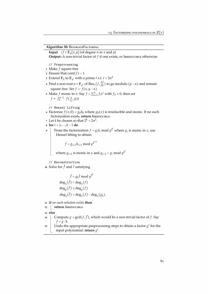
13. Factorizing polynomials in Z[x]
Algorithm 30: BivariateFactoringInput : f ∈ Fq[x, y] (of degree n in x and y)Output :A non-trivial factor of f if one exists, or Irreducible otherwise
// Preprocessing
1 Make f square free2 Ensure that cont( f ) = 13 Extend Fq to Fqt with a prime t s.t. t > 2n2
4 Find a non-root α ∈ Fqt of Resx( f , ∂ f∂x ) to go modulo (y − α) and remain
square free. Set f ← f (x, y − α)
5 Make f monic in x: Say f = ∑ni=1 fixi with fn ≠ 0, then set
f ← f n−1n ⋅ f ( x
fn, y))
// Hensel Lifting
6 Factorize f (x, 0) = g0h0 where g0(x) is irreducible and monic. If no suchfactorization exists, return Irreducible.
7 Let k be chosen so that 2k > 2n2.8 for i = 1,⋯, k − 1 do9 From the factorization f = gihi mod y2i
where gi is monic in x, useHensel lifting to obtain
f = gi+1hi+1 mod y2i+1
where gi+1 is monic in x and gi+1 = gi mod y2i
// Reconstruction
10 Solve for f and ˜ satisfying
f = gk ˜ mod y2k
degx( f ) < degx( f )
degy( f ) ≤ degy( f )
degx(˜) < degx( f )−degx(gk).
11 if no such solution exists then12 return Irreducible.13 else14 Compute g = gcd( f , f ), which would be a non-trivial factor of f . Say
f = g ⋅ h.15 Undo the appropriate preprocessing steps to obtain a factor g′ for the
input polynomial. return g′.
81
13. Factorizing polynomials in Z[x]
13 Factorizing polynomials in Z[x]Lecture 18:March 31st, 2017 We shall now deal with factorizing univariate polynomials over integer coeffi-
cients. This would bear a lot of similarity with factorizing bivariate polynomialsover finite fields. This connection might seem mysterious but turns out there isa good reason for it via a chain of prime ideal containments. Basically, we have
(0) ⊂ (p) ⊂ (p, x) ⊂ Z[x],
(0) ⊂ (y) ⊂ (y, x) ⊂ Fq[x, y],
as the largest chain of prime ideal containments. Even in the algorithm we shalldescribe, we shall be choosing a prime p to play the role that y had in our bivari-ate factorization.
The input is a polynomial f (x) ∈ Z[x]. Unlike earlier, the coefficients arenow integers which can potentially be unbounded so the input size will involvethe size of the coefficients also. Let us assume that each of the coefficient of fhave absolute value at most 2c (i.e., they are c-bit integers). The goal would beto design an algorithm to compute a non-trivial factor (if any exists) in timepoly(n, c).
Size of factors of f (x)
But before we do this, suppose g(x) ∈ Z[x] is a factor of f , why should it evenbe the case that the coefficients of g are small? Is it even reasonable to ask forfactorization? Fortunately, we do have a good bound.
Lemma 13.1 (Mignotte’s Bound). Let f ∈ Z[x] and say each of its coefficients isbounded by 2c in absolute value. If g ∈ Z[x] is a factor of f , then each coefficient of gis bounded by 2n ⋅ nn ⋅ 2cn in absolute value. That is, the coefficients of g are at mostO(n log n + cn) bits long.
Proof. Suppose α ∈ C is a complex root* of f , i.e. f (α) = 0, how large can ∣α∣ be? * - “Wait, why arewe going to complexnumbers now?” Pa-tience.”
If f = a0 + a1x +⋯anxn, then we must have
∣an∣∣αn∣ =
RRRRRRRRRRR
n−1∑i=0
αn−1ai
RRRRRRRRRRR
Ô⇒ ∣αn∣ ≤
RRRRRRRRRRR
n−1∑i=0
αn−1ai
RRRRRRRRRRR
≤ ∣α∣n−1 ⎛
⎝
n−1∑i=0
∣ai∣⎞
⎠
This forces ∣α∣ ≤ n ⋅ 2c.What was the connection with g? Note that the roots of g is just a subset of
the roots of f , and every coefficient of g is a symmetric polynomial in these rootsand they happen to be integers! Now how large can any symmetric polynomialover these roots be? For a very crude bound, each symmetric polynomial is asum of at most 2n terms, each being a product of at most n of the roots of f .Hence, every coefficient of g is at most 2n ⋅ (n ⋅ 2n)n.
82
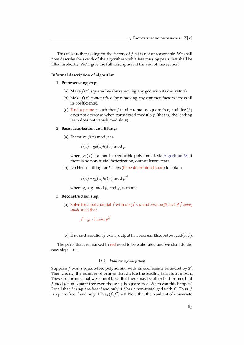
13. Factorizing polynomials in Z[x]
This tells us that asking for the factors of f (x) is not unreasonable. We shallnow describe the sketch of the algorithm with a few missing parts that shall befilled in shortly. We’ll give the full description at the end of this section.
Informal description of algorithm
1. Preprocessing step:
(a) Make f (x) square-free (by removing any gcd with its derivative).(b) Make f (x) content-free (by removing any common factors across all
its coefficients).(c) Find a prime p such that f mod p remains square free, and deg( f )
does not decrease when considered modulo p (that is, the leadingterm does not vanish modulo p).
2. Base factorization and lifting:
(a) Factorize f (x) mod p as
f (x) = g0(x)h0(x) mod p
where g0(x) is a monic, irreducible polynomial, via Algorithm 28. Ifthere is no non-trivial factorization, output Irreducible.
(b) Do Hensel lifting for k steps (to be determined soon) to obtain
f (x) = gk(x)hk(x) mod p2k
where gk = g0 mod p, and gk is monic.
3. Reconstruction step:
(a) Solve for a polynomial f with deg f < n and each coefficient of f beingsmall such that
f = gk ⋅ ˜ mod p2k
(b) If no such solution f exists, output Irreducible. Else, output gcd( f , f ).
The parts that are marked in red need to be elaborated and we shall do theeasy steps first.
13.1 Finding a good prime
Suppose f was a square-free polynomial with its coefficients bounded by 2c.Then clearly, the number of primes that divide the leading term is at most c.These are primes that we cannot take. But there may be other bad primes thatf mod p non-square-free even though f is square-free. When can this happen?Recall that f is square-free if and only if f has a non-trivial gcd with f ′. Thus, fis square-free if and only if Resx( f , f ′) ≠ 0. Note that the resultant of univariate
83

13. Factorizing polynomials in Z[x]
polynomials over integers is also an integer (just a determinant of an integermatrix). Hence, if we choose a prime that does not divide this resultant, wewould be done.
Lemma 13.2. Let f and g be integer polynomials of degree at most n that have coefficientsbounded by 2c. Then, ∣Resx( f , g)∣ ≤ (2n)! ⋅ 22cn.
Proof. The resultant of f and g is the determinant of a matrix of size at most2n× 2n made up of entries bounded by 2c. Hence, its determinant can be at most(2n)! ⋅ 22cn.
Corollary 13.3. There is a prime within the first (cn)2 integers that neither dividesResx( f , f ′) nor the leading coefficient of f .
Proof. The number of primes that divide either the resultant or the leadingcoefficient of f is at most O(cn+n log n). The first (cn)2 integers has more primesthan this.
Thus, we can just run through the first (cn)2 primes and choose a prime pthat works and proceed to the next steps.
13.2 How large should k be?
In the bivariate case, Resx( f , f ) was a polynomial in y, and we chose our k so that2k was bigger than the degree. Here, we just need to work with the magnitudeinstead as the resultants here are just numbers.
But in order to get a bound on the size of Resx( f , f ), we need a bound onthe coeffcients of f . This is promised by the reconstruction step, though we donot know what precisely “small” means there.
Lemma 13.4. Suppose we have an f for whch there is some ˜ ∈ Z[x] such that f tof = gk ˜ mod p2k
with deg f < n and each coefficient of f has absolute value at most 2r.If p2k
> (2n)! ⋅ 22n(r+c), then gcd( f , f ) ≠ 1.
Proof. Consided Resx( f , f ). By Lemma 12.6, there must be polynomials a(x), b(x)such that
Resx( f , f ) = a f + b f
Ô⇒ Resx( f , f ) = a f + b f mod p2k
= agkhk + bgk ˜ mod p2k
= gk(ahk + b ˜) mod p2k.
But the LHS is a number modulo p2kbut the RHS is a multiple by gk, which has
non-zero degree in x. Hence, this forces
Resx( f , f ) = 0 mod p2k.
84
13. Factorizing polynomials in Z[x]
But notice that we chose k so that p2kis bigger than the larest possible value
of Resx( f , f ). Hence, Resx( f , f ) is zero even without the mod. Hence, f and fmust share a common factor.
And as seen earlier Claim 12.7, we know that a solution does indeed exist asg0 must divide some honest-to-God factor of f , and that is a valid choice for f .
What is left therefore is to see how to find a short vector f that is divisible bygk. This is where lattices come in.
13.3 Lattices
Motivation
The reconstruction step required that we look for a polynomial f of degree atmost n− 1 and “small coefficients” such that gk divides it mod p2k
. Since we havesome weird condition on the coefficients, let us try and rewrite it somehow. Saydeg gk = m. As we run over possibilities for ˜ = a0 + a1x +⋯+ an−1−mxn−1−m, thepolynomial gk ˜ is
n−m−1∑i=0
aixigk(x).
What we want is, after we reduce each coefficient modulo p2k, each coefficient is
small. We can express this as
n−m−1∑i=0
aixigk(x)−
n∑i=0
bi p2k
xi,
where we are basically removing any multiple of p2kin each “coordinate” if
possible. We can restate our goal in the following form:
Find an integer linear combination of the vectors
gk(x), xgk(x), . . . , xn−m−1gk(x), p2k, p2k
x,⋯, p2kxn−1
(where each polynomial is thought of as a vector of length n with itscoefficients listed out) of “small length”.
This is what a lattice. Formally, a lattice over Z is defined as follows.Definition 13.5 (Lattice). Let b1, . . . , bm ∈ Zn. The lattice generated by them,denoted by ⟨b1, . . . , bm⟩Z is the set of all integer linear combinations of these vectors.That is,
⟨b1, . . . , bm⟩Z = ∑i
αibi ∶ αi ∈ Z for all i . ◊
Remark 13.6. The subspace spanned by the generating set consists of Q-linear combi-nations of these vectors whereas the lattice is only with integer combinations. In fact,
85

13. Factorizing polynomials in Z[x]
turns out that there is always a generating set of a lattice whose size is equal to the rankof the subspace spanned by them (you’ll see why in Problem Set 2). Furthermore, such agenerating set can be found efficiently.
So we shall assume from now on that whenever we are given a generating setb1, . . . , bm ⊂ Zn, we will assume that m = rank (spanQ b1, . . . , bm). ◊
The Shortest Vector Problem (SVP): Given input vectors b1, . . . , bn that gen-erate a lattice L ⊆ Zn, find a vector bopt ∈ L such that ∥bopt∥ = min0≠b∈L ∥b∥.
Turns out, finding the shortest vector in a given lattice is NP-hard. So itis infeasible to solve the SVP problem in order to use it for our factorizationalgorithm. However, we do not really need the shortest possible solution. Allwe need is a short enough solution. A beautiful algorithm of Lenstra, Lenstra andLovasz give an approximation algorithm for the SVP problem.
Theorem 13.7 (Lenstra, Lenstra, Lovasz). Given integer vectors b1, . . . , bn ⊆ Zn,there is a deterministic polynomial time (in n and the size of coordinates of bis) algorithmthat computes a vector 0 ≠ b ∈ L ∶= ⟨b1, . . . , bn⟩Z such that
∥b∥ ≤ 2(n−1)/2 ⋅ min0≠b′∈L
∥b′∥ .
That is, it gives a 2(n−1)/2-factor approximation to the shortest vector problem.
Before we can describe the algorithm, we would need a few preliminaries,namely the Gram-Schmidt orthogonalization.
13.4 Gram-Schmidt Orthogonalization
The idea of the Gram-Schmidt process is, given a basis B = b1, . . . , bm ⊆ Qn, theGram-Schmidt process output a different basis B∗ = b∗1 , . . . , b∗m that generatethe same space but are pairwise orthogonal. The algorithm is pretty standardand is described below.
86

13. Factorizing polynomials in Z[x]
Algorithm 31: Gram-SchmidtInput :A full rank basis B = b1, . . . , bm ⊆ Qn
Output :An orthogonal basis for the space generated by B
1 for i = 1, . . . , m do2 Compute
b∗i = bi −i−1∑j=1
µi,jb∗j , where µi,j =
⟨bi, b∗j ⟩
⟨b∗j , b∗j ⟩.
3 Define the matrix
M =
⎡⎢⎢⎢⎢⎢⎢⎢⎣
1µ2,1 1⋮ ⋱ ⋱
µm,1 ⋯ µm,m−1 1
⎤⎥⎥⎥⎥⎥⎥⎥⎦
.
return B∗ = b∗1 , . . . , b∗m and M.
It is clear from the description of the algorithm that if we were to list theinput basis vectors as rows of a matrix B, and if B∗ is thought of as the outputvectors listed as rows, then
M ⋅ B∗ = B.
Here are a few simple but important observations.
Observation 13.8. For all i ≤ m, the space generated by b1, . . . , bi is the same asthe space generated by b∗1 , . . . , b∗i .
Observation 13.9. If Si = spanb1, . . . , bi, and if S⊥i is its orthogonal complement,then b∗i+1 is just the projection of bi+1 on to S⊥i .
Observation 13.10. The output of Algorithm 31 would vary if the input vectors arerearranged.
The idea of the LLL algorithm would be the following. We would like to justdo the Gram-Schmidt orthogonalization and output the smallest basis vector,however some of the µi,js may not be integers so these transformations do notstay within the lattice. However, what we shall do is as much as we can ofthe Gram-Schmidt process within the lattice by which we end up with a newbasis that is sort-of-orthogonal. And then will come the magical Lovasz step ofchecking if a particular condition holds and swapping vectors and restarting thewhole process. The algorithm is completely described below, but we’ll prove thecorrectness etc. in the next class.
87

13. Factorizing polynomials in Z[x]
Algorithm 32: LLL AlgorithmInput :A full rank basis B = b1, . . . , bm ⊆ Zn
Output :A (short enough) vector b ∈ ⟨b1, . . . , bm⟩Z
1 repeat2 Using Algorithm 31, compute M, B∗ such that MB∗ = B.
// Do integer row operations on both sides.
3 for i = m,⋯, 1 do4 for j = i − 1,⋯, 1 do5 bi ← bi − ⌈µi,j⌋bj, where ⌈µi,j⌋ is the integer nearest to µi,j.6 Update row i of M accordingly.
// We again have MB∗ = B with now M being lower
triangular and all off-diagonal entries having absolute
value at most 12.
7 if for some 1 ≤ i ≤ m − 1 we have ( 34) ∥b∗i ∥
2> ∥b∗i+1 + µi+1,ib∗i ∥
2 then8 Swap bi and bi+1.9 else
10 return b1
11 until until you return something
This seems to be a mysterious algorithm, not just for the unbounded repeatloop but a rather curious criterion under which we swap some two vectors andrepeat the process. It might seem a bit weird at first, and we will look at it indetail shortly but at the moment, the following exercise should throw some lighton the weird condition.
Exercise 1. On input b1, . . . , bm, suppose Gram-Schmidt outputs b∗1 , . . . , b∗m.Now consider applying the Gram-Schmidt process after swapping the vectors bi andbi+1 and suppose the output vectors are b1, . . . , bm. Then, the following holds:
• For all j < i, we have bj = b∗j .
• For all j > i + 1, we have bj = b∗j .
• bi = b∗i+1 + µi+1,ib∗i .
Therefore, line 7 of Algorithm 32 is asking — Does swapping two successivevectors lead to a significant drop in the length of the i-th Gram-Schmidt vec-tor? If there is such a significant drop (by a factor of 3/4), then we do such a swap.
To show that the above algorithm works, we need to show two things — (1)If it does terminate, whatever it outputs is a good approximation of the shortestvector in the lattice, and (2) the algorithm does terminate in polynomially manysteps.
88

13. Factorizing polynomials in Z[x]
If the algorithm terminates, it is rightLecture 19:April 10th, 2017 Lemma 13.11. Suppose b∗1 , . . . , b∗m is an orthogonal system of vectors (as obtained
by Algorithm 31) on input b1, . . . , bm such that
M ⋅ B∗ = B,
where B and B∗ are matrices whose rows are b1, . . . , bm and b∗1 , . . . , b∗m respec-tively, and M is a lower-triangular matrix with 1s on the diagonal. If bopt is the shortestvector in L, the lattice generated by b1, . . . , bm, then ∥bopt∥ ≥ min
i∥b∗i ∥.
Proof. Say bopt = ∑i αibi such that αi ∈ Z, and let k be the largest index such thatαi ≠ 0. Now, if we express bi = b∗i + ∑
j<iµi,jb∗j , we obtain:
bopt = αkb∗k + (terms involving b∗i for i < k).
Using Pythagoras on the previous equation gives
∥bopt∥2≥ ∣αk∣
2⋅ ∥b∗k ∥
2≥ ∥b∗k ∥
2
as αk is a non-zero integer and therefore ∣αk∣ ≥ 1.
At any time in Algorithm 32 before the swap-step, we do have an equationof the form MB∗ = B and hence we may claim that ∥bopt∥ ≥ mini ∥b∗i ∥. However,the issue is that we must output a vector in the lattice L, and from the rowsof B∗, only b∗1 is guaranteed to lie in L. This is exactly where the terminationcondition helps us.
Whenever Algorithm 32 terminates, the termination condition ensures thefollowing: For all i ∈ 1, . . . , m − 1,
34∥b∗i ∥
2≤ ∥b∗i+1 + µi+1,ib
∗i ∥
2
= ∥b∗i+1∥2+ µ2
i+1,i ∥b∗i ∥2 (Pythagoras)
≤ ∥b∗i+1∥2+
14∥b∗i ∥
2(∣µi+1,i∣ ≤
12)
Ô⇒ ∥b∗i+1∥2≥
∥b∗i ∥2
2
An orthogonal basis that satisfies ∥b∗i+1∥2≥ ∥b∗i ∥
2/2 is called a reduced Basis.
Combining the above with Lemma 13.11 makes the following plain.
Proposition 13.12. If b∗1 , . . . , b∗m is a reduced basis then ∥b1∥2≤ 2n−1 ∥b∗opt∥
2.
The algorithm terminates in polynomially many steps
So, what have we established till now? We know that if Algorithm 32 does termi-nate then, by Proposition 13.12, ∥b1∥ = ∥b∗1∥ ≤ 2
n−12 ∥bopt∥. Thus, we may safely
89

13. Factorizing polynomials in Z[x]
output b1, to achieve an approximation ratio of 2n−1
2 .
Now, let us understand why Algorithm 32 does terminate in a polynomialnumber of steps (in n, m and the size of the coordinates of bi’s). A priori, it is notclear that the algorithm stops at all. To this end suppose at line 7 we find thatfor some 1 ≤ i ≤ m − 1 we have 3
4 ∥b∗i ∥2> ∥b∗i+1 + µi+1,ib∗i ∥
2, then we swap bi andbi+1. Now, b1, . . . , bi+1, bi, . . . , bm becomes the input to Algorithm 31 at line2. Suppose the output vectors of the Gram-Schmidt process are b1, . . . , bm,represented as rows in the matrix B. Observe that the subsequent run throughlines 3–6 does not perturb B. Therefore, by Exercise 1 we obtain that b1, . . . , bm
and b∗1 , . . . , b∗m differ only on the (i)th and (i + 1)th vector, and further bi =
b∗i+1 + µi+1,ib∗i . This means that 34 ∥b∗i ∥
2> ∥bi∥
2.Hmmm . . . so the norms of all the vectors except the (i)th and (i + 1)th stay
the same and the norm of the (i)th one drops by a constant factor. If only, we hada handle on the norm of the (i + 1)th vector, we could argue that some potential
function, likem∏i=1
∥b∗i ∥2 is decreasing each time the swap at line 7 is performed,
and hence Algorithm 32 must terminate within so-and-so number of steps.Great! Unfortunately*,∏m
i=1 ∥b∗i ∥2 stays constant throughout Algorithm 32! * or fortunately!
To see this, observe the elementary row operations performed on the inputmatrix B: as we noted earlier, each operation is either a swap (line 7) or of theform Ri → Ri −∑j β jRj, where β j ∈ Z. These are all invertible operations on thelattice. Consider B′ = RB where B′ is any intermediate form that B acquires andR is the corresponding m ×m matrix representing the accrued Row-elementaryoperations. R is an integer matrix and invertible; further R−1 is also and integermatrix!* Since, det (R) and det (R−1) are both integers and det (R)×det (R−1) = * Why? Think about
reversing all theRow-elementary op-erations performed.
1, we obtain det (R) = ±1. Such matrices (R such that det R = ±1) are infact calledunimodular matrices and these are precisely transformations we can perform onthe lattice basis without changing the lattice.
Observation 13.13. If the rows of an m × n integer matrix B is a basis of some latticeand B′ is another m × n integer matrix. Then, rows of B and the rows of B′ generate thesame lattice if and only if B′ = RB where R is an m ×m unimodular integer matrix.
Therefore, we’d like to say that ∣det B∣ = ∣det B′∣ throughout, but wait, thesematrices aren’t even square matrices. But let us make them square matrices bylooking at BBT and B′B′T instead. Hence, det BBT = det B′B′T as B′ = RB anddet R = ±1.
Let us couple this observation with the fact that MB∗ = B, and M is lowertriangular with all the diagonal entries 1 implying that det (M) = 1. Thus, bythe orthogonality of the rows of B∗, we establish that
det(B∗B∗T) =
m∏i=1
∥b∗i ∥2= det (BBT)
stays invariant.
90
13. Factorizing polynomials in Z[x]
All this effectively tells us that using ∏mi=1 ∥b∗i ∥
2 as a potential function isuseless because this never changes throughout the algorithm. Now, it is time formore magic. Instead of looking at the potential function∏m
i=1 ∥b∗i ∥2, we look at
the following variant:
Di ∶=i∏j=1
∥b∗j ∥2
Φ ∶=m∏i=1
Di
∶= ∥b∗1 ∥2m
∥b∗2 ∥2m−2
⋯ ∥b∗m∥2
Lemma 13.14. If B is an integer matrix, then each Di is also an integer and is non-zero.
Proof. Consider the Gram-Schmidt equation MB∗ = B where B is an upper-triangular, if we focus on just the first i rows of B and B∗, then we can restrictourselves to the i × i principal minor of M to get an equation MiB∗i = Bi. SinceM was upper-triangular with 1s on the diagonal, Mi continues to share thatproperty. Therefore,
det BiBTi = det B∗i (B∗i )
T
= ∥b∗1 ∥2⋯ ∥b∗m∥
2
=∶ Di
And since we are starting with a full-rank basis, none of the b∗i s are zero andhence Di is non-zero.
Lemma 13.15. Every swap at line 7 of Algorithm 32 reduces Φ by at least 34
.
Proof. Suppose, in some iteration, at line 7 we swap bi and bi+1, and after arun through lines 2–6, we obtain b1, . . . , bm. Let D′
i =∏ij=1 ∥bj∥
2 Then, by ourearlier observations and Exercise 1 it is clear that for j < i, we have Dj = D′
j .
Additionally, D′i ≤
34
Di.We also have Di+1 = D′
i+1. This is because swapping rows i and i + 1 does notchange det(Bi+1BT
i+1) = Di+1. Similarly, for j > i + 1, Dj = D′j .
Hence, only Di reduces by a factor of 3/4, and all other Djs stay the same.Therefore,∏j D′
j ≤ ( 34)∏j Dj.
Now we know that every swap step reduces our potential function by atleast a factor of 3/4. We also know from Lemma 13.14 that Φ is always a positiveinteger. This should let us upper-bound the number of swaps throughout if wehave a bound on how large Φ is in the beginning of the algorithm.
Proposition 13.16. Φ is maximum at the beginning of Algorithm 32, where ∣Φ∣ ≤
(m! × (n22c)m)m, where c is the maximum length of the bit representations of thecoefficients of the input vectors b1, . . . , bm.
91
13. Factorizing polynomials in Z[x]
Proof. As seen in Lemma 13.14, Di = det BiBTi . If each of the entries of B are
integers of magnitude at most 2c, each entry of the m × m matrix BiBTi has
magnitude at most n22c. Therefore, Di = det(BiBTi ) is at most m!(n22c)m.
Proposition 13.17. Algorithm 32 performs at most O (m2c +m2 log (m)+m log (n))swap operations at line 7, and hence runs in time polynomial in n, m and the size of thecoordinates of bi’s.
And that completes the analysis of the LLL algorithm and hence Theo-rem 13.7, and hence concludes the algorithm to factorize polynomials in Z[x].
Algorithm 33: Factorization over integersInput : f ∈ Z[x] of degree n, and coefficients bounded by 2c
Output :A non-trivial factor of f if one exists, or Irreducible otherwise
// Preprocessing
1 Make f square free2 Ensure that cont( f ) = 13 Find a prime p such that f mod p is square-free and deg( f ) and p does not divide
the leading coefficient of f .
// Hensel Lifting
4 Factorize f (x) = g0h0 mod p where g0(x) is irreducible and monic. If no suchfactorization exists, return Irreducible.
5 Let k be chosen so that p2k> 23cn3
.6 for i = 1,⋯, k − 1 do7 From the factorization f = gihi mod p2i
where gi is monic, use Hensel lifting toobtain
f = gi+1hi+1 mod p2i+1
where gi+1 and gi+1 = gi mod p2i
// Reconstruction
8 If deg gk = m, construct the lattice
L ∶= ⟨gk(x), xgk(x), . . . , xn−m−1gk(x), p2k, p2k
x, . . . , p2kxn−1⟩
Z.
Using Algorithm 32, compute a short vector f (x) ∈ L.
9 if ∥ f ∥ > 23cn2then
// If f was reducible, then LLL ought to find an f with
coefficients at most 22cn2+O(n).
10 return Irreducible.11 else12 Compute g = gcd( f , f ), which would be a non-trivial factor of f . Say f = g ⋅ h.13 Undo the appropriate preprocessing steps to obtain a factor g′ for the input
polynomial. return g′.
92
14. Kaltofen’s black-box factorization algorithm
14 Kaltofen’s black-box factorization algorithmLecture 20:April 10th, 2017 The algorithms we have seen in section 12 that we can use an algorithm for k-
variate factorization and boot-strap it with the Hensel Lifting approach to obtaina factorization algorithm for (k + 1)-variate polynomials. This works of course,but the running time degrades very badly in k. Hence, using this approach forfactorizing multivariate polynomials (where the number of variables n grows)is infeasible.
The other question is, if we are dealing with polynomials over many variables,we could potentially have many monomials for such a polynomial. How is theinput provided to us?
Kaltofen came up with a remarkable algorithm where given just blackboxaccess to the polynomial (that is, all we know are its degree, number of variables,and we are only allowed to evaluate the polynomial at any chosen point of ours),we can construct blackboxes for each of its factors as well! Firstly, it is not at allclear that the factors should even be efficiently computable in the first place!Kaltofen’s result shows that they indeed can be, and also construct a randomizedalgorithm to find blackboxes for the factors given a blackbox for the polynomial.
A key ingredient in the algorithm is the Hilbert’s Irreducibility theoremTheorem 14.1 which gives a test for irreducibility of multivariate polynomials.
Hilbert’s irreducibility theorem
If we wish to come up with a blackbox factorization algorithm, at the very leastwe should be able to check if a given polynomial is irreducible or not. We knowhow to test for irreducibility for univariate polynomials using any of the factoringalgorithms we have seen previously. A natural approach seems to be to reduce tothis case, by substituting each variable xi with a polynomial function ai(t) andchecking for the irreducibility of the univariate polynomial f (a1(t), . . . , an(t)).However there is an obvious reason why this idea won’t work because if thefield is C, every univariate polynomial factorizes into linear factors.
The following remarkable theorem shows that a random bivariate substitutionpreserves irreducibility:
(x, y1, . . . , yn)↦ (x, a1t + b1, . . . , ant + bn).
For simplicity, we shall state the theorem for polynomials that are monic in x,but as we have seen earlier, this can very easily be ensured by minor massaging.
Theorem 14.1 (Hilbert’s Irreducibility Theorem). Let f (x, y1, . . . , yn) be a degreed polynomial which is monic in x. Suppose S ⊆ F and
Pra,b∈Sn
[ f (x, a1t + b1, . . . , ant + bn) is reducible ] ≥O(d5)
∣S∣
then f (x, y1, . . . , yn) is reducible.
We shall prove this shortly but for now let us assume this and completeKaltofen’s algorithm.
93
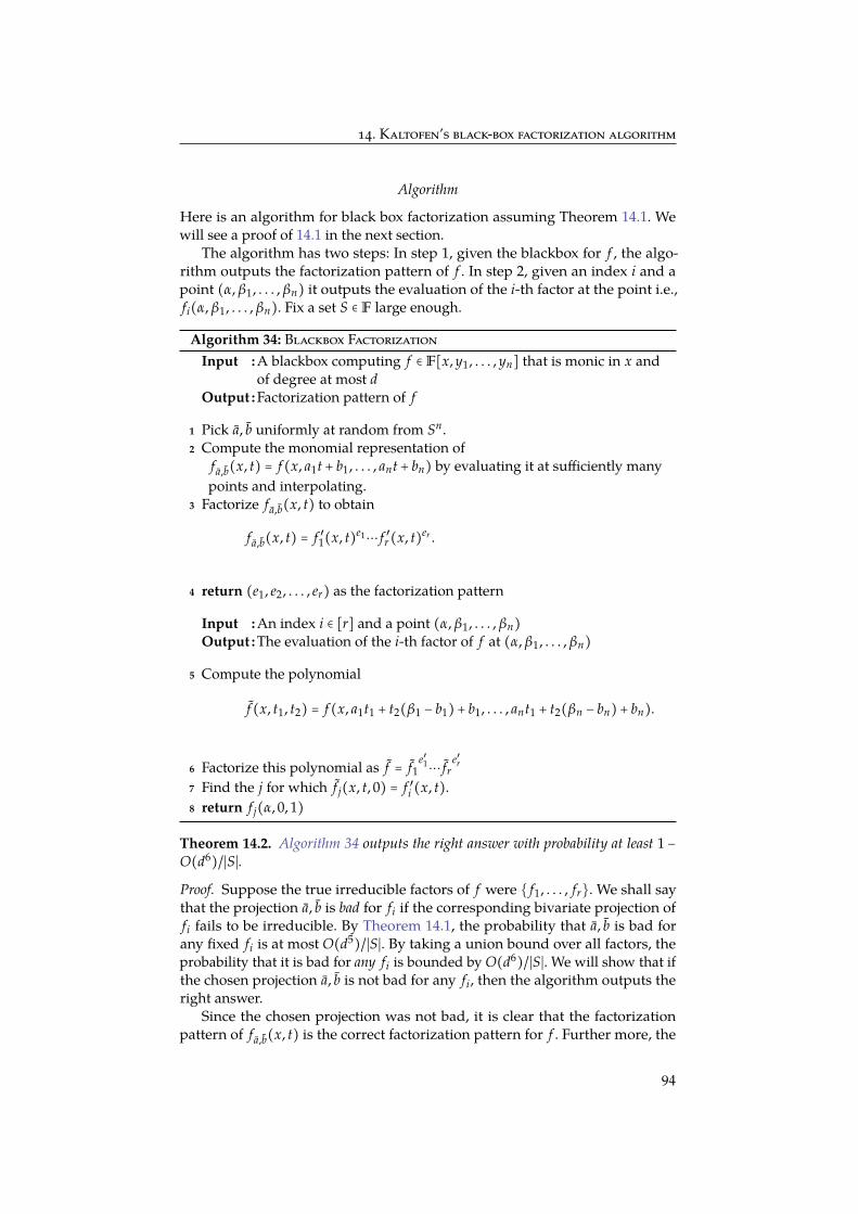
14. Kaltofen’s black-box factorization algorithm
Algorithm
Here is an algorithm for black box factorization assuming Theorem 14.1. Wewill see a proof of 14.1 in the next section.
The algorithm has two steps: In step 1, given the blackbox for f , the algo-rithm outputs the factorization pattern of f . In step 2, given an index i and apoint (α, β1, . . . , βn) it outputs the evaluation of the i-th factor at the point i.e.,fi(α, β1, . . . , βn). Fix a set S ∈ F large enough.
Algorithm 34: Blackbox FactorizationInput :A blackbox computing f ∈ F[x, y1, . . . , yn] that is monic in x and
of degree at most dOutput :Factorization pattern of f
1 Pick a, b uniformly at random from Sn.2 Compute the monomial representation of
f a,b(x, t) = f (x, a1t + b1, . . . , ant + bn) by evaluating it at sufficiently manypoints and interpolating.
3 Factorize f a,b(x, t) to obtain
f a,b(x, t) = f ′1(x, t)e1⋯ f ′r(x, t)er .
4 return (e1, e2, . . . , er) as the factorization pattern
Input :An index i ∈ [r] and a point (α, β1, . . . , βn)
Output :The evaluation of the i-th factor of f at (α, β1, . . . , βn)
5 Compute the polynomial
f (x, t1, t2) = f (x, a1t1 + t2(β1 − b1)+ b1, . . . , ant1 + t2(βn − bn)+ bn).
6 Factorize this polynomial as f = f1e′1⋯ fr
e′r
7 Find the j for which f j(x, t, 0) = f ′i (x, t).8 return f j(α, 0, 1)
Theorem 14.2. Algorithm 34 outputs the right answer with probability at least 1 −O(d6)/∣S∣.
Proof. Suppose the true irreducible factors of f were f1, . . . , fr. We shall saythat the projection a, b is bad for fi if the corresponding bivariate projection offi fails to be irreducible. By Theorem 14.1, the probability that a, b is bad forany fixed fi is at most O(d5)/∣S∣. By taking a union bound over all factors, theprobability that it is bad for any fi is bounded by O(d6)/∣S∣. We will show that ifthe chosen projection a, b is not bad for any fi, then the algorithm outputs theright answer.
Since the chosen projection was not bad, it is clear that the factorizationpattern of f a,b(x, t) is the correct factorization pattern for f . Further more, the
94

14. Kaltofen’s black-box factorization algorithm
polynomial f (x, t1, t2) is constructed so that
f (x, t, 0) = f a,b(x, t) and f (α, 0, 1) = f (α, β1, . . . , βn).
The only issue is that when we factorize f , eventhough every factor of f corre-sponds to a factor of f a,b(x, t), the order might be shuffled. But since they are allirreducible and distinct, the correct order can be found by checking for the rightj so that f j(x, t, 0) = f ′i (x, t).
The probability can also be amplified by trying out many projections a, band choosing one that yields the coarsest factorization of f a,b(x, t).
14.1 Proof of Hilbert’s Irreducibility theorem
We would need the following standard fact that a non-zero polynomial cannotbe zero too often. This is called the
Schwartz Lemma orthe Schwartz-ZippelLemma or theSchwartz-Zippel-DeMillo-LiptonLemma or Øre’sLemma.
Lemma 14.3 (Øre,Schwartz,Zippel,DeMillo-Lipton). If f is a non-zero polynomialof degree at most d and S ⊆ F is a finite set then
Pra∈Sn
[ f (a) = 0] ≤d∣S∣
.
We are given that a random bivariate projection f a,b(x, t) is reducible veryoften and we would like to show that f must be reducible. As a warm-up, we willfirst show that if f0,b(x) is not square-free too often, then f cannot be square-free.
Not square-free too often implies reducible
Lemma 14.4. Suppose f is a polynomial monic in x and say deg( f ) ≤ d. If it is thecase that Pr [ f (x, b1, . . . , bn) not square-free ] ≥ 2d2
∣S∣ then f (x, y1, . . . , yn) is reducible.
Proof. Note that f (x, b1, . . . , bn) ∈ F[x] is a univariate polynomial in x. Considerthe polynomial R((y)) ∶= Resx ( f , ∂ f
∂x) ∈ F[y]. For every b such that f (x, b1, . . . , bn)
is not square-free, we know that R(b)) = 0. This implies that R(y) is a polynomialof degree at most 2d2 but is zero with probability more than 2d2/∣S∣ on Sn andhence by Lemma 14.3 we must have that R(y) = 0.
This then implies that f and ∂ f∂x have a non-trivial gcd in F(y)[x], which
by Gauss’s Lemma (Theorem 12.2) means that they have a non-trivial gcd inF[x, y]. This of course implies that f (x, y) not just reducible, but in fact notsquare-free.
Therefore, we may assume that there are many points in b ∈ Sn wheref (x, b1, . . . , bn) is square-free (for otherwise, Lemma 14.4 already shows thatf is reducible). Without loss of generality, let us assume that f (x, 0, . . . , 0) issquare-free. This essentially allows us to forget the b and instead work withf (x, a1t, . . . , ant). The problem therefore has reduced to the following — we are
95

14. Kaltofen’s black-box factorization algorithm
given a monic (in x) polynomial f (x, y1, . . . , yn) of degree at most d such thatf (x, 0, . . . , 0) is square-free and also
Pra∈Sn
[ f (x, a1t, . . . , ant) is reducible] > O(d5)
∣S∣,
and we want to conclude that f must be reducible.
The main sub-case: f (x, 0, . . . , 0) is square-free
Define the following auxiliary polynomials which will be useful in arguing thereducibility of f
p(x, t, y1, . . . , yn) ∶= f (x, a1t, . . . , ant).
For every a ∈ Fn define a bivariate polynomial
f a(x, t) ∶= f (x, at, . . . , ant).
Notice that p(x, t, a1, . . . , an) = f a(x, t) and p(x, 1, y1, . . . , yn) = f (x, y1, . . . , yn).The following lemma says that it suffices to show that p(x, t, y) is reducible.
Claim 14.5. If p(x, t, y) is reducible, then f (x, y) is reducible.
Proof. If p is reducible, then p can be written as
p(x, t, y) = A(x, t, y) ⋅ B(x, t, y)
Recall that f (x, y) = p(x, 1, y). Therefore f (x, y) = A(x, 1, y) ⋅ B(x, 1, y). The onlything to be checked is if A(x, 1, y) or B(x, 1, y) becomes a constant. But thiscannot happen as p is also monic in x and hence so are A and B. ThereforeA(x, 1, y), B(x, 1, y) are non-constants and f is reducible.
Hensel lifting a bivariate factorization
Just like in section 12, we would be using Hensel lifting heavily. The first step isto get better factorizations for f a(x, t). We start with
f a(x, t) = g0(x) ⋅ h0(x) mod t
where g0(x) is monic in x and is coprime with h0(x). This can be done as we knowf a(x, t) mod t = f (x, 0, . . . , 0) which is square-free. Starting from this solution,we apply Hensel lifting repeatedly to get
f a(x, t) = g0(x) ⋅ h0(x) mod t
⋮
f a(x, t) = gk,a(x, t) ⋅ hk,a(x, t) mod tk,
where gk,a(x, t) is monic in x, and again we shall lift until k > 2d2.
96

14. Kaltofen’s black-box factorization algorithm
At the face of it, if we were to start with a different choice of a, the polyno-mial gk,a(x, t) could be completely different. The following lemma says that thedifferent gk,a(x, t)s are globally correlated.
Lemma 14.6. There is a polynomial gk(x, t, y) such that for every a we have gk,a(x, t) =gk(x, t, a)).
Proof. Consider obtaining factorizations of f (x, y1,⋯, yn) via Hensel Lifting, bystarting with
f (x, y1, . . . , yn) = g0(x) ⋅ h0(x) mod ⟨y1,⋯, yn⟩.
We have the same start as f (x, y1, . . . , yn) mod ⟨y1,⋯, yn⟩ = f (x, 0, . . . , 0). ApplyHensel lifting here gives
f (x, y1, . . . , yn) = g′k(x, y) ⋅ h′k(x, y) mod ⟨y1,⋯, yn⟩k.
Bear with the ′ on the RHS; that’s only because these are not quite the gk we areafter. What the above equation means is that if we consider the polynomial
f (x, y1, . . . , yn)− g′k ⋅ h′k,
then every monomial in this polynomial has y-degree at least k. Therefore, if wescale the y-variables by t
f (x, ty1, . . . , tyn)− g′k(x, ty1, . . . , tyn) ⋅ h′k(x, ty1, . . . , tyn)
now is divisible by tk. In other words,
f (x, ty1, . . . , tyn) = g′k(x, ty1, . . . , tyn) ⋅ h′k(x, ty1, . . . , tyn) mod tk
Ô⇒ f a(x, t) = g′k(x, ta1, . . . , tan) ⋅ h′k(x, ta1, . . . , tan) mod tk
∶= gk(x, t, a)hk(x, t, a) mod tk
where gk(x, t, y) ∶= g′k(x, ty1,⋯, tyn). Observe that gk(x, t, a) is also monic in x,and is equal to g0(x) mod t and we also have a lifted equation
f a(x, t) = gk,a(x, t) ⋅ hk,a(x, t) mod tk.
By the uniqueness of Hensel Lifting (Theorem 12.1) we have that gk,a(x, t) =
gk(x, t, a) for all a.
Reconstructing a factor of p(x, t, y)
Like in Algorithm 30, the last step would be to reconstruct a factor of p(x, t, y)from a sufficiently lifted factor gk(x, t, y). As in the bivariate case, we wouldlike to build a system of equations that should have a solution if p(x, t, y) isreducible.
We shall interpret gk(x, t, y) as a bivariate polynomial, by thinking of it as anelement of F(y)[x, t]. The system of equations solves for a possible f (x, t), ˜(x, t) ∈
97
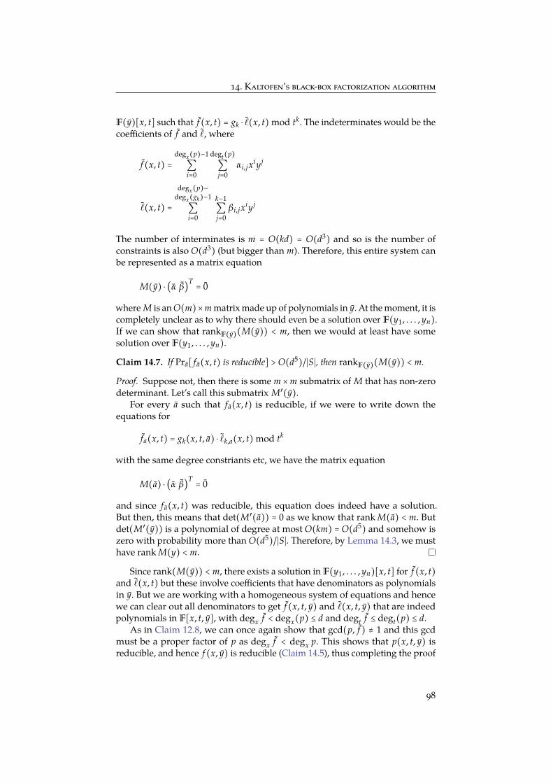
14. Kaltofen’s black-box factorization algorithm
F(y)[x, t] such that f (x, t) = gk ⋅ ˜(x, t) mod tk. The indeterminates would be thecoefficients of f and ˜, where
f (x, t) =degx(p)−1
∑i=0
degt(p)
∑j=0
αi,jxiyj
˜(x, t) =
degx(p)−degx(gk)−1
∑i=0
k−1∑j=0
βi,jxiyj
The number of interminates is m = O(kd) = O(d3) and so is the number ofconstraints is also O(d3) (but bigger than m). Therefore, this entire system canbe represented as a matrix equation
M(y) ⋅ (α β)T= 0
where M is an O(m)×m matrix made up of polynomials in y. At the moment, it iscompletely unclear as to why there should even be a solution over F(y1, . . . , yn).If we can show that rankF(y)(M(y)) < m, then we would at least have somesolution over F(y1, . . . , yn).
Claim 14.7. If Pra[ f a(x, t) is reducible] > O(d5)/∣S∣, then rankF(y)(M(y)) < m.
Proof. Suppose not, then there is some m ×m submatrix of M that has non-zerodeterminant. Let’s call this submatrix M′(y).
For every a such that f a(x, t) is reducible, if we were to write down theequations for
fa(x, t) = gk(x, t, a) ⋅ ˜k,a(x, t) mod tk
with the same degree constriants etc, we have the matrix equation
M(a) ⋅ (α β)T= 0
and since f a(x, t) was reducible, this equation does indeed have a solution.But then, this means that det(M′(a)) = 0 as we know that rank M(a) < m. Butdet(M′(y)) is a polynomial of degree at most O(km) = O(d5) and somehow iszero with probability more than O(d5)/∣S∣. Therefore, by Lemma 14.3, we musthave rank M(y) < m.
Since rank(M(y)) < m, there exists a solution in F(y1, . . . , yn)[x, t] for f (x, t)and ˜(x, t) but these involve coefficients that have denominators as polynomialsin y. But we are working with a homogeneous system of equations and hencewe can clear out all denominators to get f (x, t, y) and ˜(x, t, y) that are indeedpolynomials in F[x, t, y], with degx f < degx(p) ≤ d and degt f ≤ degt(p) ≤ d.
As in Claim 12.8, we can once again show that gcd(p, f ) ≠ 1 and this gcdmust be a proper factor of p as degx f < degx p. This shows that p(x, t, y) isreducible, and hence f (x, y) is reducible (Claim 14.5), thus completing the proof
98
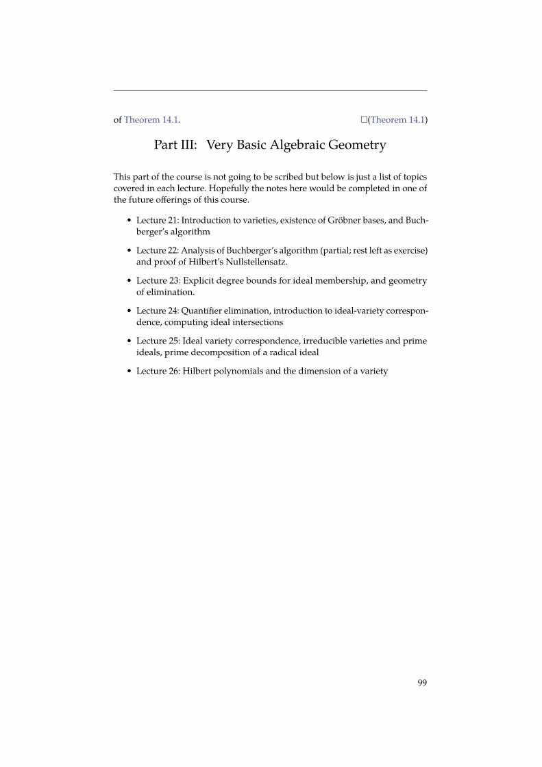
of Theorem 14.1. (Theorem 14.1)
Part III: Very Basic Algebraic Geometry
This part of the course is not going to be scribed but below is just a list of topicscovered in each lecture. Hopefully the notes here would be completed in one ofthe future offerings of this course.
• Lecture 21: Introduction to varieties, existence of Grobner bases, and Buch-berger’s algorithm
• Lecture 22: Analysis of Buchberger’s algorithm (partial; rest left as exercise)and proof of Hilbert’s Nullstellensatz.
• Lecture 23: Explicit degree bounds for ideal membership, and geometryof elimination.
• Lecture 24: Quantifier elimination, introduction to ideal-variety correspon-dence, computing ideal intersections
• Lecture 25: Ideal variety correspondence, irreducible varieties and primeideals, prime decomposition of a radical ideal
• Lecture 26: Hilbert polynomials and the dimension of a variety
99

List of scribes
• Lecture 1, 2: Ramprasad Saptharishi
• Lecture 3: Somnath Chakraborty
• Lecture 4: Anamay Tengse
• Lecture 5: Prerona Chatterjee
• Lecture 6: Suhail Sherif
• Lecture 7: Gunjan Kumar
• Lecture 8: Siddharth Bhandari
• Lecture 9: Prerona Chatterjee
• Lecture 10/11: Tulasi mohan Molli
• Lecture 12: Ramprasad Saptharishi
• Lecture 13: Kshitij Gajjar
• Lecture 14: Somnath Chakraborty
• Lecture 15: Suhail Sherif
• Lecture 16: Prerona Chatterjee
• Lecture 17: Anamay Tengse
• Lecture 18: Ramprasad Saptharishi
• Lecture 19: Siddharth Bhandari
• Lecture 20: Tulasi mohan Molli & Ramprasad Saptharishi
100


![TIFR JGEEBILS Question Paper : 2012ibsacademy.co.in/solved papers/TIFR JGEEBILS Papers/gs_2012.pdf · M.Sc. & Integrated Ph.D. [ JAM-IIT , JNU, TIFR, IISC ] GS-2012 Question paper:](https://static.fdocuments.us/doc/165x107/5ea06110b1ac4e2262464ea4/tifr-jgeebils-question-paper-paperstifr-jgeebils-papersgs2012pdf-msc-.jpg)