Mathematical Engineering

Alexander A. Avdeev

Bubble Systems

Mathematical Engineering

Series editors

Claus Hillermeier, Neubiberg, GermanyJörg Schröder, Essen, GermanyBernhard Weigand, Stuttgart, Germany

More information about this series at http://www.springer.com/series/8445

Alexander A. Avdeev

Bubble Systems

123

Alexander A. AvdeevDmitrovskoe shosse46-1-6127238 MoscowRussiaE-mail: alex3@safe-mail.net

ISSN 2192-4732 ISSN 2192-4740 (electronic)Mathematical EngineeringISBN 978-3-319-29286-1 ISBN 978-3-319-29288-5 (eBook)DOI 10.1007/978-3-319-29288-5

Library of Congress Control Number: 2016933801

© Springer International Publishing Switzerland 2016This work is subject to copyright. All rights are reserved by the Publisher, whether the whole or partof the material is concerned, specifically the rights of translation, reprinting, reuse of illustrations,recitation, broadcasting, reproduction on microfilms or in any other physical way, and transmissionor information storage and retrieval, electronic adaptation, computer software, or by similar or dissimilarmethodology now known or hereafter developed.The use of general descriptive names, registered names, trademarks, service marks, etc. in thispublication does not imply, even in the absence of a specific statement, that such names are exempt fromthe relevant protective laws and regulations and therefore free for general use.The publisher, the authors and the editors are safe to assume that the advice and information in thisbook are believed to be true and accurate at the date of publication. Neither the publisher nor theauthors or the editors give a warranty, express or implied, with respect to the material contained herein orfor any errors or omissions that may have been made.

Printed on acid-free paper

This Springer imprint is published by Springer NatureThe registered company is Springer International Publishing AG Switzerland

Preface

The main purpose of this book is to bring together into a coherent system all ourknowledge about the physical mechanisms governing the laws of behaviour of boththe simplest bubble systems consisting of single bubbles and of involved systems,which occur, for example, in bubble flows or during bubbling.

Due to the rapid progress in science, both textbooks and scarce scientificmonographs, partially embracing this field of knowledge, tend to age rather quickly,often losing their actualité right after publication. I would like very much that thisbook does not share such a fate. This wish has determined its structure.

First, we give a systematic treatment of the fundamental problems describing thedynamics of single bubbles (laws of their growth, collapse, fragmentation andemersion in the gravitational field, pulsation and so on.). The use of modernsoftware products for analytical studies helps to obtain new quite surprising resultseven for these classical problems, whose authors in due time remarkably combineddeep physical sense, serious mathematical technique, and enormous amount ofcomputational and analytical work to obtain rigorous analytical solutions.Moreover, despite the classical nature of the problems under consideration, forsome of them the complete analytical solutions were obtained only in the past twodecades and at present are unknown to the broad research community.

Second, based on these fundamental solutions it is possible to put forward, in alarge number of cases, fairly rigorous analytic solutions of next-level problems,which are traditionally farmed out to experimentalists or specialists in the field ofcomputational fluid dynamics. As example, we may mention the problems onhydrodynamics of bubble flows in channels, sizes of bubbles, true void fraction,hydraulic resistance during boiling of subcooled liquid under forced motion con-ditions, and so on. Despite the fact that in a number of respects we cannot avoidusing the numerical methods, the particular analytic solutions, as well as therecourse to qualitative methods of investigations residing in consistent applicationof similarity methods, enable one to carry out the results of analysis to designrelations, which secure the corresponding passages to the limit and have wide rangeof applications and high accuracy.

v

Third, from the methodological point of view, of great value are the conceptualdevelopments in the field of bubble flows, and in particular, the theory of boilingshock, which was created by the author in the 1980s, and the applications of theReynolds analogy in the study of nonequilibrium two-phase flows.

The systematic use of the theory of boiling shock has enabled one to explain,and in many cases to predict, quite a number of experimental effects accompanyingthe processes of discharge of flashing liquid, the processes of unsteady flashing withrapid pressure relief, and to build on its basis methods for calculation of similarphenomena.

Reynolds analogy for flows with ‘double disequilibrium’ (superheated near-walllayer of liquid—subcooled liquid in the core), which often occur inhigh-performance cooling systems, proved a fairly natural tool in the study ofprocesses of radial transfer of heat and momentum, providing thereby a basis forobtaining fairly rigorous analytic solutions of the heat exchange and hydrodynamicsof such flows.

There are already thousands of scientific and engineering papers relating tononequilibrium two-phase flows. Frequently, these studies consider the samephenomena from quite different (and in a number of cases from directly opposite)viewpoints. In some cases (fortunately, its number is quite narrow), erroneousapproaches migrate from one paper to another to gradually become traditional.

Despite the fact that this branch of science reached its full flowering in the 1970–80s due to the rapid development of nuclear and aerospace engineering, theresearch activity in this field has been quite intensive up to now, which can beexplained by its operational and scientific significance. Consequently, a youngscientist, who has received a good fundamental background and begins his or herstudy in this field, will only after several years be able to orientate in this multi-dimensional space, to be capable of distinguishing the important tendencies of thetheory from the dead-end tracks.

A research engineer embarking on a study of nonequilibrium two-phase systemsshould be familiar with numerous classical disciplines like the thermodynamics andthe theory of the properties of matter, the mechanics of liquid, gas dynamics as wellas the theory of heat and mass transfer. General textbooks and handbooks on thesescientific disciplines contain such a huge amount of information that they cannotalways be comprehended and made valuable by an amateur in thermal physics.A serious problem for a student is the choice of subdisciplines that are vital in his orher studies.

In this process, contacts with elder colleagues and supervisors are invaluable.Maturing of a young scientist is believed to be additionally facilitated by this book,which includes the principal achievements in the construction of the theory andillustrates application of the principal tools for its further development.

In writing this book, the author was mainly focused on the demands of graduateand postgraduate students specializing in two-phase flows physics. This book willbe a useful complement to existing textbooks on heat exchange and gas dynamics,with the aim toward in-depth study of these disciplines and providing help incomprehending the fundamentals of the theory of bubble systems.

vi Preface

The true needs of practicing professionals and postgraduate students are not farapart. Both require, above all, an understanding of the fundamentals of runningprocesses, which is the main purpose of this book.

All solutions, without exception (both analytic and numerical), obtained in thisbook expand to fairly simple design formulas, many of which are put forward forthe first time. Hence, this book also serves as a detailed handbook that can beconveniently used in analytical, numerical and design practice.

In conclusion, the author expresses his sincere gratitude to his numerous col-leagues, coworkers and friends, whose discussions and valuable comments wereinstrumental in bringing the book to its final form.

The author is deeply indebted to Prof. Bernhard Weigand (Stuttgart University),whose courteous attention and support encouraged him in this endeavour.

A great role in the forming of the author’s entire scientific outlook was played indue time by his supervisor Prof. Dmitry Labuntsov (1929–1992). The fact that thereader takes this book in his or her hands means that Labuntsov’s ideas continue todevelop and his blessed memory will live on.

Moscow Alexander A. AvdeevDecember 2015

Preface vii

Contents

1 Introduction. General Principles of Description of Two-PhaseSystems . . . . . . . . . . . . . . . . . . . . . . . . . . . . . . . . . . . . . . . . . . . . 11.1 Two-Phase Systems . . . . . . . . . . . . . . . . . . . . . . . . . . . . . . . 11.2 Methods of Mathematical Description

of Two-Phase Systems . . . . . . . . . . . . . . . . . . . . . . . . . . . . . 31.2.1 Detailed Description . . . . . . . . . . . . . . . . . . . . . . . . . 31.2.2 Unit Cell Models . . . . . . . . . . . . . . . . . . . . . . . . . . . 41.2.3 Single Continuum Models . . . . . . . . . . . . . . . . . . . . . 51.2.4 Models of Multispeed Medium . . . . . . . . . . . . . . . . . 7

1.3 Incorporation of Phases. . . . . . . . . . . . . . . . . . . . . . . . . . . . . 111.3.1 Coordinate Systems . . . . . . . . . . . . . . . . . . . . . . . . . 111.3.2 Coupling Conditions . . . . . . . . . . . . . . . . . . . . . . . . . 13

1.4 Intensity of Phase Transitions . . . . . . . . . . . . . . . . . . . . . . . . 201.4.1 Quasi-Equilibrium Scheme . . . . . . . . . . . . . . . . . . . . 201.4.2 Phase Transitions . . . . . . . . . . . . . . . . . . . . . . . . . . . 22

1.5 The Structure of the Book . . . . . . . . . . . . . . . . . . . . . . . . . . . 27References . . . . . . . . . . . . . . . . . . . . . . . . . . . . . . . . . . . . . . . . . . 33

2 Dynamics of Bubbles in an Infinite Volume of Liquid . . . . . . . . . . 352.1 The Problems of Force Controlled Bubble Evolutions . . . . . . . . 352.2 The Rayleigh-Lamb Equation . . . . . . . . . . . . . . . . . . . . . . . . 382.3 Collapse of a Vapour Bubble. . . . . . . . . . . . . . . . . . . . . . . . . 42

2.3.1 Change of the Bubble Radius in Time . . . . . . . . . . . . 422.3.2 The Pressure Field in the Liquid . . . . . . . . . . . . . . . . 472.3.3 The Influence of Capillary Effects and Viscosity

Forces. . . . . . . . . . . . . . . . . . . . . . . . . . . . . . . . . . . 512.4 Dynamic Growth of Vapour Bubble . . . . . . . . . . . . . . . . . . . . 54

2.4.1 The Effect of Inertial Forces . . . . . . . . . . . . . . . . . . . 552.4.2 The Effect of the Surface Tension Forces . . . . . . . . . . 582.4.3 The Effect of Viscosity Forces . . . . . . . . . . . . . . . . . . 61

ix

2.5 Conclusions. . . . . . . . . . . . . . . . . . . . . . . . . . . . . . . . . . . . . 67References . . . . . . . . . . . . . . . . . . . . . . . . . . . . . . . . . . . . . . . . . . 68

3 Pulsations of Bubbles . . . . . . . . . . . . . . . . . . . . . . . . . . . . . . . . . . 693.1 The Problem Under Consideration . . . . . . . . . . . . . . . . . . . . . 693.2 The Mathematical Model. . . . . . . . . . . . . . . . . . . . . . . . . . . . 71

3.2.1 The Statement of the Problem . . . . . . . . . . . . . . . . . . 713.2.2 The Mathematical Description . . . . . . . . . . . . . . . . . . 73

3.3 Solution . . . . . . . . . . . . . . . . . . . . . . . . . . . . . . . . . . . . . . . 753.3.1 Linearization of the Equations . . . . . . . . . . . . . . . . . . 753.3.2 Bubble Fundamental Frequency . . . . . . . . . . . . . . . . . 773.3.3 Solution of the Problem . . . . . . . . . . . . . . . . . . . . . . 78

3.4 Consideration of the Results of the Analysis . . . . . . . . . . . . . . 813.4.1 Set of Similarity Numbers . . . . . . . . . . . . . . . . . . . . . 813.4.2 Oscillation of the Internal Parameters . . . . . . . . . . . . . 823.4.3 The Possibility of the Polytropic Approximation . . . . . 843.4.4 Oscillations of the External Pressure

and Resonance . . . . . . . . . . . . . . . . . . . . . . . . . . . . . 863.5 Pulsation at Stepwise Variation of Pressure

(the Adiabatic Approximation) . . . . . . . . . . . . . . . . . . . . . . . . 903.5.1 Dynamic Analysis . . . . . . . . . . . . . . . . . . . . . . . . . . 903.5.2 Energy Analysis . . . . . . . . . . . . . . . . . . . . . . . . . . . . 923.5.3 Discussion. . . . . . . . . . . . . . . . . . . . . . . . . . . . . . . . 93

3.6 Conclusions. . . . . . . . . . . . . . . . . . . . . . . . . . . . . . . . . . . . . 96References . . . . . . . . . . . . . . . . . . . . . . . . . . . . . . . . . . . . . . . . . . 96

4 Thermally Controlled Bubble Growth . . . . . . . . . . . . . . . . . . . . . . 994.1 The Mathematical Formulation of the Thermal Bubble Growth

Problem . . . . . . . . . . . . . . . . . . . . . . . . . . . . . . . . . . . . . . . 994.2 Dimensional Analysis . . . . . . . . . . . . . . . . . . . . . . . . . . . . . . 1034.3 Historical Background . . . . . . . . . . . . . . . . . . . . . . . . . . . . . 105

4.3.1 Early Works . . . . . . . . . . . . . . . . . . . . . . . . . . . . . . 1064.3.2 Searching for Solution of the Boundary Value

Problem . . . . . . . . . . . . . . . . . . . . . . . . . . . . . . . . . 1104.3.3 Self-similarity Solutions . . . . . . . . . . . . . . . . . . . . . . 115

4.4 The General Analytical Solution . . . . . . . . . . . . . . . . . . . . . . 1164.4.1 Solution in the Integral Form . . . . . . . . . . . . . . . . . . . 1164.4.2 Analytical Solution . . . . . . . . . . . . . . . . . . . . . . . . . . 1184.4.3 Analysis of the Results . . . . . . . . . . . . . . . . . . . . . . . 123

4.5 The Asymptotic Laws of Bubble Growth . . . . . . . . . . . . . . . . 1284.6 Conclusions. . . . . . . . . . . . . . . . . . . . . . . . . . . . . . . . . . . . . 130References . . . . . . . . . . . . . . . . . . . . . . . . . . . . . . . . . . . . . . . . . . 131

x Contents

5 Bubble Growth, Condensation (Dissolution)in Turbulent Flows. . . . . . . . . . . . . . . . . . . . . . . . . . . . . . . . . . . . 1335.1 The Influence of Turbulence on the Dynamics of Bubbles

Drifting in a Forced Flow . . . . . . . . . . . . . . . . . . . . . . . . . . . 1335.1.1 The Problem . . . . . . . . . . . . . . . . . . . . . . . . . . . . . . 1335.1.2 Experimental Investigations . . . . . . . . . . . . . . . . . . . . 1345.1.3 Design Formulas . . . . . . . . . . . . . . . . . . . . . . . . . . . 139

5.2 Theoretical Analysis . . . . . . . . . . . . . . . . . . . . . . . . . . . . . . . 1435.2.1 The Laws of Turbulent Motions . . . . . . . . . . . . . . . . . 1435.2.2 Surface Renewal and Penetration Model . . . . . . . . . . . 1555.2.3 Derivation of Relations for the Interfacial Heat

and Mass Transfer . . . . . . . . . . . . . . . . . . . . . . . . . . 1595.3 Discussion of the Results . . . . . . . . . . . . . . . . . . . . . . . . . . . 164

5.3.1 Comparison with Experiment . . . . . . . . . . . . . . . . . . . 1645.3.2 The Limits of Applicability of the Model . . . . . . . . . . 169

5.4 Conclusions. . . . . . . . . . . . . . . . . . . . . . . . . . . . . . . . . . . . . 178References . . . . . . . . . . . . . . . . . . . . . . . . . . . . . . . . . . . . . . . . . . 179

6 Phase Transitions in Nonequilibrium Bubble Flows . . . . . . . . . . . . 1816.1 Vapour Generation in the Flows of Flashing Liquid . . . . . . . . . 181

6.1.1 Accumulation of Bubbles . . . . . . . . . . . . . . . . . . . . . 1816.1.2 Size of Bubbles . . . . . . . . . . . . . . . . . . . . . . . . . . . . 1856.1.3 Rate of Nucleation . . . . . . . . . . . . . . . . . . . . . . . . . . 188

6.2 Condensation in Flows of Subcooled Liquid with ContinuousVapour Supply. . . . . . . . . . . . . . . . . . . . . . . . . . . . . . . . . . . 190

6.3 The Differential Form of the Equations for the PhaseTransitions Rate . . . . . . . . . . . . . . . . . . . . . . . . . . . . . . . . . . 1936.3.1 Rate of Vapour Generation . . . . . . . . . . . . . . . . . . . . 1936.3.2 Rate of Vapour Condensation . . . . . . . . . . . . . . . . . . 196

6.4 Analytical Study of Condensation in Bubble Flows . . . . . . . . . 1986.4.1 Simplification of the Model . . . . . . . . . . . . . . . . . . . . 1986.4.2 Analytical Solutions . . . . . . . . . . . . . . . . . . . . . . . . . 2016.4.3 Analysis of the Results . . . . . . . . . . . . . . . . . . . . . . . 202

6.5 Conclusions. . . . . . . . . . . . . . . . . . . . . . . . . . . . . . . . . . . . . 207References . . . . . . . . . . . . . . . . . . . . . . . . . . . . . . . . . . . . . . . . . . 207

7 Flashing Choked Flows . . . . . . . . . . . . . . . . . . . . . . . . . . . . . . . . 2097.1 The Place of the Critical Two-Phase Flows in Science

and Technology . . . . . . . . . . . . . . . . . . . . . . . . . . . . . . . . . . 2097.1.1 Critical Discharge of Subcooled

and Saturated Liquids . . . . . . . . . . . . . . . . . . . . . . . . 2097.1.2 Design Methods . . . . . . . . . . . . . . . . . . . . . . . . . . . . 2117.1.3 Experimental Studies . . . . . . . . . . . . . . . . . . . . . . . . 217

7.2 The Physical Model of the Process . . . . . . . . . . . . . . . . . . . . . 220

Contents xi

7.3 Mathematical Description of the Problem and the Methodof Solution . . . . . . . . . . . . . . . . . . . . . . . . . . . . . . . . . . . . . 226

7.4 Discussion of the Results of Calculation . . . . . . . . . . . . . . . . . 2317.5 Generalization of Numerical Results and Experimental Data . . . 237

7.5.1 The Objective of This Section . . . . . . . . . . . . . . . . . . 2377.5.2 Thermodynamic Similarity. . . . . . . . . . . . . . . . . . . . . 2387.5.3 The Development of the Generalized Correlation . . . . . 2437.5.4 Comparison of the Generalized Correlation

with Experiment. . . . . . . . . . . . . . . . . . . . . . . . . . . . 2467.6 Relation Between the Flow Rate and the Reactive Force . . . . . . 249

7.6.1 The Model of the Flow in the Channel InletSection . . . . . . . . . . . . . . . . . . . . . . . . . . . . . . . . . . 249

7.6.2 The Substance of the Jet Propulsion DisplacementMethod . . . . . . . . . . . . . . . . . . . . . . . . . . . . . . . . . . 253

7.6.3 Verification of JPD Method . . . . . . . . . . . . . . . . . . . . 2587.7 Conclusions. . . . . . . . . . . . . . . . . . . . . . . . . . . . . . . . . . . . . 261References . . . . . . . . . . . . . . . . . . . . . . . . . . . . . . . . . . . . . . . . . . 262

8 Theory of Boiling Shock . . . . . . . . . . . . . . . . . . . . . . . . . . . . . . . . 2658.1 The Concept of Boiling Shock. . . . . . . . . . . . . . . . . . . . . . . . 2658.2 Theoretical Analysis of the Boiling Shock Gasdynamics . . . . . . 271

8.2.1 Thermodynamics of Boiling Shock . . . . . . . . . . . . . . . 2738.2.2 Evolutionarity of Boiling Shock . . . . . . . . . . . . . . . . . 2788.2.3 Corrugation Instability of Boiling Shock . . . . . . . . . . . 283

8.3 Peculiarities of the S-Shock . . . . . . . . . . . . . . . . . . . . . . . . . . 2848.3.1 Liquid Stability . . . . . . . . . . . . . . . . . . . . . . . . . . . . 2848.3.2 Mechanism of Flow Choking. . . . . . . . . . . . . . . . . . . 2888.3.3 Structure of the Front of the S-Shock . . . . . . . . . . . . . 2968.3.4 Peculiarities of Formation of Daisy-Shape Jets . . . . . . . 3018.3.5 Pulsations of Parameters . . . . . . . . . . . . . . . . . . . . . . 311

8.4 Peculiarities of the U-Shock . . . . . . . . . . . . . . . . . . . . . . . . . 3148.4.1 Boiling Shock Propagation Velocity in a Bulk

of Hot Liquid . . . . . . . . . . . . . . . . . . . . . . . . . . . . . 3148.4.2 Stability and Pressure Undershot . . . . . . . . . . . . . . . . 318

8.5 Conclusions. . . . . . . . . . . . . . . . . . . . . . . . . . . . . . . . . . . . . 324References . . . . . . . . . . . . . . . . . . . . . . . . . . . . . . . . . . . . . . . . . . 325

9 Bubble Rise in the Gravity Field . . . . . . . . . . . . . . . . . . . . . . . . . . 3299.1 The Problem of the Bubble Emersion in a Bulk of Liquid . . . . . 3299.2 Similarity Criteria. . . . . . . . . . . . . . . . . . . . . . . . . . . . . . . . . 3309.3 Analysis . . . . . . . . . . . . . . . . . . . . . . . . . . . . . . . . . . . . . . . 333

9.3.1 The Results of Experiments . . . . . . . . . . . . . . . . . . . . 3339.3.2 Spherical Bubbles. . . . . . . . . . . . . . . . . . . . . . . . . . . 3349.3.3 Ellipsoidal Bubbles. . . . . . . . . . . . . . . . . . . . . . . . . . 342

xii Contents

9.3.4 Transition from Ellipsoidal Bubbles to Spherical CapSegments . . . . . . . . . . . . . . . . . . . . . . . . . . . . . . . . 343

9.3.5 Bubbles in the Form of Spherical Caps . . . . . . . . . . . . 3459.4 The General Correlation for the Rise Velocity . . . . . . . . . . . . . 3509.5 Rising Motion of Bubbles During Bubbling. . . . . . . . . . . . . . . 354

9.5.1 Congregate Effects of Bubbles Emersion . . . . . . . . . . . 3549.5.2 Physics of Congregate Emersion . . . . . . . . . . . . . . . . 3589.5.3 Theoretical Models . . . . . . . . . . . . . . . . . . . . . . . . . . 364

9.6 Conclusions. . . . . . . . . . . . . . . . . . . . . . . . . . . . . . . . . . . . . 367References . . . . . . . . . . . . . . . . . . . . . . . . . . . . . . . . . . . . . . . . . . 367

10 Bubble Breakup . . . . . . . . . . . . . . . . . . . . . . . . . . . . . . . . . . . . . . 37110.1 The Mechanisms of Bubble Breakup . . . . . . . . . . . . . . . . . . . 37110.2 Interfacial Instability . . . . . . . . . . . . . . . . . . . . . . . . . . . . . . . 374

10.2.1 Waves on the Surface of Liquid . . . . . . . . . . . . . . . . . 37410.2.2 Rayleigh–Taylor Instability . . . . . . . . . . . . . . . . . . . . 38010.2.3 Kelvin-Helmholtz Instability . . . . . . . . . . . . . . . . . . . 382

10.3 Breakup of Bubbles Due to Interface Instability . . . . . . . . . . . . 38410.3.1 Experimental Observations . . . . . . . . . . . . . . . . . . . . 38410.3.2 Time of Instability Development . . . . . . . . . . . . . . . . 38610.3.3 Model of Bubble Breakup . . . . . . . . . . . . . . . . . . . . . 38810.3.4 Discussion of the Analysis Results . . . . . . . . . . . . . . . 393

10.4 Fragmentation of Bubbles in a Bubble Column . . . . . . . . . . . . 39510.4.1 Model of Bubble Breakup . . . . . . . . . . . . . . . . . . . . . 39510.4.2 Relation Between the Surface Curvature

and the Amplitude of the Initial Perturbation . . . . . . . . 39710.4.3 Velocity of Turbulent Moles . . . . . . . . . . . . . . . . . . . 39810.4.4 Size of a Stable Bubble. . . . . . . . . . . . . . . . . . . . . . . 40210.4.5 Comparison with Experiment . . . . . . . . . . . . . . . . . . . 407

10.5 Breakup Due to Centrifugal Force . . . . . . . . . . . . . . . . . . . . . 41010.6 Conclusions. . . . . . . . . . . . . . . . . . . . . . . . . . . . . . . . . . . . . 413References . . . . . . . . . . . . . . . . . . . . . . . . . . . . . . . . . . . . . . . . . . 414

11 Reynolds Analogy . . . . . . . . . . . . . . . . . . . . . . . . . . . . . . . . . . . . 41711.1 Hydrodynamic Theory of Heat Transfer . . . . . . . . . . . . . . . . . 41711.2 Hydrodynamics of Bubble Flows . . . . . . . . . . . . . . . . . . . . . . 421

11.2.1 Flow Regimes . . . . . . . . . . . . . . . . . . . . . . . . . . . . . 42111.2.2 Coring Bubble Flow . . . . . . . . . . . . . . . . . . . . . . . . . 42511.2.3 Sliding Bubble Flow. . . . . . . . . . . . . . . . . . . . . . . . . 430

11.3 Reynolds Analogy for Subcooled Flow Boiling . . . . . . . . . . . . 436

Contents xiii

11.4 Maximum Bubble Diameter During SubcooledFlow Boiling . . . . . . . . . . . . . . . . . . . . . . . . . . . . . . . . . . . . 44011.4.1 Mechanisms of Growth and Condensation

of Sliding Bubbles . . . . . . . . . . . . . . . . . . . . . . . . . . 44011.4.2 The Effect of the Principal Regime Parameters. . . . . . . 442

11.5 Pressure Drop During Subcooled Flow Boiling . . . . . . . . . . . . 44511.5.1 Undeveloped Surface Boiling. . . . . . . . . . . . . . . . . . . 44611.5.2 Developed Surface Boiling . . . . . . . . . . . . . . . . . . . . 44711.5.3 Comparison with Experiment . . . . . . . . . . . . . . . . . . . 447

11.6 Heat Transfer and Pressure Drop During Subcooled Flow FilmBoiling . . . . . . . . . . . . . . . . . . . . . . . . . . . . . . . . . . . . . . . . 45111.6.1 The Use of Film Boiling Heat Transfer

for High-Performance Cooling . . . . . . . . . . . . . . . . . . 45111.6.2 Features of Reynolds Analogy for Subcooled Flow

Film Boiling . . . . . . . . . . . . . . . . . . . . . . . . . . . . . . 45311.6.3 Analysis of the Results . . . . . . . . . . . . . . . . . . . . . . . 456

11.7 Conclusions. . . . . . . . . . . . . . . . . . . . . . . . . . . . . . . . . . . . . 462References . . . . . . . . . . . . . . . . . . . . . . . . . . . . . . . . . . . . . . . . . . 463

xiv Contents

Symbols

A Amplitude of pulsationsa Amplitude of the surface pulsations, m

b ¼ffiffiffiffiffiffiffiffiffiffiffiffiffi

rgðql�qvÞ

q

Capillary constant, m

C Phase velocity of the waveCD Drag coefficientc Speed of the sound, m/scf ¼ 2Dp

qw2Friction factor

cp Specific heat capacity at constant pressure, J/(kgK)cv Specific heat capacity at constant volume, J/(kgK)cl Mean velocity of thermal motion of molecules, m/sD Diffusion coefficient, m2=sd Diameter, md0 Mean roughness size, m

d32 ¼ d3Vd2F

Sauter mean diameter of bubble, m

db Diameter of bubble, mde ¼ 4F

PEquivalent diameter of the channel, m

dF ¼ffiffiffi

Fp

q

Surface averaged diameter of bubble, m

dV ¼ffiffiffiffiffi

6Vp

3q

Volume averaged diameter of bubble, m

E Energy, Je Specific internal energy, J/kget Energy flow of turbulent dissipation, W/kgF Square, m2

f Frequency, HzfD Size distribution function, 1/mfV Volume distribution function, 1=m3

G Mass rate, kg/sg Gravitational acceleration, m/s2

xv

H Mean curative of the surface, 1/mh Specific enthalpy, J/kgh� ¼ hþ w2

2Stagnation enthalpy, J/kg

hfg Latent heat of evaporation, J/kgI Volume onset of the propertyIF Rate of surface nucleation sites, 1=ðm2s)IV Rate of volume nucleation sites, 1=ðm3s)~J Flow density of the propertyj Mass flux density (mass velocity), kg/(m2sÞk ¼ 2p

kWave number, 1/m

kB ¼ Rl

NABoltzmann constant, J/K

kq Heat transfer coefficient W/(m2K)km Mass transfer coefficient kg/(m2s)ks Equivalent height of sand roughness mkt Thermal conductivity, W/(m2K)l Length scale, ml� ¼ m

ffiffiffiffiffiffiffi

sw=qp Friction length, m

m Bubble growth modulusN Number of molecules per unit of liquid volume, 1=m3

NA Avogadro constant, 1/molnF Surface density of active nucleation sites, 1=m2

p Pressure, PaQ Quantity of heat, Jq Heat flux density, W/m2

qV Volume heat source, W/m3

R Radius of bubble, mR0 Initial bubble radius, mR� ¼ 2r

DpCritical bubble radius

Re ¼ 0:5dV Equivalent radius of a bubble, mRg Specific gas constant, J/(kgK)RS Radius of the spherical cap, mRl Universal gas constant, J/(molK)r Radial coordinate, mr0 Radius of the channel, mre Equivalent radius of the channel, mrt Radius of the tube (m)s Specific entropy, J/(kgK)T Temperature, Kt Time, stdis Time period required for disintegration of a bubble, stres Residence time, s

U ¼ffiffi

pq

q

Scale velocity, m/s

xvi Symbols

u Velocity component, m/sV Volume, m3

v Specific volume, m3=kgW� Work for critical nucleus creation, Jw Velocity component, m/sw1 Rise velocity of a single bubble, m/s

w� ¼ffiffiffiffi

swq

q

Friction velocity, m/s

wt Velocity of turbulent moles, m/sx Mass quality

xd ¼ htp�hlsathfg

Relative enthalpy of the flow

Y Boundary position, my Transverse coordinate, mZ Channel length, mz Longitudinal coordinate, m

Greek Symbols

a ¼ ktqcp

Thermal diffusivity, m2=s

amax Amplitude increment of dangerous oscillations, 1/sb Vapour void ratioC Gamma-functionc ¼ cp

cvAdiabatic index

Dp Pressure difference, PaDT Temperature difference, KDTl ¼ Tsat � Tl Liquid subcooling, KDTw ¼ Tw � Tsat Wall superheat, KDF Vapour generation rate due to surface sites, kg/(m3s)DV Vapour generation rate due to volume sites, kg/(m3s)ein Jet contraction ratioe ¼ qv

qlDensity ratio

# “Age” of the surface element, sj Politropic exponentk Wavelength, ml Dynamic viscosity, Pasl1 Flow coefficientlin Flow coefficient for the channel entrancem ¼ l=q Kinematic viscosity, m2=sn ¼ r

R Dimensionless coordinateq Density, kg/m3

r Surface tension, N/ms Share stress, Pa

Symbols xvii

U Surface “age” distribution function, 1/s/ Chemical potential, J/kgu Void fractionuin Velocity coefficient in the contracted sectionv ¼ 1� n Dimensionless parameterx ¼ 2pf Angular frequency, 1/s

Subscripts

0 Bulk of still liquid, channel entrance∞ Infinityb Bubblecr Criticaleq Thermal equilibriumg Gasl Liquidmax Maximal valuemin Minimal valuen Normal components Isentropicsat Saturation linesp Spinodaltp Two-phasev Vapourw Wall

Diacritic Signs and Superscripts

_O ¼ dOdt

Time derivative

€O ¼ d2O

dt2Second time derivative

~O Vector�O Mean valueO0 Saturated liquid curveO00 Saturated vapour curve

Definition of Similarity Numbers and Nondimensional Groups

A ¼ r0jcpDTlktDTw

Similarity number characterizing the relative role of convec-tive and conductive mechanisms of heat transfer in flows with“double disequilibrium”

Bo = gðql�qvÞd2Vr

Bond (Eötvös) number

xviii Symbols

Fo ¼ atR2 Fourier number

Fr ¼ qlw21

gðql�qvÞdVFroude number

Ja ¼ qlcplDTqvhfg

Jakob number

Ka = r3q2lgðql�qvÞl4l

Kapitsa number

Kp ¼ p0p1

Pressure ratio

Mo = 1/Ka Morton numberNlr ¼ llw1

r Viscous-capillary criterion

Nu ¼ kqdkt

Nusselt number

NuD ¼ kmdkt

Diffusion Nusselt number

Pe ¼ wdkq

Peclet number

Pr ¼ ma Prandtl number

PrD ¼ mD Diffusive Prandtl number (Schmidt number)

Re ¼ wdm

Reynolds numberSt ¼ q

qlwcplDTStanton number

< ¼ UR0a

Dimensionless bubble radius�< ¼ 1� R�=R0 Complimentary bubble radius

S ¼ cplDThfg

Stefan number

We ¼ qlw21dVr

Weber number

X ¼ xR0U

Dimensionless circular frequency of bubble pulsations~h ¼ T=Tcr Reduced temperature~p ¼ p=pcr Reduced pressure~x ¼ v=vcr Reduced specific volume

Symbols xix

Chapter 1Introduction. General Principlesof Description of Two-Phase Systems

1.1 Two-Phase Systems

Any substance of uniform chemical composition may be found in various phases,which are different states of aggregation (gas, liquid, solid, and plasma). In the solidstate, a substance may be also composed of various phases, each of which has thesame composition, but different structure (allotropy). The characteristic feature ofphases is the presence of boundaries separating a given phase from the differentadjacent phases. It is quite natural that the properties of each of the phases aredefined by its specific equation of state.

A substance may transform from one phase to another. This transformation iscalled the phase transition. The transition of a substance from the condensed (solidor liquid) phase into the gas phase is called evaporation or vapour generation (theevaporation of solids is sometimes called sublimation), the inverse transformation isknown as condensation. A transition from one solid phase into the liquid one iscalled melting, while the inverse transformation from the liquid phase into the solidone is known as solidification or crystallization. Phase transitions are accompaniedby emission or absorption of heat, which is called the heat of phase transition (theheat of phase transition per unit mass is usually denoted as hfg).

Multiphase systems are systems consisting of two or more phases. If all phasesforming a system under consideration consist of one chemical substance, then sucha system is called a single-component system (respectively, two- or multi-component if it consists of two or more substances).

Multiphase systems are common both in nature and in engineering. Within theframes of engineering applications, we shall consider, as examples, the generationand subsequent condensation of vapour in power generating units; the processes ofdistillation, rectification, evaporation playing a significant role in chemical engi-neering, cryogenic and refrigerating machinery, as well as in food production. Inpractice, various types of multiphase systems (bubble flows, aerosols, liquid emul-sions, flows of liquid and gas with solid inclusions and so on) are more common than

© Springer International Publishing Switzerland 2016A.A. Avdeev, Bubble Systems, Mathematical Engineering,DOI 10.1007/978-3-319-29288-5_1

1

the purely one-phase ones. The most simple, and altogether, the most commonlyencountered are the two-phase single-component systems, which are of principalinterest for this book.

In the classical one-phase hydrodynamics, a liquid (gas) is considered as acontinuous medium. This means that any small volume element contains a largenumber of molecules. Correspondingly, it is assumed that any (even infinitelysmall1) volume is large in comparison with intermolecular distances.

For homogeneous mixtures, where the components are intermixed on themolecular level (gas mixtures, solutions of mutually dissolving liquids, solutions ofsolid bodies in liquid), methods of the mechanics of continuous medium provide thebasis for the description of the laws of motion. We shall be mostly concerned notwith homogeneous, but rather with heterogeneous gas-liquid mixtures, which arecharacteristic of the presence of macroscopic inhomogeneities. Every such aninhomogeneity is a simply connected space filled with the same continuum. As anexample, Fig. 1.1 gives examples of typical heterogeneous single-componentliquid-vapour systems: bubble (1), vapor-drop (2) and vapour or liquid film systems(3 and 4).

It often happens that one of the phases (the carrier phase) forms a single con-nected area, whereas the second one (drops, bubbles, solid particles) occupy rela-tively numerous discrete regions. Such two-phase systems are called disperse. Asan example of disperse systems, we mention the vapour-droplet and bubble sys-tems, which are denoted, respectively, by numbers 2 and 1 in Fig. 1.1.

Inside of each macroscopic one-phase region, there hold the differential equa-tions of the mechanics of continuous media, which reflect the fundamental laws ofconservation of mass, momentum and energy. Below, for brevity, they will be

vapour

liquid

q

q

1

2

43

Fig. 1.1 Examples of typical two-phase systems: 1 bubble, 2 vapour-droplet, 3, 4 stratified(film-type) systems

1Small in the scale of variation of quantities characterizing the motion of liquid.

2 1 Introduction. General Principles of Description of Two-Phase Systems

simply called the conservation equations. On the boundaries of individual regions(the interfacial surfaces) the properties characterizing the medium status (the den-sity, internal energy, enthalpy and so on.) change by jumps. Hence, from themathematical point of view, the interfacial surfaces are surfaces of discontinuity.

In the general case, both inside each of the phases, as well as on their boundaries,the processes of mass, momentum and energy transfer will take place. It is worthnoting that these phenomena are fundamentally connected with each other.

The problem of mathematical description of two-phase systems is one of thecentral both in the development of the general theory of two-phase flows and insolving the majority of practical problems. At present there are several approachestowards this problem.

1.2 Methods of Mathematical Description of Two-PhaseSystems

1.2.1 Detailed Description

The natural way towards constructing a mathematical model of a two-phase systemis to write, for each of the one-phase regions forming the system, the conventionalequations of the mechanics of continuous media. Besides, certain boundary con-ditions reflecting the laws of phase interaction must be satisfied on the interfacialsurfaces. Then a mathematical description of a two-phase flow will involve theconservation equations, as written separately for each one-phase region, ‘inner’boundary and initial conditions, as written on the boundaries of coexisting phases,and the standard ‘outer’ initial and boundary conditions, as given on the externalgeometric boundaries of the two-phase system under consideration. As a result wearrive at the method of detailed description.

The appearance of additional sets of ‘inner’ boundary conditions (followingLabuntsov et al. (1988), we shall call them the ‘coupling conditions’) is a specificfeature of two-phase systems. Another feature is the fact that the form, the geo-metric sizes and the relative positions of single one-phase regions and separatinginterfacial surfaces, which are required for a correct assignment of the couplingconditions, are generally a priori unknown. They are determined not only by themotion and dynamic interaction of phases, but also by the processes of interfacialmass- and energy exchange, and so can be ascertained only in the process ofsolution of the problem. Clearly, such peculiarities inevitably lead to considerablemathematical difficulties. Hence, a special attention will be paid to the problems ofcorrect specification of ‘inner’ boundary conditions. We shall consider this questionboth in the following sections of the Introduction and in the subsequent chaptersdedicated to the solution of fundamental problems of the theory of bubble systems.

If the number of single one-phase regions is small and if their form is relativelysimple, then the method of detail description is capable of providing the strict

1.1 Two-Phase Systems 3

solution of the problem. As successful examples of application of this approach wemention the problems on dynamics of single bubbles in a bulk of liquid, which willbe considered in detail in Chaps. 2 and 3.

The approached based on the detailed description of simple two-phase systemshas a fundamental significance as a basic method of theoretical investigation ofelementary physical processes in two-phase systems. Practically all scientificmethods of approximate description of heat and mass transfer and hydrodynamicsof two-phase flows are based on this technique. Besides, the strict mathematicaldescription, provides the basis for applications of the similarity theory and con-struction on its basis of qualitative methods of analysis of two-phase systems.

Unfortunately, despite of mathematical rigidity and fundamental significance ofthe method of detailed description, its ability for the study of two-phase systems inreal liquid-vapour flows is limited. The irregularity of the processes of nucleation,instabilities typical of two-phase flows, and the turbulence result in the fact that inthe majority of practical interesting cases the two-phase flows are stochastic.

The rapid development of computing machinery and the correspondingnumerical methods has led to the appearance of a number of papers aimed at theapplication of the methods of computational fluid dynamics for the detailedmathematical modeling of evolution of two-phase systems. As Hamming (1973)neatly expressed, ‘the purpose of computing is insight, not numbers’, thus suc-cessful attempts of such kind do not reduce, but rather increase the role of analyticsand qualitative methods of investigations, which enable one to properly interpret theavailable numerical results and build on their basis justified formulas, which arecapable of being directly used for designing and as part of more involved numericalmodels.

1.2.2 Unit Cell Models

We represent a two-phase mixture as a set of ‘unit cells’ with regular structure. Theprocesses occurring in the cell can be mathematically described with the requiredlevel of detail. Next, the mathematical description thus obtained is expanded to theentire two-phase system. This approach enables one to skip consideration of the realstatistic nature of two-phase systems, and hence to considerably simplify theproblem.

We give a few examples. In developing the model of ascending motion of avapour phase in a bubble column, Labuntsov et al. (1968) splits the continuousspectrum of bubble sizes into two groups: large bubbles rising with respect toliquid, and small bubbles, which are transported by the liquid like a passive tracer,Fig. 1.2. The use of such simplified scheme had enabled one to obtain the structureof analytic dependence with due account of the congregate effects of emersion ofvapour bubbles.

4 1 Introduction. General Principles of Description of Two-Phase Systems

In describing the slug flow in a vertical pipe it is reasonable, instead of a realtwo-phase mixture consisting of vapour inclusions of various sizes (ranging fromrelatively small bubbles to vapour slugs of tens of channel diameters), consider aregular structure consisting of vapour slugs of the same length with equal liquidplugs separating them, Fig. 1.3. The method of detail description can be used toconstruct the kinematic model of such a flow and calculate the intensity of heat- andmass transfer.

The above examples illustrate the weak and strong points of the method of unitcell. On one hand, this method is quite physical: analysis is carried out on the basisof concrete model representations and enables one to vividly trace thephenomenon-specific links between the integral characteristics of the flow and thelaws of elementary processes taking place inside the cell. On the other hand, oneimmediately notices its chief drawback: the transition from a real two-phase systemto a unit cell is largely based on intuition of a concrete investigator and hence, tosome extent, is voluntary. Unquestionably, the above approach is semi-empirical. Itspractical applications call for special investigations into the constraints laid by theadopted model representations and the subsequent comparison with the experiment.

1.2.3 Single Continuum Models

It frequently happens that by using a priori adopted assumptions about the characterof interfacial interactions one may reduce a two-phase problem to the ‘quasi-single-phase’ case.

We adopt, for example, that both phases in a flow are in a thermal and mechanicalequilibrium. In this case, which is largely degenerated, the motion of a two-phase

I

Fig. 1.2 Example of unit cellselection during vapourmotion in a bubble column:I unit cell

1.2 Methods of Mathematical Description of Two-Phase Systems 5

mixture will be described by the standard conservation equations for a one-phasemedium. The presence of the second phase will be accounted indirectly in terms ofthe equivalent equation of state of a two-phase mixture. As a result, we will arrive ata ‘homogeneous equilibrium model’ of a two-phase flow. In practice, it fairly rarelyhappens that the assumptions on complete thermal and mechanical equilibrium aresatisfied. However, this model is of particular interest as the limiting case of highlyintensive processes of interfacial exchange of mass, heat and momentum.

Sometimes a different limiting case is considered (a ‘homogeneous frozenmodel’), where it is adopted that a flow is in a complete mechanical equilibrium,while there are no phase transitions (a situation typical for two-component gas-liquidsystems). In principle, both these models have a certain methodical value, and insome cases, may be even applied to qualitatively describe two-phase flows.

One may also give examples of certainly unsuccessful application of the singlecontinuum models. At present, some computer programs on modeling of nonsta-tionary and emergency operation of nuclear power plants with water-cooled reac-tors still employ the relations for calculation of the critical discharge of flashingliquid that were obtained by using models of equilibrium flow with relative slip ofphases. This approach also involves the assumption on thermal equilibrium ofphases. Moreover, in order to take into account the mechanical disequilibrium, theabove approach employs the concept of phase slip coefficient c, which is the ratio ofmass-averaged velocities of vapour and liquid.

I

(a) (b)Fig. 1.3 Example of unit cellselection for slug flows: a realflow picture, b idealizedcalculation scheme. I unit cell

6 1 Introduction. General Principles of Description of Two-Phase Systems

Assuming that a two-phase can spontaneously reconfigure so that the aggregatedmomentum flux be minimal, one may obtain the expression for the slip coefficient

c ¼ffiffiffiffiffiffiffiffiffiffiffi

ql=qvp

: ð1:1Þ

Employing a different assumption to the effect that the flow reconfigures so thatthe flow of kinetic energy is maximal, one may instead of Formula (1.1) derive therelation

c ¼ffiffiffiffiffiffiffiffiffiffiffi

ql=qv3p

: ð1:2Þ

Using relation (1.1) or Formula (1.2) enables one to reduce the problem to thequasi-one-phase case. Similar models are called ‘slip flow models’.

In principle it is clear that the condition of minimum of momentum flux (or theexclusive condition minimum of the flow of kinetic energy) has no physicalmeaning and is nothing else but a formal trick. One may also put forward somemore parameters, obtaining by minimizing (or maximizing) thereof a multitude ofother relations for calculation of the slip coefficients. Simultaneously one may notethat the calculation by Formulas (1.1) and (1.2) leads to unrealistically large valuesof the slip coefficient, which may be as high as several dozens for low pressures.This notwithstanding, these models were unfortunately found to be used in com-putational practice. Their principal peculiarities will be considered in detail inChap. 6.

1.2.4 Models of Multispeed Medium

First attempts to extend the equations of the mechanics of continuous media to thecase of multiphase systems date back to the 1950s (Rakhmatullin 1956; Teletov1958). Within this approach, the motion of each of the phases was looked upon asthe motion of some equivalent continuous medium in a moving porous medium.Within the framework of this model, each phase completely fills any point in thevolume occupied by a multiphase mixture, thus we arrive at the interpenetratingcontinua model. Each phase is assigned with its own density referenced to the totalvolume of the mixture, as well as by its own velocity, temperature and otherparameters.

Mathematical description of similar flows involves sets of three conservationequations written separately for each of the phases. The process of interfacialexchange of mass, momentum and energy were taken into account by introducinginto these equations the additional source terms, which are frequently called the‘closing relations’.

The principal question in the study of such models is as follows: what do we losein passing from the real heterogeneous system to the set of interpenetrating con-tinua? Since the initial model multispeed media is postulated in essence from

1.2 Methods of Mathematical Description of Two-Phase Systems 7

intuitive perceptions, it is practically impossible to get a justified answer within theframeworks of this approach. For illustrative purposes, we note that as the conditionfor adequacy of such models, one takes, depending on the taste of a concrete author,the assumptions on the smallness of particles of the dispersive phase, their sphericalsymmetry, equality of their sizes, perfectness of properties of the continuous(carrying) phase, and so on, as well as various combinations thereof. Besides, in themajority of cases no justification is given for the necessity or sufficiency of theseassumptions.

Another intractable problem is related to the substantiated choice of expressionsaccounting for the interfacial interaction. Strictly speaking, in view of the intuitivecharacter of the original model, there is no fairly convincing way to introduce them.

The empirical method of introduction of ‘closing relations’ was found to bewidespread in practical realizations of models of interpenetrating media. Accordingto this method, the unknown expressions for the source terms are matched in orderto ensure the agreement between the numerical calculations of integral parametersof the flow with experiment. This is frequently found to be not a bit simpler than theexplicit interpolation of the set of experimental points. This explains high popu-larity of such an approach even at present. Some modern numerical models containmore than 40 (forty!) closing relations. It should be noted that one must never forgetthat the results obtained with the use of empirical closing relations apply onlywithin the region embraced by the primary experimental data.

The most strict approach to the derivation of continual conservation equationsfor dispersive two-phase systems lies in a successive application of averagingmethods. A fairly complete bibliography in this direction may be found in Delhayeet al. (1981), Nigmatulin (1987).

In the derivation of averaged conservation equations, the state of a dispersivephase is specified with the help of statistical methods. One first gives a detaileddescription of interactions of a single discrete region (solid particle, drop or bubble)with the carrier phase, and then, by some means or other, applies averaging. Thisgives one a system of differential equations describing the variation of averagedquantities in space and time. Several averaging methods can be useful: space, time,space-time, statistical averaging, and so on.

The system of equations thus obtained will contain a number of unknown terms,which need to be expressed in terms of the physical parameters of phases andunknown variables in these equations. Only in this case the system will be closed.In other words, one needs to establish the links between the continuous averagedvariables, which describe the flow from the macroscopic point of view, and themicroscopic quantities, which characterize the situation on the level of singleparticles. The form of such relations will depend upon the type of a discrete systemunder consideration. In searching the concrete form of these relations, one uses, as arule, the method of detailed description and the method of unit cell, which weredescribed at the beginning of this section, as well the empirical ‘closing relations’.

We shall enquire when the knowledge of the fields of averaged macroscopicquantities allows one to make an unequivocal conclusion about the intensity ofprocesses of interfacial exchange. In other cases, the possibility of justified closure

8 1 Introduction. General Principles of Description of Two-Phase Systems

of the system of equations becomes fairly problematic. To illustrate this we willconsider a specific case. Assume that at some point in a nonequilibrium bubble flowof liquid one knows all the values characterizing the averaged flow on the whole(the averaged fields of temperatures, velocities, void fraction, pressure, etc.).Clearly, this local information is insufficient for the determination of the intensity ofvapour generation. For its calculation, one needs to know at least the spectrum ofbubble sizes near the section under study. The size of each single bubble, in turn,depends on the distance of the section under examination to the point of itsnucleation, the law of variation of pressure and temperature of liquid along thebubble path, possible processes of agglomeration and fragmentation. One may givealso a number of more fine examples illustrating the necessity of consideration ofthe flow details that are not available in the frameworks of averaged description.

This illustrates only to a small extent the difficulties arising in the description ofnonequilibrium dispersed flows. Hence, for a practical use of averaged conservationequations, one has to frequently adopt rough simplifying assumptions, whichdecrease the degree of theoretical analysis.

Another difficulty is related to the correlation coefficients (Delhaye et al. 1981).The averaged equations contain both the average values of mathematical variablesand their averaged products

fgh i ¼ Cfg fh i gh i; ð1:3Þ

where f, g are some variables characterizing the flow, Cfg is the correlationcoefficient.

As an example, one may consider the average and mean-square velocities of thephase:

w2� � ¼ Cw wh i2: ð1:4Þ

In the general case, the correlation coefficients C, which are implicitly includedin the averaged mathematical description of a system, are not equal to unit and arethe functions of coordinate and time. However, given the absence of reasonableways for determination of these quantities, they are usually taken to be 1.

There are also other specific difficulties, which are illustrated by anotherexample. In practically all available studies, in the derivation of the averagedconservation equations, an assumption was made that the characteristic size ofdiscrete inclusions d is much smaller than the distance at which there is a substantialchange of the parameters characterizing the averaged motion

d � dL � L; ð1:5Þ

where L is the characteristic linear size of a system.Let us estimate the possibility of using such assumption in the case of bubble

flow in channels. As an example, we consider a bubble flow of water-steam mixture

1.2 Methods of Mathematical Description of Two-Phase Systems 9

with temperature 100 °C, velocity 1 m/s and atmospheric pressure in a circular pipeof diameter 100 mm.

Judging from numerous experimental data, the characteristic size of bubblesunder these conditions is only few millimeters: d ≈ 4–5 mm. In the flow core, as acharacteristic linear size one may take the channel radius, L = 50 mm. In this case,d/L = 0.1 and so the double strong inequality (1.5) for the flow core appears to belegitimate to a certain degree.

In the near-wall region, as a characteristic linear scale over which the parameterscharacterizing the averaged flow change substantially one may take the thickness ofthe viscous sublayer L � 12l�: Under the above conditions, l� � 9:8 lm andL ≈ 0.12 mm. Correspondingly d/L ≈ 42 and inequality (1.5) may not a fortiori besatisfied.

Thus, in the case under consideration, the averaged flow model in the near-wallregion, which has the determining effect on the hydrodynamics and heat exchange,is impossible in principle. Hence, the attempts of a number of researches to use thismodel for solving problems of heat exchange and hydrodynamic resistance forbubble flows in channels can not in prove successful basically. The only reasonablemethod of theoretical investigation of this problem is the method of detaileddescription (or the method of unit cell). An example of use of this method, allowingone to bring the solution to analytic design formulas, is given in Chap. 10.

We mentioned only the most evident examples of difficulties arising with theaveraged conservation equations. One may also give a number of other fairlyrelevant examples, but the detailed consideration of these very interesting questionsis beyond the scope of this book.

One should mention that the appearance of models of multispeed media wassurprisingly opportune. At this time there was a growth of interest in the mechanicsof multiphase systems due to rapid development of nuclear-power engineering,aeronautical and space engineering. Besides, for the principal consumers of suchmodels, designers and research engineers, the character of this approach appeared tobe extremely attractive, thus enabling one to employ the traditional methods of themechanics of continuous media. All this explains why the models of interpene-trating media proved to be highly useful. By now, such models have become acommon instrument in numerical practice and in a number of cases their use in factdoes produce excellent results. Unfortunately, there are also plenty of examples ofinconsiderate application thereof in the study of situations in which they areabsolutely inapplicable.

The principal conclusion is that, in spite of the long period of study and thetremendous number of scientific publications, no answer is still given to a numberof fundamental problems relating to the development of methods of description oftwo-phase flows. Hence, the applicability of a concrete method of mathematicalmodeling in each particular case requires careful examination.

In using practically any of the above methods of description of two-phase systemsone needs to know the conditions of interaction of phases on the interface boundaries(the ‘inner’ boundary conditions or coupling conditions). In essence, these conditionsexpress the fundamental laws of conservation on interfacial surfaces.

10 1 Introduction. General Principles of Description of Two-Phase Systems

1.3 Incorporation of Phases

1.3.1 Coordinate Systems

Any given physical process can be examined in different coordinate systems. Themost frequently used one is the ‘laboratory coordinate systems’, which are at restwith respect to the boundaries of a region under study (channel walls, containersurface), the centre of mass of a moving object (aircraft, spacecraft), the Earthsurface. However, in the description of concrete processes, in a number of cases it isoften more convenient to use ‘native coordinate systems’, which are specific forproblems under consideration. In the study of two-phase systems, as native coor-dinate systems one frequently uses reference systems related to the centre of massof a single particle, to the interface surface and so on.

All phenomena under consideration are determined by objective physical laws,which are independent of the adopted coordinate system. Nevertheless, by making aappropriate choice of a frame one may frequently simplify the formulation ofmathematical description and arrive at more simple final relations.

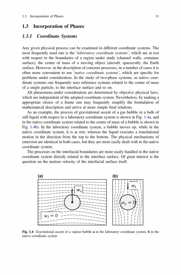
As an example, the process of gravitational ascent of a gas bubble in a bulk ofstill liquid with respect to a laboratory coordinate system is shown in Fig. 1.4a, andin the native coordinate system related to the centre of mass of a bubble is shown inFig. 1.4b). In the laboratory coordinate system, a bubble moves up, while in thenative coordinate system, it is at rest, whereas the liquid executes a translationalmotion in the direction from the top to the bottom. The physical mechanisms ofemersion are identical in both cases, but they are more easily dealt with in the nativecoordinate system.

The processes on the interfacial boundaries are more easily handled in the nativecoordinate system directly related to the interface surface. Of great interest is thequestion on the motion velocity of the interfacial surface itself.

(a) (b)

Fig. 1.4 Gravitational ascent of a vapour bubble a in the laboratory coordinate system, b in thenative coordinate system

1.3 Incorporation of Phases 11